Motion Control of a Robot Manipulator in Free Space … work/duchaine... · Space Based on Model...

7

Motion Control of a Robot Manipulator in Free Space Based on Model Predictive Control

Vincent Duchaine, Samuel Bouchard and Clément Gosselin Université Laval

Canada

1. Introduction The majority of existing industrial manipulators are controlled using PD controllers. This type of basically linear control does not represent an optimal solution for the motion control of robots in free space because robots exhibit highly nonlinear kinematics and dynamics. In fact, in order to accommodate configurations in which gravity and inertia terms reach their minimum amplitude, the gain associated with the derivative feedback (D) must be set to a relatively large value, thereby leading to a generally over-damped behaviour that limits the performance. Nevertheless, in most current robotic applications, PD controllers are functional and sufficient due to the high reduction ratio of the transmissions used. However, this assumption is no longer valid for manipulators with low transmission ratios such as human-friendly manipulators or those intended to perform high accelerations like parallel robots. Over the last few decades, a new control approach based on the so-called Model Predictive Control (MPC) algorithm was proposed. Arising from the work of Kalman (Kalman, 1960) in the 1960’s, predictive control can be said to provide the possibility of controlling a system using a proactive rather than reactive scheme. Since this control method is mainly based on the recursive computing of the dynamic model of the process over a certain time horizon, it naturally made its first successful breakthrough in slow linear processes. Common current applications of this approach are typically found in the petroleum and chemical industries. Several attempts were made to adapt this computationally intensive method to the control of robot manipulators. A little more than a decade ago, it was proposed to apply predictive control to nonlinear robotic systems (Berlin & Frank, 1991), (Compas et al., 1994). However, in the latter references, only a restricted form of predictive control was presented and the implementation issues — including the computational burden — were not addressed. Later, predictive control was applied to a broader variety of robotic systems such as a 2-DOF (degree-of-freedom) serial manipulator (Zhang & Wang, 2005), robots with flexible joints (Von Wissel et al., 1994), or electrical motor drives (Kennel et al., 1987). More recently, (Hedjar et al., 2005), (Hedjar & Boucher, 2005) presented simplified approaches using a limited Taylor expansion. Due to their relatively low computation time, the latter approaches open the avenue to real-time implementations. Finally, (Poignet & Gautier, 2000), (Vivas et al., 2003), (Lydoire & Poignet, 2005), experimentally demonstrated

Robot Manipulators

138

predictive control on a 4-DOF parallel mechanism using a linear model in the optimization combined with a feedback linearization. Several other control schemes based on the prediction of the torque to be applied at the actuators of a robot manipulator can be found in the literature. Probably the best-known and most commonly used technique is the so-called Computed Torque Method (Anderson, 1989), (Ubel et al., 1992). However, this control scheme has the disadvantage of not being robust to modelling errors. In addition to having the capability of making predictions over a certain time horizon, model predictive control contains a feedback mechanism compensating for prediction errors due to structural mismatch between the model and the process. These two characteristics make predictive control very efficient in terms of optimal control as well as very robust. This chapter aims at providing an introduction to the application of model predictive control to robot manipulators despite their typical nonlinear dynamics and fast servo rate. First, an overview of the theory behind model predictive control is provided. Then, the application of this method to robot control is investigated. After making some assumptions on the robot dynamics, equations for the cost function to be minimized are derived. The solution of these equations leads to an analytic and computationally efficient expression for position and velocity control which are functions of a given prediction time horizon and of the dynamic model of the robot. Finally, several experiments using a 1-DOF pendulum and a 6-DOF cable-driven parallel mechanism are presented in order to illustrate the performance in terms of dynamics as well as the computational efficiency.

2. Overview The very first predictive control schemes appeared around 1980 under the form of Dynamic Matrix Control (DMC) and Generalized Predictive Control (GPC). These two approaches led to a successful breakthrough in the chemical industry and opened the avenue to several new control algorithms later known as the family of model predictive control. A more detailed account of the history of model predictive control can be found in (Morari & Lee, 1999). Model predictive control is based on three main key ideas. These ideas have been well summarized by Camacho and Bordons in their book on the subject (Camacho & Bordons, 2004). This method is in fact based on the explicit use of a model to predict the process output at future time instants horizon. The prediction is done via the calculation of a control sequence minimizing an objective function. It also has the particularity that it is based on a receding strategy, so that at each instant the horizon is displaced toward the future, which involves the application of the first control signal of the sequence calculated at each step. This last particularity partially explains why predictive control is sometime called receding horizon control. As mentioned above, a predictive control scheme required the minimization of a quadratic cost function over a prediction horizon in order to predict the correct control input to be applied to the system. The cost function is composed of two parts, namely, a quadratic function of the deterministic and stochastic components of the process and a quadratic function of the constraints. The latter is one of the main advantages of this control method over many other schemes. It can deal at same time with model regulation and constraints. The constraints can be on the process as well as on the control output. The global function to be minimized can then be written in a general form as:


139

(1)

where

Although this function is the key of the effectiveness of the predictive control scheme in terms of optimal control, it is also its weakness in term of computational time. For linear processes, and depending on the constraint function, the optimal control sequence can be found relatively fast. However, for nonlinear model the problem is no longer convex and hence the computation of the function over the prediction horizon becomes computationally intensive and sometime very hard to solve explicitly.

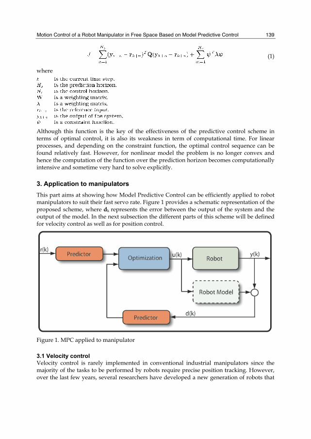
3. Application to manipulators This part aims at showing how Model Predictive Control can be efficiently applied to robot manipulators to suit their fast servo rate. Figure 1 provides a schematic representation of the proposed scheme, where dk represents the error between the output of the system and the output of the model. In the next subsection the different parts of this scheme will be defined for velocity control as well as for position control.

Figure 1. MPC applied to manipulator

3.1 Velocity control Velocity control is rarely implemented in conventional industrial manipulators since the majority of the tasks to be performed by robots require precise position tracking. However, over the last few years, several researchers have developed a new generation of robots that

Robot Manipulators

140

are capable of working in collaboration with humans (Berbardt et al., 2004), (Peshkin & Colgate, 2001), (Al-Jarrah & Zheng, 1996). For this type of tasks, velocity control seems more appropriate (Duchaine & Gosselin, 2007) due to the fact that the robot is not constrained to given positions but rather has to follow the movement of the human collaborator. Also, velocity control has infinitely spatial equilibrium points which is a very safe intrinsic behaviour in a context where a human being is sharing the workspace of a robot. The predictive control approach presented in this chapter can be useful in this context.

3.1.1 Modelling For velocity control, the reference input is usually relatively constant, especially considering the high servo rates used. Therefore, it is reasonable to assume that the reference velocity remains constant over the prediction horizon. With this assumption, the stochastic predictor of the reference velocity becomes:

(2)

where stands for the predicted value of r at time step j. The error, d, is obtained by computing the difference between the system's output and the model's output. Taking into account this difference in the cost function will help to increase the robustness of the control to model mismatch. The error can be decomposed in two parts. The first one is the error associated directly with model uncertainties. Often, this component will produce an offset proportional to the mismatch. The error may also include a zero-mean white noise given by the noise of the encoder or some random perturbation that cannot be included in the deterministic model. Since the error term is partially composed of zero-mean white noise, it is difficult to define a good stochastic predictor of the future values. However, in the case considered here, a future error equal to the present one will be simply assumed. This can be expressed as:

(3)

where is the predicted value of d at time step j. In this chapter, a constraint on the variation of the control input signal (u) over a prediction horizon will be used as a constraint function in the optimization. This is a typical constraint over the control input that helps smoothing the command and tends to maximize the effective life of the actuator, namely:

(4)

The model of the robot itself is directly linked with its dynamic behaviour. The dynamic equations of a robot manipulator can be expressed as:


141

(5)

Where

The acceleration resulting from a torque applied on the system can be found by inverting eq. (5), which leads to:

(6)

where and are the positions and velocities measured by the encoders. Assuming that the acceleration is constant over one time period, the above expression can be substituted into the equations associated with the motion of a body undergoing constant acceleration, which leads to:

(7)

where Ts is the sampling period. Since robots usually run on a discrete controller with a very small sampling period, assuming a constant acceleration over a sample period is a reasonable approximation that will not induce significant errors. Eq. (7) represents the behaviour of the robot over a sampling period. However, in predictive control, this behaviour must be determined over a number of sampling periods given by the horizon of prediction. Since the dynamic model of the manipulator is nonlinear, it is not straightforward to compute the necessary recurrence over this horizon, especially considering the limited computational time available. This is one of the reasons why predictive control is still not commonly used for manipulator control. Instead of computing exactly the nonlinear evolution of the manipulator dynamics, it can be more efficient to make some assumptions that will simplify the calculations. For the accelerations normally encountered in most manipulator applications, the gravitational term is the one that has the most impact on the dynamic model. The evolution of this term over time is a function of the position. The position is obtained by integrating the velocity over time. Even a large variation of velocity will not lead to a significant change of position since it is integrated over a very short period of time. From this point of view, the high sampling rate that is typically used in robot controllers allows us to assume that the nonlinear terms of the dynamic model are constant over a prediction horizon. Obviously, this assumption will induce some error, but this error can easily be managed by the error term included in the minimization. It is known from the literature that for an infinite prediction horizon and for a stabilizable process, as long as the objective function weighting matrices are positive definite, predictive control will always stabilize the system (Qin & Badgwell, 1997). However, the simplifications that have been made above on the representation of the system prevent us from concluding on stability since the errors in the model will increase nonlinearly with an increasing prediction horizon. It is not trivial to determine the duration of the prediction horizon that will ensure the stability of the control method. The latter will depend on the

Robot Manipulators

142

dynamic model, the geometric parameters and also on the conditioning of the manipulator at a given pose.

3.1.2 The optimization cost function From the above derivations, combining the deterministic and stochastic components and the constraint on the input variable leads to the general cost function to be optimized as a function of the prediction and control horizons. This function can be divided into two sums in order to manage distinctively the prediction horizon and control horizon. One has:

(8)

with

(9)

(10) being the integration form for of the linear equation (7) and where

An explicit solution to the minimization of J can be found for given values of Hp and Hc. However, it is more difficult to find a general solution that would be a function of Hp and Hc. Nevertheless, a minimum of J can easily be found numerically. From eq. (8), it is clear that J is a quadratic function of Γ. Moreover, because of its physical meaning, the minimum of J is reached when the derivative of J with respect to Γ is equal to zero. The problem can thus be reduced to finding the root of the following equation:

(11)

with

(12)

(13)

(14)

An exact and unique solution to this equation exists since it is linear. However, the computation of the solution involves the resolution of a system of linear equation whose size increases linearly with the control horizon. Another drawback of this approach is that


143

the generalized inertia matrix must be inverted, which can be time consuming. The next section will present strategies to avoid these drawbacks.

3.1.3 Analytical Solution of the minimization problem The previous section provided a general formulation of the MPC applied to robot manipulators with an arbitrary number of degrees of freedom and arbitrary chosen prediction and control horizons. However, in this section, only the prediction horizon will be considered, discarding the constraint function. This simplification of the general approach of the predictive control will make it possible to find an exact expression of the optimal control input signal for any prediction horizon thereby reducing drastically the computing time. Many predictive schemes presented in the literature (Berlin & Frank, 1991), (Hedjar et al., 2005), (Hedjar & Boucher, 2005) consider only the prediction horizon and disregard the control horizon, which simplifies greatly the formulation. Also, the constraint imposed on the input variable can be eliminated. At high servo rates, neglecting this constraint does not have a major impact since the input signal does not usually vary much from one period to another. Thus, the aggressiveness of the control variable Γ that will result from the elimination of the constraint function can easily be compensated for by the use of a longer prediction horizon. The above simplifications lead to a new cost function given by:

(15)

where

(16) Computing the derivative of eq. (15) with respect to Γ and setting it to zero, a general expression of the optimal control input signal as a function of the prediction horizon is obtained, namely:

(17)

The algebraic manipulations that lead to eq. (17) from eq. (15) are summarized in (Duchaine et al., 2007). Although this simplification leads to the loose of one of the main advantages of the MPC, the resulting control schemes will still exhibit good characteristics such as an easy tuning procedure, an optimal response and a better robustness to model mismatch compared to conventional computed torque control. It is noted also that this solution does not require the computation of the inverse of the generalized inertia matrix, thereby improving the computational efficiency. Moreover, since the solution is analytical, an online numerical optimization is no longer required.

3.2 Position control The position-tracking scheme of control follows a formulation similar to the one that was presented above for velocity control. The main differences are the stochastic predictor of the future reference position and the deterministic model of the manipulator that must now predict the future positions instead of velocities.

Robot Manipulators

144

3.2.1 Modelling In the velocity control scheme, it was assumed that the reference input was constant over the prediction horizon. This assumption was justified by the high servo rate and by the fact that the velocity does not usually vary drastically over a sampling period even in fast trajectories. However, this assumption cannot be used for position tracking. In particular, in the context of human-robot cooperation, no trajectory is established a priori and the future reference input must be predicted from current positions and velocities. A simple approximation that can be made is to use the time derivative of the reference to linearly predict its future. This can be written as:

(18)

where Δr is given by:

(19)

Since the error term d(k) is again partially composed of zero-mean white noise, one will consider the future of this error equal to the present. Therefore, eq. (4) is also used here. As shown in the previous section, the joint space velocity can be predicted using eq. (7). Integrating the latter equation once more with respect to time --- and assuming constant acceleration ---, the prediction on the position is obtained as:

(20)

3.2.2 The optimization cost function Including the deterministic model and the stochastic part inside the function to be minimized, the general function of predictive control for the manipulator is obtained:

(21)

with

(22)

Taking the derivative of this function with respect to Γ and setting it to zero leads to a linear equation where the root is the minimum of the cost function:

(23)


145

3.2.3 Exact Solution to the minimization Since the above result requires the use of a numerical procedure and also the inversion of the inertia matrix, the same assumptions that were made for simplifying the cost function for velocity control will be used again here. These assumptions lead to a simplified predictive control law that allows to find a direct solution to the minimization without using a numerical procedure. This function can be written as:

(24)

where

(25) Setting the derivative of this function with respect to u equal to zero and after some manipulations summarized in (Duchaine et al., 2007), the following optimal solution is obtained:

(26)

with

(27)

where Hp is the horizon of prediction. It is again pointed out that the direct solution of the minimization given by eq. (26) does not require the computation of the inverse of the inertia matrix.

4. Experimental demonstration The predictive control algorithm presented in this chapter aims at providing a more accurate control of robots. The first goal of the experiment is thus to compare the performance of the predictive controller to the performance of a PID controller on an actual robot. The second objective is to verify that the simplifying assumptions that were made in this paper hold in practice. The argument in favour of the predictive controller is that it should lead to better performances than a PID control scheme since it takes into account the dynamics of the robot and its futur behaviour while requiring almost the same computation time. In order to illustrate this phenomenon, the control algorithms were first used to actuate a simple 1-dof pendulum. Then, the position and velocity control were implemented on a 6-DOF cable-driven parallel mechanism. The controllers were implemented on a real time QNX computer with a servo rate of 500 Hz --- a typical servo rate for robotics applications. The PID controllers were tuned experimentally by minimizing the square norm of the error of the motors summed over the entire trajectories.

Robot Manipulators

146

4.1 Illustration with the 1-DOF pendulum A simple pendulum attached to a direct drive motor was controlled using a PID scheme and the predictive controller. This system, which represents one of the worst candidates for PID controllers, has been used to demonstrate how our assumption on the dynamical model does not affect the capability of the proposed predictive controller to stabilize nonlinear systems. The use of a direct drive motor maximizes the impact of the nonlinear terms of the dynamic model, making the system difficult to control by a conventional regulator. Also, the simplicity of the system helps to obtain accurate estimations of the parameters of the dynamic model that allow testing the ideal case. Despite the fact that its inertia remains constant over time, under constant angular velocity, the gravitational torque is the dominating term in the dynamic model. This setup also makes it possible to test the velocity control at high speed without having to consider angular limitations. Figure 2 provides the response of the system (angular velocity) to a given sequence of input reference velocities for the different controllers. The predictive control was implemented according to eq. (17) and an experimentally determined prediction horizon of four was used for the tests. It can be easily seen that PID control is inappropriate for this nonlinear dynamic mechanism. The sinusoidal error corresponds to the gravitational torque that varies with the rotation of the pendulum. The predictive control follows the reference input more adequately as it anticipates the variation of this term.

Figure 2. Speed response of the direct drive pendulum for PID and MPC control. (© 2007 IEEE)

4.2: 6-DOF cable-driven robot parallel A 6-DOF cable-driven robot with an architecture similar to the one presented in (Bouchard & Gosselin, 2007) is used in the experiment. It is shown in Fig.3 where the frame is a cube with two-meters edges. The end-effector is suspended by six cables. The cables are wound on pulleys actuated by motors fixed at the top of the frame.


147

Figure 3. Cable robot used in the experiment. (© 2007 IEEE)

4.2.1 Kinematic modeling For a given end-effector pose x the necessary cable lengths ρ can be calculated using the inverse kinematics. The length of cable i can be calculated by:

(28)

where

(29)

In eq. (29), bi and ai are respectively the position of the attachment point of cable i on the frame and on the end-effector, expressed in the global coordinate frame. Thus, vector ai can be expressed as:

(30)

a’i being the attachment point of cable i on the end-effector, expressed in the reference frame of the end-effector and Q being the rotation matrix expressing the orientation of the end-effector in the fixed reference frame. Vector c is defined as the position of the reference point on the end-effector in the fixed frame. Considering a fixed pulley radius r the cable length can be related to the angular positions θ of the actuators

(31)

Substituting ρ in eq. (28) and differentiating with respect to time, one obtains the velocity equation:

(32)

Robot Manipulators

148

where is the twist of the end-effector,

(33)

(34)

(35)

(36)

vector ci being

(37) and where ω is the angular velocity of the end-effector.

4.2.2 Dynamic modeling In this work, the cables are considered straight, massless and infinitely stiff. The assumption of straight cables is justified since the robot is small and the mass of the end-effector is much larger than the mass of the cables, which induces no sag. The measurements are made for chosen trajectories for which the cables are kept in tension at all times. The inertia of the wires is negligible compared to the combined inertia of the pulleys and end-effector. Although it is of research interest, the elasticity of the cables is not considered in the dynamic model for this work. The elastic behaviour is not exhibited strongly because of the high stiffness of the cables under relatively low accelerations (maximum 9.81 m/s2) of a 600g end-effector. Eq. (32) can be rearranged as

(38)

where

(39)

From eq. (38) and using the principle of virtual work, the following dynamic equation can be obtained:

(40)

where Ip is the inertia matrix of the pulleys and motors combined

(41)

Kν is the matrix of the viscous friction at the actuators

(42)


149

Me is the inertia matrix of the end-effector

(43) me being the mass of the end-effector and Ie its inertia matrix given by the CAD model. Vector wg is the wrench applied by gravity on the end-effector. By differentiating eq. (38) with respect to time, one obtains:

(44)

Substituting this expression for in eq. (40), the dynamics can be expressed with respect to the joint variables θ :

(45) Equation (45) has the same form as eq. (5) where

(46)

4.2.3 Trajectories The trajectories are defined in the Cartesian space. For the experiment, the selected trajectory is a displacement of 0.95 meter along the vertical axis performed in one second. The displacement follows a fifth order polynomial with respect to time, with zero speed and acceleration at the beginning and at the end. This smooth displacement is chosen in order to avoid inducing vibrations in the robot since the elasticity of the cables is not taken into account in the dynamic model. As mentioned earlier, it was verified prior to the experiment that this trajectory does not require compression in any of the cables. The cable robot is controlled using θ the joint coordinates and velocity of the pulleys. The Cartesian trajectories are thus converted in the joint space using the inverse kinematics and the velocity equations. A numerical solution to the direct kinematic problem is also implemented to determine the pose from the information of the encoders. This estimated pose is used to calculate the terms that depend on x.

4.3 Experimental results for the 6-DOF robot

4.3.1 Velocity control Figure 4 provides the error between the response of the system (joint velocities) and the time derivative of the joint trajectory described above for the two different controllers. The corresponding control input signals are also shown on this figure. The predictive control algorithm was implemented according to eq. (17) and an experimentally determined horizon of prediction Hp=11 was used. It can be observed that the magnitude of the error is smaller with the proposed predictive control than with the PID. The control input signals also appears to be smoother with the proposed approach than with the conventional linear controller. The PID suffers from the use of the second derivative of the encoder for the derivative gain (D) which reduces the

Robot Manipulators

150

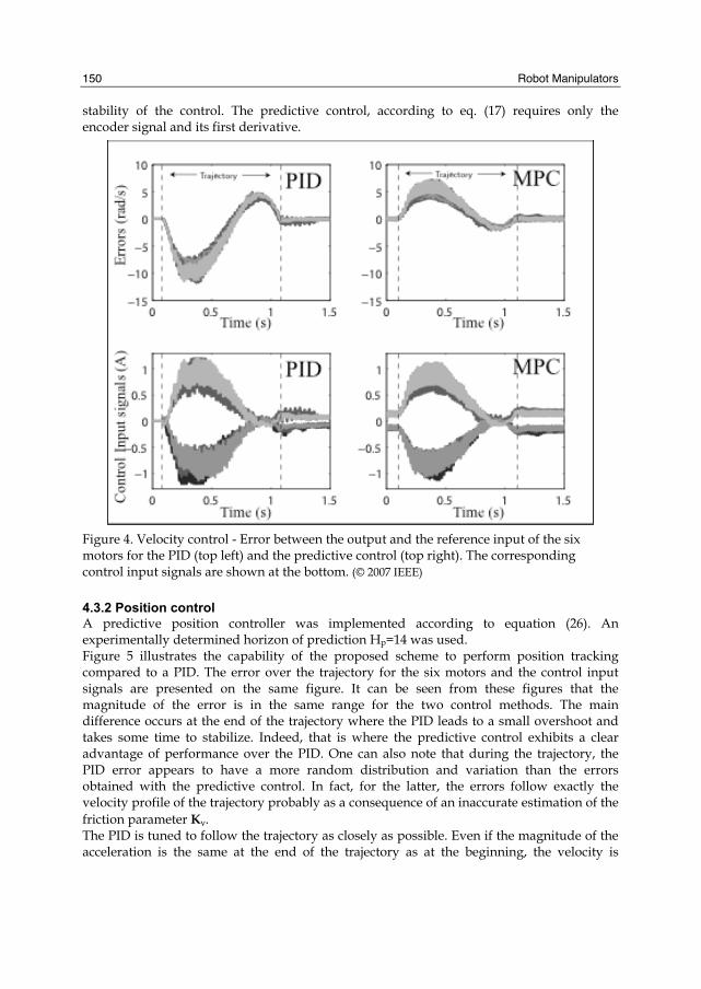
stability of the control. The predictive control, according to eq. (17) requires only the encoder signal and its first derivative.

Figure 4. Velocity control - Error between the output and the reference input of the six motors for the PID (top left) and the predictive control (top right). The corresponding control input signals are shown at the bottom. (© 2007 IEEE)

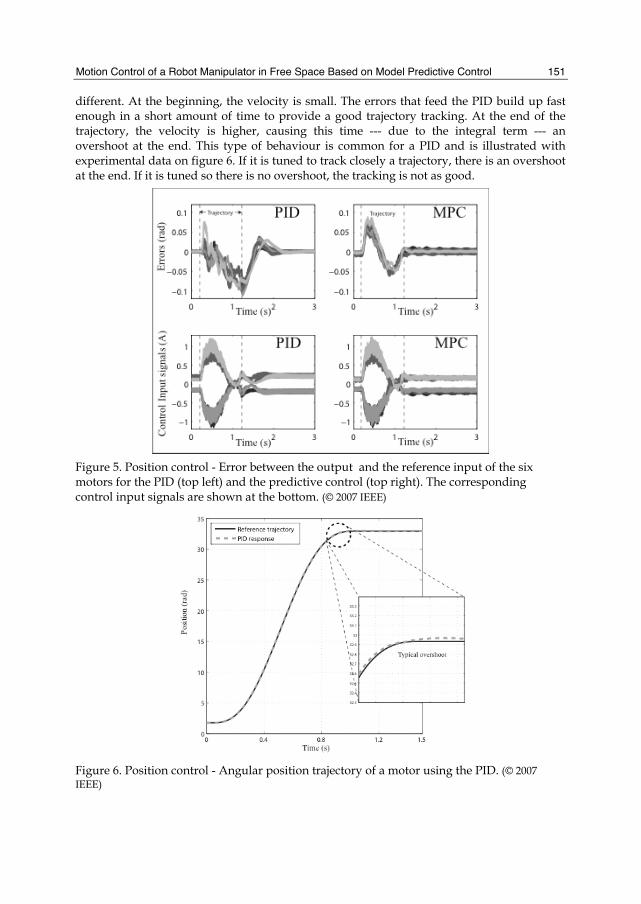
4.3.2 Position control A predictive position controller was implemented according to equation (26). An experimentally determined horizon of prediction Hp=14 was used. Figure 5 illustrates the capability of the proposed scheme to perform position tracking compared to a PID. The error over the trajectory for the six motors and the control input signals are presented on the same figure. It can be seen from these figures that the magnitude of the error is in the same range for the two control methods. The main difference occurs at the end of the trajectory where the PID leads to a small overshoot and takes some time to stabilize. Indeed, that is where the predictive control exhibits a clear advantage of performance over the PID. One can also note that during the trajectory, the PID error appears to have a more random distribution and variation than the errors obtained with the predictive control. In fact, for the latter, the errors follow exactly the velocity profile of the trajectory probably as a consequence of an inaccurate estimation of the friction parameter Kν. The PID is tuned to follow the trajectory as closely as possible. Even if the magnitude of the acceleration is the same at the end of the trajectory as at the beginning, the velocity is


151

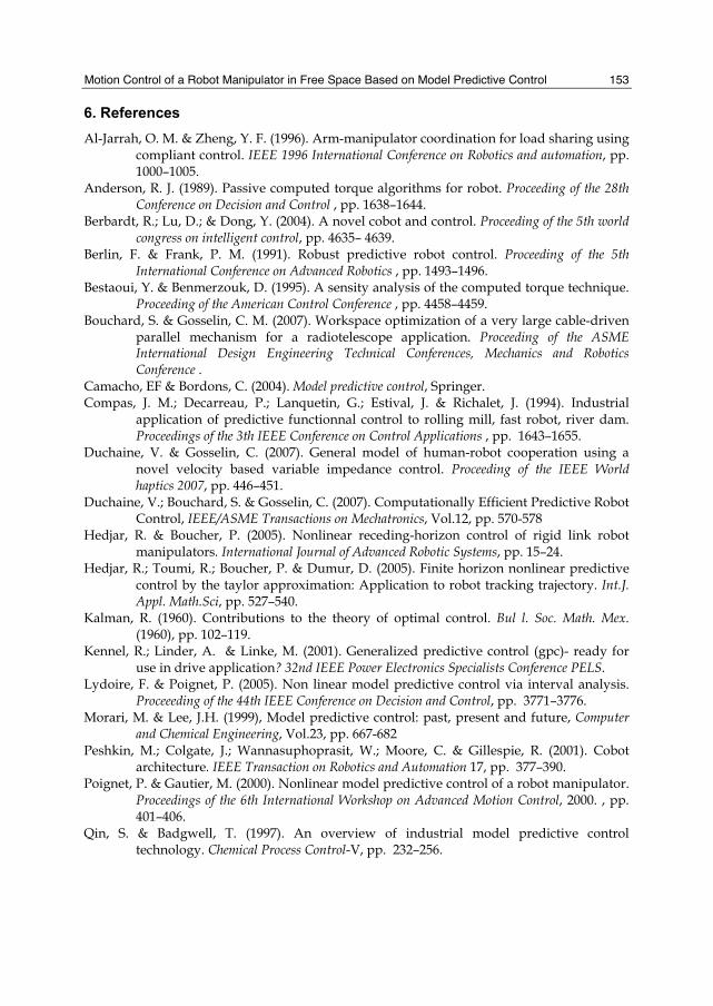
different. At the beginning, the velocity is small. The errors that feed the PID build up fast enough in a short amount of time to provide a good trajectory tracking. At the end of the trajectory, the velocity is higher, causing this time --- due to the integral term --- an overshoot at the end. This type of behaviour is common for a PID and is illustrated with experimental data on figure 6. If it is tuned to track closely a trajectory, there is an overshoot at the end. If it is tuned so there is no overshoot, the tracking is not as good.

Figure 5. Position control - Error between the output and the reference input of the six motors for the PID (top left) and the predictive control (top right). The corresponding control input signals are shown at the bottom. (© 2007 IEEE)

Figure 6. Position control - Angular position trajectory of a motor using the PID. (© 2007 IEEE)

Robot Manipulators

152

The predictive controller does not suffer from this problem. It is possible to have a controller that tracks closely a fast trajectory, without overshooting at the end. The reason is that the controller anticipates the required torques, the future reference input and takes into account the dynamics and the actual conditions of the system. Experimentally, another advantage of the predictive controller is that it appears to be much easier to tune than the PID. With a good dynamic model, only the prediction horizon has to be adjusted in order to obtain a controller that is more or less aggressive.

4.3.3 Computation time The computation time was also determined for each controller during position tracking. The results are given in table 1. The PID controller requires a longer calculation time at each step. The integrator in the RT-Lab/QNX computer consumes the most calculation time in the PID. Actually, if it is removed to obtain a PD controller, the computation time drops to 209 μs. Each controller requires computation times of the same order of magnitude. This means that it is fair to compare them with the same servo rate.

Controller Mean Computation time (μs)

PID controller 506

Predictive control 281

Table 1. Computation time required for each controller

5. Conclusion This chapter presented a simplified approach to predictive control adapted to robot manipulators. Control schemes were derived for velocity control as well as position tracking, leading to general predictive equations that do not require online optimization. Several justified simplifications were made on the deterministic part of the typical predictive control in order to obtain a compromise between the accuracy of the model and the computation time. These simplifications can be seen as a means of combining the advantages of predictive control with the simplicity of implementation of a computed torque method and the fast computing time of a PID. Despite all these simplifications, experimental results on a 6-DOF cable-driven parallel manipulator demonstrated the effectiveness of the method in terms of performance. The method using the exact solution of the optimal control appears to alleviate two of the main drawbacks of predictive control for manipulators, namely: the complexity of the implementation and the computational burden.Further investigations should focus on the stability analysis using Lyapunov functions and also on the demonstration of the robustness of the proposed control law.


153

6. References Al-Jarrah, O. M. & Zheng, Y. F. (1996). Arm-manipulator coordination for load sharing using

compliant control. IEEE 1996 International Conference on Robotics and automation, pp. 1000–1005.

Anderson, R. J. (1989). Passive computed torque algorithms for robot. Proceeding of the 28th Conference on Decision and Control , pp. 1638–1644.

Berbardt, R.; Lu, D.; & Dong, Y. (2004). A novel cobot and control. Proceeding of the 5th world congress on intelligent control, pp. 4635– 4639.

Berlin, F. & Frank, P. M. (1991). Robust predictive robot control. Proceeding of the 5th International Conference on Advanced Robotics , pp. 1493–1496.

Bestaoui, Y. & Benmerzouk, D. (1995). A sensity analysis of the computed torque technique. Proceeding of the American Control Conference , pp. 4458–4459.

Bouchard, S. & Gosselin, C. M. (2007). Workspace optimization of a very large cable-driven parallel mechanism for a radiotelescope application. Proceeding of the ASME International Design Engineering Technical Conferences, Mechanics and Robotics Conference .

Camacho, EF & Bordons, C. (2004). Model predictive control, Springer. Compas, J. M.; Decarreau, P.; Lanquetin, G.; Estival, J. & Richalet, J. (1994). Industrial

application of predictive functionnal control to rolling mill, fast robot, river dam. Proceedings of the 3th IEEE Conference on Control Applications , pp. 1643–1655.

Duchaine, V. & Gosselin, C. (2007). General model of human-robot cooperation using a novel velocity based variable impedance control. Proceeding of the IEEE World haptics 2007, pp. 446–451.

Duchaine, V.; Bouchard, S. & Gosselin, C. (2007). Computationally Efficient Predictive Robot Control, IEEE/ASME Transactions on Mechatronics, Vol.12, pp. 570-578

Hedjar, R. & Boucher, P. (2005). Nonlinear receding-horizon control of rigid link robot manipulators. International Journal of Advanced Robotic Systems, pp. 15–24.

Hedjar, R.; Toumi, R.; Boucher, P. & Dumur, D. (2005). Finite horizon nonlinear predictive control by the taylor approximation: Application to robot tracking trajectory. Int.J. Appl. Math.Sci, pp. 527–540.

Kalman, R. (1960). Contributions to the theory of optimal control. Bul l. Soc. Math. Mex. (1960), pp. 102–119.

Kennel, R.; Linder, A. & Linke, M. (2001). Generalized predictive control (gpc)- ready for use in drive application? 32nd IEEE Power Electronics Specialists Conference PELS.

Lydoire, F. & Poignet, P. (2005). Non linear model predictive control via interval analysis. Proceeeding of the 44th IEEE Conference on Decision and Control, pp. 3771–3776.

Morari, M. & Lee, J.H. (1999), Model predictive control: past, present and future, Computer and Chemical Engineering, Vol.23, pp. 667-682

Peshkin, M.; Colgate, J.; Wannasuphoprasit, W.; Moore, C. & Gillespie, R. (2001). Cobot architecture. IEEE Transaction on Robotics and Automation 17, pp. 377–390.

Poignet, P. & Gautier, M. (2000). Nonlinear model predictive control of a robot manipulator. Proceedings of the 6th International Workshop on Advanced Motion Control, 2000. , pp. 401–406.

Qin, S. & Badgwell, T. (1997). An overview of industrial model predictive control technology. Chemical Process Control-V, pp. 232–256.

Robot Manipulators

154

Uebel, M., Minis, I., and Cleary, K. (1992). Improved computed torque control for industrial robots. International Conference on Robotics and Automation, pp. 528–533.

Vivas, A., Poignet, P., and Pierrot, F. (2003). Predictive functional control for a parallel robot. Proceedings of the International Conference on Intelligent Robots and Systems, pp. 2785–2790.

Von Wissel, D., Nikoukhah, R., and Campbell, S. L. (1994). On a new predictive control strategy: Application to a flexible-joint robot. Proceedings of the IEEE Conference on Decision and Control, pp. 3025–3026.

Zhang, Z., and Wang, W. (2005). Predictive function control of a two links robot manipulator. Proceeding of the Int. Conf. on Mechatronics and Automation, pp. 2004 – 2009.

Motion Control of a Robot Manipulator in Free Space … work/duchaine... · Space Based on Model...

Documents

Transcript of Motion Control of a Robot Manipulator in Free Space … work/duchaine... · Space Based on Model...