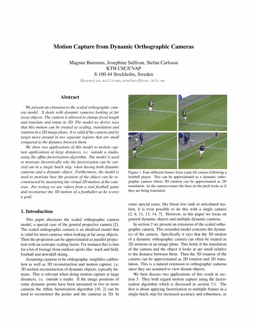
Motion Capture from Dynamic Orthographic Cameras

Magnus Burenius, Josephine Sullivan, Stefan CarlssonKTH CSC/CVAP

S-100 44 Stockholm, Sweden{burenius,sullivan,stefanc}@csc.kth.se

Abstract

We present an extension to the scaled orthographic cam-era model. It deals with dynamic cameras looking at faraway objects. The camera is allowed to change focal lengthand translate and rotate in 3D. The model we derive saysthat this motion can be treated as scaling, translation androtation in a 2D image plane. It is valid if the camera and itstarget move around in two separate regions that are smallcompared to the distance between them.

We show two applications of this model to motion cap-ture applications at large distances, i.e. outside a studio,using the affine factorization algorithm. The model is usedto motivate theoretically why the factorization can be car-ried out in a single batch step, when having both dynamiccameras and a dynamic object. Furthermore, the model isused to motivate how the position of the object can be re-constructed by measuring the virtual 2D motion of the cam-eras. For testing we use videos from a real football gameand reconstruct the 3D motion of a footballer as he scoresa goal.

1. IntroductionThis paper discusses the scaled orthographic camera

model, a special case of the general projective camera [2].The scaled orthographic camera is an idealized model thatis valid for most cameras when looking at far away objects.Then the projection can be approximated as parallel projec-tion with an isotropic scaling factor. For instance this is truefor a lot of footage from outdoor sports like: track and field,football and downhill skiing.

Assuming cameras to be orthographic simplifies calibra-tion as well as 3D reconstruction and motion capture, i.e.3D motion reconstruction of dynamic objects, typically hu-mans. This is relevant when doing motion capture at largedistances, i.e. outside a studio. If the image positions ofsome dynamic points have been measured in two or morecameras the Affine factorization algorithm [10, 2] can beused to reconstruct the points and the cameras in 3D. In

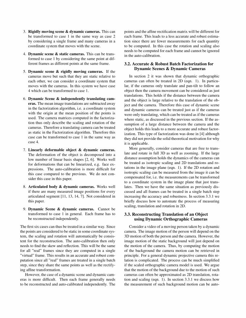
Figure 1. Four different frames from a pan tilt camera following afootball player. This can be approximated as a dynamic ortho-graphic camera whose 3D rotation can be approximated as 2Dtranslation. As the camera rotates the lines on the pitch looks as ifthey are being translated.

some special cases, like linear low rank or articulated mo-tion, it is even possible to do this with a single camera[2, 6, 11, 13, 14, 7]. However, in this paper we focus ongeneral dynamic objects and multiple dynamic cameras.

In section 2 we present an extension of the scaled ortho-graphic camera. This extended model concerns the dynam-ics of the camera. Specifically it says that the 3D motionof a dynamic orthographic camera can often be treated as2D motions in an image plane. This holds if the translationof the camera and the object it looks at are small relativeto the distance between them. Then the 3D rotation of thecamera can be approximated as 2D rotation and 2D trans-lation. This is a natural extension to orthographic camerassince they are assumed to view distant objects.

We then discuss two applications of this result in sec-tion 3. They both regard motion capture using the factor-ization algorithm which is discussed in section 3.1. Thefirst is about applying factorization to multiple frames in asingle batch step for increased accuracy and robustness, as

opposed to doing it independently for each frame. We mo-tivate theoretically why this can be done even if both theobject and cameras are dynamic in section 3.2.

The second application is about computing the positionof a reconstructed dynamic object (section 3.3). This de-pends on the absolute motion of the camera, which is diffi-cult to measure for a general projective camera. However,using the result that the motion of orthographic cameras canbe treated in 2D this process is simplified.

The related topic of detecting the isotropic scaling, 2Dtranslation and 2D rotations that relates a pair of images isbriefly discussed in section 3.3.1. Videos from a real foot-ball game are used for testing the motion capture in section4.

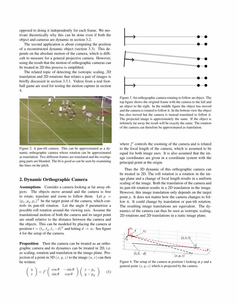
Figure 2. A pan-tilt camera. This can be approximated as a dy-namic orthographic camera whose rotation can be approximatedas translation. Two different frames are translated and the overlap-ping parts are blended. The fit is good as can be seen by examiningthe lines on the pitch.

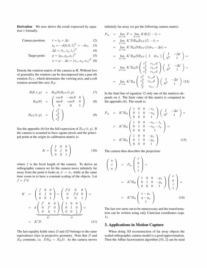
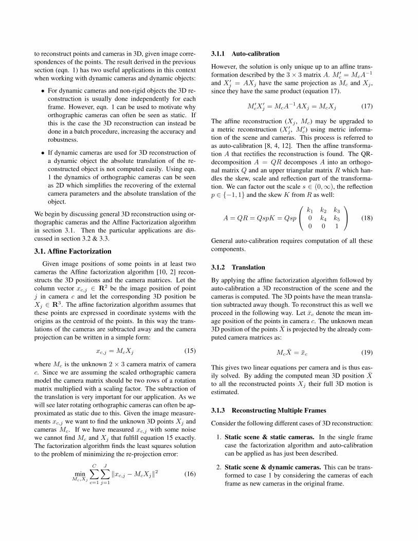
2. Dynamic Orthographic CameraAssumptions Consider a camera looking at far away ob-jects. The objects move around and the camera is freeto rotate, translate and zoom to follow them. Let p =(px, py, pz)T be the target point of the camera, which con-trols its pan-tilt rotation. Let the angle θ parametrize apossible roll rotation around the viewing axis. Assume thetranslational motion of both the camera and its target pointare small relative to the distance between the camera andthe objects. This can be modeled by placing the camera atposition t = (tx, ty, tz−d)T and letting d→∞. See figure4 for the setup of the camera.

Proposition Then the camera can be treated as an ortho-graphic camera and its dynamics can be treated in 2D, i.e.as scaling, rotation and translation in the image plane. Pro-jection of a point in 3D (x, y, z) to the image (u, v) can thenbe written:(

uv

)= f ′

(cos θ − sin θsin θ cos θ

)(x− pxy − py

)(1)

Figure 3. An orthographic camera rotating to follow an object. Thetop figure shows the original frame with the camera to the left andan object to the right. In the middle figure the object has movedand the camera is rotated to follow it. In the bottom view the objecthas also moved but the camera is instead translated to follow it.The projected image is approximately the same. If the object isinfinitely far away the result will be exactly the same. The rotationof the camera can therefore be approximated as translation.

where f ′ controls the zooming of the camera and is relatedto the focal length of the camera, which is assumed to beequal for both image axes. It is also assumed that the im-age coordinates are given in a coordinate system with theprincipal point at the origin.

Thus the 3D dynamic of this orthographic camera canbe treated in 2D. The roll rotation is a rotation in the im-age plane and a change of focal length results in a uniformscaling of the image. Both the translation of the camera andits pan-tilt rotation results in a 2D translation in the image.However, this image translation only depends on the targetpoint p. It does not matter how the camera changes to fol-low it. It could change by translation or pan-tilt rotation.The resulting image translations are equivalent. The dy-namics of the camera can thus be seen as isotropic scaling,2D rotations and 2D translations in a static image plane.

Figure 4. The setup of the camera at position t looking at p and ageneral point (x, y, z) which is projected by the camera.

Derivation We now derive the result expressed by equa-tion 1 formally:

Camera position: t = t0 + ∆t (2)t0 = −d(0, 0, 1)T = −de3 (3)∆t = (tx, ty, tz)T (4)

Target point: p = (px, py, pz)T (5)n = p−∆t = (nx, ny, nz)T (6)

Denote the rotation matrix of the camera as R. Without lossof generality the rotation can be decomposed into a pan-tiltrotationRPT , which determines the viewing axis, and a rollrotation around this axis RR:

R(θ, t, p) = RR(θ)RPT (t, p) (7)

RR(θ) =

cos θ − sin θ 0sin θ cos θ 0

0 0 1

(8)

RPT (t, p) =

rT1rT2rT3

(9)

See the appendix (6) for the full expression of RPT (t, p). Ifthe camera is assumed to have square pixels and the princi-pal point at the origin its calibration matrix is:

K =

f 0 00 f 00 0 1

(10)

where f is the focal length of the camera. To derive anorthographic camera we let the camera move infinitely faraway from the point it looks at, d → ∞, while at the sametime zoom in to have a constant scaling of the objects. Letf = f ′d:

K =

f 0 00 f 00 0 1

=

f ′d 0 00 f ′d 00 0 1

=

= d

f ′ 0 00 f ′ 00 0 1

︸ ︷︷ ︸

K′

1 0 00 1 00 0 1

d

︸ ︷︷ ︸

D

=

= K ′D (11)

The last equality holds since D and dD belongs to the sameequivalence class in projective geometry. Note that D andRR commute, i.e. DRR = RRD. As the camera moves

infinitely far away we get the following camera matrix:

P∞ = limd→∞

P = limd→∞

KR(I| − t) =

= limd→∞

K ′DRRRPT (I| − t) =

= limd→∞

K ′RRDRPT (I|de3 −∆t) =

= limd→∞

K ′RRDRPT

(I de3

)( I −∆t0T 1

)=

= limd→∞

K ′RRD

rT1 r1,zdrT2 r2,zdrT3 r3,zd

( I −∆t0T 1

)=

= limd→∞

K ′RR

rT1 r1,zdrT2 r2,zdrT3d r3,z

( I −∆t0T 1

)(12)

In the final line of equation 12 only one of the matrices de-pends on d. The limit value of this matrix is computed inthe appendix (6). The result is:

P∞ = K ′RR

1 0 0 −nx0 1 0 −ny0 0 0 1

( I −∆t0T 1

)=

= K ′RR

1 0 0 −nx − tx0 1 0 −ny − ty0 0 0 1

=

= K ′RR

1 0 0 −px0 1 0 −py0 0 0 1

(13)

The camera thus describes the projection:

uvw

= P∞

xyz1

=

= K ′RR

1 0 0 −px0 1 0 −py0 0 0 1

xyz1

=

= K ′RR

x− pxy − py

1

(14)

The last row turns out to be unnecessary and the transforma-tion can be written using only Cartesian coordinates (eqn.1).

3. Applications in Motion CaptureWhen doing 3D reconstruction of far away objects the

scaled orthographic camera model is a good approximation.Then the Affine factorization algorithm [10, 2] can be used

to reconstruct points and cameras in 3D, given image corre-spondences of the points. The result derived in the previoussection (eqn. 1) has two useful applications in this contextwhen working with dynamic cameras and dynamic objects:

• For dynamic cameras and non-rigid objects the 3D re-construction is usually done independently for eachframe. However, eqn. 1 can be used to motivate whyorthographic cameras can often be seen as static. Ifthis is the case the 3D reconstruction can instead bedone in a batch procedure, increasing the accuracy androbustness.

• If dynamic cameras are used for 3D reconstruction ofa dynamic object the absolute translation of the re-constructed object is not computed easily. Using eqn.1 the dynamics of orthographic cameras can be seenas 2D which simplifies the recovering of the externalcamera parameters and the absolute translation of theobject.

We begin by discussing general 3D reconstruction using or-thographic cameras and the Affine Factorization algorithmin section 3.1. Then the particular applications are dis-cussed in section 3.2 & 3.3.

3.1. Affine Factorization

Given image positions of some points in at least twocameras the Affine factorization algorithm [10, 2] recon-structs the 3D positions and the camera matrices. Let thecolumn vector xc,j ∈ R2 be the image position of pointj in camera c and let the corresponding 3D position beXj ∈ R3. The affine factorization algorithm assumes thatthese points are expressed in coordinate systems with theorigins as the centroid of the points. In this way the trans-lations of the cameras are subtracted away and the cameraprojection can be written in a simple form:

xc,j = McXj (15)

where Mc is the unknown 2 × 3 camera matrix of camerac. Since we are assuming the scaled orthographic cameramodel the camera matrix should be two rows of a rotationmatrix multiplied with a scaling factor. The subtraction ofthe translation is very important for our application. As wewill see later rotating orthographic cameras can often be ap-proximated as static due to this. Given the image measure-ments xc,j we want to find the unknown 3D points Xj andcameras Mc. If we have measured xc,j with some noisewe cannot find Mc and Xj that fulfill equation 15 exactly.The factorization algorithm finds the least squares solutionto the problem of minimizing the re-projection error:

minMc,Xj

C∑c=1

J∑j=1

‖xc,j −McXj‖2 (16)

3.1.1 Auto-calibration

However, the solution is only unique up to an affine trans-formation described by the 3× 3 matrix A. M ′c = McA

−1

and X ′j = AXj have the same projection as Mc and Xj ,since they have the same product (equation 17).

M ′cX′j = McA

−1AXj = McXj (17)

The affine reconstruction (Xj , Mc) may be upgraded toa metric reconstruction (X ′j , M ′c) using metric informa-tion of the scene and cameras. This process is referred toas auto-calibration [8, 4, 12]. Then the affine transforma-tion A that rectifies the reconstruction is found. The QR-decomposition A = QR decomposes A into an orthogo-nal matrix Q and an upper triangular matrix R which han-dles the skew, scale and reflection part of the transforma-tion. We can factor out the scale s ∈ (0,∞), the reflectionp ∈ {−1, 1} and the skew K from R as well:

A = QR = QspK = Qsp

k1 k2 k30 k4 k50 0 1

(18)

General auto-calibration requires computation of all thesecomponents.

3.1.2 Translation

By applying the affine factorization algorithm followed byauto-calibration a 3D reconstruction of the scene and thecameras is computed. The 3D points have the mean transla-tion subtracted away though. To reconstruct this as well weproceed in the following way. Let x̄c denote the mean im-age position of the points in camera c. The unknown mean3D position of the points X̄ is projected by the already com-puted camera matrices as:

McX̄ = x̄c (19)

This gives two linear equations per camera and is thus eas-ily solved. By adding the computed mean 3D position X̄to all the reconstructed points Xj their full 3D motion isestimated.

3.1.3 Reconstructing Multiple Frames

Consider the following different cases of 3D reconstruction:

1. Static scene & static cameras. In the single framecase the factorization algorithm and auto-calibrationcan be applied as has just been described.

2. Static scene & dynamic cameras. This can be trans-formed to case 1 by considering the cameras of eachframe as new cameras in the original frame.

3. Rigidly moving scene & dynamic cameras. This canbe transformed to case 1 in the same way as case 2by considering a single frame and many cameras in acoordinate system that moves with the scene.

4. Dynamic scene & static cameras. This can be trans-formed to case 1 by considering the same point at dif-ferent frames as different points at the same frame.

5. Dynamic scene & rigidly moving cameras. If thecameras move but such that they are static relative toeach other, we can consider a coordinate system thatmoves with the cameras. In this system we have case4 which can be transformed to case 1.

6. Dynamic Scene & independently translating cam-eras. The mean image translations are subtracted awayin the factorization algorithm, i.e. a coordinate systemwith the origin at the mean position of the points isused. The camera matrices computed in the factoriza-tion thus only describe the scaling and rotation of thecameras. Therefore a translating camera can be treatedas static in the Factorization algorithm. Therefore thiscase can be transformed to case 1 in the same way ascase 4.

7. Linearly deformable object & dynamic cameras.The deformation of the object is decomposed into alow number of linear basis shapes [2, 6]. Works wellfor deformations that can be linearized, e.g. face ex-pressions. The auto-calibration is more difficult forthis case compared to the previous. We do not con-sider this case in this paper.

8. Articulated body & dynamic cameras. Works wellif there are many measured image positions for everyarticulated segment [11, 13, 14, 7]. Not considered inthis paper.

9. Dynamic Scene & dynamic cameras. Cannot betransformed to case 1 in general. Each frame has tobe reconstructed independently.

The first six cases can thus be treated in a similar way. Sincethe points are considered to be static in some coordinate sys-tem, the scaling and rotation will automatically be consis-tent for the reconstruction. The auto-calibration then onlyneeds to find the skew and reflection. This will be the samefor all ”real” frames since they are computed in a single”virtual” frame. This results in an accurate and robust com-putation since all ”real” frames are treated in a single batchstep, since they share the same points as well as the rectify-ing affine transformation.

However, the case of a dynamic scene and dynamic cam-eras is more difficult. Then each frame generally needsto be reconstructed and auto-calibrated independently. The

points and the affine rectification matrix will be different foreach frame. This leads to a less accurate and robust estima-tion since there are fewer measurements for each quantityto be computed. In this case the rotation and scaling alsoneeds to be computed for each frame and cannot be ignoredin the auto-calibration.

3.2. Accurate & Robust Batch Factorization forDynamic Scenes & Dynamic Cameras

In section 2 it was shown that dynamic orthographiccameras can often be treated in 2D (eqn. 1). In particu-lar, if the cameras only translate and pan-tilt to follow anobject then the camera movement can be considered as justtranslations. This holds if the distance between the cameraand the object is large relative to the translation of the ob-ject and the camera. Therefore this case of dynamic sceneand dynamic cameras can be treated just as if the cameraswere only translating, which can be treated as if the cameraswhere static, as discussed in the previous section. If the as-sumption of a large distance between the camera and theobject holds this leads to a more accurate and robust factor-ization. This type of factorization was done in [4] althoughthey did not provide the solid theoretical motivation for whyit is applicable.

More generally, consider cameras that are free to trans-late and rotate in full 3D as well as zooming. If the largedistance assumption holds the dynamics of the cameras canbe treated as isotropic scaling and 2D translations and ro-tations in the image plane (eqn. 1). If the 2D rotation andisotropic scaling can be measured from the image it can becompensated for, i.e. the measurements can be transformedto a coordinate system in the image plane that just trans-lates. Then we have the same situation as previously dis-cussed and all frames can be treated in a single batch stepincreasing the accuracy and robustness. In section 3.3.1 webriefly discuss how to automate the process of measuringscaling, translation and rotation in 2D.

3.3. Reconstructing Translation of an Objectusing Dynamic Orthographic Cameras

Consider a video of a moving person taken by a dynamiccamera. The image motion of the person will depend on the3D motion of both the person and the camera. However, theimage motion of the static background will just depend onthe motion of the camera. Thus, by computing the motionof the background the camera motion can be retrieved inprinciple. For a general dynamic projective camera this re-lation is complicated. The process can be much simplifiedif the scaled orthographic camera model is used. We arguethat the motion of the background due to the motion of suchcameras can often be approximated as 2D translation, rota-tion and scaling (eqn. 1). In section 3.3.1 we discuss howthe measurement of such background motion can be auto-

mated. For now we assume this has been measured.As described in sections 3.1 & 3.2 the factorization algo-

rithm can be used to reconstruct the cameras and the object.This is done by first transforming the measurements to a co-ordinate system where the camera only translates. Then thistranslation is also subtracted away before performing thefactorization. If the cameras are static then the 3D trans-lation can be added to the reconstruction as described insection 3.1.2.

But if the cameras are dynamic this approach is not di-rectly applicable. But since the cameras can be treated asonly translating we can add the camera translation to themeasured image mean position to have them in an absolutecoordinate system. Let mc,t denote the image translation ofcamera c at time t, where the first frame is chosen as zero.Let x̂c,t denote the measured mean image position of thepoints in camera c at time t, relative the camera translationat the same frame. Let x̄c,t denote the mean image posi-tion of the points in a coordinate system that is fixed for allframes which can then be computed as: x̄c,t = x̂c,t +mc,t.Then it is possible to proceed as previously described in sec-tion 3.1.2 and the full translation can be computed for the3D reconstruction even though the cameras are dynamic.

3.3.1 Measuring Image Translation, Rotation & Scale

Consider a pair of images that are approximately related bya 2D similarity transformation, i.e. isotropic scaling andtranslation and rotation in 2D. In this section we briefly dis-cuss how to compute this transformation from the two im-ages. This is related to the well studied problem of takinga set of overlapping images and making a panorama. Thiscan be considered a solved problem if there is not a lot ofdynamic objects or motion blur in the images [1]. However,this will typically not be the case when background motionis to be detected in a motion capture application.

Typically when doing 3D reconstruction the first step isto extract a lot of localized features in the images, e.g. SIFT,and then use RANSAC to find corresponding features andthe transformation that relates the images [2, 1]. A difficultyof doing this in our application is to differentiate the featuresbelonging to the object from the features of the background.Another difficulty in e.g. a football application is that thebackground might not have distinct features (fig. 1 & 2).

Another algorithm that is more specialized for measuring2D similarity transformation is Phase correlation [3, 9, 5].It utilizes the properties of the Fourier-transform and takesall pixels into account instead of just looking at distinct lo-calized features. A Phase correlation based approach cantherefore work as long as the background has some textureeven though it lack distinct localized features. Nevertheless,dealing with dynamic objects and motion blur in a robustway is still a complicated and unsolved problem.

4. Experiment

To test the result of section 2 and its applications dis-cussed in section 3 a football game was recorded bythree video cameras filming at 25 Hz and a resolution of1920x1080 pixels. One of the cameras was placed on thestand behind the goal and the other cameras on the standson each long side. The cameras had static positions but con-stantly rotated to follow a player and occasionally changedtheir zooming.

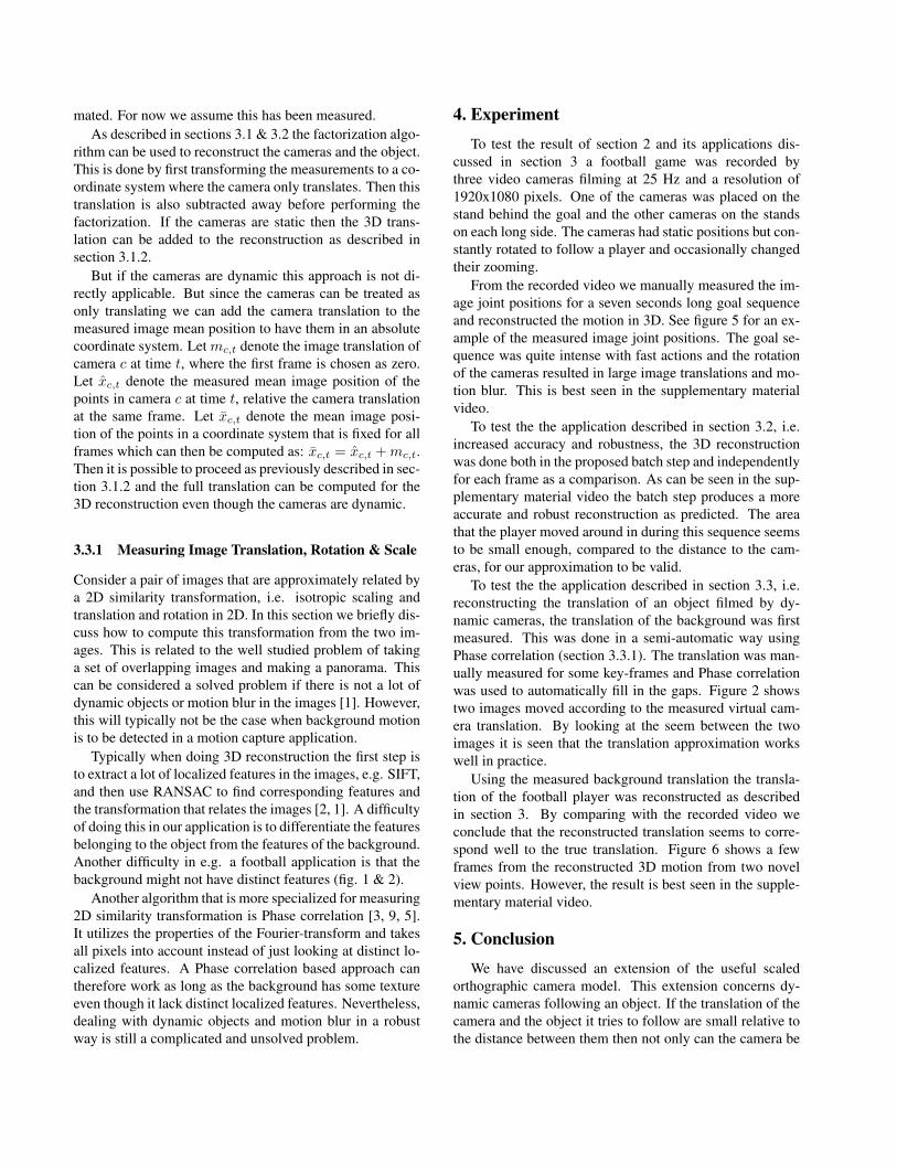
From the recorded video we manually measured the im-age joint positions for a seven seconds long goal sequenceand reconstructed the motion in 3D. See figure 5 for an ex-ample of the measured image joint positions. The goal se-quence was quite intense with fast actions and the rotationof the cameras resulted in large image translations and mo-tion blur. This is best seen in the supplementary materialvideo.

To test the the application described in section 3.2, i.e.increased accuracy and robustness, the 3D reconstructionwas done both in the proposed batch step and independentlyfor each frame as a comparison. As can be seen in the sup-plementary material video the batch step produces a moreaccurate and robust reconstruction as predicted. The areathat the player moved around in during this sequence seemsto be small enough, compared to the distance to the cam-eras, for our approximation to be valid.

To test the the application described in section 3.3, i.e.reconstructing the translation of an object filmed by dy-namic cameras, the translation of the background was firstmeasured. This was done in a semi-automatic way usingPhase correlation (section 3.3.1). The translation was man-ually measured for some key-frames and Phase correlationwas used to automatically fill in the gaps. Figure 2 showstwo images moved according to the measured virtual cam-era translation. By looking at the seem between the twoimages it is seen that the translation approximation workswell in practice.

Using the measured background translation the transla-tion of the football player was reconstructed as describedin section 3. By comparing with the recorded video weconclude that the reconstructed translation seems to corre-spond well to the true translation. Figure 6 shows a fewframes from the reconstructed 3D motion from two novelview points. However, the result is best seen in the supple-mentary material video.

5. Conclusion

We have discussed an extension of the useful scaledorthographic camera model. This extension concerns dy-namic cameras following an object. If the translation of thecamera and the object it tries to follow are small relative tothe distance between them then not only can the camera be

Figure 5. The manually measured image joint positions from a football goal sequence filmed by three rotating cameras.

Figure 6. 3D reconstruction of a football goal sequence shown from a novel view point. The result is best seen in color.

approximated as orthographic but its dynamic can be treatedin 2D.

This is relevant when doing motion capture at large dis-tances, i.e. outside a studio. In those scenarios the affinefactorization algorithm can be used to reconstruct the mo-tion in 3D. If dynamic cameras are used to capture the mo-tion of a dynamic object the factorization is generally doneindependently for each frame and also the absolute transla-tion of the object is lost.

Using the extended orthographic model we motivatedhow the factorization can be applied for all frames in a batchprocedure for increased accuracy and robustness. We alsoused it to motivate how the absolute translation of the objectcan be reconstructed by measuring the approximate 2D mo-tion of the background. Videos from a real football gamewere used for testing. In our experiments we used manualmeasurements. A natural and interesting future work is toautomate the measuring process.

6. AppendixNotation for cross product:

a× b = [a]×b (20)

[a]× =

0 −az ayaz 0 −ax−ay ax 0

(21)

The view direction is determined by r3:

r3 =p− t‖p− t‖

=p− t0 −∆t

‖p− t0 −∆t)‖=

=n− t0‖n− t0‖

=n+ de3‖n+ de3‖

=

=nd + e3

‖nd + e3‖=(nd

+ e3

)g(d) (22)

g(d) =1

‖nd + e3‖(23)

Since RPT should describe a pan-tilt rotation r1 should beorthogonal to both r3 and the unit vector along the y-axis:

r1 =e2 × r3‖e2 × r3‖

=1

‖e2 × r3‖

0 0 10 0 0−1 0 0

r3 =

=(r3,z, 0,−r3,x)T√

r23,z + r23,x

= (r3,z, 0,−r3,x)Th(d) (24)

h(d) =1√

r23,z + r23,x

(25)

The remaining row r2 should be orthogonal to r1 and r3:

r2 = −r1 × r3 =

= −h(d)

0 r3,x 0−r3,x 0 −r3,z

0 r3,z 0

r3 =

= (−r3,xr3,y, r23,z + r23,x,−r3,yr3,z)Th(d) (26)

As the camera moves infinitely far away we want to com-pute the following limit value:

limd→∞

rT1 r1,zdrT2 r2,zdrT3d r3,z

=

1 0 0 −nx0 1 0 −ny0 0 0 1

(27)

This was done as follows:

limd→∞

g(d) = limd→∞

1

‖nd + e3‖= 1 (28)

limd→∞

rT3 = limd→∞

(nd

+ e3

)g(d) = e3 = (0, 0, 1) (29)

limd→∞

rT3d

= limd→∞

e3d

= (0, 0, 0) (30)

limd→∞

h(d) = limd→∞

1√r23,z + r23,x

= 1 (31)

limd→∞

rT1 = limd→∞

(r3,z, 0,−r3,x)h(d) = (1, 0, 0) (32)

limd→∞

rT2 = limd→∞

(−r3,xr3,y, r23,z + r23,x,−r3,yr3,z)h(d) =

= (0, 1, 0) (33)

limd→∞

r1,zd = limd→∞

−r3,xh(d)d = −nxdg(d)h(d)d =

= −nx (34)limd→∞

r2,zd = limd→∞

−r3,yr3,zh(d)d =

= limd→∞

−nydg(d)(

nzd

+ 1)g(d)h(d)d =

= limd→∞

−(nynzd

+ ny)g(d)2h(d) = −ny (35)

References[1] M. Brown and D. Lowe. Recognising panoramas. In Com-

puter Vision, 2003. Proceedings. Ninth IEEE InternationalConference on, pages 1218 –1225 vol.2, oct. 2003.

[2] R. I. Hartley and A. Zisserman. Multiple View Geometryin Computer Vision. Cambridge University Press, ISBN:0521540518, second edition, 2004.

[3] C. D. Kuglin and D. C. Hines. The phase correlation imagealignment method. Proc. IEEE 1975 Int. Conf. Cybernet.Society, pages 163 – 165, 1975.

[4] D. Liebowitz and S. Carlsson. Uncalibrated motion captureexploiting articulated structure constraints. Int. J. Comput.Vision, 51:171–187, February 2003.

[5] V. Ojansivu and J. Heikkila. Image registration using blur-invariant phase correlation. Signal Processing Letters, IEEE,14(7):449 –452, july 2007.

[6] M. Paladini, A. Bartoli, and L. Agapito. Sequential non-rigidstructure-from-motion with the 3d-implicit low-rank shapemodel. In K. Daniilidis, P. Maragos, and N. Paragios, edi-tors, Computer Vision – ECCV 2010, volume 6312 of LectureNotes in Computer Science, pages 15–28. Springer, 2010.

[7] M. Paladini, A. D. Bue, M. Stosic, M. Dodig, J. Xavier,and L. Agapito. Factorization for non-rigid and articulatedstructure using metric projections. Computer Vision and Pat-tern Recognition, IEEE Computer Society Conference on,0:2898–2905, 2009.

[8] L. Quan. Self-calibration of an affine camera from multipleviews. Int. J. Comput. Vision, 19:93–105, July 1996.

[9] B. Reddy and B. Chatterji. An fft-based technique for trans-lation, rotation, and scale-invariant image registration. ImageProcessing, IEEE Transactions on, 5(8):1266 –1271, aug1996.

[10] C. Tomasi and T. Kanade. Shape and motion from imagestreams under orthography: a factorization method. Int. J.Comput. Vision, 9:137–154, November 1992.

[11] P. Tresadern and I. Reid. Articulated structure from motionby factorization. In Computer Vision and Pattern Recogni-tion, 2005. CVPR 2005. IEEE Computer Society Conferenceon, volume 2, pages 1110 – 1115 vol. 2, june 2005.

[12] P. A. Tresadern and I. D. Reid. Camera calibration fromhuman motion. Image Vision Comput., 26:851–862, June2008.

[13] J. Yan and M. Pollefeys. A factorization-based approach toarticulated motion recovery. In Computer Vision and Pat-tern Recognition, 2005. CVPR 2005. IEEE Computer Soci-ety Conference on, volume 2, pages 815 – 821 vol. 2, june2005.

[14] J. Yan and M. Pollefeys. A factorization-based approach forarticulated nonrigid shape, motion and kinematic chain re-covery from video. Pattern Analysis and Machine Intelli-gence, IEEE Transactions on, 30(5):865 –877, may 2008.