Mortgage OAS Harvey Stein...

Mortgage OASAnalysis

Harvey Stein

Customarymarket sizecomments

Mortgagemarket structure

Prepaymentmodeling

Yield and OAS

Data andcalibration

Interest ratemodels

Index projection

Monte Carloanalysis

Greeks

Validation

Robustparallelization

Summary

Mortgage OAS Analysis

Harvey Stein

Head, Quantitative Finance R&DBloomberg LP

16th February 2006

OAS calculations, Monte Carlo, OAS server and Linux cluster work byAlexander Belikoff, Kirill Levin, Harvey Stein, and Xusheng Tian,Quantitative Finance R&D group, Bloomberg LP.Prepayment modeling by Warren Xia and Sherman Liu, PrepaymentModeling Group, Bloomberg LP.OAS application by Sean Dai, Mortgage group, Bloomberg LP.Thanks to Bruno Dupire and Liuren Wu, Quantitative Finance R&D group,Bloomberg LP, for assistance.

Header: /usr/local/cvs/FIR/TREQ/mtge-2-factor/doc/Columbia/columbia-presentation.latex.tex,v 1.9 2006/02/16 19:53:04

hjstein Exp

1 / 106


Harvey Stein



Prepaymentmodeling

Yield and OAS

Data andcalibration

Interest ratemodels

Index projection

Monte Carloanalysis

Greeks

Validation


Summary

Outline

1 Customary market size comments

2 Mortgage market structure

3 Prepayment modeling

4 Yield and OAS

5 Data and calibration

6 Interest rate models

7 Index projection

8 Monte Carlo analysis

9 Greeks

10 Validation

11 Robust parallelization

12 Summary

2 / 106


Harvey Stein



Prepaymentmodeling

Yield and OAS

Data andcalibration

Interest ratemodels

Index projection

Monte Carloanalysis

Greeks

Validation


Summary

Size of mortgage market

• The Case for U.S. Mortgage-Backed Securities for GlobalInvestors, Michael Wands, CFA, Head of U.S. Fixed Income,Global Fixed Income, State Street Global Advisors:

• Lehman U.S. Aggregate Index - 2002• MBS — 35%• U.S. Credit — 27%• U.S. Treasury — 22%• U.S. Agency — 12%• ABS — 2%• CMBS — 2%

• The U.S. Mortgage Market, Fannie Mae, and Freddie Mac — AnIMF Study:

• March 2003 — $3.2 trillion in mortgage-backed issuance byFannie and Freddie.

3 / 106


Harvey Stein



Prepaymentmodeling

Yield and OAS

Data andcalibration

Interest ratemodels

Index projection

Monte Carloanalysis

Greeks

Validation


Summary

Outstanding debt

4 / 106


Harvey Stein



Prepaymentmodeling

Yield and OAS

Data andcalibration

Interest ratemodels

Index projection

Monte Carloanalysis

Greeks

Validation


Summary

Size over time

5 / 106


Harvey Stein



Prepaymentmodeling

Yield and OAS

Data andcalibration

Interest ratemodels

Index projection

Monte Carloanalysis

Greeks

Validation


Summary

MBS issuance

6 / 106


Harvey Stein



Prepaymentmodeling

Yield and OAS

Data andcalibration

Interest ratemodels

Index projection

Monte Carloanalysis

Greeks

Validation


Summary

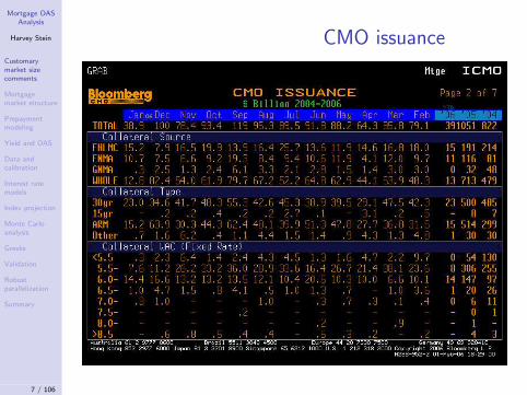
CMO issuance

7 / 106


Harvey Stein



Prepaymentmodeling

Yield and OAS

Data andcalibration

Interest ratemodels

Index projection

Monte Carloanalysis

Greeks

Validation


Summary

Mortgage market structure:

• Mortgages

• MBS pools

• CMOs

8 / 106


Harvey Stein



Prepaymentmodeling

Yield and OAS

Data andcalibration

Interest ratemodels

Index projection

Monte Carloanalysis

Greeks

Validation


Summary

The subatomic particles -mortgages

People take out loans (mortgages) to buy homes.

• Fixed rate mortgages — fixed coupon, monthly payments, selfamortizing, paying principal down to zero at maturity (15-30years).

• Balloons – amortize on a 30 year basis, but expire in 5 or 7 yearswith payment of the remaining outstanding balance.

• Adjustable rate mortgages (ARMS) — floating coupon based onan index (LIBOR, treasury rates, . . . ), typically with protectionclauses against overly large coupon changes (lifetime andperiodic caps, annual resets, . . . ).

Low interest rates in recent years have sparked innovation — floatingrate balloons with interest only payments, various sorts of built inprotections, option ARMs, . . .

9 / 106


Harvey Stein



Prepaymentmodeling

Yield and OAS

Data andcalibration

Interest ratemodels

Index projection

Monte Carloanalysis

Greeks

Validation


Summary

Mortgage behavior

While it looks like ARM valuation might require some work, in thatthey have embedded caps and ratchets and potentially float on aCMS rate, one might think that at least fixed rate mortgages wouldbe easily valued.With fixed monthly payments, monthly interest payments at a rate ofC on the outstanding balance, N monthly payments and an initialbalance of B , then monthly payments are:

C (1 + C )NB

(1 + C )N − 1.

10 / 106


Harvey Stein



Prepaymentmodeling

Yield and OAS

Data andcalibration

Interest ratemodels

Index projection

Monte Carloanalysis

Greeks

Validation


Summary

Mortgage cash flows

Graphically, our cash flows look like:

so why not just discount and be done?

11 / 106


Harvey Stein



Prepaymentmodeling

Yield and OAS

Data andcalibration

Interest ratemodels

Index projection

Monte Carloanalysis

Greeks

Validation


Summary

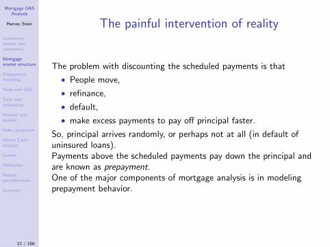
The painful intervention of reality

The problem with discounting the scheduled payments is that

• People move,

• refinance,

• default,

• make excess payments to pay off principal faster.

So, principal arrives randomly, or perhaps not at all (in default ofuninsured loans).Payments above the scheduled payments pay down the principal andare known as prepayment.One of the major components of mortgage analysis is in modelingprepayment behavior.

12 / 106


Harvey Stein



Prepaymentmodeling

Yield and OAS

Data andcalibration

Interest ratemodels

Index projection

Monte Carloanalysis

Greeks

Validation


Summary

Impact of prepayment on cashflows

Thus, our simple mortgage, instead of having fixed cash flows, hascash flows that are dependent on prepayment rates. Under oneprepayment assumption, we have:

13 / 106


Harvey Stein



Prepaymentmodeling

Yield and OAS

Data andcalibration

Interest ratemodels

Index projection

Monte Carloanalysis

Greeks

Validation


Summary

Impact of prepayment on cashflows

Under a model that projects prepayments based on interest rates andloan characteristics, we see a different cash flow structure for eachrate path. One example is:

14 / 106


Harvey Stein



Prepaymentmodeling

Yield and OAS

Data andcalibration

Interest ratemodels

Index projection

Monte Carloanalysis

Greeks

Validation


Summary

The atoms — MBS Pools

In 1938, the collapse of the national housing market led to the federalgovernment’s formation of the Federal National Mortgage

Association, AKA “Fannie Mae”. Now, we have Fannie Mae, FreddieMac (The Federal Home Loan Mortgage Corporation), and GinnieMae The Government National Mortgage Association.

• Banks make mortgages.

• Government insures conforming mortgages.

• Agencies buy conforming mortgages.

• Banks have money to make more mortgages.

• Agencies sell shares of mortgages on secondary market.

Ginnie, Fannie and Freddie — three sets of rules for conforming loans.

15 / 106


Harvey Stein



Prepaymentmodeling

Yield and OAS

Data andcalibration

Interest ratemodels

Index projection

Monte Carloanalysis

Greeks

Validation


Summary

MBS secondary market - poolsThe agencies (Fannie, Freddie and Ginnie) buy mortgages, pool themtogether into MBS pools and sell shares. Pools are pass-throughsecurities, in that the cash flows from the underlying collateral ispassed through to the shareholder, minus a service fee.

16 / 106


Harvey Stein



Prepaymentmodeling

Yield and OAS

Data andcalibration

Interest ratemodels

Index projection

Monte Carloanalysis

Greeks

Validation


Summary

MBS pool fine characteristics -Geographic data

These days, there’s substantial information available about poolcomposition, such as geographic data:

17 / 106


Harvey Stein



Prepaymentmodeling

Yield and OAS

Data andcalibration

Interest ratemodels

Index projection

Monte Carloanalysis

Greeks

Validation


Summary

MBS pool fine characteristics -Loan purpose

18 / 106


Harvey Stein



Prepaymentmodeling

Yield and OAS

Data andcalibration

Interest ratemodels

Index projection

Monte Carloanalysis

Greeks

Validation


Summary

MBS pool fine characteristics -Loan to value ratio and credit

ratings

19 / 106


Harvey Stein



Prepaymentmodeling

Yield and OAS

Data andcalibration

Interest ratemodels

Index projection

Monte Carloanalysis

Greeks

Validation


Summary

MBS pool fine characteristics -loan rate distribution

20 / 106


Harvey Stein



Prepaymentmodeling

Yield and OAS

Data andcalibration

Interest ratemodels

Index projection

Monte Carloanalysis

Greeks

Validation


Summary

MBS pool fine characteristicsLTV distribution

21 / 106


Harvey Stein



Prepaymentmodeling

Yield and OAS

Data andcalibration

Interest ratemodels

Index projection

Monte Carloanalysis

Greeks

Validation


Summary

MBS pool fine characteristicsLoan size distribution

22 / 106


Harvey Stein



Prepaymentmodeling

Yield and OAS

Data andcalibration

Interest ratemodels

Index projection

Monte Carloanalysis

Greeks

Validation


Summary

MBS pool fine characteristicsMaturity distribution

23 / 106


Harvey Stein



Prepaymentmodeling

Yield and OAS

Data andcalibration

Interest ratemodels

Index projection

Monte Carloanalysis

Greeks

Validation


Summary

MBS pool fine characteristicsAge distribution

24 / 106


Harvey Stein



Prepaymentmodeling

Yield and OAS

Data andcalibration

Interest ratemodels

Index projection

Monte Carloanalysis

Greeks

Validation


Summary

MBS pool fine characteristicsCredit rating distribution

25 / 106


Harvey Stein



Prepaymentmodeling

Yield and OAS

Data andcalibration

Interest ratemodels

Index projection

Monte Carloanalysis

Greeks

Validation


Summary

MBS pool fine characteristicsServicers

26 / 106


Harvey Stein



Prepaymentmodeling

Yield and OAS

Data andcalibration

Interest ratemodels

Index projection

Monte Carloanalysis

Greeks

Validation


Summary

MBS pool fine characteristicsSellers

27 / 106


Harvey Stein



Prepaymentmodeling

Yield and OAS

Data andcalibration

Interest ratemodels

Index projection

Monte Carloanalysis

Greeks

Validation


Summary

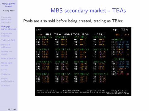
MBS secondary market - TBAs

Pools are also sold before being created, trading as TBAs:

28 / 106


Harvey Stein



Prepaymentmodeling

Yield and OAS

Data andcalibration

Interest ratemodels

Index projection

Monte Carloanalysis

Greeks

Validation


Summary

Pool analysis

Pool analysis is like mortgage analysis, except that it benefits fromsafety in numbers.

• Backed by a substantial number of individual loans, so variance isreduced.

While it used to be the case that this was at the cost of only knowinggross aggregate data about the pool, these days the fine structure ofthe pool is often disclosed as well, telling us:

• Location of individual loans,

• Size of individual loans,

• LTV,

• and credit ratings.

The only thing missing is individual borrower details.

29 / 106


Harvey Stein



Prepaymentmodeling

Yield and OAS

Data andcalibration

Interest ratemodels

Index projection

Monte Carloanalysis

Greeks

Validation


Summary

The molecules — CMOs

In 1983, Solomon Brothers and First Boston created the firstCollateralized Mortgage Obligation (CMO).They realized that more pools could be sold if the pool cash flowswere carved up to stratify risk.CMOs are:

• Backed by pools or directly by mortgages (whole loans),sometimes by as many as 20,000 of them.

• Split up cash flows of underlying collateral into a number of“bonds” or “tranches”.

• By creating desirable risk structures, tranches can be sold to awider audience, and at a profit.

CMOs are essentially arbitrary structured notes backed by mortgagecollateral.

30 / 106


Harvey Stein



Prepaymentmodeling

Yield and OAS

Data andcalibration

Interest ratemodels

Index projection

Monte Carloanalysis

Greeks

Validation


Summary

Tranche types

Tranches vary by how the principal and interest are carved up.

• Interest handling:

• Fixed cpn — Can behave like a pool or very differently,depending on how principal is paid.

• POs — Only principal payments from underlying collateral.• IOs — Only interest payments.• Floaters — Where there’s a floater, there’s an inverse floater(when you have fixed rate collateral).

• Inverse floaters.

• Principal handling:

• Sequential Pay — Sequence of tranches. First gets principal untilpaid, then 2nd gets principal, etc. Last one is most prepaymentprotected and behaves most like an ordinary bond.

• PACs — Scheduled principal will be payed as long as prepaymentremains in a specified band.

• TACs — Scheduled principal will be payed when prepayment is ata specified level.

• Etc.

31 / 106


Harvey Stein



Prepaymentmodeling

Yield and OAS

Data andcalibration

Interest ratemodels

Index projection

Monte Carloanalysis

Greeks

Validation


Summary

Example CMO

32 / 106


Harvey Stein



Prepaymentmodeling

Yield and OAS

Data andcalibration

Interest ratemodels

Index projection

Monte Carloanalysis

Greeks

Validation


Summary

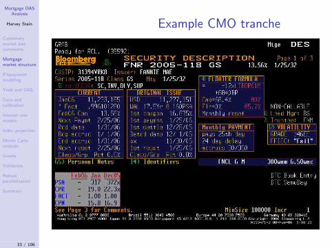
Example CMO tranche

33 / 106


Harvey Stein



Prepaymentmodeling

Yield and OAS

Data andcalibration

Interest ratemodels

Index projection

Monte Carloanalysis

Greeks

Validation


Summary

Example CMO collateral

34 / 106


Harvey Stein



Prepaymentmodeling

Yield and OAS

Data andcalibration

Interest ratemodels

Index projection

Monte Carloanalysis

Greeks

Validation


Summary

CMO modeling

Computing the cash flows of a CMO tranche requires modeling theCMO, i.e. — converting the prospectus into a mathematicalspecification of the tranche payouts as a function of collateral cashflows.

35 / 106


Harvey Stein



Prepaymentmodeling

Yield and OAS

Data andcalibration

Interest ratemodels

Index projection

Monte Carloanalysis

Greeks

Validation


Summary

CMO cash flow engine

The cash flow engine computes CMO cash flows for each scenario.Inputs:

• CMO deal specification.

• Index projections.

• Current outstanding balance of each piece of collateral.

Given the above inputs, the cash flow engine parses and evaluates thedeal specification, using the cash flows generated from running theprepayment model on each piece of collateral and amortizing it.

36 / 106


Harvey Stein



Prepaymentmodeling

Yield and OAS

Data andcalibration

Interest ratemodels

Index projection

Monte Carloanalysis

Greeks

Validation


Summary

Prepayment modeling

37 / 106


Harvey Stein



Prepaymentmodeling

Yield and OAS

Data andcalibration

Interest ratemodels

Index projection

Monte Carloanalysis

Greeks

Validation


Summary

Prepayment speeds

Prepayment speeds are to prepayment modeling what yieldcalculations are to interest rate modeling.

• SMM — Percentage of remaining balance above scheduled paid:

100P′

i −Pi

Bi.

• CPR — SMM annualized: 100(1− (1− SMM

100 )12).

• PSA — “Prepayment Speed Assumption”: 0.2% initially,increasing by 0.2% each month for the first 30 months, and 6.0%until the loan pays off. 200 PSA is double this rate, etc.

• MHP — PSA for manufactured housing (ABS, not MBS).

Looking at the value of a pool or CMO as a function of prepaymentlevel is a useful analysis tool.

38 / 106


Harvey Stein



Prepaymentmodeling

Yield and OAS

Data andcalibration

Interest ratemodels

Index projection

Monte Carloanalysis

Greeks

Validation


Summary

Prepayment speed graph

39 / 106


Harvey Stein



Prepaymentmodeling

Yield and OAS

Data andcalibration

Interest ratemodels

Index projection

Monte Carloanalysis

Greeks

Validation


Summary

Prepayment modeling

Prepayment modeling is a major component of MBS and CMOvaluation. In some sense, CMO and MBS valuation is Monte Carloanalysis of the prepayment model.In prepayment modeling:

• Salient features of prepayment are proposed.

• Evidence is collected statistically.

• Models are developed for these relationships.

40 / 106


Harvey Stein



Prepaymentmodeling

Yield and OAS

Data andcalibration

Interest ratemodels

Index projection

Monte Carloanalysis

Greeks

Validation


Summary

Major prepayment components

• Housing turnover.

• Refinancing.

• Curtailment and Default.

41 / 106


Harvey Stein



Prepaymentmodeling

Yield and OAS

Data andcalibration

Interest ratemodels

Index projection

Monte Carloanalysis

Greeks

Validation


Summary

Housing turnover

• Appears as relatively constant baseline level of prepayment =total (existing) home sales divided by total housing stock.

• Seasonality — Less movement in the winter.

• Seasoning — Chances of moving increase with age of mortgage,but tend to level off. A function of WAM, loan type, andprepayment incentive.

• Lock-in effect — High rates relative to mortgage coupon are adisincentive to moving when LTV is high.

• Rarely over 10% CPR.

42 / 106


Harvey Stein



Prepaymentmodeling

Yield and OAS

Data andcalibration

Interest ratemodels

Index projection

Monte Carloanalysis

Greeks

Validation


Summary

Housing turnover illustrationHousing turnover behavior typically dominates prepayment when ratesare low.

43 / 106


Harvey Stein



Prepaymentmodeling

Yield and OAS

Data andcalibration

Interest ratemodels

Index projection

Monte Carloanalysis

Greeks

Validation


Summary

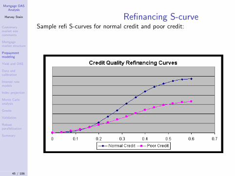
RefinancingRefinancing is the major interest rate dependent component.

• “S-curve” — Zero when rates are above the mortgage coupon,picks up as rates drop and tops out at some maximum level (noteveryone can refinance).

• Aging — New loans less likely to be refinanced due to refi costs,but mitigated by high refi incentive.

• Credit quality — Lower credit quality less likely to refi. Can uselevel of cpn above mortgage rates at issuance in lieu of FICOscore.

• Burnout — As borrowers refinance out of a pool, the remainingborrowers are less likely to refinance (unaware or unable).

• Media effect — Prepayments tend to surge around multi-yearlows, presumably induced by press coverage encouragingrefinancing.

• Pipeline effect — Prepayment rate spikes are asymmetric.Prepayment drops slower than it grew. Due to mortgage brokercapacity limits causing refi applications to back up.

• Lagged effects.

44 / 106


Harvey Stein



Prepaymentmodeling

Yield and OAS

Data andcalibration

Interest ratemodels

Index projection

Monte Carloanalysis

Greeks

Validation


Summary

Refinancing S-curveSample refi S-curves for normal credit and poor credit:

45 / 106


Harvey Stein



Prepaymentmodeling

Yield and OAS

Data andcalibration

Interest ratemodels

Index projection

Monte Carloanalysis

Greeks

Validation


Summary

Curtailment and Default

Default results in return of outstanding principal when property issold.Curtailment is the reduction in maturity due to additional partialpayment of principal. Without reamortization, results in additionalprincipal pay downs on a monthly basis. Can also be from paying offremainder of an old mortgage.

• Tend to be independent of interest rates.

• Default risk grows and then drops as LTV decreases.

• Curtailment picks up towards end of mortgage life.

46 / 106


Harvey Stein



Prepaymentmodeling

Yield and OAS

Data andcalibration

Interest ratemodels

Index projection

Monte Carloanalysis

Greeks

Validation


Summary

Curtailment and Default graphThese considerations lead to the following typical curtailment anddefault graph.

47 / 106


Harvey Stein



Prepaymentmodeling

Yield and OAS

Data andcalibration

Interest ratemodels

Index projection

Monte Carloanalysis

Greeks

Validation


Summary

Loan level characteristics

Increased disclosure allows improved prepayment modeling.Primary loan attributes:

• LTV

• FICO score

• loan size

Secondary loan attributes:

• occupancy

• property type

• loan purpose

48 / 106


Harvey Stein



Prepaymentmodeling

Yield and OAS

Data andcalibration

Interest ratemodels

Index projection

Monte Carloanalysis

Greeks

Validation


Summary

Yield calculations

49 / 106


Harvey Stein



Prepaymentmodeling

Yield and OAS

Data andcalibration

Interest ratemodels

Index projection

Monte Carloanalysis

Greeks

Validation


Summary

Yield calculations

Internal rate of return at a given price assuming a particularprepayment rate.

• Pick a prepayment speed.

• Generate cash flows.

• Solve for internal rate of return that gives quoted price.

Conceptually simple, but computationally intensive and involved whentrying to value a CMO backed by 20,000 pools, with cash flowscarved up across 100 tranches.

50 / 106


Harvey Stein



Prepaymentmodeling

Yield and OAS

Data andcalibration

Interest ratemodels

Index projection

Monte Carloanalysis

Greeks

Validation


Summary

Yield example — PSA

51 / 106


Harvey Stein



Prepaymentmodeling

Yield and OAS

Data andcalibration

Interest ratemodels

Index projection

Monte Carloanalysis

Greeks

Validation


Summary

Yield example — BPM

52 / 106


Harvey Stein



Prepaymentmodeling

Yield and OAS

Data andcalibration

Interest ratemodels

Index projection

Monte Carloanalysis

Greeks

Validation


Summary

OAS Analysis

53 / 106


Harvey Stein



Prepaymentmodeling

Yield and OAS

Data andcalibration

Interest ratemodels

Index projection

Monte Carloanalysis

Greeks

Validation


Summary

From Yield to OASConsider a semi-annual bond with cash flows Ci at times ti (withprincipal payment included in CN) and (dirty) price P . When thebond is not callable, OAS is basically Z-spread, which is basically aspread over a set of bonds which is basically a difference in yields.

P ≈N

∑

1

Ci

(1 + Y2 )

2tiYield

P ≈

N∑

1

Ci

(1 + R+S2 )2ti

Spread

P ≈

N∑

1

Ci

(1 + Yi+S2 )2ti

Z-Spread

P ≈

N∑

1

Ci

(1 + Yi+S2 )2ti

OAS

54 / 106


Harvey Stein



Prepaymentmodeling

Yield and OAS

Data andcalibration

Interest ratemodels

Index projection

Monte Carloanalysis

Greeks

Validation


Summary

Optionality in OASWhen the bond has embedded optionality, OAS attempts to value theoptionality. Doing this requires some assumptions regarding theevolution of interest rates:

55 / 106


Harvey Stein



Prepaymentmodeling

Yield and OAS

Data andcalibration

Interest ratemodels

Index projection

Monte Carloanalysis

Greeks

Validation


Summary

MBS and CMO OASCompute average value under a large set of realistic scenarios. TheOAS is the shift in the discount rates needed to arrive at a specifiedprice.Because of the complexity and path dependency of the prepaymentmodel and the CMO tranche calculations, OAS analysis is done viaMonte Carlo.

• Calibrate interest rate model.

• Generate interest rate scenarios — discount rates, longer tenorrates, par rates.

• Generate indices — current coupons, district 11 cost of funds,and whatever else is needed.

• For each scenario:

• Compute prepayments for each piece of collateral.• Amortize each piece of collateral.• Compute tranche cash flows.• Discount cash flows at specified OAS to generate scenario price.

• Average of scenario prices is the price at the specified OAS.

56 / 106


Harvey Stein



Prepaymentmodeling

Yield and OAS

Data andcalibration

Interest ratemodels

Index projection

Monte Carloanalysis

Greeks

Validation


Summary

Data and calibration

57 / 106


Harvey Stein



Prepaymentmodeling

Yield and OAS

Data andcalibration

Interest ratemodels

Index projection

Monte Carloanalysis

Greeks

Validation


Summary

Data importance

Data:

• Most critical component of interest rate modeling.

• Weak model calibrated to good data is far better than a strongmodel calibrated to the wrong data.

• Data must have good pricing and capture risks of securities beingvalued.

• Characterizing risk in terms of related liquid instruments will helpto answer the question of which interest rate model to use.

58 / 106


Harvey Stein



Prepaymentmodeling

Yield and OAS

Data andcalibration

Interest ratemodels

Index projection

Monte Carloanalysis

Greeks

Validation


Summary

Discounting componentTraditionally, the treasury curve. Thought to be closest in risk toagency default risk (i.e. negligible), but:

• Heterogeneous — coupon bonds, some liquid and some illiquid.

• Sparse data — large gaps between maturities leaves interimpricing unknown (subject to interpolation method).

• Market price of conditional cash flows (i.e. option prices =Volatility data) unavailable.

Newer market standard — calibrate to the swap curve.

• Denser data — monthly at short end, annually further out. Lesssubject to interpretation.

• Homogeneous — cash rates and par rates, not bond prices atvarying coupons. Mostly on a clean, nominal basis.

• Rich volatility data — ATM and OTM caps and floors are wellknown. ATM swaptions of various tenors and maturities are wellknown. Only OTM swaption pricing is subject to discussion.

• Hedging — swap market often used to hedge MBSs. Calibratingto it makes calculating appropriate hedges easier.

59 / 106


Harvey Stein



Prepaymentmodeling

Yield and OAS

Data andcalibration

Interest ratemodels

Index projection

Monte Carloanalysis

Greeks

Validation


Summary

Volatility calibration

What to calibrate to?

• Calibrate to full volatility cube? Too expensive to hedge.

• Calibrate to one volatility? Which one?

Compromise 1: Two year and ten year swaptions are commonly usedfor hedging, so calibrate to them.Compromise 2: Rather than calibrating to the entire smile, calibrateto the ATMs and pick a model which does a reasonable job ofcapturing the overall smile. This is also good because OTM swaptiondata is hard to come by.

60 / 106


Harvey Stein



Prepaymentmodeling

Yield and OAS

Data andcalibration

Interest ratemodels

Index projection

Monte Carloanalysis

Greeks

Validation


Summary

Interest rate models

61 / 106


Harvey Stein



Prepaymentmodeling

Yield and OAS

Data andcalibration

Interest ratemodels

Index projection

Monte Carloanalysis

Greeks

Validation


Summary

Popular short rate models

Log normal short rate models have been popular for many years in thefixed income markets.

• Simple and intuitive.

• A priori, rates shouldn’t go negative.

62 / 106


Harvey Stein



Prepaymentmodeling

Yield and OAS

Data andcalibration

Interest ratemodels

Index projection

Monte Carloanalysis

Greeks

Validation


Summary

A log normal short rate model(LNMR)

One example is the first model we used for mortgage valuation. Theshort rate process is rt , where:

rt = eRt+θt

dRt = −aRtdt + σdWt ,

with a and σ constants, θt is a function of time and chosen tocalibrate the model to the discount curve. Under this model Rt is aGaussian process mean reverting to zero, and rt is log normal andmean reverting as well.

63 / 106


Harvey Stein



Prepaymentmodeling

Yield and OAS

Data andcalibration

Interest ratemodels

Index projection

Monte Carloanalysis

Greeks

Validation


Summary

Drawbacks of 1 factor LNMR

• Model skew is flat in log normal terms, which is not what’sobserved in the market today.

• Correlated rates.

• Calibration rigidity — can calibrate to the yield curve and twooption prices. Mean reversion is known to be hard to calibrate.However, greater flexibility can be introduced with timedependent volatility (Black-Derman-Toy).

64 / 106


Harvey Stein



Prepaymentmodeling

Yield and OAS

Data andcalibration

Interest ratemodels

Index projection

Monte Carloanalysis

Greeks

Validation


Summary

US skews 1 year outIt always pays to look at the data. Here are cap and swaption impliedvolatilities from the US market. The skew is substantial acrossmaturities.

0

5

10

15

20

25

30

35

40

45

-5 -4 -3 -2 -1 0 1 2 3 4

1y2y1y5y1y10y1y caplet (CFIR)1y caplet (ICPL)

65 / 106


Harvey Stein



Prepaymentmodeling

Yield and OAS

Data andcalibration

Interest ratemodels

Index projection

Monte Carloanalysis

Greeks

Validation


Summary

US skews 5 years outThe five year tenors are skewed as well.

0

5

10

15

20

25

30

35

40

45

-5 -4 -3 -2 -1 0 1 2 3 4

5y2y5y5y5y10y5y caplet (CFIR)5y caplet (ICPL)

66 / 106


Harvey Stein



Prepaymentmodeling

Yield and OAS

Data andcalibration

Interest ratemodels

Index projection

Monte Carloanalysis

Greeks

Validation


Summary

How normal is it?Fitting the CEV model (dr = σrβdW ) to caplet skews shows that theUS market is fairly close to normal (β close to zero).

0

0.2

0.4

0.6

0.8

1

1.2

0 5 10 15 20 25 30 35

USDEURJPY

67 / 106


Harvey Stein



Prepaymentmodeling

Yield and OAS

Data andcalibration

Interest ratemodels

Index projection

Monte Carloanalysis

Greeks

Validation


Summary

How normal is it?Fitting errors for the CEV model to the US market aren’t too large, soabove betas are reasonable.

0%2%4%6%8%

10%12%14%

0 2 4 6 8 10 12

USDEURJPY

68 / 106


Harvey Stein



Prepaymentmodeling

Yield and OAS

Data andcalibration

Interest ratemodels

Index projection

Monte Carloanalysis

Greeks

Validation


Summary

LGM

The Linear Gaussian Markovian models (AKA Hull-White models) area family of extremely tractable models. The two factor form is:

rt = θt + Xt + Yt

dXt = −aXXtdt + σX (t)dW1

dYt = −aY Ytdt + σY (t)dW2

dW1dW2 = ρdt

69 / 106


Harvey Stein



Prepaymentmodeling

Yield and OAS

Data andcalibration

Interest ratemodels

Index projection

Monte Carloanalysis

Greeks

Validation


Summary

LGM advantages

• Fits overall historical behavior well with fixed mean reversion andcorrelation (ax = 0.03, ay = 0.5, ρ = −0.7).

• Can be calibrated to two term structures of volatility.

• Very tractable — Don’t underestimate the value of closed formsolutions (or decent approximations) for bond prices, capletprices,and swaption prices and swap rates as a function of(Xt ,Yt).

• Much closer to market skew than log normal models.

70 / 106


Harvey Stein



Prepaymentmodeling

Yield and OAS

Data andcalibration

Interest ratemodels

Index projection

Monte Carloanalysis

Greeks

Validation


Summary

LGM behavior

• High mean reversion factor dampens long term effect of thatparameter, leaving long tenor volatility mostly determined by lowmean reversion factor.

• Both factors impact short tenor volatility.

• Negative correlation reduces volatility of short maturities relativeto long maturities and allows this behavior to persist in time.

71 / 106


Harvey Stein



Prepaymentmodeling

Yield and OAS

Data andcalibration

Interest ratemodels

Index projection

Monte Carloanalysis

Greeks

Validation


Summary

Market volatility term structure

0 20 40 60 80 100 12016

17

18

19

20

21

22

23

24

Bla

ck S

wap

tion

Vol

s (%

)

Swaption expiries (months)

1−year2−year3−year4−year5−year7−year10−year

Swaption term structure — implied volatilities as a function ofmaturity for various tenors.

72 / 106


Harvey Stein



Prepaymentmodeling

Yield and OAS

Data andcalibration

Interest ratemodels

Index projection

Monte Carloanalysis

Greeks

Validation


Summary

LGM volatility term structure

0 20 40 60 80 100 12015

16

17

18

19

20

21

22

23

24

Bla

ck S

wap

tion

Vol

s (%

)

Swaption expiries (months)

1−year2−year3−year4−year5−year7−year10−year

LGM model’s swaption term structure — implied volatilities producedby the model, as a function of maturity for various tenors.

73 / 106


Harvey Stein



Prepaymentmodeling

Yield and OAS

Data andcalibration

Interest ratemodels

Index projection

Monte Carloanalysis

Greeks

Validation


Summary

Index projection

74 / 106


Harvey Stein



Prepaymentmodeling

Yield and OAS

Data andcalibration

Interest ratemodels

Index projection

Monte Carloanalysis

Greeks

Validation


Summary

Index projection problem

• Prepayment model needs appropriate inputs (such as monthlymortgage refi rates).

• Floater indices (such as D11COFI) need to modeled.

• Neither need be discount rates, and hence, can’t be read directlyfrom model.

75 / 106


Harvey Stein



Prepaymentmodeling

Yield and OAS

Data andcalibration

Interest ratemodels

Index projection

Monte Carloanalysis

Greeks

Validation


Summary

Index projection solutions

• Not a problem for discount rates (LIBOR, swap rates, etc).Compute from model:

• For one factor log normal — build lattice and compute futureimplied long tenor rates for each month as a function of the shortrate.

• For 2 factor LGM — rates are given by formulas.

• Avoid problem — calibrate prepayment model directly todiscount rates (LIBOR, swap rates, etc).

• Simplify — to first order can ignore volatility of index relative todiscount rates. How different can refi rates be on two differentdates that have the same swap curve? Regress and model as afunction of the rates. Or get fancy and take vol into account aswell.

76 / 106


Harvey Stein



Prepaymentmodeling

Yield and OAS

Data andcalibration

Interest ratemodels

Index projection

Monte Carloanalysis

Greeks

Validation


Summary

Chosen solution

We chose simple:

• Treat implied rates as a function of swap rates.

• Regress — proxy the current coupon for each collateral type as aweighted average of the 2 year and 10 year rates.

• Adjust for current actual value of current coupons.

• Adjust in prepayment model for fact that a proxy for the refi rateis being used.

• Potentially use lagged data (e.g. - D11COFI in ARM Wrestling:

Valuing Adjustable Rate Mortgages Indexed to the Eleventh

District Cost of Funds, by Stanton and Wallace.

77 / 106


Harvey Stein



Prepaymentmodeling

Yield and OAS

Data andcalibration

Interest ratemodels

Index projection

Monte Carloanalysis

Greeks

Validation


Summary

Monte Carlo analysis

78 / 106


Harvey Stein



Prepaymentmodeling

Yield and OAS

Data andcalibration

Interest ratemodels

Index projection

Monte Carloanalysis

Greeks

Validation


Summary

The need for speed

With 20,000 pieces of collateral, interpreted rules for paying out cashflows and time consuming prepayment projection calculations, runningthe 100,000 scenarios necessary for accurate valuation will take sometime. If a scenario takes 0.0001 seconds on one piece of collateral,then we’ll have to wait 2.3 days. 100 scenarios would take 3.3minutes.So, it pays to reduce the number of scenarios needed.

79 / 106


Harvey Stein



Prepaymentmodeling

Yield and OAS

Data andcalibration

Interest ratemodels

Index projection

Monte Carloanalysis

Greeks

Validation


Summary

1 factor pseudo Monte Carlo

In the one factor case, the method we developed is the bifurcationtree approach.

• Begin with two paths starting at the current short rate.

• Evolve them to match the moments of the model relative to thelast common point.

• Periodically allow the paths to split:

Ru = E[Rt|Rb = R] +√

Var[Rt|Rb = R]

Rd = E[Rt|Rb = R]−√

Var[Rt|Rb = R]

80 / 106


Harvey Stein



Prepaymentmodeling

Yield and OAS

Data andcalibration

Interest ratemodels

Index projection

Monte Carloanalysis

Greeks

Validation


Summary

1 factor LNMR

E[Rt|Rb = R] and Var[Rt|Rb = R] can be computed from the SDEfor Rt by using eat as an integrating factor, yielding:

Rt = ea(b−t)Rb +

∫ t

b

σea(s−t)dWs ,

soE[Rt|Rb] = Rbe

−a(t−b),

and

Var[Rt|Rb] =σ2

2a(1− e

−2a(t−b)).

81 / 106


Harvey Stein



Prepaymentmodeling

Yield and OAS

Data andcalibration

Interest ratemodels

Index projection

Monte Carloanalysis

Greeks

Validation


Summary

1 factor pseudo Monte Carlo

The end result, with 5 selected bifurcation maturities, is the followingtree:

82 / 106


Harvey Stein



Prepaymentmodeling

Yield and OAS

Data andcalibration

Interest ratemodels

Index projection

Monte Carloanalysis

Greeks

Validation


Summary

Bifurcation tree behavior

Advantages:

• Reasonably straight forward.

• Conditional mean and variance of underlying R process ismatched at bifurcation points.

• Results look reasonable with fairly small numbers of paths.

Disadvantages:

• Variability is coarse (semiannual steps).

• Unclear that overall variance is captured.

• Doesn’t extend well to the multi-factor case.

83 / 106


Harvey Stein



Prepaymentmodeling

Yield and OAS

Data andcalibration

Interest ratemodels

Index projection

Monte Carloanalysis

Greeks

Validation


Summary

LGM — VR1 — Numeraireconsiderations

We’ve investigated a variety of variance reduction techniques for the 2factor LGM model.The first is to recognize that the choice of numeraire has a majorimpact on Monte Carlo efficiency.Consider valuation of a price process V under two differentnumeraires N and N ′, and corresponding equivalent Martingalemeasures Q and Q ′.

V0 = N0EQ [

Vt

Nt

] = N ′0EQ′

[Vt

N ′t]

84 / 106


Harvey Stein



Prepaymentmodeling

Yield and OAS

Data andcalibration

Interest ratemodels

Index projection

Monte Carloanalysis

Greeks

Validation


Summary


The relationship between N, N ′, Q and Q ′ is that

N/N0

N ′/N0=

dQ

dQ ′,

where dQ/dQ ′ is the Radon-Nikodym derivative of Q with respect toQ ′.So, a numeraire that’s higher on high rates will have an equivalentMartingale measure that’s correspondingly higher as well, and thusthe Monte Carlo associated with the higher numeraire will samplemore heavily from this region.

85 / 106


Harvey Stein



Prepaymentmodeling

Yield and OAS

Data andcalibration

Interest ratemodels

Index projection

Monte Carloanalysis

Greeks

Validation


Summary


MBS gross behavior:

• High rates — Low prepayment — MBS behavior becomes morestable.

• Low rates — High prepayment — MBS behavior moreinteresting.

Numeraire selection — Choose numeraire that’s low for high ratesand high for low rates:

• Integrated form of LGM is very convenient — simplifies formulas.But, numeraire is low for low rate paths, causing poor MonteCarlo behavior.

• Standard money market numeraire is much better. Harder towork with, but does better importance sampling.

86 / 106


Harvey Stein



Prepaymentmodeling

Yield and OAS

Data andcalibration

Interest ratemodels

Index projection

Monte Carloanalysis

Greeks

Validation


Summary

LGM — VR2 — path shifting

Adjust paths so that sample at least captures yield curve.

• Similar to doing control variate on the discount rates.

• rt = θt + Xt + Yt , and Xt and Yt are Gaussian and symmetricaround zero, so just compute a new θ to get discounting correctfor chosen path set.

VR1 + VR2 yields pricing standard deviation of about 1bp for 2,000paths, or ≤ 1 bp error ≈ 30% of the time, and ≤ 2 bp error ≈ 66% ofthe time.

87 / 106


Harvey Stein



Prepaymentmodeling

Yield and OAS

Data andcalibration

Interest ratemodels

Index projection

Monte Carloanalysis

Greeks

Validation


Summary

LGM — VR3 — PCA

• Randomly sample paths P = (Xt1 , . . .Xtn ,Yt1 , . . .Ytn)

• Xti and Yti are jointly distributed as a 2n dimensional Gaussianwith zero mean.

• Let C be the covariance matrix of these 2n random variables.

• If Z = (z1, ..., z2n)t), and the zi are IID N(0, 1), and C = AAt ,

then AZ has the same distribution as P .

• Choose A to be the matrix whose columns are the eigenvectorsof C , scaled by the square roots of their eigenvalues. ThenC = AAt .

• The best k factor approximation to P is given by using the firstk columns of V .

• Small number of vectors capture most of variance.

• In 1 factor LGM — 7 vectors out of 360 for 95% of variance.

• In 2 factor LGM — 9 vectors out of 720 for 95% of variance.

88 / 106


Harvey Stein



Prepaymentmodeling

Yield and OAS

Data andcalibration

Interest ratemodels

Index projection

Monte Carloanalysis

Greeks

Validation


Summary

LGM — VR4 — Weighted PCA

• Most of action in pool is up front, both because of prepaymentand because of discounting.

• Weight PCA with e−αt to effect this.

• Weight two factors differently as well (High MR factor doesn’thave as big an impact on MBS pricing as low MR factor).

89 / 106


Harvey Stein



Prepaymentmodeling

Yield and OAS

Data andcalibration

Interest ratemodels

Index projection

Monte Carloanalysis

Greeks

Validation


Summary

LGM — VR5 — Local antitheticsampling

• Pure antithetic just makes sure sample mean is correct.

• Not so effective in interest rate MC.

• Do local antithetic instead (”uniform sampling with antitheticnoise” (UWAN)) - Dupire and Savine:

• Build a grid.• Pick antithetic pairs from each box.• Uses MC to eliminate convexity caused bias.

• Done on first few eigenvectors.

90 / 106


Harvey Stein



Prepaymentmodeling

Yield and OAS

Data andcalibration

Interest ratemodels

Index projection

Monte Carloanalysis

Greeks

Validation


Summary

LGM — VR1+VR2+VR4+VR5 —Weighted PCA with local

antithetic sampling

Combine methods:

• VR1 — Money market numeraire.

• VR2 — Path shifting.

• VR4 — Weighted PCA.

• VR5 — Local antithetic sampling.

VR1+VR2+VR4+VR5 = standard deviation of 300 paths is lowerthan 5000 for VR1+VR2.

91 / 106


Harvey Stein



Prepaymentmodeling

Yield and OAS

Data andcalibration

Interest ratemodels

Index projection

Monte Carloanalysis

Greeks

Validation


Summary

LGM — VR1+VR2+VR4 withSobol sequences

Adding Sobol sequences to the mix:

• Use Sobol sequences to randomly scale eigenvectors.

• Further reduces variance.

92 / 106


Harvey Stein



Prepaymentmodeling

Yield and OAS

Data andcalibration

Interest ratemodels

Index projection

Monte Carloanalysis

Greeks

Validation


Summary

Results

128 256 512 1024 2048 40960.0001

0.0002

0.0003

0.0006

0.0011

0.002

0.0037

Number of Paths

RM

SE

FWDPC UWAN1PC UWAN2PC UWAN3PC SobolWPC UWAN1WPC UWAN2WPC UWAN3WPC Sobol

93 / 106


Harvey Stein



Prepaymentmodeling

Yield and OAS

Data andcalibration

Interest ratemodels

Index projection

Monte Carloanalysis

Greeks

Validation


Summary

Greeks

94 / 106


Harvey Stein



Prepaymentmodeling

Yield and OAS

Data andcalibration

Interest ratemodels

Index projection

Monte Carloanalysis

Greeks

Validation


Summary

Greek errors

Greeks magnify pricing errors.

dP

dS≈

P(S + h)− P(S − h)

2h

If P(S) is the true model price, and P̃(S) is what we compute, thenthe error is ε(S) = P̃(S)− P(S).

P̃(S + h)− P̃(S − h)

2h=

P(S + h) + ε(S + h)− (P(S − h) + ε(S − h))

2h

=∆P/2h +∆ε/2h

2

= dP/dS +d3P/dS3

3!h2 + . . .+∆ε/2h

So, the error in the calculation is the error from dropping the higherorder terms and from the change in error with respect to S .

95 / 106


Harvey Stein



Prepaymentmodeling

Yield and OAS

Data andcalibration

Interest ratemodels

Index projection

Monte Carloanalysis

Greeks

Validation


Summary

Greek errors

Errors in derivative are caused by:

• High order terms corrupting finite difference (“convexity”).

• Pricing error.

Error control:

• Small h reduces Greek error from convexity.

• Large h reduces Greek error from pricing error.

Pricing error issues:

• Finite difference — ε flat, minimal problems.

• Monte Carlo — ε large and random — error goes to ∞ as h → 0.

Solution for Monte Carlo:

• Make ε less random — Use the same paths, or the same randomnumber seed.

• Accurate duration with 25bp shift, even when pricing variance isas large as 6bp.

96 / 106


Harvey Stein



Prepaymentmodeling

Yield and OAS

Data andcalibration

Interest ratemodels

Index projection

Monte Carloanalysis

Greeks

Validation


Summary

Which Greeks?

To compute duration, rates are shifted while other inputs are heldconstant. How should the option data be held constant?

• Hold prices constant — Doesn’t make sense. Option prices haveto change as rates make them more or less in the money.

• Hold vol constant — Vol is a log normal vol, but LGM model isnormal. If vol is held constant, then model volatility will changewhen the rates are shifted.

• Hold normal vol constant — Most consistent with LGM model.

The situation between normal vol and log normal vol is reversed forthe LNMR model.

97 / 106


Harvey Stein



Prepaymentmodeling

Yield and OAS

Data andcalibration

Interest ratemodels

Index projection

Monte Carloanalysis

Greeks

Validation


Summary

Validation

98 / 106


Harvey Stein



Prepaymentmodeling

Yield and OAS

Data andcalibration

Interest ratemodels

Index projection

Monte Carloanalysis

Greeks

Validation


Summary

Validation

How to make sure entire process works?General methods:

• Results are stable over time. Jumps can be explained byoccurrence of a change in the market.

• Fitted parameters stable over time as well.

• Prices and OASs behave appropriately

• Flat in neighborhood of current cpn.• Expected relationships between different securities hold.• Prices and OASs move as expected when input parameters arechanged:

• Yield curve shifts.• Volatility shifts.• Shifts of current index values.

Mortgage specific:

• Compare to empirical durations.

99 / 106


Harvey Stein



Prepaymentmodeling

Yield and OAS

Data andcalibration

Interest ratemodels

Index projection

Monte Carloanalysis

Greeks

Validation


Summary

Robust parallelization

100 / 106


Harvey Stein



Prepaymentmodeling

Yield and OAS

Data andcalibration

Interest ratemodels

Index projection

Monte Carloanalysis

Greeks

Validation


Summary

Parallelization

Variance reduction alone is insufficient to compute OASs in real time.Need parallelization

• Linux clusters.

• 6 clusters, 50 dual CPU PCs each = 100 CPUs per cluster

• Embarrassingly parallel sometimes isn’t

• Communication costs to farm out results and get back can renderparallelization useless.

• Old cluster - 750mhz, 100mbps ethernet — 60 seconds, 6 inparallel.

• New cluster - 3.0ghz, 100mbps ethernet — 15 seconds, 4 secondsin parallel.

• Data dissemination problem — 2 gb of deal and collateralspecifications.

• PCA parallelization — compute time vs communication speed.

101 / 106


Harvey Stein



Prepaymentmodeling

Yield and OAS

Data andcalibration

Interest ratemodels

Index projection

Monte Carloanalysis

Greeks

Validation


Summary

Request flow

• User hits <go>

• Computation data is assembled:

• current values• user selected values.

• request sent to dispatcher

• dispatcher queues until an idle server is available. Retries failedrequests.

• Server receives request.

• Explodes base calculation into individual path requests

• farms them out across the cluster

• redundancy and robustness

• assembles the result

• farms out remaining requests

• assembles results

• replies to client.

102 / 106


Harvey Stein



Prepaymentmodeling

Yield and OAS

Data andcalibration

Interest ratemodels

Index projection

Monte Carloanalysis

Greeks

Validation


Summary

Data dissemination

How to keep 2gb current on 300 machines?

• Layered approach.

• Source keeps head machines up to date.

• Head machines update remainder of cluster.

• Distribute within cluster in a tree fashion:

• Copy from head to 4 children.• Each time a node is updated, it starts updating 4 new nodes, andits updater starts updating a new node.

• Utilizes full bandwidth of ethernet switch — 100mbps from eachmachine to switch, but independent pairs of machines cansustain this up until the switch’s backplane capacity.

103 / 106


Harvey Stein



Prepaymentmodeling

Yield and OAS

Data andcalibration

Interest ratemodels

Index projection

Monte Carloanalysis

Greeks

Validation


Summary

Parallelization robustness

Preventing machine problems from causing calculation failures.Errors encountered:

• Unstripable curves.

• Overheating machines.

• Flakey hard disks.

• Data unavailable.

• Bad data supplied.

Layered approach:

• Requests -> dispatcher -> OAS server -> slaves.

• If dispatcher gets an error (on a full request), it resends (up tothe retry limit).

• If OAS server gets an error (on a path), it marks the slave as badand tries again. If it gets confirmation of the error, the slave ismarked good and the path is listed as bad. If not, the slave is nolonger used.

104 / 106


Harvey Stein



Prepaymentmodeling

Yield and OAS

Data andcalibration

Interest ratemodels

Index projection

Monte Carloanalysis

Greeks

Validation


Summary

Parallelization issues

Even embarrassingly parallel problems might have troubleparallelizing.

• Even the simplest variance reduction adds up startup costs andcommunication overhead.

• If startup costs can’t be distributed as well, then they yield ahard limit on parallelization speedup.

• PCA analysis is slow enough that it’s hard to make it actuallysave time.

• Compression of data being distributed.• Tree distribution of data.• Optimize PCA.• Parallelize PCA.• Partial PCA.

105 / 106


Harvey Stein



Prepaymentmodeling

Yield and OAS

Data andcalibration

Interest ratemodels

Index projection

Monte Carloanalysis

Greeks

Validation


Summary

SummaryCMO valuation is big science — lots of moving parts, with each onedrawing on a different area:

• Prepayment modeling:• Statistical validation and modeling of economic and behavioralanalysis.

• Data selection:• Risk analysis.

• Interest rate modeling:• Classic arbitrage pricing theory.

• Index projection:• Statistical analysis.

• Monte Carlo analysis:• Numerical methods.• Variance reduction techniques.

• Parallelization:• Building computation clusters.• Analysis and optimization of parallel algorithms.

As Emanuel Derman says, the best quants are interdisciplinarians.CMO valuation is one area that requires it.

106 / 106

Mortgage OAS Harvey Stein...

Documents

Transcript of Mortgage OAS Harvey Stein...