Morphology and Charge Transport in P3HT: A Theorist’s …andrienk/publications/poelk… · ·...

Adv Polym SciDOI: 10.1007/12_2014_277© Springer-Verlag Berlin Heidelberg 2014

Morphology and Charge Transport in P3HT:

A Theorist’s Perspective

Carl Poelking, Kostas Daoulas, Alessandro Troisi, and Denis Andrienko

Abstract Poly(3-hexylthiophene) (P3HT) is the fruit fly among polymeric organic

semiconductors. It has complex self-assembling and electronic properties and yet

lacks the synthetic challenges that characterize advanced donor–acceptor-type poly-

mers. P3HT can be used both in solar cells and in field-effect transistors. Its morpho-

logical, conductive, and optical properties have been characterized in detail using

virtually any and every experimental technique available, whereas the contributions

of theory and simulation to a rationalization of these properties have so far been

modest. The purpose of this review is to take a snapshot of these results and, more

importantly, outline directions that still require substantial method development.

Keywords Charge transport � Conjugated polymers � Morphology � Organic

semiconductors � P3HT � Simulation

Contents

1 Introduction

2 Morphology

2.1 Single Molecules

2.2 Crystalline Oligothiophenes

2.3 Amorphous Melts and Blends

C. Poelking and D. Andrienko (*)

Max Planck Institute for Polymer Research, Ackermannweg 10, 55128 Mainz, Germany

e-mail: [email protected]; [email protected]

K. Daoulas

Max Planck Institute for Polymer Research, Ackermannweg 10, 55128 Mainz, Germany

InnovationLab GmbH, 69115 Heidelberg, Germany

e-mail: [email protected]

A. Troisi

Department of Chemistry and Centre for Scientific Computing, University of Warwick,

Coventry CV4 7AL, UK

e-mail: [email protected]

mailto:[email protected]




3 Coarse-Grained Models

3.1 Structure-Based Coarse-Graining

3.2 Soft Models

4 Rate-Based Description of Charge Transport

4.1 Rates

4.2 Reorganization Energy

4.3 Electronic Coupling Elements

4.4 Site Energies

4.5 Charge Mobility

4.6 Autocorrelation of Electronic Couplings and Site Energies

5 First-Principles-Based Calculations for Large Models of Polymer

5.1 The Charge Localization–Length Problem

5.2 Strategies for Large-Scale Electronic-Structure Calculations of Polymer Models

5.3 Results from the Computation of the Wavefunction for Large-Scale Polymer Models

6 Outlook

References

1 Introduction

Thiophene-based conjugated polymers have accompanied, if not originated, the

interest in conductive polymer materials and their application in organic field-effect

transistors (OFETs) and organic photovoltaic (OPV) devices [1]. The most studied

representative of this class of materials is poly(3-hexyl-thiophene) (P3HT) with its

regioregular (head-to-tail) isomer (see Fig. 1), as first synthesized by Rick

McCullough in 1992 [2]. Polythiophenes, however, were already an intensely

studied class of conjugated polymers, a rudimentary description of the compound

being published as early as 1883 [3]. The first polymerization reactions with high

yield and small concentrations of synthesis impurities were reported in 1980

[4, 5]. These compounds were essentially not processable due to the strong inter-

action of the conjugated backbones. In 1986, Elsenbaumer reported the synthesis of

easily processable poly(alkyl-thiophenes) (PATs) [6]. Solution-processed into thin

films, these materials could exhibit reasonable conductivities limited, however, by

the disorder that results from a regiorandom attachment of the side chains to the

thiophene monomers. It was the synthesis of regioregular (rr) P3ATs [2] that

eventually paved the way for applications in devices such as OFETs and OPV

cells. Here, we recapitulate key experimental results relevant to polymorphism,

formation of self-assembled nanostructures, and charge transport in rr-P3HT. An

extended overview is provided in the rest of the contributions of this volume,

various books, and monographs (e.g., [7])

Like many conjugated polymers, P3HT is a polymorph, i.e., forms different

crystal structures depending on processing conditions. The most frequently

observed are so-called forms I and II [8], which differ by the side chain conforma-

tion and interdigitation, inclination of conjugated backbones with respect to the

stacking direction, and the shift of successive (along the π-stacking direction)

polymer chains [9]. Form I, which is observed after annealing, is the structure

encountered in most studies dealing with OFETs and OPVs. It has a monoclinic

C. Poelking et al.

unit-cell (for bulk P3HT samples X-ray diffraction, XRD, provides a¼ 1.60 nm,

b¼ 0.78 nm, and c¼ 0.78 nm [10]). Polymorph II has been found to have a

significantly smaller unit cell dimension along the a-axis and has thus been assumed

to have interdigitated alkyl groups [8], which distinguishes it from form I. Upon

heating, form II irreversibly transforms into form I. This phase transition is accom-

panied by a change in unit-cell dimensions, with interlayer spacings increasing and

intrastack distances decreasing. A similar first-order phase transition has been

described recently in a combined infrared-spectroscopy and wide-angle XRD

study for a non-interdigitated metastable polymorph that transforms into the stable

form I, hence establishing a third polymorph, I0 [11, 12]. Simulated unit cells of

polymorphs I and I0 are shown in Fig. 2.

On a mesoscale, crystallization from supercooled solutions in poor solvents can

lead to the formation of secondary structures, notably nanofibers, with a width of

tens of nanometers and length of several micrometers [14].

Charge transport in P3HT has been studied with the aim of relating

regioregularity, molecular weight and, hence, morphology to hole mobility, and

thus to the efficiency of P3HT/methanofullerene (PCBM) bulk heterojunction solar

cells, for which the power conversion efficiency was reported to be 4.4% as early as

2005 [15]. Hole mobilities of 10�5 cm2/V s (10�4 cm2/V s) were measured for 94%

(98%) regioregular P3HT using the time-of-flight (TOF) technique [16]. Dispersive

transients of the regiorandom P3HT indicated that the polymer is conductive, yet its

mobility could not be extracted from TOF measurements due to sizeable disorder.

The mobility temperature dependence, analyzed using the Gaussian disorder model

(GDM), suggested an energetic disorder of around 50–60 meV. Both hole and

electron TOF mobilities were reported to be independent of the molecular weight

up to 20 kDa, and then decreased by an order of magnitude as molecular weight

increased to 120 kDa [17]. The reported zero-field mobilities for shorter chains

were of the order of 10�4 cm2/V s. A GDM-fitted energetic disorder of 71(54)meV

was extracted for short (long) chains.

Meanwhile, field-effect mobilities ranging around μ ~10�5 cm2/V s were

reported for the very first OFET device that used polythiophene for the semicon-

ducting channel [18]. By choosing rr-P3HT, μ could be increased by three orders of

magnitude [19]. OFET mobilities of ~0.1 cm2/V s were measured as a function of

the molecular weight after spin-casting from higher boiling point solvents [20]. The

field-effect mobility was found to increase with molecular weight in spite of

reduced crystallinity. This was attributed to either better interconnectivity of the

Fig. 1 Regioregular poly

(3-alkyl-thiophene) (P3HT)

Morphology and Charge Transport in P3HT: A Theorist’s Perspective

polymer network [21] or smaller intrachain ring torsions present in high molecular

weight molecules [22].

Transistor hole mobilities have even been reported for individual P3HT

nanofibers [14, 23, 24]. Along the fiber, this mobility was as high as 0.06 cm2/V s.

An energetic disorder of 108 meV was extracted from temperature-dependent

measurements.

Stimulated by this multitude of experimental investigations, a number of theo-

retical studies have been conducted to rationalize the wide spectrum of mobilities

obtained for a single compound and link the transport characteristics to the self-

assembly properties, morphology, and electronic structure of P3HT. The contro-

versy started when examining conformations of a single isolated chain: the thio-

phene dimer was reported to adopt a twisted backbone conformation [25], whereas

increasing the oligomer length resulted in a planarized backbone. The situation with

oligomer assemblies is even more involved; indeed, we still do not know the order

of crystalline polymorphs on the energy axis, cannot quantify the density of defects

in a crystalline morphology, or quantify the relative volume fractions of crystalline

and amorphous phases. We do not really understand what exactly limits charge

transport in ordered lamellar systems: is it large energetic disorder or small elec-

tronic couplings? Why is the hole transport strongly dispersive even though the

reported energetic disorder is moderate? How does regioregularity contribute to

morphological ordering, density of states, and electronic couplings? In which ways

does molecular weight impact mobility? Our goal is to summarize approaches and

answers to some of these questions from a theoretical perspective and to provide an

outlook for the remaining questions.

a b

α = β = 90◦

γ = 86.17◦

a = 15.09 A

b = 8.06 Ac = 7.89 A

a = 16.18 A

γ = 86.16◦α = β = 90◦

b = 7.72 Ac = 7.89 A

b

2c 2c

a

b

a

polymorph I, CA-100polymorph I’,CC-100

Fig. 2 Unit cells of polymorphs I0 (a) and I (b) as obtained from molecular dynamics simulations.

To highlight the backbone and side chain packing, we use C for crystalline and A for amorphous

states, i.e., CA-100 corresponds to a system with a crystalline arrangement of backbones, amor-

phous packing of side-chains, and regioregularity of 100%. CC-100 corresponds to a system with

crystalline side chains and 100% regioregularity. Adapted with permission from Poelking

et al. [13]. Copyright (2013) American Chemical Society

C. Poelking et al.

2 Morphology

The theoretical and computational toolbox used to study self-assembling properties

of conjugated polymers is very versatile: On the highest level of resolution, it

includes accurate quantum chemical calculations capable of predicting the proper-

ties of isolated oligomers and dimers, normally without side chains. Less compu-

tationally demanding density functional methods can deal with much longer

oligomers (10–20 repeat units), including side chains, and are often used to

compare ground state energies of experimentally proposed arrangements of atoms

in a unit cell. To assess crystalline packing modes at ambient conditions and during

annealing, as well as to study amorphous melts and longer chain lengths, classical

force fields have been parametrized. To access even longer length and time scales

(micrometers, microseconds), coarse-grained models have been developed to study

amorphous melts and liquid-crystalline phases of P3HT.

The ultimate goal of these simulations is to self-assemble the polymer in silico,

i.e., to predict its polymorphs as well as the degree of disorder in the kinetically

trapped molecular arrangements. The honest assessment is that we are fairly far

from achieving this goal. The main obstacles are insufficient accuracy of methods at

a specific level of resolution, long simulation times required to study self-assembly,

and uncontrolled error propagation from one level to another, e.g., when parame-

terizing force fields based on quantum chemical calculations, or developing coarse-

grained models using force-field-generated reference data.

We will provide a summary of simulation results, starting with single-molecule

properties and then expanding to molecular arrangements of P3HT in crystals,

melts, and finally binary mixtures with PCBM, a typical acceptor used in organic

solar cells.

2.1 Single Molecules

Ab initio methods have been extensively used to analyze conformations of the

conjugated backbone and side-chain orientations with respect to the plane of

conjugation [25]. Here, the extended π-conjugated system flattens the backbone,

whereas nonbonded interactions between consecutive repeat units (i.e., steric

repulsions between hydrogen atoms, Coulomb interactions, and van der Waals

interactions) often tend to distort its planarity. For P3HT, both planar [26] and

nonplanar stable geometries have been reported, depending on the side-chain

orientation [27]. At the B3LYP/6-31+G level of density functional theory (DFT),

the nonplanar backbone has an energy of ~0.03 eV lower (per monomer) than the

planar backbone (evaluated in a 10-mer) [28]. This indicates that chain conforma-

tions in the bulk are predominantly determined by interchain van der Waals and

Coulomb interactions, a conclusion also drawn from calculations of molecular

dimers [29].


Because typical energy differences between planar and nonplanar conformations

are in the order of tens of millielectronvolts, which is the accuracy threshold of

density functional methods, one is forced to use more accurate (and computation-

ally demanding) quantum-chemical methods. However, the ground-state twist

angle between repeat units has been found to depend on the oligomer length,

saturating at about ten repeat units. Furthermore, torsional potentials are correlated

up to the second-nearest-neighbor rings [30], thus making geometry predictions a

formidable task even for isolated oligomers [31].

2.2 Crystalline Oligothiophenes

Both density functional and force-field calculations have been used to study

crystalline P3HT mesophases. Density functional calculations have been primarily

used to establish whether experimentally reported crystal structures correspond to

well-defined energy minima [32–35]. Using a van-der-Waals-corrected generalized

gradient approximation (GGA) functional, Dag and Wang concluded that the

crystal with shifted backbones (i.e., with one of the thiophene layers shifted along

the chain direction by the thiophene–thiophene distance) and side chains rotated

around the torsion angle is the most stable of three studied structures [36]. Xie

et al. reached the conclusion that a structural motif without this registry shift and

without rotation of the side chains, but instead with a small backbone tilt, has the

lowest potential energy [34]. Similar to the situation with a single isolated chain,

typical energy differences between different packing motives are in the order of

10 meV per unit cell and, hence, theoretical methods are at their accuracy limits,

making it difficult to rank different molecular arrangements. Also, unit-cell opti-

mizations are performed at zero Kelvin, meaning that entropic effects, notably the

chain excluded volume, are ignored.

To study larger systems and longer timescales, various flavors of P3HT force

fields were developed. In the majority of cases, parameters of an existing force field

were refined in order to reproduce the torsional potential between thiophene units

and electrostatic potential around an isolated oligomer [13, 37]. The parametriza-

tion has been subsequently refined to account for the change in the backbone

potential with oligomer length [13, 26, 28, 38–40]. To this end, atomistic simula-

tions have been used to analyze proposed packing arrangements of three P3HT

polymorphs (phases I, I0, and II; see Fig. 2), and to scrutinize the effect of

regioregularity on paracrystalline, dynamic, and static nematic order parameters

[13]. Molecular dynamics simulations suggest that the most stable P3HT poly-

morph has planar thiophene backbones shifted by one thiophene ring with respect to

each other. Hexyl side chains are twisted away from the backbone in a transfashion, resulting in a non-interdigitated packing structure, although stable struc-

tures with interdigitated side chains were also reported [41]. Force-field-based

estimates of the mass density (1.05 g cm�3), melting temperature (490 K), and

surface tension (32 mN/m) all agree with the reported experimental values

C. Poelking et al.

[40]. One should note that even on this classical level of description, only highly

crystalline morphologies and high-temperature amorphous melts can be studied.

Still, some indications of local-chain ordering upon cooling of amorphous high-

temperature melts (see Fig. 3) have been observed [42].

2.3 Amorphous Melts and Blends

Early simulations of amorphous systems considered thiophene oligomers as a

model for P3HT. Alignment of polymer chains and thiophene units within chains

have for instance been studied in a Monte-Carlo approach [43]. The authors were

able to reproduce the density of the amorphous mesophase (an estimate of

1.06 g cm�3 was given) and concluded that chains tend to align parallel to each

other, while thiophene rings of neighboring chains tend to adopt parallel or anti-

parallel π-stacked arrangements. Systems with much shorter chains had signifi-

cantly denser packing (predicted density 1.4 g cm�3) and stronger alignment, a

result obtained using molecular dynamics simulations [44].

Amorphous melts of oligomers of P3HT were also simulated in order to calcu-

late the glass transition temperature (300 K) and, hence, validate the atomistic force

field [40] and to develop coarse-grained models of P3HT in a liquid state

approaching 500–600 K [45, 46]. Simulations of free-standing films of P3HT

melts have been used to estimate the room-temperature value of surface tension

(21–36 mN m�1) [47]. Amorphous melts of P3HT are, however, of only moderate

interest because the conductive abilities of this polymer are related to its high

degree of lamellar ordering.

Fig. 3 Typical configuration of the amorphous system after annealing the crystal at high temper-

atures (left). Onset of crystallization at 300 K acquired at the end of the gradual cooling process

that was started from the amorphous melt (right). Adapted with permission from Alexiadis and

Mavrantzas [42]. Copyright (2013) American Chemical Society


In order to understand molecular ordering and electronic processes in bulk

heterojunction devices, blends of P3HT oligomers with fullerene and PCBM have

been simulated at different levels of resolution. Atomistic simulations showed that

bulk oligothiophenes (five chains of 20 repeat units each) tend to cluster better than

oligothiophene/fullerene systems [48]. Prototypical model interfaces have been

used to evaluate energetic profiles for electrons and holes [49]. Coarse-grained

simulations could observe the onset of phase separation [45], distributions of

domain sizes, and interface-to-volume ratios [50] in P3HT/PCBM mixtures. Nev-

ertheless, the field of coarse-grained modeling of conjugated polymers is still in its

infancy. Complications reside in the large persistence length and anisotropic

nonbonded interactions that promote π–π stacking. We will discuss various strate-

gies for developing coarse-grained models of conjugated polymers in Sect. 3.

3 Coarse-Grained Models

Apart from the local molecular packing discussed so far, mesoscopic ordering of

conjugated polymers is equally important for the functionality of organic semicon-

ducting devices. In a bulk heterojunction solar cell, for example, domain sizes of

the donor and acceptor mesophases have considerable impact on cell efficiency. To

predict and analyze such effects, modeling strategies that target the morphology on

length scales reaching several hundreds of nanometers, the typical thickness of the

active layer in a polymer-based solar cell, are required. With the currently available

computational power, such system sizes can only be addressed on a coarse-grained

level.

The idea of coarse-graining relies on the separation of time and length scales.

For many polymeric systems, especially polymer melts, the chemical details,

although strongly affecting material behavior on the microscopic level, become

less important on the mesoscale, where simplified representations of polymer

architecture and interactions can be used. In conjugated polymers, however, the

mesoscale features of the morphology couple across many length scales: π–πstacking for instance promotes the formation of lamellae, which in turn self-

assemble into supralamellar structures. Predicting this hierarchical self-assembly

is the main target (and challenge) of coarse-grained modeling of conjugated

polymers.

Coarse-graining strategies can be subdivided into bottom-up and top-down

approaches [51, 52]. In bottom-up coarse-graining, the model is constructed to

reproduce physical quantities known from a more detailed description of the system

[53]. In other words, a fine-grained representation of the system is projected onto a

representation with fewer degrees of freedom. This projection is not unique, and

various techniques have been suggested, including structure-based coarse-graining

[53, 54], force-matching [55, 56], and relative entropy frameworks [57]. Top-down

C. Poelking et al.

approaches, on the contrary, derive the coarse-grained model from macroscopic

observables (e.g., the phase behavior). These are often based on experimental

measurements [51, 52, 58] but can also incorporate elements of bottom-up

coarse-graining. In the following sections, we review the results obtained using

structure-based coarse-grained models and also introduce a coarse-graining tech-

nique based on soft interaction potentials.

3.1 Structure-Based Coarse-Graining

The idea of structure-based coarse-graining is to match structural properties, such

as radial distribution functions, of the fine- and coarse-grained systems. Structure-

based coarse-grained models have been developed for melts [45, 46], high-

temperature (liquid) mixtures of P3HT/PCBM [45, 50, 59], and solutions of

P3HT [60]. The P3HT monomers are normally coarse-grained into three interaction

sites placed at the center of mass of the thiophene rings, then on the first and last

three methyl groups of the hexyl side-chain, as shown in Fig. 4. The bonded and

nonbonded interaction parameters are optimized using the iterative Boltzmann

inversion method [54, 61], although phenomenological refinement is also used [59].

The three-site models allow for self-assembling polymer backbones into lamel-

lar arrangements [59, 60]. They have also been used to study the morphology of

phase-separated P3HT/PCBM blends, where explicit incorporation of side chains

helped to understand penetration of acceptor molecules into side chains as a

function of their grafting density along the backbone. No intercalation was found

for P3HT, in contrast to poly(bithiophene-alt-thienothiophene) (PBTTT), which

has a lower grafting density of side chains [59]. A further advantage of coarse-

graining is that solvent-mediated interactions can be incorporated into coarse-

grained interactions, leading to a dramatic decrease in the number of degrees of

freedom. Simulations of P3HT aggregation in solutions with anisole could repro-

duce the experimentally observed aggregation of P3HT as a function of temperature

with the back-folded hairpins of stacked P3HT molecules [60]. The spacing

between P3HT lamellae was found to be 1.7 nm, which is comparable to experi-

mental observations [9].

Three-site coarse-grained models normally employ orientationally isotropicnonbonded interactions and are parametrized either on high-temperature P3HT

melts or solutions. Thus, by construction, they cannot capture the directionality of

π–π interactions between thiophenes. The backbones of the P3HT chains within the

same lamella are also less correlated, leading to smectic-like ordering [59, 60]. In

fact, this type of ordering has been reported experimentally, although in a narrow

temperature window, prior to melting [10].


3.2 Soft Models

The three-site models with explicit beads for side chains are too complex for

simulations of dense systems and long chains. For homopolymer melts, oligomers

of 15 repeat units have been used [59], whereas simulations of P3HT/PCBM blends

employed chains of 48 repeat units [45]. Further reducing the number of degrees of

freedom, e.g., by removing coarse-grained side chains, necessitates orientationally

anisotropic interaction potentials, otherwise even the lamellar order is no longer

produced. In other words, anisotropic interactions are needed to account for the

conformational frustration of side chains and the energetically favorable stacking of

backbones. In this sense, they incorporate entropic and enthalpic contributions to

the free energy of the system.

As the model becomes cruder and cruder, the number of microscopic states that

correspond to the same coarse-grained state increases. As a result, the coarse-

grained interaction potentials become softer. This, in combination with the reduc-

tion in the degrees of freedom, boosts computational efficiency. At the same time,

the thermodynamic nature of the coarse-grained potentials becomes more promi-

nent and transferability is gradually lost [62]. To remedy the situation, thermody-

namic properties of the system can be incorporated into the coarse-grained model

by using (phenomenological) top-down approaches. For conjugated polymers, the

symmetry of the mesophase can be directly included into the anisotropic interaction

potential, as has been shown for liquid crystalline mesophases [63, 64] observed

experimentally in poly[3-(20-ethyl)hexylthiophene] and poly(3-dodecylthiophene)

[65, 66].

In such coarse-grained models, nonbonded interactions are chosen such that the

system possesses a desired phase behavior, e.g., a nematic to isotropic transition.

In practice, one starts with an appropriate density functional, in the spirit of

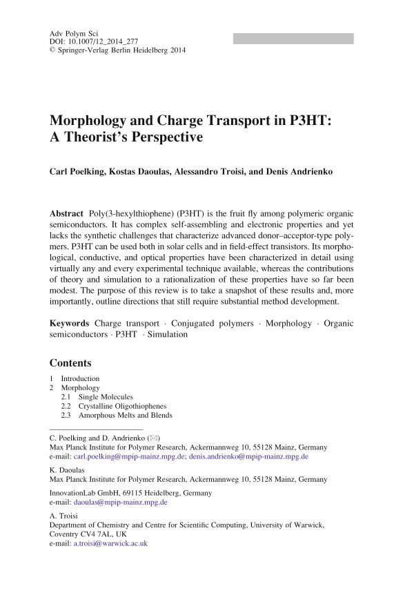
Fig. 4 Left: Three-sitecoarse-grained model of

polythiophene derivatives

with different side chain

grafting densities. Right:PCBM modeled by a

collection of 13 coarse-

grained beads. Bead types

are labeled by letters A

(buckyball), B (backbone),

and S (side chain). Adapted

with permission from

Jankowski et al. [59].

Copyright (2013) American

Chemical Society

C. Poelking et al.

field-theoretical descriptions of polymeric liquid crystals [67–71]. Each s-th coarse-grained thiophene of the i-th molecule with coordinate ri(s) is assigned an ortho-

normal set of vectors {nð1Þi (s), n

ð2Þi (s), n

ð3Þi (s)} as illustrated in Fig. 5. A repeat unit is

smeared into a density distribution ω(r� ri(s)), which allows for collective degreesof freedom:

ρ rð Þ ¼Xni¼1

XNs¼1

ω r� ri sð Þð Þ

Q αβ rð Þ ¼ ρ�10

Xni¼1

XNs¼1

ω r� ri sð Þð Þqi,αβ sð Þ

B αβ rð Þ ¼ ρ�10

Xni¼1

XNs¼1

ω r� ri sð Þð Þbi,αβ sð Þ

ð1Þ

where α, β¼ x, y, z, and

qi,αβ sð Þ ¼ 3

2n

1ð Þi,α sð Þn 1ð Þ

i,β sð Þ � δαβ2

�"ð2Þ

bi,αβ sð Þ ¼ n2ð Þi,α sð Þn 2ð Þ

i,β sð Þ � n3ð Þi,α sð Þ, n 3ð Þ

i,β sð Þh i

ð3Þ

are the orientational order parameters. The density cloud ω(r� ri(s)) represents, tosome extent, the distribution of the underlying microscopic degrees of freedom

[72]. Because molecules in a nematic phase are orientationally ordered but posi-

tionally disordered and side chain conformations strongly fluctuate, the average

spatial distribution of monomers can be approximated by a spherical uniform

density cloud, ω rð Þ ¼ 34 πσ3

if r� σ, zero otherwise. For P3HT, for example,

σ¼ 0.6 nm, which is close to the length of a hexyl chain in the all-trans configu-ration, ~0.76 nm.

s − 1

θ

s

s + 1

n(1)(s)

n(3)(s)n(2)(s)

φ

Fig. 5 Atomistic and coarse-grained representation of a P3HT chain (left), including

coarse-grained angular (θ) and dihedral (ϕ) degrees of freedom (center). Biaxial nematic alignment

in a melt of P3HT chains (right). Adapted with permission from Gemunden et al. [64]. Copyright

(2013) American Chemical Society


The nonbonded interactions are then defined through a free-energy functional of

the collective variables [64]:

Hnm ; ρ ; Q ; Bh i

¼ðdr

κ ρ02

ρ rð Þρ0

� 1

0@

1A

2

� ν ρ03

ðdrQ rð Þ : Q �

r�

� μ ρ03

ðdr�Q rð Þ : B �

r�þ B

�r�: Q

�r��

� λ ρ04

ðdrB rð Þ : B rð Þ

ð4Þ

Here the first term suppresses local density fluctuations [73, 74] and the rest is an

analog of the Ginzburg–Landau free energy associated with the instantaneous

tensorial fields Q and B . Phenomenological parameters ν, μ and λ entering this

functional are normally chosen such that the thermodynamic state of interest, e.g., a

biaxial–nematic mesophase, is reproduced. In this respect, mean-field estimates can

help to limit the physically adequate parameter ranges. Positive isothermal com-

pressibility, for example, requires κ > νþ μþ λ [64].Following similar studies with scalar collective degrees of freedom [51, 75], one

can then write the effective Hamiltonian of nonbonded interactions as:

Hnb ¼ 1

2

Xni, j¼1

XNs, t¼1

u rij s; tð Þ� �κ � 2ν

3qi sð Þ : qj tð Þ�

24

� 2μ

3

�qi sð Þ : bj

�t�þ bi

�s�: qj

�t�� λ

2bi�s�: bj sð Þ

� ð5Þ

where u(rij(s, t))¼ ρ� 10

Ðdrω(|r� ri(s)|)ω(|r� rj(t)|) is the soft repulsion core

expressing the overlap of the density clouds [51, 64]:

u rij s; tð Þ� � ¼ 3

8πρ0σ32þ rij s; tð Þ

2σ

� �1� rij s; tð Þ

2σ

� �2

ð6Þ

Thus, the free-energy functional is transformed into a sum over pairwise,

orientation-dependent interactions. Note that bonded interaction potentials are

taken into account separately and can be parametrized using atomistic simulations

of a single isolated chain in θ–solvent conditions. Here bond lengths are kept fixed

and harmonic angular and Ryckaert–Bellemans torsion potentials are used to

reproduce the corresponding distributions [64].

C. Poelking et al.

Once the Hamiltonian is fully parametrized, standard sampling techniques

(e.g. Monte Carlo, molecular dynamics, or dissipative particle dynamics) can be

used to explore the phase space and to evaluate macroscopic observables. Note that

the coarse-grained hexylthiophenes interact even at a distance of 2σ¼ 1.2 nm,

which is almost twice the average separation of their centers of mass, estimated

as ρ� 1=30 � 0.63 nm. In order to obtain realistic values for the effective excluded

volume, the interactions for strong overlaps of the density clouds must be weak, i.e.,

κu 0ð Þ � kBT. This results in soft potentials and boosts the efficiency of phase-spacesampling, especially if the Monte Carlo algorithm is used.

Simulations using the reptation algorithm [76, 77] showed that one can equili-

brate systems on the scale of �50� 50� 50 nm3, containing around 5� 10�5

hexylthiophenes with up to 32 monomers per chain. Depending on the coupling

strength λ and the degree of polymerization, plate-like nematic mesophases (with

normals of the thiophene rings parallel to the director) as well as biaxial phases (see

Fig. 5 for a representative snapshot) have been observed. It has also been shown that

the model predicts reasonable values for the persistence length and Frank elastic

constants [64].

With the large-scale morphology at hand, some insights can be obtained on how

the collective orientation of chains affects the energetic landscape for drift-

diffusing charges. This has been done by splitting polymer segments onto conju-

gated segments (using a simple criterion for the torsion angle [78]; see, however,

Sect. 5.1) and evaluating gas-phase ionization energies of these segments. Even this

crude model predicts that isotropic melts consist of short conjugated segments with

defects uniformly distributed along the chains. In the biaxial nematic case, the

average segment length increases significantly, and the collective orientation of

these segments leads to a spatially correlated energetic landscape, even without

accounting for long-range Coulomb interactions [64].

4 Rate-Based Description of Charge Transport

We will now discuss the semiconducting properties of P3HT. When choosing an

appropriate model for charge transport in this polymer, we have to rely on the

experimentally observed increase in mobility with increasing temperature. This is

interpreted as a sign for temperature-activated hopping transport. In other words,

charges (charged states) are localized and charge transfer reactions that propagate

the localized states are thermally activated. Localization can occur on single

molecules (typically observed in amorphous small-molecule-based organic semi-

conductors) or molecular assemblies (crystalline materials). In polymers, charge

localizes on molecular, or conjugated, segments, as discussed in Sect. 5.1.

If charge transfer rates are known, the resulting master equation for occupation

probabilities of these localized states describes charge dynamics in the system.

Hence, the solution of the master equation provides information about charge


distribution, currents, and eventually mobility, all as a function of temperature,

external field, charge density, and, importantly, morphology. Here we will start

with the charge transfer rate and introduce microscopic quantities that affect charge

dynamics.

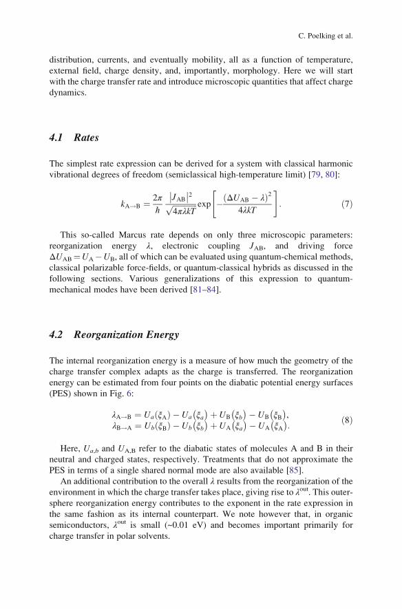
4.1 Rates

The simplest rate expression can be derived for a system with classical harmonic

vibrational degrees of freedom (semiclassical high-temperature limit) [79, 80]:

kA!B ¼ 2π

ℏ

JAB2ffiffiffiffiffiffiffiffiffiffiffiffiffi4πλkT

p exp � ΔUAB � λð Þ24λkT

�:

"ð7Þ

This so-called Marcus rate depends on only three microscopic parameters:

reorganization energy λ, electronic coupling JAB, and driving force

ΔUAB¼UA�UB, all of which can be evaluated using quantum-chemical methods,

classical polarizable force-fields, or quantum-classical hybrids as discussed in the

following sections. Various generalizations of this expression to quantum-

mechanical modes have been derived [81–84].

4.2 Reorganization Energy

The internal reorganization energy is a measure of how much the geometry of the

charge transfer complex adapts as the charge is transferred. The reorganization

energy can be estimated from four points on the diabatic potential energy surfaces

(PES) shown in Fig. 6:

λA!B ¼ Ua ξAð Þ � Ua

�ξa�þ UB

�ξb�� UB

�ξB�,

λB!A ¼ Ub ξBð Þ � Ub

�ξb�þ UA

�ξa�� UA

�ξA

�:

ð8Þ

Here, Ua,b and UA,B refer to the diabatic states of molecules A and B in their

neutral and charged states, respectively. Treatments that do not approximate the

PES in terms of a single shared normal mode are also available [85].

An additional contribution to the overall λ results from the reorganization of the

environment in which the charge transfer takes place, giving rise to λout. This outer-sphere reorganization energy contributes to the exponent in the rate expression in

the same fashion as its internal counterpart. We note however that, in organic

semiconductors, λout is small (~0.01 eV) and becomes important primarily for

charge transfer in polar solvents.

C. Poelking et al.

For P3HT, the reorganization energy decreases to ~0.1 eV for a chain length of

20 monomers, which is small compared to ~0.2–0.4 eV observed in many small-

molecule-based organic semiconductors due to better delocalization of the charge.

Additionally, steric hindrance prevents conformational changes of the polymer

chain upon charging if embedded in a π-stacked crystal. The resulting constraint

on the backbone planarity helps lower the reorganization energy.

4.3 Electronic Coupling Elements

Electronic coupling elements, or transfer integrals, between molecules i and j aregiven by the off-diagonal matrix elements [80, 86]:

Jij ¼ ϕi

Hϕj

� �, ð9Þ

where ϕi,j are diabatic states, often approximated by the frontier orbitals of the

molecules, and H is the dimer Hamiltonian. These quantities are normally evaluated

using electronic structure methods. Expanding the adiabatic states of the dimer in

monomer states, we obtain the following secular equation:

H� ESð ÞC ¼ 0, ð10Þ

where H and S are the Hamiltonian and overlap matrices of the system:

Fig. 6 Diabatic (solid black line) and adiabatic (dashed red line) potential energy surfaces of twoelectronic dimer states |ϕAbi and |ϕaBi participating in the charge transfer reaction along the

reaction coordinate ξ. Reorganization energies λA!B, λB!A


H ¼ ei Hij

H�ij ej

� �, S ¼ 1 Sij

S�ij 1,

� �ð11Þ

and ei ¼ ϕi

Hϕi

� �, ej ¼ ϕj

Hϕj

� �, Hij ¼ ϕi

Hϕj

� �, and Sij¼hϕi|,ϕji

In the basis of its eigenfunctions, the Hamiltonian operator is diagonal,

hϕDn |H|ϕD

mi¼Enδnm. Hence, Eq. (10) can be rewritten as:

Hij ¼Xn

ϕi

ϕDn

� �En ϕD

n

ϕj

� �: ð12Þ

Expanding the monomer and dimer functions into a basis set of atom-centered

orbitals, |ϕki¼∑ αMðkÞα |φαi, |ϕD

n i¼∑ αDðnÞα |φαi, the projections read:

ϕk

ϕDn

� � ¼ Xα

M kð Þα α

� Xβ

Dnð Þβ

βi ¼ M{kð ÞSD nð Þ ð13Þ

where S is the overlap matrix of the atomic basis functions. The Hamiltonian and

overlap then take the form:

Hij ¼ M{ið ÞSDED

{S{M jð Þ ð14ÞSij ¼ M

{ið ÞSDD

{S{M jð Þ ð15Þ

The final required transformation is the diagonalization of the diabatic states

imposed by the charge-transfer Hamiltonian [87]. An orthonormal basis set that

retains the local character of the monomer orbitals can be obtained by using the

Lodwin transformation, Heff¼ S� 1/2HS� 1/2, yielding an effective Hamiltonian

with entries directly related to site energies εi and transfer integrals Jij:

Heff ¼ εi JijJ�ij εj

� �: ð16Þ

The projection method can be significantly simplified if semi-empirical methods

are used for the dimer Hamiltonian [88–90] and made computationally more

efficient by avoiding self-consistent dimer calculations [91].

4.3.1 Crystalline P3HT Couplings

As an illustration, we review the distribution of electronic couplings in P3HT

crystals, molecular-dynamics snapshots of which are shown in Fig. 2. The diabatic

states are constructed from the highest occupied molecular orbital of an optimized

(B3LYP functional, 6-311 g(d,p) basis set) P3HT 20-mer. We account for the

variation in dihedral angles along the polymer backbone by rotating the orbitals

C. Poelking et al.

into the respective coordinate frames of the thiophenes. The electronic coupling

elements are calculated for each molecular pair (ij) from the neighbor list using the

semi-empirical ZINDO method [88–90]. A pair of molecules is added to the list of

neighbors if the distance between the centers-of-mass of any of the thiophene

groups is below a cut-off of 0.5 nm. This small, fragment-based cut-off ensures

that only nearest neighbors are added to the neighbor list.

The distribution of electronic coupling elements is shown in Fig. 7. Note that we

use CA to denote crystalline (amorphous) packing, i.e., CA-100 corresponds to a

system with a crystalline arrangement of backbones, amorphous packing of side-

chains, and regioregularity of 100%. Unexpectedly, the 100% regioregular P3HT

with crystalline side chains (CC-100) has (on average) lower electronic couplings

than the corresponding 90% regioregular phase (CC-90). This peculiar effect is

most probably due to the different interlevel shift observed for the two regioregu-

larities. Transfer integrals tend to be very sensitive to this structural mode [92]. For

two perfectly aligned and optimized chains, the coupling element |Jij|2 can vary

between 0 and 10�2 eV as the backbones are shifted with respect to each other along

the polymer’s long axis by one repeat unit, thus yielding a sin2-type variation of

|Jij|2 with interlevel shift.

Side-chain melting leads to a broadening of the distributions and a tail of very

small couplings, down to 10�6 eV (even though only nearest neighbors are present

in the neighbor list). This would obviously result in rather small average mobility

values [93]. This conclusion is, however, valid only if (one-dimensional) charge-

carrier transport were to occur within a static snapshot of the system; in reality, both

transfer integrals and site energies are time-dependent. In order to understand

whether such a static picture can be used in the case of P3HT, we compare the

distributions of relaxation times of the electronic coupling elements and site

energies to the distribution of escape times of a charge carrier (see Sect. 4.6).

Fig. 7 Distributions of

squared electronic

couplings for CC-100,

CA-100, CC-90, and

CA-90. CA-100corresponds to a system

with a crystalline

arrangement of backbones,

amorphous packing of side-

chains, and regioregularity

of 100%. CC-100corresponds to a system

with crystalline side chains

and 100% regioregularity.

Adapted with permission

from Poelking

et al. [13]. Copyright (2013)

American Chemical Society


4.4 Site Energies

The driving force, ΔUAB, is given by the difference in site energy UA�UB, i.e., the

energy separation between the diabatic PES minima shown in Fig. 6. UA and UB

include both internal contributions Uint, i.e., the electron affinities for electrons and

ionization potentials for holes of isolated molecules, and external contributions

from the electrostatic (U est) and induction (Uind) interactions with surrounding

molecules:

UA ¼ UAb ξAbð Þ � Uab

�ξab

� ¼¼ Uint

Ab � Uintab

� �þ �U est

Ab � U estab

�þ �U ind

Ab � U indab

�UB ¼ UaB ξaBð Þ � Uab

�ξab

� ¼¼ Uint

aB � Uintab

� �þ �U est

aB � U estab

�þ �U ind

aB � U indab

�ð17Þ

Here, the subscript ab denotes the reference (neutral) state of the system, with all

molecules in their ground states.

4.4.1 Electrostatic Contribution

The electrostatic interaction energy in the site-energy calculation can be evaluated

as the first-order energy correction term that results when treating an external field

as a perturbing term in the molecular Hamiltonian. This term is normally evaluated

using atomic distributed multipoles, where the interaction energy UAB of two

molecules A and B, located at positions X and Y reads:

UAB ¼ 1

4πε0

ððd3xd3y

ρA xð ÞρB yð ÞYþ y� X� xj j : ð18Þ

Here ρA and ρB are the charge densities of molecules A and B, respectively.

Using the spherical-harmonic addition theorem [94], this energy can be

rewritten in terms of the molecular multipole moments defined with respect to the

molecule’s local frame:

UAB ¼ 1

4πε0

Xl1, l2

Xk1, k2

l1 þ l2

l1

� �Q A

l1k1Q B

l2k2�

�Sk1k2l1l2l1þl2

X� Y�l1�l2�1 ð19Þ

C. Poelking et al.

These moments, Q Alm ¼

ðd3xρA xð ÞRlm xð Þ, interact with each other via a tensor

that contains the distance and orientation dependence. Note that here we have used

|x� y|< |X�Y| (i.e., the molecular charge densities must not interpenetrate). In

this expression, the so-called S-function [95] has absorbed the orientation depen-

dence, comprising a linear combination of products of Wigner rotation matrices and

3j-coefficients: The latter result from re-centering the spherical harmonics in the

expansion around the molecular centers X and Y.

Due to the spherical-tensor formalism, the molecular multipole moments can be

easily converted between two coordinate frames Σ1 and Σ2 according to

QΣ1ð Þ

lk ¼X

mQ

Σ2ð Þlk Dl

mk φ; θ;ψð Þ. Here, ϕ, θ,ψ are Euler angles and [Dlmk] is a

Wigner rotation matrix. This conversion allows us to perform the electrostatic

parametrization of a molecule within a conveniently chosen local frame, and to

include the transformation from the local to the global interaction frame in a tensor

that takes care of both the distance and orientation dependence:

TA,Bl1k1l2k2

¼ 1

4πε0

l1 þ l2l1

� �Sk1k2l1l2l1þl2

X� Y�l1�l2�1 ð20Þ

This way, the interaction energy reduces to a compact expression, comprising

only molecular multipole moments defined with respect to the molecular local

frame and generic interaction tensors TA,Bl1k1l2k2

(tabulated up to l1 + l2¼ 5 in [96]):

UAB ¼ Q Al1k1

TA,Bl1k1l2k2

Q Bl2k2

, ð21Þ

where we have used the Einstein sum convention for the multipole-moment com-

ponents liki. The site-energy correction that enters exponentially in the Marcus rate

expression for a charge localized on molecule A is then:

ΔU cmA ¼

XB 6¼A

Q A,cl1k1

� Q A,nl1k1

�TA,Bl1k1l2k2

Q B,nl2k2

, ð22Þ

where superscripts c and n denote the molecular multipole moments in the neutral

and charged states, respectively, and the sum runs over all external molecules B.

4.4.2 Distributed Multipoles

In Eq. (21), we have given an expression for the electrostatic interaction energy in

terms of molecule-centered multipole moments. To arrive at this expression, we

required the separation between the molecular centers, |X�Y|, to be larger than the

separation of any of the respective charge-carrying volume elements of the two

molecules, |x� y|. In a molecular solid, this demand can hardly be satisfied,


considering the dense packing and (also important) strongly anisotropic charge

density. This inevitably leads to breakdown of the single-point expansion at small

interseparations. It is possible to avoid this breakdown by choosing multiple

expansion sites (“polar sites”) per molecule in such a way as to accurately represent

the molecular electrostatic potential, with a set of suitably chosen multipole

moments {Qalk} allocated to each site. We then simply extend the expression for

the interaction energy between two molecules A and B in the single-point expan-

sion, Eq. (21), and include the sum over expansion sites a ∈ A and b ∈ B:

UAB ¼Xa∈A

Xb∈B

Q al1k1

Ta,bl1k1l2k2

Q bl2k2

Q al1k1

Ta,bl1k1l2k2

Q bl2k2

, ð23Þ

where we have used the Einstein sum convention for the site indices a and b on the

right-hand side of the equation, in addition to the sum convention that is already in

place for the multipole-moment components.

There are a number of strategies for arriving at such a collection of distributed

multipoles [94, 97–101]. They can be classified according to whether the multipoles

are derived from the electrostatic potential generated by the self-consistent field

(SCF) charge density or from a decomposition of the wavefunction itself. For

example, the CHELPG (charges from electrostatic potentials, grid-based) method

relies on performing a least-squares fit of atom-placed charges to reproduce the

electrostatic potential as evaluated from the SCF density on a regularly spaced grid

[98, 102]. The distributed-multipole-analysis (DMA) approach [99, 100], devel-

oped by A. Stone, operates directly on the quantum-mechanical density matrix,

expanded in terms of atom- and bond-centered Gaussian functions.

4.4.3 Induction Interaction

Similar to the distributed-multipole expansion of molecular electrostatic fields, one

can derive a distributed-polarizability expansion of the molecular field response.

We can start by including the multipole-expansion in the perturbing Hamiltonian

term W ¼ Q at ϕ

at , where we again use the Einstein sum convention for both

superscripts a, referencing an expansion site, and subscripts t, which summarize

the multipole components (l, k) in just one index. Using this approximation for the

intermolecular electrostatic interaction, the second-order energy correction now

reads:

W 2ð Þ ¼ �Xn 6¼0

0h Q at ϕ

at

ni2Wn �W0

: ð24Þ

C. Poelking et al.

We absorb the quantum-mechanical response into a set of intramolecular site–

site polarizabilites, where �αaa0

tt0 ϕa0t0 yields the induced multipole moment Qa

t at site

a that results from a field component ϕa0t0 at site a

0 [94]:

αaa0

tt0 ϕa0t0 ¼

Xn 6¼0

0h Q at

ni n�Q a0

t00i

Wn �W0

þ h:c: ð25Þ

With this set of higher-order polarizabilities at hand, we obtain the induction

stabilization in a distributed formulation as W 2ð Þ ¼ �12ϕat α

aa0tt0 ϕ

a0t0 . The derivatives

of W(2) with respect to the components of the field ϕat at a polar site a then

yield the correction to the permanent multipole moment Qat at that site:

ΔQat ¼ ∂W 2ð Þ=∂ϕa

t ¼ �αaa0

tt0 ϕa0t0 .

Using the multipole corrections ΔQat , we can extend the electrostatic interaction

energy given by Eq. (23) to include the induction contribution in the field energy

Uext, while accounting for the induction work Uint:

Uext ¼ 1

2

XA

XB 6¼A

Qat þ ΔQa

t

� �T abtu Qb

u þ ΔQbu

� � ð26Þ

Uint ¼ 1

2

XA

ΔQat η

aa0tt0 ΔQ

a0t0 ð27Þ

Here, the inverse of the positive-definite tensor ηaa0

tt0 is given simply by the

distributed polarizabilities tensor αaa0

tt0 , and we have included explicit sums over

molecules A and B.

We now use a variational approach to calculate the multipole corrections ΔQat

based on the total energy ℒ¼Uext +Uint. Variation of this function with respect to

ΔQat :

δ Uext þ Uintð Þ ¼ δQat

XB 6¼A

T abtu Qb

u þ ΔQbu

� �þ ηaa0

tt0 ΔQa0t0

" #ð28Þ

leads to a set of self-consistent equations for the induced moments, which for large

systems are best solved by iteration:

ΔQat ¼ �

XB 6¼A

αaa0

tt0 Ta0bt0u Qb

u þ ΔQbu

� �: ð29Þ


Reinserting ΔQat into ℒ yields a total energy that can be decomposed according

to three energy terms:

Upp ¼XA

XB>A

Qat T

abtu Q

bu

Upu ¼ 1

2

XA

XB>A

ΔQat T

abtu Q

bu þ ΔQb

t Tabtu Q

bu

� �

Uuu ¼ 0 ð30Þ

Here, Upp$W(1) is the electrostatic interaction energy, i.e., the first order

correction due to the interaction of permanent multipole moments. Upu$W(2) is

the sought-after induction energy associated with the interaction of the induced

moments on one molecule with the permanent moments on surrounding molecules.

Strikingly, the interaction between induced moments on different molecules, con-

tributing to Uuu, is cancelled by the induction work, as is a consequence of the self-

consistent nature of the induction process, see Eq. (29).

4.4.4 The Thole Model

Equations (29) and (30) allow us to compute the electrostatic and induction energy

contribution to site energies in a self-consistent manner based on a set of molecular

distributed multipoles {Qat } and polarizabilities αaa

0tt0

� �, which can be obtained from

a wavefunction decomposition or fitting schemes, as discussed in Sect. 4.4.2. The

αaa0

tt0� �

are formally given by Eq. (25). This expression is somewhat impractical

(although possible, see [99]) to evaluate and various empirical methods have been

developed. One of these, the Thole model [103, 104], treats polarizabilities αa in thelocal dipole approximation.

The Thole model is based on a modified dipole–dipole interaction, which can be

reformulated in terms of the interaction of smeared charge densities. This elimi-

nates the divergence of the head-to-tail dipole–dipole interaction at small

interseparations (Ångstrom scale) [103–105]. Smearing out the charge distribution

mimics the nature of the quantum mechanical wavefunction, which effectively

guards against this unphysical polarization catastrophe.

The smearing of the nuclei-centered multipole moments is obtained via a

fractional charge density ρf (u), which should be normalized to unity and fall off

rapidly at a certain radius u¼ u(R). This radius relates to the distance vector

R connecting two interacting sites via a linear scaling factor that takes into account

the magnitude of the isotropic site polarizabilities αa. This isotropic fractional

charge density gives rise to a modified potential:

ϕ uð Þ ¼ � 1

4πε0

ð u

0

4πu0ρ u0ð Þdu0 ð31Þ

C. Poelking et al.

The multipole interaction tensor Tij . . . (this time in Cartesian coordinates) can be

related to the fractional charge density in two steps. First, it is rewritten in terms of

the scaled distance vector u:

Tij... Rð Þ ¼ f αaαb� �

tij... u R, αaαb� ��

, ð32Þ

where the specific form of f(αaαb) results from the choice of u(R, αaαb). Second, thesmeared interaction tensor tij . . . is given by the appropriate derivative of the

potential in Eq. (31):

tij... uð Þ ¼ �∂ui∂uj . . .ϕ uð Þ: ð33Þ

It turns out that for a suitable choice of ρf (u), the modified interaction tensors

can be rewritten in such a way that powers n of the distance R¼ |R| are damped with

a damping function λn(u(R)) [106].There are a large number of fractional charge densities ρf (u) that have been tested

for the purpose of giving the best results for the molecular polarizability as well as

interaction energies. For most organic molecules, a fixed set of atomic polarizabil-

ities (αC ¼ 1:334, αH ¼ 0:496, αN ¼ 1:073, αO ¼ 0:873, αS ¼ 2:926Å3) based on

atomic elements yields satisfactory results [104] although reparametrizations are

advised for ions and molecules with extended conjugated systems.

One of the common approaches used, e.g., in the AMOEBA force field [106],

employs an exponentially decaying fractional charge density:

ρ uð Þ ¼ 3a

4πexp �au3

� �, ð34Þ

where u(R, αaαb)¼R/(αaαb)1/6 and the smearing exponent a¼ 0.39. The distance at

which the charge–dipole interaction is reduced by a factor γ is then given by:

Rγ ¼ 1

aIn

1

1� λ

�� 1=3αiαj

� �1=6:

"ð35Þ

The interaction damping radius associated with γ¼ 1/2 ranges around an inter-

action distance of 2 Å. A half-interaction distance on this range indicates how

damping is primarily important for the intramolecular field interaction of induced

dipoles.

4.4.5 Crystalline P3HT Site Energies

The expansion of the molecular field and field response in terms of distributed

multipoles and polarizabilities is an efficient approach for solving for the first- and

second-order corrections to the molecular Hamiltonian that result from a


perturbation by the molecular environment. Only a few studies have discussed the

influence of this perturbation on the transport behavior of P3HT. Usually requiring

atomistic resolution, systems of up 104 thiophenes have been treated in this fashion,

for example, in order to explore the density of states of P3HT in dependence on the

polymorph and regioregularity or at interfaces [13, 49].

In amorphous systems, localization of charge carriers has been reported to result

from fluctuations of the electrostatic potential rather than from breaks in conjuga-

tion [107]. Furthermore, an exponentially decaying tail of the density of states was

found.

In crystalline systems, P3HT backbones are fully conjugated and a charge can be

assumed to delocalize over an entire oligomer [108] (for a more detailed discussion

see Sect. 5.1). The internal contribution to the ionization potential does not change

from segment to segment and the energetic disorder is mostly due to a locally

varying electrostatic potential.

The distributions in hole site energies, i.e., the differences between the energies

of the system when a selected molecule is in the cationic or neutral state excluding

the constant internal contribution related to the gas-phase ionization potential, are

reproduced in Fig. 8 according to [13], together with the fits to a Gaussian function.

It was shown that both the width σ and the mean hUi of the distribution depend onthe side-chain packing and polymer regioregularity. As expected, 100% regioregular

P3HT always has narrower site energy distributions than the 90% P3HT. Interest-

ingly, the hole becomes less stable upon side-chain melting in the 100% regioregular

P3HT (the distribution shifts to more negative numbers by 0.1 eV), whereas it is

stabilized by side chain melting in the 90% regioregular P3HT.

One can attribute the changes in the energetic density of states (DOS) to specific

structural features [13]. The width in the distributions is governed by

regioregularity, with CC-100 and CA-100 having virtually identical widths of

σ¼ 45 and 51 meV, respectively. CC-90 and CA-90 are energetically more disor-

dered with σ¼ 74 and 75 meV, respectively. The magnitude of the disorder

compares well with the width of the DOS as extracted from time-of-flight exper-

iments [16, 17], where values for σ of 56 and 71 meV, respectively, have been

proposed from a fit of the field-dependence of the mobility as obtained within the

Gaussian disorder model [109]. In [16], σ did not vary significantly between 94%

and 98% regioregular P3HT. However, an increase in DOS width of around 30 meV

can drastically impact charge mobility in the case of a one-dimensional connected

hopping network, which can be assumed to appropriately reflect conditions in

crystalline lamellae.

On the level of chain ordering, the increase in energetic disorder can also be

related to the increase in paracrystallinity along the π-stacking direction [13]. Con-

sidering that the hole–quadrupole interactions associated with thiophene dimers are

the leading contributors to site energies here, this origin for the increase in σ is fully

justified and explains the similar energetic disorder computed for CC-100 and

C. Poelking et al.

CA-100. Notably, gliding-type paracrystallinity, measured along the c axis, does

not strongly affect the electrostatic interactions between charged conjugated planes.

Shifts of the mean hUi of the site-energy distributions have been linked to the

negative quadrupole moment of thiophene dimers: A hole localized on a polymer

chain will be stabilized on an electrostatic level due to the quadrupole moment of

the neighboring chains, even without including polarization. This means that better

geometrical overlap of the backbones leads to a larger stabilization of holes. During

the transition from a staggered to a coplanar stacking, the reduction in tilt angle

leads to enhanced hole–quadrupole interactions. These are responsible for the lower

hUi in CA-100 compared to CC-100. For the systems of lower regioregularity, the

transition in backbone stacking is less pronounced because side-chain defects lead

to a slight planarization of the backbone and, hence, lowered ionization potentials

(compare the site-energy mean of CC-90 in Fig. 8 to that of CC-100). As the

backbone stacking becomes entirely coplanar, side-chain defects lead to a high

degree of slipping-type paracrystallinity. This implies a weakening of the energet-

ically favorable hole–quadrupole interaction, and therefore an increase in the mean

of the site-energy distribution when comparing CC-90 to CA-90. In addition to this

shift of the mean, the slipping defects in CA-90 lead to a slight deviation from a

Gaussian shape of the DOS.

Fig. 8 Densities of state together with Gaussians fitted to CC-100, CA-100, and CC-90. Note the

aberration from a Gaussian lineshape found for CA-90, which results from slipping defects in the

lamellar stack. CA-100 corresponds to a system with a crystalline arrangement of backbones,

amorphous packing of side-chains, and regioregularity of 100%. CC-100 corresponds to a system

with crystalline side chains and 100% regioregularity. Adapted with permission from Poelking



Summing up, the external contribution to the energetic density of states in P3HT

was shown to be intimately connected to paracrystallinity along the π-stackingdirection, with the energetic disorder σ linearly related to the amplitude of

backbone–backbone distance fluctuations, and the mean of the backbone–backbone

distance distribution analogously related to the average site energy hUi.

4.5 Charge Mobility

With the site energies and electronic couplings at hand, one can calculate charge

transfer rates (see Sect. 4) for the set of electronically coupled pairs of conjugated

segments. The directed graph that describes charge transport in the system is then

fully parametrized and charge dynamics can be described via a master equation of

the form:

∂Pα

∂t¼

Xβ

PβKβ!α � PαKα!β

� �, ð36Þ

where Pα is the probability of finding the systems in state α. The rates Kα! β are the

transition rates from a state α to state β. For single-carrier dynamics, the number of

available states α is the number of conjugated segments in the system, with each

state associated with a molecule A being singly occupied. Using the single-site

occupation probability pA and transfer rates kA!B, Eq. (36) simplifies to:

∂pA∂t

¼XB

pβkB!A � pAkA!B

� �: ð37Þ

This equation, valid in the limit of low charge densities, has the form ∂tp ¼ ~k pand can be solved using either linear solvers or a kinetic Monte Carlo (KMC)

algorithm. A variable timestep size implementation of KMC is often used due to the

broad distribution of rates kA!B, which easily spans many orders of magnitude.

The stationary solution of Eq. (37) can be used to evaluate a number of

macroscopic observables. For comparison with TOF measurements, impedance

spectroscopy, or similar, the charge-carrier mobility tensor ~μ at the electric field

E is calculated as:

~μE ¼XA,B

pAkA!B RA � RBð Þ: ð38Þ

C. Poelking et al.

Alternatively, when using KMC, the charge-carrier mobility along the direction

of the external field E can be obtained simply by:

μ ¼ ΔR � EΔt

E2* +

, ð39Þ

where h . . . i denotes averaging over all trajectories, Δt is the total run time of a

trajectory, and ΔR denotes the net displacement of the charge.

4.5.1 Charge-Carrier Mobility in P3HT Lamellae

Transport studies of different levels of complexity have been performed to study

hole transport along the π-stacking direction of P3HT lamellae [13, 110]. Since the

transport has a one-dimensional character, it can be anticipated that a broad and

static distribution of electronic couplings (see also Sect. 4.6) limits charge mobility

along lamellae [93, 111–117]. This is illustrated in Fig. 9, which shows that the

mobility values, evaluated for 5,000 lamellae, each consisting of 40 stacked chains,

are broadly distributed, with small mobilities as low as 10�7 cm2/V s.

It is important to relate the distribution of mobilities to those of electronic

couplings and site energies. It has been found by comparing materials of different

regioregularity that the associated mobility distributions are fundamentally differ-

ent from those expected solely on the grounds of electronic couplings (see Fig. 7).

The distribution of transfer integrals is determined by the polymorph at hand (I0 orI) and not sensitive to a small decrease in regioregularity, whereas energetic

disorder is governed by regioregularity defects and, as such, is polymorph-

independent. Aiming for high mobilities, one should hence prefer high

regioregularity over medium regioregularity due to the smaller energetic disorder,

and prefer P3HT form I0 over P3HT form I due to higher electronic couplings. The

mobility implicitly depends on both quantities and as such mirrors a clear trend,

with the average mobility decreasing in the order CC-100>CA-100>CC-90>CA-

90 [13]. These averages are indicated by vertical bars in Fig. 9. In the case of 100%

regioregular P3HT, simulation results are in excellent agreement with field-effect

mobilities in P3HT nanofibers (devoid of grain boundaries) extracted from exper-

imental transistor I–V curves on P3HT nanofibers [14, 24, 118]. The range of

experimental values (μ¼ 0.01�0.06 cm2/V s) obtained for different solvent and

processing conditions is shown as the gray bar in Fig. 9.

The effect of regioregularity on charge transport has been studied experimen-

tally in the context of time-of-flight experiments [16], where a reduction in

regioregularity by 5% led to a decrease in mobility by a factor of five. In simula-

tions, a reduction in regioregularity by 10% translates into a factor of ten decrease

in mobility, indicating that the decrease in mobility is due to intradomain instead of

interdomain transport. According to [13], where the authors studied the

intermolecular contribution to the DOS, the regioregularity effect is exclusively


due to increased energetic disorder. Additionally, the intramolecular contribution to

the DOS was found to only have a negligible effect on localization length and,

hence, transport in the high-regioregularity regime [108]. The conclusion is that the

higher mobility in the more regioregular material is entirely attributable to a

narrowing of the DOS that results from increased order in hole–quadrupole inter-

action distances.

The effect of energetic disorder is further amplified in the case of P3HT due to

the one-dimensional character of transport, since a single energetic trap can impede

transport through the entire lamella [93]. This effect is visualized in Fig. 10 [13],

where the energetic landscape is exemplified for five different simulation times and

four materials. Here, the widths of the bonds connecting the hopping sites are

proportional to the logarithm of squared electronic coupling elements, while the

heights of the vertical bars are proportional to the occupation probability of a

specific site. The gray scale indicates the average mobility of a particular lamella,

with darker colors corresponding to lower mobilities. One can see that site-energy

profiles are highly corrugated and spatially correlated, with weaker correlations in

the case of reduced regioregularity. Note also that the deep energetic traps found in

CC-90 and CA-90 persist throughout the entire time range shown here, as expected

from the associated time autocorrelation functions. Studying the landscape-

mobility correlation more closely, it becomes apparent that transport in CC-100

and CA-100 is strongly dominated by weak links (small transfer integrals) that

Fig. 9 Distributions of mobilities for CC-100, CA-100, CC-90, and CA-90. Vertical lines indicateaverages. The gray bar includes the range of mobilities measured in P3HT nanofibers [14, 24,

118]. CA-100 corresponds to a system with a crystalline arrangement of backbones, amorphous

packing of side-chains, and regioregularity of 100%. CC-100 corresponds to a system with

crystalline side chains and 100% regioregularity. Adapted with permission from Poelking


C. Poelking et al.

adversely affect the lamellar mobility, whereas transport in CC-90 and CA-90

suffers mostly from energetic disorder, as already suspected from the shape of the

mobility distribution in Fig. 9.

To summarize, a small concentration of defects in side-chain attachment (90%

regioregular P3HT) was shown to lead to a significant (factor of ten) decrease in

charge-carrier mobility. This reduction is due to an increase in the intermolecular

part of the energetic disorder and can be traced back to the amplified fluctuations in

backbone–backbone distances, i.e., paracrystallinity.

4.6 Autocorrelation of Electronic Couplings and SiteEnergies

In the hopping picture, understanding the factors that limit charge-carrier mobility

in polymers not only demands knowledge of the distribution of transport parame-

ters, but also their time dependence. The latter is an important hint as to whether or

not the hopping picture is justified to begin with, since there is no theoretical

Fig. 10 The charge transport network for hole transport in polymeric lamellar crystals for five

material systems from computer simulations: P3HT polymorphs CC (form I0) and CA (form I),

with regioregularities of 100 and 90%. Widths of connecting lines between neighboring sites and

heights of vertical lines are proportional to the logarithm of squared transfer integrals and

occupation probabilities, respectively. Mobilities are color-coded as indicated. Adapted with

permission from Poelking et al. [13]. Copyright (2013) American Chemical Society


technique currently available that can predict the regime of charge transport for a

given material system. To explore the limitations associated with simulating charge

transfer in a frozen morphology, Poelking et al. [13] have compared charge escape

times τesc with relaxation times of the backbone, as reflected both in the electronic

coupling elements and in site energies. The escape time (i.e., the average time a

charge spends localized on a given site) is the inverse of the escape rate,

τ ið Þesc

¼ 1=Γ ið Þesc, where Γ ið Þ

esc¼

Xj ið ÞΓij,Γij is the hole-transfer rate from site i to site

j, and the sum is evaluated for all nearest neighbors j of site i. From the resulting

distribution of escape times, p(t), one can calculate the distribution (exceedence, or

complementary cumulative distribution function), P(τ)¼ Ð 1τ p(t)dt, which is pro-

portional to the number of sites with an escape time larger than τ.Backbone dynamics can be estimated from the time autocorrelation functions

RU(τ) for site energies U(i) and RJ(τ) for couplings |Jij|

2:

RU τð Þ ¼U

ið Þt � Uh i

�U

ið Þtþτ � Uh i

�D Eσ2

, ð40Þ

where the outer h . . . i denotes the ensemble average. The width σ and average hUihave the same meaning as in the electronic density of states (see Sect. 4.4). An

analogous expression is used for the transfer integrals.

The autocorrelation function and the distribution of escape times for P3HT are

summarized in Fig. 11. Relaxation of the electronic coupling elements and of the

site energies occur on similar time scales in spite of their dissimilar physical

origins: Site energies are related to long-range electrostatic interactions where

averaging occurs over a large number of nearest neighbors and leads to spatial

correlations. On the other hand, the electronic coupling elements (to a first approx-

imation) only depend on the geometries of pairs of molecules, which results in

increased sensitivity to thermal motion of the internal degrees of freedom. The

reason for similar time scales is the chemical structure of P3HT: Every thiophene

unit is linked to an alkyl side chain with slow dynamics both in the crystalline and

amorphous phases. This overdamps the backbone dynamics, particularly torsional

motions of thiophene units, and results in slow variations of electronic couplings.

Interestingly, for the similar conjugated polymer PBTTT, where the

thienothiophene unit is not linked to a side chain (implying a lower side-chain

density and better crystallinity), the significantly faster dynamics of electronic

couplings can boost the charge-carrier mobility [119].

Comparing the 100% and 90% regioregular materials, we can see how the

defects in side-chain attachment lead to slower dynamics, with decorrelation

times significantly increased over the defect-free case. More quantitatively, for

intermediate delay times in the range of tenths of picoseconds, the time evolution is

in all cases governed by a logarithmic diffusion-driven decorrelation of both site

energies and electronic couplings. Regarding site energies, the dimensionless

exponent that characterizes this decorrelation for CA-100 assumes a value three

times larger than for CA-90. This again highlights how defects in regioregularity

C. Poelking et al.

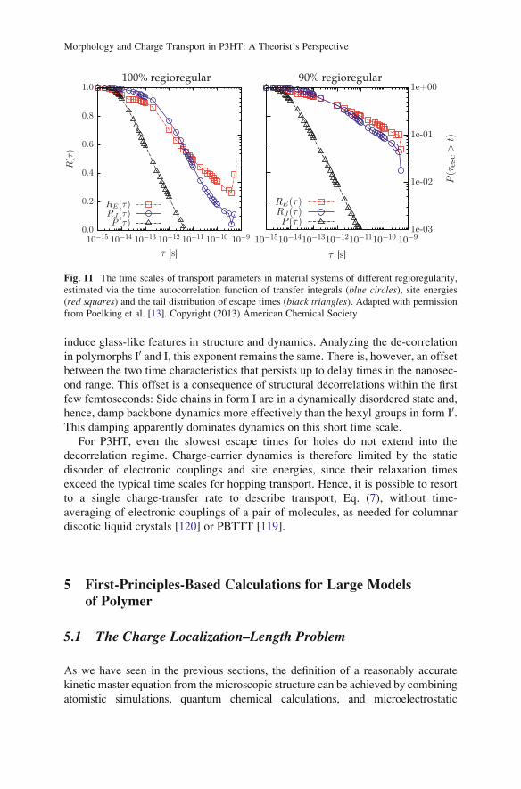
induce glass-like features in structure and dynamics. Analyzing the de-correlation

in polymorphs I0 and I, this exponent remains the same. There is, however, an offset

between the two time characteristics that persists up to delay times in the nanosec-

ond range. This offset is a consequence of structural decorrelations within the first

few femtoseconds: Side chains in form I are in a dynamically disordered state and,

hence, damp backbone dynamics more effectively than the hexyl groups in form I0.This damping apparently dominates dynamics on this short time scale.

For P3HT, even the slowest escape times for holes do not extend into the

decorrelation regime. Charge-carrier dynamics is therefore limited by the static

disorder of electronic couplings and site energies, since their relaxation times

exceed the typical time scales for hopping transport. Hence, it is possible to resort

to a single charge-transfer rate to describe transport, Eq. (7), without time-

averaging of electronic couplings of a pair of molecules, as needed for columnar

discotic liquid crystals [120] or PBTTT [119].

5 First-Principles-Based Calculations for Large Models

of Polymer

5.1 The Charge Localization–Length Problem

As we have seen in the previous sections, the definition of a reasonably accurate

kinetic master equation from the microscopic structure can be achieved by combining

atomistic simulations, quantum chemical calculations, and microelectrostatic

Fig. 11 The time scales of transport parameters in material systems of different regioregularity,

estimated via the time autocorrelation function of transfer integrals (blue circles), site energies

(red squares) and the tail distribution of escape times (black triangles). Adapted with permission

from Poelking et al. [13]. Copyright (2013) American Chemical Society


corrections. These methodologies require the definition of a ‘unit of transport’, i.e., a

region of the polymer where the charge is assumed to reside. For transport in small

molecules, liquid crystals, and some relatively short polymers it is straightforward to

consider the full molecular unit as the unit of transport. It is also reasonable to

consider long oligomers when studying transport in the direction perpendicular to

the π–π stacking in semicrystalline phases. For amorphous regions in fully amor-

phous polymers, or if one is interested in the transport along the π-conjugatedbackbone, further approximations are needed. In the case of amorphous polymers

like poly(p-phenylene vinylene) (PPV), the structure determined by classical simu-

lations [121–123] contains regions where there is a strong deviation from planarity

and it was proposed that the polymeric chain can be divided into conjugated portions

defined as the regions between these conjugation-breaking distortions [124]. This

idea has been used to interpret spectroscopic data but it is very difficult to apply it to

computational systems. First of all, it is not clear how one can rigorously define a

sharp threshold separating the complete conjugation breaking from the full conjuga-

tion between monomers. Moreover, there are many interesting polymers (including

P3HT) that form crystalline domains so extended that no conjugation breaks are

found for hundreds of nanometers [125]. The charge is certainly more localized than

that, either by the disorder present in the semicrystalline phase or by electron–phonon

coupling (evidence of charge localization can be found for example from charge-

modulated spectroscopy [126, 127]). Determination of the localization characteristic

of charge carriers in polymers is another important area of computational investiga-

tion that has been pursued by several groups over the past few years.

To determine the charge localization in a large system there is no other alterna-

tive than computing the electronic wavefunction of a large model system. The

model systems are generated by classical simulation of polymers containing thou-

sands of atoms, so it is not practical to study them in a charged state using quantum-

mechanical methods. A calculation of the electronic structure of such a large model

with an electron less than the neutral state would only yield the ground state,

whereas one is generally interested in the energy distribution and localization of

many charged states. The excited state of the charged simulation box cannot be

computed with modern computational methods and therefore one cannot even

evaluate the nuclear relaxation (reorganization energy) for the hopping between

two states by starting with a large model system. For these reasons, all attempts to

evaluate the wavefunction of a large model of polymers have focused on neutral

systems and have interpreted the one-electron states (the orbitals) as the possible

sites where the excess charge can be localized [107, 108]. Results are normally

presented in terms of a density of states (DOS) and localization length but it should

be noted that these two quantities are computed for systems with orbitals fully filled

and empty above and below the band gap, respectively. Therefore, they cannot be

directly compared with the models in Sect. 4, which include electron and nuclear

polarization but have to make assumptions regarding the localization length.

For the one-electron states to be representative of the actual localization of the

charge carrier, a further condition needs to be satisfied. The charge needs to be

localized predominantly by the conformational disorder of the polymer and not by

C. Poelking et al.

the electron–phonon coupling. If this coupling is particularly strong, the frontier

orbitals may be delocalized over many monomers. However, when an excess

charge is added, the nuclear polarization localizes the charge, completely modify-

ing the electronic wavefunction with respect to the neutral calculation. There is

some general consensus [128, 129] that the localization of the wavefunction in

P3HT largely originates from disorder and not from electron–phonon coupling

because there is a correlation between increased order of P3HT and increased

mobility [20]. Alternatively, one can be convinced that the conformational disorder

is stronger than the electron–phonon coupling by comparing the polaron size of a

perfectly ordered polymer chain with the localization of the orbitals computed from

calculation of large realistic models of disordered chains. If the polaron size of the

perfectly ordered system is much larger than the orbital in the disordered model, it

is acceptable to determine the charge localization from calculations that neglect the

electron–phonon coupling as a first approximation. Calculations for P3HT support

this approximation [108, 130] but it should be noticed that polaron sizes are

strongly dependent on the DFT methodology [131] and that the same assumption

may not hold for the new families of semiconducting polymers [132], where large

conjugated units are more weakly coupled by smaller conjugated linkers.

5.2 Strategies for Large-Scale Electronic-StructureCalculations of Polymer Models

Under the conditions that the calculation of a ground state wavefunction of a

polymer model yields information about the charge localization for the carrier

states, it is still not trivial to carry out such calculations. It is not obvious to know

in advance how large a model of bulk polymer should be in order to reproduce the

DOS and localization length without the results being affected by finite-size effects.

The experience of available calculations with P3HT and PPV suggests that a model

containing several chains of 20–40 monomers displays electronic properties that do

not depend appreciably on the chain length [133] (it should not be forgotten that the

morphology depends on the chain length up to much larger molecular weights

[134]). Such models contain tens of thousands of atoms, a number that is still one

order of magnitude larger than that normally achievable by current software

specialized in linear scaling ab initio calculations, like SIESTA [135] or ONETEP

[136]. It is certainly possible that such methods can be employed in the near future

in benchmark calculations, but it is important to remember that what is needed is a

methodology able to evaluate the wavefunction for many replicas of the equili-

brated systems in order to provide statistically meaningful results.

However, ideas from linear scaling methodologies can be used to develop ad hoc

methods that are able to compute in a more approximate fashion the wavefunction

for large systems. Essentially, all linear scaling methods are based on the definition

of a very localized basis set that reduces the number of matrix elements to be


evaluated to a value that scales linearly with the size of the system [135–137]. For

organic polymers, it seems natural to describe the polymer orbitals as a linear

combination of monomer orbitals. It is possible to reduce the number of orbitals

per monomer to be considered (e.g., from HOMO-1 to LUMO+1 in P3HT), thus

reducing the size of the one-electron effective Hamiltonian. Different schemes have

been proposed for evaluating the diagonal and off-diagonal elements of such a

reduced Hamiltonian, including a fragment molecular orbital approach [138] and a

charge patching method [107, 139, 140]. Their calculation of the matrix elements

shares many points with the methodology described in Sect. 4.3, except that the

calculations are always performed for the neutral state. A general formalism for

such methods has been developed by the quantum chemistry community [137, 141–

143] and has the obvious advantage of being very intuitive: All matrix elements

entering in the Hamiltonian have a clear physical meaning.

The various partitioning schemes proposed for polymer systems are very often

complemented by further approximations that take into account the chemical

structure of the investigated system. As the frontier orbitals are invariably local-

ized on the conjugated fragment of the monomer, while a large fraction of the

molecular weight is taken up by the polymer side chains that do not contribute to

the charge transport states, it is customary to remove the side chains from the

calculation, sometimes substituting them with effective point charges that simu-

late the missing electrostatic effects [133]. For lamellar systems such as P3HT and

PBTTT, it is an excellent approximation to neglect completely the electronic

coupling between lamellae, therefore describing a system that is essentially

two-dimensional [108, 144].

A relatively simple approach that can be considered the simplest possible

Hamiltonian partitioning technique has been proposed recently for the calculation

of the electronic properties of MEH-PPV [133]. Here the amorphous-polymer

model is simply partitioned into subsystems containing single chains (surrounded

by point charges reproducing the local electrostatic potential and with shortened

side chains). The full wavefunction of each single chain can be computed with

routine DFT calculations and the electronic couplings between chains can be

evaluated similarly. The coupling between polymer orbitals localized on different

chains is very small because only a few atoms localized on different chains are in

contact while the orbitals are typically localized over several monomers. A further

reduction in computational cost can be achieved using a small basis set, which, at

least for this type of polymer, does not seem to affect the shape of the DOS or the

localization length.

An alternative approach to full or ad hoc linear scaling DFT methods is calcu-

lation through approximate DFT methods such as the tight binding DFT (DFTB)

[145]. This family of methods has been developed over the past few years and the

most convenient version of the methodology is the self-consistent charge-density

functional tight binding (SCC-DFTB) [146], as implemented for example in the

software DFTB+. An acceleration of one to two orders of magnitudes for the

electronic structure calculation is achieved by an approximate evaluation of the

Kohn–Sham–Fock matrix elements in the atomic-orbital basis. A very broad range

C. Poelking et al.

of applications apart from organic semiconductors have been proposed [143], but

relatively few results have been reported for semiconducting polymers [147] even

though great success has been achieved in the study of charge transfer processes in

biophysical systems [148, 149], which provide a similar level of computational

challenge.

Finally, an obvious choice for calculation of the large-scale electronic structure

would be via semi-empirical methods. These have been the methods of choice for

many years for exploring charge [150] and exciton [151] dynamics in single-chain

polymers containing only carbon and hydrogen (e.g., PPV, polyethylene). How-

ever, there are very few systematic studies of their reliability for polymers

containing heteroatoms such as S, F, Se, and Ge, which are featured in a large

number of new polymers.

Although there seems to be no lack of options for the calculation of the

wavefunction of large models of polymeric systems, these calculations have been

attempted on a very limited number of systems. One of the main objectives of future

computational studies is to perform calibration of these methodologies, whereby

the results obtained with different approximate electronic structure methods on the

same structural models are compared.

5.3 Results from the Computation of the Wavefunctionfor Large-Scale Polymer Models

The calculations performed on models of polymers, according to any of the

methodologies described in the previous section, provide in the first instance the

DOS and a measure of the localization length of the states relevant for transport,

i.e., those located at the edge of the valence (or conduction) band for holes

(or electrons). For all polymers considered (amorphous and semicrystalline), the

states deep in the tail of the DOS are more localized and the localization length

increases as states deeper in the band are considered (see Fig. 12), as predicted by

simplified generic polymer models [152]. The chemical description of these states

in the tail is potentially very useful because it may suggest possible routes for

increasing the charge mobility by reducing the number of trap states.

Calculations suggest that hole trap states (high-energy occupied orbitals) are

found in regions of P3HT where the conjugated backbone is more planar than on

average [108, 153]. The possibility of different degrees of planarity generates

regions where the HOMO–LUMO gap is smaller, coinciding with the more planar

segments of P3HT. Not surprisingly, when regioregularity defects are introduced,

the trap states become localized far away from the regioregularity defect and, for

this reason, the total number of trap states is not much affected by the

regioregularity. This has also been found experimentally [108].

By adopting fast methods for calculation of the electronic structure, it is possible

to monitor the lifetime of these trap states by repeating the electronic structure


calculation for different snapshots obtained via classical molecular dynamics (see

Fig. 13). For P3HT, the most stable trap states are stable for many tens of

picoseconds, i.e., it is possible to think that these trap states are static defects

from the point of view of the moving charge carrier [153]. Further analysis shows

that these local deformations within the semicrystalline domain are stabilized by

gauche conformations in the side chain. A similar analysis on PBTTT shows

instead that the trap states appear and disappear in different parts of the chain

within a few tens of picoseconds, i.e., there are no long-lived trap states in PBTTT

Fig. 12 Left: Average localization length in an ordered region of P3HT with regioregularities of

56% (magenta, lowest curve), 77% (blue), 92% (green) and 100% (red, uppermost curve). Theerror bars of a few selected points are larger in the tail region, indicating the coexistence of

localized and delocalized states in that region. Right: Localization of the orbital density for the

state at the band edge (dark blue regions correspond to higher density) on each P3HT monomer

(represented as a sphere) for different polymer regioregularities. Adapted with permission from

McMahon et al. [108]. Copyright (2013) American Chemical Society

Fig. 13 Localization of the HOMO orbital density on each monomer in a P3HT lamella with low

regioregularity during part of the molecular dynamics trajectory. The orbital density (dark regionscorrespond to higher density) is localized (except at 50 ps) in one of the two regions indicated by

rectangles. Adapted with permission from McMahon et al. [108]. Copyright (2013) American

Chemical Society

C. Poelking et al.

[147]. Considering that it was not possible to find a clear correlation between the

geometry of the chain and the existence of trap states, it was argued that the

excellent charge mobility in PBTTT could be due to the limited number of trap

states that are supported by the PBTTT morphology.

The attempt to correlate the local structure of the polymer with the localization

of the orbitals also yielded some interesting and counterintuitive results [133]. In

amorphous PPV, a significant number of high-energy occupied orbitals was found

in highly bent regions of the polymer spanning two fragments that, by considering

the shape of the polymer, ought to be considered belonging to two separate

conjugated units. Considering all the available studies together, it seems that simple

intuitive arguments are not sufficient to qualitatively predict the relation between

the local geometric structure of a polymer and the localization of its orbitals.

Once the one-electron states of a large system have been evaluated, it is very

challenging to derive a fully satisfactory master equation like Eq. (36) that

describes the hopping rate between these approximate states. Vukmirovic and

Wang have proposed a perturbative expression assuming that these states are

coupled by nonadiabatic coupling terms that can be evaluated explicitly [107] or

can be approximated using the overlap between the absolute value of the

wavefunction [154]. Remarkably, the proposed expression does not contain the

effect of nuclear polarization in the presence of an additional charge (reorganization

energy) and so it is strictly valid in the limit of vanishing reorganization energy like

Miller–Abrahams rates [155]. Using this approach it was highlighted that the DOS

does not contain all the information needed to evaluate the mobility and that it is

possible to have reduced broadening of the DOS due to increased order, but still

have lowmobility because the coupling between states is reduced [156]. Alternative

methods for combining nuclear polarization and disorder effects have been pro-

posed but they have so far only been applied to highly simplified model systems

[157, 158].

Ideally, such large-scale calculations should be able to incorporate the effect of

nuclear and electronic polarization but, as outlined in Sect. 5.2, it is not clear how

such generalizations could be introduced within the available methodologies.

6 Outlook

To conclude, substantial method development is still required in order to achieve

parameter-free modeling of organic semiconductors. Imperative for predicting

large-scale morphologies are accurate polarizable force fields and computationally

efficient coarse-grained models. These models should be capable of describing

backbone crystallization and allow for reintroduction of atomistic details. Essential

for charge transport are extensions of large-scale, first-principles methods to

charged states. Challenges are the incorporation of polaronic effects and a unified

description of charge transfer along a single chain and between conjugated seg-

ments located on different chains. Last but not least, molecular charge transfer


parameters must be included into a hybrid kinetic Monte–Carlo scheme, with

transfer rates updated on the fly to account for long-range electrostatic and polar-

ization effects.

Acknowledgments This work was partly supported by the DFG program IRTG 1404, DFG grant

SPP 1355, and BMBF grants MEDOS (FKZ 03EK3503B), MESOMERIE (FKZ 13N10723), and

MORPHEUS (FKZ 13N11704). We thank Patrick Gemunden for fruitful collaborations and

discussions. We are grateful to Jeroen van der Holst, Mara Jochum and Kurt Kremer for critical

reading of the manuscript.

References

1. McCullough RD (1998) Adv Mater 10(2):93–116

2. McCullough RD, Lowe RD (1992) Chem Commun 1992(1):70

3. Meyer V (1883) Berichte der deutschen chemischen Gesellschaft 16(1):1465

4. Yamamoto T, Sanechika K, Yamamoto A (1980) J Polym Sci Polym Lett Ed 18(1):9

5. Lin JWP, Dudek LP (1980) J Polym Sci Polym Chem Ed 18(9):2869

6. Elsenbaumer R, Jen K, Oboodi R (1986) Synth Met 15(2–3):169

7. Perepichka IF, Perepichka DF, Meng H (2009) Thiophene-based materials for electrolumi-

nescent applications. In: Perepichka IF, Perepichka DF (ed), Handbook of thiophene-based

materials. Wiley, Hoboken, p 695–756

8. Prosa TJ, Winokur MJ, McCullough RD (1996) Macromolecules 29(10):3654

9. Brinkmann M (2011) J Polym Sci B Polym Phys 49(17):1218

10. Wu Z, Petzold A, Henze T, Thurn-Albrecht T, Lohwasser RH, Sommer M, Thelakkat M

(2010) Macromolecules 43(10):4646

11. Yuan Y, Zhang J, Sun J, Hu J, Zhang T, Duan Y (2011) Macromolecules 44(23):9341

12. Dudenko D, Kiersnowski A, Shu J, Pisula W, Sebastiani D, Spiess HW, Hansen MR (2012)

Angew Chem Int Ed 51(44):11068

13. Poelking C, Andrienko D (2013) Macromolecules 46(22):8941

14. Shimomura T, Takahashi T, Ichimura Y, Nakagawa S, Noguchi K, Heike S, Hashizume T

(2011) Phys Rev B 83(11):115314

15. Li G, Shrotriya V, Huang J, Yao Y, Moriarty T, Emery K, Yang Y (2005) Nat Mater 4

(11):864

16. Mauer R, Kastler M, Laquai F (2010) Adv Funct Mater 20(13):2085

17. Ballantyne AM, Chen L, Dane J, Hammant T, Braun FM, Heeney M, Duffy W, McCulloch I,

Bradley DDC, Nelson J (2008) Adv Funct Mater 18(16):2373–2380

18. Tsumura A, Koezuka H, Ando T (1986) Appl Phys Lett 49(18):1210

19. Bao Z, Dodabalapur A, Lovinger AJ (1996) Appl Phys Lett 69(26):4108

20. Chang JF, Clark J, Zhao N, Sirringhaus H, Breiby DW, An-dreasen JW, Nielsen MM,

Giles M, Heeney M, McCulloch I (2006) Phys Rev B 74(11):115318

21. Kline RJ, McGehee MD, Kadnikova EN, Liu J, Frechet JMJ, Toney MF (2005) Macromol-

ecules 38(8):3312

22. Zen A, Paum J, Hirschmann S, ZhuangW, Jaiser F, Asawapirom U, Rabe JP, Scherf U, Neher

D (2004) Adv Funct Mater 14(8):757–764

23. Merlo JA, Frisbie CD (2003) J Polym Sci B Polym Phys 41(21):2674–2680

24. Bolsee JC, Oosterbaan WD, Lutsen L, Vanderzande D, Manca J (2011) Org Electron 12

(12):2084

25. Raos G, Famulari A, Marcon V (2003) Chem Phys Lett 379(3–4):364

26. Darling SB, Sternberg M (2009) J Phys Chem B 113(18):6215, PMID: 19290596

27. Marchiori C, Koehler M (2010) Synth Met 160(7–8):643

C. Poelking et al.

28. Bhatta RS, Yimer YY, Tsige M, Perry DS (2012) Comput Theor Chem 995:36

29. Tsuzuki S, Honda K, Azumi R (2002) J Am Chem Soc 124(41):12200

30. Bhatta RS, Perry DS (2013) Comput Theor Chem 1008:90

31. Baggioli A, Famulari A (2014) Phys Chem Chem Phys 16:3983-3994

32. Maillard A, Rochefort A (2009) Phys Rev B 79(11):115207

33. Colle R, Grosso G, Ronzani A, Zicovich-Wilson CM (2011) Physica Status Solidi B 248

(6):1360–1368

34. Xie W, Sun YY, Zhang SB, Northrup JE (2011) Phys Rev B 83(18):184117

35. Famulari A, Raos G, Baggioli A, Casalegno M, Po R, Meille SV (2012) J Phys Chem B 116

(49):14504

36. Dag S, Wang LW (2010) J Phys Chem B 114(18):5997

37. Marcon V, Raos G (2004) J Phys Chem B 108(46):18053

38. Moreno M, Casalegno M, Raos G, Meille SV, Po R (2010) J Phys Chem B 114(4):1591

39. To TT, Adams S (2012) Nanosci Nanotechnol Lett 4(7):703

40. Bhatta RS, Yimer YY, Perry DS, Tsige M (2013) J Phys Chem B 117(34):10035

41. Melis C, Colombo L, Mattoni A (2011) J Phys Chem C 115(2):576

42. Alexiadis O, Mavrantzas VG (2013) Macromolecules 46(6):2450

43. Curco D, Aleman C (2007) J Comput Chem 28(10):1743–1749

44. Zhang G, Pei Y, Ma J, Yin K, Chen CL (2004) J Phys Chem B 108(22):6988

45. Huang DM, Faller R, Do K, Moule AJ (2010) J Chem Theory Comput 6(2):526

46. Do K, Huang DM, Faller R, Moule AJ (2010) Phys Chem Chem Phys 12(44):14735

47. Yimer YY, Dhinojwala A, Tsige M (2012) J Chem Phys 137(4):044703

48. Reddy S, Kuppa VK (2012) Synth Met 162(23):2117

49. D’Avino G, Mothy S, Muccioli L, Zannoni C, Wang L, Cornil J, Beljonne D, Castet F (2013)

J Phys Chem C 117(25):12981

50. Lee CK, Pao CW, Chu CW (2011) Energ Environ Sci 4(10):4124

51. Muller M (2011) J Stat Phys 145(4):967

52. Noid WG (2013) J Chem Phys 139(9):090901

53. Kremer K, Muller-Plathe F (2002) Mol Simulat 28(8–9):729

54. Lyubartsev AP, Laaksonen A (1995) Phys Rev E 52(4):3730

55. Izvekov S, Voth GA (2005) J Phys Chem B 109(7):2469

56. Noid WG, Chu J, Ayton GS, Krishna V, Izvekov S, Voth GA, Das A, Andersen HC (2008) J

Chem Phys 128:244114

57. Shell MS (2008) J Chem Phys 129(14):144108

58. Daoulas KC, Muller M (2010) Comparison of simulations of lipid membranes with mem-

branes of block copolymers. In: Meier WP, Knoll W (eds) Polymer membranes/

biomembranes. Advances in Polymer Science, vol 224. Springer, Berlin Heidelberg, pp

43–85

59. Jankowski E, Marsh HS, Jayaraman A (2013) Macromolecules 46(14):5775

60. Schwarz KN, Kee TW, Huang DM (2013) Nanoscale 5(5):2017

61. Reith D, Putz M, Muller-Plathe F (2003) J Comput Chem 24(13):1624–1636

62. Carbone P, Varzaneh HAK, Chen X, Muller-Plathe F (2008) J Chem Phys 128(6):064904

63. Daoulas KC, Ruhle V, Kremer K (2012) J Phys Condens Mat 24(28):284121

64. Gemunden P, Poelking C, Kremer K, Andrienko D, Daoulas KC (2013) Macromolecules 46

(14):5762

65. Stingelin N (2012) Polym Int 61(6):866–873

66. Ho V, Boudouris BW, Segalman RA (2010) Macromolecules 43(19):7895

67. Holyst R, Vilgis TA (1996) Macromol Theor Simulat 5(4):573–643

68. HammM, Goldbeck-Wood G, Zvelindovsky AV, Sevink GJA, Fraaije JGEM (2002) J Chem

Phys 116(7):3152

69. Wang Q (2011) Soft Matter 7(8):3711

70. Pryamitsyn V, Ganesan V (2004) J Chem Phys 120(12):5824

71. Kumar NA, Ganesan V (2012) J Chem Phys 136(10):101101


72. Vettorel T, Besold G, Kremer K (2010) Soft Matter 6(10):2282

73. Helfand E, Tagami Y (2003) J Chem Phys 56(7):3592

74. Daoulas KC, Muller M (2006) J Chem Phys 125(18):184904

75. Detcheverry FA, Pike DQ, Nealey PF, Muller M, Pablo JJD (2009) Faraday Discuss 144:111

76. Kron AK (1965) Polym Sci USSR 7(7):1361

77. Wall FT, Mandel F (2008) J Chem Phys 63(11):4592

78. Ruhle V, Kirkpatrick J, Andrienko D (2010) J Chem Phys 132(13):134103

79. Marcus RA (1993) Rev Mod Phys 65(3):599

80. May V, Kuhn O (2011) Charge and energy transfer dynamics in molecular systems, 3rd edn.

Wiley-VCH, Weinheim

81. Grabert H, Weiss U (1985) Phys Rev Lett 54(15):1605

82. Fisher MPA, Dorsey AT (1985) Phys Rev Lett 54(15):1609

83. Ruhle V, Lukyanov A, May F, Schrader M, Vehoff T, Kirkpatrick J, Baumeier B, Andrienko

D (2011) J Chem Theory Comput 7(10):3335

84. Asadi K, Kronemeijer AJ, Cramer T, Jan Anton Koster L, Blom PWM, de Leeuw DM (2013)

Nat Commun 4:1710

85. Reimers JR (2001) J Chem Phys 115(20):9103

86. Hsu CP (2009) Accounts Chem Res 42(4):509

87. Valeev EF, Coropceanu V, da Silva Filho DA, Salman S, Bredas JL (2006) J Am Chem Soc

128(30):9882

88. Bredas JL, Calbert JP, Filho DADS, Cornil J (2002) Proc Natl Acad Sci USA 99(9):5804

89. Coropceanu V, Cornil J, da Silva Filho DA, Olivier Y, Silbey R, Bredas JL (2007) Chem Rev

107(4):926

90. Kirkpatrick J (2008) Int J Quantum Chem 108(1):51, Bibtex: Kirkpatrick 2008

91. Baumeier B, Kirkpatrick J, Andrienko D (2010) Phys Chem Chem Phys 12(36):11103

92. Fogel Y, Zhi L, Rouhanipour A, Andrienko D, Rader HJ, Mullen K (2009) Macromolecules

42(18):6878

93. Scher H, Alexander S, Montroll EW (1980) Proc Natl Acad Sci U S A 77(7):3758

94. Stone AJ (1997) The theory of intermolecular forces. Clarendon, Oxford

95. Hattig C (1996) Chem Phys Lett 260(3–4):341

96. Hattig C, Heß BA (1994) Mol Phys 81(4):813

97. Verstraelen T, Pauwels E, De Proft F, Van Speybroeck V, Geer-lings P, Waroquier M (2012)

J ChemTheory Comput 8(2):661

98. Breneman CM, Wiberg KB (1990) J Comput Chem 11(3):361–373

99. Stone A, Alderton M (1985) Mol Phys 56(5):1047

100. Stone AJ (2005) J Chem Theory Comput 1(6):1128

101. Kramer C, Bereau T, Spinn A, Liedl KR, Gedeck P, Meuwly M (2013) J Chem Inf Model 53

(12):3410

102. Chirlian LE, Francl MM (1987) J Comput Chem 8(6):894

103. Thole B (1981) Chem Phys 59(3):341

104. van Duijnen PT, Swart M (1998) J Phys Chem A 102(14):2399

105. Applequist J, Carl JR, Fung KK (1972) J Am Chem Soc 94(9):2952

106. Ren P, Ponder JW (2003) J Phys Chem B 107(24):5933

107. Vukmirovic N, Wang LW (2011) J Phys Chem B 115(8):1792

108. McMahon DP, Cheung DL, Goris L, Dacuna J, Salleo A, Troisi A (2011) J Phys Chem C 115

(39):19386

109. Baessler H (1993) Phys Status Solidi B 175(1):15

110. Lan YK, Yang CH, Yang HC (2010) Polym Int 59(1):16

111. Kirkpatrick J, Marcon V, Nelson J, Kremer K, Andrienko D (2007) Phys Rev Lett 98

(22):227402

112. Marcon V, Kirkpatrick J, Pisula W, Andrienko D (2008) Phys Status Solidi B 245(5):

820–824

C. Poelking et al.

113. Andrienko D, Kirkpatrick J, Marcon V, Nelson J, Kremer K (2008) Phys Status Solidi B 245

(5):830

114. Nelson J, Kwiatkowski JJ, Kirkpatrick J, Frost JM (2009) Accounts Chem Res 42(11):1768

115. May F, Marcon V, Hansen MR, Grozema F, Andrienko D (2011) J Mater Chem 21(26):9538

116. Schrader M, Fitzner R, Hein M, Elschner C, Baumeier B, Leo K, Riede M, Bauerle P,

Andrienko D (2012) J Am Chem Soc 134(13):6052

117. Schrader M, Korner C, Elschner C, Andrienko D (2012) J Mater Chem 22(41):22258

118. Mas-Torrent M, Boer DD, Durkut M, Hadley P, Schenning APHJ (2004) Nanotechnology 15

(4):S265

119. Poelking C, Ivanov V, Kremer K, Risko C, Bredas JL, Andrienko D, Eunkyung C (2013) J

Phys Chem C 117(4):1633

120. Olivier Y, Muccioli L, Lemaur V, Geerts YH, Zannoni C, Cornil J (2009) J Phys Chem B 113

(43):14102

121. De Leener C, Hennebicq E, Sancho-Garcia JC, Beljonne D (2009) J Phys Chem B 113

(5):1311

122. DuBay KH, Hall ML, Hughes TF, Wu C, Reichman DR, Friesner RA (2012) J Chem Theory

Comput 8(11):4556

123. Kumar P, Mehta A, Mahurin SM, Dai S, Dadmun MD, Sumpter BG, Barnes MD (2004)

Macromolecules 37(16):6132

124. Collini E, Scholes GD (2009) Science 323(5912):369, PMID: 19150843

125. Salleo A, Kline RJ, DeLongchamp DM, Chabinyc ML (2010) Adv Mater 22(34):3812–3838

126. Beljonne D, Cornil J, Sirringhaus H, Brown PJ, Shkunov M, Friend RH, Bredas JL (2001)

Adv Funct Mater 11(3):229–234

127. Brown PJ, Sirringhaus H, Harrison M, Shkunov M, Friend RH (2001) Phys Rev B 63

(12):125204

128. Magin EH, Borsenberger PM (1993) J Appl Phys 73(2):787

129. Van der Auweraer M, De Schryver FC, Borsenberger PM, Bassler H (1994) Adv Mater 6

(3):199–213

130. Zade SS, Zamoshchik N, Bendikov M (2011) Accounts Chem Res 44(1):14

131. Nayyar IH, Batista ER, Tretiak S, Saxena A, Smith DL, Martin RL (2013) J Chem Theory

Comput 9(2):1144

132. Bronstein H, Chen Z, Ashraf RS, Zhang W, Du J, Durrant JR, Shakya Tuladhar P, Song K,

Watkins SE, Geerts Y, Wienk MM, Janssen RAJ, Anthopoulos T, Sirringhaus H, Heeney M,

McCul-loch I (2011) J Am Chem Soc 133(10):3272

133. Qin T, Troisi A (2013) J Am Chem Soc 135(30):11247

134. Shaked S, Tal S, Roichman Y, Razin A, Xiao S, Eichen Y, Tessler N (2003) Adv Mater 15

(11):913–916

135. Soler JM, Artacho E, Gale JD, Garcıa A, Junquera J, Ordejon P, Sanchez-Portal D (2002) J

Phys Condens Mat 14(11):2745

136. Skylaris CK, Haynes PD, Mostofi AA, Payne MC (2005) J Chem Phys 122(8):084119

137. Gordon MS, Mullin JM, Pruitt SR, Roskop LB, Slipchenko LV, Boatz JA (2009) J Phys

Chem B 113(29):9646

138. McMahon DP, Troisi A (2009) Chem Phys Lett 480(4–6):210

139. Vukmirovic N, Wang LW (2009) J Phys Chem B 113(2):409

140. Vukmirovic N, Wang LW (2009) Nano Lett 9(12):3996

141. Fedorov DG, Kitaura K (2007) J Phys Chem A 111(30):6904

142. Kitaura K, Ikeo E, Asada T, Nakano T, Uebayasi M (1999) Chem PhysLett 313(3–4):701

143. Kubar T, Elstner M (2013) J R Soc Interface 10(87):20130415, PMID: 23883952

144. Liu J, Sun Y, Gao X, Xing R, Zheng L, Wu S, Geng Y, Han Y (2011) Langmuir 27(7):4212

145. Porezag D, Frauenheim T, Kohler T, Seifert G, Kaschner R (1995) Phys Rev B 51(19):12947

146. Elstner M, Porezag D, Jungnickel G, Elsner J, Haugk M, Frauen-heim T, Suhai S, Seifert G

(1998) Phys Rev B 58(11):7260

147. Liu T, Troisi A (2014) Adv Funct Mater 24(7):925-933


148. Kubar T, Elstner M (2010) J Phys Chem B 114(34):11221

149. Kubar T, Kleinekathofer U, Elstner M (2009) J Phys Chem B 113(39):13107

150. Johansson A´, Stafstrom S (2001) Phys Rev Lett 86(16):3602

151. Barford W, Trembath D (2009) Phys Rev B 80(16):165418

152. Noriega R, Rivnay J, Vandewal K, Koch FPV, Stingelin N, Smith P, Toney MF, Salleo A

(2013) Nat Mater 12(11):1038

153. Cheung DL, McMahon DP, Troisi A (2009) J Am Chem Soc 131(31):11179

154. Vukmirovic N, Wang LW (2010) Appl Phys Lett 97(4):043305

155. Miller A, Abrahams E (1960) Phys Rev 120(3):745

156. Vukmirovic N (2013) Phys Chem Chem Phys 15(10):3543

157. Bronold FX, Alvermann A, Fehske H (2004) Phil Mag 84(7):673

158. Fornari RP, Troisi A (2014) Phys Chem Chem Phys 16(21):9997

C. Poelking et al.

Morphology and Charge Transport in P3HT: A Theorist’s …andrienk/publications/poelk… · ·...

Documents

Transcript of Morphology and Charge Transport in P3HT: A Theorist’s …andrienk/publications/poelk… · ·...