[Proc. SPIE Vol. 1769 \Image Algrebra and Morphological Image Processing III", pp. 212{226, San Diego CA, July1992]

Morphological Image Processing and Network Analysisof Cornea Endothelial Cell Images

Luc VincentXerox Imaging Systems

9 Centennial Drive, Peabody, MA 01960

Barry MastersDepartment of Anatomy and Cell Biology

Uniformed Services University of the Health Sciences, Bethesda, MD 20814{4799

Abstract

In this paper, we propose a robust and accurate method for segmenting grayscale images of corneal endothelialtissue. Its �rst step consists in the extraction of markers of the corneal cells using a dome extractor based onmorphological grayscale reconstruction. Then, marker-driven watershed segmentation yields binary images of thecorneal cell network. From these images, we derive histograms of the cell sizes and number of neighbors, whichprovide quantitative information about the condition of the cornea. We also construct the neighborhood graph ofthe corneal cells, whose granulometric analysis yields information on the distribution of cells with large number ofneighbors in the tissue. Lastly, these results help us propose a model for the corneal cell death phenomenon. Thenumerical simulation of this model exhibits a very good match with our experimental results. This model not onlyallows us to re�ne our understanding of the phenomenon: combined with our results, it enables the estimation ofthe percentage of cells having died in a given corneal endothelial tissue.

1 Introduction

The human cornea is a 500 microns thick, transparent tissue which covers the anterior surface of the eye. The corneaand the ocular lens are the refracting elements of the eye. At the posterior side of the cornea is situated a single,connected layer of endothelial cells. These cells, polygonal in shape, are about 20 microns across and about fourmicrons thick. At birth, the corneal endothelial cells are all hexagons. Cells die as the cornea ages, but there is nonew cell division when a cell die: instead, the surrounding cells elongate to �ll in the gap and therefore, the averagesize of the endothelial cells increases throughout life. The corneal endothelial cells are responsible for the maintenanceof corneal transparency; active transport enzyme systems pump ions into the regions between the cells, the resultingosmotic force drives uid out of the cornea into the aqueous humour. In the normal eye, the uid transport isin balance with the uid transport leakage from the aqueous humour into the cornea and corneal transparency ismaintained. In diseased or injured corneas, this balance is disturbed and the cornea swells and loses its transparency.The analysis of corneal endothelial cell size and shape is extremely important for diagnostic purposes.

In this paper, we propose a new and robust method to segment grayscale images of corneal endothelial celltissue. This method is based on advanced morphological transformations [18, 19], including grayscale reconstruction[25] and watersheds [2, 27]. It allows us to precisely and robustly extract the cell outlines, which is the �rst steptowards the automatic analysis of corneal tissues. This method is described in the section 4.

In section 5, we �rst derive shape and size measurements from the obtained binary images. Histograms ofcell sizes and number of edges turn out to convey a lot of information on the corneal condition. We then buildneighborhood graphs on the corneal tissue and use morphological granuometries of these graphs [13, 21] to study thedistribution of large and small cells within the tissue.

Lastly, in section 6, we model the cell death phenomenon. Numerical simulations of this model exhibit a verygood match with the results found experimentally in section 5. Comparing the measurements on a given cornealtissue with the model allows us to estimate the percentage of cells having died, and therefore provide a good estimateof the condition of the cornea.

2 Previous work

Several previous studies have reported attempts to use computer assisted image analysis in order to extract cell sizeand shape from photomicrographs of the human cornea endothelium. The main problem has been the location ofthe cell boundaries in the gray level image obtained from a photograph or a digitized video frame.

The initial work on the problem of edge detection is represented by the works of Laing et al. [10] and Fabian etal. [4]: photographs or video images were digitized and histogram manipulation followed by thresholding was used foredge detection of the cell boudaries. More elegant image processing techniques were recently proposed by Cazuguelet al. [3]: histogram equalization, top-hat �lter followed by skeleton by in uence zones [11], and Yu et al.: adaptivelocal enhancement, low pass �lter and matched �lters with kernels corresponding to di�erent orientations. . .

Still, none of these solutions seem to be robust enough to deal with a vast variety of initial images (contrast,noise level, lighting conditions may greatly vary from one case to the other). Furthermore, there remains a lot ofwork to be done on the interpretation of the results (i.e., of the binary images obtained after segmentation). To ourknowledge, no published work has ever gone beyond the simple measurement of cell areas and number of neighbors.

3 Data Acquisition

In our study, a corneal wide-�eld specular microscope [9, 17, 14] was used to obtain the gray level images of a �eldof several hundred cells from normal human patients. The principle of the microscope is that a slit of light is imagedon the cornea and the region of the interface between the endothelial cell layer and the aqueous humour exhibits ahigh re ecticity due to the shape change in refractive index. The microscope operated in the specular mode: thespecular re ection of light from the boundary between the endothelial cells and the aqueous humour forms the image.The cell borders have stronger specular re ection than the other regions of the cells and this generates the imagecontrast. The scattered light from this interface is imaged onto a �lm plane in a camera. A ash of light is used toeliminate motion e�ects on the image. The design of the specular microscope eliminated the bright surface re ectionfrom the air-cornea surface, since an applanating microscope objective is used to match the refractive index to thecornea. An example of the images of our test suite is shown in Fig. 1.

4 Segmentation

We illustrate our segmentation technique on a smaller image, shown in Fig. 2(a). Notice the very irregular lighting,which makes it impossible to use any direct thresholding mechanism. On this image and in Fig. 1, one can alsoobserve that the cells can vary quite a bit in size. This remark becomes even more true with damaged or diseasedcornea. Nevertheless, the cells form a contiguous partition of the space: the separation between any two neighboringcell is a thin dark line of relatively constant thickness. Therefore, it seems natural to try to detect these dark celloutlines using the top-hat transformation.

The top-hat transformation is a morphological segmentation tool which was originally described in [15]. In itsvalley-detection version, it consists of subtracting the image I under study from I closed by a given structuring

Figure 1 : Image of a corneal endothelial cell tissue.

element [18]. Here, a top-hat of Fig. 2(a) with respect to a small disc yields Fig. 2(b), where the cell separationsappear clearly.

However, due to the variations in contrast from the center of the image to, e.g., the top right corner, it isimpossible to set a correct threshold for this image: the threshold shown in Fig. 2(c) is appropriate for the centerof the image, but on the top corners, the network of cell boundaries gets disconnected. On the other hand, a lowerthreshold value would correctly extract the cell outlines in the top part of the image, but overconnect the network inthe central area. Furthermore, in each of the images we looked at, the \best" threshold value highly depended on theimage contrast and always had to be manually adjusted. Therefore, although it is at the basis of already publishedwork [3], we did not retain the top-hat transformation in our �nal segmentation algorithm.

(a) (b) (c)

Figure 2 : Image used to illustrate our segmentation method (a), top-hat (b)and threshold of this top-hat (c).

Instead, we chose to �rst preprocess our images using a simple morphological �lter in order to remove the impulsenoise while preserving the valleys (separating lines between cells). An alternated sequential �lter (ASF) of small size

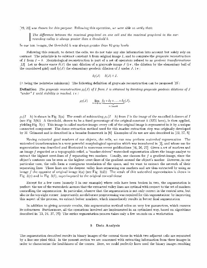
[19, 20] was chosen for this purpose. Following this operation, we were able to verify that:

The di�erence between the maximal gray-level on one cell and the maximal gray-level in the sur-rounding valley is always greater than a threshold h.

In our test images, the threshold h was always greater than 10 gray levels.

Following this remark, to detect the cells, we do not take any size information into account but solely rely oncontrast. The principle is to subtract constant h from original image I , and to compute the grayscale reconstructionof I from I � h. Morphological reconstruction is part of a set of operators refered to as geodesic transformations[12]. Let us denote enote �(J) the unit dilation of a grayscale image J (i.e., the dilation by the elementary ball ofthe considered grid) and �I(J) the elementary geodesic dilation of I under J , i.e.:

�I(J) = �(J) ^ I:

(^ being the pointwise minimum). The following de�nition of grayscale reconstruction can be proposed [25]:

De�nition The grayscale reconstruction �I(J) of I from J is obtained by iterating grayscale geodesic dilations of J\under" I until stability is reached, i.e.:

�I(J) = limn!+1

�I � �I � : : : � �I| {z }n times

(J):

�I(I � h) is shown in Fig. 3(a). The result of subtracting �I(I �h) from I is the image of the so-called h-domes of I(see Fig. 3(b)). A threshold, chosen to be a �xed percentage of the original constant h (33% here), is then applied,yielding Fig. 3(c). This image is called marker-image: every cell of the original image is represented in it by a uniqueconnected component. The dome extraction method used for this marker extraction step was originally developedby M. Grimaud and is described in a broader framework in [6]. Examples of its use are also described in [22, 27, 5].

Having extracted good markers of our objects, the cells, we can now perform watershed segmentation. Thewatershed transformation is a very powerful morphological operation which was introduced in [2], and whose use forsegmentation was described and illustrated in numerous recent publications [16, 26, 27]. Given a set of markers andan image f regarded as a topographic relief, a \marker-driven" watershed segmentation allows the image analyst toextract the highest crest-lines of f separating two markers. Usually, one chooses for f a gradient-image, since theobject's contours can be seen as the highest crest-lines of the gradient around the object's marker. However, in ourparticular case, the cells form a contiguous tesselation of the space, and we want to extract the network of theirseparating lines. These lines are the deepest valley lines separating our markers and are thus extracted by using asimage f the opposite of original image 2(a) (see Fig. 3(d)). The result of this watershed segmentation is shown inFig. 3(e) and in Fig. 3(f), superimposed to the original corneal tissue.

Except for a few cases (namely 5 in our example) where cells have been broken in two, the segmentation isperfect: the use of the watersheds assures that the extracted valley lines are optimal with respect to the set of markerscontrolling the segmentation. In particular, observe that the segmentation is not only correct in the central area, butalso in the top-right corner. Importantly, no elaborate preprocessing was required for this segmentation: by improvingthis aspect of the process, we extract better markers, which immediately results in better �nal segmentation.

In addition to giving accurate results, this segmentation method relies on very few parameters, which ensuresits robustness. Furthermore, all the operations involved are implemented in an optimized way, based on algorithmsdescribed in [23, 24, 27, 25]: The entire segmentation process takes only a few seconds on a workstation.

5 Data Analysis

The segmentation described results in binary images of the corneal tissue in which two adjacent cells are separatedby a line one pixel thick. In the present section we are concerned with extracting information from these images inorder to characterize the healthiness of the cornea. Here, we could perfectly have used the binary images resulting

(a) after reconstruction (b) extracted domes (c) cell markers

(d) inverted original image (e) watershed segmentation (f) result overlayed on original image

Figure 3 : Illustration of the segmentation method

from our prior segmentation step. However, a consistent set of grayscale images of cornea at di�erent ages was notavailable. Therefore, in the present section and the followings, we had to make use of older data, previously collectedthrough the manual tracing of corneal endothelial tissue images. These images were digitized and a simple binaryprocessing allowed us to obtain the binary images shown in Figs. 4(a){(c), corresponding to corneas at increasinglevels of deterioration.

(a) (b)

(c)

Figure 4 : Three di�erent cases of segmented binary images

5.1 Size and shape of the cells

These images exhibit an increasing level of disorder. As mentioned in the introduction, this is due to the fact thatwith aging, corneal cells die and are not replaced by new cells via cell division, as in other bodily tissues. Here, theneighboring cells elongate to �ll in the gap left by the dead cell. Therefore, with aging, many cells tend to becomebigger. This phenomenon can be brought to light by simply assigning to each cell of Figs. 4(a){(c) a gray-level valueequals to its area (number of pixels). The resulting images are shown in Figs. 5(a){(c). The gray-level informationcontained in these images makes the phenomenon of disorder appear even more clearly1. Fig. 6 shows that thehistograms of cell sizes for the three cases (a), (b) and (c) are increasingly distributed.

Classic morphological granulometries can also be used on Figs. 5(a){(c). Recall that, given a convex structuringelement B, whose homothetics are denoted (Bn)n�0:

B0 = f~ogB1 = B

8n � 1; Bn+1 = Bn �B;

the family of openings ( Bn)n�0 constitutes a granulometry, as de�ned by Matheron [13]. The corresponding gran-ulometry function g(I) of a binary image I is then given by [26, 24]:

g(I)

�DI �! ZZ

p 7�! minfk 2 ZZ+ j Bk (p) = 0g:

In other words, g(I) associates with every pixel p of I the largest n such that Bn(I)(p) = 1. The granulometryfunction of image 4(b) with respect to a family of squares is shown in Fig. 7. This image is quite similar to Fig. 5(b),which accounts for the fact that our corneal cells are convex polygons with little elongation. The same remark isvalid for Figs. 4(a) and (c). Therefore, granulometric analysis of our images does not yield much useful additionalquantitative information.

1Note that the 5 lightest-colored cells of image 5(a) correspond to segmentation errors where two cells have been connected into one!

(a) (b)

(c)

Figure 5 : After assigning to each cell of the tissues in Fig. 4 a value (gray-level) equal to its area.

0

5

10

15

20

25

30

35

40

case (c)case (b)case (a)

Figure 6 : Histograms of corneal cell sizes for Figs. 4(a){(c).

Figure 7 : Granulometry function of image 4(b).

The growth of the corneal cells is accompanied by a modi�cation of their number of edges: as cells grow and altertheir shapes to �ll in the gap left by a dead cell, some of these polygonal cells increase their number of edges, whileothers end up with a smaller number of edges. An attempt at modeling this phenomenon is proposed in section 6. Todetermine the number of edges of a corneal cell, it su�ces to extract its number of neighboring cells. To this purpose,we use contour tracking algorithms described in [22] to determine the adjacency graph of the corneal tissue: Thisgraph is a triangulation in which every vertex corresponds to a unique cell. There is also a one to one correspondencebetween the edges of this triangulation and the neighborhood relationships between cells of the initial tissue (seeFig. 8). Using this graph, it is straightforward to assign to each cell its number of neighbors, as is done in Fig. 92.

Figure 8 : Adjacency graph of the cells of image 4(b).

(a) (b)

(c)

Figure 9 : Assigning to the cells of the images in Fig. 4 a gray-level equal totheir number of neighbors.

This �gure illustrates the same trend as Fig. 5, namely an increasing number of disorder, characterized by theincreasing number of cells with 5, 7 or even 8 neighbors from (a) to (c). The histograms of cell number of neighborsfor cases (a), (b) and (c) are shown in Fig. 10. Up to some scaling coe�cients, these histograms are very similar tothose of Fig. 6. This shows the strong|and intuitively clear|correlation existing between size and number of edgesof the corneal cells. Due to their fewer number of possible values (the number of edges basically varies between 3and 8), these histograms of number of neighbors are easier to interpret than the size histograms. Therefore, fromnow on, we shall focus on the number of neighbors of our corneal cells.

5.2 Spatial distribution of the corneal cells

Now that we have characterized the size and shape of our cells, we want to know whether the cell death phenomenonoccurs with equal probability across the whole tissue. In other words, we would like to �nd out if cells tend to die at

2For the sake of display, the cells on the border of the image have been assigned value 4.

0

20

40

60

80

100

proportions of cellswith 3 to 8 sides

4 sides

8 sides

7 sides

5 sides

6 sides

case (a) case (b) case (c)

Figure 10 : Histograms of the number of neighbors for Figs. 4(a){(c).

speci�c locations, like for example around large cells. Since the appeareance of large and|to a lesser extend|smallcells (resp. cells with many and few neighbors) is directly related to cell death, it seems interesting to study theirdistribution in the rest of the corneal tissue.

To this end, we applied morphological tools originally described in in [21] and detailed in [22, 7], namelygranulometries on graphs. Recall that, given a non-oriented graph G = (V;E), with V as set of vertices and E as setof edges, and f a mapping from V to the set of real numbers IR, the elementary graph-dilation of f , denoted �(f),is characterized by:

8v 2 V; �(f)(v) = maxff(v0) j v0 = v or (v; v0) 2 Eg:

In simpler terms, graph-dilating f is equivalent to assigning to each vertex v the maximal value of f on the verticesin the neighborhood of v. Erosions, openings and closings on graphs can be de�ned in the same was [21].

In the present study, the graph structure is given by the triangulation (see Fig. 8) and the mapping f associateswith each vertex the number of neighbors of the corresponding cell. Performing a granulometry by closings of thisgraph allows us to bring to light the clusters of cells with large number of neighbors, as illustrated by Fig. 11. Foreach closing of size k > 0, we compute the granulometry coe�cient Cf (k) as:

Cf (k) =

Pv2V �k(f)(v) �

Pv2V �k�1(f)(v)P

v2V f(v);

where �k(f) denotes the graph-closing of size k of f .

The granulometric curves thus extracted for the graphs constructed from Figs. 4(a){(c) are shown in Fig. 12.These three curves are relatively similar, which is a good argument in favor of an even distribution of the cell deathsites across the corneal tissue. Note that in order not to introduce any bias in our granulometric analysis, the verticescorresponding to cells on the border of the image were initially given value 0. Similar analyses can be performed byopenings, and also on the \binary graph" constructed by giving value 1 to the cells with 6 neighbors and value 0 tothe others.

6 Model of corneal cell tissue aging

Our better understanding of the corneal endothelial cell tissue will now serve to:

Figure 11 : Granulometry of the graph displayed in image 9(b) using closingsof increasing size.

0.00

0.03

0.06

0.09

0.12

0.15

case (c)case (b)case (a)

Figure 12 : Graph-granulometric curves corresponding to Figs. 4(a){(c).

1. propose a model for corneal cell death and rearrangement of corneal tissue

2. verify the accuracy of this model by matching its output with the numerical results obtained in section 5.

Granulometric analyses proved that no clusters of large cells or small cells can be observed in our data. Weconcluded that the distribution of the cell death sites was relatively uniform in the corneal tissue. This leads to our�rst assumption:

At any given time, the cell death probabilty is evenly distributed.

Let us now consider the case where a cell c with n edges dies. As the surrounding cells elongate to �ll in the gapleft by this death, experimentally con�rmed physics rules state that the resulting tissue con�guration will be stable.In other words, the resulting cells still constitute a regular tesselation, where no boundary point can be shared bymore than three cells. At the same time, as can be clearly seen on Figs. 1 and 4(a){(c), these cells remain polygonaland convex.

Suppose for example that the number of edges of c is n = 5. Let us denote the neighbors of c by c1, c2, . . . , c5.In order to �nd out the possible cell con�gurations resulting from the death of c, we �rst extend the edges betweenthe ci and ci+1, i = 1 to 4, and between c5 and c1 in such a way that they meet at a point p. Note that too do so,we often have to slightly modify the orientation of these edges. In this process, all the ci loose an edge (see Fig. 13).We then move slightly backwards one of these intersection points so that it does not lie on p any more. This has thee�ect of giving back an edge to two of the ci's. By repeating this process another time, we end up with a regulartesselation, as illustrated by the lower left corner of Fig. 13.

The same technique can be used to exhaustively enumerate all the possible cell con�gurations resulting fromthe death of a cell with an arbitrary number of edges, with their associated probabilities. In the case of a cell with5 edges we �nd that:

� 2 of the neighboring cells loose an edge

� the number of edges of 2 cells remains unchanged

� one cell gains an edge

(see Fig. 13). We say that the pattern attached to the death of a 5-sided cell is (-1,-1, 0, 0,+1).

Similar studies can be made for cells with di�erent number of neighbors. To summarize, we found the followingpatterns:

� death of a 3-sided cell: (-1,-1,-1)

� death of a 4-sided cell: (-1,-1, 0, 0)

� death of a 5-sided cell: (-1,-1, 0, 0,+1)

� death of a 6-sided cell: (-1,-1, 0, 0,+1,+1) with probability 2=5, (+1,+1,+1,-1,-1,-1) with probability1=5 and (-1,-1, 0, 0, 0,+2) with probability 2=5.

7(+1 side)

6(-1 side)

6(unchanged)

6(unchanged)

5(-1 side)

6

7

6 6

6dyingcell

Figure 13 : Model of the rearrangement following the death of a 5-sided cell.The numbers inside the cells represent their number of sides.

We made the simplifying assumption that cells with more than 7 edges cannot die directly. Additionally, the resultsof section 5 made it reasonable to assume that the number of neighbors of a given cell would never exceed 8. Finallywe also assumed that a 3-sided cell can never loose an edge during a cell rearrangement.

Let us denote by c(t) the cell concentration at time t and c3(t), c4(t),. . . c8(t) the concentrations of the 3-sided,4-sided,. . . ,8-sided cells respectively. Obviously,

c(t) =

i=8Xi=3

ci(t)

Let also c0(t) = c3(t) + c4(t) + c5(t) + c6(t). Assume that between time t and time t+1, a cell dies. The probabilityfor it to be a k-sided cell is pk(t) = ck(t)=c

0(t). If this cell is, for example, a cell with 5 sides, one can show that theresulting cell concentrations ci(t+ 1) at time t+ 1 are:

c3(t+ 1) = c3(t) + 2c4(t)

c(t)� c3(t)

c4(t+ 1) = c4(t)� 2c4(t)

c(t)� c3(t)�

c4(t)

c(t)� c8(t)+ 2

c5(t)

c(t)� c3(t)

c5(t+ 1) = c5(t)� 1� 2c5(t)

c(t)� c3(t)�

c5(t)

c(t)� c8(t)+ 2

c6(t)

c(t)� c3(t)+

c4(t)

c(t)� c8(t)

c6(t+ 1) = c6(t)� 2c6(t)

c(t)� c3(t)�

c6(t)

c(t)� c8(t)+ 2

c7(t)

c(t)� c3(t)+

c5(t)

c(t)� c8(t)

c7(t+ 1) = c7(t)� 2c7(t)

c(t)� c3(t)�

c7(t)

c(t)� c8(t)+ 2

c8(t)

c(t)� c3(t)+

c6(t)

c(t)� c8(t)

c8(t+ 1) = c8(t)� 2c8(t)

c(t)� c3(t)+

c7(t)

c(t)� c8(t)

By combining the equations corresponding to the death of a cell with k sides, k = 3 to 6, with their respectiveprobabilities, we come up with a model describing the evolution of the cell concentrations ci, i = 3 to 8 as a function

of the proportion of cells having died in the tissue. Its equations would be a bit too long to �t in this paper! Numericalsimulations were performed, using the following initial conditions:

c3(0) = c4(0) = c5(0) = c7(0) = c8(0) = 0 and c6(0) = 1:

The corresponding histograms of cell concentrations are displayed in Fig. 14.

0

20

40

60

80

100

35%30%25%20%15%10%5%0% percentage ofcells having died

proportions of cellswith 3 to 8 sides

4 sides

3 sides

8 sides

7 sides

5 sides

6 sides

Figure 14 : Histograms of cell concentrations provided by our model.

The simplifying assumptions we made, namely:

� cells with more than 7 sides cannot die

� cells can never have more than 8 edges

� at any given time, all the cells have the same probability of dying

� the tissue has no boundary (no edge e�ects taken into account)

explain the growing mismatch that can be observed as the proportion of dead cells increases. The most noticeablee�ect (directly related to assumption 1) is that too much weight is given to the 8-sided cells, and to a lesser extend,to the 7-sided ones.

However, even with this very crude model, comparing the histograms experimentally found (see Fig. 10) withthis simulation shows a very good match for the concentrations of cells with 5, 6 and 7 sides. This allows us topropose estimates for the proportion of cells having died in the corneal tissues of Fig. 4:

case (a) 15%

case (b) 18%

case (c) 23%.

7 Conclusions

In this paper, we proposed a new method for segmenting grayscale images of corneal endothelial tissue. Contrary tothe algorithms proposed in literature, this method does not rely on adaptive thresholding or top-hat transformations,

but on a morphological dome extractor coupled with the watershed transformation. Experiments showed the greateraccuracy and robustness of this approach.

The binary images of corneal tissue resulting from this segmentation step were then analyzed and size distribu-tions of the cells were calculated. Neighborhood graphs of the cells were determined and allowed us to easily extractthe distribution of the number of neighbors (i.e. number of edges) of the cells. Granulometric analyses of the graphsthemselves also showed that the cells with larger number of edges (resp. small number of edges) are relatively evenlydistributed in the tissue: this proves that the cell death phenomenon does not occur only at speci�c locations butwith even probability across the whole tissue.

Lastly, we were able to propose a model for the corneal cell death phenomenon. Computational complexityconsiderations led us to make several simplifying assumptions which are probably unrealistic. For example, theassumption that the cells with more than 7 edges cannot die results in a too large number of cells with 7 or 8 edges.However, especially when restricted to relatively \young" corneas (where less than 25% cells have dies), numericalsimulations of this model matched experimental results quite well. We were therefore able not only to simulate thedynamics of corneal cell death, but also to propose an estimate for the percentage of cells having died in our testcornea images. A re�ned version of this model is under development. Together with the segmentation techniqueproposed in section 4, this could lead to an incredibly useful diagnostics tool for corneal pathologies.

8 References

1. Y.-K. L. B. Masters and W. Rhodes. Fourier transform method for statistical evaluation of corneal endothelialmorphology. In B. Masters, editor, Noninvasive Diagnostic Techniques in Ophthalmology, pages 122{141. SpringerVerlag, New York, 1990.

2. S. Beucher and C. Lantu�ejoul. Use of watersheds in contour detection. In International Workshop on ImageProcessing, Real-Time Edge and Motion Detection/Estimation, Rennes, France, 1979.

3. G. Cazuguel and F. Mimouni. Extraction automatique des contours cellulaires de l'endothelium corn�een humain.Innov. Tech. Biol. Med., 10(6):659{667, 1989.

4. E. Fabian, M. Mertz, and W. Koditz. Endothelmorphometrie durch automatisierte fernsehbildanalyse. KlinMonatsbt. Augenheilkd., 182:218{223, 1983.

5. C.-S. Fuh, P. Maragos, and L. Vincent. Region-based approaches to visual motion correspondence. Technicalreport, HRL, Harvard University, Cambridge, 1991. Submitted to PAMI.

6. M. Grimaud. A new measure of contrast: Dynamics. In SPIE Vol. 1769, Image Algebra and Morphological ImageProcessing III, pages 292{305, San Diego CA, July 1992.

7. H. Heijmans and L. Vincent. Graph morphology in image analysis. In E. R. Dougherty, editor, MathematicalMorphology in Image Processing, pages 171{203. Marcel-Dekker, Sept. 1992.

8. D. Jeulin, L. Vincent, and G. Serpe. Propagation algorithms on graphs for physical applications. JVCIR,3(2):161{181, June 1992.

9. C.-J. Koester, C.-W. Roberts, A. Donn, and F.-B. Hoe e. Wide �eld specular microscopy. Ophthalmology,87:849{860, 1980.

10. R.-A. Laing, J.-F. Brenner, J.-M. Lester, and J.-L. Mcfarland. Automated morphometric analysis of endothelialcells. Invest. Ophthalmol. Vis. Sci., 20:407{410, 1981.

11. C. Lantu�ejoul. Issues of digital image processing. In R. M. Haralick and J.-C. Simon, editors, Skeletonization inQuantitative Metallography. Sijtho� and Noordho�, Groningen, The Netherlands, 1980.

12. C. Lantu�ejoul and F. Maisonneuve. Geodesic methods in quantitative image analysis. Pattern Recognition,17(2):177{187, 1984.

13. G. Matheron. El�ements pour une Th�eorie des Milieux Poreux. Masson, Paris, 1967.

14. D. Mayer. Clinical Wide Field Specular Microscopy. Boilliere Tindall, London, 1984.

15. F. Meyer. Contrast feature extraction. In J.-L. Chermant, editor, Quantitative Analysis of Microstructuresin Material Sciences, Biology and Medicine, Stuttgart, FRG, 1978. Riederer Verlag. Special issue of PracticalMetallography.

16. F. Meyer and S. Beucher. Morphological segmentation. Journal of Visual Communication and Image Represen-tation, 1:21{46, Sept. 1990.

17. C. Roberts and C. Koester. Video with wide-�eld specular microscopy. Ophthalmology, 88, 1981.

18. J. Serra. Image Analysis and Mathematical Morphology. Academic Press, London, 1982.

19. J. Serra, editor. Image Analysis and Mathematical Morphology, Volume 2: Theoretical Advances. AcademicPress, London, 1988.

20. J. Serra and L. Vincent. An overview of morphological �ltering. Circuits, Systems and Signal Processing,11(1):47{108, Jan. 1992.

21. L. Vincent. Graphs and mathematical morphology. Signal Processing, 16:365{388, Apr. 1989.

22. L. Vincent. Algorithmes Morphologiques �a Base de Files d'Attente et de Lacets: Extension aux Graphes. PhDthesis, Ecole des Mines, Paris, May 1990.

23. L. Vincent. New trends in morphological algorithms. In SPIE/SPSE Vol. 1451, Nonlinear Image Processing II,pages 158{169, San Jose, CA, Feb. 1991.

24. L. Vincent. Morphological algorithms. In E. R. Dougherty, editor,Mathematical Morphology in Image Processing,pages 255{288. Marcel-Dekker, Inc., New York, Sept. 1992.

25. L. Vincent. Morphological grayscale reconstruction: De�nition, e�cient algorithms and applications in imageanalysis. In IEEE Int. Computer Vision and Pattern Recog. Conference, pages 633{635, Champaign IL, June1992.

26. L. Vincent and S. Beucher. The morphological approach to segmentation: an introduction. Technical report,Ecole des Mines, CMM, Paris, 1989.

27. L. Vincent and P. Soille. Watersheds in digital spaces: an e�cient algorithm based on immersion simulations.IEEE Trans. Pattern Anal. Machine Intell., 13(6):583{598, June 1991.

28. J.-H. Yu, M.-M. Hsieh, J.-L. Su, and B.-N. Hung. Algorithm for Automatic Analysis of Corneal EndothelialImages. In 13th Annual International Conf. of the IEEE Engineering in Medicine and Biology Society, pages273{275, 1991.