MORE STUDIES ON THE AXIOM OF COMPREHENSION · MORE STUDIES ON THE AXIOM OF COMPREHENSION Thierry...

Université Libre de BruxellesFaculté des Sciences

Thèse de Doctorat – Mathématiques

Specialité : Logique Mathématique

MORE STUDIES ON THEAXIOM OF COMPREHENSION

Thierry Libert

Soutenue le 4 juin 2004

Promoteur :Roland Hinnion

Jury :Thomas Forster

Graham Priest

Marcel Crabbé

Roland Hinnion

Dimitri Leemans

Jean-Marie Reinhard

PREFACE

« One has often the impression that mathematicians talk about set

theory as something unique. They appear to mean the Zermelo-

Fraenkel theory. Of course the assumed uniqueness is illusory.»

Albert Thoralf Skolem (23 May 1887 – 23 March 1963),in ‘Studies on the Axiom of Comprehension’ : [38], §3, p. 167.

It is certainly the relativity inherent in any axiomatic theory - whichhe underscored and to which logicians are now accustomed - that forcedSkolem to write in his last submitted paper these few words about the mostaccepted set theory, of which incidentally he is one of the founders. But fora mathematician and his unfailing curiosity, this relativeness is a gift. So itwas presumably just to satisfy his curiosity that Skolem started investigatingalternative semantics for naive set theory at the end of his life. The title ofmy thesis is a respectful allusion to his last pioneer work.

The main theme pervading this thesis is ‘positive set theory’, which, aswe shall see, originates precisely in that work by Skolem. I shall show thatthis solution route to the set-theoretical paradoxes is sensitive to the use ofan abstractor in the language; and the price to be paid for this is the lossof equality in formulas defining sets. Thereupon I shall also examine to mycost another solution route in which equality is blamed for the paradoxes.Both of these ways out hang together in sharing the existence of topologicalmodels, which is another permeating theme in this thesis.

The plan is briefly as follows. The first chapter is an introduction toFrege’s original formulation of the logical notion of set, which does provide agood starting point as we can trace the use of an abstractor to Frege. For themost part, Chapter 2 may be regarded as an index of notations, though itcontains some insights on positive formulas and topological models. In Chap-ter 3, I make a brief excursion into non-classical logic, relating the emergenceof the distinction comprehension/abstraction in positive set theory and theexistence of topological models. On my way, I revisit Skala’s topological settheory in Chapter 4 on both the axiomatic and semantic sides. I show inChapter 5 that the models of positive comprehension given by Skolem in [38]

ii

are in fact the natural topological solutions to the consistency problem forpositive abstraction with extensionality. Finally, a term model solution tothat problem is discussed in Chapter 6. It is not a good place here to givea more intelligible description of my investigations; anyway, I have devotedChapter 3 to that.

It was initially planed to include a second part to this thesis, in which theparacomplete and the paraconsistent versions would have been discussed indetails. But in view of the extent of the task, I have had to content myselfwith supplying the reader with a few bibliographical references, including myfirst publications on the subject.

One of my principal goals in writing this thesis was to show that it is reallypossible to have a comprehensive view of various alternative proposals. I havenot been looking for a new one. I have just tried too to satisfy my curiosity,and as often in mathematics, this has proved to be enriching.

I would like to thank all the participants of our seminars, and especiallythose few fanatics of non-standard set theories. They will recognise them-selves. Of course, I owe a special dept of gratitude to one of them in partic-ular, my adviser, Roland Hinnion, for having let his curiosity rub off on me.May this thesis contaminate others.

CONTENTS

1. Frege’s Theory of Concepts and Extensions . . . . . . . . . . . . . . 11.1 The abstraction process . . . . . . . . . . . . . . . . . . . . . 11.2 Sets and membership . . . . . . . . . . . . . . . . . . . . . . . 21.3 First-order versions . . . . . . . . . . . . . . . . . . . . . . . . 31.4 Russell’s paradox . . . . . . . . . . . . . . . . . . . . . . . . . 41.5 Solution routes . . . . . . . . . . . . . . . . . . . . . . . . . . 4

2. Language and Set-theoretic Structures . . . . . . . . . . . . . . . . 72.1 The language of set theory . . . . . . . . . . . . . . . . . . . . 72.2 About the ground theory . . . . . . . . . . . . . . . . . . . . . 122.3 Set-theoretic structures . . . . . . . . . . . . . . . . . . . . . . 132.4 Models for set theory . . . . . . . . . . . . . . . . . . . . . . . 17

3. Continuity: A Safety Property . . . . . . . . . . . . . . . . . . . . . 213.1 Deviation in logic . . . . . . . . . . . . . . . . . . . . . . . . . 213.2 Moh Shaw-Kwei’s paradox . . . . . . . . . . . . . . . . . . . . 223.3 The Łukasiewicz logics . . . . . . . . . . . . . . . . . . . . . . 233.4 Skolem’s conjecture . . . . . . . . . . . . . . . . . . . . . . . . 243.5 Many-valued structures . . . . . . . . . . . . . . . . . . . . . . 253.6 The fixpoint property . . . . . . . . . . . . . . . . . . . . . . . 263.7 White’s solution . . . . . . . . . . . . . . . . . . . . . . . . . . 263.8 Abstraction and extensionality . . . . . . . . . . . . . . . . . . 273.9 A particular case of continuity . . . . . . . . . . . . . . . . . . 293.10 Kripke-style models . . . . . . . . . . . . . . . . . . . . . . . . 313.11 Addendum on dcpo’s . . . . . . . . . . . . . . . . . . . . . . . 313.12 Scott-style models . . . . . . . . . . . . . . . . . . . . . . . . . 323.13 The solution . . . . . . . . . . . . . . . . . . . . . . . . . . . . 33

4. On Topological Set Theory . . . . . . . . . . . . . . . . . . . . . . . 354.1 The closure scheme . . . . . . . . . . . . . . . . . . . . . . . . 354.2 Duality . . . . . . . . . . . . . . . . . . . . . . . . . . . . . . . 374.3 The comprehension scheme revisited . . . . . . . . . . . . . . 39

iv Contents

4.4 The symmetric case . . . . . . . . . . . . . . . . . . . . . . . . 404.5 The antisymmetric case . . . . . . . . . . . . . . . . . . . . . 424.6 Normality . . . . . . . . . . . . . . . . . . . . . . . . . . . . . 454.7 Coherence . . . . . . . . . . . . . . . . . . . . . . . . . . . . . 46

5. Skolem’s Spine Model(s) . . . . . . . . . . . . . . . . . . . . . . . . 515.1 The B-sequence . . . . . . . . . . . . . . . . . . . . . . . . . . 515.2 The model(s) . . . . . . . . . . . . . . . . . . . . . . . . . . . 525.3 The proof . . . . . . . . . . . . . . . . . . . . . . . . . . . . . 535.4 Abstraction versus comprehension . . . . . . . . . . . . . . . . 55

6. Term Models . . . . . . . . . . . . . . . . . . . . . . . . . . . . . . 596.1 Exploring a syntactical universe . . . . . . . . . . . . . . . . . 596.2 The proof . . . . . . . . . . . . . . . . . . . . . . . . . . . . . 616.3 The quotient structure(s) . . . . . . . . . . . . . . . . . . . . . 65

Chapter 1

FREGE’S THEORY OFCONCEPTS AND EXTENSIONS

Set theory was created by Georg Cantor, so we start with the ‘definition’ ofthe naive concept of set, as given in the final presentation of his lifework:

« A set is a collection into a whole of definite distinct objects

of our intuition or of our thought. The objects are called the

elements (members) of the set.» [Translated from German.]

By ‘into a whole’ is meant the consideration of a set as an entity, anabstract object, which in turn can be collected to define other sets, etc. Thisabstraction step marks the birth of set theory as a mathematical discipline.

The logical formulation of the naive notion of set, however, was firstexplicitly presented at the end of 19th century by one of the founders ofmodern symbolic logic, Gottlob Frege, in his attempt to derive number theoryfrom logic. As widely known, the resulting formal system was proved to beinconsistent by Russell in 1902.

In this introductory philosophically-oriented chapter, we briefly reviewsome basic features of Frege’s theory in order to frame and motivate ourinvestigations.

1.1 The abstraction processFirst of all, Frege’s original predicate calculus is second-order. To simplifymatters, let us say here that there are two types of variables ranging overmutually exclusive domains of discourse, one for objects (u, v, . . .), another forconcepts (P,Q, . . .), where a concept P is defined to be any unary predicateP (x) whose argument x ranges over objects.

Frege’s system is characterized by a type-lowering correlation: with eachconcept P is associated an abstract object, the extension of the concept,which is now familiarly denoted by {x | P}, and is meant to be the collection

2 Chapter 1. Frege’s Theory of Concepts and Extensions

of all objects x that fall under the concept P . This correspondence betweenconcepts and objects is governed by the following principle, known as

Basic Law V:

∀P ∀Q ( {x | P} = {x | Q} ←→ ∀u(P (u) ≡ Q(u)) ).

The equality symbol = on the left-hand side is the identity between objects,which Frege takes as primitive in his language. The right side is the material

equivalence of concepts, where≡ is an abbreviation for ‘having the same truthvalue’. This may be the material biconditional ↔, but in Frege’s notationthis is again =. The reason is that in his system predication is understood asfunctional application. To do that Frege naturally selects two special objectshe calls truth-values and he just defines a concept to be any function thatmaps objects to truth values. Accordingly, it may be more perspicuous todenote the extension of a concept P by λxP , using notation from the λ-calculus, and think of it as the graph of the function defining it, which Fregecalls course-of-values.1 Note that Frege insists on a rigid distinction betweenfunctions and objects: a concept is not an object; only its extension is.

Whether a concept be looked at as a predicate or as a (truth-)function,we shall call this objectification of concepts abstraction. It has rarely beenemphasized that Frege internalizes this process in the language by explicitlymaking use of an abstraction operator to name the extension of a concept.Whether denoted by {· | −} or by λ·−, the use of such an abstractor in thelanguage of set theory is one source of investigation in this thesis.

1.2 Sets and membershipThose objects that are extensions of concepts are called sets. Frege thendefines what it is for an object to be a member of a set: u is a member ofv, denoted by u ∈ v, if and only if u falls under a concept of which v isthe extension, i.e., ∃P (v = {x | P}∧P (u)).2 Note incidentally that bothsecond-order and the use of the abstractor are required for that definition, orfor the one of the concept ‘being a set’, that is, Set(v) :≡ ∃P (v = {x | P}).

Given the definition of membership, an immediate consequence of BasicLaw V is the

Law of Extensions:

∀P ∀u(u ∈ {x | P} ≡ P (u))

1 By the way, Frege’s original notation for the extension of a concept is something likeε‘ P (ε), which is indeed the embryonic version of the present λ-notation.

2 The epsilon notation ‘∈’ is due to Peano. Frege used something similar to ‘∩’ todesignate the membership relation.

1.3. First-order versions 3

from which by Existential Introduction follows the well-known

Principle of Naive Comprehension:

∀P ∃v∀u(u ∈ v ≡ P (u)).

According to the Law of Extensions, ‘∈’ may just be regarded as an al-legory for predication, this latter being now a proper object of the language.But using the λ-notation, membership should rather be understood as appli-

cation ‘ · ’, so that the Law of Extensions would correspond to the

Principle of λ-Conversion:∀P ∀u(λx P · u = P (u)).

Another significant rule derivable from Basic Law V is the

Principle of Extensionality:

∀v∀w(Set(v) ∧ Set(w) −→ (∀u(u ∈ v ≡ u ∈ w) → v = w)).

Sets, thought of as collections, are thus completely determined by their mem-bers. By combining the Law of Extensions and the Principle of Extension-ality, it is shown that any set v is at least the extension of the conceptP (x) :≡ x ∈ v, i.e.: ∀v(Set(v) → v = {x | x ∈ v}). Note that there is nopresumption that all objects are sets. As our aim is merely to study pureand abstract set-theoretic systems, we shall however assume this from nowon, that is to say, ∀v Set(v).

1.3 First-order versionsSecond-order logic and the use of an abstractor are by no means necessary torender an account of naive set theory. First-order versions of Frege’s calculusare obtained by taking ∈ as primitive notion in the language, retaining thePrinciple of Extensionality, and restricting either the Law of Extensions orthe Principle of Naive Comprehension to concepts definable by first-orderformulas (possibly with parameters).

In choosing the Law of Extensions the language is still assumed to beequipped with an abstractor, which yields what we call the

Abstraction Scheme:

For each formula ϕ(x) of the language with abstractor,∀u(u ∈ {x | ϕ} ≡ ϕ(u)).

By the choice of the Principle of Naive Comprehension, it is understoodthat the language is no longer equipped with an abstractor, which gives the


Comprehension Scheme:

For any formula ϕ(x) of the language without abstractor,∃v∀u(u ∈ v ≡ ϕ(u)).

First-order comprehension with extensionality is often presented as theideal formalization of set theory. However that may be, it is inconsistent.One of our goals is to clearly distinguish abstraction from comprehension ina specific consistent context.

1.4 Russell’s paradox

Set Theory originated in Cantor’s result showing that some infinities aredefinitely bigger than others. Paradoxically enough, it is precisely this ratherpositive result that resulted in the inconsistency of Frege’s system, and so inthe incoherence of naive set theory.

Cantor proved, by its famous diagonal argument, that the domain of allsingle-valued functions that map any given domain of discourse U to thetwo-elements set {0, 1} cannot be put into one-to-one correspondence to U .3But this clearly contradicted what the left-to-right direction of Basic Law Vwas asserting, at least in its original second-order formulation.

Inspired by Cantor’s diagonal argument, Russell finally presented an el-ementary proof of the incoherence of naive set theory by pointing out thatthe mere existence of {x | x /∈ x} is simply and irrevocably devastating. Stillmore dramatically, thinking of membership as predication, as hinted above,one could reformulate the theory of concepts and extensions without evenexplicitly referring to the mathematical concept of set as collection. ThatRussell’s paradox could be so formulated in terms of most basic logical con-cepts came as a shock.

1.5 Solution routes

If one believes in the soundness of logic as used in mathematics throughoutthe ages, then one must admit that some collections are not ‘objectifiable’.The decision as to which concepts to disqualify or disregard is as difficultas it is counter-intuitive. This is attested by the diversity of diagnoses andsystems advocated.

3 It is to be noticed that Cantor did not use power sets. Just like Frege, he was makinguse of (and expanding) the notion of function to develop his theory.

1.5. Solution routes 5

Roughly, the various proposals may be divided into two categories ac-cording to whether {x | x ∈ x} is accepted as a set or not. This distinctionis, of course, more emblematic than well-established.

The second category encompasses the so-called type-theoretic approaches,those involving syntactical criteria to select admissible concepts by prohibit-ing circularity in definitions. In this thesis we will rather be concerned withtype-free approaches, and mainly with ones that belong to the first category,though we shall be led to make some incursions into the second as well.

Within those systems admitting {x | x ∈ x} as a set there is no alternativebut to tamper with the use of ¬ or with the definition of ≡. It is the formeralternative that is explored in details throughout this thesis.

Chapter 2

LANGUAGE ANDSET-THEORETIC STRUCTURES

We cannot in good conscience begin without mentioning that throughout thisthesis we shall be assuming ZF as underlying theory. ZF

− stands for ZF

without the Foundation Axiom, and ZFA for ZF−+ the Anti-Foundation

Axiom (as in [2] & [7]). Note that we always assume the Axiom of Choice.Should we need it, the use of the Continuum Hypothesis or of any largecardinal assumption will be stipulated.

In this chapter we set our notations and conventions concerning the lan-guage of set theory in general, the ground theory in particular and the wayset-theoretic structures are represented in it. We do hope that this irksometask will make the reading of the next chapters easier. The last section is byfar more attractive as it provides explanations and motivations on what weare going to do in these.

2.1 The language of set theory

We start with a few notational conventions regarding the use of variableswithin the first-order predicate calculus.

The letters x, y, z, . . . /p, q, r, . . . - also with subscripts, superscripts, etc. -stand for variables of the object-language as well as for meta-variables rangingover these (under the assumption that different letters stand for differentvariables), and in particular we will reserve the letters p, q, r for parameters.The Greek letters ϕ,ψ, χ and τ, σ, ρ are meta-variables for formulas and termsrespectively. We use the overline notation for finite lists of variables of a givensort, e.g. x for x1, . . . , xn.

By introducing a formula ϕ or a term τ as ϕ(x) or τ(x), we want tounderline the free occurrences (possibly none) of each of the variables x in ϕ

or τ . Note that ϕ or τ may have free variables other than x; those additionalvariables are called parameters. When we want to specify parameters too,

8 Chapter 2. Language and Set-theoretic Structures

we write ϕ(x, p) or τ(x, p) - in particular ϕ(p) or τ(p) if x is empty; all thefree variables of ϕ or τ are then supposed to be among x, p.

Later in the same context, given ϕ(x) or τ(x) and a list of terms σ ofthe same length as x, we may write ϕ(σ) or τ(σ) to designate the resultof simultaneously replacing each free occurrence of xi in ϕ or τ by σi fori = 1, . . . , n. And to avoid collisions of variables in substitutions, we mayassume that bound variables in formulas and terms have been replaced by aghost letter, at least formally, so that two formulas or two terms that onlydiffer in the name of their bound variables are regarded as identical.1

Finally, to deal with valuations in an easy way, we may also assume that,given an interpretation, the object-language has temporarily been extendedby constants naming the elements of the domain; these constants may be theelements of the domain themselves.

We now turn to a thorough examination of the language of set theory.

The basic language

What we denote by L is the language in first-order predicate calculus with

equality whose the only non-logical primitive symbol is ∈. Adding ‘∗’ as

subscript means that = is excluded from formulas. It is useful to take allthe usual logical connectives ¬,∧,∨,→,≡, ∀,∃ as primitive, for in the nextchapter we will be considering non-classical interpretations of these as well.Unless otherwise explicitly stated, the underlying logic is supposed to beclassical and the interpretation of the connectives standard. It is then suitableto incorporate in L two propositional constants ⊥ and � denoting any fixedidentically false statement and its negation.

Abstraction terms

In developing any extensional set theory it is common practice to virtuallyextend the language L by introducing abstraction terms ‘{x | ϕ(x)}’, eitheras defined terms (possibly with parameters) or as a façon de parler. Weemphasize that in both cases these are not proper symbols of L .2 These areintroduced as abbreviations to make certain expressions more readable oreasier to handle. They can be eliminated in accordance with their intended

1 For instance one might use Bourbaki’s square in formally defining the language, andcode formulas and terms as finite sequences in the metatheory.

2 In the second case they need not even be denoting objects of the theory. When a setabstract is proved to be denoting, we may omit the quotation marks ‘ ’.

2.1. The language of set theory 9

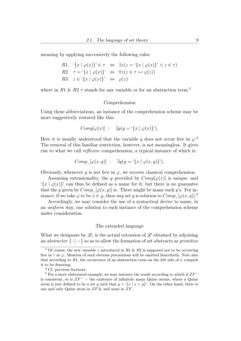
meaning by applying successively the following rules:

R1. ‘{x | ϕ(x)}’ ∈ τ ⇔ ∃z(z = ‘{x | ϕ(x)}’ ∧ z ∈ τ)

R2. τ = ‘{x | ϕ(x)}’ ⇔ ∀z(z ∈ τ ↔ ϕ(z))

R3. z ∈ ‘{x | ϕ(x)}’ ⇔ ϕ(z)

where in R1 & R2 τ stands for any variable or for an abstraction term.3

Comprehension

Using these abbreviations, an instance of the comprehension scheme may bemore suggestively restated like this:

Comp[ϕ(x)] : ∃y(y = ‘{x | ϕ(x)}’).

Here it is usually understood that the variable y does not occur free in ϕ.4The removal of this familiar restriction, however, is not meaningless. It givesrise to what we call reflexive comprehension, a typical instance of which is:

Comp� [ϕ(x, y)] : ∃y(y = ‘{x | ϕ(x, y)}’).

Obviously, whenever y is not free in ϕ, we recover classical comprehension.Assuming extensionality, the y provided by Comp[ϕ(x)] is unique, and

‘{x | ϕ(x)}’ can thus be defined as a name for it; but there is no guaranteethat the y given by Comp� [ϕ(x, y)] is. There might be many such y’s. For in-stance, if we take ϕ to be x ∈ y, then any set y is solution to Comp� [ϕ(x, y)].5

Accordingly, we may consider the use of a syntactical device to name, inan uniform way, one solution to each instance of the comprehension schemeunder consideration.

The extended language

What we designate by Lτ is the actual extension of L obtained by adjoiningan abstractor {· | −} so as to allow the formation of set abstracts as primitive

3 Of course, the new variable z introduced in R1 & R2 is supposed not to be occurringfree in τ or ϕ. Mention of such obvious precautions will be omitted henceforth. Note alsothat according to R1, the occurrence of an abstraction term on the left side of ∈ compelsit to be denoting.

4 Cf. previous footnote.5 For a more elaborated example, we may instance the result according to which if ZF−

is consistent, so is ZF− + the existence of infinitely many Quine atoms, where a Quineatom is just defined to be a set y such that y = ‘{x | x = y}’. On the other hand, there isone and only Quine atom in ZFA, and none in ZF .


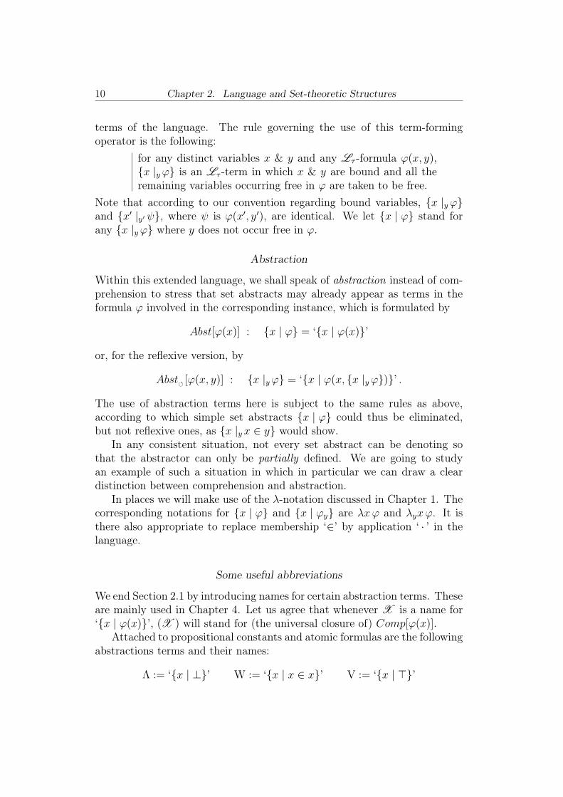
terms of the language. The rule governing the use of this term-formingoperator is the following:

for any distinct variables x & y and any Lτ -formula ϕ(x, y),{x |y ϕ} is an Lτ -term in which x & y are bound and all theremaining variables occurring free in ϕ are taken to be free.

Note that according to our convention regarding bound variables, {x |y ϕ}and {x� |y� ψ}, where ψ is ϕ(x�, y�), are identical. We let {x | ϕ} stand forany {x |y ϕ} where y does not occur free in ϕ.

Abstraction

Within this extended language, we shall speak of abstraction instead of com-prehension to stress that set abstracts may already appear as terms in theformula ϕ involved in the corresponding instance, which is formulated by

Abst[ϕ(x)] : {x | ϕ} = ‘{x | ϕ(x)}’

or, for the reflexive version, by

Abst� [ϕ(x, y)] : {x |y ϕ} = ‘{x | ϕ(x, {x |y ϕ})}’ .

The use of abstraction terms here is subject to the same rules as above,according to which simple set abstracts {x | ϕ} could thus be eliminated,but not reflexive ones, as {x |y x ∈ y} would show.

In any consistent situation, not every set abstract can be denoting sothat the abstractor can only be partially defined. We are going to studyan example of such a situation in which in particular we can draw a cleardistinction between comprehension and abstraction.

In places we will make use of the λ-notation discussed in Chapter 1. Thecorresponding notations for {x | ϕ} and {x | ϕy} are λxϕ and λyxϕ. It isthere also appropriate to replace membership ‘∈’ by application ‘ · ’ in thelanguage.

Some useful abbreviations

We end Section 2.1 by introducing names for certain abstraction terms. Theseare mainly used in Chapter 4. Let us agree that whenever X is a name for‘{x | ϕ(x)}’, (X ) will stand for (the universal closure of) Comp[ϕ(x)].

Attached to propositional constants and atomic formulas are the followingabstractions terms and their names:

Λ := ‘{x | ⊥}’ W := ‘{x | x ∈ x}’ V := ‘{x | �}’

2.1. The language of set theory 11

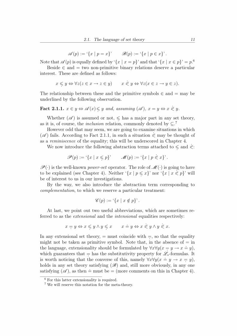
A (p) := ‘{x | p = x}’ B(p) := ‘{x | p ∈ x}’ .Note that A (p) is equally defined by ‘{x | x = p}’ and that ‘{x | x ∈ p}’ = p.6

Beside ∈ and = two non-primitive binary relations deserve a particularinterest. These are defined as follows:

x �. y ⇔ ∀z(z ∈ x → z ∈ y) x � y ⇔ ∀z(x ∈ z → y ∈ z).

The relationship between these and the primitive symbols ∈ and = may beunderlined by the following observation.

Fact 2.1.1. x ∈ y ⇔ A (x)�. y and, assuming (A ), x = y ⇔ x � y.

Whether (A ) is assumed or not, �. has a major part in any set theory,as it is, of course, the inclusion relation, commonly denoted by ⊆.7

However odd that may seem, we are going to examine situations in which(A ) fails. According to Fact 2.1.1, in such a situation � may be thought ofas a reminiscence of the equality; this will be underscored in Chapter 4.

We now introduce the following abstraction terms attached to �. and �:

P(p) := ‘{x | x �. p}’ M (p) := ‘{x | p � x}’ .

P(·) is the well-known power-set operator. The role of M (·) is going to haveto be explained (see Chapter 4). Neither ‘{x | p �. x}’ nor ‘{x | x � p}’ willbe of interest to us in our investigations.

By the way, we also introduce the abstraction term corresponding tocomplementation, to which we reserve a particular treatment:

C (p) := ‘{x | x /∈ p}’ .

At last, we point out two useful abbreviations, which are sometimes re-ferred to as the extensional and the intensional equalities respectively:

x =. y ⇔ x �. y ∧ y �. x x.= y ⇔ x � y ∧ y � x.

In any extensional set theory, = must coincide with =. , so that the equalitymight not be taken as primitive symbol. Note that, in the absence of = inthe language, extensionality should be formulated by ∀x∀y(x =. y → x

.= y),which guarantees that =. has the substitutivity property for L∗-formulas. Itis worth noticing that the converse of this, namely ∀x∀y(x .= y → x =. y),holds in any set theory satisfying (B) and, still more obviously, in any onesatisfying (A ), as then .= must be = (more comments on this in Chapter 4).

6 For this latter extensionality is required.7 We will reserve this notation for the meta-theory.


2.2 About the ground theory

As we said at the beginning, we shall be working within ZF as meta-theory.We assume all the customary practices of that set theory in the background,as the relaxed use of the ‘set of’ operator { }, etc. The reader will notice thatwe use (as much as possible) a smaller ∈ for the meta-theoretic membership.

We want to introduce here our particular notations as regards functions.We would remind the reader that set-theoretically a function f is defined byits graph, that is, the set of ordered pairs (x, f(x)). Thus functions are justparticular sets of couples, namely (binary) relations. Some special notationswill apply to relations, and then to functions.8

As usual, given a set R of ordered pairs, we write x R y for (x, y) ∈ R.The domain and the range of R are defined by domR := {x | ∃y : x R y}and rngR := domR−1, where R−1 := {(x, y) | y R x}; and given a set E, wedenote the image of E under R by R“E := {y | ∃x ∈ E : x R y}.

When f is a function, the value of f at x is denoted by f ‘x, which is thusdefined by {f ‘x} = f“{x}, so that functional application in the meta-theoryis preferably written f ‘x instead of f(x). We naturally extend this notationto list of variables, say x = x1, . . . , xn, by setting f ‘x := f ‘x1, . . . , f ‘xn. Thisis not to be confused with f ‘(x) or f(x) in case f has many variables, i.e.,when domf is a set of tuples (x) = (x1, . . . , xn). Note incidentally that wewill tacitly use all the habitual labor-saving devices in handling tuples andcartesian products. Thus, though tuples are formally defined as ordered pairsin ZF , it may be more convenient in some circumstances to look at them asfinite sequences, so that for instance we may identify the cartesian productsA× (B × C) and (A×B)× C, and then simply write A×B × C, etc.

For functional abstraction in the meta-theory, we agree that any functionf may equally be designated by x �→ f ‘x. This enables us to easily definenew functions from old. For instance, if we are given a two-variables function(x, y) �→ f ‘(x, y) and b ∈ rng(domf), then g : x �→ f ‘(x, b) will represent thefunction g = {(a, f ‘(a, b)) | a ∈ dom(domf)}.

The notation f : A −→ B means that f is a function with domf = A andrngf ⊆ B, and we denote the set of all functions f : A −→ B by (A → B).The notation β

α is reserved for exponentiation of cardinals α = |A|, β = |B|.We write A � B to indicate that two sets A and B have the same cardinal.If a particular kind of structure has been specified on these and we want toexpress that they are isomorphic in the corresponding category of structuredsets, we write A ∼= B. Thus � does correspond to ∼= in the category of puresets, which we call SET .

8 These notations may apply as well to relations and functions that are proper classes.

2.3. Set-theoretic structures 13

There is a correspondence in SET that is worth making explicit, namelythe canonical bijection between the power-object P(A) and the exponential

(A → 2), where 2 = {0, 1}. It will be designated by ıA : P(A) −→ (A → 2)and its inverse by A : (A → 2) −→ P(A), i.e.

for any E ∈ P(A), ıA‘E : x �−→ 1 if x ∈ E

0 otherwise

and

for any f ∈ (A → 2), A‘f := {x ∈ A | f ‘x = 1} .

Although they are isomorphic in SET , there is a difference from the categor-ical point of view between P(A) and (A → 2), in that the endofunctor P(·)is covariant whereas (·→ 2) is contravariant : when F(·) is P(·) the actionof F(·) on f : A −→ B is defined by f

F : P(A) −→ P(B) : E �−→ f“E;when F(·) is (·→ 2) it is given by f

F : (B → 2) −→ (A → 2) : h �−→ h ◦ f .Thus (g ◦ f)F = g

F ◦ fF in the first case, whereas (g ◦ f)F = f

F ◦ gF in the

second. (As usual, we use ‘◦’ for composition of functions or relations.)

2.3 Set-theoretic structuresHere we present different ways of modelling a set-theoretic structure. As thatwill be illustrated throughout this thesis, one view may prove more suitablethan another depending on the context. We also have a look at correspondinghomomorphisms and the formulas they preserve.

Structures

As an L -structure, a set-theoretic universe U is regarded as

�U ;∈U� where ∈U ⊆ U × U (U �= ∅).

But if a set is to be conceived of as the collection of its members, the followingequivalent presentation is arguably more natural:

�U ; [·]U � where [·]U : U −→ P(U)v �−→ {u ∈ U | u∈U v}.

We call [y]U the extension of y in U .9

9 It is worth stressing the difference between Frege’s definition of the extension of aconcept, which is the corresponding set as object, and the extension of a set in a givenstructure as defined here.


We now display the notations for the valued counterparts of these settings:

�U ; �U� where �U : U × U −→ 2

and

�U ; [[·]]U � where [[·]]U : U −→ (U → 2)v �−→ (u �→ �U ‘(u, v)) .

Explicitly, �U = ıU×U ‘∈U and [[v]]U = ıU ‘[v]U for every v ∈ U .Unless otherwise stated, the interpretation of the equality relation in a

structure is taken to be the identity, i.e.

∆U := {(u, v) ∈ U × U | u = v} / δU := ıU×U ‘∆U : (u, v) �−→ 1 if u = v

0 otherwise.

This canonical interpretation may not always be appropriate (as illustratedin Chapter 6). Nevertheless, it is well known that any structure with anacceptable interpretation of = can be contracted to a normal one, that is,one in which = is the identity.10 As far as extensionality is concerned, theextension function [·]U/[[·]]U is injective when U is normal.

Language in structures

As previously mentioned, given a structure U , we conveniently extend thelanguage by the elements of U seen as constants; this extended language isdesignated by L (U) or Lτ (U). For this latter we will use the λ-notationwhenever structures are being looked at in the valued setting(s).

We denote the truth-value of a formula ϕ(p) interpreted in U , for theassignation p := u in U , by |ϕ(u)|U . The interpretation of a term τ(p) withina structure U , for p := u in U , is designated by τU(u).

What is needed to turn an L -structure into an Lτ -one is the interpre-tation of the abstractor wherever it is defined, and this actually depends onthe fragment of Lτ under consideration.

Besides being subject to satisfying the corresponding instances of ab-straction, the interpretation of {· | −} in a structure U has to fulfil a naturalsubstitutivity property. Namely, for any Lτ -formula ϕ(x, p) and list of Lτ -terms τ(q) of the same length as p, it is required that, whenever all the termsinvolved are defined, the following equality hold:

U |= {x | ϕ}U(τU(u)) = {x | ψ}U(u)

10 By an ‘acceptable’ interpretation of = we mean one that ensures the substitutivityproperty for formulas and terms of the language under consideration.

2.3. Set-theoretic structures 15

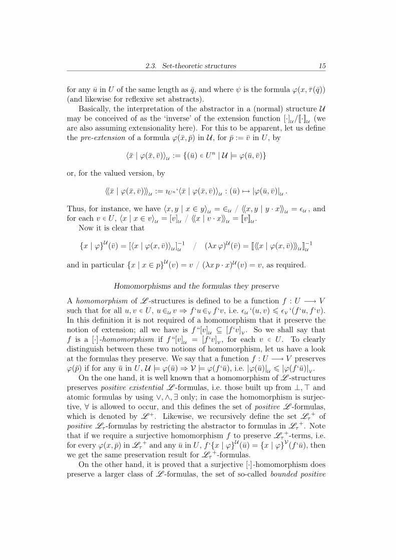
for any u in U of the same length as q, and where ψ is the formula ϕ(x, τ(q))(and likewise for reflexive set abstracts).

Basically, the interpretation of the abstractor in a (normal) structure Umay be conceived of as the ‘inverse’ of the extension function [·]U/[[·]]U (weare also assuming extensionality here). For this to be apparent, let us definethe pre-extension of a formula ϕ(x, p) in U , for p := v in U , by

�x | ϕ(x, v)�U := {(u) ∈ Un | U |= ϕ(u, v)}

or, for the valued version, by

��x | ϕ(x, v)��U := ıUn ‘�x | ϕ(x, v)�U : (u) �→ |ϕ(u, v)|U .

Thus, for instance, we have �x, y | x ∈ y�U = ∈U / ��x, y | y · x��U = �U , andfor each v ∈ U , �x | x ∈ v�U = [v]U / ��x | v · x��U = [[v]]U .

Now it is clear that

{x | ϕ}U(v) = [�x | ϕ(x, v)�U ]−1U

/ (λxϕ)U(v) = [[��x | ϕ(x, v)��U ]]−1U

and in particular {x | x ∈ p}U(v) = v / (λx p · x)U(v) = v, as required.

Homomorphisms and the formulas they preserve

A homomorphism of L -structures is defined to be a function f : U −→ V

such that for all u, v ∈ U , u∈U v ⇒ f ‘u∈V f ‘v, i.e. �U ‘(u, v) � �V ‘(f ‘u, f ‘v).In this definition it is not required of a homomorphism that it preserve thenotion of extension; all we have is f“[v]U ⊆ [f ‘v]V . So we shall say thatf is a [·]-homomorphism if f“[v]U = [f ‘v]V , for each v ∈ U . To clearlydistinguish between these two notions of homomorphism, let us have a lookat the formulas they preserve. We say that a function f : U −→ V preservesϕ(p) if for any u in U , U |= ϕ(u) ⇒ V |= ϕ(f ‘u), i.e. |ϕ(u)|U � |ϕ(f ‘u)|V .

On the one hand, it is well known that a homomorphism of L -structurespreserves positive existential L -formulas, i.e. those built up from ⊥,� andatomic formulas by using ∨,∧,∃ only; in case the homomorphism is surjec-tive, ∀ is allowed to occur, and this defines the set of positive L -formulas,which is denoted by L +. Likewise, we recursively define the set Lτ

+ ofpositive Lτ -formulas by restricting the abstractor to formulas in Lτ

+. Notethat if we require a surjective homomorphism f to preserve Lτ

+-terms, i.e.for every ϕ(x, p) in Lτ

+ and any u in U , f ‘{x | ϕ}U(u) = {x | ϕ}V(f ‘u), thenwe get the same preservation result for Lτ

+-formulas.On the other hand, it is proved that a surjective [·]-homomorphism does

preserve a larger class of L -formulas, the set of so-called bounded positive


formulas, denoted by L [+], in which bounded quantifications of the form‘∀x ∈ y’ are permitted too.11 As a distinguished member of L [+], we quotethe formula p �. q, and so p =. q. Given a [·]-homomorphism f : U −→ V ,let us show that if ϕ(x, p) is preserved under f , so is ∀x(x ∈ pk → ϕ(x, p)),where pk is in p.

Proof. Assume that ϕ(x, p) is preserved and that U |= ∀x(x ∈ uk → ϕ(x, u)),for u given in U (uk in u). Let v ∈ V such that v ∈V f ‘uk, that is, v ∈ [f ‘uk]V .As f is a [·]-homomorphism, we can find u� ∈ [uk]U such that f ‘u� = v. Now,from u� ∈U uk, we get U |= ϕ(u�, u), and as ϕ(x, p) is preserved, we haveV |= ϕ(v, f ‘u). Whence V |= ∀x(x ∈ f ‘uk → ϕ(x, f ‘u)). �

We have thus introduced the classes L +/Lτ

+/L [+] in a natural way by

looking at formulas that are preserved under projections. In the next chapterwe will review what is known on comprehension/abstraction restricted tothese classes of formulas.

To give a complete account, we now conclude this section by a couple ofremarks related to homomorphisms again.

Remark 2.3.1. Assume we are given a set-theoretic structure U together withan equivalence relation R on U . There is a natural way to try to define anotion of extension on the quotient set V := U/R. Namely, we define [f ‘v]Vto be f“[v]U , where f : U −→ V : u �−→ R“{u} is the corresponding pro-jection map. In order for this to work, it is necessary that for all v, v� ∈ U ,v R v

� ⇒ R“[v]U = R“[v�]U , and as R is an equivalence relation, this amountsto v R v

� ⇒ [v]U ⊆ R“[v�]U . In theoretical computer science an equiva-lence relation R on U satisfying this condition is called a (bi)simulation.It is now apparent that bisimulations are exactly kernels of surjective [·]-homomorphisms (where the kernel of a map f is as usual the equivalencerelation R on domf defined by u R v if and only if f ‘u = f ‘v).

Remark 2.3.2. The reader familiar with category theory will have noticedthat our notions of [·]/[[·]]-structures are particular cases of coalgebras : givena category CAT and an endofunctor F acting on CAT , a F-coalgebra isdefined to be any object U together with a morphism s : U −→ F(U). Thus,within the category SET , [·]-structures and [[·]]-structures are just P(·)-coalgebras and (·→ 2)-coalgebras respectively. Coalgebras form a category:a F-morphism between F -coalgebras �U ; s� and �V ; t� is given by a morphismf : U −→ V with a natural commutativity property. As far as F is covariant,this condition is t◦f = fF◦s. In the case where F is contravariant, it should

11 This is no longer true for ‘∀x ∈ x’. On the other hand, bounded quantifications of theform ‘∃x ∈ y’ and ‘∃x ∈ x’ are also preserved since these are actually positive.

2.4. Models for set theory 17

be expressed by fF◦t◦f = s. It follows that the notion of P(·)-morphism and

the one of (· → 2)-morphism differ. What we called a [·]-homomorphism isnothing but a P(·)-morphism, which was thus characterized by the condition[f ‘v]V = f“[v]U , for every v ∈ U . In these terms, it is easily seen that thecorresponding condition for f to be a (· → 2)-morphism would correspondto f−1“[f ‘v]V = [v]U , for each v ∈ U , which is clearly a strong requirementfor it is equivalent to u∈U v ⇔ f ‘u∈V f ‘v, for any u, v ∈ U . We might callsuch a function f : U −→ V a [[·]]-homomorphism. When f is injective,this is known as an embedding ; when f is surjective, it is in particular a[·]-homomorphism. Note that it is hopeless to obtain consistency results forformulas preserved under [[·]]-homomorphisms since x /∈ x is one of these.

2.4 Models for set theoryGiven a set-theoretic structure U , rng[·]U is nothing but the set of collectable

subsets of U . We now define def[·]U to be the set of definable subsets of U , i.e.def[·]U := {�x | ϕ(x, v)�U | ϕ(x, p) in L , v in U}. Note that rng[·]U ⊆ def[·]U .

Russell’s paradox says that, in any case, �x | x /∈ x�U /∈ rng[·]U , from whichit follows that rng[·]U � P(U) (Cantor’s theorem). This is not an accident forit can be shown that actually |def[·]U \ rng[·]U | = |U | if U is infinite (see [22]),and, more obviously, that |P(U) \ rng[·]U | > |U | unless |U | = 1 or 2. So weare very far from the idealistic Fregean situation U � P(U) /U � (U → 2).

In every model U of any extensional set theory, the set of collectablesubsets must have the same size as U . Some set theory might thus be char-

acterized in some of its models by the selection of a specific class of subsetsF(U) such that U � F(U). As a famous example, we may quote ZF .

Limitation of size

Given a set U and a cardinal κ, we let P<κ(U) stand in what follows for theset of κ-finite subsets of U , i.e. {A ⊆ U | |A| < κ}.

Within ZF as framework, it is proved that there exists one and only setU such that U = P

<ℵ0(U), namely U = Vω, which is precisely known to be

a model of ZF �∞ (here [·]U is just taken to be the identity function).12 Andif one wants a model of infinity as well, this is still possible by invoking the

12 As the notation suggests, ZF �∞ stands for ZF without the Axiom of Infinity. Bythe way, we would also remind the reader of the definition of the Vα’s, α an ordinal:Vβ+1 := P(Vβ), for any β, and Vλ := {Vγ | γ < λ}, if λ is a limit ordinal. Notice that theaxioms of ZF− are just formulated in order that this construction, the so-called cumulativehierarchy, can be achieved; in ZF , the universe does coincide with {Vα | α ordinal}.


existence of a strongly inaccessible cardinal κ, so that Vκ , which is the solesolution in ZF to U = P<κ(U), is itself a model of ZF .

It is worthy of note that if the meta-theory is ZFA, there are differentsuch U ’s: the minimal one is still Vκ, model of ZF , and the maximal one isnow itself a model of ZFA (idem when κ = ℵ0 but we lose infinity).

So we have indeed a situation here in which a model for some set theory,which is ZF/ZFA, arises from a bijection - the identity as it is - betweena set U and a set of distinguished subsets of U , namely the κ-finite subsets.Furthermore, the existence of these canonical models perfectly shows thatZF is just the theory of hereditarily small and iterative sets; as for ZFA,we simply drop the adjective ‘iterative’. It is the reason why the guidingprinciple of ZF/ZFA for avoidance of the paradoxes is often referred to asthe so-called limitation of size doctrine.

Adding structure

A natural way of specifying a class of subsets of a given set consists in addingsome structure on it and then looking at particular subsets which are definedin terms of the underlying structure. The previous example falls into this inan obvious way: if Vω is regarded as a topological space with the discretetopology, the finite subsets are just the compact ones, so Vω now appears asa topological solution U to U � Pcpact(U), the set of compact subsets of U .

Viewing things that way has at least the merit of suggesting a moreinteresting situation, in which the underlying topology on U would be suchthat U itself be compact, so that this latter would be collectable, and sothere would be a universal set. In fact, it was shown that such a compact

solution to U � Pcpact(U) exists.13 More precisely, it is proved that withina suitable category of T2-spaces there is one (and only) compact solution Uto U ∼= Pcl(U), the set of closed subsets of U - endowed with a suitabletopology. It was called Nω.

A very characteristic property of the corresponding set-theoretic struc-ture, which is actually shared by any solution U to U � Pcl(U), is thus thefollowing: every class ‘{x | ϕ(x)}’ can be approximated by a least upper set,the extension of which is just the closure of �x | ϕ(x)�U in U . This propertyis explicitly formulated in Chapter 4 where it is referred to as (✸).

Interestingly, it turns out that the set-theoretic structure associated withNω is also a model of Comp[ϕ(x)] for every ϕ(x) in L [+], which is a syntactical

fragment of L - whereas the axioms of ZF are not. It is all the more inter-esting in that it is shown in [12] that the first-order theory (✸)+Comp[L [+]],

13 Within ZFA as framework we may even write U = Pcpact(U).

2.4. Models for set theory 19

which was named GPK+ for historical reasons, can interpret ZF �∞ in a nat-

ural way. And in order to interpret ZF , it suffices to add to GPK+ an

axiom ensuring the existence of the least infinite Von Neumann ordinal ω,which yields the theory GPK

+∞ deeply investigated in [12]. Note that it was

originally proved in [17] that with a large cardinal assumption - namely theexistence of a weakly compact cardinal - the technique used to construct Nω

can be so carried out as to fulfil that relevant axiom of infinity.

Topological solutions

In light of what has been said, we may define a topological model for set theoryto be any set-theoretic structure U that is solution to an equation U � F(U),or even better U ∼= F(U), where F(·) is some power-object/exponential act-ing on a category of topological spaces. Typically, one may think of F(U)to be Pcl(U), the set of closed subsets of U , or Pop(U), the set of open ones,both endowed with some suitable topology if required. It is worth emphasiz-ing that by a solution U we really mean a topological space U together with

a bijection / homeomorphism ‘[·]U’ realizing U � F(U) /U ∼= F(U).In such set-theoretic structures it might be said that it is the indiscerni-

bility associated with the underlying topology that governs the collectingprocess. And that such equations can be solved within suitable categoriesof topological spaces would thus mean that, to some extent, the Fregeanproblem is solvable under indiscernibility.

As we shall see, however, we are still far from the idealistic Fregean per-spective. Indeed, in most cases the axiomatic set theory to which topologicalmodels give rise is rather insignificant in itself from the foundational pointof view. In fact, the sole exception we know is our guiding example above.14

Anyway, we are not seeking a new proposal in this thesis. We are onlyinterested in consistency results on comprehension/abstraction restricted tosome syntactical fragments of L /Lτ . The next chapter is precisely intendedto show how topological considerations then naturally come into the picture.

14 It is shown in [12] that GPK+∞ is as strong as ‘Kelley-Morse + On is ramifiable’.

Chapter 3

CONTINUITY:A SAFETY PROPERTY

Here we make a survey of various proposals which are closely related to ourinvestigations. The content of this chapter is to appear in [29].

3.1 Deviation in logicIt must be admitted that mathematical investigations in providing alternative

semantics have carried innovative ideas, and if all have not led to furtherdevelopments and applications, they have often led to a better understandingof the topic considered.

Even within a well-established framework, the use of alternative semanticshas proved its fruitfulness. As an example, for independence results in ZF ,one may quote the Boolean-valued version of forcing due to Scott and Solovay,in which a set is conceived of as a function that takes its values into a givencomplete Boolean algebra, no more into the 2-valued one. This concernsclassical logic and perhaps would remind the reader of the primal use of many-valued semantics for proving the independence of axioms in propositionallogic. Note that there is no need to be interested in any possible meaningof the additional ‘truth values’ to do that. We would rather say that theexplanation is in the application.

Now, it is legitimate to enquire whether the use of many-valued semanticsand the like could not also benefit, in one way or another, our understandingof the set-theoretical paradoxes. After all, to know which logical systems

whatsoever can support the full comprehension scheme, or some fragmentsof it, is an interesting question in itself, at least not devoid of mathematicalinterest. We would then let the various proposals speak for themselves.

As said in Chapter 1, we shall be concerned with type-free approaches inthis thesis, and mainly with those that somehow reject classical negation.1

1 For a solution route in which the definition of ≡ is altered, while classical negation is

22 Chapter 3. Continuity: A Safety Property

So we review in this chapter some attempts in that direction, giving anhistorical account on the subject in connection with the pioneering work ofSkolem in Łukasiewicz’s logics. Our aim is to trace and stress the use offixpoint arguments in semantic consistency proofs and, thereby, the role ofcontinuity in avoiding the paradoxes. It will then become apparent how closethese investigations were to other contemporary ones, as Kripke’s seminalwork on the liar paradox and Scott’s on models for the untyped λ-calculus.We also aim to show how the distinction comprehension/abstraction and theexistence of topological models - both of which being explored in this thesis- have emerged from such ‘deviant’ proposals.

3.2 Moh Shaw-Kwei’s paradoxThe existence of the Russell set is prohibited in classical logic. By tamperingwith the negation, some alternative logics have proved more tolerant. Never-theless, there exist other sets that can affect such non-classical systems. Thiswas illustrated in 1954 by Moh Shaw-Kwei [32] who presented the followingextended version of Curry’s paradox.

Let → be the official implication connective of the logic considered. Pre-cisely, in order that → may be referred to as an implication connective, it isassumed that modus ponens holds, namely

MP : ϕ , ϕ → ψ � ψ

where � is the consequence relation associated with the logic.To express Moh’s paradox, we define the n-derivative →n of the implica-

tion inductively as follows:

ϕ →0ψ :≡ ψ and ϕ →n+1

ψ :≡ ϕ → (ϕ →nψ) (n ∈ N).

Then the implication connective is said to be n-absorptive if it satisfies theabsorption rule of order n, that is,

An : ϕ →n+1ψ � ϕ →n

ψ.

Now, assuming that the implication is n-absorptive for some n > 0, itis easily seen that any formula can be derived from the existence of the setCn := ‘{x | x ∈ x →n⊥}’, where ⊥ is a ‘falsum’ constant defined in such away that ⊥ � ϕ, for any ϕ.

maintained, the reader is referred to [3].

3.3. The Łukasiewicz logics 23

Proof.

Comp[L ] � ∀x ( x ∈ Cn ↔ (x ∈ x →n⊥) ) [Comprehension] (1)� Cn ∈ Cn ↔ (Cn ∈ Cn→n⊥) [Univ. Quant. Elimin.] (2)� Cn ∈ Cn→n⊥ [(2)→ , An] (3)� Cn ∈ Cn [(2)← , (3), MP ] (4)� ⊥ [(3), (4), MP (n times)] (5).

Thus any formula can be derived and the theory is meaningless. �

As a particular case we have C1 = ‘{x | x ∈ x → ⊥}’, which might becalled the Curry set, and then we recover the Russell set R = ‘{x | x /∈ x}’ if¬ϕ is defined by ϕ → ⊥, as it is the case in classical logic. Note incidentallythat C0 = ‘{x | ⊥}’, but this later is not problematic, of course.

3.3 The Łukasiewicz logicsA nice illustration is supplied by the most popular many-valued logics, theŁukasiewicz ones. We shall content ourselves here with recalling the truth-functional characterization of the connectives and quantifiers of these logics.

The set of truth values for the infinite-valued Łukasiewicz logic Ł∞ istaken to be the real unit interval I := [0, 1] ⊆ R with its natural ordering,which will be referred to as the truth ordering and denoted by �T . The soledesignated value is 1. Here are the truth functions of the logical operators:2

◦ ⊥ is 0 and � is 1;

◦ negation is defined by ¬x := 1− x, for any x ∈ I;

◦ conjunction and disjunction are the minimum and maximum w.r.t. �T ,i.e., x ∧ y := min�T

{x, y} and x ∨ y := max�T{x, y}, for any x, y ∈ I;

◦ quantifiers are thought of as generalized conjunction and disjunction,i.e., for any A⊆I, ∀A := inf�T

A and ∃A := sup�TA;

◦ last but not least, the truth function of the implication is specificallydefined by x → y := min�T

{1, 1 − x + y}. Notice that this is not the‘material conditional’ x ⊃ y := ¬x∨ y ; we only have x ⊃ y �T x → y.Thus defined, → is a characteristic function of the truth ordering, forwe have x → y = 1 if and only if x �T y, which ⊃ fails to fulfil here.Consequently, ≡, which is just taken to be ↔, is still characterized byx ≡ y = 1 if and only if x = y. That is to say, U |= ϕ ≡ ψ if and onlyif |ϕ|U = |ψ|U , as in classical logic.

2 We use the same notation for the operators and their truth functions.


For our purposes, we remark that if we equip I with the usual topology ofthe real line, then each of the truth functions of the connectives is continuous.The truth functions of the quantifiers are continuous as well with respect toa reasonable topology on the set of subsets of I. This extra-logical propertyof the interpretation of the logical operators will be of interest to us.

The n-valued Łukasiewicz logic Łn (n � 2) is obtained by restricting theset of truth values to In := { k

n−1 | k ∈ n}. Particular cases are then the 2-valued logic Ł2, which is nothing but classical logic, and the 3-valued one Ł3,which historically was the first many-valued logic introduced by Łukasiewicz.

It was noticed in [32] that the implication is (n−1)-absorptive in Łn,whereas it is not n-absorptive in Ł∞, for any value of n, whereupon theauthor asked whether one could develop the naive theory of sets from Ł∞.

3.4 Skolem’s conjecture

This observation was the starting point in the late fifties of a course of papersinitiated by Skolem, who conjectured and tried to prove in [35] the consis-tency of the full comprehension scheme in Ł∞.3 On the way, Skolem was ledto considering and investigating the consistency problem of some fragmentsof that scheme in Ł3 & Ł2 [36, 37, 38], on which we are going to dwell later.

Skolem’s conjecture was partially confirmed by Skolem himself in [35]and by Chang and Fenstad in different papers [10] & [15]. For instance,Skolem only showed the consistency of the comprehension scheme restrictedto formulas containing no quantifiers, while Chang had quantifiers but noparameters, or parameters but then some restrictions on quantifiers.

From the technical point of view, what should be said is that all thesefirst attempts are semantic and that their proofs are based on the originalmethod of Skolem, using at some stage a fixpoint theorem, namely Brouwer’s

fixpoint theorem for the space Im, m ∈ N (or even for I

N), which statesthat any continuous function on I

m (or IN) has a fixpoint. We will meet

another famous fixpoint theorem which was also used, but rather implicitly,in Skolem’s papers [36, 37].

We shall show in 3.6 how fixpoint arguments can be involved in suchsemantic consistency proofs. Let us first see what a many-valued set-theoreticstructure looks like.

3 As just mentioned, this suggestion was made by Moh Shaw-Kwei in [32]. It shouldbe remarked however that Skolem does not cite that work. He might have arrived at hisconclusions independently.

3.5. Many-valued structures 25

3.5 Many-valued structuresA set-theoretic structure U for a many-valued logic of which T is the set oftruth values is defined like the 2-valued classical version(s) presented in 2.3:

�U ; �U� where �U : U × U −→ T

or

�U ; [[·]]U � where [[·]]U : U −→ (U → T )v �−→ (u �→ �U ‘(u, v)).

In the case of Ł2, we noticed in 2.3 that a normal structure U is extensional

if and only if [[·]]U is injective. But in the case of Ł∞ / Łn, n > 2, what it is fora structure to be extensional is not so clear, for the principle of extensionalityitself may be subject to different interpretations. This is because in Ł∞ / Łn,n > 2, the implication → is no longer the translation at the object-languagelevel of the consequence relation � (only Modus Ponens remains). Therefore,depending on whether it is considered as a rule or as an axiom, and dependingalso on whether equality is taken as primitive or not, different versions ofextensionality are conceivable (note that ‘�’ has no effect in Ł2):

�Ext : x =. y � x

.= y�Ext

� : � ∀x∀y(x =. y → x.= y)

Ext : x =. y � x = y Ext� : � ∀x∀y(x =. y → x = y).

In order for = to bear the title of equality, it is to be required that it beso interpreted in any structure as to guarantee the principle of substitutivity

(again, either as a rule or as an axiom scheme). This can be met by simplydefining the truth function of = on any structure by =U ‘(u, v) := 1 if and onlyif u = v in U , and =U ‘(u, v) := 0 otherwise. Incidentally, it was noticed in [10]that this strict interpretation will never yield a model of Comp[L ] + Ext

�.A more reasonable definition of the equality relation in a structure may beany one such that =U ‘(u, v) = 1 if and only if u = v in U , and that is all,for this suffices to ensure that = has the substitutivity property (but as arule, not as an axiom scheme actually). Any structure equipped with suchan interpretation of = will be said to be normal. In that case, it is easy tosee that [[·]]U is injective if and only if U is extensional in the sense of Ext.This latter shall henceforth be our preferred version of extensionality.

Accordingly, the universe U of any extensional normal structure U maybe identified with a (proper) subset of (U → T ), namely the range of [[·]]U ,so that U now appears as a solution to U � [U → T ], where [U → T ] is asuitable set of functions U −→ T , or say, a set of suitable functions U −→ T .


Of course, because of Cantor’s theorem, not every function U −→ T issuitable. Worse, even some simple propositional truth-functions may not be.As we shall now see, only truth-functions having fixpoints are welcome.

3.6 The fixpoint property

Let A(·) be any propositional function in one variable, and let α : T −→ T

denote its truth-function. Now suppose we are given a set-theoretic structureU in which ‘{x | A(x ∈ x)}’ has an interpretation, say a ∈ U . Then we musthave |a ∈ a|U = |A(a ∈ a)|U = α(|a ∈ a|U ), showing that α : T −→ T has afixpoint, namely |a ∈ a|U . We shall refer to this as the fixpoint property. Itfollows therefrom that if ever U |= Comp[L ], then any propositional truth-function α : T → T must have the fixpoint property.

In the case of Łn, n � 2, not every propositional truth-function can havethe fixpoint property. An example was actually provided in the proof ofMoh Shaw-Kwei’s paradox. Indeed, just take α(x) := x→n⊥. A simplecomputation shows that α(x) = min�T

{1 , n(1− x)}, from which it is easilyseen that α has no fixpoint on In.

On the other hand, in the case of Ł∞, the fixpoint property is fulfilled.For we noticed in 3.3 that the truth-functions of the logical connectives andquantifiers of Ł∞ are continuous, and then so is any truth-function α : I −→ I

defined from these. Now, by Brouwer’s theorem, any such α has a fixpoint. Itis then not surprising that the Brouwer fixpoint theorem was involved in thefirst attempts to provide a model of Comp[L ] in Ł∞. Broadly, this examplewould even suggest that continuity, in a very comprehensive manner as weshall see, might be regarded as a safety property against the paradoxes.

3.7 White’s solution

The use of an abstractor within a many-valued framework is conceivable too.And it was precisely by using an abstraction operator, and by a proof-theoretic

method in fact, that Skolem’s conjecture was finally established much later byWhite in 1979 ; see [41]. What was actually proved therein is the consistencyof Abst[Lτ ∗] in Ł∞. It was noticed by the author himself that his system is tooweak in order to develop classical first-order number theory inside. He alsoshowed that �Ext� cannot be consistently added, but we ignore whether �Ext

can be. In fact, it is still not known whether Comp[L ] + Ext is consistent.If so, any semantic proof showing the existence of natural models would be

3.8. Abstraction and extensionality 27

welcome in that such models would give rise to a full universe of fuzzy sets.4We now leave the consistency problem of the full comprehension scheme

in Ł∞, and concentrate on the one of some syntactical fragments of it inŁ3 and Ł2, as initiated by Skolem in [36, 37, 38]. Although the use of setabstracts in the language was again salutary to prove their consistency, weare going to see that it can also be fatal to extensionality in the presence ofequality in formulas defining sets.

3.8 Abstraction and extensionalityAssuming extensionality, set abstracts can be eliminated. But in doing that,some undesirable connectives may sneak in by the back door. This is partic-ularly well illustrated by the rule R2 stated in 2.1:

τ = ‘{x | ϕ(x)}’ ⇔ ∀z(z ∈ τ ↔ ϕ(z)) ,

the following instance of which is still more eloquent

‘{x | ⊥}’ = ‘{x | ϕ(x)}’ ⇔ ∀z(⊥ ↔ ϕ(z)) ⇔ ¬ϕ (†).

Now it is easily proved that, assuming Ext, the Russell set can be definedin Ł2 without negations or implications, simply by using set abstracts andequality in the language. This results in the key observation that follows:

Fact 3.8.1. Abst[Lτ+] is incompatible with Ext

Proof. Assume Abst[Lτ+] and define r := {x | {z | x ∈ x} = {z | ⊥}}.

Assuming Ext, it follows from (†) that r = ‘{x | x /∈ x}’. �

This sort of ‘paradoxes’ first appeared in Gilmore’s work on partial settheory [19].5 It should be remarked that the Russell set is no longer contra-dictory in Gilmore’s set theory. What was showed in [19] is that, within anextensional universe, a substitute for it can be defined by using set abstractsand equality in the language, in a similar (yet more subtle) manner as above.

Although his motivations were elsewhere, that work by Gilmore couldhave equally been expressed within the 3-valued Łukasiewicz logic. As amatter of fact, Brady in [8] directly adapted Gilmore’s technique to Ł3 to

4 So far we have only obtained partial results, comparable to those of [10] & [15], byusing techniques described in [4]. This should be discussed elsewhere.

5 It is worthy of note that Gilmore’s work was first publicized in 1967, but the incon-sistency of extensionality only appeared in 1974.


much strengthen Skolem’s initial result, showing the consistency of an ab-straction scheme in that logic, but without equality in the language (as inSkolem). By this mere fact, however, a significant departure in [8] is that theauthor succeeded in proving that his model is extensional, and thus, thoughhe was not aware of that,6 he actually proved a complementary result ofGilmore’s. Namely, one can recover extensionality by dropping equality outof formulas defining sets.

To clearly express those results of Gilmore and Brady, let Lτ�→ stand

for the set of Lτ -formulas containing no occurrences of →. Notice that thisrestriction is meaningful in view of Moh Shaw-Kwei’s paradox. Then we have

Theorem ([19]).Abst[Lτ

�→] is consistent in Ł3, but inconsistent together with Ext.


�→∗ ] + �Ext is consistent in Ł3.

We mention here that similar results apply as well to the paraconsistent

counterpart of Ł3, the quasi-relevant logic RM3 (e.g. in [9]). For a survey ofthe paraconsistent approach, we refer the reader to [27].

Before Gilmore/Brady’s method, Skolem had built extensional models ofa comprehension scheme in Ł3 restricted to formulas not containing any oc-currence of →, but not any quantifier either (and without equality in thelanguage). In fact, his technique of proof in [36, 37] cannot be extended inorder to handle quantifiers. But Skolem showed in [37] that it can be adaptedto Ł2, initiating by the way, as far as we know, the consistency problem forpositive comprehension principles. Moreover, he presented different tech-niques in [37] and [38], one of which finally led him to prove the consistencyof Comp[L +

∗ ]+Ext (see [38], Theorem 1). The model he discovered is goingto be further analyzed in Chapter 5, where all its secrets will be revealed.

Without any references to Skolem, the consistency problem for positivecomprehension principles was reinvestigated and invigorated much later inthe eighties, where it would seem to have his source in Gilmore’s work pre-cisely; see [21] & [17]. Then it is not surprising that similar results to thosestated for Ł3 could be proved for Ł2.


+] is consistent in Ł2, but inconsistent together with Ext.


+∗ ] + �Ext is consistent in Ł2.

6 Cf. previous footnote.

3.9. A particular case of continuity 29

But here much more interesting extensional models were actually discov-ered in order to recover equality in formulas defining sets, and thus by givingup the use of set abstracts.

Theorem ([17]).Comp[L +] + Ext is consistent in Ł2.

We also mention that the technique used to construct them was subse-quently adapted by Hinnion in [23] to the partial and the paraconsistentcases with different success (see also [28, 27] for the paraconsistent version).

The rest of this chapter is in a sense devoted to showing how such modelscan be obtained. To proceed, we first have to point out the guiding idea,which was already subjacent in the original work of Skolem.

3.9 A particular case of continuityThe key step in Skolem’s proofs of the consistency of a comprehension schemein Ł3 and Ł2 (see [36] and [37]) is again the observation that the truth func-tions of formulas defining sets have the fixpoint property. Of course, as theset of truth values is discrete, it is no longer possible to invoke Brouwer’s the-orem to see that. As a matter of fact, Skolem contents himself in [36] withnoticing that there are exactly eleven propositional truth-functions in onevariable constructible in Ł3 without using →, and that each of them reallyhas a fixpoint. In [37] a similar remark for positive formulas is applied to Ł2.Although this was not noticed by Skolem, it is another famous fixpoint the-orem that is hidden behind these observations, namely the Knaster-Tarski

theorem for ordered sets, on which we shall now dwell.We would remind the reader that a particular case of continuity is mono-

tonicity. For it is well known that if any (partially) ordered set is endowedwith the topology for which the open subsets are just the upper sets, i.e.,A is open if and only if x � a ∈ A ⇒ x ∈ A, then the continuous functionsare exactly the monotone ones. This technically convenient topology is re-ferred to as the Alexandroff topology. It may be defined on any preordered

set actually, and it is easily characterizable as we shall see later in 4.7.Now it turns out that the ordered sets on which any continuous/monotone

function has a fixpoint are identifiable. These are the dcpo’s.We say that an ordered set U is directed complete, or a dcpo for short,

if any directed subset of U has a least upper bound, denoted by A; whereD ⊆ U is said to be directed if D �= ∅ and for any a, b ∈ D, there exists c ∈ D

with a, b � c. If in addition ∅ exists, that is to say, if U has a least element,then we say that U is a pointed dcpo (some authors use the term cpo).


Any complete ordered set is obviously a pointed dcpo, and the relevanceof this notion lies in the following important theorem, which is in fact thebest refinement of Tarski’s original version for complete lattices:

Theorem (Knaster-Tarski).Let U be a pointed dcpo and let f : U −→ U be monotone. Then Fix(f),the set of all fixpoints of f , is itself a pointed dcpo. Consequently, f has a

(least) fixpoint. Moreover, if U is a complete lattice, so is Fix(f).

We denote the least fixpoint of f by µ(f). Using the machinery of ordi-nal numbers, µ(f) can be reached inductively by iterating f from the leastelement of U (whereas the existence of maximal ones relies on Zorn’s lemma,unless U is a complete lattice or is finite, of course).

To complement the Knaster-Tarski theorem, it has been shown that a

(pointed) ordered set on which any monotone function has a fixpoint is nec-

essarily a dcpo. This is, by far, much more difficult to prove (see [1] forreferences).

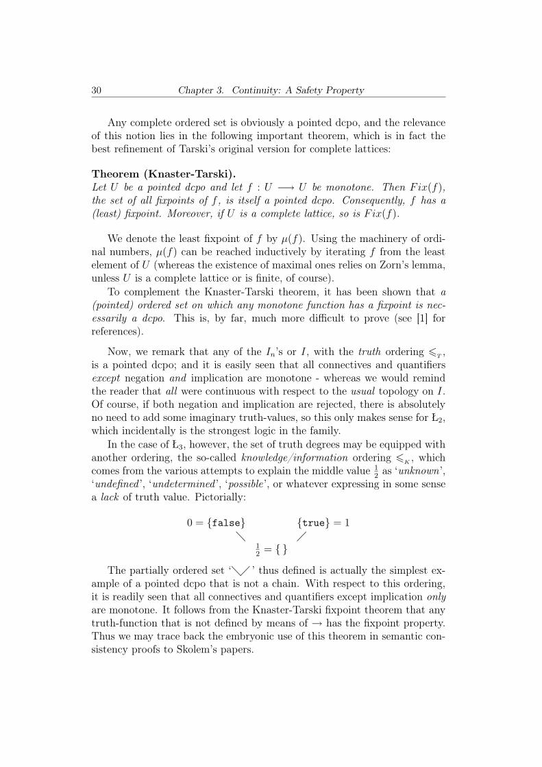
Now, we remark that any of the In’s or I, with the truth ordering �T ,is a pointed dcpo; and it is easily seen that all connectives and quantifiersexcept negation and implication are monotone - whereas we would remindthe reader that all were continuous with respect to the usual topology on I.Of course, if both negation and implication are rejected, there is absolutelyno need to add some imaginary truth-values, so this only makes sense for Ł2,which incidentally is the strongest logic in the family.

In the case of Ł3, however, the set of truth degrees may be equipped withanother ordering, the so-called knowledge/information ordering �K , whichcomes from the various attempts to explain the middle value 1

2 as ‘unknown’,‘undefined ’, ‘undetermined ’, ‘possible’, or whatever expressing in some sensea lack of truth value. Pictorially:

0 = {false} {true} = 1� �

12 = { }

The partially ordered set ‘�� ’ thus defined is actually the simplest ex-ample of a pointed dcpo that is not a chain. With respect to this ordering,it is readily seen that all connectives and quantifiers except implication only

are monotone. It follows from the Knaster-Tarski fixpoint theorem that anytruth-function that is not defined by means of → has the fixpoint property.Thus we may trace back the embryonic use of this theorem in semantic con-sistency proofs to Skolem’s papers.

3.10. Kripke-style models 31

3.10 Kripke-style modelsInterestingly it is again the same theorem that is implicitly invoked, but atanother level, in Gilmore and Brady’s work in providing their term models.

Roughly, the universe of these models is fixed in advance and made ofset abstracts, regarded as syntactical expressions of the form {x | ϕ} forsuitable formulas ϕ (e.g. Lτ

+∗ , Lτ

�→∗ ); and then, by a fixpoint argument, the

membership relation is determined inductively in such a way that {x | ϕ} bea solution to the ϕ-instance of the abstraction scheme under consideration.

This so-called inductive method was later popularized by Kripke [25] inhis work on the liar paradox. For a comprehensive description and analysisof the connection between these works, we may refer the reader to [14].

We will see the inductive method in action in Chapter 6 where we reviewand complete the results in [24].

Let us here sing the praises of another useful technique which has itssource in Scott’s seminal work on the λ-calculus. As anyway we will needsome basic facts about dcpo’s in this thesis, we first supply the reader witha few prerequisites, referring systematically to [1] for more complete treat-ments.

3.11 Addendum on dcpo’sDealing with dcpo’s, it is natural to be concerned with those monotone func-tions that preserve suprema of directed subsets. Let U, V be dcpo’s. We saythat a function f : U −→ V is Scott-continuous if and only if f is monotoneand for all directed subset D ⊆ U , we have f ‘ D = f“D. (Note thatScott-continuous functions need not preserve least elements when they ex-ist.) The relevance of this notion lies in the fact that, for a Scott-continuousfunction f on a pointed dcpo, ω steps (at most) are enough to reach µ(f).

We write �U → V � for the set of all Scott-continuous functions U −→ V .It is easy to see that �U → V �, equipped with the pointwise ordering, isitself a dcpo, and then that µ : �U → U� −→ U is Scott-continuous. We letDCPO stand for the category of dcpo’s with Scott-continuous functions asmorphisms, and we refer the reader to [1] for any property of DCPO we shallmention and use without proof. Notice in particular that it is shown in [1]that DCPO is cartesian closed, the exponential of which being just �·→ ·�.

The appropriate topology for a dcpo is called the Scott topology ; this iscoarser than the Alexandroff one. Given a dcpo U , we say that A ⊆ U isScott-open if and only if A is an upper set and for any directed set D ⊆ U ,

D ∈ A ⇒ D∩A �= ∅ ; and thus we say that B ⊆ U is Scott-closed if and only


if B is a lower set and for any directed set D ⊆ U , D ⊆ B ⇒ D ∈ B. It isnow easily seen that the Scott-topologically-continuous functions are exactlythe Scott-continuous ones as defined above. It is also apparent that A ⊆ U

is Scott-open if and only if ıU ‘A : U −→ 2 is Scott-continuous, where 2 isequipped with its natural truth ordering (i.e. 0 < 1). Likewise, one can seethat B ⊆ U is Scott-closed if and only if ıU ‘B : U −→ 2∗ is Scott-continuous,where 2∗ is the order dual of 2 (i.e. 1 < 0). Obviously 2 ∼= 2∗, but this willresult in some schizophrenia, as we shall see in Chapter 5 notably.

3.12 Scott-style models

In providing models for the untyped λ-calculus, Scott discovered that theKnaster-Tarski theorem is reflected within suitable subcategories of DCPO .

Roughly, it was proved that for a wide variety of functors F(·) acting onthose categories, the reflective equation U ∼= F(U) has a least solution (ob-tained by inverse limit). Such fixpoints have naturally proposed themselvesas semantic domains of programming languages, so the mathematical branchin theoretic computer science that investigates this is called domain theory.We again rely on [1] for proofs and further motivation.

Let T stand in what follows for I2 (= 2) with the truth ordering �T , orfor I3 with the knowledge ordering �K , both of which, we recall, are dcpo’s.

It is very tempting, by using techniques of domain theory, to try to solve areflexive equation of the form U ∼= F(U) ⊆ [U → T ], where this latter is theset of all monotone functions U −→ T (which is a dcpo as well). Any fixpointsolution U to such an equation will thus give rise to a set-theoretic universe inwhich sets are conceived of as some special but monotone functions U −→ T .Therefore, by virtue of the monotonicity of the connectives and quantifiers,and for a suitable choice of F(·), such a U may seem to be a good candidatefor an extensional normal model of Comp[L +] when T is �I2; �T �, or ofComp[L �→] when T is �I3; �T �.

However attractive this idea is, it will not enable us to recover equalityin formulas defining sets. This is because =U is not monotone on a normalstructure U . Let us illustrate this with the two-valued case. We may assumethat U is a pointed dcpo and that |U | > 1, so that there do exist distinct u, v

in U such that u �U v.7 Now, if =U : U × U −→ 2 was monotone, then weshould have =U ‘(u, u) �T =U ‘(u, v), which is impossible since =U ‘(u, u) = 1and =U ‘(u, v) = 0. A similar argument applies to the 3-valued case.

7 This follows from the fact that U is a solution in DCPO to U ∼= F(U) ⊆ [U → T ].

3.13. The solution 33

Equality is still missing, but the idea remains appealing in that it couldthen serve to provide natural models of Comp[L +

∗ ] or Comp[L �→∗ ].

Surprisingly it turns out that the least solution U to U ∼= �U → 2� is justone of the twin models of Comp[L +

∗ ] given by Skolem in [37, 38]. This isgoing to be proved in Chapter 5, where it is further shown that U is actuallya model of Abst� [Lτ

+∗ ] + Ext. The other twin model can be obtained as

the least solution to U ∼= �U → 2∗�. Of course, these are isomorphic asdcpo’s (because 2 ∼= 2∗), but not as set-theoretic structures (for the Scott-isomorphisms [·]U differ). As a matter of fact, topologically speaking, in theone the collectable subsets are just the Scott-open subsets, whereas in theother these are the Scott-closed ones, whereby we thus establish in Chapter5 the existence of topological models of positive abstraction.

Such an attempt for the 3-valued case is largely explored in [5], but withlittle success. Nevertheless, the authors finally show that the structure soconstructed contains a model of ‘rough set theory ’ within its maximal ele-ments (see also [6]). As we shall see in Section 4.7, this is another (verydifferent) example of topological model actually.

It should also be remarked that, curiously, the 3-valued paraconsistentapproach has proved more successful than the 3-valued paracomplete one. Wemay again refer the reader to [27] for a sketchy analysis of that asymmetry.

3.13 The solutionTopological considerations have thereby come on. And now we have someexamples of topological models U satisfying U ∼= Pop(U) /U ∼= Pcl(U), thequestion as to which of these, if any, may suit our purposes best is legitimate.

Clearly, if our goal is to recover identity in formulas defining sets, onlythose that are solution to U ∼= Pcl(U) are worth being sought after, but thenwithin categories of, at least, T1-spaces, which dcpo’s are not.

As any deep piece of work, Scott’s has been a source of inspiration. Thus,it was shown in [4] that another famous fixpoint theorem involving continuous

functions is also reflected within some suitable category. This theorem isBanach’s for contracting functions on complete metric spaces, cms for short,which too have been successfully used in modelling programming processes.8

Now, by using the technique described in [4], it is proved that the reflexiveequation U ∼= Pcl(U) has a unique (up to isomorphism) solution amongcms’s, which are T2-spaces. This solution is just the space Nω we mentioned

8 Recently, the framework of so-called ‘continuity spaces’, a common refinement of par-tially ordered sets and metric spaces, has been proposed to develop a general theory ofsemantics domains. The interested reader is referred to [16].


in Section 2.4, which, as said, turns out to be a model of Comp[L [+]] +Ext.The equality relation makes hereby its entrance in formulas defining setswithin an extensional universe; and as in Ł2 this entrance coincides with theone of =. , some bounded quantifications had anyhow to come along with. Itis then not surprising that Nω fulfils Comp[L [+]], and not only Comp[L +].Besides, as stressed in Section 2.3, L [+] is not an unnatural class of formulas.

We thus have related the emergence of a natural topological solution to‘the consistency problem for positive comprehension principles’, which, aswe saw, originated in the use of ‘deviant’ logics. Note that Nω is actuallythe simplest member of a family of topological solutions whose existence wasestablished in [17] (relying on some large cardinal assumptions, and withoutany reference to [4]). These structures, subsequently called hyperuniverses,have extensively been studied by Forti, Honsell and Lenisa in several papers,e.g. in [18], where the authors even proposed hyperuniverses as an universalframework for investigating the semantics of programming languages.

In such topological models the collectable subsets are just the closed ones.Thus, even though not every class can define a set, each class in such modelsmay, at least, be optimally approximated by the smallest set containing it.This alternative proposal was the core of Weydert’s thesis [40], in whichthe author was independently led to proving the existence of hyperuniverses.Note that the constructions given in [17] and [40] were actually both inspiredby the pioneer work of Malitz [30]; see [17] for an historical account.

Such an idea of approximation of the full comprehension scheme wasoriginally considered by Skala in [34], and then refined by Manakos in [31].9Although semantic proofs of the consistency of (some extensions of) Skala’stheory appeared in [33], [39] and [20], it seems that no topological attemptto characterize the models has been made. So in the next chapter we revisitSkala’s topological set theory on both the axiomatic and semantic sides.

9 Skala’s paper is cited in the references of [40], and even in those of [30], but with nofurther comment.

Chapter 4

ON TOPOLOGICAL SET THEORY

We review and resume the results in [34] & [31] so as to give new insightsinto them. In most cases the proof is just routine but is not omitted for allthat. Our most significant results are Theorem 4.5.4 - a negative one - andTheorem 4.6.5 - a rather positive one.1 Both follow from a straightforwardtopological characterization of the models of the theories considered in [34]& [31]. This seems not to have been noticed before. The content of thischapter is recapitulated in [13]. Note that Extensionality is tacitly assumedthroughout this chapter, and that a set-theoretic structure U is looked at as�U ; [·]U �. It is also worth remembering the abbreviations given in Section 2.1.

4.1 The closure schemeWe are interested here in any extensional set theory based upon the followingapproximation scheme:

(✸) :For every formula ϕ(x),∃y(∀x(ϕ → x ∈ y) ∧ ∀z(∀x(ϕ → x ∈ z) → y �. z)).

In words, (✸) asserts the existence for every formula ϕ(x) of a least setcontaining ‘{x | ϕ(x)}’. We denote this (unique) set by {x |✸ ϕ}.

If {x |✸ ϕ} = ‘{x | ϕ(x)}’, we shall say that ϕ is continuous w.r.t. x.Note that we will use that terminology in (✸)-free context as well, so thatϕ is continuous w.r.t. x simply means that ‘{x | ϕ(x)}’ is a set. A centralquestion is then to know which formulas can be continuous, and in a type-freesetting this may be split up into two parts, not independent of each other:which atomic formulas can be continuous, and which logical connectives canpreserve the continuity of a formula; these will be said to be continuous too.

Assuming (✸), x = x, p = p, and � are equally continuous w.r.t. x; theyall define the universal set V. Notice also that x ∈ p is clearly continuous

1 This latter in particular is due to Olivier Esser.

36 Chapter 4. On Topological Set Theory

w.r.t. x, seeing that {x |✸ x ∈ p} = p. The continuity of p = x w.r.t. x isequivalent to the axiom (A ), and the one of p ∈ x is (B). These are goingto be largely discussed. Finally, x ∈ x may be continuous w.r.t. x only if ¬is not continuous. And, of course, that ¬ preserves continuity is just (C ).

It is easy to see that ∧ and ∀ are continuous under (✸) once we notice thatthis latter is equivalent to the following scheme of definable intersections:

(∩δ) :For every formula ψ(z),∃y∀x(x ∈ y ↔ ∀z(ψ → x ∈ z)).

We denote this unique set y by ‘{z | ψ(z)}’.

Proposition 4.1.1. (✸) ⇔ (∩δ).

Proof.

⇒ : ‘{z | ψ(z)}’ = {x |✸ ∀z(ψ → x ∈ z)}.⇐ : {x |✸ ϕ} = ‘{z | ∀x(ϕ → x ∈ z)}’. �

Corollary 4.1.2. Under (✸), ∧ and ∀ preserve the continuity of a formula.

Proof. Assume (∩δ) and suppose that ϕ(x, y) is continuous w.r.t. x. From‘{x | ∀yϕ(x, y)}’ = ‘{z | ∃y(z = ‘{x | ϕ(x, y)}’)}’ it follows that ∀yϕ(x, y)is continuous w.r.t. x; and, obviously, that ∧ preserves continuity results inthe possibility of defining p ∩ q by ‘{z | z = p ∨ z = q}’. �

It is worth stressing that Proposition 4.1.1. shows that (✸) is just equiv-alent to particular instances of comprehension. Namely, Comp[ϕ(x)] whereϕ(x) is of the form ‘∀z(ψ → x ∈ z)’, for any L -formula ψ (with the provisothat x does not occur free in ψ).

By a closure operator on D ⊆ P(U) we mean a ⊆-preserving application(·)✸ : D −→ D such that A ⊆ A✸ and (A✸)✸ = A, for any A ∈ D.2 A subsetA of U is said to be closed if it lies in rng(·)✸, that is, if A✸ = A.

Given a structure U , we recall that def[·]U stands for the set of definable

subsets. What follows is an elementary characterization of the models of (✸).

Theorem 4.1.3. A set-theoretic structure U is a model of (✸) if and only if

there exists a closure operator (·)✸ on def[·]U such that rng[·]U = rng(·)✸.

Proof. �x | ϕ(x, v)�✸U

= [{x |✸ ϕ}U(v)]U for any formula ϕ(x, p) and v in U . �

2 When D = P(U), we usually say a closure operator on U .

4.2. Duality 37

This simple observation will enable us to easily answer natural questionson some extensions of (✸) we are going to consider. Still more useful forconstructing models is the second-order formulation of Theorem 4.1.3, inwhich (·)✸ is now a closure operator on U and (✸) is replaced by ((✸)).3

In all the examples we consider, it is even the case that (·)✸ is the closureoperator associated with some (maybe trivial) topology on U , i.e. (·)✸ furthersatisfies ∅✸ = ∅ and (A ∪ B)✸ = A

✸ ∪ B✸, for any A,B ⊆ U . This is, of

course, what has motivated the title of this chapter. Notice that in suchcircumstances, Λ exists and ∨ is continuous too. It thus remains to explore(A ), (B), (C ) and the continuity of ∃ under (✸).

Remark 4.1.1. The second-order version of Proposition 4.1.1 is the translationof the well-known correspondence between closure operators and (topped) in-tersection structures, which are complete lattices. Then, given a set-theoreticstructure U , what follows is immediate.

Fact 4.1.1. If U |= ((∩δ)), then �U ; �. U� is a complete lattice.

Proof. We observe that, for any A ⊆ U , A := ( ‘{z | z ∈ A}’)U is theinfimum of A in �U ; �. U�. �

We would just notify the reader that the converse of this does not hold.The spine model(s) described in Chapter 5 will provide us with an illumi-nating example. All we are able to say when �U ; �. U� is a complete lattice isthat, for any A ⊆ U , U |= ∀x(x ∈ A → ∀z(z ∈ A → z ∈ x)).

4.2 DualityThe previous considerations naturally prompt us to examine the symmetric

approach, according to which each class can be approximated from below.There is a priori no reason to prefer one view to the other. Besides, bothviews might equally well be taken simultaneously, which is going to be ex-amined in the next sections.

The dual version of the approximation scheme (✸) is defined as follows

(✷) :For every formula ϕ(x),∃y(∀x(x ∈ y → ϕ) ∧ ∀z(∀x(x ∈ z → ϕ) → z �. y))

and the unique y given by (✷) is designated by {x |✷ ϕ}.3 In the sequel, whenever we look at the second-order version of an axiom scheme, it

will be designated with double parentheses ‘(( ))’.


The scheme of definable intersections is now to be replaced by the one ofdefinable unions :

(∪δ) :For every formula ψ(z),∃y∀x(x ∈ y ↔ ∃z(ψ ∧ x ∈ z))

and we denote this y by ‘{z | ψ(z)}’.

Proposition 4.2.1. (✷) ⇔ (∪δ).

Proof.

⇒ : ‘{z | ψ(z)}’ = {x |✷ ∃z(ψ ∧ x ∈ z)}.⇐ : {x |✷ ϕ} = ‘{z | ∀x(x ∈ z → ϕ)}’. �

Corollary 4.2.2. Under (✷), ∨ and ∃ preserve the continuity of a formula.

In the same way, one could give a characterization of the models of (✷)in terms of interior operators. We would leave this to the reader.

Naturally, from the semantic point of view, this duality just consists intaking the complement: we define the dual Uc of a set-theoretic structure Uto be �U ; U × U \∈U�, so that U |= (✸) / (✷) if and only if Uc |= (✷) / (✸).

Assuming (C ), the duality is still more obvious on the axiomatic side.

Proposition 4.2.3. (✸) + (C ) ⇔ (✷) + (C )

Proof. {x |✷ ϕ} = C ({x |✸ ¬ϕ}) and likewise by interchanging ✸ and ✷. �

Surprisingly enough, if one is considering (A ), the symmetry is broken:

Fact 4.2.1. (✷) ⇒ non(A ), whereas (✸) + (A ) is consistent.

Proof. Using (∪δ), we define r := ‘{z | ∃w(z = A (w) ∧ w /∈ w)}’. Clearly,we have r ∈ r → r /∈ r, and if A (r) existed, we would too have r /∈ r → r ∈ r.For the consistency of (✸) + (A ), we rely on the existence of Nω. �

Despite the loss of singletons, we are going to be interested in any possibleset theory based upon both (✸) and (✷). This was initiated in [34], where (C )is taken too, and then reinvestigated in [31] without assuming (C ) anymore.

4.3. The comprehension scheme revisited 39

4.3 The comprehension scheme revisitedBy taking (✷), we must give up (A ). Nevertheless, we may use (✸) to definewhat we call pseudo-singletons or molecules (as named in [31]). By definition,the pseudo-singleton of p is the smallest set containing the singleton of p, thatis, {x |✸ p = x} = B(p), and this is nothing but M (p).

Proposition 4.3.1. (✸) + (✷) ⇔ (M ) + (✷).

Proof.

⇒ : Obvious.⇐ : For any formula ϕ(x), {x |✸ ϕ} = ‘{z | ∃w(z = M (w) ∧ ϕ(w))}’. �

The right to left part of the proof is interesting in that it shows that{x |✸ ϕ} = ‘{x | ∃w(w � x ∧ ϕ(w))}’, which leads to defining the scheme

(�) :For every formula ϕ(x),∃y∀x(x ∈ y ↔ ∃w(w � x ∧ ϕ(w)))

and then proving that

Proposition 4.3.2. (�) ⇔ (✸) + (✷).

Proof.

⇐ : y = {x |✸ ϕ}⇒ : If ϕ(x) is taken to be ∃z(x ∈ z ∧ψ(z)) in (�), what we get is just (∪δ).And if ϕ(x) is taken to be x = p , we have (M ). �

The axiom scheme (�) should not leave the reader indifferent, for if �was the equality - which is the case when (A ) holds (cf. Fact 2.1.1) - itwould be nothing but the full comprehension scheme. But that one wouldbe willing to sacrifice (A ) just because (�) is provably consistent wouldhardly be arguable in view of what follows.

Given a preorder R on a set U , we denote by (·)R the closure operatoron U that is defined by A

R := R“A ; and then, for any D ⊆ P(U), we letD↑ stand for {AR | A ∈ D} and D

↓ for {AR−1 | A ∈ D}.Given a set-theoretic structure U , �U is a preorder on U , and as it is

definable, we have def[·]↑U⊆ def[·]U and def[·]↓

U⊆ def[·]U , so that (·)�U is in

particular a closure operator on def[·]U .We are ready to formulate the semantic counterpart of Proposition 4.3.2.

Theorem 4.3.3. A model U of (✸) is a model of (✷) if and only if the

closure operator (·)✸given by Theorem 4.1.3 coincides with (·)�U , and thus

rng[·]U = def[·]↑U.


Proof. Assuming (✸), we have seen that {x |✸ ϕ} = ‘{x | ∃w(w � x ∧ ϕ(w))}’if and only if (✷) holds. �

Note that in any case, if (·)✸ was of the form (·)R for some preorder R onU , this should be �U :

Proof. Suppose u �U v. As {u}R is closed, there exists w ∈ U such that[w]U = {u}R, and then, as u ∈ {u}R, that is, u∈U w, we get v ∈U w, thatis, v ∈ {u}R. Whence u R v. Conversely, suppose u R v and let w ∈ U

such that u∈U w, that is, u ∈ [w]U . Now, as u R v and [w]U is closed, i.e.R“[w]U = [w]U , we have v ∈ [w]U too, that is, v ∈U w. Therefore u �U v. �

We thus may state the second-order version of Theorem 4.3.3 as follows

Theorem 4.3.4. A set-theoretic structure U is a model of ((�)) if and only

if there exists a preorder R on U such that rng[·]U = P(U)↑. In that case, R

must coincide with �U .

With this, it is rather child’s play to concoct models of ((�)), and inparticular finite ones, which would testify of the insignificance of (�) as aset theory on its own. Incidentally, there was no need to invoke Theorem4.3.4 to prove its consistency, as ‘{Λ, V}’ is obviously the simplest model,and this is also a model for the situation we examine hereafter.

4.4 The symmetric caseWithout further assumptions, all the properties that � is certain to possessare reflexivity and transitivity. According to Fact 2.1.1, when (A ) fails,� may be thought of as a reminiscence of the equality. Then it would belegitimate to require the symmetry of �. Under (�), this actually amountsto demanding that the negation preserves the continuity of a formula.

Proposition 4.4.1.

i) (C ) ⇒ (x � y → y � x).

ii) Assuming (�), (x � y → y � x) ⇒ (C ).

Proof.

i) Suppose x � y. If x /∈ z, then x ∈ C (z), and so y ∈ C (z), that is, y /∈ z.ii) Suppose that (x � y → y � x). We show that {x |✸ x /∈ p} = C (p).Let x ∈ {x |✸ x /∈ p}. By (�), there exists w such that w � x and w /∈ p.Then x � w and it follows that x /∈ p either, that is, x ∈ C (p). �

4.4. The symmetric case 41

To sum up, a model U of (�) satisfies (C ) if and only if �U is an equiva-lence relation, namely .=U . Thence we can give the next useful characteriza-tion which falls out of Theorem 4.3.4.

Theorem 4.4.2. A set-theoretic structure U is a model of ((�))+(C ) if and

only if there exists an equivalence relation R on U together with a bijection

f : U −→ P(U/R) such that [u]U = f ‘u for each u ∈ U . In that case, R

must coincide with.=U .

Proof. Observe that (·)R-closed subsets are just unions of equivalences classes,and thus we have to have f ‘u := {{v}R | v ∈ [u]U}, for any u ∈ U . �

The simplified version that follows speaks for itself:

Theorem 4.4.3. A set U is the universe of a model of ((�)) + (C ) if and

only if |U | = 2κ, for some cardinal κ.

Proof.

Necessity: Follows directly from Theorem 4.4.2.Sufficiency: Take any equivalence relation R on U such that |U/R| = κ, andthen any bijection f : U −→ P(U/R) to define [·]U as in Theorem 4.4.2. �

At least, in assuming (�)+(C ), all the basic logical connectives (¬,∧,∨, ∀,∃) are continuous, but this results in serious drawbacks at the atomic level.We already know that (A ) is incompatible with (�). It turns out that (B) isalso incompatible with (�)+(C ), and this can happen in a (�)-free context:

Fact 4.4.1. If ¬, ∧, ∃ are continuous, then (B) is inconsistent.

Proof. Under the assumptions, x � y ≡ ¬∃z(x ∈ z ∧ y /∈ z) is continuousw.r.t. x, and then, if we assume that y ∈ x is continuous w.r.t. x, so is∃y(x � y ∧ y /∈ x). Now, let r be the set defined by this formula. It is easyto see that r ∈ r if and only if r /∈ r. �

Note that if the use of quantifiers is forbidden, this is no longer provable:

Fact 4.4.2. (B) is compatible with the use of ¬ and ∧ in formulas defining

sets.

A proof of this can be found in Skolem’s paper [38] (Theorem 2, p. 165).

Thus (A ), (B), and obviously (W) are all incompatible with (�) + (C ).Note incidentally that we are going to show in the next section that, as for(A ), (B) is already incompatible with (�) alone (this is not immediate).

To conclude and summarize, the next result - which is not mentioned in[34] or [31] - clearly states what the continuous formulas are under (�)+(C ).


Theorem 4.4.4. (�) + (C ) ⇔ Comp[ϕ(x)] for any formula ϕ(x) in L∗with the sole restriction that the abstracted variable x does not occur on the

right-hand side of ∈.

Proof.

⇒ : Follows from the continuity of all the logical connectives under (�) +(C ), and the fact that the limitation to L∗-formulas and the restriction onx prevent occurrences of p = x, p ∈ x, x ∈ x at the atomic level.⇐ : Observe that ‘{z | ψ(z)}’ = ‘{x | ∀z(ψ → x ∈ z}’ is just defined bysuch a suitable formula (note that as we assume extensionality, ψ can bereduced to an L∗-formula by replacing any occurrence of = by =. ). Thus weget ( δ). And that we have (C ) is still more obvious. �

It should be stressed that, as well as the absence of =, this simple restric-tion on the abstracted variable has disastrous effects on the development ofset theory, as for instance it prevents us from defining the power-set of anygiven set p , seeing that P(p) = ‘{x | ∀z(z ∈ x → z ∈ p)}’.

4.5 The antisymmetric caseThe absence of (C ) seems to leave the door open to the continuity of x ∈ x

and p ∈ x w.r.t. x. In fact, that (W) is compatible with (�) is easily seen:Example 4.5.1. Take U := {a, b, c} with R := U × U \{(b, a), (c, a)}, i.e.{a}R = {a, b, c}, {b}R = {b, c} = {c}R (so R is neither symmetric nor an-tisymmetric), and define [·]U as follows: [a]U := ∅, [b]U := {b, c}, [c]U := U .Thus, U is a model of ((�)) in which a is Λ, b is W, and c is V. Notice thatboth B(b) and B(c) exist and are equal to b, but B(a) does not exist in U .

Trying to find a model of (B) is directly a less obvious task for there isno finite model of (B) (see Chapter 5). Under (�), the task will soon provevain. To proceed, we first point out the following result (to be comparedwith Proposition 4.4.1).

Proposition 4.5.1.

i) (B) ⇒ (x � y → x �. y).

ii) Assuming (�), (x � y → x �. y) ⇒ (B).

Proof.

i) Suppose x � y. If z ∈ x, then x ∈ B(z), and so y ∈ B(z), that is, z ∈ y.ii) Suppose that (x � y → y �. x). We show that {x |✸ p ∈ x} = B(p).Let x ∈ {x |✸ p ∈ x}. By (�), there exists w such that w � x and p ∈ w.Then w �. x and it follows that p ∈ x too, that is, x ∈ B(p). �

4.5. The antisymmetric case 43

We are going to show that (x � y → x �. y) is incompatible with (�).In order to achieve this, we need a couple of lemmas.

Given a set-theoretic structure U , we say that a function f : U −→ P(U)is definable if there exists an L -formula ϕ(x, y, p) and v ∈ U such that forall u ∈ U , f ‘u = �x | ϕ(x, u, v)�U .

Lemma 4.5.2. Let U be a set-theoretic structure. If there exists a surjective

definable function f : U −→ def[·]↑U

such that u �U v ⇒ f ‘u ⊆ f ‘v, then there

exists such a surjective definable function g : U −→ def[·]↓U

Proof. We define g‘u for any u ∈ U by U \ {f ‘w | w /∈ f ‘u}, that is, for allx in U , x ∈ g‘u ⇔ ∀w ∈ U (x ∈ f ‘w → w ∈ f ‘u). Therefrom it is easy tosee that g : U −→ def[·]↓

Uis definable and satisfies u �U v ⇒ g‘u ⊆ g‘v. It

remains to show that g is surjective. Take A ∈ def[·]↓U. Clearly, U \A ∈ def[·]↑

Uand so, as f is surjective, we can choose b ∈ U such that f ‘b = U \A. SetB := {b}�U . As B ∈ def[·]↓

U, we have U \B ∈ def[·]↑

U, and so, again, we

can choose a ∈ U such that f ‘a = U \B. Now, we do have g‘a = A, for{f ‘w | w /∈ f ‘a} = {f ‘w | w ∈ B} = {f ‘w | w �U b} = f ‘b = U \A. �

Lemma 4.5.3. Given a set-theoretic structure U , there is no surjective de-

finable function g : U −→ def[·]↓U

such that u �U v ⇒ g‘u ⊆ g‘v.

Proof. Let g be as above. Define R = {u ∈ U | u /∈ g‘u}�U . Clearly,R ∈ def[·]↓

Uand so there exists r ∈ U such that g‘r = R. If we had r /∈ R, we

would too have r ∈ R by definition of R. Whence r ∈ R. But then there existsu0 ∈ U such that u0 /∈ g‘u0 and r �U u0. From this latter we get g‘r ⊆ g‘u0,and thus, as u0 ∈ R = g‘r, we have u0 ∈ g‘u0 as well. Contradiction. �

Theorem 4.5.4. (x � y → x �. y) - and so (B) - is incompatible with (�)

Proof. For suppose there exists U which is a model of (�)+(x � y ⇒ x �. y).Then [·]U would be a surjective (definable) function U −→ def[·]↑

Usuch that

u �U v ⇒ [u]U ⊆ [v]U , which is impossible in view of Lemmas 4.5.2–3. �

It does not seem possible to find a syntactical proof of Theorem 4.5.4.Such a proof, however, can be given for a slight variant of it.

Proposition 4.5.5. (x � y → y �. x) is incompatible with (�)

Proof. Let r be {x |✸ x /∈ x}, which, by (�), is ‘{x | ∃w(w � x ∧ w /∈ w)}’.Clearly r /∈ r → r ∈ r, so we must have r ∈ r. Then there exists w suchthat w � r and w /∈ w. If we assumed (x � y ⇒ y �. x), it would result thatw /∈ r, which is impossible for w ∈ r (since w /∈ w). �


We mention that the converse of (x � y → x �. y) is obviously consistentwith (�), as it holds in the two-points models ‘{Λ, V}’ or even in the modelgiven in Example 4.5.1. But this is a rather odd principle, as, for instance,it is apparent that ‘{Λ}’ cannot exist under (x �. y → x � y), which wouldnot really speak for any set theory in which this latter holds. Nevertheless,here is an example about which we should not be indifferent.

Proposition 4.5.6. Abst[Lτ+∗ ] + Ext ⇒ (x �. y → x � y).

Proof. Assume Abst[Lτ+∗ ] and let p, q be such that p �. q but p �� q. De-

fine σ(x) := {z | z ∈ p ∨ (x ∈ x ∧ z ∈ q)}. It easily follows from p �. q that∀x((x ∈ x → σ(x) = q)∧(x /∈ x → σ(x) = p)) (Ext is needed for this). Now,as p �� q, let us choose r with p ∈ r, q /∈ r, and define ρ = {x | σ(x) ∈ r}.Thus we have ∀x(x ∈ ρ ↔ x /∈ x), and therefore ρ ∈ ρ ↔ ρ /∈ ρ. �

Although we have assumed Ext throughout this chapter, it was importantto mention its use in Proposition 4.5.6, for otherwise one might have beentempted to think that Abst[Lτ

+∗ ] ⇒ (x =. y → x

.= y), which is false. As weshall see in Chapter 6, there are term models for Abst[Lτ

+∗ ] in which �

Ext

fails, as well as there are in which it holds, and the proof of this is particularlynot obvious. The consistency of Abst[Lτ

+∗ ] + Ext will fall out more easily

of Chapter 5 in which we show that Abst[Lτ+∗ ] - and so (B) - is at least

compatible with (✸) and (✷) separately.

In assuming (B) (and Ext), � is anti-symmetric, i.e. (x .= y → x = y).It is then legitimate to enquire whether this natural principle could not becompatible with (�). At least, it would prevent the existence of finite models.

Fact 4.5.1. Any model U of (Λ) + (M ) + (x .= y → x = y) is infinite.

Proof. Notice that x.= y ⇔ M (x) = M (y) and that Λ = M (x) for no x.

Then it is clear that, under the assumptions, we can define a potentiallyinfinite sequence of elements in U by iterating M (·) from ΛU . �

The consistency of (�) + (x .= y → x = y) is raised and left open in [31].By invoking Theorem 4.3.4, it is now fairly easy to give a positive answer.

Example 4.5.2. Take U := , R the usual ordering � on , and define [·]Uas follows: [0]U := ∅, [n]U := {m | n−1 � m}, for any n � 1. Thus it is clearthat rng[·]U is just the collection of (·)R-closed subsets of U , so U |= ((�)).In U , 0 is Λ, 1 is V, and 2 is W, which shows that this latter can exist when� is antisymmetric. On the other hand, note that B(u) exists for no u in U .

4.6. Normality 45

4.6 NormalityAssuming (✷), not every singleton can exist, so we shall say that a set x

is normal if ‘{x}’ exists. No surprises, as we show in this section, very fewthings can be said about the class of normal sets, which is defined by

N := ‘{x | ∃y(y = A (x))}’ .

Proposition 4.6.1. ∃x(x /∈ N ).

Proof. Just a reformulation of the first part of Fact 4.2.1. �

On the other hand, ∃x(x ∈ N ) is not even derivable from (�) + (C ),for in the two-points model ‘{Λ, V}’ we have N = Λ. As certified by thisexample, it can be shown, at least, that N is always a set.

Lemma 4.6.2. For any formula ϕ(x), if z ∈ N and ϕ(z), then z ∈ {x |✷ ϕ}.

Proof. Suppose ϕ(z) and z ∈ N . Then, {x |✷ ϕ}∪A (z) is a set, and as wehave ∀x(x ∈ {x |✷ ϕ}∪A (z) → ϕ), it follows that {x |✷ ϕ}∪A (z) �. {x |✷ ϕ}.Whence z ∈ {x |✷ ϕ}. �

Proposition 4.6.3. N is a set.

Proof. Take ϕ(x) to be ∃y(y = A (x)) in the previous lemma. �

Such a simple question as to know whether N ∈ N or not is undecidable.In the two-points model, we have N = Λ, so that N /∈ N is consistent;and by invoking Theorem 4.4.2, it is easy to concoct a model U of (�)+ (C )in which, for instance, N = A (N ), so that N ∈ N is also consistent.

Example 4.6.1. Take U = {a, b, c, d}, with {d} and {a, b, c} as R-classes, andwith [a]U := ∅, [b]U := {a, b, c}, [c]U := U, [d]U := {d}. In U , d is N .

With the help of Lemma 4.6.2, we can also give an eloquent characteriza-tion of abnormal sets. These are just tokens of the discontinuity of a formula,in the following sense:

Proposition 4.6.4. z /∈ N if and only if there exists a formula ϕ(x) such

that ϕ(z) but z /∈ {x |✷ ϕ}.

Proof.

Necessity: Just take ϕ(x) to be z = x.Sufficiency: Use Lemma 4.6.2. �


Perhaps the most significant manifestation of the absence of control overN is the following seemingly positive result, which states that N may betaken to be any preexisting universe of normal sets (e.g. a model of ZF ).

Theorem 4.6.5. Let V be any infinite extensional set-theoretic structure

satisfying (A ). Then there exists a model U of ((�)) + (C ) such that:

(i) [·]V = [·]U restricted on V ;

(ii) V = {u ∈ U | U |= u ∈ N } ;

(iii) P(V ) ⊆ rng[·]U .

Proof. Let U be V ∪ V� ∪ V

��, where V� := P(V )\ rng[·]V and V

�� is anyset of cardinality 2|V |, and where we also assume that V, V

�, V

�� are pairwisedisjoint. We now equip each of these with an equivalence relation: we defineS on V by V/S := {{v} | v ∈ V }, S

� on V� by V

�/S� := {V �}, and we take any

equivalence S�� on V

�� such that |V ��/S��| = |V | and |K| � 2, for all K ∈ V

��/S�� .

Then we let R stand for the equivalence on U defined by S ∪S� ∪S

��. Noticethat |U | = |P(U/R)| = 2|V |. Thus, if we set f ‘v := {{w} | w∈V v} for eachv ∈ V and f ‘W := {{w} | w ∈ W} for all W ∈ V �, then f can be so extendedover U as to define a bijection U −→ P(U/R). By invoking Theorem 4.4.2,we can now turn U into a set-theoretic structure U |= ((�)) + (C ) by setting[u]U := f ‘u for any u ∈ U . It remains to check that U satisfies (i), (ii), (iii).For any v ∈ V , we have [v]U = {{w} | w∈V v} = {w | w∈V v}, and this isjust [v]V . In particular, since V |= (A ), we have {v} = [A V(v)]V = [A V(v)]U ,which shows that U |= v ∈ N and that A U(v) = A V(v), for any v ∈ V .Conversely, suppose U |= u ∈ N , that is, {u} = A for some A ⊆ U/R. Ifwe had A ∩ (V �

/S� ∪ V��/S��) �= ∅, we would have | A| � 2, for V

� is infiniteand |K| � 2 for any K ∈ V

��/S�� . Therefore we must have A ⊆ V/S, and so

{u} ⊆ V . Finally, let W ⊆ P(V ). If W ∈ rng[·]V , then clearly W ∈ rng[·]U .If W /∈ rng[·]V , W ∈ V �, and then [W ]U = f ‘W = W , so W ∈ rng[·]U . �

Has the scheme (�) + (C ) been to some extent salvaged by this result?In view of the arbitrary nature of the model constructed in the proof, itseems not. A possible way to try to define a notion of coherence in models of(�) + (C ) is discussed in the next and last section, in which we summarizethe mathematical content of this chapter.

4.7 CoherenceGiven a topological space U , we recall that Pcl(U) stand for the set of closed

subsets of U , and Pop(U) for the set of open ones.

4.7. Coherence 47

Clearly, according to the second-order version of Theorem 4.1.3 / its dual,any topological space U such that U � Pcl(U) /U � Pop(U) gives rise toa model of ((✸))/((✷)). Notice that the closure/interior operator attachedto a given model of ((✸))/((✷)) need not be topological. For our purposes,however, we shall restrict ourselves to topological models. But even in thatcase there are still many insignificant models of ((✸))/((✷)), in particularfinite ones. So in what remains of this chapter we shall rather be concernedwith topological models that are solutions to U ∼= Pcl(U) /U ∼= Pop(U)within specific categories of topological spaces. Anyhow, as we aim to show,the existence of such solutions is closely related to the consistency problem ofsome natural extensions of ((✸))/((✷)). It may also be said that such solutionsU to U ∼= Pcl(U) /U ∼= Pop(U) define natural models for ((✸))/((✷)), in thatthe extension function [·]U is to be not only a bijection but a homeomorphism,which does guarantee that there is some coherence in the process of assigningextensions to sets. It is understood here that Pcl(U) /Pop(U) has itself beenequipped with a natural topological structure derived from the one of U .

Alexandroff spaces

Any model of ((�)) is topological. This is a direct consequence of Theorem4.3.4 which states that such a model appears as a preordered set �U ; R�such that U � P(U)↑; and this latter is just Pop(U) when U is endowedwith the Alexandroff topology. Notice that, as P(U)↑ = P(U∗)↓ whereU∗ is �U ; R−1�, any model of ((�)) may equally be viewed as a topological

solution to U � Pcl(U), where U is now endowed with the Alexandrofftopology of U

∗. This is what is implicit in Theorem 4.3.4, for (·)R is aclosure operator, not an interior one. Still, it is more natural to view P(U)↑

as Pop(U). The reason why is that then R - and so �U - coincides withthe so-called specialization preorder ✁U of the topology, which is definedby u ✁U v ⇔ ∀A ∈ Pop(U)(u ∈ A → v ∈ A). This is also referred toas the indiscernibility relation associated with the topology, for u �U v ⇔∃A ∈ Pop(U)(u ∈ A∧ v /∈ A) ⇔ ‘u is discernible from v’, in topological terms.

It is clear that for any topological space U we have Pop(U) ⊆ P(U)↑,where this latter is taken with respect to ✁U ; and then it is easy to see thata topological space U will satisfy Pop(U) = P(U)↑ if and only if Pop(U)is closed under taking arbitrary intersections, that is to say, if this latteralso defines the set of closed subsets for some topology on U . We call thosetopological spaces Alexandroff spaces. Their topology is thus generated by apreorder, which must coincides with the specialization preorder.

All that to say that a model of ((�)) is just a solution U to U � Pop(U)within ALEX , the category of Alexandroff spaces. The Alexandroff-continuous


functions are the functions that preserve the indiscernibility relation.Given an Alexandroff space U , a possible way to transfer the indiscerni-

bility relation onto P(U), and thus to turn this latter into an Alexandroffspace, is by defining A ✁P(U) B if and only if A ⊆ B

✁U . The restrictionof this to Pop(U) = P(U)↑ is just the inclusion relation ⊆. In words, A isdiscernible from B in Pop(U) if and only if there exists a ∈ A with a /∈ B.

We now remark that, with that topology on Pop(U), the equation U ∼=Pop(U) is unsolvable within ALEX . The syntactical first-order translation ofthis ‘Cantor’s theorem’ for ALEX is just the incompatibility of (B) with (�)(cf. Theorem 4.5.4). Yet, the situation is by far less disastrous in ALEX thanin SET , for there are some (infinite) U here such that |Pop(U) \ rng[·]U | = 1.This will be illustrated in Chapter 5 where we exhibit a solution to U ∼=Pop(U) within SCOTT , the category of Scott spaces, which are just the dcpo’sendowed with the Scott-topology. Notice that the specialization preorder ofa Scott-space coincides with the ordering of the corresponding dcpo.Remark 4.7.1. Another possible way to make P(U) into a Alexandroff spaceis by defining A ✁P(U) B if and only if B ⊆ A

✁U , which may even seemmore natural for then U −→ P(U) : u �−→ {u} is Alexandroff-continuous.The restriction of this to Pop(U) is now the reverse inclusion ⊇, and thatU ∼= Pop(U) is still unsolvable within ALEX follows from Proposition 4.5.5.Likewise, one can show that the equation U ∼= Pcl(U), whether this latteris equipped with ⊆ or ⊇, is unsolvable within ALEX . Incidentally, a proofof this in the case where Pcl(U) is equipped with ⊆ was originally given in[11], where it was shown that, given an ordered set U , there is no surjectivemonotone function U −→ P(U)↓ (a second-order version of Lemma 4.5.3).

Quasi-discrete spaces

If the specialization preorder of an Alexandroff space is symmetric, that isto say, is an equivalence relation, we say that U is a quasi-discrete space.It is very easy to see that a topological space U is quasi-discrete if andonly if Pop(U) = Pcl(U). In words, the topology of a quasi-discrete spaceis generated by an equivalence relation: the open subsets, as well as theclosed ones, are just unions of equivalence classes. We call the category ofquasi-discrete spaces QUASI (this is a sub-category of ALEX ). Accordingto Theorem 4.4.2, a model of ((�)) + (C ) is just a solution U to U � Pop(U)- equally U � Pcl(U) - within QUASI ; in such a U .=U coincides with ✁U .

Now, given a quasi-discrete space U , the appropriate way to enrol P(U)in QUASI is by defining A ✁P(U) B if and only if A ⊆ B✁U and B ⊆ A✁U ,i.e., if and only if A

✁U = B✁U , which is thus an equivalence relation on P(U).

But the restriction of this to Pop(U)/Pcl(U) is the identity, so that, for more

4.7. Coherence 49

obvious reasons here, there is no solution U to U ∼= Pop(U)/U ∼= Pcl(U)within QUASI , for such a U would be a model of (�)+(C )+(x .= y → x = y).Remark 4.7.2. Referring back to Remark 2.3.1, it is easily seen that for aset-theoretic structure U in QUASI , demanding that [·]U : U −→ P(U) becontinuous actually amounts to demanding that ✁U is a bisimulation.

Nevertheless, it is possible to define a consistent notion of coherence inmodels of ((�)) + (C ). We shall say that a solution U to U � Pop(U)within QUASI is acceptable if for any indiscernible u, v in U , that is, withu ✁U v, either [u]U = [v]U = ∅ or [u]U ∩ [v]U �= ∅, which clearly vouchesfor a certain coherence in the process of assigning extensions to sets. Thefirst-order translation of this condition on the axiomatic side is expressed by(x .= y → x � y), where x � y :≡ ((x = Λ ∧ y = Λ) ∨ ∃z(z ∈ x ∧ z ∈ y)).

At least, any acceptable solution is infinite, as the next observation shows:

Fact 4.7.1. Any model U of (Λ) + (M ) + (C ) + (x .= y → x � y) is infinite.

Proof. First notice that Λ � M (x) for no x, and that, as � coincides with.= under (C ), we have M (x) � M (y) ⇒ x

.= y. Then it follows from theassumptions that we can define a potentially infinite sequence of elements inU by iterating M (·) from ΛU (as in Fact 4.5.1). �

Just to stress the combinatoric nature of seeking an acceptable solution,we now formulate the corresponding version of Theorem 4.4.2.

Fact 4.7.2. A set U is the universe of an acceptable solution if and only ifthere is an equivalence R on U together with a bijection f : U −→ P(U/R)such that u R v ⇒ f ‘u ∩ f ‘v �= ∅ or f ‘u = f ‘v = ∅.

Interestingly, the existence of an acceptable solution was established in[5], without any reference to Skala’s set theory. The authors used that struc-ture to promote what is called ‘rough set theory ’ (see also [6]). As furtivelymentioned in 3.12, that solution, whose cardinality is 22ℵ0 , arises from aninverse limit construction in DCPO . Although we admit to not having madeany serious attempt, it might be interesting to try to characterize those µ

such that 2µ is the cardinal of the universe of an acceptable solution. Callsuch a cardinal acceptable. If the construction given in [5] generalizes to κ-dcpo’s for any regular cardinal κ - which seems to be the case - then 2κ isacceptable. But perhaps there is a more direct way to generate acceptablesolutions; and then, can one prove an acceptable version of Theorem 4.6.5?

Chapter 5

SKOLEM’S SPINE MODEL(S)

The twin models we present here first appeared in [37], and then in [38]where Skolem finally proved the consistency of Comp[L +

∗ ]. We show inthis chapter that these are in fact natural topological models of Abst� [Lτ

+∗ ],

(re)establishing by the way the consistency of Abst[Lτ+∗ ]+Ext (see [26]). We

then start the comparison between (✸) + Abst[Lτ+∗ ] and (✸) + Comp[L [+]].

5.1 The B-sequenceAny model of Comp[L +

∗ ] is a model of (Λ) + (V) + (W) + (B), so we startby looking - as Skolem did - at sets which arise from Λ & V under (B).

Assume (B) and define inductively Bn(v), for n ∈ , as follows:

B0(v) := v

Bn+1(v) := B(Bn(v)).

It is then easily checked that, for each n ∈ ,

∀x∀y(Bn(x) ∈ Bn(y) ↔ x ∈ y) (†).

Now, let Λn := Bn(Λ) and Vn := Bn(V), for any n ∈ .

Proposition 5.1.1. Assuming (Λ) + (V) + (W) + (B), we have

(1) for any m,n ∈ , Λm /∈ Λn and Vm ∈ Vn ;

(2) for any m,n ∈ , m < n ⇔ Λm /∈ Vn ⇔ Vm ∈ Λn ;

(3) for any n ∈ , Λn /∈ W and Vn ∈ W ;

(4) for any n ∈ , W /∈ Λn and W ∈ Vn .

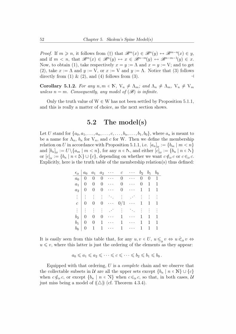
52 Chapter 5. Skolem’s Spine Model(s)

Proof. If m � n, it follows from (†) that Bm(x) ∈ Bn(y) ↔ Bm−n(x) ∈ y,and if m < n, that Bm(x) ∈ Bn(y) ↔ x ∈ Bn−m(y) ↔ Bn−m−1(y) ∈ x.Now, to obtain (1), take respectively x = y := Λ and x = y := V; and to get(2), take x := Λ and y := V, or x := V and y := Λ. Notice that (3) followsdirectly from (1) & (2), and (4) follows from (3). �

Corollary 5.1.2. For any n, m ∈ , Vn � .= Λm; and Λn � .= Λm, Vn � .= Vm

unless n = m. Consequently, any model of (B) is infinite.

Only the truth value of W ∈ W has not been settled by Proposition 5.1.1,and this is really a matter of choice, as the next section shows.

5.2 The model(s)Let U stand for {a0, a1, . . . , an, . . . , c, . . . , bn, . . . , b1, b0}, where an is meant tobe a name for Λn, bn for Vn, and c for W. Then we define the membershiprelation on U in accordance with Proposition 5.1.1, i.e. [an]U := {bm | m < n}and [bn]U := U \{am | m < n}, for any n ∈ , and either [c]U := {bn | n ∈ }or [c]U := {bn | n ∈ }∪ {c}, depending on whether we want c /∈U c or c∈U c.Explicitly, here is the truth table of the membership relation(s) thus defined:

�U a0 a1 a2 · · · c · · · b2 b1 b0

a0 0 0 0 · · · 0 · · · 0 0 1a1 0 0 0 · · · 0 · · · 0 1 1a2 0 0 0 · · · 0 · · · 1 1 1...

......

... . . . ... . .. ......

...c 0 0 0 · · · 0/1 · · · 1 1 1...

......

... . .. ... . . . ......

...b2 0 0 0 · · · 1 · · · 1 1 1b1 0 0 1 · · · 1 · · · 1 1 1b0 0 1 1 · · · 1 · · · 1 1 1

It is easily seen from this table that, for any u, v ∈ U , u �. U v ⇔ u �U v ⇔u � v, where this latter is just the ordering of the elements as they appear:

a0 � a1 � a2 � · · · � c � · · · � b2 � b1 � b0 .

Equipped with that ordering, U is a complete chain and we observe thatthe collectable subsets in U are all the upper sets except {bn | n ∈ } ∪ {c}when c /∈U c, or except {bn | n ∈ } when c∈U c, so that, in both cases, Ujust miss being a model of ((�)) (cf. Theorem 4.3.4).

5.3. The proof 53

As U is a complete lattice, it is in particular a dcpo, and so is its orderdual U

∗. With this in mind, we can see that the collectable subsets areexactly the Scott-open subsets of U when c /∈U c; whereas these are just theScott-closed ones of U

∗ when c∈U c (seeing that among all the upper sets inU , only {bn | n ∈ }∪{c} is not Scott-open, and that among all the lower setsin U∗, only {bn | n ∈ } is not Scott-closed). Therefore, as the collectablesubsets in U are the open/closed subsets of U with respect to some suitabletopology on U , it will result that U |= ((✷)) but �|= (✸) when c /∈U c, whereasU |= ((✸)) but �|= (✷) when c∈U c (see Corollary 5.3.3 below).

But the key observation here is that B(c) = c in U , from which it followsthat U |= (Λ) + (V) + (W) + (B), as expected. In fact, it was shown in[37, 38] that U is a model of Comp[L +

∗ ] - and so the simplest conceivable.In the next section we improve Skolem’s result by showing that, even moresurprisingly, U |= Abst� [Lτ

+∗ ].

It should have been noticed before that by interchanging 0 with 1 ev-erywhere in the truth-table of ∈, it is manifest that U with c∈U c is justisomorphic to the dual Uc of U with c /∈U c, so that we may actually get rid ofthe schizophrenic nature of U . In the next section we shall only consider thecase �U ‘(c, c) = 0 and formally adopt the valued setting. It is worth recallingat this point the few things on Scott-continuity we mentioned in 3.11.

5.3 The proofA simple look at the table shows that �U is monotone. We have much more:

Proposition 5.3.1. �U : U × U −→ 2 is Scott-continuous.

Proof. It suffices to show that �U is continuous in each variable separately.Let v ∈ U and ∅ �= D ⊆ U . Suppose first that D ∈ D. Then wehave �U ‘( D, v) � d∈D �U ‘(d, v) � �U ‘( D, v), and likewise we show that�U ‘(v, D) = d∈D �U ‘(v, d). Now suppose D /∈ D. So D = c andD ⊆ {an | n ∈ }. If v = am for some m, we have �U ‘(d, v) = �U ‘(v, d) = 0,for all d ∈ D, so that d∈D �U ‘(d, v) = d∈D �U ‘(v, d) = 0 = �U ‘( D, v) =�U ‘(v, D). If v = bm for some m, as there always exists an ∈ D with n > m,we have �U ‘(d, v) = �U ‘(v, d) = 1, for some d ∈ D, so that d∈D �U ‘(d, v) =

d∈D �U ‘(v, d) = 1 = �U ‘( D, v) = �U ‘(v, D). If v = c, we have �U ‘(d, v) =�U ‘(v, d) = 0, for all d ∈ D, so that d∈D �U ‘(d, v) = d∈D �U ‘(v, d) = 0 =�U ‘( D, v) = �U ‘(v, D) because �U ‘(c, c) = 0 precisely. �

Corollary 5.3.2. [[·]]U : U −→ �U → 2� is a Scott-homeomorphism.


Proof. That [[·]]U : U −→ �U → 2� and is Scott-continuous directly followfrom Proposition 5.3.1. As was initially observed, the collectable subsets inU are exactly the Scott-open subsets of U , which shows that [[·]]U is onto.Now, that its inverse [[·]]−1

Uis also Scott-continuous is easily seen. �

Corollary 5.3.3. U |= ((✷)) but �|= (✸).

Proof. We already know that U |= ((✷)). To show that U �|= (✸), it sufficesto notice that ‘{z | z ∈ z}’ does not exist in U . Indeed, if this latter was toexist, it should be c. But as U |= ∀z(z ∈ z → c ∈ z), we should then havec∈U c, which is precisely false here. �

Remark 5.3.1. By the way, Corollary 5.3.3 provides a counter-example to theconverse of Fact 4.1.1, since we noticed that �U ; �. U� is a complete lattice.

We are now ready to proof the main result:

Theorem 5.3.4. U |= Abst� [Lτ+∗ ].

Proof. We show by induction on the complexity that each term τ(p) of Lτ (U)has a ‘suitable’ Scott-continuous interpretation τU : (u) �−→ τU(u).

First, if τ is just a variable, say pk in p, then we take τU : (u) �−→ uk,

which is clearly Scott-continuous; and if τ is any fixed v ∈ U , then we takeτU : (u) �−→ v, which is also obviously Scott-continuous.

We now turn to the case where τ(p) is a set abstract λxϕ for a Lτ (U)-formula ϕ(x, p). Here, that the interpretation is ‘suitable’ means, of course,that |τU(u) ·v|U = |ϕ(v, u)|U for any u, v in U , from which incidentally resultsthe uniqueness of such a suitable interpretation.

The proof goes by induction on the complexity of ϕ :

1) ϕ is atomic, say ϕ is ρ · σ in which ρ(x, p),σ(x, p) are Lτ (U)-terms.Then τ

U : (u) �−→ [[v �→ �U ‘(σU(v, u), ρU(v, u))]]−1U

is clearly Scott-continuous,and this is the suitable interpretation of λxϕ.

2) ϕ(x, p) is ψ(x, p) ∨ χ(x, p). Let σ(p) stand for λxψ and ρ(p) for λxχ.Then τU : (u) �−→ [[v �→ ∨‘(σU(u) · v , ρU(u) · v)]]−1

Uis the suitable interpreta-

tion of λx ϕ; it is Scott-continuous for so is ∨ : 2×2 → 2 : (x, y) �→ max{x, y}.

3) ϕ(x, p) is ψ(x, p) ∧ χ(x, p). Likewise with ∧ : (x, y) �→ min{x, y}.

4) ϕ(x, p) is ∃yψ(x, y, p). Let σ(y, p) stand for λx ψ. Notice that for anyu, v in U , |∃yψ(v, y, u)|U = maxw∈U |ψ(v, w, u)|U = maxw∈U |σU(w, u) · v|U =|σU(b0, u) · v|U . Thence τ

U : (u) �−→ [[v �→ σU(b0, u) · v]]−1

Uis the suitable

Scott-continuous interpretation of λxϕ.

5.4. Abstraction versus comprehension 55

5) ϕ(x, p) is ∀yψ(x, y, p). Likewise, for any v, u, we have |∀yψ(v, y, u)|U= minw∈U |ψ(v, w, u)|U = minw∈U |σU(w, u) · v|U = |σU(a0, u) · v|U , so thatτU : (u) �−→ σ

U(a0, u) is the suitable Scott-continuous interpretation of λxϕ.

Finally, we consider the case where τ is a reflexive set abstract λyxϕ fora Lτ (U)-formula ϕ(x, y, p). Let σ

U(y, p) be the suitable interpretation forλxϕ, and then, given u in U , let fu : U −→ U : v �−→ σ

U(v, u). Clearlyfu is Scott-continuous on U ; then let µ(fu) be its least fixpoint. As theapplication (u) �−→ fu is Scott-continuous, so is (u) �−→ µ(fu); and as wehave |µ(fu) · v|U = |σU(µ(fu), u) · v|U = |ϕ(v, µ(fu), u)|U , it follows thatτU : (u) �−→ µ(fu) is a suitable Scott-continuous interpretation of λyxϕ

(note that such a suitable interpretation is not necessarily unique here).

To have a clear conscience, it would remain to convince the reader that theinterpretation of the abstractor we have given fulfils the substitutivity clausestated in Section 2.3, which is particularly awkward to check in details. �

Remark 5.3.2. According to Corollary 5.3.2, the spine model U with c /∈U c

is a solution to U ∼= �U → 2� in DCPO. But using the machinery ofdcpo’s, we know that the minimal solution to this reflexive equation can beobtained by iterating the functor �· → 2� and then taking the inverse limitof the sequence so generated. Evidently this minimal solution should be U .Likewise, the spine model U with c∈U c is easily seen to be the minimalsolution to U ∼= �U → 2∗�. Of course, as ordered sets, these are isomorphic,but the homeomorphisms - and so the set-theoretic structures - slightly differ.It is remarkable that these canonical solutions arise from pure and abstractset-theoretic considerations.

5.4 Abstraction versus comprehensionFirst of all, since U is obviously extensional, it should be stressed that wethus have also established the consistency of Abst[Lτ

+∗ ] + Ext. The original

proof of this, using a term model construction, was by far more complicated.It is described in the next chapter where the theory Abst[Lτ

+∗ ] + Ext is still

further broken down. In what follows we try to compare (✸)+Abst[Lτ+∗ ], the

consistency of which has just been proved, with GPK+ ≡ (✸)+Comp[L [+]].We start the comparison on the semantic side. Let Sω stand in what

follows for the spine model with c∈U c.We have shown that Sω |= (✸) + Abst[Lτ

+∗ ], and this is clearly the sim-

plest model. As a topological space, Sω appears as the canonical solutionto U ∼= Pcl(U) within the category of Scott spaces. On the other hand, the


hyperuniverse Nω, which is known to be a model of (✸)+Comp[L [+]], is alsothe canonical solution to U ∼= Pcl(U) but within the category of completemetric spaces; these are T2-spaces, whereas Scott spaces are only T0-spaces.It is also worth noting that |Nω| = 2ℵ0 whereas |Sω| = ℵ0.

For ∃ to be continuous (in the sense of Chapter 4), the compactness ofNω is the key property - see [17]. In Sω, it is monotonicity - cf. 4) in theproof of Theorem 5.3.4. By the way, in that proof, to show that reflexiveset abstracts are naturally interpretable in Sω, we appealed to the fixpointproperty for Scott-continuous maps Sω −→ Sω. We do not know whether itwould be possible by a similar argument to prove that Nω |= Comp� [L +].Note that it has been shown that Nω |= Comp� [x = y], or even that Nω |=Comp� [x = y ∨ x = p], etc. But, as far as we know, the consistency ofComp� [L +] has not been established.

On the axiomatic side, the first thing to say is that (✸) + Abst[Lτ+∗ ] and

(✸)+Comp[L [+]] are strongly incompatible (assuming Ext as always). Thisis, of course, a straightforward consequence of the following observation.

Fact 5.4.1. (A ) is incompatible with Abst[Lτ+∗ ] + Ext.

Proof. This follows from Proposition 4.5.6, but we give here a more explicitproof. Let τ(p) be {x | {z | z ∈ x} ∈ p} and then let r stand for τ(A (Λ)).Assuming (A ) and Abst[Lτ

+∗ ], r is a set, and now, using Ext as in the proof

of Fact 3.8.1, it is easily seen that r ∈ r ↔ r /∈ r. �

It is not known whether the use of parameters in set abstracts could beavoided in the proof. Thus far, the best we are able to show is the following.

Proposition 5.4.1. Abst[Lτ+∗ ]� and (✸)� + Comp[L [+]] are incompatible,

where Abst[Lτ+∗ ]� and (✸)� respectively gather those parameter-free instances

of Abst[Lτ+∗ ] and (✸).

Although not very difficult, the proof of Proposition 5.4.1 requires somebasic features of the theory (✸)� + Comp[L [+]], which was called GPK forhistorical reasons and was deeply investigated in [12]. Referring to this latter,we shall content ourselves hereafter with pointing out what we need.

In GPK, any class X := ‘{x | ϕ(x)}’ definable without parameters hasa ‘closure’, namely {x |✸ ϕ}, which we denote here by X. Thereupon it wasshown that many pseudo-topological considerations can be developed withinGPK. Thus, it was proved that Von Neumann ordinals are definable in GPK

and that these are isolated points, that is, ‘{α}’ is closed for each α in On,the class of ordinals, which in turn was proved to satisfy On = On ∪ {On}(in response to Burali-Forti’s paradox). These facts will be enough to proveProposition 5.4.1 by showing that the class X := ‘{x | {z | x ∈ x} ∈ x}’,

5.4. Abstraction versus comprehension 57

interpreted in the obvious way, cannot be closed in GPK, whereas this shouldbe a set according to Abst[Lτ

+∗ ]�.

Proof. We work in GPK and rewrite the class X as

‘{x | (x ∈ x ∧ V ∈ x) ∨ (x /∈ x ∧ Λ ∈ x)}’ .

Notice that On \ {Λ} ⊆ X. We mentioned that On is an accumulation pointof On, and that Λ is an isolated point. It is then easy to see that On is also anaccumulation point of On\{Λ}, and so of X. Whence On ∈ X. But On doesnot belong to X, for On ∈ On and it is clear that V /∈ On(= On ∪ {On}).Therefore X is not closed. �

We have thus shown that GPK is allergic to such a typical set abstractas {x | {z | x ∈ x} ∈ x}. We do not know whether Abst[Lτ

+∗ ]� +Comp[L [+]]

is already inconsistent (assuming Ext). Note that such results may serveto measure the amount of negations that appear in eliminating positive setabstracts. Proposition 5.4.1 is due to Hinnion and appeared in [24].

The existence of W is emblematic of all these positive set-theories. Theschizophrenic nature of the spine model(s) revealed that W ∈ W is unde-cidable from Abst[Lτ

+∗ ] - and so from Comp[Lτ

+∗ ]. Although this is very

unlikely to be true, we do not know whether W ∈ W is decidable from(✸)+Abst[Lτ

+∗ ] / (✷)+Abst[Lτ

+∗ ]; as well as it is not known whether W ∈ W

is decidable from GPK+, i.e., (✸)+Comp[L [+]]. It seems nobody has looked

into the status of W ∈ W in hyperuniverses.

Chapter 6

TERM MODELS

This last chapter discusses the term model construction that was used in [24]to prove the consistency of Abst[Lτ

+∗ ] + Ext. In initiating the comparison

between the term models so constructed and the spine models of Chapter 5,we show that Abst[Lτ

+∗ ] + Ext has quantifier elimination.

6.1 Exploring a syntactical universe

By a term model we mean any set-theoretic structure U whose universe U isexclusively made of terms - constants, variables, set abstracts - conceived assyntactical expressions (e.g. sequences of symbols in the meta-theory), andsuch that for every {x | ϕ} ∈ U , we have U |= ∀x(x ∈ {x | ϕ}↔ ϕ).

In this chapter U is taken to be the set of all closed (i.e. parameter-free)set abstracts {x | ϕ}, where ϕ(x) is first in Lτ

+, and then we will restrictourselves to Lτ

+∗ -formulas. The letters a, b, c, . . .will stand for elements in U .

We notice that there is a canonical interpretation of the abstractor on U .Namely, given any Lτ

+-formula ϕ(x, p) and any a in U of the same length asp, we just take {x | ϕ}U(a) to be {x | ψ} where ψ is ϕ(x, a). It is clear thatthis interpretation fulfils the substitutivity property stated in 2.3, in which= is taken to be the identity on U . Unless otherwise mentioned, this latteris assumed to be the interpretation of the equality relation on U - thoughwe will see below (Fact 6.1.2) that it is not suitable at all. Thus, in order toturn U into an Lτ -structure, we only have to specify the interpretation of ∈.

For convenience, we may identify in what follows any structure U on U

with a subset A of U ×U , namely ∈U , and then write A |= ϕ for U |= ϕ, |ϕ|Afor |ϕ|U , and so on. We now show how to select those A satisfying Abst[Lτ

+].To proceed, for any A ⊆ U × U , we define A+, the ‘upgraded version’ of

A, as follows:

for any a, b ∈ U with b = {x | ϕ}, |a ∈ b|A+ := |ϕ(a)|A

60 Chapter 6. Term Models

The relevance of considering the upgrading operator (·)+ on P(U × U)lies in the following observation.

Proposition 6.1.1. A |= Abst[Lτ+] if and only if A ∈ Fix((·)+).

Proof.

Necessity: Let a, b in U with b = {x | ϕ}. We have |a ∈ b|A+ = |ϕ(a)|A =|a ∈ b|A (because A |= Abst[Lτ

+]), which shows that A+ = A.

Sufficiency: Let ϕ(x, p) be any Lτ+-formula. Then take any b in U of the

same length as p, and let ψ(x) stand for the Lτ+-formula ϕ(x, b). Assume

A = A+. It follows that, for all a ∈ U , |a ∈ {x | ϕ}A(b)|A = |a ∈ {x | ψ} |A =

|a ∈ {x | ψ} |A+ = |ψ(a)|A = |ϕ(a, b)|A, showing that A |= Abst[ϕ(x)]. �

Now, as P(U×U) is a complete lattice, we may invoke the Knaster-Tarskitheorem to show that Fix((·)+) �= ∅, because:

Fact 6.1.1. (·)+ : P(U × U) −→ P(U × U) is monotone.

Proof. Suppose A ⊆ B. Then the identity function x �→ x defines a surjectiveLτ -homomorphism from �U ; A� onto �U ; B�. Now, by virtue of the preser-vation property of Lτ

+-formulas (cf. 2.3), it follows that |ϕ(a)|A � |ϕ(a)|B,for every Lτ

+-formula ϕ(x) and any a ∈ U , which shows that A+ ⊆ B

+. �

We thus have easily established the consistency of Abst[Lτ+]. But ac-

cording to Fact 3.8.1, it is hopeless to try to find any model satisfying Ext.Nevertheless, it was proved in Chapter 5 that Abst[Lτ

+∗ ] + Ext is con-

sistent. As said therein, the original proof of this appealed to a term modelconstruction, on which we shall now elaborate.

We therefore have to drop equality in formulas defining sets, and in whatremains of this chapter U will stand for the set of all closed Lτ

+∗ -set abstracts.

Notice that Proposition 6.1.1 remains true, so we are looking for extensional

fixpoints of (·)+. As the following observation shows, we also have to rethinkthe interpretation of equality in term models.

Fact 6.1.2. There is no normal term model of Abst[Lτ+∗ ] + Ext.

Proof. Clearly, Abst[Lτ+∗ ] + Ext � {x | x ∈ x} = {x | x ∈ x ∧ x ∈ x}. But

as these set abstracts are syntactically different, they will differ from eachother in any normal term model (because of our definition of what a termmodel is). �

Anyway, in any structure fulfilling Ext the interpretation of = does co-incide with the one of =. , and we are going to see that in some term modelsof Abst[Lτ

+∗ ] this latter may indeed be taken to be =. So we may here and

now assert the main result of this chapter.

6.2. The proof 61

Theorem 6.1.2. There exists B ∈ Fix((·)+) such that B |= �Ext.

The proof is given in the next section (see Theorem 6.2.4). But first, tocomment on this, it is worth looking further into the structure of Fix((·)+).

For any A ⊆ U × U , we define [A[:= {B ⊆ U × U | A ⊆ B}. Obviously,this is a complete sub-lattice of P(U × U). Notice that A+ ∈ [A[ if andonly if for all B ∈ [A[ , B+ ∈ [A[. Then, for any A ⊆ U × U with A+ ∈ [A[,let (·)+

A : [A[−→ [A[ denote the restriction of (·)+ on [A[. By the Knaster-Tarski theorem, we know that Fix((·)+

A) is a complete lattice. Let A� andA

� respectively stand for its least element and its greatest one. Obviously,A

� = ∅� for all A ⊆ U ; and it is important to remember that A� can beobtained inductively by iterating (·)+ from A.

We thus have shown that any A ⊆ U ×U with A ⊆ A+ can iteratively be

extended to a model A∗ of Abst[Lτ+∗ ]. Notice that ∅� can also be obtained

inductively by iterating (·)+ from U × U ; this is because (U × U)+ ⊆ U × U

- or simply by duality : A �−→ U × U \ A.We are going to prove in the next section that ∅� |= �Ext and ∅� |= �Ext,

and in fact these are the only extensional term models of Abst[Lτ+∗ ] we know.

On the other hand, it is fairly easy to concoct non-extensional term models.

Theorem 6.1.3. There exists B ∈ Fix((·)+) such that B �|= �Ext.

Proof. Recall that W = {x | x ∈ x} and let W� stand for {x | x ∈ x ∧ x ∈ x}.It is easy to see that |W ∈ W|∅� = |W� ∈ W�|∅� = 0 (use the fact that ∅� isobtained inductively by iterating (·)+ from ∅). We now define a new structureA as follows:

|a ∈ b|A := |a ∈ b|∅� for all a, b ∈ U such that a �= W� or b �= W�

|W� ∈ W�|A := 1

Clearly, ∅� ⊆ A, from which we show that A ⊆ A+. For if a �= W� or b =

{x | ϕ} �= W�, we have |a ∈ b|A = |a ∈ b|∅� = |ϕ(a)|∅� � |ϕ(a)|A = |a ∈ b|A+ ;and |W� ∈ W�|A+ = |W� ∈ W� ∧W� ∈ W�|A = 1. Now, we may take B := A�.Indeed, |a ∈ W|A� = |a ∈ a|A� = |a ∈ a ∧ a ∈ a|A� = |a ∈ W�|A� , forany a ∈ U , so that A� |= W =. W�; but |W� ∈ W|A� = |W� ∈ W�|A� = 1,whereas |W ∈ W|A� = 0 (again use the fact that A� is obtained inductively byiterating (·)+ from A, and |W ∈ W|A = 0), showing that A� |= W � .= W�. �

6.2 The proofThis section is devoted to proving Theorem 6.1.2. As announced, we showthat ∅� |= �

Ext and ∅� |= �Ext. The proof is based on the fact that these


fixpoints can be obtained inductively by iterating the upgrading operator.Clearly, by duality, we may concentrate on establishing the result for ∅� only.To achieve this, we need some preliminary definitions and a few lemmas.

We first make explicit the transfinite sequence of iterates that leads to ∅�:

∈0:= ∅∈α+1:= (∈α)+

∈λ:=α<λ

∈α (λ limit).

Thus we have ∅∗ =∈δ, where δ is the least ordinal α such that ∈α+1 =∈α.Given a Lτ -formula ϕ, we define a primitive of ϕ to be any ‘maximal’

atomic sub-formula of ϕ (‘maximal’ with respect to the relation ‘is a sub-formula of’), and we denote the set of its primitives by P(ϕ). So ϕ can bebuilt up from the formulas in P(ϕ) without using the abstractor {· | −}, onlyby means of logical connectives and quantifiers.

In what remains of this section, all the formulas we shall be consideringare assumed to be closed Lτ

+∗ -formulas ϕ with ∈δ|= ϕ, unless otherwise

explicitly stated. For such a formula ϕ, we let αϕ stand for the least ordinalα such that ∈α|= ϕ. Notice that ∈α|= ϕ for all α � αϕ. We now define

D(ϕ) := {ψ(a) | ψ(p) ∈ P(ϕ), a in U , and ∈αϕ|= ψ(a)}

Given such a formula ϕ and a ∈ U , we are going to be interested insome specified occurrences of a (as sub-term) in ϕ. For that purpose, weconveniently use the notation ϕ�a� for the formula ϕ together with a givencoloring of specified occurrences of a in it (possibly none). Then, given b ∈ U ,ϕ�b/a� will stand for the formula obtained from ϕ by substituting b for eachcolored occurrence of a in ϕ�a�.

We now move on to the key definition of determining set.

Definition. A determining set D of degree ≤ α for ϕ�a� is a non-empty setof atomic formulas ψ�a�, such that :

(i) ∈α|= ψ�a� ;

(ii) for each b ∈ U ,if ∈δ|= ψ�b/a� for all ψ�a� ∈ D, then ∈δ|= ϕ�b/a� .

To begin with, we prove that any formula ϕ�a� has a determining set.Indeed, let D(ϕ�a�) := {ψ�a� | ψ ∈ D(ϕ)} where, for each ψ ∈ D(ϕ), thecolored occurrences of ‘a’ in ψ�a� are those occurrences of ‘a’ that are in theprimitive of ϕ from which ψ is obtained, and that are colored in ϕ�a� (soit is understood that the hypothetical occurrences of ‘a’ substituted in thatprimitive are not colored).

6.2. The proof 63

Lemma 6.2.1. D(ϕ�a�) is a determining set of degree ≤ αϕ for ϕ�a� .

Proof. The proof goes by induction on the complexity of ϕ.

• If ϕ is any atomic Lτ+∗ -formula, then D(ϕ�a�) = {ϕ�a�}, and that is

obvious.

• If ϕ is ϕ1 ∧ ϕ2 , we have αϕ = max{αϕ1 ,αϕ2} and then D(ϕ1�a�) ∪D(ϕ2�a�) ⊆ D(ϕ�a�) (where ϕ1�a� and ϕ2�a� are denoting respectivelyϕ1 and ϕ2 with the coloring induced by the one of ϕ�a�). Therefore,assuming ∈δ|= ψ�b/a� for all ψ�a� ∈ D(ϕ�a�), we get ∈δ|= ϕ1�b/a� and∈δ|= ϕ2�b/a� by the induction hypothesis, and thus ∈δ|= ϕ�b/a�.

• If ϕ is ϕ1 ∨ ϕ2 , then αϕ := min{αϕ1 ,αϕ2}. Assuming this latter to beαϕ1 , we have D(ϕ1�a�) ⊆ D(ϕ�a�). We then proceed as above.

• If ϕ is ∀xϕ�(x), then, for any c ∈ U , we have αϕ�(c) � αϕ and soD(ϕ�(c)�a�) ⊆ D(ϕ�a�) (where ϕ

�(c)�a� is denoting ϕ�(c) with the col-

oring induced on ϕ�(x) by the one of ϕ�a� ; particularly when c = a,

that occurrence of ‘a’ is not colored). Hence, assuming ∈δ|= ψ�b/a�for all ψ�a� ∈ D(ϕ�a�), we get ∈δ|= ϕ

�(c)�b/a�, for all c ∈ U , by theinduction hypothesis, and thus ∈δ|= ϕ�b/a�.

• If ϕ is ∃xϕ�(x), then we have αϕ�(c) = αϕ , and thus D(ϕ�(c)�a�) ⊆D(ϕ�a�), for at least one c ∈ U . We then proceed likewise.

�

The next lemma allows to specify determining sets for atomic formulas.

Lemma 6.2.2. Any atomic formula ϕ�a� has a determining set D of degree

≤ αϕ in which any atomic formula different from � is of the form (c ∈ a)�a�,where the ‘a’ on the right side of ‘∈’ is colored. Furthermore, if ϕ�a� is not

itself of this form, then D is of degree ≤ αϕ − 1.

Proof. The proof goes by transfinite induction on αϕ for atomic formulasϕ�a�. Obviously, if ϕ�a� is itself of the desired form or is reduced to �, thenD(ϕ�a�) = {ϕ�a�} is a determining set of degree ≤ αϕ , as requested. Wethen assume ϕ�a� to be of form c ∈ {x | ψ} where some occurrences (maybenone) of a in c or ψ(x) are colored. Notice that αϕ = αψ(c) + 1 � 1. Letψ(c)�a� denote the formula ψ(c) together with the coloring induced by thoseof c and ψ. We now look at D(ψ(c)�a�), which is of degree ≤ αϕ − 1, andlet S be the subset of it gathering the atomic formulas that are not of the


desired form. By the induction hypothesis, for each χ�a� ∈ S, let Dχ�a� be asuitable determining set for χ�a�. It is then easy to see that

D := (D(ψ(c)�a�)\S) ∪χ�a�∈S

Dχ�a�

is a suitable determining set of degree ≤ αϕ − 1 for ψ(c)�a�, and so for ϕ�a�as well. �

The following lemma ensures that those specific atomic formulas have thesubstitutivity property with respect to =. .

Lemma 6.2.3. Let ϕ�a� be an atomic formula of the form (c ∈ a)�a� where

the ‘a’ on the right side of ‘∈’ is colored. Recall that we suppose ∈δ|= ϕ�a�.Then ∈δ|= a =. b ⇒ ∈δ|= ϕ�b/a�

Proof. Again the proof is by transfinite induction on αϕ. Assume ∈δ|= a =. b.Let ϕ�a� be an atomic formula of the form (c ∈ a)�a�, where the ‘a’ on theright side of ‘∈’ is colored, and let c�a� denote c with the coloring inducedby the one of ϕ�a�. We then define ϕ�a�� as being c�a� ∈ a, namely it is thesame as ϕ�a� except that the ‘a’ on the right side of ‘∈’ is not colored. Nowlet D be a determining set of degree ≤ αϕ−1 for ϕ�a�� as provided by Lemma6.2.2. We thus may apply the induction hypothesis to each atomic formula ofthe form (c� ∈ a)�a� that occurs in D to get ∈δ|= (c� ∈ a)�b/a�. Observe that ifαϕ = 1, then D is reduced to {�} and there is nothing to do. So, in any case,we have ∈δ|= ψ�b/a� for each ψ�a� ∈ D. As D is a determining set for ϕ�a��,that yields ∈δ|= ϕ�b/a��, namely ∈δ|= (c�b/a� ∈ a). Since ∈δ|= a =. b, itfollows that ∈δ|= (c�b/a� ∈ b), and this latter is nothing but ∈δ|= ϕ�b/a�. �

We are now ready to prove the result we announced.

Theorem 6.2.4. For any a, b ∈ U , ∈δ|= a =. b ⇒ ∈δ|= a.= b .

Proof. Let a, b ∈ U such that ∈δ|= a =. b and let d ∈ U with ∈δ|= a ∈ d .We have to show that ∈δ|= b ∈ d . Then let us denote by ϕ�a� the atomicformula a ∈ d in which the only colored occurrence of ‘a’ is that one onthe left side of ‘∈’. According to Lemma 6.2.2, ϕ�a� has a determining setD in which each atomic formula different from � is of the form (c ∈ a)�a�,where the ‘a’ on the right side of ‘∈’ is colored. Now, by Lemma 6.2.3 andthe assumption ∈δ|= a =. b , we get ∈δ|= (c ∈ a)�b/a� for these formulas.As D is a determining set for ϕ�a�, it follows that ∈δ|= ϕ�b/a�, and this is∈δ|= b ∈ d. �

6.3. The quotient structure(s) 65

6.3 The quotient structure(s)We have thus shown that ∅∗ |= �Ext, and it follows that =. has the substitu-tivity property in �U ; ∅∗� for L∗-formulas. But because ∅∗ |= Abst[Lτ

+∗ ], this

can actually be extended to Lτ+∗ -formulas, as the next observation shows.

Fact 6.3.1. Let τ(p) be any Lτ+∗ -term, and let a and b in U , both of the

same length as p, such that ∅∗ |= ak =. bk for all k. Then ∅∗ |= τ(a) =. τ(b).

Proof. We proceed by induction on the complexity of τ(p). Let τ(p) be{x | ϕ}(p) for ϕ(x, p) in Lτ

+∗ . From Theorem 6.2.4 and the induction hy-

pothesis, it is easy to see that, for all c ∈ U , ∅∗ |= ϕ(c, a) ↔ ϕ(c, b). Now,since ∅∗ |= Abst[Lτ

+∗ ], it follows that ∈δ|= τ(a) =. τ(b). �

It follows therefrom that =. is an acceptable interpretation of = in �U ; ∅∗�.Consequently, this latter can be contracted to a normal countable model ofAbst[Lτ

+∗ ] + Ext in which W /∈ W . Likewise, �U ; ∅∗� gives rise to a normal

(dual) model of Abst[Lτ+∗ ] + Ext in which W ∈ W .

It is natural to enquire whether these are isomorphic or not to the spinemodels we studied in Chapter 5. In trying to answer this question we sur-prisingly discovered that Abst[Lτ

+∗ ] + Ext has quantifier elimination.

Theorem 6.3.1. For every Lτ+∗ -formula ϕ, there exists a quantifier-free

Lτ+∗ -formula ϕ

�such that Abst[Lτ

+∗ ] + Ext � ϕ ↔ ϕ

�.

Proof. This is in fact a consequence of Proposition 4.5.6, according to which,we recall, Abst[Lτ

+∗ ] + Ext � ∀x∀y(x �. y → x � y). It follows therefrom

that for any Lτ+∗ -formula ψ(x), we have ∀x∀y(x �. y → (ψ(x) → ψ(y)))

(consider the term {x | ψ}), from which it is easily seen that ∃xψ(x) ↔ ψ(V)and ∀xψ(x) ↔ ψ(Λ). We can accordingly eliminate the quantifiers of anyformula written in prenex form. �

Remark 6.3.1. In light of the proof of Theorem 6.3.1, we can now see that theinduction steps 4) & 5) in the proof of Theorem 5.3.4 were just manifestationsof the equivalences ∃xψ(x) ↔ ψ(V) and ∀xψ(x) ↔ ψ(Λ).

Corollary 6.3.2. For every Lτ+∗ -formula ϕ, there exists a quantifier-free

Lτ+∗ -formula ϕ� such that Abst[Lτ

+∗ ] + Ext � {x | ϕ} =. {x | ϕ�}.

Now, if one feels that the quotient structure(s) we have described hereare really isomorphic to the Spine Model(s) of Chapter 5, then one has toshow that for each quantifier-free Lτ

+∗ -formula ϕ(x), either {x | ϕ} =. W or

there is some n ∈ such that {x | ϕ} =. Bn(V) or {x | ϕ} =. Bn(Λ).


This seems very unlikely to be derivable from Abst[Lτ+∗ ] + Ext; and a

proof of this for �U ; ∅∗� would probably require a subtle induction procedureas in 6.2, though we have not made any serious attempt in that direction yet.

At least, any answer, whether positive or negative, will certainly tell us abit more about the real expressive power of Abst[Lτ

+∗ ] + Ext, in comparison

with the one of Comp[L [+]] + Ext for instance, as initiated in Section 5.4.Just to be convinced, once more, that the equality makes all the difference.

BIBLIOGRAPHY

[1] S. Abramsky and A. Jung, Domain theory, Handbook of logic in com-puter science (S. Abramsky, Dov M. Gabbay, and T. S. E. Maibaum,eds.), vol. 3 - Semantic structures, Oxford: Clarendon Press, 1995.

[2] P. Aczel, Non-well-founded sets, CSLI Lecture Notes, no. 14, Stanford,1988.

[3] P. Aczel and S. Feferman, Consistency of the unrestricted abstraction

principle using an intensional equivalence operator, To H. B. Curry: Es-says on combinatory logic, lambda calculus and formalism (J. P. Seldinand J. R. Hindley, eds.), Acedemic Press, New York, 1980, pp. 67–98.

[4] P. America and J. Rutten, Solving reflexive domain equations in a cat-

egory of complete metric spaces, J. Comput. System Sci. 39 (1989),343–375.

[5] P. Apostoli and A. Kanda, Parts of the continuum: towards a modern

ontology of science, forthcoming in The Poznan Studies in the Philoso-phy of Science and the Humanities, ed. L. Nowak.

[6] , Approximation spaces of type-free sets, Lecture Notes in Arti-ficial Intelligence (J. G. Carbonell and J. Siekmann, eds.), vol. 2005,Springer-Verlag, 2000, pp. 98–105.

[7] J. Barwise and L. Moss, Vicious circles, CSLI Lecture Notes, no. 60,Stanford, 1996.

[8] R. T. Brady, The consistency of the axioms of abstraction and exten-

sionality in a three-valued logic, Notre Dame J. Formal Logic 12 (1971),447–453.

[9] R. T. Brady and R. Routley, The non-triviality of extensional dialectical

set theory, Paraconsistent Logic (G. Priest, R. Routley, and J. Norman,eds.), Philosophia Verlag, Munich, 1989, pp. 415–436.

68 Bibliography

[10] C. C. Chang, The axiom of comprehension in infinite valued logic, Math.Scand. 13 (1963), 9–30.

[11] R. P. Dilworth and A. M. Gleason, A generalized Cantor theorem, Proc.Amer. Math. Soc. 13 (1962), 704–705.

[12] O. Esser, Une théorie positive des ensembles, Cahiers du centre delogique, no. 13, Centre national de recherches en logique, Academia-Bruylant, Louvain-La-Neuve, 2004.

[13] O. Esser and Th. Libert, On topological set theory, Math. Logic Quart.,to be submitted.

[14] S. Feferman, Towards useful type-free theories. I, J. Symbolic Logic 49(1984), 75–111.

[15] J. E. Fenstad, On the consistency of the axiom of comprehension in the

Łukasiewicz infinite valued logic, Math. Scand. 14 (1964), 65–74.

[16] B. Flagg and R. Kopperman, Continuity spaces: Reconciling domains

and metric spaces, Theoret. Comput. Sci. 177 (1997), 111–138.

[17] M. Forti and R. Hinnion, The consistency problem for positive compre-

hension principles, J. Symbolic Logic 54 (1989), 1401–1418.

[18] M. Forti, F. Honsell, and M. Lenisa, Processes and hyperuniverses,Mathematical Foundations of Computer Sciences (I. Prívara and al.,eds.), Lecture Notes in Computer Science, vol. 841, Springer, 1994,pp. 352–361.

[19] P. Gilmore, The consistency of partial set theory without extensionality,Axiomatic Set Theory, Proceedings of Symposia in Pure Mathematics,vol. 13, Part II, Amer. Math. Soc., Providence, R.I., 1974, pp. 147–153.

[20] A. Greco, A class of models for Skala’s set theory, Z. Math. Logik Grund-lagen Math. 38 (1992), 277–282.

[21] R. Hinnion, Le paradoxe de Russell dans des versions positives de la

théorie naïve des ensembles, C. R. Acad. Sci. Paris Sér. I Math. 304(1987), no. 12, 307–310.

[22] , The number of definable proper classes in an ∈-universe, Bull.Soc. Math. Belg. Sér. B 43 (1991), no. 2, 151–165.

Bibliography 69

[23] , Naive set theory with extensionality in partial logic and in para-

doxical logic, Notre Dame J. Formal Logic 35 (1994), 15–40.

[24] R. Hinnion and Th. Libert, Positive abstraction and extensionality, J.Symbolic Logic 68 (2003), 828–836.

[25] S. Kripke, Outline of a theory of truth, J. Philos. Logic 72 (1975), 690–716.

[26] Th. Libert, Positive abstraction and extensionality revisited, to be sub-mitted.

[27] , Models for a paraconsistent set theory, J. Appl. Log. (200?), toappear.

[28] , ZF and the axiom of choice in some paraconsistent set theories,Logic Log. Philos. 11 (2003), 91–114.

[29] , Semantics for naive set theory in many-valued logics: Technique

and historical account, The Age of Alternative Logics (J. van Benthemand G. Heinzmann, eds.), Kluwer Academics, 2004, to appear.

[30] R. J. Malitz, Set theory in which the axiom of foundation fails, Ph.D.thesis, University of California, Los Angeles, 1976.

[31] J. Manakos, On Skala’s set theory, Z. Math. Logik Grundlagen Math.30 (1984), 541–546.

[32] Shaw-Kwei Moh, Logical paradoxes for many-valued systems, J. Sym-bolic Logic 19 (1954), 37–40.

[33] K. Schultz, Ein standardmodell für Skalas mengenlehre, Z. Math. LogikGrundlagen Math. 23 (1977), 405–408.

[34] H. L. Skala, An alternative way of avoiding the set-theoretical paradoxes,Z. Math. Logik Grundlagen Math. 20 (1974), 233–237.

[35] Th. Skolem, Bemerkungen zum komprehensionsaxiom, Z. Math. LogikGrundlagen Math. 3 (1957), 1–17.

[36] , A set theory based on a certain 3-valued logic, Math. Scand. 8(1960), 127–136.

[37] , Investigations on a comprehension axiom without negation in

the defining propositional functions, Notre Dame J. Formal Logic 1(1960), 13–22.

70 Bibliography

[38] , Studies on the axiom of comprehension, Notre Dame J. FormalLogic 4 (1963), 162–170.

[39] M. Kühnrich and K. Schultz, A hierarchy of models for Skala’s set the-

ory, Z. Math. Logik Grundlagen Math. 26 (1980), 555–559.

[40] E. Weydert, How to approximate the naive comprehension scheme inside

of classical logic, Ph.D. thesis, Bonner Mathematische Schriften Nr.194,Bonn 1989.

[41] R. W. White, The consistency of the axiom of comprehension in the

infinite-valued predicate logic of Łukasiewicz, J. Philos. Logic 8 (1979),509–534.

MORE STUDIES ON THE AXIOM OF COMPREHENSION · MORE STUDIES ON THE AXIOM OF COMPREHENSION Thierry...

Documents

Transcript of MORE STUDIES ON THE AXIOM OF COMPREHENSION · MORE STUDIES ON THE AXIOM OF COMPREHENSION Thierry...