Monte Python - the way back from cosmology to Fundamental...
44
Monte Python the way back from cosmology to Fundamental Physics Miguel Zumalac´ arregui Nordic Institute for Theoretical Physics and UC Berkeley IFT School on Cosmology Tools March 2017 Miguel Zumalac´ arregui Monte Python
Transcript of Monte Python - the way back from cosmology to Fundamental...
Monte Pythonthe way back from cosmology to Fundamental Physics
Miguel Zumalacarregui
Nordic Institute for Theoretical Physics and UC Berkeley
IFT School on Cosmology Tools
March 2017
Miguel Zumalacarregui Monte Python

Related Tools
Version control and Python interfacingPLANCK
Miguel Zumalacarregui Monte Python
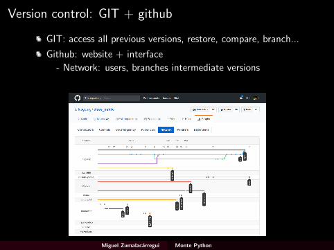
Version control: GIT + github
GIT: access all previous versions, restore, compare, branch...
Github: website + interface
- Network: users, branches intermediate versions
- Issues: troubleshooting, forum/improvements
Miguel Zumalacarregui Monte Python

Version control: GIT + github
GIT: access all previous versions, restore, compare, branch...
Github: website + interface
- Network: users, branches intermediate versions
- Issues: troubleshooting, forum/improvements
Miguel Zumalacarregui Monte Python
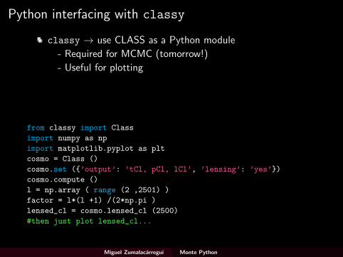
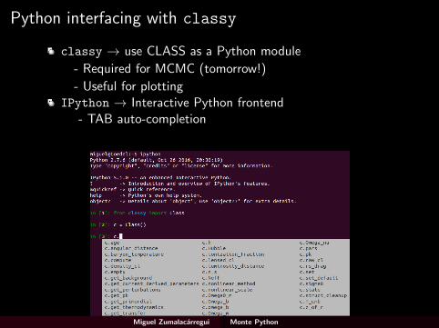
Python interfacing with classy
classy → use CLASS as a Python module
- Required for MCMC (tomorrow!)
- Useful for plotting
IPython → Interactive Python frontend- TAB auto-completion
Jupyter → Notebook interface (Julia+Pyton+R)
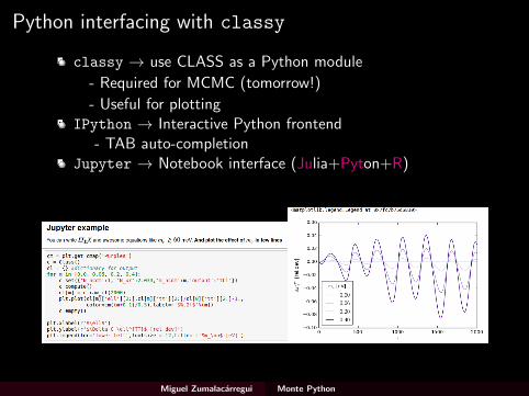
from classy import Class
import numpy as np
import matplotlib.pyplot as plt
cosmo = Class ()
cosmo.set (’output’: ’tCl, pCl, lCl’, ’lensing’: ’yes’)
cosmo.compute ()
l = np.array ( range (2 ,2501) )
factor = l*(l +1) /(2*np.pi )
lensed_cl = cosmo.lensed_cl (2500)
#then just plot lensed_cl...
Miguel Zumalacarregui Monte Python
Python interfacing with classy
classy → use CLASS as a Python module
- Required for MCMC (tomorrow!)
- Useful for plottingIPython → Interactive Python frontend
- TAB auto-completion
Jupyter → Notebook interface (Julia+Pyton+R)
Miguel Zumalacarregui Monte Python
Python interfacing with classy
classy → use CLASS as a Python module
- Required for MCMC (tomorrow!)
- Useful for plottingIPython → Interactive Python frontend
- TAB auto-completionJupyter → Notebook interface (Julia+Pyton+R)
Miguel Zumalacarregui Monte Python

Monte Python
from cosmology back to fundamental physicsPLANCK
Miguel Zumalacarregui Monte Python
DISCLAIMER: Short time!
. 3h course ⇒ overview and basic usage
Learn further:
MontePython slides by Sebastien Clesse ( 1h?)https://lesgourg.github.io/class-tour/16.06.02_Lisbon_intro.pdf
MontePython course (∼ 5h)https://lesgourg.github.io/class-tour-Tokyo.html
Links to extra resources in exercise sheet
IMPORTANT DISCLAIMER:
↓ I’m mainly a user with little experience developing!
↑ Help from experts:
Thejs Brinckmann, Carlos Garcia, Deanna Hooper & Vivian Poulin
Miguel Zumalacarregui Monte Python

Fundamental physics and cosmology
10-4 10-3 10-2 10-1 100101
102
103
104
105
P(k
) [1/
Mpc
3]
mν =(mi ,0,0)
10-4 10-3 10-2 10-1 100
k [1/Mpc]
50
40
30
20
10
0
rel.
dev.
[%]
mi [eV]0.00
0.25
0.50
0.75
1.00
Initial conditions, Dark Matter, Neutrinos, Dark Energy, Gravity...
Miguel Zumalacarregui Monte Python
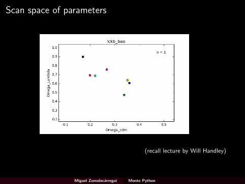
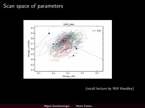
Scan space of parameters
(recall lecture by Will Handley)
Miguel Zumalacarregui Monte Python

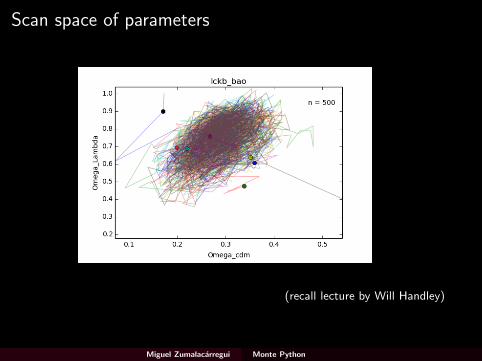
Scan space of parameters
(recall lecture by Will Handley)
Miguel Zumalacarregui Monte Python

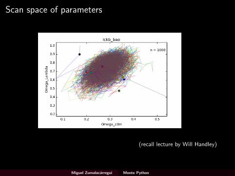
Scan space of parameters
(recall lecture by Will Handley)
Miguel Zumalacarregui Monte Python

Scan space of parameters
(recall lecture by Will Handley)
Miguel Zumalacarregui Monte Python

Scan space of parameters
(recall lecture by Will Handley)
Miguel Zumalacarregui Monte Python
Scan space of parameters
(recall lecture by Will Handley)
Miguel Zumalacarregui Monte Python
Scan space of parameters
(recall lecture by Will Handley)
Miguel Zumalacarregui Monte Python
Scan space of parameters
(recall lecture by Will Handley)
Miguel Zumalacarregui Monte Python
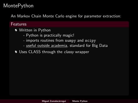
MontePython
An Markov Chain Monte Carlo engine for parameter extraction:
Features
Written in Python- Python is practically magic!- imports routines from numpy and scipy
- useful outside academia, standard for Big Data
Uses CLASS through the classy wrapper
Modular, easy to add- likelihoods for new experiments- features for sampling, plotting...
Easy to use, intensively documented
Parallelization is optional- simpler to install- runs in old/separate computers, short queue
Miguel Zumalacarregui Monte Python
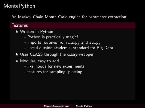
MontePython
An Markov Chain Monte Carlo engine for parameter extraction:
Features
Written in Python- Python is practically magic!- imports routines from numpy and scipy
- useful outside academia, standard for Big Data
Uses CLASS through the classy wrapper
Modular, easy to add- likelihoods for new experiments- features for sampling, plotting...
Easy to use, intensively documented
Parallelization is optional- simpler to install- runs in old/separate computers, short queue
Miguel Zumalacarregui Monte Python
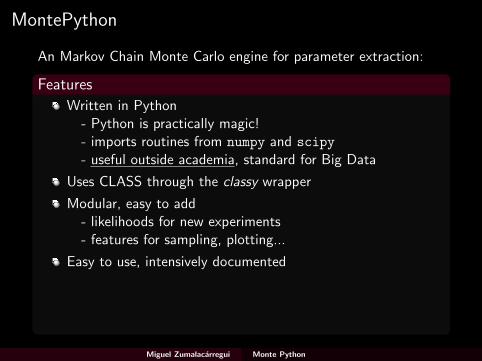
MontePython
An Markov Chain Monte Carlo engine for parameter extraction:
Features
Written in Python- Python is practically magic!- imports routines from numpy and scipy
- useful outside academia, standard for Big Data
Uses CLASS through the classy wrapper
Modular, easy to add- likelihoods for new experiments- features for sampling, plotting...
Easy to use, intensively documented
Parallelization is optional- simpler to install- runs in old/separate computers, short queue
Miguel Zumalacarregui Monte Python
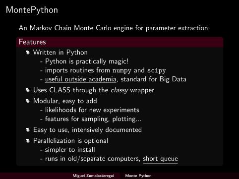

Modular Structure
(from B. Audren’s Monte Python slides)
Miguel Zumalacarregui Monte Python
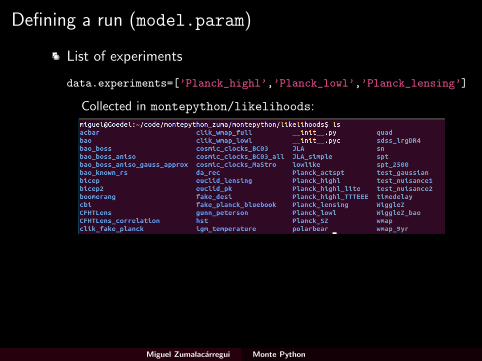
Defining a run (model.param)
List of experiments
data.experiments=[’Planck_highl’,’Planck_lowl’,’Planck_lensing’]
Collected in montepython/likelihoods:
Miguel Zumalacarregui Monte Python

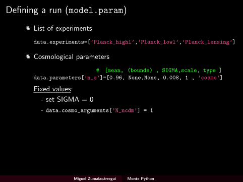
Defining a run (model.param)
List of experiments
data.experiments=[’Planck_highl’,’Planck_lowl’,’Planck_lensing’]
Cosmological parameters
# [mean, (bounds) , SIGMA,scale, type ]
data.parameters[’n_s’]=[0.96, None,None, 0.008, 1 , ’cosmo’]
Fixed values:
- set SIGMA = 0
- data.cosmo_arguments[’N_ncdm’] = 1
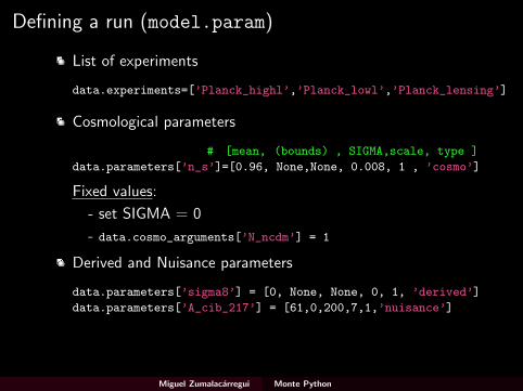
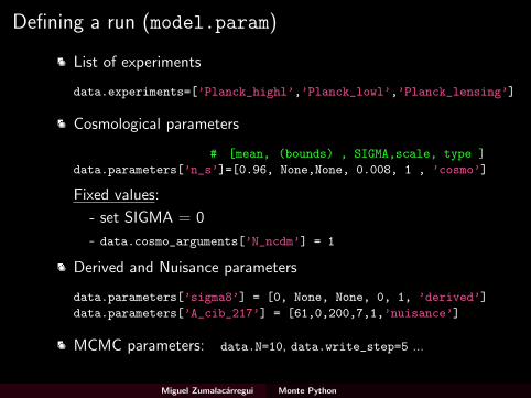
Derived and Nuisance parameters
data.parameters[’sigma8’] = [0, None, None, 0, 1, ’derived’]
data.parameters[’A_cib_217’] = [61,0,200,7,1,’nuisance’]
MCMC parameters: data.N=10, data.write_step=5 ...
Miguel Zumalacarregui Monte Python
Defining a run (model.param)
List of experiments
data.experiments=[’Planck_highl’,’Planck_lowl’,’Planck_lensing’]
Cosmological parameters
# [mean, (bounds) , SIGMA,scale, type ]
data.parameters[’n_s’]=[0.96, None,None, 0.008, 1 , ’cosmo’]
Fixed values:
- set SIGMA = 0
- data.cosmo_arguments[’N_ncdm’] = 1
Derived and Nuisance parameters
data.parameters[’sigma8’] = [0, None, None, 0, 1, ’derived’]
data.parameters[’A_cib_217’] = [61,0,200,7,1,’nuisance’]
MCMC parameters: data.N=10, data.write_step=5 ...
Miguel Zumalacarregui Monte Python
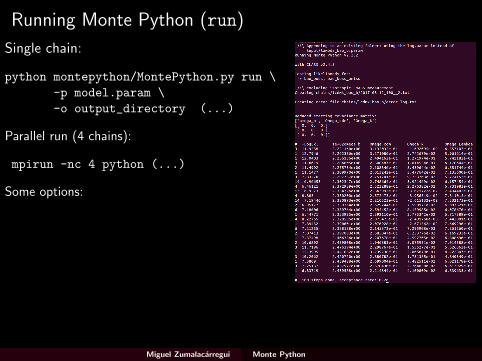
Running Monte Python (run)
Single chain:
python montepython/MontePython.py run \
-p model.param \
-o output_directory (...)
Parallel run (4 chains):
mpirun -nc 4 python (...)
Some options:
-N → # points
-C → covariance matrix
-r → restart from last point of chain
--update → update sampling + covariance
All options explained
python montepython/MontePython.py info --help
Miguel Zumalacarregui Monte Python
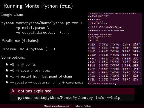
Running Monte Python (run)
Single chain:
python montepython/MontePython.py run \
-p model.param \
-o output_directory (...)
Parallel run (4 chains):
mpirun -nc 4 python (...)
Some options:
-N → # points
-C → covariance matrix
-r → restart from last point of chain
--update → update sampling + covariance
All options explained
python montepython/MontePython.py info --help
Miguel Zumalacarregui Monte Python
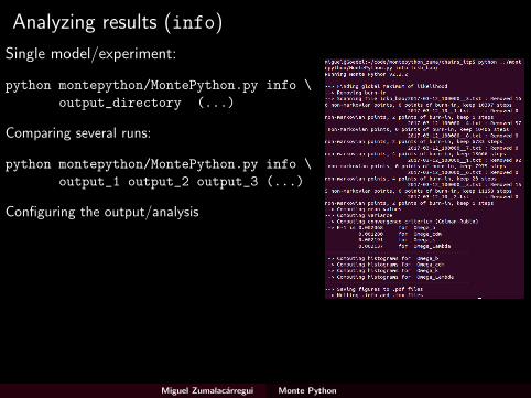
Analyzing results (info)
Single model/experiment:
python montepython/MontePython.py info \
output_directory (...)
Comparing several runs:
python montepython/MontePython.py info \
output_1 output_2 output_3 (...)
Configuring the output/analysis
--extra → file with plot options
--bins → # bins for posterior
--all → plot every subplot separately
--no-mean → only marginalized in 1D
All options explained
python montepython/MontePython.py info --help
Miguel Zumalacarregui Monte Python

A very minimal run
Write lckb.param:
data.experiments=[’bao_boss’,’bao_boss_aniso’]
#Cosmo parameteress [mean, min, max, sigma, scale, type]
data.parameters[’Omega_b’] = [0.045,0.01, None,0.01,1,’cosmo’]
data.parameters[’Omega_cdm’] = [0.3, 0, None, 0.1, 1, ’cosmo’]
data.parameters[’Omega_k’] = [0.0, -0.5, 0.5, 0.1, 1, ’cosmo’]
#Fixed parameters (sigma = 0)
data.parameters[’H0’] = [67.8, None, None, 0, 1, ’cosmo’]
data.cosmo_arguments[’YHe’] = 0.24
#derived parameters
data.parameters[’Omega_Lambda’] = [1,None,None,0,1,’derived’]
#mcmc parameters
data.N=10
data.write_step=5
Run ∼ 7 chains with
python montepython/MontePython.py run -o chains/lckb_bao \
-p lckb_param --update 300 -N 100000
Miguel Zumalacarregui Monte Python
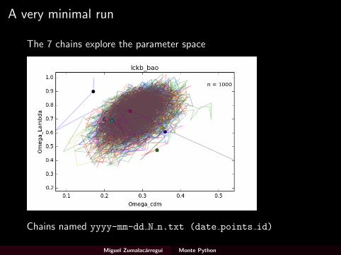
A very minimal run
The 7 chains explore the parameter space
Chains named yyyy-mm-dd N n.txt (date points id)
Miguel Zumalacarregui Monte Python
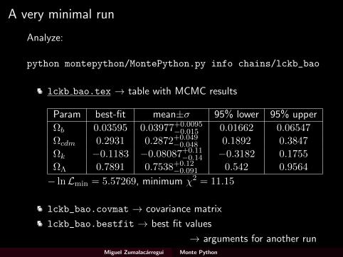
A very minimal run
Analyze:
python montepython/MontePython.py info chains/lckb_bao
lckb bao.tex → table with MCMC results
Param best-fit mean±σ 95% lower 95% upper
Ωb 0.03595 0.03977+0.0095−0.015 0.01662 0.06547
Ωcdm 0.2931 0.2872+0.049−0.048 0.1892 0.3847
Ωk −0.1183 −0.08087+0.11−0.14 −0.3182 0.1755
ΩΛ 0.7891 0.7538+0.12−0.091 0.542 0.9564
− lnLmin = 5.57269, minimum χ2 = 11.15
lckb_bao.covmat → covariance matrix
lckb_bao.bestfit → best fit values
→ arguments for another runMiguel Zumalacarregui Monte Python

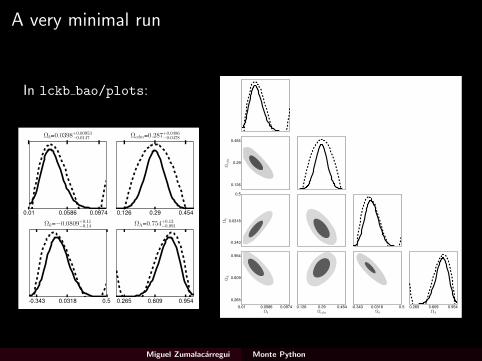
A very minimal run
In lckb bao/plots:
0.01 0.0586 0.0974
Ωb=0.0398+0.00953−0.0147
0.126 0.29 0.454
Ωcdm=0.287+0.0486−0.0478
-0.343 0.0318 0.5
Ωk=−0.0809+0.11−0.14
0.265 0.609 0.954
ΩΛ=0.754+0.12−0.091
Miguel Zumalacarregui Monte Python
A very minimal run
In lckb bao/plots:
0.01 0.0586 0.0974
Ωb=0.0398+0.00953−0.0147
0.126 0.29 0.454
Ωcdm=0.287+0.0486−0.0478
-0.343 0.0318 0.5
Ωk=−0.0809+0.11−0.14
0.265 0.609 0.954
ΩΛ=0.754+0.12−0.091
0.126
0.29
0.454
Ωcdm
-0.343
0.0318
0.5
Ωk
0.265 0.609 0.954ΩΛ
0.01 0.0586 0.0974Ωb
0.265
0.609
0.954
ΩΛ
0.126 0.29 0.454Ωcdm
-0.343 0.0318 0.5Ωk
Miguel Zumalacarregui Monte Python
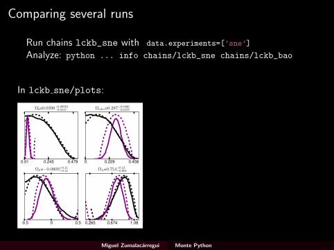
Comparing several runs
Run chains lckb_sne with data.experiments=[’sne’]
Analyze: python ... info chains/lckb_sne chains/lckb_bao
In lckb sne/plots:
0.01 0.245 0.479
Ωb=0.0398+0.00953−0.0147
0 0.229 0.458
Ωcdm=0.287+0.0486−0.0478
-0.5 0 0.5
Ωk=−0.0809+0.11−0.14
0.265 0.674 1.08
ΩΛ=0.754+0.12−0.091
Miguel Zumalacarregui Monte Python
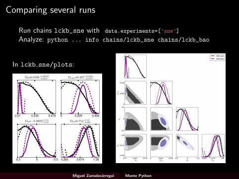
Comparing several runs
Run chains lckb_sne with data.experiments=[’sne’]
Analyze: python ... info chains/lckb_sne chains/lckb_bao
In lckb sne/plots:
0.01 0.245 0.479
Ωb=0.0398+0.00953−0.0147
0 0.229 0.458
Ωcdm=0.287+0.0486−0.0478
-0.5 0 0.5
Ωk=−0.0809+0.11−0.14
0.265 0.674 1.08
ΩΛ=0.754+0.12−0.091
0
0.229
0.458
Ωcdm
-0.5
0
0.5
Ωk
0.265 0.674 1.08ΩΛ
0.01 0.245 0.479Ωb
0.265
0.674
1.08
ΩΛ
0 0.229 0.458Ωcdm
-0.5 0 0.5Ωk
lckb snelckb bao
Miguel Zumalacarregui Monte Python
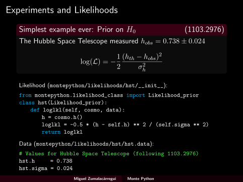
Experiments and Likelihoods
Simplest example ever: Prior on H0 (1103.2976)
The Hubble Space Telescope measured hobs = 0.738± 0.024
log(L) = −1
2
(hth − hobs)2
σ2h
Likelihood (montepython/likelihoods/hst/__init__):
from montepython.likelihood_class import Likelihood_prior
class hst(Likelihood_prior):
def loglkl(self, cosmo, data):
h = cosmo.h()
loglkl = -0.5 * (h - self.h) ** 2 / (self.sigma ** 2)
return loglkl
Data (montepython/likelihoods/hst/hst.data):
# Values for Hubble Space Telescope (following 1103.2976)
hst.h = 0.738
hst.sigma = 0.024
Miguel Zumalacarregui Monte Python

Likelihood rules
Likelihoods in directory montepython/likelihoods/l_name
Needed files: __init__.py and l_name.data
__init__.py defines a class, inheriting from Likelihood
Contains function loglkl → log(L)
Introducing your own Likelihoods
Follow the above rules
Inspire yourself with the examples
∃ similar likelihood? → you can inherit its methods!
You can use additional python packages
(See also B. Audren’s lecture on likelihoods)
Miguel Zumalacarregui Monte Python
Conclusions
Brings all the power of CLASS to Python
Easy to run chains and analyze likelihoods
Many available experiments
Advantages from object oriented features in python
- Add likelihoods
- Add samplers or other features
This just scratches the surface, many more options!
(See also B. Audren’s slides)
Miguel Zumalacarregui Monte Python
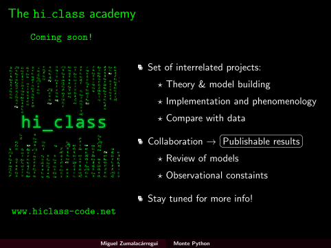
The hi class academy
Coming soon!
www.hiclass-code.net
Set of interrelated projects:
? Theory & model building
? Implementation and phenomenology
? Compare with data
Collaboration → Publishable results
? Review of models
? Observational constaints
Stay tuned for more info!
Miguel Zumalacarregui Monte Python


![DL MONTE: A multipurpose code for Monte Carlo simulation a ... · multi-histogram reweighting analysis method [37] as an extensible Python API class, as well as a self-contained weighted](https://static.fdocuments.us/doc/165x107/5e0be33195a4b31bf344deec/dl-monte-a-multipurpose-code-for-monte-carlo-simulation-a-multi-histogram-reweighting.jpg)