LECTURE NOTES

FYS 4550/FYS9550 - EXPERIMENTAL HIGH ENERGY PHYSICS

AUTUMN 2014

PART II MONTE CARLO TECHNIQUES

A. STRANDLIE

GJØVIK UNIVERSITY COLLEGE

AND UNIVERSITY OF OSLO

Monte Carlo • Monte Carlo techniques are very popular for several applications:

– Solving difficult integrals – Sampling from probability distributions

• Direct sampling from desired distributions • Markov chain Monte Carlo, sampling from equilibrium distributions defined

by transition probabilities between different states • Latter used for instance in statistical physics

• Will in this course focus on how to generate random numbers from a set of probability distributions – Monte Carlo generation of various processes in physics analyses – Simulation of tracks through detectors and the subsequent detector

response • Invaluable tool for designing detectors, understanding detector performance,

evaluating performance of track and vertex reconstruction algorithms etc.

Monte Carlo • Basic assumption: having a good and reliable generator of uniform

distribution between 0 and 1! – Generated distribution should really be flat – Generated numbers should be statistically independent

• No random number generator on a computer can fully satisfy these needs – After all some (deterministic) algorithm creates the ”random” numbers

• But there exist algorithms which for all practical purposes create numbers according to the desired properties – RANLUX – Lagged-Fibonacci – See references in Particle Data Book chap. 34

Monte Carlo • Inverse transform method • Given a probability density function (pdf) f(x) which we want to

generate random numbers from • The cumulative distribution function (cdf) is u=F(x)=P(X≤x) • The value u is itself a random variable following the uniform

distribution

Monte Carlo • Proof:

• The cdf, G(u), is linear, implying that the pdf (the derivative of the cdf), g(u), is flat

• So, assuming that the inverse cdf is available (either analytically or numerically), random numbers from f(x) can be generated by – Draw a number u from the uniform distribution – Calculate the corresponding value x from the inverse cdf – And that’s it

• Similar approach followed for a discrete distribution (see Particle Data Book and lowermost figure on previous slide)

uuFFxFxXPuUPuG ===≤=≤= − ))(()()()()( 1

Monte Carlo • Acceptance-rejection method (Von Neumann) • Illustration of approach:

Monte Carlo • Create ”envelope” Ch(x) (C>1) as illustrated in the figure, where h(x)

is a uniform distribution (a) or a normalized sum of uniform distributions (b)

• Assume that the desired f(x) can be calculated for all relevant values of x

• Sampling from f(x) is then achieved by – Draw x according to h(x) – Draw a number u from the standard, uniform distribution – If uCh(x)≤f(x), accept x, if not, reject x and try again

• Such a procedure repeated many times will populate the area below f(x) in a uniform way – Therefore x is indeed distributed according to f(x)

Monte Carlo • Efficiency (ratio of accepted trials to all trials) is equal to ratio of

areas – Must be 1/C

• High efficiency implies that envelope must follow f(x) as closely as possible

• Generating x according to the above-defined algorithm is an example of the concept of importance sampling – Region of largest importance of x (i.e. region with highest probability) is

sampled most often • Quiz: how does one sample from a normalized sum of uniform

distributions?

Monte Carlo • Will in the following look at a number of specific distributions and

how to generate samples from them • Very clear prescriptions are given in chap. 34.4 in the Particle Data

Book, will in general not repeat them here • Not considered essential to prove the prescriptions

– Except a few examples shown in these notes – The interested reader is referred to the cited literature in chap. 34.4 for

further details

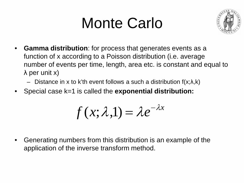
Monte Carlo • Gamma distribution: for process that generates events as a

function of x according to a Poisson distribution (i.e. average number of events per time, length, area etc. is constant and equal to λ per unit x) – Distance in x to k’th event follows a such a distribution f(x;λ,k)

• Special case k=1 is called the exponential distribution:

• Generating numbers from this distribution is an example of the application of the inverse transform method.

xexf λλλ −=)1,;(

Monte Carlo • Find F(x) by integrating f(x) (and using the fact that also 1-u is

uniformly distributed):

• Draw u from a uniform distribution • Calculate x from the above formula • This x should follow the exponential distribution • Example: λ=1. Generate various numbers from the distribution, plot

in histogram and compare with true pdf

uxeu

uedxxfxF

x

xx

ln1

11')'()(0

λλ

λ

−=⇒=⇒

−=−==

−

−∫

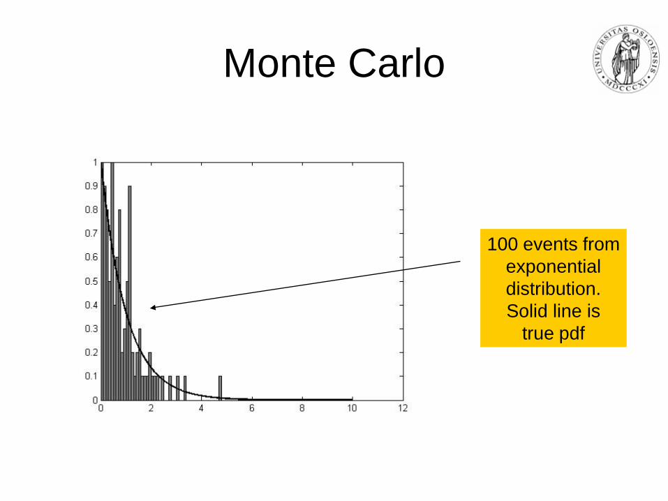
Monte Carlo

100 events from exponential distribution. Solid line is

true pdf

Monte Carlo

500 events 1000 events

5000 events 10000 events

Monte Carlo

100000 events 1000000 events

Monte Carlo • Gaussian distribution • Not easy to use inverse transform method for one-dimensional

distribution, because there is no closed expression for the cdf • Trick: use two-dimensional Gaussian f(x,y) and express in azimuthal

coordinates (r,φ) – Transform to these variables in the standard way – Integrate to obtain the cdf F(r) – Invert such that r is expressed as a function of a uniform u – Draw u from flat distribution and calculate r(u) – Draw another u from a flat distribution and multiply by 2π to obtain φ

from a flat distribution between 0 and 2π – Calculate x=r cos φ and y=r sin φ – These are now uncorrelated and independent variables, following a

standard Gaussian distribution – Generating histograms as in the previous example

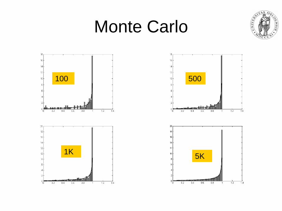
Monte Carlo

100 500

1K 5K

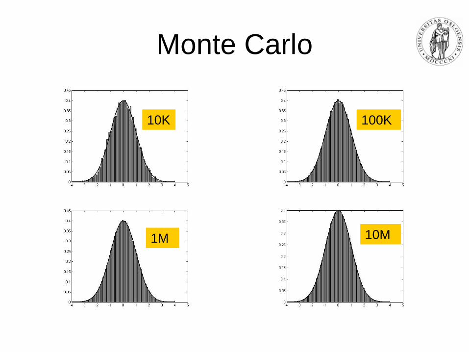
Monte Carlo

10K 100K

1M 10M

Monte Carlo • Faster algorithm based on acceptance-rejection principle is also

available • Multivariate Gaussian with covariance matrix V can also be

simulated – Using Cholesky decomposition of V into product of unique lower

triangular matrix L with its own transpose – See 34.4.4 in Particle Data Book for details

• Chisquare, binomial, Poisson and Student’s t and distributions – 34.4.5, 34.4.7, 34.4.8 and 34.4.9 in Particle Data Book

Monte Carlo • Example: simulation of bremsstrahlung energy loss for electrons • Useful when making fast simulation of electron tracks through tracking

detector setup • Model of pdf (due to Bethe and Heitler) of fractional energy loss z after

having penetrated layer of material with radiation thickness t

[ ]( )

)2ln/(ln)(

12ln/

tzzf

t

Γ−

=−

Monte Carlo • Transformation to x=-ln(z) gives the pdf

which is a special case of the gamma distribution with λ=1 and k=t/ln2 • Sampling from f(z) can therefore be done by sampling x from

gamma distribution (34.4.6) and transforming to z by direct calculation of z(x)

( )

)2ln/()(

12ln/

texxg

xt

Γ=

−−

)(),;(

1

kexkxg

xkk

Γ=

−− λλλ

Monte Carlo

100 500

1K 5K

Monte Carlo

100K 10K