Monte Carlo Simulation of Learning in the Hawk-Dove … Carlo Simulation of Learning in the Hawk ......

Bernstein 1

Monte Carlo Simulation of Learning in

the Hawk-Dove Game

Alex Bernstein

Washington University in St. Louis

March 18, 2014

Abstract

The goal of this paper is to construct a Monte Carlo simulation in order to systematically

analyze how equilibria arise in evolutionary games. I examine the “Hawk-Dove” game, where

the equilibria are already understood, in order to judge whether the model matches the analytic

expectations. In all situations, the model approaches the expected results.

Bernstein 2

1. Introduction

Game-theoretic models of learning and evolution are a relatively recent development that

alter some of the foundational assumptions of Game Theory. Rather than considering supremely

rational actors whose rationality is well known, Evolutionary Game Theory examines “less than

fully rational players [who] grope for optimality over time.” (Fudenberg and Levine, 1998).

One of the most common games in Evolutionary Game Theory is the Hawk-Dove game.

First introduced in 1973 by Maynard Smith, the Hawk-Dove game is a zero sum, symmetric

game in which two players contest a single resource valued at V. Players can either play the

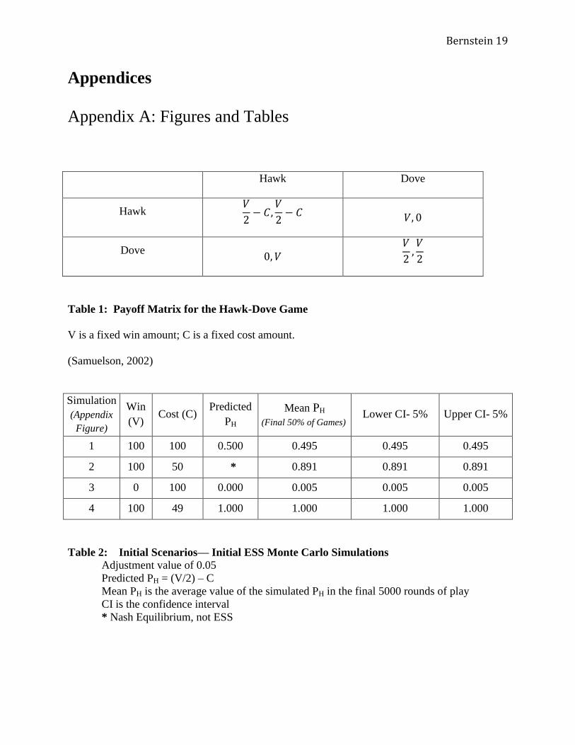
aggressive “Hawk” strategy, or the pacifist “Dove” strategy. (c.f. Table 1 for the payoff matrix)

If one player plays “Hawk” and the other “Dove,” the former earns the entire payoff, V, while the

latter earns 0. If both players play “Dove,” they split the resource, and earn

. If both players

play “Hawk,” they also split the resource, but each incurs the cost, C, earning

.

Evolutionary Game Theory itself has many useful applications in modern economic

analysis. Although originally developed to help understand evolutionary biology, these same

concepts have been adapted to understand selection among multiple equilibria and adaptation,

given random matching and myopic memory among the player population. (Friedman, 1998)

The Hawk-Dove game, while relatively uncommon in terms of economic applications, has been

applied to understand legal compliance. Behavioral experiments using the Hawk-Dove game

have demonstrated that it is an effective way to model individual decision-making in the face of

precedents. (McAdams and Nadler, 2005) Another potential use for Hawk-Dove game that has

not been heavily investigated is patent litigation, which is closely related to legal compliance. If

one assumes a perfectly competitive patent market, in which players must “use” the intellectual

Bernstein 3

property of another firm, there are clear similarities to the Hawk-Dove game. The Hawk/Dove

situation can clearly represent a firm threating legal activity and its opponent settling, whereas

the Dove/Dove situation is a mutual, non-aggression pact of sorts. The Hawk/Hawk situation is

a bit more troublesome, because of the zero-sum nature of the Hawk-Dove game. It could

represent a retaliatory strategy, assuming each agent has potential intellectual property

advantages over its opponent. The Hawk/Hawk situation then could represent both an initial

lawsuit and a countersuit, in which each firm’s overall situation relative to one another doesn’t

really change, but in which they both incur legal costs.

The purpose of this paper is to conduct a Monte Carlo simulation in order to mimic these

natural processes and check the convergence against the predicted theoretical results. As

described in the next section, the equilibria of the Hawk-Dove game are well understood. In

order to construct this model, a simulation was written in Java and run for different values of V

and C. The simulation allowed a player to learn from its results over a fixed set of games. For

consistency, I chose to set this number at 10, although I did investigate longer sets in order to

understand the robustness of my model. This allowed for a “fictitious play” type situation to

develop, which will be discussed further in Section 2. This Monte Carlo simulation approaches

expected values in all situations, and the convergence is closer to expected values if the number

of games over which learning occurs is extended.

2. Literature Review

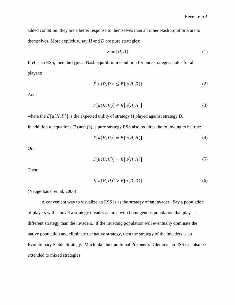
It is important to understand the criteria for equilibria in Evolutionary Game Theory,

which are stricter than for more traditional games. These equilibrium strategies, known as

Evolutionary Stable Strategies, or ESS, are similar to Nash Equilibrium strategies but with an

Bernstein 4

added condition; they are a better response to themselves than all other Nash Equilibria are to

themselves. More explicitly, say H and D are pure strategies:

(1)

If H is an ESS, then the typical Nash equilibrium condition for pure strategies holds for all

players:

(2)

And:

(3)

where the is the expected utility of strategy H played against strategy D.

In addition to equations (2) and (3), a pure strategy ESS also requires the following to be true:

(4)

Or:

(5)

Then:

(6)

(Neugerbauer et. al, 2006)

A convenient way to visualize an ESS is as the strategy of an invader. Say a population

of players with a novel a strategy invades an area with homogenous population that plays a

different strategy than the invaders. If the invading population will eventually dominate the

native population and eliminate the native strategy, then the strategy of the invaders is an

Evolutionary Stable Strategy. Much like the traditional Prisoner’s Dilemma, an ESS can also be

extended to mixed strategies.

Bernstein 5

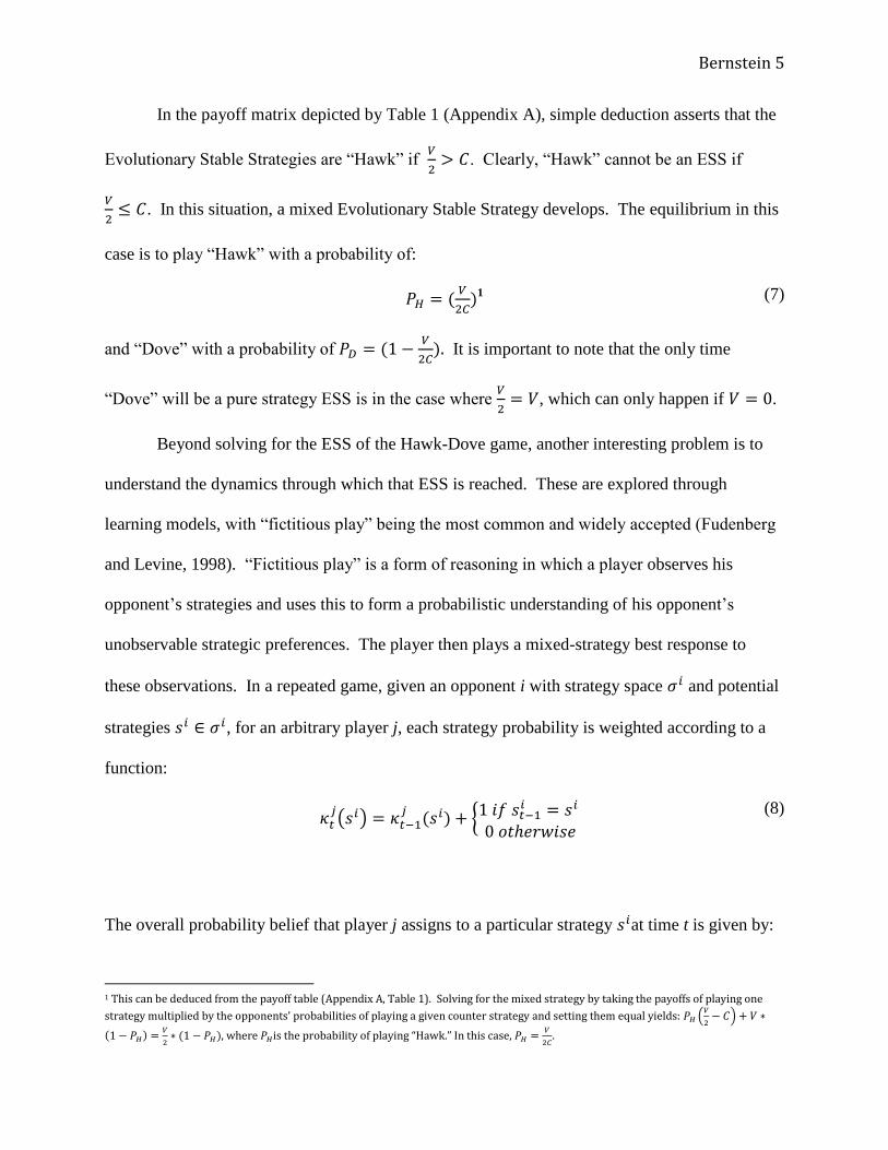
In the payoff matrix depicted by Table 1 (Appendix A), simple deduction asserts that the

Evolutionary Stable Strategies are “Hawk” if

. Clearly, “Hawk” cannot be an ESS if

. In this situation, a mixed Evolutionary Stable Strategy develops. The equilibrium in this

case is to play “Hawk” with a probability of:

1

(7)

and “Dove” with a probability of

It is important to note that the only time

“Dove” will be a pure strategy ESS is in the case where

, which can only happen if .

Beyond solving for the ESS of the Hawk-Dove game, another interesting problem is to

understand the dynamics through which that ESS is reached. These are explored through

learning models, with “fictitious play” being the most common and widely accepted (Fudenberg

and Levine, 1998). “Fictitious play” is a form of reasoning in which a player observes his

opponent’s strategies and uses this to form a probabilistic understanding of his opponent’s

unobservable strategic preferences. The player then plays a mixed-strategy best response to

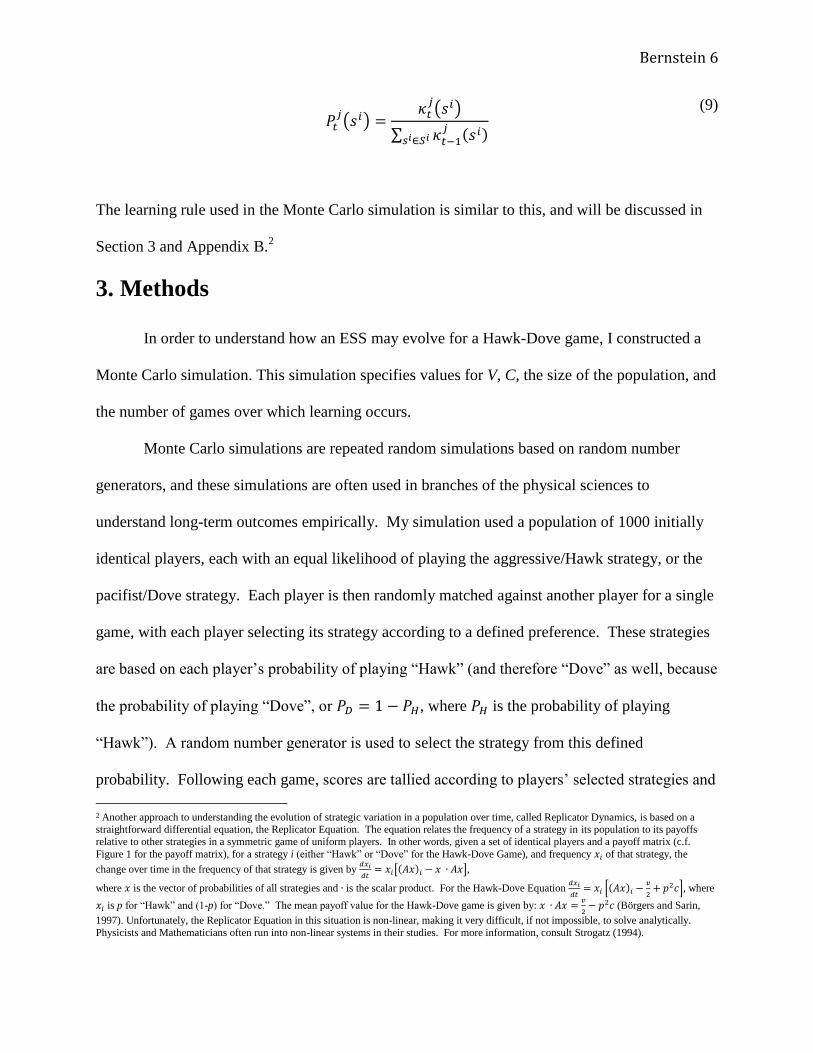
these observations. In a repeated game, given an opponent i with strategy space and potential

strategies , for an arbitrary player j, each strategy probability is weighted according to a

function:

(8)

The overall probability belief that player j assigns to a particular strategy at time t is given by:

1 This can be deduced from the payoff table (Appendix A, Table 1). Solving for the mixed strategy by taking the payoffs of playing one

strategy multiplied by the opponents’ probabilities of playing a given counter strategy and setting them equal yields:

, where is the probability of playing “Hawk.” In this case,

.

Bernstein 6

(9)

The learning rule used in the Monte Carlo simulation is similar to this, and will be discussed in

Section 3 and Appendix B.2

3. Methods

In order to understand how an ESS may evolve for a Hawk-Dove game, I constructed a

Monte Carlo simulation. This simulation specifies values for V, C, the size of the population, and

the number of games over which learning occurs.

Monte Carlo simulations are repeated random simulations based on random number

generators, and these simulations are often used in branches of the physical sciences to

understand long-term outcomes empirically. My simulation used a population of 1000 initially

identical players, each with an equal likelihood of playing the aggressive/Hawk strategy, or the

pacifist/Dove strategy. Each player is then randomly matched against another player for a single

game, with each player selecting its strategy according to a defined preference. These strategies

are based on each player’s probability of playing “Hawk” (and therefore “Dove” as well, because

the probability of playing “Dove”, or , where is the probability of playing

“Hawk”). A random number generator is used to select the strategy from this defined

probability. Following each game, scores are tallied according to players’ selected strategies and

2 Another approach to understanding the evolution of strategic variation in a population over time, called Replicator Dynamics, is based on a

straightforward differential equation, the Replicator Equation. The equation relates the frequency of a strategy in its population to its payoffs

relative to other strategies in a symmetric game of uniform players. In other words, given a set of identical players and a payoff matrix (c.f.

Figure 1 for the payoff matrix), for a strategy i (either “Hawk” or “Dove” for the Hawk-Dove Game), and frequency of that strategy, the

change over time in the frequency of that strategy is given by

,

where is the vector of probabilities of all strategies and is the scalar product. For the Hawk-Dove Equation

, where

is p for “Hawk” and (1-p) for “Dove.” The mean payoff value for the Hawk-Dove game is given by:

(Börgers and Sarin,

1997). Unfortunately, the Replicator Equation in this situation is non-linear, making it very difficult, if not impossible, to solve analytically.

Physicists and Mathematicians often run into non-linear systems in their studies. For more information, consult Strogatz (1994).

Bernstein 7

the payoff matrix for the Hawk-Dove game. Games are conducted so that each player plays a

game before any player plays again. Players remember both their strategy and their successes

over a fixed number of games. After the pre-determined number of games has elapsed, each

player adjusts its strategy according to how well the player did in the previous rounds over which

it is learning, given the strategies played in the prior set of games. This learning dynamic is

similar to the fictitious play dynamic described in the previous section, albeit with some

modifications. Rather than adjusting strategies immediately to the best response, each player

adjusts his strategy incrementally, by a small, pre-determined amount3. This differs from the

above description of fictitious play in that a player cannot immediately construct a best response.

This methodology simplifies the programming, but it also engenders a bias based on the player’s

experiences that may differ slightly in weight than if a true best response had been played.

Finally, it is important to note that each player does not keep a record of his entire history, but of

only a relatively small number of recent games. This, again, is to simplify the learning

algorithm, but it may also better reflect an agent’s tendency to favor more recent memories over

older ones. Because of these modifications to the principles of fictitious play, I expect to see the

simulated dominant strategies diverge slightly from expected values, matching the predicted

values the longer the learning period is extended.

The learning dynamic for adjusting strategies gauges how successful playing a

“collapsed” strategy of “Hawk” or “Dove” has been. In order to do this, the score earned when

playing a specific strategy is tallied and divided by the number of times that strategy has been

played. Whichever strategy was more successful, that is, scoring higher relative to its potential

score, (i.e. V each time for “Hawk” and

for each time “Dove” is played) increases in

3 I initially set to a change in probability of 0.05, but later varied it.

Bernstein 8

probability for the next round. Special cases are added to handle edge cases in the situations in

which all players converge to a pure strategy. A more detailed explanation of the learning

algorithm is available in Appendix B, and a numerical example, worked out for a single set of

games, is available in Appendix C. Similar simulations have been attempted before (Orzack and

Hines, 2005), although the focus in my work is somewhat different. In the cited example, the

authors simulated reproduction within populations of different strategies, rather than allowing

strategic adjustment, and tested for the existence of single ESS versus a “polymorphism,” or ESS

aggregate across the population. In general, I avoid such differences, and average players’

likelihood of playing “Hawk” and compare that average likelihood to the predicted ESS.

Therefore, an important distinction between this paper’s model and traditional models is

that, instead of examining a single agent playing against a single opponent in a repeated game,

this model evaluates the mean likelihood of the probability of playing “Hawk” by a population of

players. In this situation, not all players may reach the predicted ESS, given that they may be

forming an incomplete or inaccurate belief of the population, based on who they faced.

Nonetheless, the mean strategy should still converge to that ESS. Thus, while each individual

player may not reach the ESS, a stable state may still arise, with the average of all players’

converging to the predicted ESS. In order to examine the differences in strategies amongst the

players, I also recorded the standard deviation of the mean for each scenario.

The game is then repeated over 10,000 times, so each agent plays 10,000 games and

adjusts its strategy 1,000 times. Because the players are paired, this results in a total of 500,000

games played. The simulation is repeated varying the V and C values, starting with three

scenarios. In the first, V is worth 100 and the C is worth 100. Traditionally, this should mean

that a player is indifferent between “Hawk” and “Dove.” In the second, a V is worth 100 and the

Bernstein 9

C is zero. In this situation, according to traditional evolutionary Game Theory, the ESS is to

play “Hawk” with certainty. In the third scenario, I chose a V of 0 and a C of 100. The ESS in

this situation would be to play “Dove” with certainty. I then chose to run a simulation with a V

valued at 100 and a C valued at 49, in an attempt to verify the ESS when

.

Following these initial scenarios, a few more situations were examined, with intermediate

values. These situations all had a constant V value of 100. The values of C used were 60 and

200. Neither of these situations should result in a pure strategy ESS (either entirely “Hawk” or

entirely “Dove”). In these cases, the theoretical ESS are probabilities of playing “Hawk,” or

of 0.83 and 0.25, respectively.

I also chose to examine a situation in which . This situation is interesting because

it does not have an ESS. Against an opponent playing “Hawk,” a player should be indifferent

between playing “Hawk” or “Dove,” as both would have the same payoff. Nevertheless,

“Hawk” still wins against an opponent who plays “Dove.” In this case, the problem reduced to a

Prisoner’s Dilemma, in which the Dove/Dove situation maybe Pareto Optimal, but is not a Nash

Equilibrium. Hawk/Hawk is a weakly dominant Nash Equilibrium, because given an opponent

that plays “Hawk,” an agent is indifferent between playing “Hawk” or “Dove.”

Following these analyses, I examined the rate at which a population adapts to the ESS or

stable state. In order to do this, I focused on a single situation, with and and

varied some of the parameters. I extended the simulation so that each player plays 50,000

games, and altered the adaptation amount from 0.05 to 0.01 and 0.1, respectively. I ran these

simulations twice, for learning periods of both 10 and 50 games. I also ran the original version,

with the adaptation amount of 0.05 over 50,000 games to get a more direct comparison. I chose

to extend the number of games played in order to have a better long-term understanding of how

Bernstein 10

the learning parameters affect not only the eventual outcome, but also the rate of strategic

adjustment of the population.

4. Results (The results for all standard length games are in Appendix A, Table 2 and 3)

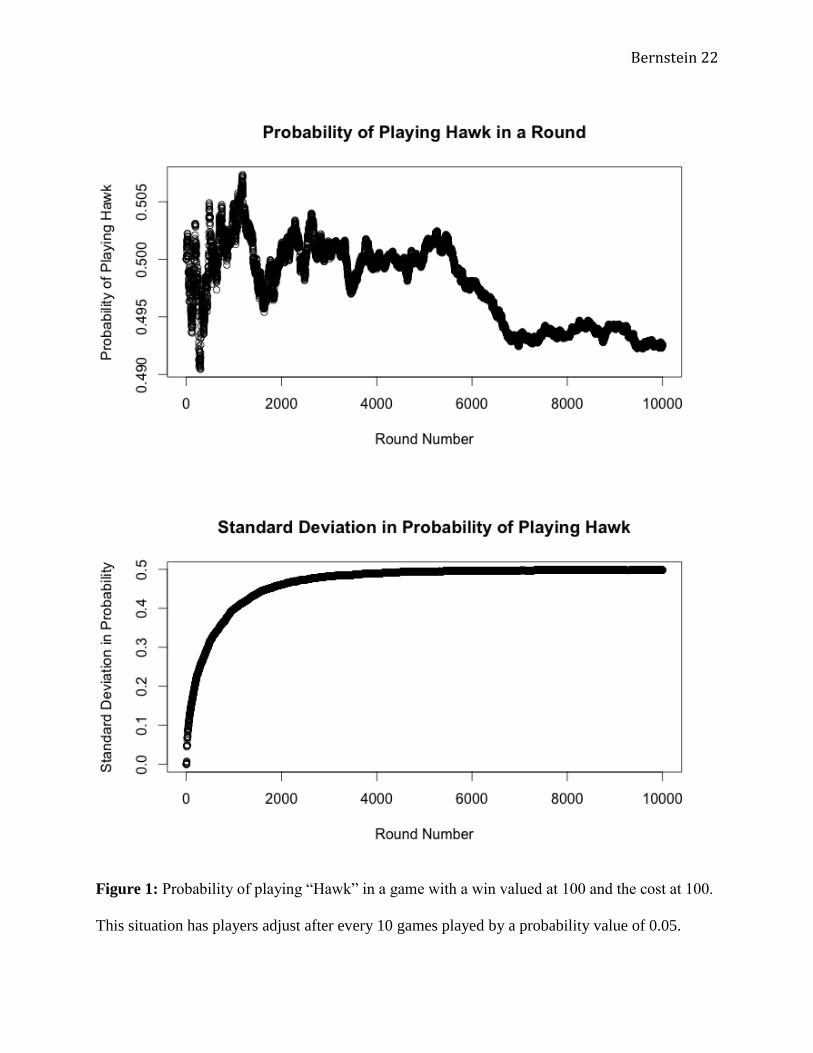
The first situation I analyzed had a V value of 100 and a C value of 100, so

, so

. In this situation, the expected ESS is to play “Hawk” with a probability of 0.5.

A graph of the mean likelihood of playing “Hawk” (Figure 1) shows that, after 10,000 rounds,

the probability of playing “Hawk” converges to about 49.5% over the latter half of the games.

The fact that the aggregate probability of playing “Hawk” decreased slightly over time suggests a

slight downward pressure away from the ESS, which may be an unforeseen consequence of the

random matching in the model. I also examined the graph of the standard deviation, which seem

to increase dramatically and then level off at about 0.5. This suggests that there is not one single

homogenous ESS developing, because the standard deviation grows with more games. Rather,

the agents in this game achieve an Evolutionarily Stable State that, in aggregate, resembles the

ideal Evolutionary Stable Strategy. As the standard deviation increases, it suggests a dichotomy

of sorts forming: certain agents heavily favor “Hawk” while others heavily favor “Dove.” This

is important, because it suggests that, although there are large variations within the population

itself, the average of all the participants’ likelihood of playing the “correct” strategy converges to

the predicted ESS.

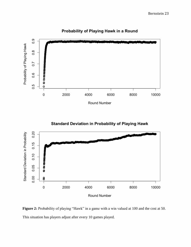
A similar situation occurred for the other initial cases. In the second trial (Figure 2), a V

of 100 and a C of 50 was used. In this case,

, implying that “Hawk” is a Nash Equilibrium

Bernstein 11

and not an ESS4. Nevertheless, the mean likelihood of playing “Hawk” did approach 0.9, with a

long term mean of 0.891 over the latter half of the games. The graph of the standard deviations

also showed a dramatic divergence in values as well. Because of the relatively high average

value of the mean, the large standard deviation suggests a few outlying values. This is especially

apparent in the later rounds of the simulation: a single standard deviation above the mean

probability is higher than the highest possible score within the simulation.5

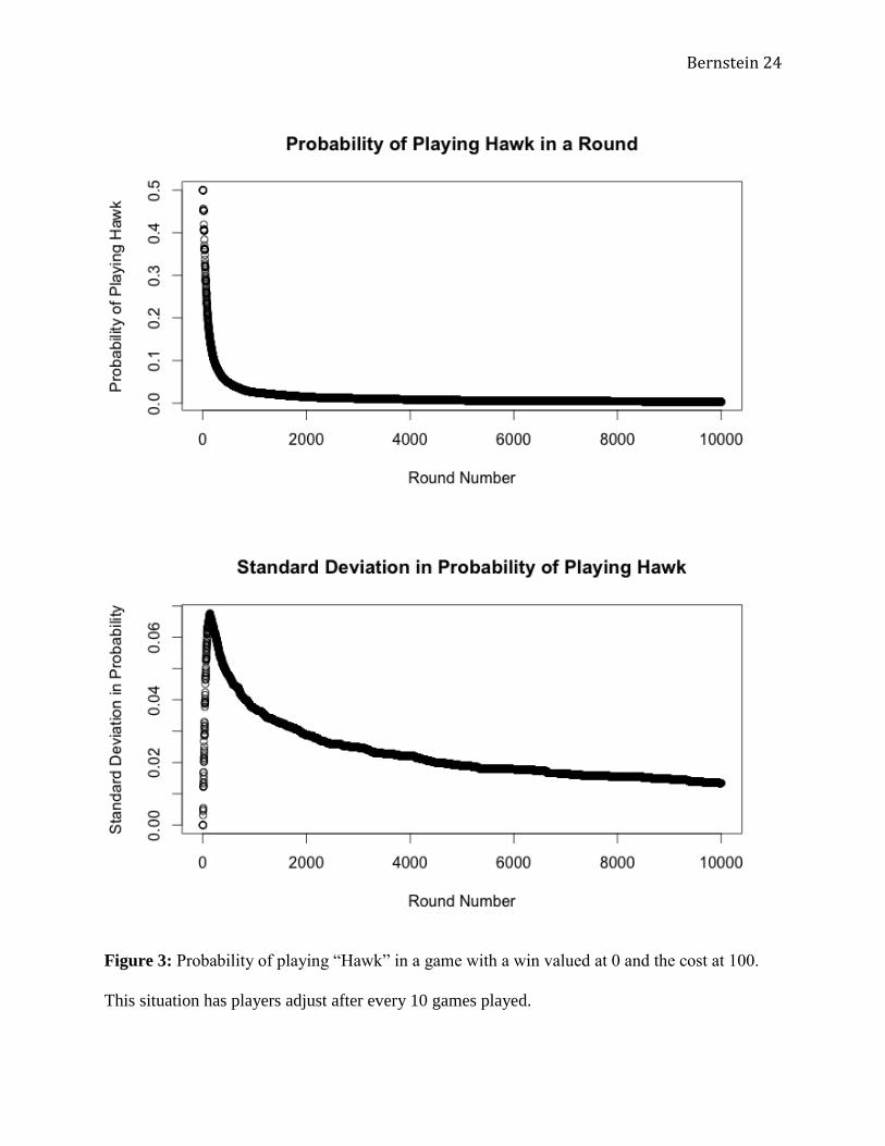
The third scenario (Figure 3) used a V valued at 0 and a C valued at 100. This was an

attempt to capture the dynamic that occurred when

. This is the only type of situation in

which playing “Dove” would be an ESS. As predicted, this is exactly what occurred: the mean

probability of playing “Hawk” rapidly approached 0, achieving a long-term mean of 0.005 over

the latter half of the games played. The standard deviations followed an expected pattern,

increasing dramatically then decreasing, as the probability of playing “Hawk” approaches 0 for

all agents. A similar but opposite situation occurred for the game with a V valued at 100 and a C

valued at 49 (Figure 4). This did reach the predicted ESS, with a certainty of playing “Hawk”

and with the standard deviation of the probability approaching 0, suggesting that all players

converged to these strategic probabilities.

The next two scenarios tested the intermediate probabilities, where

, resulting in a

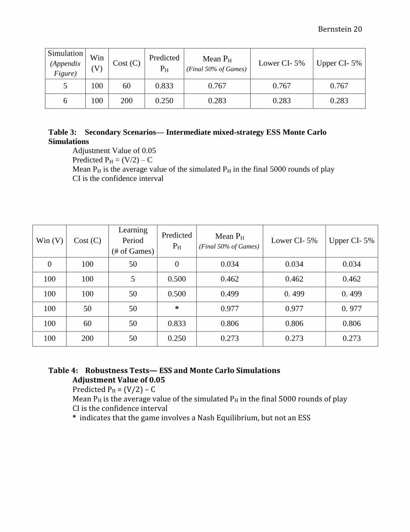
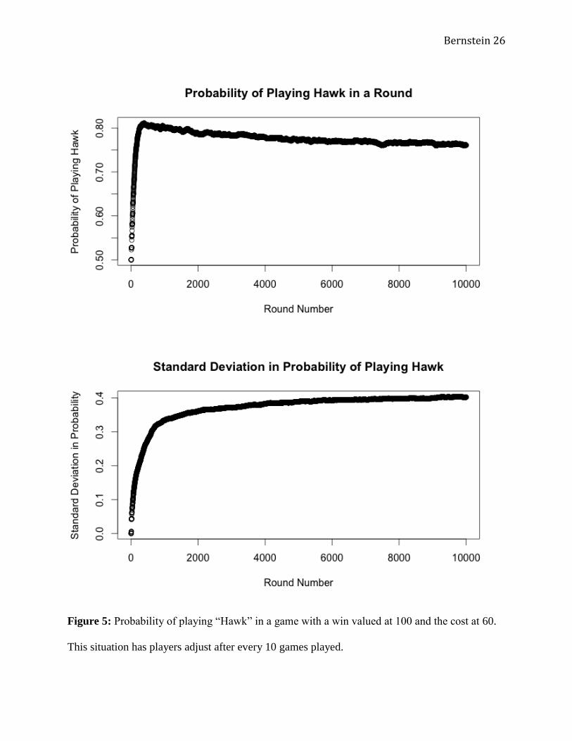
mixed strategy ESS. The first case (Figure 5) sets V equal to 100 and a C equal to 60. Solving

for the ESS with Equation (7) results in a probability of playing “Hawk” at about 0.833.6 While

this is not exactly what happened, the long-term mean was 0.767, which is reasonably close to

4 The game where and does not have an ESS because but . Nevertheless, playing “Hawk” still satisfies the conditions for a Nash Equilibrium. 5 For Example: the standard deviation for game 5000, was , whereas the mean for game 5000, or , was 0.893. Clearly, . Similar things happened in later games, with and 6 This value was found using Equation (8):

. This was reasonably close to the empirical result, with

.

Bernstein 12

the predicted outcome. The other simulation, with V valued at 100 and C at 200 (Figure 6) has a

theoretical ESS with a 0.25 probability of playing “Hawk”(Equation (8)). Again, the empirical

results were very close to these, with convergence to a long-term mean of a 0.283 probability of

playing “Hawk,” slightly above the predicted probability. The standard deviations in these

mixed strategy cases all followed a similar pattern as that observed in Figure 1. Again, this

suggests a large divergence in the strategies among players, with some diverging dramatically

from the predicted ESS. Nevertheless, the mean of all players’ probabilities to play “Hawk” or

“Dove” still approaches the predicted ESS.

5. Robustness and Further Discussion

In order to gauge the robustness of my simulation, I varied the number of games over

which learning occurs and the adjustment value following each learning cycle. I tested each

scenario by allowing a player to learn from every 50 games, or 200 times throughout the normal-

length simulation, and I also tested the scenario where each player learned after

every 5 games, or 2000 times throughout the simulation. The goal was to demonstrate that as

learning period increased, the empirical results more closely approach the predicted ESS. In

fact, by extending the learning period significantly, the results much more clearly approached the

predicted results. This supports the hypothesis that the average strategy approaches a best

response ESS the better the simulation’s approximation of a “fictitious play” scenario. The

results are in Table 4. These results were also supported when the adjustment value was altered,

as detailed next. Most situations reached a result much closer the predicted ESS when the

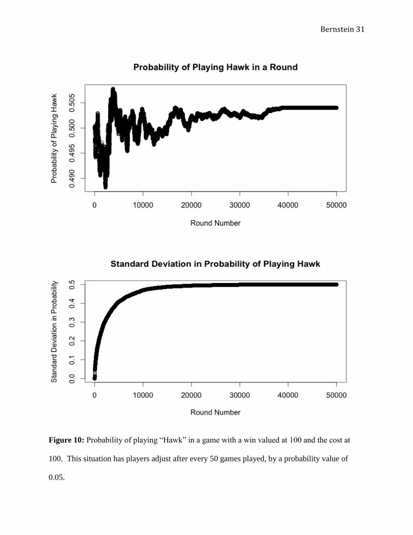
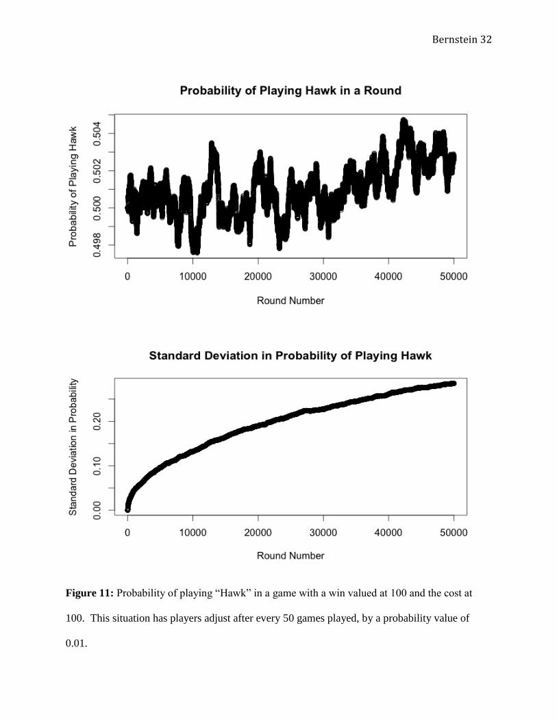
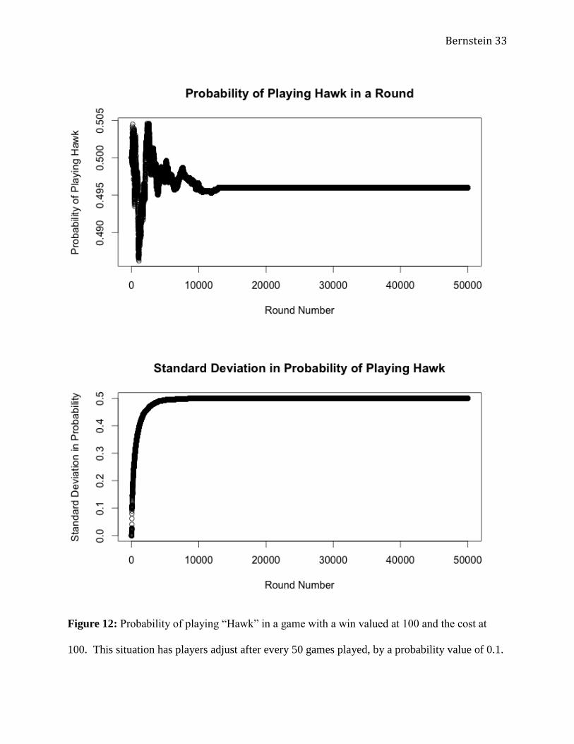
number of games over which learning occurred was extended (c.f. Figures 10,11,12 and Table

5).

Bernstein 13

The next scenario, along with all following scenarios, maintained the same values of

and for consistency, only adjusting the parameters for strategic adjustment

and number of games learned from. I altered these parameters in order to understand how

adjusting them affects both the result of the learning process and the rate at which the adjustment

happens. The results for all following trials are in Table 5. The first situation I examined

(Figure 7) simply extended the simulation modeled in Figure 1 by a factor of five. That is, it

involved 50,000 rather than 10,000 games, but learning still only took place over 10 games.

Interestingly, in this situation, the long-term steady state diverged somewhat more from the ESS,

settling at a long-term mean of about a 0.475 probability of playing Hawk, but the result is still

similar to that observed in the shorter version of this trial. Compared to the shortened version,

the standard deviations remained constant at about 0.5 after an initial jump from 0.

The next situation I examined (Figure 8) was exactly the same as the prior one, except

that the probability adjustment was altered to 0.01, decreasing the possible change for each

player between rounds. I expected to see a slowed rate of learning, following the same general

patterns as the previous scenario. In general, this is what happened. While the probability of

playing “Hawk” approached a long term mean of 0.498, it also seemed to vary around that mean,

decreasing slightly over time. The idea that this adjustment change only appears to be a

“slowed” version of the 0.05 adjustment value is supported by the graph of the standard

deviations, which increased in a similar manner as the prior experiment, but at a much slower

rate.

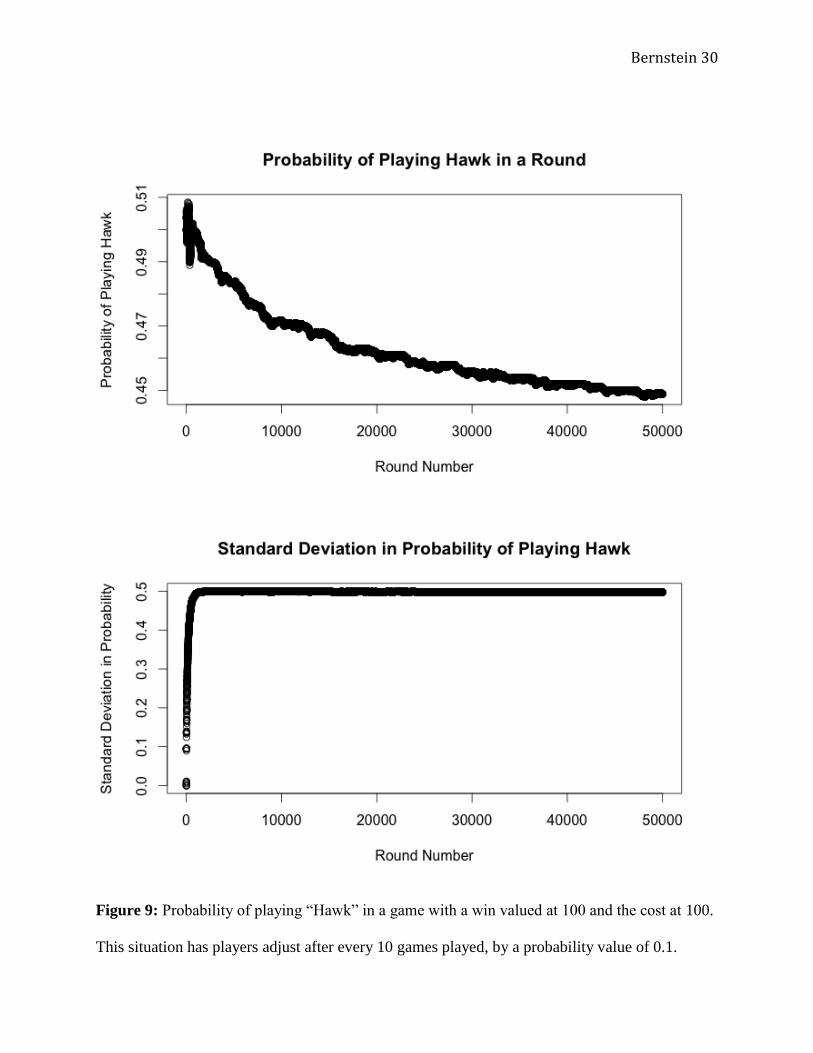
I also tested a probability adjustment of 0.1 (Figure 9). In general, I expected to see

similar results as the prior two, but “sped up” somewhat. This is exactly what happened. The

Bernstein 14

long-term probability of playing “Hawk” decreased even further, to 0.453 and the standard

deviations increased even faster than in Figure 7.

When the learning period was extended to 50 games for the prior three scenarios, the

results differed dramatically. Rather than a consistent downward pressure, the probability

adjustment values of 0.05 (Figure 10) and 0.1 (Figure 12) resulted in constant values, relatively

close to the steady state at 0.503 and 0.496 probability of playing “Hawk,” respectively. The

probability adjustment rate of 0.01(Figure 11) did not reach a constant, but appeared to alternate

around the long-term mean value of 0.503 probability of playing “Hawk.” The standard

deviations increased quickly then leveled off for adjustment values of 0.05 and 0.1, but seemed

to increase throughout all 50,000 games for the adjustment value of 0.01. This may be due to the

fact that the scenario was simply not long enough, and that the players simply hadn’t reached a

constant value. This is supported in the examination of the other two situations: with a

probability adjustment value of 0.1, the aggregate probability seemed to reach a constant value

after the first 10,000 or so games. With the probability adjustment value of 0.05, it took almost

40,000 games to each the steady state constant value.

6. Conclusion

Although the simulated results for mixed strategies were close, they didn’t converge

exactly to the correct values. Interestingly, for the intermediate situations (Figures 5 and 6), and

similarly visible in the situations when V was valued at 100 and C at 100 (Figure 1) or 50 (Figure

2), the divergence in the values seems to follow a pattern. The situations that have a theoretical

ESS closer to a 0.5 probability of playing “Hawk” resulted in a convergence closer to the

Bernstein 15

expected values. This seems to suggest that this model is somewhat biased towards intermediate

values, pushing each player’s likelihood of playing “Hawk” or “Dove” away from a pure

strategy ESS and closer to a 0.5 chance of either occurring. This may be due to the fact that all

players start with an equal probability of playing either strategy, or because the “edge cases”7 I

created push players away from a pure strategy in most situations.

The exception to this seemed to be when the ESS was to play “Hawk” and “Dove” with

even probability. Over a very long period of time, with a relatively short learning memory, the

results suggest that the average likelihood to play “Hawk” decreases slightly over the very long-

term. This phenomenon may be due to the fact that a random number generator was used, but its

consistent appearance across three simulations suggests that it is likely a quirk in how I

programmed my model. Interestingly, the opposite happened when both the learning rate was

decreased and the period learned from was extended, albeit the effect was much smaller.

Taking the above into account, the model I created generates results that are

reasonably close to the predicted ESS values and simply altering the parameters behind the

learning algorithm can increase the accuracy by orders of magnitude. In fact, the variation

from predicted values should be expected largely because of the random matching of players.

While the algorithm I used differed slightly from more commonly understood learning methods,

the similarity to the predicted ESS suggests that this approach, while imperfect, is still useful for

understanding how evolutionary dynamics occur over time.

Interestingly, the parameter that had the largest impact on the “accuracy” of the model,

relative to the predicted ESS, was the number of games over which an individual player learned.

7 The “edge cases” described involve what happens when a pure strategy is played, i.e. if or . In these cases, the model verifies that the player could not obtain a higher score. If , then an agent plays only “Dove.” If the entire population follows this strategy, then an individual can earn more by deviating to play “Hawk” by even the slightest amount. Therefore, the model checks to see

if

, before it allows . If for a player, the model checks to see if that player is earning the lowest possible score. If

he is, then, because he should be either indifferent or seek to deviate from his current strategy, the model decreases his likelihood to play “Hawk” in the future, therefore reintroducing the “Dove” strategy.

Bernstein 16

Increasing this number led to results significantly closer to the predicted ESS. I believe this

result is more accurate because it allows each player a much better understanding of the

population it plays against.

When I examined the rate of convergence to the steady state in each situation, I noticed

that the probability adjustment value had the most dramatic effect. The larger the value, the

faster the results seemed to converge to a steady state of sorts. This is evident from Figures 10,

11, and 12: The results in Figure 12, with the largest adjustment value, converged in about

10,000 games. The results in Figure 10, with the middle adjustment value, converged after

nearly 40,000 games, while the results in Figure 11 never quite reached a constant value.

Similarly, when each player was limited to learning from only the prior 10 games, after 50,000

games, none of the games with and reached a constant average. Beyond

exploring in a more in-depth fashion how the learning period affects the variation from the

predicted ESS, further studies with this type of approach can both extend the scenario

significantly and alter the size of the population. Beyond examination of the Hawk-Dove game,

this type of methodology can also be applied to other games, such as the Repeated Prisoner’s

Dilemma or the Dictator or Ultimatum games in order to understand how evolutionary and

learning dynamics occur in other situations, and to compare a computer simulation of learning to

behavioral studies.

Bernstein 17

References

Borgers, T, and Rajiv Sarin. "Learning Through Reinforcement and Replicator Dynamics*1,

*2." Journal of Economic Theory 77.1 (1997): 1-14. ScienceDirect. Web. 28 Nov. 2013.

Friedman, Daniel. "On Economic Applications of Evolutionary Game Theory." Journal

of Evolutionary Economics 8.1 (1998): 15-43. Web. 23 Feb. 2014.

Fudenberg, Drew, and David K. Levine. The Theory of Learning in Games. Cambridge, MA:

MIT, 1998. Print.

Gaunersdorfer, Andrea, and Josef Hofbauer. "Fictitious Play, Shapley Polygons, and the

Replicator Equation." Games and Economic Behavior 11.2 (1995): 279-303. Web. 21

Jan. 2014.

Matsumura, Shuichi. "The Evolution of “egalitarian” and “despotic” Social Systems among

Macaques." Primates Socioecology 40.1 (1999): 23-31. ScienceDirect. Web. 28 Nov.

2013.

Mcadams, Richard H., and Janice Nadler. "Testing the Focal Point Theory of Legal

Compliance: The Effect of Third-Party Expression in an Experimental Hawk/Dove

Game." Journal of Empirical Legal Studies 2.1 (2005): 87-123. Web. 22 Feb. 2014.

Neugebauer, Tibor, Anders Poulsen, and Arthur Schram. "Fairness and Reciprocity in the

Hawk–Dove Game." Journal of Economic Behavior & Organization 66.2 (2008): 243-

50. ScienceDirect. 31 Oct. 2006. Web. 28 Nov. 2013.

Orzack, Steven Hecht, and W. G. S. Hines. "The Evolution Of Strategy Variation: Will An ESS

Evolve?" Evolution 59.6 (2005): 1183-193. Web. 3 Mar. 2014.

Bernstein 18

Pettitt, A. N. "Testing the Normality of Several Independent Samples Using the Anderson-

Darling Statistic." Journal of the Royal Statistical Society C 26.2 (1977): 151-61. JSTOR.

Web. 1 Dec. 2013.

Samuelson, Larry. "Evolution and Game Theory." Journal of Economic Perspectives 16.2

(2002): 47-66. JSTOR. Web. 28 Nov. 2013.

Smith, J. Maynard. "The Theory of Games and the Evolution of Animal Conflicts." Journal of

Theoretical Biology 47.1 (1974): 209-21. Web. 2 Mar. 2014.

Strogatz, Steven H. Nonlinear Dynamics and Chaos: With Applications to Physics, Biology,

Chemistry, and Engineering. Reading, MA: Addison-Wesley Pub., 1994. Print.

Bernstein 19

Appendices

Appendix A: Figures and Tables

Hawk Dove

Hawk

Dove

Table 1: Payoff Matrix for the Hawk-Dove Game

V is a fixed win amount; C is a fixed cost amount.

(Samuelson, 2002)

Simulation

(Appendix

Figure)

Win

(V) Cost (C)

Predicted

PH

Mean PH

(Final 50% of Games) Lower CI- 5% Upper CI- 5%

1 100 100 0.500 0.495 0.495 0.495

2 100 50 * 0.891 0.891 0.891

3 0 100 0.000 0.005 0.005 0.005

4 100 49 1.000 1.000 1.000 1.000

Table 2: Initial Scenarios— Initial ESS Monte Carlo Simulations

Adjustment value of 0.05

Predicted PH = (V/2) – C

Mean PH is the average value of the simulated PH in the final 5000 rounds of play

CI is the confidence interval

* Nash Equilibrium, not ESS

Bernstein 20

Simulation

(Appendix

Figure)

Win

(V) Cost (C)

Predicted

PH

Mean PH


5 100 60 0.833 0.767 0.767 0.767

6 100 200 0.250 0.283 0.283 0.283

Table 3: Secondary Scenarios— Intermediate mixed-strategy ESS Monte Carlo

Simulations

Adjustment Value of 0.05

Predicted PH = (V/2) – C

Mean PH is the average value of the simulated PH in the final 5000 rounds of play

CI is the confidence interval

Win (V) Cost (C)

Learning

Period

(# of Games)

Predicted

PH

Mean PH


0 100 50 0 0.034 0.034 0.034

100 100 5 0.500 0.462 0.462 0.462

100 100 50 0.500 0.499 0. 499 0. 499

100 50 50 * 0.977 0.977 0. 977

100 60 50 0.833 0.806 0.806 0.806

100 200 50 0.250 0.273 0.273 0.273

Table 4: Robustness Tests— ESS and Monte Carlo Simulations Adjustment Value of 0.05 Predicted PH = (V/2) – C Mean PH is the average value of the simulated PH in the final 5000 rounds of play CI is the confidence interval * indicates that the game involves a Nash Equilibrium, but not an ESS

Bernstein 21

Simulation

(Appendix

Figure)

Adjustment

Value

Learning

Period

(# of

Games)

Predicted

PH

Mean PH

(Final 50% of

Games)

Lower CI- 5% Upper CI- 5%

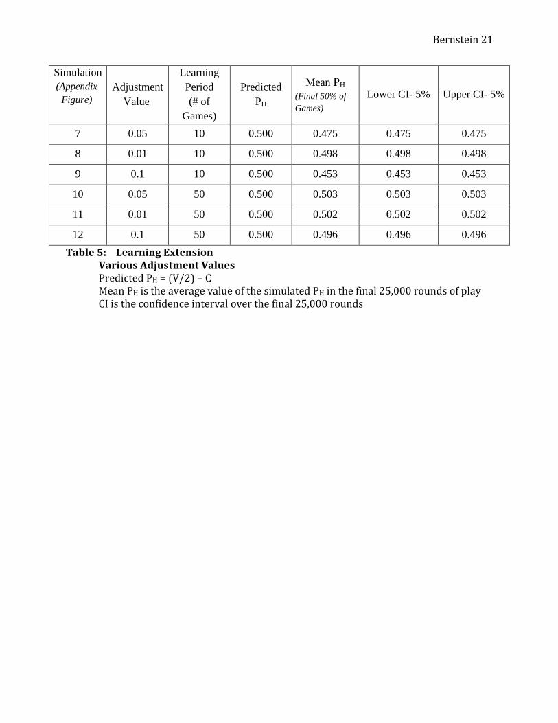
7 0.05 10 0.500 0.475 0.475 0.475

8 0.01 10 0.500 0.498 0.498 0.498

9 0.1 10 0.500 0.453 0.453 0.453

10 0.05 50 0.500 0.503 0.503 0.503

11 0.01 50 0.500 0.502 0.502 0.502

12 0.1 50 0.500 0.496 0.496 0.496

Table 5: Learning Extension Various Adjustment Values Predicted PH = (V/2) – C Mean PH is the average value of the simulated PH in the final 25,000 rounds of play CI is the confidence interval over the final 25,000 rounds

Bernstein 22

Figure 1: Probability of playing “Hawk” in a game with a win valued at 100 and the cost at 100.

This situation has players adjust after every 10 games played by a probability value of 0.05.

Bernstein 23


This situation has players adjust after every 10 games played.

Bernstein 24



Bernstein 25



Bernstein 26



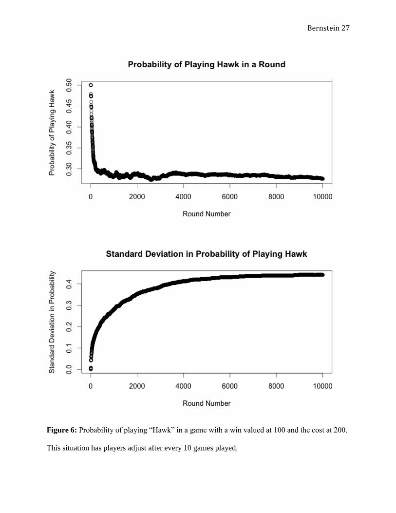
Bernstein 27



Bernstein 28


This situation has players adjust after every 10 games played, by a probability value of 0.05.

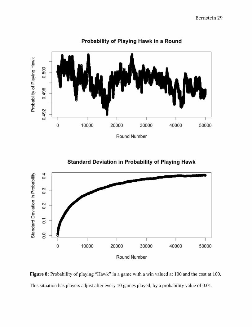
Bernstein 29



Bernstein 30



Bernstein 31

Figure 10: Probability of playing “Hawk” in a game with a win valued at 100 and the cost at

100. This situation has players adjust after every 50 games played, by a probability value of

0.05.

Bernstein 32


100. This situation has players adjust after every 50 games played, by a probability value of

0.01.

Bernstein 33


100. This situation has players adjust after every 50 games played, by a probability value of 0.1.

Bernstein 34

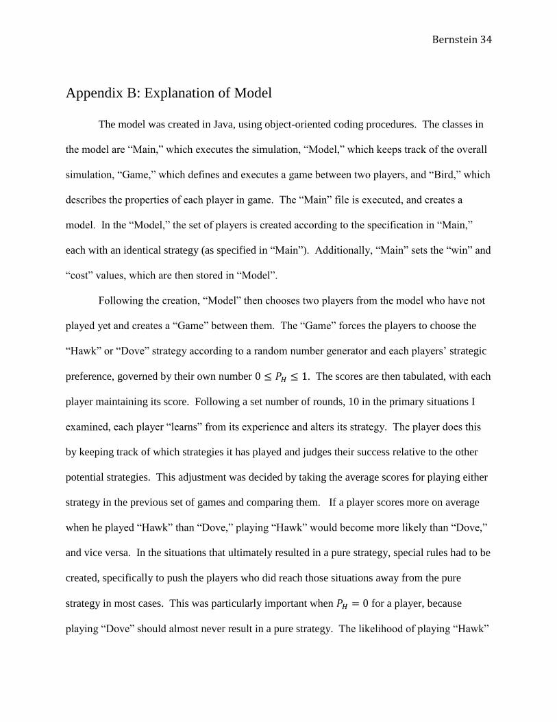
Appendix B: Explanation of Model

The model was created in Java, using object-oriented coding procedures. The classes in

the model are “Main,” which executes the simulation, “Model,” which keeps track of the overall

simulation, “Game,” which defines and executes a game between two players, and “Bird,” which

describes the properties of each player in game. The “Main” file is executed, and creates a

model. In the “Model,” the set of players is created according to the specification in “Main,”

each with an identical strategy (as specified in “Main”). Additionally, “Main” sets the “win” and

“cost” values, which are then stored in “Model”.

Following the creation, “Model” then chooses two players from the model who have not

played yet and creates a “Game” between them. The “Game” forces the players to choose the

“Hawk” or “Dove” strategy according to a random number generator and each players’ strategic

preference, governed by their own number . The scores are then tabulated, with each

player maintaining its score. Following a set number of rounds, 10 in the primary situations I

examined, each player “learns” from its experience and alters its strategy. The player does this

by keeping track of which strategies it has played and judges their success relative to the other

potential strategies. This adjustment was decided by taking the average scores for playing either

strategy in the previous set of games and comparing them. If a player scores more on average

when he played “Hawk” than “Dove,” playing “Hawk” would become more likely than “Dove,”

and vice versa. In the situations that ultimately resulted in a pure strategy, special rules had to be

created, specifically to push the players who did reach those situations away from the pure

strategy in most cases. This was particularly important when for a player, because

playing “Dove” should almost never result in a pure strategy. The likelihood of playing “Hawk”

Bernstein 35

was therefore adjusted upward in every case except for when

. This logically

follows because if the population uniformly plays “Dove,” and then any player that mutates to

play “Hawk” will score certainly higher unless . In the case that “Hawk” became a pure

strategy, the algorithm simply checked to see if the agent had received the lowest possible score

in each round. If it had, then its likelihood of playing “Hawk” decreased in the following round.

This process is then repeated within each round for all players until there are less than 2 players

left that have not played in the current round. Given that each simulation is limited to 1000

players for consistency, this should always result in each player playing a single game before any

player plays a second time. The entire process is then repeated as many times as were specified

in the model.

Bernstein 36

Appendix C: Numerical Example

Let , , games 650-660

Player 451 has a ; played “Hawk” 5 times (randomly selected from probability)

“t” refers to the 65th

set of games

Total Score over ten games against ten randomly selected opponents: 150

Total Score from playing Hawk: 100

Average “Hawk” Score:

, average

Average “Dove” Score:

, average

Because ,

Monte Carlo Simulation of Learning in the Hawk-Dove … Carlo Simulation of Learning in the Hawk ......

Documents

Transcript of Monte Carlo Simulation of Learning in the Hawk-Dove … Carlo Simulation of Learning in the Hawk ......