Monte Carlo Simulation of a Detector for Cosmic Rays

Monte Carlo Simulation of a Detector for Cosmic Rays

Bachelor Thesis of Pablo Sarazá Canflanca

Westfälische Wilhelms-Universität Münster Fachbereich Physik

- July 2014 –

Supervisor and first examiner: Privatdozent Dr. Christian Klein-Bösing Second examiner: Pr. Dr. Johannes P. Wessels Third examiner: Dr. Miguel Antonio Cortés Giraldo


1

Contents

1 Introduction 3

2 Theoretical Overview 4

2.1 Cosmic Rays….………………………………………………...…..…………… 4

2.1.1 Muons in Cosmic Rays…...………...…………………...……………… 5

2.2 Energy Loss of Charged Particles by Atomic Collisions…..……..…………….. 9

2.3 Geant4….………………………………………………...…..………...……… 11

3 Detector Set Up 13

4 Verification 17

4.1 Angular Distribution…………………………………………...…..……..…… 17

4.2 Lifetime of the Muons….……………………………………..…..…………… 18

4.3 Lifetime and Michel Triggers….……………………………………………... 19

4.4 MIP-Trigger…………………....……………………………………………… 20

5 Results of the simulation of a detector for cosmic muons 23

5.1 Energy Loss of Muons traversing the Detector ………...……...…..……..…… 23

5.2 Angular Dependence for the Intensity of Muons ….……………………………26


2

5.3 Mean Lifetime of Muons …………………………………………………….. 33

5.4 Michel Spectrum ……………………………………………………………… 35

6 Outlook and Summary 38


3

1 Introduction The topic of this bachelor thesis is the analysis of the results obtained by running a Monte Carlo simulation of a detector for cosmic muons, more precisely the muon detector located in the building of the Institut für Kernphysik in the Westfälische Wilhelms-Universität Münster.

When primary cosmic rays enter the upper Earth atmosphere, they interact with gas molecules, creating new particles, among them pions. Charged pions decay rapidly, and thus after traveling a short distance, into muons. These muons can be detected at sea level, where some of their properties such as life time, angular distribution or energy loss can be studied [1].

The simulation will study these characteristics as well. By applying different triggers, results will vary from the ideal case, where almost all the information from the muons can be obtained, to the real case, where the results should be similar to the ones obtained when working with the real detector.

In order to supply the basic knowledge needed to understand this thesis, a theoretical overview will introduce some of the basic concepts concerning cosmic rays and muons, the passage of particles through matter and the program used in the simulation, Geant4.


4

2 Theoretical Overview 2.1 Cosmic Rays In this section and the subsection 2.1.1 a theoretical introduction on cosmic rays and muons is offered to the reader. References [1-4] were used.

Cosmic rays are made of high-energy particles which source is outside the Earth. The energy range of cosmic rays spans from low energetic particles with < 109 eV to particles with an energy higher than 1020 eV. Their energy maximum remains still unknown. Although their origin is still not clear, there are some potential candidates that are generally accepted as probable sources: active galactic nuclei, quasars and supernova explosions.

There are two main steps in the life of cosmic rays which fall upon our planet:

- Primary cosmic rays: these are the particles that reach the atmosphere. The atmosphere does not present a well defined end, but rather has an exponential density distribution. The height of the atmosphere is generally considered to be of 40 km. Primary cosmic rays are mainly composed of protons (≈ 85%), α particles (≈ 12%) and heavy nuclei, nuclei of elements with Z ≥ 3 (≈ 3%). There are also electrons ( < 1%), positrons (≈ 0.1%) and antiprotons, which are even rarer and are probably generated during the interaction of primordial cosmic rays with interstellar gas.

- Secondary cosmic rays: when primary cosmic rays reach the atmosphere,

they interact with the atomic nuclei of the gas molecules. These interactions lead to the creation of different particles, pions above all, but also nucleons, photons, electrons and heavy mesons. Charged pions have a mean lifetime of (2.6033 ± 0.0005) · 10-8s, while the mean lifetime of neutral pions has a value of (8.52 ± 0.18) · 10-17s. For the charged pions, the primary decay mode is into a muon and a muon antineutrino. This decay mode has a ratio of (99.98770 ± 0.00004) %, which means most pions decay into muons and other decay modes are negligible.

𝝅 → 𝝁 + 𝝂𝝁 (2.1)


5

𝝅 → 𝝁 + 𝝂𝝁 (2.2)

The principal decay mode of neutral pions is into two photons with a rate of (98.823 ± 0.034) %. The muons originated in the decay of charged pions are the ones that will be detected in the experiment.

2.1.1 Muons in cosmic rays Muons are leptons with a mean lifetime of (2.1969811 ± 0.0000022) μs and a mass of (105.6583715 ± 0.0000035) MeV/c2. They have the same electrical charge as the electron (or positron for the antimuon). The decay of muons is always mediated by the weak interaction. Muons (antimuons) decay into an electron (positron), an electron antineutrino (electron neutrino) and a muon neutrino (muon antineutrino). 𝝁 → 𝒆 + 𝝂𝒆 + 𝝂𝝁 (2.3) 𝝁 → 𝒆 + 𝝂𝒆 + 𝝂𝝁 (2.4) Now some of the main properties of the cosmic muons that are studied with the detector will be introduced:

- Energy distribution of the cosmic muons: the energy distribution of the cosmic muons that incise in the vertical direction is the one shown in Figure 1.


6

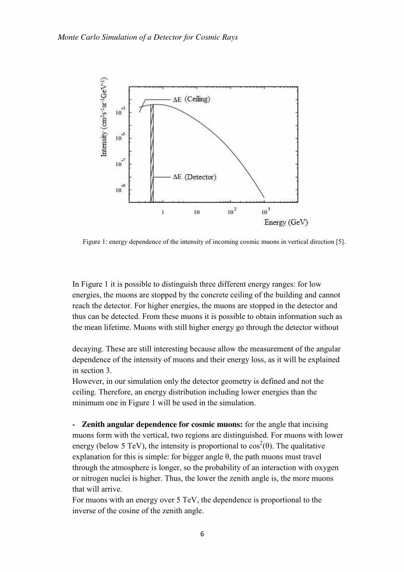
Figure 1: energy dependence of the intensity of incoming cosmic muons in vertical direction [5].

In Figure 1 it is possible to distinguish three different energy ranges: for low energies, the muons are stopped by the concrete ceiling of the building and cannot reach the detector. For higher energies, the muons are stopped in the detector and thus can be detected. From these muons it is possible to obtain information such as the mean lifetime. Muons with still higher energy go through the detector without decaying. These are still interesting because allow the measurement of the angular dependence of the intensity of muons and their energy loss, as it will be explained in section 3. However, in our simulation only the detector geometry is defined and not the ceiling. Therefore, an energy distribution including lower energies than the minimum one in Figure 1 will be used in the simulation.

- Zenith angular dependence for cosmic muons: for the angle that incising muons form with the vertical, two regions are distinguished. For muons with lower energy (below 5 TeV), the intensity is proportional to cos2(θ). The qualitative explanation for this is simple: for bigger angle θ, the path muons must travel through the atmosphere is longer, so the probability of an interaction with oxygen or nitrogen nuclei is higher. Thus, the lower the zenith angle is, the more muons that will arrive. For muons with an energy over 5 TeV, the dependence is proportional to the inverse of the cosine of the zenith angle.


7

For Eµμ < 5 TeV, 𝑰𝝁~ (𝐜𝐨𝐬𝜽)𝟐 (2.5) For Eµμ > 5 TeV, 𝑰𝝁~

𝟏𝐜𝐨𝐬 𝜽

(2.6)

However, the intensity of muons with an energy over 5 TeV is less than one millionth the intensity of muons with lower energies, so the simulation will not take it into account.

Figure 2: zenith angular dependence for muons with E < 5 TeV [3].

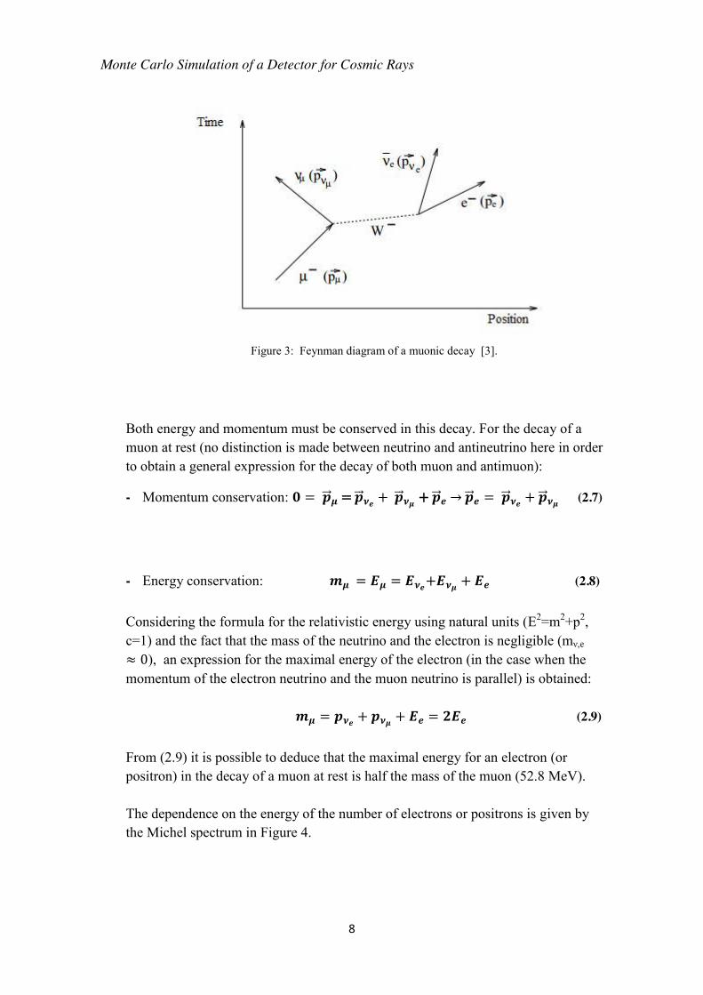
- Michel spectrum: the decay of a muon is mediated through the weak interaction and thus, through the exchange of a virtual boson W- or W+ for muon and antimuon. In the Figure 3, the decay of a muon is presented.


8

Both energy and momentum must be conserved in this decay. For the decay of a muon at rest (no distinction is made between neutrino and antineutrino here in order to obtain a general expression for the decay of both muon and antimuon):

- Momentum conservation: 𝟎 = �⃗�𝝁 = �⃗�𝝂𝒆 + �⃗�𝝂𝝁 + �⃗�𝒆 → �⃗�𝒆 = �⃗�𝝂𝒆 + �⃗�𝝂𝝁 (2.7)

- Energy conservation: 𝒎𝝁 = 𝑬𝝁 = 𝑬𝝂𝒆+𝑬𝝂𝝁 + 𝑬𝒆 (2.8)

Considering the formula for the relativistic energy using natural units (E2=m2+p2, c=1) and the fact that the mass of the neutrino and the electron is negligible (mν,e

≈ 0), an expression for the maximal energy of the electron (in the case when the momentum of the electron neutrino and the muon neutrino is parallel) is obtained:

𝒎𝝁 = 𝒑𝝂𝒆 + 𝒑𝝂𝝁 + 𝑬𝒆 = 𝟐𝑬𝒆 (2.9)

From (2.9) it is possible to deduce that the maximal energy for an electron (or positron) in the decay of a muon at rest is half the mass of the muon (52.8 MeV).

The dependence on the energy of the number of electrons or positrons is given by the Michel spectrum in Figure 4.

Figure 3: Feynman diagram of a muonic decay [3].


9

Figure 4: Michel spectrum. Energy of the electrons originated in a muonic decay [6].

2.2 Energy Loss of Charged Particles by Atomic Collisions When a charged particle travels through matter, it can lose energy and change its initial direction due to different processes which can occur. The main processes are inelastic collisions with the atomic electrons of the atoms of the material, elastic scattering with the nuclei, emission of Cherenkov radiation, nuclear reactions and bremstrahlung. However the most common ones are the elastic and inelastic scattering of the particles with the nuclei or the atomic electrons. The largest part of the energy loss corresponds then to the inelastic collisions with electrons. These are statistical in nature, but since their number in a macroscopic path length is usually large, it is possible to consider and work with an average energy loss per unit of path length traveled by the particle. Different calculations were made to obtain this mean energy, being the first correct quantum-mechanical one developed by Bethe, Bloch and other authors. The formula that calculates this value is known as the Bethe-Bloch formula. More precise information about it can be found in [7]. This formula leads to a dependence of the


10

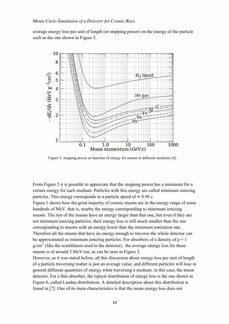
average energy loss per unit of length (or stopping power) on the energy of the particle such as the one shown in Figure 5.

From Figure 5 it is possible to appreciate that the stopping power has a minimum for a certain energy for each medium. Particles with this energy are called minimum ionizing particles. This energy corresponds to a particle speed of ≈ 0.96 c. Figure 1 shows how the great majority of cosmic muons are in the energy range of some hundreds of MeV, that is, nearby the energy corresponding to minimum ionizing muons. The rest of the muons have an energy larger than that one, but even if they are not minimum ionizing particles, their energy loss is still much smaller than the one corresponding to muons with an energy lower than the minimum ionization one. Therefore all the muons that have an energy enough to traverse the whole detector can be approximated as minimum ionizing particles. For absorbers of a density of ρ = 1 g/cm3 (like the scintillators used in the detector), the average energy loss for these muons is of around 2 MeV/cm, as can be seen in Figure 5. However, as it was stated before, all this discussion about energy loss per unit of length of a particle traversing matter is just an average value, and different particles will lose in general different quantities of energy when traversing a medium, in this case, the muon detector. For a thin absorber, the typical distribution of energy loss is the one shown in Figure 6, called Landau distribution. A detailed description about this distribution is found in [7]. One of its main characteristics is that the mean energy loss does not

Figure 5: stopping power as function of energy for muons in different mediums [4].


11

correspond to the most probable energy loss. This is due to the asymmetry of the distribution created by the long high energy tail. This tail is caused by the possibility of the particles to suffer a large energy transfer in a single collision.

2.3 Geant4

In this section, information found in [8] and [9] was used to comment some of the characteristics, applications and operation principles of Geant4. Geant4 is a toolkit for the simulation of the passage of particles through matter by using Monte Carlo methods, which involve the generation of random numbers in order to get numerical results from them. It was developed by CERN, and it uses object oriented programming in C++.

The widespread use of this software includes areas such as high energy physics (where it is used in BaBar at SLAC and ATLAS and CMS in CERN, among others), nuclear physics, space applications, research on technology transfer and works in medical science.

Figure 6: typical distribution of energy loss for particles traversing a thin absorber [7].


12

Geant4 enables definition of a detector and the generation and subsequent tracking of particles through that detector, which allows the study of the interaction between. It permits the collection of varied data such as the path traveled by a particle, its momentum or energy at a given point or, in case of occurring, its decay. Geant4 also enables the visualization of the simulation. Now it will be introduced a simple notion of Geant4 that will result useful later to understand how the information of the particles was obtained. During the flight of a particle, we distinguish two different types of elements in its path: steps and step-points. During a step, the particle travels between two points, its corresponding step- points. From each step and its corresponding two points (previous and posterior) diverse information such as name or mass of the particle, kinetic energy, position, momentum direction or energy deposited in that step can be extracted.


13

3 Detector Set Up In this section, the construction and operation of the cosmic ray detector is described. To this purpose [3], [7] and [10] were used.

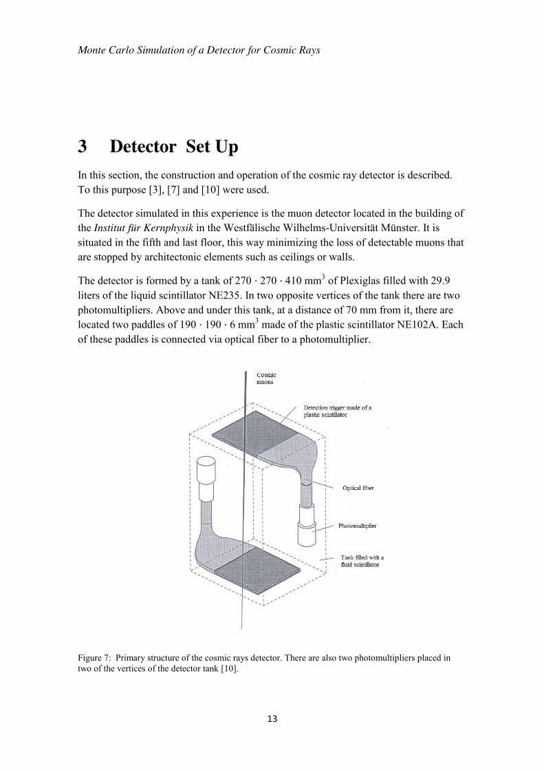
The detector simulated in this experience is the muon detector located in the building of the Institut für Kernphysik in the Westfälische Wilhelms-Universität Münster. It is situated in the fifth and last floor, this way minimizing the loss of detectable muons that are stopped by architectonic elements such as ceilings or walls.

The detector is formed by a tank of 270 · 270 · 410 mm3 of Plexiglas filled with 29.9 liters of the liquid scintillator NE235. In two opposite vertices of the tank there are two photomultipliers. Above and under this tank, at a distance of 70 mm from it, there are located two paddles of 190 · 190 · 6 mm3 made of the plastic scintillator NE102A. Each of these paddles is connected via optical fiber to a photomultiplier.

Figure 7: Primary structure of the cosmic rays detector. There are also two photomultipliers placed in two of the vertices of the detector tank [10].


14

Some of the main properties of the scintillator materials in the detector are presented in table 1.

Scin-

tillator Type Density

(g/cm3) Refractive

Index Decay time max. com- ponent (ns)

Wave- length of emission

(nm)

H/C ratio

Light output

NE102A Plastic 1.032 1.581 2.4 423 1.104 65 NE235 Liquid 0.858 1.47 4 420 2.0 40

Table 1: main properties of scintillators present in the detector [7].

In order to record the data, some output signals known as triggers are needed. There triggers are employed in the simulation to provide more realistic data and results. They involve some electronic devices and processes, but here they will be presented in a more qualitative way:

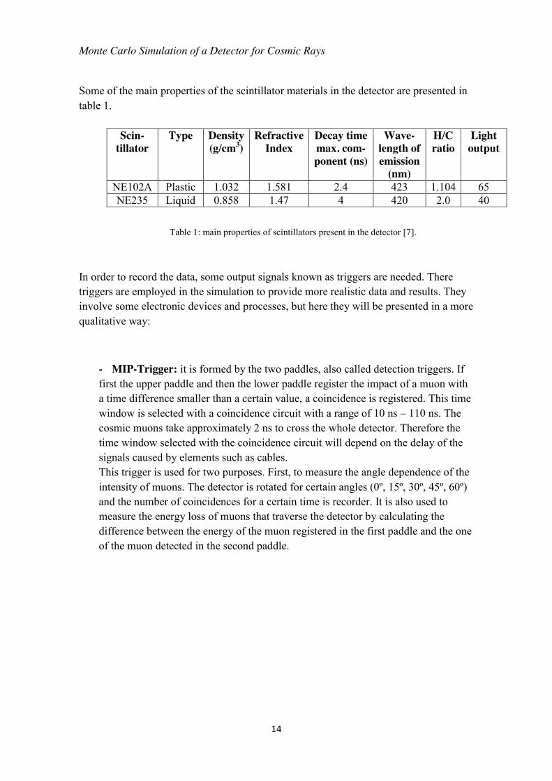
- MIP-Trigger: it is formed by the two paddles, also called detection triggers. If first the upper paddle and then the lower paddle register the impact of a muon with a time difference smaller than a certain value, a coincidence is registered. This time window is selected with a coincidence circuit with a range of 10 ns – 110 ns. The cosmic muons take approximately 2 ns to cross the whole detector. Therefore the time window selected with the coincidence circuit will depend on the delay of the signals caused by elements such as cables. This trigger is used for two purposes. First, to measure the angle dependence of the intensity of muons. The detector is rotated for certain angles (0º, 15º, 30º, 45º, 60º) and the number of coincidences for a certain time is recorder. It is also used to measure the energy loss of muons that traverse the detector by calculating the difference between the energy of the muon registered in the first paddle and the one of the muon detected in the second paddle.


15

- Lifetime trigger: this trigger is activated for the muons that decay, which are around 1% of the total that will reach the detector. The flux of muons is 200 per square meter and second. Since the detector has an upper surface of 270 x 270 mm2, this means that on average 15 muons will reach the detector every second. This means a muon on average every 0.0686 s. From there it can be deduced that if in an interval of 20 μs after a muon is detected an electron is detected, there is a probability of 99.97 % that electron is originated in the decay of that muon [3]. Therefore the muon-electron signals separated by a time smaller than 20 μs are selected. From the exponential decay law and the fact that the mean lifetime of muons is 2.2 μs, it follows that 99.99 % of the muons decay in an interval of 20 μs. By measuring the time difference between the signal of the stopped muons and the signal of the corresponding electrons, the mean lifetime is obtained.

- Michel trigger: the working principle is very similar to the one of the lifetime trigger. The Michel spectrum is the energy spectrum of the electrons (or positrons) originated in a muon (or antimuon) decay. Therefore, to ensure that the electron signal registered stems from an electron created in the decay of a muon, only

Figure 8: MIP-Trigger. The dotted arrow represents a particle that does not activate the trigger. The continuous arrow one that does activate it [3].


16

signals from electrons registered in an interval of 10 μs after the signal of a muon are accepted. The interval is smaller than the one of the lifetime trigger to minimize the probability of non-correspondence between the muon and electron signals.


17

4 Verification In this section the results of the running of different simulations will be presented. These simulations do not correspond to the real case, but rather are useful to verify that some of the parameters such as angular distribution, some values such as lifetime or some triggers such as the MIP-trigger are currently implemented.

This way some undesired mistakes of diverse nature can be detected and subsequently corrected. In our case, for example, a mean muon lifetime of the order of nanoseconds was obtained, when in reality it is of the order of microseconds. This was caused by a bad choice of the “Physics List” (we were working with the Physics List QBBC provided by Geant4), the file that contain the physical information concerning interaction and decay of particles.

4.1 Angular Distribution This simulation consists of 25000 monoenergetic (10 MeV) muons shot upon a prism shaped detector of organic liquid (C18H14) of 20·20·30 cm3 from a distance of 2 cm. To obtain the angular distribution, the mechanism used in the real detector was not used, but rather a more accurate way allowed by the Geant4 software. The momentum direction of each muon was registered the moment it entered our detector. This was performed by the command G4StepPoint::GetMomentumDirection() for the first point of each particle inside the detector.Therefore only the momentum direction of the particles that entered the detector (in this case 24994 out of 25000) was registered.


18

Figure 9: verification of the angular distribution by fitting with a cos2(θ) function.

From Figure 7 it is possible to appreciate that the zenith angular distribution of the muons is indeed cos2(θ).

4.2 Lifetime of the Muons The verification of the mean lifetime of the muons has two main purposes: first of all it is useful to check that the commands used to obtain this data is the correct one, that is, that the time being measured corresponds to the moment when the muon decays and not to some other event. Second of all it is useful to check that the “Physics List” used is the appropriate one. This can be a problem because there are several lists available, each suitable for the study of a certain field, and the use of the wrong list can lead to mistaken results such as a wrong value for the mean lifetime of muons.

In this case the run was the same as in section 4.1. It consisted of 25000 monoenergetic (10 MeV) muons shot upon a prism of organic liquid C18H14. The conditions used to define the point at which the decay time is registered are the following. The particle tracked must be a muon, it must decay during a certain step and at the point previous to


19

that step it must be inside the prism detector. The time at that step is registered by using the command G4Track::GetGlobalTime() on that step. This way only the lifetime of the particles that decay inside the detector is recorded, which makes this calculation more realistic.

Figure 10: verification of the mean lifetime of muons.

A lifetime of (2.200 ± 0.014) μs is obtained. This agrees with the expected theoretical value in [4].

4.3 Lifetime and Michel Trigger For the measurement of both the mean lifetime and the Michel spectrum, only the muons that decay inside the tank of the detector can be detected in the real experiment. To check that this is also fulfilled in the simulation, a three dimensional histogram that displays the decay position of the muons is developed. The axis are such that the histogram represents only the volume corresponding to the detector tank.


22

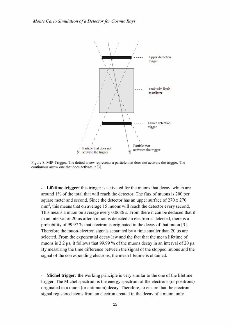
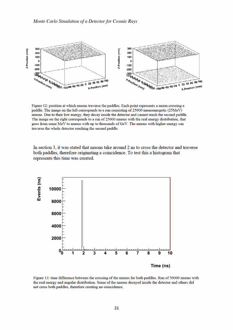
In Figure 13 all the times are between 1 ns and 3 ns, not even approaching 10 ns. The average time for muons to traverse the whole detector (for muons that cross both paddles) is

𝑡 = 1.864 ± 0.001 𝑛𝑠

This demonstrates that the time selected by the coincidence circuit (between 10 ns and 110 ns) corresponds mainly to the delay caused by the electronic components of our detector, and not to the real time needed by the muons to cross the device.


23

5 Results of the simulation of a detector for cosmic muons In this section the results obtained in the simulation of the measurements carried out in the real detector will be presented. Unlike in section 4, these results will be obtained using methods that imitate the triggers and limitations of the real detector. It will be discussed how the implementation of these triggers affects the results obtained and their accordance or discrepancy with the real values.

In order to obtain realistic measurements, the conditions for each simulation must be the ones under which the real detector is operating. However, when measuring a certain quantity, it may occur that only some of the muons have interest. For example, when measuring the mean lifetime of muons, only those which energy is low enough to allow them to decay inside the detector will contribute to the measurement. Since they correspond to a small part of the whole spectrum, a much longer time would be needed for this simulation to be executed if the whole spectrum of muons was considerer. By working with a simulation with muons of sufficiently low energy , the simulation time is substantially reduced without altering the results. Thus each result will be accompanied by a description and an explanation of the conditions under which the simulation was run.

5.1 Energy Loss of Muons traversing the Detector As it was stated before, in order to measure the energy loss of the muons, the MIP-Trigger must be activated. This means only the energy loss for muons that traverse both paddles in less than 10 ns will be registered. The value saved will be the difference between the energies measured at both paddles.

To obtain the energy of a muon when it crosses one of the paddles, the following method is used. First of all we impose that the particle is a muon and that the current step of its trajectory is inside the volume of the corresponding paddle. These conditions are implemented with the commands G4ParticleDefinition::GetParticleMass() and G4VPhysicalVolume::GetName(). The time at which it crosses the paddle is obtained by the command G4Track::GetGlobalTime(). It will later be used to impose the time condition of the MIP-Trigger in the root histogram file. The energy of the muon at the paddle is obtained with G4StepPoint::GetKineticEnergy().


25

Keeping the geometry of the detector in mind, there is a range of path lengths that each muon can travel. In the case where the incident muon has a zenith angle θ = 0º, it would travel the shortest way through the detector traversing 0.6 cm of the first paddle, then 41 cm of the tank and then 0.6 cm of the second paddle, making a total of 1.2 cm through the plastic scintillator and 41 cm through the liquid scintillator, 42.2 cm in total.

The longest possible path corresponds to muons that enter the detector and traverse both paddle in opposite vertices (Figure 15). That would correspond to muons with a zenith angle of 25.8º traveling 0.67 in each paddle and 45.5 cm in the liquid scintillator for a total of 46.8 cm.

For the mean stopping power of 2.3 MeV/cm discussed before, the mean energy loss of 100.6 MeV would result in a mean traveled distance of 43.8 cm. This is a value that fits between the possible minimum and maximum distances that a muon can travel in order to activate the MIP-Trigger and confirms our theoretically expected value.

In the real detector, the energy loss of the muons is stored in channels, but the real energy value of that loss is not obtained. Using this simulation the relation channel-energy can be established allowing to calibrate the experimental device.

Figure 15: longest and shortest possible paths for muons activating the MIP-Trigger.


26

5.2 Angular Dependence for the Intensity of Muons For this measurement, the number of coincidences, that is, of muons that traverse both paddles in less than 10 ns, will be registered for different angles of rotation for the detector (15º, 30º and 45º).

The total energy and angular distributions will be used for the muons. The same source will be used for each case because it is important that each simulation is working under the same conditions. This source will be close enough with the detector and large enough to assure that muons can fall upon the detector with all possible angles that would fulfill the MIP-Trigger condition. However it has to be a certain distance away from the detector so that they do not collide when the detector is rotated. Since for each angle the number of muons registered may be different, the number of muons shot may vary for each simulation, since the important quantity is the percentage of recorded muons, not the absolute value.

Now the results obtained are presented. The histograms corresponding to the energy loss are presented. The important value is the number of entries, that represents the number of coincidences in both paddles.


27

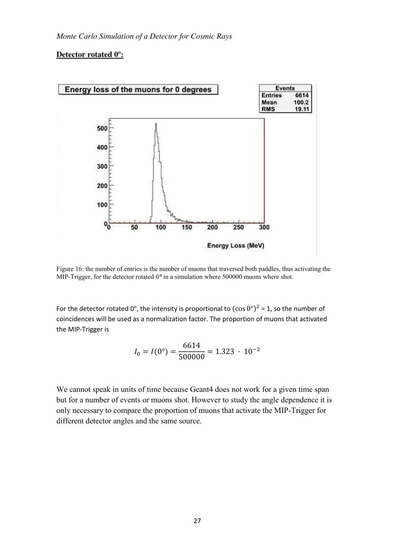
Detector rotated 0º:

Figure 16: the number of entries is the number of muons that traversed both paddles, thus activating the MIP-Trigger, for the detector rotated 0° in a simulation where 500000 muons where shot.

For the detector rotated 0°, the intensity is proportional to (cos 0°) = 1, so the number of

coincidences will be used as a normalization factor. The proportion of muons that activated

the MIP-Trigger is

𝐼 = 𝐼(0°) =6614500000

= 1.323 · 10

We cannot speak in units of time because Geant4 does not work for a given time span but for a number of events or muons shot. However to study the angle dependence it is only necessary to compare the proportion of muons that activate the MIP-Trigger for different detector angles and the same source.


28


Figure 17: muons that activated the MIP-Trigger for a run with 1000000 muons and the detector rotated 𝟏𝟓°.

𝐼(15°) =688510

= 6.885 · 10 = 0.520 𝐼

The theoretically expected intensity for a zenith angle of 15º is

𝐼 (15°) = (cos 15°) · 𝐼 = 0.933 𝐼

It is possible to define a parameter equivalent to the efficiency for the detector at each angle. For 15º, the efficiency of the detector is

𝜂 ° = 0.520𝐼0.933𝐼

= 0.557

This discrepancy will be discussed later together with the one of following results.


29


Figure 18: muons that activated the MIP-Trigger for a run with 1250000 muons and the detector rotated 𝟑𝟎°.

𝐼(30°) =3341

1.25 · 10= 2.673 · 10 = 0.202 𝐼


𝐼 (30°) = (cos 30°) · 𝐼 = 0.750 𝐼

For 45º, the efficiency of the detector is

𝜂 ° = 0.117𝐼0.500𝐼

= 0.269


30


Figure 19: muons that activated the MIP-Trigger for a run with 1500000 muons and the detector rotated 𝟒𝟓°.

𝐼(45°) =2320

1.5 · 10= 1.547 · 10 = 0.117 𝐼


𝐼 (45°) = (cos 45°) · 𝐼 = 0.500 𝐼

For 45º, the efficiency of the detector is

𝜂 ° = 0.117𝐼0.500𝐼

= 0.234

Plotting the obtained angular dependence together with the theoretically expected one, the following graph is obtained:


31

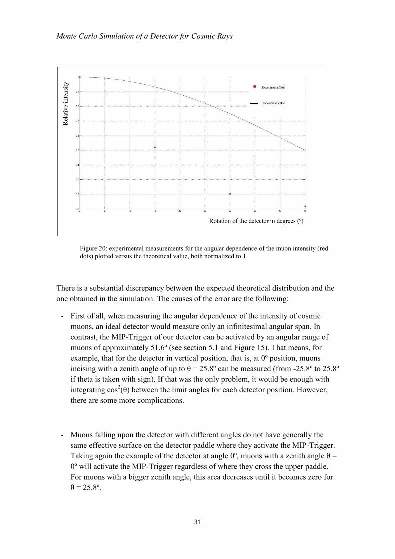
Figure 20: experimental measurements for the angular dependence of the muon intensity (red dots) plotted versus the theoretical value, both normalized to 1.

There is a substantial discrepancy between the expected theoretical distribution and the one obtained in the simulation. The causes of the error are the following:

- First of all, when measuring the angular dependence of the intensity of cosmic muons, an ideal detector would measure only an infinitesimal angular span. In contrast, the MIP-Trigger of our detector can be activated by an angular range of muons of approximately 51.6º (see section 5.1 and Figure 15). That means, for example, that for the detector in vertical position, that is, at 0º position, muons incising with a zenith angle of up to θ = 25.8º can be measured (from -25.8º to 25.8º if theta is taken with sign). If that was the only problem, it would be enough with integrating cos2(θ) between the limit angles for each detector position. However, there are some more complications.

- Muons falling upon the detector with different angles do not have generally the same effective surface on the detector paddle where they activate the MIP-Trigger. Taking again the example of the detector at angle 0º, muons with a zenith angle θ = 0º will activate the MIP-Trigger regardless of where they cross the upper paddle. For muons with a bigger zenith angle, this area decreases until it becomes zero for θ = 25.8º.


32

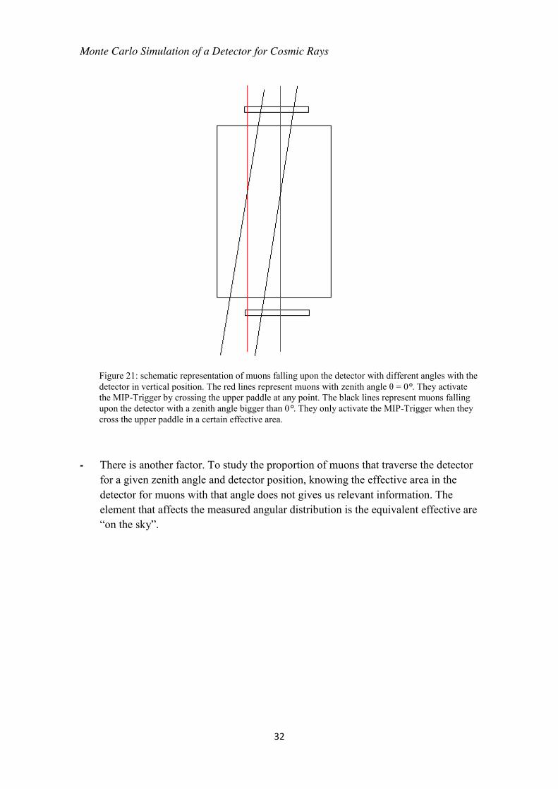
- There is another factor. To study the proportion of muons that traverse the detector for a given zenith angle and detector position, knowing the effective area in the detector for muons with that angle does not gives us relevant information. The element that affects the measured angular distribution is the equivalent effective are “on the sky”.

Figure 21: schematic representation of muons falling upon the detector with different angles with the detector in vertical position. The red lines represent muons with zenith angle θ = 0°. They activate the MIP-Trigger by crossing the upper paddle at any point. The black lines represent muons falling upon the detector with a zenith angle bigger than 0°. They only activate the MIP-Trigger when they cross the upper paddle in a certain effective area.


33

-

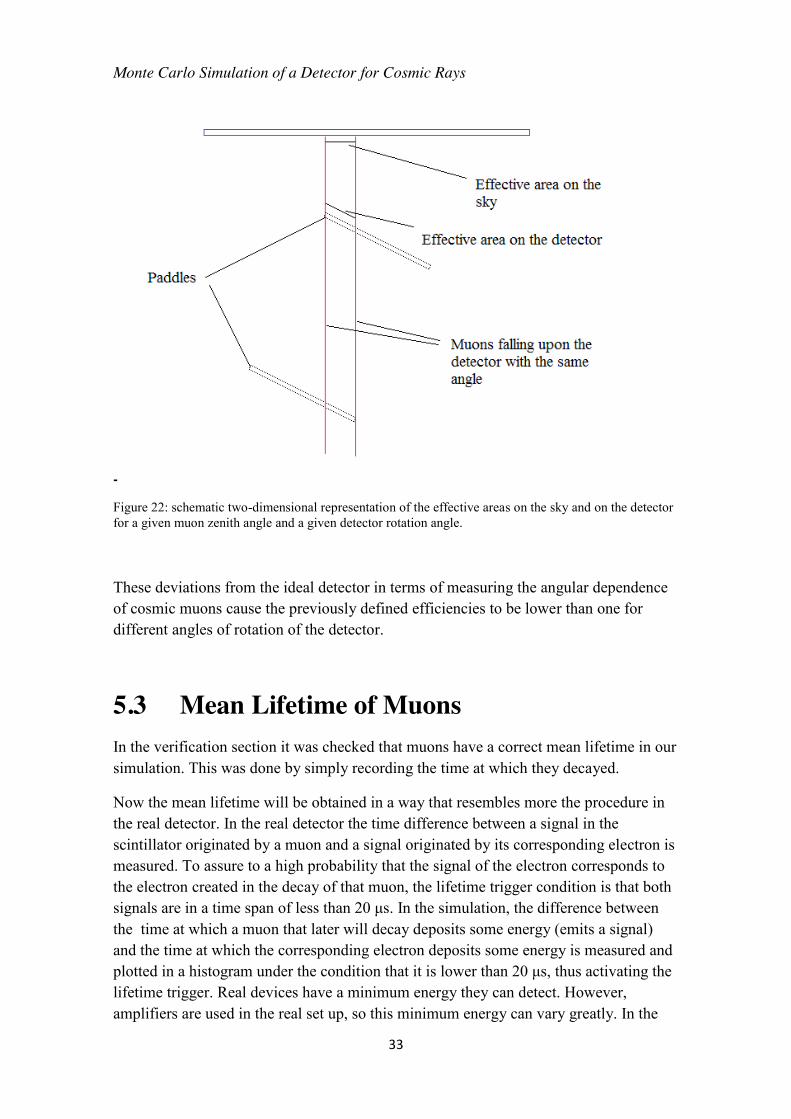
Figure 22: schematic two-dimensional representation of the effective areas on the sky and on the detector for a given muon zenith angle and a given detector rotation angle.

These deviations from the ideal detector in terms of measuring the angular dependence of cosmic muons cause the previously defined efficiencies to be lower than one for different angles of rotation of the detector.

5.3 Mean Lifetime of Muons In the verification section it was checked that muons have a correct mean lifetime in our simulation. This was done by simply recording the time at which they decayed.

Now the mean lifetime will be obtained in a way that resembles more the procedure in the real detector. In the real detector the time difference between a signal in the scintillator originated by a muon and a signal originated by its corresponding electron is measured. To assure to a high probability that the signal of the electron corresponds to the electron created in the decay of that muon, the lifetime trigger condition is that both signals are in a time span of less than 20 μs. In the simulation, the difference between the time at which a muon that later will decay deposits some energy (emits a signal) and the time at which the corresponding electron deposits some energy is measured and plotted in a histogram under the condition that it is lower than 20 μs, thus activating the lifetime trigger. Real devices have a minimum energy they can detect. However, amplifiers are used in the real set up, so this minimum energy can vary greatly. In the


34

code, a minimum deposited energy of 1 MeV has been chosen for both muons and electrons. When the energy deposited reaches that value, the time is recorded by means of the command G4Track::GetGlobalTime().

For this simulation, the normal angle distribution was used, but only muons with energy up to 100 MeV. Only muons with an energy lower than approximately 85 MeV decay in the detector. This corresponds to a small fraction of the spectrum, so if we worked with muons of every possible energy, the simulation would result too large and would take a long time without adding any interesting information about the lifetime of the decaying muons.

For a run of 750000 muons, these were the results obtained for the lifetime of muons:

Figure 20: lifetime of the muons measured by taking the time difference between the muon and the electron signal.

It is obtained a lifetime of

𝜏 = (2.217 ± 0.021)𝜇𝑠

This value agrees with the theoretical value of 𝜏 = (2.1969811 ± 0.0000022) μs that was introduced in the theoretical overview, which means that the method used in the real detector to measure the mean lifetime of muons is correct.

To check the proportion of muons that are not taken into account because of the trigger condition, another histogram was plotted with the lifetimes of the muons that decayed


35

whether they fulfilled the trigger condition (decaying within a time interval of 20 𝜇𝑠) or not.

Figure 21: Lifetime measurements for a run of 750000 muons without the lifetime trigger condition.

Only 4 out of 488785 muons were neglected due to the trigger condition, which means that only a fraction of around 10-5 of the muons decay outside the time span of 20 μs. The same lifetime with the corresponding error is obtained, so the measurement is not altered by this trigger condition.

5.4 Michel Spectrum As it was explained in the theoretical overview, Michel spectrum is the name given to the energy spectrum of the electrons originated in the decay of a muon. Thus, to study the Michel spectrum, muons that decay inside the detector are needed. The simulation used for this measurement consists therefore of muons with energy under 85 MeV. This way the time of the simulation is substantially reduced without losing any information about the Michel spectrum. The normal angular distribution is used.

The Michel spectrum is obtained by a method that agrees with the one used in the real detector: by the measurement of the energy of the photons that go out of the detector. This is done as it follows. For a given step, it is imposed that the particle is a photon, and that the point previous to that step is located inside the detector and the point posterior to that point is outside the detector, that is, that the step corresponds to a


36

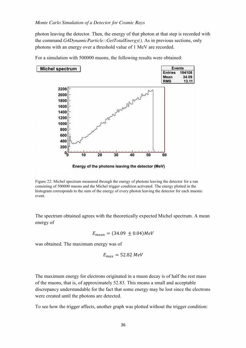
photon leaving the detector. Then, the energy of that photon at that step is recorded with the command G4DynamicParticle::GetTotalEnergy(). As in previous sections, only photons with an energy over a threshold value of 1 MeV are recorded.

For a simulation with 500000 muons, the following results were obtained:

Figure 22: Michel spectrum measured through the energy of photons leaving the detector for a run consisting of 500000 muons and the Michel trigger condition activated. The energy plotted in the histogram corresponds to the sum of the energy of every photon leaving the detector for each muonic event.

The spectrum obtained agrees with the theoretically expected Michel spectrum. A mean energy of

𝐸 = (34.09 ± 0.04)𝑀𝑒𝑉

was obtained. The maximum energy was of

𝐸 = 52.82 𝑀𝑒𝑉

The maximum energy for electrons originated in a muon decay is of half the rest mass of the muons, that is, of approximately 52.83. This means a small and acceptable discrepancy understandable for the fact that some energy may be lost since the electrons were created until the photons are detected.

To see how the trigger affects, another graph was plotted without the trigger condition:


37

Figure 23: Michel spectrum measured through the energy of the photons leaving the detector for a run consisting of 500000 muons without taking into account the Michel trigger condition.

Approximately only 1% of the muons decaying does not fulfill the Michel trigger condition (muon and electron signal within 10 μs). The results for the mean energy and the maximum energy are the same as with the trigger condition enabled.


38

6 Outlook and Summary The subject of this work has been the simulation using Geant4 of a detector for cosmic muons and the comparison of the results obtained with the theoretically expected ones.

All the results obtained agreed with the theoretically expected ones, with the exception of the angular dependence for the intensity of cosmic muons. The reasons for this discrepancy was explained in section 5.2.

Even if some simplifications have been made with respect to the original detector, such as not including all the electronic components, the methods with which measurements are performed in the real detector have been imitated to obtain as realistic as possible results.

Another simplification that has been made is not including photomultipliers in the simulation of the detector. This way photons emitted do not have to enter a certain region to be detected by a photomultiplier and thus registered, but it is enough that they go out of the detector. This was done this way in order to save time, since a simulation where only a small fraction of the photons emitted are considered would have taken too long. A continuation of this work could try to implement this improvements to achieve a higher degree of realism. However, the results obtained should not vary considerably.


39

References [1] C. Grupen. Astroparticle Physics. Springer-Verlag Berlin Heidelberg, 2005.

[2] Burcham and Jobes. Nuclear and Particle Physics. Pearson Education Limited,

1995.

[3] André Röhring. Aufbau und Test eines Detektors für Experimente mit kosmischer

Strahlung. Diplomarbeit, Institut für Kernphysik, University of Münster, Germany,

Münster, 1995.

[4] J. Beringer et al. (Particle Data Group), Phys. Rev. D86, 010001, 2012.

[5] für Praktikumsversuch: Bestimmung der Lebensdauer der Myonen. Institut

für Kernphysik, Technische Universität Darmstadt, Darmstadt, Germany.

[6] C. Berger, Teilchenphysik, eine Einführung. Springer-Verlag Berlin, 1992.

[7] W. R. Leo. Techniques for Nuclear and Particle Physics Experiments. Springer-

Verlag Berlin Heidelberg, 1987.

[8] http://geant4.cern.ch (26/06/2014)

[9] Geant4 User’s Guide for Application Developers. Cern, 2013.

http://geant4.cern.ch/


40

[10] Anleitung für Praktikumsversuch: Ein Detektor für kosmische Strahlung. Institut

für Kernphysik, University of Münster, Germany, Münster.


41


42

I would like to thank Dr. Christian Klein-Bösing for his guidance, as well as Dr. Don Vernekohl and Annika Passfeld for their help.

I would also like to thank my office mates Christian and Katharina for their help with the language and their friendliness.

Vorrei ringraziare i tifosi italiani per essere venuti alla mia presentazione.

También me gustaría agradecer a mi familia su apoyo durante toda mi vida, estos cuatro años de carrera y especialmente este año fuera de casa, especialmente a mis padres, mi hermano Juan y mi hermana Amaia.

Por último me gustaría dar las gracias a todas las personas que me han acompañado durante este año fuera, especialmente a Ángel, Pablo e Isabel en Sevilla, a Giulia en Münster y a Lisa “ovunque”.


43


44

Erklärung des Studierenden

I hereby declare that the script with the title:


has been written by me and no other sources have been used besides the mentioned in the References. Any sections here may be used for other scripts stating that it has been borrowed from this original text.

Hiermit versichere ich, dass die vorliegende Arbeit mit dem Titel:


selbständig verfasst habe, und dass ich keine anderen Quellen und Hilfsmittel als die angegebenen benutzt habe und dass die Stellen der Arbeit, die andere Werken- auch elektronischen Medien- dem Wortlaut oder der Sinn nach entnommen wurden, auf jeden Fall unter Angabe der Quelle als Entlehnung kenntlich gemacht worden sind.

_________________________ _________________________

Ort, Datum Sarazá Canflanca, Pablo

Monte Carlo Simulation of a Detector for Cosmic Rays

Documents

Transcript of Monte Carlo Simulation of a Detector for Cosmic Rays