MCS 1 / 65

Using Monte Carlo Simulation for Project Estimates

Akram Najjar28 July 2016Holiday Inn – DunesBeirut, Lebanon

MCS 2 / 65

First, we state the problem: Why do we need to Simulate?

Second, we discuss the 3 Monte Carlo Simulation Processes:

Process 1: how to prepare a Monte Carlos spreadsheet model

Process 2: how to sample inputs to simulate variety

Process 3: how to analyze the output statistically

10 workouts, will “hopefully” be demonstrated

If time permits: we will demo a Non-PM Monte Carlo Simulations

The Handout and ALL Workouts will be in a Zipped File on www.pmilebanonchapter.org

MCS 4 / 65

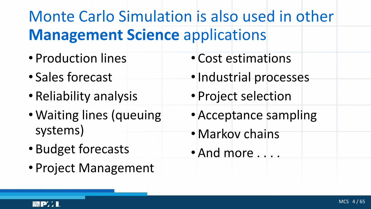
Monte Carlo Simulation is also used in otherManagement Science applications

•Production lines

• Sales forecast

•Reliability analysis

•Waiting lines (queuing systems)

•Budget forecasts

•Project Management

•Cost estimations

• Industrial processes

•Project selection

•Acceptance sampling

•Markov chains

•And more . . . .

MCS 5 / 65

But first . . . . Why use Excel?

• There are 3rd party Monte Carlo Simulation products

• Very few of them deal directly with Project Management

• I only know one that works directly with Microsoft Project (@RISK)

• BUT

• Excel functions are native, out of the box

• Excel is more flexible (much more so if you write VBA code)

• Excel interacts with other environments better

MCS 6 / 65

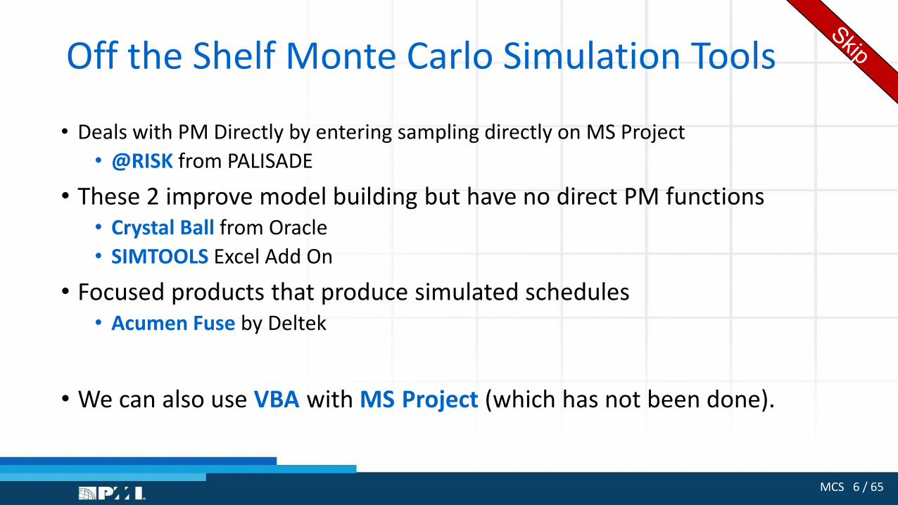
Off the Shelf Monte Carlo Simulation Tools

• Deals with PM Directly by entering sampling directly on MS Project

• @RISK from PALISADE

• These 2 improve model building but have no direct PM functions• Crystal Ball from Oracle

• SIMTOOLS Excel Add On

• Focused products that produce simulated schedules• Acumen Fuse by Deltek

• We can also use VBA with MS Project (which has not been done).

MCS 7 / 65

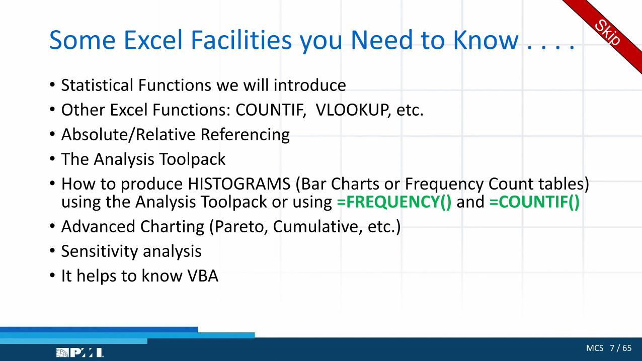
Some Excel Facilities you Need to Know . . . .

• Statistical Functions we will introduce

• Other Excel Functions: COUNTIF, VLOOKUP, etc.

• Absolute/Relative Referencing

• The Analysis Toolpack

• How to produce HISTOGRAMS (Bar Charts or Frequency Count tables) using the Analysis Toolpack or using =FREQUENCY() and =COUNTIF()

• Advanced Charting (Pareto, Cumulative, etc.)

• Sensitivity analysis

• It helps to know VBA

MCS 9 / 65

Why do we Need Monte Carlo Simulation in Project Management?• One of the nightmares of a Project Manager is that he / she needs

Single Values for the following:• Durations

• Resource quantities

• Resource rates

• We call these Single Point Estimates

• The Project Manager has only One Chance to be right . . .

• And he or she will almost never forecast these values correctly . . .

I thought you guys wereWorking on your Project Estimates That’s Exactly what we’re

doing . . . . .

This is what happens when we use the Single Point Estimate Model

A SingleValue forEach InputVariable

One SingleValue for

the OutputVariable

a

b

c

d

IndependentVariables

DependentVariable

Samuel Goldwyn

of MGM

Forecasts are dangerous,

especially those about the future.

The Oracle of Delphi

Greek MythFrom 1600 BC to 300 BC

A Modern JudgmentalForecasting Technique

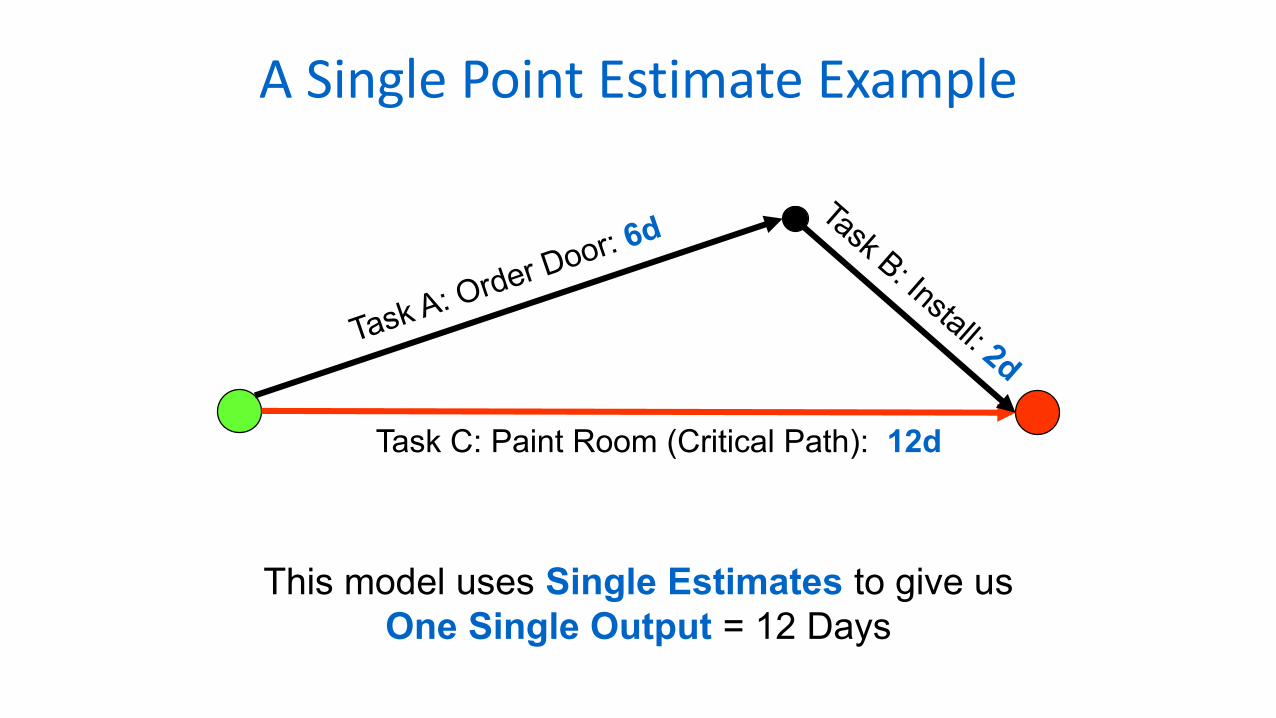
A Single Point Estimate Example

Task C: Paint Room (Critical Path): 12d

This model uses Single Estimates to give us

One Single Output = 12 Days

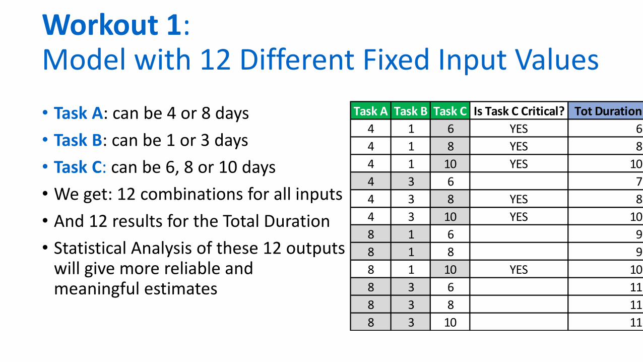
Workout 1: Model with 12 Different Fixed Input Values

• Task A: can be 4 or 8 days

• Task B: can be 1 or 3 days

• Task C: can be 6, 8 or 10 days

• We get: 12 combinations for all inputs

• And 12 results for the Total Duration

• Statistical Analysis of these 12 outputs will give more reliable andmeaningful estimates

Task A Task B Task C Is Task C Critical? Tot Duration

4 1 6 YES 6

4 1 8 YES 8

4 1 10 YES 10

4 3 6 7

4 3 8 YES 8

4 3 10 YES 10

8 1 6 9

8 1 8 9

8 1 10 YES 10

8 3 6 11

8 3 8 11

8 3 10 11

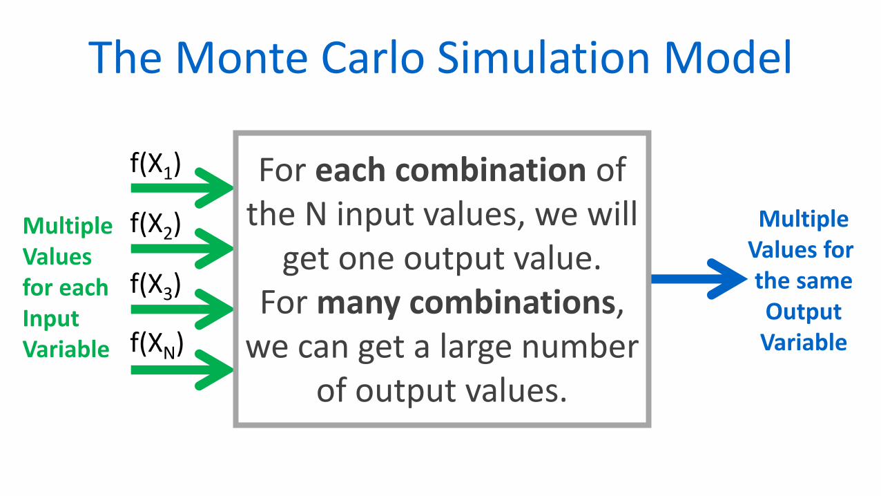
The Monte Carlo Simulation Model

MultipleValues for eachInputVariable

MultipleValues for the sameOutputVariable

For each combination of the N input values, we will

get one output value.For many combinations,

we can get a large number of output values.

f(X1)

f(X2)

f(X3)

f(XN)

MCS 17 / 65

By using different combinations of values for the input variables, we will get a large number of values for the output variable. (The Delphi Oracle?)

We can then analyze the output values statistically.

Our forecast will be “educated” and not a “shot in the dark”.

MCS 18 / 65

Process 1:How to Setup a Monte Carlo Spreadsheet to allow the Model to calculate a large number of Global Outputs using the large number of combined Inputs

MCS 19 / 65

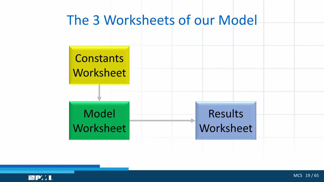
The 3 Worksheets of our Model

ModelWorksheet

ConstantsWorksheet

ResultsWorksheet

MCS 20 / 65

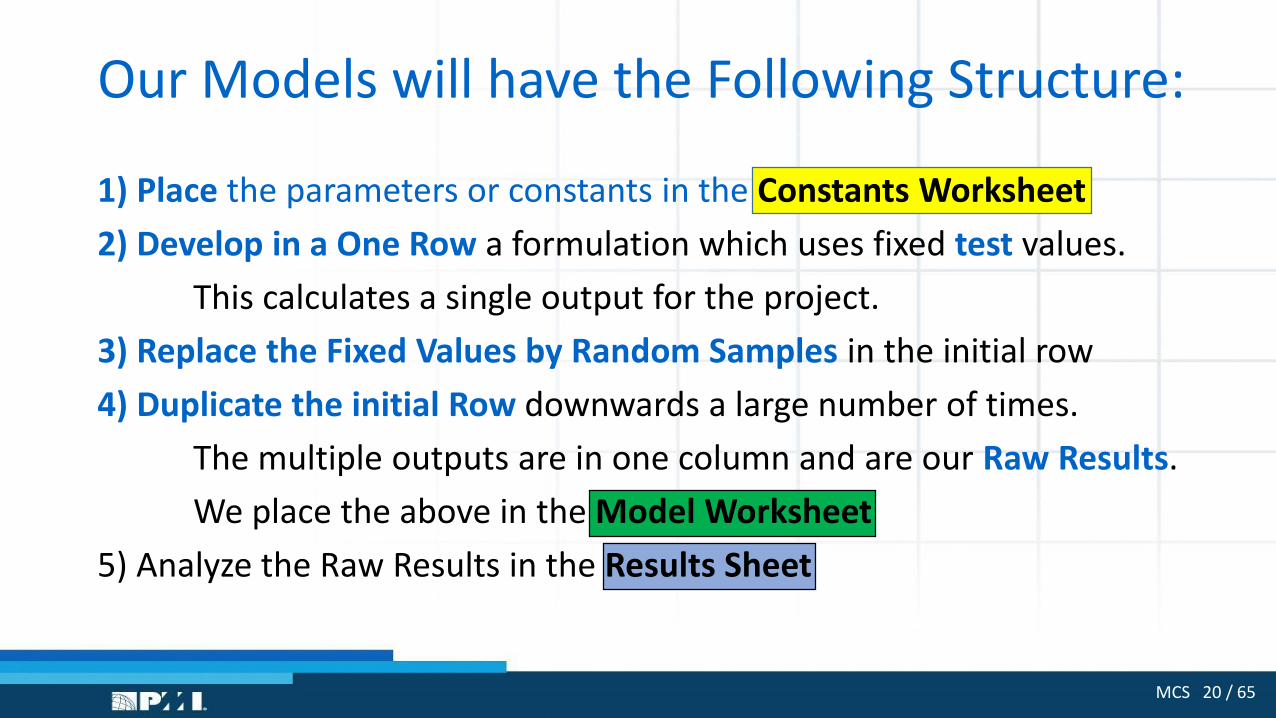
Our Models will have the Following Structure:

1) Place the parameters or constants in the Constants Worksheet

2) Develop in a One Row a formulation which uses fixed test values.

This calculates a single output for the project.

3) Replace the Fixed Values by Random Samples in the initial row

4) Duplicate the initial Row downwards a large number of times.

The multiple outputs are in one column and are our Raw Results.

We place the above in the Model Worksheet

5) Analyze the Raw Results in the Results Sheet

MCS 21 / 65

Workout 2: An Equipment Costing Modelto Demonstrate our Global Procedure

• Row 2 shows the calculation of the total cost using the Random Samples from a BetaPERT distribution

• The Total Cost = • Equipment Cost +

• Spares for 3 years +

• Yearly Maintenance = a % of the Cost of the Equipment

• Rows 3 to 1002 duplicate Row 2 to generate 1000 outputs

• Col G is the total cost and has our 1000 Raw Results

MCS 22 / 65

Process 2:

How to Use Excel’s Functions to generate multiple samples that comply with the behavior of a specific input f(X1)

MCS 23 / 65

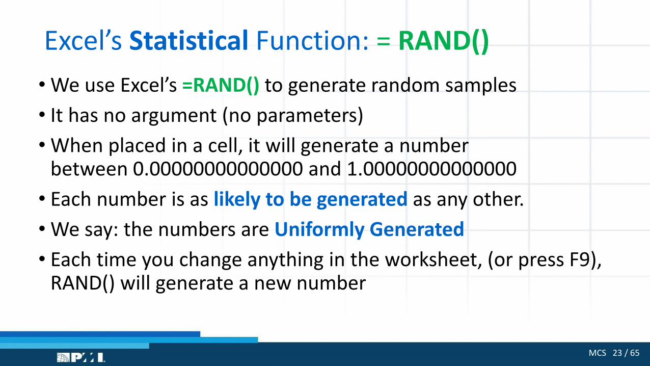
Excel’s Statistical Function: = RAND()

• We use Excel’s =RAND() to generate random samples

• It has no argument (no parameters)

• When placed in a cell, it will generate a number between 0.00000000000000 and 1.00000000000000

• Each number is as likely to be generated as any other.

• We say: the numbers are Uniformly Generated

• Each time you change anything in the worksheet, (or press F9), RAND() will generate a new number

MCS 24 / 65

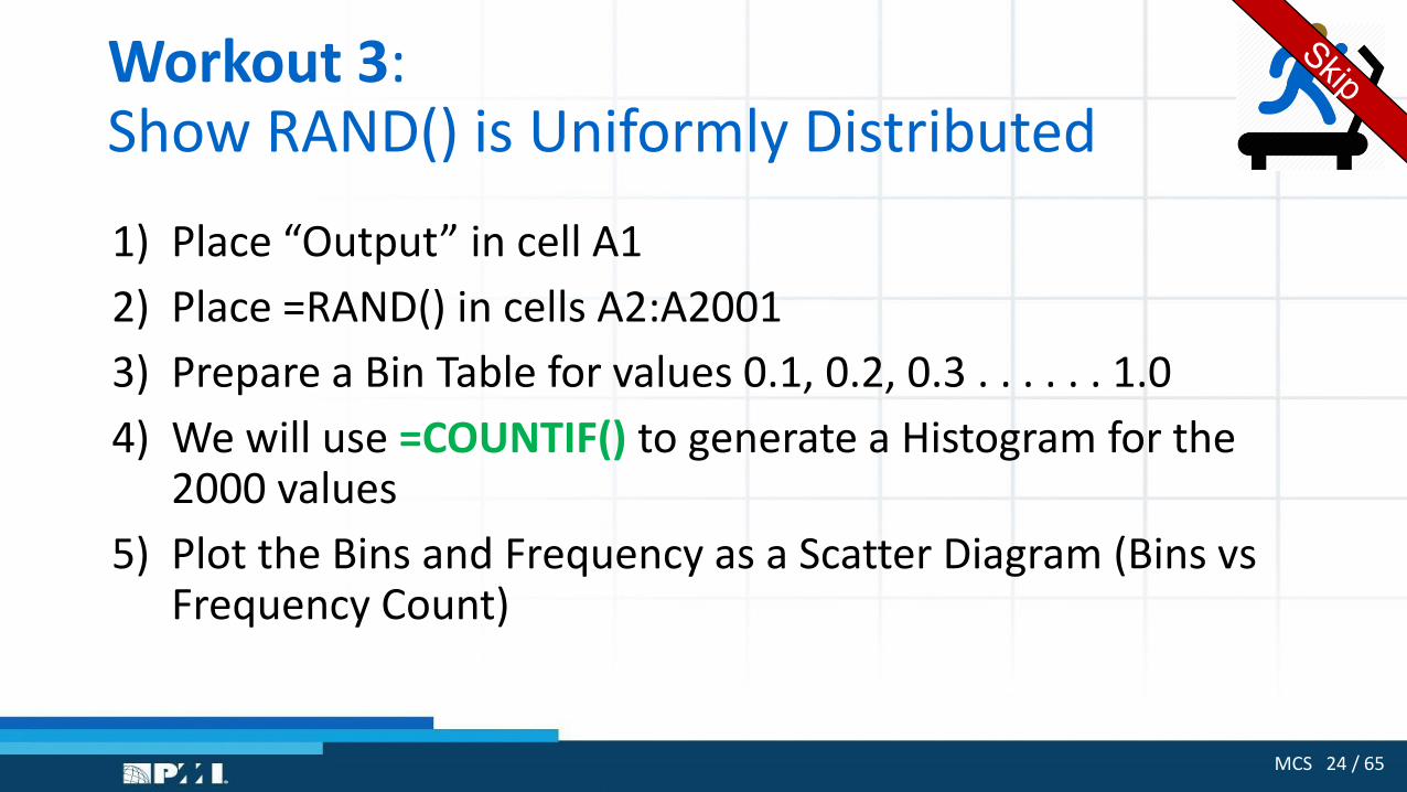
Workout 3: Show RAND() is Uniformly Distributed

1) Place “Output” in cell A1

2) Place =RAND() in cells A2:A2001

3) Prepare a Bin Table for values 0.1, 0.2, 0.3 . . . . . . 1.0

4) We will use =COUNTIF() to generate a Histogram for the 2000 values

5) Plot the Bins and Frequency as a Scatter Diagram (Bins vs Frequency Count)

MCS 25 / 65

How to Use RAND()

to Generate Samples

that are Uniformly Distributed

over other ranges than 0 and 1?

MCS 26 / 65

What is a Uniform Distribution?

• Many project parameters follow a uniform distribution

• A given input variable would vary from A (lower) to B (upper)

• Each value between A and B is equally likely to arise

• Example: • A price can range from $10.00 to $14.00 : UNIFORMLY

• The duration of a task can vary from 5.00 to 7.00 days : UNIFORMLY

MCS 27 / 65

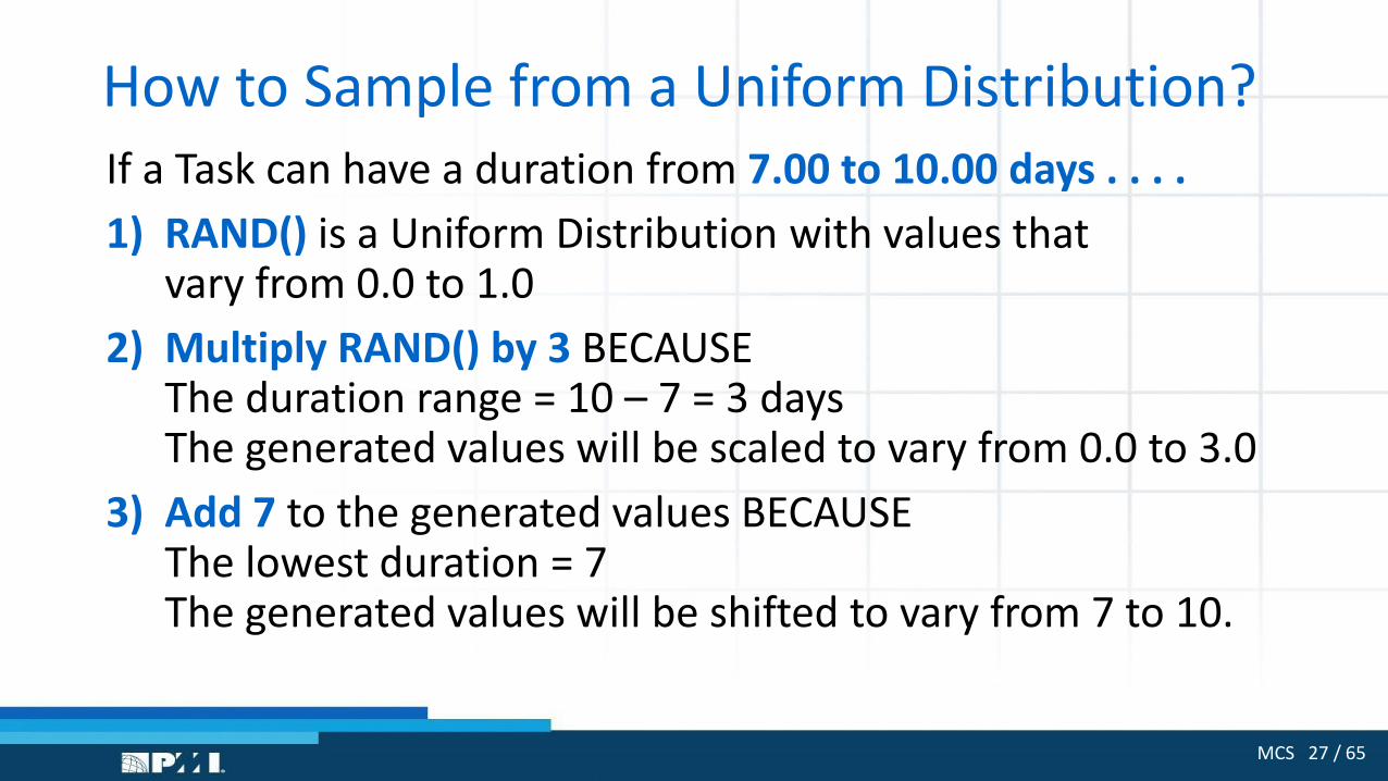
How to Sample from a Uniform Distribution?If a Task can have a duration from 7.00 to 10.00 days . . . .

1) RAND() is a Uniform Distribution with values that vary from 0.0 to 1.0

2) Multiply RAND() by 3 BECAUSEThe duration range = 10 – 7 = 3 days The generated values will be scaled to vary from 0.0 to 3.0

3) Add 7 to the generated values BECAUSE The lowest duration = 7The generated values will be shifted to vary from 7 to 10.

Generating Uniformly Distributed Numbers from 7 to 10

Using RAND() from 0 to 10

3

0

1

= RAND() x 3

= RAND() x 3 + 7

7

10

=RAND()

MCS 29 / 65

Our Formula for Generating Uniformly Distributed Values between A (Lower) and B (Higher):

Generated Value = RAND() * (B – A) + A= RAND() * Range + A

In Excel, it is best to place A and B in a Constants Sheet

And to calculate the Range = (B – A) to simplify formulas.

The next Workout will demonstrate the use of this formula

MCS 30 / 65

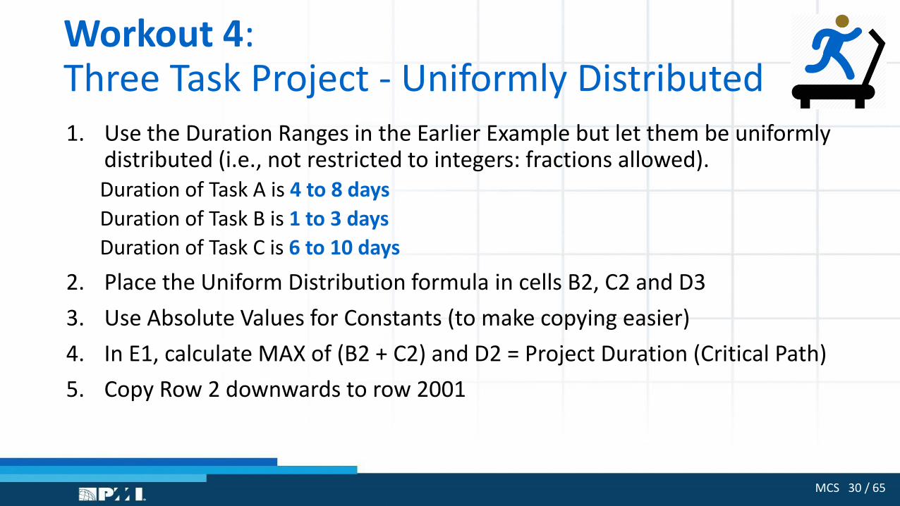
Workout 4:Three Task Project - Uniformly Distributed1. Use the Duration Ranges in the Earlier Example but let them be uniformly

distributed (i.e., not restricted to integers: fractions allowed).Duration of Task A is 4 to 8 days

Duration of Task B is 1 to 3 days

Duration of Task C is 6 to 10 days

2. Place the Uniform Distribution formula in cells B2, C2 and D3

3. Use Absolute Values for Constants (to make copying easier)

4. In E1, calculate MAX of (B2 + C2) and D2 = Project Duration (Critical Path)

5. Copy Row 2 downwards to row 2001

MCS 31 / 65

Bar Charts, Frequency Tables and HistogramsAre the Same Thing . . . . Step 1: collect the raw data or results in Col A (Results sheet)

Step 2: specify categories in which we group similar raw data.These categories are also called: Bins

These can be durations, resource rates or resource quantities

Step 3: use =COUNTIF() to classify our Raw Results into the Bins

Step 4: next to the frequencies of the Bins, find the % Frequency

Step 5: next to the % Frequency, find the Cumulative Frequency %

Workout 4a:The Basis of our Analysis is the Frequency Table

Part of a Table of Observations(Raw Data)

Heights

170

145

174

144

140

182

188

157

188

187

. . . .

. . . .

Height

Categories

Frequency

Count

120 0

130 0

140 2

150 3

160 21

170 35

180 22

190 14

200 3

210 0

220 0

MCS 33 / 65

The Next “Basis” is the Cumulative Chart

Height

Categories

Frequency

Count

Frequeny

%

Cum %

120 0 0% 0%

130 0 0% 0%

140 2 2% 2%

150 3 3% 5%

160 21 21% 26%

170 35 35% 61%

180 22 22% 83%

190 14 14% 97%

200 3 3% 100%

210 0 0% 100%

220 0 0% 100%

MCS 34 / 65

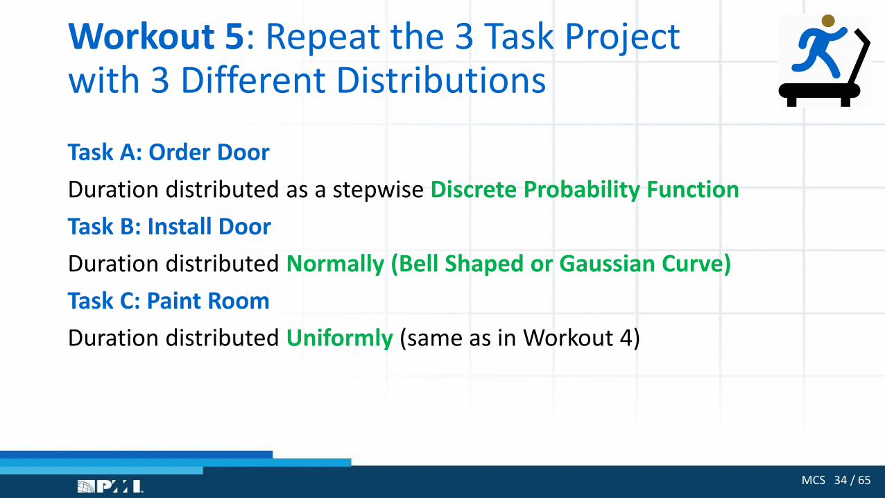
Workout 5: Repeat the 3 Task Project with 3 Different Distributions

Task A: Order Door

Duration distributed as a stepwise Discrete Probability Function

Task B: Install Door

Duration distributed Normally (Bell Shaped or Gaussian Curve)

Task C: Paint Room

Duration distributed Uniformly (same as in Workout 4)

An Example of the 3 Tasks with 3 Different Distributions for the 3 Durations

30 %

50 %

20 %

NormalDistribution

Discreet ProbabilityDistribution

Uniform Distribution

A: Order Door B: Install Door

C: Paint Room

6 10

MCS 36 / 65

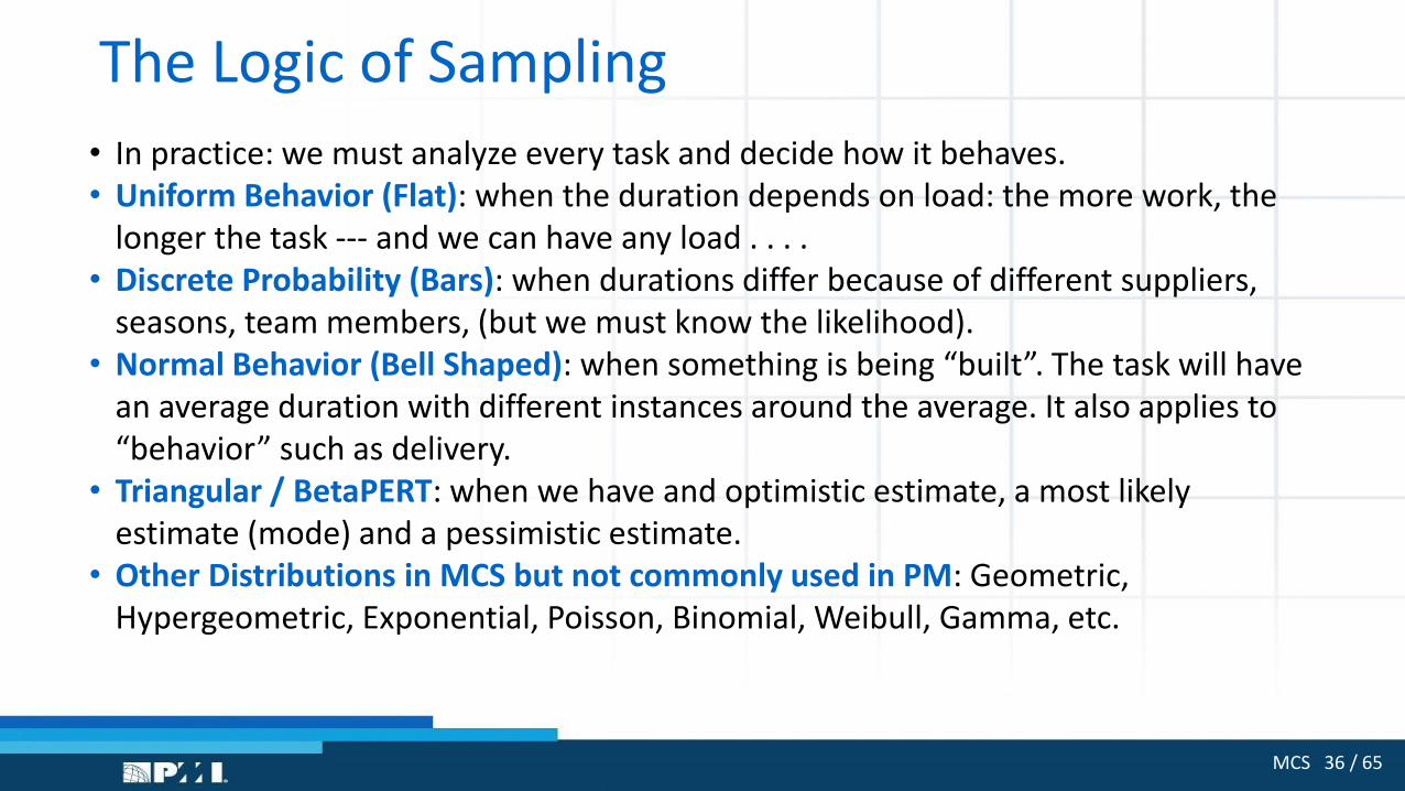
The Logic of Sampling

• In practice: we must analyze every task and decide how it behaves.• Uniform Behavior (Flat): when the duration depends on load: the more work, the

longer the task --- and we can have any load . . . .• Discrete Probability (Bars): when durations differ because of different suppliers,

seasons, team members, (but we must know the likelihood).• Normal Behavior (Bell Shaped): when something is being “built”. The task will have

an average duration with different instances around the average. It also applies to “behavior” such as delivery.

• Triangular / BetaPERT: when we have and optimistic estimate, a most likely estimate (mode) and a pessimistic estimate.

• Other Distributions in MCS but not commonly used in PM: Geometric, Hypergeometric, Exponential, Poisson, Binomial, Weibull, Gamma, etc.

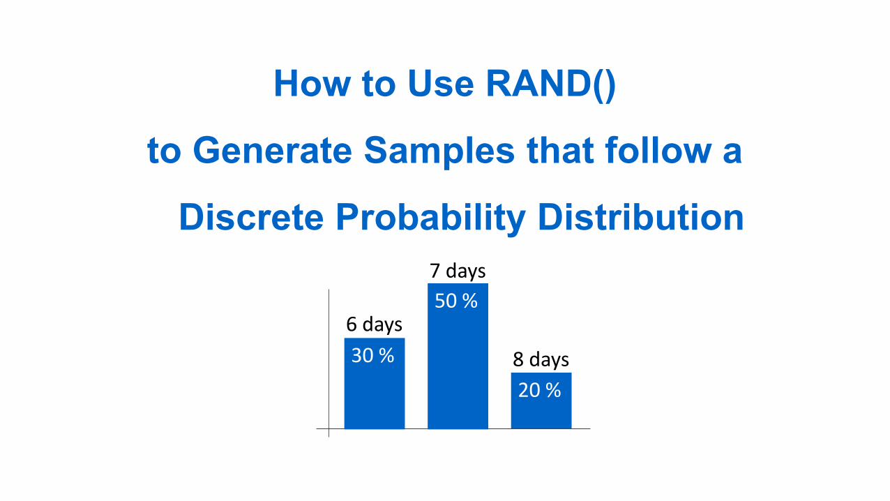
How to Use RAND()

to Generate Samples that follow a

Discrete Probability Distribution

30 %

6 days50 %

7 days

20 %

8 days

MCS 38 / 65

What is a Discrete Probability Distribution?

• Inputs may have different values: prices, durations, rates, quantities

• There is a an associated probability for the occurrence of each input

• Example 1 – The Cost Price: 10% of the time, it will be $12.5 while for 40% it will be $13 and for 50% it will be $13.5

• Example 2 – The Duration: sometimes 4 days (35% of the time), sometimes 6 days (40% of the time) and sometimes 8 days (25%).

• If categories > 4 we have to use =VLOOKUP() else use Nested IF()

• Why? because Nest IF’s gets complicated with more than 4 nests

• Also, you are limited to nest 7 times in an IF() expression

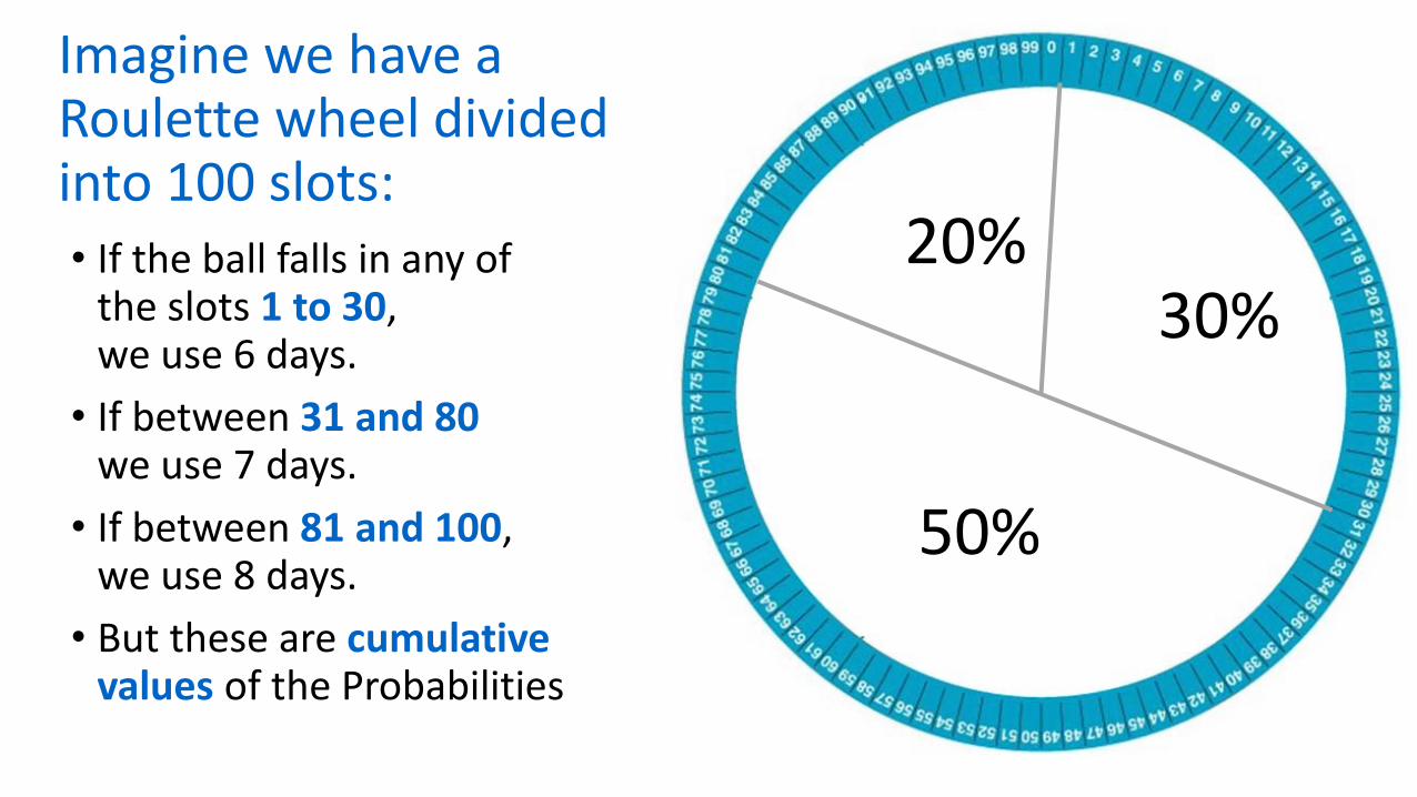
Discrete Probabilities for the Duration of Task A - Order Door:

30% of the time, the Duration will be = 6 days50% of the time, the Duration will be = 7 days20% of the time, the Duration will be = 8 days

50%

20%30%

Imagine we have a Roulette wheel divided into 100 slots:• If the ball falls in any of

the slots 1 to 30, we use 6 days.

• If between 31 and 80 we use 7 days.

• If between 81 and 100, we use 8 days.

• But these are cumulative values of the Probabilities

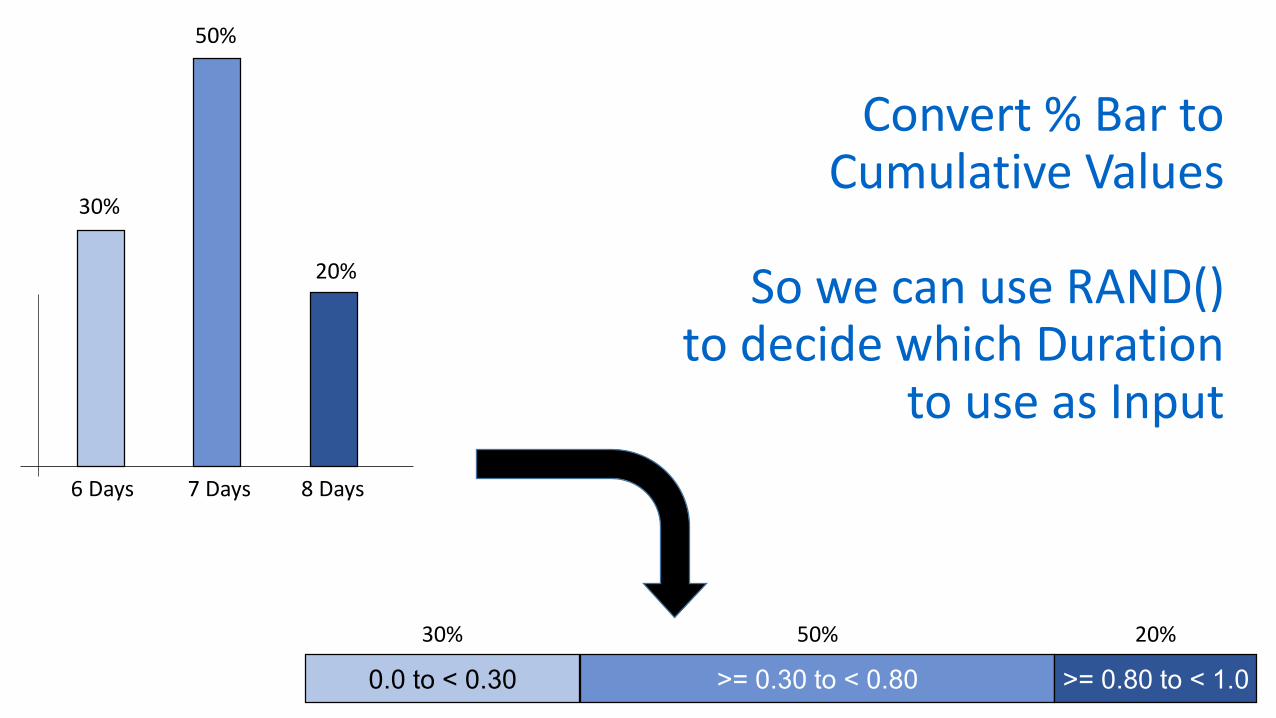
Convert % Bar to Cumulative Values

So we can use RAND() to decide which Duration

to use as Input

0.0 to < 0.30 >= 0.30 to < 0.80 >= 0.80 to < 1.0

6 Days 7 Days 8 Days

30%

50%

20%

30% 50% 20%

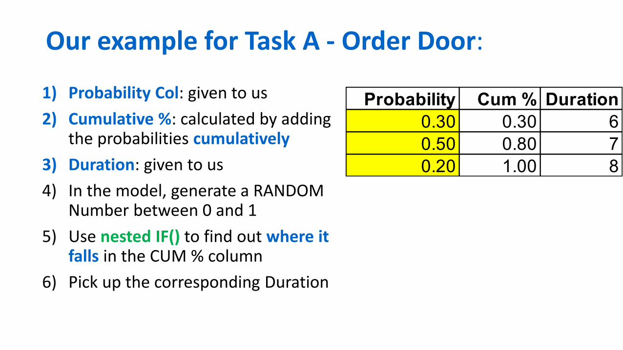
Our example for Task A - Order Door:

1) Probability Col: given to us

2) Cumulative %: calculated by adding the probabilities cumulatively

3) Duration: given to us

4) In the model, generate a RANDOM Number between 0 and 1

5) Use nested IF() to find out where it falls in the CUM % column

6) Pick up the corresponding Duration

Probability Cum % Duration

0.30 0.30 6

0.50 0.80 7

0.20 1.00 8

MCS 43 / 65

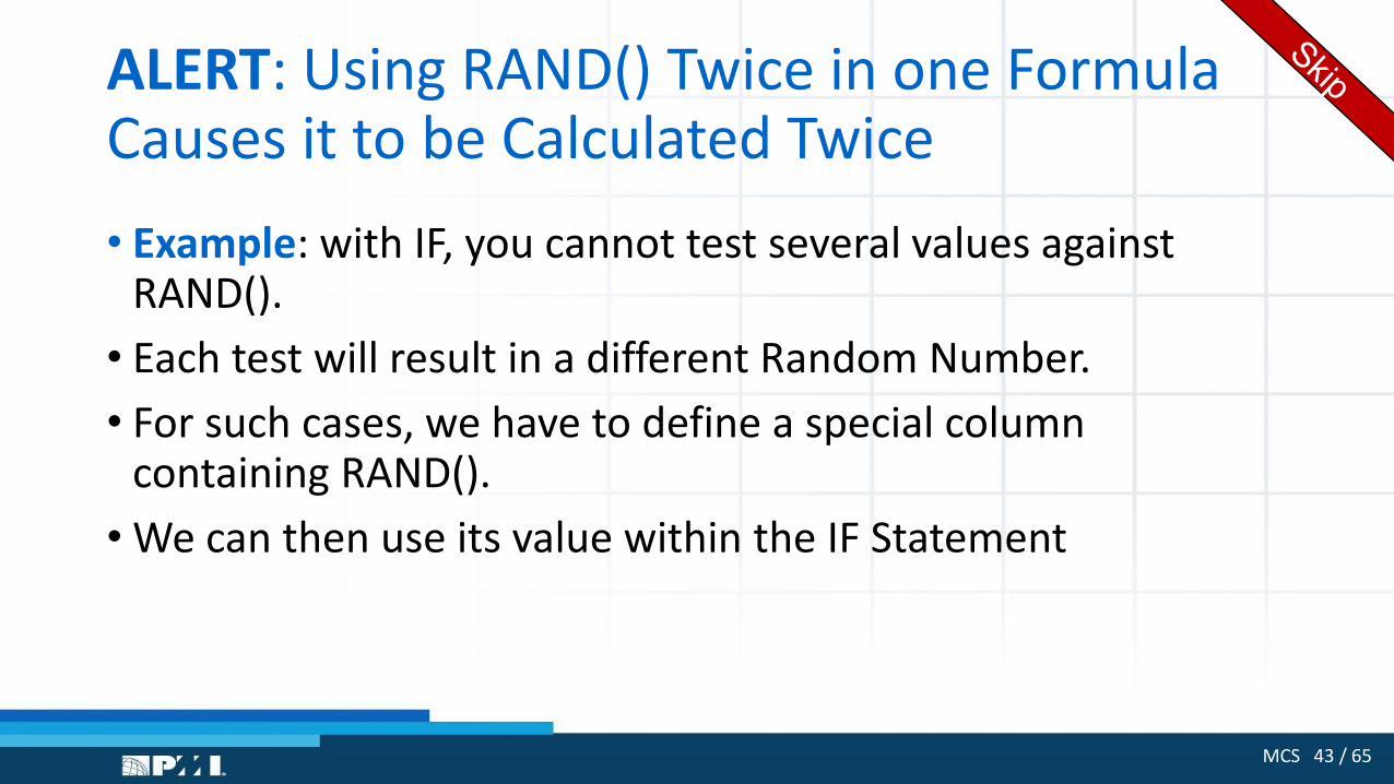
ALERT: Using RAND() Twice in one Formula Causes it to be Calculated Twice

• Example: with IF, you cannot test several values against RAND().

• Each test will result in a different Random Number.

• For such cases, we have to define a special column containing RAND().

• We can then use its value within the IF Statement

MCS 44 / 65

Using NESTED IF() To Generate Discrete Probability Values

=IF(A2<F2, G2, IF(A2<F3, G3, G4) )

MCS 45 / 65

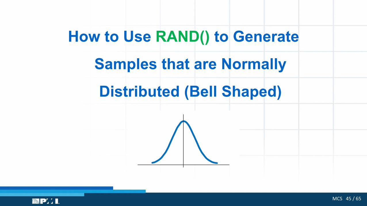
How to Use RAND() to Generate

Samples that are Normally

Distributed (Bell Shaped)

MCS 46 / 65

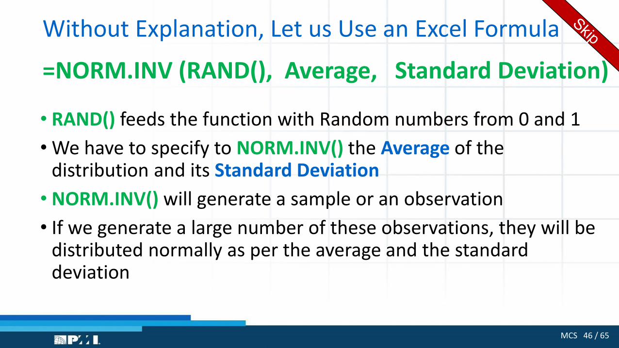
Without Explanation, Let us Use an Excel Formula

=NORM.INV (RAND(), Average, Standard Deviation)

• RAND() feeds the function with Random numbers from 0 and 1

• We have to specify to NORM.INV() the Average of the distribution and its Standard Deviation

• NORM.INV() will generate a sample or an observation

• If we generate a large number of these observations, they will be distributed normally as per the average and the standard deviation

MCS 47 / 65

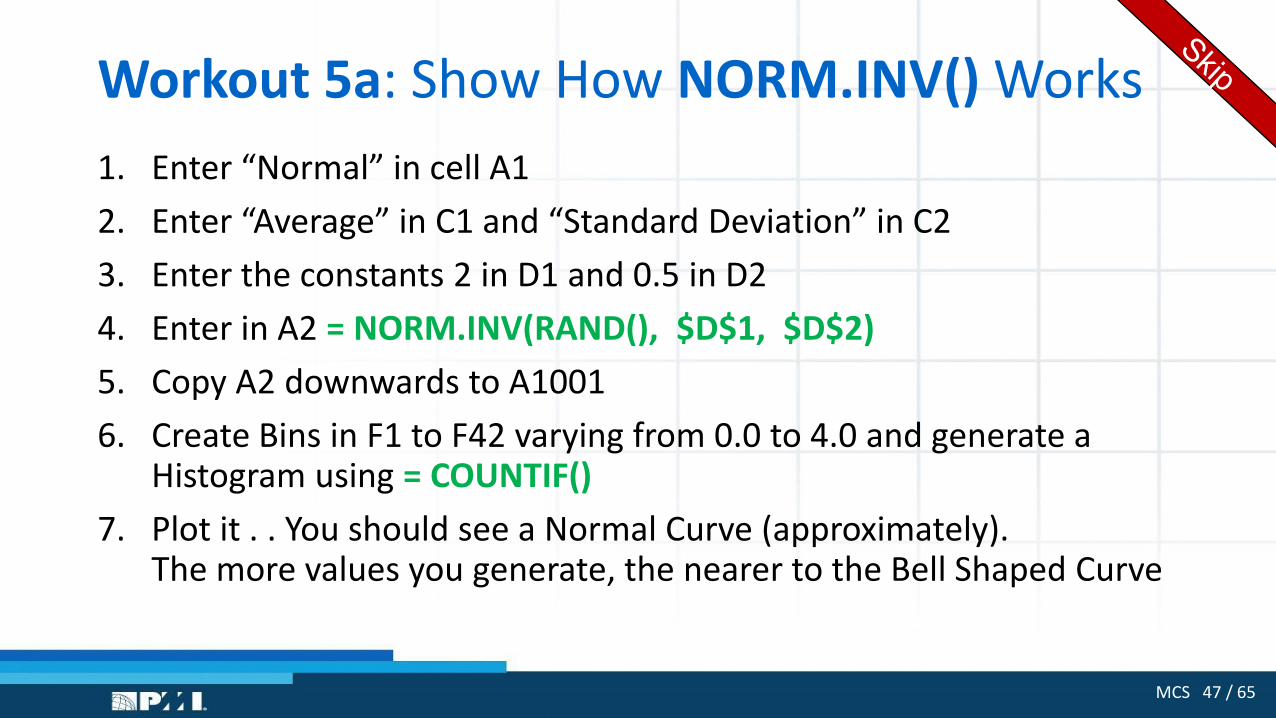
Workout 5a: Show How NORM.INV() Works

1. Enter “Normal” in cell A1

2. Enter “Average” in C1 and “Standard Deviation” in C2

3. Enter the constants 2 in D1 and 0.5 in D2

4. Enter in A2 = NORM.INV(RAND(), $D$1, $D$2)

5. Copy A2 downwards to A1001

6. Create Bins in F1 to F42 varying from 0.0 to 4.0 and generate a Histogram using = COUNTIF()

7. Plot it . . You should see a Normal Curve (approximately). The more values you generate, the nearer to the Bell Shaped Curve

MCS 48 / 65

Workout 6: Monte Carlo Simulation

for a Project with 14 Tasks

(And 4 Nodes in the Network)

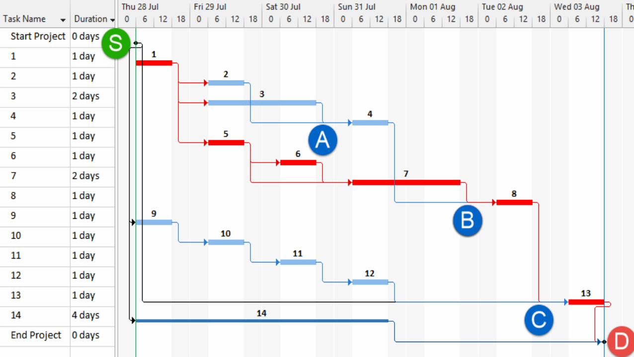
The MicrosoftProject Plan

MCS 50 / 65

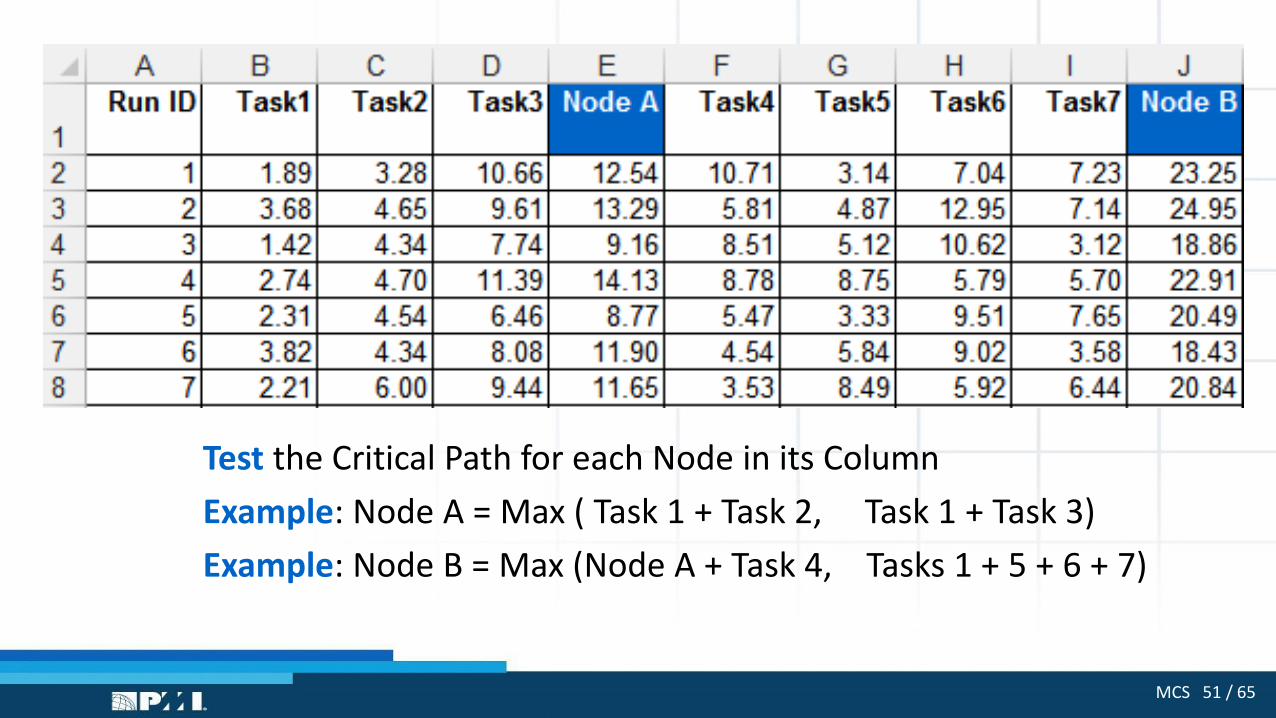
Mathematically, we Can Define a Project as Columns in Excel1. Identify Each Node where parallel paths meet

We have 1 Start Node and 4 other Nodes (and the End Project = D).

2. Create a Column for each Task

3. Create a Column for each Node to be placed after the Tasks that meet at it.

4. Place the Duration sampling function of each Task in its Column

5. In each Node cell, enter the =MAX() function to find the Critical Path of the Tasks before it (see next slide for Nodes A and B)

MCS 51 / 65

Test the Critical Path for each Node in its Column

Example: Node A = Max ( Task 1 + Task 2, Task 1 + Task 3)

Example: Node B = Max (Node A + Task 4, Tasks 1 + 5 + 6 + 7)

MCS 52 / 65

The Logic of the Model

• In Each Model we have to analyze the behavior of EACH Task

• We then decide which Statistical Distribution best describes the Duration

• For simplicity: we will start with the Uniform Distribution for ALL tasks - but with different parameters

• We then use the Normal and BetaPERT distributions

• And another model with a Mixture of distributions

• Let us review the Triangular and the BetaPERT Distributions

MCS 53 / 65

Workout 6a: The Triangular and BetaPERT Distributions• We favor optimistic estimates because of fear, psychology and

managerial pressure

• We might guess the cost of a cubic meter of concrete = $130

• Under fear, psychology and pressure, we will favor a cost = $110

• But we will strongly resist an estimate = $160

• Most LATE projects are really projects which are UNDERESTIMATED

• Most OVER-BUDGET projects are really UNDERESTIMATED

MCS 54 / 65

What do we Need for the PERT Estimate, the Triangular and BetaPERT Distributions?

• We need • An optimistic estimate

• A most likely estimate

• A pessimistic estimate

• A distribution is positively skewed if more of its observations are low

• A distribution is negatively skewed if more of its observations are high

MCS 55 / 65

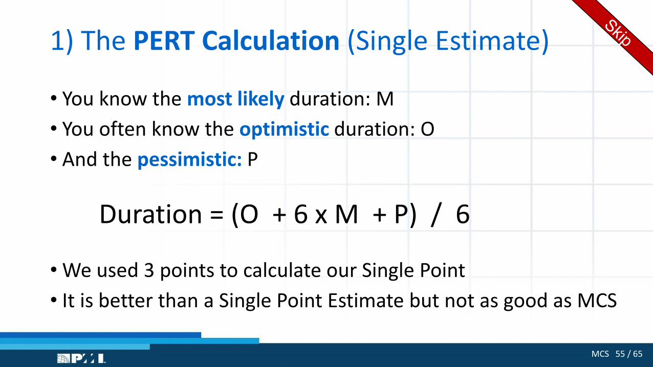
1) The PERT Calculation (Single Estimate)

• You know the most likely duration: M

• You often know the optimistic duration: O

• And the pessimistic: P

Duration = (O + 6 x M + P) / 6

• We used 3 points to calculate our Single Point

• It is better than a Single Point Estimate but not as good as MCS

MCS 56 / 65

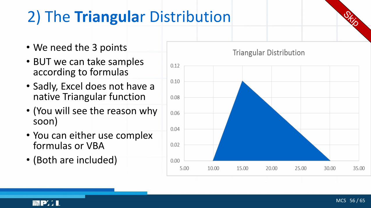
2) The Triangular Distribution

• We need the 3 points

• BUT we can take samples according to formulas

• Sadly, Excel does not have a native Triangular function

• (You will see the reason why soon)

• You can either use complex formulas or VBA

• (Both are included)

MCS 57 / 65

3) The BetaPERT Function

• Mathematically, this is quite complex but is available in Excel

• Advantage: it does not have a sharp peak

• Advantage: it slopes down smoothly (to the right and to the left)

• We now see why Microsoft did not include the Triangular function

• The 3 parameters have different names in the industry• The optimistic = minimum

• The most likely = mode

• The pessimistic = maximum

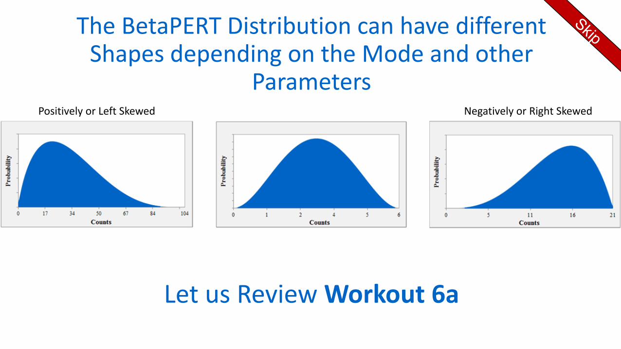
The BetaPERT Distribution can have different Shapes depending on the Mode and other

Parameters

Let us Review Workout 6a

Positively or Left Skewed Negatively or Right Skewed

MCS 59 / 65

Workout 7: (if time permits)Budget Forecasting• The budget forecast is complex

• It is formulated in the Model worksheet

• Our Input Variables are 8 growth rates varied using different distributions (found in the Constants worksheet)

• The outputs to be analyzed are then duplicated in the Runs worksheet

MCS 60 / 65

Process 3: How to Use Excel’s Functions and Charts to Statistically Analyze the large number of Outputs generated by the MCS Model

MCS 61 / 65

The Analysis: 1) Convert and Move Dynamic to Static Results• The Input Data in the Model Sheet is Dynamic

• Because RAND() is found in the formulas, the raw data keeps changing

• When something happens in the Workbook or when we press F9

• The Results in the Model will also be Dynamic

• We cannot analyze Dynamic Results!

• Solution: copy the Results column from the Model to the Result worksheet• BUT, Paste as Values, i.e., without formulas

• This freezes the data in the Results worksheet

MCS 62 / 65

The Analysis: 2) Prepare a Histogram for the Results1) Decide on the number of Bins (grouping of results

• Usually from 10 to 30

2) Generate a Frequency Table (Histogram) from the Raw Data using:• The =FREQUENCY() function OR

• The =COUNTIF() function (only if results are integers) OR

• The Analysis Toolpack (if you are a masochist)

3) Generate the Cumulative % of the Frequency Count

4) Generate the Bar Chart + Cumulative % (Pareto)• Show a Bar Chart for the Frequency Count (Histogram)

• On the same chart, show the cumulative % of the counts (Pareto)

MCS 63 / 65

The Analysis: 3) Show the Descriptive Statistics

• Use the Analysis Toolpack

• Generate the Descriptive Statistics

• These give a variety of analyses about the Raw Data

MCS 64 / 65

The Analysis: 4) Manipulate The Model

• Change the constants

• Change the distributions

• Elaborate the calculations

• Why play with the model?• To verify the results

• To ensure they are close to reality

• To vary the reality model so we can get “What If” sensitivity

Thank You!