Monte Carlo Techniques in Radiation Detection and Measurement.

Prooress in Nuclear Energy. Vol. 14, No. 3, pp. 26%299, 1984. 0149 1970"84 $0.00+ .50 Printed in Great Britain. All rights reserved. Copyrighl ~ 1984 Pergamon Press Ltd.
MONTE CARLO METHODS FOR RADIATION TRANSPORT ANALYSIS ON VECTOR COMPUTERS
FORREST B. BROWN* and WILLIAM R. MARTIN
Department of Nuclear Engineering, University of Michigan, Ann Arbor, Michigan, U.S.A.
(Received 17 July 1984)
Abstract The development of advanced computers with special capabilities for vectorized or parallel calculations demands the development of new calculational methods. The very nature of the Monte Carlo process precludes direct conversion of old (scalar) codes to the new machines. Instead, major changes in global algorithms and careful selection of compatible physics treatments are required. Recent results for Monte Carlo in multigroup shielding applications and in continuous-energy reactor lattice analysis have demonstrated that Monte Carlo methods can be successfully vectorized. The significant effort required for stylized coding and major algorithmic changes is worthwhile, and significant gains in computational efficiency are realized. Speedups of at least twenty to forty times faster than CDC-7600 scalar calculations have been achieved on the CYBER-205 without sacrificing the accuracy of standard Monte Carlo methods. Speedups of this magnitude provide reductions in statistical uncertainties for a given amount of computing time, permit more detailed and realistic problems to be analyzed, and make the Monte Carlo method more accessible to nuclear analysts. Following overviews of the Monte Carlo method for particle transport analysis and of vector computer hardware and software characteristics, both general and specific aspects of the vectorization of Monte Carlo are discussed. Finally, numerical results obtained from vectorized Monte Carlo codes run on the CYBER-205 are presented.
I. INTRODUCTION
Random walk Monte Carlo calculations are a mainstay of radiation transport analysis in nuclear engineering. Although Monte Carlo calculations of neutron and/or gamma-ray transport are time- consuming and expensive, they constitute the only feasible means of solving many problems with compli- cated geometry and/or interaction probabilities, and are valuable in providing calculational standards for validating approximate calculational methods. For both fission and fusion reactor shielding analyses, Monte Carlo methods can readily accommodate complex 3-dimensional configurations including cones, tori and internal voids. In reactor physics analysis Monte Carlo calculations represent ' t ruth ' against which approximate calculational methods may be calibrated. The Monte Carlo method permits the exact modelling of problem geometry, a highly accurate mathematical model for particle interactions with matter, and a cross-section representation that is as accurate as theory and measurement permit.
Conventional (scalar) Monte Carlo codes simulate the complete history of a single particle by repeated
* Current address: Knolls Atomic Power Laboratory, Schenectady, New York, N.Y. 12301, U.S.A.
269
tracking through the problem geometry and by random sampling from probability distributions that represent the collision physics. The precision of Monte Carlo results is primarily limited by the computing time required to obtain acceptable statistical uncer- tainties. The accumulation of data from particle histories in the Monte Carlo analysis of a typical problem may sometimes require several hours (or possibly days) of CDC-7600 C P U time to achieve acceptable small statistical uncertainties. A straight- forward conversion of scalar Monte Carlo codes to advanced computers such as the CYBER-205 and CRAY-1 may typically result in codes which run between one and two times faster than on a CDC-7600 (with some tailoring of the coding). This speedup is due primarily to the reduced cycle time and improved architecture of the scalar processors.
With computer execution time as the only signifi- cant drawback to Monte Carlo calculations, it is natural to consider using the vector processing capa- bilities of current supercomputers such as the CRAY-1 or CYBER-205 to speed up Monte Carlo calculations. There is an important difference, however, between the new supercomputers and previous machines: al though the vector computers are much faster, their full potential speed is attainable only in 'vectorized'
270 F.B. BROWY and W. R. MARTIN
calculations (i.e. non-recursive operations on ordered data arrays). Monte-Carlo codes, however, are ill- suited for direct vectorization. The random nature of the Monte Carlo method seems to be at odds with the demands of vector processing, where identical opera- tions must be performed on streams of contiguous data (vectors). The probabilistic nature of the calculation results in coding with few loops and very many conditional statements, which inhibit vector process- ing. This is illustrated by examining a flowchart for a typical Monte Carlo code, which shows little structure to be exploited through vector operations. To a large degree, this state of affairs is due to the capabilities of previous computers used for Monte Carlo: it is natural to follow the history of one particle at a time on a machine which can only perform one calculation at a time. The development of advanced computers with special capabilities for vectorized calculations de- mands the development of new calculational methods. The very nature of Monte Carlo calculations precludes direct conversion to the new machines through the use of automatic vectorization software or simple re- coding by programmers. Indeed, the effective vectoriz- ation of Monte Carlo can be achieved only through major changes in global algorithms and careful selection of compatible physics treatments.
Early known efforts to vectorize Monte Carlo calculations for vector computers were either unsuc- cessful or, at best, achieved speedups on the order of seven to ten for highly simplified problems (see Brown, 1981a). Recent results for Monte Carlo in multigroup shielding applications (Brown, 1981a; Brown et al., 198 lb) and in continuous-energy reactor lattice analy- sis (Brown, 1982, 1983; Brown and Mendelson, 1984) have demonstrated that Monte Carlo can be success- fully vectorized for the CYBER-205 computer. Speedups in the range of 20 to 40 times faster than CDC-7600 scalar calculations have been achieved on the CYBER-205 with no degradation in the accuracy of the standard Monte Carlo methods. Speedups of this magnitude provide reductions in statistical uncer- tainties for a given amount of computing time, permit more detailed and realistic problems to be analyzed, and make the Monte Carlo method more accessible to nuclear analysts. Moreover, the impact of a 'turn- around time' measured in hours versus days (or even weeks) for a scientist/engineer cannot be minimized.
Following overviews of the Monte Carlo method for particle transport analysis and of vector computer hardware and soflware characteristics, both general and specific aspects of the vectorization of Monte Carlo will be discussed. The primary basis for the methods and results discussed throughout is the authors' experience in developing several vectorized
Monte Carlo codes. Seminal investigations of funda- mental techniques were performed at the University of Michigan and led to the development of MCVMG, a vectorized multigroup Monte Carlo code for reactor shielding applications intended to demonstrate the potential of the new methods. Later work at Knolls Atomic Power Laboratory (KAPL) led to the develop- ment of MCV, a vectorized continuous-energy Monte Carlo code which is used for the analysis of neutron transport in nuclear reactors.
1.1. The Monte Carlo method for radiation transport analysis
The Monte Carlo method is the most general and powerful numerical method available for solving neutron and gamma-ray transport problems. In sharp contrast to other methods such as discrete ordinates, integral transport, finite difference and finite element methods, the Monte Carlo method imposes no a priori restrictions on problem geometry nor on the detail which may be used to describe physical events. Indeed, the Monte Carlo method is frequently formulated as a stochastic numerical model of physical phenomena, without attempting rigorous derivation of an appro- priate 'transport equation' (Cashwell and Everett, 1957). There is, however, an extensive literature devoted to Monte Carlo which provides a sound theoretical basis (Carter and Cashwell, 1975; Hammersley and Handscomb, 1967; Kahn, 1956a; McGrath et al., 1975; Schreider, 1966; Spanier and Gelbard, 1969). Considering the complexity of current designs for fission reactors, fusion devices, and radi- ation shielding, a growing percentage of particle transport calculations requires detailed 3-dimensional analyses. Monte Carlo is especially suited to these needs and is presently the only method capable of treating complicated 3-dimensional geometry in a reasonable amount of computing time. Since there are many references on both the physical and mathemat- ical bases for the Monte Carlo method, this overview will concentrate on summarizing the major features relevant to vectorizing the Monte Carlo calculations.
A convenient starting point for discussing Monte Carlo is the integral form of the linear time- independent Boltzman transport equation, written here in terms of the collision density, ~,
ip(r,v) =
I[S ~9 (r',v')C (v '~ v ;r')dv' + Q(r',v)] T ( r ' ~ r ;v) dr',
where r is position, v is particle velocity, qJ is the density of collisions, and Q is a source term. Two kernels arise

Monte Carlo methods on vector computers 271
in the above integral equation, a collision kernel, C, and a transport kernel, T. The collision kernel includes processes which may either alter particle energy and direction or lead to particle absorption and possible secondary particle emission. The transport kernel includes processes which affect particle position, i.e. streaming until a collision occurs or a boundary is crossed. The solution to the transport equation yields the expected behavior of a large number, or ensemble, of particles. In the Monte Carlo method, single particles are followed through their histories from birth to death. Each particle's behavior is tallied, yielding 'scores' or 'estimators' for the frequency that particular events occur. If enough particle histories are analyzed, the ensemble estimates obtained will yield an expected-value solution of the transport equation. The outcome of a Monte Carlo numerical experiment is similar to a real experiment in that integral quantities are usually obtained. The stochastic nature of particle behavior enters the method in modelling the collision and transport kernels via random sampling from probability densities describing the physical processes.
A probability density function (PDF) is the mathe- matical expression of a stochastic physical law. A PDF,f(x) , is defined such that f (x) dx is the probabil- ity that the outcome of a particular event will occur in dx about x. On physical grounds, f ( x ) must be everywhere non-negative and be normalized to a total probability of 1. To perform random sampling from a PDF, a cumulative distribution function (CDF) is used. The CDF, F(x), is defined as
i x
F(x) = f (x ' ) dx'. • - 7
and thus F(x) is non-negative and monotonically increasing from 0 to 1. The procedure for sampling the random variable x from f ( x ) is:
Step 1 -genera te a random number, r, from a uniform distribution in the interval (0,1).
Step 2 -ca lcu la te x = F l(r), where x is the desired sample value and F i is the inverse of the CDF.
Numerous references detail techniques for random sampling from both discrete and continuous PDF's (McGrath et al., 1975; Kahn, 1956b). Step 1 is straightforward, since (machine-dependent) software for generating uniformly-distributed random numbers has been studied extensively; nearly every computing installation has standard routines for uniform random number generation, typically based on the multiplica- tive congruential method (Halton, 1970). Step 2 varies in complexity according to the form of the PDF
involved. In some cases the equation can be solved directly for the random variable. In many cases, continuous PDF's must be inverted by a table lookup and interpolation procedure. Discrete PDF's, how- ever, are much simpler to invert and new generalized methods for doing so have been developed which are especially attractive for implementation on vector computers (Brown et al., 1981c; Walker, 1977).
Monte Carlo methods for particle transport simula- tion may be classified in general terms according to the types of PDF's used in the collision analysis: Continuous-energy Monte Carlo utilizes PDF 's which closely model the physics of particle interactions. Particle energy is a continuous variable, and a separate PDF is used for each type of particle interaction. Thus, elastic scattering is modelled by a PDF derived from the physics of elastic scatter, inelastic scattering is modelled by a different PDF, fission neutron energy may be modelled by a Watt spectrum distribution, etc. In general, the continuous-energy Monte Carlo codes attempt to model all physical processes as accurately as theory and physical data permit. Discrete Monte Carlo or multigroup Monte Carlo simplifies the collision analysis by utilizing the multigroup approxi- mation common to other methods of radiation transport analysis, wherein the energy dependence is treated with the multigroup formalism.
In the multigroup method (Duderstadt and Martin, 1979) a constant cross-section is used over a range of particle energies (i.e. a group), with a transfer matrix providing average probabilities for a colliding particle in a particular energy group to produce a secondary particle in another energy group or groups. The group cross-sections and group-to-group transfer matrices are generated by preprocessing codes which use a priori assumptions concerning the within-group energy dependence of the particle flux in order to perform the group averaging. The main disadvantages of the multigroup method are that subtle energy dependent effects (e.g. resonance interference and overlap) may be masked by the group averaging and that the multigroup cross-sections must be specially tailored to specific problems by choosing an appro- priate within-group flux with the preprocessing code.
In the transport of real particles, every collision can lead to the loss of a particle through absorption. In analog Monte Carlo, the same logic is used: when a collision occurs, the decision concerning absorption is made probabilistically; if the outcome is indeed absorption, the particle history is terminated, and if not, the particle history is continued. Any scoring during the random-walk consists of adding 1 to an appropriate tally bin. In non-analog Monte Carlo, the PDF's derived from physical laws are altered, i.e.

272 F.B. BROWN and W. R. MARTIN
particle behavior is biased to improve the chances of an eventual particle score in some place of interest. To avoid biasing the results, a particle weight is defined and this weight is altered in such a way as to conserve probability. It is the weight which is tallied for a particular event rather than 1. Thus, in analog Monte Carlo, all particles which undergo a particular event contribute a score of 1 to the tally of interest; in non- analog Monte Carlo, particle scores for particular events consist of the particle weight which may have been adjusted many times during the random-walk. The advantage of non-analog Monte Carlo is that more particles (with reduced weights) can be directed toward a phase space region of interest, increasing the number of particles contributing to a particular tally. For example, the mean score for an event denoted by k is
1 N ~(k)=~. ~, w(i,k)
where N is the number of source particles (assumed to have unit weight initially), and w(i,k) is the total contribution of particle i to event k during its random- walk. In analog Monte Carlo, w(i,k) is either 0 or 1, signifying that the particle either did or did not undergo the particular event. The estimated variance of 2(k) is given as
a2(k) = ~ , ~ " • ~ [w(i,k)] 2 - [X(k)] 2 i = I
The object of variance reduction methods is to bias the PDF's and adjust particle weights in such a way as to preserve the mean scores and reduce the variance of the scores. A great many variance reduction methods for particle transport have been developed and used for special applications (Carter and Cashwell, 1975).
The general nature of a Monte Carlo calculation is illustrated in simplified form by Fig. 1. A source particle is introduced with phase space coordinates (r,v) which may be sampled randomly according to PDF's representing the spatial, directional, and energy distributions of source particles in the specific physical problem considered. In the transport portion of the analysis (tracking), the distance to the particle's next collision is sampled randomly from the PDF which describes the random-walk of particles in a back- ground medium. This can be expressed as f (d )= Eexp(-Zd), where E is the macroscopic total cross-section and d is the distance to collision. Geometric information describing material and region boundaries, usually in the form of first or second degree surface equations, is then analyzed to determine whether the sampled distance to collision is less than
Transport
*sample distance to co|Iislon 1 t r a c k to coll ision point I
~ s p l l t / R u s s i a n r o u l e t t e --~ ta y , b ias . . . .
Col l i s i o n
~sample e x i t g r o u p / e n e r g y *sample exit direction
t a l l y , b i a s , . . . *secondary particles
leak, low weight
absorb, --> low weight
_ <
= Probabilistlc Event
Fig. 1. Simplified Monte Carlo random walk for one particle.
the distance to a boundary. If less, the collision does occur, and the collision analysis proceeds by sampling the particle's exit energy and direction from the appropriate PDF's. Production of secondary particles, such as from (n,7) or (n,f) reactions, is also determined by sampling from the appropriate PDF's. The Monte Carlo analysis alternates between transport and colli- sion analysis until the particle and its progeny have been killed by absorption or escape from the system. Another source particle is then introduced and fol- lowed throughout its history, and so on. Typical problems can involve the processing of up to several million particle histories in order to achieve sufficiently accurate scores.
The Monte Carlo method is generally used to solve linear particle transport problems, where geometric boundaries and material compositions are not altered during the random-walk analysis. For the analysis of nonlinear problems such as fuel depletion in a nuclear reactor or particle transport in a plasma undergoing density changes, a quasistatic approach may be used: For a short time interval, all geometric boundaries and material properties are fixed and particle behavior is analyzed using linear Monte Carlo. The particle histories are stopped at the end of the time step, at which time the geometric boundaries or material properties may be altered by means of auxilliary

Monte Carlo methods
calculations. The linear Monte Carlo process is then repeated. (Additional considerations such as timestep control, iteration strategy, and data management complicate the alternation between the Monte Carlo process and the auxiliary calculations. For examples, see Fleck and Cummings (1971), and Sanford and Anderson (1973).)
Eigenvalue calculations for reactor analysis may be performed through an iterative Monte Carlo pro- cedure (Mendelson, 1968; Gast and Candelore, 1974). An assumed spatial distribution of fission sites is used to perform the initial iteration (i.e. generation 0). New fission sites recorded during the random-walk analysis are then used to provide estimates of both the eigenvalue and the source distribution to be used for the next generation. Additional generations are then analyzed as needed to converge the eigenvalue and the eigenfunction, i.e. the spatial fission source shape.
As noted by Fig. 1 and the above discussion, a Monte Carlo code is basically a collection of random decision points with relatively simple arithmetic in between. The physics of a problem is contained in the PDF's used for the random sampling of the collision kernel and the transport kernel, problem geometry is involved in the surface equations utilized for particle tracking in the transport kernel, and results are obtained by tallying the quantities of interest. Indeed, for many simple calculations, special-purpose Monte Carlo codes following Fig. 1 can be as short as 50-100 lines of FORTRAN code.
Much of the complexity of standard Monte Carlo production codes comes from the flexibility and generality required of a code intended for diverse applications. General-purpose Monte Carlo codes require a general geometry treatment involving any combination of surfaces, a very general tally structure to allow the scoring of many different events, user- oriented input/output conveniences, flexible data- handling routines to prepare cross-sections, and a variety of variance and cost reduction options. Although these additional features increase code size to typically 15,000 lines of FORTRAN, most compu- tational time is spent in only several thousand lines of coding comprising the random-walk.
A number of general purpose production-level Monte Carlo codes have been developed for neutron and gamma-ray transport analysis and are used exten- sively for both research and design applications. While differing somewhat in detail, they may be broadly categorized as follows: Monte Carlo codes which use a detailed pointwise cross-section representation and explicit collision physics models to treat particle energy in a continuous manner include RCP (Candelore et al., 1978), PACER (Candelore et al.,
on vector computers 273
1982), VIM (Levitt and Lewis, 1970), 05R (Irving et al., 1965), SAM-CE (Cohen et al., 1971) and MCNP (Thompson et al., 1979). Codes utilizing a multigroup treatment of cross-sections and collision physics include MORSE (RSIC, 1977}, KENO (West et al., 1979), and ANDY (Harris, 1970). The TART (Plechaty and Kimlinger, 1971) code is a hybrid, using multigroup reaction cross-sections and a detailed continuous-energy treatment of collision s. All of these codes have undergone many years of development and represent the state-of-the-art in scalar Monte Carlo methods. In contrast, vectorized Monte Carlo methods are relatively new and are currently the subject of intensive development efforts. One of the new vectorized codes is MCV (Brown, 1983; Brown and Mendelson, 1984), a general-purpose neutron transport code for nuclear reactor analysis. This code uses a detailed pointwise cross-section representation, explicit collision physics models, and a continuous treatment of neutron energy. The code capabilities are modeled after those of the 05R, RCP, and PACER codes. Speedups in Monte Carlo computation rates with MCV on the CYBER-205 computer have been in the range of 20 85 times faster than the corresponding scalar codes on the CDC-7600 computer. While no production-level vectorized multigroup codes are in current use, a demonstration code, MCVMG (Brown, 1981a), was developed to investigate the potential for Monte Carlo vectorization. This code included a subset of the basic capabilities of the MORSE and ANDY codes. For small test problems, speedups over comparable scalar methods were in the range of 20 40, indicating that further development of vectorized general-purpose multigroup codes is warranted. Many of the techniques developed for MCVMG were later utilized in the MCV code.
1.2. Vector computers
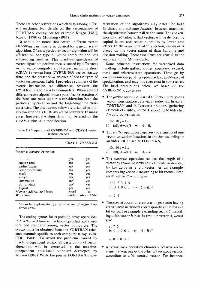
Since the invention of high-speed digital computers roughly 40 years ago, there has been a continued dramatic increase in computational power, as evi- denced by Fig. 2 (Buzbee et al., 1980). Today's fastest computers can execute hundreds of MFLOPs (mil- lions of floating-point operations per second). There are currently many new machines in the planning stages which will continue this trend, with several machines having GFLOP (giga-FLOP) capabilities announced for 1985-1990 introduction. These gains are important to scientific and engineering appli- cations because higher computing speed allows the solution of larger and more detailed problems in reasonable amounts of computer time. Alternatively, more realistic and detailed physical models may be

274 F.B. BROWN and W. R. MARTIN
10 9
%.. ,o8 I
105 /, ,030
10 3 S~c~
x~ ~ . . . . . ~ - - B : e 22(1" e't/20) ' t :0 at 1943 a,n 102
101 a/~Account lng / I Mochines
lo o • | I I I I I I I I 1940 1950 1960 1970 1980
Fig. 2. Trend in execution bandwidth of high-performance computers.
incorporated into existing codes to provide even greater precision within a given execution time.
The large increases in computation speed are due to advances in both computer hardware and computer architecture. One particular architecture results in a technique, pipelining, which is the major distinguish- ing feature of a relatively new class of machines called vector computers (Kogge, 1981). In the sections below, brief discussions are presented of vector computers in general, the modelling of vector computer instruction timing, general capabilities of the CRAY-I and CYBER-205, and programming considerations for vector computers.
1.2.1. Basic concepts. Flynn (1972) proposed a scheme for classifying computer architectures accord- ing to the relationship between instruction and data streams. Flynn included SISD (single instruction stream/single data stream), SIMD (single instruction stream/multiple data stream), MIMD (multiple in- struction stream/multiple data stream) and other classes. A conventional computer belongs to the SISD class. Instructions are executed one by one, and a single instruction deals with at most a single data operation (e.g. an addition). A SIMD machine permits instructions which can trigger a larger number of identical data operations on different data. Machines in this category may be further subdivided into parallel, in which processing units are replicated, or pipelined, in which processing units are segmented. Vector computers such as the CRAY-1 and CYBER-205 are considered pipelined SIMD ma- chines. MIMD machines are essentially a set of
processors, each with its own instruction and data streams, operating concurrently under the supervision of a master control unit. They may also be subdivided into parallel or pipelined categories. MIMD machines are currently the subject of considerable development work and may have important applications to Monte Carlo calculations in the near future.
Vector computers of the pipelined SIMD class achieve their high processing rates through the heavy use of pipelining, concurrency, chained operations, and banked and interleaved memory, each of which is discussed briefly below (Kogge, 1981; Calahan, 1980a).
Pipelining is exemplified by an automobile produc- tion line, where a number of automobiles are in production concurrently, each in a different stage of completion. The time interval between the completion of successive automobiles is equal to the time for one stage of the assembly line, rather than the total time needed to traverse the entire line. Pipelined vector computers execute instructions in a similar fashion. A functional unit is segmented, or "unrolled," into nearly independent subtasks. A stream of data operands (comprising vectors) marches in lockstep through the unit, with successive operands undergoing successive sub-tasks. The first result is obtained only after a pair of input operands traverses the entire pipeline, with successive results produced only one cycle apart. The execution of a pipelined vector instruction thus has two phases, a smrtup phase, where the pipeline is filled and the first result is obtained, and a streaming phase, where results are produced rapidly and separated only by the small delays of a segment. Pipelined architec- tures are very fast and efficient if the data stream is sufficiently large to amortize the startup times, but provide penalties in the form of startup overhead for short data streams.
Concurrency of operations, or overlap, occurs when operations involving independent data and functional units may proceed essentially simultaneously. Vector computers like the CRAY-1 and CYBER-205 allow the concurrent execution of vector and scalar instruc- tions, thus making scalar operations 'free' if they can be scheduled during a longer vector operation. The CRAY-1 also allows concurrent vector operations if no conflicts are involved.
Chaining of vector operations, also called short- stopping and linked-triads, refers to the routing of output results from one pipelined functional unit directly into the input of another, without first returning to main memory or a temporary vector register. If successive vector operations are suitable for this linking, and if a number of machine-dependent requirements are met, significant savings in startup
Monte Carlo methods on vector computers
time are realized, as well as considerable overlap of instruction execution.
Memory bankin9 and interleavin9 techniques are used to increase data transfer rates between main memory and the vector processing units. These techniques extend the parallel and pipeline techniques to memory accessing. Typically, the main memory storage is segmented into independent banks such that each bank can begin a memory cycle before adjacent banks have completed previously initiated cycles. Interleaving refers to the placement of successive data items in different banks, so that vectors of contiguous data may be transferred at high rates.
1.2.2. Vector instruction timin 9 model. The execu- tion of a vector instruction consists of a startup phase followed by a high streaming rate. For a given type of vector instruction, the timing may be modelled in a straightforward way by the formula
T(i) = S(i) + L/R (i)
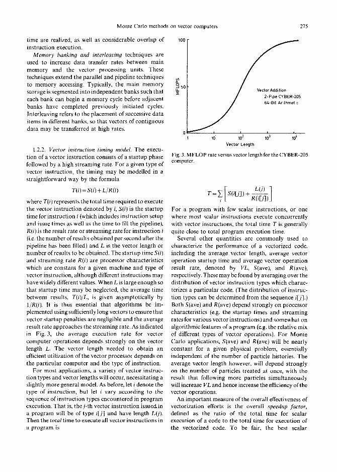
where T(i) represents the total time required to execute the vector instruction denoted by i, S(i) is the startup time for instruction i (which includes instruction setup and issue times as well as the time to fill the pipeline), R(i) is the result rate or streaming rate for instruction i (i.e. the number of results obtained per second after the pipeline has been filled) and L is the vector length or number of results to be obtained. The startup time S(i) and streaming rate R(i) are processor characteristics which are constant for a given machine and type of vector instruction, although different instructions may have widely different values. When L is large enough so that startup time may be neglected, the average time between results, T(i)/L, is given asymptotically by 1/R(i). It is thus essential that algorithms be im- plemented using sufficiently long vectors to ensure that vector startup penalties are negligible and the average result rate approaches the streaming rate. As indicated in Fig. 3, the average execution rate for vector computer operations depends strongly on the vector length L. The vector length needed to obtain an efficient utilization of the vector processor depends on the particular computer and the type of instruction.
For most applications, a variety of vector instruc- tion types and vector lengths will occur, necessitating a slightly more general model. As before, let i denote the type of instruction, but let i vary according to the sequence of instruction types encountered in program execution. That is, thej-th vector instruction issued, in a program will be of type i[j] and have length L0). Then the total time to execute all vector instructions in a program is
275
100
/ 2- Pipe CY BER-205
101 102 103 10 ~ Vector Length
Fig. 3. M F L O P rate versus vector length for the CYBER-205 computer.
R(i~j])J
For a program with few scalar instructions, or one where most scalar instructions execute concurrently with vector instructions, the total time T is generally quite close to total program execution time.
Several other quantities are commonly used to characterize the performance of a vectorized code, including the average vector length, average vector operation startup time and average vector operation result rate, denoted by VL, S(ave), and R(ave), respectively. These may be found by averaging over the distribution of vector instruction types which charac- terizes a particular code. (The distribution of instruc- tion types can be determined from the sequence i[j].) Both S(ave) and R(ave) depend strongly on processor characteristics (e.g. the startup times and streaming rates for various vector instructions) and somewhat on algorithmic features of a program (e.g. the relative mix of different types of vector operations). For Monte Carlo applications, S(ave) and R(ave) will be nearly constant for a given physical problem, essentially independent of the number of particle histories. The average vector length however, will depend strongly on the number of particles treated at once, with the result that following more particles simultaneously will increase VL and hence increase the efficiency of the vector operations.
An important measure of the overall effectiveness of vectorization efforts is the overall speedup factor, defined as the ratio of the total time for scalar execution of a code to the total time for execution of the vectorized code. To be fair, the best scalar

276 F.B. BROWN and W. R. MARTIN
algorithm should be compared with the best vector- ized algorithm, since frequently there are great differ- ences between optimal code for the two cases. It is generally meaningless to compare a vectorized al- gorithm run in scalar mode with the same algorithm run in vector mode, since vectorized code often has extra computations which need not be performed in an optimized scalar algorithm.
1.2.3. CRAY-1 and CYBER-205 overview. The CRAY-1 (Cray, 1979) is both a fast scalar and a pipelined vector processor, with a heavily integrated combination of scalar and vector instructions and registers for both applications. The basic clock period governing the entire system is 12.5 nsec. A unique feature is the presence of eight vector registers, each holding 64 words of 64 bits each. Vectors are loaded from memory into vector registers and then stream to one of 12 independent segmented functional units, with result vectors returned to vector registers. Scalar operations may proceed concurrently with all vector operations. Main memory consists of up to four million 64-bit words. Vectors consisting of either contiguous data or data separated by a constant stride may be loaded into vector registers. The allowance for a stride (which may be negative) permits easy manipu- lation of rows, columns, and diagonals of matrices. The CRAY-1 vector instructions are characterized by relatively short startup times, ranging from 25 to 175 nsec, and typical result rates of up to 80 MFLOPs, with 160 possible if two functional units are active either separately or chained. Vector opera- tions on vectors having length greater than 64 must be broken into smaller vectors. (This is done by the FORTRAN compiler automatically (Cray, 1978).i The CRAY-1 has no hardware capabilities for gather/ scatter operations or compress/expand operations (see the next section). The lack of these operations makes it necessary to use scalar instructions for creating vectors from randomly stored data or manipulating sparse data.
The CYBER-205 (CDC, 1980a,b) consists of a fast scalar processor and a multiple-pipe memory-to- memory vector processor. Both the scalar and vector processors are heavily pipelined for instruction fetch- ing and decoding, data operand fetching, and instruc- tion execution. The basic machine cycle time is 20 nsec. Startup times for the CYBER-205 vector instructions are typically 1000 nsec, but vectors reside in memory (contiguously) and may be any length up to 65,535 words. The CYBER-205 main memory is typically two million words with two vector pipes or four million words with four vector pipes. Additionally, the CYBER-205 supports very large virtual memory
capacity through the use of paging hardware which is transparent to user programs. For most vector instruc- tions, the result rates are proportional to the number of vector processing pipelines. In a vector addition on a two-pipe machine, for example, the first pipe adds the odd pairs of operands while the second pipe simul- taneously adds the even pairs, thus giving an average of one result every 10 nanoseconds. Linked triads, involving operations of the type
vector • (scalar + vector) or
vector + (scalar • vector),
may be chained together without intermediate storage of temporary results. This reduces vector startup penalties and doubles result rates. A powerful non- numeric feature of the CYBER-205 is the bit vector capabilities. For decision making operations in vector coding, hardware and addressing are provided for bit vectors, with single bits representing 'true' (1) or 'false' (0) conditions, respectively. The bit vectors may be used for logical operations, as control vectors for selective storing of results, and for manipulation of sparse vectors. Microcoded vector macroinstructions that dynamically reconfigure the vector pipes provide direct vector implementation of dot products, sum- mation of vector elements, and many other useful functions not available on the CRAY-1. Additionally, a hardware instruction is provided for vector square root operations. For forming vectors from random data or storing vector elements randomly according to an index list, the CYBER-205 has gather/scatter vector instructions, which execute in 25 nsec per data item when data are randomly distributed in memory. Compress, expand, mask, and merge vector instruc- tions facilitate the vectorized manipulation of data under bit-control. All of these operations are discussed in more detail in the following section.
1.2.4. Programming considerations. The notion of computing in a vector fashion is easily grasped by anyone who has dealt with FORTRAN programs making use of arrays and DO-loops. In general, DO- loops containing array references are directly vectoriz- able if the following things are not present :
• IF statements • GO TO statements • recursive operations • array subscripts which do not change by a constant
increment on each pass through the loop • subroutine calls • contraction of an array to a scalar quantity
(accumulation or dot product)
Monte Carlo methods on vector computers 277
There are other restrictions which vary among differ- ent machines. For details on the vectorization of F O R T R A N coding, see for example Kogge (1981), Kascic (1979) or Mossberg (1981).
It should be noted that several different vector algorithms can usually be devised for a given scalar algorithm. Often, a particular vector algorithm will be efficient on one type of vector computer and less efficient on another. This machine-dependence of vector algorithm performance is caused by differences in the vector computer architecture, including short (CRAY-1) versus long (CYBER-205) vector startup time, and the presence or absence of certain types of vector instructions. Table 1 provides a summary of the vector instruction set differences between the CYBER-205 and CRAY-1 computers. When several different vector algorithms are possible, the selection of the 'best' one must take into consideration both the particular application and the target-machine char- acteristics. The discussions below are oriented prima- rily toward the CYBER-205 vector computer. In many cases, however, the algorithms may be used on the CRAY-I with little modification.
Table 1. Comparison of CYBER-205 and CRAY-1 vector instruction sets
CRAY-1 CYBER-205
Vector Hardware Operations
+, - ,*,/ yes yes square root no yes gather/scatter no yes compress/expand no yes mask yes yes merge no yes summation no a yes dot product no a yes logical yes yes
Memory Addressing Modes word bit Word Size 64-bit 64- or 32-bit
a=can be implemented by recursive use of vector func- tional units.
The coding syntax for expressing array operations in a vectorized form is machine-dependent and there- fore not standard among vector computers. The syntax must be obtained from the F O R T R A N refer- ence manuals specific to each computer (Cray, 1978; CDC, 1980c). To avoid the problems caused by machine-dependent syntax, all descriptions of vector algorithms will be presented in the machine- independent notational standard developed by Iverson (1962). While the precise F O R T R A N imple-
mentation of the algorithms may differ (for both hardware and software features) between machines, the algorithmic features will be the same. The conven- tion adopted below is that vectors will be denoted by capital letters and scalar quantities by lower case letters. In the remainder of this section, emphasis is placed on the vectorization of data handling and decision making. These two items are crucial to the vectorization of Monte Carlo.
Some principal instructions for vectorized data handling include gather, scatter, compress, expand, mask, and selective-store operations. These go by various names, depending upon machine and degree of specialization, and may not even exist in some cases. The brief descriptions below are based on the CYBER-205 architecture.
• The 9ather operation is used to form a contiguous vector from random data via an index list. In scalar F O R T R A N and in Iverson's notation, gathering elements of B into a vector A according to index list I would be written as
Do 10 j = 1,n 10 (ai) j))=b(j) ,~ A ~ B ,
• The scatter operation disperses the elements of one vector to random locations in another according to an index list. In scalar F O R T R A N ,
Do 10 j = l,n 10 a(l( j ) )=b(j) ¢¢, A t . - B
• The compress operation reduces the length of a vector by removing unwanted elements, as denoted by the zeros in a bit vector. As an example, compressing vector A according to bit vector B into result vector C would give:
a : 1 2 3 4 5 b:O 1 0 0 1 ¢~, C ~ B / A
c : 2 5
• The expand operation creates a longer vector having zeros placed in elements corresponding to zeros in a bit vector. For example, expanding vector C accord- ing to bit vector B into the result in vector A, would give
c : 2 5 b: 0 1 0 0 1 ~ A , -B ~C
a : 0 2 0 0 5
• A vector mask operation chooses successive vector elements from one or the other of two input vectors, according to a bit control vector. For instance,

278 F.B. BROWN and W. R. MARTIN
given input vectors A1 and A2 and bit vector B, a mask operation may select from A 1 for '1' bits in B or A2 for '0" bits in B to form result vector C:
a 1 : 1 2 3 4 a 2 : 5 6 7 8 <:~ C~-- /A2 ,B ,A1/
b: 0 0 1 1
c: 5 6 3 4
• A vector merge operation combines features of the mask and expand operations. Given input vectors A1 and A2 and bit vector B, a merge operation will select the next unused element of A 1 or A2. That is, merging A1 (for '1' bits in B) with A2 (for '0' bits in B) gives a result vector C as:
a 1 : 1 2 3 4 a 2 : 5 6 7 b: 1 1 1 0 0 1 ¢~, C ~ \ A 2 , B , A I \
c: 1 2 3 5 6 4
• A reduct ion operation is applied recursively to successive elements of a vector to produce a single scalar result. The reduction operation for addition, for example, is equivalent to a summation of the successive elements of a vector:
a : 1 3 5 7 s = ( ( ( 1 ) + 3 ) + 5 ) + 7 .¢~ s . + / A
• A bit count operation is a special case of the reduction operator and determines the number of ' l ' bits in a logical bit vector. For example,
b : 1 0 0 1 1 1 n = 4 ¢~, n~- + / B
• A vector length operation returns the current length of a vector. Its inverse operation may be used to set the vector length to a given value.
a: 1 2 3 4 5 .¢~ s~VL(A) s = 5
Decision making in a vectorized calculation is generally handled either by using extra computation followed by a vector mask or by rearranging al- gorithms to place conditional statements (e.g. IF statements) outside the vector code. As a typical example, consider the scalar FORTRAN coding
Do 10 j = l ,n
xU)=0.0 10 if 0c(j).gt.0.0) x(j)= 1.+ y(j)
Each pass through the loop involves a choice between two values depending on the result of a comparison. In a vectorized calculation, the decision process must be
completed before vector X enters a vector pipeline. This might be vectorized as:
B~ F > 0 T, 1.+Y
x ~ - /O,B,T/
Each of the vector operations above could be carried out as a single vector instruction. Note that 1. + Y0") is computed for all elements, rather than only the necessary ones. This extra work will (in this case) be offset by the much higher computation rates obtained from the vector mode calculations. In general, any two-way decision may be vectorized by computing both possible results and then selecting the correct one by using the masking operation.
Short independent segments of coding may often be vectorized syntactically in a straightforward manner by programmers. The vectorization of a large, complex production code, however, requires the re- examination of many interrelated kernels and data structures and cannot in general be achieved effectively without major algorithm changes. This consideration is the topic of the next section.
2. VECTORIZED MONTE CARLO~GENERAL
[n developing new methods for solving large-scale problems on state-of-the-art computers, engineers and scientists should no longer think strictly in terms of equations and then depend on clever programmers or optimizing compilers to efficiently solve their prob- lems. Vector processing takes advantage of data structure, takes a 'larger view', in order to gain parallelism and enhance processing rates. This larger view is not available to compilers or pure pro- grammers due to the basic character of the program development process. In going from theory to equa- tions to algorithms to flow charts to conventional coding, the original problem is progressively trans- formed in a way that is not syntactically reversible. The larger view of the problem is lost. Considering the significant advantages of vectorization, the message is clear that although codes can be 'vectorized', the big payoffs come from vectorizing algorithms (Brown, 1981a; Owens, 1973; Remund and Taggart, 1977; Smz, 1980; Wirsching and Kishi, 1977).
After an overview of previous work in vectorizing Monte Carlo, a larger view of the Monte Carlo method will be taken to determine what structure exists. It will be shown that despite the random behavior of individual particles, vectorized global algorithms are readily formulated for treating sets of particles. The implementation of these algorithms, the 'vectorization'
Monte Carlo methods on vector computers 279
of the coding, is later discussed in Section 3, with numerical examples presented in Section 4.
2.1. Previous work
The first known work related to vectorizing Monte Carlo is that of Troubetzkoy et al. (1973), who adapted a version of the continuous-energy code SAM-CE for use on the ILLIAC-IV. The ILLIAC-IV was an experimental parallel SIMD processor with 64 pro- cessing elements. The basic approach was to follow a number of histories in each processing element, performing a given computation such as tracking only if 'enough' processing elements had at least one particle each waiting for that operation. Those processing elements without waiting particles were disabled for that operation. In essence, this approach mimics MIMD operation on a parallel SIMD machine by means of 'turning off' unwanted processing elements, and is not suitable for vector processors. The basic technique of forming queues of particles according to the type of next event, however, was developed. This technique is used (in some form) in all current vectorized Monte Carlo codes. The estimated overall efficiency was about 30~,,, leading to an estimated speedup of 20 over the conventional machines of the time. Since the ILLIAC-IV was under development and unavailable, Troubetzkoy's predictions were de- rived from simulation on a standard scalar computer.
Recent efforts to vectorize Monte Carlo were initiated in 1979 by discussions between T.L. Jordan of LANL and D.A. Calahan of the University of Michigan. Jordan produced two codes--a scalar version and a vectorized version--which were sent to Michigan for further study and optimization by D.A. Catahan et al. (Calahan et al., 1980b,c; Brown et al., 1981d,e). These codes and their succeeding develop- ment are discussed briefly below.
A very short (300 lines) and simple scalar Monte Carlo code for the continuous-energy transport of gamma-rays served as a starting point for vectorized Monte Carlo investigations. In this code, a 6 MeV pencil-beam source was incident upon a single cylinder of carbon, with three collision interactions treated between 0.001 and 20 MeV. Compton scattering, pair production, and photo-electric absorption were in- cluded. No secondary particles were allowed (pair production was treated by emitting a particle with double weight), no variance reduction schemes were included, only analog absorption was permitted, and tallies were made with no variance calculation. This 'bare-bones' Monte Carlo code was intended purely
for basic algorithmic studies, and not for comparison with production-level codes.
The initial attempt to vectorize the code, i.e. to follow many particles simultaneously, was implemen- ted using a particle stack comprised of vectors containing weight, energy, position, and direction components of all currently active particles. The particle stack was initially filled with values obtained from a starting source routine. A table search was performed to look up particle cross-sections which were then interpolated on particle energy. Then all particles were tracked simultaneously. Since only one geometric cell was permitted in the problem geometry, vectorization of the coding for particle tracking was straightforward. Only a few algorithmic changes were needed. Since there was only one cell, particles either collided within the cell or crossed the outer boundary. Particles crossing the cell boundary were tallied and deleted from the stack. For the remainder of the stack, the type of collision was sampled for each particle using the previously computed cross-sections, and particles were sorted into queues for either Compton scatter, pair production, or termination by absorption. Each interaction was vectorized in a straightforward manner to process the appropriate queue of particles. The direction and energy of the secondary particles due to Compton scattering and pair production were sampled from the appropriate PDF's and the particle stack was suitably modified. After deleting captured particles and performing a few tallies, the particle stack was topped off with source particles, and the entire process was repeated. The major algorithmic feature of this code relevant to vectorization is that each random decision point in the Monte Carlo procedure results in sorting particles into queues for vectorized analysis followed by a merging of results back into the particle stack. The key to the algorithm is the fundamental similarity of all particle interactions---each is initiated by particle emission at a given phase space position (source or collision) and proceeds to termination (collision or boundary crossing). Defining this portion of a particle history as an 'event' (emission through termination), the vectorized algorithm may be des- cribed as an 'event-based' algorithm versus the con- ventional 'history-based' algorithms of scalar Monte Carlo codes.
To study a slightly more general geometry, the carbon cylinder was divided into several concentric cylinders. All particles, regardless of location, were tracked simultaneously by finding the distances to every surface in the cylinder. Particles crossing a cell boundary were stopped and merged with source particles for the next iteration. Since all cells were logically the same, only minor changes were needed in

280 F.B. BROWN and W. R. MARTlY
the particle tracking routine. For tallying purposes, an extra array was used to hold the cell number for each particle.
In an alternative attempt to generalize the geometric treatment, a cell-by-cell approach was used. The major algorithm change involved treating particles within a single cell simultaneously, with an outer iteration over cells. To accomplish this, a separate particle stack was maintained for each cell. Particles in the current cell which crossed a cell boundary were transferred to the particle stack for the 'other-side' cell. Particles collid- ing inside the current cell were queued up for the collision physics routines, and then merged back into the current stack after collision analysis. Although this code permitted only a concentric cylinder geometry, the algorithm was later extended in the MCVMG code to a more general geometry.
Variance estimation was added via the batching method (RSIC, 1977). To implement batching, an outer loop was added so that a batch of particles was processed to completion before starting another batch. The batch mean scores are thus statistically indepen- dent estimates of the true mean and are used to estimate the variance. The introduction of batching has no effect on the coding of the random-walk, and thus introduced no changes in vectorized kernels.
Details of the coding and algorithmic characteristics of the above codes can be found in Calahan et al. (1980b,c) for the CRAY-1 implementation, and Brown et al. (198 ld, e) and Martin (1983a) for the CYBER-205 implementation. The speedups due to vectorization in these initial studies were in the range of 5 10 times faster than the original scalar code. While these speedups are relatively modest, the systematic investi- gation of new algorithms formed the basis for more recent efforts (the MCVMG code at the University of Michigan and the MCV code at KAPL) which have attained measured speedups of 20 85 for practical problems.
The next sections describe this work in more detail. It should be noted that there are alternative ap- proaches to vectorizing Monte Carlo in addition to the approach considered in this paper. Bobrowicz et al. (1983) have vectorized a photon transport Monte Carlo code for the CRAY-1, wherein each distinct process is assigned to a separate queue and the queue is "executed" only when it is full (length 64) or if it is the longest queue when all are less than 64 in length. This approach is more suitable for the CRAY- 1 (which does not have vector hardware capabilities for gather/scat- ter or compress/expand) than are the CYBER-205- oriented methods used in MCV and MCVMG. Bobrowicz et al. report speedups of 7-10 over an optimized CRAY-1 scalar coce. (Speedups relative to a
CDC-7600 version of the code are indicated to be in the range of 20-35.) Martin (1983b) has reported preliminary results of an independent effort to vector- ize a photon transport Monte Carlo code for inertial confinement fusion applications. Speedups on the CRAY-I were in the range of 7 10 relative to an optimized CDC-7600 code.
2.2. General considerations for vectorized Monte Carlo
In order to achieve large speedups from vectoriz- ation, some restructuring of the global Monte Carlo algorithms is necessary. While there are no 'typical' Monte Carlo problems, there do exist may similar- ities in structure among the many existing production codes. All general-purpose Monte Carlo codes include the following major computational kernels:
• introduction of particles from a source. • retrieval of cross-sections from an extensive data
base (multigroup or continuous-energy) • sampling the distance to collision. • tracking of particles in general geometry, including
determination of the distance to the next surface crossing, identification of the next surface, and identification of the next or current cell.
• determining the particle energy and direction fol- lowing collisions from discrete and/or continuous PDF's.
• determination of secondar) particle production (if applicable), and resulting energy and direction.
• tallying to estimate means and variances. • miscellaneous variance and cost reduction tech-
niques such as splitting/Russian roulette, weight cutoffs, etc.
The above kernels are implemented in most general- purpose codes in roughly the same manner. Since each of the kernels is relatively seff-contained and straight- forward there are many similarities among the general- purpose codes. Conventional scalar Monte Carlo codes may be characterized as a collection of loosely coupled computational kernels, with individual par- ticle histories simulated one-at-a-time by random sampling to select a kernel and by further random sampling within individual kernels. The vectorized Monte Carlo codes are formulated computationally to follow many particles through their random-walks, treating many events simultaneously using vector instructions to speed up the computation rates. Syntactic (i.e. local) vectorization of a scalar Monte Carlo code is not effective since different particles would require analysis by different kernels. Instead, experience has shown that a comprehensive, highly

Monte Carlo methods
integrated approach is required to achiek~e significant gains in computational efficiency. The m~ajor elements of the computational structure that efficiently pro- cesses many particles simultaneously are noted as follows:
(1) The Monte Carlo code must access a unified data layout. The entire cross-section and geometry database must be restructured to provide the unffied data layout. For a given portion of the calculation, the data should be memory-resident and organized so that simple and logical direct addressing may be used to facilitate vector gather operations.
(2) The Monte Carlo code must be restructured (re- written). Much rearrangement of local coding and the global algorithm is required to permit the processing of many particles simultaneously. Large amounts of memory storage must be allocated to hold the descriptive data for each particle. These data are 'stacked' in memory so that corresponding components form vectors. The global algorithm used to manage the particle stack and to vectorize across random decision points is described in detail below in the discussion of implicit loops.
(3) Deliberate and careful code development is essential. Scalar Monte Carlo production codes are large and complex and have evolved gradually over many years of development. Vectorized Monte Carlo codes must accommodate the additional complexity of managing the storage and shuffling of thousands of particles simultaneously. Development should begin with small codes having few options. As methods are verified and experience is accumulated, additional options and capabilities may be systematically added.
The key to successful vectorization of Monte Carlo is that a well-defined structure must be imposed on both the database and Monte Carlo algorithm before coding is attempted. This structure may arise simply from the reorganization of existing data/algorithms or may entail the development of special mathematics or physics models. Careful and systematic development helps to preserve the structure as the vectorized code becomes more complex.
2.3. Vectorization techniques
The principal obstacle to vectorizing a conventional scalar Monte Carlo code is the large number of conditional statements ( I F . . . GO TO) contained in
on vector computers 281
the coding. Examination of sections of coding shows that, typically, one-third of all essential FORTRAN statements may be IF-tests. Careful consideration of the Monte Carlo program logic and underlying physics permits categorizing these conditional state- ments and associating them with three general al- gorithmic features of Monte Carlo code~ imp l i c i t loops, conditional coding and optional coding. The techniques used in vectorizing each of these features are discussed below. As noted previously, the primary emphasis is on techniques applicable to the CYBER-205 vector architecture.
2.3.1. Implicit loops. Monte Carlo codes have a notable absence of explicitly stated DO loops. The most heavily used loops are implicit. That is, they generally do not have a loop counter, and the number of iterations may not be fixed or known in advance. Termination is based upon the setting of some condition within the loop. Some examples are the implicit free-flight loop (i.e. track and move a particle repeatedly until it collides) and the implicit loop on particle termination (i.e. simulate particle free-flight and collisions until the particle escapes or is absorbed). Implicit loops generally occur in the global logic of a Monte Carlo code or in the specific coding for random sampling via rejection methods. I f . . . GOTO state- ments that branch backward in the coding are quite often the terminators of implicit loops. (In a structured programming language, implicit loops would be implemented via DO-WHILE structures.)
In the global logic, the end of an implicit loop is a transition between loosely connected sections of coding, such as tracking vs. collision analysis. In a vectorized algorithm, some particles being analyzed may (physically) exit the implicit loop on the first pass while others may require many passes. One general technique for resolving this difficulty will be termed 'shuffling'. At the end of each pass through an implicit loop, the particle data are shuffled. Particles that have satisfied the exit condition are transferred to a storage queue (i.e. a 'stack') to be held until all particles have satisfied the exit condition of the implicit loop. Particles that have not satisfied the exit condition are left in the working stack for the implicit loop. The working stack is then compressed so that contiguous vectors are available for the next pass through the implicit loop. The implicit loop terminates when its working stack is empty. (In some cases, there may be advantages to terminating the implicit loop early and saving its stack for later use.)
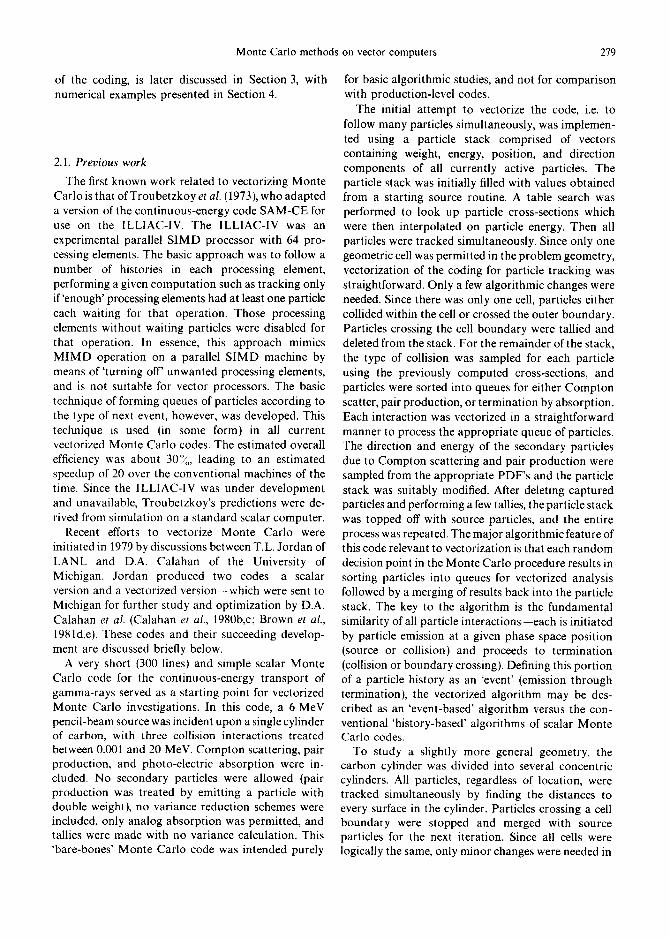
The use of shuffling in vectorized Monte Carlo is illustrated in Fig. 4 (Brown, 1983) which shows the global algorithm and neutron stacks for MCV. Due to
282 F.B. BRowN and W. R. MARTIN
Batch Loop
Source
Supergroup Loop
Shuffle
Collision Loop
Free-fllght Loop
. . . . Track
. . . . Shuffle
C o l l i s i o n s
S h u f f l e o , °
, ° .
Track ~XY Z • . .
Collide x Y z . . .
Bank XYZ
Fig. 4. Global algorithm and neutron stacks for vectorized continuous-energy reactor lattice analysis.
the very large size of the detailed pointwise cross- section dataset, the energy range is segmented into distinct nonoverlapping ranges called 'supergroups', with the random-walk completed in one supergroup before proceeding to the next. The implicit loops are the collision loop and the free-flight loop. In the free- flight loop, all neutrons are tracked simultaneously, regardless of their geometric location. At the end of the free-flight loop, neutrons may remain in the tracking stack or be transferred to the collision stack. At the end of the collision loop, neutrons may be transferred to the tracking stack or to the bank stack (if the energy after collision falls outside the energy range of the
current supergroup). The shuffle just prior to the collision loop is used to retrieve banked neutrons at the start of a new supergroup.
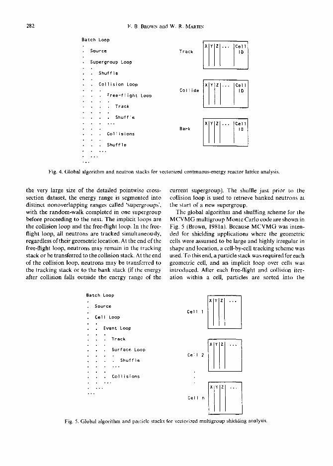
The global algorithm and shuffling scheme for the MCVMG multigroup Monte Carlo code are shown in Fig. 5 (Brown, 1981a). Because MCVMG was inten- ded for shielding applications where the geometric cells were assumed to be large and highly irregular in shape and location, a cell-by-cell tracking scheme was used. To this end, a particle stack was required for each geometric cell, and an implicit loop over cells was introduced. After each free-flight and collision iter- ation within a cell, particles are sorted into the
Batch Loop
Source
Cell Loop
Event Loop
Track
Surface Loop
. . . . S h u f f l e
Collisions , , .
. , o
celjxYiZl ...
ce121xLYiz Cell n l X Y Z ...
Fig. 5. Global algorithm and particle stacks for vectorized multigroup shielding analysis.
Monte Carlo methods on vector computers 283
appropriate stacks for other cells. Since relatively compact multigroup cross-section data were used, no shuffling was needed for energy group consider- ations--all collisions could be treated simultaneously.
2.3.2. Conditional codino. The physical laws of particle behavior are simulated in a Monte Carlo code by random sampling from probability distributions. The outcome of random sampling determines the next event in a neutron history. For a scalar code, an I F . . . GOTO statement is used to test a condition and to branch (usually forward) to an appropriate section of coding. Sections of coding that are either selected or skipped, depending upon some particle attribute, will be termed conditional coding. (In a structured pro- gramming language, conditional coding would be implemented via CASE structures.)
Conditional coding occurs often in the most frequently used portions of the Monte Carlo al- gorithm. In vectorized Monte Carlo, some particles in the current stack must undergo a particular set of operations (such as inelastic scattering), while others must not undergo these operations. Shuffling would generally introduce too much overhead and degrade performance. Instead, selective operations must be performed when vectorizing conditional coding. Four different means of performing selective operations on the CYBER-205 are described here and illustrated by examples in following sections.
1. Gather/operate/scatte~Data for the selected par- ticles are transferred from random stack locations into contiguous vectors using vector gather instruc- tions. The necessary operations are then performed, and results are scattered back into the proper positions in the particle stack. Data for particles not selected remain in the stack unaffected.
4.
2. Compress~operate~decompress--This is similar to gather/operate/scatter, but uses compress and de- compress vector operations. Gather/scatter is more efficient when selected data are sparse; compress/ decompress is more efficient when selected data are dense.
3. Bit-controlled operations--For short conditional coding blocks, the overhead from gather/scatter or compress/decompress may be greater than the gains from vectorization. These cases may be vectorized using the CYBER-205 bit-controlled operation capability. A vector operation is per- formed on all the elements of a vector, with results stored only for elements corresponding to a per- missive bit in a bit vector.
Generalized equations--Much of the conditional coding in scalar Monte Carlo codes is included to save time for simple or specialized cases. As an example, isotropic scattering is a special case of general scattering analysis and is usually treated separately by simplified equations. In a vectorized code, it is very often more efficient to avoid separate coding for special cases and, instead, to use general equations for all particles. This should be done whenever it appears that the extra work resulting from the use of general equations is less than the overhead of gather/scatter or compress/decompress operations needed for separate analysis. In general, this tradeoff will depend on the specific machine architecture as well as on the particular coding.
2.3.3. Optional codin 9. Monte Carlo codes permit many input options that specify the type of calculation to be performed. These options select or skip sections of coding for all particles and need no special treatment in a vectorized code. For example, a neutron eigenvalue problem must include operations for deter- mining the source shape used in succeeding batches, whereas a fixed-source problem utilizes a known source shape. One simple branch in a vectorized code will skip unneeded operations for all particles. This provides an important speedup over a scalar code where the branch is needed for each particle.
2.3.4. Discussion. To summarize, implicit loops are vectorized using shuffling, and conditional coding is vectorized using selective operations. This approach to vectorizing Monte Carlo is effective on the CYBER-205 and other vector computers having hardware capabilities for vectorized data handling. In the MCVMG and MCV vectorized Monte Carlo codes, 40 60~/o of all vector instructions used in actual coding were vector data handling instructions (gather, compress, bit-controlled operations, etc.).
The data-handling operations associated with shuf- fling and selective operations in the vectorized code constitute extra work that is not necessary in a scalar code. This extra work offsets some of the gain in speed achieved from vectorization. For vectorization to be successful, overhead from shuffling and selective operations should comprise only a small fraction of total computing time. It is thus essential that all data handling operations be performed with vector instruc- tions. Vector computers that rely on scalar data handling operations are severely limited in vectorized Monte Carlo performance.

284 F.B. BROWN and W. R. MARTIN
3. VECTORIZED MONTE CARLO~SPEC1FIC
Where the previous section discussed the vectoriz- ation of Monte Carlo in general terms, this section presents specific examples of vectorizing localized portions of a Monte Carlo code. The examples have been taken from either the MCVMG code, a vector- ized multigroup Monte Carlo demonstration code, or from the MCV code, a vectorized continuous-energy neutron transport Monte Carlo code for reactor analysis.
3.1. Pseudorandom number generation
The 'randomness' in a Monte Carlo calculation stems from randomly sampling probability distribu- tions which model physical events. On digital com- puters, pseudorandom number generators ((PRNG's) are used to supply ' random' numbers uniformly distributed in the interval 0-1. While PRNG's make use of deterministic algorithms and hence do not yield truly random numbers, the sequences produced by PRNG's will pass suitable tests for randomness when the algorithm parameters are chosen correctly. Although PRNG's account for only about 5!!/, or less of the total CPU time for a typical Monte Carlo calculation, the vectorization of PRNG's is important to avoid 'scalar bottlenecks' in a highly vectorized code. (That is, if the remainder of the coding were completely vectorized, the maximum speedup would be less than 20.)
The most common PRNG used in scalar Monte Carlo for radiation transport applications is the multiplicative congruential method (or Lehmer method) (Halton, 1970; Knuth, 1981). A sequence of pseudorandom integers s(i) is generated according to:
s(0),--initial integer seed
~ + 1),--gs(i) mod p (1)
The integers s(i), termed seeds, are in the range (1 ,p- 1). The modulus p is generally chosen to be 2", where m is the number of binary digits used to represent a positive integer. If the generator g is chosen so that g(mod 8)=3 or 5, then the sequence will have the maximal length of 2"-2 without repeating. (The initial seed s(0) must be odd to prevent the sequence from degenerating to repeated zeros.) The pseudoran- dom numbers on (0,1) produced by s(i)/p are used in sampling from the probability distributions which model a particle's physical behavior in a Monte Carlo code.
Although the scalar PRNG Algorithm (1) is recur-
sive, it may be vectorized in a straightforward way by either 'unrolling' or 'replicating' the recursion. Unrolling leads to a 'vector seed, scalar generator' algorithm, while replication leads to a 'scalar seed, vector generator' algorithm, both of which are des- cribed below. These vectorized algorithms preserve the exact sequence defined by the scalar algorithm (1).
The 'vector seed, scalar generator' (VSSG) al- gorithm for generating vectors having L pseudoran- dom numbers is obtained by unrolling the recursion of Algorithm (1) L times. In this scheme, vector S(k) will contain the (kL+ 1) through (kL+L) elements of the pseudorandom sequence produced by Algorithm (1). The initial seed vector S(0) is generated using the scalar algorithm, while successive seed vectors are produced using vector hardware instructions. The seed vectors must be retained in memory for the next pass.
S(O)~(s(O), s(1) . . . . . s(L- 1))
S(k T 1)~gLS(k) rood p (2)
/
The 'scalar seed, vector generator' (SSVG) al- gorithm for generating vectors having L pseudoran- dom components discards the seed vector S(k + 1 ) after it is used, retaining only the last element as the scalar seed for the next pass. A vector consisting of the generator g to successive powers is used in generating the next seed vector S(k+ 1). The generator vector is computed only once and retained without change throughout the calculation.
s(0),--initial scalar seed
G~(g , g2 . . . . . gL)mod p
1 S(k+ 1 ) ~ G s(k) rood p (3)
s(~+ 1)* [S(k+ 1)] L
/
While the VSSG and SSVG schemes are mathemat- ically equivalent and preserve the pseudorandom sequence of Algorithm (1), practical considerations favor the SSVG algorithm for general-purpose use. For Monte Carlo applications such as radiation transport where the vector length L varies during the calculation, the VSSG algorithm is inefficient due to the need to generate a new seed vector S(0) using scalar methods whenever L changes. The SSVG algorithm is preferable since it will accommodate varying L values if the generator vector is initialized for the largest required value of L. Although L may vary, the elements of G remain constant.
Monte Carlo methods on vector computers 285
The SSVG algorithm is currently implemented in the MCVMG vectorized Monte Carlo code for the CYBER-205 computer. Initialization of G is per- formed once at the start of a problem using scalar instructions. The generation of S(k+ 1) in Algorithm (3) and conversion to a vector of normalized fractions R(k+ I) require only three vector hardware instruc- tions, resulting in an asymptotic timing of 30 nsec per pseudorandom vector element (for a 2-pipe CYBER-205). This timing is more than an order of magnitude faster than scalar implementations (which have measured timings of about 320 nsec).
Recently, more general PRNG algorithms have been proposed by Frederickson et al. (1983) in which the initial seeds are chosen by means of a separate PRNG. Frederickson presents convincing arguments for the adoption of these new algorithms.
3.2. Sampling direction cosines
As an example of vectorizing a short, localized
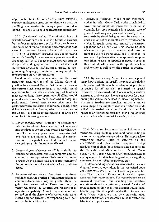
portion of a Monte Carlo code, consider part of the process of sampling a direction from an isotropic angular distribution. It is necessary to evaluate cos~b and sin~b, where ~b is an angle uniformly distributed on (0,2re). Figure 6 shows several schemes for this process. The direct (scalar) calculation (Fig. 6a) is straight- forward but somewhat slow, due to the need to evaluate the trigonometric functions. The rejection method (Fig. 6b) for indirect sampling of sintk and cos~b is faster, since it avoids the use of the SIN and COS functions, and is the method used in nearly all Monte Carlo codes (Carter and Cashwell, 1975). lf i t is desired to produce many pairs of samples at once, the process should be vectorized. The rejection method cannot be readily vectorized, however, due to the conditional branch ( I F . . . GO TO statement). Vectorizing the direct calculation (Fig. 6c) is possible and leads to the production of pairs of results 5.5 times faster than via rejection, and 9 times faster than via scalar computation, even though the trigonometric functions are being evaluated. Such savings are
6a. D i r e c t Method IScalar)
R = 2 . *PI~RANF (1) u = COS (R) V = SIN(R)
T i m i n g " (microseconds) Amdahl 4 7 0 v / 8 17. CRAY-1 8 . 4 CYBER-205 9 .1
6b . Rejection Method / S c a l a r )
10 R1 = 2 . *RANF(1 ) - 1. R2 = 2.*RANF(1) - 1. T = R1,~2 + R2~.2 IF ( T .GT. 1 .0 ) GO TO 10
T = ] . / T U = ( R 1 * ~ 2 - R 2 * * 2 ) * T V ~ 2 . ~ R I ~ R 2 * T
Timing* (microseconds) Amdahl h7Ov/8 12. CRAY-I 5 .2 CYBER-205 3 .0
6c. V e c t o r i z e d D i r e c t Method
DO 10 I = I . N Timing" (microseconds) R( f ) = 2 .~PI~RANF(1) (per pa i r of r e s u l t s ) U(I ) = C O S ( R ( I ) ) Amdahl h70v /8 17. V ( I ) = S I N ( R ( I ) ) CRAY-1 .94
10 CONTINUE CYBER-205 -57
* CRAY-1 and CYBER-205: 6~ b i t a r i t h m e t i c , Amdahl 4 7 O v / 8 : 3 2 b i t a r i t h m e t i c
Fig. 6. Local vectorization example.

286 F.B. BROWN and W. R. MARTIN
important in repetitive and often used parts of a larger calculation.
The above discussion brings out two important programming considerations: First, repetitive calcula- tions involving trigonometric, exponential, or arith- metic functions may often be coded simply and directly due to efficient vectorized functions. It is not (always) necessary to use rejection methods or other tricks common in scalar codes. Less arithmetic does not necessarily mean faster code on a vector computer. Extra arithmetic needed to allow vectorization can very often result in faster overall code.
3.3. Rejection methods
Rejection methods are frequently used for random sampling from complicated probability distributions. In a scalar code, a rejected trial sample leads to a (backward) branch in order to repeat the sampling process. In a vector code, provision must be made for separating the accepted and rejected trials resulting from the sampling process. These methods may be vectorized through a shuffling procedure--accepted trials are appended or intermixed with previously accepted ones, and the necessary parameters of the rejected trials are collected together before repeating the sampling process. The overhead for the shuffling of accepted and rejected samples comprises extra work required for vectorization which is not present in scalar coding. Since these methods are often employed in frequently used portions of coding, the overhead from shuffling is an important consideration. In some cases, the additional work is minimal and does not significantly degrade performance. For many rejection sampling schemes involving only a few simple opera- tions, however, the amount of 'algorithmic overhead' required for vectorization will often outweigh the gains from vectorization. It is preferable to replace rejection methods by direct methods wherever possible, even for sampling from complicated probability density functions.
3.4. Russian roulette vectorization example
As a final example of vectorizing a short localized segment of a Monte Carlo code, a Russian roulette procedure common to most Monte Carlo codes will be considered. This procedure is used to kill off particles having low weight in order to reduce the total computing time. In order to avoid biasing the results, particles with low weight are killed off probabilistic- ally, with the weight of survivors increased so that the expected weight is preserved. Figure 7a illustrates this process as coded in FORTRAN in a typical scalar
code. First, a test is made to see if particle weight is below the weight cut-off criteria. If so, the particle survives with probability (wgt/wrrave), where wgt is the particle weight and wrrave is the weight assigned to surviving particles. If the particle survives it is given a weight of wrrave; if not, it is terminated by setting the weight to zero. Vectorization of the Russian roulette game to permit many particles to play at once is simplified if the coding of Fig. 7a is first rewritten in the equivalent structured form shown in Fig. 7b, where FORTRAN block-IF structures have been used to eliminate GO TO statements. For many particles at once, the coding of Fig. 7c must be made compatible with vector processing instructions by eliminating the IF-slatements. To illustrate the tradeoffs involved in deciding between possible vector implementations, three different approaches are illustrated in Figs 7d--f along with examples of the instruction timings taken from the CYBER-205.
Figure 7d illustrates the vectorization of the Russian roulette process through the use of vector mask instructions, without the use of compress/expand or gather/scatter operations. In this approach, bit vectors are formed based on both tests found in the scalar method, and then two vector masks are used to place either 0, wrrave, or the original particle weights into the appropriate vector element positions. The disad- vantage to this approach is that extra work must be performed (compared to scalar), since a random number is generated for all particles rather than just for the ones having low weight.
Figure 7e illustrates one method to avoid the extra work of unnecessary random number generation. Using the initial bit vector (which flags the particles having low weight), the weights and random number seeds of particles which must undergo Russian roulette are compressed into shorter vectors. The Russian roulette process is then played only for those particles, and then the results are expanded back into the appropriate positions in the original vectors. There is thus some overhead due to the compress/expand operations, but the random process itself is played only for the particles which may be affected by it. Based on the CYBER-205 timings shown in Figs 7d and 7e (and neglecting vector startup times), this approach is faster than the vector mask approach when the number of particles which must undergo Russian roulette is less than about 31/60 of the original number of particles.
Figure 7f illustrates another method of playing the Russian roulette game only on affected particles. In this approach, the initial bit vector (which flags particles with low weight) is used to create a vector containing the indices of affected particles (with respect to the start of the original vector). Using the
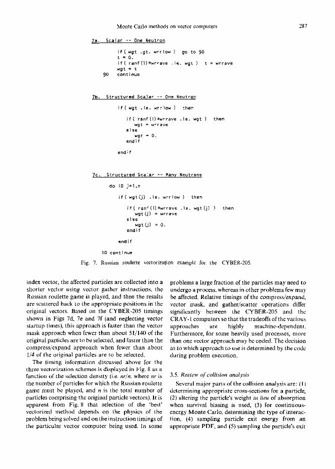
Monte Carlo methods on vector computers 287
]a. Scalar - - One Neutron
9O
i f ( wgt .gt . wrrlow ) go to 90 t : O . i f ( ranf(1)*wrrave . le . wgt ) t = wrrave wgt = t cont i hue
7b. Structured Scalar - - One Neutron
i f ( wgt . le . wrrlow ) then
i f ( ranf(1)*wrrave . ]e . wgt ) wgt = wrrave
else wgt = O.
endif
endif
then
7 c. Structured Scalar - - Many Neutrons
do I0 j=l,n
if(wgt(j) .le. wrrlow ) then
if( ranf(l)*wrrave .le. wgt(j) ) wgt(j) = wrrave
else wgt (j) = O.
endlf
e n d i f
10 continue
Fig. 7. Russian roulette vectorizalion example for the
then
CYBER-205.
index vector, the affected particles are collected into a shorter vector using vector gather instructions, the Russian roulette game is played, and then the results are scattered back to the appropriate positions in the original vectors. Based on the CYBER-205 timings shown in Figs 7d, 7e and 7f (and neglecting vector startup times), this approach is faster than the vector mask approach when fewer than about 51/140 of the original particles are to be selected, and faster than the compress/expand approach when fewer than about 1/4 of the original particles are to be selected.
The timing information discussed above for the three vectorization schemes is displayed in Fig. 8 as a function of the selection density (i.e. nr/n, where nr is the number of particles for which the Russian roulette game must be played, and n is the total number of particles comprising the original particle vectors). It is apparent from Fig. 8 that selection of the 'best' vectorized method depends on the physics of the problem being solved and on the instruction timings of the particular vector computer being used. In some
problems a large fraction of the particles may need to undergo a process, whereas in other problems few may be affected. Relative timings of the compress/expand, vector mask, and gather/scatter operations differ significantly between the CYBER-205 and the CRAY-1 computers so that the tradeoffs of the various approaches are highly machine-dependent. Furthermore, for some heavily used processes, more than one vector approach may be coded. The decision as to which approach to use is determined by the code during problem execution.
3.5. Review of collision analysis
Several major parts of the collision analysis are: (1) determining appropriate cross-sections for a particle, (2) altering the particle's weight in lieu of absorption when survival biasing is used, (3) for continuous- energy Monte Carlo, determining the type of interac- tion, (4) sampling particle exit energy from an appropriate PDF, and (5) sampling the particle's exit
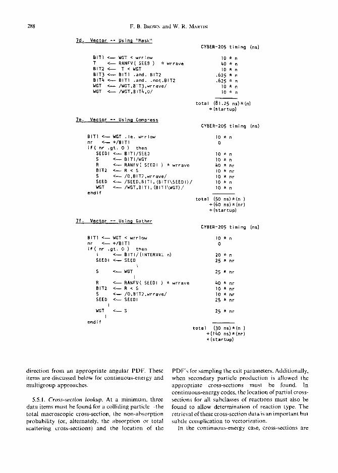
288 F.B. BROWN and W. R. MARTIN
7d. Vector - - Using "Mask"
BIT1 < - - WGT < wrrlow T < - - RANFV( SEED ) ~ wrrave BIT2 < - - T < WGT BIT3 < - - BITI .and. BIT2 BIT4 < - - BIT1 . and . . no t .B IT2 WGT < - - /WGT,BlT3,wrrave/ WGT < - - /WGT,BIT4,O/
7~. Vector -- Using Compress
BITI < ~ WGT . l e . wrrlow nr < ~ +/BITI i f ( nr .g t . O ) then
SEEDI < - - BITI/SEED S < - - BITI/WGT R < - - RANFV( SEEDI ) * wrrave BIT2 < - - R < S S < - - /O,BIT2,wrrave/ SEED < - - /SEED,BITI,(BITI\SEEDI)/ WGT < ~ /WGT,BITI,(BITI\WGT)/
end i f
7 f . Vector - - Using Gather
BIT1 < - - WGT < wrrlow nr < - - +/B~TI i f ( nr .g t . O ) then
I <-- BITI/(INTERVAL n)
SEEDI < - - SEED I
S <-- WGT
I R <-- RANFV( SEEDI ) * wrrave BIT2 < - - R < S S <-- /O,BIT2,wrrave/ SEED < - - SEEDI
I WGT <-- S
I e n d i f
CYBER-205 t iming (ns)
1 0 . n 4 0 * n 1 0 ~ n
• 625 ~ n • 625 * n
IO* n
I0" n
t o t a l (81.25 n s ) * ( n ) + (s ta r tup)
CYBER-205 timing (ns)
1 0 , n 0
1 0 , n 10 ~. n 40 * nr
IO *, nr
IO * nr
IO* n
IO* n
t o t a l (50 n s ) * ( n ) + (60 n s ) * ( n r ) + (s ta r tup)
CYBER-205 t i m i n g (ns)
10 ~ n 0
2 0 r a n 25 * nr
25 * nr
40 * nr 10 * nr 10 * nr 25 * nr
25 ~ nr
t o t a l (30 ns) m(n ) +(140 ns) * (nr) + ( s ta r tup)
direction from an appropriate angular PDF. These items are discussed below for continuous-energy and multigroup approaches.
5.5.1. Cross-section lookup. At a minimum, three data items must be found for a colliding particle--the total macroscopic cross-section, the non-absorption probability (or, alternately, the absorption or total scattering cross-sections) and the location of the
PDF's for sampling the exit parameters. Additionally, when secondary particle production is allowed the appropriate cross-sections must be found. In continuous-energy codes, the location of partial cross- sections for all subclasses of reactions must also be found to allow determination of reaction type. The retrieval of these cross-section data is an important but subtle complication to vectorization.
In the continuous-energy case, cross-sections are
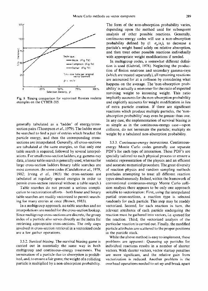
Monte Carlo methods on vector computers 289
e
/ o°
io°°° °°**°'°°°°*~-~ ~ ~ '~ ~ ~ ~ ~ ~
125
100
u ~75
~s0
o.,° , , ~ ' ~ Technique:
~ / / / - - M a s k (Fig 7d) ~mCompress (Fig 7e)
• " ...... Gather (Fig 7f) o," Tin = ave. time per original
vector element p = nrln
I I I l
25*/, 50*/, 75"/, 100'/, Selection Density, p
Fig. 8. Timing comparison for vectorized Russian roulette examples on the CYBER-205.
generally tabulated as a 'ladder' of energy/cross- section pairs (Thompson et al., 1979). The ladder must be searched to find a pair of entries which bracket the particle energy, and then the corresponding cross- sections are interpolated. Generally, all cross-sections are tabulated at the same energies, so that only one table search is required, followed by several interpol- ations. For small cross-section ladders, e.g. gamma-ray data, a linear table search is generally used, whereas for large cross-section ladders binary table searches are most common. (In some codes (Candelore et al., 1978, 1982; Irving et al., 1965) the cross-sections are tabulated at regularly spaced energies in order to permit cross-section retrieval without a table search.)
Table searches do not present a serious compli- cation to vectorization efforts--both linear and binary table searches are readily vectorized to permit search- ing for many entries at once (Brown, 1983).
In a multigroup approach, no table searches and no interpolations are needed for the cross-section lookup. Since multigroup cross-sections are discrete, the group index of a particle also serves directly as the index for retrieving appropriate cross-sections. The only steps involved in cross-section retrieval in a vectorized code are a few gather operations.
3.5.2. Survival biasing. The survival biasing game is carried out in essentially the same way in both multigroup and continuous-energy treatments. The termination of a particle due to absorption is prohib- ited, and, to ensure a fair game, the weight of a colliding particle is multiplied by a non-absorption probability.
The form of the non-absorption probability varies, depending upon the method used for subsequent analysis of other possible reactions. Generally, continuous-energy codes will use a non-absorption probability defined by (1--O'a/fit), to decrease a particle's weight based solely on relative absorption, and then treat other possible reactions individually with appropriate weight modifications if needed.
In multigroup codes, a somewhat different defini- tion is used (Gabriel, 1978). Neglecting the produc- tion of fission neutrons and secondary gamma-rays (which are treated separately), all remaining reactions are accounted for at a collision by considering what happens on the average. The 'non-absorption prob- ability' is actually a misnomer for the ratio of expected surviving weight to incoming weight. This ratio implicitly accounts for the non-absorption probability and explicitly accounts for weight modification in lieu of extra particle creation. If there are significant reactions which produce multiple particles, the 'non- absorption probability' may even be greater than one. In any case, the implementation of survival biasing is as simple as in the continuous-energy case--upon collision, do not terminate the particle; multiply its weight by a tabulated non-absorption probability.
3.5.3. Continuous-energy interactions. Continuous- energy Monte Carlo codes generally use separate PDF's for each type of interaction. These PDF's are specially tailored to each physical process to ensure a realistic representation of the physics and an efficient and accurate numerical procedure. The great diversity of reaction physics and random sampling methods precludes attempting to treat all different reaction types simultaneously. Indeed, within the framework of conventional continuous-energy Monte Carlo colli- sion analysis there appears to be only one approach suitable to vectorization : First, using the interpolated partial cross-sections, a reaction type is selected randomly for each particle. This step may be readily vectorized. Second, for each reaction in turn, the relevant attributes of each particle undergoing the reaction must be gathered into vectors, i.e. queued for the reaction. Third, the vectorized analysis of the particular reaction is carried out. Finally, the modified particle attributes are scattered to the proper positions in the particle stack.
While the above method is easy to implement, these problems are apparent: Queueing up particles for individual reactions results in a number of shorter vectors. With shorter vectors, vector startup penalties are more significant, and the relative gain from vectorization is reduced. Another problem is the overhead operations needed to set up and break apart

290 F.B. BROWN and W. R. MARTIN
vector queues. The penalties from these extra opera- tions may somewhat offset gains from the vectorized collision analysis. Despite these problems, vectorized continuous-energy collision analysis has been found to be very effective in the MCV code. Brown (1983) details the techniques used to vectorize the collision analysis at epithermal energies in MCV. The types of interactions considered include elastic scattering (iso- tropic, P1, PN,), inelastic scattering, and a modified free-gas model to treat epithermal scattering with hydrogen bound in water.
3.5.4. Multigroup collision analysis. The compli- cations occurring with continuous-energy collision analysis are absent from the multigroup approach. Since all reactions are averaged together in forming the group-to-group transfer matrix, only one type of PDF is necessary to sample the exit group for each particle--the discrete P D F represented by one column of the transfer matrix. Thus, no queueing or sorting of particles for separate interactions is required. A similar situation exists with regard to PDF's related to the scattering angle. The multigroup cross-section pro- cessing codes can average together the angular distri- butions of all reactions, and, although various codes make use of different representations, a given code will represent the angular PDF's in one way. Many of the methods used for representing angular PDF's for multigroup cross-sections have been summarized by Brockman (1981). The two most commonly used are the representation of scattering densities in the form of equiprobable step function PDF's (Carter and Forest, 1976) and in the form of moment-preserving discrete angles. Both of these forms are suitable for vectorization.
The key requirement for vectorizing the multigroup collision analysis is the vectorization of random sampling from discrete PDF's. A method for vectoriz- ing discrete sampling has been developed by Brown et al. (1981c, 1983). The new vectorized discrete sampling method has been found to be equivalent to the 'aliasing' method of Walker (1977) and is a particular extension of Marsaglia's (1961) method as applied to discrete distributions. It is faster than the usual method for sampling discrete distributions with large table length N, executes in a fixed time independent of N, and can be efficiently implemented into Monte Carlo codes for parallel and vector processing computers. The new vectorized method is significantly faster than all scalar methods and executes in a fixed time regardless of the size of the distribution. This new discrete sampling method is used for all discrete sampling events in the MCV and MCVMG codes.
3.6. Vectorization of tracking
Despite the great number of schemes for tracking particles through general geometry, most tracking modules in Monte Carlo codes can be loosely categor- ized as either 'COMJOM' or 'surface-segment' ap- proaches. The COMJOM (combinatorial geometry) approach originated for the SAM-CE code, has been adopted and extended in MORSE and KENO, and generalized for MCNP. The surface-segment ap- proach has been used in the ANDY series of codes and in many older codes. In the following sections, the similarities of all tracking schemes in a simple geo- metry are discussed, followed by a general comparison of the COMJOM and the surface-segment approaches to complex geometry. The surface-segment tracking scheme was used in the vectorized MCVMG code, while a simplified version of the COMJOM scheme was used in the MCV code.
3.6.1. Basic tracking considerations. The basic descrip- tion of problem geometry is conveyed to a Monte Carlo code through the coefficients of equations for surfaces and through lists defining relations between cells (or regions) and surfaces. Each surface compris- ing the problem geometry is described by a linear or quadratic equation (or for special tori, simplified fourth order equations) of the form S(x,y,z)= 0. In the most general case, the surface equation is
S(x,y,z) = Ax 2 + By z + Cz 2 + Dxy + Eyz
+Fxz + G x + H y + Jz + K=O,
although most surfaces are considerably simpler in form. The distance d along the direction (u,v,w) between a given point (x',y',z') and a surface is found by solving the quadratic equation S(x'+ ud, y '+ vd, z' + wd) = 0 for d. To track a particle through a general geometry, some scheme is needed to define cells in terms of bounding surfaces and to resolve complex or ambiguous cases. The COMJOM approach is a high- level approach in that the basic building blocks are bodies. A body is a simple geometric region of space completely enclosed by quadratic surfaces such that a ray will pierce the body at only two points. Basic bodies include spheres, boxes, cylinders (with top and bottom faces), etc. Complex geometric cells can be created of course by combining bodies using intersec- tion, union, and complement operators. Input process- ing modules convert the logical combinations of bodies into distinct simple regions along with lists used for combining the simple regions. The surface-segment scheme is a low-level approach in that the infinite surfaces are subdivided into bounded surface- segments. The surface-segments are then stitched

Monte Carlo methods on vector computers 291
together explicitly to form geometric cells. In principle, either approach is sufficiently general to allow the description of geometry of any degree of complexity.
In both approaches, there are three basic items to be determined: (1) the distance to the nearest valid cell boundary, (2) identification of the boundary (e.g. an index in a list of boundary segments), and (3) identification of the cell on the other side of the boundary (i.e. the 'other-side' cell number). For particles inside the simplest of cells (bodies), these three items are found in essentially the same way by both tracking methods. For more complicated cases, additional operations are needed involving surface senses. The sense of a given poin t (x',y',z') with respect to a surface defined by S(x,y,z) =0 is generally taken as positive if the quantity S(x',y',z') is greater than zero, and negative if S(x',y',z') is less than zero. Then, for example, a point inside a sphere has a negative sense (with respect to the spherical surface), and a point outside the sphere has positive sense.
3.6.2. Distance to simple cell boundaries. The pro- cedure for determining the free-flight distance to the nearest boundary is essentially the same for all tracking methods for the case of simple cells. Given a list of the number of surfaces bounding each cell, a list of the type of surface (e.g. plane perpendicular to x-axis, sphere, etc.) and a list of the location in memory of the surface coefficients, it is a simple matter to loop over the surfaces of a cell, finding the roots of the appropriate linear or quadratic equation to determine distances to the surfaces. For simple cells, the smallest positive distance so calculated is the desired quantity. No surface sense information is needed.
Vectorization of tracking in simple cells is relatively straightforward when a cell-by-cell global algorithm is used. Considering vectors containing position and direction components of each particle in a given cell, an outer loop is made over the surfaces bounding the cell. For each surface, the roots of the surface equation are found simultaneously for each particle in the cell stack using vector arithmetic. The smallest positive root and the index of the corresponding surface are retained for each particle using simple vectorized relational operations.
Vectorization of tracking in simple cells is more complicated when it is desired to simultaneously track particles which may be in different cells. First, an index vector must be formed to identify the particular equation to be solved for each particle. The appro- priate equation coefficients must then be gathered into contiguous vectors. In general, the logic is simplified if a general quadratic equation is used,
rather than, for example, using simplified linear equations for plane surfaces.
A minor complication arises over the treatment of particles having complex roots for the distance calcu- lation. For the quadratic case, a negative discriminant in the quadratic formula indicates the roots will be complex, while a zero discriminant indicates a multiple root. Both of these cases should be discarded, since complex roots correspond to no intersection and equal roots correspond to a tangent intersection. In a scalar code, when a negative or zero discriminant occurs, a branch is made to skip further calculation for that surface-segment. In a vectorized calculation, con- ditional branches cannot be made for individual particles. Two alternatives are possible: first, at various points in the coding where some particles fail a test, the particle vectors could be compressed and the calculation continued. At the end, after a number of intermediate steps and compressions, the results would have to be expanded back to the proper positions. Alternatively, no compression or expansion would be used, but rather dummy results would be substituted into the particle vectors in such a way that the final logic tests would fail for the particles in question. Either approach involves extra work, either in compression/expansion or in unneeded calcula- tions. The substitution of dummy results for some particles failing a test was the approach used in the MCV and MCVMG codes.
3.7. Tallying considerations
The tallying of particle scores is the only significant facet of the Monte Carlo random-walk which has not been vectorized in MCV and MCVMG. Nevertheless, the tally process is markedly affected by the approach to vectorization used in the rest of the code. Brief discussions of significant considerations for tallying are given below.
3.7.1. Scalar versus vectorized tallyin 9. The most basic sequence of operations involved in tallying the scores for many particles is a loop of the form:
Do 10 j = 1,N 10 r(iO))=r(i(j))+s(j)
where N is the number of particles, sO) is the score for thej-th particle, i(j) is an index identifying the tally bin to which so.) contributes and r is an array of tally bins for accumulating overall scores (e.g. reaction rates). This type of tally operation will generally be performed for every type of event that particles undergo. A tracklength estimate of cell group fluxes is made after tracking operations by summing the products of
292 F.B. BROWN and W. R. MARTIN
particle weights times free-flight track lengths into the appropriate group bins. If collisions occur, particle weights are summed into the appropriate group bins for collision estimators of cell fluxes (after eventual division by the total cross-sections). If boundary crossings occur, particle weights are summed into the appropriate bins for surface crossing estimators of partial currents across surface-segments. (Some codes do not provide boundary crossing estimators,)
Only a few tally loops of the form shown above are needed within the vectorized random-walk. As dis- cussed below, most other scoring operations can be moved outside of the random-walk. The tallying loops shown above have been found to comprise only about 1% of the operations in MCVMG and MCV and thus have very little effect on the overall code performance. These loops have been carefully 'fine-tuned' using hand-optimized scalar coding.
The cell fluxes and partial currents are usually not the only information desired from a calculation. In general it is necessary to fold a cross-section or response function into the flux or current to obtain an integral quantity such as total absorption or dose rate. For continuous-energy calculations, this can be per- formed after the random-walk if all cross-sections are tabulated on the same energy mesh. If interpolation laws are to be used for the cross-sections, additional information may need to be tallied during the random- walk analysis. For example, the use of a linear cross- section interpolation law in post-editing requires that both flux and energy*flux be tallied on each collision or free-flight. The price paid for the advantage of post- editing is the increased storage required to accumulate group fluxes and partial currents for every cell and energy interval. This storage is not large compared to that needed for the particle stacks, but does contribute to total memory usage.
3.7.2. Batchin 9 method for variance calculation. The variance of tallied scores is estimated in MCV and MCVMG via the batching method (McGrath et al., 1975; RSIC, 1977). That is, a problem is divided into independent batches of particles, and the variance is computed from the RMS deviation of batch scores from the overall mean. Direct computation of variance through the tallying of squared particle scores is not practical for a vectorized calculation due to the excessive storage required to accumulate partial scores associated with each independent source particle. (Allowance for splitting would create further compli- cations.) The batching method, in contrast, is easier to implement and is better suited to vector calculations since it is simply an outer loop in the calculation.
4. NUMERICAL STUDIES
This section details the numerical studies performed on the CYBER-205 in support of the discussions in previous sections. The specific objectives of these numerical studies have included verification of the validity (correctness) of the codes and algorithms, determination of performance characteristics of the vectorized codes for several practical problems, and comparison with optimized scalar codes of similar capabilities to determine the relative gains achieved by vectorization.
4.1. Capabilities of MCVMG
The MCVMG code is a vectorized multigroup Monte Carlo demonstration code. This code in- corporates the most significant physics and algor- ithmic features of standard production codes without a plethora of user conveniences and options. MCVMG is a CYBER-205 code utilizing the FORTRAN explicit vector syntax. A scalar code, MCS (Brown, 1981a), written in FORTRAN, has identical capabilities but makes full use of all time-saving techniques used in conventional scalar Monte Carlo codes. MCS pro- vides a representative scalar benchmark for timing comparisons for the vectorized code. Multigroup Monte Carlo speedups due to vectorization are determined by comparing execution times for prob- lems run using the scalar MCS code and the vector MCVMG code.
Both scalar and vector codes have identical capa- bilities and physical models chosen selectively from typical general-purpose production codes such as MORSE, KENO, ANDY and MCNP. The specific capabilities include: (a) The description of problem geometry utilizes the
surface-segment scheme with unique other-side cells. Currently, the geometric surface types al- lowed include planes perpendicular to the x, y, or z axes, planes of arbitrary orientation, cylinders parallel to the x,y, or z axes, and spheres. (Other linear or quadratic surface type could easily be added without complications.) Any number of cells, surfaces, and surface-segments may be speci- fied, with storage for the particle stacks (in MCVMG) being the constraint on problem size, rather than the geometric description. Any planar surface-segment may be flagged as a reflecting, periodic, or non-reentrant boundary.
(b) Tallies are made for the group fluxes in every cell and the partial currents (positive and negative) across each surface-segment. The cell fluxes may be estimated using either tracklength or collision estimators. Response functions may be included in
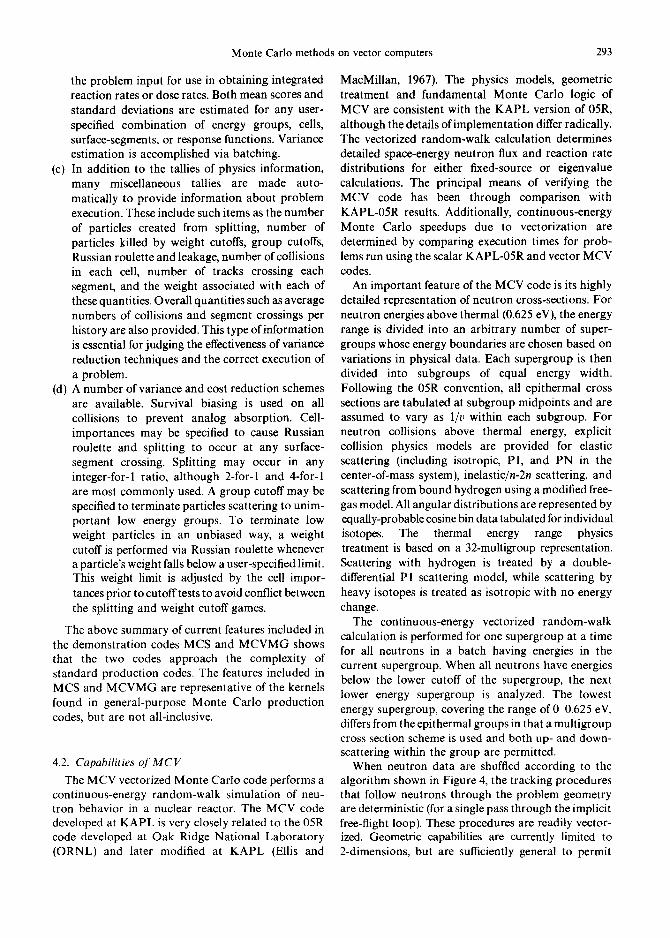
Monte Carlo methods on vector computers 293
the problem input for use in obtaining integrated reaction rates or dose rates. Both mean scores and standard deviations are estimated for any user- specified combination of energy groups, cells, surface-segments, or response functions. Variance estimation is accomplished via batching.
(c) In addition to the tallies of physics information, many miscellaneous tallies are made auto- matically to provide information about problem execution. These include such items as the number of particles created from splitting, number of particles killed by weight cutoffs, group cutoffs, Russian roulette and leakage, number of collisions in each cell, number of tracks crossing each segment, and the weight associated with each of these quantities. Overall quantities such as average numbers of collisions and segment crossings per history are also provided. This type of information is essential for judging the effectiveness of variance reduction techniques and the correct execution of a problem.
(d) A number of variance and cost reduction schemes are available. Survival biasing is used on all collisions to prevent analog absorption. Cell- importances may be specified to cause Russian roulette and splitting to occur at any surface- segment crossing. Splitting may occur in any integer-for-1 ratio, although 2-for-1 and 4-for-1 are most commonly used. A group cutoff may be specified to terminate particles scattering to unim- portant low energy groups. To terminate low weight particles in an unbiased way, a weight cutoff is performed via Russian roulette whenever a particle's weight falls below a user-specified limit. This weight limit is adjusted by the cell impor- tances prior to cutofftests to avoid conflict between the splitting and weight cutoff games.
The above summary of current features included in the demonstration codes MCS and MCVMG shows that the two codes approach the complexity of standard production codes. The features included in MCS and MCVMG are representative of the kernels found in general-purpose Monte Carlo production codes, but are not all-inclusive.
4.2. Capabilities of MCV The MCV vectorized Monte Carlo code performs a
continuous-energy random-walk simulation of neu- tron behavior in a nuclear reactor. The MCV code developed at KAPL is very closely related to the 05R code developed at Oak Ridge National Laboratory (ORNL) and later modified at KAPL (Ellis and
MacMillan, 1967). The physics models, geometric treatment and fundamental Monte Carlo logic of MCV are consistent with the KAPL version of 05R, although the details of implementation differ radically. The vectorized random-walk calculation determines detailed space-energy neutron flux and reaction rate distributions for either fixed-source or eigenvalue calculations. The principal means of verifying the MCV code has been through comparison with KAPL-05R results. Additionally, continuous-energy Monte Carlo speedups due to vectorization are determined by comparing execution times for prob- lems run using the scalar KAPL-05R and vector MCV codes.
An important feature of the MCV code is its highly detailed representation of neutron cross-sections. For neutron energies above thermal (0.625 eV), the energy range is divided into an arbitrary number of super- groups whose energy boundaries are chosen based on variations in physical data. Each supergroup is then divided into subgroups of equal energy width. Following the 05R convention, all epithermal cross sections are tabulated at subgroup midpoints and are assumed to vary as 1/v within each subgroup. For neutron collisions above thermal energy, explicit collision physics models are provided for elastic scattering (including isotropic, P1, and PN in the center-of-mass system), inelastic/n-2n scattering, and scattering from bound hydrogen using a modified free- gas model. All angular distributions are represented by equally-probable cosine bin data tabulated for individual isotopes. The thermal energy range physics treatment is based on a 32-multigroup representation. Scattering with hydrogen is treated by a double- differential P1 scattering model, while scattering by heavy isotopes is treated as isotropic with no energy change.
The continuous-energy vectorized random-walk calculation is performed for one supergroup at a time for all neutrons in a batch having energies in the current supergroup. When all neutrons have energies below the lower cutoff of the supergroup, the next lower energy supergroup is analyzed. The lowest energy supergroup, covering the range of 00.625 eV, differs from the epithermal groups in that a multigroup cross section scheme is used and both up- and down- scattering within the group are permitted.
When neutron data are shuffled according to the algorithm shown in Figure 4, the tracking procedures that follow neutrons through the problem geometry are deterministic (for a single pass through the implicit free-flight loop). These procedures are readily vector- ized. Geometric capabilities are currently limited to 2-dimensions, but are sufficiently general to permit
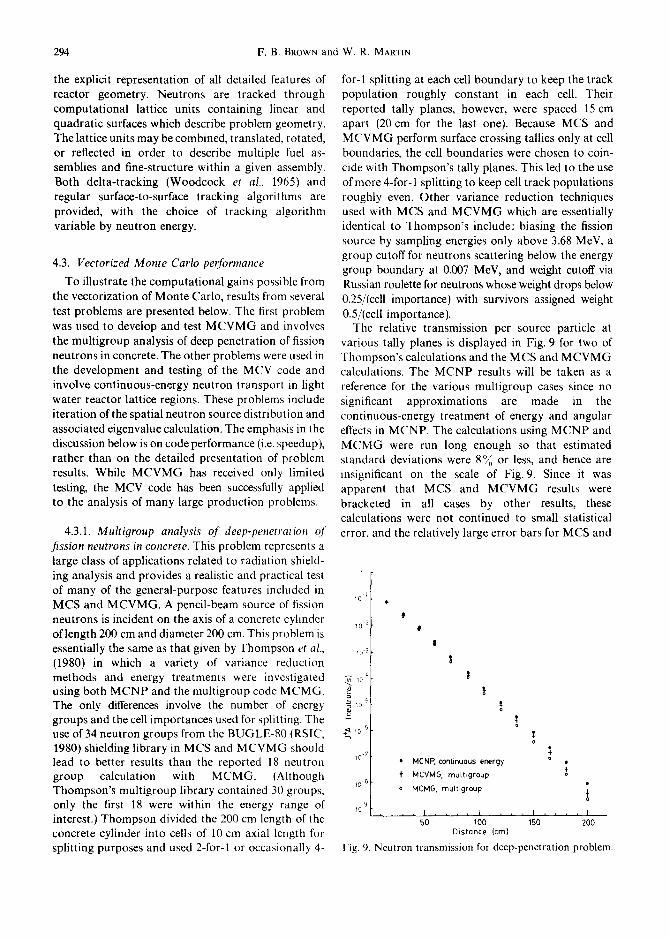
294 F.B. BROWN and W. R. MARTIN
the explicit representation of all detailed features of reactor geometry. Neutrons are tracked through computational lattice units containing linear and quadratic surfaces which describe problem geometry. The lattice units may be combined, translated, rotated, or reflected in order to describe multiple fuel as- semblies and fine-structure within a given assembly. Both delta-tracking (Woodcock et al., 1965) and regular surface-to-surface tracking algorithms are provided, with the choice of tracking algorithm variable by neutron energy.
4.3. Vectorized Monte Carlo performance
To illustrate the computational gains possible from the vectorization of Monte Carlo, results from several test problems are presented below. The first problem was used to develop and test MCVMG and involves the multigroup analysis of deep penetration of fission neutrons in concrete. The other problems were used in the development and testing of the MCV code and involve continuous-energy neutron transport in light water reactor lattice regions. These problems include iteration of the spatial neutron source distribution and associated eigenvalue calculation. The emphasis in the discussion below is on code performance (i.e. speedup), rather than on the detailed presentation of problem results. While MCVMG has received only limited testing, the MCV code has been successfully applied to the analysis of many large production problems.
4.3.1. Multigroup analysis o f deep-penetration qf .fission neutrons in concrete. This problem represents a large class of applications related to radiation shield- ing analysis and provides a realistic and practical test of many of the general-purpose features included in
lO -1
MCS and MCVMG. A pencil-beam source of fission neutrons is incident on the axis of a concrete cylinder l o_~ of length 200 cm and diameter 200 cm. This problem is essentially the same as that given by Thompson et al., ,o.3 (1980) in which a variety of variance reduction methods and energy treatments were investigated ~ ,0 ~ using both MCNP and the multigroup code MCMG. The only differences involve the number of energy ~ ~o' groups and the cell importances used for splitting. The - use of 34 neutron groups from the BUGLE-80 (RSIC, ÷~ ~0 s 1980) shielding library in MCS and MCVMG should
10 -7 lead to better results than the reported 18 neutron group calculation with MCMG. (Although
!0 8
Thompson's multigroup library contained 30 groups, only the first 18 were within the energy range of ~09 interest.) Thompson divided the 200 cm length of the concrete cylinder into cells of 10 cm axial length for splitting purposes and used 2-for-1 or occasionally 4-
for-1 splitting at each cell boundary to keep the track population roughly constant in each cell. Their reported tally planes, however, were spaced 15 cm apart (20 cm for the last one). Because MCS and MCVMG perform surface crossing tallies only at cell boundaries, the cell boundaries were chosen to coin- cide with Thompson's tally planes. This led to the use of more 4-for-1 splitting to keep cell track populations roughly even. Other variance reduction techniques used with MCS and MCVMG which are essentially identical to Thompson's include: biasing the fission source by sampling energies only above 3.68 MeV, a group cutoff for neutrons scattering below the energy group boundary at 0.007 MeV, and weight cutoff via Russian roulette for neutrons whose weight drops below 0.25/(cell importance) with survivors assigned weight 0.5/(cell importance).
The relative transmission per source particle at various tally planes is displayed in Fig. 9 for two of Tbompson's calculations and the MCS and MCVMG calculations. The MCNP results will be taken as a reference for the various multigroup cases since no significant approximations are made in the continuous-energy treatment of energy and angular effects in MCNP. The calculations using MCNP and MCMG were run long enough so that estimated standard deviations were 8% or less, and hence are insignificant on the scale of Fig. 9. Since it was apparent that MCS and MCVMG results were bracketed in all cases by other results, these calculations were not continued to small statistical error, and the relatively large error bars for MCS and
8,
0
!
I !
!
• M C N P , c o n t i n u o u s e n e r g y
• 1" M C V M G , m u i t i g r o u p
o M C M G , m u l t i c J r o u p
. . . . I . , , , I , ,
5 0 I 0 0
D i s t a n c e ( c m l
~t o
, I , , , , I
150 2 0 0
Fig. 9. Neutron transmission for deep-penetration problem.

Monte Carlo methods on vector computers 295
MCVMG reflect this. Additional results from Thompson et al. (1980) not shown on Fig. 9 are the 240 group calculations performed using MCNP in a pseudo-multigroup fashion. That is, reaction cross- sections were multigroup, but energy and angular scattering effects were treated by the normal continuous-energy scheme. These results lie between the MCS/MCVMG results and the MCNP results.
Consideration of the results in Fig. 9 leads to two conclusions: First, in a realistic test of MCS and MCVMG on a practical problem, the codes perform correctly and have sufficient generality to be con- sidered representative of production codes. Second, the accuracy of the multigroup approach is sensitive to the fineness of the energy group structure. The trend in going from 18 groups to 34 groups to 240 groups (with continuous-energy scattering treatment) is unar- guably toward better physics and closer agreement with a continuous-energy method.
This problem allows an assessment of the vectorized performance characteristics for a realistic applied problem, the deep-penetration of fission neutrons in concrete. This case also illustrates that standard variance reduction schemes may enhance vectorized performance. In a typical MCVMG run with 1,000 particles starting a batch, 11,786 particles were created by splitting, 4,978 particles were killed by Russian roulette, 7,029 were lost due to the group cutoff, 93 were killed in the Russian roulette weight cutoff and 714 were lost by leakage. An average particle under- went 113 collisions and crossed 14 segments.
Figure 10 provides insight into the dynamic nature of the performance characteristics by displaying the MOPs, MFLOPs, VL and total number of particles as functions of total predicted CPU time for a 2-pipe CYBER-205 using full-precision arithmetic. (These quantities were estimated by modelling the CYBER-205 instruction timings in an emulated ver- sion of MCVMG, as detailed in Brown (1981a).) Starting with a batch size of 1,000, the number of particles increases to nearly 5,000 midway through the run due to splitting. The average vector length is much smaller, however, since the particles are distributed among 14 cells. Examining MOPs, MFLOPs and VL shows that they stay relatively constant while the particle population is increasing and begin to decline only in about the last third of the calculation where particles are killed rapidly by cutoffs.
A series of calculations was performed to determine the vectorized performance characteristics as func- tions of the batch size. Measured MCVMG execution times on the CYBER-205 (2-pipe, 64-bit arithmetic) were compared to the corresponding MCS timings on the Amdahl 470V/8 to determine the speedups due to
80
60
40
20 lOPS ~ " ~ ,
5o
40
30
20
10
:F o++--., ' 5000 600 ~, e-"-"-,, Por ticles
450 ~ ~'~%, 4000
%.,---,-,.m~ 3000 300/ V L o v e ~ ~ 2000 150 , , ~ ~ ~ 1000
.I . 2 .3 .4
CPU Time (estimoted)
Fig. 10. Vectorized Monte Carlo dynamic performance on the CYBER-205 for deep-penetration problem.
vectorization. These timings vary from problem to problem and, for a given problem, fluctuate slightly due to statistical effects from the Monte Carlo analysis. Figure 11 presents MCVMG speedups for this prob- lem. The relative speedup increases rapidly with batch size at first and then reaches an asymptotic value of about 40 over the Amdah1470V/8 scalar computation. This behavior may be attributed to the effects of vector startup. For small batch size the average vector is short, and the average overhead per operation from
4 0
:o 2 0
CO
I O
~ t L l L J , , , , , , I J L I i i l l l i I
IO 2 I03 iO 4 Particles/ Batch
Fig. 11. Performance results for vectorized multigroup Monte Carlo on the CYBER-205.
296 F.B. BROWN and W. R. MARTIN
vector startup is large compared to the actual opera- tion time in streaming. For larger batch size, the vectors are longer and the efficiency is higher. That is, the effects of startup are less when averaged over the larger number of elements in longer vectors. The speedup is close to asymptotic for batch sizes of several 1,000 source particles.
Further insight is provided into problem dynamics and the effects of splitting, Russian roulette and the iteration scheme by Fig. 12. This plot shows the distribution of particles in each cell throughout the iteration process. The initial wave of source particles is seen to rapidly travel outward, being reinforced and 'herded' in the proper direction by splitting. The cells are populated rapidly and the total number of particles grows• When the wave reaches the opposite boundary, the majority of splitting has already occurred and there is then an alternation among the most populated cells which gradually spreads out as cell populations dwindle. It should be noted that secondary particle creation should produce the same type of effect as spl i t t ing~the creation of particles during the calcula- tion should increase vector lengths and enhance vectorized performance.
4.3.2. Continuous-energy vectorized Monte Carlo analysis. To verify the correctness of the vectorized MCV code and to determine the speedups due to vectorization, several benchmark problems were run (Brown, 1982) using both the scalar KAPL-05R code on the CDC-7600 and the vectorized MCV code on the
CYBER-205. These problems involved the analysis of two-dimensional light-water-reactor lattice regions having reflecting boundary conditions. The problems were run in both fixed-source and eigenvalue modes, and included either 19 or 186 geometric regions and 280 edited reaction rates. Detailed comparison of scalar and vector results showed agreement to within small statistical uncertainties (95~,,~ confidence intervals).
The speedup of Monte Carlo neutron processing rates for a typical problem is shown in Fig• 13 (Brown, 1983) as a function of the number of neutrons per batch. The vectorized code performance varies with batch size, because larger batches lead to longer average vector lengths and to reduced vector instruc- tion startup overhead. For most problems, batches of 16,000 neutrons are used to obtain problem-averaged vector lengths in the range of 500-1,000 and achieve excellent vector efficiency.
Recent development efforts (Brown and Mendelson, 1984) have concentrated on extending the generality and capabilities of MCV to permit its usein a variety of production-oriented reactor analysis applications. Examples of typical applications of the MCV code and relative speedups attained are given below for three cases which span the range of current problem sizes IBrown and Mendelson, 1984). (1) The analysis of a fuel element unit cell (fuel, clad
and water) with a fixed-source in the fuel region is a typical 'small' problem. Spatially-dependent reac- tion rates from this problem provide the basic data
Deep Penetration of Fission Neutrons in Concrete Cylinder
./
Fig. 12. Cell population ~ersus iteration for deep-penetration problem.

Monte Carlo methods on vector computers 297
3000
2500
~ 2 0 0 0
1500
10oo
50O
- - - t . . . . "~ . . . . i 1 ¢ t t 4 0 0 0 12000 8000
Neutrons/Botch
lO
16000
60
50
4 0 ~
?o g
20
Fig. 13. Performance results for vectorized continuous- energy Monte Carlo on the CYBER-205.
for constructing resonance interference and thermal self-shielding factors for use in few-group cross-section generation for diffusion theory calcu- lations. A special version of MCV has been optimized for this generic problem type. Neutron histories are processed at a rate in excess of 200,000/min, providing speedups of 75-85 times better than scalar computation using KAPL-05R on the CDC-7600.
(2) Determination of the reaction rates and eigenvalue for a collection of fuel elements in a fuel assembly constitutes a typical 'medium' sized problem. The results of such a problem are typically used to check the corresponding results of a fine-mesh few- group diffusion theory calculation. For problems involving several hundreds or thousands of spatial regions, five to ten compositions, and several hundred edited reaction rates, the MCV code processes 75,000-200,000 neutron histories per minute, giving speedups of 20-60 over scalar rates.
(3) At the present time, a 'large' problem is one which, for example, treats the depletion of a fuel assembly, including spatial detail within each fuel element. Such a calculation is typically used to verify depletion effects predicted by few-group diffusion theory calculations including reactivity trajec- tories, power distribution shifts, and isotopic inventory changes. For problems involving several hundreds or thousands of spatial regions, several hundred compositions, and several thousand edited reaction rates, the MCV code processes 40,000 100,000 neutron histories per minute for relative speedups of 20 40 over scalar rates.
4.4. Discussion of vectorized Monte Carlo performance
The results presented in the previous section show
many similarities among all the problems tested. In all cases, for sufficiently large batch size, speedups of at least 20 40 over a scalar calculation on the Amdahl 470V/8 or CDC-7600 were obtained. These results are very significant because they are large enough to justify further intensive investigation of vectorized Monte Carlo and the continued development of vectorized general-purpose production codes.
It is evident that the average vector length shows great variation among problems. In all cases, the vector length should increase essentially linearly with increasing batch size. This is due to the linearity of the transport equation for the problems studied-- doubling the batch size doubles (on the average) the number of operations in calculation.
Vectorized Monte Carlo will offer significant speedups on the CYBER-205 whenever average vector lengths on the order of hundreds or more can be obtained. The batch size required to achieve this goal varies greatly according to problem physics, geometry, and variance reduction methods. In the cases tested, several thousand source particles per batch were sufficient for the multigroup problems and 10,000 16,000 for the continuous-energy problems.
5. CONCLUSIONS
The principal conclusion of this work is that vectorization of a general-purpose Monte Carlo code is feasible and well worth the significant effort required for stylized coding and major algorithmic changes. Speedups of a vectorized code for the two-pipe CYBER-205 with full-precision arithmetic may be as large as 20-85 times that of scalar codes on the Amdahl 470V/8 or CDC-7600.
The advent of an extremely fast vectorized Monte Carlo capability is expected to have a significant impact on radiation transport analysis methods. Some of the gains which have already been realized are:
(a) Standard Monte Carlo calculations may be com- pleted very rapidly, thus permitting more calcula- tions to be performed.
(b) The larger computation rates also permit more precise results to be obtained in a given amount of computer time, thus improving the quality of calculations. It is thus feasible to perform more detailed analysis of problems on a routine basis.
(c) Even greater impact is provided by the oppor- tunities to apply Monte Carlo methods in new ways which were previously considered imprac- tical due to excessive computing time. These new applications include the routine use of Monte Carlo methods in the generation of few-group
298 F.B. BROWN and W. R. MARTIN
cross-sections and the use of M o n t e Carlo me thods in the analysis of reactor fuel deplet ion problems.
(d) The availabil i ty of very fas t - running vectorized M o n t e Car lo codes facilitates further analysis of the assumpt ions and strategies used in the Mon te Car lo me thod itself. The effects of different physics model l ing procedures and cross-section represen- ta t ions may be analyzed more precisely so that improved t rea tments may be identified. New strategies for performing eigenvalue calculat ions in the most cost-effective manne r may be investi- gated, a long with new techniques needed for non l inear M o n t e Car lo analysis. These and other studies are expected to lead to an even higher level of confidence in the use of M o n t e Car lo as a calculat ional s tandard.
In conclusion, the very large computa t iona l speedups provided by vectorized methods make M o n t e Car lo analysis more competi t ive with other analysis methods and permit M o n t e Car lo methods to become a larger par t of the radia t ion t ranspor t analysis process.
REFERENCES
Bobrowicz F. W., Lynch J. E., Fisher K. J. and Tabor J. E (1983) Vectorized Monte Carlo photon transport, LA-9752-MS, Los Alamos National Laboratory
Brockman H. (1981) Treatment of anisotropic scattering in numerical neutron transport theory. Nucl. Sci. Engng 77, 377.
Brown F. B. (1981a) Vectorized Monte Carlo, Ph.D. disser- tation, University of Michigan, Ann Arbor, Michigan.
Brown F. B., Martin W. R. and Calahan D.A. (1981b) Investigation of vectorized Monte Carlo algorithms. Trans. Am. Nucl. Soc. 39, 755.
Brown F. B., Martin W. R. and Calahan D. A. (1981c) A discrete sampling method for vectorized Monte Carlo calculations. Trans. Am. Nucl. Soc. 38, 354.
Brown F. B., Calahan D. A., Martin W. R., et al. (1981d) Investigation of Vectorized Monte Carlo Algorithms, working paper presented at the Cor~lbrence on High Speed Computing, Gleneden Beach, Oregon (April).
Brown F. B., Calahan D. A., Martin W. R., et al. (1981c) Investigation of vectorized Monte Carlo algorithms, final report for Los Alamos National Laboratory, University of Michigan report, Ann Arbor, Michigan (September).
Brown F. B. (1982) Development of vectorized Monte Carlo algorithms for reactor lattice analysis. Trans. Am. Nucl. Soc. 43, 377.
Brown F. B. (1983) Vectorized Monte Carlo methods for reactor lattice analysis. Proc. Am. Nucl. Soc. Topl. Mtg. on Advances in Reactor Computations, Salt Lake City, Utah, pp. 108 123, March 28-31.
Brown F. B. and Mendelson M. R. (1984) Vectorized Monte Carlo applications in reactor physics analysis, submitted to Trans. Am. Nucl. Soc. for publication in Spring, 1984.
Buzbee B. L., et al. (1980) DOE research in utilization of high- performance computers, LA8609-MS, Los Alamos National Laboratory.
Calahan D. A. (1980a) notes from vector processing course, University of Michigan.
Calahan D. A., Martin W. R., et al. (1980b) Final report for preliminary studies on vectorized Monte Carlo for Los Alamos National Laboratory, University of Michigan Report (August 15).
Calahan D. A., Martin W. R., et al. (1980c) Supplement to final report for preliminary studies on vectorized Monte Carlo for Los Alamos National Laboratory, University of Michigan Report (October 31).
Candelore N. R., Gast R. C. and Ondis L. A. (1978) RCP01-- A Monte Carlo program for solving neutron and photon transport problems in three-dimensional geometry with detailed energy description, WAPD-TM-1267, Bettis Atomic Power Laboratory.
Candelore N. R., et al. (1982) PACER A Monte Carlo time dependent spectrum program for generating few group diffusion theory cross-sections, WAPD-TM-1518, Bettis Atomic Power Laboratory.
Carter, L. L. and Cashwell E. D. (1975) Particle Transport Simulation with the Monte Carlo Method, TID-26607, U.S. ERDA.
Carter L. L. and Forest C. A. (1976) Transfer matrix treatments for multigroup Monte Carlo calculations- The elimination of ray effects. Nucl. Sci. Engng 59, 27.
Cashwell E. D. and Everett C. J. (1957) A practical manual on the Monte Carlo Method for random walk problems, LA-2120, Los Alamos National Laboratory.
Cohen M. O., et al. (1971) SAM-CE, A three-dimensional Monte Carlo code for the solution of forward neutron and forward and adjoint gamma ray transport equations, MR-7021 (DNA 2830F).
Control Data Corporation (1980a) CDC CYBER 200/Model 205 Technical Description.
Control Data Corporation (1980b) CDC CYBER 200 Model 205 Computer System, Reference Manual 60256020.
Control Data Corporation (1980c) CDC CYBER 200 Fortran Language 1.5, Reference Manual 60457040.
Cray Research, Inc. (1978) CFT CRAY-1 Fortran, Reference Manual 2240009.
Cray Research, Inc. (1979) CRAY-1 Computer System, Hardware Reference Manual 2240004.
Duderstadt J. J. and Martin W. R. (1979) Transport Theory, Wiley, New York.
Ellis C. L. and MacMillan D. B. (1967) 05R Users' Manual, KAPL-M-6741, Knolls Atomic Power Laboratory.
Fleck J. A. Jr. and Cummings J. O. (1971) An implicit Monte Carlo scheme for calculating time and frequency dependent nonlinear radiation transport. J. Comp. Phys. 8, 313.
Flynn M. (1972) Some computer organizations and their effectiveness. IEEE Trans. on Computers C-21, No. 9, 948.
Frederiekson B., et al. (1983) Pseudo-random trees in Monte Carlo, LA-UR-83-1130, Los Alamos National Laboratory.
Gabriel (1978) The methods and applications of Monte Carlo in low-energy neutron-photon transport (MORSE). In: Computer Techniques in Radiation Transportation and Dosimetry, Plenum Press, New York.
Gast R. C. and Candelore N. R. (1974) Monte Carlo eigenfunction strategies and uncertainties, ANL-75-2, Argonne National Laboratory.
Halton J. H. (1970) S lAM Review 12, No. 1. Hammersley J. M. and Handscomb D. C. (1967) Monte Carlo
Methods, Methuen, London.

Monte Carlo methods on vector computers 299
Harris D. R. (1970) ANDYMG3--The basic program of a series of Monte Carlo programs for time-dependent transport of particles and photons, LA-4339, Los Alamos National Laboratory.
Irving D. C., et al. (1965) 05R, A general-purpose Monte Carlo neutron transport code, ORNL-3622, Oak Ridge National Laboratory.
lverson K. E. (1962) A Programming Language, Wiley, New York.
Kahn H. (1956a) Applications of Monte Carlo, AECU-3259, Rand Corp. (1956).
Kahn H. (1956b) Use of different Monte Carlo sampling techniques. In: Symposium on Monte Carlo Methods, H. A. Meyer (ed.) Wiley, New York.
Kascic M. J. Jr. (1979) Vector processing on the C YBER-200, Control Data Corporation.
Knuth D. E. (1981 ) The Art of'Computer Programming, Vol. 2, 2rid Ed., Addison Wesley, Reading, Mass.
Kogge P. M. (1981) The Architecture qf Pipelined Computers, McGraw-Hill, New York.
Levitt L. B. and Lewis R. C. (1970) VIM-l, A non-multigroup Monte Carlo code for analysis of fast critical assemblies, AI-AEC-12951, Atomics International.
Marsaglia G. (1961) Ann. Math. Stat. 32, 894. Martin W. R. (1983a) Vectorized Monte Carlo on the
CYBER-205, final report for Control Data Corporation, University of Michigan Report.
Martin W. R. (1983b) VECPHOT--A vectorized Monte Carlo demonstration code for the CRAY-1, final report for Lawrence Livermore National Laboratory, University of Michigan Report.
McGrath E. J., et al. (1975) Techniques for efficient Monte Carlo simulation, Vols. I Ill, ORNL-RSIC-38, Oak Ridge National Laboratory.
Mendelson M. R. (1968) Monte Carlo criticality calculations for thermal reactors, Nucl. Sci. Engng 32, 319.
Mossberg B. (1981 ) A n informal approach to number crunching on the CYBER-203/205, Control Data Corporation.
Owens J. L. (1973) The influence of machine organization on algorithms. In: Complexity of Sequential and Parallel Numerical Algorithms, Traub J. F. (ed.) Academic Press, New York.
Plechaty E. F. and Kimlinger J. R. (1971 ) TART Monte Carlo neutron transport code, USAEC Report UCIR-522.
Radiation Shielding Information Center (1977) Code
Package DLC-75YBUGLE-80, coupled 47-neutron, 20- gamma- the MORSE code, Oak Ridge National Laboratory.
Radiation Shielding Information Center (1980) Data pack- age DLC-75/BUGLE-80, coupled 47-neutron, 20-gamma ray, P3, cross-section library for LWR shielding calcula- tions, Oak Ridge National Laboratory.
Remund R. N. and Taggart K. A. (1977) To vectorize or 'To Vectorize'; that is the question. In: High Speed Computer and Algorithm Organization, p. 399, Academic Press, New York.
Sanford M. T. and Anderson R. C. (1973) Two-dimensional implicit radiation hydrodynamics. J. Comp. Phys. 13, 130.
Schreider Y. A. (ed.) (1966) The Monte Carlo Method, Pergamon Press, New York.
Sinz K. H. P. H. (1980) Optimal use of a vector processor, Proc. COMPCON-80, IEEE Cat. No. 80-CH1491-0 C.
Spanier J. and Gelbard E. M. (1969) Monte Carlo Principles and Neutron Transport Problems, Addison-Wesley, Reading, Mass.
Thompson W. L., et al. (19791 MCNP--A general Monte Carlo code for neutron and photon transport, LA-7396-M, Los Alamos National Laboratory.
Thompson W. L., et al. (1980) The status of Monte Carlo at Los Alamos, LA-8353-MS, Los Alamos National Laboratory.
Troubetzkoy E., Steinberg H. and Kalos M. (1973) Monte Carlo radiation penetration calculations on a parallel computer. Trans. Am. Nucl. Soc. 17, 260.
Walker A. J. (1977) An efficient method for generating discrete random variables with general distributions, ACM Trans. Math. Soft 3, 253.
West III J. T., Petrie L. M. and Fraley S.K. (1979) KENO-IV/CG, The combinatorial geometry version of the KENO Monte Carlo criticality safety program, ORNL/NUREG/CSD-7, Oak Ridge National Laboratory.
Wirsching J. E. and Kishi T. (1977) Matching machines and problems. In: High Speed Computer and Algorithm Organization, p. 379, Academic Press, New York.
Woodcock E. R., et al. (1965) Techniques used in the GEM code for Monte Carlo neutronics calculations in reactors and other systems of complex geometries, ANL-7050, Argonne National Laboratory (1965).
Worlton J. (1981) A philosophy of supercomputing, LA-8849-MS, Los Alamos National Laboratory.