Monte Carlo Methodsfor Inference and

Learning

Guest Lecturer: Ryan Adams

CSC 2535

http://www.cs.toronto.edu/~rpa

Overview

•Monte Carlo basics

•Rejection and Importance sampling

•Markov chain Monte Carlo

•Metropolis-Hastings and Gibbs sampling

•Slice sampling

•Hamiltonian Monte Carlo

Computing ExpectationsWe often like to use probabilistic models for data.

What is the mean of the posterior?

Computing ExpectationsWhat is the predictive distribution?

What is the marginal (integrated) likelihood?

Computing ExpectationsSometimes we prefer latent variable models.

Sometimes these joint models are intractable.

Maximize the marginal probability of data

The Monte Carlo Principle

Each of these examples has a shared form:

Any such expectation can be computed from samples:

The Monte Carlo Principle

Example: Computing a Bayesian predictive distribution

We get a predictive mixture distribution:

Properties of MC Estimators

Monte Carlo estimates are unbiased.

The variance of the estimator shrinks as

The “error” of the estimator shrinks as

Why Monte Carlo?“Monte Carlo is an extremely bad method; it should be used only when all alternative methods are worse.”

Alan SokalMonte Carlo methods in statistical mechanics,

1996The error is only shrinking as ?!?!? Isn’t that bad?

Heck, Simpson’s Rule gives !!!

How many dimensions do you have?

Why Monte Carlo?If we have a generative model, we can fantasize data.

This helps us understand the properties of our model and know what we’re learning from the true data.

Generating Fantasy Data

Sampling Basics

We need samples from . How to get them?Most generally, your pseudo-random number generator is going to give you a sequence of integers from large range.

These you can easily turn into floats in [0,1].

Probably you just call rand() in Matlab or Numpy.

Your is probably more interesting than this.

Inversion Sampling

Inversion SamplingGood News:

Straightforward way to take your uniform (0,1) variate and turn it into something complicated.

Bad News:

We still had to do an integral.

Doesn’t generalize easily to multiple dimensions.

The distribution had to be normalized.

The Big PictureSo, if generating samples is just as difficult as integration, what’s the point of all this Monte Carlo stuff?

This entire tutorial is about the following idea:

Take samples from some simpler distribution and turn them into samples from the complicated thing that we’re actually interested in, .

In general, I will assume that we only know to within a constant and that we cannot integrate it.

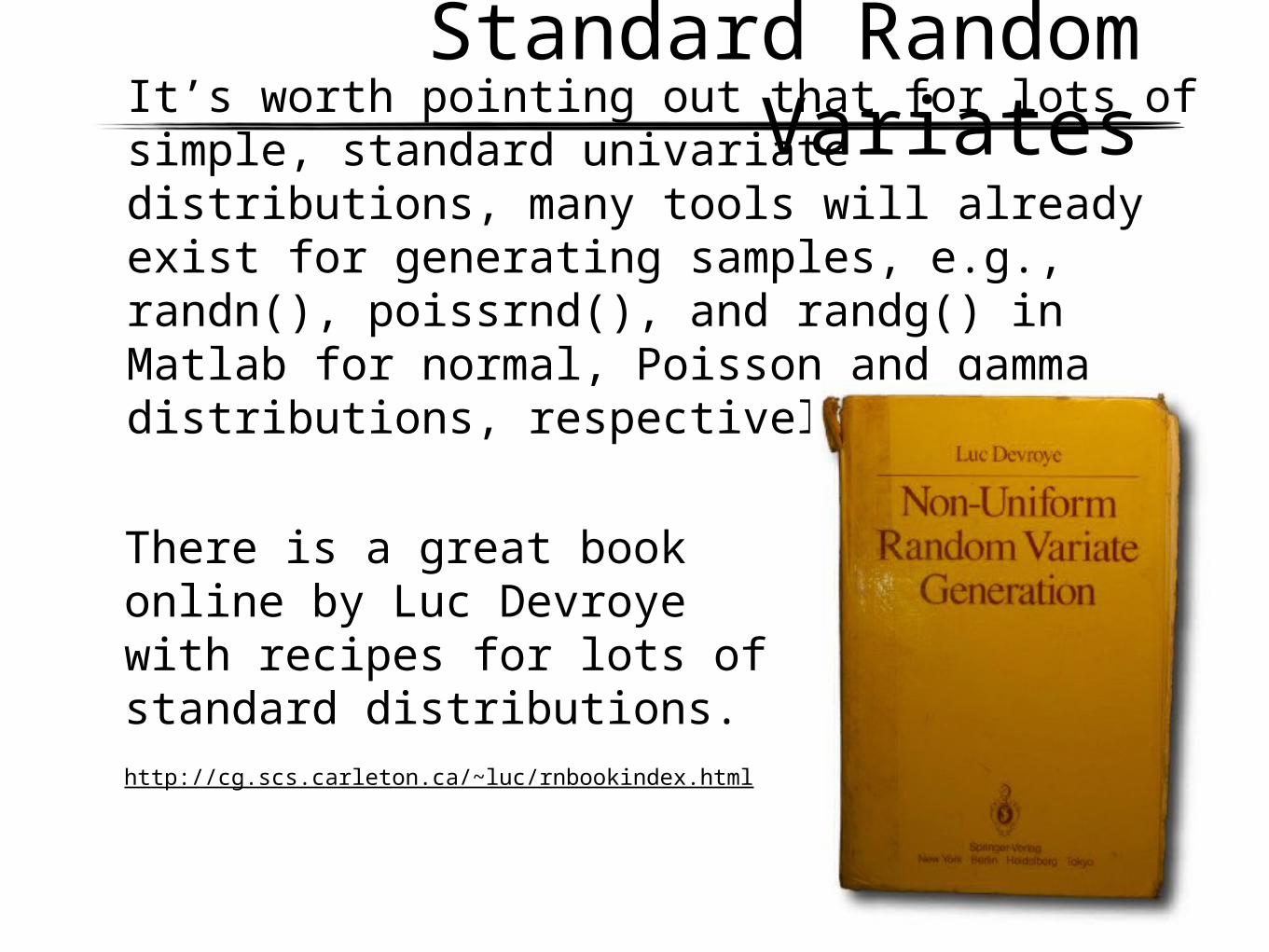
Standard Random VariatesIt’s worth pointing out that for lots of simple,

standard univariate distributions, many tools will already exist for generating samples, e.g., randn(), poissrnd(), and randg() in Matlab for normal, Poisson and gamma distributions, respectively.

There is a great book online by Luc Devroye with recipes for lots of standard distributions.http://cg.scs.carleton.ca/~luc/rnbookindex.html

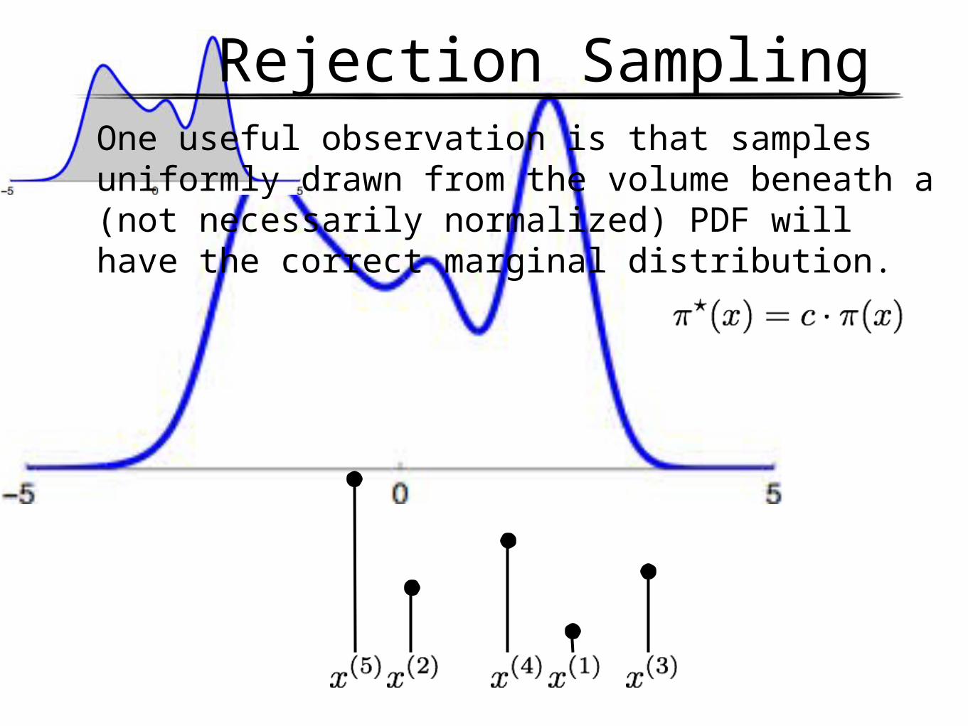
Rejection SamplingOne useful observation is that samples uniformly drawn from the volume beneath a (not necessarily normalized) PDF will have the correct marginal distribution.

Rejection SamplingHow to get samples from the area? This is the first example, of sample from a simple to get samples from a complicated .

Rejection Sampling

1. Choose and so that

2. Sample

3. Sample

4. If keep , else reject and goto 2.

If you accept, you get an unbiased sample from . Isn’t it wasteful to throw away all those proposals?

Importance Sampling

Recall that we’re really just after an expectation.

We could write the above integral another way:

Importance Sampling

We can now write a Monte Carlo estimate that is also an expectation under the “easy” distribution

We don’t get samples from , so no easy visualization of fantasy data, but we do get an unbiased estimator of whatever expectation we’re interested in.

It’s like we’re “correcting” each sample with a weight.

Importance Sampling

As a side note, this trick also works with integrals that do not correspond to expectations.

Scaling Up

Both rejection and importance sampling depend heavily on having a that is very similar to

In interesting high-dimensional problems, it is very hard to choose a that is “easy” and also resembles the fancy distribution you’re interested in.

The whole point is that you’re trying to use a powerful model to capture, say, the statistics of natural images in a way that isn’t captured by a simple distribution!

Exploding Importance WeightsEven without going into high dimensions, we

can see how a mismatch between the distributions can cause a few importance weights to grow very large.

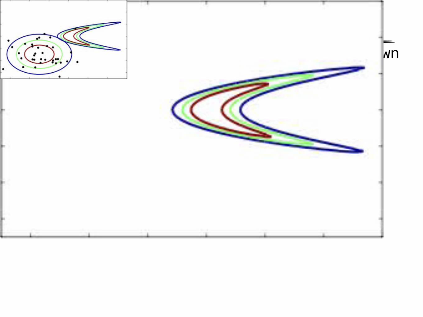
Scaling UpIn high dimensions, the mismatch between the proposal distribution and the true distribution can really ramp up quickly. Example:

Rejection sampling requires and accepts with probability . For the acceptance rate will be less than one percent.The variance of the importance sampling weights will grow exponentially with dimension. That means that in high dimensions, the answer will be dominated by only a few of the samples.

Summary So FarWe would like to find statistics of our probabilistic models for inference, learning and prediction.

Computation of these quantities often involves difficult integrals or sums.

Monte Carlo approximates these with sample averages.

Rejection sampling provides unbiased samples from a complex distribution.

Importance sampling provides an unbiased estimator of a difficult expectation by “correcting” another expectation.

Neither of these methods scale well in high dimensions.

Revisiting IndependenceIt’s hard to find the mass of an unknown density!

Revisiting IndependenceWhy should we immediately forget that we discovered a place with high density? Can we use that information?

Storing this information will mean that the sequence now has correlations in it. Does this matter?

Can we do this in a principled way so that we get good estimates of the expectations we’re interested in?

Markov chain Monte Carlo

Markov chain Monte Carlo

As in rejection and importance sampling, in MCMC we have some kind of “easy” distribution that we use to compute something about our “hard” distribution .

The difference is that we’re going to use the easy distribution to update our current state, rather than to draw a new one from scratch.

If the update depends only on the current state, then it is Markovian. Sequentially making these random updates will correspond to simulating a Markov chain.

Markov chain Monte Carlo

We define a Markov transition operator

The trick is: if we choose the transition operator carefully, the marginal distribution over the state at any given instant can have our distribution If the marginal distribution is correct, then our estimator for the expectation is unbiased.

Markov chain Monte Carlo

A Discrete Transition Operator

is an invariant distribution of , i.e.

is the equilibrium distribution of , i.e.

is ergodic, i.e., for all there exists a such that

Detailed BalanceIn practice, most MCMC transition operators satisfy detailed balance, which is stronger than invariance.

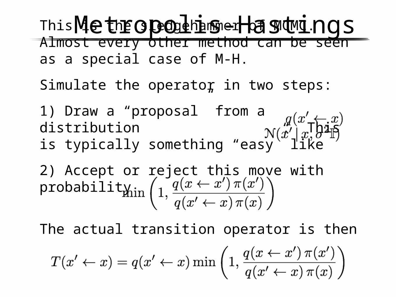
Metropolis-HastingsThis is the sledgehammer of MCMC. Almost every other method can be seen as a special case of M-H.

Simulate the operator in two steps:

1) Draw a “proposal” from a distribution . This is typically something “easy” like

2) Accept or reject this move with probability

The actual transition operator is then

Metropolis-HastingsThings to note:

1) If you reject, the new state is a copy of the current state. Unlike rejection sampling, the rejections count.

2) only needs to be known to a constant.

3) The proposal needs to allow ergodicity.

4) The operator satisfies detailed balance.

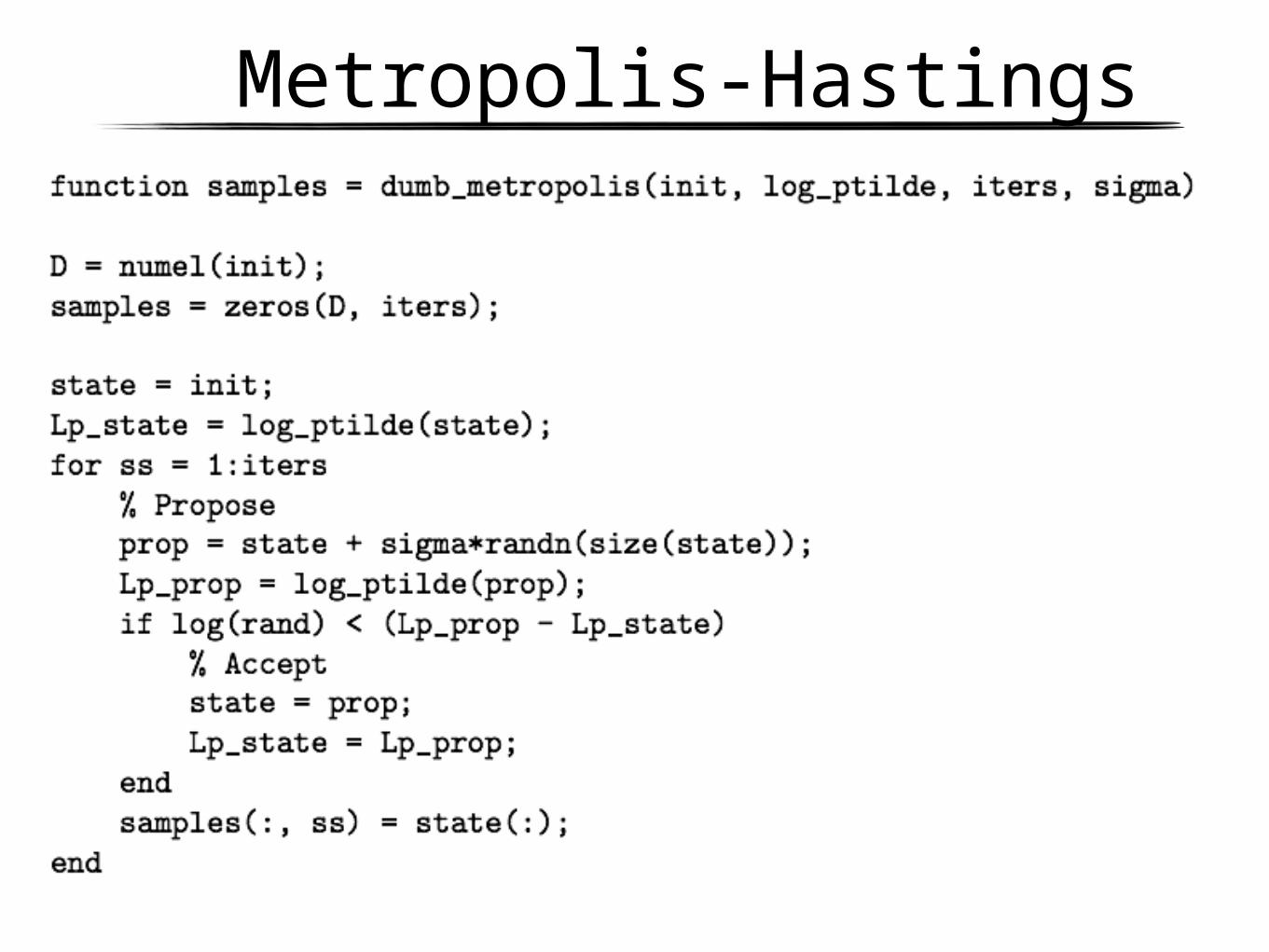
Metropolis-Hastings

Effect of M-H Step Size

Effect of M-H Step Size

Huge step size = lots of rejections

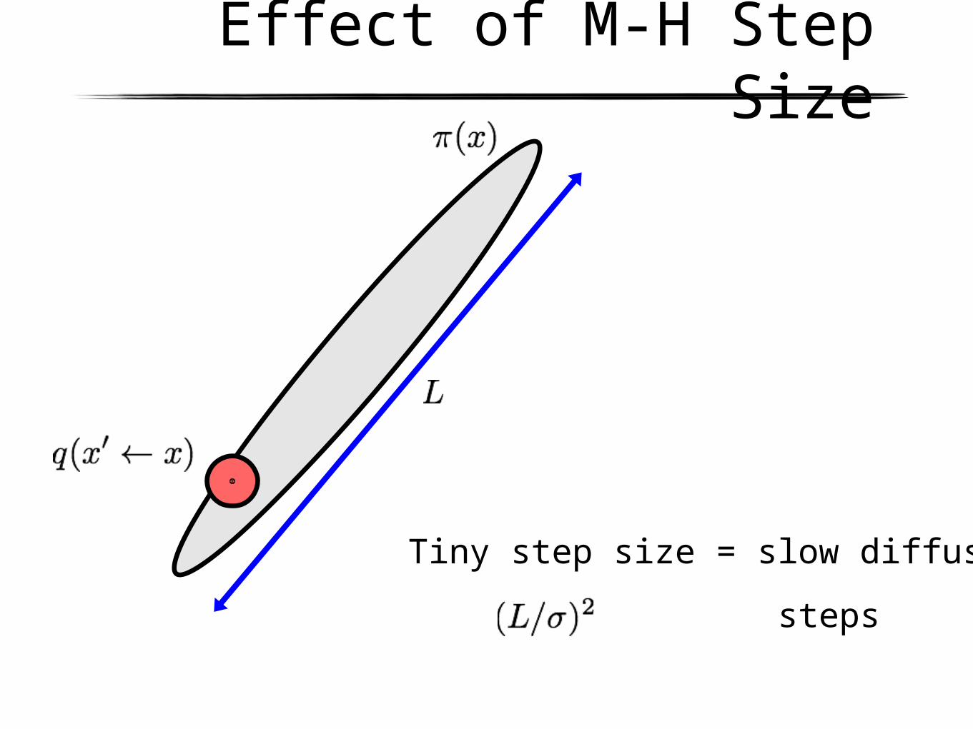
Effect of M-H Step Size

Tiny step size = slow diffusion

steps

Gibbs SamplingOne special case of Metropolis-Hastings is very popular and does not require any choice of step size.

Gibbs sampling is the composition of a sequence of M-H transition operators, each of which acts upon a single component of the state space.

By themselves, these operators are not ergodic, but in aggregate they typically are.

Most commonly, the proposal distribution is taken to be the conditional distribution, given the rest of the state. This causes the acceptance ratio to always be one and is often easy because it is low-dimensional.

Gibbs Sampling

Gibbs SamplingSometimes, it’s really easy: if there are only a small number of possible states, they can be enumerated and normalized easily, e.g. binary hidden units in a restricted Boltzmann machine.

When groups of variables are jointly sampled given everything else, it is called “block-Gibbs” sampling.

Parallelization of Gibbs updates is possible if the conditional independence structure allows it. RBMs are a good example of this also.

Summary So FarWe don’t have to start our sampler over every time!

We can use our “easy” distribution to get correlated samples from the “hard” distribution.

Even though correlated, they still have the correct marginal distribution, so we get the right estimator.

Designing an MCMC operator sounds harder than it is.

Metropolis-Hastings can require some tuning.

Gibbs sampling can be an easy version to implement.

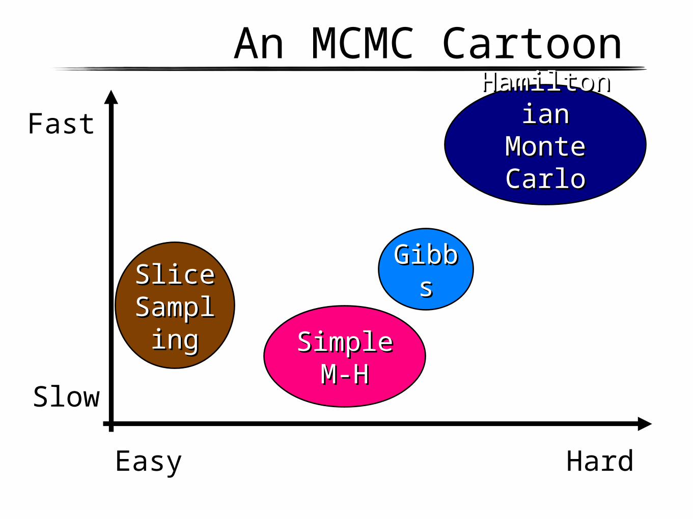
An MCMC Cartoon

Fast

Slow

Easy Hard

GibbGibbss

Simple Simple M-HM-H

Slice Slice SampSamplingling

HamiltoniHamiltonian Monte an Monte

CarloCarlo

Slice SamplingAn auxiliary variable MCMC method that requires almost no tuning. Remember back to the beginning...

Slice SamplingDefine a Markov chain that samples uniformly from the area beneath the curve. This means that we need to introduce a “height” into the MCMC sampler.

Slice SamplingThere are also fancier versions that will automatically grow the bracket if it is too small. Radford Neal’s paper discusses this and many other ideas.Radford M. Neal, “Slice Sampling”, Annals of Statistics 31, 705-767, 2003.Iain Murray has Matlab code on the web. I have Python code on the web also. The Matlab statistics toolbox includes a slicesample() function these days.

It is easy and requires almost no tuning. If you’re currently solving a problem with Metropolis-Hastings, you should give this a try. Remember, the “best” M-H step size may vary, even with a single run!

Multiple DimensionsOne Approach: Slice sample each dimension, as in Gibbs

Multiple DimensionsAnother Approach: Slice sample in random directions

Auxiliary VariablesSlice sampling is an example of a very useful trick.

Getting marginal distributions in MCMC is easy: just throw away the things you’re not interested in.

Sometimes it is easy to create an expanded joint distribution that is easier to sample from, but has the marginal distribution that you’re interested in.

In slice sampling, this is the height variable.

An MCMC Cartoon

Fast

Slow

Easy Hard

GibbGibbss

Simple Simple M-HM-H

Slice Slice SampSamplingling

HamiltoniHamiltonian Monte an Monte

CarloCarlo

Avoiding Random WalksAll of the MCMC methods I’ve talked about so far have been based on biased random walks.

You need to go about to get a new sample, but you can only take steps around size , so you have to expect it to take about

Hamiltonian Monte Carlo is about turning this into

Hamiltonian Monte CarloHamiltonian (also “hybrid”) Monte Carlo does MCMC by sampling from a fictitious dynamical system. It suppresses random walk behaviour via persistent motion.

Think of it as rolling a ball along a surface in such a way that the Markov chain has all of the properties we want.

Call the negative log probability an “energy”.

Think of this as a “gravitational potential energy” for the rolling ball. The ball wants to roll downhill towards low energy (high probability) regions.

Hamiltonian Monte CarloNow, introduce auxiliary variables (with the same dimensionality as our state space) that we will call “momenta”.

Give these momenta a distribution and call the negative log probability of that the “kinetic energy”. A convenient form is (not surprisingly) the unit-variance Gaussian.

As with other auxiliary variable methods, marginalizing out the momenta gives us back the distribution of interest.

Hamiltonian Monte CarloWe can now simulate Hamiltonian dynamics, i.e., roll the ball around the surface. Even as the energy sloshes between potential and kinetic, the Hamiltonian is constant.

The corresponding joint distribution is invariant to this.This is not ergodic, of course. This is usually resolved by randomizing the momenta, which is easy because they are independent and Gaussian.

So, HMC consists of two kind of MCMC moves:

1) Randomize the momenta.

2) Simulate the dynamics, starting with these momenta.

Alternating HMC

Perturbative HMC

HMC Leapfrog IntegrationOn a real computer, you can’t actually simulate

the true Hamiltonian dynamics, because you have to discretize.

To have a valid MCMC algorithm, the simulator needs to be reversible and satisfy the other requirements.

The easiest way to do this is with the “leapfrog method”:

The Hamiltonian is not conserved, so you accept/reject via Metropolis-Hastings on the overall joint distribution.

Overall SummaryMonte Carlo allows you to estimate integrals that may be impossible for deterministic numerical methods.

Sampling from arbitrary distributions can be done pretty easily in low dimensions.

MCMC allows us to generate samples in high dimensions.

Metropolis-Hastings and Gibbs sampling are popular, but you should probably consider slice sampling instead.

If you have a difficult high-dimensional problem, Hamiltonian Monte Carlo may be for you.