MONTE CARLO LOCALIZATION FOR MOBILE ROBOTS A THESIS …
77
MONTE CARLO LOCALIZATION FOR MOBILE ROBOTS IN DYNAMIC ENVIRONMENTS by AJAY BANSAL, B.Tech. A THESIS IN COMPUTER SCIENCE Submitted to the Graduate Faculty of Texas Tech University in Partial Fulfillment of the Requirements for the Degree of MASTER OF SCIENCE Approved May, 2002
Transcript of MONTE CARLO LOCALIZATION FOR MOBILE ROBOTS A THESIS …

MONTE CARLO LOCALIZATION FOR MOBILE ROBOTS
IN DYNAMIC ENVIRONMENTS
by
AJAY BANSAL, B.Tech.
A THESIS
IN
COMPUTER SCIENCE
Submitted to the Graduate Faculty
of Texas Tech University in Partial Fulfillment of the Requirements for
the Degree of
MASTER OF SCIENCE
Approved
May, 2002

ACKNOWLEDGEMENTS
At the very outset, I would like to extend my heartfelt gratitude to my research
advisor. Dr. Lairy Pyeatt. His constant guidance and tireless monitoring of my work
inspired me to deliver my best effort. I am deeply thankful to Dr. W. B. J. Oldham and
Dr. Richard Watson for so kindly having consented to being on my thesis committee.
Their insights and points of view were cornerstones to my path of reasoning and
methodology.
And last, but not least, I would like to express my gratitude and thanks to the
Department of Computer Science, Texas Tech University, for having provided me the
excellent infrastructure for conducting my research work.

TABLE OF CONTENTS
ACKNOWLEDGEMENTS ii
ABSTRACT v
LIST OF FIGURES vi
CHAPTER
1. INTRODUCTION 1
1.1 Objectives 1
1.2 Document Organization 5
2. MONTE CARLO LOCALIZATION 6
2.1 Bayes Filtering 6
2.2 Probabilistic Models for Localization 9
2.3 Particle Approximation 11
2.4 The MCL Algorithm 13
2.5 Limitations of MCL 14
3. FILTERING TECHNIQUES 15
3.1 Filtering Techniques for Dynamic Environments 15
3.2 Entropy Filter 16
3.3 Distance Filter 17
3.4 The MCL Algorithm with Filtering Techniques. 19

4. EXPERIMENTAL SETUP 21
4.1 Experimental Robot 21
4.2 fhe Graphical Interface 21
4.3 Programming the Robot 29
4.4 The Global Vectors 33
4.5 Robot Commands 35
4.5.1 Communication Commands 36
4.5.2 Motion Commands 36
4.5.3 Sensing Commands 37
4.5.4 Server Commands 37
5. IMPLEMENTATION 38
6. COMPARISON AND ANALYSIS 45
7. CONCLUSIONS AND FUTURE WORK 50
REFERENCES 51
APPENDED 53

ABSTRACT
Mobile robot localization is the problem of determining a robot's pose from
sensor data. This thesis presents a family of probabilistic localization algorithms known
as Monte Carlo Localization (MCL). MCL algorithms represent a robot's belief by a set
of weighted hypotheses (samples) which approximate the posterior under a common
Bayesian formulation of the localization problem. The MCL algorithm does not work
well in dynamic environments. Thus, building on the basic MCL algorithm, this thesis
develops a dynamic version of the algorithm, which applies filtering techniques to filter
out the unexpected data and work well in dynamic environments. Systematic empirical
results illustrate the robustness and computational efficiency of the approach.

LIST OF FIGURES
: . l The MCL Algorithm 13
3.1 The MCL Algorithm with Filtering Techniques 20
4.1 The Graphical Interface 22
4.2 The Four Main Windows of the Robot Simulator 23
4.3 The Map Window 25
4.4 The Robot Window 26
4.5 Place Robot 27
4.6 The ShortSensor Window 28
4.7 The LongSensorWindow 29
4.8 Programming in Direct and Client Mode 30
4.9 Sample program to mn the robot 32
4.10 The arrangement of the Bumper Sensors 34
5.1 Input Map 1 38
5.2 Input Map 2 39
5.3 Skeleton of MCL Algonthm 40
6.1 Input Mapl with 5 unknown obstacles 45
6.2 Input Map 2 with 3 unknown obstacles 46
6.3 Performance of MCL with Filters 47
6.4 Input Map 2 with a large number of unknown obstacles 48
6.5 Input Map 1 with unknown obstacles all around the robot 49

CHAPTER 1
INTRODUCTION
1.1 Objectives
Robot localization has been recognized as one of the most fiindamental problems
in mobile robotics [14]. The aim of localization is to estimate the position of a robot in its
environment, given a map of the environment and sensor data. Most successful mobile
robot systems to date utilize some type of localization, as knowledge of the robot's
position is essential for a broad range of mobile robot tasks.
Localization often referred to as position estimation or position control [13] is
currently a highly active field of research. The localization techniques developed so far
can be distinguished according to the type of problem they attack. Tracking or local
techniques aim at compensating odometric errors occurring during robot navigation.
They require, however, that the initial location of the robot be (approximately) known,
and they typically cannot recover if they lose track of the robot's position (within certain
bounds). Another family of approaches is called global techniques. These are designed to
estimate the position of the robot even under global uncertainty. Techniques of this type
solve the so-called wake-up robot problem, in that they can localize a robot without any
prior knowledge about its position. They fiirthermore can handle the kidnapped robot
problem, in which a robot is carried to an arbitrary location during its operation. Global
localization techniques are more powerful than local ones. They typically can cope with
situations in which the robot is likely to experience serious positioning enors. Finally, all

these problems are particulariy difficult in dynamic environments, e.g., if robots operate
in the proximity of people who corrupt the robot's sensor measurements.
The vast majority of existing algorithms address only the position tracking. The
nature of small, incremental errors makes algorithms such as Kalman filters [22]
applicable, which have been successfully applied in a range of fielded systems. Kalman
filters estimate posterior distributions of robot poses conditioned on sensor data.
Exploiting a range of restrictive assumptions—such as Gaussian-distributed noise and
Gaussian-distributed initial uncertainty, they represent posteriors by Gaussians,
exploiting an elegant and highly efficient algorithm for incorporating new sensor data.
However, the restrictive nature of the belief representations makes them unapplicable to
global localization problems in which a single Gaussian does not accurately reflect the
tme distribution.
This limitation is overcome by two related families of algorithms: localization
with multi-hypothesis Kalman filters and Markov localization [2]. Multi-hypothesis
Kalman filters represent beliefs using mixtures of Gaussians, thereby enabling them to
pursue multiple, distinct hypotheses, each of which is represented by a separate Gaussian.
However, this approach inherits from Kalman filters the Gaussian noise assumption. To
meet this assumption, virtually all practical implementations extract low-dimensional
features from the sensor data, thereby ignoring much of the information acquired by a
robot's sensors. Markov localization algorithms, in contrast, represent beliefs by
piecewise constant functions (histograms) over the space of all possible poses. Just like
Gaussian mixtures, piecewise constant fiinctions are capable of complex, multi-modal
representations. However, accommodating raw sensor data requires fine-grained
representations, which impose significant computational burdens. To overcome this
limitation, researchers have proposed selective updating algorithms and tree-based
representations that dynamically change their resolution. It is remarkable that all of these
algorithms share the same probabilistic basis.
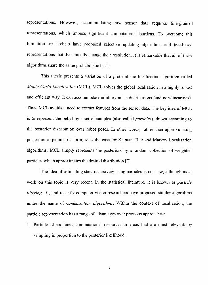
This thesis presents a variation of a probabilistic localization algorithm called
Monte Carlo Localization (MCL). MCL solves the global localization in a highly robust
and efficient way. ft can accommodate arbitrary noise distributions (and non-linearities).
Thus, MCL avoids a need to extract features from the sensor data. The key idea of MCL
is to represent the belief by a set of samples (also called particles), drawn according to
the posterior distribution over robot poses. In other words, rather than approximating
posteriors in parametric form, as is the case for Kalman filter and Markov Localization
algorithms, MCL simply represents the posteriors by a random collection of weighted
particles which approximates the desired distribution [7].
The idea of estimating state recursively using particles is not new, although most
work on this topic is very recent. In the statistical literature, it is known as particle
filtering [5], and recently computer vision researchers have proposed similar algorithms
under the name of condensation algorithms. Within the context of localization, the
particle representation has a range of advantages over previous approaches:
1. Particle filters focus computational resources in areas that are most relevant, by
sampling in proportion to the posterior likelihood.

2. Particle filters are universal density approximators, weakening the restrictive
assumptions on the shape of the posterior density when compared to previous
parametric approaches.
3. Particle filters are easily implemented as any-time algorithms, which are algorithms
that can output an answer at any time, but where the quality of the answer depends on
the time spent computing it. By controlling the number of samples on-line, particle
filters can adapt to the available computational resources. The same code can, thus, be
executed on computers with vastly different speed without modification of the basic
code.
4. Finally, particle filters are surprisingly easy to implement, which makes them an
attractive paradigm for mobile robot localization. Consequentiy, it has already been
adopted by several research teams, who have extended the basic paradigm in
interesting new ways [1].
However, there are pitfalls, too, arising from the stochastic nature of the
approximation. Some of these pitfalls are obvious: for example, if the sample set size is
small, a well-localized robot might lose track of its position just because MCL fails to
generate a sample in the right location. The MCL algorithm is also unfit for the
kidnapped robot problem, since there might be no surviving samples near the robot's new
pose after it has been kidnapped. Somewhat counter-intuitive is the fact that the basic
algorithm degrades when sensors are too accurate. In extreme, MCL will fail with
perfect, noise free sensors. Most importantly, however, the MCL algorithm assumes that
the environment is static. Therefore, they typically fail in highly dynamic environments.
such as public places where crowds of people may cover the robot's sensors for extended
periods of time.
This thesis presents a version of MCL which uses filtering techniques with the
basic algorithm to make it work in highly dynamic environments. The key idea is to filter
out the unexpected sensor data, coming from unknown objects and update the position
belief of the robot using only those measurements which are with high likelihood
produced by known objects contained in the map. As a result it permits accurate
localization even in densely crowded, non-static environments [2].
1.2 Document Organization
The first chapter on Introduction discussed the outline of the thesis problem and
the motivation for this research work. Chapter 2 deals with the basic concepts involved in
the Monte Carlo Localization algorithm and its limitations. The proposed solution, the
filtering techniques that enable the Monte Carlo Localization algorithm to work in
dynamic environments is discussed in detail in Chapter 3. Chapter 4 describes the
experimental setup. Implementation is described in Chapter 5. Comparison of this
implementation with the existing algorithms is presented in Chapter 6. Chapter 7
concludes the thesis with statements of results obtained and future work.
CHAPTER 2
MONTE CARLO LOCALIZATION
2.1 Bayes Filtering
MCL is a recursive Bayes filter that estimates the posterior distribution of robot
poses conditioned on sensor data. Bayes filters address the problem of estimating the
state .V of a dynamical system (partially observable Markov chain) from sensor
measurements. For example, in mobile robot localization the dynamical system is a
mobile robot and its environment, the state is the robot's pose therein (often specified by
a position in a two-dimensional Cartesian space and the robot's heading direction G), and
measurements may include range measurements, camera images, and odometry readings.
Bayes filters assume that the environment is ''Markovian" (static) [2], that is, past and
future data are (conditionally) independent if one knows the current state. The Markov
assumption is made more explicit below.
The key idea of Bayes filtering is to estimate a probability density over the state
space conditioned on the data. This posterior is typically called the belief and is denoted
by
Bel{x,)^ p{x, |fi?o.. ,)•
Here x denotes the state, x, is the state at time t, and d^ , denotes the data starting at time
0 up to time t. For mobile robots, we distinguish two types of data: perceptual data such
as laser range measurements, and odometry data, which carry information about robot

motion. Denoting the former by o (for observation) and the latter by a (for action), we
have
Bel{x,)^ p(x, |o,,a,_,,o,_|,a,_2,...,oJ. (2.1)
Without loss of generality, we assume that observations and actions arrive in an
alternating sequence. Notice that we will use a,,, to refer to the odometry reading that
measures the motion that occurred in the time interval [/-/; /], to illustrate that the motion
is the result of the control action asserted at time t-1.
Bayes filters estimate the belief recursively. The initial belief characterizes the
initial knowledge about the system state. In the absence of such knowledge, it is typically
initialized by a uniform distribution over the state space. In mobile robot localization, a
uniform initial distribution corresponds to the global localization problem, where the
initial robot pose is unknown.
To derive a recursive update equation, we observe that equation (2.1) can be
transformed by Bayes mle to
Bel{x,) = rip{o, \x,,a,_^,o,_„a,_^,...,oJp{x, \a,_„o,_^,a,_^,...,o^) (2.2)
where r) is a is a normalization constant. As noticed above, Bayes filters rest on the
assumption that fuUire data is independent of past data given knowledge of the current
state—an assumption typically referred to as the Markov assumption [2]. Put
mathematically, the Markov assumption implies
/)(o, lx,,fl,_,,o,.,,a,_2,...,oJ = p(o, \x,) (2.3)
and hence our target equation (2.2) can be simplified to
Bel{x,)^r]p{o, \x,)p{x, \ a,_,,o,_^,a,^^,...,o„). (2.4)
We will now expand the rightmost term by integrating over the state at time t-1:
Bel{xJ = r]p{o, |.v,)lp(..v, \ x, _^,a,_,,...,oJp{x,_, \a,^,,o,_^,a,_^,...,oJdx,_^. (2.5)
Again we exploit the Markov assumption to simplify p(x, | x,_^,a,_^,...,Of^):
P{\ |v,.,,fl,_,,...,Oo) = /'(- ', l- ', i>«,-i) (2.6)
which gives us the expression:
Bel{x,) = r]p{o, |x,)jp(x, \x,_,,a,_^)p{x,_^ \a,_„o,_„a,_^,...,o^)dx,_^. (2.7)
Substituting the basic definition of the belief 5e/ back into (2.7), we obtain the important
recursive equation
Bel{x,) = r]p{o, \x,)\p{x, \ x,.,,a,., )Bel{x,_^ )dx,_^. (2.8)
This equation is the recursive update equation in Bayesian filters. Together with the
initial belief, it defines a recursive estimator for the state of a partially observable system.
This equation is of central importance, as it is the basis for various MCL algorithms.
To implement (2.8), one needs to know two conditional densities: the probability
p{x, I X|_^,a|_^), which we will refer to as next state density or simply Motion Model, and
the density p(o, | x,) , which we will call Perceptual Model or Sensor Model. If the
Markov assumption holds, then both models are typically stationary (also called: time-
invariant), that is, they do not depend on the specific time t. This stationarity allows us to
simplify the notation by denoting these models p (x\x', a), and p(o \ x), respectively.

2.2 Probabilistic Models for Localization
The naUire of the models p (x | x'. a), and p (o \ x), depends on the specific
estimation problem. In mobile robot localization, both models are relatively
straightforward and can be iinplemented in a few lines of code.
The motion model, p(x \ x', a), is a probabilistic generalization of robot
kinematics. More specifically .v and x' are poses. For a robot operating in the plane, a
pose IS a three-dimensional variable that comprises of a robot's two-dimensional
Cartesian co-ordinates and its heading direction (orientation). The value of a may be an
odometry reading or a control command, both of which characterize the change of pose.
In robotics, equations describing change of pose due to controlled and uncontrolled
variables are called kinematics. The conventional kinematic equations, however, describe
only the expected pose x that an ideal, noise-free robot would attain starting at x', and
after moving as specified by a. Of course, physical robot motion is probabilistic due to
many reasons like slippage of wheels and motors, imprecise measurements and other
sources of uncertainty; thus, the pose x is uncertain. To account for this inherent
uncertainty, the probabilistic motion modelpfx \x' ,a), describes a posterior density over
possible successors x. Noise is typically modeled by zero centered, Gaussian noise that is
added to the translation and rotation components in the odometry measurements. Thus,
p(x I x', a), generalizes exact mobile robot kinematics.
For the MCL algorithm described further below, one does not need a closed-form
description of the motion model/?(x | x', a). Instead, a sampling model [1] ofp(x \ x', a)
suffices. A sampling model is a routine that accepts x' and a as input and generates

random poses .Y distributed according to p(x | .v', a). Sampling models are usually easier
to code than routines that compute densities in closed form.
Let us now turn our attention to the perceptual model, p(o \ x). Mobile robots are
commonly equipped with range finders, such as ultrasonic transducers (sonar sensors) or
laser range finders. For range finders, we decompose the problem of computing p (o \ x)
into three parts:
1. the computation of the value a noise-free sensor would generate;
2. the modeling of sensor noise; and
3. the integration of many individual sensor beams into a single density value.
Assume the robot's pose is x, and let o, denote an individual sensor beam with bearing
a, relative to the robot. Let g (x, a.) denote the measurement of an ideal, noise-free
sensor whose relative bearing is a , . Since we assume that the robot is given a map of the
environment, g (x a.) can be computed using ray tracing. It is a common practice to
assume that this "expected" distance g (x, a,, j is a sufficient statistic for the probability/?
(o, I x), that is
p(o. \x)= p(o. I g(x, a,. j j . (2.9)
The exact density p (o ^ \ x) is a mixture of three densities: a Gaussian centered at
g (x, a.) that models the event of measuring the correct distance with small added
Gaussian noise, an exponential density that models random readings as often caused by
people, and a discrete large probability (mathematically modeled by a narrow uniform
10

density) that models max-range measurements, which frequently occur when a range
sensor fails to detect an object.
Finally, the individual density values;? (a. \ x) are integrated multiplicatively,
assuming conditional independence between the individual measurements:
P(o\x)=Y\,p{o,\x). (2.10)
Clearly, this conditional independence can be violated in the presence of people (which
often block more than one sensor beam), that is when the environment is non-Markovian
or dynamic.
2.3 Particle Approximation
If the state space is continuous, as is the case in mobile robot localization,
implementing (2.8) is not a trivial matter—particularly if one is concemed about
efficiency. The idea of MCL (and other particle filter algorithms) is to represent the belief
Bel(x) by a set of m weighted samples distributed according to Bel(x):
Here each .\"'is a sample (a hypothesized state), and w'" are non-negative numerical
factors called importance factors, which are assumed to sum to one. As the name
suggests, the importance factors determine the weight (importance) of each sample [7].
The initial set of samples represents the initial knowledge Bel(xJ about the state
of the dynamical system. In global mobile robot localization, the initial belief is a set of
11

poses drawn according to a uniform distribution over the robot's universe, annotated by
the uniform importance factor 1/m.
The recursive update is realized in three steps.
1. Sample .v"',-i * iSe/(A-,_|)from the (weighted) sample set representing Bel(x,_^).
Each such particle .v"',-i is distributed according to the belief distribution Bel{x,_^).
2. Sample -v'", « p(.v, | .v<",-i,a,_,). Obviously, the pan <x*'\,x"',-i >is distributed
according to the product distribution
9, •=p{x, \x,_„a,_,)*Bel{x,_,) (2.11)
which is commonly called the proposal distribution.
3. To offset the difference between the proposal distribution and the desired distribution
specified in Equation (2.8)
Wio, \x,)p{x, |x,_|,fl,_,)5e/(x,_,) (2.12)
the sample is weighted by the quotient
,,, _ T]p{o, |X"',)/?(A-"', |x'"",-i,fl,_,)^e/(x"Vi) "W? — ——-
5e/(x"^-,);?(x"*, |x"-",-,,a,_,)
ocp(o, |x<",) (2.13)
w*" denotes the new (non-normalized) importance factor for the particle x^'\ .
The sampling routine is repeated m times, producing a set of m weighted samples \^'\.
Afterwards, the importance factors are normalized so that they sum to one and hence
define a discrete probability distribution.
12

2.4 The MCL Algorithm
Figure 2.1 summarizes the MCL algorithm. It is known [23] that under mild
assumptions, the sample set converges to the tme posterior 5e/(x,) as m goes to infinity,
with a convergence speed in 0{—r=). The speed may vary by a constant factor, which
can \ ary drastically depending on the proposal distribution. Due to the normalization, the
particle filter is only asymptotically unbiased. The bias increases as the sample set size
decreases. If the number of samples is large, then the bias can be neglected.
Algorithm MCL(X, a, o):
T = (i>
for I = 0 to m do
Generate random x
Generate random x
W' = p(o 1 x' ,m)
Add <x', w'>toX"
Endfor
Normalize the importance
retumZ'
from X according
' -P(x
factors
1 a, x)
wmX"
to w,,...,w„
Figure 2.1. The MCL Algorithm
13

2.5 Limitations of MCL
Some of the limitations of the MCL algorithm are obvious. The basic particle
filter performs poorly if the proposal distribution, which is used to generate samples,
places too little samples in regions where the desired posterior Bel{x,) is large. Also, if
the sample set size is small, a well-localized robot might lose track of its position Just
because MCL fails to generate a sample in the right location. The MCL algorithm is also
unfit for the kidnapped robot problem, since there might be no surviving samples nearby
the robot's new pose after it has been kidnapped. In extreme, MCL will fail with perfect,
noise free sensors. In other words, MCL with accurate sensors may perform worse than
MCL with inaccurate sensors. This finding is a bit counter-intuitive in that it suggests that
MCL only works well in specific situations, namely those where the sensors possess the
"right" amount of noise. Most importantly, however, the MCL algorithm assumes that the
environment is static. Therefore, they typically fail in highly dynamic environments, such
as public places where crowds of people may cover the robot's sensors for extended
periods of time. This thesis proposes to solve the above mentioned most important
problem with MCL (the static worid assumption, when actually the worid is not static).
The next chapter describes in detail the proposed solution.
14

CHAPTER 3
FILTERING TECHNIQUES
3.1 Filtering Techniques for Dynamic Environments
Monte Carlo Localization has been shown to be robust to occasional changes of
an environment such as opened/closed doors or people walking by. Unfortunately, it fails
to localize a robot if too many aspects of the environment are not covered by the world
model. This is the case, for example, in densely crowded environments, where groups of
people cover the robot's sensors and thus lead to many unexpected measurements.
The reason why Monte Carlo Localization fails in such situations is the violation
of the Markov assumption, an independence assumption on which virtually all
localization techniques are based. This assumption states that the sensor measurements
observed at time t are independent of all other measurements, given that the cunent state
of the world is known. In the case of localization in densely populated environments, this
independence assumption is clearly violated when using a static model of the world.
A closely related solution to this problem could be to adapt the map according to
the changes of the environment. Techniques for concunent map building and
localization, however, also assume that the environment is almost static and therefore are
unable to deal with such environments. Another approach would be to adapt the
perception model to correctiy reflect such situations. Unfortunately, such approaches are
only able to model such noise on average. While such approaches work reliably with
occasional sensor blockage, they are not sufficient in situations where more than fifty
15

percent of the sensor measurements are corrupted [2]. The localization system in this
thesis includes filters that are designed to detect whether a certain sensor reading is
corrupted or not. Compared to a modification of the static sensor model described above,
these filters have the advantage that they do not average over all possible situations and
that their decision is based on the current belief of the robot. The filters are designed to
select those readings of a complete scan which do not come from objects contained in the
map. As a result, it permits accurate localization even in densely crowded, non-static
environments. In this section two different kinds of filters are introduced. The first one is
called an Entropy Filter. Since it filters a reading based solely on its effect on the belief
Bel(x), it can be applied to arbitrary sensors. The second filter is the distance filter that
selects the readings according to how much shorter they are than the expected value. It
therefore is especially designed for proximity sensors [2].
3.2 Entropy Filter
The entropy H(X) of the belief over X is defined as
H(X) = E, Bel(X =x) log Bel(X =x)
and is a measure of uncertainty about the outcome of the random variable X. The higher
the entropy, the higher the robot's uncertainty as to where it is. The entropy filter
measures the relative change of entropy upon incorporating a sensor reading into the
belief 5e/ (X). More specifically, let o denote the measurement of a sensor. The change of
the entropy of Bel(X) given o is defined as:
AH(X\o):=H(X\o) H(X) .
16

The temi H(X \ o) is the entropy of the heWef Bel(X) after incorporating the sensor
measurement o. While a positive change of entropy indicates that after incorporating o,
the robot is less certain about its position, a negative change indicates an increase in
certainty. The selection scheme of the entropy filter is to exclude all sensor measurements
o with A H(X I o) < 0. In other words, it only uses those sensor readings confirming the
robot's current belief
Entropy filters work well when the robot's belief is focused on the correct
hypothesis. However, they may fail in situations in which the robot's belief state is
incorrect. The advantage of the entropy filter is that it makes no assumptions about the
nature of the sensor data and the kind of disturbances occurring in dynamic environments
[2].
3.3 Distance Filter
The distance filter is particularly useful for proximity sensors such as laser range
finders. Distance filters are based on a simple observation: In proximity sensing,
unmodeled obstacles typically produce readings that are shorter than the distance
expected from the map. In essence, the distance filter selects sensor readings based on
their distance relative to the distance to the closest obstacle in the map.
To be more specific, this filter removes those sensor measurements o which with
probability higher than y are shorter than expected, and which therefore are caused by an
unmodeled object (e.g., a person).
17

To see, let J,,..., </„ be a discrete set of possible distances measured by a
proximity sensor. Let P ,„(d^ \ x) be the probability of measuring distance d. if the robot
is at position .v and the sensor detects the closest obstacle in the map along the sensing
direction. The distribution P,„ describes the sensor measurement expected from the map.
This distribution is assumed to be Gaussian with mean at the distance o, to the closest
obstacle along the sensing direction.
1 - , _ 2
Now the probability P.^oni'^11 ^) that a measured distance rf,.is shorter than the
expected one given the robot is at position x can be defined. This probability is equivalent
to the probability that the expected measurement o, is longer than d. given the robot is at
location .v and thus can be computed as follows:
Ps.oM^x)-Y.PMM)•
hi practice, however, we are interested in the probability P,hcri(di) that J,.is
shorter than expected, given the complete current belief of the robot. Thus, we have to
average over all possible positions of the robot:
Ps.oAd.)-i:Ps.oAdAx)Bel{X = x). X
Given the distribution P ;,„,, (d.), we now can implement the distance filter by excluding
all sensor measurements c/,with P,„,JdJ > y, whereas the entropy filter fibers

measurements according to their effect on the belief state of the robot the distance filter
selects measurements solely based on their value and regardless of their effect on the
robot's certainty.
3.4 The MCL Algorithm with Filtering Techniques
The algorithm in Figure 3.1 filters out all the unwanted readings from the
en\ironment using the two mentioned filtering techniques and thus makes the MCL
algorithm work well in real time. The thesis work will consist of implementing this
algorithm (MCL with filtering technique) and evaluating its performance on a real
localization task.
19

Algorithm MCL(A', a, o):
If ((PassEntropyFilter(o) = FALSE) OR (PassDistanceFilter(o) =
Then RETURN.
X = (^
for i = 0 to m do
Generate random x from A'according to w,,..., w^
Generate randomx' vp (x' \ a, x)
u'' = p(o 1 A-', m)
add <x', w •> to X
endfor
normalize the importance factors winX
return A
-- FALSE))
Figure 3.1. The MCL Algorithm with Filtering Techniques
20

CHAPTER 4
EXPERIMENTAL SETUP
4.1 Experimental Robot
The research was performed on the simulator for the Super Scout, an integrated
mobile robot system with ultrasonic, tactile and odometry sensing. It uses a special
multiprocessor low-level control system that controls the sensing, motion, and
communications. At a high level, the Scout is controlled via an on-board PC computer.
Communication with the low-level is achieved through a server. The Server is a
convenient way to send commands to the robot and to receive sensing data from the
robot. It provides an elaborate graphic interface and simulation capabilities. The server is
mn as a separate process on a workstation. The server process communicates with the
robot process through ethemet, using the TCP/IP protocol. The server is by default
configured in simulation, which means that actions do not have physical consequences.
4.2 The Graphic Interface
The Graphic User Interface (GUI) provides a convenient access to the real and
simulated robots, and to the representation of the world, as shown in Figure 4.1. Through
the GUI, the user can send commands to the robot, monitor command execution by
seeing the robot actually moving on the screen and visualize instantaneous and cumulated
21

sensor data. The user can also create and modify a simulated environment, and use it to
test robot programs (Figure 4.2).
Client Pros ram
World Representation
it Graphical Interface
Server
Simulator
Figure 4.1 The Graphical Interface
22

023 Hie Edit Obslactos Vlow Sliow Control
Uindou bounds: LL(-00001620,-«(iij01840), IJ!<-.0O0W6M,t0OCOia48) Units: cccnjinates = 0.1 inches', angles = 0,1 decrees
•J^JIJ Robot View Show Relresh Panels
Window b o i ^ s : LL(-'X'O017C'O.-IXB;")2O3(I>, Uft<-»(''>X'i7O0,'0C"X'2' ftctual posit ion: K=*IX*OOCM:'0 Y=*«*0(X>00 S:rOijOO T=0000 Er»co.Jer posUlon; X=*C«>XiuOOi> Y='-iXXji)fiOO0 S=0000 T-OOOO Cofl¥>«s value: OOOO Previous co<wsnrf: norte yet Lhi ts; coordinates = 0.1 inches: angles = 0,1 deuces
ojiUons
'2y^
' " / / /
- . - i ^
/ . / /
\ \ ^ \
Figure 4.2 The Four Main Windows of Robot Simulator
23

The GUI presents 2 different views of the world. The different windows are
• The Map window
• One Robot window
• The Short Sensors and Long Sensors windows.
There is only one Map window, but as many Robot windows as there are robots(real
or simulated). The Map window gives access to the worid representation, with functions
such as: creating obstacles, editing obstacles, etc. The Robot window allows the display
of sensor history, the path of the robot, as well as the execution of robot commands. Both
windows support usual display functionalities like zooming and unzooming, scrolling,
centering, etc. Several display parameters are controlled by values set up in the file
world.setup.
4.2.1 The Simulator
There is no difference in the graphic display whether the interface is dealing with
a real or a simulated robot. By default, the GUI is in simulation mode. The REAL
ROBOT option of the ROBOT item in the Robot window is used to toggle between the
real and the simulated robot.
4.2.2 The Map Window
The Map window allows an application to interactively define and modify the
map of the world where a robot moves around. The robot world is an abstract coordinate
system; its dimensions are set in the world.setup file under [physical], item size. The two
24
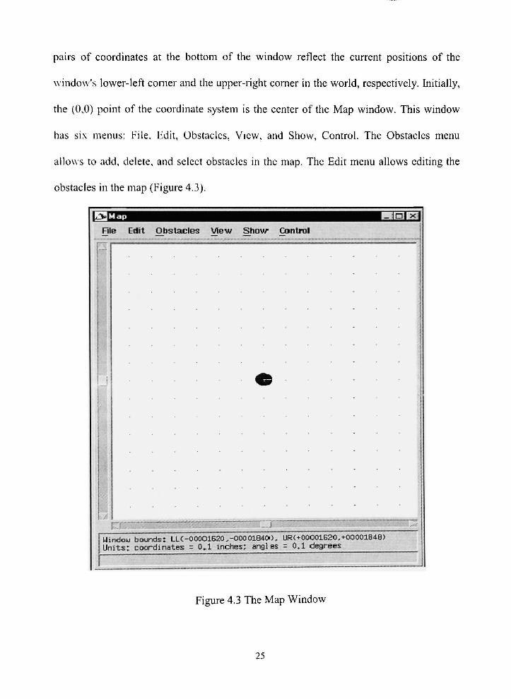
pairs of coordinates at the bottom of the window reflect the current positions of the
window's lower-left corner and the upper-right comer in the world, respectively. Initially,
the (0,0) point of the coordinate system is the center of the Map window. This window
has six menus: File, Edit, Obstacles, View, and Show, Control. The Obstacles menu
allows to add, delete, and select obstacles in the map. The Edit menu allows editing the
obstacles in the map (Figure 4.3).
RlMap Qolxl File Edit Obstacles View Show Cantrol
. J Uindou bountJs: LLC-000OlS20.-0000184«», UR<+00O01G20,1-00001848) Uni ts : cooridinates = OA inches; angles = 0.1 degrees
Figure 4.3 The Map Window
25

4.2.3 The Robot Window
The Robot window allows interactive control of a robot (Figure 4.4). This
window has five menus: Robot, View, Show, Refresh, and Panels. At the bottom of the
window are information about the current robot position, compass value, and the last
11 Robot: Nomadll)
Robot View 3hDW Refresh Panels
n X
B
Window bounds: LL(-00O0170O,-0OO0203C», UR(+0OO017OO,*0OO02i fictual p o s i t i o n : )K=+00000000 V=+O0OO0O0O S=0000 T=0000 Encoder p o s i t i o n ? X=+00000000 V=+OOOaOOOO S=0000 1=0000
CuiuHai's wdluc; OOOO Pr-ftui niJS rnmrnflnrlr t nKift yfit. Unitat cool-di no tea = 0.1 inchc i j angles = 0^1 degrees
Figure 4.4 The Robot Window
26

command issued. In position information, X and Y are the coordinates, S is the steering
direction in degrees, T is the turret direction in degrees. Note that the turret is maintained
for backwards-compatibility with older Nomad robots. On the Scout and Super Scout, the
turret always faces the same direction as the steering angle. Degrees range from 0 to 360,
with 0 as the horizontal right. The robot menu has the following options:
• Real Robot switches between the real robot and the simulator. While switching to
the real robot one should make sure that the appropriate communication (radio
modem or radio ethemet) is set up between the robot and the host computer.
• Place robot allows placing the robot in a given configuration. Synchronization
bars and handles appear as shown in Figure 4.5. Only the robot that are currently
displayed in the window according to the SHOW menu will be affected by place
robot operation. If only the Encoder robot is shown, then the Encoder position and
orientation will be reset.
Turret sync bar
Label
Axis Handles
Steering sync bar
Figure 4.5 Place Robot
27

There are some specific operations when the two robots, Encoder and Actual, are
displayed at the same time; the effects of the actions of both encoder and actual robot are
displayed in the Map window.
4.2.4 The ShoilSensors Window
The ShortSensors Window has an option menu which can display the bumpers
when the robot runs into an obstacle and Infrared sensor data as radius lines. There are
two kind of views. The local view, in which the robot's forward direction is always
aligned with the upward vertical direction of the window. The global view, in which the
robot will rotate with respect to the existing environment, as the turret of the robot
rotates.
Options
Figure 4.6 The ShortSensor Window
28

4.2.5 The LongSensors Window
The LongSensors Window has an Option menu, which can display the Sonar rays,
Sonar Cones, Sonar Connections, Laser and Robot proximity (Figure 4.7). There are two
kinds of views. The local view, in which the robot's forward direction is always aligned
with the upward vertical direction of the window; all the sensors are fixed. In global
view, the robot will rotate with respect to the environment in the Map window, as the
tun-et of the robot rotates.
,4ona, Smysz H oinafHI J'
^ t i o n s
\
V
/
I
(
V
\
Figure 4.7 The LongSensor Window
4.3 Programming the Robot
In this implementation, to run the robot, a program is used, instead of manually
sending commands to it. There are two ways to run the robot from a program.
29

• Direct mode
The program communicates directly with the robot daemon (the program constantly
running on the robot that accepts commands from outside, executes them, and sends data
back).
• Client mode
The program communicates as a client to the server: the server accepts the commands
of the program (exactly as it accepts the commands from the graphic interface) and
transmits them to the robot daemon. The server can also transmit the commands to a
simulation module of the real robot.
Application 1
Nclient.o
^
Ndirect.o
Client
-^ < - ^
Server
^
Simulator
Server
->
• ^
Robot Daemon
^ ->1 Robot
Robot
Figure 4.8 Programming in Direct and Client Mode
30

The client mode is used for testing and debugging a program. The direct mode is used
when the program is completely correct, to minimize the communication overhead. The
sample program in Figure 4.9 does the following:
Connects to the robot
Initializes it using the command zr
Sets the translational speed to 5 inches/s
Translates the robot by 100 inches (lOOOtenths of inches)
Gets the robot state during the motion
Disconnects from the robot
The include file Nclient.h contains the prototypes of the robot commands: zr,pr, etc.
31

#include "Nclient.h"
void main()
{
connect_robot(l);
zr();
sp (50, 50, 0);
pr(1000, 1000,0);
while (State[STATE_CONF_X] < 1000)
gs();
disconnect_robot( 1);
Figure 4.9. Sample program to run the robot
32

4.4 The Global Vectors
The information about the current state of the robot, its configuration and the readings
of the sensors can be obtained by an application program through a global array, called
the State vector. This structure is updated after the execution of a robot command. The
name fields are values that are defined in Nclient.h; they are used in application programs
rather than the index into the array, thus increasing the readability and is invariant to
changes in the Slate vector.
4.4.1 The State Vector
The fields of the State Vector are as follows:
STATE SIM SPEED Simulation Speed.
The value is a factor to the speed of real-time; its unit is 1/10. Therefore, 10
corresponds to real-time, with a setting of 5 the simulation of one second will take two
seconds (half the speed) and with a setting of 20 it will take 1/2 second (twice the speed).
STATE_SONAR_0- 15
The readings of the sixteen sonar. The sonar are numbered counter-clockwise
consecufively beginning with the front of the robot. The readings correspond to distances
in inches.
33

Figure 4.10 The arrangement of the Bumper Sensors
STATE_BUMPER
The readings of the bumpers. There is a total of six individual bumper sensors on the
robot that are arranged in a ring. Figure 4.10 shows their arrangement. Bumper sensor
number n is represented by the nth bit in this value of the state vector. The O"* bit is the
least significant one. A bit is set to one when the corresponding bumper is hit.
STATE_CONF_X
The integrated x-coordinate of the robot in 1/1 Os of inches with respect to the start
position. This value is reset by the commands zr and dp.
STATE_CONF_Y
The integrated y-coordinate of the robot in 1/1 Os of inches with respect to the start
position. This value is reset by the commands zr and dp.
34

ST'i TECONF STEER
The orientation of the steering in 1/lOs of degrees with respect to the start orientafion,
in the range [0; 3600]. This value is reset by the commands zr and da.
STATE_VEL_R1GHT
The velocity of the right wheel in 1/lOs of inches per second.
STATE lEL LEFT
The \elocity of the left wheel in 1/1 Os of inches per second.
STA TEJ10T0R_STA TUS
The status of the motors. The lowest two bits correspond to the two motors. The next
five bits apply to the new power management and sensing features of the robot.
STATE ERROR Error number
The state vector is updated by all robot motion and sensing commands. However, the
family of commands that starts with get only updates a part of the state vector. For
example, get_sn (get sonar) only updates the sonar readings. The command conf_cp,
which configures the compass, is an exception in that it does not affect the state vector at
all. If the user wants to force an update of the state vector, the command gsQ (get state)
can be issued.
4.5 Robot Commands
Programming a robot requires the following steps:
• Establish communication with a robot
• Initialize the robot and its sensors
35

• Repeat until done:
Send motion and sensing commands to the robot
Get motion and sensing data from the robot
• Disconnect from robot.
This illustrates the four basic classes of robot commands:
1. Communication commands to establish a connection to a robot.
2. Motion commands to move the robot and to obtain its current configuration.
3. Sensing commands to configure the sensors and to receive the sensory data.
4. Server commands to communicate with the server.
4.5.1 Communicafion Commands
The application program can connect to the server or directly to the robot. This is
determined by the object file the application is linked with. In case of Nclient.o the
connection will be established with the server and in case of Ndirect.o with the robot.
Some of the commands used are create_robot, connect_robot and disconnect robot.
4.5.2 Mofion Commands
The drive system of the robot consists of two independent axes. These axes are
the right and left wheels. The combination of these two wheel motions can produce
translational motion, rotation, or a combination of these to describe an arc. These two
axes can be controlled in two different control modes: velocity and posifion control. In
36

velocity control the goal is to maintain a given velocity, whereas position control attains
and maintains a given position relative to the current position of the robot.
For all motion commands velocities are specified in 1/1 Os of inches per second.
Positions are specified relative to the current position. All commands return TRUE upon
successful transmission to the robot, FALSE otherwise.
The format of commands which control each axis independently is (right wheel,
left wheel, unused), where the unused value should be passed as zero and ignored on
return. It is included for API backwards-compatibility with models that have three axes of
control. Some of the commands used are ac, sp,pr, mv, st and zr.
4.5.3 Sensing Commands
For each of the sensors there exists a command to configure it and another one to
obtain the readings. In general the sensory readings will be obtained with the gs
command that stores readings in the State vector. However, dedicated functions exist to
save bandwidth. Some of the commands are gs, conf_sn, confjm, getjsn and getjbp.
4.5.4 Server Commands
These commands are required by the application to be connected to a server. Called
from programs that connect directly to the robot (linking with Ndirect.o) they will have
no effect. Some of the commands used are server_is_running and quit_server.
37

CHAPTER 5
IMPLEMENTATION
The Monte Carlo Localization technique, including both sensor filters, has been
implemented and tested with different input maps of the environment. Figures 5.1 and 5.2
show the sample input maps of the robot's environment without any unknown obstacles.
G
Figure 5.1 Input Map 1
38

Figure 5.2 Input Map 2
The constant a was setup after several experiments of the localization program with these
input maps. The program consisted of the following steps:
1. Connect to the Robot
2. Initialize the Robot
3. Call MCL algorithm
4. Disconnect from the Robot.
The skeleton MCL Algorithm is shown in Figure 5.3. The following are the other
functions in the Monte Carlo Localization program with their input /output parameters
and description.
39

Void MCLAlgorithmO
{
InitSensorModelO;
InitSampleSetO;
For( ; ; )
a = GetActionReading ();
s = GetSensorReading();
If ( DistanceFilter(5))
{
If ( EntropyFilter(5)) knownObstacle = True;
}
for(/ = 0; i< SAMPLE SET SIZE; i++)
{
If ( Not knownObstacle ) newWeightsfiJ = weights[i];
Else newWeightsfiJ = SensorModel (s);
I t
fiormahzeV^ eights{SAMPLE_SET_SIZEy,
EliminateUndesiredSamplesO;
FillRemainingSamplesO;
Figure 5.3 Skeleton of MCL Algorithm
40

void InitScnsorModcliJ
This function initializes the Sensor Model by filling up the array containing the
Probability of obtaining a particular sensor reading given the distance from the closest
obstacle at that location. U takes no input parameters.
void InitSampleSct()
This function initializes the sample set of locations in the state space. It takes no input
parameters.
LOCATION GenerateRandomLocation(LOCATIONoldLocation, int nLevels)
This function generates a random location for the sample set. It takes two parameters, the
previous location around which a new location is to be generated and the number of
levels.
int EliminateUndesiredSamplesO
This funcfion eliminates all those locations from the sample set which do not make the
robot's location belief strong. It takes no input parameters.
int FillRemainingSamplesfint newSampleCount)
This function fills up the sample set with new locations after the undesired locations have
been removed. It takes the number of new samples needed as the input parameter.
41

L0C_BEL1EF Pm(SENSOR_READlNG_INDEX recentReadinglndex,
SENSOR_READINGJNDEXclosestObstaclelmk'x)
This function returns the probability that the sensor is reflected from a known obstacle.
The input parameters are the Sensor reading index and the Closest obstacle index.
LOC_BELIEF Pu(SENSOR_READING_INDEX recentReadinglndex)
This function returns the probability that the sensor is reflected from an unknown
obstacle. The input parameter is the most recent Sensor reading index.
int EntropyFilter(SENSOR_READING_INDEX recentReadinglndex)
This function filters the sensor readings based on its effect on the Weights. That is it uses
only those sensor readings which confirm the robot's current belief The input parameter
is the most recent Sensor reading index whose effect needs to be checked and accordingly
filtered or used for updation. Returns either a 1 or 0 indicating the result of filtering,
depending on the change in Entropy that is calculated.
int DistanceFilter(SENSORJ(EADINGJNDEX recentReadinglndex)
This function selects the sensor readings based on how much shorter they are than the
expected value. That is readings are selected based on their distance relative to the
distance to the closest obstacle in the map. The input parameter is the Sensor reading
index which is to be filtered. Returns either 1 or 0 indicating the result of filtering.
42

LOC_BELIEFScnsorModel(SENSOR_READING_lNDEX recentReadinglndex,
int loclndcx)
This function simulates the Sensor Model - P(s\l). \t takes the recent Sensor reading
index and the sample set location index as input parameters.
int ConnectAndlnitRobotQ
This function connects to the robot and initializes the robot. It takes no input parameters.
SENSOR_READING GetSensorReadingO
This function gets the current sensor reading from the robot. It takes no input parameters.
int GetActionReading(TRANS_READING& trans. STEER_READING& steer)
This function gets the current action reading from the robot.
int GetMinDistQ
This function is used for the wandering of the robot. Before every single movement of the
robot, this function checks if there is any obstacle very close to the robot.
SENSOR_READING GetClosestObstacleFromMap(LOCATIONlocation)
This function gets the distance of the closest obstacle at any given location. The input
parameter is the location for which the closest obstacle distance is to be found.
43

float Occupied(LOC Xx. LOC_Y v)
This function gives the occupancy information for a particular location. The inputs are
the X and y co-ordinates of the location whose occupancy needs to be found.
The Appendix has the detailed source code of the Monte Carlo Localization program.
44

CHAPTER 6
COMPARISON AND ANALYSIS
The implementation of Monte Carlo Localization presented in this thesis was
tested on 25 different world files (map) each with one to ten unknown obstacles whose
size as well as position in the map were generated randomly. Figures 6.1 and 6.2 show
t\\ 0 sample input maps with unknown obstacles.
Figure 6.1 Input Map 1 with 5 unknown obstacles
45

Figure 6.2 Input Map 2 with 3 unknown obstacles
The localization quality for analysis purposes of the data collected is defined as
the percentage of time steps during which the robot was localized (not lost). The robot is
considered to be localized when the belief in any one state is greater than its belief in all
the other states. A time step is defined as the CPU time taken for each iteration of the
MCL algorithm, which is the processing of information gathered from a pair of sensor
and action reading.
A trial of the experiment is running the MCL algorithm on a map with a fixed
number of unknown obstacles for 600 seconds with four different options:
1. No Filters
2. Only Entropy Filter
3. Only Distance Filter
4. Both Filters.
46

The data was collected and averaged over 25 trials for « = 1 to 10 unknown
obstacles. The data collected was the number of time steps during which the robot was
localized and the total number of time steps for each opfion. Figure 6.3 gives a graphical
representation of the data collected.
Performance of MCL with filters.
No Filters Entropy Filter Distance Filter Both Filters
2 3 4 5 6 7 8 9 10
Number of obstacles
Figure 6.3 Performance of MCL with Filters.
The graph shows the localization quality for MCL algorithm with and without
filters. The size and the position of the unknown obstacles were generated randomly.
Without any filter the MCL algorithm fails considerably with two or more number of
unknown obstacles in a map. It worked for some trials with two or three unknown
47

obstacles when they were placed very close to the walls in the map, which is actually not
the case in the real world where unknown obstacles can appear anywhere. Whereas any
one of the Entropy or Distance filter takes the number as high as 5 unknown obstacles.
But with both the filters together MCL algorithm performed satisfactorily for as many as
8 unknown obstacles. The size of the environment used for the experiment was 9 meters
X 9 meters approximately. For bigger environments the MCL algorithm with filters will
perform satisfactorily for greater number of unknown obstacles. The reason for this claim
is that the MCL algorithm with filters fails if the robot fails to get some valid sensor
readings consecutively, for example in a situation where unknown obstacles appear all
around the robot or a large number of unknown obstacles appear in the environment.
Figure 6.4 shows input map 2 with a large number of unknown obstacles, and Figure 6.5
shows the input map 1 with unknown obstacles all around the robot. Large-sized
environments can thus encompass greater number of unknown obstacles.
Figure 6.4 Input Map 2 with a large number of unknown obstacles
48

Figure 6.5 Input Map 1 with unknown obstacles all around the robot
This limitation of Monte Carlo Localization with fihering techniques can be taken
care of if the map is updated at regular intervals with the latest information of the robot's
environment.
The improved performance of the MCL algorithm with filtering techniques comes
with a cost. In the fixed time interval (600 seconds) used for each trial, MCL with no
filters could perform 2060 iterations, while MCL with both filters could perform only
1107 iterations. Though the two filters alone take almost as much computation time as
the MCL without filter does, it is well-worth the cost as it is rare to find a dynamic
environment with at most two unknown obstacles.
49

CHAPTER 7
CONCLUSIONS AND FUTURE WORK
This thesis reports a version of MCL, which uses filtering techniques with the
basic algorithm to make it work in highly dynamic environments. The improvements
offered by this new technique is to filter out the unexpected sensor data, coming from
unknown objects and update the position belief of the robot using only those
measurements which are with high likelihood produced by known objects contained in
the map. As a result it permits accurate localization even in densely crowded, non-static
environments.
However, if the sample set size is small, a well-localized robot might lose track of
its position just because MCL fails to generate a sample in the right location. MCL also
would fail with perfect noise free sensors. In other words, MCL with accurate sensors
may perform worse than MCL with inaccurate sensors. This finding is a bit counter
intuitive in that it suggests that MCL only works well in specific situations, namely those
where the sensors possess the "right" amount of noise. Researchers are trying Mixture-
MCL algorithm to get over this limitation. Mixture-MCL combines regular MCL
sampling with a "dual" of MCL, which basically inverts MCL's sampling process [1].
50

REFERENCES
[I] S. Thrun, D. Fox, and W. Burgard. Monte Cario localization with mixture proposal distribution. In Proceedings of the AAAl National Conference on Artificial Intelligence, Austin, TX, 2000. AAAI.
[2] D. Fox, W. Burgard, and S. Thrun. Markov localizafion for mobile robots in dynamic environments. Journal of Artificial Intelligence Research, 11:391-427, 1999.
[3] Larry D. Pyeatt. Integration of Partially Observable Markov Decision Processes and Reinforcement Learning for Simulated Robot Navigation. PhD thesis, Department of Computer Science, Texas Tech University, 1999.
[4] D. Fox, W. Burgard, F Dellaert, and S. Thrun. Monte Carlo Localization: Efficient position estimation for mobile robots. In Proceedings of the National Conference on Artificial Intelligence (AAAI), Orlando, FL, 1999. AAAI.
[5] A. Doucet, J.E.G. de Freitas, and N.J. Gordon, editors. Sequential Monte Carlo Methods in Practice. Springer Verlag, New York, 2001.
[6] J. Liu and R. Chen. Sequential Monte Carlo methods for dynamic systems. Journal of the American Statistical Association, 93:1032-1044, 1998.
[7] D.B. Rubin. Using the SIR algorithm to simulate posterior distributions. In M.H. Bernardo, K.M. an DeGroot, D.V. Lindley, and A.F.M. Smith, editors, Bayesian Statistics 3. Oxford University Press, Oxford, UK, 1988.
[8] D. Fox, W. Burgard, and S. Thrun. Active Markov Localization for mobile robots. Robotics and Autonomous Systems, 25{3-4): 195-207, 1998.
[9] W.R. Gilks, S. Richardson, and D.J. Spiegelhalter, editors. Markov Chain Monte Carlo in Practice. Chapman and Hall/CRC, 1996.
[10] S. Thrun. Bayesian landmark learning for mobile robot localizafion. Machine Learning 33{\), 1998.
[II] W. Burgard, A. Derr, D. Fox, and A.B. Cremers. hitegrating global position esfimation and position tracking for mobile robots: The dynamic Markov localization approach. In Proc. of the lEEE/RSJ International Conference on Intelligent Robots and Systems (IROS'98), 1998.
51

[12] A. Elfes. Occupancy Grids: A Probabilistic Framework for Robot Perception and Navigation. PhD thesis. Department of Electrical and Computer Engineering, Carnegie Mellon University, 1989.
[13] B. Schieic and J. Crowley. A comparison of position esfimation techniques using occupancy grids. In Proceedings of the 1994 IEEE International Conference on Robotics and Automation, pages 1628-1634, San Diego, CA, May 1994.
[14] J. Borenstein, B. Everett, and L. Feng. Navigating Mobile Robots: Systems and Techniques. A. K. Peters, Ltd., Wellesley, MA, 1996.
[15] W. Burgard, A.B. Cremers, D. Fox, D. Hahnel, G. Lakemeyer, D. Schulz, W. Steiner, and S. Thrun. Experiences with an interactive museum tour-guide robot. Artificial Intelligence, 114(l-2):3-55, 1999.
[16] I.J. Cox and J.J. Leonard. Modeling a dynamic environment using a Bayesian mulfiple hypothesis approach. Artificial Intelligence, 66:311-344, 1994.
[17] F. Dellaert, W. Burgard, D. Fox, and S. Thrun. Using the condensatton algorithm for robust, vision-based mobile robot localization. In Proceedings of the IEEE International Conference on Computer Vision and Pattern Recognition, Fort Collins, CO, 1999. IEEE.
[18] J.S. Gutmann, W. Burgard, D. Fox, and K. Konolige. An experimental comparison of localizafion methods. In Proceedings of the lEEE/RSJ International Conference on Intelligent Robots and Systems (IROS), 1998.
[19] D. Kortenkamp, R.P. Bonasso, and R. Murphy, editors. Al-based Mobile Robots: Case studies of successful robot systems, MIT Press, Cambridge, MA, 1998.
[20] W.D. Rencken. Concurrent localizafion and map building for mobile robots using ultrasonic sensors. In Proceedings of the lEEE/RSJ International Conference on Intelligent Robots and Systems, pages 2129-2197, Yokohama, Japan, July 1993.
[21] M. Vukobratovi' c. Introduction to Robotics. Springer Publisher, Berlin, 1989.
[22] R.E. Kalman. A new approach to linear fihering and prediction problems. Trans. ASME, Journal of Basic Engineering, 82: 35-45, 1960.
[23] M.A. Tanner. Tools for Statistical Inference. Springer Veriag, New York, 1993. 2"'' edifion.
52

APPENDIX
/ * * J | C * * * * * * * * * * J | < * * * * > | < * * * * * * > | C * * * * * > | C * * H ! * * * * * * * * * * * * * * * * * * * * * * * * * * * * * * * *
/* Monte Cario Localization Source Code */
/*Header files*/ /3|C}|C3|C3|C9|C!fC}|C9(C9|C3)CJfC}|C/
#include <stdio.h> #include <stdlib.h> #include <string.h> #include <math.h> #include "Nclient.h"
/^Defined from Map*/
#define MAP_MAX_X 29 #define MAP_MAX_Y 25 #define MAP_MIN_X -29 #defineMAP MIN Y -24
/* #define MAP MAX X #define MAP MAX Y #defineMAP MIN X #defmeMAP MIN Y */
8 8
-8 -9
#define MAP_OCCUPANCY_FN Occupied /* Interface With The Map: Occupancy function from Map which takes x,y location as parameters & returns the probability of Occupancy. */
#define MAP_SPATIAL_RESOLUTION 15 /* Size of each Cell */ /* Should be same as the Map Resolution */
/*Defined for MCL Implementafion*/
#define MAX_ACTUAL_READING 255 /* Maximum Sensor Range */ #define CONVERSIONF ACTOR 2.54 /* Conversion from inches to cms. */ #define MAX_SENSOR_READING 640 /* MaxActtialReading x
53

ConversionFactor. */
#define MAX_0R11:NTAT10N 360 /* Maximum orientation of the Robot */ #define SENSOR RANGE SIZE 30 /* Discrefization Size */ #define ANGULARRESOLUTION 36 /* Orientafion of each Cell */ #define M1N_BEL1EF 0.000001 /* Initial Minimal Belief of each Locafion */
#define ROBOTID 1 #define PORTNO 7019 #define SERVER "kripke"
/*Experimental Constants*/
#define Cd 0.9998 #define Cr 0.0002 #define SIGMA 3.4 #define GAMMA 0.9 #definePI 3.14
/*Type Declarations*/
typedefint LOC_X; typedefint LOC_Y; typedefint LOCT; typedef float LOC_BELIEF; typedef struct
{ LOC_X x; LOC_Y y; LOCT theta; } LOCATION;
typedef float WEIGHT; typedef long TRANS_READ1NG; typedef long STEER_READING; typedef long ACTIONREADING; typedef long SENSOR_READING; typedefint TRANS_READING_INDEX; typedef short SENSOR_READING_INDEX;
54

/*Variables Declarations*/ / l |<)|c)|ci|cHc%*>|ci|c*H(i|!*>l<:|<>l<*!|<>l<>|i/
const int nGridX = (MAP_MAX_X-MAP_MIN_X) + 1; const int nGrid_Y = (MAP_MAX_Y-MAP_MIN_Y) + 1; const int nOrientations = MAXORIENTATION / ANGULARRESOLUTION; const int nLocations = (nGrid_X * nGridY * nOrientations); const short nSensorRcadings = MAXSENSORREADING / SENSORRANGESIZE
+ 1; const int SAMPLE SETSIZE = nLocations/nOrientafions; LOCATION locafions[SAMPLE_SET_SIZE+l]; LOCATION newLocations[SAMPLE_SET_SIZE+l]; WEIGHT weights[SAMPLE_SET_SlZE+l]; WEIGHT newWeights[SAMPLl:_SET_SlZE+l]; LOCBELIEF Prob_di_given_ol[nSensorReadings] [nSensorRcadings]; LOCBELIEF Priori_Sensor_Model[nSensorReadings]; STEERREADING eff_steer=0; TRANS_READING_INDEXeff_trans_x[nOrientattons], eff_trans_y[nOrientations];
/*Funcfion Declarafions*/
int ConnectAndlnitRobotO; void MclAlgorithmO; void InitSensorModelO; void InitSampleSetO; int valid(int, int); int EntropyFilter(SENSOR_READING_lNDEX); int DistanceFilter(SENSOR_READING_lNDEX); int GetActionReading(TRANS_READING&, STEER_READING&); int UpdateEffSteerTrans(STEER_READING, TRANSREADING); int GenerateNewXOnActionReading(int, int); SENSORREADING GetSensorReadingO; SENSOR_READINGGetClosestObstacleFromMap(LOCATION); LOCBELIEF Pm(SENSOR_READING_lNDEX, SENSORREADINGINDEX); LOC_BELIEFPu(SENSOR_READlNG_INDEX); LOCBELIEF SensorModel(SENSOR_READING_INDEX, int); void NormalizeWeights(int); int DisplayPositionO; int RoundOff(float); int GetBestDirO; int GetMinDistO; float Occupied(LOC_X,LOC_Y); LOCATION GenerateRandomLocation(LOCATION, int);
55

int EliminateUndesiredSamplesO; int FillRemainingSamples(int); int RestoreSampleSetO;
/*Function Definitions*/
/* This is the main function which connects to the Robot and Initializes it */ /* and then calls the Monte Carlo Localization Algorithm. Once the Localization */ /* is complete, it disconnects from the Robot. */
int main() {
ConnectAndlnitRobotO; MclAlgorithmO; disconnect_robot(ROBOT_ID); return 1;
}
void MclAlgorithmO {
int MCL_Failed = 0; InitSensorModelO; InitSampleSetO;
for(;; ) { const int MAX_ALLOWED_SENSOR_READING = MAX_SENSOR_READING/SENSOR_RANGE_SIZE - 3;
STEER_READD4G steer; TRANS_READ1NG trans;
GetActionReading(trans, steer); if(UpdateEffSteerTrans(steer, trans) == 0) confinue; for(int i=0; i<SAMPLE_SET_SIZE; i++)
GenerateNewXOnAcfionReading(i,i);
SENSOR_READING sT = GetSensorReadingO; SENSORREADE^GESfDEX recentReadinghidex =
(SENSOR_READING_INDEX)RoundOff(((float)sT)/SENSOR_RANGE _S1ZE);
56

/* Applying Filtering Techniques. */ int knownObstacle = 0; if(recentReadinglndex < MAXALLOWEDSENSORREADING)
if(DistanceFilter( recentReadinghidex)) if(knownObstacle = EntropyFilter(recentReadinglndex))
knownObstacle - 1;
for(int i=0; i<SAMPLE_SET_SlZE; i++) {
if(!knownObstacle) newWeights[i] = weights[i];
else newWeights[i] = SensorModel(recentReadingIndex,i) * weights[i];
NormalizeWeights(SAMPLE_SET_SlZE);
int newSampleCount = EliminateUndesiredSamplesO;
if(newSampleCount == 0) { MCL_Failed = 1; break; }
if(newSampleCount < SAMPLE_SET_SIZE) FillRemainingSamples(newSampleCount);
RestoreSampleSetO; DisplayPositionO; }
if(MCL_Failed) printf("\n\n !!!... MCL failed to generate Sample at Robot true Locafion ...!!!\n\n"); return;
}
LOCATION GenerateRandomLocafion(LOCAT10N oldLocation, int nLevels)
{ LOCATION result; do { int randomlndex = rand()%9;
int randomOrient = rand()%3; int offsetX, offsetY, offsetT;
switch(randomlndex) {
case 0: offsetX=0; offsetY=0; break; case 1: offsetX=0; offsetY=l; break; case 2: offsetX=0; offsetY—1; break;
57

}
case 3: otTset,\-=l; offsetY=0; break; case 4: offsetX=l; offsetY=l; break; case 5: olTsetX =1; offsetY=-l; break; case 6: offsetX=-l; offsetY=0; break; case 7: offsetX=-l; offsetY=l; break; case 8: offsetX=-1; offsetY=-1; break;
switch(randomOrient) {
case 0: offsetT=0; break; case 1: offsetT=l; break; case 2: offsetT=nOrientations-l; break;
I
result.X = oldLocafion.x + offsetX; resuh.y = oldLocafion.y -i- offsetY; result.theta = (oldLocation.theta+offsetT) % nOrientations;
} while(!valid(result.x, nGrid_X) || !valid(result.y, nGridY));
if(nLevels > 0) result = GenerateRandomLocafion(result, —nLevels);
return result; }
/* This function eliminates all those locations from the sample set which do not make */ /* the robot's location belief strong. It takes no input parameters. */
int EliminateUndesiredSamplesO {
int newSampleCount = 0; for(int i=0; KSAMPLESETSIZE; i++) { if(newWeights[i] != 0.0) {
newLocadons[newSampleCount] = newLocafions[i]; newWeights[newSampleCount] = newWeights[i]; newSampleCount++;
} } return newSampleCount;
}
58

/* This function fills up the sample set with new locations after the undesired */ /* locations have been removed, ft takes the number of new samples needed as */ /* the input parameter. */
int FillRemainingSamples(int newSampleCount) {
int locRemaining = SAMPLE_SET_SIZE - newSampleCount; int nextFreelndex = newSampleCount; NormalizeWeights(newSampleCount); for(int i=0; i<newSampleCount; i++)
int sampleLocRemaining; if(i == newSampleCount-1) sampleLocRemaining = locRemaining; else sampleLocRemaining = RoundOff(locRemaining*newWeights[i]);
float temp = sqrt(sampleLocRemaining/3); int nLevels = (int) temp; if((temp>nLevels) || ((nLevels%2) == 0)) {
if((nLevels%2)==0) nLevels += 1;
else nLevels +- 2; } if(nLevels > 3) nLevels = (nLevels-3)/2; else nLevels = 0;
for(int j=0; j<sampleLocRemaining; j++)
{ newLocations[nextFreeIndex] =
GenerateRandomLocafion(newLocafions[i], nLevels);
newWeights[nextFreelndex] = newWeights[i]; nextFreeIndex++;
} newWeights[i] *= (sampleLocRemaining + 1); locRemaining -= sampleLocRemaining; } NormalizeWeights(SAMPLE_SET_SIZE); return 1;
}
int RestoreSampleSetO
{
59

for(int i=0; i<SAMPLE_SET_SlZE; i++) { locations[i] = newLocations[i]; weights[i] = newWeights[i]; }
/ • This function initializes the Sensor Model by filling up the array containing the */ /* Probability of obtaining a particular sensor reading given the distance from the */ /* closest obstacle at that location. It takes no input parameters. */
void InitSensorModelO {
/* Filling Prob_di_given_ol Array */
for(int i=0; i<nSensorReadings; i++) { LOC_BELIEF sumPu = (LOC_BELIEF) 0; for(int j=0; j<i; j++) sumPu += Pu(j); for(int ol=0; oKnSensorReadings; 0I++) {
LOCBELIEF sumP = (LOC_BELIEF) 0; for(int j=0; j<i; j++) sumP += Prob_di_given_ol[j][ol]; Prob_di_given_ol[i][ol] = 1 - ((1 - (l-sumPu)*Cd*Pm(i,ol))*(l - (1-
sumP)*Cr)); } } return;
}
/* This funcfion inifializes the sample set of locations in the state space, ft takes no */ /* input parameters.*/
void InitSampleSetO
{ /* Inifializing Sample Set. */
WEIGHT umformWeight = (WEIGHT) 1.0/SAMPLE_SET_SIZE ; int offset = nLocations / SAMPLE_SET_SIZE; int newLocationlndex = 0;
60

for(int i=0; i<SAMPLE_SET_SIZE; i++) { LOCT new T = newLocationlndex % nOrientations; LOCY newY = (newLocationlndex / nOrientations) % nGridY; LOC X new_X = ((newLocationlndex / nOrientations) / nGridY) % nGridX;
locations[i].x = new_X; locations[i].y = new_Y; locations[i].theta = newT;
weights[i] = uniformWeight;
newLocationlndex += offset; I I
return;
void NormalizeWeightsfint lastlndex) {
WEIGHT total = (WEIGHT) 0; for(int i=0; i<lastlndex; i+-i-) total += newWeights[i]; for(int i=0; i<lastlndex; i++) newWeights[i] /= total;
}
/* This function Updates the weights of all locations in the sample set */ /* using the most recent Acfion Reading due to translation. */ /* The input parameter is the most recent Translation Reading obtained. */
int GenerateNewXOnActionReading(int locationlndex, int newLocationlndex)
LOC_X newX; LOC_Y newY; LOC_T newT;
new_T = (locations[locationIndex].theta + eff_steer) % nOrientations; new_X = locations[locationIndex].x + eff_trans_x[new_T]; new_Y = locations [locationlndex].y + eff_trans_y[new_T];
newLocations[newLocationIndex].theta = newT; if(!valid(new_X, nGrid_X) || !valid(new_Y, nGrid_Y)) rettim -1; newLocations[newLocationIndex].x = newX; newLocations [newLocationlndex] .y = new_Y; return 1;
61
/* This function returns the probability that the sensor is reflected from a known */ /* obstacle. The input parameters are the Sensor Reading index */ /* and the Closest Obstacle index. */
LOC_BELIEF Pm(SENSOR_READING_INDEX recentReadinghidex, SENSORREADlNGlNDEXclosestObstaclelndex)
{ LOCBELIEF exponent = (recentReadinglndex - closestObstaclehidex) / SIGMA; return exp(-0.5 * exponent * exponent) / (SIGMA * 2.51);
t
/* This function returns the probability that the sensor is reflected from an */ /* unknown obstacle. The input parameter is the most recent Reading index. */
L0C_BEL1EF Pu(SENSOR_READING_INDEX recentReadinghidex) {
LOC_BELIEF sumPrevReadings = (LOC_BELIEF) 0; if(recentReadinghidex == 0) return (L0C_BEL1EF) 0; for(int i=0; i<recentReadingIndex; i++) sumPrevReadings += Pu(i); return (Cr * (1 sumPrevReadings));
/* This function filters the sensor readings based on its effect on the Weights. That is it*/ /* uses only those sensor readings which confirm the robot's current belief The */ /* input parameter is the most recent Sensor reading index whose effect needs */ /* to be checked and accordingly filtered or used for updation. Returns either a */ /* 1 or 0 indicating the result of filtering, depending on the change in Entropy */ /* that is calculated. */
int EntropyFilter(SENSOR_READING_INDEX recentReadinghidex)
{ LOCBELIEF alphaT=0.0; LOC_BELIEF prevBelief, prevEntropy = (LOC_BELIEF) 0; LOC_BELIEF currBelief, currEntropy = (LOC_BELIEF) 0;
/* Calculafing the value of alphaT */
for(int i=0; i<SAMPLE_SET_SIZE; i++) alphaT += SensorModel(recentReadingIndex,i) * weights[i];
62

/* Calculating the Entropy values */ / j l c j i t j i t H t * * * * * * * * * * * * * * * * * * * * * * * * /
for(int i=0; i<SAMPLE_SET_SIZE; i++) { LOCBELIEF newWeight = SensorModel(recentReadinglndex,i) * weights[i] / alphaT; if((weights[i] < MINBELIEF) || (newWeight < MINBELIEF)) confinue;
pre\Belief \\cights[i]; prevEntropy+= -prevBelief* log(prevBelief); currBelief = newWeight * prevBelief / alphaT; currEntropy += -currBelief * log(currBelief); }
if((currEntropy - prevEntropy) < 0) return 1; else return 0;
/* This function selects the sensor readings based on how much shorter they are than*/ /* the expected value. That is readings are selected based on their distance relative to */ /* the distance to the closest obstacle in the map. The input parameter is the */ /* Sensor reading index which is to be filtered. Retums either 1 or 0 indicating the */ /* result of filtering. */
int DistanceFilter(SENSOR_READlNG_INDEX recentReadinglndex) {
LOCBELIEF Pshort - (LOCBELIEF) 0, tmpPshort[nSensorReadings];
for(int ol=0; oKnSensorReadings; ol++)
{ tmpPshort[ol] = (LOC_BELIEF) 0; for (int l=recentReadingIndex+l; l<nSensorReadings; 1++) tmpPshort[ol] += Pm(l,ol); }
for(int i=0; i<SAMPLE_SET_SlZE; i++) Pshort += tmpPshort[RoundOff(((float)GetClosestObstacleFromMap(newLocations[i]))/SE NSOR_RANGE_SIZE)] *weights[i];
63

return (Pshort < GAMMA) ' 1 : 0;
LOCBELIEF SensorModel(SENSOR_READINGJNDEX recentReadinghidex, int loclndcx)
SENS0R_READ1NG_1NDEX ol = (SENSOR_READING_INDEX) RoundOff(((float)GetClosestObstacleFromMap(newLocafions[lochidex]))/ SENSORRANGESIZE); retum(Prob_di_given_ol[recentReadinglndex][ol]);
}
int UpdateEffSteerTrans(STEER_READING steer, TRANS_READING trans)
{ static STEERREADING steerPrevLeft=0; static float X_PrevLeft[nOrientations]; static float Y_PrevLeft[nOrientations]; int someTrans=0;
effsteer = (steer+steerPrevLeft)/ANGULAR_RES0LUT10N; steerPrevLeft=(steer+steerPrevLeft)%ANGULAR_RES0LUT10N; if(steerPrevLeft > ANGULAR_RES0LUTI0N/2)
{ eff_steer++; steerPrevLeft -= ANGULAR_RESOLUTION; }
for(int k=0; k<nOrientafions; k++)
float rad = (k*ANGULAR_RESOLUTION + steerPrevLeft)*PI / 180.0; X_PrevLeft[k] += trans*cos(rad); Y_PrevLeft[k] += trans *sin(rad); eff_trans_x[k] = (TRANS_READ1NG_INDEX) (X_PrevLeft[k] / MAP_SPATL\L_RESOLUTION); eff_trans_y[k] = (TRANS_READING_INDEX) (Y_PrevLeft[k] / MAP_SPATIAL_RESOLUTION); if((eff trans_x[k]!=0) || (eff_trans_y[k]!=0)) someTrans = 1; X Pre~vLeft[k] -= eff_trans_x[k]*MAP_SPATIAL_RES0LUT10N; YlPrevLeft[k] -= eff_trans_y[k]*MAP_SPATIAL_RES0LUT10N;
}
if((eff_steer != 0) || someTrans) rettim 1; else return 0;
64

}
int valid(int val, int maxval) {
if((val>=0) c & (val<max_val)) return 1; else return 0;
(
int RoundOfftfloat x) {
return (int) (2.0*x - (int) x); }
int DisplayPositionO I
int Localised = 0, count=0; WEIGHT max Weight = 0.0; for(int i=0; i<SAMPLE_SET_SIZE; i++) if(weights[i] > max Weight)
max Weight = weights [i];
printfi("\n "); printf("\n Robot Localized At"); for(int i=0; i<SAMPLE_SET_SIZE; i++) if(weights[i] == max Weight) {
printf(" ( %d,%d,%d ) ",locafions[i].x,locations[i].y,locafions[i].theta); if((++count % 7) == 0) printf("\n"); Localised = 1;
}
if(!Localised) printf("Not Localised.\n"); return 1;
/* This function connects to the robot and initializes the robot. It takes no */ /* input parameters. */
int CormectAndlnitRobotO {
/*SERV_TCP_PORT = PORTNO; strcpy(SERVER_MACHINE_NAME, SERVER);*/ if(!connect_robot(ROBOT_ID))rettim(0);
65

conf_tm(2); zr(); ac(200,200,0); sp( 100,100,0); return 1;
}
/* This function gets the current sensor reading from the robot. It takes no */ /* input parameters. */
SENSORREADING GetSensorReadingO I
gsO; rettim (SENSORREADING) (State[STATE_SONAR_0] * CONVERSIONFACTOR);
}
/* This function gets the current action reading from the robot. */
int GetActionReading(TRANS_READING& trans, STEER_READING& steer) {
static int oldSteer=0; static double oldTransX=0; static double oldTransY=0; double newTransX,newTransY; int newSteer;
if(GetMinDist() < 20) { int angle = GetBestDir(); gsO; ac(0,0,0); sp(50,0,0); pr(angle,0,0); st(); ws(TRUE,TRUE,TRUE,20);
} else { gsO; ac(0,0,0); sp(350,350,0); pr(59,59,0); stO;
66

ws(TRUE,TRUE,TRUE,20);
gs(); newStcer = (State[STATE_CONF_STEER]/10)%MAX_OR1ENTATION; if(oldSteer <= newSteer) steer = newSteer - oldSteer; else steer = 360 - oldSteer + newSteer;
gsO; newTransX = (State[STATE_CONF_X])*CONVERSlON_FACTOR/10.0; newTransY = (State[STATE_CONF_Y])*CONVERSlON_FACTOR/10.0; trans = RoundOff(sqrt(pow((newTransX-oldTransX),2)+pow((newTransY-oldTransY),2)));
oldTransX = newTransX; oldTransY = newTransY; oldSteer = newSteer;
return 1;
/* This function is used for the wandering of the robot. Before every single movement */ /* of the robot, this funcfion checks if there is any obstacle very close to the robot. */
int GetMinDistO {
int minvalue = 255; for(int i=0; i<3; i++) if(State[STATE_SONAR_0 + i] < min_value)
min_value = State[STATE_SONAR_0 + i];
for(int i=0; i<2; i++) if(State[STATE_S0NAR_14 + i] < min_value)
min_value = State[STATE_S0NARJ4 + i];
return min_value;
}
int GetBestDirO {
int max_value = 0, best_dir; gsO; for(int i=STATE_S0NAR_3; i<=STATE_S0NAR_13; i++)
67

if(State[i] > niaxvalue) {
max_value = State[i]; bestdir = i-STATE_SONAR_0;
I I
if(max_value >= 20) return (best_dir*225); else return -1;
}
/* This function gets the distance of the closest obstacle at any given location. The */ /* input parameter is the location for which the closest obstacle distance is to be found. */
SENSORREADING GetClosestObstacleFromMap(LOCATION location)
I /* Get closest Obstacle from Map & return the distance. */
LOC_X firstX, lastX; LOC_Y firstY, lastY; int IsFirst=l;
LOC_X obstacle_X, x; LOCY obstacleY, y; LOCT theta; X = obstacle_X = location.x; y = obstacle_Y = location.y; theta = locafion.theta; float rad = theta * ANGULAR_RESOLUTION * PE180.0; float cosTheta = cos(rad); float sinTheta = sin(rad); float tanTheta = tan(rad); int NoObstacle = 0; SENSOR_READING result; do { lastX = obstacle_X; lastY = obstacle_Y; iffcosTheta >= 0.707) {
obstacle_X++; obstacle_Y = RoundOff(tanTheta*(obstacle_X - x)) + y;
} else if(sinTheta > 0.707)
68

obstacle Y++; obstacleX = RoundOff((obstacle_Y y)/tanTheta) + x;
I
else if(cosTheta <= -0.707) I I
obstacle^—; obstacle_Y = RoundOff(tanTheta*(obstacle_X x)) + y;
I
else iftsinTheta < -0.707) ( \
obstacle_Y—; obstacle_X = RoundOff((obstacle_Y y)/tanTheta) + x;
} if(!valid(obstacle_X, nGrid_X) || !valid(obstacle_Y, nGrid_Y)) NoObstacle = 1; if(IsFirst) {
firstX = obstacleX; firstY = obstacle_Y; IsFirst = 0;
} } while(!NoObstacle && (MAP_OCCUPANCY_FN(obstacle_X+MAP_MIN_X,obstacle_Y+MAP_MIN_ Y)<0.5));
result = RoundOff(sqrt(pow(firstX-lastX,2) + pow(firstY-lastY,2))) * MAPSPATIALRESOLUTION; if(NoObstacle || (result > MAX_SENSOR_READING)) remm MAX_SENSOR_READING; else retum(result);
/* This function gives the occupancy information for a particular location. The inputs */ /* are the x and y co-ordinates of the location whose occupancy needs to be found. */
/For Input Map 2 */ /*float Occupied(LOC_X x, LOCY y) {
if(((x==MAP_MnvJ_X) II (x==MAP_MAX_X) || (y==MAP_MIN_Y) || (y==MAP_MAX_Y))
II ((x==5) && ((y<=0) && (y>=-6)))) return 1.0; else return 0.0;
69

*/
/* For Input Map 1 */ float Occupied(LOC_X x, LOC_Y y) {
if(((x==MAP_MlN_X) II (x==MAP_MAX_X) || (y==MAP_MIN_Y) (y==MAP_MAX_Y))
II (((x=-20) II (x==-21)) && ((y<-21) && (y>=-5))) II (((x==8) II (x==9)) && ((y<=9) && (y>=-18))))
return 1.0; else return 0.0;
70

PERMISSION TO COPY
In presenting this thesis in partial ftilfillment of the requnements for a master's
degree at Texas Tech University or Texas Tech University Health Sciences Center, I
agree that the Library and my major department shall make it freely available for
research purposes. Permission to copy this thesis for scholariy purposes may be
granted by the Dnector of the Library or my major professor. It is understood that
any copying or publication of this thesis for financial gam shall not be allowed
without my further written permission and that any user may be liable for copyright
infringement.
Agree (Permission is granted.)
Disagree (Permission is not granted.)
Student Signature Date