Monte Carlo Calculations of The Depth Distribution Function in Multilayered Structures

SURFACE AND INTERFACE ANALYSIS, VOL. 25, 341È351 (1997)

Monte Carlo Calculations of The DepthDistribution Function in Multilayered Structures

A. R. Jackson,1 M. M. El Gomati,1* J. A. D. Matthew2 and P. J. Cumpson31 Department of Electronics, University of York, York YO1 5DD, UK2 Department of Physics, University of York, York YO1 5DD, UK3 Division of Materials Metrology, National Physical Laboratory, Teddington, Middlesex TW11 0LW, UK

The statistical-weights Monte Carlo program of Cumpson for the calculation of depth distribution functions(DDF) has been extended in order to allow faster operation by use of a compiled language, C+ + , and thesimulation of multilayer structures. The simulation of Auger electrons originating from a homogeneously distrib-uted trace impurity has been performed for a number of thin Ðlms of di†erent thickness and atomic numbers onsubstrates of di†erent atomic number and of semi-inÐnite thickness. The DDFs from bulk copper and gold samplesand double and trilayer structures of carbon, copper and gold are presented. In both the bi- and trilayer structures itis found that the gradients of the DDF seem to switch fairly abruptly between the characteristics for each elementat the boundary. 1997 by John Wiley & Sons, Ltd.(

Surf. Interface Anal. 25, 341È351 (1997)No. of Figures : 10 No. of Tables : 1 No. of Refs : 18

KEYWORDS: depth distribution function ; electron transport ; multilayered structures ; Monte Carlo simulation

INTRODUCTION

The depth distribution of electrons escaping from asample under examination by AES or XPS is of greatimportance to the analyst, because without some know-ledge of the origin of detected electrons, quantitativeanalysis of spectra is severely limited. This can be com-plicated by the fact that electrons are usually scatteredmany times before being detected, leading to a spectrumthat depends on many factors, including the energy ofthe Auger electrons, the angle at which the electrons arecollected and the composition of the surface under test.

The behaviour of electrons impacting on a solid, andtheir simulation by Monte Carlo methods is welldescribed in the literature ;1 the electronÈsolid inter-actions can be split into two categories, elastic andinelastic. In the event of elastic scattering, electrons loseno signiÐcant amount of energy but change direction byanything up to 180¡. In the case of inelastic scattering,energy is lost by the electron but only a very smalldirection change occurs, providing that the energy loss,*E, is signiÐcantly less than the electron energy.

Although recently considerable attention has beenpaid to the importance of the spectral background,2 itwould be extremely difficult to work through thephysics required to deÐne an entire spectrum and theanalyst is normally only interested in the “no lossÏ peaksof the spectrum; these are created by electrons that havelost little or no energy between emission and detection.This information is contained within the depth distribu-tion function (DDF), which is deÐned as the probability

* Correspondence to : M. M. El Gomati.

that an electron emitted from a given depth range willreach the surface and be detected with negligible energyloss6 (i.e. loss of \500 meV).

The simplest approximation to the DDF is the so-called straight-line approximation (SLA), where elasticscattering is ignored.3 This gives rise to a simple decay-ing exponential with the inelastic mean free path as thecharacteristic length. This has been shown to be inaccu-rate for materials of large atomic number and for largeangles of emission, because elastic scattering is moreimportant under these conditions than under lowatomic number and low angles of emission. MonteCarlo simulation allows one to improve on this methodand produce more realistic results by taking intoaccount the elastic scattering properties of the materialbeing simulated ; achieving this analytically can be verycomplex.4 Conventional Monte Carlo simulations arewell known to be capable of producing results of rea-sonable reliability. However, this can be a very slowprocess due to the time taken to produce sufficientlygood statistics to provide the required signal-to-noiseratio, and hence only certain classes of analysers oflarge acceptance angles can be simulated.

The problem of the inefficiency of the direct MonteCarlo simulations has been partly overcome in the caseof calculating the DDF with the introduction of the tra-jectory reversal method by Gries and Werner.5 In thismethod, only the electrons detected by the analyser aresimulated. A further improvement to Monte Carlosimulations is the use of the statistical-weights methodsused in nuclear physics to reduce the statistical uncer-tainty associated with the direct Monte Carlo approach.This method was successfully applied by Ebel andJablonski7 to accelerate convergence of a Monte Carlosimulation of XPS emission. Cumpson6 has combined

CCC 0142È2421/97/050341È11 $17.50 Received 16 September 1996( 1997 by John Wiley & Sons, Ltd. Accepted 16 January 1997

342 A. R. JACKSON, M. M. EL GOMATI, J. A. D. MATTHEW AND P. J. CUMPSON

the trajectory reversal method with the statistical-weights techniques and in so doing has shown theadvantage of combining these two approaches in calcu-lating the DDF.

The method described by Cumpson was originallywritten using the MATLAB numerical computationpackage but has been converted into the C]] lan-guage so that accurate results can now be achieved inunder 1 min on a personal computer, representing morethan a tenfold increase in speed. This improvement hasbeen achieved due to the fact that C]] is a compiledlanguage that has inherent advantages over the inter-preted MATLAB package, such as improved speed,portability and Ñexibility, allowing the incorporation ofan intuitively easy user interface.

Further to this, the program has been extended inorder to produce DDFs for heterogeneous structures.Firstly, the simple case of a single overlayer to thesample has been studied in order to assess the value ofsuch an investigation before more complex samplegeometries are considered. The program is thenextended to look at the DDFs produced by a trilayerstructure. Agreement of these programs with the orig-inal published results of Cumpson for homogeneousmaterials is extremely good.

The basic parameters required for any of these simu-lations are the inelastic mean free path (IMFP) and thedi†erential elastic scattering cross-sections, leading toboth the elastic mean free path (EMFP) and the trans-port mean free path (TMFP). The mean free path isdeÐned by Committee E-42 on Surface Analysis of theASTM (American Society for Testing and Materials) as :“the average distance that an electron travels in-betweentwo successive collisions of the speciÐed typeÏ.8 Thevalues for the IMFP used here are taken from the workof Tanuma et al.,9,10 who produced IMFP data for 27elements in the range 50È2000 eV.

The Mott elastic scattering cross-sections, derived bypartial wave expansion, are used in all the Monte Carlowork presented here and give a better approximation totrue electron behavior than alternatives such as theRutherford cross-section.11 The data used here aretaken from the work of Czyzewski et al.,12 who pro-duced a comprehensive database of di†erential cross-sections for 94 elements in the range 20È30 keV.

The work presented here extends the work ofCumpson to allow simulation of samples consisting ofbi- and trilayer geometries, and involves only thestatistical-weights method. The more analyticalapproach of Berger and Doggett was not used becausein this method the electron trajectories are not explicitlydeÐned, making it much more difficult to take intoaccount the e†ects of heterogeneous structures on theelectronÏs behaviour. Many recent publications havehighlighted the need for an understanding of electronbehaviour in multilayer heterogeneous samples, and inmany cases this work is related to the overlayer methodfor experimentally determining the attenuationlength.13h15

Werner16 also addressed the issue of overlayers insimulations leading to the production of DDFs, but thiswork di†ered from that presented here in some keyways. Firstly, Werner looked only at signal electronsproduced by the substrate and overlayer individually,giving rise to discontinuous DDFs. This is intuitively

obvious in that particular study because there will be noAuger electrons characteristic of the substrate actuallyproduced in the overlayer, and vice versa. The simula-tions presented here correspond to those electrons orig-inating from a homogeneously distributed traceimpurity (such as a dopant), or any source emitting atenergies in the range 50È2000 eV for which elastic andinelastic scattering data for both overlayer and sub-strate are available. Further, the work here is based onthe trajectory reversal and statistical-weights work ofCumpson as mentioned above, so that a personal com-puter can be used to produce good results in a fewminutes, as opposed to hours using conventionalmethods.

The structures examined here include bilyaer samplesof carbon, copper and gold in various combinations,and trilayer samples of carbon and gold. Transporttheory equations have been used to validate the resultsproduced by the Monte Carlo programs and giveencouraging results ; also, the Monte Carlo results aresuccessfully compared to analytical predictions of elec-tron behaviour at large depths.

THE MODEL

The statistical-weights method : the bilayer model

Since full details of the model are given by Cumpson,6we will only present here the basic steps of the statisticalweights process and highlight the modiÐcations made inthe present work.

The method used here is a reverse-trajectory,statistical-weights procedure. The simulated electronsoriginate at the analyser, enter the surface and undergoscattering events according to the same prescription asa conventional simulation. According to the reverse tra-jectory technique, the positions of the Ðrst inelastic scat-tering events in this type of simulation give the samedepth distribution as a forward Monte Carlo approach.

The step lengths are chosen according to the formula

Step \ [je ln(R) (1)

where R is a random number between 0.0 and 1.0 andis the elastic mean free path.je Applying the statistical-weights method, we can iter-

atively accumulate the probability distributions for theÐnal depths, (where i is the iteration number),r

i(z)

rather than explicitly calculating the depth of eachinelastic scattering event as it occurs in the simulation.The method used for producing for any given pathr

i(z)

is as follows :From the di†erential elastic scattering cross-section

data of the atoms in the sample, angles and intervals forthe elastic scatterings in the simulation . . . nf1, f2 , f3 ,are randomly sampled. This gives us a set of depths ofpolar direction of motion . . . at which(h1, /1), (h2, /2),the elastic scattering events occur and a set of anglescorresponding to each scattering event, etc. This part ofthe calculation is identical to a conventional Monte

( 1997 by John Wiley & Sons, Ltd. SURFACE AND INTERFACE ANALYSIS, VOL. 25, 341È351 (1997)

MONTE CARLO CALCULATION OF DDF IN MULTILAYERED STRUCTURES 343

Figure 1. Schematic showing the structure used in the trilayersimulations.

Carlo simulation, and the details are described byShimizu and Ding.11

The next step is to calculate the electron Ñuence, fk(z),

between the kth and (k ] 1)th elastic scattering, for aunit electron Ñux incident on the surface. This Ñuence isproportional to the probability of an Auger electronbeing successfully detected, having originated at a depthz and undergone k elastic scattering events

f0(0)\ 1o cos h0 o

(2)

Becauase all the scattering events we are looking at areelastic (and therefore involve no loss of energy), we mustconserve Ñuence between successive line segments of thepath

fk(f

k)

o cos hko\ f

k~1(fk)o cos h

k~1o(3)

giving the electron Ñuence as

fk(z) \

G fk(f

k)exp[[(z[ f

k)/j

icos h

k]/o cos h

ko

0(4)

the upper condition being satisÐed if min(fk, f

k`1) \and being zero otherwise. Thisz\max(fk, f

k`1), fk(z)

gives us the result

ri(z) \ ;

0

qfk(z) (5)

where q is set as the maximum number of scatteringevents that will be considered for any given electronpath. For the purpose of the calculations in the twoprograms presented, this was set to 20, because this willalmost certainly yield at least one inelastic scattering ineach electron path.

In order to take into account the presence of an over-layer, the mean free paths used in Eqns (1) and (4) mustbe adjusted according to the materials in which the elec-tron has travelled. Further to this, the mean free pathused in the calculation to determine the event of aninelastic scattering will now depend on the electronÏshistory.

The position of the electron is normally described inspherical polar coordinates, taken from one elastic scat-

tering to the next. This is satisfactory for homogeneoussamples but is rather complicated when layered struc-tures are involved. In this case, to simplify the calcu-lations necessary when the boundary is crossed, theseare converted into Cartesian coordinates at every stepof the electron trajectory. The equations used are thesame as those described by Shimizu and Ding11 in theirreview of Monte Carlo modelling

xn`1\ x

n] s

n(sin 0

ncos /

n) (6)

yn`1\ y

n] s

n(sin 0

nsin /

n) (7)

zn`1\ z

n] s

n(cos 0

n) (8)

where and represent the new electronxn`1, y

n`1 zn`1coordinates, and are the starting coordinates,x

n, y

nzn

snis the current step length and and are the angles0

n/

ngiven in polar coordinates of the new electron position.The single interface condition required to model

bilayers is handled by resetting the electron position tothe point at which it crossed the interface and then con-tinuing the simulation as normal, having adjusted theparameters accordingly. The remaining step after theelectron has been returned to the boundary is calculatedby referring to the formula used in the original steplength calculation

Step \ [je0 ln(R) (9)

where R is a random number and is the elastic meanje0free path of the starting material for the transition. Theremaining step is then calculated as follows

Remaining–step \ [je1 ln(R) (10)

where both R are di†erent simple trigonometry allowsus to calculate the distance to the boundary as(L b)

L b\ J(xb[ x0)2] (yb[ y0)2] (zb [ z0)2 (11)

Where and are the electronsÏ coordinates at thexb , yb zbboundary.

Trilayer simulation

The transition from bilayer to trilayer is much morestraightforward than that from homogeneous to bilayersimulation, since the routines for identifying the posi-tion of each electron in three-dimensional space arealready in place. This development is, however, by nomeans trivial because we now have to deal with con-siderably more possible outcomes of a single electrontransition. The electron can cross no boundary, crossone boundary only or cross both boundaries.

Dealing with a single boundary crossing is handledusing the same method as described for the bilayer case.If both boundaries are crossed, then crossing of the Ðrstboundary is handled as with the Ðrst case, but the elec-tron then continues from this position as if it has under-gone an elastic scattering event with no directionchange. For simplicity, the trilayer simulation at presentsimulates structures consisting of a layer of thickness aof element Za over a layer of thickness b of element Zbfollowed by the bulk material Za, but could easily beadapted to cope with more complex situations. This isschematically depicted in Fig. 1.



RESULTS

Comparison with existing published results

The Ðrst stage in this section will deal with validatingthe results of the overlayer simulation program by com-paring them with those produced by the MATLABscript, which has already been validated by Cumpson.

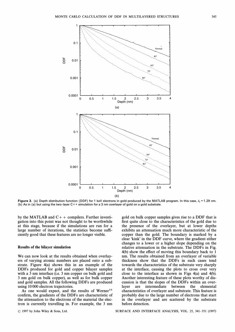
To this end, simulations were carried out on copperand gold for a variety of angles of emission using hypo-thetical layers of the same element as the substrate (e.g.gold on gold or carbon on carbon), which should yieldthe same results as the bulk simulation. Gold andcarbon have been chosen to give conÐdence that theprogram is reliable over a range of atomic numbers.Results for 7000 electron trajectories of 1000 eV are pre-sented in Figs 2 and 3. Figures 2(a) and 3(a) representthe MATLAB results for carbon and gold, respectively,

Figures 2(b) and 3(b) represent the C]] simulationsdescribed above. It can be seen that there is very littlediscrepancy between the results from the two programs.This is encouraging, particularly when considering thedi†erent manner in which the programs operate. Thesuccess of these tests is useful not only to show that theMATLAB methods of Cumpson have been successfullytranslated into C]], but also to give conÐdence in theboundary crossing handling routines used, because weexpect a two-layer simulation of gold on gold, orcarbon on carbon, to give the same results as for thehomogeneous case.

The most obvious di†erence between DDFs pro-duced by the two di†erent programs is the presence ofthe sharper, positive-going spikes on the MATLABresults. These are particularly noticeable during theearly stages of convergence of the routines, and couldpossibly be attributed to either the di†erent randomnumber generators used in the simulations or to dis-crepancies in the numerical precision of routines used

(a)

(b)

Figure 2. (a) Depth distribution function (DDF) for 965 eV electrons in carbon produced by the MATLAB script of Cumpson. Here, theinelastic mean free path is 2.63 nm. (b) The same simulation as in (a) but carried out using the C½½ program for a 3 nm layer of carbon(l

i)

on a bulk carbon substrate.



(a)

(b)

Figure 3. (a) Depth distribution function (DDF) for 1 keV electrons in gold produced by the MATLAB program. In this case, nm.li¼1.29

(b) As in (a) but using the two-layer C½½ simulation for a 3 nm overlayer of gold on a gold substrate.

by the MATLAB and C]] compilers. Further investi-gation into this point was not thought to be worthwhileat this stage, because if the simulations are run for alarge number of iterations, the statistics become suffi-ciently good that these features are no longer visible.

Results of the bilayer simulation

We can now look at the results obtained when overlay-ers of varying atomic numbers are placed onto a sub-strate. Figure 4(a) shows this in an example of theDDFs produced for gold and copper bilayer sampleswith a 3 nm interface (i.e. 3 nm copper on bulk gold and3 nm gold on bulk copper), as well as for bulk copperand gold samples. All the following DDFs are producedusing 10 000 electron trajectories.

As one would expect, and the results of Werner16conÐrm, the gradients of the DDFs are characteristic ofthe attenuation to the electrons of the material the elec-tron is currently travelling in. For example, the 3 nm

gold on bulk copper samples gives rise to a DDF that isÐrst quite close to the characteristics of the gold due tothe presence of the overlayer, but at lower depthsexhibits an attenuation much more characteristic of thecopper than the gold. The boundary is marked by aclear “kinkÏ in the DDF curve, where the gradient eitherchanges to a lower or a higher slope depending on therelative attenuation in the substrate. The DDFs in Fig.4(b) show the e†ect of moving this boundary back to 1nm. The results obtained from an overlayer of variablethickness show that the DDFs in such cases tendtowards the characteristics of the substrate very sharplyat the interface, causing the plots to cross over veryclose to the interface as shown in Figs 4(a) and 4(b).Another interesting feature of these plots worthy of dis-cussion is that the slopes of the DDFs within an over-layer are intermediate between the elementalcharacteristics of overlayer and substrate. This feature isprobably due to the large number of electrons that startin the overlayer and are scattered by the substratebefore detection.



(a)

(b)

Figure 4. (a) Depth distribution functions (DDFs) for 1 keV electrons at normal exit angle produced by copper with a 3 nm gold overlayer,and gold with a 3 nm copper overlayer—the DDFs from the bulk substrates are shown for comparison, is 1.29 nm for gold and 1.63 nml

ifor copper. (b) The DDFs for 1 keV electrons produced at normal exit angle from copper with gold overlayers, and gold with copperoverlayers. The boundary has been reduced to 1 nm.

We can now examine the e†ects of a bilayer structureinvolving two materials very di†erent in atomicnumber. Figure 5 shows this with a structure consistingof 3 nm overlayers of carbon and gold, again for 1000eV electrons. As one would expect, the changes in gra-dient of the DDFs produced are more pronounced inthe carbonÈgold plots than the copperÈgold DDFsshown in Figs 4(a) and 4(b) due to the large di†erence inelectron scattering for the two materials. The highatomic number substrate does not produce an enhance-ment in the gradient of the overlayer DDF at the inter-face due to direct backscattering of electrons. It isinteresting to note that Werner16 was also unable toobserve such changes in the DDF near the interface of asystem comprising a thin Be overlayer on a gold sub-strate.

Examination of Fig. 5 reveals the presence of a smalldiscontinuity in the DDF at the point of the boundary.This has been shown to be a result of the precision

attainable by the depth sampling in the present simula-tion. This was demonstrated by doubling the number of“bins per nmÏ from 20 to 40, giving a subsequentimprovement in the smoothness of the DDF around thepoint of the boundary. The results shown here are allproduced with 40 points per nm.

A close inspection of Fig. 5 reveals that the probabil-ity of escape for electrons in the carbon overlayer wassubstantially reduced as a result of the bulk gold under-neath. Figure 6(a) is a further investigation into thispoint, and shows DDFs for a sample consisting of avarying thickness of carbon on a bulk gold.

Examination of Fig. 6(a) shows that the slope of theDDFs in the carbon region does gradually movetowards that of the bulk carbon, but is still signiÐcantlydi†erent even when the thickness of carbon is quitelarge (e.g. 8 nm in the last plot). Figure 6(b) shows theDDFs produced with the interchanging of the materialsused in the structure examined above. In this case, at



Figure 5. Depth distribution functions (DDFs) produced from overlayers of carbon and gold for 1 keV electrons at normal exit angle. TheDDFs for the bulk substrates are shown for comparison.

(a)

(b)

Figure 6. (a) The effect of varying thicknesses of carbon overlayers on bulk gold on the depth distribution function (DDF) at normalemission for 1 keV electrons. (b) The DDFs produced for 1 keV electrons in carbon, with overlayers of gold of various thicknesses.



the interface between the two materials, rather than asharp change in gradient as exhibited in the carbon-on-gold samples, the DDF appears to tend towards acarbon characteristic much more gradually. AsWerner13 pointed out in his study of the DDFs pro-duced by overlayer systems, electrons produced close tothe interface in the substrate of a weak/strong scatteringsystem are more likely to be detected than those fromthe same region in a strong/weak system. it is thereforeno surprise that features in the vicinity of the interfaceare more pronounced in the case of a carbon overlayersystem.

Reducing the kinetic energy of the simulated elec-trons to 200 eV and repeating the simulations carriedout for Fig. 5 gives rise to the results shown in Fig. 7.Now the DDFs all fall with much sharper gradientsthan in the case of the 1 keV electron simulations dueboth to enhanced elastic scattering and the reducedinelastic mean free path. It is interesting to note how theoverlayer curves deviate from the corresponding ele-mental curves at depths well below the thickness of theoverlayer. This is evidence of the importance ofredirection of electrons below the overlayer.

Results of the trilayer simulation

As with the bilayer simulation, we must Ðrst satisfy our-selves that the trilayer program is behaving as we wouldexpect in the cases for which we have data available forcomparison. To this end, single- and double-layer simu-lations were carried out using the trilayer program andcompared with the results already obtained in previousruns. Figure 5 was reproduced perfectly using the tri-layer program, simulating bilayer results by setting oneof the boundaries to zero.

An interesting test of the way in which these multi-layer simulations handle boundary crossings is to use ahomogeneous structure made up from various trilayerthicknesses of material of the same atomic number.Figure 8 shows this for samples of carbon and gold with1 keV electrons. All DDFs are produced for grazingangles of emission (80¡), as this condition is most likelyto show up any problems due to the more prominent

inÑuence of elastic scattering on the DDFs. Various“sandwichÏ structures yield identical DDFs, within theattainable statistical precision, for both carbon andgold.

We can now go on to look at the DDFs producedfrom a trilayer simulation involving two materials dif-fering in atomic number. Again, carbon and gold havebeen chosen because they exhibit such a di†erence inelastic scattering characteristics. Figure 9(a) shows theDDFs produced for “sandwichÏ layers of 3 nm and 5 nm.

For comparison, the same simulation was repeatedwith the materials in the structure reversed. The resultsof this are shown in Fig. 9(b). Again, the small spikesappearing at the boundaries are due to the mathemati-cal precision of the graphs and the lower backscatteringbehaviour of carbon. It is worth noting that for higheratomic numbers (e.g. gold and copper combinations)these spikes do not appear.

The trilayer simulations show very similar character-istics to the bilayer calculations in that the gradients ofthe DDFs seem to switch between the characteristics foreach element fairly abruptly at the boundary. As notedin the bilayer case, however, the gradient of the carbonoverlayer is substantially greater than one would expectfrom a bulk sample of the overlayer material : note thatone might expect an increased statistical probability ofemission in a carbon overlayer in the presence of a goldsubstrate, due to the high backscattering coefficient ofgold, although the lower energy inelastic mean free pathin the gold will inhibit exit of electrons that are emittedinto the crystal, without loss of energy. A carbon inter-mediate layer [Fig. 9(b)] leads to an enhanced DDF forgold emission in both the overlayer region and the sub-strate region below the carbon.

As for all the previous simulations, the transitionfrom carbon to gold is much sharper than from gold tocarbon. This feature may be attributed to the back-scattering probability from gold being so much higherthan that of carbon.

Both the bilayer and trilayer programs have beencompiled under UNIX, and give indistinguishableresults from the DOS versions used in this report. Thisindicates that the results are not heavily a†ected by thechoice of random number generator, because the

Figure 7. Depth distribution functions (DDFs) produced from overlayers of carbon and gold for 200 eV electrons. Note that is 0.88 nm.li



Figure 8. Depth distribution functions (DDFs) for the 1 keV electrons using homogeneous samples consisting of multilayer structures ofcarbon and gold.

(a)

(b)

Figure 9. (a) Trilayer simulation results for 1 keV electrons at normal incidence, together with a schematic diagram showing the structureused in the simulation. (b) The depth distribution functions (DDFs) produced from the inverse of the structure represented in (a).



random number generator used in the DOS version ofC]] is completely di†erent to that used on the UNIXcompilers.

COMPARISON WITH TRANSPORT THEORY

The Monte Carlo programs presented here yield depthdistributions that obey an exponential law for electronsoriginating from great depths. The characteristic lengthof this exponential function is given by the attenuationparameter (AP), a quantity shown by transport theoryto depend on two parameters : the inelastic mean freepath (IMFP) and the transport mean free path (TMFP).We now attempt to validate the Monte Carlo resultsusing the attenuation parameter described by Tougaardand Sigmund4 and revisited by Werner and Tilinin17when they used the so-called attenuation parameter tocompare Monte Carlo calculation with transporttheory.

The attenuation parameter is given by17ja

ja \ ji jtrji jtr

l0 (12)

where is the only positive root of the characteristicl0equation in the case of isotropic scattering

1 \ ul2

lnl] 1l[ 1

(13)

and u is the single scattering albedo

u\ jiji] jtr

(14)

The transport mean free path is calculated from thejtrMott scattering cross-sections according to the follow-

ing integral relationship

jtr~1\ 2nnP0

n dpd)

(1 [ cos h)sin h dh (15)

where n is the number of atoms per m3. The inelasticmean free path data are those of Tanuma, Powell andPenn9,10 as used in the Monte Carlo simulations them-selves.

Applying the above equations to the case of 1 keVelectrons in carbon and gold yields attenuation param-eters of 2.45 nm for carbon and 0.84 nm for gold. Figure8 gives us an attenuation parameter of 2.44 nm for 1keV electrons in carbon (0.4% discrepancy from thetheoretical prediction) and 0.81 nm for the same simula-tion arried out on gold (3% discrepancy from the trans-port theory results).

Turning to the trilayer simulation gives us some moreinteresting results. Figure 10 shows four DDFs pro-duced by the trilayer simulation. For comparison of theDDF gradient and the attenuation parameter to bevalid, we must examine the results produced by elec-trons at great depths, i.e. electrons for which thememory e†ect is not signiÐcant. Unfortunately this maybe more difficult to achieve in the presence of a “sand-wichÏ layer. The gradients of interest to us are asfollows : the gradients of the bulk materials, the gra-dients of the buried layers, and Ðnally the gradients ofthe bulk substrates. The e†ective attenuation param-eters for each region are listed in Table 1.

Bearing in mind the calculated values for as 2.45janm for carbon and 0.84 nm for gold, examination of theresults in Table 1 immediately reveals a very signiÐcantdiscrepancy between the transport theory attenuationparameters for bulk materials and the e†ective attenu-ation parameters for each section of this trilayer struc-ture.

This discrepancy is likely to be due to the fact thatthe no-memory condition has not been met, particularlyin the case of the underlayers. When dealing only withbulk materials, a normal incidence simulation yields a

Figure 10. Trilayer depth distribution functions (DDFs) for 1 keV electrons at normal angle of emission, together with the relevant DDFsfrom a bulk sample of each material used. In both of the trilayer simulations shown the interfaces are at 2 nm and 7 nm.



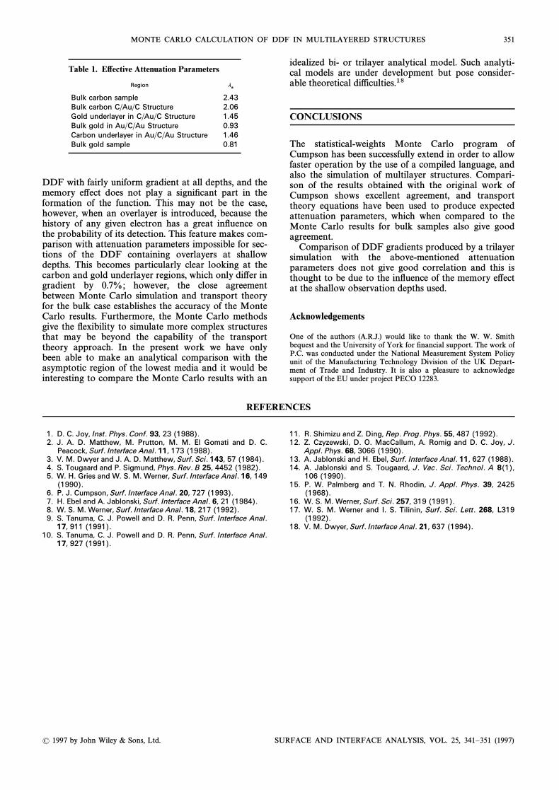
Table 1. E†ective Attenuation Parameters

Region la

Bulk carbon sample 2.43

Bulk carbon C/Au/C Structure 2.06

Gold underlayer in C/Au/C Structure 1.45

Bulk gold in Au/C/Au Structure 0.93

Carbon underlayer in Au/C/Au Structure 1.46

Bulk gold sample 0.81

DDF with fairly uniform gradient at all depths, and thememory e†ect does not play a signiÐcant part in theformation of the function. This may not be the case,however, when an overlayer is introduced, because thehistory of any given electron has a great inÑuence onthe probability of its detection. This feature makes com-parison with attenuation parameters impossible for sec-tions of the DDF containing overlayers at shallowdepths. This becomes particularly clear looking at thecarbon and gold underlayer regions, which only di†er ingradient by 0.7%; however, the close agreementbetween Monte Carlo simulation and transport theoryfor the bulk case establishes the accuracy of the MonteCarlo results. Furthermore, the Monte Carlo methodsgive the Ñexibility to simulate more complex structuresthat may be beyond the capability of the transporttheory approach. In the present work we have onlybeen able to make an analytical comparison with theasymptotic region of the lowest media and it would beinteresting to compare the Monte Carlo results with an

idealized bi- or trilayer analytical model. Such analyti-cal models are under development but pose consider-able theoretical difficulties.18

CONCLUSIONS

The statistical-weights Monte Carlo program ofCumpson has been successfully extend in order to allowfaster operation by the use of a compiled language, andalso the simulation of multilayer structures. Compari-son of the results obtained with the original work ofCumpson shows excellent agreement, and transporttheory equations have been used to produce expectedattenuation parameters, which when compared to theMonte Carlo results for bulk samples also give goodagreement.

Comparison of DDF gradients produced by a trilayersimulation with the above-mentioned attenuationparameters does not give good correlation and this isthought to be due to the inÑuence of the memory e†ectat the shallow observation depths used.

Acknowledgements

One of the authors (A.R.J.) would like to thank the W. W. Smithbequest and the University of York for Ðnancial support. The work ofP.C. was conducted under the National Measurement System Policyunit of the Manufacturing Technology Division of the UK Depart-ment of Trade and Industry. It is also a pleasure to acknowledgesupport of the EU under project PECO 12283.

REFERENCES

1. D. C. Joy, Inst . Phys.Conf . 93, 23 (1988).2. J. A. D. Matthew, M. Prutton, M. M. El Gomati and D. C.

Peacock, Surf . Interface Anal . 11, 173 (1988).3. V. M. Dwyer and J. A. D. Matthew, Surf . Sci . 143, 57 (1984).4. S. Tougaard and P. Sigmund, Phys.Rev.B 25, 4452 (1982).5. W. H. Gries and W. S. M. Werner, Surf . Interface Anal . 16, 149

(1990).6. P. J. Cumpson, Surf . Interface Anal . 20, 727 (1993).7. H. Ebel and A. Jablonski, Surf . Interface Anal . 6, 21 (1984).8. W. S. M. Werner, Surf . Interface Anal . 18, 217 (1992).9. S. Tanuma, C. J. Powell and D. R. Penn, Surf . Interface Anal .

17, 911 (1991).10. S. Tanuma, C. J. Powell and D. R. Penn, Surf . Interface Anal .

17, 927 (1991).

11. R. Shimizu and Z. Ding, Rep. Prog. Phys. 55, 487 (1992).12. Z. Czyzewski, D. O. MacCallum, A. Romig and D. C. Joy, J.

Appl . Phys. 68, 3066 (1990).13. A. Jablonski and H. Ebel, Surf . Interface Anal . 11, 627 (1988).14. A. Jablonski and S. Tougaard, J. Vac. Sci . Technol . A 8(1),

106 (1990).15. P. W. Palmberg and T. N. Rhodin, J. Appl . Phys. 39, 2425

(1968).16. W. S. M. Werner, Surf . Sci . 257, 319 (1991).17. W. S. M. Werner and I. S. Tilinin, Surf . Sci . Lett . 268, L319

(1992).18. V. M. Dwyer, Surf . Interface Anal . 21, 637 (1994).


Monte Carlo Calculations of The Depth Distribution Function in Multilayered Structures

Documents

Transcript of Monte Carlo Calculations of The Depth Distribution Function in Multilayered Structures