Monopolistic Competition in General Equilibrium: Beyond the CES∗

Evgeny Zhelobodko† Sergey Kokovin‡ Mathieu Parenti§ Jacques-François Thisse¶

23rd March 2011

Abstract

We propose a general model of monopolistic competition and derive a complete characterization

of the market equilibrium using the concept of Relative Love for Variety. When the RLV increases

with individual consumption, the market generates pro-competitive effects. When it decreases, the

market mimics anti-competitive behavior. The CES is a borderline case. We extend our setting

to heterogeneous firms and show that the cutoff cost decreases (increases) when the RLV increases

(decreases). Last, we study how combining vertical, horizontal and cost heterogeneity affects our

results.

Keywords: monopolistic competition, additive preferences, love for variety, heterogeneous firms.

JEL Classification: D43, F12 and L13.

∗We are grateful to S. Anderson, K. Behrens, E. Dinopoulos, R. Feenstra, R. Ericson, P. Fleckinger, C. Gaigné, A. Gorn,J. Hamilton, E. Helpman, J. Martin, G. Mion, T. Holmes, F. Mayneris, G. Ottaviano, P. Picard, V. Polterovich, R. Romano,

O. Shepotilo, O. Skiba, D. Tarr, M. Turner, X. Vives, S. Weber, D. Weinstein, and H. Yildirim for comments and suggestions.

We gratefully acknowledge the financial support from CORE, the Fonds de la Recherche Scientifique (Belgium), and the

Economics Education and Research Consortium (EERC) under the grant No 08-036 (with the cooperation of the Eurasia

Foundation, USAID, the World Bank, GDN, and the Government of Sweden).†Novosibirsk State University (Russia). Email: ezhel@ieie.nsc.ru‡Novosibirsk State University and Sobolev Institute of Mathematics (Russia). Email: skokovin@math.nsc.ru§Université de Paris 1 and PSE (France). Email: mathieu.parenti@gmail.com¶CORE-UCLouvain (Belgium), Paris School of Economics and CEPR. Email: jacques.thisse@uclouvain.be

1

1 Introduction

Monopolistic competition has been used successfully in a wide range of fields, including economic growth

and development, international trade, and economic geography. Although the CES utility model has

been has been extremely useful in various fields, it is fair to say that this model suffers from major

drawbacks. First, individual preferences lack flexibility since the elasticity of substitution is constant and

the same across varieties. Second, the market outcome is not directly affected by the entry of new firms.

In particular, markups and prices are independent from the number of competitors. This runs against

empirical evidence, which suggests that firms operating in bigger markets have lower markups (Syverson,

2007). Third, there is no scale effect, that is, the size of firms is independent of the number of consumers,

which contradicts the fact that firms tend to be larger in larger markets (Campbell and Hopenhayn, 2005).

Fourth, and last, firms’ price and size are independent from the geographical distribution of demand. Yet,

it is well documented that firms benefit from being closer to their larger markets, while distance accounts

for more than half of the overall difference between large plant and small plant shipments (Head and

Mayer, 2004; Holmes and Stevens, 2010).

Thus, we find it both meaningful and important to develop a more general model of monopolistic

competition. The CES must be a special case of our setting to assess how our results depart from those

obtained under the CES. Moreover, in order to provide a better description of real world markets than

the CES, our setting must also be able to cope with issues highlighted in oligopoly theory, such as the

impact of entry and market size on prices and firm size. Developing such a general model and studying

the properties of the market equilibrium is the main objective of this paper. To achieve our goal, we

assume that preferences over the differentiated product are additively separable across varieties. However,

unlike Dixit and Stiglitz (1977) who work mainly with a power function, we derive the properties of the

market outcome for a general and unspecified utility function. Though still restrictive, we will see that

additive preferences are rich enough to describe a range of market outcomes much wider than the CES. In

particular, this setting will allow us to deal with various patterns of substitution through the relative love

for variety, that is, the elasticity of the marginal utility. When consumption is the same across varieties,

the relative love for variety is the inverse of the elasticity of substitution across varieties.

Though ignoring explicit strategic interactions, our general equilibrium model of monopolistic com-

petition is sufficiently rich (i) to display several effects highlighted in industrial organization and (ii)

to uncover new results under general and well-behaved utility functions, which have empirical appeal.

Specifically, we show that the market outcome depends on how the relative love of variety varies with

2

the consumption level. To be precise, the market outcome may obey two opposite patterns. On the one

hand, when the relative love for variety increases with individual consumption, the equilibrium displays

the standard price-decreasing effects generated by the entry of new firms and a larger market size, two

effects that the CES does not capture: more firms, a larger market size, or both lead to lower market

prices because the elasticity of substitution increases. On the other hand, when the relative love for variety

decreases, the market generates price-increasing effects, that is, a larger number of firms, a bigger market,

or both lead to higher prices because the elasticity of substitution now decreases. Although at odds with

the standard paradigm of entry, this result agrees with several recent contributions in industrial organiza-

tion (Amir and Lambson, 2000; Chen and Riordan, 2007, 2008) as well as with empirical studies showing

that entry or economic integration may lead to higher markups (Ward et al., 2002; Badinger, 2007). It

should not be viewed, therefore, as an exotica. In other words, our paper adds to the literature the idea

that what looks like an anti-competitive outcome need not be driven by defence or collusive strategies: it

may result from the nature of preferences with well-behaved utility functions. In this respect, our analysis

provides a possible rationale for contrasted results observed in the empirical literature (see also Section

2.3). As expected, a higher income generates effects similar to those obtained when market size grows.

Consequently, our model involves a variable elasticity of substitution, the value of which is determined at

the market equilibrium. How this value is determined depends on the behavior of the relative love for

variety.

We also want to stress that the CES is the dividing line between the above-mentioned two classes

of utility functions since it does not display any of the effects discussed in the preceding paragraph. In

addition, we show that our main results can be extended to a multi-sector economy under fairly mild

assumptions on the upper-tier utility. Therefore, they can be used as an alternative to the CES, which is

often used in empirical trade papers. Note also that our analysis is consistent with the idea that, though

most sectors of the economy are probably pro-competitive, a few may mimic anti-competitive behavior.

Last, it is worth stressing that the relative love for variety need not be monotone, in which case our results

are locally valid only. In this event, the market outcome may display different behaviors depending on

the consumption level.

The foregoing analysis is developed in the case of homogeneous firms. Yet, there is mounting evidence

that firms are heterogeneous in terms of productivity (see, e.g. Bernard et al., 2003). It is, therefore,

natural to ask whether our modeling strategy can cope with heterogeneous firms à la Melitz (2003).

This is what we accomplish in Section 4 where it is shown that both the cutoff cost and markup decrease

(increase) with the size of the market when the relative love for variety increases (decreases) with individual

3

consumption. Under the same circumstances, the aggregate productivity rises or falls. All of this is to

be contrasted with the CES where the market size has no impact on these variables. We thus find it

fair to say that the distinction between the price-increasing and price-decreasing cases made above for

homogeneous firms keeps its relevance when firms are heterogeneous. In addition, the results are obtained

for a general distribution of marginal costs. Last, the nature of our main results still holds in a unified

framework that explicitly combines vertical, horizontal and cost heterogeneity.

Our research strategy has also empirical appeal because it provides theoretical predictions that are

sufficiently simple to be tested, sufficiently general to make sense on an empirical level, and precise enough

to allow one to discriminate between different explanations. Furthermore, our approach also sheds new

light on models that are commonly used in the empirics of trade. In particular, our analysis shows

that a single market equilibrium, which leads to a specific value of the elasticity of substitution, can be

rationalized by a CES model yielding this equilibrium. However, this does not mean that the CES can be

used without questioning its relevance in studies comparing several markets and/or periods. Indeed, even

when the CES provides a good approximation of preferences for a particular dataset, one may expect very

different estimates of the elasticity of substitution to be obtained with different ones. We need not assume

changing preferences to rationalize this difference. It is sufficient to assume that elasticity of substitution

across varieties varies with the consumption level.

The idea of additive preferences is not new since it goes back at least to Houtakker (1960), who

introduced this specification precisely because it provides new impetus to empirical analysis. Using the

same preference structure, Spence (1976) and Vives (1999, ch.6) have derived equilibrium conditions

similar to ours. However, their main purpose is different from what we accomplish in this paper since

their aim is to compare the free entry equilibrium and the social optimum. Our model also share several

similarities with Krugman (1979) who shows how decreasing demand-elasticity yields what we call price-

decreasing effects. However, Krugman did not explore the properties of the market outcome, perhaps

because his purpose was different from ours. His approach has been ignored in subsequent works by

trade theorists. As observed by Neary (2004, p.177), this is probably because Krugman’s specification of

preferences “has not proved tractable, and from Dixit and Norman (1980) and Krugman (1980) onwards,

most writers have used the CES specification.” Instead, we show that Krugman’s approach is tractable.

To be precise, by using the concept of relative love for variety, we can provide a complete characterization

of the market outcome and of all the comparative statics implications in terms prices, consumption level,

outputs, and mass of firms/varieties.

The paper is organized as follows. The next section presents the model in the case of a one-sector

4

economy. We characterize the market equilibrium when (i) the mass of firms is exogenous and (ii) the

mass of firms is determined by free entry and exit. In Section 3, our results are extended to a multi-

sector economy. In Section 4, we apply our approach to the case of heterogeneous firms and show that

the behavior of the relative love for variety is critical for the determination of the cutoff cost, thereby for

the average productivity of the industry. We build on these results to show which qualities are selected

by the market when vertically differentiated attributes are added to varieties. Section 5 shows how our

modeling strategy can be extended to the case of non-additive utilities such as the quadratic and the

translog. Section 6 concludes.1

2 The one-sector economy

2.1 The model

The economy involves one differentiated good and one production factor - labor. There are workers

and each supplies efficiency units of labor. The unit of labor is chosen as the numéraire so that

is both a worker’s income and expenditure. The differentiated good is made available as a continuum

of horizontally differentiated varieties indexed by ∈ [0 ]. They are provided by monopolisticallycompetitive (hereafter, MC) firms. Each firm produces a single variety and no two firms sell the same

variety. To operate every firm needs a fixed requirement 0 and a marginal requirement 0 of labor,

so that the production cost of a firm supplying the quantity is equal to + .

Preferences. Consumers’ preferences are additively separable. Given a (measurable) price function

p = ≤ and an expenditure value , every consumer chooses a (measurable) consumption function

x = ≤ to maximize her utility subject to the budget constraint:

max()

U ≡Z

0

()d s.t.

Z

0

d =

where (·) is a thrice continuously differentiable on (0∞), strictly increasing and strictly concave func-tion.2

The assumptions made on the utility imply that consumers are variety-lovers. Let 0 be any

given quantity of the differentiated good. If a consumer owns the same number units of each variety

∈ [0 ] with , she enjoys the utility level given by U(;) = () + ( − )(0). Note

1After completion of this paper, Kristian Behrens brought to our attention the paper by Bertoletti et al. (2008). Their

analysis starts from the same premises us but falls short of what we accomplish here.2We do not include firms’ profits into the budget constraint because total profits are zero when the mass of firms is

determined by free entry. Furthermore, being negligible to the market, a firm cannot manipulate aggregate profits.

5

that (0) 6= 0 implies that increasing the number of varieties affects the consumer’s well-being even whenshe does not change the range of varieties she consumes. This does not strike us as being plausible. For

this reason, we assume from now on that (0) = 0. That said, it is readily verified that () is a

strictly increasing function of . Consequently, rather than concentrating her consumption over a small

mass of varieties, the consumer prefers to spread it over the whole range of available varieties ( = ).

Furthermore, since the second derivative of () with respect to is negative, a consumer values

variety at a decreasing rate.

All of this has the following implication: individual consumption in the theory of monopolistic compet-

ition with love for variety is formally equivalent to individual decision-making in the Arrow-Pratt theory

of risk aversion, the mix of risky assets being replaced with the mix of differentiated varieties. This

will allow us to derive properties of firms’ demands that are both intuitive and simple. More precisely,

the key-concept for our study of monopolistic competition is what we call the relative love for variety

(hereafter, RLV), which is invariant under a linear transformation of (recall that (0) = 0):

() ≡ −00()

0() 0 (1)

Under the CES, we have () = where is a constant such that 0 ≤ 1, thus implying a

constant RLV given by 1 − . Another example is Behrens and Murata (2007) who retain the CARA

utility () = 1− exp(−) where 0 is the absolute love for variety. Thus, the corresponding RLV,

given by , increases with the consumption level.

To better understand the economic meaning of the RLV, it turns out to be useful to evaluate it along

the diagonal in the quantity space ( = ). Using the definition of the elasticity of substitution (Nadiri,

1982, p.442), we obtain

() = 1() (2)

Thus, at a symmetric consumption pattern, the RLV is the inverse of the elasticity of substitution across

varieties. However, unlike the CES where the elasticity of substitution is exogenous and constant, the value

of varies here with the consumption level or, equivalently, with the price level and the mass of varieties,

as in the translog utility (Feenstra, 2003). In other words, a higher consumption of the differentiated

product makes consumers’ love for variety stronger (weaker) when the RLV is increasing (decreasing). This

is because consumers’ preferences for more balanced bundles of varieties become stronger (weaker). Both

schemes seem a priori plausible, which means that it is hard to make predictions about the behavior of the

RLV without appealing to empirical studies. On the other hand, (2) ceases to hold when the consumption

6

pattern is asymmetric because the expression for the elasticity of substitution is more involved.

Last, observe that additive preferences with (0) = 0 are (globally) homothetic if and only if () = .

By using a general utility function , we thus obviate one of the main pitfalls encountered in many

applications of the CES.

Demand. To determine the equilibrium consumption, we differentiate the Lagrangian

U +

µ −

Z

0

d

¶

with respect to and get

0() = (3)

where the Lagrange multiplier

=

R 0

0()d

varies with the consumption function (·), the mass of varieties , and the expenditure .Clearly,

() = 0() (4)

is the inverse demand function. Because the Lagrange multiplier acts only as a scaling factor, this

expression implies that the inverse demand and the marginal utility display the same properties. In

particular, () is strictly decreasing in because is strictly concave. Unlike Dixit and Stiglitz

(1977), we do not assume that , hence , takes on a specific functional form. Furthermore, as stressed

by Vives (1999), one of the main distinctive features of monopolistic competition is that economic agents’

decisions are based on a few aggregate statistics of the distribution of firms’ actions, which they treat

parametrically. Here a single statistic, i.e. the marginal utility of income, is sufficient for firms and

consumers to make their decision.

It is readily verified that the price-elasticity of demand for a variety is equal to the inverse of the RLV

evaluated at the consumption level:

() ≡ −

=

1

[()] (5)

Therefore, a stronger (weaker) love for variety generates less (more) elastic demands. This is because a

stronger love for variety induces consumers to focus more on a balanced mix of varieties, which in turn

makes the demands for these varieties less sensitive to changes in their relative prices. This relationship

7

builds the link with Krugman (1979) who assumes the price-elasticity to be decreasing, i.e. the RLV to

be upward sloping.

Since there is a continuum of varieties, the consumption level of variety has a negligible impact on

a consumer’s utility, which implies that changing variety ’s price does not affect the demand for variety

6= . As a result, the cross-price elasticity of demand for a variety is zero, and thus this demand depends

only upon the variety price and the marginal utility of income. Furthermore, (2) and (5) imply that,

along the diagonal in the quantity space, the elasticity of substitution among varieties is equal to the

price-elasticity of a variety’s demand, as in the CES case (Vives, 1999). However, unlike the CES, this

relationship ceases to hold off-diagonal, while both and vary with the common consumption level .

Producers. Since all consumers face the same multiplier, the functional form of the demand for

variety is the same across consumers, which implies that the market demand is given by . Being

negligible to the market, each firm accurately treats as a parameter. However, as shown by (4), for

choosing its profit-maximizing output it must anticipate the equilibrium value of . Having done this,

a firm behaves like a monopolist on its market, and thus maximizing profits with respect to price or

quantity yields the same equilibrium outcome.

The marginal production cost is identical across firms. Admittedly, this assumption simplifies our

analysis because it allows us to focus on a symmetric market outcome. Therefore, one may legitimately

ask how our setting can accommodate heterogeneous firms à la Melitz (2003). We address the case of

heterogeneous firms in Section 4

Using (4), the producer’s program is as follows:

max

(;(·)) =∙0()(·) −

¸ −

For any given , the first-order condition may be rewritten as follows:

0() + 00() = (6)

where stands for the consumption level of any variety. If the conditions

lim→0

[0() + 00()] =∞ lim→∞[

0() + 00()] ≤ 0 (7)

hold, then the intermediate value theorem implies that (6) has a positive solution regardless of the value

8

of ≥ 0.3 Furthermore, if a firm’s profit function is strictly concave, (6) has a unique solution and thisone is a profit-maximizer. The strict concavity of is equivalent to

0() = −000()

00() 2 (8)

In words, this condition implies that (inverse) demands are not “too” convex.

We make an additional mild assumption on utility. It is well known that the strict concavity of profits

means that the marginal revenue is strictly decreasing. Consequently, two cases may arise. First, the

equation 0() + 00() = 0 has no solution. Using (7), it must be that () is smaller than 1 for all

0. Second, 0() + 00() = 0 has a solution 0, which is unique. In this event, we have () 1

for 0 and () 1 for 0. Therefore, we may restrict ourselves to the interval (0 0) since

the equilibrium belongs to (0 0). Without loss of generality, we may then assume that () 1 for all

relevant values of 0. To rule out the possibility of a market outcome in which firms sell an arbitrarily

small quantity at an arbitrarily high price, we assume (0) 1. In sum,

() 1 for all ≥ 0 (9)

Therefore, at a symmetric equilibrium the elasticity of substitution exceeds 1. Throughout the rest of

this paper, we assume that conditions (7)-(9) are satisfied.

To disentangle the various effects at work, it is both relevant and convenient to distinguish between

what we call a short-run equilibrium, in which the mass of firms is fixed, and a long-run equilibrium

in the which the mass of firms is endogenously determined through free entry and exit. Because the

short-run analysis is an intermediate step in the study of the long-run equilibrium where profits are zero,

we do not address the impact of the redistribution of profits.

2.2 The short-run equilibrium

Let ≡ be firm ’s output. Given the mass of firms, ≤ is a short-run equilibrium if no firm

finds it profitable to change unilaterally its output while anticipating accurately the value of . For any

given , (8) implies that (6) has a single solution . Since all firms face the same Lagrange multiplier, the

solutions to these first-order conditions are the same across firms, i.e. = for (almost) all ∈ [0 ].Thus, if a short-run equilibrium exists, it must be symmetric. It is denoted by = (). Let be the

3These two conditions are sufficient but not necessary. For example, 1 = 2√+ 1 − 2 used below does not satisfy (7)

but yields a unique profit-maximizer.

9

resulting equilibrium price.

It is readily verified that the first-order condition for firm ’s profit maximization may be written as

follows:

≡ −

= () (10)

Hence, in equilibrium, the markup of a firm is equal to the RLV. Since () 1, the elasticity of

substitution must exceed 1 at any symmetric equilibrium. Furthermore, the budget constraint implies

that the two equilibrium conditions are given by

=

1− () =

(11)

The existence and uniqueness of a short-run equilibrium are established in Appendix A.

The impact of . Differentiating the equilibrium condition (11) with respect to leads to the

expression

= − 0

(1− )2

µ

2+

2

¶

Multiplying this expression by and using = yields after rearrangements

(1− + 0)

= −0 (12)

It follows from (A.1) in Appendix 1 that 1− + 0 0. Therefore, (12) implies that and 0()

have opposite signs. Consequently, we have:

Proposition 1 If (7)-(9) hold, then there exists a unique and symmetric short-run equilibrium. Fur-

thermore, when the relative love for variety increases (decreases) with the consumption level, then the

equilibrium price decreases (increases) with the mass of firms. The equilibrium price is independent of the

mass of firms if and only if the utility is given by a CES.

To understand the intuition behind this proposition, note that the equilibrium consumption of each

variety decreases with because expenditure is distributed over a wider range of varieties, while price

change do not outweigh this impact. More precisely, since 1, it follows from (12) that the elasticity

of with respect to exceeds −1. Differentiating the equilibrium condition = with respect to

then implies that decreases.

We are now equipped to discuss the results of Proposition 1. When the RLV increases with the

consumption level, the entry of new firms leads to a lower equilibrium price. This is the standard price-

10

decreasing effect generated by entry, which works here as follows. Since the individual consumption level

decreases with , () also decreases, thereby raising the elasticity of substitution (). Varieties are

then better substitutes after entry, which makes the market more competitive and yields lower prices. In

this event, preferences generates a price-decreasing effect. By contrast, when the RLV decreases with the

consumption level, the entry of new firms leads to a price hike. In other words, though firms behave non-

cooperatively, preferences are such that the market gives rise to a price-increasing effect. This unexpected

result can be explained by reversing the above argument. Because the individual consumption decreases

with , entry now decreases the value of (), and thus varieties become more differentiated. The market

is, therefore, less competitive, which results in a higher market price. The CES is the only function that

has a constant RLV. Consequently, the CES is the only utility for which entry does not impact on the

equilibrium price. Hence, we may safely conclude that the CES is the borderline between two different

classes of utility functions, which give rise to price-decreasing or price-increasing effects. Intuitively, entry

shifts down demands but the effect on price is ambiguous. Specifically, it depends on demand’s curvature

or, equivalently, on the behavior of the elasticity, which is here equal to the RLV. According to Proposition

1, whether the market mimics pro-competitive or anti-competitive behaviors depends on the curvature of

varieties’ demand relative to the curvature of the CES-demand.

To illustrate, consider the class of “generalized Hyperbolic Absolute Risk Aversion” utility functions:

() =1

[(+ ) − ] + (13)

where ≥ 0, 0, ≥ 0, and 0 1. This expression boils down to the CES for = = 0. Setting

(i) = 1, = 1, = 0, = 12, and (ii) = 0, = 1, = 1, = 12 in (13), we get

1() = 2√+ 1− 2 2() = 2

√+

which imply

1() =1

2(1 + 1)2() =

1

2(1 +√)

Clearly, 1() increases with whereas the 2() decreases, which means that the market outcome is

price-decreasing under 1 and price-increasing under 2. For simplicity, we have chosen to express the

equilibrium prices through their inverse () for = 1 2 in which is normalized to 1. Under 1, we

have

(1) =2− 1

21(1 − )

11

which is decreasing in 1 over ( 2), so that 1() also decreases with . Under 2, we obtain

(2) =4(2 − )2

2(2 − 2)2

which is also defined over ( 2). Differentiating this expression shows that (2) is increasing on this

interval, whence 2 increases with .

2.3 The long-run equilibrium

A symmetric long-run equilibrium is defined by a mass of firm and a symmetric equilibrium such

that firms earn zero profits:

(− ) = (14)

This shows that the equilibrium outcome depends on the “relative” market size ≡ , so that com-

parative statics in terms of allows one to capture shocks in both population and technology. Using (14)

and the budget constraint, we obtain

=

=

1

Using this expression and (10) yields the equilibrium consumption of each variety:

=1

µ1

− 1¶ (15)

Furthermore, The conditions for a long-run equilibrium may then be written as follows.

Proposition 2 Every symmetric long-run equilibrium must satisfy the following two conditions:

=

∙1

µ1

− 1¶¸

(16)

= (17)

The existence and uniqueness of a long-run equilibrium under (7)-(9) can be proved as in Section 2.2.

In particular, since the equilibrium markup is bounded, the equilibrium mass of firms is always finite. To

illustrate, we return to the utilities 1 and 2 used the above examples and determine the corresponding

12

markups:

1 =2p

8+ 1 + 32 =

1

2

Ã1− 1p

+ 1

!

It is readily verified that 1 and 2, respectively, decrease and increase with .

2.3.1 The impact of cost and market size

Markup. Totally differentiating (16) with respect to = , solving for and multiplying both

sides by , we obtain the elasticity:

E ≡

= −

+0

0 = − (1− )

(1− ) + 00 = −

(1− )

(2− 0) 0 (18)

=( − 1)(2− 0)

0 = ( − 1)1 + − 0

2− 0 − 1 (19)

where we have used successively (15), (16), the identity 0 ≡ (1 + − 0), (12), and (9).

Using (16) yields the elasticities

E ≡

=

= −

=

≡ E (20)

Since 1 and 0 2, it follows from (18) that and 0 have opposite signs. Therefore, as in

Section 2.2, three cases may arise according to the sign of 0. For example, when 0 0, the equilibrium

markup decreases with . As a result, the equilibrium price falls when the population size increases,

the level of fixed cost decreases, or both. These effects are expected because a larger or a smaller

fosters entry, which here leads to a lower market price. This corresponds to the standard price-decreasing

effect generated by a bigger market. In contrast, when 0 0, we fall back on the price-increasing effect

uncovered in the above section.

We show in Appendix B that a higher marginal cost always leads to a higher price. In addition, 0 0

(0 0) implies that a higher marginal cost leads to a less (more) than proportional increase in market

price. In other words, the pass-on varies with the RLV.

Industry size. To study how the size of the MC-sector changes with , we differentiate the equilib-

rium condition (17). Using (19), we then obtain

= 1 +

0

13

Hence, regardless of the sign of 0, the equilibrium mass of firms is always an increasing function of the

size of the economy. Thus, the RLV does not affect the pro-entry effect generated by a larger market.

However, it affects the way this pro-entry effect reacts to market size: the above elasticity is smaller

than 1 if and only if 0 0, which means that () grows at a decreasing rate. In other words, when

consumers display an increasing (decreasing) RLV, a growing population enjoy a larger but less (more)

than proportionate mass of varieties. As it should now be expected, the mass of varieties grows linearly

with if and only if the utility is given by the CES.

How does react to the cost parameters? Since increasing is tantamount to decreasing , must

decrease with . Furthermore, as shown in Appendix B, a higher marginal cost leads to a larger mass of

firms if and only if 0 0.

Consumption and output. The impact of the above parameters on and can be obtained in a

similar way by differentiating the corresponding equilibrium conditions (see Appendix B for more details).

It is worth to single out two results. First, the consumption of each variety always falls when the size of

the economy rises, the reason being that consumers prefer to spread their consumption over the wider

range of varieties that results from the entry of new firms. Second, despite the larger mass of competitors,

a growing population induces each firm to produce more if and only if the RLV is increasing. Again, this

is because the entry of new firms leads to a lower market price.

2.3.2 Synthesis

Our results may be summarized in the following two propositions.

Proposition 3 The impact of the relative market size e ≡ on the symmetric long-run equilibrium

is as follows:

0() 0 0() = 0 0() 0

E ≡

↓ : − E 0 : E = 0 ↑ : 0 EE ≡

↑ : 0 E 1 ↑ : E = 1 ↑ : 1 E

E ≡

↓ : −1 E 0 ↓ : E = −1 ↓ : E −1E ≡

↑ : 0 E 1 : E = 0 ↓ : E 0

Again, we see that what determines the properties of the market outcome is the variety-loving attitude

of consumers. That said, the following comments are in order. First, regarding the impact of the relative

market size on the equilibrium price, it is worth noting that the long-run equilibrium inherits the price-

14

decreasing and price-increasing properties of the short-run equilibrium. To understand why, we observe

that the size of the industry always grows with . Indeed, when there are more consumers, the profits

of incumbents increase, thus attracting new firms. According to the sign of 0, such an entry leads to a

lower or higher market price. When 0 0, the decrease in market price slows down the entry of new

firms. However, since the elasticity of with respect to is smaller than 1, this negative feedback effect

cannot outweigh the initial increase in . Consequently, the market price is established at a level lower

than the initial one. On the contrary, when 0 0, the feedback effect is positive. This further pushes

upward, making the elasticity of bigger than 1, which in turn yields a higher market price. Yet, this

price does not become arbitrarily large because the individual consumption of each variety decreases at

a rate exceeding 1. Under the CES, there is no feedback effect because the market price is unaffected by

the entry of new firms. Thus, using the CES as a benchmark, when the market size grows, consumers

face a smaller range of varieties and lower prices when they display an increasing RLV. In contrast, the

range of varieties is wider and prices are higher under a decreasing RLV than under the CES.

To shed further light on the role of market size, it is worth investigating how the equilibrium value

of the Lagrange multiplier changes with . It follows immediately from (6) that

=0()[1− ()]

=

0() + 00()

Differentiating the numerator of this expression and using (8) shows that strictly decreases with .

Therefore, regardless of , a larger economy generates a higher marginal utility of income. This a priori

unsuspected result may be explained as follows. While consumers buy a large amount of each variety

in a small economy, they buy a smaller amount in a large economy because they face a wider range of

varieties. This lower consumption makes income more valuable in the large economy than in the small

one.

Another peculiar feature of the CES is that the equilibrium size of firms () is independent of the

market size. Our results show that firms’ size increases in the price-decreasing case. This is because the

industry size grows at a lower pace than the market size while prices go down. On the contrary, firms’

size decreases when the price-increasing effect prevails because the mass of firms rises at a more than

proportionate rate, while prices go up. These effects combine to yield a lower output. This provides a

possible reconciliation between diverging results in empirical analysis. For example, Holmes and Stevens

(2004) observe that the correlation sign between firm and market sizes differ in services and manufacturing,

whereas Manning (2010) finds a robust correlation between average firm size and total labor market size.

15

Proposition 3 shows that the sign of the correlation between these two variables depends on the nature

of preferences, and thus may vary across goods as well as with their technology since lowering fixed costs

is equivalent to raising market size.

The impact of marginal cost is less straightforward and is obtained in Appendix B.

Proposition 4 The impact of marginal cost on the long-run symmetric equilibrium is as follows:

0() 0 0() = 0 0() 0

E ≡

↑ : 0 1− E 1 ↑ : E = 1 ↑ : 1 EE ≡

↓ : −(1− ) E 0 : E = 0 ↑ : 0 E

E ≡

↓ : −1 E 0 ↓ : E = −1 ↓ : E −1E ≡

↓ : −1 E 0 ↓ : E = −1 ↓ : E −1

Using (18) and (20) when preferences generate price-decreasing (price-increasing) effects, the markup

decreases (increases) because the market price increases less (more) than proportionally. This in turn

fosters the exit (entry) of firms. Consequently, a technological change affects the degree of diversity

in opposite directions. This discrepancy in results should be useful in empirical studies to distinguish

between the two competition regimes. By contrast, in the CES case, increasing the marginal cost leaves

the markup unchanged.

In addition, under CES preferences, consumers always benefit from a larger market because prices re-

main constant while more varieties are available. This positive size effect is reinforced the price-decreasing

effect because prices go down while the market supplies more varieties. Hence consumers are better-off.

In the price-increasing case, the impact of market size on welfare is not so clear. Indeed, although more

varieties are still available, they are priced at a higher level. Therefore, if the equilibrium price increases

at a much higher rate than the mass of varieties, one may expect the welfare level to decrease with the

size of the market. And, indeed, we have found well-behaved utility functions such that a growing market

size is detrimental to consumers.

2.3.3 Income and preferences

Assume that consumers have more resources, and thus the individual expenditure is higher. Inspecting

(16) shows that the equilibrium price is independent from . This is because the price-elasticity of a

firm’s demand depends only upon the RLV prevailing in the MC-sector. It then follows from (17) that

the equilibrium mass of firms is an upward-sloping linear function of . In other words, increasing either

16

or leads to a larger mass of firms. Note, however, that the two parameters describing the size of

the sector, i.e. and , do not play exactly the same role in determining the market outcome: is

independent of , whereas varies with . Note also that the elasticity of substitution () increases

(decreases) with the income when is an increasing (decreasing) function because a higher income

invites more entry, which in turn reduces the level of consumption of each variety.

We now study how the market outcome reacts to a stronger love for variety, that is, the RLV takes

on a higher value for all ≥ 0. Let

() ≡ −

∙1

µ1

− 1¶¸

be defined on [0 1]. Repeating the argument used to show the existence and uniqueness of a short-run

equilibrium, it is readily verified that () is strictly increasing on [0 1] and such that (0) 0 and

(1) 0, while the equation () = 0 has a single solution. Therefore, when is shifted upward, ()

moves downward, and thus the equilibrium markup increases. Using (17) shows that the equilibrium mass

of firms also increases. In sum, a stronger love for variety endows firms with more market power, bringing

a higher price and more variety.

Before moving to the case of a multi-sector economy, we want to make a pause and discuss further the

relevance of the CES in empirical works using the monopolistic competitive setting. In equilibrium, the

RLV is equal to the inverse of the elasticity of substitution. Consequently, one can rationalize the use of

the CES once the value of () = 1() evaluated at the market outcome is known. In other words, for

any symmetric long-run equilibrium obtained within our framework, there exists a CES model that yields

the same market outcome. Yet, this does not mean that the CES can be used doubtlessly in empirical

analyses. In order to estimate a model with cross-section or panel dataset, we need data heterogeneity

stemming from variations in the underlying structural parameters such as the relative market size .

Once we allow for such variations, Proposition 3 tells us that the corresponding elasticity of substitution

also changes, except in the special case in which the real world would be described by the CES. All of

this has the following major implication: it is likely to be meaningless to assume that the elasticity of

substitution is the same across space and/or time (Broda and Weinstein, 2006, and Head and Ries, 2001,

among many others). This should not be interpreted as a negative message, however. Instead, it is our

contention that richer functional forms, which encompasses both price-increasing and price-increasing

effects, should be used in empirical analyses. The results in Proposition 3 provide some guidelines that

should help empirical economists in detecting whether or not the market is price-decreasing, thereby

17

helping them to choose a particular specification. To the very least, we find it fair to say that our analysis

gives credence to such an alternative modeling strategy.

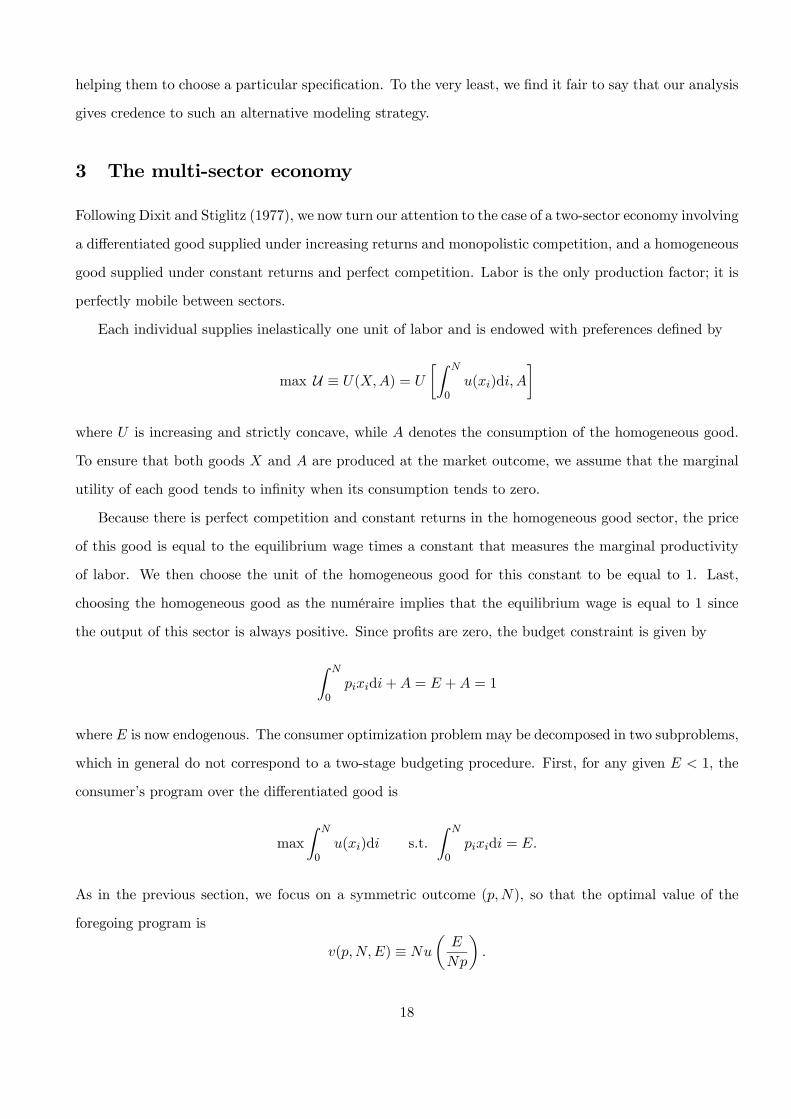
3 The multi-sector economy

Following Dixit and Stiglitz (1977), we now turn our attention to the case of a two-sector economy involving

a differentiated good supplied under increasing returns and monopolistic competition, and a homogeneous

good supplied under constant returns and perfect competition. Labor is the only production factor; it is

perfectly mobile between sectors.

Each individual supplies inelastically one unit of labor and is endowed with preferences defined by

max U ≡ () =

∙Z

0

()d

¸

where is increasing and strictly concave, while denotes the consumption of the homogeneous good.

To ensure that both goods and are produced at the market outcome, we assume that the marginal

utility of each good tends to infinity when its consumption tends to zero.

Because there is perfect competition and constant returns in the homogeneous good sector, the price

of this good is equal to the equilibrium wage times a constant that measures the marginal productivity

of labor. We then choose the unit of the homogeneous good for this constant to be equal to 1. Last,

choosing the homogeneous good as the numéraire implies that the equilibrium wage is equal to 1 since

the output of this sector is always positive. Since profits are zero, the budget constraint is given by

Z

0

d+ = + = 1

where is now endogenous. The consumer optimization problem may be decomposed in two subproblems,

which in general do not correspond to a two-stage budgeting procedure. First, for any given 1, the

consumer’s program over the differentiated good is

max

Z

0

()d s.t.

Z

0

d =

As in the previous section, we focus on a symmetric outcome (), so that the optimal value of the

foregoing program is

() ≡

µ

¶

18

The function is the indirect utility level derived from consuming the differentiated good at the symmetric

outcome. It follows from the properties of that is decreasing and convex in , increasing in , increasing

and concave in , while the cross-derivatives satisfy 00 0 and 00 0.

Second, the upper-tier maximization problem may be written as follows:

max

(() 1−)

in which () is the index of the differentiated good consumption. Let () be the unique solution

to the first-order condition

01(·)0(·) = 02(·) (21)

evaluated at a symmetric outcome (). Hence, the lower-tier optimization problem becomes

max

Z

0

()d s.t.

Z

0

d = ()

Hence, when consumers preferences are described by a general two-tier utility (·), the properties of are immaterial for the value of the equilibrium price. To illustrate, consider a Cobb-Douglas utility,

i.e. () = log + (1− ) log. When is the CES, the expenditure function is given by the

share of total income. This ceases to hold when is not the CES. To determine (), let = 0

denote the elasticity of the lower-tier utility with respect to consumption. After some manipulations

the first-order condition (21) yields

1−

=1−

0 =

1−

()

where denotes the long-run equilibrium consumption of every variety. Using (15) shows that ()

depends only upon , which is itself the unique solution to (16). Therefore, () is independent of , so

that the equilibrium expenditure on the differentiated good is defined by

() =[()]

(1− )+ [()]

This expression is tractable enough to be used in comparative static analyses for many specifications of

the lower-tier utility embodied in a Cobb-Douglas upper-tier utility.

On the other hand, when is unspecified, it is not possible to derive a closed-form expression for

. However, we are able to derive the main properties of the long-run equilibrium under some mild

19

assumptions on and . First, since the equilibrium price , individual consumption and firm’s output

prevailing in the MC-sector are independent of the value of (see (16)), their properties still hold

within this general setting.

In contrast, the characterization of the equilibrium mass of varieties is more involved because it

depends on , which now depends on and . In order to determine the properties of , we need

some additional assumptions. Working with a specific expenditure function () appears as a relevant

empirical strategy because this function is a priori observable. However, we identify sufficient conditions in

Appendix C for the utilities and to yield an expenditure function () that satisfies the following

intuitive properties:

0 ≤

·

1

·

1 (22)

The interpretation of these conditions has some appeal. First, the assumption that and are com-

plements in preferences ( 0012 ≥ 0) implies that the second and third inequalities hold. Such an assumptionon is fairly natural in a context in which both and refer to composite goods. Furthermore, the first

inequality also implies some form of complementarity, which states that a higher price for the differenti-

ated good leads consumers to spend more on this good. This agrees with the idea that the consumption of

both and decreases because they are poor substitutes. Last, it is worth stressing that the conditions

(22) can be checked once specific utilities are used in empirical analyses.

The following proposition, proven in Appendix D, extends our previous analysis to the case of two

sectors.

Proposition 5 In a two-sector economy, the long-run equilibrium prices, consumption and production

vary with market size and cost parameters as in Proposition 3. Furthermore, if (22) holds, the equilibrium

mass of varieties increases with the relative market size.

It should be clear from the proof that, within a similar modeling structure, the argument developed

above also applies to multi-sector economies with several differentiated and homogeneous goods.

4 Heterogeneous firms

The assumption of homogeneous firms has vastly simplified the above analysis. We now show that our

modeling strategy can cope with heterogeneous firms à la Melitz (2003) and modify the framework of

Section 2 accordingly. For conciseness, we use the one-period timing proposed by Melitz and Ottaviano

(2008). To ease the burden of notation, we set = 1.

20

There are of potential firms, which each supplies a horizontally differentiated variety. Prior to

entry, firms face uncertainty about their marginal cost and entry requires a sunk cost . Once the entry

cost is paid, firms observe their marginal cost drawn randomly from the distribution Γ(), the density

of which is denoted by () defined on [0∞). Last, after observing its type , each entrant decides toproduce or not, given that a firm which chooses to produce incurs a fixed cost .

Even though varieties are differentiated from the consumer point of view, firms sharing the same

marginal cost behave in the same way. As a result, we may refer to any available variety by its -type

only. Consequently, a consumer’s program may be written as follows:

max()

U ≡

Z

0

()dΓ() s.t.

Z

0

dΓ() = 1

where [0 ] is the set of available varieties and ≥ 0 is the individual consumption of each type -variety.In the short run, we assume that is exogenous and such that firms having a marginal cost equal

to earn zero profits. All operating firms thus have a marginal cost smaller than or equal to , while

firms having a marginal cost exceeding do not produce. Hence, the mass of operating firms is given by

Γ() ≤ . In the long run, is endogenously determined by free entry.

4.1 The short-run equilibrium

Demand and supply. The inverse demand function (4) now becomes

() = 0() (23)

which implies that all properties of the demand for variety studied in Section 2 hold true for (23).

The operating profit of a type -firm is given by

(;) =

∙0()−

¸

Repeating the argument of Section 2.2, we readily verify that the equilibrium condition (11) is replaced

by

=

1− ()for all ≤ (24)

How firms differ. It follows from (23) and (24) that

0()[1− ()] = (25)

21

Observe that () ≡ 0() [1− ()] is strictly decreasing since its derivative 0() = (2 − 0)00is

negative by (8). Therefore, for 1 2 we have

(1)

(2)=

1

2 1

which implies 1 2 , hence 1 2 . Since maximum profits always decrease with , regardless of

the behavior of the RLV, in a short-run equilibrium more productive firms have a bigger output, a lower

price, and higher profits than less productive firms.

Using (10), we obtain

= () =1

() (26)

Therefore, a firm’s markup increases (decreases) with its degree of efficiency when the RLV is increasing

(decreasing), so that smaller firms may have higher markups. Unlike the CES, our setting thus allows

for non-constant markups and richer interactions among firms. This is in accordance with what we have

seen in Section 2. Indeed, Appendix B shows that the elasticity of the market price with respect to is

smaller (larger) than 1 when 0 0 (0 0). Accordingly, the high-productivity firms absorb a higher

(lower) share of a productivity gain than the low-productivity firms. Stated differently, when the market

mimics pro- (anti-) competitive behavior, a higher degree of efficiency allows firms to exploit more (less)

their market power.

This may be explained as follows. Since () measures the elasticity of substitution among type

-varieties, it follows from (26) that the elasticity of substitution is the same within each type but varies

across types. To be precise, consumers view varieties of the same type as equally substitutable, but they

perceive the low-cost varieties as being more (less) differentiated than the high-cost varieties when the

RLV increases (decreases). Thus, as in Melitz and Ottaviano (2008) who work with the quadratic utility,

in the price-decreasing case the market price increases whereas the markup decreases with . However,

our analysis reveals the existence of another market configuration: in the price-increasing case, both the

market price and markup increase with .

4.2 The long-run equilibrium

Using the following two functions will simplify the study of the long-run equilibrium. Under (7)-(9), both

∗( ) ≡ max

(;)

∗() ≡ argmax

(;)

(27)

22

are continuous and strictly decreasing functions of and . Since the value of ∗ at equals , the

Lagrange multiplier is uniquely determined by the cutoff condition

∗( ) = (28)

Consequently, there is a one-to-one relationship between the cutoff cost and the Lagrange multiplier.

Moreover, the corresponding function () is strictly decreasing due to the fact that ∗( ) decreases

with as well as with .

Firms are assumed to be risk-neutral. Thus, firms enter the market until expected profits net of entry

costs become zero:

E[Π()] =

Z

0

∙∗( )−

¸()d− = 0 (29)

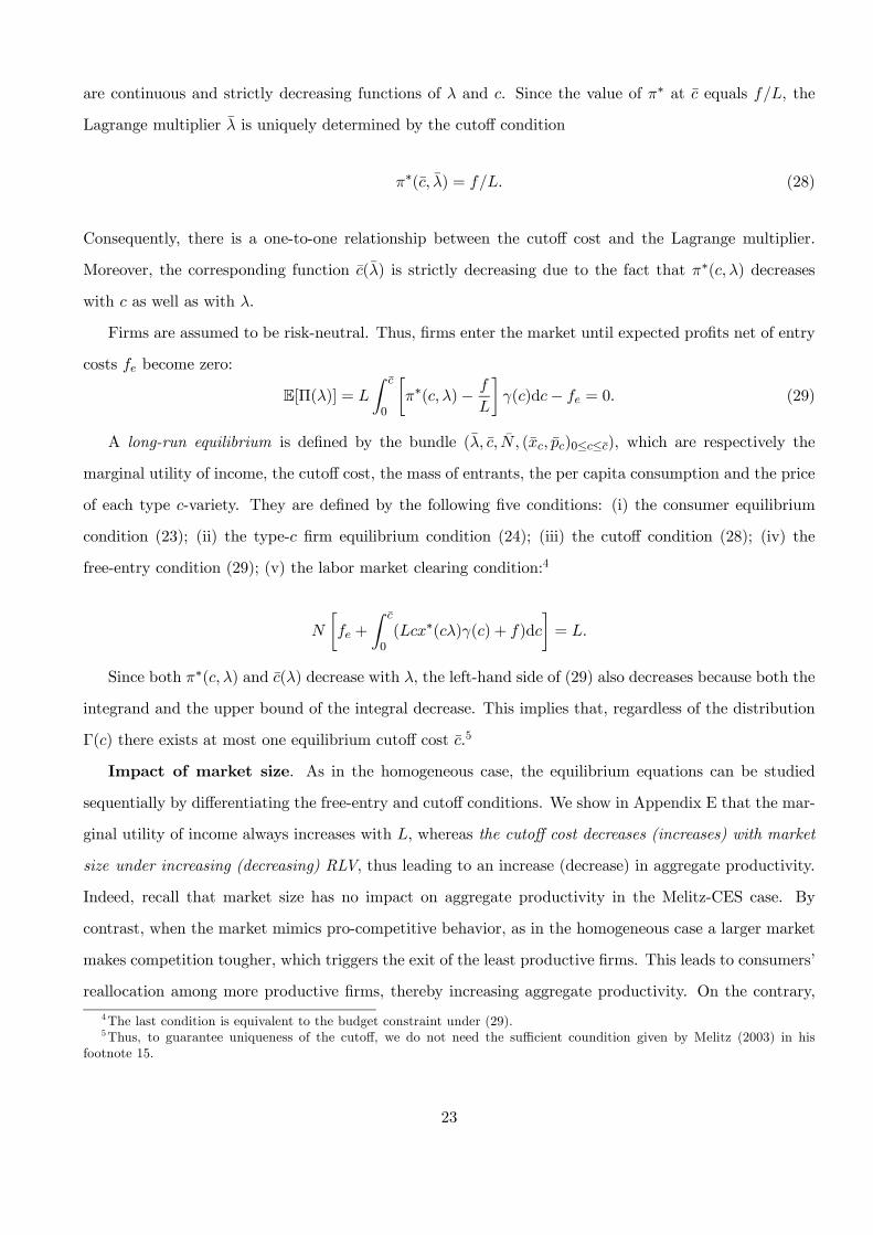
A long-run equilibrium is defined by the bundle ( ( )0≤≤), which are respectively the

marginal utility of income, the cutoff cost, the mass of entrants, the per capita consumption and the price

of each type -variety. They are defined by the following five conditions: (i) the consumer equilibrium

condition (23); (ii) the type- firm equilibrium condition (24); (iii) the cutoff condition (28); (iv) the

free-entry condition (29); (v) the labor market clearing condition:4

∙ +

Z

0

(∗()() + )d

¸=

Since both ∗( ) and () decrease with , the left-hand side of (29) also decreases because both the

integrand and the upper bound of the integral decrease. This implies that, regardless of the distribution

Γ() there exists at most one equilibrium cutoff cost .5

Impact of market size. As in the homogeneous case, the equilibrium equations can be studied

sequentially by differentiating the free-entry and cutoff conditions. We show in Appendix E that the mar-

ginal utility of income always increases with , whereas the cutoff cost decreases (increases) with market

size under increasing (decreasing) RLV, thus leading to an increase (decrease) in aggregate productivity.

Indeed, recall that market size has no impact on aggregate productivity in the Melitz-CES case. By

contrast, when the market mimics pro-competitive behavior, as in the homogeneous case a larger market

makes competition tougher, which triggers the exit of the least productive firms. This leads to consumers’

reallocation among more productive firms, thereby increasing aggregate productivity. On the contrary,

4The last condition is equivalent to the budget constraint under (29).5Thus, to guarantee uniqueness of the cutoff, we do not need the sufficient coundition given by Melitz (2003) in his

footnote 15.

23

in the price-increasing case, a larger market softens competition, which allows less productive firms to

enter, thus decreasing aggregate productivity. It is worth stressing that, as long as the cutoff exists, these

results are independent from the distribution of firms’ productivity.6

Consider now the impact of a larger market size on prices. Since () is strictly decreasing in and

strictly increasing in (see Appendix E), it follows from (25) that decreases with for all .

Therefore, (24) implies that, in the price-decreasing case, () decreases for all type- firms that remain

in business. Hence, a larger market leads to lower prices and markups because for each type- firm the

elasticity of substitution among type- varieties decreases, as in the case of homogenous firms. Moreover,

since 0 in the price-decreasing case, the average price defined by

P ≡ 1

Γ()

Z

0

dΓ()

decreases because both the integrand and the upper limit of the integral decrease. Furthermore, since

average profits are equal to Γ(), they increase with . This does not imply that all operating firms

earn higher profits in a larger economy. Indeed, using (E.2) and (E.3) in Appendix E, the elasticity of

∗( ) with respect to can be expressed as follows;

E∗() = 1− () ·R 0∗( )()dR

0∗( )()()d

where () ≡ (∗()) is increasing in in the price-decreasing case. Therefore, if is sufficiently low,

E∗() 0, meaning that these firms’ profits increase with market size. By contrast, when is close to

, we have E∗() 0 and thus the corresponding firms’ profits decrease with market size. However,

the winners gain more than the losers because average profits increase.

The opposite properties hold in the price-increasing case. In the CES case, it is readily verified that

E∗() = 0. Consequently, we have:

Proposition 6 When firms are heterogeneous in cost, the long-run equilibrium cutoff cost and prices

vary with the relative market size as follows:

6When the RLV increases, this provides an answer to Melitz web-appendix in which he questions the prediction of his

model that says that aggregate productivity does not vary with market size. To obviate this difficulty, Melitz assumes that

the elasticity of substitution among varieties is bigger when the market opens to trade than under autarky. Our approach

explains why and when this arises.

24

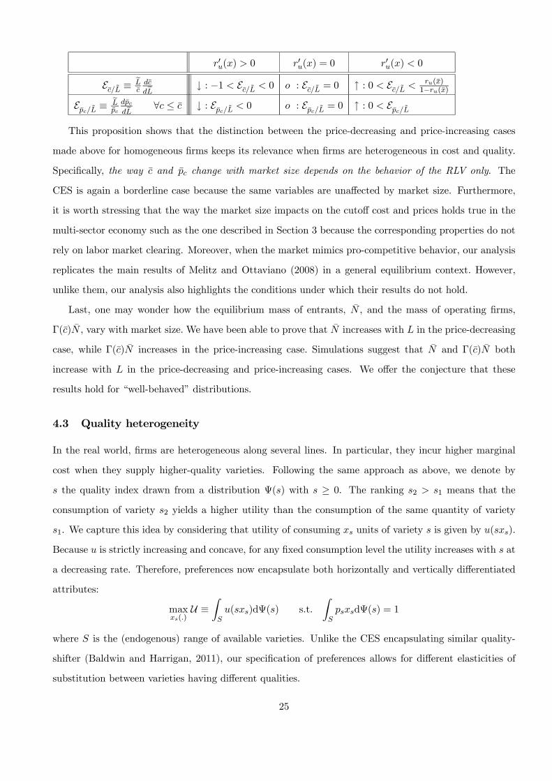
0() 0 0() = 0 0() 0

E ≡

↓ : −1 E 0 : E = 0 ↑ : 0 E ()

1−()

E ≡

∀ ≤ ↓ : E 0 : E = 0 ↑ : 0 E

This proposition shows that the distinction between the price-decreasing and price-increasing cases

made above for homogeneous firms keeps its relevance when firms are heterogeneous in cost and quality.

Specifically, the way and change with market size depends on the behavior of the RLV only. The

CES is again a borderline case because the same variables are unaffected by market size. Furthermore,

it is worth stressing that the way the market size impacts on the cutoff cost and prices holds true in the

multi-sector economy such as the one described in Section 3 because the corresponding properties do not

rely on labor market clearing. Moreover, when the market mimics pro-competitive behavior, our analysis

replicates the main results of Melitz and Ottaviano (2008) in a general equilibrium context. However,

unlike them, our analysis also highlights the conditions under which their results do not hold.

Last, one may wonder how the equilibrium mass of entrants, , and the mass of operating firms,

Γ() , vary with market size. We have been able to prove that increases with in the price-decreasing

case, while Γ() increases in the price-increasing case. Simulations suggest that and Γ() both

increase with in the price-decreasing and price-increasing cases. We offer the conjecture that these

results hold for “well-behaved” distributions.

4.3 Quality heterogeneity

In the real world, firms are heterogeneous along several lines. In particular, they incur higher marginal

cost when they supply higher-quality varieties. Following the same approach as above, we denote by

the quality index drawn from a distribution Ψ() with ≥ 0. The ranking 2 1 means that the

consumption of variety 2 yields a higher utility than the consumption of the same quantity of variety

1. We capture this idea by considering that utility of consuming units of variety is given by ().

Because is strictly increasing and concave, for any fixed consumption level the utility increases with at

a decreasing rate. Therefore, preferences now encapsulate both horizontally and vertically differentiated

attributes:

max()

U ≡Z

()dΨ() s.t.

Z

dΨ() = 1

where is the (endogenous) range of available varieties. Unlike the CES encapsulating similar quality-

shifter (Baldwin and Harrigan, 2011), our specification of preferences allows for different elasticities of

substitution between varieties having different qualities.

25

Consumers’ equilibrium conditions (23) become

() = 0()

Unlike in the above, we assume that firms know their type prior to entry. Let () be the marginal

production cost of a type -variety, which increases with the quality , with (0) = 0. The operating

profit of a firm producing a type -variety is given by

(;) =

∙0()

− ()

¸ =

∙0()

− ()

¸

Repeating the argument of Section 4.1 yields the equilibrium condition:

=()

[1− ()]=

()

1− ()∀ ∈ (30)

where

() =()

can be interpreted as the quality-adjusted marginal cost. In this case, 1() can be interpreted as the

measure of type -firms’ efficiency. In (30), () plays exactly the same role as firms’ marginal cost does

in the previous sections and thus our findings hold true where = (). By contrast, the uniqueness

of the quality cutoff requires () to be a monotone function of . Two cases may arise. First, when

() increases with , which means that () increases more than proportionally with quality , the

quality-adjusted cost and the quality rankings are the same, then only the firms offering a quality smaller

than or equal to the cut off are in business ( = [0 ]). In other words, when () is strictly convex,

the high-quality varieties have too high prices for the corresponding firms to survive. Second, when ()

increases less than proportionally with quality , only the varieties whose quality exceeds are available

( = [∞)). Stated differently, when () is strictly concave, the low-quality firms are unable to price

their variety at a sufficiently low price to break even. When () is neither convex nor concave, there can

be more than one quality cutoff. For example, when () is inverted U-shaped, only high- and low-quality

varieties are available.

Firms’ pricing rules now depend on the interaction between the RLV and the quality-adjusted cost.

Indeed, high quality goods may be associated with higher or lower markups depending on the assumptions

made on and (). Specifically, we readily verify that the following results hold.

26

Proposition 7 When firms are heterogeneous in cost and quality, we have:

0() 0 0() = 0 0() 0

0() 0 ↓ () ↓ : E() 0 : E() = 0 ↑ () ↑ : E() 0

⇒ = [0 ] ↓ : E 0 ↓ : E 0 : E = E = 0 ↑ : E 0 ↑ : E 0

0() 0 ↑ () ↓ : E() 0 : E() = 0 ↓ : () ↑ : E() 0

⇒ = [+∞) ↑ : E 0 ↓ : E 0 : E = E = 0 ↓ : E 0 ↑ : E 0

In words, when () is strictly convex (concave), firms with higher (lower) quality charge lower

(higher) markups in the price-decreasing case, but higher (lower) markups when the market mimics anti-

competitive behavior. Moreover, the cutoff quality decreases (increases) with market size in the price-

decreasing (price-increasing) case because tougher (softer) competition drives high-quality varieties out

of business (invites low-quality varieties). The average efficiency corrected for quality does not depend

on the concavity/convexity of (). It always increases in the price-decreasing case, and decreases in

the price-increasing one. Last, observe that the impact of market size on markups is the same as in

the homogeneous case. In other words, the market selects the qualities with the best quality-adjusted

marginal costs and eliminates the others, very much as in oligopolistic models of vertical differentiation

(Shaked and Sutton, 1983).

Among other things, the above proposition does not support the widely spread idea that developed

countries should necessarily aim to produce high-quality products to insulate their workers from compet-

ition with emerging countries. Our results show that a high quality is not sufficient to endow firms with

a strong competitive advantage. What matters for them to survive on the international marketplace is

the level of their quality-adjusted cost within the product range.

5 Non-additive preferences

It is natural to ask whether our approach may comply with non-additive preferences. In what follows,

we consider the quadratic utility in the homogeneous case (Ottaviano et al., 2002; Melitz and Ottaviano,

2008). The utility of variety is given by

(X) = −

22 − X (31)

27

where is a positive parameter measuring the substitutability between variety and any other variety ,

while

X ≡Z

0

d

denotes the total consumption of the differentiated product. The assumption of non-additive preferences

is reflected by the fact that the utility derived from consuming variety is shifted downward according

to the total consumption of the differentiated good. Moreover, the RLV is also shifted downward when

varieties become more differentiated. In this event, consumers display a weaker love for variety. To ease

the burden of notation, we set = 1.

Applying the first-order conditions for utility maximization yield the individual inverse demand func-

tions:

(X) =1− −X

where is again the marginal utility of income. Compared to (4), the inverse demand for a variety now

depends on two aggregate statistics, that is, and X. The latter aggregate statistic accounts for variety

demand linkages that are not taken into account by general additive preferences.

Since the impact of on X is negligible, we have

=

1− −X

which increases with . This suggests that quadratic preferences generate pro-competitive behaviors. To

check it, consider a symmetric outcome with = and X =. In this event, the market price must

solve the following quadratic equation:

= +

− ( +)

which has two real roots. The larger root exceeds whereas the other is smaller than . Therefore, the

short-run equilibrium price is unique and given by

1() =(1 + ) + 2 +

p(1− )22 + 4 + 42

2

Differentiating this expression with respect to shows that the market price decreases with . It remains

to determine the equilibrium mass of firms in the long run. It follows from (17) that () = . Since

() decreases with , it must that increases with . As a result, a one-sector economy in which

28

consumers are endowed with quadratic preferences behaves like a pro-competitive economy such as those

described in Section 2.

Alternately, the equilibrium price 1() can be obtained by using the following extension of additive

preferences in which the subutility now depends on the mass of available varieties:

U ≡Z

0

( )d (32)

where

() ≡ 1− [1− ( +)]2++

is strictly increasing and concave in over [0 1( +)). Using (32), we can repeat mutatis mutandis

the arguments of Sections 2.2. and derive 1() as in Proposition 1. This suggests that preferences (32)

can be used to cope with interactions across varieties similar to those encapsulated in the quadratic utility

(31).7

The foregoing discussion is reminiscent of what we know from the two-sector model of Section 3 when

(31) is nested into a quasi-linear upper-tier utility. In this case, there is no income effect, thereby implying

that = 1. The inverse demand then becomes

( ) = 1− −X

so that

2() =

2 ++

+

2 +

which also decreases with since must be smaller than 1 for consumers to purchase the differentiated

product (Ottaviano et al., 2002). Note that 1() 2(), the reason being that firms producing the

differentiated good compete with the producers of the homogeneous good in the two-sector setting.

Since the analysis above also applies to the translog utility studied by Feenstra (2003), we may conclude

that the assumption of additive preferences is not be as restrictive as it looks like at first glance.

6 Concluding remarks

Our purpose was to develop a general, but tractable, model of monopolistic competition which obviates the

shortcoming of the CES discussed in the introduction. This new model encompasses features of oligopoly

7Another example of (32) is provided by Benassy (1996) where () = , being a constant that exceeds

−1( − 1).

29

theory, while retaining most of the flexibility of the CES model of monopolistic competition. Thus, we

find it fair to say that our model builds a link between the two main approaches to imperfect competition.

Moreover, without having the explicit solution for the equilibrium outcome, we have been able to provide

a full characterization of the market equilibrium and to derive necessary and sufficient conditions for

the market to mimic price-decreasing and price-increasing behaviors under well-behaved utility functions.

That the market outcome is characterized through necessary and sufficient conditions on preferences

implies that it becomes possible to check the full economic consistency between assumptions made in

empirical models and the results obtained after estimation. More importantly, perhaps, our analysis

shows that relatively minor changes in the specification of utility may result in opposite predictions, thus

highlighting the need to be careful in the use of specific functional forms.

We would be the last to claim that using the CES is a defective research strategy. Valuable theoretical

insights may be derived from this model by taking advantage of its various specificities. However, having

shown how peculiar are the results obtained under a CES utility, it is our contention that a “theory”

cannot be built on this model. Things are more problematic for empirical studies. Indeed, the CES being

a borderline case, using this framework is unlikely to permit (quasi-) structural estimations. The use of

alternative and richer specifications of preferences therefore should rank high on the research agenda of

both theorists and empirical economists.

Given the huge number of applications of the CES, it seems natural to ask whether our results should

lead CES-users to revisit their analysis. A fairly wide range of results is likely to hold regardless of

the behavior of the RLV. However, it is not easy to predict which results are CES-specific and how

they will be affected. In an early version of this paper, we have studied firms’ pricing in a model à la

Krugman with iceberg trade costs. In such a context, one of the most problematic results obtained under

the CES is that the pass-on just equals trade costs. Zhelobodko et al. (2010) show that firms’ pricing

involves dumping (reverse dumping) when the RLV is increasing (decreasing). Moreover, firms belonging

to different countries need not adopt the same pricing policies. This is sufficient to illustrate how our

modeling strategy can be used to understand why and how firms choose their pricing policies (Manova

and Zhang, 2009; Martin, 2009). Clearly, more work is called for.

References

[1] Amir, R. and V.L. Lambson (2000) On the effects of entry in Cournot markets. Review of Economic

Studies 67, 235-254.

30

[2] Baldwin, R. and J. Harrigan, J. (2011) Zeros, quality and space: trade theory and trade evidence.

The American Economic Journal: Microeconomics, forthcoming.

[3] Behrens, K and Y. Murata (2007) General equilibrium models of monopolistic competition: a new

approach. Journal of Economic Theory 136, 776-787.

[4] Bénassy, J.-P. (1996) Taste for variety and optimum production patterns in monopolistic competition.

Economics Letters 52, 41—47.

[5] Bertoletti, P.E. Fumagalli and C. Poletti (2008) On price-increasing monopolistic competition. Memo,

Università di Pavia.

[6] Bernard, A.B., J. Eaton, J.B. Jensen, and S. Kortum (2003) Plants and productivity in international

trade. American Economic Review 93, 1268-1290.

[7] Badinger, H. (2007) Has the EU’s Single Market Programme fostered competition? Testing for a

decrease in mark-up ratios in EU industries. Oxford Bulletin of Economics and Statistics 69, 497-519.

[8] Broda, C. and D.E. Weinstein (2006) Globalization and the gains from variety. Quarterly Journal of

Economics 121, 541-585.

[9] Campbell, J.R. and H.A. Hopenhayn (2005) Market size matters. Journal of Industrial Economics

LIII, 1-25.

[10] Chen, Y. and M.H. Riordan (2007) Price and variety in the spokes model. Economic Journal 117,

897-921.

[11] Chen, Y. and M.H. Riordan (2008) Price-increasing competition. Rand Journal of Economics 39,

1042-1058.

[12] Dixit, A.K. and V. Norman (1980) Theory of International Trade. Cambridge: Cambridge University

Press.

[13] Dixit, A.K. and J.E. Stiglitz (1977) Monopolistic competition and optimum product diversity. Amer-

ican Economic Review 67, 297-308.

[14] Feenstra, R.C. (2003) A homothetic utility function for monopolistic competition models, without

constant price elasticity. Economics Letters 78, 79-86.

31

[15] Head, K. and T. Mayer (2004) The empirics of agglomeration and trade. In Handbook of Regional

and Urban Economics, Volume 4 (ed. J. V. Henderson and J.-F. Thisse), 2609—69. Amsterdam:

North-Holland.

[16] Head, K. and J. Ries (2001) Increasing returns versus national product differentiation as an explan-

ation for the pattern of US-Canada trade. American Economic Review 91, 858-876.

[17] Holmes, T.J. and J.J. Stevens (2004) Geographic concentration and establishment size: analysis in

alternative economic geography models. Journal of Economic Geography 4, 227-250.

[18] Holmes, T.J. and J.J. Stevens (2010) Exports, border, distance, and plant size. NBERWorking Paper

16046.

[19] Houthakker, H.S. (1960) Additive preferences. Econometrica 28, 244-257.

[20] Krugman, P.R. (1979) Increasing returns, monopolistic competition, and international trade. Journal

of International Economics 9, 469-479.

[21] Krugman, P.R. (1980) Scale economies, product differentiation, and the pattern of trade. American

Economic Review 70, 950-959.

[22] Manning, A. (2010) Agglomeration and monoposony power in labour markets. Journal of Economic

Geography 10717-744.

[23] Manova, K. and Z. Zhang (2009) Quality heterogeneity across firms and export destinations. NBER

Working Paper No. 15342.

[24] Martin, J. (2009) Spatial price discrimination in international markets. CEPII Working Paper

N◦2009-21.

[25] Melitz, M.J. (2003) The impact of trade on intraindustry reallocations and aggregate industry pro-

ductivity. Econometrica 71, 1695-1725.

[26] Melitz, M.J. and G.I.P. Ottaviano (2008) Market size, trade, and productivity. Review of Economic

Studies 75, 295-316.

[27] Nadiri, M.I. (1982) Producers theory. In Arrow, K.J. and M.D. Intriligator (eds.) Handbook of Math-

ematical Economics. Volume II. Amsterdam: North-Holland, pp. 431-490.

32

[28] Neary, J.P. (2004) Monopolistic competition and international trade theory. In Brakman, S. and

B.J. Heijdra (eds.) The Monopolistic Competition Revolution in Retrospect. Cambridge: Cambridge

University Press, pp. 159-184.

[29] Ottaviano, G.I.P., T. Tabuchi, and J.-F. Thisse (2002) Agglomeration and trade revisited. Interna-

tional Economic Review 43, 409-436.

[30] Shaked, A. and J. Sutton (1983) Natural oligopolies. Econometrica 51, 1469-1483.

[31] Spence, M. (1976) Product selection, fixed costs, and monopolistic competition. Review of Economic

Studies 43, 217-235.

[32] Syverson, C. (2007) Prices, spatial competition, and heterogeneous producers: an empirical test.

Journal of Industrial Economics LV, 197-222.

[33] Vives, X. (1999) Oligopoly Pricing. Old Ideas and New Tools. Cambridge, MA: The MIT Press.

[34] Ward, M.B., J.P. Shimshack, J.M. Perloff, and J.M. Harris (2002) Effects of the private-label invasion

in food industries. American Journal of Agricultural Economics 84, 961-973.

[35] Zhelobodko, E., S. Kokovin and J.-F. Thisse (2010) Monopolistic competition: beyond the CES.

CEPR Discussion Paper No.7947.

Appendix

A. Existence and uniqueness of a short-run equilibrium

Existence. Set ≡ 1. The function () ≡ 1− − () is negative at = 1 and positive at

= 0 by (9). Therefore, since () is continuous, () = 0 has at least one positive solution.

Uniqueness. We show that 0() = − − 0 () is negative at any solution to () = 0.

Multiplying 0() by and using the condition () = 0, we get

0() = ()− 1− 0 ()

Since

0 ≡ (1 + − 0)

holds for all , it follows from (8) that

33

1− + 0 = 1 + 2 − 0 (1− )2 ≥ 0 (A.1)

Evaluating (A.1) at = , we obtain 0() 0 at any solution to () = 0, which implies that the

solution is unique.

B. The impact of market size and cost on consumption and production

Consumption. Differentiating (15) and using (19), we get the elasticity

E ≡

=

= E = −1−

1

1− E 0

Since E − 1, we have E −1. The equilibrium consumption of each variety thus decreases

with and with regardless of the sign of 0. These effects are similar to those obtained under the CES.

Production. Recall that a firm’s production is given by = . Thus, the elasticities of with

respect to and are the same. Note that the sign is a priori undetermined because decreases with .

However, since

E ≡

= 1 + E = −

1

1− E

and since E = E, it must be that and have opposite signs.

The impact of marginal cost. When the marginal cost increases, everything else being equal,

operating profits are lower so that the economy accommodates fewer firms. However, when 0 0, a

smaller mass of firms leads to a higher market price. Therefore, the impact of an increase in generates

two opposite effects. In order to determine the global impact, we rewrite the equilibrium markup as

follows

() =

1− ()

Using (19), this implies

E ≡

= 1 +

1−

1− 0

Consequently, the market price always increases with the marginal cost, regardless of the sign of 0.

However, the elasticity of with respect to depends on the sign of 0. Indeed, if 0 0, we have

0. In this case, the above expression implies that 1 ()() 1 − . Thus, each

firm absorbs some fraction of the cost increase. On the other hand, if 0 0, we have ()() 1,

meaning that a higher marginal cost leads to a more than proportional increase in market price.

34

To determine the impact of on the mass of firms, we differentiate () = () with respect to

, use (20), and get

E ≡

=

= E = E

Thus, when rises, the equilibrium mass of firms may go up or down. Specifically, when 0 0, the

equilibrium price decreases with , which together with (19) imply

−(1− ) E 0

whereas we have E 0 when 0 0. Note that, for 0 = 0, an increase or a decrease in the marginal

cost has no impact on the equilibrium mass of firms.

C. Properties of the expenditure function in the two-sector economy

The following two lemmas allow one to rationalize the assumption (22) made in Proposition 4.

Set

≡ 0011 ·¡0¢2 − 2 00120 + 0022 + 01

00

Lemma 1 If 0021 ≥ 0, then the elasticity of w.r.t. is such that

· − 1 = −

0011

0 + 0021 ( + 0)− 0022

≤ 0

Recall that = 0 denotes the elasticity of the lower-tier utility .

Lemma 2 If 0021 ≥ 0 and the inequality

1− ()

()≤ 0021( )

02( )− 0011( )

01( )(C.1)

hold at a symmetric outcome, then the elasticity of w.r.t. is such that

−1 ≤

· − 1 = 01

0 + 0021

0 − 0022

≤ 0 (C.2)

Remark 1. In the special case of a Cobb-Douglas upper utility, the right-hand side of (C.1) is 1 so

that this condition boils down to

1 ≤ () + ()

35

which holds for many functions , including the CES where () = 1− and () = .

Remark 2. Under (0) = 0, the indirect utility function

() =

µ

¶

is homogeneous of degree 0 w.r.t. () and of degree 1 w.r.t. (). Therefore, 0 and 0 are

homogeneous of degree −1 w.r.t. () and of degree 0 w.r.t. (). Finally, we have 00 0.

Before proceeding, recall that the first-order condition for the upper-tier utility maximization (21) is

given by

01(() 1−)0()− 02(() 1−) = 0 (C.3)

while the second-order condition is given by

0

Note that (( ) 1−) is concave w.r.t. because is concave while the concavity of implies

that of .

Proof of Lemma 1. Differentiating (C.3) w.r.t. and solving for , we get

= −

0011

0

0 + 01

00 − 0021

0

= −(

0011

0 − 0021)

0 + 01

00

Consequently,

· − 1 = − (

0011

0 − 0021)

0 + 01

00

− 1 =

− 0011h00 + (0)

2i+ 0021 (0 + 2

0)− 01 (00 +00)− 0022

Applying the Euler theorem to and 0, we obtain the following equalities:

− 0011h00 +

¡0¢2i

= − 00110¡0 +0

¢= − 00110

0021¡0 + 2

0

¢= 0021

¡ +0

¢− 01

¡00 +00

¢= 0

As a result, we have:

· − 1 = −

0011

0 + 0021 ( +0)− 0022

36

Since 0021 ≥ 0, the numerator of this expression is positive. Since 0, we have

· − 1 ≤ 0

Proof of Lemma 2. Differentiating (C.3) w.r.t. and solving for , we get

=− 001100 − 01

00 + 0021

0

(C.4)

which implies

· − 1 =

− 001100 − 0100 + 0021

0

− 1

=− 0011

h00 + (0)

2i− 01

³00 +00

´+ 0021

¡0 + 20

¢− 0022

Applying the Euler theorem to and 0 yields

− 0011h0

0 +

¡0¢2i

= − 00110¡0 +0

¢= 0

and

− 01¡00 +00

¢= 01

0 0

Therefore,

· − 1 = 01

0 + 0021

0 − 0022

≤ 0

since 0021 ≥ 0 Consequently, the right inequality of (C.2) is proven.To show that 0, we rewrite (C.4) as follows:

=

0

Ã− 00110 − 01

000

+ 0021

! (C.5)

By definition of , we have

0 = −0

2 0 0 =

0

00 = −

0

2− 00

3

Since 0 0, the sign of is the same as that of the bracketed term of (C.5). Substituting these

37

three expressions into (C.5) leads to

− 00110 − 01000

+ 0021

= − 00110

− 01

− 02− 00

3

−02

+ 0021

= −01

∙µ 0011

01− 0021

02

¶0

+ 1 +

00

0

¸

Using − 01 0 and 010() = 02

0, it follows from (C.1) that

µ 0011

01− 0021

02

¶0

+ 1 +

00

0 0 =⇒

0

which implies the left inequality of (C.2).

D. The impact of market size on the mass of firms in the two-sector economy

We show that the equilibrium mass of firms decreases with the market size (see Proposition 5). To this

end, we exploit the following implicit relationship between and :

= ()(() )

Differentiating this expression w.r.t. , we get

· = 1 +

+

+

which implies

·

µ1−

¶= 1 +

µ1 +

1−

¶

Using (22), we obtain

·

µ1−

¶≥ 1 +

µ1 +

1−

¶( − 1)

=

µ1−

¶ 0

which implies

·

0

38

E. The impact of market size when firms are heterogeneous

Let E∗ and E∗ be the elasticities of ∗( ) w.r.t. and , respectively. Differentiating (27) and

using the envelope theorem, we obtain

∗( )

= −∗()

Hence, we have

E∗ =−∗()

[∗( )− ]∗()=

−

1−(∗()) − = 1− (∗()) ≡ 1− () 0 (E.1)

Furthermore, applying the envelop theorem to

∗( ) =∙0(∗())

−

¸∗()

yields

∗( )

= −0(∗())

2∗()

which leads to

E∗ = −1

(∗())= −(∗()) ≡ −() 0 (E.2)

Impact of market size on the marginal utility of income. To see how the marginal utility

of income changes with , we divide the free-entry condition (29) by and differentiate the resulting

expression w.r.t. :

Z

0

∗( )

()d+

∙∗( )−

¸

= −Γ()

2−

2= −

R 0∗( )()d

0

where ∗( )− = 0 so that the derivative of can be neglected. Rewriting this expression in terms

of elasticities and using (E.2), the elasticity E can be rewritten as follows:

E = −R 0∗( )()dR

0∗()

()d

= −R 0∗( )()dR

0∗( )E∗()d

=

R 0∗( )()dR

0∗( )()()d

(E.3)

which takes on values between 0 and 1.

Impact of market size on the cutoff cost. Differentiating the cutoff condition (28) w.r.t. :

39

∗( ) =

∗( )

+

∗( )

= −

2

Rewriting this expression in terms of elasticities and using (E.1) and (E.2), we obtain

∗( )

[1− ()]−

∗( )

() = −

2= −

∗( )

Denoting the elasticity of the cutoff cost w.r.t. as E, we get:

E · [1− ()]− E() = −1

and thus

E =1− E()()− 1

Plugging (E.3), we obtain:

E =1− ()

0∗()()d

0∗()()()d

()− 1 (E.4)

Since the denominator of this expression is positive, the sign of elasticity is positive if and only the second

term of the numerator is smaller than 1. In the price-decreasing case, we know that () decreases.

Therefore, () () for all because ∗() is decreasing. The second term of the numerator is

then larger than 1, and E 0. Similarly, E 0 in the price-increasing case, while E = 0 in theCES.

Furthermore, we have the following bounds on E:

−1 E 1

()− 1

It follows from (E.4) that

E · [()− 1]− 1 0

It remains to show that E is bigger than −1, i.e. E + 1 0. Indeed, adding 1 on both sides of (E.4)and rearranging terms yields

()

"1−

R 0∗( )()dR

0∗( )()()d

#(()− 1) 0

because 1.

40