Monographs in Mathematics Vol. 89

Managing Editors: H.Amann UniversiHit Zurich, Switzerland K. Grove University of Maryland, College Park H. Kraft UniversiUit Basel, Switzerland P.-L. Lions Universite de Paris-Dauphine, France

Associate Editors: H. Araki, Kyoto University J. Ball, Heriot-Watt University, Edinburgh E Brezzi, Universita di Pavia K.C. Chang, Peking University N. Hitchin, University of Warwick H. Hofer, Universitat Bochum H. Knorrer, ETH Zurich K. Masuda, University of Tokyo D. Zagier, Max-Planck-Institut Bonn

Herbert Amann

Linear and Quasilinear PamboHc Problems Volume I Abstract Linear Theory

1995 Birkhauser Verlag Basel· Boston· Berlin

Author: Institut fUr Mathematik Universitat Ziirich Winterthurerstrasse 190 8057 Ziirich Switzerland

A CIP catalogue record for this book is available from the Library of Congress, Washington D.C., USA

Die Deutsche Bibliothek - CIP-Einheitsaufnahme Amann, Herbert: Linear and quasilinear parabolic problems I Herbert Amann. -Basel; Boston; Berlin: Birkhauser Vol. 1. Abstract linear theory. - 1995 (Monographs in mathematics; Vol. 89)

ISBN-13: 978-3-0348-9950-5 e-ISBN-13: 978-3-0348-9221-6 DOl: 978-3-0348-9221-6

This work is subject to copyright. All rights are reserved, whether the whole or part of the material is concerned, specifically the rights of translation, reprinting, re-use of illustrations, broadcasting, reproduction on microfilms or in other ways, and storage in data banks. For any kind of use permis­sion of the copyright owner must be obtained.

© 1995 Birkhauser Verlag Basel, P.O. Box 133, CH-4010 Basel, Switzerland Printed on acid-free paper produced of chlorine-free pulp

Softcover reprint of the hardcover I st edition 1995

987654321

Aber - so fragen wir - wird es bei der Ausdehnung des mathematischen Wissens fUr den einzelnen Forscher nicht schliel3lich unmoglich, alle Teile dieses Wissens zu umfassen? Ich mochte als Antwort darauf hinweisen, wie sehr es im Wesen der mathematischen Wissenschaft liegt, daB jeder wirkliche Fortschritt stets Hand in Hand geht mit der Auffindung scharferer Hilfsmittel und einfacherer Methoden, die zugleich das Verstandnis friiherer Theorien erleichtern und umstandliche altere Entwicklungen bcseitigen, und daB es daher dem einzelnen Forscher, indem er sich diese scharferen Hilfsmittel und einfacheren Methoden zu eigen macht, leichter gelingt, sich in den verschiedenen Wissenszweigen der Mathematik zu orientieren, als dies fUr irgend eine andere Wissenschaft der Fall ist. 1

David Hilbert {1862-1943}

1 But - so we ask - given tne expansion of mathematical knowledge, will it eventually not be impossible for the individual researcher to encompass all parts of this knowledge? As an answer I want to point out how much it lies in the character of mathematical science that all real progress is intimately tied to the discovery of sharper tools and simpler methods that, at the same time, facilitate the comprehension of earlier theories and remove complicated older developments, and that therefore the researcher, adopting these sharper tools and simpler methods, succeeds in getting more easily acquainted with the diverse branches of mathematics than this is the case for any other field of science.

Preface

In this treatise we present the semigroup approach to quasilinear evolution equa­tions of parabolic type that has been developed over the last ten years, approxi­mately. It emphasizes the dynamic viewpoint and is sufficiently general and flexible to encompass a great variety of concrete systems of partial differential equations occurring in science, some of those being of rather 'nonstandard' type. In partic­ular, to date it is the only general method that applies to noncoercive systems.

Although we are interested in nonlinear problems, our method is based on the theory of linear holomorphic semigroups. This distinguishes it from the theory of nonlinear contraction semigroups whose basis is a nonlinear version of the Hille­Yosida theorem: the Crandall-Liggett theorem. The latter theory is well-known and well-documented in the literature. Even though it is a powerful technique having found many applications, it is limited in its scope by the fact that, in concrete applications, it is closely tied to the maximum principle. Thus the theory of nonlinear contraction semigroups does not apply to systems, in general, since they do not allow for a maximum principle. For these reasons we do not include that theory.

Our approach is strongly motivated by the concept of weak solutions of dif­ferential equations. In fact, as one of the applications of our general results we cventually develop a theory of weak solutions for noncoercive quasilinear parabolic systems in divergence form in an Lp-setting. This is in contrast to the standard L2-setting for coercive problems, that is, unfortunately, not suitable for noncoer­cive systems. Moreover, even in regular situations, where, in principle, we could work directly within the framework of strong solutions, the theory of weak so­lutions is of great importance. For instance, in connection with global existence it allows for a priori estimates in 'weak norms', which facilitates the establish­ing of those bounds considerably. For this reason we develop a general 'reflexive' theory taylored for applications in an Lp-setting. We treat evolution equations in spaces of continuous functions only marginally. An exposition of the latter theory, emphasizing fully nonlinear problems and strong solutions, can be found in the monograph by A. Lunardi [LungS].

In order to obtain results that are sufficiently general and flexible to be ap­plicable to a wide variety of concrete problems, we need a considerable amount of

viii Preface

preparation. For this reason our treatise is divided in three volumes, carrying the respective titles:

Abstract Linear Theory,

Function Spaces and Linear Differential Operators,

Nonlinear Problems.

In the first volume we give a thorough discussion of linear parabolic evolution equations in general Banach spaces. This is the abstract basis for the nonlinear theory. The second volume is devoted to concrete realizations of linear parabolic evolution equations by general parabolic systems. There we discuss the various function spaces that are needed and useful, and the generation of analytic semi­groups by general elliptic boundary value problems. The last volume contains the abstract nonlinear theory as well as various applications to concrete systems, il­lustrating the scope and the flexibility of the general results. Of course, each one of the three volumes contains much material of independent interest related to our main subject.

In writing this book I had help from many friends, collegues, and students. It is a pleasure to thank all of them, named or unnamed. I am particularly indebted to P. Quittner and G. Simonett, who critically and very carefully read, not only the whole manuscript of this first volume but also many earlier versions that were produced over the years and will never be published, and pointed out numerous mistakes and improvements. Large parts of the first volume, and of earlier versions as well, were also read and commented on by D. Daners, J. Escher, and P. Guidotti. Their constructive criticism, observations, and suggestions for improvements were enormously helpful. Of course, I am solely responsible for all remaining mistakes.

My son Andreas gave expert advice for taming the computer and kept open an emergency line. Finally, this book would never have appeared without the invaluable help of my 'comma sniffer', whose contributions are visible on every page. My heartfelt thanks go to both of them.

Through many years I obtained financial support by Schweizerischer N a­tionalfonds, that is gratefully acknowledged. It enabled me to maintain an active group in this field of research and to bring in visitors from outside. These contacts were enormously beneficial for my work. I also express my gratitude to Birkhauser Verlag, in particular to Th. Hintermann, for the agreeable collaboration.

Zurich, December 1994 Herbert Amann

Contents

Preface . ...

Introduction

1 2 3 4 5

Notations and Conventions

Topological Spaces . . . Locally Convex Spaces ... . Complexifications ..... . Unbounded Linear Operators General Conventions . . . . .

Chapter I Generators and Interpolation

1 Generators of Analytic Semigroups

1.1 Properties of Linear Operators 1.2 The Class H(Ell Eo) .. 1.3 Perturbation Theorems 1.4 Spectral Estimates ... 1.5 Compact Perturbations 1.6 Matrix Generators . . .

2 Interpolation FUnctors

2.1 Definitions ....... . 2.2 Interpolation Inequalities 2.3 Retractions ....... . 2.4 Standard Interpolation Functors 2.5 Continuous Injections 2.6 Duality Properties . . 2.7 Compactness..... 2.8 Reiteration Theorems 2.9 Fractional Powers and Interpolation 2.10 Semigroups and Interpolation ... 2.11 Admissible Interpolation Functors .

vii

xiii

1 2 4 6 7

10 11 14 15 20 21

24 25 26 28 30 30 31 31 32 33 35

x Contents

Chapter II Cauchy Problems and Evolution Operators

1 Linear Cauchy Problems

1.1 1.2

Holder Spaces ....... . Existence and Regularity Theorems

2 Parabolic Evolution Operators

2.1 2.2

3

3.1 3.2 3.3

4

4.1 4.2 4.3

4.4 4.5

Basic Properties . . . . . . . . . Determining Integral Equations. . .

Linear Volterra Integral Equations

Weakly Singular Kernels. . . . Resolvent Kernels . . . . . . . Singular Gronwall Inequalities

Existence of Evolution Operators

A Class of Parameter Integrals . . . . Semigroup Estimates ........ . Construction of Evolution Operators . The Main Result . . . . . . . . . . Solvability of the Cauchy Problem

5 Stability Estimates

5.1 5.2 5.3 5.4

Estimates for Evolution Operators Continuity Properties of Mild Solutions Holder Estimates . . . . . . . . Boundedness of Mild Solutions

6 Invariance and Positivity

6.1 6.2 6.3 6.4

Yosida Approximations ........ . Approximations of Evolution Operators Invariance. . . . . . . . . Orderings and Positivity. . . . . . . .

Chapter III Maximal Regularity

1

1.1 1.2 1.3 1.4 1.5 1.6

General Principles

Sobolev Spaces .......... . Absolutely Continuous Functions . Generalized Solutions . . . . Trace Spaces ........ . Pairs of Maximal Regularity Stability ........... .

40 43

45 47

48 50 52

53 55 57 63 66

68 71 72 74

75 77 80 84

88 89 91 92 94 96

Contents

2 Maximal HOlder Regularity

2.1 2.2 2.3 2.4 2.5 2.6

Singular HOlder Spaces Semigroup Estimates 'frace Spaces . . . . Estimates for K A . . .

Maximal Regularity Nonautonomous Problems.

3 Maximal Continuous RegUlarity

3.1 3.2 3.3 3.4

Necessary Conditions ...... . Higher Order Interpolation Spaces Estimates for K A . .

Maximal Regularity . . . . . . .

4 Maximal Sobolev Regularity

4.1 Temperate Distributions . . . . . 4.2 Fourier 'fransforms and Convolutions 4.3 The Hilbert 'fransform ........ . 4.4 UMD Spaces and Fourier Multipliers. 4.5 Properties of UMD Spaces 4.6 Fractional Powers ..... 4.7 Bounded Imaginary Powers 4.8 Perturbation Theorems . . 4.9 Sums of Closed Operators . 4.10 Maximal Regularity ....

Chapter IV Variable Domains

1 Higher Regularity

1.1 1.2 1.3 1.4 1.5

Properties of Differentiable Functions . . . . . . General Solvability Results for Cauchy Problems Estimates for Evolution Operators . . . . . . Evolution Operators on Interpolation Spaces The Cauchy Problem ............ .

2 Constant Interpolation Spaces

2.1 2.2 2.3 2.4 2.5 2.6

Semigroup and Convergence Estimates. Assumptions and Consequences. . . . Construction of Evolution Operators . Estimates for Evolution Operators . The Cauchy Problem ....... . Abstract Boundary Value Problems

xi

98 102 106 109 113 117

121 123 124 126

128 130 135 141 144 147 162 168 173 180

194 195 198 204 207

211 214 218 227 230 233

xii Contents

3 Maximal Regularity

3.1 3.2

Abstract Initial Boundary Value Problems Isomorphism Theorems . . . . . . . . . . .

Chapter V Scales of Banach Spaces

1 Banach Scales

1.1 1.2 1.3 1.4 1.5

General Concepts Power Scales . . . Extrapolation Spaces Dual Scales . . . . . . Interpolation-Extrapolation Scales

2 Evolution Equations in Banach Scales

2.1 2.2 2.3 2.4 2.5 2.6 2.7 2.8

Semigroups in Interpolation-Extrapolation Scales. Parabolic Evolution Equations in Banach Scales Duality ......... . Approximation Theorems . . Final Value Problems . . . . Weak Solutions and Duality. Positivity . . . . . . . . . . . General Evolution Equations

Bibliography . .

List of Symbols

Index ...... .

242 245

250 255 261 267 275

286 294 297 300 304 307 312 314

321

329

333

Introduction

Nichts setzt clem Fortgang cler Wis­senschaft mehr Hinclernis entgegen als wenn man zu wissen glaubt, was man noch nicht weiB.l

Georg Christoph Lichtenberg (1742-1799)

Partial differential equations of parabolic type are encountered in a variety of problems in mathematics, physics, chemistry, biology, and many other scientific subjects in which irreversible processes can be adequately described by mathemat­ical models. For this reason parabolic equations have been thoroughly studied and there is a considerable mathematical literature in this field. However, most of the research has been concentrated on the study of a single second order parabolic equation for one scalar-valued unknown - at least as far as nonlinear equations are concerned - and on certain particular systems for a vector-valued unknown describing specific physical situations. The Navier-Stokes equations of hydrody­namics are among the most eminent representatives of the latter class.

During the last two or three decades, so-called reaction-diffusion equations have become a much favored object of study by application-oriented analysts. In contrast to the classical investigations in the theory of partial differential equations, that concentrate on questions of existence and uniqueness, there has been devel­oped a more qualitative, dynamical-systems-type approach to reaction-diffusion equations. The basic idea of this method is to interprete the partial differential equation as an ordinary differential equation in an infinite-dimensional Banach space. This assigns a predominant role to the time variable and relegates the spa­cial dependence to the set-up, that is, to the correct choice of the underlying function spaces and to the properties of the operators representing the partial differential equations. Having found the right frame for this description one can try to mimic the finite-dimensional theory of ordinary differential equations to ob­tain information on the long-time behavior of solutions, their stability properties, bifurcation phenomena, etc., questions of paramount interest in applications.

The ordinary-differential-equations-approach to time-dependent partial dif­ferential equations has proven to be very powerful. It is by no means restricted to simple semilinear reaction-diffusion equations as they are studied in the litera­ture most often. In fact, it is one of the main purposes of this treatise to extend this approach to general quasilinear parabolic systems encompassing a great vari­ety of concrete equations from science. In addition, by our abstract approach we

1 Nothing impedes the progress of science more than believing to know what one does not know yet.

xiv Introduction

are rewarded with a general flexible theory that is also applicable to many other problems not belonging to the class of parabolic systems in the narrow sense.

In the following, we describe our approach, as nontechnically as possible, and indicate the difficulties and problems that have to be resolved. By this way we are weaving a silver thread leading the reader through our treatise.

Semilinear Reaction-Diffusion Equations

Let X be a bounded open subset of Rn with smooth boundary ax, lying locally on one side of X. Most naturally, reaction-diffusion equations are derived from conservation laws of the form

atu + div j = r in X , t > 0, (1)

by specifying the 'flux vector' j by means of phenomenological constitutive rela­tions like

j:= j(u) := -Dgradu - du. (2)

Here r, the 'reaction rate', is a given smooth function of (x, t) E X X R+ and the scalar-valued unknown u. The 'diffusion matrix' D: X ---+ Rnxn and the 'drift vector' d: X ---+ R n are also smooth, and D(x) is symmetric and positive definite, uniformly with respect to x E X.

In concrete situations u may represent a concentration, a density, a temper­ature, or some other physical or mathematical quantity. Then (1) amounts to a mathematical formulation of the law of conservation of mass, if u is a concentra­tion or a density, or of energy, if u is a temperature (and certain simplifications and constitutive assumptions for the entropy are imposed), etc. Moreover, in the very special case that D is a positive multiple of the identity matrix and d = 0, the constitutive relation (2) reduces to Fick's law or Darcy's law (depending on the model) if u is a concentration or a density, and to Fourier's law if u is the temperature, etc.

In addition to (1) and (2), the behavior of u on the boundary of X has to be specified. This can be done by prescribing the value of u on ax. By normalizing the boundary values, this condition can be formulated as a homogeneous Dirichlet condition:

u =0 on ax, t> 0 . (3)

Another possibility, being of chief importance in applications, consists of prescrib­ing the flux through the boundary. Denoting by v the outer unit-normal vector field on ax, the simplest situation occurs at an insulated boundary modeled by the 'no-flux' condition

v . j(u) = 0 on ax , t > o. (4)

Of course, there are situations where (3) occurs on a part aox of ax only and on the remaining part, a1x := aX\aoX, the no-flux condition (4) is effective.

Introduction xv

We always assume that OjX is open and closed in ax for j = 0,1. This situation can also be described by fixing a continuous map 8: ax --+ {O, I}, a 'boundary characterization map', and by letting

j = 0, 1.

Note that either one of the boundary parts ooX and OlX may be empty. Then we can formulate the more general boundary condition, thereby encompassing (3) and (4), as

-8v·j(u)+(1-8)u=0 onoX, t > O. (5)

Lastly, in order to determine the time-evolution of u from (1), (2), and (5), that is, the functions 1L(', t) : X --+ IR for t > 0, we have to specify its initial dis­tribution:

onX. (6)

By substituting (2) in (1) and (5), we can rewrite (1), (2), (5), and (6) as an initial-boundary value problem:

Here we have put

and

OtU + Au = r(·, t, u)

Bu=O

u(',O) = uo

in X

on ax onX.

Au := - div(D grad u + du)

} t > 0,

Bu := 6(v. D grad u + (v· d)u) + (1 - 8)u .

(7)

(8)

(9)

Of course, the 'boundary operator' B has to be interpreted in the sense of traces. Note that

v· Dgradu = Dv· gradu = ODvU

is the derivative with respect to the outer co-normal Dv on ax. Thus, in the very special case tha 0 D is the identity matrix, d = 0, and r is independent of t, system (7) reduces to an initial-boundary value problem for the autonomous semi­linear heat equation:

OtU - t:.u = r(·, u) in X

} u=O on ooX t > 0,

ovu = 0 on OlX (lO)

u(',O) = uO on X,

a problem having attracted much attention in the literature.

xvi Introduction

The Banach Space Formulation

In order to reformulate (7) as an ordinary differential equation we have to choose our basic Banach space Eo in which we want to analyze the problem. Of course, Eo will be a Banach space of distributions on X, that is, Eo is a Banach space such that2

Eo '-> D'(X)

Next we define a lincar operator A in Eo by

dom(A) := { v E Eo ; Av E Eo and Bv = O} ,

We also identify

Av:= Av.

u: X x lR+ --> lR and [t ~ u(·, t)] : lR+ --> lRx

and denote by f the Nemytskii operator induced by r, that is, we put

f(t,u) :=r(-,t,u(·)) , (t,u) E lR+ x lRx .

(11)

(12)

Then the initial-boundary value problem (7) can formally3 be rewritten as an initial value problem for an ordinary differential equation in Eo:

u + Au = f(t, u), t > 0 , u(O) = uo . (13)

This follows from the fact that the boundary condition Bu = 0 has been incorpo­rated in the domain of the linear operator A.

Of course, in order to render this procedure meaningful and to get a treatable abstract initial value problem (13) we have to impose certain minimal require­ments. As for the linear operator A, we request that

A is closed and densely defined in Eo,

having a nonempty resolvent set. } (14)

Then, denoting by El the domain of A, endowed with its graph norm, we see that

d El '-> Eo ,

that is, (Eo, E l ) is a 'densely injected Banach couple'. As for the nonlinearity f, we require that

f E C(lR+ X E l , Eo), and

f (t, .) : El --> Eo is (locally) Lipschitz continuous,

uniformly with respect to t in bounded subintervals of lR+. } (15)

2Cf. the sections 'Notations and Conventions' and 'List of Symbols' for the notations and definitions used without explanation in this introduction.

30bserve that our notation is inconsistent as far as we exhibit the time variable in the non­linearity. Thus (13) is a formal relation only. In order to give it a precise meaning we have to define what is meant by a solution. Formal notations of this type are very suggestive and useful in the theory of differential equations and we use them throughout without fearing confusion.

Introduction xvii

These minimal conditions impose restrictions on the choice of the Banach space Eo. Observe from (12) that the distributions in dom(A) , that is, in E 1 , have to be regular enough to admit the traces v f--+ vlooX and v f--+ OAvV on ooX and 01X, respectively. Hence the Banach space E1 has to consist of sufficiently regular dis­tributions. Since A is supposed to have a nonempty resolvent set, this requires, in turn, the Banach space Eo to be not 'too large'. This stipulation is reinforced by the minimal requirements for f.

Except for the above somewhat implicit restrictions we are free in the choice of Eo. Of course, we have to keep in mind that, by fixing the space Eo, we may not rediscover all solutions of problem (7) as solutions of the abstract equation (13). This can be the case if we choose Eo, and thus E 1 , to be 'too small', that is, if we require the elements of E1 to be too regular. Of this danger one has to be aware, in particular, in the case where X is an unbounded domain, say X = ]R.n (a case not considered in this introduction), since the very definition of the Banach space Eo often incorporates restrictions on the behavior of its elements 'near infinity'.

Using the relative freedom in the choice of Eo, we opt for simplicity. This means that we select spaces that are easy to describe and handle. At first sight the space C := C(X) of continuous functions on X seems to be a good candidate. However, letting Eo := C, there is no better description of dom(A) than the one of (12). In other words, although it is true that A is closed and has a nonempty resolvent set, the space E1 does not coincide with any of the known function spaces. In particular, E1 does not coincide with

C~ := { v E C 2 (X) ; Bv = o} ,

but is a proper superspace thereof. Moreover, E1 is not dense in Eo if ooX -=J 0. (The density condition is not indispensable for some parts of the general theory (cf. [Lun95]), but it is essential for others.) In addition, the domain of A depends on the diffusion matrix D in the sense that, in general, distinct (even constant) diffu­sion matrices D1 and D2 give rise to distinct domains dom(At} -=J dom(A2 ) of the corresponding operators induced by (8), (9), and (12) (cf. [Sob89]). Lastly, though the space C is rather simple from the analytical point of view, it is nonreflexive and thus lacks a very desirable and useful functional-analytical property.

The next class of simple spaces that comes to our mind is the class of Lebesgue spaces Lp(X), 1:::; p:::; 00. Since the spaces L 1(X) and Loo(X) show essentially the same 'deficiencies' as the space of continuous functions (d. [Gui93]), we are naturally led to put

for some p E (1,00) . (16)

In this case it turns out that the minimal requirement (14) is satisfied. Moreover, the space E1 can be described explicitly by

(17)

XVIII Introduction

Note that El is independent of A if 80 X = 8X. But it does depend on A if 8 1X i- 0 (through the condition 8Dvu + (v· d)u = 0 on 81X).

As for the minimal requirement (15), we first recall Sobolev's embedding theorem:

if 11p:::- 11q :::- lip - sin,

if 0::; p ::; s - nip and s > nip, (18)

where s, q E lR+ and p < s - nip if s - nip E N. Second, given a continuous func­tion g : X x lR --> lR, it is known that the Nemytskii operator induced by g maps Lq into Lp iff it satisfies an estimate of the form

(x,O E X x lR . (19)

Moreover, to guarantee the Lipschitz continuity of this superposition operator one needs a polynomial growth restriction for 82g in addition. Thus we see from El <-t Wp2 and (18), (19) that, given t E lR+, the minimal requirement (15) implies a polynomial bound for the map ~ f-t r(·, t, ~), if P ::; n12. On the other hand, super­position operators have good properties in C. More precisely, if g E C k (X x lR, lR) for some kEN,

[u f-t g(-'u(·))] E Ck(C(X),C(X)) . (20)

Thus, if we impose the condition p > n12, it follows from El <-t C <-t Eo that the minimal requirement (15) is met.

Semilinear Parabolic Evolution Equations

The proof of the validity of (14) can be arranged to give more. Namely, it can be shown that the resolvent set of - A contains a half-plane [Re A :::- AO 1 for some AO E lR and that there exists a constant K such that

IAIliulio ::; K II(A + A)ullo , u E E 1 , Re A :::- Ao , (21)

where 11·110 is the norm in Eo. This, together with (14), is equivalent to the asser­tion that -A generates a strongly continuous analytic semigroup {e- tA ; t:::- O} on Eo. Thus

(22)

that is, A E C(El' Eo) and -A, considered as an unbounded linear operator in Eo with domain E1 , is the infinitesimal generator of a strongly continuous analytic semigroup on Eo.

Introduction xix

Now suppose that J is a perfect compact subinterval of jR+ containing 0 and that u is a solution of (13) on J. This means that, letting j := J\ {O},

(23)

and u satisfies (13) point-wise, that is, u(t) + Au(t) = f(t, u(t)) for t E j and u(O) = uo. Then ~ similarly as in the theory of ordinary differential equations ~ the variation-of-constants formula implies that

t E J . (24)

Note, however, that this similarity is a formal one only, since formula (24) does not make sense, given our assumptions. Indeed, it follows from (23) and (15) that

By combining this with the strong continuity of the semigroup {e~tA ; t ~ 0 } on Eo, we see that

(25)

But this does not guarantee the existence of the integral in (24).

Clearly, there is an easy remedy. Namely, it suffices to strengthen the concept of a solution by replacing (23) by

u E C(J, Ed n C1(J, Eo) . (26)

This requires, of course, that we choose the initial value uO in E 1 • From (26) we infer that (25) holds if (0, t] is replaced by [0, t]. Then the right-hand side of (24) is well-defined and equation (24) holds in Eo.

Observe that (24) is a fixed point equation for u. More precisely, define

by

<T?(u)(t) := e~tAuO + 10t e~(t~r)Af(T,U(T)) dT, t E J .

Then, since El '-+ Eo implies C(J,E1 ) '-+ C(J,Eo), we see from (24) that

u=<T?(u) (27)

in C(J, Eo), provided u satisfies (26) and is a solution of (13) on J. Now, simi­larly as in the theory of ordinary differential equations, we would like to use this fixed point equation as a basis for an existence theory for the initial value prob­lem (13). The advantage of such an approach is obvious: whereas (13) involves the

xx Introduction

unbounded linear operator A and the derivative u of u, in (27) there occur bounded linear operators only and no derivative at all. As a result, the nonlinear map <I> is rather easy to deal with. In fact, it is a simple consequence of (15) and (22) that <I> is a Lipschitz continuous map from C (J, E I ) into C (J, Eo). Furthermore, in a neighborhood of the constant map (t 1-+ UO) E C(J, E I ), where <I> is uniformly Lipschitz continuous, the Lipschitz constant can be controlled and made smaller than 1 by making the interval J sufficiently small. Thus it is tempting to prove the existence of a fixed point of <I> by means of the method of successive itera­tions. However, this approach is bound to fail already at the first step since the image, UI, of a function Uo E C(J, E I ) under <I> is only known to lie in C(J, Eo), so that UI is not necessarily in the domain of <I> , and <I> ( UI) is not defined, in general.

At this stage we recall that the semigroup generated by -A is analytic, a property that has not been used so far. Analyticity implies that the image of e- tA

is contained in the domain of A whenever t > 0. More precisely, the map

(28)

is well-defined and analytic. This is an important smoothing property of analytic semigroups. It is the abstract counterpart to the well-known fact that parabolic differential equations regularize the initial data. This effect is seen most clearly in the case of the heat equation on JRn;

BtU - b.u = 0 in JRn , t > ° , U("O)=Uo.

Here the solution, being represented by the heat semigroup as u(·, t) = etnuo for t ::::: 0, is analytic in JRn x (0,00), even if uO belongs to Lp(JRn ) only.

Of course, the map (28) cannot be continuous on JR+. But it is known that there exist constants c and W E JR such that

II -tAil < t- I wt e C(Eo,Ed _ C e , t > 0, (29)

and this estimate is sharp, in general. At first sight this is not of much help; although it follows from (15) and (28) that

(30)

for U E C(J, E I ), thanks to (29) we cannot guarantee that (30) is integrable on J. Thus our minimal assumptions do not guarantee that <I> maps C(J, E I ) into itself.

Suppose, however, there exist 0: E (0,1) and a Banach space EO! satisfying

(31)

such that the estimate

II -tAil < t-a wt e C(Eo,EaJ _ C e , t > 0, (32)

Introduction xxi

is valid and the semigroup {e- tA ; t 2: O} on Eo restricts to a strongly contin­uous semigroup on Eo:. Also suppose that we strengthen the minimal require­ment (15) - then calling it (15)a - by replacing E1 by Ea. Then it is easy to see that <P is a well-defined Lipschitz continuous self-map of C(J, Eo:) and that the fixed point approach indicated above ean be carried through without difficulties. This amounts to a completely satisfactory theory of abstract semilinear parabolic evolution equations of the form (13). In particular, it can be shown that (13) gen­erates a (local) semiflow (t, uo) f-+ u(t, uo) on the phase space E a , where u(., uo) is the unique maximal solution of (13).

It is well-known that Eo: := D((w + A)O:) , where (w + A)O: is the a th 'frac­tional power' of w + A and w is a sufficiently large real number, satisfies the above requirements. In general, the domains of (w + A)O: are not explicitly known. How­ever, it can be shown that

D((w + A)") '-> W; , 0::; s < 2a . (33)

Thus, choosingp > n/2 and a E (n/(2p), 1), we infer from (18) that Ea '-> C '-> Eo. Hence (20) implies the validity of the modified minimal requirement (15)0: in the case of problem (7) without any growth restriction for r. Furhermore, if we fix p > n, we deduce from (18) and (33) that Ea '-> C 1 '-> C'-> Eo, provided a E (nip, 1). In this case the reaction rate r can also be allowed to depend smoothly upon grad u, that is,

r = r(x, t, u, grad u) . (34)

Indeed, again denoting by f the corresponding ~emytskii operator, that is,

f(t,u):= r(-,t,u(·),gradu(·)) , (t,u) E jR+ x C 1 (X) , (35)

we infer from (20) that f satisfies the modified minimal requirement (15)" in this case as well.

Quasilinear Reaction-Diffusion Systems

The above approach to semilinear parabolic initial-boundary value problems is well-known and well-documented in the literature, most notably in the rather influential monograph of Henry [Hen81]. It has been the basis for numerous inves­tigations of reaction-diffusion equations, in particular of semi linear heat equations of the form (10), where u is sometimes admitted to be N-vector-valued.

However, most reaction-diffusion systems of interest in science are consider­ably more intricate than the simple laws (1), (2), and (5):

• First, as a rule, realistic models involve several species, say N, each of whom satisfies a conservation law (1). Thus we have to consider a system of equations:

(36)

xxii Introduction

• Second, the constitutive relations for the flux vectors ji depend on all components of the vector

U:= (11,1, ... ,UN) .

Under rather general circumstances (e.g., [deGM84]) this dependence is of the form

N

ji(U) := - 2)Dik grad Uk + dikuk) , k=1

l::;i::;N,

where Dik and dik are (n x n)-matrices and n-vectors, respectively.

(37)

• Third, for each species i there is a separate boundary characterization map 8i . For simplicity, the boundary value of Ui on the 'Dirichlet boundary, 8;1 (0), of species i' is again normalized to zero. On the remaining part of ax, that is, on 8;1(1), the no-flux condition is replaced by the more general 'prescribed flux condition'

-v· ji(U) = Si

with a 'surface reaction rate' Si. Thus there are the N boundary conditions:

(38)

• Fourth, the matrices Dik, the vectors dik , and the functions ri depend upon (x,t) E X x lR+, the functions Si on (y,t) E ax x lR+, and all of them on the solution vector u. Moreover, all these dependences are smooth, as a rule.

Of course, the initial condition (6) has to be replaced by N relations of that type:

Ui(-,O) = u? , l::;i::;N. (39)

To rewrite system (36)-(39) as an initial-boundary value problem of a form similar to (7), we introduce the (N x N)-matrices

[ k] [ ik ] aa{3(t,u):= D~{3(.,t,u) l<ik<N' aa(t,u):= da (.,t,u) l<ik<N

for 1 ::; (x, {3 ::; n, where D~~ and d~k are the entries and components of the (n x n)­matrices Dik and n-vectors dik , respectively, and the N-vectors4

!(t,u):= (rl(·,t,U), ... ,rN(·,t,U))

and

4Unless absolutely necessary, we do not distinguish between row and column vectors. Also we often use the same notation for a fuuction and the Nemytskii operator induced by it, provided it is clear from the context which interpretation has to be chosen.

Introduction xxiii

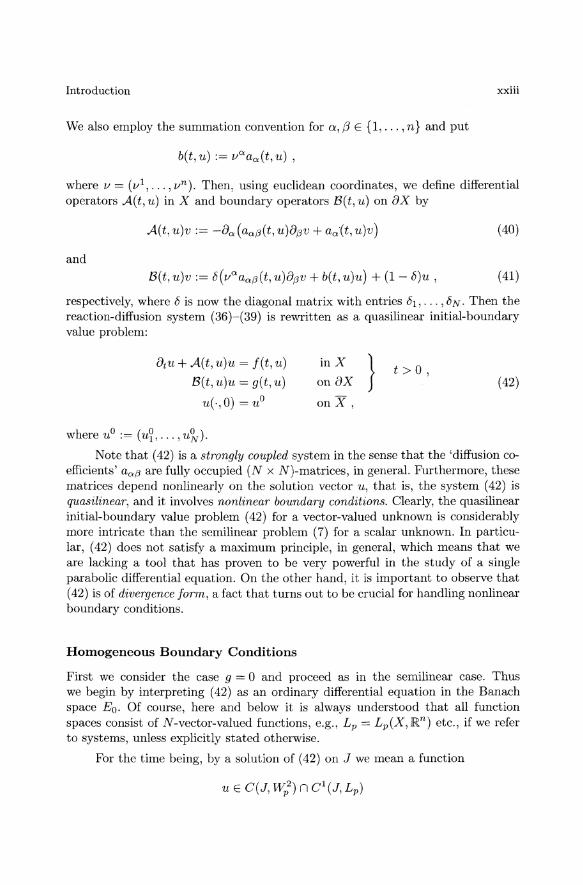
We also employ the summation convention for a, (3 E {I, ... , n} and put

b(t,u) := vQ;aa(t,u) ,

where v = (v1 , ... , vn). Then, using euclidean coordinates, we define differential operators A(t, u) in X and boundary operators 8(t, u) on 8X by

(40)

and

8(t, u)v := 6(vaaa(3(t, 71)8(3v + b(t, u)u) + (1 - 6)u , (41)

respectively, where fj is now the diagonal matrix with entries fjl, ... ,6 N. Then the reaction-diffusion system (36)~(39) is rewritten as a quasilinear initial-boundary value problem:

8t u + A(t, u)u = f(t, u)

8(t,u)u = g(t,u)

u(.,O) = U o

where U O := (u~, ... ,u~).

in X

on8X

onX,

} t > 0, (42)

Note that (42) is a strongly coupled system in the sense that the 'diffusion co­efficients' aa(3 are fully occupied (N x N)-matrices, in general. Furthermore, these matrices depend nonlinearly on the solution vector u, that is, the system (42) is quasilinear, and it involves nonlinear boundary conditions. Clearly, the quasilinear initial-boundary value problem (42) for a vector-valued unknown is considerably more intricate than the semilinear problem (7) for a scalar unknown. In particu­lar, (42) does not satisfy a maximum principle, in general, which means that we are lacking a tool that has proven to be very powerful in the study of a single parabolic differential equation. On the other hand, it is important to observe that (42) is of divergence form, a fact that turns out to be crucial for handling nonlinear boundary conditions.

Homogeneous Boundary Conditions

First we consider the case g = 0 and proceed as in the semilinear case. Thus we begin by interpreting (42) as an ordinary differential equation in the Banach space Eo. Of course, here and below it is always understood that all fUIlction spaces consist of N-vector-valued functions, e.g., Lp = Lp(X, ]Rn) etc., if we refer to systems, unless explicitly stated otherwise.

For the time being, by a solution of (42) on J we mean a fUIlction

xxiv Introduction

satisfying (42) in the obvious 'point-wise' sense. Given such a solution u, we put

A(t,u(t)) := A(t,u(t))I~~B(t,u(t)) ,

thereby using the notation of (17). Then u is, at least formally, a solution on J of the quasilinear Cauchy problem

u + A(t,u)u = f(t,u) , t E j , u(O) = Uo .

Letting Au(t):= A(t,u(t)) , t E J ,

u is also a solution of the nonautonomous semilinear Cauchy problem

V+Au(t)v=f(t,v) , tEj, v(O) = uo .

Hence it can be expressed by the variation-of-constants formula

u(t) = Uu(t,O)uO + It Uu(t,T)f(T,U(T)) dT, t E J,

(43)

(44)

(45)

where now the semigroup in (24) is replaced by the evolution operator Uu of the family {Au(t) ; t E J}. Consequently, denoting by <I> the right-hand side of (45), we are again led to the fixed point equation (27) that we want to make the basis for our study of the quasilinear problem (43).

Now the situation is much more complex than in the semilinear case. First of all, to give a meaning to these formal considerations we have to guarantee the existence of the evolution operator Uu , given a function u possessing suitable regularity properties. Clearly, the existence and the properties of an evolution operator are intimately related to the solvability of the linear Cauchy problem

v + A(t)v = f(t) , t E j , v(O) = UO , (46)

that is obtained from (44) by ignoring the u- and v-dependence of A and f, re­spectively, for the moment. This Cauchy problem corresponds to a Banach space formulation of the nonautonomous linear initial-boundary value problem

8tv + A(t)v = f(t)

B(t)v = 0

v(·,O) = uO

in X } on8X

onX,

t > 0,

where now the coefficients in (40) and (41) are independent of u.

(47)

In the simplest case of a scalar unknown, that is, for N = 1, we know already from (17) and (22) that

A(t) E 1t(El(t), Eo) , (48)

where

El (t) ~ ~~B(t) . (49)

Note that (48) means that each A(t) is the negative generator of an analytic semigroup on Eo, whose domain is t-dependent, in general.

Introduction xxv

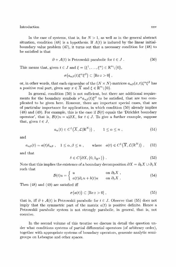
In the case of systems, that is, for N> 1, as well as in the general abstract situation, condition (48) is a hypothesis. If A(t) is induced by the linear initial­boundary value problem (47), it turns out that a necessary condition for (48) to be satisfied is that

a + A(t) is Petrowskii parabolic for t E J .

This means that, given t E J and ~ = (e, ... , ~n) E lRn \ {O},

u(aa(3(t)~a~(3) C [Rez > 0] ,

(50)

or, in other words, that each eigenvalue of the (N x N)-matrices aa(3(x, t)~a~(3 has a positive real part, given any x E X and ~ E lRn \ {O}.

In general, condition (50) is not sufficient, but there are additional require­ments for the boundary symbols v""aa(3(t)e to be satisfied, that are too com­plicated to be given here. However, there are important special cases, that are of particular importance for applications, in which condition (50) already implies (48) and (49). For cxample, this is the case if B(t) equals the 'Dirichlet boundary operator', that is, B(t)u = ulax, for t E J. To give a further example, suppose that, given t E J,

(51)

and

aa(3(t) = a(t)8a(3, 1:S: a,/3:S: n , (52)

and that (53)

Note that this implies the existence of a boundary decomposition ax = aox u a1x such that

B(t)u = { ~(t)a,/U + b(t)u

Then (48) and (49) are satisfied iff

u(a(t)) C [Rez > 0] ,

(54)

(55)

that is, iff a + A(t) is Petrowskii parabolic for t E J. Observe that (55) does not imply that the symmetric part of the matrix a(t) is positive definite. Hence a Petrowskii parabolic system is not strongly parabolic, in general, that is, not coercive.

In the second volume of this treatise we discuss in detail the question un­der what conditions systems of partial differential operators (of arbitrary order), together with appropriate sy~tems of boundary operators, generate analytic semi­groups on Lebesgue and other spaces.

xxvi Introduction

Constant Domains

Now let conditions (48) and (49) be satisfied. Then, to guarantee the existence of an evolution operator U for the linear Cauchy problem (46), one has to impose regularity assumptions on the function t f--+ A(t). It turns out that the required amount of regularity is proportional to the 'strength of variability' of the domains of A(t), that is, the spaces El (t), if t varies over J.

The simplest case occurs if the domains of A(t) are independent of t E J, that is, if El(t) ~ El(O) =: El for t E J. Note that this is the case if B(t) equals the Dirichlet boundary operator for t E J. It is also true if conditions (51)-(55) are satisfied and b = 0, since in this case the homogeneous boundary condition B(t)u = 0 is equivalent to the constant boundary condition 80v u + (1 - 8)u = 0 on aX.

If the operators A(t) have a constant domain E l , it suffices to require that

(56)

for some p E (0,1). Then there exists a unique evolution operator U for the family {A(t) ; t E J} such that each solution of (46) can be represented by the variation­of-constants formula

u(t) = U(t,O)uO + lot U(t,T)f(T)dT, t E J .

Furthermore, the evolution operator U possesses properties that are similar to the ones of the semigroup {e- tA ; t 2:: O} of the autonomous problem. In particular, the following analogue of (29) is valid:

IIU(t, 8)llc(Eo,EIl ::; c(t - 8)-1 , t,8 E J, 8 < t .

Recall that our interest belongs to the quasilinear equation (43), and thus to the fixed point equation (45). Since the dependence of A on u in (43) implies a dependence of U on u in (45), it is necessary to study carefully the dependence of U on A. The construction of the evolution operator, as well as the investigation of its dependence on A, is the content of the second chapter of this volume. There the general setting of an arbitrary densely injected Banach couple is considered, which greatly enhances the applicability of our results.

Of course, treating the quasilinear problem (43) by reducing it to the fixed point equation (45), we encounter the same difficulties we found when we had to give a meaning to the fixed point map <I> in the semilinear case (13). Thus we have to consider again an 'intermediate' space Ea satisfying (31) such that each one of the semigroups {e-tA(s) ; t 2:: O}, 8 E J, restricts to a strongly continuous semigroup on Ea and (32) is replaced by

IIU(t, 8)llc(Eo,Eu) ::; c(t - s)-a , t,8 E J, 0::; 8 < t .

Introduction XXVll

As in the semilinear case, D(AO!(O)) seems to be a natural candidate for Ea. However, this choice is not the best one, mainly since D(AO!(t)) is not known ex­plicitly for a E (0,1). Thus, for example, it is not elear if D(AO!(t)) is independent of t E J, in general.

Although it is possible to develop a general theory of abstract quasilinear Cauchy problems by basing it on the theory of fractional powers - this has been done by P.E. Sobolevskii in [Sob66] (also cf. [Fri69] for an exposition of parts of that work) - , this approach does not give optimal results. Indeed, by Sobolevskii's approach it is not possible to prove that the solutions of (43) generate a semiflow, that is, a nonlinear local semigroup, since one has to require more smoothness for the initial datum U O than should be expected. In other words, the initial value U O

has to belong to a slightly smaller space than the natural phase space of (43).

The semiflow property of the solutions of the abstract quasilinear Cauchy problem is both natural and fundamental for a qualitative study of the latter. Thus any good general theory has to produce this property. Therefore we are forced to look for other candidates for EO!. Fortunately, there are plenty of them: most of the interpolation spaces of exponent a between Eo and El turn out to lead to the desired results. Thus at this stage interpolation theory comes into play naturally.

Together with the theory of analytic semigroups, interpolation theory plays a predominant role in the abstract theory of linear and quasilinear Cauchy problems of 'parabolic type'. For this reason we collect in Chapter I the basic facts from these two fields, that are being used throughout our treatise. Furthermore, concrete characterizations of interpolation spaces are studied in detail in the second volume. In particular, the following is shown: let

and put

{ v E WP" ; B(t)v = O} , { v E WP" ; (1 - 8)v18X = O} ,

Wp",

1 + lip < 8 < 00 ,

lip < 8 < 1 + lip, 0::;: 8 < lip,

W;'S:= W;'S(t) , S E [0,1 + IIp)\{llp}·

(57)

Then, given a E (0,1) with 2a ~ {lip, 1 + lip}' there exists an interpolation func­tor (-, .)" of exponent a such that

(58)

where Eo := Lp and El(t) := ~~S(t) = dom(A(t)). Note that E" := E,At) is in­dependent of t E J if 0 < 2a < 1 + lip and 2a i= lip.

The assumption of constant domains for A (t, u( t)), which entails the inde­pendence of the interpolation spaces Eo(t) of t E J, simplifies the approach to quasilinear parabolic problems considerably and results in a rather flexible theory.

XXVlll Introduction

This is essentially due to the fact that the existence of an evolution operator can be guaranteed by presupposing (56) with an arbitrarily small Holder exponent p. As a rule, A(t,u(t)) is well-defined only if 11,(t) belongs to E(3 for (3 sufficiently large. Indeed, to guarantee (49) we have to assume that

a,(3E{l, ... ,n}, tEJ.

Thus we certainly have to require that u E C 1 . Consequently, we infer from (56) that we have to assume that

(59)

where E(3 ~ C 1 . By (18), (57), and (58), for this embedding to be valid we have to impose the condition (1 + nip) < 2(3 < 2, which entails p> n. Now we fix a E ((3,1) and choose Ea as a phase space, that is, we study the fixed point equation (45) in C(J, Ea). Then <I> maps C(J, Ea) into C(J, EaJ n CP(J, E(3), pro­vided p < a - (3. Hence U1 := <I>(11,) satisfies (59) whenever 11, E C(J, Ea). So the iteration process of the method of successive approximations can be carried out in­definitely, and it can indeed be shown that <I> has a unique fixed point in C(J, Ea), provided J is sufficiently short. Note that this imposes the restriction 2p < 1 - nip. It should also be remarked that, up to this point, the divergence structure of (40), (41) is not needed.

Extrapolation Theory

The approach outlined above uses in an essential way the fact that the domains of A(t) are constant. More precisely, it is based on the fact that the interpolation spaces E(3 and Eo: are independent of t for 1 + nip < 2,6 < 2a < 2. By (57) and (58), this is not the case if dom(A(t)) = ~~S(t) depends on t E J.

On the other hand, thanks to its divergence structure, problem (42) has a natural weak formulation. For this put

(v, wI := Lv, W dx , (v,W) E Lp' x Lp .

Furthermore, given t E J and 'U E C, let

Then a(t,11,) is a continuous bilinear form on W~ s x Wp1s, the 'Dirichlet form' p, ,

belonging to (A(t, 11,), B(t, 11,)). Thus, letting

-2 + lip < s < 0, s I- -1 + lip, (60)

with respect to the duality pairing naturally induced by the Lp-duality pair­ing (', 'I, it follows that a(t,11,) induces

A(t, 11,) E .c(Wp~s, WP~J) (61)

Introduction

via (v,A(t,u)w):= a(t,u)(v,w) , (v, w) E Wd',B x ~:,B .

We abo define a nonlinear map F by

(v,F(t,u)):= (v,f(t,u))+ r v·g(t,u)dIJ, Jax v E Y~~,B .

xxix

(62)

(63)

Then, thanks to the divergence structure of (40) and (41), the natural weak for­mulation of the initial-boundary value problem (42) takes the form:

find u E C(J, Wp~B) satisfying

1 { -(v, u) + a(t, u)( v, u)} dt = 1 (v, F(t, u)) dt + (v(O), uo) (64)

for each v E cl(J, ~~,B) vanishing near the right endpoint of J.

It is easily seen that every solution of the initial-boundary value problem (42) is a weak solution in the sense of (64). Furthermore, (64) is equivalent to the abstract quasilinear Cauchy problem in W-J: p,

u+A(t,u)u=F(t,u) , tE j, u(O) = Uo . (65)

Observe that, thanks to (61), the domains of the operators A(t, u) are all equal to Wp~B' Thus (65) is amenable by the techniques described above for the constant domain problem (43), provided

(66)

with suitably regular dependence on (t, u).

It is a consequence of the divergence theorem that A(t, u) is an extension of

A(t, u) := A(t, U)IW;'B(t,u) .

This fact can be used to prove (66). To outline this method, we first fix a negative generator B of a strongly continuous analytic semigroup on an arbitrary Banach space Fo := (Fo, 11·110) and assume, for simplicity, that B has a bounded inverse defined on Fa. Then

defines a norm on dom(B) that is equivalent to the graph norm. This implies that FI := (dom(B), 11'111) is a Banach space such that (Fo,F1 ) is a densely injected Banach couple, and B E H(Fl' Fo).

The Banach space Fo can be recovered from Fl by observing that Fo is a completion of Fl in the norm u f--> IIB11'ulil = Ilullo, where Bl is the Fl-realization

xxx Introduction

of B. This suggests to introduce a superspace F-l := (F-l' 11·11-1) of Fo by choos­ing for

F-l a completion of Fo in the norm u t-+ IIB- 1ullo =: Ilull-I.

Then (F -1, Fo) is a densely injected Banach couple as well, and it is not difficult to show that Bo := B extends continuously to an operator B-1 E H(Fo, F-1). If B is not invertible, we simply replace B by w + B for a sufficiently large w E lR+.

Now, given () E (0,1), we choose an interpolation functor (., ·)0 of expo­nent () with the property that Gl is dense in (Go, Gt}o whenever (Go, G1 ) is a densely injected Banach couple, an 'admissible interpolation functor'. Then we put Fe := (Fo, Ft)o and FO-l := (F-l' Fo)o. This defines a 'scale of Banach spaces'

-1<,6<0<1.

Furthermore, denoting the Fa_I-realization of B-1 by B a - 1 for 0 E [0,1], it follows that

Ba - 1 E H(Fa , Fa-t) ,

These extensions are 'natural' in the sense that e-tB"'-l is the restriction to Fa - 1

of e- tBj3 - 1 for 0 :S f3 < 0 :S l. This 'interpolation-extrapolation' technique is rather flexible, has many ap­

plications, and is crucial for our approach to quasilinear parabolic evolution equa­tions. It allows to measure very precisely regularity properties of operators and solutions. Scales of Banach spaces, interpolation-extrapolation techniques, and evolution equations in these scales are studied in detail in Chapter V.

Now we return to our quasilinear parabolic problem. In this case, given (t, u), we can construct an interpolation-extrapolation scale by starting with A(t, u) on Eo = Lp- Then, using suitable admissible interpolation functors, this scale, denoted by Ea(t, u) for 0 E [-2,1]' can be explicitly represented as

Ea(t, u) ~ ~~B(t,u) , 20 E (-2 + lip, 2]\(Z + lip) ,

in the range given. Thus we infer from (57) and (60) that

20 E (-2 + lip, 1 + 1/p)\(Z + lip) . (67)

Therefore the interpolation-extrapolation spaces are independent of (t, u), that is, they are constant, if 0 belongs to the range given in (67). Moreover, denoting by A a - 1(t,u) the 'extrapolated operators', the general theory of Banach scales tells us that

Aa-l (t, u) E H(E", , Ea-l) ,

Lastly, it can be shown that

lip < 20 < 1 + lip·

A(t, u) = A-1/ 2 (t, u) ,

which, thanks to (67) and (68), proves (66).

(68)

(69)

Introduction xxxi

Regularity

The interpolation-extrapolation technique outlined above enables us to solve the initial-boundary value problem (42) in its weak form (64), provided a and Fare suitably regular. In fact, it suggests to replace the quasilinear evolution equa­tion (65) by the family

u+Aa-l(t,u)u=F(t,u) , tEj, u(O) = uo (70)

for l!p < 2a < 1 + l!p. In particular, we can fix 2a E (1,1 + l!p) and can choose E l / 2 = Wp~B as a phase space for the constant domain problem (70). Then, given uo E El/2' problem (70) has a unique maximal solution

° . 1 . 'Un := u(·, u ) E G(Jo, El/2) n G(Jo, En) n G (Jo, Ea- l ) . (71)

It follows from (69) and A-l/2 ~ Aa- l that Uo is a weak solution of (42) in the sense of (64). But (71) shows that Uo possesses better regularity properties.

This observation suggests a bootstrapping procedure. For this we observe that Uo is a solution of the linear Cauchy problem

v + A, -1 ( t, Uo ( t )) = F ( t, Uo ( t )), t E j ° , v(O) = uo

in En-I. Recall that A,-l(t,uo(t)) ~ A,6-l(t,U(t)) if {3 > a. Thus, if the linear Cauchy problem

v + A,6-l (t, uo(t))v = F(t, uo(t)) , t E jo , v(O) = uo (72)

is well-posed in E,6-l for some {3 E (a,l], its solution coincides with un. Note that a solution u of (72) satisfies u(t) E dom(AB-l(t,Uo(t))) for t E jo. Hence it follows that

uo(t) E dom(A,6-l(t,UO(t))) C Wp2,6-2

for t E jo, provided (72) is well-posed.

By these considerations we are led to study the linear Cauchy problem

iJ + A,6-l(t)V = F(t) , t E j ,

(73)

in E,6-l, where we are particularly interested in the case 2{3 > 1 + l!p, so that dom(A,6-l(t)) is no longer constant. Since Aa-l(t) :J A,6-l(t), it is to be expected that the restriction of the evolution operator Un - l of the family { Aa - l (t) ; t E J} to the space E,6-l '--+ Ea - 1 is an evolution operator for { A iJ - l (t) ; t E J} on E,6-l. This is true in fact, provided

p>{3-a, (74)

as follows from the general results derived in Chapter IV.

xxxii Introduction

It turns out that Aa-1(t,uo(t)) can be characterized, similarly as A-1/2(t) in (69), through the bilinear form a(t,uo(t)), the latter now being continuout; on Wp~~B2a X ~~B' A careful study of point-wise multipliers on generalized Sobolev spaces, that is carried out in the second volume, reveals that

(75)

if (J > 20: - 1. From (71) we infer, using suitable embedding theorems, that

Uo E CP (Jo , C(1) , (76)

provided 2p < 20: - (J - nip. By combining (75) and (76) we see that

(77)

for 2p < 1 - lip. Hence A a - 1 (" uo(-)) satisfies (74) for

2(3 < 20: + 1 - nip < 2 - (n - l)lp .

This way, and using the theory developed in Chapter IV, it follows that

. 2/3 l' 2/3 2 . Uo E C(Jo, Wp ) n C (J, Wp,B - ) '--+ CP(J, C(1) ,

provided 2(3 < 2 - (n - l)/p and (J + 2p < 2(3 - nip < 2 - (2n - l)/p. Thus, since we can choose an arbitrarily large value for p, we obtain

(J + 2p < 2. (78)

At this stage we can invoke the classical Holder theory for general parabolic sys­tems, for example, to deduce that Uo is in fact a classical solution, even a Coo_ solution, of the initial-boundary value problem (42).

Unfortunately, the situation is more complicated than just indicated. First, in the preceding outline we neglected the difficulties coming form F(t,uo(t)). The

above procedure requires t f--+ F( t, uo(t)) to belong to C(1 (J, E/3-1) for (3 arbitrarily close to 1. This does not hold, in general, unless the boundary nonlinearity 9 satis­fies appropriate compatibility conditions and the problem is suitably modified. For the latter modification one has to have a good theory of nonhomogeneous linear parabolic boundary value problems in W; for 1 + lip < s ::; 2 under mild regular­ity conditions on the coefficients. These questions are investigated in Volume Two.

Second, it is by no means clear that Aa_1(t,uo(t)) E 1-i(Ea, Ea- 1) ifuo sat­isfies (76). Indeed, to derive (68) we started with A(t, u) E 1-i (E1 (t, u), Eo). In our concrete situation this can only be established if the coefficients of .A and B are of class C 1 . To guarantee this we would already have to know that Uo (t) E C 1 .

Thus we have to prove directly that -A",_1(t,U) generates a strongly continuous analytic semigroup on E a - 1 if .A and B have Holder continuous coefficients only.

Introduction xxxiii

This problem is also studied in detail in the second volume by making use of the interpolation-extrapolation technique for smooth operators.

Having established the necessary ingredients, the above bootstrapping tech­nique can be carried through, in principle. However, the technical details are some­what delicate, and it is not possible, in general, to derive (78) in one step. Instead, a chain of bootstrapping arguments is needed. These arguments are given in detail in the third volume on the basis of the results of Volume Two.

Besides of existence and regularity theorems, in the last volume a qualitative theory of quasilinear parabolic evolution equations is developed as well. It is shown that they generate smooth local semiflows on appropriate natural phase spaces. Furthermore, questions of global existence, stability of critical points and periodic orbits, bifurcation phenomena, etc., are studied in the general abstract setting. In addition, those results are applied to a variety of concrete systems of partial dif­ferential equations stemming from diverse applications in physics, chemistry, etc.

Maximal Regularity

The theory of linear and quasilinear parabolic evolution equations, outlined so far, uses crucially the smoothing property of parabolic equations. This regularizing effect is the ultimate reason for the validity of global existence theorems based on a priori estimates in 'weak' norms, that is, norms involving little regularity of the solutions only.

On the other hand, it restricts the applicability of the general abstract theory to quasilinear reaction-diffusion systems whose 'diffusion matrices' depend on u only, at least in the divergence form case. If grad u also occurs in the diffusion matrices, this theory is not applicable since it uses the fact that the dependence of Ac,,-l (t, u) E £( E et , Ea - l ) on (t, u) is smooth with respect to the topology of an interpolation space (Ea- l , Ea)o that is strictly weaker than the topology of Ea.

If the 'intermediate' smoothness requirement is not satisfied, e.g., if the diffu­sion matrices depend on grad u, we have to invoke maximal regularity results. The maximal regularity approach is different in spirit from the evolution operator ap­proach discussed so far. Whereas the latter is essentially a dynamical method, that is the infinite-dimensional analogue to the theory of ordinary differential equations, the former is basically a stationary technique. This means that the linear Cauchy problem (46) is interpreted as an 'algebraic' equation in a suit­able Banach space lEo such that lEo '--+ Ll (J, Eo). To be more precise, we consider the case of constant domains and suppose that lEl is a Banach space such that lEI '--+ Ll (J, E l ) n wI (J, Eo) and 8 + A E £(lEl' lEo). Of course,

(8 + A)u(t) := u(t) + A(t)u(t) , u E lEo, a.a. t E J .

Moreover, putting rU : = u( 0) for u E lEI, let r lEI be the 'trace space' of r such that El '--+ rlEl '--+ Eo and r is a continuous surjection from lEI onto rlEl. Then,

xxxiv Introduction

given (j, uO) E lEo X /,lEI, we rewrite the linear Cauchy problem (46) in the form:

find u E lEI such that (8 + A, /,)u = (j, U O).

Finally, the pair of Banach spaces (lEo, lEI) is said to be a pair of maximal regularity for {A(t) ; t E J}, provided (8 + A, 'I) is a topological isomorphism from lEI onto lEo x /,lE l . If this is the case, it is to be expected that we can apply linearization techniques based on the implicit function theorem to solve the quasilinear Cauchy problem (43), that now takes the form of the nonlinear operator equation

In fact, this way 'fully nonlinear problems' can be handled. However, in the quasilinear situation we can combine the maximal regularity approach with the interpolation-extrapolation method to deal with the case of nonconstant domains as well. Indeed, in the qualitative study of quasilinear evolution equations a com­bination of the dynamical evolution operator approach and the maximal regularity technique, used in the third volume, gives the best results.

It turns out that the requirement that (lEo, lEI) be a pair of maximal regu­larity for {A(t) ; t E J} imposes restrictions on the spaces and on the operators, in general. These questions are carefully discussed in Chapter III, where the most important and useful abstract maximal regularity results are derived. Concrete re­alizations necessitate rather deep information on various function spaces, Nikols'kii spaces, for example, and on linear elliptic differential operators. This is provided in the second volume.

The Scope of the Theory

By now the reader surely feels that our approach to the quasi linear initial-boundary value problem (42) is rather lenghty, highly complicated, and requires a lot of tech­nical details. This being certainly true, one might wonder if it is worthwhile at all.

Of course, there are simpler methods for proving the existence of weak so­lution to problem (42). First, the theory of monotone operators can sometimes be applied. However, it requires rather stringent conditions for the operators and nonlinearties and applies to a small class of problems only, leaving aside most systems of interest.

Second, there is the Galerkin approximation approach, that is perhaps most often applied to produce weak solutions of problem (42). That method is basically a Hilbert space technique, being based on coercivity estimates. However, coercivity estimates do not hold for general Petrowskii parabolic systems. To guarantee coer­civity estimates one has to restrict the consideration to certain 'strongly parabolic' systems, a class that is too narrow to cover many interesting problems occurring in science. Similar statements hold for other (space or time) discretization methods.

Introduction xxxv

Even if the system is strongly parabolic, so that the Galerkin method is available, that approach gives weak Wi-solutions only, that is, solutions in the sense of (64) with p = 2. However, it is well-known (e.g., [Gia83]) that weak wi­solutions of systems are not regular, in general. In fact, it is not even possible, as a rule, to prove that they are HOlder continuous. This lack of regularity renders it rather difficult - if not impossible - to develop a dynamical systems theory and to use techniques from nonlinear analysis to establish qualitative properties of the solution set.

In contrast, our approach applies to noncoercive problems as well and gives weak Wp1-solutions, where p > n. Thus, thanks to (18), the solutions we find are already known to be Holder continuous from the very beginning. As indicated above, this implies that all our solutions are classical if all data are sufficiently smooth. Of course, there may be singular solutions - in particular, if the coeffi­cients of A and B lack regularity - that we 'do not see' in our approach. However, we obtain a completely satisfactory local theory in the class of regular functions. It tells us, roughly speaking, that the quasilinear Cauchy problem (43) has the same behavior - as far as local existence and continuous dependence of the solutions on the data are concerned - as an ordinary differential equation:iJ = 'P(t, y) in the finite-dimensional setting. In addition, since our solutions are weak Wi-solutions as well, they coincide on the common interval of existence with weak vVi-solutions obtained by any other method, provided there is a uniqueness theorem for weak Wi-solutions.

In addition, our approach is general. It is by no means restricted to second order reaction-diffusion systems, but applies to quasilinear systems of Petrowskii parabolic type of arbitrary order. Furthermore, the coefficients of A and B, as well as the nonlinearities, can be nonlocal functions. This allows to deal rather easily with elliptic-parabolic systems, for example, by reducing them to abstract parabolic evolution equations. The general abstract theory can also be applied to produce nontrivial results for free boundary value problems, and to systems with 'dynamic boundary conditions'. It can handle 'highly degenerate' problems that are not even Petrowskii parabolic, as well as quasilinear parabolic problems involving pseudodifferential operators. Thus, at the end, we are rewarded by a rather flexible general theory that requires the verification of a few hypotheses only. Those can be met in many concrete situations occurring in applications, as is demonstrated by the examples given in the third volume.

\Venn Du wissen willst, was bewiesen wurde, schau den Beweis an. 5

Ludwig Wittgenstein (1889-1951)

5If you want to know what has been proven, study the proof.