Monitoring Streambed Scour/Deposition Using Non-Sinusoidal Water Temperature Signals

and During Flood Events

A Thesis

Presented in Partial Fulfillment of the Requirements for the

Degree of Master of Science

with a

Major in Civil Engineering

in the

College of Graduate Studies

University of Idaho

by

Timothy R. DeWeese

Major Professor: Daniele Tonina, Ph.D.

Committee Members: Ralph Budwig, Ph.D.; Charles Luce, Ph.D.

Department Administrator: Richard Nielson, Ph.D.

July, 2015

ii

Authorization to Submit Thesis

This thesis of Timothy R. DeWeese, submitted for the degree of Master of Science in Civil

Engineering and titled “Monitoring Streambed Scour/Deposition Using Non-Sinusoidal Water

Temperature Signals and During Flood Events,” has been reviewed in the final form.

Permission, as indicated by the signatures and dates below, is now granted to submit final

copies to the College of Graduate Studies for approval.

Major Professor: _________________________________ Date: _______

Daniele Tonina, Ph.D.

Committee Members: _________________________________ Date: _______

Ralph Budwig, Ph.D.

_________________________________ Date: _______

Charles Luce, Ph.D.

Department

Administrator: _________________________________ Date: _______

Richard Nielson, Ph.D.

iii

Abstract

Streambed erosion and deposition are inherent to river beds, and monitoring their evolution is

important for ecological system management and instream infrastructure stability. The

thermal scour-deposition chain (TSDC) is a novel tool capable of simultaneously monitoring

scour and deposition, stream sediment thermal regime, and seepage velocity information, but

previous research did not address non-sinusoidal temperature variations and natural flooding

conditions. Laboratory tests show the TSDC is equally capable of measuring scour-deposition

sequences and seepage velocity using sinusoidal and non-sinusoidal temperature signals under

a range of seepage velocities. Application in a dam release stream during flood condition

shows excellent match between surveyed and TSDC-monitored bed elevation changes and

provides useful seepage velocity information even under very low temperature signal

amplitudes. Future research should focus on improved techniques for temperature signal

phase and amplitude extractions, as well as TSDC application to monitor scour at bridge piers

and abutments.

iv

Acknowledgements

There are a number of people and organizations to whom I owe my greatest appreciation.

Without them, this work would not have been possible. I would like to thank my advisor,

major professor, and mentor Dr. Daniele Tonina for his much needed guidance and patience

through the entire process of writing research grants, experiment design, data collection and

analysis, and completion of this thesis. He was available whenever I needed him, which

cannot be easy given his busy schedule. Dr. Charles Luce provided much needed technical

support when air bubbles were my nemesis and mathematical genius when data analyses went

awry. The laboratory experiment would have been missing the critical sinusoidal (and non-

sinusoidal) water temperature supply without the many hours of programming by John

Berndt, with Bolen’s Control House in Boise, Idaho. Bob Basham, our lab manager, helped

keep experimental and field equipment design to manageable, constructible levels.

Mohammad Sohrabi and Dr. Daniele Tonina toiled alongside me for hours, pounding those

pesky temperature probes into the rocky streambed. Rohan Benjankar and Jeff Reeder assisted

with field surveying and pebble counts. Dr. Jairo Hernandez at Boise State University called

me during the summer following my undergrad work to be a research assistant. Prior to this

call, I did not see research in my future. There are many folks at Boise State University that

made completing my bachelor’s degree possible. Thank you to them because without the B.S.,

grad school would of course not have been possible. I would like to thank the Hydro Research

Foundation for providing the research award that funded my final year. Brenna Vaughn and

Deborah Linke with the foundation work tirelessly to support students performing research in

fields related to hydropower. Finally, I would like to thank the Idaho State Board of Education

and Idaho Transportation Department for additional project funding.

v

I owe my deepest gratitude to my family, to whom I have dedicated this work. I started as a

freshman at Boise State University in Civil Engineering six years ago and went straight into

grad school at University of Idaho. To complete all of this work in six years in engineering is

a difficult task and consumed much of my non-sleeping time every day and week. My wife

endured many days of doing all of the family and household duties while I studied and

researched. She was my rock, my motivator, and my shoulder to rest on when things got

excessively stressful. And, last but not least, I thank my children. My children were the

absolute biggest motivator of all. Many times I would look at them and realize I am doing all

of this for them, to lead them and to leave them and their children a bright future full of life

and beauty. My father taught me to leave it better than I found it. I have taken this to the full

extent and am doing everything I can to leave the world a better place for my children and

theirs.

vi

Dedication

To my beautiful wife, Julie, I dedicate this work to you as a thank you for all of your much

needed love and support throughout my college education. To my children Averi, Brady, and

Jacob, you are our future. With hard work and dedication to a set of goals, you will do great

things. To my mother and father, Sherry and Frank, thank you for instilling in me the drive

and can’t quit attitude it takes to accomplish a task of this magnitude.

vii

Table of Contents

Authorization to Submit Thesis ................................................................................................. ii

Abstract ..................................................................................................................................... iii

Acknowledgements ................................................................................................................... iv

Dedication ................................................................................................................................. vi

Table of Contents ..................................................................................................................... vii

List of Figures ........................................................................................................................... ix

List of Tables............................................................................................................................. xi

1.0 Introduction ..................................................................................................................... 1

2.0 Methods ........................................................................................................................... 6

2.1 Theory ......................................................................................................................... 6

2.2 Lab Experiment ........................................................................................................... 8

2.3 Field Study Site ......................................................................................................... 13

3.0 Results ........................................................................................................................... 17

3.1 Lab Experiment ......................................................................................................... 17

3.2 Field Study Site ......................................................................................................... 23

4.0 Discussion ..................................................................................................................... 29

5.0 Conclusion .................................................................................................................... 36

viii

References ................................................................................................................................ 38

ix

List of Figures

Figure 1: Field study site. Located 2 miles downstream of Anderson Ranch Dam on the South

Fork Boise River, Idaho, USA. .................................................................................................. 5

Figure 2: Sketch of laboratory experiment............................................................................... 12

Figure 3: Imposed laboratory surface water temperature signals. Experiments A and B used a

sinusoid signal (blue), and experiments C and D used a sawtooth signal (black), both have

same wavelength. ..................................................................................................................... 13

Figure 4: Left: South Fork Boise River study site showing the debris flow that added sediment

to the channel, with approximate thermal scour probe installation locations 1, 2, 3, 4. (Photo

used with permission from the USDA, Boise National Forest); Middle: Field temperature

probe; Right: Temperature probe installed with data logger. .................................................. 16

Figure 5: Pre-flood (blue) and post-flood (red) grain size distribution at South Fork Boise

River locations 1 and 2. Locations 3 and 4 did not experience significant change in grain size

distribution due to little scour or deposition and their grain size distribution remained similar

to the pre-flood condition. ........................................................................................................ 16

Figure 6: Plots from experiment A. a) Example of measured sediment tank temperatures

during a scour period. b) Phase with depth from data in 4a. c) Example of measured sediment

tank temperatures during a deposition period. d) Phase with depth from data in 4c. Vertical

dashed lines in b and d indicate range of depth where data is useful, starting at the bed

location of 0 cm. ....................................................................................................................... 18

x

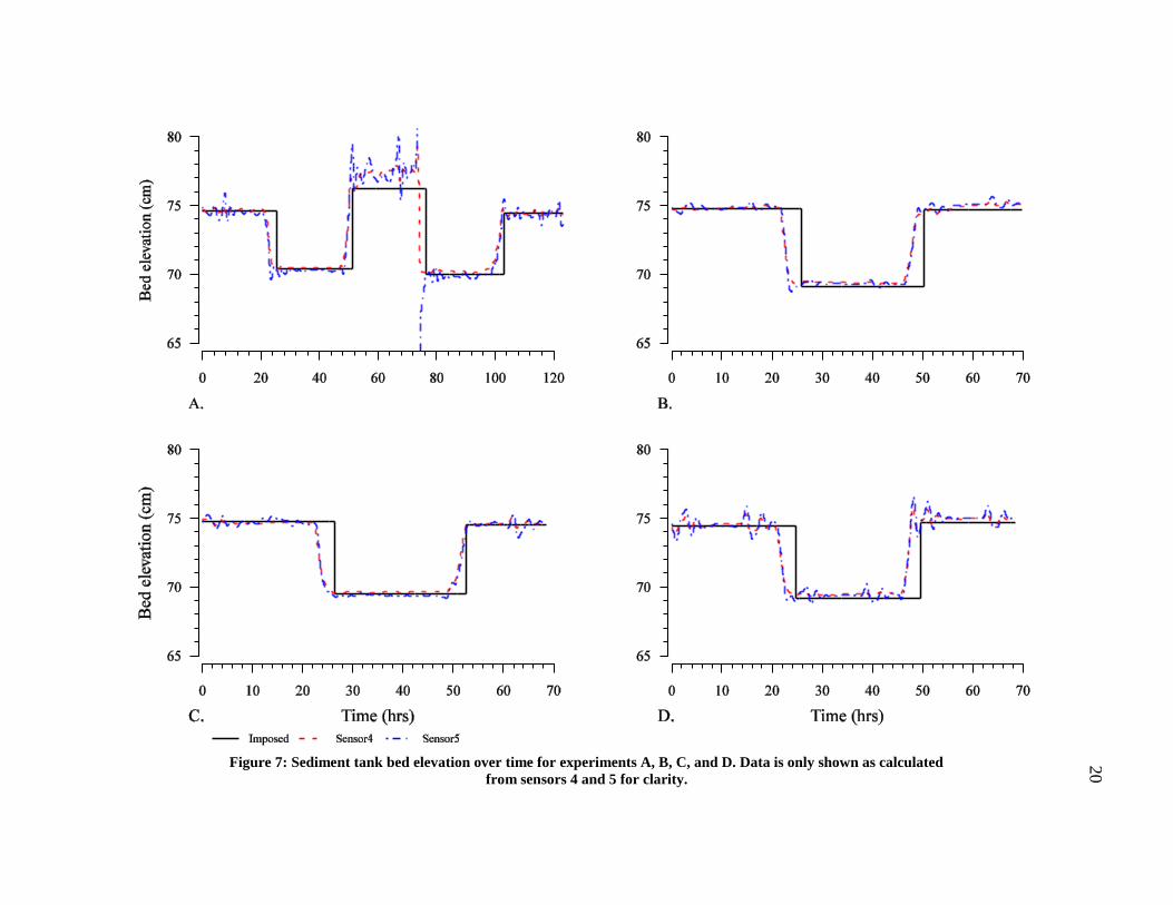
Figure 7: Sediment tank bed elevation over time for experiments A, B, C, and D. Data is only

shown as calculated from sensors 4 and 5 for clarity............................................................... 20

Figure 8: Laboratory experiment calculated and imposed velocities. Shaded regions indicate

time period of scour shown in Figure 7. .................................................................................. 22

Figure 9: Temperature profile measured in the South Fork Boise River at location 1 for the

submerged deployment period. Sensor 1 is at the surface water/sediment interface, and

increasing sensor number represents increased sediment depth in 15 cm increments. ............ 23

Figure 10: South Fork Boise River measured and calculated stream bed elevations along with

the hydrograph released from Anderson Ranch Dam (secondary y-axis, blue line). Locations

1, 2, 3, and 4 are represented by plots a, b, c, and d, respectively. .......................................... 27

Figure 11: South Fork Boise River calculated sediment seepage velocities at each field

location. Depth of temperature sensor increases with increasing sensor number. Locations 1,

2, 3, and 4 are represented by plots a, b, c, and d, respectively. .............................................. 28

xi

List of Tables

Table 1: Laboratory sediment tank experiment velocity, signal type, and temperature signal

amplitude settings for experiments A, B, C, and D. ................................................................ 11

Table 2: Bed elevation RMSE. ................................................................................................ 21

Table 3: Mean calculated velocities and percent error for each sensor in experiments A, B, C,

and D. ....................................................................................................................................... 21

Table 4: Calculated effective thermal diffusivity, κe (cm2 s

-1), for each probe location.

Adjacent pairs are comprised of the listed sensor and the sensor directly above it and provide

vertical variability of κe. Sensors paired to the surface average κe from the repsective sensor

location to the water-sediment interface. ................................................................................. 25

Table 5: Measured and mean calculated streambed elevation changes and associated absolute

error. ......................................................................................................................................... 26

1

1

1.0 Introduction

Hydromorphological dynamicity is inherent to river beds and affects many hydrologic,

geomorphic, and ecological processes within rivers (Gurnell et al., 2012; Knighton, 1998;

Lytle and Poff, 2004; Richards et al., 2002). Research has addressed ecological impacts of

anthropogenic stream channel modifications and associated sediment transport on fish habitat,

benthic organisms, vegetation communities, and others (Newson and Newson, 2000). Among

many human modifications, dams are one example that impacts all of these ecological

categories (Graf, 2006; Knighton, 1998, pp. 307–312; Ligon et al., 1995; Petts and Gurnell,

2005). Adaptive management strategies have been implemented in attempt to reduce

anthropogenic effects in water resource management (Ligon et al., 1995; Richter and Thomas,

2007). Streambed erosion (scour) and deposition also have important implications with

hydraulic structures placed in rivers. Damage to thousands of bridges has been linked to

bridge pier and abutment scour during high flow events (L.A. Arneson et al., 2012). Major

programs have been established to predict and monitor bridge scour to reduce public safety

risk and costly infrastructure loss (Mueller, 1998).

Monitoring channel dynamics is important for both ecological and engineering management

of riverine systems (Maturana et al., 2014). Such information can aid in understanding bi-

directional links among sediment transport and fish habitat, benthic organisms, and vegetation

communities and is important for holistic management of river systems (Marion et al., 2014).

Environmental flows from dams established to minimize negative impacts may result in

scour-deposition events, intended or unintended (Richter and Thomas, 2007). Dam managers

can utilize scour monitoring to quantify the significance of dam re-operation on the riverine

2

2

environment and for verification of desired results. Hydraulic structures susceptible to

streambed scour and deposition can be monitored to provide warning of potential safety

hazards and/or economically catastrophic events (Deng and Cai, 2009). Monitoring at bridge

piers and abutments can be used in conjunction with scour prediction models to provide a

complete system for hazard prevention during flood events.

Several methods have been reviewed for measuring erosion and deposition of stream beds

(Cooper et al., 2000; Deng and Cai, 2009, pp. 129–131; Mueller, 1998; Nassif et al., 2002). A

common and simple method for measuring erosion is the scour chain, which records

maximum erosion during a high flow period and potential subsequent deposition. This method

is time consuming, difficult to install and remove, and provides no timing of measured

erosion and deposition. Other methods have been explored including the magnetic sliding

collar, piezoelectric probes, heat dissipation gauges, photo-electric cells, and conductance

probes. Sonar, radar, time-domain reflectometry, and fiber Bragg grating sensors have also

been implemented to monitor erosion and deposition continuously (Manzoni et al., 2011).

Limitations of these technologies include deployment costs and difficulty deploying large

sensor networks to obtain a distributed erosion-deposition pattern.

A newly developed method uses temperature as a tracer to monitor streambed erosion and

deposition (Gariglio et al., 2013; Luce et al., 2013; Tonina et al., 2014). This method, referred

to as the thermal scour-deposition chain (TSDC), is similar to a technique used for measuring

sediment pore water flux associated with surface water–groundwater exchange and hyporheic

flows (Gariglio et al., 2013; Hatch et al., 2006; Keery et al., 2007; Lautz, 2012, 2010; Rau et

al., 2012; Stallman, 1965). Previous research shows that this new method has several

advantages over existing methods: (1) it uses proven, robust and economical temperature

3

3

sensing technology; and (2) it can simultaneously be used to quantify stream sediment thermal

regime, thermal properties, and sediment seepage velocity. Such advantages make the TSDC

not only a very useful scour monitoring tool but also a tool for improving understanding of

ecological implications due to dam operation and environmental flow regimes.

The TSDC was previously tested under limited imposed scour and deposition sequences with

well-defined sinusoidal daily temperature oscillations, lack of vertical thermal gradients, and

under low, near stationary surface flows (Tonina et al., 2014). While previous results showed

reasonable proof of concept under this scenario, the method should be tested in natural

systems where scour and deposition occur in association with changing discharge.

Furthermore, previous research has indicated uncertainty may arise when using the

temperature methods to analyze streambed water flux due to non-sinusoidal signals of

temperature and vertical thermal gradients (Lautz, 2010). Because TSDC uses the same

mathematical framework and imposed boundary conditions, sinusoidal forcing and

zero-thermal gradient at the two ends of the domain respectively, this research expects to

detect similar inaccuracies when using non-sinusoidal temperature signals for measuring

erosion and deposition with the TSDC. Consequently, this study was designed to address two

fundamental questions regarding the applicability of the TSDC: (1) Will a non-sinusoidal

temperature signal provide results similar to the sinusoidal signals? and (2) How well does the

method perform in a natural system during high flow events?

To address question 1, a laboratory sediment tank was designed, which mimics natural stream

processes, including a cyclic surface water temperature signal, sediment vertical pore water

flux, and scour/deposition sequences. A programmable logic controller (PLC) controls the

surface water temperature, imposing sinusoidal and sawtooth (non-sinusoidal) wave signals.

4

4

The advantages of the laboratory sediment tank are the possibility to impose erosion and

deposition sequences accurately and precisely, as well as vertical seepage fluxes and to avoid

outside influences on errors in physical measurement (e.g. animals scouring the bed).

A field study was performed to address question 2. The South Fork Boise River (SFBR) was

selected, 2 miles downstream of Anderson Ranch Dam (Figure 1). This site was chosen

because of (1) recent massive alluvial deposits from tributaries and (2) planned flow regime to

flush the alluvial deposits, which would enhance the opportunity to monitor changes of bed

elevation. While high flows are not due to natural flooding, scour/deposition sequences that

occur are natural and linked to dam operation and water resource management strategies.

5

Figure 1: Field study site, located 2 miles downstream of Anderson Ranch Dam on the South Fork Boise River, Idaho,

USA.

6

6

2.0 Methods

2.1 Theory

Sediment elevation changes are quantified using a mathematical method based upon one-

dimensional advection and diffusion of temperature (Luce et al., 2013; Tonina et al., 2014),

where phase, , and amplitude, A, of cyclic temperature signals from paired temperature

sensors in the surface water and within the streambed sediment are analyzed (equations 1-3):

Δ

AA

A

η rlnln

12

1

2

(1)

22

2

1

ze (2)

1ez (3)

where η is a dimensionless number relating the natural logarithm of the amplitude ratio,

1

2

A

AAr , to the phase difference between paired temperature signals, Δ .

T

2 , is the

expected angular frequency and T is the period of the temperature signal being analyzed.

Calculation of sediment thickness between temperature sensors, Δz, allows quantification of

bed elevation changes over time. Effective thermal diffusivity, κe, is a thermal property of the

sediment and pore-water matrix and is calculated from the temperature time series obtained

during an intitial, steady state elevation of the bed where Δz is known and constant. This

calculation of κe is different from previous methods (Constantz, 1998; Hatch et al., 2006;

Keery et al., 2007; Lautz, 2012; Swanson and Cardenas, 2010), which require an estimated

value of κe . Once known, κe should remain unchanged through the experiment, thus the value

7

7

is held constant, and Δz over time is calculated. Bed elevations are then calculated by

summing Δz and respective temperature sensor constant elevations.

Seepage velocities, i.e., Darcy velocities, can be calculated at each location once κe is known.

Luce et al. (2013) provide one option for calculating advective thermal velocity independent

of depth:

2

2

1

1

2

d

t

zv (4)

where dz is the diurnal damping depth and is related to κe:

edz (5)

Darcian velocity relates to advective thermal velocity with

tvv (6)

where

ww

mm

c

c

(7)

refers to density and c to specific heat capacity. Subscripts w and m refer to the water and

the sediment pore-water matrix, respectively. Seepage velocity can be calculated by dividing

the Darcian velocity by the sediment effective porosity. Equations 4 through 7 can be

combined to form one equation for seepage velocity related to κe, which is used throughout

the presented analyses:

2

2

1

1

ev (8)

8

8

The analytical solutions behind this mathematical method are similar to those used by

researchers to quantify streambed seepage flux (Hatch et al., 2006; Keery et al., 2007; Lautz,

2012, 2010; Rau et al., 2012; Stallman, 1965). Multiple assumptions behind the analytical

solution have been reported, including (1) sinusoidal temperature signal in the stream surface

water, (2) zero vertical gradient of mean temperature with depth in the streambed, and (3)

equal streambed pore-water and adjacent sediment temperatures. Research has demonstrated

increased error in seepage velocity calculations associated with violations of assumptions 1

and 2 (Lautz, 2010), and excellent results (<1% error) when ideal sinusoidal temperature

signals are analyzed under low or no seepage flow conditions. Research presented in this

paper tests capability of the TSDC to monitor streambed scour and deposition with presence

of violations to these assumptions.

The equations and the signal analysis were coded in the open source statistical computing

environment, R. Numerical analysis uses a discrete Fourier transform (DFT) to extract phase

and amplitude from cyclical temperature time series and combines these extractions with

equations 1 through 8 to obtain bed elevation and velocity data. Bed elevation and velocity

calculations use only measured temperature data and require no parameterizations.

2.2 Lab Experiment

To test the TSDC applicability with non-sinusoidal temperature signals in the laboratory, a

small sediment tank was designed to mimic natural streambed processes. These processes

include: cyclic temperature surface water flow, a sand stream bed with seepage velocity in

both upwelling or downwelling conditions, and scour-deposition sequences. Only

9

9

downwelling experiments are presented in this work. A simple sketch of the laboratory

experiment is provided in Figure 2.

The 40 cm square, 80 cm tall sediment tank is constructed of 3/8 inch clear cast acrylic

sheeting. The tank bottom has two layers, the first of which, with respect to water flowing

down through the tank, is a grid of 100, 3/16” holes that help maintain vertical flow

streamlines through the above sediment matrix. Five centimeters below the grid and 5 cm

above the tank wall bottom is the tank bottom, which has a centered hose fitting for

connection of the downwelling plumbing. This section between the grid and tank bottom is

void of sediment and allows downwelling water to be collected with minimal effect on flow

lines through the sediment. Clear poly (3/8” OD, 1/4” ID) tubing was selected for the

hydraulic system, and flow rate control is accomplished via constant head tanks for supply

and upwelling/downwelling flows.

The surface water supply head tank is fed by the outlet of a controlled temperature mixing

valve, and constant head is maintained through a 1 inch PVC stand pipe drain. Sediment tank

surface water, which mimics the stream flow, flows from the supply head tank, through the

surface water tank and out through a stand pipe drain. Downwelling pore water flow is

induced via a constant head difference from surface water in the sediment tank to drain outlet.

A sand bed is used in the sediment tank. Grain sizes range from 0.178 to 2 mm and median

grain size, d50, of 1.16 mm and total initial sediment depth of 45 cm.

Cyclic source water (i.e. surface water) temperature control is accomplished using an Omron

CP1L-EL20DR-D programmable logic controller (PLC), which operates a Honeywell

MN7505 temperature control actuator on a Honeywell VBN3 mechanical mixing valve.

Temperature control parameters including mean, amplitude, period, and signal type for the

10

10

PLC are selectable through a programmable graphical user interface (GUI) (using Indu-Soft

Web Studio (http://www.indusoft.com/Products-Downloads/HMI-Software/InduSoft-Web-

Studio). Several PID parameters were adjusted to control the response to feedback

temperature, which is provided with an HSRTD-3-100-A-180-E, hermetically sealed

waterproof resistance temperature detector (RTD) from Omega Engineering

(http://www.omega.com/pptst/HSRTD.html). Hot water is provided to the inlet of the mixing

valve via a pump in the heated (using a standard submersible bucket heater) recirculation

water tank that collects outlet water from the system, excluding downwelling flow. Cold

water is pumped to the mixing valve from the laboratory water reservoir pool. A small pump

is also placed within the surface water of the sediment tank to ensure the surface water

temperature is well-mixed and to avoid thermal water stratification within the surface water in

the sediment tank.

The temperature probe placed in the center of the sediment tank is constructed with eleven

Dallas Semiconductor waterproof digital temperature sensors (DS18B20) inserted along an

ultra-high molecular weight plastic strip at 5 cm intervals. These sensors provide 0.625 degree

Celsius resolution and 750 millisecond sampling capability. An Arduino microcontroller

based data logging system was selected for its ability to communicate via serial data with the

temperature sensors and potentially add telemetry in the future. Temperature data is logged at

30 second intervals.

A weather station tipping bucket is used to measure the average downwelling flux through the

sediment. The device collects water from the downwelling outflow tube and tips at a

calibrated average 9.45 mL. An additional Arduino microcontroller is combined with a micro-

SD data logging shield to record the tip count. Downwelling flow rate is converted to Darcy

11

11

velocity by dividing the flow rate by the sediment tank horizontal cross-sectional area of 1600

cm2 (40 cm x 40 cm).

Four sediment tank experiments consist of a sequence of manually imposed scour and

deposition events. Variations among experiments A, B, C, and D are shown in Table 1.

Downwelling flow rate is held constant for each experiment and is similar for the respective

low and high velocity settings. Surface water temperature signal parameters are set to a period

of 2 hours and peak to peak amplitude of 8 degrees Celsius for experiments A, B, and C and 4

degrees Celsius for experiment D. Sinusoidal and sawtooth signal types are implemented,

separately, to compare results (Figure 3). Scour and deposition sequences of approximately 5

cm bed elevation changes are manually imposed by scooping sand and leveling with a small

piece of wood. Bed elevation is measured based upon a datum elevation set at the top of the

tank of 100 cm. The distance to the bed is measured from the datum using a screw fixture

reaching down from the top of the tank to the top of the bed particles at the center of the bed

where the probe is located. The length of this fixture is then measured to the nearest 0.01 cm,

and the value is subtracted from the 100 cm datum to obtain the bed elevation. The entire bed

elevation is adjusted to +/- 1 mm of this measurement to avoid any spatial bed elevation

variation influence on results.

Table 1: Laboratory sediment tank experiment velocity, signal type, and

temperature signal amplitude settings for experiments A, B, C, and D.

Experiment Downwelling velocity (cm/s) Signal type Amplitude (°C)

A 0.00022 Sinusoid 8

B 0.0017 Sinusoid 8

C 0.00027 Sawtooth 8

D 0.0017 Sawtooth 4

12

Figure 2: Sketch of laboratory experiment.

13

13

Scour/deposition events are imposed approximately every 24 hours or 12 cycle periods, and

the time of the event is recorded in seconds from the beginning of the experiment. These data

are used to create plots of the actual bed elevation with time to compare with the calculated

result from each representative temperature sensor. With the goal to compare results from a

sinusoidal versus saw tooth temperature signal, each experiment is repeated for the sinusoidal

and saw tooth signal types. As well, there was interest in testing the method under both near

zero and normal to high downwelling seepage velocity for a natural system to verify TSDC

applicability in a range of velocities.

Figure 3: Imposed laboratory surface water temperature signals.

Experiments A and B used a sinusoid signal (blue), and experiments C

and D used a sawtooth signal (black), both have same wavelength.

2.3 Field Study Site

UHMW (Ultra High Molecular Weight) plastic tube houses the same DS18B20 temperature

sensors used in the laboratory. The 1 inch long sensors are placed at a 45 degree angle to

allow a smaller diameter tube. Exact sensor locations along the probe are referenced using the

unique serial address of each individual sensor. The three wires from each sensor are

14

14

connected in a star network, allowing one three wire sleeved bundle to exit the top of the

probe with a connector for connection to a data logger. This connector provides the advantage

to connect the probe to an attached data logger or to run longer wires and connect multiple

probes to one central data logger. A 60 degree angled aluminum cone drive tip is inserted and

pinned in the bottom of the probe and is larger in diameter at the probe/tip interface, allowing

for driving and anchoring the probe. The anchor ensures the probe will not uplift or float out

of the sediments during deployment and during scour events, assuming scour is not so deep to

remove the probe entirely. An open source Arduino based microcontroller is used for data

logging onto a micro SD card. It is powered with AA, alkaline batteries and is placed inside a

waterproof housing, constructed with 1 ½ inch PVC fittings and pipes.

Installation in the field can be challenging and involves driving the probe into the streambed

using a 2 ½ inch diameter cast iron pipe and a large post hammer. The drive tip fits snuggly

just inside and against the bottom end of the driver and is placed with the probe inserted in the

pipe before driving the assembly vertically down into the stream bed with a post hammer. The

driver is then carefully pulled up, leaving the installed probe in the bed. The data logger is

then connected to the probe with the waterproof connector and placed on top of the probe

using the threaded connection. Excess wire is placed within a storage cavity in the data logger

housing during deployment.

Field temperature probes were deployed on August 6, 2014 in the South Fork Boise River

(SFBR) (Figure 4) to monitor streambed scour/deposition associated with dam release flows

from the upstream Anderson Ranch Dam. Several tributaries to the SFBR deposited major

alluvial sediments into the river in 2013 following wildfires in the area. One of the largest

debris fans was selected for scour monitoring due to the high probability of changes in

15

15

streambed elevation due to the loose arrangement of the sediment. The U.S. Bureau of

Reclamation (USBR) manages the dam and planned a high flow release of 68 m3s

-1 (hereafter

referred to as flood) for the period from August 18 through 27 to remove fine sediments

delivered by the debris fans. Grain size distributions for the streambed before and after the

flushing flow (i.e. flood) are shown in Figure 5 for the selected debris fan.

Two of the aforementioned temperature probes were installed. In addition, two probes

constructed of Hobo Tidbit sensors in PVC pipe, similar to the design presented in the work

of Tonina et al. (2014), were used at intermediate locations of the two other probes. To collect

water surface temperature, one additional, single Hobo Tidbit sensor was placed in the surface

water where no scour or deposition was expected. Data from each temperature sensor was

collected and recorded at fifteen minute intervals. Probe locations and initial bed elevations

relative to the probe and a control point were surveyed using an engineering level. The four

locations are labeled 1, 2, 3, and 4, starting at the upstream end of the debris fan toward the

downstream end, respectively. The probes were deployed until September 29, at which point

the probes were no longer submerged. Final bed elevations relative to each probe were

measured using a ruler prior to removal. To evaluate scour/deposition, each probe location is

assigned an initial bed elevation of 0 cm, thus scour events are represented by negative values

and deposition with positive values. Bed elevation change is tracked by measuring the

distance from the top of the probe to the bed before and after the high flow event. Increase in

the distance indicates scour occurred (negative bed elevation), and decrease in the distance

indicates deposition occurred (positive bed elevation). No additional measurements were

possible during the flood period due to safety.

16

16

Figure 4: Left: South Fork Boise River study site showing the debris

flow that added sediment to the channel, with approximate thermal

scour/ deposition chain installation locations 1, 2, 3, 4. (Photo used with

permission from the USDA, Boise National Forest); Middle: Field

temperature probe; Right: Temperature probe installed with data

logger.

Figure 5: Pre-flood (blue) and post-flood (red) grain size distribution at

South Fork Boise River locations 1 and 2. Locations 3 and 4 did not

experience significant change in grain size distribution due to little scour

or deposition and their grain size distribution remained similar to the

pre-flood condition.

17

17

3.0 Results

3.1 Lab Experiment

Temperature signal penetration depth is dependent upon several mechanisms, including

diffusion, dispersion, conduction through water and solids, and advection. Advection

transports the periodic signal unaltered, whereas conduction and dispersion attenuate the

signal amplitude to zero. Sensors below the depth where the oscillations are removed and

constant temperature is established are not used to calculate changes in streambed elevation

(Figure 6a and c). Similarly, sensors that become exposed to the surface water during scour

cannot be used, because amplitude ratio is 1 and phase differences are zero, thus there is no

solution to the equations.

A good indicator of temperature sensors from which useful data may be obtained is the plot of

phase versus depth (Figure 6b and d). In the range of negative sediment depth (i.e. in the

surface water), phases should be equal, assuming the surface water is well mixed by

turbulence. Phase change is linear with depth where sensors are buried and a signal is present,

and the linear relationship is no longer present when the signal amplitude is not detectable.

Useful data is available from sensors in the linear region (between the dashed lines in Figure

6b and d). Figure 6b shows sensors 1-3 have the same phase and are all in the water at the

time of the plot. Figure 6d shows phase with depth during a deposition period in experiment A

where the surface water mixing pump was not operating. Note the different phase values

above the bed (0cm) that are calculated from temperature data from sensors 1 and 2, both in

the surface water. This is an indication of stratification of surface water temperature.

18

Figure 6: Plots from experiment A. (a) Example of measured sediment tank temperatures during a scour period. (b)

Phase with depth from data in 4a. (c) Example of measured sediment tank temperatures during a deposition period.

(d) Phase with depth from data in 4c. Vertical dashed lines in b and d indicate range of depth where data is useful,

starting at the bed location of 0 cm.

19

19

From the plots, temperature signals measured at sensor locations 4 and 5 consistently are

within the sediment and have strong enough cyclic signals for analysis, thus are used for the

remainder of the analyses for both the sinusoidal and saw tooth signal experiments.

For these sensor locations and each respective experiment, thermal diffusivities calculated

from the period of data prior to the first scour event average 0.0058 cm2s

-1 and range from

0.0051 to 0.0061 cm2s

-1, with lower values calculated from sensor 4 in all experiments. For

best results, it was necessary to use thermal diffusivities specific to depth location, opposed to

a spatial average over the depth of the bed.

Time series plots of the imposed and calculated bed elevations are shown in Figure 7. Figure

7a shows a mid-experiment deposition period with poor elevation results. This result is from

the time period when the surface water mixing pump stopped working (Figure 6c and d). All

other scour-deposition sequences match well with the imposed values; however bed scour

predictions occur early compared to the timing of scour. Errors in calculated scour are

reported as Root Mean Squared Error (RMSE) in Table 2, excluding time periods of early

scour prediction and no surface water mixing. Experiments A and C compare very well and

show no apparent difference in scour results among signal types. Experiments B and D have

similar results, with minor increased RMSE for D. In all experiments, scours calculated show

increase in RMSE with increasing depth of temperature measurement.

20

Figure 7: Sediment tank bed elevation over time for experiments A, B, C, and D. Data is only shown as calculated

from sensors 4 and 5 for clarity.

21

21

Table 2: Bed elevation RMSE.

Sensor

location

Experiment bed elevation RMSE (cm)

A B C D

4 0.35 0.29 0.34 0.42

5 0.40 0.30 0.41 0.52

6 - 0.51 - 0.78

7 - 0.76 - 1.04

8 - 0.98 - -

9 - 1.19 - -

Figure 8 shows seepage velocities from each laboratory experiment. Calculated velocities

have some noise but vary around a nearly constant mean throughout the entire experiment.

Comparing experiments A to C and B to D, there is no apparent difference in results among

signal types. Large spikes in calculated velocities occurred at timing of manual

scour/deposition events. Shaded regions indicate period of scour (i.e. scour, followed by

deposition). Percent error for calculated velocities compared to the imposed velocities is high

for the low velocity experiments and low for the high velocity experiments (Table 3). The

difference between imposed and calculated velocity increases with depth, especially in the

high velocity experiments, where depth of signal penetration is greater.

Table 3: Mean calculated velocities and percent error for each sensor in

experiments A, B, C, and D.

Sensor

location

Mean calculated velocity (cm/s) Velocity percent error

A B C D A B C D

4 4.66E-05 1.20E-03 9.94E-05 1.23E-03 77% 28% 63% 27%

5 6.71E-05 1.38E-03 1.36E-04 1.38E-03 65% 19% 48% 19%

6 - 1.44E-03 - 1.44E-03 - 15% - 15%

7 - 1.49E-03 - 1.48E-03 - 12% - 13%

8 - 1.52E-03 - - - 10% - -

9 - 1.52E-03 - - - 10% - -

22

Figure 8: Laboratory experiment calculated and imposed velocities. Shaded regions indicate time period of scour

shown in Figure 7.

23

23

3.2 Field Study Site

Figure 9 provides the measured temperature profile for the field temperature probe at location

1. Temperature profiles from the other locations are similar. Note the highest amplitude of

measured temperature signal of approximately 1 degree C in the surface water for sensor 1

and amplitude of approximately 0.2 degrees C for sensor 3, 30 cm deep in the streambed.

Low amplitude temperature signals can lead to noisy results of scour, deposition, and seepage

velocity. Further, notice the gradient of mean temperature with sediment depth and non-

sinusoidal temperature signals. These violations of the reported assumptions behind the

method may lead to inaccurate bed elevation calculations.

Figure 9: Temperature profile measured in the South Fork Boise River

at location 1 for the submerged deployment period. Sensor 1 is at the

surface water/sediment interface, and increasing sensor number

represents increased sediment depth in 15 cm increments.

As with laboratory calculations, to provide κe for field scour/deposition and seepage velocity

calculations, temperature data from each respective sensor was paired with sensor 1 (i.e.

surface water sensor) data to obtain in equation 1 and subsequently κe (thermal diffusivity)

24

24

from equation 2. The value of κe obtained by this surface water sensor pairing method can be

used to calculate scour/deposition and seepage flux for each respective sensor depth location

with potentially higher accuracy than a single average κe when spatial variation is present. For

the latter, spatial values can be averaged to provide one κe value for the entire depth of

sediment over the probe location depth. Temperature data from adjacent temperature sensors

may also be paired to obtain κe and is used here to verify sediment did not move. Significant

changes in κe can indicate sediment movement due to changing sediment thickness between

sensors.

Calculated κe values for each probe location are provided in Table 4, including results

calculated from paired adjacent sensors before and after flood flow and from each respective

sensor paired to the surface water sensor. For the period prior to the flood flow, amplitude of

the temperature signals from sensor 4 and deeper were too low to obtain results for κe at any

of the four locations. After flood and associated scour events at locations 1 and 2, the

temperature signal from sensor 4 was strong enough to obtain results, but sensor 2 no longer

provided results as it was in the surface water. The paired adjacent sensor results were used to

verify sediment did not move in these locations. Locations 3 and 4 provide very similar

results before and after scour suggesting no sediment movement at these elevations along the

temperature probe. At locations 1 and 2, values for sensor 4 after scour are similar to those at

sensor 3 before scour, indicating that sediment between sensors 3 and 4 did not move, while

some sediment between sensors 2 and 3 was scoured.

25

25

Table 4: Calculated effective thermal diffusivity, κe (cm2 s

-1), for each

probe location. Adjacent pairs are comprised of the listed sensor and the

sensor directly above it and provide vertical variability of κe. Sensors

paired to the surface average κe from the respective sensor location to

the water-sediment interface.

Field location 1 2 3 4

Adjacent sensor pairs pre-flood

Sensor 2 0.0189 0.0159 0.0148 0.0077

Sensor 3 0.0067 0.0089 0.0062 0.0065

Adjacent sensor pairs post-flood

Sensor 2 - - 0.0336 0.0074

Sensor 3 0.0131 0.0247 0.0051 0.0062

Sensor 4 0.0069 0.0094 - -

Paired to surface water sensor

Sensor 2 0.0189 0.0159 0.0148 0.0079

Sensor 3 0.0105 0.0187 0.0078 0.0075

Mean of surface pairings 0.0147 0.0173 0.0113 0.0077

Figure 10 shows the streambed elevation changes calculated from the temperature data at each

of the four probe locations in the SFBR, along with the pre-flood measured bed, post-flood

measured bed, and post-flood calculated average bed. The last is the mean of the calculated

bed elevation during post-flood period of data relative to the initial bed elevation of 0 cm at

each location. Bed elevations relative to each probe were measured after installation using an

engineering level and after flow recession using a ruler. For each plot, the dam release

hydrograph is shown on the secondary axis in blue. Table 5 provides comparison of actual

measured bed change and calculated change. Bed elevation change was also calculated using

the surface-paired mean thermal diffusivities from Table 4 (i.e. one value of κe), and all of the

values were within 1 cm of the calculated bed changes shown in Table 5.

26

26

Table 5: Measured and mean calculated streambed elevation changes

and associated absolute error.

Field location 1 2 3 4

Measured bed change (cm) -17.5 -30 -4.6 1

Mean calculated bed change (cm) -18.80 -38.90 -6.9 1.7

Absolute Error (cm) 1.30 8.90 2.30 0.70

Stream sediment seepage velocities were calculated for each probe location (Figure 11). At

locations 3 and 4, measured seepage velocities are near zero and have little noticeable change

throughout the installation period. However, there is some noticeable increase in upwelling

velocities (negative indicates upward velocity) at locations 1 and 2 during the high flow

period and continuing after high flow subsided. Location 2 also appears to have some seepage

velocity that is a function of streamflow.

27

Figure 10: South Fork Boise River measured and calculated stream bed elevations at locations 1, 2, 3, and 4, plotted

with the hydrograph released from Anderson Ranch Dam (secondary y-axis, blue line).

28

Figure 11: South Fork Boise River calculated sediment seepage velocities at field locations 1, 2, 3, and 4, plotted with

the hydrograph released from Anderson Ranch Dam (secondary y-axis, blue line). Depth of temperature sensor

increases with increasing sensor number.

29

29

4.0 Discussion

Quantifying seepage velocity and streambed scour/deposition from temperature time series

(Gariglio et al., 2013; Hatch et al., 2006; Lautz, 2012, 2010; Luce et al., 2013; Tonina et al.,

2014) relies upon an implicit assumption of turbulent, well-mixed surface water. This

condition ensures water temperature within the surface water is equal everywhere. Results

from the sediment tank experiment provide an opportunity to demonstrate the importance of

this boundary condition explicitly. Without the surface water mixing pump in place and

operating, the surface water temperature in the sediment tank tends to stratify due to low

turbulence. In Figure 8a, the center deposition event shows noisy and positively biased bed

elevation prediction. When surface water temperature stratification is present, the water

temperature just above the bed may differ from the water temperature at the sensor used for

the calculation. Phase extractions from stratified temperature surface water show difference in

phase from sensors within the surface water (Figure 6). Sediment thickness calculations will

then reflect non-existent sediment at this location, giving false bed change results. This

boundary condition thus has implications for applications of TSDC in deep pools where

stratification of surface water temperature may be present.

Bed elevation change calculations from both the laboratory and field data consistently predict

scour and deposition events prior to actual occurrence of the respective event. This early

prediction is due to the DFT window length parameter used in the numerical analysis. To

extract phase and amplitude from any one point in the time series, the DFT function looks

forward in time one discrete window length to obtain the amplitude and phase information for

calculation. Increasing the window length to 4 cycles results in earlier predictions and

30

30

increased smoothing of scour/deposition events. Present analyses use window length of 2

cycles resulting in a plot predicting scour or deposition events early by 4 hours in the

laboratory. A correction can be applied by adjusting calculated results back to the appropriate

timing by the 2 cycles, but was not applied here to highlight the smearing effect associate with

a size of a sampling window.

Window length is important when attempting to monitor live scour/deposition. For field

analysis, window length of 2 cycles is 2 days, thus onset of scour is predicted 2 days of

temperature data are required to obtain scour measurements. When applying this methodology

to near real time monitoring of scour, it takes 2 days to obtain enough data for scour

measurements. Future enhancements of this methodology might include a low resolution

(depending on spacing of temperature sensors) scour alarm that can pick up differences or

similarities in temperature readings from each sensor to indicate presence of sediment. Other

improvements may include improved phase and amplitude extraction techniques reducing the

forward, or backward depending on the adopted numerical technique, period of record

necessary to perform calculations.

Laboratory bed elevation results are within RMSE of 4 mm (+/- 2 mm) for values obtained

from near surface (<20 cm depth) temperature sensors. With largest particle grain sizes of the

sediment tank substrate near 2 mm, this is the best possible result to be expected as actual bed

elevations cannot be measured more accurately than the substrate size. As sensor depth

increases, RMSE increases, and is attributed to temperature signal attenuation with depth. As

the signal gets weaker, the error will increase due to increased noise in the results.

Comparison of experiments B, C, and D illustrates this connection. Experiments B and C

31

31

move from high velocity to low and from sinusoidal signal to sawtooth, yet the RMSEs are

similar, suggesting that signal type and velocity have little negative influence on bed

measurement results. In experiment D, there is more noise, visually evident in Figure 7D and

numerically with higher RMSE. Noted in Table 1, the signal amplitude for experiment D is 4

degrees Celsius versus 8 degrees Celsius in experiments B and C. Lower amplitude in

experiment D leads to more noise in the calculated bed results. This degradation of the

performance of the model with amplitude is expected from the analysis of propagation of

error shown by Luce et al. (2013). However, filtering the noise with a moving average from

experiment D bed calculations would reveal similar results to experiments B and C.

Research by others explored sensitivity of seepage velocity calculations to non-sinusoidal

temperature time series (Lautz, 2012, 2010), demonstrating increased error in velocity

calculations due to non-sinusoidal signals. Because the TSDC is based upon the same

governing equations, it was important to consider implications of non-sinusoidal signals on

monitored scour/deposition sequences in the laboratory. However, methods used by other

researchers evaluate temperature time series using amplitude and phase, separately (Hatch et

al., 2006; Keery et al., 2007; Lautz, 2010; Rau et al., 2012). Here, phase and amplitude are

used concurrently (Gariglio et al., 2013; Luce et al., 2013; Tonina et al., 2014), which may

reduce impact on results due to non-sinusoidal signals. From the present analysis, calculated

bed elevations and velocities from the laboratory sediment tank show no apparent differences

linked to signal type. Slightly higher error was evident during a sawtooth signal experiment

but is due to a lower amplitude temperature signal. The DFT method used for calculation

requires only a cyclic signal that has some measureable amplitude and consistent cycle period.

Though the sawtooth signal is asymmetric, these two requirements are present, thus calculated

32

32

results are similar, and non-sinusoidal signals provide no apparent complications with this

application of the TSDC.

Measured water temperature shows a vertical temperature gradient in both field and

laboratory experiments (Figure 6 and Figure 9). Vertical thermal gradient has the potential to

generate errors in the calculations (Lautz, 2010) because it does not honor the boundary

condition of zero temperature gradients at the lower boundary. Results show accurate

predictions of scour and deposition in the presence of vertical gradients, consequently this

other assumption may have secondary effects (Lautz, 2010).

SFBR bed elevation change calculations show excellent utility of the TSDC in live streams.

Bed changes at locations 1, 3, and 4 compare very well with physically measured values,

including a range of scour and deposition. The level of accuracy in these locations is on par

with other streambed surveying techniques. Conversely, field location 2 revealed significant

error in calculated bed elevation change, which may be linked to grain size. In cobble and

larger streambeds, it can be difficult to measure a specific bed elevation at any one location.

This condition is true whether using traditional surveying methods or more advanced

techniques. Grain size at this location ranged from 5 to 10 cm after scour and is comparable to

the calculated error. The error in calculated scour at field location 2 may actually be due the

physically measured scour used for comparison. Similarly, slight errors at the other locations

may also be linked to the physical measurement. Temporal or spatial variation in effective κe

could explain bed change calculation errors, but scour results using spatial values versus one

average value yield similar results, and values calculated from adjacent paired temperature

sensors before and after scour show no significant change. These analyses suggest that κe had

33

33

little, but likely some contribution to bed change calculation errors at any location, including

location 2.

Timing and location of sediment transport events related to flow release can impact fish

habitat, benthic organisms, and vegetation communities (Graf, 2006; Knighton, 1998, pp.

307–312; Ligon et al., 1995; Petts and Gurnell, 2005). Field results demonstrate the TSDC is

capable of tracking timing of scour/deposition related to the dam release hydrograph (Figure

10). Considering the window length of 2 days between predicted scour and onset of high flow,

each probe location properly shows scour at the onset of high flow, followed by scour rate

reduction during the remaining high flow period due to larger immobile grain sizes deeper in

the bed. Field site hydraulic characteristics are such that erosion is likely on the upstream end

of the debris fan, while little to no erosion or deposition is expected on the downstream end.

Measured and calculated erosion and deposition agree with this expectation, which helps

verify success of the sediment flushing goals of the flow regime managed by USBR.

Close proximity to the dam resulted in the low amplitude, non-sinusoidal temperature signals

shown in Figure 9. The signals also have strong gradients of mean with depth. The non-

sinusoidal nature of the signals and changing mean with depth violate the assumptions

presented by others. Consistent inaccurate calculations of scour and deposition at all locations

would suggest that violation of these assumptions limits applicability of the method under

these conditions, but this is not the case. Despite low amplitude and non-sinusoidal signals,

results were still within desired accuracy. This suggests that the method can be used with low

amplitude and/or non-sinusoidal temperature signals, which may be present in highly

vegetated and shaded areas, as well as dam release reaches.

34

34

Imposed velocities in laboratory experiments were selected to demonstrate utility of the

TSDC under an expected range of streambed seepage velocities (Briggs et al., 2012;

Constantz et al., 2002; Gariglio et al., 2013; Keery et al., 2007; Kennedy et al., 2009).

Laboratory velocity errors are similar among both sinusoidal and sawtooth signal types and

the respective velocity magnitudes. High percent error in velocity results for experiments A

and C are expected due to the extremely low velocity and absolute errors similar to the

velocity itself. Percent error in all calculated velocities reduces with depth (Figure 8). Each

velocity result for the respective temperature sensor location represents the mean velocity

from the water surface to that sensor location. Preferential flows likely exist near the sides of

the sediment tank, and velocities in these locations may be faster than velocities in the center.

In addition, hydraulic conductivity likely varies with depth of sediment in the tank due to

compaction that occurred during manual scour/deposition sequences. The deepest

measurement (~10 cm from the bottom of the sediment tank) will better account for the

preferential flows or variable hydraulic conductivity, where the average velocity through the

entire bed is best represented. Velocity results calculated from experiments B and D at this

bottom location are closest to the measured velocity, which is in fact the average velocity

through the entire system. If signal penetration during experiments A and C was higher, it is

likely similar error results would have been calculated from deeper temperature data.

Seepage velocities were also calculated from the field study temperature data. Locations 1 and

2 experienced significant bed scour, and changes in seepage velocities were measured after

the scour event. Negative velocities indicate upward flow, which may be present at location A

due to the stream receiving groundwater inputs in the area associated with steep, high ridges

on either side of the river. It is possible that the small, cohesive particles present prior to scour

35

35

caused low hydraulic conductivity of the bed material, limiting the stream recharge. During

scour, fine particles where removed from the surficial layer, typically 2 median grain sizes

thick. The reduction of fine material in the armored layer increased the hydraulic conductivity

of the sediment and thus increased seepage flux within this thin and near surface layer. At

location 2, significant upward seepage flux occurred during scour, which may be linked to

hyporheic return flow through the riffle from the upstream pool. Probes 3 and 4 detected little

or no change in velocity after the high flow event, which is expected due to minor streambed

changes at these locations. Velocity data combined with water thermal regime are useful

information to characterize benthic organism habitats. Solutes and particle drift depend on

near bed and intra gravel velocity, and metabolic rate and growth depend on water

temperatures. Dam operations, which impact both thermal and flow regime of the surface

water, affect the subsurface environment and the behavior of dwelling organisms, as observed

by others (Bruno et al., 2009).

While the TSDC field application focused on erosion/deposition processes due specifically to

controlled dam releases, many other potential applications are available for the method. Bed

elevation changes can be measured anywhere sediment transport is expected with a

temperature signal in the surface water. This tool could be useful in researching scour impacts

on spawning beds and benthic organisms, whose habitats are within mobile sediments. River

restoration projects could be monitored, where streambed elevation aggradation or reduction

may be designed into the project or to verify erosion reduction in locations engineered for the

purpose. Instream infrastructure can also be monitored for catastrophic scour, such as bridge

piers to reduce costly structural damage or public safety hazards.

36

36

5.0 Conclusion

Laboratory experiments demonstrate capability of the thermal scour-deposition chain, TSDC,

to quantify streambed elevation changes with millimeter accuracy in sand bed systems under

the magnitudes of vertical seepage velocities studied. This capability holds true for non-

sinusoidal temperature signals and with vertical thermal gradients. Differences between

imposed and calculated seepage velocities are larger than those between measured and

calculated streambed elevations. This is because imposed seepage velocities are the mean

velocity at the sediment tank scale, whereas those calculated by the TSDC are local mean

velocities between the sediment surface and the temperature sensor, thus is a scaling issue

rather than uncertainty in the model estimations.

The method works under high-flow conditions in natural rivers with turbulent surface water

and mixed sand and gravel beds. This holds true even for weak temperature signals (<1

degree C/day) that can occur near bottom-release dam outlets. Bed erosion calculated at the

South Fork Boise River field study site is within 2 cm of actual measured values and is

comparable to the bed roughness. Timing of the erosion events and streambed seepage

velocity changes align with sediment flushing flows released from the upstream reservoir

when the time shift due to the implemented discrete Fourier transform, DFT, is considered.

A limitation of the method has been identified in the technique for extracting the phase and

amplitude from the temperature signal. The adopted DFT based on a 2-day window

anticipates the timing of streambed changes within 2 cycles. This also has the effect of

averaging the erosion event over a time period longer than actually occurred. Much of the

uncertainty in calculated streambed changes is due to the window length rather than the

37

37

analytical solutions and occurs during the transient processes. Overall, the bed measurement

accuracy of TSDC method is comparable to other bed measurement techniques.

Using temperature as a tracer provides a robust and economical method for monitoring

erosion and deposition in streams, leading to application of the TSDC method for dam

operation monitoring and several other applications for both engineering and ecological

purposes. Bridge pier scour can be monitored in near real time, providing opportunity to

reduce infrastructure catastrophic failure and potential public safety hazards. Measuring

surface water and sediment temperature profiles also provides opportunities to obtain

important ecological data. These data allow calculation of surface-subsurface flux to quantify

gains and losses in streams, in addition to sediment thermal regime, beneficial in

understanding benthic organism habitats.

38

38

References

Briggs, M.A., Lautz, L.K., McKenzie, J.M., Gordon, R.P., Hare, D.K., 2012. Using high-

resolution distributed temperature sensing to quantify spatial and temporal variability

in vertical hyporheic flux. Water Resour. Res. 48, W02527.

doi:10.1029/2011WR011227

Bruno, M.C., Maiolini, B., Carolli, M., Silveri, L., 2009. Impact of hydropeaking on

hyporheic invertebrates in an Alpine stream (Trentino, Italy). Ann. Limnol. - Int. J.

Limnol. 45, 157–170. doi:10.1051/limn/2009018

Constantz, J., 1998. Interaction between stream temperature, streamflow, and groundwater

exchanges in alpine streams. Water Resour. Res. 34, 1609–1615.

doi:10.1029/98WR00998

Constantz, J., Stewart, A.E., Niswonger, R., Sarma, L., 2002. Analysis of temperature profiles

for investigating stream losses beneath ephemeral channels. Water Resour. Res. 38,

1316. doi:10.1029/2001WR001221

Cooper, T., Chen, H., Lyn, D., Rao, A., Altschaeffl, A., 2000. A Field Study of Scour

Monitoring Devices for Indiana Streams. Jt. Transp. Res. Program 2.

Deng, L., Cai, C.S., 2009. Bridge scour: Prediction, modeling, monitoring, and

countermeasures—Review. Pract. Period. Struct. Des. Constr.

Gariglio, F.P., Tonina, D., Luce, C.H., 2013. Spatiotemporal variability of hyporheic

exchange through a pool-riffle-pool sequence. Water Resour. Res. 49, 7185–7204.

doi:10.1002/wrcr.20419

Graf, W.L., 2006. Downstream hydrologic and geomorphic effects of large dams on

American rivers. Geomorphology, 37th Binghamton Geomorphology Symposium The

Human Role in Changing Fluvial Systems 79, 336–360.

doi:10.1016/j.geomorph.2006.06.022

Gurnell, A.M., Bertoldi, W., Corenblit, D., 2012. Changing river channels: The roles of

hydrological processes, plants and pioneer fluvial landforms in humid temperate,

mixed load, gravel bed rivers. Earth-Sci. Rev. 111, 129–141.

doi:10.1016/j.earscirev.2011.11.005

Hatch, C.E., Fisher, A.T., Revenaugh, J.S., Constantz, J., Ruehl, C., 2006. Quantifying

surface water–groundwater interactions using time series analysis of streambed

thermal records: Method development. Water Resour. Res. 42, W10410.

doi:10.1029/2005WR004787

Keery, J., Binley, A., Crook, N., Smith, J.W.N., 2007. Temporal and spatial variability of

groundwater–surface water fluxes: Development and application of an analytical

method using temperature time series. J. Hydrol. 336, 1–16.

doi:10.1016/j.jhydrol.2006.12.003

39

39

Kennedy, C.D., Genereux, D.P., Corbett, D.R., Mitasova, H., 2009. Spatial and temporal

dynamics of coupled groundwater and nitrogen fluxes through a streambed in an

agricultural watershed. Water Resour. Res. 45, W09401. doi:10.1029/2008WR007397

Knighton, D., 1998. Fluvial forms and processes : a new perspective. Arnold ; Oxford

University Press, London; New York.

L.A. Arneson, L.W. Zevenbergen, P.F. Lagasse, P.E. Clopper, 2012. Evaluating Scour at

Bridges, Fifth Edition.

Lautz, L.K., 2012. Observing temporal patterns of vertical flux through streambed sediments

using time-series analysis of temperature records. J. Hydrol. 464–465, 199–215.

doi:10.1016/j.jhydrol.2012.07.006

Lautz, L.K., 2010. Impacts of nonideal field conditions on vertical water velocity estimates

from streambed temperature time series. Water Resour. Res. 46, W01509.

doi:10.1029/2009WR007917

Ligon, F.K., Dietrich, W.E., Trush, W.J., 1995. Downstream Ecological Effects of Dams.

BioScience 45, 183–192. doi:10.2307/1312557

Luce, C.H., Tonina, D., Gariglio, F., Applebee, R., 2013. Solutions for the diurnally forced

advection-diffusion equation to estimate bulk fluid velocity and diffusivity in

streambeds from temperature time series. Water Resour. Res. 49, 488–506.

doi:10.1029/2012WR012380

Lytle, D.A., Poff, N.L., 2004. Adaptation to natural flow regimes. Trends Ecol. Evol. 19, 94–

100. doi:10.1016/j.tree.2003.10.002

Manzoni, S., Crotti, G., Ballio, F., Cigada, A., Inzoli, F., Colombo, E., 2011. Bless: A fiber

optic sedimeter. Flow Meas. Instrum. 22, 447–455.

doi:10.1016/j.flowmeasinst.2011.06.010

Marion, A., Nikora, V., Puijalon, S., Bouma, T., Koll, K., Ballio, F., Tait, S., Zaramella, M.,

Sukhodolov, A., O’Hare, M., Wharton, G., Aberle, J., Tregnaghi, M., Davies, P.,

Nepf, H., Parker, G., Statzner, B., 2014. Aquatic interfaces: a hydrodynamic and

ecological perspective. J. Hydraul. Res. 52, 744–758.

doi:10.1080/00221686.2014.968887

Maturana, O., Tonina, D., McKean, J.A., Buffington, J.M., Luce, C.H., Caamaño, D., 2014.

Modeling the effects of pulsed versus chronic sand inputs on salmonid spawning

habitat in a low-gradient gravel-bed river. Earth Surf. Process. Landf. 39, 877–889.

doi:10.1002/esp.3491

Mueller, D.S., 1998. Summary of fixed instrumentation for field measurement of scour and

deposition, in: Federal Interagency Workshop, Sediment Technologies for the 21st

Century, Proceedings: St. Petersburg, Fla.

Nassif, H., Ertekin, A.O., Davis, J., 2002. Evaluation of bridge scour monitoring methods. U.

S. Dep. Transp. Fed. Highw. Adm. Trenton.

40

40

Newson, M.D., Newson, C.L., 2000. Geomorphology, ecology and river channel habitat:

mesoscale approaches to basin-scale challenges. Prog. Phys. Geogr. 24, 195–217.

doi:10.1177/030913330002400203

Petts, G.E., Gurnell, A.M., 2005. Dams and geomorphology: Research progress and future

directions. Geomorphology, Dams in Geomorphology 33rd Annual Binghampton

International Geomorphology Symposium 71, 27–47.

doi:10.1016/j.geomorph.2004.02.015

Rau, G.C., Andersen, M.S., Acworth, R.I., 2012. Experimental investigation of the thermal

time-series method for surface water-groundwater interactions. Water Resour. Res. 48,

W03530. doi:10.1029/2011WR011560

Richards, K., Brasington, J., Hughes, F., 2002. Geomorphic dynamics of floodplains:

ecological implications and a potential modelling strategy. Freshw. Biol. 47, 559–579.

doi:10.1046/j.1365-2427.2002.00920.x

Richter, B.D., Thomas, G.A., 2007. Restoring environmental flows by modifying dam

operations. Ecol. Soc. 12, 12.

Stallman, R.W., 1965. Steady one‐dimensional fluid flow in a semi‐infinite porous medium

with sinusoidal surface temperature. J. Geophys. Res. 70, 2821–2827.

Swanson, T.E., Cardenas, M.B., 2010. Diel heat transport within the hyporheic zone of a

pool-riffle-pool sequence of a losing stream and evaluation of models for fluid flux

estimation using heat. Limnol. Oceanogr. 55, 1741–1754.

doi:10.4319/lo.2010.55.4.1741

Tonina, D., Luce, C., Gariglio, F., 2014. Quantifying streambed deposition and scour from

stream and hyporheic water temperature time series. Water Resour. Res. 50, 287–292.

doi:10.1002/2013WR014567