Monitoring Phosphorus Content in a Tropical Estuary …gers.uprm.edu/pdfs/report_sjbay.pdf1...

1

Monitoring Phosphorus Content in a Tropical Estuary Lagoon using an Hyperspectral Sensor and its Application to Water Quality Modeling

Project Number: 2005PR20B Start: 03/01/2004 End: 12/31/2008 Investigators: Fernando Gilbes-Santaella and Luis Campos (doctoral student) Focus Categories: Hyperspectral Remote Sensing, Total Phosphorus Contamination, Non-Point Source Pollution Problem and Research Objectives: Several point and non-point sources pollution have been identified in the San Juan Bay National Estuary (SJBNE) and represent a potential threat to the site in maintaining its environmental balance and protection of the local surviving species. During 1994 and 1995, the United States Geological Survey (USGS), in cooperation with the United States Environmental Protection Agency (EPA), and the Puerto Rico Environmental Quality Board (EQB), conducted water and sediments sampling survey on the SJBNE. While on certain sections of the SJBNE the conditions have improved, there are still degraded conditions at the Caño Martin Peña and at the San Jose Lagoon (SJL), the results of the survey reflected presence of toxic sediments deposited in the above surface water systems. Furthermore, anoxic and abiotic conditions persisted at both systems caused by stagnant water conditions with virtually no mixing during daily ocean tides events. During 1995 the United States Army Corp of Engineers (USCOE) used the CH3D-WES and CE-QUAL-ICM hydrodynamic and water quality models, respectively, in developing water quality management scenarios for the SJL.

Monitoring of water pollution with satellite imaging could provide important information related to the total phosphorus (TP) loadings along the SJL. Remote sensing techniques are appropriate due to the complexity of the SJL’s ecosystem particularly because of the larger mangrove population. This study suggests the use of hyperspectral imaging as a TP pollution monitoring tool in tropical estuaries. The Hyperion hyperspectral sensor has the capability to define spectral profiles in the visible and near infrared bands where TP is suspected to reflect. Field reflectance validation was performed to correlate the satellite measurements with true TP reflected water quality characteristics at the deeper SJL sections, based on field sampling results. Finally, a mathematical algorithm was developed from a separate research to extract TP information from the satellite image based on reflectance characteristics. These data were used to determine TP concentration in the lagoon waters. A water quality model was used to verify the spectral results with predicted TP concentrations inside the SJL.

2

METHODOLOGY: A. Satellite Sensor

The Hyperion Hyperspectral Instrument (HIS), which was developed by the National Aeronautics and Space Administration (NASA) and installed at NASA’s EO-1 satellite, provides a high spatial resolution of 30 meters ranging from the ultraviolet to the infrared spectral bands (operating between the 0.4 to 2.5 µm bands). The HIS also has a high spectral resolution as it provides high radiometric accuracy in 224 spectral bands. Such variety in spectral bands is necessary to identify different vegetation species present inside a small area such as the SJL, particularly swamp lands (NASA, 2002), distinguish between the bay’s bottom bed and brushes, and identify planted areas. Other sensor alternatives, such as Thematic Mapper (installed in the Landsat 7 satellite), have been considered. However, most of the available sensors have much lower spatial and spectral resolutions not useful for the SJL study due to the site’s small area.

B. Image Processing

The ENVI 4.2 version software, developed by Research Systems, was used to process and classify the SJL images used in this study. ENVI provides needed geometric correction, terrain analysis, radar analysis, raster and vector Geographic Information System (GIS) capabilities. The ENVI 4.2 was purchased by the Geology Department at the University of Puerto Rico’s Mayagüez Campus (RUM) where a significant amount of the study activities were completed. Several HIS images were purchased to the USGS, with passes taken without presence of clouds.

Three (3) individual images (See Figures 1, 2 and 3) were produced from the San Jose Lagoon by the HIS on different occasions: February 24, May 12 and August 14, 2006. Raw images were radiometrically calibrated and geometrically corrected using different United States Geological Survey’s (USGS) Level 1R algorithms.

FIGURE 1 FIGURE 2 FIGURE 3 FEBRUARY 24, 2006 MAY 12, 2006 AUGUST 14, 2006

3

The first step was performed by the USGS to convert the images from Level 0 (atmospheric spectral raw data) to digital radiance numbers (radiance spectral data). After geometric correction, visible near infrared bands were aligned with the short wave infrared bands. As a result corrections were made to assign a digital number (zero) to 46 spectral bands for which Hyperion receives no spectral signal. Atmospheric corrections were performed to the above radiance images with the ENVI-Fast Line-of-Sight Atmospheric Analysis of Hyperspectral cubes (FLAASH) atmospheric correction module. The FLAASH software was used to remove the spectral atmospheric transmission and scattered path radiance using the MODTRAN4 radiative transfer algorithm estimating the radiance received by the sensor. The atmospheric corrections were completed following the FLAASH Atmospheric Correction Guide (Morillo, 2005). Figures 4, 5 and 6 show the reflectance images after atmospherically corrected.

FIGURE 4 FIGURE 5 FIGURE 6

FEBRUARY 24, 2006 MAY 12, 2006 AUGUST 14, 2006 All images were georeferenced to UTM (Universal Traverse Mercator) units using a field geographic positioning system receptor. The image georeferencing was completed using the ENVI 4.2 map registration module with ground control points selected at convenient locations within the adjacent SJL area.

1. Field Data Processing

All terrain and water resources data have been obtained from available sources, such as the United States Environmental Protection Agency (USEPA), the United States Geological Survey (USGS), the United States Department of Agriculture’s Natural Resource Conservation Service (NRCS), the National Oceanic and Atmospheric Administration (NOAA), the Puerto Rico Department of Environmental and Natural Resources (PRDENR), the Puerto Rico Environmental Quality Board (PREQB), and others. All satellite imaging has been obtained from NASA. An in-situ sampling survey was conducted at approximately 40 (forty) sampling stations defined by a location map (Figure 7) during the months of February, May, and August, 2006 for the presence of nitrates and total phosphorus for each sampling station. Analyses and results of samples collected in the field were conducted by a private environmental laboratory in accordance with 40 CFR Part 136 (Methods for Chemical Analysis for Water and Wastes, EPA, 1974).

4

FIGURE 7

FIELD SAMPLING STATIONS Nitrate as nitrogen samples were analyzed following EPA Method 353.2 (Nitrate-Nitrite Nitrogen by Colorimetry). Total Phosphorus samples were analyzed following EPA Method 365.3 (Ascorbic Acid). Quality Control/Quality Assurance documentation (chain-of-custody) for all samples was also provided by EQLab. Field sample results and chain-of-custody records were obtained from EQLab. While the total phosphorus results were measured at different levels within the lagoon the total nitrates resulted in most of the station in below the method’s detection limit. Thus, total nitrates concentrations were not pursued as part of this study. Radiance values were obtained with the use of a GER 1500 spectroradiometer (Figure 8) at each sampling stations per sampling survey. Field remote sensing reflectance was calculated from average radiance values at each sampling station per sampling survey.

FIGURE 8

GER 1500 SPECTRORADIOMETER

5

C. Water quality samples (QA/QC protocols)

Field nitrates and total phosphorus water quality samples were obtained from the SJL to validate the results from the Hyperion reflectance data. Grab samples for both parameters were collected from the field sampling locations previously defined in accordance with depth restrictions. Due to the high water turbidity the samples were obtained from the surface. Strict Quality Assurance/Quality Control (QA/QC) procedures were followed in accordance with the U.S. Environmental Protection Agency (EPA) established protocols. Samples handling was evidenced with the use of chain-of-custody documentation, which details: sample number, date, time, type, container information, site name, arrival temperature, and delivery receipt signatures. Five-hundred (500) milliliter polyethylene, uncolored bottles were used with sulfuric acid (H2SO4) as the preservative with a pH less than 2. Samples were analyzed using methods EPA 353.2 for Nitrate as Nitrogen, and EPA 365.3 for total phosphorus by EQ Lab, a private environmental quality laboratory, in charge of conducting the analyses. All samples were preserved at a temperature not exceeding 4°C inside coolers provided by EQ Lab until delivered to the laboratory facilities. D. Algorithm Development

The images evaluation activities were concurrently undertaken with in-situ sampling of the bay’s waters for nitrates or total phosphorus, with locations identified by the mentioned field grid. Such locations were sited at the San José lagoon. Several regression analyses between remote sensing reflectance vs. TP in-situ concentrations were completed for single band, bands ratio, and log bands ratio combinations. Statistical errors and uncertainty analyses were completed for the highest obtained regressions. Based on the above data, an algorithm for nutrients concentration was defined using total phosphorus as the leading indicator. The field sampling was accomplished to test and validate the developed algorithm. Since the lagoon is excessively polluted with phosphorus, the algorithm was developed to provide total phosphorus concentrations uniformly distributed throughout the lagoon. However, there are certain limitations in the use of total phosphorus as an indicator. Organic phosphorus is one of the leading components in the sediments of an eutrophic surface water body. While the intent of the algorithm is to develop a nutrients pollution control management tool, it may provide misleading results as excessive organic phosphorus may influence the spectral map final results without necessarily identifying point and non-point pollution sources. A water quality model was used to verify the total phosphorus concentrations throughout the lagoon with corrections accounting for the organic phosphorus content within the sediments. Another disadvantage may be the inability of the sensor to adequately obtain reflectance measurements from the water column, particularly if turbidity conditions prevail during most part of the year. Thus, surface concentrations are only used for purposes of this research. However, and since the algorithm is intended to provide TP concentrations from suspected or unknown pollution sources, spectral characteristics of the water column may not be affecting such purposes.

6

E. Water Quality Model Verification

The Unites States Army Corp of Engineers (COE) CH3D-WES hydrodynamic and CE-QUAL-ICM (ICM) water quality models results were used as a comparison to verify the total phosphorus concentrations obtained from the Hyperion image after application of the empirical algorithm. All hydrodynamic data used by the ICM model was provided by the CH3D-WES, as obtained from the 1995 study conducted by the COE. The inputs to the CH3D-WES model consisted on field data obtained during a previous study conducted by the COE from June to August, 1995. Recently, the COE conducted an additional run to the model and provided a TP distribution color map which shows the changing TP concentrations during the 90-day sampling period. The COE water quality distribution is in the process of verification with the TP distribution color map developed as part of this study. PRINCIPAL FINDINGS AND SIGNIFICANCE: Both field sampling and imaging data were collected in several stations within the SJL sampling locations. Total phosphorus concentration was measured for August 8 and November 7, 2005, and for February 24, May 12, and August 14, 2006. The results are shown in Figure 9.

FIGURE 9: MEAN CONCENTRATION OF TOTAL PHOSPHORUS.

Total phosphorus concentrations at all sampled stations were correlated with the reflectance results obtained from the 2006 geo-referenced Hyperion images. No 2005 images were obtained. Individual bands, bands ratio and logarithmic bands ratio were correlated with total phosphorus concentrations for several surveyed stations. The regression analyses were conducted using the statistical least square method by best fitting the data obtained from both the images and the field sampling results. Each one of the regressions developed from the single, band ratios, and log band ratios analyses produced separate empirical algorithms, for the determination of TP, based on the images reflectance characteristics. An algorithm selection criteria was developed based on the combination of higher co-relation coefficients, statistical errors, and uncertainty determination obtained from the different band combinations, and scatter plots results. The TP results obtained from the images, after the selected algorithm application,

0

0.1

0.2

0.3

0.4

AUG. 05 NOV. 05 FEB. 06 MAY 06 AUG. 06

AVER

AGE

TP C

ON

CEN

TRAT

ION

(mg/

l)

7

were validated against TP in-situ samples results. Scatter plots were developed for each band combination where TP concentrations from the images were compared with the TP results obtained from the in-situ sampling to verify the adequacy of the algorithm. Regression, validation, and scatter plots results are shown in Figures 10 to 28.

FIGURE 10: GER -1500 SPECTRORADIOMETER VS. TP (LINEAR)

TP (mg/l) = 51.757*log(769/777) + 0.4804r = 0.694

r2 = 0.4813

0

0.2

0.4

0.6

0.8

1

-0.01 -0.005 0 0.005 0.01LOG BANDS RATIO (769/777)

TP C

ON

C. (

mg/

l

FIGURE 11: GER 1500 SPECTRORADIOMETER VS. TP (FEBRUARY 24, 2006)

(LINEAR)

TP (mg/l) = 27.585*(770/778) - 27.055r = 0.654r2 = 0.809

0

0.2

0.4

0.6

0.8

1

1.2

0.98 0.985 0.99 0.995 1 1.005 1.01 1.015 1.02

BANDS RATIO (Band 770/Band 778 nm)

TP C

ON

C. (

mg/

l

8

FIGURE 12: HYPERION RELECTANCE VS. TP (FEBRUARY 24, 2006) (LINEAR)

0.000

0.050

0.100

0.150

0.200

0.250

0.300

0.350

0.400

0.450

0.500

266

268

269

270

271

272

276

277

280

281

282

283

284

286

287

288

292

294

295

296

298

299

300

301

302

304

305

STATION NUMBER

TP C

ON

C. (

mg/

l

FIGURE 13: HYPERION REFLECTANCE VS. TP (FEBRUARY 24, 2006) (LINEAR)

ALGORITHM VALIDATION WITH 5 -12 2006 IN-SITU SAMPLES

TP CONC. (mg/l) = 1.8632* log(569/579) + 0.1948r = 0.853r2 = 0.728

0

0.2

0.4

0.6

0.8

1

1.2

-0.1 0 0.1 0.2 0.3 0.4 0.5LOG BANDS RATIO

TP C

ON

C. (

mg/

l

9

0

0.1

0.2

0.3

0.4

0.5

0.6

0.0 0.1 0.2 0.3 0.4 0.5 0.6

IMAGE ALGORITHM (r2 = 0.73)

IN-S

ITU

SA

MPL

ES

FIGURE 14: SCATTER PLOT FOR TP CONCENTRATION IMAGE ALGORITHM (2-24-2006) (LINEAR) VS. IN SITU SAMPLES (5-12-2006) (log Band 569/log Band 579)

0.000

0.050

0.100

0.150

0.200

0.250

0.300

0.350

0.400

0.450

0.500

266

268

269

270

271

272

276

277

280

281

282

283

284

286

287

288

292

294

295

296

298

299

300

STATION NUMBER

TP C

ON

C. (

mg/

l

FIGURE 15: HYPERION REFLECTANCE VS. TP (FEBRUARY 24, 2006) (LINEAR)

ALGORITHM VALIDATION WITH 8-14-2006 IN-SITU SAMPLES

10

0

0.05

0.1

0.15

0.2

0.25

0.3

0.35

0.4

0.45

0.00 0.05 0.10 0.15 0.20 0.25 0.30 0.35 0.40 0.45

IMAGE ALGORITHM (r2 =0.73)

IN-S

ITU

SA

MPL

ES

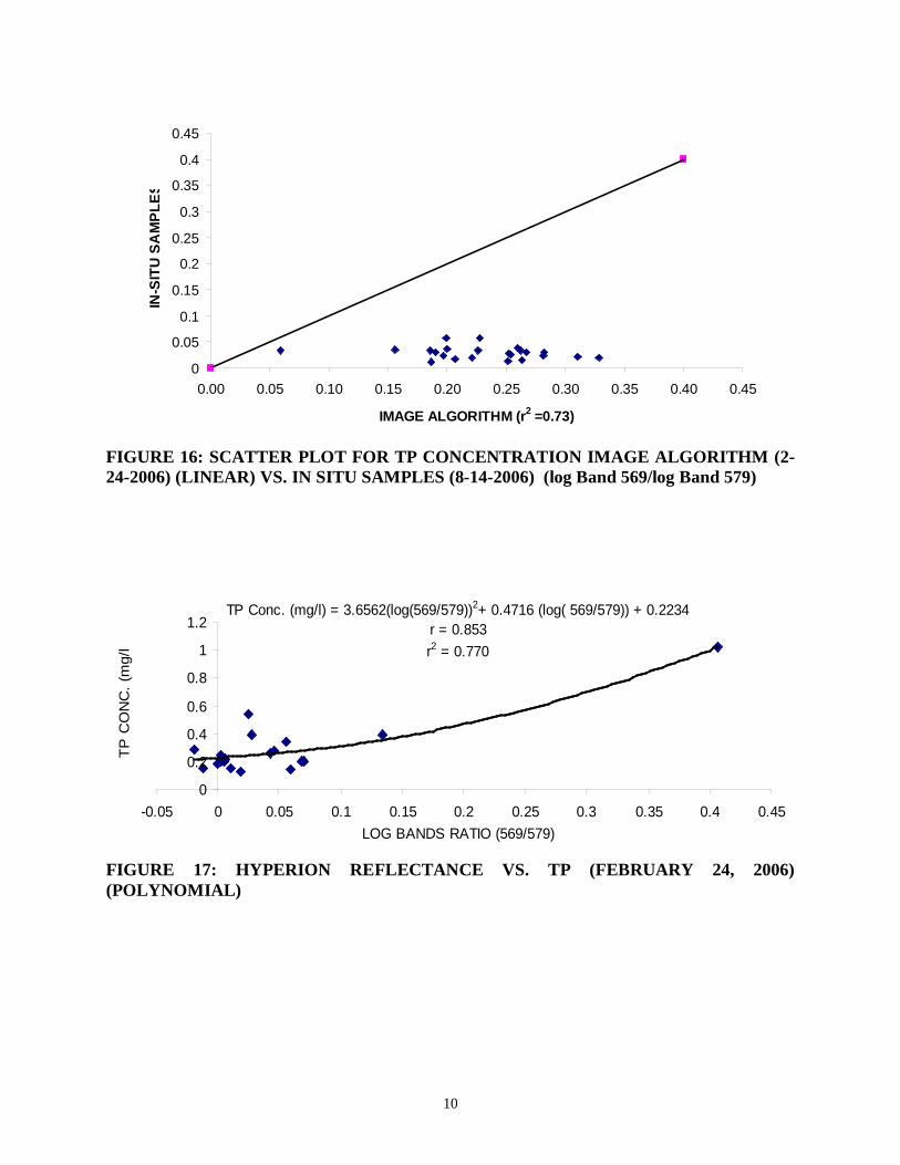
FIGURE 16: SCATTER PLOT FOR TP CONCENTRATION IMAGE ALGORITHM (2-24-2006) (LINEAR) VS. IN SITU SAMPLES (8-14-2006) (log Band 569/log Band 579)

FIGURE 17: HYPERION REFLECTANCE VS. TP (FEBRUARY 24, 2006) (POLYNOMIAL)

TP Conc. (mg/l) = 3.6562(log(569/579))2+ 0.4716 (log( 569/579)) + 0.2234r = 0.853r2 = 0.770

0

0.2

0.4

0.6

0.8

1

1.2

-0.05 0 0.05 0.1 0.15 0.2 0.25 0.3 0.35 0.4 0.45LOG BANDS RATIO (569/579)

TP C

ON

C. (

mg/

l

11

0.0000.0500.1000.1500.2000.2500.3000.3500.4000.4500.500

266

268

269

270

271

272

276

277

280

281

282

283

284

286

287

288

292

294

295

296

298

299

300

301

302

304

305

STATION NUMBER

TP C

ON

C. (

mg/

FIGURE 18: HYPERION REFLECTANCE VS. TP (FEBRUARY 24, 2006) (POLYNOMIAL) ALGORITHM VALIDATION WITH 5-12-2006 IN-SITU SAMPLES

0

0.1

0.2

0.3

0.4

0.5

0.6

0.0 0.1 0.2 0.3 0.4 0.5 0.6


IN-S

ITU

SAM

PLES

FIGURE 19: SCATTER PLOT FOR TP CONCENTRATION IMAGE ALGORITHM (2-24-2006) (POLYNOMIAL) VS. IN SITU SAMPLES (5-12-2006) (log Band 569/log Band 579)

12

0.000

0.050

0.100

0.150

0.200

0.250

0.300

0.350

0.400

268

269

270

271

273

274

277

278

279

280

281

283

284

287

288

289

290

292

293

295

299

303

305

TP C

ONC

. (m

g/l

STATION NUMBER

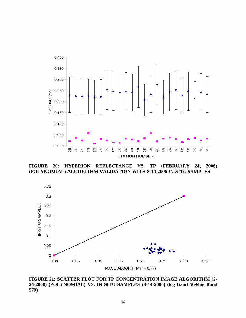
FIGURE 20: HYPERION REFLECTANCE VS. TP (FEBRUARY 24, 2006) (POLYNOMIAL) ALGORITHM VALIDATION WITH 8-14-2006 IN-SITU SAMPLES

0

0.05

0.1

0.15

0.2

0.25

0.3

0.35

0.00 0.05 0.10 0.15 0.20 0.25 0.30 0.35

IMAGE ALGORITHM r2 = 0.77)

IN-S

ITU

SA

MP

LES

FIGURE 21: SCATTER PLOT FOR TP CONCENTRATION IMAGE ALGORITHM (2-24-2006) (POLYNOMIAL) VS. IN SITU SAMPLES (8-14-2006) (log Band 569/log Band 579)

13

FIGURE 22: HYPERION REFLECTANCE VS. TP (MAY 12, 2006)

FIGURE 23: HYPERION REFLECTANCE VS. TP (AUGUST 14, 2006)

No validation was completed for the May 12, 2006 and August 14, 2006 individual bands due to their low co-relation coefficient as compared to other bands and band combination regression analyses.

TP CONC (mg/l) = 2.6555* log(772/569) + 0.077

r = 0.59r2 = 0.348

00.10.20.30.40.5

-0.04 -0.02 0 0.02 0.04 0.06 0.08 0.1

LOG BANDS RATIO (Band 772/Band 569)

TP C

ON

C (m

g/l

TP CONC (mg/l) = 0.0665*(600/590) - 0.0321r = 0.565

r2 = 0.3197

0

0.01

0.02

0.03

0.04

0.05

0.06

0 0.2 0.4 0.6 0.8 1 1.2

REFLECTANCE BANDS RATIO

TP C

ONC

(mg/

l

14

TP Conc. (mg/l) = 0.001(396/752)2 + 0.005(396/752) + 0.2265r = 0.625

r2 = 0.4203

0

0.2

0.4

0.6

0.8

1

1.2

-10 -5 0 5 10 15 20 25 30

BAND RATIO (396/752)

TP C

ON

C. (

mg/

l)

FIGURE 24: HYPERION REFLECTANCE VS. TP (FEBRUARY 24, 2006 AND MAY 12, 2006)

0.000

0.050

0.100

0.150

0.200

0.250

0.300

0.350

0.400

268

269

270

271

273

274

277

278

279

280

281

283

284

287

288

289

290

292

293

295

299

303

305

STATION NUMBER

TP C

ON

C. (

mg/

l

FIGURE 25: HYPERION REFLECTANCE VS. TP (FEBRUARY 24, 2006 AND MAY 12, 2006) ALGORITHM VALIDATION WITH 8-14-2006 IN-SITU SAMPLES

15

0

0.05

0.1

0.15

0.2

0.25

0.3

0.00 0.05 0.10 0.15 0.20 0.25 0.30


IN-S

ITU

SAM

PLES

FIGURE 26: SCATTER PLOT FOR TP CONCENTRATION IMAGE ALGORITHM (2-24-2006 and 5-12-2006) VS. IN SITU SAMPLES (8-14-2006) (Band 396/Band 752)

TP Conc. (mg/l) = 0.1741(641/488)2 - 0.1771(641/488) + 0.0683r = 0.565

r2 = 0.4373

0

0.05

0.1

0.15

0.2

0.25

0.3

0 0.2 0.4 0.6 0.8 1 1.2 1.4 1.6


TP C

ON

C. (

mg/

FIGURE 27: HYPERION REFLECTANCE VS. TP (MAY 12, 2006 AND AUGUST 14, 2006)

16

0.0000.1000.2000.3000.4000.5000.6000.7000.8000.9001.000

269

271

272

273

274

276

281

282

283

284

286

287

288

291

292

293

296

297

298

299

300

301

STATION NUMBER

TP C

ON

C. (

mg/

FIGURE 28: HYPERION REFLECTANCE VS. TP (MAY 12, 2006 AND AUGUST 14, 2006) ALGORITHM VALIDATION WITH 2-24-2006 IN-SITU SAMPLES

0

0.2

0.4

0.6

0.8

1

1.2

0.0 0.2 0.4 0.6 0.8 1.0 1.2


IN-S

ITU

SA

MP

LES


17

TP Conc. (mg/l) = 0.0065exp(2.3736(band 457/band 529))r = 0.731

r2 = 0.8364

00.10.20.30.40.50.60.70.80.9

1

0 0.2 0.4 0.6 0.8 1 1.2 1.4 1.6 1.8 2BAND RATIO (457/529)

TP C

ON

C. (

mg/

l

FIGURE 30: HYPERION REFLECTANCE VS. TP (FEBRUARY 24, 2006 AND AUGUST 14, 2006) (Band 457/Band529)

0.000

0.100

0.200

0.300

0.400

0.500

0.600

0.700

266

268

269

270

271

272

276

277

280

281

282

283

284

286

287

288

292

294

295

296

298

299

300

301

302

304

305

STATION NUMBER

TP C

ON

C. (

mg/

l

FIGURE 31: HYPERION REFLECTANCE VS. TP (FEBRUARY 24, 2006 AND AUGUST 14, 2006) ALGORITHM VALIDATION WITH 5-12- 2006 IN-SITU SAMPLES (Band 457/Band 529)

18

0

0.1

0.2

0.3

0.4

0.5

0.6

0.0 0.1 0.2 0.3 0.4 0.5 0.6


IN-S

ITU

SA

MP

LE


TP Conc. (mg/l) = 0.0139exp(2.6838(428/529))r = 0.720 r2 = 0.830

0

0.1

0.2

0.3

0.4

0.5

0.6

0.7

0.8

0.9

1

0 0.2 0.4 0.6 0.8 1 1.2 1.4 1.6


TP C

ON

C. (

mg/

FIGURE 33: HYPERION REFLECTANCE VS. TP (FEBRUARY 24, 2006 AND AUGUST 14, 2006) (Band 428/Band529)

19

0.000

0.100

0.200

0.300

0.400

0.500

0.600

0.700

266

268

269

270

271

272

276

277

280

281

282

283

284

286

287

288

292

294

295

296

298

299

300

301

302

304

305

STATION NUMBER

TP C

ON

C. (

mg/

l

FIGURE 34: HYPERION REFLECTANCE VS. TP (FEBRUARY 24, 2006 AND AUGUST 14, 2006) ALGORITHM VALIDATION WITH 5-12- 2006 IN-SITU SAMPLES (Band 428/Band 529)

0

0.1

0.2

0.3

0.4

0.5

0.6

0.0 0.1 0.2 0.3 0.4 0.5 0.6


IN-S

ITU

SA

MP

LES


20

TP Conc. (mg/l) = 0.0003exp(4.7341(488/529))r = 0.750

r2 = 0.7652

00.10.20.30.40.50.60.70.80.9

1

0 0.2 0.4 0.6 0.8 1 1.2 1.4 1.6


TP C

ON

C. (

mg/

l

FIGURE 36: HYPERION REFLECTANCE VS. TP (FEBRUARY 24, 2006 AND AUGUST 14, 2006) (Band 488/Band 529)

0.000

0.100

0.200

0.300

0.400

0.500

0.600

0.700

266

268

269

270

271

272

276

277

280

281

282

283

284

286

287

288

292

294

295

296

298

299

300

301

302

304

305

STATION NUMBER

TP C

ON

C. (

mg/

l

FIGURE 37: HYPERION REFLECTANCE VS. TP (FEBRUARY 24, 2006 AND AUGUST 14, 2006) ALGORITHM VALIDATION WITH 5-12- 2006 IN-SITU SAMPLES (Band 488/529)

21

0

0.1

0.2

0.3

0.4

0.5

0.6

0.0 0.1 0.2 0.3 0.4 0.5 0.6


IN-S

ITU

SAM

PLE


TP Conc. (mg/l) = 0.0425exp(12.175 log(Band 488/Band 529))r = 0.719

r2 = 0.7391

-0.15 -0.1 -0.05 0 0.05 0.1 0.15 0.2

LOG BANDS RATIO (488/529)

TP C

ON

C. (

mg/

FIGURE 39: HYPERION REFLECTANCE VS. TP (FEBRUARY 24, 2006 AND AUGUST 14, 2006) (log Band 488/log Band 529)

22

0.000

0.100

0.200

0.300

0.400

0.500

0.600

0.700

266

268

269

270

271

272

276

277

280

281

282

283

284

286

287

288

292

294

295

296

298

299

300

301

302

304

305

STATION NUMBER

TP C

ON

C. (

mg/

l

FIGURE 40: HYPERION REFLECTANCE VS. TP (FEBRUARY 24, 2006 AND AUGUST 14, 2006) ALGORITHM VALIDATION WITH 5-12- 2006 IN-SITU SAMPLES (log Band 488/log Band 529)

FIGURE 41: SCATTER PLOT FOR TP CONCENTRATION IMAGE ALGORITHM VS. IN SITU SAMPLES (log Band 488/log Band 529)

23

TP = 0.0425exp(-12.175(log bands(529/488)))r = 0.720

r2 = 0.7391

-0.2 -0.15 -0.1 -0.05 0 0.05 0.1 0.15

LOG BAND RATIO (529/488)

TP C

onc.

(mg/

l

FIGURE 42: HYPERION REFLECTANCE VS. TP (FEBRUARY 24, 2006 AND AUGUST 14, 2006) (log Band 529/log Band 488)

0.000

0.100

0.200

0.300

0.400

0.500

0.600

0.700

266

268

269

270

271

272

276

277

280

281

282

283

284

286

287

288

292

294

295

296

298

299

300

301

302

304

305

STATION NUMBER

TP C

ON

C. (

mg/

l

FIGURE 43: HYPERION REFLECTANCE VS. TP (FEBRUARY 24, 2006 AND AUGUST 14, 2006) ALGORITHM VALIDATION WITH 5-12- 2006 IN-SITU SAMPLES (log Band 529/log Band 488)

24

FIGURE 44: SCATTER PLOT FOR TP CONCENTRATION IMAGE ALGORITHM VS. IN SITU SAMPLES (log Band 529/log Band 488)

TP Conc. (mg/l) = 0.025exp(1.5027(Band 457/Band 529))r = 0.527

r2 = 0.3572

00.1

0.20.30.40.5

0.60.70.8

0.91

0 0.2 0.4 0.6 0.8 1 1.2 1.4 1.6 1.8 2BAND RATIO (457/529)

TP C

ON

C. (

mg/

l

FIGURE 45: HYPERION REFLECTANCE VS. TP CONCENTRATIONS (FEBRUARY 24, MAY 12, AND AUGUST 14, 2006) (Band 457/Band 529)

25

Table 1 shows the estimated statistical errors for individual bands and combinations producing the higher co-relations.

TABLE 1- STATISTICAL ERRORS REGRESSION

ANALYSES BAND

COMB. ME RE (%) AME RMS VARIANCE

2/24/2006- Algorithm with 5/12/2006 (Linear)

770/778 -0.913 4.06 0.913 0.949 0.246


LOG (569/579)

-0.062 1.68 0.017 0.132 0.008

2/24/2006- Algorithm with 5/12/2006 (Polynomial)

LOG (569/579)

-0.170 25.40 0.170 0.209 0.012

2/24/2006 and 5/12/2006-Algorithm with 8/14/2006 (Polynomial)

396/752 -0.171 25.52 0.171 0.186 0.01

5/12/2006 and 8/14/2006- Algorithm with 2/24/2006 (Polynomial)

641/488 0.192 2.46 0.201 0.366 0.05

2/24/2006 and 8/14/2006- Algorithm with 5/12/2006 (Exponential)

428/529 0.110 2.47 0.110 0.160 0.01


457/529 0.110 2.73 0.110 0.154 0.009


488/529 0.113 3.08 0.113 0.162 0.01


LOG (488/529) 0.106 1.03 0.106 0.158 0.01


LOG (529/488) 0.106 2.91 0.106 0.158 0.01

where: ME = Mean error AME = Absolute Mean Error RMS = Root Mean Square Error RE = Relative Error Table 2 shows the uncertainty analyses, estimated by the safety margin method, also completed for individual bands and combinations.

26

TABLE 2- UNCERTAINTY ANALYSIS

REGRESSION ANALYSES

BAND COMB. SMµ COV 2

SMσ SMσ α CERT. PROB.


LOG (569/579) 0.054 0.00002 0.014 0.118 0.462 0.6771

2/24/2006 and 5/12/2006-Algorithm with 8/14/2006 (Polynomial) 396/752 -0198 -0.00467 0.023 0.152 -1.30 0.097

2/24/2006 and 8/14/2006- Algorithm with 5/12/2006 (Exponential) 428/529 0.054 0.00002 0.014 0.118 0.462 0.6771

2/24/2006 and 8/14/2006- Algorithm with 5/12/2006 (Exponential) 457/529 0.045 -0.00009 0.014 0.119 0.38 0.6509

2/24/2006 and 8/14/2006- Algorithm with 5/12/2006 (Exponential) 488/529 0.057 -0.000095 0.014 0.119 0.48 0.6843


LOG (488/529) 0.051 -0.000109 0.014 0.119 0.42 0.6626


LOG (529/488)

0.051 -0.000109 0.014 0.119 0.42 0.6626

where: CERT. PROB. = certainty probability µ = mean value of xi and yi

µsm = mean value safety and margin =SMσ standard deviation safety and margin

=2SMσ variance of xi and yi safety and margin

Cov = covariance of random variables Based on the above evaluations, the selected algorithm corresponded to the log bands ratio vs. total phosphorus concentration for the February 24, 2006 and August 14, 2006 combined reflectance data and validated with the May 12, 2006 TP in-situ samples results. That data showed a correlation coefficient of 0.74. The exponential model is defined by the following empirical algorithm:

27

TP Concentration (mg/l) = 0.0425*exp(12.175*log(Band 488/Band 529))

The reflectance values of the Hyperion image collected during February 24, May 12, and August 14, 2006 were changed to total phosphorus concentration by applying the above algorithm, which resulted in three new images. The resulting images are shown as Figures 29, 30, and 31.

Figure 29

February 24, 2006

Figure 30

May 12, 2006

28

Figure 30

August 14, 2006

The results of this study show that hyperspectral remote sensing technology is of significant potential use for the water quality management of such impaired surface waters. The following conclusions are emphasized. • Based on the image results the SJL is heavily polluted with TP where the water quality

standard is exceeded in at least five times its maximum value of 0.1 parts per million. • Hyperspectral remote sensing is an economically feasible tool for the monitoring of total

phosphorus in a eutrophic tropical lagoon. • The FLAASH atmospheric correction algorithm better adapts to the Hyperion image

processing than ACORN when evaluating eutrophic water systems. • The 1995 COE’s calibrated hydrodynamic model shows TP results consistent with the

February 24, 2006 Hyperion image, after transformed with the empirical algorithm. This is evidenced by the similar results shown by the model and Hyperion where significantly higher TP concentrations (over 0.5 parts per million) are produced within the dredged pits locations and at the Martín Peña inlet to the lagoon. Based on these results it can be inferred that:

o No significant changes have occurred to Caño Martín Pena or Suárez Channel in the

intervening years. This means that the flows in/out of the San José Lagoon are essentially the same in 2006 as 1995.

o No significant changes in watershed directly contributing to the SJL. It was a fully developed watershed in 1995. The infrastructure is essentially unchanged in the watershed so the volume of and loads in the runoff are comparable.

o Hydrodynamic and water quality information had been already been observed for 1995. It is unlikely to find as extensive a water quality data set in other years as compared to 1995. Any uncertainty induced using an incomplete data set for another year is as large, or larger than the uncertainty induced comparing 2006 and 1995.

o No significant changes to the bathymetry of the lagoon, (i.e., no significant dredging or filling). This means that the hydraulic residence time is "unchanged" and the sediment/water column processes associated with the existing dredge holes are unchanged.

29

• The correlation analysis completed between the spectral characteristics obtained and the TP suggests the possibility of accurately mapping the TP concentration in a surface water system.

• Log band ratios provide stronger co-relations between Hyperion reflectance values and TP concentrations (within the 428-529 nm range of the visible region of the spectrum) in eutrophic water systems.

• Band ratios provide better co-relations between field spectrometer reflectance results and TP concentrations (within the 770-780 nm range within the near infra-red region of the spectrum) in eutrophic water systems.

The following recommendation should be considered for further studies and research:

• The use of hyperspectral remote sensing technology may be a useful to establish and implement TP as point and non-point source pollution control strategies (i.e., Total Maximum Daily Loads, Waste Load Allocations, Assimilative Capacity Studies) in eutrophic surface waters and watersheds. Its use in larger surface water systems may be centered on the calibration and validation of water quality models based on the TP spectral characteristics.

Some of the limitations of the hyperspectral remote sensing technology applicability in the SJL may be summarized as follows:

• While the Hyperion high spectral resolution is responsible for the definition of the TP reflectance characteristics its applicability to smaller surface water systems may not result to be the best alternative due to its lower spatial accuracy.

• The use of remote sensing in shallow turbid waters requires additional spectral corrections, through modeling, due to the reflectance misleading effect caused by the bottom.

• The Hyperion’s low signal-to-noise ratio in several spectral bands provides for its low reflectance responsiveness producing negative reflectance values in the blue (400-500 nm) and infrared (800-1200 nm) regions.

PUBLICATIONS

No publications were completed during the year as a result of work funded under Section 104 during the current budget period.

30

TRAINING ACCOMPLISMENTS List all students participating in Section 104 projects.

Field of study Academic Level Total Undergraduate MS Ph.D. Post

Ph.D. Chemistry Engineering:

Agricultural Civil 1 1

Chemistry Computer Electrical Industrial

Mechanical Geology Hydrology Agronomy Biology Ecology Fisheries, Wildlife, and Forestry

Computer Science Economics Geography Law Resources Planning Social Sciences Business Administration Other (specify)

Totals 1

Monitoring Phosphorus Content in a Tropical Estuary …gers.uprm.edu/pdfs/report_sjbay.pdf1...

Documents

Transcript of Monitoring Phosphorus Content in a Tropical Estuary …gers.uprm.edu/pdfs/report_sjbay.pdf1...