MONITORING PARTICLE IMPACT ENERGY USING ACOUSTIC …

MONITORING PARTICLE IMPACT ENERGY USING

ACOUSTIC EMISSION TECHNIQUE

Mohamad Ghazi Droubi

A dissertation submitted for the degree of Doctor of Philosophy

Heriot-Watt University

School of Engineering and Physical Sciences

April 2013

This copy of the thesis has been supplied on condition that anyone who consults it is

understood to recognise that the copyright rests with its author and that no quotation

from the thesis and no information derived from it may be published without the prior

written consent of the author or of the University (as may be appropriate).

ACADEMIC REGISTRY

Research Thesis Submission

Name: Mohamad Ghazi Droubi

School/PGI: School of Engineering and Physical Sciences

Version: (i.e. First,

Resubmission,

Final)

Final Degree Sought

(Award and

Subject area)

PhD Mechanical Engineering

Declaration

In accordance with the appropriate regulations I hereby submit my thesis and I declare that:

1) the thesis embodies the results of my own work and has been composed by myself

2) where appropriate, I have made acknowledgement of the work of others and have made reference

to work carried out in collaboration with other persons

3) the thesis is the correct version of the thesis for submission and is the same version as any

electronic versions submitted*.

4) my thesis for the award referred to, deposited in the Heriot-Watt University Library, should be

made available for loan or photocopying and be available via the Institutional Repository, subject

to such conditions as the Librarian may require

5) I understand that as a student of the University I am required to abide by the Regulations of the

University and to conform to its discipline.

* Please note that it is the responsibility of the candidate to ensure that the correct version of the

thesis is submitted.

Signature of

Candidate:

Date:

Submission

Submitted By (name in capitals):

Signature of Individual Submitting:

Date Submitted:

For Completion in Academic Registry

Received in the Academic Registry

by (name in capitals):

Method of Submission

(Handed in to Academic Registry;

posted through internal/external

mail):

E-thesis Submitted (mandatory for

final theses from January 2009)

Signature:

Date:

iii

Abstract

The estimation of energy dissipated during multiple particle impact is a key aspect in

evaluating the abrasive potential of particle-laden streams. A systematic investigation of

particle impact energy using acoustic emission (AE) measurements is presented in this

thesis with experiments carried out over a range of particle sizes, particle densities and

configurations. A model of the AE impact time series is developed and validated on

sparse streams where there are few particle overlaps and good control over particle

kinetic energies. The approach is shown to be robust and extensible to cases where the

individual particle energies cannot be distinguished.

For airborne particles, a series of impact tests was carried out over a wide range of

particle sizes (from 125 microns to 1500 microns) and incident velocities (from 0.9 ms-1

to 16 ms-1

). Two parameters, particle diameter and particle impact speed, both of which

affect the energy dissipated into the material, were investigated and correlated with AE

energy. The results show that AE increases with the third power of particle diameter, i.e.

the mass, and with the second power of the velocity, as would be expected. The

diameter exponent was only valid up to particle sizes of around 1.5mm, an observation

which was attributed to different energy dissipation mechanisms with the higher

associated momentum. The velocity exponent, and the general level of the energy were

lower for multiple impacts than for single impacts, and this was attributed to particle

interactions in the guide tube and/or near the surface leading to an underestimate of the

actual impact velocity in magnitude and direction.

In order to develop a model of the stream as the cumulation of individual particle arrival

events, the probability distribution of particle impact energy was obtained for a range of

particle sizes and impact velocities. Two methods of time series processing were

investigated to isolate the individual particles arrivals from the background noise and

from particle noise associated with contact of the particles with the target after their first

arrival. For the conditions where it was possible to resolve individual impacts, the

probability distribution of particle arrival AE energy was determined by the best-fit

lognormal probability distribution function. The mean and variance of this function was

then calibrated against the known nominal mass and impact speed. A pulse shape

function was devised for the target plate by inspection of the records, backed up by

pencil lead tests and this, coupled with the energy distribution functions allowed the

iv

records to be simulated knowing the arrival rate and the nominal mass and velocity of

the particles. A comparison of the AE energy between the recorded and simulated

records showed that the principle of accumulating individual particle impact signatures

could be applied to records even when the individual impacts could not be resolved.

For particle-laden liquid, a second series of experiments was carried out to investigate

the influence of particle size, free stream velocity, particle impact angle, and nominal

particle concentration on the amount of energy dissipated in the target using both a

slurry impingement erosion test rig and a flow loop test rig. As with airborne particles,

the measured AE energy was found overall to be proportional to the incident kinetic

energy of the particles. The high arrival rate involved in a slurry jet or real industrial

flows poses challenges in resolving individual particle impact signatures in the AE

record, hence, and so the model has been further developed and modified (extended) to

account for different particle carrier-fluids and to situations where arrivals cannot

necessarily be resolved. In combining the fluid mechanics of particles suspended in

liquid and the model, this model of AE energy can be used as a semi-quantitative

diagnostic indicator for particle impingement in industrial equipments such as pipe

bends.

v

Dedication

I dedicate this work to:

The martyrs of the Syrian

revolution

vi

Acknowledgements

This journey would never have begun, or for that matter reached its end, if it was not for

the generosity and help of ALLAH, then many organizations and individuals along the

way.

All praises and thanks are due to Almighty Allah for providing me this opportunity to

complete this work. Acknowledgement is due to Aleppo University, Technical

Engineering School for granting me the Research Assistantship to pursue my graduate

studies. I express my profound gratitude to Heriot–Watt University, school of

Mechanical and Chemical Engineering for providing me with a decent environment to

carry out my research.

I would like to express my sincere thanks and gratitude to my thesis supervisors,

Professor R L (Bob) Reuben for his valuable supervision, inspiration, constructive

suggestions, constant help and guidance throughout the entire period of my research,

Professor Graeme White for his valuable comments and helpful discussions. I consider

them as my mentors and will continue to seek their guidance in the future.

I am also grateful to all mechanical and electrical technicians in the school of

Engineering and Physical Science for their help in designing, manufacturing, running

and maintaining all my experimental apparatuses. Thanks are also due to my colleagues,

past and present, who made my time very memorable and extremely enjoyable, in

particular, Dr. Mohamad El-Shaib, Dr. Faissal, Dr. Angus, Wael, and Dr. Mansour.

Special thanks for all members of the Syrian community (Together For Syria) for their

wonderful company throughout the course of my research. Special gratitude goes to

Monkiz, Ali, Manhal, and Hassan for motivating me to complete the research with their

unlimited support and love.

Finally and most importantly, I am grateful to my parents and all my family members

for their constant prayers and support, to my loving wife Ruan…. For your love,

support, patience, resilience, and forgiveness, no words will ever express the true extent

of my appreciation, to my small angel Sedra…. Who shared this journey with us and

beard all my stressful moments.

vii

Table of contents

Abstract ................................................................................................................................................. iii

Dedication ............................................................................................................................................... v

Acknowledgements ................................................................................................................................ vi

Table of contents .................................................................................................................................. vii

List of Tables .......................................................................................................................................... x

List of Figures ....................................................................................................................................... xii

Nomenclature ....................................................................................................................................... xx

Chapter 1 ......................................................................................................................... 1

Introduction ..................................................................................................................... 1

1.1 Background ............................................................................................................................... 1

1.2 Research methodology and objectives ...................................................................................... 3

1.3 Thesis outline ............................................................................................................................ 3

1.4 Contribution to knowledge ........................................................................................................ 5

Chapter 2 ......................................................................................................................... 6

Literature review ............................................................................................................. 6

2.1 Impact dynamics and elastic waves........................................................................................... 6

2.1.1 Hertz theory of elastic contact/impact .................................................................................. 6

2.1.2 Elastic plastic contact ......................................................................................................... 10

2.1.3 Contact force-displacement relationships ........................................................................... 14

2.1.4 Coefficient of restitution .................................................................................................... 15

2.1.5 Elastic wave dissipation during contact/impact .................................................................. 17

2.2 Erosive wear of materials ........................................................................................................ 22

2.2.1 Mechanisms of particle erosion .......................................................................................... 22

2.2.2 Erosion testing .................................................................................................................... 27

2.2.3 Empirical observations of factors affecting erosion ........................................................... 32

2.2.4 Erosion models ................................................................................................................... 43

2.2.5 Particle interference effects ................................................................................................ 46

2.2.6 Particle-laden liquids .......................................................................................................... 49

2.3 Acoustic emission technology ................................................................................................. 51

2.3.1 Characteristics of “hit-based” AE ...................................................................................... 52

2.3.2 Application of AE as a tool to monitor erosion damage caused by solid particle impacts . 55

2.4 Identification of thesis topic .................................................................................................... 61

Chapter 3 ....................................................................................................................... 62

Experimental method ................................................................................................... 62

3.1 Materials, instrumentation and signal processing ................................................................... 62

3.1.1 Particle types and target plate details ................................................................................. 62

3.1.2 AE apparatus ...................................................................................................................... 66

3.1.3 AE signal processing techniques ........................................................................................ 69

3.2 Calibration tests ....................................................................................................................... 71

viii

3.2.1 Simulated source for calibration tests ................................................................................. 71

3.2.2 Calibration tests on steel cylinder ....................................................................................... 72

3.2.3 Calibration tests on target ................................................................................................... 74

3.3 Particle impact tests................................................................................................................. 81

3.3.1 Free fall and airborne particle impact tests ......................................................................... 82

3.3.2 Slurry impingement tests .................................................................................................... 90

3.3.3 Flow loop impingement tests.............................................................................................. 96

Chapter 4 ..................................................................................................................... 100

Experimental Results .................................................................................................. 100

4.1 Airborne particle impact test ................................................................................................. 100

4.1.1 Low velocity-low mass impacts ....................................................................................... 100

4.1.2 Low velocity-high mass impacts ...................................................................................... 103

4.1.3 High velocity-low mass impacts ...................................................................................... 105

4.2 Slurry jet impingement test ................................................................................................... 107

4.3 Flow loop test ........................................................................................................................ 118

Chapter 5 ..................................................................................................................... 126

Time series model for particle impacts ..................................................................... 126

5.1 Determination of probability distribution functions .............................................................. 126

5.1.1 Dynamic threshold method............................................................................................... 128

5.1.2 Truncated distribution method ......................................................................................... 131

5.2 Development of time series model ........................................................................................ 133

5.2.1 Correlation between truncated distribution and incident impact energy method using log-

normal distributions ......................................................................................................................... 139

5.2.2 Time series simulation ...................................................................................................... 142

Chapter 6 ..................................................................................................................... 148

Analysis and Discussion .............................................................................................. 148

6.1 Airborne particle impact test ................................................................................................. 148

6.2 Slurry jet impingement .......................................................................................................... 153

6.3 Impacts during pipe flow ...................................................................................................... 159

6.3.1 Analysis for particle-free water ........................................................................................ 160

6.3.2 Slurry impact analysis ...................................................................................................... 170

6.3.3 Application of time series model to flow loop tests ......................................................... 177

Chapter 7 ..................................................................................................................... 182

Conclusions and Recommendations .......................................................................... 182

7.1 Conclusions ........................................................................................................................... 182

7.1.1 Free fall and preliminary airborne particle tests ............................................................... 182

7.1.2 Statistical distribution model ............................................................................................ 183

7.1.3 Slurry jet impingement tests ............................................................................................. 184

7.1.4 Flow loop impingement tests............................................................................................ 185

7.2 Future work ........................................................................................................................... 186

ix

References.........................................................................................................................188

Appendix A..................................................................................................................198

x

List of Tables

Table 3.1: Particle types and sizes used in free-fall and air-assisted experiments for

single and multiple particle impacts. ............................................................................... 63

Table 3.2: Size distribution functions for air-assisted particle impact experiments....... 64

Table 3.3: Particle types and fraction sizes used in slurry impact and flow loop

experiments. .................................................................................................................... 65

Table 3.4: Summary of ANOVA results comparing the effect of demounting the sensor

with the effect of pencil lead breaks at each position ..................................................... 74

Table 3.5: Free-fall particle impact velocity (ms-1

), estimated from Equation 3.2. ....... 85

Table 3.6: Summary of particle and particle stream conditions ..................................... 89

Table 3.7: Summary of measured and derived impingement conditions in slurry impact

rig. ................................................................................................................................... 95

Table 3.8: Summary of derived impingement conditions .............................................. 99

Table 4.1: Exponent of flow speed dependence of measured AE energy for all

experiments. (Data in bold font are plotted in Figures 4.12 and 4.13) ......................... 110

Table 4.2: Exponent of particle size dependence of measured AE energy for all

experiments. (Data in bold font are plotted in Figures 4.14-4.16) ................................ 113

Table 4.3: Exponent of particle concentration dependence of measured AE energy for

all experiments. (Data in bold font are plotted in Figures 4.17 and 4.18) .................... 115

Table 4.4: Power index for sin (nominal impact angle) dependence on the measured AE

energy for all experiments. (Bold text data are shown in Figure 4.19) ......................... 117

Table 4.5: Exponent of flow speed dependence of measured AE energy and correlation

coefficient for all experiments. ..................................................................................... 120

Table 4.6: Exponent of particle size dependence of measured AE energy for all

experiments. .................................................................................................................. 122

Table 4.7: Exponent of particle concentration dependence of measured AE energy for

all experiments. ............................................................................................................. 125

Table 5.1:Derived particle and particle stream conditions. See text for shaded

conditions. ..................................................................................................................... 135

Table 6.1: Calculated particle arrival speed using the model of Turenne and Fiset [94]

....................................................................................................................................... 156

Table 6.2: summary of correlation functions between calculated and measured AE

energy. ........................................................................................................................... 158

xi

Table 6.3: Exponent of flow speed dependence of the static component of measured AE

energy for all flow loop tests. ........................................................................................ 172


....................................................................................................................................... 178

xii

List of Figures

Figure 2.1: Plastic deformation process during the compression of a spherical indenter

into a plastic solid (a) the onset of plastic deformation, (b) expansion of plastic zone

[29] .................................................................................................................................. 12

Figure 2.2: Régime diagram for elastic-plastic contact [27] .......................................... 13

Figure 2.3: The main AE waves in infinite and semi-infinite media [37] ..................... 18

Figure 2.4: Zero-order Lamb wave [37]......................................................................... 19

Figure 2.5: Basic mechanisms of particle erosion [42]. ................................................. 24

Figure 2.6: Impact material removal mechanism for a brittle material [1] .................... 24

Figure 2.7: Impact material removal mechanism for a ductile material [1] ................... 25

Figure 2.8: Modes of deformation, (a) cutting deformation, (b) ploughing deformation

with an angular particle, (c) ploughing deformation with a sphere [7] ........................... 26

Figure 2.9: Centrifugal accelerator type erosion tester [75]........................................... 29

Figure 2.10: The gas-blast type erosion tester [56] ........................................................ 30

Figure 2.11: Pot tester used for conducting wear studies [66] ....................................... 31

Figure 2.12: Schematic view of the jet impingement tester used by Ferrer et al [21] ... 31

Figure 2.13: Effect of impact angle on erosion for brittle and ductile materials [17] .... 33

Figure 2.14: Variation of erosion rate and erosion mechanism of 1017 steel (ductile) as

a function of impingement angle at impact velocity of 15 m/s [49] ............................... 34

Figure 2.15: Variation of erosion rate and erosion mechanism of high-Cr white cast

iron as a function of impingement angle at impact velocity of 15 m/s [49] ................... 35

Figure 2.16: Variation of erosion rate for AA6063 material by a narrow size range of

particles (550 µm) with impact angle at different concentrations [66] ........................... 37

Figure 2.17: Variation of linear wear rate with respect to solid particle size [74] ......... 38

Figure 2.18: Contact area due to impact of spherical and angular particles [67] ........... 40

Figure 2.19: Erosion rate due to particles of different shapes [11] ................................ 41

Figure 2.20: Effect of hardness on erosion rate for a range of ductile and brittle

materials [76] .................................................................................................................. 43

Figure 2.21: Working principle of AE technique [95]. .................................................. 52

Figure 2.22: AE signal wave types [43] ......................................................................... 53

Figure 2.23: Traditional time-based features of AE signals. Adapted from [99]........... 54

Figure 3.1: Measured particle size distribution for glass beads in size range 710-850μm.

......................................................................................................................................... 65

Figure 3.2: Silica sand erodent particles of size fraction 300-425 µm........................... 65

xiii

Figure 3.3: Sectional view of target plate in sample holder ........................................... 66

Figure 3.4: Schematic view of the AE acquisition system ............................................. 66

Figure 3.5: The AE acquisition system .......................................................................... 67

Figure 3.6: (a) Pre-amplifier, (b) Signal conditioning unit, connector block and gain

programmer ..................................................................................................................... 68

Figure 3.7: Steps of demodulation frequency analysis, (a) raw AE signal, (b) RMS of the

AE signal, using averaging time of 0.2 ms ..................................................................... 71

Figure 3.8: Hsu-Nielsen source and guide ring [113] .................................................... 72

Figure 3.9: Sensor calibration set-up (a) schematic view of steel cylinder arrangement,

(b) plan view of sensor positions relative to the cylinder and supports. ......................... 72

Figure 3.10: AE energy recorded at the four calibration positions on the steel cylinder

......................................................................................................................................... 73

Figure 3.11: Recorded AE energy for simulated sources at four positions (results of five

independent tests between which the sensor was removed and replaced) ...................... 74

Figure 3.13: Recorded AE energy for simulated sources across the target diameter

(results of two independent experiments between which the sensor was removed and

replaced) .......................................................................................................................... 75

Figure 3.12: Schematic view of the target calibration arrangement. ............................ 75

Figure 3.14: Testing of repeatability of recorded AE energy using H-N source ........... 76

Figure 3.15: Typical raw AE signal for a pencil lead break on the face of the target

plate: (a) a full record, (b) a magnified view of (a) ......................................................... 77

Figure 3.16: Typical raw AE signal for a pencil lead break on the face of the steel

cylinder: (a) a full record, (b) a magnified view of (a), (c) a magnified view of (b) ...... 78

Figure 3.17: AE energy for a pencil lead break on the face of the target plate and on the

face of the steel cylinder ................................................................................................. 79

Figure 3.18: AE decay time for a pencil lead break on the face of the target plate and on

the face of the steel cylinder............................................................................................ 79

Figure 3.19: Typical raw AE frequency domain for a pencil lead break: (a) on the face

of the target plate, (b) on the face of the steel cylinder ................................................... 81

Figure 3.20: Free fall impingement arrangements: (a) individual large particles, (b)

individual small particles using vibrating ramp, (c) multiple small particles. ................ 83

Figure 3.21: Air-assisted particle impact test arrangement ............................................ 86

Figure 3.22: Variation of particle velocity with nozzle pressure drop for two particle

size ranges. ...................................................................................................................... 87

Figure 3.23: Dependence of particle velocity on air speed and particle diameter ......... 88

xiv

Figure 3.24: Schematic diagram of slurry impingement rig. ......................................... 90

Figure 3.25: Tee joint inside the tank used for mixing .................................................. 91

Figure 3.26: Two views of target plate and sensor arrangement for slurry impingement

tests. ................................................................................................................................. 92

Figure 3.27: Two views for the specimen holder position inside the tank. ................... 93

Figure 3.28: Recorded AE energy for pure water jet impingement in slurry impact rig 94

Figure 3.29: Sketch of the experimental flow loop with AE measurement system ....... 96

Figure 3.30: Sectional view of carbon steel bend test section ....................................... 97

Figure 3.31: Recorded AE energy for pure water impingement in flow loop ............... 98

Figure 4.1: AE energy per unit mass of particle versus particle velocity for low velocity

– low mass individual impacts. ..................................................................................... 101

Figure 4.2: AE energy per unit velocity versus mean particle diameter for low velocity

– low mass individual impacts ...................................................................................... 101

Figure 4.3: AE energy per particle per unit mass versus particle velocity for low

velocity – low mass particle streams ............................................................................. 102

Figure 4.4: AE energy per particle per unit velocity versus mean particle diameter for

low speed – low mass particle streams ......................................................................... 103

Figure 4.5: AE energy per unit mass of particle versus particle velocity for low velocity

– high mass individual impacts ..................................................................................... 104

Figure 4.6: AE energy per unit velocity of particle versus particle diameter for low

velocity – high mass individual impacts ....................................................................... 104

Figure 4.7: AE energy per unit mass of particle versus particle velocity for high

velocity – low mass single impacts ............................................................................... 105

Figure 4.8: AE energy per unit velocity versus particle diameter for high velocity – low

mass single impacts ....................................................................................................... 106

Figure 4.9: AE energy per particle per unit mass versus particle velocity for high

velocity – low mass multiple impacts ........................................................................... 106

Figure 4.10: AE energy per particle per unit velocity versus diameter for high velocity

– low mass multiple impacts ......................................................................................... 107

Figure 4.11: Typical 1-second AE records for (a) water and (b) slurry with 300-425 µm

sand, at (i) a flow speed of 4.2m/s and a nominal particle concentration of 10kg/m3 and

(ii) a flow speed of 12.7m/s and a nominal particle concentration of 50kg/m3 Graphs (c)

show the RMS AE signal magnified to reveal events, with record c(i) corresponding to

around 70 particle launches and record c(ii) corresponding to around 1000 particle

launches. ........................................................................................................................ 108

xv

Figure 4.12: Effect of flow speed on AE energy for the three particle sizes at a

concentration of 5kg/m3 impinging at normal incidence. ............................................. 109

Figure 4.13: Effect of flow speed on AE energy for the three concentrations for

particles in size range 125-180 µm impinging at normal incidence ............................. 110

Figure 4.14: Effect of mean particle diameter on AE energy for normal impact at the

four nozzle exit velocities with a 1% slurry. ................................................................. 111


four nozzle exit velocities with a 2.5% slurry. .............................................................. 112


four nozzle exit velocities with a 5% slurry. ................................................................. 112

Figure 4.17: Effect of nominal solid concentration AE energy for normal incidence for

the smaller particle sizes. .............................................................................................. 114

Figure 4.18: Effect of nominal solid concentration AE energy for normal incidence for

the smaller particle sizes. .............................................................................................. 114

Figure 4.19: The effect of the sine of the impact angle on AE energy, for a 5% slurry

....................................................................................................................................... 116

Figure 4.20: Effect of flow speed on the measured AE energy for the three

concentrations for particle size range 212-250 µm ....................................................... 118







Figure 4.24: Effect of mean particle diameter on the measured AE energy at the four

flow speeds with a 1% slurry. ....................................................................................... 121


flow speeds with a 2.5% slurry. .................................................................................... 121


flow speeds with a 5% slurry. ....................................................................................... 122

Figure 4.27: Effect of nominal solid concentration on the measured AE energy for the

four flow speeds for particle size range 212-250 µm .................................................... 123



xvi





Figure 5.1: Typical 5-second record for particle impacts: (a) raw AE signal, (b) RMS AE

signal. 710-850 μm glass beads, impact velocity 10.1 ms-1

. ......................................... 128

Figure 5.2: Magnified view of (a) raw and (b) RMS AE signal shown in Figure 5.1,

illustrating dynamic threshold method. ......................................................................... 129

Figure 5.3: Distribution of AE energy attributed to particle impact from record shown

in Figure 5.1 using dynamic threshold approach. ......................................................... 130

Figure 5.4: Probability function fit to distribution of AE energy attributed to particle

impact from record shown in Figure 5.1 using the dynamic threshold approach: (a)

bimodal distribution and (b) log-normal distribution................................................... 131

Figure 5.5: Magnified view of (a) raw and (b) RMS AE signal shown in Figure 5.1,

illustrating truncated distribution method. .................................................................... 132

Figure 5.6: Probability function fit to distribution of AE energy attributed to particle

impact from record shown in Figure 5.1 using the truncated distribution approach. (a)

bimodal distribution and (b) log-normal distribution.................................................... 133

Figure 5.7: Expected distribution of incident particle energy, accounting for particle

size distribution only. .................................................................................................... 134

Figure 5.8: Values of fraction of particles colliding derived from the simulations of

Gomes-Ferreira et al [84]. Dotted and chained lines are manual extrapolations of the

simulation results to low particle densities. .................................................................. 136

Figure 5.9: Dependence of comparative error upon average particle arrival rate using

the dynamic threshold method for the particle size range 850μm to 300 μm. .............. 137


the truncated energy method for the particle size range 850μm to 212 μm. ................. 138


the truncated energy method for the particle size range 850μm to 300 μm. ................. 138

Figure 5.12: Correlation between the mean of the log-normal distribution and nominal

incident energy. ............................................................................................................. 139

Figure 5.13: Correlation between the variance of the log-normal distribution and

nominal incident energy. ............................................................................................... 140

Figure 5.14: Correlation of mean distribution AE energy with mean AE energy for

single impacts. ............................................................................................................... 140

xvii

Figure 5.15: Truncated energy versus particle impact speed. ...................................... 141

Figure 5.16: Raw AE signal for pencil lead break on the face of the sample. The pulse

shape is identified by the solid lines bounding the signal. ............................................ 143

Figure 5.17: Raw AE signal for pencil lead break on the face of a large cylindrical steel

block. Curve (a) is the decay curve estimated from Ivantsiv et al [102], and Curve (b) is

the decay curve for the target plate. .............................................................................. 144

Figure 5.18: Measured (top) and simulated AE records for 212-250μm silica sand with

nominal impact velocity of 12.3 ms-1

, and particle arrival rate of 900 per second. Peaks

that were identified as particle impacts in the measured record are labelled. ............... 145

Figure 5.19: Measured (top) and simulated AE records for 710-850μm glass beads with

nominal impact velocity of 4 ms-1

, and particle arrival rate of 40 per second. Peaks that

were identified as particle impacts in the measured record are labelled. ...................... 146

Figure 5.20: Measured (top) and simulated AE records for 125-180 μm silica sand with


, and particle arrival rate of 4000 per second

Simulations with a decay constant of 3000sec-1

(middle) and 30000sec-1

(lower) ...... 146

Figure 5.21: AE energy from simulated time series signal versus raw AE energy ...... 147

Figure 6.1: AE energy per unit mass versus particle velocity for all regimes

investigated: (A) low velocity, (5) high velocity-low mass single impacts, (6) high

velocity-low mass multiple impacts .............................................................................. 149

Figure 6.2: AE energy per unit mass versus particle velocity for all low velocity

measurements (area A above): (1a) low mass-lower range single impacts, (1b) low

mass-higher range single impacts, (2) low mass multiple impacts, (3) high mass-lower

range, (4) high mass-higher range ................................................................................. 149

Figure 6.3: AE energy per particle divided by the square of the velocity versus particle

diameter for all regimes investigated: (B) low velocity-low mass regime, (3) high mass-

lower range, (4) high mass-higher range, (5) high velocity-low mass single impacts, (6)

high velocity-low mass multiple impacts ...................................................................... 150

Figure 6.4: AE energy per particle divided by the square of the velocity versus particle

diameter for low velocity-low mass regime (area B above): (1) low velocity-low mass

single impacts, (2) low velocity-low mass multiple impacts ........................................ 151

Figure 6.5: The dependence of AE energy per unit mass upon particle velocity ........ 152

Figure 6.6: Influence of mean particle diameter on AE energy divided by the square of

impact velocity .............................................................................................................. 153

Figure 6.7: Correlation between the mean of the lognormal distribution and nominal

incident energy, using data from Figure 5.12. .............................................................. 154

xviii

Figure 6.8: Measured and calculated AE energy, assuming the particle arrival speeds

given in Table 3.7. ......................................................................................................... 155

Figure 6.9: Calculated AE energy versus measured AE energy at nominal impact angle

90o. ................................................................................................................................ 157

Figure 6.10: Calculated AE energy versus measured AE energy at nominal impact

angle 60o. ....................................................................................................................... 157

Figure 6.11: Calculated AE energy versus measured AE energy at nominal impact

angle 30o. ....................................................................................................................... 158

Figure 6.12: Calculated AE energy versus measured AE energy for all nominal impact

angles investigated. ....................................................................................................... 159

Figure 6.13: Typical 1-second raw AE time series for water impingement in the flow

loop and their corresponding raw frequency spectra for flow speeds: (a) 4.2 ms-1

, (b) 6.8

ms-1

, (c) 10.2 ms-1

, and (d) 12.7 ms-1

............................................................................ 161

Figure 6.14: Proportion of AE energy in raw frequency bands versus flow speed; Band

1: 100 kHz, Band 2: 150-200 kHz, Band 3: 300-400 kHz. ........................................... 162

Figure 6.15: Magnified view of 0.1-second segment of the signal shown in Figure 6.13

(a), (a) raw and (b) RMS AE ........................................................................................ 162

Figure 6.16: Typical 1-second RMS AE signals for water impact and their

corresponding normalized demodulated spectrum for flow speeds: (a) 4.2 ms-1

, (b) 6.8

ms-1

, (c) 10.2 ms-1

, and (d) 12.7 ms-1

............................................................................ 164

Figure 6.17: Distribution of the ten top frequency peak heights for water impingement

at four flow speeds: (a) 4.2 ms-1

, (b) 6.8 ms-1

, (c) 10.2 ms-1

, and (d) 12.7 ms-1

............ 167

Figure 6.18: Proportion of the oscillatory energy contained in the top 10 peaks for

water impingement at four flow speeds: (a) 4.2 ms-1

, (b) 6.8 ms-1

, (c) 10.2 ms-1

, (d) 12.7

ms-1

................................................................................................................................ 168

Figure 6.19: Effect of flow speed on static AE energy for water impingement .......... 169

Figure 6.20: Effect of flow speed on oscillat AE energy for water impingement ....... 169

Figure 6.21: Schematic illustration of the decomposition of slurry impingement AE

energy in the flow loop ................................................................................................. 170

Figure 6.22: Effect of flow speed on the static AE energy for the three concentrations

for particles in size range 212-250 µm.......................................................................... 171





xix



Figure 6.26: Effect of flow speed on the spectral AE energy, Esp1 , for the three

concentrations and particle-free water for each of the particle size ranges shown ....... 174

Figure 6.27: Effect of flow speed on the spectral AE energy, Esp2, for the three


Figure 6.28: Effect of flow speed on the broad spectral AE energy, Eran, for the three


Figure 6.29: effect of particle size and concentration on the spectral AE energy, Esp1 ,

for each of the particle size ranges at 4.2 ms-1

flow speed. ........................................... 177

Figure 6.30: Calculated AE energy versus measured AE energy at particle size range

212-250 µm ................................................................................................................... 179


300-425 µm ................................................................................................................... 180


500-600 µm ................................................................................................................... 180


600-710 µm ................................................................................................................... 181

Figure 6.34: Calculated AE energy versus measured AE energy for all particle size

ranges investigated ........................................................................................................ 181

xx

Nomenclature

δ Normal displacement (mm)

δe, δm

Relative approaches at the onset of plastic yielding and at the

maximum compression (mm)

ν Poisson ratio

λ Tube skin friction coefficient

ρp Density of sphere/particle (kg.m-3

)

ρo Density of target material (kg.m-3

)

ρf Density of fluid

ρair Density of air

σy Contact yield stress (N.m-2

)

ε Deformation wear factor

βδ Dimensionless quantity dependent only on Poisson’s ratio ν

α Dimensionless function of the coefficient of restitution

θ Impact angle

q Sin impact angle exponent

β Particle concentration exponent

ς Cutting wear factor

Particle size exponent

τ Dimensionless parameter describing the tendency of the stream to

diverge

ηe Erosion coefficient

f Volume fraction of sand in the stream

kinematic viscosity of the fluid

ζ Erosion wear after a given time

Ap Particle projected area

a Contact area radius (mm)

ay Contact area radius at which yield first occurs (mm)

am Maximum contact radius during the impact (mm)

C Particle concentration

Cd Drag coefficient

c Proportion of particles which collide with others before reaching

the surface

c1 Velocity of longitudinal waves (m.s-1

)

xxi

c2 Velocity of shear waves (m.s-1

)

c0

Velocity of longitudinal waves along a thin rod of the target

material (m.s-1

)

D Particle diameter (mm)

dp Average particle diameter (mm)

dtube Internal diameter of the tube (mm)

E Acoustic emission energy (V2.sec)

E’

Young modulus

E* Effective Young modulus

Er Erosion rate

Radial distribution of dimensionless incident energy per particle in

a diverging stream with no collisions

Radial distribution of dimensionless incident energy per particles

which do not undergo inter-particle collision

Radial distribution of dimensionless incident energy per particles

which undergo inter-particle collision

e Coefficient of restitution

F Compressive normal contact force (N)

F1 Peak impact force indicated by the Hutchings model

F0 Maximum force acting on the sphere (N)

Fr, Fi Contact force after and before impact (N)

g Gravity (m2sec

-1)

H Surface hardness

k Decay constant

ltube Length of the tube (mm)

M Total mass of particles (kg)

m Particle mass (kg)

m1, m2 Masses of the tow contacting bodies (kg)

m* Effective mass (kg)

n Velocity exponent

P Plastic indentation pressure acting during the loading cycle

P0 Maximum normal pressure at the contact centre (N.m-2

)

Pn / ΔP Pressure drop along the nozzle (N.m-2

)

P(r) Distribution of contact pressure within the contact area

P(θ) the probability density function of particle angles

xxii

Py Maximum contact pressure at which yield first occurs (N.m-2

)

Pmy

Mean contact pressure at which the onset of plastic deformation

occurs(N.m-2

)

Q Total volume removed by cutting wear

R1, R2 Radii of the two contacting bodies (mm)

R* Effective radius (mm)

r Distance from the contact centre (mm)

*r Average dimensionless radius at which particles which do not

collide with others strike the surface

r1* Dimensionless radial distance from centre of impacting stream

s Nozzle-to-surface stand-off distance

T Duration of elastic contact (s)

Ts Time between two successive arrivals (s)

Tr Time between the first arrival and re-arrival of rebounding particle

t Impact time according to Hutchings’ model

U Air velocity (ms-1

)

V1 Normal component of particle impact velocity (ms-1

)

V2 Parallel component of particle impact velocity (ms-1

)

Vre Relative velocity between the two contacting bodies (m.s-1

)

Vy

Impact velocity below which the interaction behaviour can be

assumed to be elastic (m.s-1

)

V/Vi Impact/incident velocity (m.s-1

)

Vr Rebound velocity (m.s-1

)

Vp Particle impact velocity (m.s-1

)

Vj Jet velocity (m.s-1

)

W Total elastic energy

WD Material loss due to plastic deformation

WC Material loss due to cutting deformation

Wtot Total material loss

Y Yield stress (N.m-2

)

KEi Incident kinetic energy (J)

KEr Rebound kinetic energy (J)

Re Reynolds number

CM Comparative measure

abs Absolute value

xxiii

p.d.f Probability distribution function

AE Acoustic emission

FFT Fast Fourier transform

PSD Power spectrum density

xxiv

List of publications from this thesis

1. Droubi M G, Reuben R L and White G. Acoustic emission monitoring of

abrasive particle impacts on carbon steel. Proceedings of the Institution of

Mechanical Engineers, Part E. Journal of Process Mechanical Engineering,

2011. 226: p. 187-204.

2. Droubi M G, Reuben R L and White G. Statistical distribution models for

monitoring acoustic emission (AE) energy of abrasive particle impacts on

carbon steel. Mechanical Systems and Signal Processing, 2012. 30: p. 356-372.

3. Droubi M G, Reuben R L and White G. Monitoring acoustic emission (AE)

energy in slurry impingement using a new model for particle impact. Manuscript

submitted to Mechanical Systems and Signal Processing.

4. Reuben R L, Abdou W, Cunningham S, Droubi M G, Nashed M S and Thakkar

N A. Processing techniques for dealing with pulsatile AE signals. Proceedings

WCAE, 2011, Beijing, 24-26 August 2011, p. 85-89.

5. Droubi M G, Reuben R L and White G. Monitoring acoustic emission (AE)

energy in flow loop using statistical distribution model for particle impact

(Manuscript in preparation for Mechanical Systems and Signal Processing)

Chapter 1

Introduction

Erosion due to the impact of fluid-suspended solid particles affects many industrial

applications, from bulk solids handling, where the fluid is gaseous, to oil production,

where the fluid is liquid. Moreover, slurry erosion has been recognized as a serious

problem in a range of industrial applications such as slurry transport pipelines, slurry

handling systems and hydraulic components, causing thinning of components, surface

roughening and degradation, and reduction in functional life. The basic element of

material removal is the impact of a hard particle, carried in the fluid stream, with the

surface of the target. Therefore, there is a need for monitoring particle impact as a first

step in the development of techniques for monitoring erosion in pipes. This work relates

to the application of acoustic emission (AE) techniques in condition monitoring of

particle impacts. This chapter introduces the background and significance of the work as

well as presenting the motivation for the research.

1.1 Background

Material removal (erosion) occurs as a result of interaction between a large number of

impacts of particles whose shape can range from spherical to angular, usually carried in

pressurized fluid streams, and a steel surface. Several models have been proposed to

describe the rate of material removal in terms of the applied conditions [1-9], which can

be classified as; impingement-related (particle velocity, particle concentration and

impact angle), particle–related (size, shape and density), and material-related (elastic

properties, hardness and toughness of both particle and target). A comprehensive review

carried out by Meng and Ludema [10] has revealed more than 28 equations for erosion

by solid particle impingement involving 33 variables and constants. However, most

researchers agree that particle impact velocity, particle size and impact angle are the

primary variables affecting erosion rate.

2

On the empirical side, many researchers have observed that the erosion rate increases

with increasing particle size, being proportional to Dφ, where φ is the particle size

exponent [11-14]. For example, Feng and Ball [13], using silica sand erodent of sizes 63

to 1000 μm impacting a stainless steel target, observed that the value of particle size

exponent was approximately 3 1.0 . Whereas most authors agree that particle impact

velocity has a significant effect on the erosion rate [11, 13, 15], values of velocity

exponent reported in the literature vary between 1.1 and 3.4 depending on target

material and impingement angle [13]. Levin et al [16] investigated the erosion

resistance of a number of target materials of different hardness and toughness and

concluded that target materials which combine high hardness (which reduces the energy

transferred from the incident particle into the target) and high toughness (which reflects

the ability of the target material to absorb impact energy without fracture) offer the

highest erosion resistance. It is also well established [11, 15, 17, 18] that the effect of

impact angle on erosion rate is fundamentally different for ductile target materials than

if is for brittle ones, this being dictated by the material removal mechanism.

From a monitoring point of view, it is important to isolate how individual particle

impacts give rise to a sensor signal, so that the effects of multiple particle impacts can

be properly understood. Therefore, the monitoring of single particle impact is an

essential step towards monitoring particle erosion. Because of its very high temporal

resolution, Acoustic Emission (AE) has the potential to be a very useful tool in

monitoring high particle arrival rates [19-21]. Monitoring of particle impact using

acoustic emission relies upon a fraction of the incident kinetic energy of each impacting

particle dissipating as elastic waves, which propagate through the target material before

being detected by a suitably placed AE sensor. Some of the investigators in this area

have concentrated on monitoring the erosion variables [22, 23] and others have

concentrated on monitoring the amount of erosion [24, 25].

Thus, although some work has been done on correlating AE signals with the variables

known to affect erosion and, to an extent, with wear rate, these correlations have not, so

far been linked with established models to offer a general, quantitative approach to

predicting the material removal rate using AE. The theoretical analyses described above

have not generally been supported by experimental measurements of the energy

dissipated due to particle impact. Since the primary cause of erosion is the energy

transmitted from impinging particles to the target [26], the main objective of this work

3

is, over a wide range of impact conditions, to develop a way of measuring this energy in

a way that can be calibrated against the incident kinetic energy and, consequently, to use

AE as a semi-quantitative diagnostic indicator for particle impingement.

1.2 Research methodology and objectives

To the best of the author’s knowledge, there is no systematic work on particle impacts

using the AE technique which spans the range from individual well-controlled impacts

to practical particle-laden flows. Therfore, three experimental arrangements were

devised in this work to assess the feasibility of using the AE technique in monitoring

particle impacts semi-quantitativelly. Therefore the main research objectives were:

1 Develop a way of measuring AE energy due to particle impact in a way that can be

calibrated against the incident kinetic energy.

2 Develop a model describing the AE time series associated with a particle stream,

which accumulates the effect of incident particles, is based on observations of

individual impacts, and can be extended to situations where the particle arrivals

cannot be resolved.

3 Examine, over a wide range of impact conditions, the relationship between

measured AE energy and impingement parameters and adjust the model as

necessary.

4 Extend the applicability of the model further to situations where no control over

particles is possible, and make recommendations on using AE as a semi-quantitative

diagnostic indicator for particle impingement.

1.3 Thesis outline

This thesis is structured in 8 chapters, a brief summary of each of which is given below.

Chapter 1: Introduction

This chapter introduces the general background of theoretical and experimental

understanding of erosion caused by solid particle impacts and summarises the state of

knowledge of AE monitoring of particle impacts. It also outlines the research

objectives, the claimed contribution to knowledge and offers a summary of the thesis.

4

Chapter 2: Literature Review

This chapter presents a critical review of three key research areas related to the thesis.

The first is the extent to which the phenomenon of energy dissipation and material

damage mechanisms in erosion are understood as a background to what aspects of

erosion that might be feasible to monitor using AE. The second area is the state of

knowledge on the reproduction of erosion in the laboratory and the key experimental

variables that might be used. The last area is to review critically the work that has

already been done in monitoring erosion using AE with a view to encompassing and

extending it.

Chapter 3: Experimental Method

This chapter describes the solid particle types and target details, the AE measurement

system, and all the experimental procedures and arrangements for this study including

calibration tests. Three distinct types of experiments are presented the first related to AE

monitoring of free-fall and air-assisted particle impacts, the second related to the AE

monitoring of slurry impact using a slurry jet impingement rig, and the third related to

the AE monitoring of particle impacts in a flow loop bend.

Chapter 4: Experimental Results

This chapter presents the results of the main systematic experiments. First, the results of

three experimental arrangements which were used to investigate three dry impact

regimes; low velocity-low mass (impact speeds of 1.5 ms-1

to 3 ms-1

and masses of

4.9 10-6

to 2.3 10 -4

g), low velocity-high mass (sphere masses of 0.001 to 2 g), and

high velocity-low mass (impact speeds of 4 to 16 ms-1

) are presented. Within each of

these regimes, results for both single-particle and multiple-particle impacts are

presented. Next, the results of two distinct types of experiments, both of which used

water as different particle carrier medium are also presented. The first is the slurry

impingement jet experiment and the second is the flow loop experiment.

Chapter 5: AE time series model

This chapter presents the basis of the AE time series model applied to the particle laden

airflow. Two time-domain processing techniques used to isolate the individual particle

arrivals from the background noise are presented; the dynamic threshold method and the

truncated distribution method in order to arrive at a suitable statistical distribution

function to represent AE energy per impact in terms of the incident conditions.

5

A model, developed by the author, for describing the AE time series associated with a

particle stream is then presented along with time series simulations, and the findings are

discussed in relation to the literature.

Chapter 6: Analysis and Discussion

This chapter analyses and discusses the results presented in Chapter 4 in order to

provide an overall interpretation of the measurements of AE energy dissipated in the

carbon steel target during particle impacts. The analysis is developed to account for the

presence of noise due to fluid impingement, and techniques for separating flow noise

from the AE activity of interest are discussed. Again, the findings are discussed with

reference to the literature.

Chapter 7: Conclusions and Recommendations for Future Work

This chapter summarises the main findings emerging from the preceding chapters and

provides recommendations for practical application and also future studies that could

complement and extend the findings of this thesis.

1.4 Contribution to knowledge

The claimed contribution to knowledge centres around a systematic study of AE

associated with particle impacts. This study links the AE associated with single particle

impacts where the incident conditions are likely controlled through to AE from particle-

laden flows with multiple overlapping impacts where the carrier fluid itself generates

some AE. At the heart of this integrated approach is a model of the AE time series

which, when “calibrated” using single particle impacts, can be applied to cases where

the particles can no longer be resolved.

6

Chapter 2

Literature review

This chapter reviews the literature relevant to the monitoring of fluid-suspended solid

particle impacts using AE technology. The review is divided into three main sections.

The first section provides a general overview of impact analysis, then focussing on the

generation of elastic waves in the impact target. The second section reviews the state of

knowledge of erosion phenomena, including the types of apparatus used for erosion

testing, empirical studies of the factors affecting erosion rate, and models which have

been developed to describe particle erosion. The third section deals with AE techniques,

particularly insofar as these have been applied to material removal studies, including

particle impact monitoring.

2.1 Impact dynamics and elastic waves

The study of impact is a large area of engineering study, with analytical and numerical

models having been developed for a wide range of applications, from ballistics to

materials testing. Here, the interest is in isolating those aspects of particle impact which

are relevant in generating AE, for which it is sufficient to focus on the contact/impact

behaviour of a sphere with a half-space, which exhibits the principal mechanisms of

impact.

2.1.1 Hertz theory of elastic contact/impact

The first analysis of the stresses at the contact of two elastic solids was given by Hertz

(1896). Johnson [27] has summarised the assumptions made in the Hertz theory as

follows,

the contacting surfaces are continuous and non-conforming, and their profiles

are described by quadratic formulae,

the strains are small,

each solid can be considered as a linear elastic half-space,

7

the surfaces are frictionless and the surface tractions are only induced by normal

contact forces, i.e. neither tangential forces nor adhesive forces are considered.

Based on the above assumptions, Hertz obtained an analytical solution for the elastic

contact problem, and showed that, as the contact region spreads to a radius a for a

given contact force, there is an elliptical distribution of contact pressure within the

contact area, given by:

ara

rPrP ,1)(

212

0 (2.1)

where 0P is the maximum normal pressure at the contact centre and r is the distance

from the contact centre. This contact pressure generates local elastic deformations and

surface displacements and accounts for the compressive contact force F between the

two bodies:

a

PardrrPF0

0

2

3

22)(

Thus,

202

3

a

FP (2.2)

For elastic collisions, it is of interest to know the relationship between contact force and

normal displacement, . If the two bodies have the same Poisson’s ratio and Young’s

modulus, ν and 'E the normal displacement induced by the contact pressure at any

arbitrary point at a distance r from the contact centre is given by [27],

220

'

2

24

1ra

a

P

E

8

For the more general case where the two bodies have different radii of curvature, R1 and

R2 and different isotropic elastic properties, E’1 and E

’2 and ν1 and ν2, an effective

radius R and modulus E can be defined as Stronge [28]:

21

111

RRR (2.3)

2'

2

2

1'

2

1 111

EEE

and the (maximum) normal displacement at the centre of the contact can be related to

the maximum pressure by:

E

aP

2

0 (2.4)

and the radius of the contact circle by:

E

RPa

2

0 (2.5)

Using Equations 2.2, 2.4 and 2.5 the relationship between the normal force and the

resulting normal displacement can be determined:

3 2 1 21.25F R E (2.6)

and, using Equations 2.2 and 2.5 the relationship between the contact area radius and

normal force can be obtained:

31

4

3

E

FRa (2.7)

9

When, as is the case for particle contacts, the radius of curvature of the contactor is

much smaller than that of the target, the effective radius is simply equal to the particle

radius (Equation 2.3).

Once a static force-displacement relationship ( Equation 2.6) has been determined, it is

then possible to develop the dynamics of the normal impact of elastic bodies. For

instance, the duration of elastic contact between two bodies of masses m1 and m2

coming into contact with an initial relative velocity, Vr, has been determined by

numerical integration of the relative velocity [27], and using some additional

assumptions (over those of Hertz theory) : 1) the deformation is assumed to be restricted

to the vicinity of the contact area and to be given by the static theory, 2) elastic wave

motion in the bodies is ignored, and 3) the total mass of each body is assumed to be

moving with the velocity of its centre of mass at any instant, the contact time is:

(2.8)

where the effective mass is given by: 21

111

mmm

Again, if the mass of the target is much greater than the mass of the contacting particle,

the effective mass is simply the mass of the particle so that, for the case of a moving

elastic sphere contacting a static elastic half-space, Equation 2.8 becomes:

where, in this case, , 1R , pV are the density, radius, and velocity of the sphere,

respectively. Thus, for normal particle impacts of elastic spheres on a flat, static target

the duration of contact might be expected to be proportional to the radius of the sphere

and inversely proportional to 1 5V [29].

Quoc et al [30] applied finite element analysis to the problem of two identical elastic

spheres in contact and subject to normal loading. They compared their solutions to the

analytical ones for the pressure distribution on the contact area Equation 2.1, the

10

relationship between normal force and normal displacement, Equation 2.6, and the

variation of the radius of the contact area with normal force Equation 2.7 and found

agreement between FEA and Hertz theory for both loading and unloading stages. Hertz

theory has been also validated by Tsai [31] who measured the dynamic contact stresses

(normal contact stress and radial surface stress) caused by the impact of a projectile on

an elastic-half space. These stresses were taken as the sum of the Hertz contact stresses

and the effect of stress waves, and compared with those predicted by the Hertz theory in

terms of contact time and contact radius. They found that Hertz theory was a good

approximation for determining the total force produced by the projectile, while, for the

radial surface stress, Hertz theory only applies for moderate impact velocities where the

contact time is more than 40 μs.

Generally, the impact period can be divided into compression and restitution phases,

where the bodies continue to approach each other and separate, respectively. During

elastic compression, the initial kinetic energy is converted into elastic strain energy

stored in the contacting bodies and some is converted into propagating elastic waves.

Thus, the contact force does work that reduces the initial relative velocity of the

colliding bodies and also does work that increases the internal deformation energy of

both bodies. Hence the relative velocity reduces to zero during the compression phase at

the end of which the maximum compression is reached. During restitution, the stored

elastic strain energy is released and accelerates the bodies apart so that the relative

velocity increases to a maximum at the end of restitution when the contacting bodies

separate. Overall, the contacting bodies rebound with a kinetic energy that is somewhat

less than the initial kinetic energy, the remainder, in the case of elastic contacts, being

dissipated as stress wave propagation.

2.1.2 Elastic plastic contact

In many contact problems, most notably in hardness testing, the main assumptions of

Hertz theory, that of continued elastic deformation of both bodies for the entire duration

of contact, no longer holds. Also, aside from the hardest target materials, some plastic

deformation in the contact zone is a necessary precursor to wear, so it is important to

acknowledge the effect of plastic deformation on contact mechanics and dynamics.

11

As the contact load increases elastic indentation will continue until some point in the

contact region reaches a state of stress satisfying the yield criterion. For the case of

axisymmetric contact of two spheres both with 3.0 , both the von Mises and Tresca

criteria predict that yield occurs when the maximum contact pressure reaches a

particular valueyP [27],

YPy 6.1

where Y is the yield stress. Tabor [32] has expressed this in terms of the mean contact

pressure at which the onset of plastic deformation occurs myP :

YPmy 1.1

For a sphere of density impacting a plane surface, Thornton [33] defined a “contact

yield stressy”, using Equations 2.2 and 2.5:

R

aE y

y

2

whereya , is the contact radius at which yield first occurs, and obtained an expression

for the impact velocity below which the interaction behaviour can be assumed to be

elastic,

21

4

5

56.1E

Vy

y (2.9)

It might be noted that the impact velocity required to cause yield on metal surfaces is

very small; for example, for a hard steel ball impacting a mild steel target, it is about

0.05 m/s [34].

Plastic deformation will occur first in the body of the material with the lower yield

stress (Y) at some distance from the centre of the contact surface (see Figure 2.1a) and,

12

as the load increases, the plastic zone grows and finally breaks out to the free surface at

which point the displaced material is free to escape by plastic flow and the whole of the

material around the contact area undergoes plastic deformation (see Figure 2.1b) [3].

Figure 2.1: Plastic deformation process during the compression of a spherical indenter into a

plastic solid (a) the onset of plastic deformation, (b) expansion of plastic zone [29]

Thus, the contact deformation process can be divided into three phases [28]:

1. elastic phase, in which the deformations of both contacting bodies are elastic

and Hertz theory can be applied,

2. elastic-plastic phase, in which part of the contact is plastic, starting when the

mean pressure mP between the contacting bodies reaches 1.1Y and terminating

in full plasticity,

3. fully plastic phase, which occurs once the plastic zone reaches the surface and

the material surrounding the contact area undergoes plastic deformation.

Generally, plastic deformation starts in one of the two contacting bodies, but, as the

contact deformation proceeds and the maximum contact pressure increases it may

exceed 1.6Y of the other contacting body. Thus, as a result of impact, one or both bodies

may be partially or fully plastically deformed around the contact zone.

An analytical solution for the fully plastic contact pressure has been derived by

Ishlinsky (see Tabor [32]) using slip-line theory. He showed that the pressure over the

contact area is not uniform but is somewhat higher in the centre than at the edge. The

13

mean contact pressure for fully plastic contact mP was given by to .

Based on available numerical analyses at the time and on experimental measurements

published in the literature of the spherical indentation of an elastic-plastic half-space,

with or without work hardening, Johnson [27] has given a relationship between the

mean contact pressure Pm and the yield stress Y for fully plastic contact as Pm = 2.8Y.

Johnson [27] also observed that Pm is a function of the dimensionless parameter

YRaE for a spherical indenter. For an incompressible material indented by a

spherical indenter of radius R, the pressure mP is given by

YR

aE

Y

Pm

3ln1

3

2 (2.10)

Figure 2.2 shows how the mean contact pressure increases from mP 1.1Y (the onset

of plastic deformation) to 3Y (full plastic deformation) as the size of the contact

Ra increases, based on the prediction of Equation 2.10 for spherical indentation.

Fully plastic deformation occurs at a value of YRaE = 40, which is about 16 times

greater than the value for first yield. For the case of a hard steel sphere pressed into the

surface of a fully work-hardened mild steel specimen, Tabor [32] showed that the load

increases by a factor of about 300 and the contact radius increases by a factor of about

10 from the onset of plastic deformation until fully plastic deformation, which is

consistent with what is described in Figure 2.2.

Figure 2.2: Régime diagram for elastic-plastic contact [27]

14

2.1.3 Contact force-displacement relationships

The relationship between the instantaneous force on the particle F and the penetration of

the particle into the substrate is fundamental to the impact behaviour of elastic-

plastic contacts. This can be approached by determining the contact pressure

distribution and the relationship between the relative approach, , and the contact

radius, a.

For fully plastic contact, it is generally accepted (e.g. Johnson [27] and Tabor [32]) that

the mean contact pressure is constant at (2.8 - 3.0)Y as shown in Figure 2.2 and the

relative approach is related to the contact radius by Ra 2provided that neither

piling-up nor sinking-in occurs. Hence, the force-displacement relationship can be

determined in the plastic régime.

For the elastic-plastic régime, an accurate determination of the contact pressure

distribution and the relationship between relative approach and contact radius becomes

more complicated usually requiring some simplifying assumptions. For example, Bitter

[2, 3] assumed that, after yield is initiated, the pressure remains constant and the area

that is loaded to the constant pressure increases upon further penetration of the particle

into the body. A flattened contact pressure distribution, obtained by truncating the

Hertzian pressure profile, was proposed by Thornton [33], who also assumed that the

Hertzian substitution Ra 2 is still valid for the elastic-plastic regime.

Vu-Quoc et al [30] developed an elastoplastic normal force-displacement model in

which the contact radius is decomposed into an "elastic" part and a "plastic" part, and

the contact curvature is modified by an adjustable coefficient to account for plastic

deformation. In addition, the pressure distribution is assumed to be of similar pattern to

the Hertzian distribution. Yigit and Christoforou [35] combined the classical Hertz

theory with the elastic-plastic indentation theory of Johnson [27] to give three force-

displacement equations for elastic loading, elastic-plastic loading and elastic unloading

as follow:

Elastic loading (Hertz theory):

ERF212325.1

15

Elastic-plastic loading:

ERKF ee

212325.1)(

Elastic unloading:

)()(25.1 23232321

emeem KREF

where e and m are the relative approaches at the onset of plastic yielding and at the

maximum compression, respectively and eK is given by: 21212 ee REK

2.1.4 Coefficient of restitution

The coefficient of restitution, which is normally used to characterise the change in

kinetic energy during an impact, is a useful concept when dealing with monitoring of

particle impacts. There are several definitions for the coefficient of restitution [29]:

1. In Newton's definition, the coefficient of restitution e is defined as a ratio of the

rebound velocity rV , to the incident velocity iV . This is usually referred to as

Newton's Law of restitution and the ratio as the kinematic coefficient;

2. Poisson defined the coefficient of restitution as the ratio of the impulse during

the restitution phase to the impulse during the compression phase of the impact

as, , where Fr, Fi are the contact forces after and before the impact,

respectively. This definition is normally known as Poisson's hypothesis and the

ratio as the kinetic coefficient;

3. An energetic coefficient of restitution proposed by Stronge [36] as the ratio of

work done by the normal force during the restitution to that during the

compression as, .

Using Hertz theory where energy dissipation due to elastic wave motion is neglected

and there is no plastic deformation, the incident kinetic energy iKE can be assumed to

be completely converted to elastic strain energy stored in the contact bodies during the

compression:

16

2

5

0

25212

15

8

15

8

2

1

R

aEREFdmVKE m

mii

where m and ma are the maximum relative approach and maximum contact radius

during the impact.

This elastic strain energy will be recovered and becomes the rebound kinetic energy

rKE , so that, for a sphere striking a fixed target, the rebound velocity, rV , is the same

as the initial impact velocity iV and the coefficient of restitution is unity. In the more

general case, the incident kinetic energy is converted to elastic strain energy stored in

the contacting bodies, plastic strain energy to deform the materials plastically (if the

stress is high enough anywhere to initiate plastic deformation) and any energy lost by

propagation of elastic waves in either body. Only the stored elastic strain energy can be

recovered as the rebound kinetic energy, so, at impact velocities greater than the value

defined in Equation 2.9, some energy is lost due to plastic deformation, and the

coefficient of restitution becomes lower and lower as the impact velocity is increased.

Several theoretical models have been developed to predict the coefficient of restitution

during the impact of elastic-plastic spheres, in most of which the energy losses due to

stress waves are neglected. Starting from a simplified theoretical model for the normal

contact interaction of two elastic-perfectly plastic spheres, Thornton [33] developed a

theoretical model using a Hertzian pressure distribution with a cut-off pressure, yP ,

assumed to be constant during plastic loading, making it possible to obtain an explicit

analytical solution for the coefficient of restitution for the case of a sphere impacting a

plane surface as follows,

41

81

4

5

0324.1 iVE

Pe

where iV is the impact velocity and 0P is the maximum pressure below which the

contact deformation can be considered to be elastic and is defined by Equation (2.2).

17

Considering only the fully plastic deformation regime, Johnson [27] has assumed that

the relative approach is related to the contact radius by R

a

2

2

(which implies neither

"pile-up" nor "sinking in" at the edge of the indentation) as well as taking the mean

contact pressure mP to be constant and equal to 3Y. Johnson then was able to obtain an

expression for the coefficient of restitution for the case of a sphere impacting a wall as:

41

81

4

5

0718.1 iVE

Pe

2.1.5 Elastic wave dissipation during contact/impact

During any impact, the local elastic deformation of the contacting bodies can generate

elastic waves that radiate away from the contact region. Elastic waves can propagate

within the body of solid materials as either longitudinal (compression) waves or

transverse (shear) waves where the particle motion in a longitudinal wave is parallel to

the wave propagation direction (Figure 2.3a) whereas transverse waves are

characterised by particle motion perpendicular to the wave propagation direction,

(Figure 2.3b). The velocities of both longitudinal waves ( 1c ) and shear waves ( 2c ) are

frequency independent and are given by the following expressions:

)21)(1(

)1('

1

Ec

)1(2

'

2

Ec

where E’ is Young’s modulus of elasticity for the material, ρ is the density of the

material, and ν is Poisson’s Ratio for the material.

18

For semi-infinite media, a third type of wave can also exist, called Rayleigh waves,

(Figure 2.3c). These waves propagate over the surface of the medium at a speed a little

lower than that of shear waves [27], typically about 0.9 of the shear wave velocity [37].

a) Longitudinal wave

b) Shear wave

c) Rayleigh wave

Figure 2.3: The main AE waves in infinite and semi-infinite media [37]

19

In an infinite medium bounded by two surfaces, such as a plate, the waveforms couple

at the surfaces to produce more complex propagation modes called Lamb waves. The

two basic Lamb wave mode classes are shown in Figure 2.4, normally referred to as

symmetric ( 0s ) or extensional and asymmetric ( 0a ) or flexural wave modes.

Figure 2.4: Zero-order Lamb wave [37]

In Lamb waves, the particles move in ellipses, and the relative magnitudes of the

motion parallel and perpendicular to the plate depend on mode and frequency in a

complicated manner.

Elastic waves are only generated if some aspect of the impact takes place at a speed of

the order of the wave speed, which is well above the particle arrival speed in most

particle impingement situations. However, local plastic deformation, particle fracture

and fracture of microscopic components can all contribute to the generation of elastic

waves although, in practical situations, these are not very well-conditioned events and

can lead to any or all of the above types of waves being generated in either of the

contacting bodies.

20

Hunter [38] calculated the energy contained in elastic waves in terms of the Fourier

components of a transient normal force and solved a force-time relationship for the case

of purely elastic deformation around an indentation. He estimated the energy converted

into elastic waves during normal elastic impact of a hard steel sphere on a steel target to

be less than 1% of the incident kinetic energy and found that this total elastic energy,

W, can be written in terms of the particle impact velocity, Vp , and the particle diameter,

D, as:

6.23

pVKDW (2.11)

where K is a constant of proportionality. The same power dependence for both impact

velocity and particle diameter, but with a different value of K, was obtained by Reed

[39], who estimated the elastic wave energy to be more like 4.5% of the incident kinetic

energy using a modified approximation to the force-time relationship for an elastic

impact.

It should be noted that both the Hunter and Reed analyses assume elastic impact at right

angles to the surface. For impacts at a velocity high enough to cause plastic deformation

in the target, the force between the particle and the substrate will not be accurately

represented by the Hertz equation and hence the assumptions made above will no longer

be valid. To overcome this problem, Hutchings [34] modified Hunter’s analysis by

assuming a constant plastic pressure to act on the sphere during the loading cycle while

making use of Hunter’s numerical analysis to predict the force during the unloading

cycle and then solving the force-time relationship for the complete cycle. Hutchings

made a similar estimate to Reed for the proportion of the original kinetic energy of a

sphere dissipated in the elastic wave field (mostly as Rayleigh waves) for normal

impacts where some plastic deformation of the target has occurred. The total energy

dissipated as elastic waves in the solid was given by Hutchings [34]:

3

00

0

2

0

C

wFW (2.12)

where is a dimensionless quantity dependent only on Poisson’s ratio ν, 0 is the

density of the target material, 0C is the velocity of longitudinal elastic wave along a thin

rod of the target material, α is a dimensionless function of the coefficient of restitution,

21

e , which was found to be about 1 and 0F is the maximum force acting on the sphere

and can be given by:

212

0 )23(3

4ppp PVRF (2.13)

where, p is the density of the sphere, P is the (constant) plastic indentation pressure

acting during the loading cycle and 0w is given by,

)1(

)23(2 21

0eD

Pw

p (2.14)

Substituting Equations 2.13 and 2.14 into Equation 2.12, yields:

)1(

23

'

e

VDKW

p

where K´ is again a constant of proportionality. This equation suggests a different

dependence of elastic energy on velocity than Hunter or Reed (Equation 2.11).

As mentioned above, Hutchings assumed that, during the loading cycle, the force

between the sphere and the plane can be represented by a constant pressure acting over

the area of contact, while, according to Tabor [40], this pressure varies during collision

for two reasons. The first is the dynamic effect associated with the kinetic displacement

of the metal during impact which tends to increase the pressure at the initial stages of

the deformation when the velocity of displacement is a maximum. The second reason is

that work-hardening of the deformed material will occur during the formation of the

indentation. As a result, the pressure will tend to increase during impact.

More recently, Wu et al [41] have applied FE analysis to the energy dissipation

mechanisms during the impact of an elastic sphere with elastic and elastic-perfectly

plastic substrates. In this simulation, the number of reflections of the elastic waves

during the contact varied with substrate thickness. For elastic impacts where more than

22

one reflection occurs, the results were consistent with Hunter’s earlier finding that the

energy converted into elastic waves is less than 1% of the incident, while a significant

amount of energy (approximately 6% of the incident) was found to dissipate by this

mechanism if there was no reflection at all. For impacts involving plastic deformation,

the proportion of the energy dissipated as elastic waves was found to be small compared

with that due to plastic deformation.

The foregoing discussion has shown some uncertainties associated with each theoretical

model, since all have embedded assumptions that are likely to affect the accuracy of

estimating the kinetic energy dissipated as elastic waves through the material.

Moreover, the discussion highlights the fact that there is a necessity for some structured

observations of elastic wave energy dissipation to compare with the model predictions.

2.2 Erosive wear of materials

Erosive wear is caused by the interaction of solid particles suspended in a gas or liquid

stream and a surface which experiences a loss of mass due to successive impacts of hard

particles travelling at velocities sufficient to give them a kinetic energy which will

damage metallic surfaces [42]. Erosive wear by solid particle impacts can be found in

many engineering applications such as pneumatic and hydraulic systems, causing

thinning of components, surface roughening and degradation, and reduction in

functional life of equipment. For this reason, the subject has received a great deal of

attention and a large body of literature exists dealing with solid particle erosion of

materials.

2.2.1 Mechanisms of particle erosion

Generally speaking, erosion can arise from mechanical, chemical or thermal actions.

The main mechanisms for solid particle erosion are; cutting or abrasive action, fatigue

or delamination, brittle fracture, deformation, and melting [12, 13, 43]. Thapa [42] has

categorized erosion mechanisms according to the impingement angle and impact

velocity into the following:

23

Cutting (abrasive) erosion

When particles strike the target at an acute impingement angle (Figure 2.5a) and

remove material by cutting chips out of the abraded material, the erosion mechanism is

called abrasive erosion.

Surface fatigue (delamination)

When the particles strike the surface with a large impact angle at low velocity as shown

in (Figure 2.5b), the surface may not be plastically deformed. Even so, contact fatigue

can occur leading to cracks being initiated below the surface after repeated collisions.

Eventually, the cracks will emerge at the surface, leading to spalling and detachment of

particles from the target.

Brittle fracture

When particles strike a brittle surface with a large impingement angle with medium

velocity, erosion takes place by brittle fracture (Figure. 2.5c). If the impinging particles

are sharp, then brittle fragmentation is more likely and pieces detach from the target

following subsurface cracking.

Plastic deformation

Plastic deformation of the surface can lead to the formation of flakes around the striking

point if the particles strike the elastic surface with medium speed and large

impingement angle as shown in (Figure 2.5d). With repeated strikes on the flakes, the

material will detach as debris.

Melting

When a particle impinges upon the surface of material, it loses some kinetic energy.

Most of this lost energy is transformed into plastic energy and then into heat within the

target. If this heat is generated sufficiently quickly and within a small enough volume of

the target, the temperature can reach the melting point. Consequently, material can be

removed more easily due to its much reduced cohesive strength.

24

Figure 2.5: Basic mechanisms of particle erosion [42].

It is well known that there is a dramatic difference in impact material removal

mechanisms for ductile and brittle materials. Ceramics and other brittle materials are

eroded by cracking and chipping, Figure 2.6, while ductile materials erode due to

mechanisms involving the sequential steps of micro extrusion, forging, and plastic

deformation, Figure 2.7 [1].

Figure 2.6: Impact material removal mechanism for a brittle material [1]

Fatigue erosion Cutting erosion

Plastic deformation Brittle fracture

(a) (b)

(d) (c)

25

Figure 2.7: Impact material removal mechanism for a ductile material [1]

Finnie’s seminal paper [4] sets out the basis of our current understanding of material

removal mechanisms for ductile and brittle materials. It has been suggested that the

particle acts as a miniature machine tool which cuts out a chip of surface material. Bitter

[2, 3] has attributed the material removal to the sum of material lost as a result of plastic

deformation (where the elastic limit is exceeded, the surface layer is destroyed and its

fragments are removed) and that lost due to a cutting mechanism (where the particles

strike the body and scratch out some material from the surface). A later review by

Finnie [44] presented further understanding of erosion behaviour and traced the history

of publications on erosion mechanisms from 1807. He reported a number of different

mechanisms that have been proposed for material removal due to impingement at high

impact angles, including brittle behaviour brought about by work hardening,

fragmentation of particles, low cycle fatigue, temperature effects due to high strain

rates, delamination wear, an extrusion mechanism and platelet formation. Finnie also

concluded that plastic deformation was believed to be the main erosion mechanism.

Hutchings and his co-workers have provided valuable insights into the different

mechanisms of solid particle erosion using both irregular and spherical particles at

normal and oblique impingement angles. Hutchings and Winter [45] have shown that,

during oblique impact by an individual spherical particle, a lip can be formed from

surface material sheared in the direction of motion of the particle and that above a

critical velocity, this lip can become detached. This mechanism of material removal was

named ploughing deformation, (Figure 2.8c).

In another study of erosion by angular particles, Winter and Hutchings [46] identified

two distinct modes according to the angle between the leading face of the particle and

the target surface. When the leading face of the square particle makes a large angle with

26

the target surface (Figure 2.8a), a micro machining action takes place through which a

lip is displaced above the surface. When the angle between the particle and the surface

is very small (Figure 2.8b) ploughing deformation occurs, by which material is forced

ahead of the particle and forms a lip at the exit end of the impact crater. Winter and

Hutchings believed that both mechanisms are adversely affected if the particle executes

a rolling type rotation during its time of contact with the surface rather than sliding

along it, because some of the initial particle kinetic energy is lost in the rotation kinetic

energy.

Figure 2.8: Modes of deformation, (a) cutting deformation, (b) ploughing deformation with an

angular particle, (c) ploughing deformation with a sphere [7]

Hutchings [5] has divided the cutting deformation mechanism caused by angular

particles (modelled as square plates) at oblique impacts into two types according to the

rotation direction of the particle after impact. He suggested that, for particles that

exhibit a forward rotation, all the metal displaced from the indentation is pushed

forward into the large lip at the exit end, which is clearly vulnerable to removal by

subsequent impacts. However, for particles that execute a backward rotation, a complete

machining action was observed in which a chip of metal was thrown out from the target

(see Figure 2.7). More recently, Dhar et al [47] have identified two primary erosion

mechanisms when angular steel particles were launched against a soft aluminium alloy

target, ploughing resulting from forward rotating particles and machining resulting from

backward rotating particles. The backward rotating particles were not found to machine

a chip to complete removal leaving a smooth cut profile (as was found by Hutchings

[5]), but, instead, the chip was found to break off prior to completion of the machining

action. They explained this apparent contradiction by suggesting that angular particles,

in contrast to square particles, tend to tunnel below the surface and then pry themselves

out, rather than cut a chip.

For normal incidence, Hutchings et al [6] have proposed a platelet mechanism of

erosion, whereby the material from which platelets are formed becomes detached from

27

the surface only after many cycles of plastic deformation. Recently, Abouel-Kasem [48]

examined the surface morphology of a steel target subjected to silica sand particle

impacts at 30o impingement angle using a whirling arm slurry tester and concluded that

the erosion mechanism depends on the particle size, as indentation and material

extrusion were observed for particle sizes below 200 µm whereas, for bigger particles, a

ploughing mechanism was observed.

Microscopy and other surface techniques can help identify the type of erosion which has

occurred as well as reveal valuable information on erosion mechanisms. Albukhaiti et al

[49] have used scanning electron microscopy, image analysis, optical microscopy as

well as gravimetric and microhardness measurements to identify the slurry erosion

mechanisms of 1017 steel using a whirling arm slurry test rig. Shallow ploughing and

particle rolling was observed at low impact angles then deeper ploughing and

microcutting at intermediate angles followed by indentation and material extrusion at

higher angles. Ferer et al [21] have examined the damaged surfaces impacted by a

slurry jet microscopically. Two damage mechanisms, extrusion and forging, were

observed where impacts are not sufficient to tear the material at the surface, and no

weight loss can be measured. When the impacts are sufficiently energetic for the surface

to be removed, the contact time has to be long enough for deformation of the formed

flakes to lead to tearing of the material.

Zhang et al [25] have investigated the material removal mechanisms in the mechanical

erosion of boiler tubes caused by particle impacts. Four regimes with different

mechanisms of material removal, according to the particle impact angle, were identified

with the aid of scanning electron microscopy. They are; a rubbing and scratching regime

when the particle collision angle is below 20°, a cutting and cracking regime when it is

between 20° and 30°, a forging and extrusion regime between 30° and 80°, and a

sputtering and adhering regime when the angle is beyond 80°, but less than 90°.

2.2.2 Erosion testing

Erosion is a slow process and hence it is costly to be observed from an experimental

point of view in practical environments. Consequently, many attempts have been made

to construct small-scale rigs to simulate and accelerate material erosion. Since most of

28

the observations and models of erosion mechanisms have been made on such rigs and

since the current work will involve simulation of erosion conditions, it is appropriate to

review these together here.

2.2.2.1 Erosion testers

For solid-gas flow, two major types of laboratory erosion testers have been widely used

to simulate industrial applications. These are the gas-blast erosion testers [13, 16-18, 26,

50-57] and the centrifugal accelerator erosion testers [58, 59]. Gas-blast erosion testers

are the subject of an ASTM standard [60]. Other types of erosion testers have been

reported from time to time in the literature, for example a gas gun erosion tester [61]

and a free-fall test rig [62]. Very recently, Deng et al [63] studied the particle dynamics

in the centrifugal erosion tester and the gas-blast erosion tester and noted considerable

differences in particle acceleration which may lead to significant differences in results

under nominally the same conditions.

For solid-liquid (slurry) erosion, there is a wide variety of established test rigs, the most

commonly used bench-scale ones being the slurry pot tester [12, 64-69] and the abrasive

water jet (jet impingement tester) [20, 21, 70-73]. Nevertheless, many other types of

slurry erosion testers have been used, including the Coriolis erosion tester [74] and the

whirling arm slurry tester [49].

Centrifugal accelerator erosion testers use the centrifugal force imposed on the particles

flowing through radially positioned tubes in a rotating disc to accelerate the particles to

the required velocity, as shown in Figure 2.9. Targets are arranged around the perimeter

of the rotating disc and eroding particles are continuously fed into the central hole of the

rotating disc then accelerate in the acceleration tubes to achieve the desired impact

velocity upon striking on the targets. The edges and the back sides of the targets are

protected in specimen holders in order to prevent erosion in unwanted locations [63].

29

Figure 2.9: Centrifugal accelerator type erosion tester [75]

The principle of the gas blast erosion tester is that pressurized gas is allowed to expand

through a narrow bore tube (acceleration tube) hence developing a high-velocity gas

flow inside the tube. At the entrance of the tube, a constant feed rate of abrasive solid

particles is introduced into the stream. The drag force of the expanding gas accelerates

the particles to a desired speed, and then the particles strike a target that is placed at a

known distance away from the tube nozzle. The target holder can be rotated relative to

the particle jet to achieve a desired impact angle. A schematic diagram of a version used

by Shipway and Hutchings [56] to investigate the effect of the acceleration tube internal

roughness on the velocity of the erodent particles is shown in Figure 2.10. They found

that a rough nozzle results in lower erodent velocity and a greater spread of velocities.

Due to the influence of the acceleration tube and turbulent air, the particles contained in

the acceleration tube do not travel parallel to the nozzle axis. Also, as the pressurized

gas expands at the end of the acceleration tube, the particles tend to spread out and this

divergence into a particle plume (jet) is attributed to two mechanisms, aerodynamic and

particle-particle interaction. Shipway [55] has investigated the jet divergence angle by

examining the profile of the wear scars. Although he did not introduce any particle flux

distribution or particle velocity distribution in the jet, he suggested that the profile of the

wear scar observed can be caused by particles exiting the jet at different angles and

possibly at different velocities.

30

Figure 2.10: The gas-blast type erosion tester [56]

The slurry pot tester relies on the relative motion between the particle-liquid mixture

and the specimen. Generally, two cylindrical test specimens are rotated in a pot

containing the mixture. One design, by Desale et al [66] (see Figure 2.11) used a shaft

with a mixer propeller inserted from the bottom to ensure a homogenous mixture.

Another shaft was inserted from the top incorporating flat arms to hold the specimen

inside the pot, this shaft being driven by a variable speed motor to achieve the required

relative speed.

31

Figure 2.11: Pot tester used for conducting wear studies [66]

The slurry jet impingement tester is popular for research use since it allows fine control

over a number of the most important impact parameters. The principle is that a pre-

prepared mixture flows through a tank and enters a pump which is used to circulate the

mixture through a flow loop. Valves are used to control the flow rate by adjusting the

amount of mixture passing through a by-pass line, hence obtaining the desired impact

speed. The particles carried by the fluid circulate in the main circuit and then impinge

upon a target that is placed at a defined distance from the nozzle inside the erosion

chamber. The target can be adjusted to achieve a range of impact angles. A schematic

diagram of a version of this type erosion tester used by Ferrer et al [21] is shown in

Figure 2.12.

Figure 2.12: Schematic view of the jet impingement tester used by Ferrer et al [21]

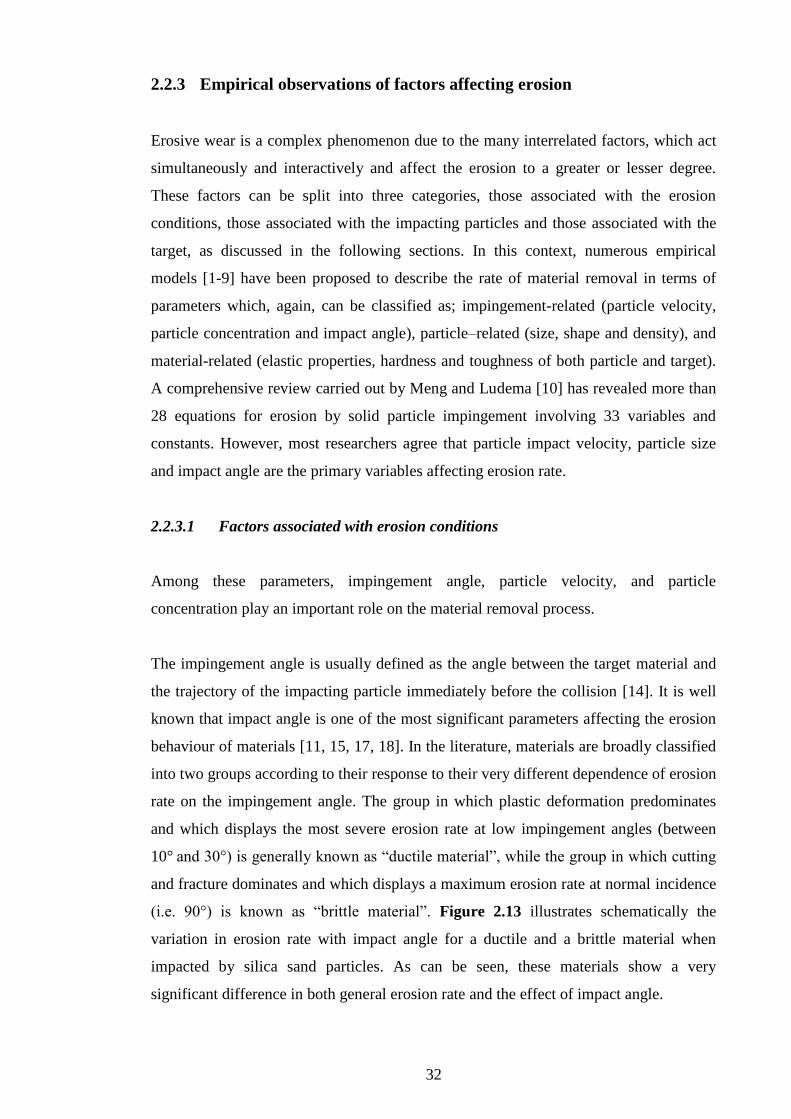
32

2.2.3 Empirical observations of factors affecting erosion

Erosive wear is a complex phenomenon due to the many interrelated factors, which act

simultaneously and interactively and affect the erosion to a greater or lesser degree.

These factors can be split into three categories, those associated with the erosion

conditions, those associated with the impacting particles and those associated with the

target, as discussed in the following sections. In this context, numerous empirical

models [1-9] have been proposed to describe the rate of material removal in terms of

parameters which, again, can be classified as; impingement-related (particle velocity,

particle concentration and impact angle), particle–related (size, shape and density), and

material-related (elastic properties, hardness and toughness of both particle and target).

A comprehensive review carried out by Meng and Ludema [10] has revealed more than

28 equations for erosion by solid particle impingement involving 33 variables and

constants. However, most researchers agree that particle impact velocity, particle size

and impact angle are the primary variables affecting erosion rate.

2.2.3.1 Factors associated with erosion conditions

Among these parameters, impingement angle, particle velocity, and particle

concentration play an important role on the material removal process.

The impingement angle is usually defined as the angle between the target material and

the trajectory of the impacting particle immediately before the collision [14]. It is well

known that impact angle is one of the most significant parameters affecting the erosion

behaviour of materials [11, 15, 17, 18]. In the literature, materials are broadly classified

into two groups according to their response to their very different dependence of erosion

rate on the impingement angle. The group in which plastic deformation predominates

and which displays the most severe erosion rate at low impingement angles (between

10° and 30°) is generally known as “ductile material”, while the group in which cutting

and fracture dominates and which displays a maximum erosion rate at normal incidence

(i.e. 90°) is known as “brittle material”. Figure 2.13 illustrates schematically the

variation in erosion rate with impact angle for a ductile and a brittle material when

impacted by silica sand particles. As can be seen, these materials show a very

significant difference in both general erosion rate and the effect of impact angle.

33

Figure 2.13: Effect of impact angle on erosion for brittle and ductile materials [17]

Al-Bukhaiti et al [49] investigated the effect of impact angle on slurry erosion

behaviour and mechanisms for two materials, 1017 steel (ductile) and high-Cr white

cast iron (brittle), using a constant impingement velocity in a whirling arm slurry test

rig. In addition to its well known effect on erosion rate, impact angle was found to

influence significantly the erosion mechanism involved. Al-Bukhaiti et al concluded

that the main erosion mechanisms for 1017 steel could be divided into three regions,

according to impact angle (see Figure 2.14).

1. Region of small angles, Ө<15o, where shallow ploughing is the predominant

erosion mechanism.

2. Region of intermediate angles, (15o<Ө<70

o), where deep ploughing and

micro cutting are the main erosion mechanisms.

3. Region of high impingement angle, (70o<Ө<90

o), where indentation and

material extrusion are dominant.

34

Figure 2.14: Variation of erosion rate and erosion mechanism of 1017 steel (ductile) as a

function of impingement angle at impact velocity of 15 m/s [49]

The main erosion mechanisms for high-Cr cast iron could be divided into two regions,

(see Figure 2.15),

1. Region of low impingement angles, up to 45o, where ploughing and micro

cutting are the main mechanisms of material removal.

2. Region of high impingement angles, from 45o up to 90

o, involving plastic

indentation with extrusion lips and gross fractures and cracking.

Zhang et al [25] have investigated the effect of impact angle on the erosion of steel

(AISI 1015) under various impact conditions. They reported low wear at very small

angles, reaching a maximum between 20o and 30

o, decreasing steadily until the angle

becomes 80°, finally increasing between 80° and 90°.

35

Figure 2.15: Variation of erosion rate and erosion mechanism of high-Cr white cast iron as a

function of impingement angle at impact velocity of 15 m/s [49]

The velocity of the erosive particles has a very strong effect on the erosion rate [11, 17,

18, 59]. Erosion occurs only when the impact velocity exceeds a critical value known as

the threshold velocity. Yabuki et al [43] found this critical velocity to be dependent on

the mechanical properties of the erosive particles and the target, as well as on the shape

and size of the erodent. For example, they found the threshold velocity to be 2.5 m/s for

0.26 mm silica sand particles impinging on carbon steel. As the velocity increases above

the critical velocity, both the cutting and plastic deformation components increase,

which amplifies the erosion rate drastically. The modes of erosion also vary depending

on the velocity of the particles. At low velocity, the particles do not have enough energy

to erode the material by cutting action, but elastic deformation or fatigue effects may be

observed [42].

Many investigators e.g. [2, 4, 7, 11, 13, 17, 18, 54, 59, 68] agree that erosive wear rates

of materials are strongly dependent on the particle impact velocity and a number have

attempted to correlate the erosion rate with particle velocity. For example, Chen et al

[11] have reported a linear logarithmic relationship between erosion loss and erodent

velocity for both ductile and brittle materials. More generally, the dependence is

commonly expressed as a power law, in which the erosion rate is proportional to the

impact velocity raised to some power n as follows:

36

n

pr kVE

where Er is the erosion rate, k is a constant,

pV is the impact velocity of particles,

and n is the velocity exponent. The value of the velocity exponent n varies with target

material and erodent particle type and many other operating conditions. In a systematic

study carried out by Feng and Ball [13], the erosion of four materials using seven

different erodents has shown the velocity exponent to vary in the range of 1.5-2.7

according to the material properties and erodent characteristics. Ghandi et al [69] used a

slurry pot tester to study the effect of velocity on erosion rate of brass wear pieces at

different concentrations and found an n value of 2.56. Oka et al [53] have examined the

effect of various types of particle on the impact velocity dependence of erosion damage

for both ductile and brittle materials. They found the velocity exponent to vary between

2 and 2.9 for (ductile) aluminium alloy, and between 2.1 and 3.1 for (brittle) cast iron

material. Harsha and Thakre [18] observed velocity exponents are in the range of 2-2.8

for various polymer composites at different impingement angles (15°-90°) and impact

velocities (30-88 ms-1

).

Since the impact velocity has such a significant influence on the erosion rate, it is

important that its value can be controlled and measured. Accordingly, several methods

have been implemented in the literature to measure the particle velocity such as a laser

Doppler velocimeter [16], and photographic techniques using a high-speed light source

[4].

It is generally agreed that the erosion rate increases with increasing particle

concentration within a dilute suspension [25, 59, 69] and then decreases when the

concentration rises beyond a critical value. Particle concentration can be defined as the

mass (or volume) of particles present in a unit mass (or volume) of fluid, as a fraction or

percentage [59, 66, 69].

Desale et al [66] reported that the wear rate of aluminium alloy (AA6063) decreases

with increasing solid concentration (10-30 wt%) at all impingement angles between 15°

and 90°, Figure 2.16, attributing this phenomenon to the decrease in collision efficiency

due to increased particle interaction at higher concentrations. Deng et al [58] have

37

observed a similar effect and again ascribed the reduction in erosion rate to the shielding

effect whereby particles act as a defensive barrier, impeding the progress of further

particles travelling towards the surface.

Figure 2.16: Variation of erosion rate for AA6063 material by a narrow size range of particles

(550 µm) with impact angle at different concentrations [66]

On the other hand, some researchers e.g. [25, 59, 69] have examined the effect of

concentration of particles on erosion rate using dilute suspensions where the shielding

effect is less likely and increasing particle concentration might be expected to cause

more particle impacts onto the surface in a given time and hence greater wear. However,

only a very slight increase in erosion rate is observed as a result of increasing particle

concentration [25] and this increase depends on the dominant mechanism of wear when

the particle impact angle changes. At low concentration, these investigators [59, 66]

have proposed a power law relationship between erosion rate and particle concentration

as follows:

kCEr

where Er is the erosion rate, k is a constant, C is the particle concentration, and β is

the concentration exponent. The value of the concentration exponent β was found in the

literature [25, 59, 69] to vary between 0.2 and the expected value of 1 according to the

target material and erodent particle type.

38

2.2.3.2 Factors associated with erodent particles

The properties of the erodent are also very significant in affecting erosion rate [48], with

particle size, shape and properties all having an effect.

The effect of particle on erosion rate has been studied over a number of years e.g. [11-

13, 15, 25, 69, 74]. Gandhi et al [69] evaluated the effect of particle size on the erosion

rate of brass targets by zinc erodents in a slurry pot tester. The erosion rate was found to

increase linearly with increase in particle diameter for all velocities and concentrations

investigated. Using a Coriolis wear tester, Tian et al [74] have examined the same effect

using three different target materials and silica sand slurry with particle size range (25-

1400 µm). For all materials considered (see Figure 2.17), it was observed that larger

solid particles generate more wear damage at a given impact speed and concentration,

not only for the obvious reason but also due to the fact that the larger mass and hence

higher kinetic energy tend to be more effective in getting the erodent onto the surface of

the material, while smaller particles are more likely to follow the streamlines.

Figure 2.17: Variation of linear wear rate with respect to solid particle size [74]

Many researchers have found a strong dependence of erosion on particle size [12, 13,

25, 69], and have used a power law correlation to describe the relationship between

erosion wear and particle size as follows:

39

pr kdE

where Er is the erosion rate, k is a constant,

pd is the particle size, and φ is the

particle size exponent. Reported values of the size exponent φ vary; Feng et al [13]

found it to be in the range between 2.4 and 4 according to the target material and erosive

particle type (e.g. being 3 for silica sand erodents impacting a stainless steel target),

Clark et al [12] found it to be 2 for SiC erodents in the size range between 100 and 780

μm impacting aluminium targets.

Most experimenters prepare erodents by sieving materials into fractions that will

contain a distribution of sizes between the mesh sizes of the upper and lower sieves, and

so some uncertainty is always associated with the size range distribution of any given

erodent sample [12]. Notwithstanding this, Zhang et al [25] have observed a linear

relationship between the amount of wear and the particle size for gas-solid erosion when

the average particle diameter is <350 μm, but a stronger linear dependence was

observed beyond 350 μm.

Erosion is also affected by the shape of the erodent particles, which are usually

classified as round, angular, or semi-round, based on visual observation. Many naturally

occurring particles are rounded and uniform, but newly or artificially-formed particles

can be sharp and complex, and difficult to describe in simple quantitative terms. The

general shape of a particle is an indicator of its erosive effect; for instance, irregular

shapes with sharp edges increase erosion rate, whereas blunt particles with round edges

retard it [42]. Desale et al [67] have investigated the effect of erodent shape on erosion

wear of two ductile materials by using three different erodents; quartz, alumina and

silicon carbide. They compared erosion rates for two shapes of particles, spherical and

angular, having the same size and density (see Figure 2.18) and pointed out that the

reduction in contacting area of angular particles leads to an increase in kinetic energy

dissipated per unit area, leading to higher stress intensity which enhances the severity of

impact.

40

Figure 2.18: Contact area due to impact of spherical and angular particles [67]

It is well established that more angular particles penetrate more deeply and cause more

effective material removal than do spherical particles, if all other factors remain the

same [4, 14, 74]. The effect of erodent shape was found by Desale et al [67] to be more

dominant at shallow impact angles compared to high impact angles. They suggested that

the erosion rate by angular particles is higher than rounded particles because they were

observed to produce deeper craters and higher average surface roughness.

Chen and Li [11] have simulated the erosion process using a computer model (two-

dimensional, micro-scale, dynamic model) and have investigated the influence of

particle shape, including triangular, square, and circular cross-sections on erosion. The

highest calculated single particle impact erosion loss in the orientation shown in

Figure 2.19 was by triangular particles followed by circular then square particles. This

observation was attributed to the contact area of each particular shape and its

consequent contact stress.

41

Figure 2.19: Erosion rate due to particles of different shapes [11]

The effect of particle shape has also been studied in detail by Winter and Hutchings [46]

who introduced the term ‘‘rake angle’’ to denote the angle between the front face of the

particle and the normal to the target surface. This angle is dependent on the particle

shape, for example always being large and negative for spherical particles. They showed

that rake angle caused a change in erosion mechanism from a ploughing or smearing

type of impact crater with large rake angles to a cutting mechanism at small rake angles.

Angular particles were generally found to cause a greater proportion of cutting type of

material removal [13].

As might be expected, the particle property which most affects erosion is the hardness

relative to the target material. For example, Truscott [15] indicated that, for metals in

general, wear increases rapidly once the particle hardness exceeds that of the metal

being abraded. Beyond this, the wear rate may become fairly constant or may even

reduce with increasing abrasive hardness. The same effect was observed by

Sundararajan and Roy [14] who pointed out that, as long as the hardness of the erodent

is at least twice that of the target material, the erosion rate is independent of particle

hardness. Feng et al [13] studied the effect of eight erodents of different hardness on

erosion rates for brittle and ductile materials. It appeared from their results that the

erosion rate increases with particle hardness once the particles are harder than the target

to be eroded. They also noted that the dependence of erosion rate on particle hardness

and toughness is stronger for brittle materials than for ductile materials.

42

2.2.3.3 Factors associated with target material

A wide range of materials including metals, ceramics, and polymers are used in

applications exposed to erosive environments and the characteristics of these materials

have a strong effect on erosion. Chemical composition, elastic properties, hardness [74]

and surface morphology [67] are some of the major parameters of the target materials

which affect the erosion rate. Among these, hardness is the most widely used target

property to control erosion rate and its effect has been explored by many investigators

[4, 13, 74]. When hard angular particles strike a relatively soft target, the target surface

will deform plastically. On the other hand, when soft erodent particles are used, they

may fracture upon impact, and hence, erosion damage will decrease as the target

hardness increases.

Levin et al [16] have investigated the effect of target material hardness and toughness

on erosion resistance. It was noted that, at low particle velocities, materials with high

hardness may offer good erosion resistance. However, at high particle velocities, when

plastic deformation and/or cracking are more likely, hardness may not improve the

erosion resistance of the target. They concluded that materials that combine high

hardness (which reduces the energy transferred from the incident particle into the target)

and toughness (the ability of the target material to absorb this energy without fracture)

may offer high erosion resistance.

Using a slurry jet impingement rig, Wood [76] has correlated erosion rates, expressed as

volume loss (μm3) per particle impact, with material surface hardness for 21 typical

engineering surfaces including both ductile and brittle materials. He reported that the

erosion rate of brittle materials is more sensitive to hardness with erosion rate

proportional to H -3.2

(see Figure 2.20) while ductile surfaces showed erosion rates

proportional to H -1.6

, where H is the surface hardness.

43

Figure 2.20: Effect of hardness on erosion rate for a range of ductile and brittle materials [76]

2.2.4 Erosion models

Erosion models are useful for the design of slurry components and, in the context of this

work, are also useful in designing experiments which are relevant to real systems.

Over the last 50 years, many models have been proposed to evaluate the rate of material

removal under various eroding conditions. The pioneering work in the prediction of

cutting action damage due to the impact of single particles against a ductile target was

due to Finnie [4]. In his model, the particles were assumed to be rigid (non-deforming)

with sharp edges and the target was assumed to reach a constant flow pressure (perfectly

plastic target) immediately upon impact. Finnie further assumed that no rotation of the

particle occurs during the impact process and hence was able to solve the equation of

motion for the particle trajectory as it cuts the surface by considering all forces acting

on it, and thus predicting the shape of the crater or scratch left by the impacting particle.

The resulting expression was further extended to take into account impacts by several

free moving particles of total mass, M. This resulted in two expressions for total

volume, Q, removed by cutting wear,

for

for

44

where pV is the velocity of the particles, θ is the impingement angle and P is the flow

pressure (constant horizontal pressure between particle and target).

Finnie indicated that no erosion could occur at normal impingement impact, which is

contradictory to other works [6, 61] and noted that the prediction of material removal

for brittle materials is difficult to obtain due to the complex nature of cutting of such

materials [26].

Finnie’s theory formed the foundation for later models, and a more general model was

developed by Bitter [2, 3] who considered both ductile and brittle materials. The Bitter

model makes the hypothesis that the loss of material is the sum of material lost due to

plastic deformation, DW (deformation due to repeated impact of particles normal to the

target where the material elastic limit is exceeded and the surface layer is destroyed and

fragments of it are removed), and that lost due to cutting deformation CW (when the

particles strike the body at an acute angle scratching out some material from the

surface). Using an approach based on Hertzian theory and making use of the energy

balance equation, Bitter derived an equation for deformation wear, WD using a

deformation wear factor, ε, which is the ratio of the energy absorbed by the surface

layer during collision and the amount of energy needed to remove a unit volume of

material:

This equation is valid if yp VV sin , where

yV represents the maximum particle

velocity at which the collision is still purely elastic and hence no deformation wear

occurs. The effect of target mechanical properties on deformation wear is encapsulated

inyV , which can also be considered to be a threshold velocity, below which deformation

wear does not take place and is given by Equation 2.9.

The velocity of impinging particles can be resolved into two components, one normal to

the surface (V1) which is responsible of the particle penetration into the target and one

parallel to the surface (V2) causing a scratching action. Depending on whether the

parallel component of particle velocity becomes zero during the collision process, two

45

expressions of the material removed by cutting wear can be suggested. In the first one

the particle velocity has a parallel component to the surface when it leaves the target

and the material removed is given by:

0,sin(

)sin(cos

)sin(

)sin(22

22

1 VV

VVKV

V

VVMKW

p

yp

p

p

yp

C

On the other hand, if the velocity component parallel to the surface becomes zero during

the collision, the expression for the material removal due to cutting action is

0,

sincos2

1

2

2

3

1

22

2 V

KVKVM

WTp

C

where, K and K1 are constants which depend on material properties, ς is a cutting wear

factor which is defined as the quantity of energy needed to scratch out a unit volume

from a surface.

The total wear in any instance is therefore,

1CDTOT WWW or 2CDTOT WWW

Finnie’s restriction of no particle rotation during the impact process was removed by

Hutchings et al [5-7] who developed a rigid-plastic theory (the particle is undeformable

and the target reaches the fully plastic condition very quickly in the impact process) to

predict collision kinematics and crater dimensions for impacts of single spheres and

square plates on ductile targets. The theory assumed that the elastic effect can be

neglected and predicted the kinematics of the particle as it ploughs or cuts through the

material, under the assumption that the instantaneous resisting force could be calculated

by multiplying a constant plastic flow pressure by the instantaneous contact area.

Because the contact area changes as the particles travel through the target material, the

force resisting the particle motion changes in both direction and magnitude. Hutching’s

theory thus resulted in equations of motion for the particle that had to be solved

numerically, and comparison with experimental measurements of crater volume, energy

loss, and particle kinematics revealed a reasonable agreement.

46

Hutchings’ theory was subsequently generalized by Papini and Spelt [8, 9] so that the

impact of particles of arbitrary shape against targets of arbitrarily dynamic hardness and

dynamic friction coefficient could be analysed. Papini and Spelt [9] further studied the

special case of two dimensional ‘diamond particles’ of various angularities by

constructing a computer programme capable of describing the trajectories of particles as

they form impact craters, so that their size and shape can be predicted. Experimental

work carried out by Papini and Dhar [77] has shown that the agreement between

experimental and predicted rebound linear, angular velocity, and energy loss was good,

while the model generally overestimates the measured crater volume, and

underestimates the rebound angle.

In addition to the contact mechanics-based approaches discussed above, empirical

correlations between impact parameters and erosion damage caused by solid particle

impact offer an alternative approach taken in the literature in order to estimate the

material erosion rate [16, 53]. Based on empirical expressions derived from a wide

range of experiments and observations, the simplest way of writing an equation for

erosion is parametrically [42]:

Erosion = f (operating condition, properties of particles, properties of base material).

However, each equation reflects a very specific and individual case and there are no

predictive equations for erosion damage that can be applied to many types of metallic

materials under various impact conditions. The great variability of the such models

together with the high expense involved in carrying out erosion experiments has led

some authors [78] to develop a numerical model based on the finite element method to

evaluate the removed volume of material due to particle impacts.

2.2.5 Particle interference effects

The work reviewed above focuses on the analysis of single particles striking a surface,

but the importance of multiple overlapping impacts in real eroding flows is now

recognized and currently receives considerable attention. In solid particle erosion

testing, the dependency of the erosion rate on incident particle flux (stream density) can

be attributed to the effects of interference between impacting and rebounding particles

in the collision zone, an effect that limits the erosive potential of the particles at the

47

surface and hence reduces the efficiency of solid particle erosion with increasing

particle flux. Shipway and Hutchings [79] considered the interference between an

incident stream of particles and those rebounding from a flat surface. They describe a

method to determine experimentally both the particle flux below which inter-particle

collisions are insignificant, and the spatial distribution of particles in the incident

stream, for a sand blast type erosion setup. The method is based on the observation that

the erosion scar produced by particles impinging on a coated substrate abruptly

increases in size at a critical particle flux. This increase in scar radius is attributed to

increased particle interactions, as incoming particles are scattered by rebounding

particles.

A computer model that simulates a stream of spherical particles impacting a flat surface

was devised by Ciampini et al [80, 81] in order to determine the interference effect

between rebounding and incident streams of spheres. The simulations allowed for

multiple spherical particle collisions by tracking the movement and collision of

individual particles in three dimensions, so that interference effects could be determined

as a function of stream angle of incidence, incident particle velocity and size, nozzle

divergence angle, particle flux, stand-off distance, and coefficient of restitution for both

particle-particle and particle-surface interactions. A dimensional analysis allowed for

presentation of generalized results, and a parametric analysis identified the

dimensionless groups that were proposed to assess the reduction, due to interference

effects, in stream power from that available at the nozzle exit. In erosion testing, to

avoid confusion between effects due to interference with more fundamental parameters

such as particle size, shape, angle of attack, and material, care must be exercised to

ensure that the particle flux is low enough that only a small proportion of incident

particles undergo collisions. Ciampini et al [80, 81] show that the results of their

simulation can be used to determine the optimum particle flux to be used in such

experiments.

A number of investigators have attempted to construct models that allow assessment of

particle interference effects to be measured analytically [82, 83]. Gomes-Ferreira et al

[84] have simulated particle streams allowing for divergence and for inter-particle

collisions both on the way to the surface and after rebound. Modifying the model of

Shipway and Hutchings [79] for the probability density function (p.d.f.) of particle

angles: , where τ is a dimensionless parameter

48

describing the tendency of the stream to diverge, Gomes-Ferreira et al developed an

expression for the radial distribution of dimensionless incident energy per particle in a

diverging stream with no collisions:

, where the subscript 0% indicates no particle

interference effect, r1* is a dimensionless radial position equal to , where s is the

nozzle-to-surface stand-off distance, and r is the radial distance from the centre of

impacting stream.

When collisions are taken into account, two distributions arise, one for particles which

reach the surface without colliding with other particles:

and one for particles which collide before they reach the surface:

where c is the proportion of particles which collide with others before reaching the

surface, *r and *r is the average dimensionless radius at which

particles which do not collide with others strike the surface. All of the parameters c,

*r , α, A, B, C, D, E, F, G, H and M were determined by fitting the above distributions

to the results of simulations of the particle stream and the entire distribution was

obtained by adding the two.

Simpler distribution functions of particle energies have been considered for other

situations where the flux and velocity are somewhat lower. For example, Crespo [85]

has taken the energy p.d.f. of balls in a ball mill to be given by a Boltzmann

distribution:

1exp

eg e

P P, where P is the average energy.

In a rather different sphere of engineering Brodie and Rosewell [86] have considered

the intensity of rainfall in models of particle wash-off. Whereas these authors were

primarily interested in the total kinetic energy of a given storm, they calculated this

from an empirical distribution of raindrop size, D:

0 expVN D N D

and an empirical relationship between raindrop size and velocity:

49

4.854 exp 0.195FV D D

2.2.6 Particle-laden liquids

The presence of a liquid carrying the particles influences the movement of the abrasive

particles near the test surface much more than in dry erosion. Therefore, it is necessary

to understand the fluid dynamic behaviour of particle-laden liquids and their interaction

with flat surfaces.

Turenne et al [87] have investigated the effect of particle concentration in a slurry on

the erosion rate of aluminium samples using a narrow slurry jet of (200-300 μm) sand

particles in water at normal incidence angle at a fixed velocity of 17 ms-1

, whilst varying

the slurry concentration between 1 and 20% by weight. They characterised the so-called

“blanketing effect” in dense slurries by identifying an erosion efficiency, ηe, (ratio of

mass lost by erosion to mass of erodent used) which decreased with the inverse cube

root of the volume fraction of sand in the stream, f:

0.33e

K

f

where K is a constant which will depend on the erodent, the target, the jet size and the

fluid velocity.

On examination of the eroded surfaces, Turenne et al also noted that they expected that

different impingement angles could result in very different effects of slurry

concentration even to the extent that efficiency could increase with concentration at low

angles of incidence.

Fang et al [88] directed a jet of silica sand (particle size 600-850 μm) suspended in

water at samples of four different ceramics and found that the erosion rate did not

change in a consistent way in the concentration range 3 to 7.5 wt.%, although the

maximum erosion rate for all the materials investigated was at an impact angle of 90°.

Iwai et al [89] investigated the slurry wear rate of 13 materials and found that the effect

of changing one of the experimental conditions such as jet velocity Vj, particle size D,

or particle concentration C on the erosion rate of the target Er was characterised

50

typically by exponents whose values were chosen to fit the experimental data as

follows:

Particularly when the carrier fluid is a liquid, fluid-particle-surface interactions can have

a significant effect on particle trajectories and velocities near the target, and hence on

the AE energy transferred to the target. Laitone [90] was one of the first to comment

that particles approaching a surface always impinge with angles of less than 90o

indicating that there is always a difference between the true incidence angle and the

angle of the approaching flow. Benchaita et al [91] have noted that the form and

dimensions of the erosion crater in a copper target subject to a 20 mm square section jet

consisting of a 0.3 wt.% suspension of silica sand in water were consistent with a spread

in particle trajectories from normal to more inclined angles. They identified three

regions in a jet with normal incidence; a uniform flow at the nozzle exit, a streamlined

flow near the target and a uniform exit flow parallel to the surface. In the streamlined

region, the components of the flow are given by:

and

where x and y are measured from the stagnation point and Z is a flow parameter which

depends on the jet velocity, the nozzle width and the stand-off distance. These authors

also noted that the boundary layer thickness, given by (where ν is the

kinematic viscosity of the fluid), relative to the particle size is important in assessing the

extent to which the boundary layer will slow the impinging particles.

Clark and Burmeister [92] have identified the role of a “squeeze film” as a cushion

between an approaching particle and a surface, irrespective of particle size and initial

velocity of approach. They suggested that the extrusion of the intervening layer may

even prevent impact entirely at low Reynolds numbers, a suggestion which was

confirmed later by Wong and Clark [93] who showed that, for 50 μm glass beads in a

flow at 6 ms-1

, impact is prevented altogether. More recently, Clark [64] has noted that

knowledge of the flow conditions close to the surface in erosion testers, such as the

slurry pot, is “not very sound”, but that the impact velocity of particles, deduced from

individual crater dimensions, can be 50% or less of the free stream velocity of the fluid.

Much of this difference could be explained by potential flow, taking into account the

distribution of impact angles and consequent components of the velocity normal to the

51

target, and the rest was attributed to the retardation effect of the squeeze film, with

small (<100μm) particles in dense slurries being most susceptible. Not only may

particles approaching the target surface at low Reynolds number be unable to penetrate

the squeeze film on rebound or approach and, in more concentrated slurries, a layer of

particles can become trapped at the surface offering the target some protection from the

effect of impact by further approaching particles.

Turenne and Fiset [94] solved numerically the differential equations for particle

movement in the flow field near the surface for a slurry jet impinging a surface with

normal incidence. By curve-fitting their numerical results, they produced parametric

equations for particle trajectories in terms of the final radial position of the particle on

the surface, r, the incident speed V, and the impact angle θ as a function of initial

location of the particle in the jet, ri, the initial velocity (jet exit velocity) Vj, and the

particle size d:

(2.15)

Turenne and Fiset noted that the predominant variable affecting the impact parameters

is the particle size. Due to their higher inertia, the trajectories of larger particles are

deflected less, resulting in an impact angle closer to the original jet direction and the

impact velocity is also a higher proportion of the original jet velocity.

2.3 Acoustic emission (AE) technology

All solid materials exhibit some degree of strain under external forces and will spring

back when released. If this spring back is rapid, such as might occur during incremental

crack propagation or even the sudden movement of dislocations in plastic deformation

the recoil can generate an elastic wave. Such rapid releases of elastic energy caused, for

example, by deformation or damage within or on the surface of a material and the

associated stress waves (essentially propagating elastic strains), are normally referred to

as acoustic emission (AE) [95]. A generating event (source) produces an elastic wave

which propagates in all directions in the body and on the surface and can be detected by

52

locating sensors at appropriate positions on the surface of the object to be monitored, as

shown schematically in Figure 2.21. Sources of AE in rotating fluid-handling

machinery include impacts, fatigue, friction, turbulence, cavitation and leakage [96].

Figure 2.21: Working principle of AE technique [95].

2.3.1 Characteristics of “hit-based” AE

In the current work, the primary interest is in the AE generated by impacting particles,

the monitoring principle being that each particle impact will act as a generating event,

and the cumulative effect of a number of these events can be recorded using AE sensors.

AE is unlike other non destructive methods in many regards [96]:

AE offers the advantage of earlier defect/failure detection due to the increased

sensitivity to the events leading to failure.

Instead of supplying the energy to the object under examination, AE simply

listens to the energy released from the object.

AE is sensitive to the degradative processes, for example, defect growth or

changes in the material, rather than to the static presence of a defect and this is

particularly meaningful because only active defects will be detected. It is

therefore primarily an in-service monitoring tool as opposed to an out-of-service

testing tool.

AE has the ability to monitor simultaneously the entire structure without taking

it out of service. This can offer great cost savings compared to other tests,

53

although more advanced processing is required to interpret the signal if multiple

sources of AE are present or if it is necessary to locate the source.

AE wave types cannot be controlled, and the different wave types travel over

different paths and at different speeds according to the shape and properties of the

propagation medium and surrounding media [97]. At any point on a surface, AE

waves are subject to refraction, scattering, attenuation and reflection from the

boundaries, all of which makes interpretation difficult. Whereas it is rarely the case

in real systems, AE waves are normally treated as if they were pure modes; the most

commonly considered being dilatational (compression) waves, distortional (shear)

waves, surface waves (Rayleigh) and plate waves (Lamb).

AE covers a wide frequency range (100 kHz to 1MHz), and recorded AE signals can

broadly be categorised into burst, continuous and mixed type (see Figure 2.22). In

the first type, the signal can be characterized by discrete transients with relatively

short decay time and even shorter rise times, this type of signal is observed in

unsteady process such as cracking in materials [98]. Continuous emissions are either

bursts that occur too closely together to be distinguished or are due to sources that

are spread out in time. Examples of the former type of signal might be those

associated with plastic deformation in ductile materials and erosion processes in

brittle materials [70]. The final type of AE signal is called mixed mode which

contains a number of high level bursts above the background continuous emission

[99], and are typical of sources which are themselves have some kind of temporal

structure, often those where the source is distributed, such as in engines.

Figure 2.22: AE signal wave types [43]

54

Typical parameters used to describe time-based AE signal features are shown in

Figure 2.23 and these can be summarised [37]:

AE energy is calculated from the integral of squared amplitude of signal

duration over time.

AE count is the number of times that burst signal amplitude exceeds the

preset threshold.

RMS AE is the energy rate or the root mean square of voltage, which is

generally an indicator of average AE energy over each averaging time.

Rise time is the time interval between the first threshold crossing and

maximum amplitude of the burst signal.

Signal duration is the time interval between the first and last threshold

crossing of the burst signal.

However, these descriptors have evolved from the needs of hit-based inspection systems

(aimed at identifying and timing of single events) and they are rarely used as the only

means of analysing the more complex time series typical of a monitoring application.

Figure 2.23: Traditional time-based features of AE signals. Adapted from [99]

55

Signal processing is probably the most important single entity in a condition monitoring

system since it is the means of determining the condition of the system from one or

more complicated time-series signal. Arguably, AE signals contain too much

information, since signals, as acquired, have a bandwidth of 0.1-1MHz. The extraction

of a set of diagnostically significant features from such a signal is the role of signal

processing and this normally requires to be carried out automatically in a real

application. The main aims of signal processing are therefore [100] to:

Reduce the information to a manageable amount.

Reveal the signal features which are of interest.

Minimise the influence of unwanted effects on the signal.

2.3.2 Application of AE as a tool to monitor erosion damage caused by

solid particle impacts

Monitoring of particle impact using acoustic emission exploits the fact that, when a hard

solid particle strikes a target, a fraction of the incident energy dissipates as elastic

waves, which will propagate through the target material according to its shape and

elastic properties before being detected by a suitable AE sensor. The characteristics of

the observed signal from the sensor will depend not only on the particle impact

dynamics, but also upon the propagation of waves into the target medium and the type

of sensor used. Because of this, and the very high temporal resolution available from

AE, and despite the theoretical observation that little of the energy in particle impact is

converted to elastic waves (AE), the potential of AE to monitor erosion phenomena has

attracted many investigators, some concentrating on measuring the erosion variables

identified in section 2.2.3, and others concentrating on monitoring the amount of

erosion. It should, however, be noted that AE monitoring is indirect, in that, at best, it

will reveal the characteristics of the impacts rather than the effect that these impacts

have on removing surface material.

One of the seminal studies of hard particle impact on surfaces using acoustic emission

was by Buttle and Scruby [62] in which bronze and glass particles were allowed to fall

under gravity in a vacuum onto a specimen onto whose opposite face was mounted an

AE sensor of very high fidelity. Using a calibration with a capacitance transducer and

pulsed laser, they were able to deconvolve the AE signal to produce force signals for the

56

impacts, and showed that the peak force and impact times were consistent with

Hutchings’ model [34] for impact time:

, where A is a constant, ρp, R and Vp are the density, radius and

impact velocity of the particle, and f(E) combines the elastic properties of the particles

and target:

2 2

1 2

1 2

1 1f E

E E

The peak impact force indicated by the Hutchings model:

, where B is a constant, somewhat overestimated the

experimental peak forces for some impacts, an observation which was attributed to

possible overestimates of velocity, a non-unity coefficient of restitution and non-

spherical particles. Nevertheless, Buttle and Scruby concluded that, in the range of

impact speeds of 2.5 to 7.1ms-1

and particle sizes 50-100μm, particle size could be

distinguished using AE provided that individual impacts are separated by at least 1ms.

Boschetto and Quadrini [101] have taken a different approach, dropping a fixed weight

of powder of various materials and sizes, and measuring a normalised number of counts,

which they found to be simply related to the mean particle diameter. At the other

extreme of particle flux, Ivantsiv et al [102] have measured the mass flow rates of

particles in abrasive jets using AE. Glass beads of approximately 60 μm nominal

diameter and aluminium oxide powder of 25 μm equivalent spherical diameter were

used as abrasives with particle velocities of around 150ms-1

and particle impacts

separated by around 30-100μs. They used two approaches to estimate the mass flow rate

(controlled to be between 1 and 11 g min-1

), the first using a dynamic threshold to count

individual impacts and the second using the power spectral density (PSD) of the AE

signal. Also working with high particle fluxes (80 g min-1

of 18-80 μm equivalent

spherical diameter particles), Faisal et al [103] showed that the measured AE energy

and expected kinetic energy rate in HVOF spraying were well correlated. In both of

these pieces of work, it was necessary to mask the surface to limit the number of

incident particles. The simple kinematic model for spraying through a slit used by Faisal

et al [103] assumed that the particle velocity and density was constant across the

impinging spot and the particle spay was collimated.

57

Duclos et al [22] carried out a rather more applied study using AE to monitor impacts of

streams of particles of various sizes at various concentrations in a water flow loop. By

estimating the number of impacts from the particle concentration and flow rate, they

showed that the AE energy per particle was approximately proportional to the cube of

particle size (i.e. particle mass), although they noted anomalies at higher particle sizes,

attributable to particle drop-out according to Stokes’ Law. Some authors have reported

the possibility of using an AE sensing technique for on-line monitoring of slurry flow

properties. Hou et al [23] mounted an AE sensor on the external wall of a small

diameter pipeline conveying dense slurries of fine silica particles with an average

particle size of 13 μm. Based on the acoustic noise produced by the fluid flowing inside

the pipeline and using a stepwise regression analysis technique, they were able to derive

quantitative relationships between the physical properties of the flow, such as solid

concentration, mass flow rate and volume flow rate, and the statistical and spectral

characteristics of the recorded AE. They also observed that the frequency in the power

density spectrum of the signal increased with increasing flow rate. However, the

validity of this empirical regression approach depends upon the mechanical flow

properties of the two-component mixture, and is unlikely to be applicable on all other

configurations where different components and materials might be involved.

Ferrer et al [20, 21] attempted to characterize and understand the mechanical damage

during the abrasion-corrosion process with the aid of a combination of AE measurement

and an electrochemical device used for corrosion potential measurements. A slurry jet

impingement rig was used with the potential of varying fluid flow rate (1-16 ms-1

),

concentration (1-8 wt.%), and angle of impact (30°-90°) with an AE sensor coupled on

the rear surface of the 304L stainless steel target. Two different methods were studied.

For the single impact method, where glass beads of diameter 720 μm were introduced

into the suspension one by one, they observed that the acoustic energy due to the impact

is proportional to the incident kinetic energy. The coefficient of proportionality was

found to increase with the impact angle, and this observation was attributed to the

hydrodynamic boundary layer that slows the particles at low impact angle as well as

lowering the amount of elastic energy transmitted to the target. They also observed that

the amplitude and the frequency of the AE bursts increase with the velocity of the fluid

(which was assumed to be the same as the velocity of the particles). When the particle

velocity was greater than 10 ms-1

, new bursts characterized by low amplitude and low

frequency parameters were observed. These new bursts were attributed to bubbles

58

generated in different locations on the test loop and it was concluded that AE was

capable of separating easily the impact of particles from the collapse of bubbles, an

observation confirmed later by Duclos et al [22], who reported that acoustic energy due

to air bubbles is much lower than that for particle impacts. Both sets of author concur

that bubble collapse is unlikely to constitute a significant uncontrolled source of

acoustic emission in systems where abrasion and erosion need to be monitored. For the

multi-impact method, where defined quantities of SiC particles of size 125 μm were

introduced into the suspension, Ferrer et al [20] obtained a simple relationship between

the weight loss measured at the end of the test (2 hours) and cumulated acoustic energy

measured during each test. On this basis, they claimed that acoustic energy may used to

quantify the mechanical damage due to abrasion-corrosion processes, whatever the flow

rate and the concentration of particles, although clearly some kind of calibration would

be required.

Oltra et al [73] used AE to monitor combined abrasion and corrosion of stainless steel

plates with a slurry jet impinging normal to one surface and an AE sensor fixed on the

other. They measured the relative amounts of erosion and corrosion, and showed that

the mechanical wear (measured as a mass loss after the 1 hour erosion test) was

proportional to the mean value of RMS AE signal for the duration of the test. However,

in parallel experiments with individual impacts using spherical glass beads of various

diameters (from 1 to 2.5 mm) and SiC particles of various sizes (from 1 to 2.8 mm),

they observed that the acoustic emission was proportional to the kinetic energy of the

particle impact and not to the mechanical damage, measured as the volume of the wear

crater which was determined after averaging the mass loss due to several impacts.

Burstein and Sasaki [24], as well as concurring with the observation [73] that the wear

rate by particle abrasion is correlated to the RMS AE signal, further indicated that using

either the maximum amplitude of individual AE events or the RMS AE value was an

acceptable measure of the magnitude (wear induced) of the impact in slurry handling

after a clear linear correlation between RMS AE signal and maximum amplitude of

individual AE events was found. Using a slurry jet impingement rig to study the effect

of impact angle on slurry erosion-corrosion of a stainless steel target, they examined the

correlation between the maximum amplitude of AE events and the electrochemical

transient caused by the impact of an individual erosive particle (400-650 μm rounded

silica sand particles). A high degree of scatter was observed in correlations between

59

current rise and AE amplitude although it was observed that each sharp rise in the

electrochemical current transient under particle impact was accompanied by an AE

event. The correlation was found to depend on impact angle and less scatter was found

at oblique angles than at normal incidence. The sharp current rises were ascribed to the

rupture or removal of oxide film on the surface by the impact of abrasive particles. To

simulate erosion of boiler tubes, Zhang et al [25] directed an air stream with particles

<500 μm onto the surface of a tube while measuring the AE energy. Using dimensional

analysis, they established a relationship between AE energy and the erosion wear,

including erosion parameters: Eg

f

H

p, where ζ is the erosion wear after a given

time, E is the acoustic emission energy, ρp is the particle density, H is the hardness of

the tube material, and f and g are dimensional functions of ,,,pp

p

p H

V

H

dC

where c is the particle concentration, dp is average particle diameter, V is particle

velocity and θ is the particle impingement angle. Zhang et al observed that the

measured AE indicated that low collision angles dissipate less energy than higher

collision angles, an observation which is consistent with [20].

AE has also been proposed as a promising tool for on line monitoring of material

removal involved in the abrasive water jet (AWJ) drilling process. Mohan et al [104]

have investigated the ability of the AE technique to detect the amount of energy

dissipated in the workpiece during such a process. A simple physical model to

determine the absorbed jet energy was developed and correlated to the measured energy

of the AE signals at different water pressures. A logarithmic relationship was found

between the calculated absorbed energy and the measured AE energy which implies the

possibility of using AE as an indicator of energy dissipated during AWJ machining. In

related work, Kovacevic et al [70] used AE to study the material removal mechanisms

involved in the AWJ drilling process for three different materials, magnesia chromite,

sintered magnesia, and bauxite. The time domain AE signals corresponding to the first

material, which is characterized by a lower Young’s modulus and lower cold

compressive strength as well as the presence of hard inclusions in a much softer matrix,

were of continuous type representing a material removal mechanism due to

intergranular erosion or microcracking. The material removal in a highly brittle material

(the second material) was primarily due to continuous propagation of a microcracking

network as was indicated by dense continuous AE. The time domain AE signals for the

60

last material were of burst type which indicated that the material removal mechanism is

of the transgranular fracture type. Moreover, they correlated RMS AE signals with

drilling depth to investigate the feasibility of using AE to monitor the AWJ drilling

depth. Plots of RMS AE against drilling depth for the three materials showed that RMS

AE reduces with increase in drilling depth. This reduction was attributed to the effect of

back flow of the jet which reduces the particle velocity in addition to the damping effect

on the AE signal caused by AWJ debris present in the small diameter hole.

In another area of abrasion study, Momber et al [72] employed the AE technique for on

line monitoring of hydro-abrasive erosion (HAE) of pre-cracked multiphase materials

exemplified by five types of concrete. They investigated the effect of a range of erosion

parameters such as abrasive particle velocity, local exposure time, and abrasive mass

flow rate on the AE signals. They observed a higher amplitude of AE signal at higher

impact velocities and attributed this to the presence of a more powerful material

removal process, whereas, in contrast, the influence of the abrasive mass flow rate was

not very significant. In addition, they found that material removal which is dominated

by intergranular fracture is characterized by continuous AE signals, while material

removal dominated by transgranular fracture is characterized by burst emission due to

the sudden energy release during inclusion fracture. This observation is consistent with

other work [70], and confirms the suggestion that AE is capable of revealing different

material removal mechanisms occurring in materials when subject to HAE.

AE has also been used to monitor sliding wear in various types of laboratory test.

Boness and McBride [105], using a ball-on-cylinder test apparatus, where a stationary

ball is loaded against a rotating cylinder, acquired AE signals from a sensor coupled

acoustically to the ball housing. They obtained an empirical relationship between RMS

AE and the volume of wear removed from the test ball. They also studied the effect of

using different lubricants in the sliding contact on both wear and acoustic emission.

They indicated that RMS AE is quite sensitive to the type of lubricant used (for example,

RMS AE signals were larger for light paraffin, followed by heavy paraffin then smallest

for SAE 30 oil) and were able to characterise the abrasive wear involved in lubricated

sliding contacts. A similar empirical relationship between material removal and RMS AE

was verified later by Matsuoka et al [106]. Another study concerning sliding wear was

carried out by Mechefsek and Sun [107], who used a similar experimental rig to Boness

and McBride in an attempt to distinguish between effective and poor boundary

61

lubrication. In the time domain, they observed that the AE counts were small when the

wear rate was mild (effective lubrication) and large when the wear rate was severe (poor

lubrication). They suggested using either AE peak level or RMS AE values to represent

the wear surface strain rate. This is in agreement with the work of Burstein and Sasaki

[24].

2.4 Identification of thesis topic

It is clear from the foregoing review that AE has been used successfully as a means of

monitoring erosion caused by hard particle impact on a target material. However,

different investigators have made measurements under varying geometrical and

dynamic conditions which in turn lead to results which are often simply correlations and

are not precisely comparable with each other and, indeed, are divergent in some cases.

No model is available so far to link either the material removal or the incident kinetic

energy with AE signals for practical applications. Also, most of the work that has been

done (with a few exceptions) on identifying AE energy with impact energy carries with

it an inherent calibration problem in a system where energy might be lost by

propagation and multiple sources with different propagation paths might be present. The

approach to be taken here, therefore, is to use a standard measurement “cell” consisting

of a target and sensor and to carry out a set of staged experiments where control of the

impact conditions is gradually ceded in the interest of practical applicability, thus

bridging the gap between controlled impact experiments with one or few impacts to

experiments in realistic flow conditions with multiple overlapping impacts and noise

from the carrier fluid.

62

Chapter 3

Experimental method

This chapter describes the solid particle types and specimen details, AE measurement

system, and all the experimental procedures and arrangements for this study including

calibration tests.

First, the materials, AE monitoring apparatus and signal processing techniques are

described. Next, the calibration of the AE sensor using simulated sources on a steel

block and on the target specimen along with the calibration of the specimen for its AE

propagation characteristics are presented. Finally, the details of systematic experimental

procedures for the three types of AE monitoring experiments are presented; free-fall and

air-assisted particle impacts, slurry impact using a slurry jet impingement rig, and

particle impacts in a flow loop bend.

3.1 Materials, instrumentation and signal processing

The experiments essentially consisted of monitoring particles impinging on a steel

surface and, as such, used a common set of materials and equipment.

3.1.1 Particle types and target plate details

The free-fall and air-assisted particle impact experiments used the widest range of

particle types; steel balls, solid spherical glass beads, and angular silica sand. The sizes

and fractions used are listed in Table 3.1. Most of the experiments were performed with

sieved samples of glass beads and silica sand, the sieving having been carried out to

British Standard 410, and size distributions for air-assisted multiple particle impact

experiments are given in Table 3.2. The distribution functions were measured using a

Malvern particle size analyser, an example distribution being shown in Figure 3.1.

These distributions were assumed to be Gaussian and the mean and standard deviation

were obtained by curve fitting to the Malvern data.

For the slurry jet impingement and flow loop experiments, silica sand sieved fractions

were separated with dry sieves from commercial bulk silica sand (from Hepworth

63

Minerals and Chemicals Ltd, UK). The fractions used are listed in Table 3.3.

The geometry of the silica sand was examined using an optical microscope (Nikon, with

N50 monochrome camera) and found to be angular with semi sharp-semi round corners,

as shown in Figure 3.2.

Free-fall experiments

Single particle impacts Multiple particle impacts

Particle

type

Particle size fraction

μm

Particle

type


μm

silica sand

125-212

silica sand

125-180

212-300 180-212

300-425 212-250

425-500 250-300

500-600 300-425

Single particle impacts

Particle

type Particle diameter mm

Particle

type Particle diameter mm

steel balls

1

glass beads

0.9

1.5 1.97

2 2

2.5 3.5

3.2 4

4 6

Air-assisted

experiments

Single particle impacts Multiple particle impacts

Particle

type


μm

Particle

type


μm

silica sand

125-180

silica sand

212-250 125-180

300-425 212-250

500-600 300-425

glass beads

125-180

glass beads

212-250

300-425 500-600

500-600 600-710

600-710 710-850

710-850

850-1000

Table 3.1: Particle types and sizes used in free-fall and air-assisted experiments for single and

multiple particle impacts.

64

Particle type Particle size fraction

(μm) Size distribution function

silica sand

125-180 13448

)175(exp

205

1 2d

212-250 7442

)252(exp

5.152

1 2d

300-425 20808

)320(exp

255

1 2d

glass beads

500-600 5832

)586(exp

135

1 2d

600-710 13778

)668(exp

2075

1 2d

710-850 39762

)776(exp

5.352

1 2d

Table 3.2: Size distribution functions for air-assisted particle impact experiments.

65

Figure 3.1: Measured particle size distribution for glass beads in size range 710-850μm.

Figure 3.2: Silica sand erodent particles of size fraction 300-425 µm.

Particle type Particle size fraction μm

slurry impact experiments

silica sand

125-180

212-250

300-425

Flow loop experiments

212-250

300-425

500-600

600-710

Table 3.3: Particle types and fraction sizes used in slurry impact and flow loop experiments.

Particle Diameter (µm.)

Number (%)

0

10

20

30

0

10

20

30

40

50

60

70

80

90

100

10.0 100.0 1000.0

66

The target material was carbon steel, on which all measurements reported in this study

have been made. For most of the tests, a specially-designed target was made, consisting

of a circular plate of diameter 75 mm and thickness 7 mm, mounted into a sample

holder as shown in Figure 3.3. A purpose-designed clamp with screws was designed to

hold the sensor onto the centre of the rear specimen surface. Great care was taken to

isolate the target material from the surrounding sample holder material both to avoid

noise and to provide reproducible conditions over a range of experiments. For the flow

loop experiments, a sharp 90 degree bend made from 5 mm bore carbon steel was

machined and used as a target (see Section 3.3.3).

3.1.2 AE apparatus

The AE acquisition system is shown schematically in Figure 3.4. The system

comprised a target, an AE sensor, a pre-amplifier, a signal conditioning unit, a

connector block, a data acquisition card and a computer with LabVIEW software for

controlling the acquisition and storage of data in the PC as shown in Figure 3.5.

Impinging

particle

AE sensor

Target Pre-amplifier:

PAC-1220A Elastic waves

Computer

75 mm

7 mm

AE sensor

Sample

holder Target Rubber O-ring

Nylon

insulator

Retaining collar

Figure 3.3: Sectional view of target plate in sample holder

Figure 3.4: Schematic view of the AE acquisition system

67

Figure 3.5: The AE acquisition system

The AE sensor, which was used for all experiments, was a commercially available

“broadband” sensor of type Physical Acoustics (PAC Micro 80 D-93), based on lead

zirconate titanate (PZT). The sensor was 10 mm in diameter and 12 mm in length, and

is not truly broadband but produces a relatively flat frequency response across the range

(0.1 to 1 MHz) and operates in a temperature range of -65 to 177 oC. The sensor was

chosen because of its wide use in other research on machinery monitoring and its

relative robustness. In order to obtain a good transmission between the test object and

the AE sensor, silicone high vacuum grease was applied to the sensor face before

mounting onto the specimen to fill any air gaps caused by surface roughness which

might otherwise impair wave transmission. Before every test, the sensor was checked

by performing a pencil lead break test to ensure proper connection and attachment of the

sensor.

A preamplifier shown in Figure 3.6a, was used to amplify the AE signal to a level that

can be transmitted and read by an ADC of type PAC model 2/4/6, having a switchable

gain (20/40/60 dB) and internal band pass filter from 0.1 to 1.2 MHz to ensure that

electronic noise outside the frequency range of interest is kept to a minimum. The

preamplifier was powered by a +28 V power supply and used a single BNC connection

for both power and signal. A programmable 4-channel signal conditioning unit (SCU)

and a gain programmer (shown in Figure 3.6b) of in-house manufacture were used to

PC with DAQ

card installed

Signal

Conditioning

Unit

68

power the AE sensors and pre-amplifiers as well as to adjust the gain level, if necessary,

to ensure that all relevant parts of the signal could be examined.

Figure 3.6: (a) Pre-amplifier, (b) Signal conditioning unit, connector block and gain

programmer

Different levels of amplification were used both in the preamplifier and the gain

programmer, according to experimental conditions. Prior to any signal processing, all

amplifications due to different gains were normalized using a code in MATLAB.

A National Instruments BNC-2120 connector block (Figure 3.6b) was used to carry

signals from the sensor to the data acquisition system. This was a shielded connector

block with signal-labelled BNC connectors and included a LED to check the

functioning of the hardware.

Since the acquisition of raw AE signals in the bandwidth 0.1 to 1MHz requires a high

sampling rate, a 12-bit resolution National Instruments (NI), PCI-6115 data acquisition

card (DAQ) was used, and assembled into an in-house built desktop PC as shown in

Figure 3.5. The board allowed raw AE to be sampled and stored simultaneously at up to

10 M Samples/s for up to four channels (i.e. 2.5 M samples/s/channel) with a total

onboard memory of 32 MB. The board supports only a differential input configuration

and has a maximum voltage protection of 42 V. LabVIEW software from National

Instruments was used to obtain the raw signals from the PCI-6115 board along with

LabVIEW code [108] to control sampling frequency, number of acquired samples per

channel, number of records, input range, pre-trigger data, trigger channel and trigger

(a)

(b)

69

level. Most of the data in this study were acquired at 2.5 M Samples/s for different

record lengths.

3.1.3 AE signal processing techniques

Once generated, AE waves radiate in all directions, propagating throughout the material

in a variety of forms namely; compression, shear, Lamb and Rayleigh waves. Since the

wave from a point source has a fixed amount of energy, the wave amplitude will

decrease with distance. According to Pollock [109], this phenomenon, known as

attenuation can be attributed to four reasons; geometric spreading of the wavefront,

internal friction, dissipation of energy into adjacent media and velocity dispersion.

Further signal distortion can occur when material boundaries are encountered where

wave reflection, refraction, transmission and mode conversions can all occur. In reality,

this means that AE waveforms are complex and using them to characterise the source

can be difficult as AE signal waveform (amplitude-time) is affected by characteristics of

the source, the path taken from the source to the sensor, the sensor characteristics and

the AE measuring system. Therefore, signal processing is probably the most important

single entity in a condition monitoring system whose aim is to determine the condition

of a system under test. The aim can be translated as the need to extract a set of

diagnostically significant features from the AE waveform.

For this particular application, there are multiple random sources arriving at an area

quite close to the sensor, so some of the more sophisticated methods associated with

source location and propagation are not needed. However, the target plate is thin and

considerable ringing in the target can be expected.

3.1.3.1 Time domain analysis

Time domain analysis involves extracting time features from raw AE time series

signals, which themselves can be categorised as continuous type or burst type. For AE

burst signals, where the amplitude usually rises rapidly to a maximum value and decays

nearly exponentially to the background noise level, a number of conventional features

have been developed to describe the AE burst signal, and these were summarised in

Section 2.3.1.

70

For the purpose of making an assessment of the correlation between particle incident

energy and AE energy for single particle impact experiments, the AE impact energy E

was calculated from the raw signal by integrating over the entire time record t above a

threshold level of 10% of the maximum peak height, (measured as an amplified

voltage, V):

t

dttVE0

2 )(

(3.1)

In practice, even at 2.5 MHz sampling rate, the AE associated with multiple particle

impact events may well overlap. In order to simplify the signal processing for peak

searching, each record was divided into intervals and then the root mean square RMS for

each interval was calculated. It should be noted here that other time domain analysis

using different thresholding techniques are described later.

3.1.3.2 Frequency domain analysis

Frequency domain analysis offers further options for investigation of AE signals. It

involves obtaining signal spectral characteristics to estimate the distribution of the

signal energy in the frequency domain. In general, frequency analysis involves the

decomposition of time-series data into the frequency domain using a Fast Fourier

Transform (FFT) algorithm [110] or Welch’s Power Spectral Density PSD estimate

[111]. Frequency analysis is sometimes used to filter out noise from a signal in cases

where AE sources are masked by the noise or the frequency structure may be used as a

diagnostic indicator itself. In the first of these, if the required filter is carefully identified

and constructed, then this can allow removal of noise in narrow frequency bands and

accordingly enhance signal-to-noise ratios, provided, of course, that the noise has a

different frequency structure to the signal.

Another application of the FFT which is of particular use is called demodulated

resonance analysis [112]. The technique involves averaging the signal using a sliding

root mean square RMS to reveal lower frequencies in the envelope of the signal, where

the AE wave acts as a carrier frequency for the lower frequency information,

Figure 3.7. Again, the structure of the demodulated spectrum can itself be used as a

diagnostic indicator, or can be used to identify, and remove, noise.

71

0 0.1 0.2 0.3 0.4 0.5 0.6 0.7 0.8 0.9 10

0.1

0.2

0.3

0.4

Am

plitu

de (

V)

Time (s)

RMS of raw signal

0 100 200 300 400 500 600 700 800 900 10000

1

2

3

4x 10

-5 FFT of RMS

Frequency (Hz)

Am

plitu

de (

V)

Figure 3.7: Steps of demodulation frequency analysis, (a) raw AE signal, (b) RMS of the AE

signal, using averaging time of 0.2 ms

3.2 Calibration tests

The calibration tests were carried out to determine AE propagation characteristics in

the target and to assess the repeatability and functionality of the AE system. First, the

simulated AE source is described, and then, the three calibration tests for the sensor in

different installations are presented.

All AE signals associated with the calibration tests were acquired at 2.5 MHz for a

record length of 20 ms, and a total of ten lead breaks were performed at each location.

The total energy in each record was obtained using the method described in

Section 3.1.3.1.

3.2.1 Simulated source for calibration tests

A pencil lead break test is a well established procedure for generating simulated AE

sources. Therefore, a commercial mechanical pencil with an in-house machined guide

ring was used to generate simulated AE sources by breaking a 0.5 mm diameter and 2-3

mm length 2H pencil lead, as recommended by ASTM standards (E976-99) [113]. The

so-called Hsu-Nielson source along with its guide ring is shown in Figure 3.8. The

guide ring made it possible to maintain the same orientation of the pencil for all tests

and hence break the lead in a consistent way.

0 0.1 0.2 0.3 0.4 0.5 0.6 0.7 0.8 0.9 1

-1

0

1

Time (ms)

Am

plitu

re (

V)

Raw signal

1 2 3 4 5 6

x 105

0

2

4

6

x 10-7 FFT of raw signal

Frequency (Hz)

Am

plitu

de (

V)

(b) (a)

72

Figure 3.8: Hsu-Nielsen source and guide ring [113]

3.2.2 Calibration tests on steel cylinder

Using a large steel block with a pencil lead break source can provide a reference

calibration for characterizing a sensor. So, AE signals were acquired at four positions

separated circumferentially by 90o on a large cylindrical steel block of dimension 300

mm diameter and 200 mm height as shown in Figure 3.9. The AE sensor was placed on

the surface of the block at the same radial distance (120 mm) from the source at the

centre of the top surface, and was installed and de-mounted 5 times at each position

with records of 10 pencil-lead breaks being acquired each time, so that 50 breaks were

recorded for each position (indicated P in the Figure). Then, the sensor was moved to

another position and the entire process was repeated.

P4

P3

P2

P1 Wooden supports

AE sensor Pencil lead

break

Steel

cylinder

(a) (b)

Figure 3.9: Sensor calibration set-up (a) schematic view of steel cylinder arrangement, (b)

plan view of sensor positions relative to the cylinder and supports

73

Figure 3.10 shows the AE energy recorded for all of the 50 pencil-lead breaks at each

of the four positions, each point showing the average and the variation over the 50 lead

breaks. As can be seen, P1 and P3 show similar (lower) values with less scatter in

recorded AE energy than P2 and P4. This effect is probably due to the configuration

with the wooden support underneath P1 and P3 providing a leakage path.

Figure 3.10: AE energy recorded at the four calibration positions on the steel cylinder

Figure 3.11 shows the energy distribution as average, minimum, and maximum AE

energy recorded, for the five independent trials in which the sensor was removed and

replaced at each of the four positions. As can be seen, the energy recorded for a given

installation varies considerably and this can be attributed to the variation of the pencil-

lead break (within group variation). In addition, the energy recorded between

installations at the same position is different and this is attributed to changes in coupling

conditions and magnetic clamp tightening force. In order to analyse the variance

between a given installation (the effect of de-mounting the sensor) and among

installations (the effect of lead breaks) quantitatively, the data for each placement at

each position was grouped and ANOVA testing was carried out. The indicator Fvalue

was compared with Fcrit (2.57 for the degrees of freedom involved and at the 95%

confidence level) and, as can be seen in Table 3.4, Fvalue is always greater than Fcrit

indicating that the variation due to removal and replacement of the sensor is more

important than the variation in pencil lead breaks at all positions. In addition, the data

for each position was grouped to analyse the variance between positions and among

0.0E+00

1.0E-07

2.0E-07

3.0E-07

4.0E-07

5.0E-07

6.0E-07

7.0E-07

AE

en

erg

y, V

2 .se

c

P4 P2 P3 P1

74

positions which enables the comparison between the effect of position and the effect of

lead break and sensor replacement. This time Fvalue was 74, much greater than Fcrit

indicating that the effect of changing position is more important than the effect of pencil

lead break and sensor replacement.

Figure 3.11: Recorded AE energy for simulated sources at four positions (results of five

independent tests between which the sensor was removed and replaced)

Position Fvalue Fcritc

1 4.56 2.57

2 3.38 2.57

3 5.93 2.57

4 3.04 2.57

Table 3.4: Summary of ANOVA results comparing the effect of demounting the sensor with the

effect of pencil lead breaks at each position

3.2.3 Calibration tests on target

Since the target was relatively small, it was necessary to obtain an indication of the type

of propagation behaviour shown by the wave generated from a simulated source, as well

as understanding any time or frequency domain characteristics introduced by the target.

The AE sensor was placed at the rear surface of the target on its epicentre, as it is placed

for all of the experiments carried out during this study, and AE was recorded with the

simulated source placed at four different positions on the face of the target as shown in

-1.55E-20

2.00E-07

4.00E-07

6.00E-07

8.00E-07

1.00E-06

1.20E-06

1.40E-06

P1 P1 P1 P1 P1 P2 P2 P2 P2 P2 P3 P3 P3 P3 P3 P4 P4 P4 P4 P4

AE

en

erg

y, V

2 .se

c

75

Figure 3.12. Two independent tests were carried out, acquiring ten pencil leads at each

of the four positions, after which the sensor was removed and replaced on the target

plate, giving a total of 20 AE records at each position.

Figure 3.13 summarises the recorded AE energy for the pencil lead breaks at all

positions represented by average points and the range for the ten lead breaks at each

position for each test. It is clear that significant change in recorded AE energy occurs as

the source was moved away from the plate centre. It might be noted that the variation in

AE energy at each position due to the variation of the pencil-lead break was smaller

than the variation due to sensor removal and repositioning as was found in the

calibration tests.

Figure 3.13: Recorded AE energy for simulated sources across the target diameter (results of

two independent experiments between which the sensor was removed and replaced)

Because the experiments involve re-installing the sensor at different times, it was

necessary to establish the repeatability of AE energy measurement and quantify the

effect of sensor remounting at different installations. Therefore, at a fixed position

0.0E+0

5.0E-6

1.0E-5

1.5E-5

2.0E-5

2.5E-5

3.0E-5

3.5E-5

4.0E-5

4.5E-5

5.0E-5

0 5 10 15 20 25

AE

en

erg

y,

V2sec

Distance from the plate centre, mm

Target plate

AE

sensor

2.5 mm 10 mm 10 mm

Pencil break positions

Figure 3.12: Schematic view of the target calibration arrangement

76

(centre of the target plate), 5 pencil lead breaks were recorded in each of ten

independent batches after each of which the sensor was removed and replaced in the

same position. As can be seen in Figure 3.14, the energy recorded between installations

is different and this is might be attributed to changes in coupling conditions and clamp

tightening force.

As with the steel cylinder calibration tests, the data for each installation was grouped to

carry out an ANOVA test. The Fvalue of 4.1 was greater than Fcrit (2.1 for the degrees of

freedom involved and at the 95% confidence level), indicating that the variance

associated with de-mounting the sensor is more significant than that of the pencil lead

break, confirming the finding with the steel cylinder. Therefore, the sensitivity variation

for a given installation (approximately 15%) needs to be taken into account when

comparing measurements made at different times where the sensor has been removed

and re-mounted again.

Figure 3.14: Testing of repeatability of recorded AE energy using H-N source

Figure 3.15a shows the time-domain of a typical raw AE signal due to a pencil lead

break at the centre of the target plate, whereas, using the same sensor, a typical raw AE

signal due to a pencil lead break on the face of the steel cylinder is shown in

Figure 3.16a. To compare these signals Figure 3.16b shows part of the record from

0.0E+00

1.0E-05

2.0E-05

3.0E-05

4.0E-05

5.0E-05

6.0E-05

0 2 4 6 8 10 12

AE

en

erg

y,

V2sec

Installations

Pencil lead break 1

Pencil lead break 2

Pencil lead break 3

Pencil lead break 4

Pencil lead break 5

Average

77

Figure 3.16a expanded to a length similar to that shown in Figure 3.15a. Cleraly both

test objects exhibit considerable ringing with the target plate decaying more rapidly than

the cylindrical block. In order to understand the causes of the ringing, Figure 3.15b and

Figure 3.16c show magnified segments of the records depicted in Figure 3.15a and

Figure 3.16b, respectively. As can be seen, the AE signal in the target plate is of higher

intensity than that in the steel block. Figure 3.16c also shows two clear wave reflections

whose return times are consistent with a Rayleigh surface wave reflecting from the

edges of the cylinder nearest to and diametrically opposite to the sensor, while reflection

from the bottom of the cylinder is not clearly observable above the background. In the

target plate, the return time of a compression wave reflected at both surfaces is

observable, but this time is so short as to be within the period of the AE waves

themselves. These signals indicate a strong influence of the carrier structure on the AE

recorded. Therefore, in order to quantify the effect of the target thickness on AE energy,

Figure 3.17 shows the variation in AE energy for pencil lead breaks on the face of the

target plate and on the face of the steel cylinder, where each point represents the

average, maximum, and minimum of 10 AE records. The high energy recorded for the

target plate is therefore associated with many reflections from the faces and little

absorption at each reflection.

Figure 3.15: Typical raw AE signal for a pencil lead break on the face of the target plate: (a) a

full record, (b) a magnified view of (a)

0 0.5 1 1.5 2 2.5 3 3.5 4-1

-0.8

-0.6

-0.4

-0.2

0

0.2

0.4

0.6

0.8

1

Time (ms)

Am

plit

ure

(V

)

0.38 0.4 0.42 0.44 0.46 0.48 0.5 0.52 0.54 0.56

-0.4

-0.3

-0.2

-0.1

0

0.1

0.2

0.3

Time (ms)

Am

plit

ure

(V

)

(a) (b)

78

Figure 3.16: Typical raw AE signal for a pencil lead break on the face of the steel cylinder: (a)

a full record, (b) a magnified view of (a), (c) a magnified view of (b)

0 10 20 30 40 50 60 70 80-0.08

-0.06

-0.04

-0.02

0

0.02

0.04

0.06

0.08

0.1

Time (ms)

Ampl

iture

(V)

0 0.5 1 1.5 2 2.5 3 3.5 4-0.08

-0.06

-0.04

-0.02

0

0.02

0.04

0.06

0.08

0.1

Time (ms)

Ampl

iture

(V)

0.38 0.4 0.42 0.44 0.46 0.48 0.5 0.52 0.54 0.56

-0.08

-0.06

-0.04

-0.02

0

0.02

0.04

0.06

0.08

Time (ms)

Ampl

iture

(V)

(b)

(c)

(a)

79

The decay time was obtained from the AE records as the time between the first and final

appearance of the AE above a threshold level of 15% above the continuous background

level. Figure 3.18 shows the variation in AE decay time for pencil lead breaks on the

face of the target and on the face of the steel cylinder, where each point again represents

the average, maximum and minimum of 10 AE records. As can be seen, the decay time

for the target plate is much shorter than that for the steel cylinder, most likely because

there are many more reflections per unit time for the target plate but also possibly due to

differences in the reflections coefficients for Rayleigh and compression waves.

Figure 3.17: AE energy for a pencil lead break on the face of the target plate and on the face of

the steel cylinder

Figure 3.18: AE decay time for a pencil lead break on the face of the target plate and on the

face of the steel cylinder

0

0.01

0.02

0.03

0.04

0.05

0.06

AE

en

erg

y, V

2 .se

c

Steel block

0

10

20

30

40

50

60

70

De

cay

tim

e, m

.se

c

Target plate Steel block

Target plate

80

Figure 3.19a shows a typical frequency domain plot of a raw AE signal due to a pencil

lead break at the centre of the target plate whereas, using the same sensor and source,

Figure 3.19b shows a typical frequency domain plot for the steel cylinder. As can be

seen, the spectrum for the target plate shows that most of the power is focused in one

very narrow band centred on a frequency of around 280 kHz, and the proportion of

energy in this band was checked for the 10 AE records and was found to vary from 45%

to 60%, against 56% in Figure 3.19a. This frequency corresponds to the frequency

with which a compression wave would return having traversed twice the target plate

thickness (14 mm), at a speed in the published range for compression waves in steel

(3000-5000 ms-1

) [108], i.e. a frequency range of (210-350 kHz). Figure 3.19b shows

two dominant spectral peaks; a band centred on a frequency of around 160 kHz and a

band centred on a frequency of around 240 kHz. Again, the proportion of energy in

these two bands was checked for 10 AE records and was found to vary from 17% to

25% for the first band and from 15% to 20% for the second band, while the example in

Figure 3.19b is 23% and 18%, respectively. The frequencies corresponding to surface

wave reflections are more difficult to estimate, but the return time from the near edge

taking a surface wave speed of 3000 ms-1

[108] and twice the sensor-edge distance of 6

cm gives a frequency of 50 kHz, while the frequency corresponding to reflection from

the far edge (approximately 1.5 diameters of the cylinder) was calculated to be around

7 kHz. Although these low frequencies are absent from the raw AE spectrum, the

observed bands are close to low multiples of the 50kHz frequency. In summary, the

spectral analysis confirms reasonably well the preliminary observations about the

ringing in the two structures concerned, especially given that the frequencies involved

are distorted somewhat by the characteristics of the sensor (as shown in the calibration

certificate, Appendix A).

81

Figure 3.19: Typical raw AE frequency domain for a pencil lead break: (a) on the face of the

target plate, (b) on the face of the steel cylinder

3.3 Particle impact tests

Since the primary cause of erosion is the energy transmitted from impinging particles to

the target, three distinct types of experiments were carried out to monitor AE from

particle impact; airborne particle impacts (both free-fall and air-assisted), slurry impact

using a slurry jet impingement rig, and particle impacts in a flow loop. These

experiments were designed to progress from idealised experiments in which control

0 0.5 1 1.5 2 2.5 3 3.5 4 4.5

x 105

0

1

2

3

4

5

6

7

8

x 10-9

Frequency (Hz)

Pow

er s

pect

ral d

ensi

ty

0.5 1 1.5 2 2.5 3 3.5 4 4.5

x 105

0

1

2

3

4

5

6

7

8

x 10-10

Frequency (Hz)

Pow

er s

pect

ral d

ensi

ty

(a)

(b)

82

over particles was relatively good to more realistic experiments with limited control

over individual particles as the behaviour of the flow near the surface has a major

influence on particle motion. The rationale behind each of the experiments is described

below.

3.3.1 Free fall and airborne particle impact tests

These measurements were aimed at detecting the amount of energy dissipated in a

carbon steel target during airborne particle impact in a situation where the kinetic

energy of the particles was under relatively close control. The second important aim was

to use single particles (or relatively small numbers of particles) in order that a model for

single-particle impact AE energy could be obtained as an aid to analysing further

experiments. Three experimental arrangements were used to investigate three impact

regimes; low velocity-low mass (impact speeds of 1.5 ms-1

to 3 ms-1

and masses of 4.9

10-6

to 2.3 10 -4

g), low velocity-high mass (sphere masses of 0.001 to 2 g), and high

velocity-low mass (impact speeds of 4 to 16 ms-1

). Within each of these regimes, both

single-particle and multiple-particle impacts were studied in order to investigate the

effect of overlapping events and determine the time and kinetic energy resolution of the

target-sensor arrangement. Two variables, particle diameter and particle impact speed,

both of which affect the energy dissipated into the material were investigated and

correlated with AE energy. The essential experimental approach was to control, as far as

possible, the impact of individual particles, and groups of particles, impinging normal to

the carbon steel target, whilst monitoring the AE.

Single and multiple particle impacts were conducted either at “low velocity”, where

particles were dropped under gravity (dropping distances of 10 cm, 20 cm, 30 cm and

40 cm) or at “high velocity” where particles were entrained into an air stream. Slightly

different arrangements were made for particle handling for single and multiple impacts,

respectively.

Figures 3.20 (a) and (b) show the two arrangements for individual particle free-fall

impact, both of which used glass guide tubes of lengths from 100mm to 400mm in order

to provide different impact speeds. For larger particles individual steel balls or glass

beads of sizes specified in Table 3.1 were positioned at the top of a glass tube using

83

tweezers and released to drop onto the target, Figure 3.20a. For smaller (sieved)

particles a small quantity of the appropriate size fractions (listed in Table 3.1) was

placed on a vibrating tray with a slight slope so that particles fell into the guide tube

individually, Figure 3.20b.

Preliminary tests using pencil lead breaks as a simulated AE source at different

positions on the face of the target showed significant changes in recorded AE energy as

the source was moved away from the plate centre, as can be seen in Figure 3.13.

Therefore, different glass guide tube diameters were employed in order to restrict the

impact area whilst not interfering with the fall of the particles. The largest diameter used

was 10 mm so that the maximum expected variation in energy due to the position of the

impact was around 40%.

AE sensor

Guide tube

Target plate

Funnel

Valve

Mask

(c)

AE sensor

Guide tube

Particles Vibrator

Target plate

(b)

AE sensor

Guide tube

Particle

Target plate

(a)

Figure 3.20: Free fall impingement arrangements: (a) individual large particles, (b)

individual small particles using vibrating ramp, (c) multiple small particles

84

For multiple impact experiments small quantities (approximately 5g) of the silica sand

fractions specified in Table 3.1 were loaded into a funnel which was placed above the

guide tube as shown in Figure 3.20c. Opening a valve in the funnel allowed the

particles to drop into the guide tube at a relatively reproducible rate depending on the

particle size (approximately 0.23 gs-1

). In order to limit the number of particles hitting

the target surface in a given time (and hence reduce the likelihood of overlapping

signals) and also to focus the stream on the area opposite the sensor, a mask plate with a

4 mm diameter hole concentric with the sensor was fixed above the target plate. All

particles passing through the mask hole were collected for each experiment in order to

determine approximately the number of particles generating the signal. All single and

multiple impact experiments were repeated ten times.

The AE sensor was mounted on the centre of the rear surface as shown in Figure 3.20

and coupled by means of vacuum grease. The pre-amplified data were acquired at 2.5

MHz for record lengths which depended on the particle size, and which were

determined on the basis of some preliminary drops in order to avoid picking up signals

due to return after rebound.

For the free-fall impact system, the smaller particles were significantly affected by

viscous drag and some did not reach their terminal velocity during the free-fall.

Therefore, it was necessary to estimate the velocity using an equation of motion:

233

2

1

66pdpp

p

p VCAgD

dt

dVD (3.2)

where the terms on the right hand side represent the weight and viscous drag,

respectively, and ρp and ρ are the particle and fluid densities, respectively, pA is the

particle projected area and dC the drag coefficient, which depends on Reynolds

number, and was taken from Brucato et al. [114]: 75.0Re25.11Re

24dC . Because

Equation 3.2 is non-linear, it was necessary to solve this numerically, which was done

using a Runge-Kutta iteration, and assuming the particles to be spherical, to yield the

particle impact velocities shown in Table 3.5.

85

Dropping

distance

(cm)

Particle fraction* (μm)

125-

212

212-

300

300-

425

425-

500

500-

600

125-

180

180-

212

212-

250

250-

300

300-

425

10 0.995 1.1 1.3 1.35 1.33

20 1.1 1.5 1.65 1.78 1.8 1.06 1.3 1.44 1.56 1.7

30 1.2 1.7 1.9 2.1 2.17 1.1 1.4 1.6 1.76 2

40 1.19 1.48 1.7 1.91 2.17

Steel sphere diameter (mm) Glass Bead diameter (mm)

1 1.5 2.5 3.2 4 0.9 2 3.5 4.1 6

10 1.395 1.396 1.399 1.4 1.401 1.367 1.393 1.396 1.397 1.4

20 1.96 1.965 1.973 1.975 1.977 1.902 1.956 1.97 1.973 1.973

30 2.39 2.4 2.413 2.417 2.42 2.298 2.382 2.404 2.41 2.414

* Values calculated for mean size in the range.

Table 3.5: Free-fall particle impact velocity (ms-1

), estimated from Equation 3.2

The air-assisted impingement arrangement (Figure 3.21) consisted of an air

compressor, a pressure regulator to adjust the air pressure, a pressure gauge to read the

pressure drop across the nozzle, and a needle valve and rotameter to measure and

control the air flow rate. As before, for single particle impacts, individual glass beads or

silica particles from the fractions specified in Table 3.1 were introduced into a guide

tube. Then the particles were accelerated by the air flow down the guide tube. For

multiple impact experiments, the particle fractions listed in Table 3.1 were, as before,

loaded into a funnel and, once the valve was opened, could roll down through the feed

tube to be drawn into the gas stream and then accelerated down towards the target. The

cylindrical nozzle/guide tube was of internal diameter 12 mm and length 300 mm, and

the nozzle exit plane was held parallel to the target plate to ensure that the particle

stream axis was normal to the plate. Again, a steel mask with a 4 mm diameter hole

concentric with the sensor was fixed above the target plate in order to limit the number

of particles hitting the target surface in a given time and also to limit the stream to a

relatively small area of the target. The distance between the guide tube exit and the

mask was 20 mm, and the distance between the mask and the target was 30 mm.

Particles which passed through the mask and struck the surface of the target were

collected using a circumferential mesh trap and weighed using a digital microbalance to

86

give an estimate of the number of particles landing on the surface for a given 5-second

run.

As before, the AE sensor was mounted and coupled by means of vacuum grease to the

opposite surface of the target plate directly under the impingement area as shown in

Figure 3.21. The pre-amplified data were acquired at 1 MS/second for a record length

of 5 seconds. Preliminary tests were performed in which the specimen was exposed to

the air stream from the nozzle alone without any particles. No detectable AE signal was

observed indicating that the AE signals were caused by the effect of particle impacts

rather than the effect of the accompanying air stream.

Stevenson and Hutchings [57] have provided an empirical power-law model for the

velocity of particles entrained in an air stream confined to a nozzle:

08.157.0

2

pp

n

pd

PV (3.3)

where Pn is the pressure drop along the nozzle, dp is the particle diameter and ρp is the

particle material density. In order to calibrate the rig for air-assisted impact, the impact

velocities of glass beads in the size ranges 500-600 μm and 850-1000 μm were

Scale

High

speed

camera

AE sensor

Guide tube

Air

flow

Circular target plate

Air

compressor

Pressure

control system

Mesh trap

Pre-amplifier:

PAC-1220A

12 bit NI, PCI-

6115 DAQ

Computer

Mask

Funnel

Figure 3.21: Air-assisted particle impact test arrangement

87

measured photographically with the aid of a high speed camera and scale as shown in

Figure 3.21. Figure 3.22 shows that the measured data fit the Stevenson-Hutchings

model to within the experimental error.

Figure 3.22: Variation of particle velocity with nozzle pressure drop for two particle size ranges

In order to obtain a semi-empirical model to correlate the particle velocity with air

speed another model, suggested by Heuer et al [115], was used for pressure drop, P ,

along a tube with turbulent air velocity, U:

2

2

tube air

tube

lP U

d (3.4)

where λ is the tube skin friction coefficient, tubel is the length of the tube, tubed is the

internal diameter of the tube and ρair is the density of the air.

Combining Equations 3.3 and 3.4, taking into consideration that the tube characteristics

are constants, yields a relationship between particle velocity and air speed along the

tube: 57.0

22

p

pd

UV

V2 = 6085.1 Pn/dp0.57

R² = 0.9868

0

20

40

60

80

100

120

140

0 0.005 0.01 0.015 0.02 0.025

Velo

cit

y2,

m2s

-2

Pn/dp0.57, bar/(μm)0.57

500-600 μm

850-1000 μm

88

Figure 3.23: Dependence of particle velocity on air speed and particle diameter

Figure 3.23 shows that the particle velocity can be described by the relationship:

(3.5)

where dp is the particle diameter in microns and U is the air velocity in ms-1

. This semi-

empirical relationship was used to assess the nominal particle velocity for all of the air-

assisted impact experiments.

3.3.1.1 Statistical distribution model

Experiments were performed with sieved (to British Standard 410) samples of solid

spherical glass beads and angular silica sand whose size distributions are given in

Table 3.6. The nominal particle velocity, Vp, was controlled by adjusting the air velocity

and was determined using Equation 3.5. For each combination of size fraction and

impact speed, five runs were carried out giving a total of 120 5-second records of full

bandwidth AE. The particle arrival rate shown in Table 3.6 was determined by

weighing the particles recovered from the mesh trap, dividing by the average mass of a

particle and then dividing by the length of the record which contained AE events, found

by inspection of the individual records. Ten single impacts were also recorded for each

Vp = 7.2566U2/dp0.57 + 12.363

R2 = 0.9794

0

20

40

60

80

100

120

140

0 5 10 15 20

Ve

loc

ity

2,

m2s

-2

U2/dp, m2s-2/μm

89

size range and each velocity, the limited number being dictated by the painstaking

nature of these experiments. Accordingly, the single particle records were used as a

cross-check, rather than as a primary data source.

A simple auxiliary experiment was also performed by dropping individual glass beads

of sizes listed in Table 3.1 from various heights onto the target. By using a high-speed

camera assess the particle speeds before and after impact, Vp1 and Vp2, it was possible to

obtain an average value of the coefficient of restitution 2

1

0.65p

p

Ve

V .

Particle

type

Particle size

fraction

(μm)

Size distribution function

Nominal

velocity

(ms-1

)

Average arrival

rate

(s-1

)

silica sand

125-180 13448

)175(exp

205

1 2d

4.9 4238

8.3 4238

11.8 2928

15.5 3140

212-250 7442

)252(exp

122

1 2d

4.7 910

7.5 803

10.6 770

13.8 653

300-425 70808

)320(exp

255

1 2d

4.4 151

6.8 162

9.5 180

12.3 231

glass

beads

500-600 5832

)586(exp

135

1 2d

4.3 73

6.3 70

8.6 84

11 110

600-710 13778

)668(exp

2075

1 2d

4.2 54

6 49

8.2 69

10.5 69

710-850 39762

)776(exp

3525

1 2d

4.1 27

5.8 35

7.9 29

10.1 47

Table 3.6: Summary of particle and particle stream conditions

90

3.3.2 Slurry impingement tests

In this set of relatively controlled impingement experiments, the carrier fluid was

changed to a liquid in order to assess the extent to which the findings with air-borne

particles could be carried over to this medium. The experimental set-up consisted of a

slurry impingement rig and AE system with a carbon steel target assembly identical to

that used for the air jet tests. The test rig was designed to project a jet of slurry with a

controlled range of nozzle exit velocities at the target surface. The flow loop used for

performing the experiments consisted of a positive displacement pump, standard 25 mm

diameter PVC piping, a 50 litre conical tank and choke valves. A schematic diagram of

the experimental set up is shown in Figure 3.24.

Figure 3.24: Schematic diagram of slurry impingement rig

Mono pump Drainage

Valve

Valves

Flowmeter

Splash guard

Nozzle Target &

sensor assy.

T-piece

drain

Rail

U-shaped

clamp

Motor

By-pass leg

Pre-amplifier:

PAC-1220A

12 bit NI, PCI-

6115 DAQ

Computer

Flow direction

Slurry tank

AE sensor

91

Figure 3.25: Tee joint inside the tank used for mixing

The solid particles were thoroughly mixed with tap water in the slurry tank. In order to

ensure a uniform distribution of solids inside the tank, a T-piece joint was attached to a

by–pass leg incorporating end caps which had been drilled at 45o (as shown in Figure

3.25) to encourage vortices and swirls to be created in the tank in order to generate

enough turbulence and sufficient mixing. The mixture flowed through the tank and

entered the pump through a connection at the bottom of the slurry tank. A Mono pump,

model C22BC10RMB, driven by a 1.1 kW geared motor to give an output speed of 587

rpm, was used to circulate the mixture through the flow loop. The action of pumping

liquid through the by-pass leg whilst adding the particle charge to the slurry tank

provided pre-mixing at the start of an experimental run. Once the solids were fully

suspended, the flow could be diverted through the nozzle by partly closing the by-pass

and opening a main valve positioned before a flow meter. The flow meter was equipped

with a thermal dispersion flow sensor which included a heated element cooled at a rate

which varies with the flow rate. This kind of flow meter was chosen because it has no

moving parts exposed to the slurry flow thus reducing the potential for wear to occur

and the opportunity for blockage. The slurry stream was projected towards the specimen

through a 5 mm-diameter nozzle with a 30 mm stand-off distance. After impingement,

the slurry falls back into the tank which was provided with a plastic splash cover.

92

Figure 3.26: Two views of target plate and sensor arrangement for slurry impingement tests.

The specimen was held into a stainless steel specimen holder main body and held with

an aluminium clamping ring against a combination of nylon and a rubber O-ring to seal

the target plate and isolate it from the surrounding holder. The sensor was placed onto a

rubber pad inside the sensor holder, and a nylon screw used to compress the rubber to

ensure an appropriate contact with the specimen, the assembly being clamped to the

back of the internal main body as shown in Figure 3.26. To avoid fluid reaching the

sensor, an aluminium splash guard was used to enclose the sensor assembly so that only

the front surface of the specimen was exposed to the impinging slurry.

The specimen holder was mounted onto a U-shaped clamp which was slotted to allow

the slurry stream to impact the centre of the target at any pre-set impact angle between

0o and 90

o, defined as the angle between the plane of the target and the direction of the

slurry flow. The U-shaped clamp was attached to a rail which was bolted inside the

slurry tank and slotted to allow the impact distance to be adjusted as shown in

Figure 3.27.

93

Figure 3.27: Two views for the specimen holder position inside the tank

Before each test, the sensitivity of the sensor was checked using pencil lead breaks to

ensure proper connection and attachment of the sensor and, following each set of

experiments where the particle size fraction needed to be changed, the test rig was

drained and flushed repeatedly to remove all suspended particles.

Five 1-second records were acquired at each of three different size ranges, with each of

three different impingement angles, three nominal concentrations and four nozzle exit

velocities as summarised in Table 3.7. The mean particle masses for the graded

particles were 4.8, 16.8 and 64.5 µg determined from the average diameter for each size

fraction and the density of silica (2600 kg.m-3

), assuming the particles to be spherical.

The nominal concentration of the particles in the suspension was based on the amount

added to the rig, but, for each combination of size fraction, nominal concentration, and

jet exit velocity, the sand content of the mixture emerging from the impingement nozzle

was measured by sampling the slurry jet flow at the nozzle exit. Ten samples were

taken, dried in an electronic oven, and weighed to measure their sand contents, the

average of these ten samples being used as the measured concentration. The launch

frequency, total number of particles launched from the nozzle per second, shown in

Table 3.7 was determined by multiplying the volumetric flow rate (m3s

-1) by the

average measured concentration (kg.m-3

) and dividing by the average mass of a particle

(kg).

The entrainment of air into the jet and the subsequent collapse of air pockets on the

target surface might generate significant AE, and so it was necessary to carry out

94

control measurements with particle-free water to identify the background noise

characteristics. Also, because the nature of the experiments might involve the removal

and replacement of the sensor, it was again necessary to assess the variability associated

with sensor coupling to the target. Accordingly, a series of three independent

experiments were carried out between which the sensor was removed and replaced. In

each experiment, five 1 second AE records were taken at each of the jet exit velocities

shown in Table 3.7. Figure 3.28 shows the recorded AE energy at each of the four

speeds for each of the three experiments. As can be seen, the variation between records

for a given speed and installation is negligible, while the variation between installations

is slightly larger although still small in comparison with the variation with speed. The

best fit power equation is also shown for each installation and, as can be seen, the

exponent is about 2.5, although the fit is not particularly satisfactory, the slope

increasing more rapidly at the highest speed than indicated by this exponent.

Figure 3.28: Recorded AE energy for pure water jet impingement in slurry impact rig

E = 10.7v2.5 R² = 0.93

y = 8.6x2.6 R² = 0.91

E = 9.3v2.6 R² = 0.93

0

2000

4000

6000

8000

10000

12000

14000

0 5 10 15

AE

en

erg

y,

E, V

2s

ec

Water impact speed, v, m/s

Installation 1

Installation 2

Installation 3

95

Particle size

range (µm)

Nominal

concentration

(kg/m3)

Jet exit

velocity (m/s)

Average measured

concentration

(kg/m3)

Average launch frequency

(particles/second)×103

125-180

10

4.2 1.6 ±0.6 27 ±41%

6.8 5.5 ±0.8 153 ±14%

10.2 6.1 ±1.7 254 ±29%

12.7 1.8 ±0.7 94 ±41%

25

4.2 11.2 ±3.5 193 ±31%

6.8 19.5 ±1.9 543 ±9.5%

10.2 19.8 ±0.5 791 ±3.6%

12.7 9.6 ±1.6 490 ±17%

50

4.2 42.5 ±2.5 736 ±6.6%

6.8 52.5 ±4.1 1454 ±6.9%

10.2 57.3 ±5.7 2380 ±11%

12.7 47.2 ±2.7 2451 ±7.1%

212-250

10

4.2 1.8 ±1.4 9.2 ±76%

6.8 6.2 ±2.1 49 ±34%

10.2 6.2 ±2.8 74 ±44%

12.7 5.9 ±2.6 88 ±47%

25

4.2 10.1 ±2.9 50 ±27%

6.8 16.4 ±0.6 130 ±8.4%

10.2 18.4 ±1.9 220 ±11%

12.7 14.3 ±5.2 214 ±35%

50

4.2 42.7 ±2.3 212 ±10%

6.8 51.3 ±2.7 408 ±5.4%

10.2 52.9 ±6.5 631 ±16%

12.7 54.5 ±5.6 812 ±11%

300-425

10

4.2 1.5 ±1.1 1.9 ±66%

6.8 8.7 ±3.3 17 ±41%

10.2 7.9 ±2.9 24 ±49%

12.7 4.7 ±2.2 18 ±46%

25

4.2 10.2 ±3.3 13 ±31%

6.8 17.2 ±2.9 35 ±15%

10.2 19.0 ±2.9 58 ±15%

12.7 14.5 ±3.5 55 ±24%

50

4.2 44.0 ±3.9 564 ±9.1%

6.8 52.5 ±4.5 107 ±8.6%

10.2 56.5 ±3.4 173 ±11.5%

12.7 48.5 ±6.5 186 ±11.3%

Table 3.7: Summary of measured and derived impingement conditions in slurry impact rig

96

3.3.3 Flow loop impingement tests

In the final series of tests, and in order to simulate realistic flow conditions, the slurry

jet impingement tester described in Section 3.3.2 was modified to make a flow loop.

The purpose of this relatively uncontrolled impingement experiment was to assess any

further adjustments that need to be made in the processing to use AE as a semi-

quantitative diagnostic indicator for particle impingement in real process flows.

Figure 3.29 shows a schematic view of the flow loop experimental apparatus along

with the AE measurement system. The test rig again consists of a large plastic conical

tank from which the liquid (with or without sand) was drawn using the mono pump.

This pump circulated the liquid or slurry through a PVC pipe loop, and was operated

and controlled in essentially the same way as that described in Section 3.3.2.

A sharp 90 degree bend made from 5 mm bore carbon steel (Figure 3.30) was inserted

into the 23 mm bore PVC pipeline system, a sharp bend having been selected in order to

localize the impingement area and minimize the impact angle range. The pipe wall

opposite to the stream was milled flat in order to have a plane area to mount the AE

sensor and the bend was machined to give an internal bore of 5 mm with a conical

transition, giving 7 mm wall thickness at the site where the sensor was mounted. The

length of the target section was 75 mm giving an overall impingement area similar to

AE sensor

Valves

Mono pump Drainage

Valve

Flowmeter

Splash guard

Tee piece

Motor

Control Valve

Flow direction

Pre-amplifier:

PAC-1220A

12 bit NI, PCI-

6115 DAQ

Computer

Mixing tank

Figure 3.29: Sketch of the experimental flow loop with AE measurement system

97

the other studies. The AE sensor was mounted using the magnetic clamp and coupled by

means of vacuum grease to the opposite surface of the bend directly above the

impingement area as shown in Figure 3.30. As with the slurry impingement tests, the

pre-amplified data were acquired at 2.5 MS/second for a record length of 1 second.

Prior to testing, the sensitivity of the sensor was checked by performing a pencil lead

break test at the bend to check the functioning of the AE detection system and to

confirm the quality of sensor coupling.

Figure 3.30: Sectional view of carbon steel bend test section

Silica sand slurry was made from 10 litres of clean water and a predetermined mass of

different particle size fractions in order to obtain the required concentration. Four

different particle size ranges were used and, for each particle size range, an

impingement run was carried out with a total of three levels of solid concentration (1,

2.5, and 5wt%) and four different flow velocities ( 4.2, 6.8, 10.2, and 12.7 ms-1

). The

AE energy measured was based on at least ten repeat records making a total of 120 AE

records for each particle size range tested. Following each set of experiments, the rig

was drained and cleaned.

All dimensions in (mm)

AE

sensor

Flat surface

Carbon

steel bend

PVC pipe

Flow

direction

PVC

pipe

75

98

As with the slurry impingement tests, the AE signals were acquired at full bandwidth so

that spectral analysis could be carried out on the raw signal and also time domain

characteristics could be examined up to the waveform resolution.

The average particle impact rate and the total number of particles expected to strike the

bend per second are shown in Table 3.7 for size fractions 212-250 um and 300-425 um

while Table 3.8 shows particle impact rate for the larger size fractions (500-600 μm and

600-710 μm) assuming similar average concentrations to those for the 300-425 μm size

range. Again, average particle impact rate was determined by multiplying the

volumetric flow rate (m3s

-1) by the average measured concentration (kg.m

-3) and

dividing by the average mass of a particle (kg).

As with the slurry impingement tests, it was necessary to identify the background noise

AE energy associated with particle-free water impact as well as to assess the variability

in AE energy that due to the sensor removal and replacement. Again, a series of three

experiments were carried out between which the sensor was demounted and reinstalled

on the surface of the target section. In each experiment, ten-1 second AE records were

taken at each of the flow speeds shown in Table 3.8. Figure 3.31 shows the recorded

AE energy at each of the four speeds for each of the three experiments where each point

represents the average of ten AE energy values along with its standard deviation. As can

be seen, the variation in the energy recorded at each installation (within group variation)

is small, while the variation between installations is slightly bigger due to changes when

the sensor was re-mounted.

Figure 3.31: Recorded AE energy for pure water impingement in flow loop

0.0E+00

1.0E+04

2.0E+04

3.0E+04

4.0E+04

5.0E+04

6.0E+04

7.0E+04

8.0E+04

9.0E+04

1.0E+05

0 2 4 6 8 10 12 14

AE

en

erg

y, V

2 se

c

Flow speed, m/s

Installation 1, n=1.8



99

Particle size

range (µm)

Nominal

concentration

(kg/m3)

Flow speed

(m/s)

Average assumed

concentration

(kg/m3)

Average particle impact rate

(particles/second)

500-600

10

4.2 1.5 ±1.1 568 ±66%

6.8 8.7 ±3.3 5200 ±41%

10.2 7.9 ±2.9 7200 ±49%

12.7 4.7 ±2.2 5300 ±46%

25

4.2 10.2 ±3.3 3800 ±31%

6.8 17.2 ±2.9 10400 ±15%

10.2 19.0 ±2.9 17200 ±15%

12.7 14.5 ±3.5 16400 ±24%

50

4.2 44.0 ±3.9 16600 ±9.1%

6.8 52.5 ±4.5 31800 ±8.6%

10.2 56.5 ±3.4 51300 ±11.5%

12.7 48.5 ±6.5 55100 ±11.3%

600-710

10

4.2 1.5 ±1.1 330 ±66%

6.8 8.7 ±3.3 3000 ±41%

10.2 7.9 ±2.9 4100 ±49%

12.7 4.7 ±2.2 3000 ±46%

25

4.2 10.2 ±3.3 2200 ±31%

6.8 17.2 ±2.9 6000 ±15%

10.2 19.0 ±2.9 10000 ±15%

12.7 14.5 ±3.5 9500 ±24%

50

4.2 44.0 ±3.9 9600 ±9.1%

6.8 52.5 ±4.5 18400 ±8.6%

10.2 56.5 ±3.4 29700 ±11.5%

12.7 48.5 ±6.5 31900 ±11.3%

Table 3.8: Summary of derived impingement conditions for flow loop experiments

100

Chapter 4

Experimental Results

This chapter is arranged into two main sections. The first section summarises the results

of the experimental arrangements which were used to investigate airborne impacts in

three regimes; low velocity-low mass, low velocity-high mass, and high velocity-low

mass. Within each of these regimes, both single-particle and multiple-particle impact

results are presented. The second section presents the results of the slurry impingement

tests to investigate the influence of particle size, free stream speed, nominal particle

impact angle, and nominal particle concentration on the carbon steel target. The third

section examines the effect of the same variables (except the nominal impact angle) on

AE energy dissipated in the carbon steel bend in the flow loop.

It should be noted here that the AE impact energy E was calculated from the raw AE

signal by integrating over the entire time record above a threshold level of 10% of the

maximum peak height.

4.1 Airborne particle impact test

The purpose of this set of experiments was to establish whether, over a wide range of

impact conditions, a known incident particle kinetic energy gave rise to a predictable

AE energy, i.e. if the proportion of the incident energy converted to AE is constant or

not, in an arrangement using sensors and a target which might realistically be applied

industrially. Two particle mass ranges and two velocity ranges were identified and three

regimes of impact were used: low velocity-low mass (impact speeds of 1.5 ms-1

- 3 ms-1

and masses of 4.9 10-6

- 2.3 10 -4

g), low velocity-high mass (sphere masses of 0.001

to 2 g), and high velocity-low mass (impact speeds of 4 to 16 ms-1

). In addition, low

mass experiments were carried with individual particles and particle streams, but

particle streams were not necessary for the high mass particles.

4.1.1 Low velocity-low mass impacts

Figure 4.1 shows the measured AE energy normalized by particle mass for the

individual impacts against the estimated particle velocity and Figure 4.2 shows the

relationship between measured AE energy normalized by particle velocity and mean

101

particle diameter for the low mass particles. It is clear from these figures that the

measured AE energy in this region is only weakly dependent on the estimated impact

velocity, whereas the relationship with diameter is much stronger, as can be seen in

Figure 4.2. It might be noted that the error in the measurements is largely due to the

range in particle size within a fraction, which affects the estimated velocity, the size

and, to a great extent, the mass.

Figure 4.1: AE energy per unit mass of particle versus particle velocity for low velocity – low

mass individual impacts

Figure 4.2: AE energy per unit velocity versus mean particle diameter for low velocity – low


0.0E+00

1.0E+04

2.0E+04

3.0E+04

4.0E+04

5.0E+04

6.0E+04

7.0E+04

8.0E+04

0.5 1 1.5 2 2.5

AE

en

erg

y/u

nit

ma

ss

, V2s

ec

/g

Particle velocity, Vp, ms-1

E/ v = 0.0015dp0.86

R² = 0.68

0

0.05

0.1

0.15

0.2

0.25

0.3

0.35

0.4

0.45

0.5

0 100 200 300 400 500 600 700

AE

en

erg

y/u

nit

ve

loc

ity, V

2s

ec

/ms

-1

Mean particle diameter, dp, μm

102

Figures 4.3 and 4.4 show the corresponding plots for multiple impacts, respectively, the

effect of estimated particle velocity on the measured AE energy per particle per unit

mass and the effect of mean particle diameter on the measured AE energy per particle

per unit velocity. Comparing Figures 4.1 and 4.3, it is clear that the scatter is much

reduced due to the averaging effect of multiple impacts, although the range of measured

energy is similar, suggesting that, at the impact rates used (a few hundreds per second

for bigger fractions and a few thousands per second for smaller fractions) the effects of

individual particles are additive. The multiple impact data exhibit a much clearer trend

of energy per unit mass with velocity with a power law exponent of around 2.

Comparing Figures 4.2 and 4.4, a much stronger trend of energy per unit velocity with

diameter also emerges, this time with an exponent of around 4. Given that the range of

particle sizes is much smaller than in the single particle experiments, it is clear that the

values of the energy per particle per unit velocity are much higher (by a factor of about

2) in the multiple particle experiments. This observation has, of course, to be

conditioned by the fact that the normalisation per unit mass and unit velocity are

interdependent.

Figure 4.3: AE energy per particle per unit mass versus particle velocity for low velocity – low

mass particle streams

E/m = 11420Vp2.25

R² = 0.91

0.0E+00

1.0E+04

2.0E+04

3.0E+04

4.0E+04

5.0E+04

6.0E+04

7.0E+04

0.5 1 1.5 2 2.5

AE

en

erg

y/u

nit

mass,

V2sec/g


103

Figure 4.4: AE energy per particle per unit velocity versus mean particle diameter for low

speed – low mass particle streams

4.1.2 Low velocity-high mass impacts

The AE energy per unit mass for high mass impacts is plotted against particle velocity

in Figure 4.5, and the energy per unit velocity against particle diameter in Figure 4.6. It

is clear from Figure 4.6 that the smaller particles (up to 2 mm, circled in Figures 4.5

and 4.6) behave differently to the larger ones with the smaller ones essentially

continuing the trends seen in Figures 4.2 and 4.4. The difference in energy between

Figures 4.2, 4.4 and 4.6 would tend to suggest that the diameter exponent is more like

the value of 4 seen in Figure 4.4 than the approximately linear dependence seen in

Figure 4.2. For the larger particles, the AE energy per unit velocity stops increasing

with diameter and, indeed, begins to decrease, suggesting that another energy transfer

mechanism may be coming into play.

E/v = 3x10-10dp3.80

R² = 0.97

0

0.2

0.4

0.6

0.8

1

1.2

1.4

1.6

1.8

2

50 100 150 200 250 300 350 400

AE

en

erg

y/u

nit

velo

cit

y,

V2sec/m

s-1


104

Figure 4.5: AE energy per unit mass of particle versus particle velocity for low velocity – high


Figure 4.6: AE energy per unit velocity of particle versus particle diameter for low velocity –

high mass individual impacts

0

5000

10000

15000

20000

25000

30000

0.5 1 1.5 2 2.5 3

Particle velocity, ms-1

AE

en

erg

y/u

nit

mass,

V2sec/g

Glass beads

Steel balls

0

20

40

60

80

100

120

140

160

180

200

0 1 2 3 4 5 6 7

Particle diameter, mm

AE

en

erg

y/u

nit

velo

cit

y,

V2sec/m

s-1

Glass beads

Steel balls

105

4.1.3 High velocity-low mass impacts

Figure 4.7 shows the measured AE energy normalized by particle mass against incident

particle velocity for high velocity single impacts, where the velocities were estimated

using the semi-empirical calibration (Equation 3.5) and the average and range of the

ten repeat AE energies are shown. For clarity, the diameter used to calculate the mass is

simply the mean, unlike the presentation in Figure 4.1 where the range of diameter is

used to show the potential error in the mass. As can be seen, there is a general increase

in AE energy per unit mass with a velocity exponent of around 1.5, similar to

Figure 4.3. The correlations for the two types of particle are not substantially different,

although the scatter and the general level of energy are both slightly higher for the glass

beads than for the sand.

Figure 4.7: AE energy per unit mass of particle versus particle velocity for high velocity – low

mass single impacts

Figure 4.8 shows the corresponding diameter correlation for the high-velocity – low

mass single impacts and, again, the sand and glass bead exponents are similar, at around

2.5, but somewhat lower than the one indicated in Figure 4.4.

Figures 4.9, and 4.10 show, respectively, the velocity and diameter correlations for the

high velocity – low mass impacts. The exponents are in general accord, although a little

For silica sand: E/m = 3x107Vp1.5

R2 = 0.90

For glass beads: E/m = 4x107Vp1.36

R2 = 0.67

0.0E+00

5.0E+05

1.0E+06

1.5E+06

2.0E+06

2.5E+06

3.0E+06

0 5 10 15 20

AE

en

erg

y/u

nit

mass,

V2sec/g


Silica sand

Glass beads

106

lower than those for single impacts but the general level is consistently lower for

multiple impacts.

Figure 4.8: AE energy per unit velocity versus particle diameter for high velocity – low mass

single impacts

Figure 4.9: AE energy per particle per unit mass versus particle velocity for high velocity – low

mass multiple impacts

For silica sand: E/Vp = 5x10-7dp2.7

R2 = 0.96

For glass beads E/Vp = 4x10-6dp2.4

R2 = 0.98

0

10

20

30

40

50

60

70

100 300 500 700 900 1100

AE

en

erg

y/u

nit

velo

cit

y,

V2sec/m

s-1


Silica sand

Glass beads

For silica sand: E/m = 8852Vp1.4

R2 = 0.57

For glass beads: E/m = 26949dp0.91

R2 = 0.74

0.E+00

2.E+05

4.E+05

6.E+05

8.E+05

1.E+06

1.E+06

1.E+06

2 4 6 8 10 12 14 16 18

AE

en

erg

y/u

nit

mass,

V2sec/g


Silica sand

Glass beads

107

Figure 4.10: AE energy per particle per unit velocity versus diameter for high velocity – low

mass multiple impacts

4.2 Slurry jet impingement test

The aim of this set of relatively controlled slurry impingement experiments was to

assess the extent to which the previous findings, with air-borne particles, can be applied

with this medium. Thus, the purpose of this section is to examine, over a wide range of

impact conditions, the relationship between measured AE energy and slurry jet

impingement parameters.

Figure 4.11 shows examples of 1-second records of raw AE at the two extremes of flow

speed, (i) and (ii), without particles (a) and with the highest size fraction of particles (b).

It is clear that particles give rise to a substantial increase in AE, although the magnified

views (c) do not seem to show events at the frequency expected from the launch rates

given in Table 3.7. Furthermore, even at this reduced event rate, the higher

concentration and flow speed gives an AE signal which seems to contain a substantial

amount of particle overlap.

For each experimental condition, the measured AE impact energy was calculated from

the raw signal (measured as an amplified voltage, V) by integrating over the entire

record using Equation 3.1.

E/Vp = 1x10-8d3.3 R² = 0.85

E/Vp = 7x10-9d3.3 R² = 0.87

0

5

10

15

20

25

30

35

40

45

50

100 200 300 400 500 600 700 800 900

AE

en

erg

y /

un

it v

elo

cit

y,

V2sec/m

s-1


Silica sand

Glass beads

108

At least five repeat 1-second records were analysed for each condition and the average

value is used in the following general analysis to establish the effects of flow speed,

particle size, impact angle and concentration, against the normal expectation that energy

will depend on the square of both the impact speed and the sine of the impact angle, the

cube of the particle diameter (i.e. the particle mass) and be linear with concentration, if

expressed as mass per unit volume of water.

(i) (ii)

(a)

(b)

(c)

Figure 4.11: Typical 1-second AE records for (a) water and (b) slurry with 300-425 µm sand, at

(i) a flow speed of 4.2m/s and a nominal particle concentration of 10kg/m3 and (ii) a flow speed

of 12.7m/s and a nominal particle concentration of 50kg/m3 Graphs (c) show the RMS AE

signal magnified to reveal events, with record c(i) corresponding to around 70 particle launches

and record c(ii) corresponding to around 1000 particle launches.

0 100 200 300 400 500 600 700 800 900 1000-3

-2

-1

0

1

2

3x 10

-3

Time (ms)

Am

plit

ude (

V)

100 200 300 400 500 600 700 800 900 1000-0.1

-0.08

-0.06

-0.04

-0.02

0

0.02

0.04

0.06

0.08

0.1

Time (ms)A

mplit

ude (

V)

0 100 200 300 400 500 600 700 800 900 1000-0.04

-0.03

-0.02

-0.01

0

0.01

0.02

0.03

Time (ms)

Am

plit

ude (

V)

Background noise

0 100 200 300 400 500 600 700 800 900 1000-0.8

-0.6

-0.4

-0.2

0

0.2

0.4

0.6

0.8

Time (ms)

Am

plit

ude (

V)

125 130 135 140 145 150 155 160

0.5

1

1.5

2

2.5

3

3.5

4

4.5

5

x 10-3

Am

plit

ude (

V)

Time (ms)

125 125.5 126 126.5 127 127.5 128 128.5 129 129.5 130

0.1

0.15

0.2

0.25

0.3

Am

plit

ude (

V)

Time (ms)

109

Figures 4.12 and 4.13 show examples of the effect of flow speed (jet exit velocity, Vj)

on the measured AE energy for a given concentration and particle size, respectively, at

normal incidence. As can be seen, the energy varies with approximately the second

power of flow speed, and this power dependence increases slightly with decreasing

concentration (at the particle size chosen) and appears also to decrease slightly with

decreasing particle size (at the concentration chosen). Table 4.1 shows the best fit

power index for all of the measurements along with the associated R2 values. The

weighted average exponent calculated from

2

2

i i

i

n Rn

R was found to be 2.7, which is

in reasonable agreement with other studies which report this index to lie in the range of

1.5-3 depending on the slurry properties and mechanical properties of the material under

investigation [89]. It is also evident from Table 4.1 that exponents higher than 2 are

associated with the lower concentrations where the signal:noise might be expected to be

low.

Figure 4.12: Effect of flow speed on AE energy for the three particle sizes at a concentration of

5kg/m3 impinging at normal incidence

E = 356.4Vj1.8

E = 1390Vj1.7

E = 1230Vj2.28

0.0E+00

5.0E+04

1.0E+05

1.5E+05

2.0E+05

2.5E+05

3.0E+05

3.5E+05

4.0E+05

4.5E+05

0 2 4 6 8 10 12 14

AE

en

erg

y,E

, V

2sec

Flow speed, Vj, m/s

D=152.5 µm

D=231 µm

D=362.5 µm

110

Figure 4.13: Effect of flow speed on AE energy for the three concentrations for particles in size

range 125-180 µm impinging at normal incidence

Particle size range

(µm)

Nominal impact

angle θ (°)

Nominal

concentration

(kg/m3)

Flow speed

exponent (n)

Curve fitting R2

value (%)

125-180

90

1 2.0 94

2.5 1.95 99

5 1.8 98

60

1 3.1 78

2.5 2.3 98

5 1.3 99

30

1 3.3 95

2.5 3.3 94

5 1.3 95

212-250

90

1 4.4 89

2.5 2.2 99

5 1.7 97

60

1 4.3 81

2.5 1.8 99

5 1.8 99

30

1 4 96

2.5 2 99

5 1.9 98

300-425

90

1 5 81

2.5 5 91

5 2.2 99

60

1 5.2 93

2.5 2 98

5 1.8 99

30

1 4.2 76

2.5 2.2 99

5 1.7 98

Table 4.1: Exponent of flow speed dependence of measured AE energy for all experiments.

(Data in bold font are plotted in Figures 4.12 and 4.13)

E = 69.62Vj2.04

E = 168.5Vj1.95

E = 356.4Vj1.80

0.0E+00

5.0E+03

1.0E+04

1.5E+04

2.0E+04

2.5E+04

3.0E+04

3.5E+04

4.0E+04

0 2 4 6 8 10 12 14

AE

en

erg

y,

E,

V2sec

Flow speed, Vj, m/s

C=1%

C=2.5%

C=5%

111

Figures 4.14-4.16 show the effect of mean particle diameter on the measured AE

energy for the range of flow speed and nominal concentration studied at normal

impingement angle. Generally, the power exponent is between 2 and 3, except in the

cases (low speed and lower concentrations) where there is very little particle signal

(above the water “noise”) and where changes are difficult to discern at all. As with the

flow speed exponent, the diameter exponent tends towards the expected value of 3 at

higher concentrations whereas, at the lower speeds and concentrations, the exponent

tends towards 2 (in cases where a change can be discerned). Table 4.2 shows the

parameters for the remaining experiments where similar trends can be seen, leading to a

weighted mean exponent of 2.1.

Figure 4.14: Effect of mean particle diameter on AE energy for normal impact at the four

nozzle exit velocities with a 1% slurry

E = 8000dp-0.62

E = 0.17dp2.02

E = 0.05dp2.41

E = 0.30dp2.1

0.0E+0

2.0E+4

4.0E+4

6.0E+4

8.0E+4

1.0E+5

1.2E+5

0 100 200 300 400

AE

en

erg

y,

E,

V2sec

Mean particle diameter, dp, µm

v=4.2 m/s

v=6.8 m/s

v=10.2 m/s

v=12.7 m/s

112


nozzle exit velocities with a 2.5% slurry


nozzle exit velocities with a 5% slurry

E = 8*107dp-1.94

E = 0.18dp2.11

E = 0.015dp2.74

E = 0.03dp2.70

0.0E+0

5.0E+4

1.0E+5

1.5E+5

2.0E+5

2.5E+5

3.0E+5

0 100 200 300 400

AE

en

erg

y,

E,V

2s

ec


v=4.2 m/s

v=6.8 m/s

v=10.2 m/s

v=12.7 m/s

E = 0.08dp2.21

E = 0.04dp2.50

E= 0.02dp2.75

E = 0.025dp2.80

0.0E+0

5.0E+4

1.0E+5

1.5E+5

2.0E+5

2.5E+5

3.0E+5

3.5E+5

4.0E+5

0 100 200 300 400

AE

en

erg

y,

E,V

2sec


v=4.2 m/s

v=6.8 m/s

v=10.2 m/s

v=12.7 m/s

113

Nominal impact

angle θ (°)

Nominal

concentration

(kg/m3)

Jet exit velocity

(m/s)

Particle diameter

exponent (Φ)

Curve fitting R2

value (%)

90

1

4.2 - -

6.8 2 99

10.2 2 99

12.7 2.4 93

2.5

4.2 - -

6.8 2.1 99

10.2 2.7 99

12.7 2.7 99

5

4.2 2.2 92

6.8 2.4 99

10.2 2.7 99

12.7 2.8 99

60

1

4.2 0.3 12

6.8 0.5 76

10.2 2.5 98

12.7 2.8 98

2.5

4.2 2.4 88

6.8 2.2 99

10.2 2.2 100

12.7 2.1 97

5

4.2 1.6 99

6.8 1.9 100

10.2 2.4 99

12.7 2.2 97

30

1

4.2 - -

6.8 2 56

10.2 0.7 97

12.7 1.6 99

2.5

4.2 3 91

6.8 2 99

10.2 1.7 98

12.7 2 99

5

4.2 2 97

6.8 2.2 95

10.2 2.3 88

12.7 2.3 88

Table 4.2: Exponent of particle size dependence of measured AE energy for all experiments.

(Data in bold font are plotted in Figures 4.14-4.16)

114

Figures 4.17 and 4.18 show the variation of the measured AE energy with nominal

solid concentration for the two smaller particle size fractions and for the largest size

fraction, respectively. Again, for the larger particle sizes and flow speeds, the exponent

tends towards the expected value of unity. Table 4.3 summarises all of the results for

the concentration exponent and led to a weighted average of 1.1.

Figure 4.17: Effect of nominal solid concentration AE energy for normal incidence for the

smaller particle sizes

Figure 4.18: Effect of nominal solid concentration AE energy for normal incidence for the

smaller particle sizes

E = 4360C0.62

E = 10300C0.51

E = 10700C0.74 E = 10100C0.69

E = 25100C0.61

E = 35500C0.73

0.0E+0

2.0E+4

4.0E+4

6.0E+4

8.0E+4

1.0E+5

1.2E+5

1.4E+5

0 1 2 3 4 5 6

AE

en

erg

y,

E,

V2sec

Solid concentration, C, wt%

D=152 µm, V=6.8 m/s

D=152 µm, V=10.2 m/s

D=152 µm, V=12.7 m/s

D=231 µm, V=6.8 m/s

D=231 µm, V=10.2 m/s

D=231 µm, V=12.7 m/s

E = 241C0.87

E = 855C0.7

E = 695C1.12

0.0E+0

5.0E+4

1.0E+5

1.5E+5

2.0E+5

2.5E+5

3.0E+5

3.5E+5

4.0E+5

4.5E+5

0 1 2 3 4 5 6

AE

en

erg

y,

E,

V2sec

Nominal solid concentration, C, wt%

362.5 um, 6.8 m/s

362.5 um, 10.2 m/s

362.5 um, 12.7 m/s

115

Particle size range

(µm)

Nominal impact

angle θ (°)

Jet exit velocity

(m/s)

Solid

concentration

exponent (β)

Curve fitting R2

value (%)

125-180

90

4.2 1.5 0.92

6.8 0.6 0.98

10.2 0.5 0.98

12.7 0.73 0.94

60

4.2 2 0.99

6.8 0.4 0.66

10.2 0.5 0.97

12.7 0.7 0.99

30

4.2 1.6 0.79

6.8 0.6 0.99

10.2 0.3 0.86

12.7 0.5 0.99

212-250

90

4.2 2.7 0.96

6.8 0.7 0.99

10.2 0.6 0.99

12.7 0.7 0.99

60

4.2 2.7 0.86

6.8 0.6 0.99

10.2 0.6 0.99

12.7 0.9 0.98

30

4.2 2.5 0.98

6.8 1.6 0.98

10.2 0.9 0.90

12.7 1.2 0.98

300-425

90

4.2 2.9 0.83

6.8 0.9 0.95

10.2 0.7 0.99

12.7 1.1 0.93

60

4.2 2.8 0.91

6.8 1.1 0.95

10.2 0.3 0.86

12.7 0.5 0.99

30

4.2 3 0.95

6.8 0.7 1.00

10.2 0.6 0.98

12.7 1.2 0.95

Table 4.3: Exponent of particle concentration dependence of measured AE energy for all

experiments. (Data in bold font are plotted in Figures 4.17 and 4.18)

116

Finally, Figure 4.19 shows the effect of the sine of the impact angle on the measured

AE energy, at the highest concentration and the largest size tested and Table 4.4

summarises the exponents for all experiments. As can be seen the power index

occasionally approaches the expected value of 2, but there is a considerable variation

with no consistent pattern and the weighted average is around 1.

Figure 4.19: The effect of the sine of the impact angle on AE energy, for a 5% slurry

for the largest particle size tested

E = 312 sin(θ)0.40

E = 967 sin(θ)1.27

E = 235 sin(θ)1.47

E = 309 sin(θ)1.18

0.0E+0

5.0E+4

1.0E+5

1.5E+5

2.0E+5

2.5E+5

3.0E+5

3.5E+5

4.0E+5

0 0.2 0.4 0.6 0.8 1 1.2

AE

en

erg

y,

E,

V2sec

Sin (impact angle, θ )

4.2 m/s

6.8 m/s

10.2 m/s

12.7 m/s

117

Particle size

range (µm)

Nominal concentration

(kg/m3)

Jet exit velocity

(m/s)

Sin (impact angle)

exponent (q)

Curve fitting R2

value (%)

125-180

1

4.2 0.4 57

6.8 1.1 62

10.2 0.4 96

12.7 0.1 29

2.5

4.2 2.8 99

6.8 0.77 98

10.2 0.55 87

12.7 0.65 94

5

4.2 0.3 17

6.8 1 90

10.2 1.1 99

12.7 0.72 96

212-250

1

4.2 0.1 8

6.8 2.9 93

10.2 1 99

12.7 1.4 94

2.5

4.2 1 55

6.8 1 95

10.2 1.2 97

12.7 1.1 96

5

4.2 0.5 68

6.8 0.5 98

10.2 0.22 87

12.7 0.3 72

300-425

1

4.2 0.37 18

6.8 0.5 21

10.2 1.6 88

12.7 2 82

2.5

4.2 0 25

6.8 0.9 93

10.2 1.7 98

12.7 1.4 82

5

4.2 0.4 97

6.8 1.3 93

10.2 1.5 94

12.7 1.2 83

Table 4.4: Power index for sin (nominal impact angle) dependence on the measured AE energy

for all experiments. (Bold text data are shown in Figure 4.19)

118

4.3 Flow loop test

As with the slurry jet impingement experiments, the aim of this set of experiments was

to investigate, over a wide range of impact conditions, the dependence of the measured

AE energy associated with particle impacts upon the slurry impingement parameters

this time in a way in which it might be deployed in practice. As with the slurry jet

impingement experiments and for each experimental condition specified in Table 3.8,

the measured AE impact energy was calculated from Equation 3.1. At least ten repeat

1-second records were analysed for each condition and the average value is used in the

following general analysis to establish the effects of flow speed, particle size, and

concentration. As before, the normal expectation is that energy will depend on the

square of the impact speed, the cube of the particle diameter (i.e. the particle mass) and

be linear with concentration expressed as mass per unit volume of water.

Figures 4.20 to 4.23 show the effect of the flow speed (v) on the measured AE energy

for a given particle size and all concentrations. As can be seen, the measured AE energy

generally increases with both flow speed and concentration following approximately the

second power of flow speed for all particle size ranges except the lowest size fraction

where the signal:noise might be expected to be low. The variation of the best fit power

index for all experiments along with the respective correlation coefficients are

summarised in Table 4.5 which shows the weighted average exponent to be 2.

Figure 4.20: Effect of flow speed on the measured AE energy for the three concentrations for

particle size range 212-250 µm

0.0E+0

5.0E+3

1.0E+4

1.5E+4

2.0E+4

2.5E+4

0 2 4 6 8 10 12 14

AE

en

erg

y,

E , V

2sec

Flow speed, v, m/s

C=1%

C=2.5%

C=5%

119





0.0E+00

5.0E+04

1.0E+05

1.5E+05

2.0E+05

2.5E+05

0 2 4 6 8 10 12 14

AE

en

erg

y,

E , V

2sec

Flow speed, v, m/s

C=1%

C=2.5%

C=5%

0.0E+0

5.0E+4

1.0E+5

1.5E+5

2.0E+5

2.5E+5

3.0E+5

0 2 4 6 8 10 12 14

AE

en

erg

y,

E , V

2sec

Flow speed, v, m/s

C=1%

C=2.5%

C=5%

120



Particle size range

(µm) Nominal concentration (kg/m

3)

Flow speed exponent

(n)

Curve fitting R2

value (%)

212-250

1 - -

2.5 0.45 36

5 0.63 91

300-425

1 2.5 97

2.5 1.9 98

5 2 96

500-600

1 2 88

2.5 1.8 94

5 2.2 94

600-710

1 3.6 95

2.5 2.5 99

5 2.4 99

Table 4.5: Exponent of flow speed dependence of measured AE energy and correlation

coefficient for all experiments

Figures 4.24 to 4.26 show the effect of mean particle diameter on the measured AE

energy for the range of flow speed and nominal concentration studied. Generally, the

energy varies with approximately the third power of the mean particle diameter, except

in the cases (low speed and lower concentrations) where there is very little particle

0.0E+0

5.0E+4

1.0E+5

1.5E+5

2.0E+5

2.5E+5

3.0E+5

3.5E+5

4.0E+5

0 2 4 6 8 10 12 14

AE

en

erg

y,

E , V

2sec

Flow speed, v, m/s

C=1%

C=2.5%

C=5%

121

signal (above the water “noise”) and where changes are difficult to discern at all. As for

the flow speed exponent the diameter exponent tends towards the expected value of 3 at

higher concentrations whereas, at the lower speeds and concentrations, the exponent

tends towards 2 (in cases where a change can be discerned). Table 4.6 lists the best fit

power index for all measurements, leading to a weighted mean exponent of 2.6.

Figure 4.24: Effect of mean particle diameter on the measured AE energy at the four flow

speeds with a 1% slurry


speeds with a 2.5% slurry

0.0E+00

5.0E+04

1.0E+05

1.5E+05

2.0E+05

2.5E+05

3.0E+05

0 100 200 300 400 500 600 700

AE

en

erg

y, E

, V

2se

c


v=4.2 m/s

v=6.8 m/s

v=10.2 m/s

v=12.7 m/s

0.0E+00

5.0E+04

1.0E+05

1.5E+05

2.0E+05

2.5E+05

0 100 200 300 400 500 600 700

AE

en

erg

y, E

, V

2se

c


v=4.2 m/s

v=6.8 m/s

v=10.2 m/s

v=12.7 m/s

122


speeds with a 5% slurry

Nominal concentration (kg/m3) Flow speed (m/s)

Particle diameter

exponent (φ)

Curve fitting R2

value (%)

1

4.2 0.8 17

6.8 3.3 97

10.2 3.8 92

12.7 4.8 91

2.5

4.2 1.5 79

6.8 2 97

10.2 3.2 88

12.7 3.2 94

5

4.2 0.95 74

6.8 1.8 81

10.2 2.4 80

12.7 2.75 85

Table 4.6: Exponent of particle size dependence of measured AE energy for all experiments

Finally, Figures 4.27 to 4.30 show the effect of nominal solid concentration on the

measured AE enrgy for all particle size ranges. The resulting average values of the ten

AE records at each condition show a general increase in AE energy with concentration

0.0E+00

5.0E+04

1.0E+05

1.5E+05

2.0E+05

2.5E+05

3.0E+05

3.5E+05

4.0E+05

4.5E+05

0 100 200 300 400 500 600 700

AE

en

erg

y, E

, V

2 se

c


v=4.2 m/s

v=6.8 m/s

v=10.2 m/s

v=12.7 m/s

123

for all particle sizes at all flow speeds, although there is a considerable scatter at higher

flow speeds. The nominal concentration exponent tends towards the expected value of

unity except in cases of larger particle sizes and flow speeds where a drop out

phenomenon might play a significant role. Again, Table 4.7 summarises the solid

concentration exponent along with curve fitting R2

values and led to a weighted average

of 0.95.

Figure 4.27: Effect of nominal solid concentration on the measured AE energy for the four flow

speeds for particle size range 212-250 µm

0.0E+00

5.0E+03

1.0E+04

1.5E+04

2.0E+04

2.5E+04

0 1 2 3 4 5 6

AE

en

erg

y, E

, V2se

c


v=4.2 m/s

v=6.8 m/s

v=10.2 m/s

v=12.7 m/s

124





0.0E+00

5.0E+04

1.0E+05

1.5E+05

2.0E+05

2.5E+05

0 1 2 3 4 5 6

AE

en

erg

y, E

, V

2 se

c


v=4.2 m/s

v=6.8 m/s

v=10.2 m/s

v=12.7 m/s

0.0E+00

5.0E+04

1.0E+05

1.5E+05

2.0E+05

2.5E+05

3.0E+05

0 1 2 3 4 5 6

AE

en

erg

y, E

, V

2 se

c


v=4.2 m/s

v=6.8 m/s

v=10.2 m/s

v=12.7 m/s

125



Particle size range

(µm) Flow speed (m/s) Solid concentration exponent (β)

Curve fitting R2

value (%)

212-250

4.2 0.76 80

6.8 1.5 95

10.2 1.6 98

12.7 1.6 99

300-425

4.2 1.4 99

6.8 1.1 99

10.2 1.3 99

12.7 0.9 82

500-600

4.2 0.25 84

6.8 0.37 93

10.2 0.46 99

12.7 0.3 72

600-710

4.2 1.4 99

6.8 0.7 97

10.2 1 98

12.7 0.45 69

Table 4.7: Exponent of particle concentration dependence of measured AE energy for all

experiments

0.0E+00

5.0E+04

1.0E+05

1.5E+05

2.0E+05

2.5E+05

3.0E+05

3.5E+05

4.0E+05

0 1 2 3 4 5 6

AE

en

erg

y, E

, V

2 se

c


v=4.2 m/s

v=6.8 m/s

v=10.2 m/s

v=12.7 m/s

126

Chapter 5

Time series model for particle impacts

This chapter further analyses the results of the measurements in which a particle laden

airflow was directed at the target plate. The impingement conditions were chosen to

limit the amount of overlap of particle arrival events in order to develop a model of the

stream as the cumulation of individual particle arrival events. To this end, some limited

experiments were also done with individual particles.

First, the probability distribution of particle impact energy was obtained for a range of

particle sizes and impact velocities. Two methods of time series processing were

investigated to isolate the individual particle arrivals from the background noise and

from particle noise associated with contact of the particles with the target after their first

arrival. For the conditions where it was possible to resolve individual impacts, the

probability distribution of particle arrival AE energy was determined by the best-fit

lognormal probability distribution function. The mean and variance of this function was

then calibrated against the known nominal mass and impact speed.

A pulse shape function was devised for the target plate by inspection of the records,

backed up by pencil lead tests and this, coupled with the energy distribution functions

allowed the records to be simulated knowing the arrival rate and the nominal mass and

velocity of the particles. This successful simulation of an AE record was taken as the

time series model for any particle arrival and forms the basis of further analysis of the

remaining experiments.

5.1 Determination of probability distribution functions

The purpose of this analysis is to develop a model describing the AE time series

associated with a particle stream, which accumulates the effect of incident particles, is

based on observations of individual impacts, and can be extended to situations where

the particle arrivals cannot be resolved. The particle impact energy will depend on the

127

mass and the velocity of the particles arriving at the surface, and may also depend on

their angle of incidence. All of these quantities will have a range of values which can be

described by probability density functions and these functions will be related to the

physical attributes of the flow as well as of the particles themselves.

Figure 5.1a shows a typical example of a 5-second record of raw AE. In order to

simplify the signal processing for peak searching, each record was divided into intervals

of length 100 points and then the root mean square RMS for each interval was calculated

to produce 50 000 points of RMS in a 5-second record, Figure 5.1b. This averaging time

ensures that there are at least two (re-sampled) samples for each particle arrival at the

highest rate observed, although, as will be seen later, it is the ring-down which affects

the resolution of particle arrivals.

As can be seen in Figure 5.1, the nature of a multiple-particle impact signal is

complicated by the particle arrival rate being variable across the record, dictating a

time-based processing approach. Given the measured coefficient of restitution, it is

possible to estimate the particle speed after impact, Vp2, and hence the time, Tr, between

first arrival and re-arrival of a rebounding particle, since 2

2r

p

gTV . These times

(0.5 sec for the lowest speed and 2 sec for the highest) are in considerable excess of the

time between particle arrivals, even at the lowest arrival rate. However, rebounding

particles are unlikely to pass back through the hole, so most rebounding particles will

hit the underside of the mask and be reflected back onto the target. Assuming the same

coefficient of restitution, the return times are 30 msec for the lowest speed and 8 msec

for the highest, compared with the respective times between arrivals of 37 msec and

0.3 msec, respectively, and the re-arrival kinetic energy will be in the order of 20% of

the original. Since the air passes through the hole and out through the mesh trap, it will

also lift “dead” particles and drive them towards the periphery, further confusing the

picture, as saltation will produce some AE noise.

128

Figure 5.1: Typical 5-second record for particle impacts: (a) raw AE signal, (b) RMS AE signal.

710-850 μm glass beads, impact velocity 10.1 ms-1

Given that the effects of interaction between the particles and between particles and the

guide tube walls are unknown and the effects of rebounding and saltating particles

constitute mechanical noise expected to be of amplitude less than 20% of first particle

arrivals, two approaches were taken to identifying those peaks in the record that are due

to first particle arrivals and finding the relevant distribution of AE energy, one using a

dynamic amplitude threshold to identify significant AE peaks and the other using a

fixed threshold, but truncating the particle energy distribution function to match the

estimated number of arrivals.

5.1.1 Dynamic threshold method

Figure 5.2 shows a magnified segment of the record depicted in Figure 5.1 in both raw

and averaged forms. At the estimated average particle arrival rate of 50 particles per

second (Table 3.6), only around 2 particles would be expected in the time interval

shown, so, even allowing for some unevenness of arrival rate, it would seem likely that

some events are secondary, possible sources being rebounding, rolling and saltation

after arrival.

0 0.5 1 1.5 2 2.5 3 3.5 4 4.5 5-1

-0.5

0

0.5

1

Time (s)

Am

plit

ure

(V

)

0 0.5 1 1.5 2 2.5 3 3.5 4 4.5 50

0.1

0.2

0.3

0.4

Am

plit

ude (

V)

Time (s)

(a)

(b)

129

Figure 5.2: Magnified view of (a) raw and (b) RMS AE signal shown in Figure 5.1, illustrating

dynamic threshold method

The dynamic threshold Matlab algorithm incorporated two rules, the first one to identify

the most significant peaks on the assumption that these correspond to the first particle

arrivals, and the second one to compute the energies of those peaks.

In the first rule, a varying threshold was adjusted in the range 10% to 50% of the

maximum peak height in the record, and the number of peaks were counted for each

threshold. This rule allowed the threshold to be chosen at which the number of peaks

matched the number of particles estimated by weight. In the second rule, a fixed

threshold of 10% of the maximum peak height (the same threshold used to analyse

single impacts) was applied to the peaks identified by the first rule, in order to obtain an

AE energy which could be compared with single impact AE energies. The signal was

traversed temporally and when a peak (i.e. 11 nnn yyy ) voltage index, yn, was

found to be above the preset threshold, the peak start An, end Bn, and peak height Pn

were identified as shown in Figure 5.2b. Then, if the peak height exceeded the dynamic

threshold, the particle impact energy was computed by integrating the area under the

peak:

1.575 1.58 1.585 1.59 1.595 1.6 1.605 1.61

-0.5

0

0.5

Time (s)

Am

plit

ure

(V

)

1.575 1.58 1.585 1.59 1.595 1.6 1.605 1.610

0.1

0.2

0.3

Am

plit

ude (

V)

Time (s)

A3 B3B1

P1 P3

A1

Dynamic threshold

Preset threshold

(b)

(a)

P2

130

n

n

B

Aimpact dttVE )(2 (5.1)

The process is illustrated in Figure 5.2b for three of the peaks in the record. Peak P1

was above the dynamic threshold and its energy was found by integrating the signal

above threshold between A1 and B1. Peak P2 was below the dynamic threshold and was

therefore discounted as a possible rebound peak. Peak P3 appears to have two

overlapping events, but the algorithm treats it as one event integrated between A3 and

B3 because the trough between the events does not go below the fixed threshold.

Figure 5.3 shows the distribution of AE energy thus obtained from the record shown in

Figure 5.1, which is one of five obtained under these experimental conditions. The

other four runs produced similar distributions.

Figure 5.3: Distribution of AE energy attributed to particle impact from record shown in

Figure 5.1 using dynamic threshold approach

Some of the distributions appeared to contain two modes and many had a peak at the

low end, so the data were fit with both a bimodal distribution Y (the sum of two normal

distributions Y1 and Y2) and a monomodal log-normal distribution. A least-squares

0 0.5 1 1.5 2 2.5 3 3.5

x 10-4

0

5

10

15

20

25

30

35

40

Fre

quency

AE energy (V2.s)

131

algorithm implemented in Matlab was used to obtain the best fit to each distribution as

shown in Figure 5.4.

Figure 5.4: Probability function fit to distribution of AE energy attributed to particle impact

from record shown in Figure 5.1 using the dynamic threshold approach: (a) bimodal

distribution and (b) log-normal distribution

5.1.2 Truncated distribution method

This approach involved using only a preset threshold, coupled with an overlap detector

to obtain the distribution of AE energy attributed to particle impact. All peaks above the

preset threshold (10% of maximum peak height) were identified in the averaged time

series along with their upward and downward crossings of the threshold. Next, an

overlap detector identified, within each peak, any reversal in signal slope, recording

times at which these reversals take place. The energy of each peak was obtained as

before, except that any overlapping peaks were split into two (or more) at the overlap

point. The process is illustrated in Figure 5.5 for the same time-series segment as

Figure 5.2 using the same peaks. As before, peak P1 was above the threshold and its

energy was found by integrating the signal between A1 and B1. This time, peak P2 was

also above the preset threshold and its energy was found by integrating the signal

0 0.5 1 1.5 2 2.5 3 3.5

x 10-4

0

10

20

30

40

Fre

quency

AE energy (V2.s)

0 0.5 1 1.5 2 2.5 3 3.5

x 10-4

0

10

20

30

40

Fre

quency

AE energy (V2.s)

Y1Y2

Y=Y1+Y2

(a)

(b)

132

between A2 and B2. Peak P3 was found to include two overlapping events, so the energy

of the first was integrated between A3 and B3 and the second, labelled P4, was integrated

between A4 and B4. The histogram of energies was then prepared using 15 bins, and

events counted from the highest values of energy downwards. In order to obtain an

internally consistent number of events, the distribution was truncated at the nearest bin

to the number of particles estimated by weighing.

Figure 5.5: Magnified view of (a) raw and (b) RMS AE signal shown in Figure 5.1, illustrating

truncated distribution method

Figure 5.6 shows the resulting distribution, again with the best-fit bimodal and

log-normal distribution functions.

1.575 1.58 1.585 1.59 1.595 1.6 1.605 1.61

-0.5

0

0.5

Time (s)

Am

plit

ure

(V

)

1.575 1.58 1.585 1.59 1.595 1.6 1.605 1.610

0.1

0.2

0.3

Am

plit

ude (

V)

Time (s)

A1B1

A2

Overlap

B2 B4A3

B3, A4

Preset threshold

(a)

(b) P1

P2

P3

P4

133

Figure 5.6: Probability function fit to distribution of AE energy attributed to particle impact

from record shown in Figure 5.1 using the truncated distribution approach. (a) bimodal

distribution and (b) log-normal distribution

5.2 Development of time series model

Following the approach of Brodie and Rosewell [86], the expected distribution of

particle energies can be calculated using the measured particle size distribution

functions given in Table 3.6 and the semi-empirical relationship between particle speed,

gas flow speed and particle size Equation 3.5. The size distribution was divided into

5-micron sized bins and the incident kinetic energy,

212 pmV , calculated for each bin. The

resulting distribution matching the conditions for the record illustrated in Figure 5.1 is

shown in Figure 5.7. As can be seen, the non-linear relationship for the energy results

in a skewing of the expected distribution, giving it a shape more like the lognormal

function.

0 1 2

x 10-4

0

20

40

60

Fre

quency

AE energy (V2.s)

0 1 2

x 10-4

0

20

40

60

Fre

quency

AE energy (V2.s)

(a)

(b)

134

Figure 5.7: Expected distribution of incident particle energy, accounting for particle size

distribution only.

The bimodal distribution equations developed by Gomes-Ferreira et al [84] cannot

directly be used here since they are spatial distributions rather than p.d.f.s. Nevertheless,

an estimate of the bimodality due to particle interaction can be obtained from the best-fit

values of c, the proportion of particles which interact, reported in their simulations

carried out for a range of values of β (the dimensionless divergence parameter),

coefficient of restitution, and two other dimensionless parameters, the dimensionless

particle radius: *p

p

rr

d and the dimensionless stand-off distance: *

p

f dd

V, where d

is the nozzle stand-off distance (here 50mm), rp is the particle radius and f is the particle

launch rate (here taken to be the same as the particle arrival rate). Values of these

dimensionless parameters are shown for the present stream conditions in Table 5.1.

Taking the highest value (40) of β simulated by Gomes-Ferreira et al, representing the

most focused stream, and using the results for a coefficient of restitution of unity, the

results for the fraction of particles colliding as a function of d* are shown in Figure 5.8,

for two values of rp*; 0.01 which covers the larger particles in the present study and

0.005, which covers the smaller. The dimensionless stand-off is the number of particles

launched into the stream in the time it takes for a particle to traverse the stand-off

distance and so is a measure of the number particles in transit at any given time.

Comparison of Table 5.1 and Figure 5.8 suggests that the fraction of interacting

particles will vary between 0 and about 0.5 over the conditions studied here, although

the extrapolation to values of rp* other than those simulated is uncertain. For the

conditions corresponding to the record illustrated in Figure 5.1 (shaded in Table 5.1), it

0

0.0005

0.001

0.0015

0.002

0.0025

0.003

0 0.0002 0.0004 0.0006 0.0008 0.001

Incident KE (J)

p(E)

135

is clear that inter-particle interactions in the stream are rather unlikely and that the noise

peaks observed in the record must be due to recirculation of particles caused by the air

passing through the cavity between the mask and the target plate. This means that a

monomodal distribution is more appropriate for describing first particle arrivals.

Particle

size

fraction

Nominal

particle

diameter, dp

Nominal

particle

velocity, Vp

Average

arrival rate,

f

Dimensionless

stand-off

distance, d*

Dimensionless

particle radius,

rp*

(μm) (μm) (ms-1

) (s-1

)

125-180 152.5

4.9 4238 132

0.003 8.3 4238 77.9

11.8 2928 37.8

15.5 3140 30.9

212-250

231

4.7 910 44.7

0.005 7.5 803 24.7

10.6 770 16.8

13.8 653 10.9

300-425

362.5

4.4 151 12.4

0.007

6.8 162 8.64

9.5 180 6.87

12.3 231 6.81

500-600

550

4.3 73 9.34

0.011

6.3 70 6.11

8.6 84 5.37

11 110 5.50

600-710

655

4.2 54 8.42

0.013 6 49 5.35

8.2 69 5.51

10.5 69 4.30

710-850

780

4.1 27 5.14

0.016

5.8 35 4.71

7.9 29 2.86

10.1 47 3.63

Table 5.1:Derived particle and particle stream conditions. See text for shaded conditions

136

Figure 5.8: Values of fraction of particles colliding derived from the simulations of Gomes-

Ferreira et al [84]. Dotted and chained lines are manual extrapolations of the simulation results

to low particle densities

The two main advantages of using the truncated energy method over the dynamic

threshold method are that it can handle the smaller size fractions which produce weaker

impact signals, and it can be used to measure the higher arrival rates which create

frequent impacts with small time intervals between them. Nevertheless, either method

can only distinguish individual impacts if: (a) the peaks corresponding to particle

impacts are above the threshold level (here 10% of the maximum peak height), and (b)

the time interval between peaks is sufficient for the first peak amplitude to decay

sufficiently that a down-crossing can be detected. For the current configuration, this

meant that the peaks for the smallest size fraction (125-180 μm) were not

distinguishable for either method.

In order to examine the goodness of the bimodal and log-normal fits for each signal

processing approach, a comparative measure (error) (CM) was devised, that computes

the sum of absolute differences between observed values and fitted values of

frequencies multiplied by the corresponding AE energy in each of the N classes:

N

iifitiobsi EffabsCM

1,,

0

0.1

0.2

0.3

0.4

0.5

0.6

0 20 40 60 80 100

Dimensionless stand-off distance, d *

Frac

tio

n o

f p

arti

cle

s co

llid

ing,

c

Dimensionless particleradius = 0.005

Dimensionless particleradius = 0.01

137

Figure 5.9 shows how the error varies with average particle arrival rate over the three

size ranges where it was possible to obtain results using the dynamic threshold

approach. The error increases with increase in particle arrival rate, which is to be

expected as it becomes more challenging to identify individual particles as the overlap

rate increases. Also, the bimodal fit generally gave higher errors as well as a larger

variation in error, indicating that it is generally a less good description of the

distributions.

Figure 5.9: Dependence of comparative error upon average particle arrival rate using the

dynamic threshold method for the particle size range 850μm to 300 μm

Figures 5.10 and 5.11 show the error using the truncated distribution method over the

arrival rates for particle sizes from 850μm to 212 μm and 850μm to 300 μm,

respectively. Comparing Figures 5.10 and 5.11 shows the truncated energy method to

give about the same error for bimodal and log-normal distributions, and an overall error

about the same as that for log-normal distributions using the dynamic threshold method.

At higher arrival rates, the error stops increasing, and the log-normal distribution gives

significantly lower error and scatter in error.

0.0E+00

5.0E-03

1.0E-02

1.5E-02

2.0E-02

2.5E-02

3.0E-02

3.5E-02

4.0E-02

4.5E-02

0 20 40 60 80 100 120

Average arrival rate (s-1)

Co

mp

ara

tive m

easu

re (

err

or)

Bimodal

Log-normal

138


truncated energy method for the particle size range 850μm to 212 μm


truncated energy method for the particle size range 850μm to 300 μm

In summary, the truncated distribution method, coupled with the monomodal fit to the

data gives a more robust description of the experimental data, and one which fits with

the types of distributions observed in the literature. Accordingly, the rest of the chapter

will focus on this approach.

0.0E+00

5.0E-03

1.0E-02

1.5E-02

2.0E-02

2.5E-02

3.0E-02

3.5E-02

0 200 400 600 800 1000


Co

mp

ara

tive m

easu

re (

err

or)

Bimodal

Log-normal

0.0E+00

5.0E-03

1.0E-02

1.5E-02

2.0E-02

2.5E-02

3.0E-02

0 20 40 60 80 100 120


Co

mp

ara

tive m

easu

re (

err

or)

Bimodal

Log_normal

139

5.2.1 Correlation between truncated distribution and incident impact

energy method using log-normal distributions

As can be seen from Table 5.1, there are 20 discrete combinations of average particle

diameter, dp, (hence particle mass, m) and nominal particle impact velocity, Vp,

excluding the smallest size fraction. The log-normal probability distribution function is

given by:

22

2

22

ln ln log1

( ) exp

2 log 12 log 1

ME

MP E

EMM

(5.2)

where P is the probability, E is particle impact energy variable, and M and v are the

mean and variance, respectively, of the lognormal distribution.

Figures 5.12 and 5.13 show the best fit mean and variance of the lognormal distribution

for each of the 20 combinations (incident energy), the error bars indicating the range of

values over the five observations at each incident energy. The best-fit straight line

through each of these plots provides a calibration of the distribution functions:

52 1017621.1 pmVM and

1025 102107 pmV (5.3)

where m is particle mass in kg and Vp is particle velocity in ms-1

.

Figure 5.12: Correlation between the mean of the log-normal distribution and nominal incident

energy

y = 1.7621x + 1E-05

R2 = 0.9171

0.0E+00

2.0E-05

4.0E-05

6.0E-05

8.0E-05

1.0E-04

1.2E-04

1.4E-04

0.E+00 1.E-05 2.E-05 3.E-05 4.E-05 5.E-05 6.E-05 7.E-05 8.E-05

mVp2 ( J )

Mean

140

Figure 5.13: Correlation between the variance of the log-normal distribution and nominal

incident energy

As a calibration check, Figure 5.14 illustrates the correlation between the distribution

mean (average value of the 5 observations) and the AE energy (average of the ten

observations) from the single impact tests. As can be seen, the correlation is excellent,

although the slope indicates that the distribution only captures about 85% of the energy

recorded in a single impact.

Figure 5.14: Correlation of mean distribution AE energy with mean AE energy for single

impacts

y = 7E-05x + 2E-10

R2 = 0.8721

0.0E+00

1.0E-09

2.0E-09

3.0E-09

4.0E-09

5.0E-09

6.0E-09

0.E+00 1.E-05 2.E-05 3.E-05 4.E-05 5.E-05 6.E-05 7.E-05 8.E-05

mVp2 ( J )

Vari

an

ce

y = 0.8351x

R2 = 0.968

0.0E+00

2.0E-05

4.0E-05

6.0E-05

8.0E-05

1.0E-04

1.2E-04

1.4E-04

0.0E+00 2.0E-05 4.0E-05 6.0E-05 8.0E-05 1.0E-04 1.2E-04 1.4E-04 1.6E-04

Mean single particle AE energy (V2.s)

Mean

dis

trib

uti

on

AE

en

erg

y (

V2.s

)

141

The “truncated energy”, all energy not attributed to primary particle impacts (Equation

5.1), was calculated for all records as a proportion of the total energy of the record:

2

0

2

0

sig

sig

t

impact

impacts

trunc t

V t dt E

E

V t dt

This energy can be regarded as particle noise, i.e. AE activity associated with rebound

and saltation of the particles after primary impact. As can be seen in Figure 5.15, this

noise generally increases with nominal impact velocity as might be expected for

rebounds or from the higher fluid speeds associated with the higher particle speeds. The

particle noise also increases with particle size, again as might be expected with the

secondary activity of larger particles being more likely to come above the threshold.

Figure 5.15: Truncated energy versus particle impact speed

0.00

0.02

0.04

0.06

0.08

0.10

0.12

0.14

0.16

0.18

0.20

0 2 4 6 8 10 12 14 16


Tru

ncate

d e

nerg

y,

V2.s

710-850 μm

600-710 μm

500-600 μm

300-425 μm

212-250 μm

142

5.2.2 Time series simulation

Equations 5.2 and 5.3 form the basis of a time-series model where the pulse energies

(Equation 5.1) are given by the distribution function:

1)1017621.1(

102107log2

)1017621.1()102107(

)1017621.1(loglnln

exp

1)1017621.1(

102107log2

1)(

252

1025

2

2521025

252

252

1025

p

p

pp

p

p

p

mV

mV

mVmV

mVE

EmV

mVEP

(5.4)

As can be seen from the RMS AE traces, the pulses can be modelled approximately by

an instantaneous rise followed by an exponential decay:

kt

peakpeak eVV ,0 (5.5)

Thus, using Equation 5.1:

0,

0,

2

2 2 2

24

peak

peak

downcrossdowncross

kt kt

impact upcrossupcross

VE V e dt e

k

(5.6)

The decay constant, k, was found to be approximately 3000 sec-1

by inspection of 40

randomly selected pulses and was confirmed by breaking a pencil lead on the surface of

the target plate, Figure 5.16.

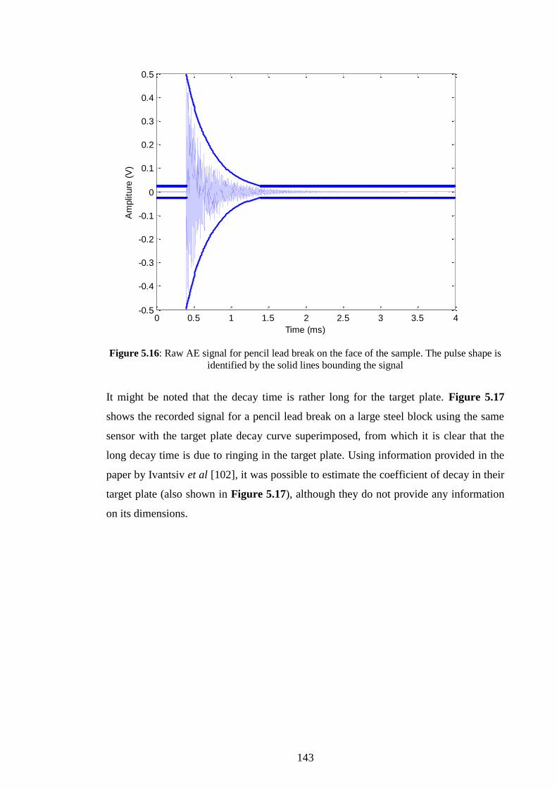
143

Figure 5.16: Raw AE signal for pencil lead break on the face of the sample. The pulse shape is

identified by the solid lines bounding the signal

It might be noted that the decay time is rather long for the target plate. Figure 5.17

shows the recorded signal for a pencil lead break on a large steel block using the same

sensor with the target plate decay curve superimposed, from which it is clear that the

long decay time is due to ringing in the target plate. Using information provided in the

paper by Ivantsiv et al [102], it was possible to estimate the coefficient of decay in their

target plate (also shown in Figure 5.17), although they do not provide any information

on its dimensions.

0 0.5 1 1.5 2 2.5 3 3.5 4-0.5

-0.4

-0.3

-0.2

-0.1

0

0.1

0.2

0.3

0.4

0.5

Time (ms)

Am

plit

ure

(V

)

144

Figure 5.17: Raw AE signal for pencil lead break on the face of a large cylindrical steel block.

Curve (a) is the decay curve estimated from Ivantsiv et al [102], and Curve (b) is the decay

curve for the target plate

The pulse shape function and the energy distribution p.d.f. can be used to simulate the

AE signal expected for any value of mass and nominal velocity, provided that the

particle arrival rate is known. After truncating the top 1% of the lognormal distribution,

it was then divided into 50 equal bins, whose individual integrals were computed and

multiplied by the total number of particles and divided by the energy of the bin to obtain

the corresponding number of particles in each bin. The AE energy associated with each

bin was converted to a voltage using Equation 5.5 and the corresponding pulses

generated from Equation 5.4 were distributed randomly within a simulated record,

assuming no medium-term fluctuation in the mass flow rate. Overlapping was dealt with

simply by adding the two pulse functions in a given interval. Figures 5.18 and 5.19

show two extremes of simulated time series records for a heavily overlapped and a

sparse signal respectively, alongside an example measured record with the non-noise

peaks labelled. As can be seen, the simulated signals have fewer peaks, since there are

no noise peaks, and allow a wider distribution of peak heights. Figure 5.20 shows

simulated and measured time series for one of the cases where it was not possible to

identify individual arrivals not only because of the strong degree of overlapping, but

also because of the low signal : noise. Also shown in Figure 5.20 is a simulation of the

0.4 0.45 0.5 0.55 0.6 0.65 0.7 0.75

-0.08

-0.06

-0.04

-0.02

0

0.02

0.04

0.06

0.08

0.1

Time (ms)

Am

plit

ure

(V

)( a )

( b )

145

effect of reducing the amount of ringing in the target plate, indicating how the

simulation can be used to design the sensing/acquisition approach and to determine

performance limits.

Figure 5.18: Measured (top) and simulated AE records for 212-250μm silica sand with nominal

impact velocity of 12.3 ms-1

, and particle arrival rate of 900 per second. Peaks that were

identified as particle impacts in the measured record are labelled

0.72 0.721 0.722 0.723 0.724 0.725 0.726 0.727 0.728 0.729 0.730

0.005

0.01

0.015

0.02

0.025

0.03

0.035

0.04

0.045

Am

plit

ude (

V)

Time (s)

0.72 0.721 0.722 0.723 0.724 0.725 0.726 0.727 0.728 0.729 0.730

0.01

0.02

0.03

0.04

0.05

0.06

Am

plit

ude (

V)

Time (s)

P1

P2

P3

P4

P5

P6P7

P8

146

Figure 5.19: Measured (top) and simulated AE records for 710-850μm glass beads with

nominal impact velocity of 4 ms-1

, and particle arrival rate of 40 per second. Peaks that were

identified as particle impacts in the measured record are labelled

Figure 5.20: Measured (top) and simulated AE records for 125-180 μm silica sand with


, and particle arrival rate of 4000 per second Simulations

with a decay constant of 3000sec-1

(middle) and 30000sec-1

(lower)

1.87 1.88 1.89 1.9 1.91 1.92 1.93 1.94 1.95 1.96 1.970

0.02

0.04

0.06

0.08

0.1

Am

plit

ude (

V)

Time (s)

1.87 1.88 1.89 1.9 1.91 1.92 1.93 1.94 1.95 1.96 1.970

0.01

0.02

0.03

0.04

0.05

0.06

0.07

0.08

0.09

0.1

Am

plit

ude (

V)

Time (s)

P1P2

P3

P4

1 1.001 1.002 1.003 1.004 1.005 1.006 1.007 1.008 1.009 1.010

0.01

0.02

0.03

0.04

0.05

Am

plit

ude (

V)

Time (s)

1 1.001 1.002 1.003 1.004 1.005 1.006 1.007 1.008 1.009 1.01

0.01

0.02

0.03

0.04

Am

plit

ude (

V)

Time (s)

1 1.001 1.002 1.003 1.004 1.005 1.006 1.007 1.008 1.009 1.010

0.01

0.02

0.03

0.04

Am

plit

ude (

V)

Time (s)

147

In order to evaluate the performance of the time series model, the energy of the

simulated AE time series signal was correlated to the energy of raw AE signal

(including the fraction 125-180 μm). Figure 5.21, shows that the average slope is very

close to unity, although there is a distinct tendency for small particle sizes to contain

about 10% excess energy in the simulation and larger particle sizes to show a 10%

deficit. The error for the larger particles is likely to be because of some noise leakage

into the correlated distributions whereas the excess for the smaller particles is likely to

be due some signal being lost in the noise for the correlated distributions. Overall, the

correlation shows that the model can be used to simulate time series where the degree of

overlap is such that individual particles cannot be resolved.

Figure 5.21: AE energy from simulated time series signal versus raw AE energy

y = 1.0246x

y = 0.9x

y = 1.1x

0

0.01

0.02

0.03

0.04

0.05

0.06

0.07

0.08

0 0.01 0.02 0.03 0.04 0.05 0.06 0.07 0.08

Raw signal AE energy (V2.s)

Sim

ula

ted

Sig

na

l A

E e

ne

rgy

(V2

.s)

125-180 μm

212-250 μm

300-425 μm

500-600 μm

600-710 μm

710-850 μm

148

Chapter 6

Analysis and Discussion

This chapter uses the findings of Chapter 5, in which it was demonstrated that an AE

time series could be simulated for dry particle impacts. Using this model, it is then

possible to analyse more meaningfully data which include cases where the particles act

as an ensemble. The approach is applied first to the remaining dry particle impact data,

then to the slurry impingement results and, finally, to the results for the flow loop.

6.1 Airborne particle impact test

The main aim of the dry impact study was to assess whether AE energy could be

calibrated for incident particle kinetic energy under a wide range of conditions where

particles could be relatively easily controlled. Figures 6.1 to 6.4 present all of the

measured data in a format that allows such an assessment, where the measured energy is

divided by particle mass (Figures 6.1 and 6.2) and by the square of particle velocity

(Figures 6.3 and 6.4).

As can be seen in Figures 6.1 and 6.2, AE energy per particle per unit mass generally

increases with increasing particle velocity across the whole range of mass and velocity

studied. However, the measured AE energy per particle per unit mass is higher for

individual impacts and shows a stronger dependence on particle velocity than that for

multiple impacts at higher velocities but the difference is less evident at lower

velocities. As the velocity increases, the number of particle impacts per second

increases from a few hundreds to a few thousands, and this may lead to overlapping of

the transmission paths, or, indeed, to particle interactions at or near the surface, both of

which would reduce the amount of energy being recorded at the sensor for each particle.

Closer inspection of Figure 6.2 also shows that the lower fractions of the low mass

range and high mass range (1a vs 1b and 3 vs 4) for single impacts both exhibit higher

energies per unit mass, whereas this is not observed for multiple impacts. For the

smaller particles, this might be explained by the difficulty in controlling the number of

particles leaving the shaker, where perhaps more than one is recorded on some

occasions. The particle streams, where relatively large numbers of particles impinge on

149

the surface, would not be susceptible to this type of error. This explanation does not

hold for the high mass particles which are large enough to be individually handled, and

here the explanation is more likely to be that the particle momentum is sufficient to

cause significant whole body movement of the target (specimen and holder) and hence a

different additional energy dissipation mechanism.

Figure 6.1 AE energy per unit mass versus particle velocity for all regimes investigated: (A)

low velocity, (5) high velocity-low mass single impacts, (6) high velocity-low mass multiple

impacts

Figure 6.2: AE energy per unit mass versus particle velocity for all low velocity measurements

(area A above): (1a) low mass-lower range single impacts, (1b) low mass-higher range single

impacts, (2) low mass multiple impacts, (3) high mass-lower range, (4) high mass-higher range

0

100000

200000

300000

400000

500000

600000

700000

800000

900000

1000000

0 2 4 6 8 10 12 14 16 18

Particle velocity, ms -1

AE

en

erg

y/p

art

icle

/un

it m

ass, V

2sec/g

5

6

A

0

5000

10000

15000

20000

25000

30000

0.5 1 1.5 2 2.5 3


AE

en

erg

y/p

art

icle

/un

it m

as

s,

V2s

ec

/g

1b

2

3

4

1a

150

Figure 6.3 shows that AE energy per particle divided by the square of the velocity

increases with particle diameter only up to a diameter of about 1.5mm, above which the

energy appears to remain constant. Figure 6.3 also shows that the curvature at

diameters less than 1.5mm is positive, ie. a higher order dependence than linear. The AE

energy level is again higher for single impacts than for multiple impacts at high

velocities (5 vs 6) and not at low velocities (2 vs 1) attributable, again, to the

overlapping effect described above.

Figure 6.3: AE energy per particle divided by the square of the velocity versus particle diameter

for all regimes investigated: (B) low velocity-low mass regime, (3) high mass-lower range, (4)

high mass-higher range, (5) high velocity-low mass single impacts, (6) high velocity-low mass

multiple impacts

0

25

50

75

0 1000 2000 3000 4000 5000

AE

en

erg

y/p

art

icle

/sq

ua

re v

elo

cit

y,

V2 s

ec/m

2s

-2

Mean particle diameter, μm

3

4

5

6

B

151

Figure 6.4: AE energy per particle divided by the square of the velocity versus particle diameter

for low velocity-low mass regime (area B above): (1) low velocity-low mass single impacts, (2)

low velocity-low mass multiple impacts

Since there is a clearly different mechanism of energy dissipation occurring at

diameters greater than 1.5mm, these data were excluded when determining the velocity

and diameter exponents, and the relevant plots are shown in Figures 6.5 and 6.6.

As can be seen from Figure 6.5, the velocity exponent is very close to 2 when taking all

the data together, although it might be noted that there are two reasonable distinct sets

of points, the single impacts, where the exponent is about 2.3 and the multiple impacts

where the exponent was around 1.5. This is in accord with the findings of Feng and Ball

[13], who observed a diameter exponent of 3 and a velocity exponent which varied

between 1.1 and 3.4. It therefore appears that, when the particles approach the surface

individually, their impact velocity is reasonably predictable, whereas, if there is a

stream, interactions within the stream and at, or near the surface, may well affect the

actual impingement velocity (magnitude and direction) for each particle. Deng et al

[63], for example, have found, for an average velocity of about 20 m/s, that actual

particle velocities at the outlet of the acceleration tube varied from 6 m/s up to 30 m/s.

Moreover, Shipway and Hutchings [56] have suggested that the particles in the

acceleration tube are subject to many impacts between themselves and with the wall of

the nozzle as they are accelerated, and that such impacts will tend to reduce the final

velocity.

0

0.1

0.2

0.3

0.4

0.5

0.6

0.7

0.8

0.9

1

0 100 200 300 400 500 600

AE

en

erg

y/p

art

icle

/sq

ua

re v

elo

cit

y,

V2 s

ec/m

2s

-2


2

1

152

Figure 6.5: The dependence of AE energy per unit mass upon particle velocity

Figure 6.6, shows that, assuming that the velocity exponent is 2, particle diameter

exponent is close to 3, which is in agreement with other workers [23, 73]. Figure 6.6

does reveal, however, that particles of diameter greater than about 1mm lie above the

best-fit curve (and therefore contribute to the exponent being a little above 3). This

might be an effect of the experimental conditions since these particles are large enough

to handle and observe easily, and hence their velocities may be more tightly controlled,

and/or because none of these larger particles were used in multiple impact streams.

In summary, this analysis shows that, within the range of experimental error, the natural

variations of particle size, and possible effects of overlap and interactions, airborne

particle impacts generate AE energy that is approximately proportional to

, i.e. the total kinetic energy. Taking account of the variation in

particle mass and comparing calculated with observed distributions of AE event energy

confirms this approach and justifies the summation even when the events cannot be

distinguished. The approach, however, only holds for particle diameters below about 1

mm, after which a different energy dissipation mechanism appears to be operating.

y = 4972.5x2.3484

y = 7248.1x1.5285

y = 5207.2x2.0754

0

500000

1000000

1500000

2000000

2500000

3000000

3500000

0 2 4 6 8 10 12 14 16 18


AE

en

erg

y/p

art

icle

/un

it m

ass,

V2sec/g

single impact regimes

multiple impact regimes

All regimes

153

Figure 6.6: Influence of mean particle diameter on AE energy divided by the square of impact

velocity

6.2 Slurry jet impingement

The purpose of this section is to extend the applicability of the statistical model

described in Chapter 5 to relatively uncontrolled impingement experiments where the

carrier fluid was a liquid as well as to assess the extent to which the previous findings

can be applied with this medium. Emphasis is placed on the effect of fluid mechanical

phenomena on the motion of particles near the target, applied first to a free jet in the

interest of comparison with experiments with a free air jet.

Given that the measured AE energy shows roughly the expected variation with speed,

particle density, nominal impact angle and particle size, as shown in Section 4.2, it

remains to be seen whether the energy measured corresponds to what would be

expected from the log-normal distribution function developed in Chapter 5 to describe

the probability distribution of particle arrival AE energy for air-propelled particles using

the same target and sensor. The mean of this distribution was found to vary with

particle arrival speed, and the correlation between the mean AE energy determined for

the dry impacts is reassessed first, based on the smaller particle size ranges (300-425

µm and 212-250 µm) used in the slurry impingement tests. Figure 6.7 shows the best fit

y = 2E-09x3.2157

R2 = 0.831

0

20

40

60

80

100

120

0 200 400 600 800 1000 1200 1400 1600


AE

en

erg

y/p

art

icle

/sq

uare

velo

cit

y,

V2sec/m

2s-2

154

mean along with error bars indicating the range of values over the five observations for

each incident energy giving the mean AE energy:

(6.1)

Figure 6.7: Correlation between the mean of the lognormal distribution and nominal incident

energy, using data from Figure 5.12

The expected AE energy in a population of impacts, Ecalculated , can now be obtained

using the average particle arrival rate given in Table 3.7 and the mean of the energy

distribution function:

(6.2)

The measured AE energy associated with the particles, Emeasured , can be estimated by

subtracting the background water jet energy Ew from the integral of the signal, E:

where Ew was taken as the average of the three curves shown in Figure 3.28.

Emean= 2.8639mVp2

R² = 0.62

0.0E+00

5.0E-06

1.0E-05

1.5E-05

2.0E-05

2.5E-05

3.0E-05

3.5E-05

4.0E-05

4.5E-05

0.E+00 2.E-06 4.E-06 6.E-06 8.E-06 1.E-05 1.E-05

Mean

of

p.d

.f, E

me

an

mVp2 ( J )

(6.3)

155

The nominal impact angle is accounted for by calculating the normal component of the

jet exit velocity, and Figure 6.8 shows the resulting relationship between the measured

and calculated energy and, as can be seen, there is a considerable discrepancy between

(measured) wet and (calculated) dry impacts with the same jet exit velocity, the dry

impacts giving at least a factor 10 higher AE energy. Such a discrepancy in the AE

energy could stem from the difference in the carrier medium and its influence on the

direction of particles. For particles laden gases, this direction is little affected by the

spreading effect of the fluid, because the viscosity of air is very small (1.81×10-5

Kg.m-1

sec-1

), leading to a much lower drag force than arises from the viscosity of a

water-based carrier (8.9×10-4

Kg.m-1

sec-1

). Therefore, the incident particle velocity is

important, but there are difficulties in measuring or modelling this.

Figure 6.8: Measured and calculated AE energy, assuming the particle arrival speeds given in

Table 3.7

The most likely reason for the discrepancy in Figure 6.8 is that the water-driven

particles are moving much less rapidly than the jet exit velocity when they strike the

target. To deal with this, the empirical model of Turrene and Fiset [94] (Equation 2.13)

was used to calculate the average arrival speed, using the particle mean diameter, the jet

exit velocity, and taking an average value of the initial radial position of the particle

(1.25mm). Table 6.1 shows the calculated arrival speeds for all the conditions studied.

In some cases of slowly moving particles the model does not give a positive speed,

corresponding to particles that fail to penetrate the squeeze film.

0

1

2

3

4

5

6

7

8

0 0.05 0.1 0.15 0.2

Cal

cula

ted

AE

en

erg

y, V

2 se

c

Measured AE energy, V2sec

156

Particle size range (µm) Jet exit velocity (m/s) Average calculated arrival speed

(m/s)

125-180

4.2 -

6.8 0.21

10.2 0.73

12.7 1.10

212-250

4.2 -

6.8 0.30

10.2 0.95

12.7 1.43

300-425

4.2 0.10

6.8 0.84

10.2 1.80

12.7 2.50


Figures 6.9 to 6.11 show the calculated and measured AE energy for each of the three

impact angles, sorted for each of the particle sizes, and using the estimated impact speed

following Turenne and Fiset. As can be seen, the calculated and measured values are

much more compatible, the slope varying from a little below unity to a little above and

these are listed in Table 6.2 along with the average slope for each angle. Figure 6.12

shows that the average slope is very close to unity when taking all the data together,

although there is a distinct tendency for smaller particles to have higher than expected

energy and larger particles to have lower than expected. Table 6.2 also shows the

average slope to be very close to unity for nominal impact angles of 60o and 90

o, but

rather less for impingement at 30o, even when the normal component is taken into

account.

The particle size effect might be explained by the fact that the slurry jet is directed

horizontally, so that there might be some drop-out relative to the water which would

change the angle and also proportion of particles striking the surface, and this would

affect larger particles more than smaller ones. Also, streams that are directed in a

downward direction will have the vertical (parallel to the target) component of their

velocity affected more than the horizontal, and so the lower impingement angles might

157

be expected to have lower normal speeds than expected, and this would be expected to

affect the larger particles more.

Figure 6.9: Calculated AE energy versus measured AE energy at nominal impact angle 90o


Ec= 1.5Em R² = 0.585

Ec = 0.8Em R² = 0.7755

Ec= 0.6Em R² = 0.8019

0.00

0.02

0.04

0.06

0.08

0.10

0.12

0.14

0.16

0.18

0.20

0.00 0.05 0.10 0.15 0.20

Cal

cula

ted

AE

en

rgy,

V2 s

ec


125-180

212-250

300-425

Ec= 1.4Em R² = 0.57

Ec= 0.85Em R² = 0.71

Ec= 0.63Em R² = 0.69

0.00

0.01

0.02

0.03

0.04

0.05

0.06

0.07

0.08

0.09

0.10

0.00 0.02 0.04 0.06 0.08 0.10 0.12

Cal

cula

ted

AE

en

rgy,

V2se

c


125-180

212-250

300-425

158


Nominal impact

angle (θo)

Particle size range

(µm) Correlation function Average slope

90

125-180 Ec=1.53 Em

0.99 212-250 Ec=0.82 Em

300-425 Ec =0.63 Em

60

125-180 Ec =1.39 Em

0.95 212-250 Ec =0.85 Em

300-425 Ec=0.63 Em

30

125-180 Ec =0.85 Em

0.61 212-250 Ec =0.40 Em

300-425 Ec =0.60 Em

Table 6.2: summary of correlation functions between calculated and measured AE energy

Ec= 0.85Em R² = 0.535 Ec= 0.4Em

R² = 0.8714

Ec= 0.6Em R² = 0.826

0.00

0.01

0.02

0.03

0.04

0.05

0.06

0.07

0.00 0.02 0.04 0.06 0.08

Cal

cula

ted

AE

en

erg

y, V

2 se

c


125-180

212-250

300-425

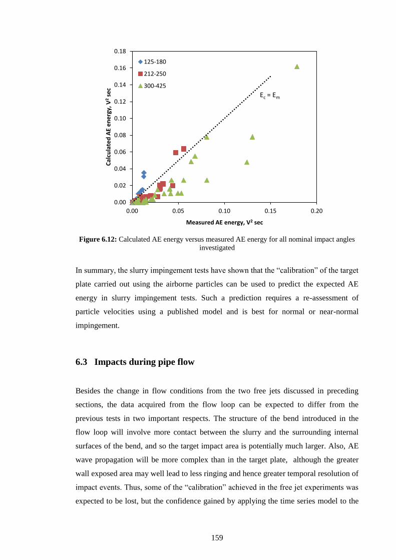
159

Figure 6.12: Calculated AE energy versus measured AE energy for all nominal impact angles

investigated

In summary, the slurry impingement tests have shown that the “calibration” of the target

plate carried out using the airborne particles can be used to predict the expected AE

energy in slurry impingement tests. Such a prediction requires a re-assessment of

particle velocities using a published model and is best for normal or near-normal

impingement.

6.3 Impacts during pipe flow

Besides the change in flow conditions from the two free jets discussed in preceding

sections, the data acquired from the flow loop can be expected to differ from the

previous tests in two important respects. The structure of the bend introduced in the

flow loop will involve more contact between the slurry and the surrounding internal

surfaces of the bend, and so the target impact area is potentially much larger. Also, AE

wave propagation will be more complex than in the target plate, although the greater

wall exposed area may well lead to less ringing and hence greater temporal resolution of

impact events. Thus, some of the “calibration” achieved in the free jet experiments was

expected to be lost, but the confidence gained by applying the time series model to the

0.00

0.02

0.04

0.06

0.08

0.10

0.12

0.14

0.16

0.18

0.00 0.05 0.10 0.15 0.20

Cal

cula

ted

AE

en

erg

y, V

2 se

c

Measured AE energy, V2 sec

125-180

212-250

300-425

Ec = Em

160

free jet experiments was expected to allow an assessment of the factors which need to

be taken into account in a real implementation.

This section firstly presents a more detailed analysis of the particle-free water AE

signals in order to identify the background noise characteristics, and hence develop a

model for background water noise which is itself more complex than for the slurry jet.

Then, the analysis was focused onto dividing the AE recorded in particle-laden flows

into stationary and non-stationary parts and dealing with the non-stationary part where

frequency can vary substantially with time.

6.3.1 Analysis for particle-free water

The high AE energy associated with the water impingement signal in the flow loop

dictated a different approach to that used in slurry impingement, where it was possible

simply to subtract an average energy. In particular, the hydraulic conditions produce a

strong pulsatile nature to the particle-free time series which can be seen as a carrier

wave for the particle signatures. Dealing with such pulsatile signals requires a

demodulated analysis of the signals to make use of the periodicity.

Figure 6.13 shows samples of typical raw AE signals recorded for water impingement

along with typical raw AE spectra over the range of flow speeds tested. It is clear that

the raw AE signal amplitude, in general, increases with increasing flow speed. The

effect of the sensor bandwidth is apparent in the raw frequency spectrum, with most

energy being contained in the range 100-400 kHz. The spectra show that most of the

power is focused in three bands; one very narrow band centred on a frequency of around

100 kHz and characterised by a spike at the lowest speed whose magnitude decreases

rapidly with increasing flow speed, a band at 150 kHz to 200 kHz, and another band at

300 kHz to 400 kHz. It is also clear that, within its bandwidth, the sensor shows a

systematic shift in frequency content (power) towards the higher end as the flow speed

increases. To quantify these systematic changes in raw AE frequency content, the

proportion of the total energy in these three frequency bands was determined, for each

of the 20 AE records at each flow speed. Figure 6.14 shows the variation in AE energy

proportion in each band with flow speed where each point represents the average of 20

AE records along with the standard deviation. As can be seen, the first band decreases

rapidly with flow speed while the highest frequency increases with speed. Thus, raw AE

frequency analysis can potentially offer a means of monitoring flow speed.

161

Raw AE signal Frequency spectrum

(a)

(b)

(c)

(d)

Figure 6.13: Typical 1-second raw AE time series for water impingement in the flow loop and

their corresponding raw frequency spectra for flow speeds: (a) 4.2 ms-1

, (b) 6.8 ms-1

, (c) 10.2

ms-1

, and (d) 12.7 ms-1

0 0.1 0.2 0.3 0.4 0.5 0.6 0.7 0.8 0.9 1-0.04

-0.03

-0.02

-0.01

0

0.01

0.02

0.03

Time (s)

Am

plit

ure

(V

)

0 1 2 3 4 5 6 7 8 9 10

x 105

0

0.2

0.4

0.6

0.8

1

1.2

1.4

1.6

1.8x 10

-8

Frequency (Hz)

Pow

er

spectr

al density

0 0.1 0.2 0.3 0.4 0.5 0.6 0.7 0.8 0.9 1-0.4

-0.3

-0.2

-0.1

0

0.1

0.2

0.3

Time (s)

Am

plitu

re (

V)

0 1 2 3 4 5 6 7 8 9 10

x 105

0

0.5

1

1.5

2

2.5

3

3.5

4

4.5

5x 10

-9

Frequency (Hz)

Pow

er

spectr

al density

0 0.1 0.2 0.3 0.4 0.5 0.6 0.7 0.8 0.9 1-0.8

-0.6

-0.4

-0.2

0

0.2

0.4

0.6

Time (s)

Am

plitu

re (

V)

0 1 2 3 4 5 6 7 8 9 10

x 105

0

0.2

0.4

0.6

0.8

1

1.2

1.4x 10

-8

Frequency (Hz)

Pow

er

spectr

al density

0 0.1 0.2 0.3 0.4 0.5 0.6 0.7 0.8 0.9 1-0.8

-0.6

-0.4

-0.2

0

0.2

0.4

0.6

0.8

Time (s)

Am

plitu

re (

V)

0 1 2 3 4 5 6 7 8 9 10

x 105

0

1

2

3

4

5

6

7x 10

-8

Frequency (Hz)

Pow

er

spectr

al density

162

Figure 6.14: Proportion of AE energy in raw frequency bands versus flow speed; Band 1: 100

kHz, Band 2: 150-200 kHz, Band 3: 300-400 kHz

Figure 6.15 shows a magnified 0.1-second segment of the record depicted in

Figure 6.13a in both raw and averaged forms. These signals suggest a strong influence

of fluid pulses on the recorded AE with a pulse period of around 0.01 s, most likely

associated with the rotational speed of the pump.

(a) Raw AE signal (b) RMS AE signal

Figure 6.15: Magnified view of 0.1-second segment of the signal shown in Figure 6.13a,

(a) raw and (b) RMS AE

To investigate the lower frequency characteristics of the water impingement signals,

demodulated frequency analysis was applied to all signals at all flow speeds tested.

First, the raw AE signals were averaged with a 0.2 ms averaging time (over 500 points)

using a root mean square (RMS) algorithm, making the effective sampling rate 5000 Hz

samples per second as shown in Figure 6.15b. Then, the RMS AE signal was made

0

0.2

0.4

0.6

0.8

1

1.2

0 2 4 6 8 10 12 14

Pro

po

rtio

n o

f e

ne

rgy

Flow speed, m/s

Band 1

Band 2

Band 3

0 0.01 0.02 0.03 0.04 0.05 0.06 0.07 0.08 0.09 0.1-0.025

-0.02

-0.015

-0.01

-0.005

0

0.005

0.01

0.015

0.02

0.025

Time (s)

Am

plit

ure

(V

)

0 0.01 0.02 0.03 0.04 0.05 0.06 0.07 0.08 0.09 0.10

0.002

0.004

0.006

0.008

0.01

0.012

0.014

Am

plit

ude (

V)

Time (s)

163

bipolar by subtracting the mean value of the record from each point in order to remove

the DC component before transforming the signal into the frequency domain. Finally,

all spectra were normalized to a unit energy content in order to facilitate comparison.

Figure 6.16 shows typical examples of the resulting normalized RMS AE signals along

with the corresponding normalized frequency for water impingement for each of the

flow speeds tested. The frequency domain at the lowest flow speed, Figure 6.16a,

shows spectral peaks occurring at relatively regular frequency intervals which imply the

possibility of one fundamental frequency component with other peaks resulting from

harmonics. On closer inspection, it was found that two spectral peaks are dominant; 100

Hz at the lowest flow speed and 42 Hz at the highest flow speed, Figure 6.16d.

Between the two extreme speeds, the energy in the 100 Hz peak decreases with speed

while the 42 Hz increases. The spectra at the intermediate speeds show a transition

between the two extremes, Figure 6.16b showing both spectral peaks and Figure 6.16c

exhibiting a broad demodulated frequency spectrum.

At first sight, the complexity of what is essentially a noise pattern might make the

identification of particle impact signatures a daunting prospect. However, a clear

understanding of this pattern assists in separating signal from noise, but also allows the

exploration of the potential to use the low frequency as a carrier wave.

164

RMS AE signal Normalized Frequency spectrum

(a)

(b)

(c)

(d)

Figure 6.16: Typical 1-second RMS AE signals for water impact and their corresponding

normalized demodulated spectrum for flow speeds: (a) 4.2 ms-1

, (b) 6.8 ms-1

, (c) 10.2 ms-1

, and

(d) 12.7 ms-1

0 0.1 0.2 0.3 0.4 0.5 0.6 0.7 0.8 0.9 1-6

-4

-2

0

2

4

6x 10

-3

Am

plitu

de (

V)

Time (s)

0 500 1000 1500 2000 25000

0.02

0.04

0.06

0.08

0.1

0.12

0.14

0.16

Frequency (Hz)

Pow

er s

pect

ral d

ensi

ty

0 0.1 0.2 0.3 0.4 0.5 0.6 0.7 0.8 0.9 1-0.01

0

0.01

0.02

0.03

0.04

0.05

0.06

0.07

0.08

Am

plitu

de (

V)

Time (s)0 500 1000 1500 2000 2500

0

0.005

0.01

0.015

0.02

0.025

Frequency (Hz)

Pow

er s

pect

ral d

ensi

ty

0 0.1 0.2 0.3 0.4 0.5 0.6 0.7 0.8 0.9 1-0.02

0

0.02

0.04

0.06

0.08

0.1

0.12

0.14

0.16

Am

plitu

de (

V)

Time (s)

0 500 1000 1500 2000 2500

0.5

1

1.5

2

2.5

3x 10

-3

Frequency (Hz)

Pow

er s

pect

ral d

ensi

ty

0 0.1 0.2 0.3 0.4 0.5 0.6 0.7 0.8 0.9 1-0.05

0

0.05

0.1

0.15

0.2

Am

plitu

de (

V)

Time (s)

0 500 1000 1500 2000 25000

1

2

3

4

5

6

7

8x 10

-3

Frequency (Hz)

Pow

er s

pect

ral d

ensi

ty

165

In order to quantify these demodulated spectra, a processing approach was devised

based on categorisation of peak heights and their corresponding frequencies. For each

flow rate, across the 20 records, all peaks in the spectrum were identified automatically

by first applying an identification threshold of 5% the maximum peak heights and then

obtaining each peak height and its corresponding frequency. The ten highest peaks in

the spectrum were then taken along with their corresponding frequency values for each

record. Next, the resulting 200 values of peak height and corresponding frequency for

each combination were used as an input to a Matlab algorithm. The algorithm divided

the frequency range into 20 Hz bins and allocated each peak height to the appropriate

frequency bin, calculating the number of occurrences in each bin. The average peak

height for each bin was then determined by dividing the sum of all peak heights by the

number of occurences: . Figure 6.17

summarises the results, quantifying the two distinct frequency patterns described above.

As can be seen in Figure 6.17a a very clear harmonic pattern occurs at low speed with a

fundemantal frequency of 100 Hz and charactersied by a set of much smaller harmonics.

At the next highest speed, Figure 6.17b a broader spectrum based on 42 Hz begins to

emerge alongside the 100 Hz pattern noted in Figure 6.17a. At the highest speed, the

100 Hz pattern is absent and is replaced by the 42 Hz band plus some higher frequency

components not on the 100 Hz series. The spectrum for the higher intermediate speed is

slightly anomalous in that, although it contains a growing 42 Hz component, there are a

number of other components present at higher intensity. Although the exact causes of

this low frequency spectral behaviours are not entirely clear, it is likely that they are

associated with the hydraulic behaviour of the flow loop. The rotational speed of the

pump is 10 Hz, so this does not explain either the 42 Hz or 100 Hz frequencies, nor,

indeed the very obvious pulsation at lower speed. In fact, the spiral shape of the mono

pump impeller is specifically designed to eliminate flow pulsations. However, it is

possible that any practical application will be on a system with its own hydraulic

characteristics, so the flow loop provides an example of how such characteristics might

be dealt with in attempting to monitor particle impingement.

166

0 100 200 300 400 500 6000

0.02

0.04

0.06

0.08

0.1

0.12

0.14

0.16

Peak h

eig

ht

(Arb

itra

ry U

nits)

Frequency (Hz)

0 100 200 300 400 500 6000

0.002

0.004

0.006

0.008

0.01

0.012

0.014

0.016

0.018

0.02

Pea

k he

ight

(Arb

itrar

y U

nits

)

Frequency (Hz)

42 Hz

(b)

(a)

167

Figure 6.17: Distribution of the ten top frequency peak heights for water impingement at four

flow speeds: (a) 4.2 ms-1

, (b) 6.8 ms-1

, (c) 10.2 ms-1

, and (d) 12.7 ms-1

The proportion of oscillatory energy that is contained in the top 10 peaks for all flow

speeds is shown in Figure 6.18. As can be seen, the remaining energy is quite high for

the higher speeds indicating a generally more broadband distribution of energy.

0 100 200 300 400 500 6000

0.5

1

1.5

2

2.5x 10

-3

Pea

k he

ight

(Arb

itrar

y U

nits

)

Frequency (Hz)

42 Hz

0 100 200 300 400 500 6000

1

2

3

4

5

6x 10

-3

Pea

k he

ight

(Arb

itrar

y U

nits

)

Frequency (Hz)

42 Hz

(c)

(d)

168

Figure 6.18: Proportion of the oscillatory energy contained in the top 10 peaks for water

impingement at four flow speeds: (a) 4.2 ms-1

, (b) 6.8 ms-1

, (c) 10.2 ms-1

, (d) 12.7 ms-1

Considering only the total AE energy analysis is not sufficient for practical situation,

and bearing in mind the fact that the signal is not wholly continuous which indicates a

dynamic effect which potentially contains information below and above the mean

energy level, the total AE energy for slurry impingement signal was divided into static

and oscillated parts.

As is obvious from the foregoing, any model for the AE arising from water

impingement will consist of an oscillatory component and a static component.

Therefore the total AE energy was divided into two parts, a static component Est and an

oscillatory component Eosc. The static component was simply obtained by calculating

the average of the entire AE record. The oscillatory part was obtained by integrating the

RMS of the 1-second averaged records using Equation (3.1), once the static component

had been removed (records such as those shown in Figure 6.16).

Figures 6.19 and 6.20 show the effect of flow speed on both the static and dynamic AE

energy components, respectively. Since there is no particular reason to expect the

hydraulic behaviour to show a power law dependence with flow speed, an exponential

0 100 200 300 400 500 6000

0.1

0.2

0.3

0.4

0.5

0.6

0.7

0.8

Energ

y p

roport

ion

Frequency (Hz)

0 100 200 300 400 500 6000

0.1

0.2

0.3

0.4

0.5

0.6

0.7

Energ

y p

roport

ion

Frequency (Hz)

0 100 200 300 400 500 6000

0.005

0.01

0.015

0.02

0.025

0.03

0.035

0.04

Energ

y p

roport

ion

Frequency (Hz)

0 100 200 300 400 500 6000

0.01

0.02

0.03

0.04

0.05

0.06

0.07

0.08

0.09

0.1

Energ

y p

roport

ion

Frequency (Hz)

(a) (b)

(c) (d)

169

fit showing the dependence of AE energy components associated with (v-4.1) was used

in the interest of obtaining a better fit, although the best fit power equation is also

shown for each AE component. Thus, the AE energy associated with water

impingement can be described by a mean level and

an oscillatory component of energy .

Figure 6.19: Effect of flow speed on static AE energy for water impingement showing the best

power fit and the best exponential fit

Figure 6.20: Effect of flow speed on oscillatory AE energy for water impingement showing the

best power fit and the best exponential fit

Estw = 0.0013e0.29(v-4.1)

R² = 0.9454

Estw = 0.0035(v-4.1)0.4205

R² = 0.6041

0

0.002

0.004

0.006

0.008

0.01

0.012

0.014

0.016

0.018

0 2 4 6 8 10

Stat

ic A

E e

ne

rgy,

Est

w, V

2 se

c

Flow speed, (v-4.1), m/s

Eoscw = 0.0026e0.19(v-4.1)

R² = 0.8199

Eoscw = 0.0052(v-4.1)0.24

R² = 0.3911

0

0.002

0.004

0.006

0.008

0.01

0.012

0.014

0.016

0.018

0.02

0 2 4 6 8 10

Osc

illat

ed

AE

en

erg

y, E

osc

w, V

2se

c

Flow speed, (v-4.1), m/s

170

6.3.2 Slurry impact analysis

A similar decomposition into static and oscillatory components (Figure 6.21) was used

to analyse the AE from a particle-laden flow. The first stage in the analysis of particle-

laden flow was to separate the two main components of the signal in a systematic way.

To do so, the total AE energy for each record, was divided into its two main

components the static component, and the oscillatory component, in the same

way as was done for particle-free water. Each of these can be further divided

accordingly into components due to particles Ep and due to water E

w.

The static energy associated with particle impact, , can be determined by subtracting

the actual average values of the static energy of water impingement Figure 6.19, ,

from the total static energy of the slurry as: .

Figure 6.21: Schematic illustration of the decomposition of slurry impingement AE energy in

the flow loop

Figures 6.22 to 6.25 show the effect of flow speed on the static AE energy associated

with particle impacts for all particle sizes and nominal concentrations tested. As before,

the best power law fit was used and the resulting exponents are shown in Table 6.3.

Total energy:

Esltot

Total static energy componenent:

Esl st

Static energy for water impingement:

Ew st

Static energy for particle impact:

Ep st

Total oscillatory energy component:

Esl osc

Oscillatory energy for 100 Hz harmonic

series

Esl sp1

Oscillatory energy for 42 Hz band

Esl sp2

Remaining energy in the demodulated

band

Esl broad

171

Figure 6.22: Effect of flow speed on the static AE energy for the three concentrations for

particles in size range 212-250 µm





0

0.002

0.004

0.006

0.008

0.01

0.012

0.014

0.016

0.018

0 2 4 6 8 10 12 14

Stat

ic A

E e

ne

rgy,

Est

p, V

2 se

c

Flow speed, v, m/s

C=1%

C=2.5%

C=5%

0

0.01

0.02

0.03

0.04

0.05

0.06

0.07

0.08

0.09

0 2 4 6 8 10 12 14

Stat

ic A

E e

ne

rgy,

Est

p, V

2se

c

Flow speed, v, m/s

C=1%

C=2.5%

C=5%

0

0.02

0.04

0.06

0.08

0.1

0.12

0 2 4 6 8 10 12 14

Stat

ic A

E e

ne

rgy,

Est

p, V

2 se

c

Flow speed, v, m/s

C=1%

C=2.5%

C=5%

172



Particle size range

(µm) Nominal concentration (kg/m

3)

Flow speed exponent

(n)

Curve fitting R2

value (%)

212-250

1 1.18 75

2.5 1.22 82

5 1.03 93

300-425

1 2.6 93

2.5 1.8 97

5 1.95 93

500-600

1 2.1 78

2.5 2.2 86

5 2.3 87

600-710

1 3.6 89

2.5 2.2 99

5 2.5 99

Table 6.3: Exponent of flow speed dependence of the static component of measured AE energy

for all flow loop tests

0

0.02

0.04

0.06

0.08

0.1

0.12

0.14

0.16

0 2 4 6 8 10 12 14

Stat

ic A

E e

ne

rgy,

Est

p, V

2 se

c

Flow speed, v, m/s

C=1%

C=2.5%

C=5%

173

In order to examine if the energy for slurry impingement is carried in the same

frequency bands as water impact, the dynamic slurry energy, was divided into three

parts, the component associated with the 100 Hz harmonic series, , the component

associated with the 42 Hz band, , and the remainder of the demodulated band

(see Figure 6.21),

(6.4)

To decompose the oscillatory part of the AE, each record was band-pass filtered twice

in the sp1 and sp2 bands using an infinite impulse response (IIR) digital filter of

Chebyshev Type I , set with a fifth order low pass digital Chebychev filter and 0.9 peak

to peak ripple in the bassband.

Figures 6.26 to 6.28 show the variation of the energy in each spectral component with

flow speed for all particle size fractions and solid concentrations tested, along with the

corresponding components for particle-free water. Over the range of flow speed, the

dominant band is the broad oscillatory component, the 100 Hz band only being

significant at lower flow speeds. The 42 Hz spectral component is always very small

and increases with flow speed. There is particularly no difference between the various

particle sizes and concentrations and particle-free water for this component, so it is of

little use in detecting particle impacts. Unlike all the other spectral components, the

100 Hz band decreases with flow speed. Figure 6.29 shows the effect of particle size

and concentration on this spectral component at the lowest flow speed. As can be seen,

the 100 Hz spectral component decreases with both the nominal particle concentration

and particle size range indicating that the pump rotational speed effect on the AE

recorded can be obscured by more particles in the mixture or bigger particle size range.

174

Figure 6.26: Effect of flow speed on the spectral AE energy, Esp1 , for the three concentrations

and particle-free water for each of the particle size ranges shown

0

0.001

0.002

0.003

0.004

0 2 4 6 8 10 12 14

Sp

ect

ral e

ne

rgy,

Esp

1,

V2 s

ec

Flow Speed, v, ms-1

water C=1% C=2.5% C=5%

dp=212-250 µm

0

0.0005

0.001

0.0015

0.002

0.0025

0.003

0.0035

0 2 4 6 8 10 12 14

Spe

ctra

l en

erg

y, E

sp1,

V

2se

c

Flow Speed, v, ms-1

water C=1% C=2.5% C=5%

dp=300-425 µm

0

0.0005

0.001

0.0015

0.002

0.0025

0.003

0.0035

0 2 4 6 8 10 12 14

Spe

ctra

l en

erg

y, E

sp1,

V

2se

c

Flow Speed, v, ms-1

water C=1% C=2.5% C=5%

dp=500-600 µm

0

0.0005

0.001

0.0015

0.002

0.0025

0.003

0.0035

0 2 4 6 8 10 12 14

Spe

ctra

l en

erg

y, E

sp1,

V

2 se

c

Flow Speed, v, ms-1

water C=1% C=2.5% C=5%

dp=600-710 µm

175

Figure 6.27: Effect of flow speed on the spectral AE energy, Esp2, for the three concentrations

and particle-free water for each of the particle size ranges shown

0.E+00

2.E-04

4.E-04

6.E-04

8.E-04

0 2 4 6 8 10 12 14

Sp

ect

ral e

ne

rgy,

Esp

2,

V2 s

ec

Flow Speed, v, ms-1

water, n=3.2 C=1%, n=2.4 C=2.5%, n=3.5 C=5%, n=3.3

dp=212-250 µm

0.E+00

2.E-04

4.E-04

6.E-04

8.E-04

0 2 4 6 8 10 12 14

Spe

ctra

l en

erg

y, E

sp2,

V

2 se

c

Flow Speed, v, ms-1

water, n=3.2 C=1%, n=3.2 C=2.5%, n=3.2 C=5%, n=2.4

dp=300-425 µm

0.E+00

2.E-04

4.E-04

6.E-04

8.E-04

0 2 4 6 8 10 12 14

Spe

ctra

l en

erg

y, E

sp2,

V

2se

c

Flow Speed, v, ms-1

water, n=3.2 C=1%, n=2.8 C=2.5%, n=3.1 C=5%, n=2

dp=500-600 µm

0.E+00

2.E-04

4.E-04

6.E-04

8.E-04

1.E-03

0 2 4 6 8 10 12 14

Spe

ctra

l en

erg

y, E

sp2,

V

2 se

c

Flow Speed, v, ms-1

water, n=3.2 C=1%, n=2.7 C=2.5%, n=2.7 C=5%, n=2

dp=600-710 µm

176

Figure 6.28: Effect of flow speed on the broad spectral AE energy, Ebroad, for the three

concentrations and particle-free water for each of the particle size ranges shown

0

0.005

0.01

0.015

0.02

0 2 4 6 8 10 12 14

Bro

ad s

pe

ctra

l en

erg

y,

E bro

ad ,

V2 s

ec

Flow Speed, v, ms-1

water, n=3.6 C=1%, n=2.3 C=2.5%, n=3.1 C=5%, n=2.7

dp=212-250 µm

0

0.005

0.01

0.015

0.02

0 2 4 6 8 10 12 14

Bro

ad s

pe

ctra

l en

erg

y,

E bro

ad ,

V2 s

ec

Flow Speed, v, ms-1

water, n=3.6 C=1%, n=2.7 C=2.5%, n=2.1 C=5%, n=1.8

dp=300-425 µm

0

0.005

0.01

0.015

0.02

0.025

0.03

0 2 4 6 8 10 12 14

Bro

ad s

pe

ctra

l en

erg

y,

E bro

ad ,

V2 s

ec

Flow Speed, v, ms-1

water, n=3.6 C=1%, n=2.2 C=2.5%, n=2 C=5%, n=2.2

dp=500-600 µm

0

0.005

0.01

0.015

0.02

0.025

0.03

0.035

0 2 4 6 8 10 12 14

Bro

ad s

pe

ctra

l en

erg

y,

E

bro

ad ,

V2se

c

Flow Speed, v, ms-1

water, n=3.6 C=1%, n=2.1 C=2.5%, n=2 C=5%, n=1.6

dp=600-710 µm

177

Figure 6.29: Effect of particle size and concentration on the spectral AE energy, Esp1 , for each

of the particle size ranges at 4.2 ms-1

flow speed

6.3.3 Application of time series model to flow loop tests

The purpose of this section is to examine the applicability of the model to simulate

(predict) AE energy in more practical environments and to assess any adjustments that

need to be made in the processing techniques to use AE as a semi-quantitative

diagnostic indicator for particle impingement in industrial flows. Besides the fact that

the flow environment is different from the free jet tests, the target design is also slightly

different, so the effects of these on the recorded energy both need to be assessed.

As with the slurry jet impingement experiments, what remains to be seen is whether the

AE energy measured corresponds to what would be expected from the previously

developed log-normal distribution function. Since the flow loop experiments involved a

wider range of particle size ranges (up to 600-710 µm) than the slurry jet impingement

experiments, the mean of the log-normal distribution shown in Figure 5.12 was used

here giving the mean AE energy:

The expected AE energy in a population of impacts, Ecalculated , can now be obtained

using the average particle arrival rate given in Table 3.8 and the mean of the energy

distribution function Equation 6.2. The measured AE energy associated with the

particles, Emeasured, was estimated by subtracting the background water jet energy Ew

0

0.0005

0.001

0.0015

0.002

0.0025

0.003

0.0035

0 1 2 3 4 5 6

Spe

ctra

l en

erg

y, E

sp1,

V2se

c


d=212-250 μm

d=300-425 μm

d=500-600 μm

d=600-710 μm

178

from the integral of the signal, E as seen in Equation 6.3. The background water energy

was estimated using Equation 5.4, where Ew was taken as the AE energy associated of

the best fit power equations of both components of water impingement, static AE

energy and oscillatory AE energy . As for the slurry impingement tests, the

empirical model of Turrene and Fiset [94] was used to calculate the average particle

speed for all the conditions studied (Table 6.4).

Particle size range (µm) Flow speed (m/s) Average calculated speed (m/s)

212-250

4.2 -

6.8 0.3

10.2 0.95

12.7 1.43

300-425

4.2 0.1

6.8 0.84

10.2 1.8

12.7 2.5

500-600

4.2 0.65

6.8 1.75

10.2 3.19

12.7 4.24

600-710

4.2 0.98

6.8 2.28

10.2 3.99

12.7 5.24


Figures 6.30 to 6.33 show the correlation between the calculated and the measured AE

energy for each of the particle sizes using the average calculated impact speed in

Table 6.4. It is clear from these figures that the correlation slope approaches the

expected value of unity with increasing particle size. This might be explained by the

fact that smaller particle fractions (less inertia) are more vulnerable to influences of the

fluid than bigger fractions (bigger inertia), which would change the impact angle and

also the proportion of particles striking the surface, and this would also explain the

lower measured values in Figure 6.30 where uncontrolled behaviour of particles

sweeping around the bend is more likely. Figure 6.33 shows the average slope of the

correlation between calculated AE energy and measured AE energy when taking all the

179

data together. As can be seen, the slope is close to unity, although, the calculated

(expected) AE energy is slightly overestimated. This might partly be explained by

particle trajectories around the bend generally having an angle of incidence influenced

by the bulk fluid flow, resulting in a greater proportion of particles having an angle of

impact less than 90o, and thus overestimate in the calculated AE energy. Another

possible reason might be that the hydraulic differences between the bend and the slurry

impingement rig result in a smaller proportion of particles actually striking the target

and contributing to AE energy due to a higher degree of particle interaction at or near

the surface, resulting in particle collisions, reduced particle impact velocities and

changed impact angles. Also, the effect of the slightly different design of the target at

the bend might provide a leakage path for AE energy reducing the amount of measured

AE energy. These factors have probably all contributed to the overestimate in the

calculated AE energy and are those which would have to be taken into account in any

real application of the technique as they are dependent on the design of the system being

monitored.


212-250 µm

Ec = 1.85Em R² = 0.18

0

0.005

0.01

0.015

0.02

0.025

0 0.002 0.004 0.006 0.008 0.01 0.012

Cal

cula

ted

AE

en

erg

y, E

c, V

2 se

c

Measured AE energy, Em, V2sec

180


300-425 µm


500-600 µm

Ec = 1.51Em R² = 0.92

0

0.02

0.04

0.06

0.08

0.1

0.12

0.14

0.16

0.18

0 0.02 0.04 0.06 0.08 0.1 0.12

Cal

cula

ted

AE

en

erg

y, E

c, V

2 se

c


Ec = 1.33Em R² = 0.71

0

0.02

0.04

0.06

0.08

0.1

0.12

0.14

0.16

0.18

0 0.02 0.04 0.06 0.08 0.1 0.12 0.14

Cal

cula

ted

AE

en

erg

y, E

c, V

2se

c


181


600-710 µm

Figure 6.34: Calculated AE energy versus measured AE energy for all particle size ranges

investigated

Ec= 1.31Em R² = 0.70

0

0.05

0.1

0.15

0.2

0.25

0.3

0 0.05 0.1 0.15 0.2

Cal

cula

ted

AE

en

erg

y, E

c, V

2 se

c


Ec = 1.35Em R² = 0.79

0

0.05

0.1

0.15

0.2

0.25

0.3

0 0.05 0.1 0.15 0.2

Cal

cula

ted

AE

en

erg

y, E

c, V

2se

c


182

Chapter 7

Conclusions and Recommendations

In this work, two main types of experiments were carried out, AE monitoring of particle

laden gas and AE monitoring of particle laden liquid, the tests with particle laden gas

including free fall and free jet impingement and those with liquid including a free jet

and pipe flow. A statistical distribution model describing the AE time series associated

with a particle stream was developed, which allows a direct calculation for AE energy

provided that the nominal mass and nominal speed of the impinging particles are

known. The development and extension of this model to account for different particle

carrier-fluids and to situations where particle arrivals cannot necessarily be resolved is

considered to be the most important contribution of this study. The overall conclusion is

that, provided appropriate calibrations are carried out, it is possible to develop an AE

monitoring cell which will be able to measure the cumulative impingement energy (in

terms of ) in practical particle-laden flows. The main conclusions which led to

this are outlined below followed by recommendations for future work.

7.1 Conclusions

The detailed conclusions are outlined below according to the order in which they are

revealed in the thesis; dry impacts, time series model, slurry impacts and flow loop.

7.1.1 Free fall and preliminary airborne particle tests

7.1.1.1 Generally, AE offers the potential to monitor particle impact energy and thus

assess the abrasive potential of dry particle flows.

7.1.1.2 For individual impacts, the AE energy was found overall to be proportional

to the incident kinetic energy 212mv of the particles over a wide range of

particle sizes (from 125 microns to 1500 microns) and incident velocities

(from 0.9 ms-1

to 16 ms-1

) in accord with a number of other workers.

183

7.1.1.3 A distinct difference was found in the velocity exponent (assuming the

diameter exponent to be 3) between multiple and individual impacts, the

individual impacts generally giving higher energies per particle, This is

attributed to particle interactions either in the guide tube or at the surface

which modify the actual incident velocity from that assumed, and that effect

has been observed by workers carrying out erosion experiments.

7.1.1.4 For the configuration used in this work, the diameter exponent was only valid

up to particle sizes of around 1.5mm, above which it appears that a

significant proportion of the incident kinetic energy was dissipated in whole

body movement of the target.

7.1.2 Time series model

Acoustic emission has been used to measure and characterise the cumulative impact

energy of particle streams impinging normally against a carbon steel target, with the

following broad findings:

7.1.2.1 The temporal resolution was found to be determined by the design of the

target plate, and individual particle analysis was only possible in records

containing relatively few overlapping events.

7.1.2.2 For records where individual particle arrivals could be resolved, of the two

time-domain processing techniques that were examined, the truncated

distribution method was found to be the more effective.

7.1.2.3 Of the two distribution types examined, a lognormal distribution of AE

energies was found to represent the observations better and this was

consistent with literature findings on particle impact energy distributions

from other areas of study.

7.1.2.4 The lognormal distributions of AE energy were calibrated against the

expected kinetic energy at impact and validated against single particle

findings. This resulted in a particle AE energy distribution function which

184

could be calculated directly from the nominal mass and nominal speed of the

impinging particles.

7.1.2.5 By inspection of the times series and the results of pencil-lead breaks, the

pulse-shape function for an AE impact on the target plate could be

determined and hence the particle time series could be simulated, irrespective

of the amount of overlap. Comparison of the total energy in the recorded and

simulated time series (including those in which the individual particles could

not be resolved) showed generally good agreement, but with the simulations

overestimating the energy by about 10% for small particles and

underestimating by about 10% for large particles.

7.1.3 Slurry jet impingement tests

A series of slurry impingement tests were carried out to study the effect of particle size,

flow speed, particle concentration, and impact angle, on the AE energy dissipated in a

carbon steel target, with the following broad findings:

7.1.3.1 The main problem encountered in the use of the AE technique in slurry

impact experiments, compared with air-directed jets, was the high degree of

particle arrival overlap and the lower-than-expected (particle) signal to

(water) noise ratio.

7.1.3.2 The measured AE energy was found generally to scale with the expected

square of velocity, cube of particle size, linear with concentration and sin2 of

nominal impact angle, but with weaker expression for smaller, slower

particles.

7.1.3.3 The cumulative impact energy, discounting that due to the water, was a factor

of at least ten lower than would be expected compared with similar

experiments using an air-directed jet.

185

7.1.3.4 Correcting the actual arrival speed relative to the jet exit velocity using a

published semi-empirical model gave calculated cumulative energies which

were much closer to those observed.

7.1.3.5 Larger particles tended to give lower than expected cumulative energy, an

observation that is attributed to drop-out of the particles relative to the fluid

in the horizontally-directed jets.

7.1.3.6 Lower nominal angles of impingement tended to give lower than expected

cumulative energy even when the normal component of the velocity is

considered. This has again been attributed to the gravitational effect on both

the slurry and the particles which will affect the vertical components of the

velocity relative to the horizontal one.

7.1.4 Flow loop impingement tests

7.1.4.1 The measured AE energy was found overall to be proportional to the

expected square of velocity, cube of particle size, and linear with

concentration of the incident flow over a wide range of particle sizes (125-

600 µm), flow speeds (4-12 ms-1

), and nominal concentrations (1-5 wt%),

but, again, with weaker expression for smaller, slower particles.

7.1.4.2 The cumulative AE energy, due to water impingement, was approximately

seven times higher than similar experiments using the slurry jet impingement

test rig.

7.1.4.3 AE recorded by a sensor mounted on a pipe bend was strongly influenced by

flow noise attributed to the hydraulic conditions in the pipe.

7.1.4.4 The raw AE power density spectrum varied systematically with the flow

speed which indicates the potential of using AE as a monitoring indicator for

hydraulic conditions.

186

7.1.4.5 Demodulated frequency analysis of the water impingement signals at

different speeds showed two distinct patterns of spectral peaks in the

demodulated signal.

7.1.4.6 A simple model for water impingement AE energy relative to flow speed

was developed based on the static and oscillatory parts of the signal.

7.1.4.7 AE energy decomposition coupled with spectral peak filtering could be used

on the static and oscillatory components of the particle flows to remove the

fluid noise and to establish that both components showed speed, size and

concentration exponents consistent with the slurry and airborne tests.

7.1.4.8 The mean of the AE energy distribution function for particle laden gas could

again be generalised to account for particle laden liquid after correcting the

actual arrival speed relative to the flow speed using a published empirical

model.

7.1.4.9 The calculated AE energy (form the model) showed good agreement with the

measured AE energy, but with the model overestimating the energy,

particularly for smaller particles. The discrepancies could be traced to details

of the design of the hydraulics and the target, and these are factors which

would need to be accounted for in any practical application.

7.2 Future work

The work presented in this thesis contributes a strong grounding for future research in

using the AE technique to monitor particle impact erosion in slurry handling systems.

The following recommendations are suggested for future research

The AE energy model could be developed on the basis of the present study and

could be tested in an industrial-scale flow loop to assess the degree to which the

187

findings of this work are generic. Particular attention needs to be paid to the

design of the monitoring cell and its local hydraulic environment.

This study has considered mainly impacts between silica sand and a carbon steel

target. It would be useful to examine the applicability of the model for a wider

range of abrasives and target materials. It would also be useful to investigate the

AE energy with a wider range of particle sizes and carrier fluids in order to

improve the model predictive capability.

The model should be examined for different impact regimes using different

particle and target materials. In particular, there may be a scope for AE to

distinguish between ductile and brittle erosion.

188

References

1. Aquaro D. Erosion due to the impact of solid particles of materials resistant at

high temperature. Meccanica, 2006. 41(5): p. 539-551.

2. Bitter J G A. A study of erosion phenomena : part I. Wear, 1963. 6(1): p. 5-21.

3. Bitter J G A. A study of erosion phenomena : part II. Wear, 1963. 6(3): p. 169-

190.

4. Finnie I. Erosion of surfaces by solid particles. Wear, 1960. 3(2): p. 87-103.

5. Hutchings I M. Mechanisms of the Erosion of Metals by Solid Particles.

Journal of American Society for Testing and Materials, 1979. 664: p. 59-76.

6. Hutchings I M, Macmillan N H and Rickerby D G. Further studies of the

oblique impact of a hard sphere against a ductile solid. International Journal of

Mechanical Sciences, 1981. 23(11): p. 639-646.

7. Hutchings I M, Winter R E and Field J E. Solid Particle Erosion of Metals:

The Removal of Surface Material by Spherical Projectiles. Proceedings of the

Royal Society of London. Series A, Mathematical and Physical Sciences, 1976.

348(1654): p. 379-392.

8. Papini M and Spelt J K. Impact of rigid angular particles with fully-plastic

targets Part I: Analysis. International Journal of Mechanical Sciences, 2000.

42(5): p. 991-1006.

9. Papini M and Spelt J K. Impact of rigid angular particles with fully-plastic

targets Part II: Parametric study of erosion phenomena. International Journal

of Mechanical Sciences, 2000. 42(5): p. 1007-1025.

10. Meng H C and Ludema K C. Wear models and predictive equations: their

form and content. Wear, 1995. 181-183(2): p. 443-457.

11. Chen Q and Li D Y. Computer simulation of solid particle erosion. Wear,

2003. 254(3-4): p. 203-210.

12. Clark H M and Hartwich R B. A re-examination of the `particle size effect' in

slurry erosion. Wear, 2001. 248(1-2): p. 147-161.

13. Feng Z and Ball A. The erosion of four materials using seven erodents -

towards an understanding. Wear, 1999. 233-235: p. 674-684.

14. Sundararajan G and Roy M. Solid particle erosion behaviour of metallic

materials at room and elevated temperatures. Tribology International, 1997.

30(5): p. 339-359.

189

15. Truscott G F. A literature survey on abrasive wear in hydraulic machinery.

Wear, 1972. 20(1): p. 29-50.

16. Levin B F, Vecchio K S, DuPont J N and Marder A R. Modeling solid-particle

erosion of ductile alloys. Metallurgical and Materials Transactions A, 1999.

30(7): p. 1763-1774.

17. Divakar M, Agarwal V K and Singh S N. Effect of the material surface

hardness on the erosion of AISI316. Wear, 2005. 259(1-6): p. 110-117.

18. Harsha A P and Thakre A A. Investigation on solid particle erosion behaviour

of polyetherimide and its composites. Wear, 2007. 262(7-8): p. 807-818.

19. Ferrer F, Faure T, Goudiakas J and Andres E. Acoustic emission study of

active-passive transitions during carbon steel erosion-corrosion in

concentrated sulfuric acid. Corrosion Science, 2002. 44(7): p. 1529-1540.

20. Ferrer F, Idrissi H, Mazille H, Fleischmann P and Labeeuw P. On the potential

of acoustic emission for the characterization and understanding of mechanical

damaging during abrasion-corrosion processes. Wear, 1999. 231(1):

p. 108-115.

21. Ferrer F, Idrissi H, Mazille H, Fleischmann P and Labeeuw P. A study of

abrasion-corrosion of AISI 304L austenitic stainless steel in saline solution

using acoustic emission technique. NDT & E International, 2000. 33(6): p.

363-371.

22. Duclos J B, Reuben R L and Steel J A. A study of particle impacts in fluid flow

using acoustic emission. 2005, Heriot Watt University: Edinburgh.

23. Hou R, Hunt A and Williams R A. Acoustic monitoring of pipeline flows:

particulate slurries. Powder Technology, 1999. 106(1-2): p. 30-36.

24. Burstein G.T and Sasaki K. Effect of impact angle on the slurry erosion-

corrosion of 304L stainless steel. Wear, 2000. 240(1-2): p. 80-94.

25. Zhang L, Sazonov V, Kent J, Dixon T and Novozhilov V. Analysis of boiler-

tube erosion by the technique of acoustic emission: Part I. Mechanical erosion.

Wear, 2001. 250(1-12): p. 762-769.

26. Head W J and Harr M E. The development of a model to predict the erosion of

materials by natural contaminants. Wear, 1970. 15(1): p. 1-46.

27. Johnson K L. Contact Mechanics. 1985, UK: Cambridge University Press.

28. Stronge W J. Impact Mechanics. 2000, Cambridge University Press,

Cambridge.

190

29. Wu C Y. Finite Element Analysis of Particle IMpact Problems. PhD thesis.

2001, Aston University: Birmingham, UK.

30. Vu-Quoc L, Zhang X and Lesburg L. A Normal Force-Displacement Model

for Contacting Spheres Accounting for Plastic Deformation: Force-Driven

Formulation. Journal of Applied Mechanics, 2000. 67(2): p. 363-371.

31. Tsai Y M. Dynamic contact stresses produced by the impact of an

axisymmetrical projectile on an elastic half-space. International Journal of

Solids and Structures, 1971. 7(6): p. 543-558.

32. Tabor, D. The Hardness of Metals. 1951, Oxford University Press, Oxford.

33. Thornton C. Coefficient of Restitution for Collinear Collisions of Elastic-

Perfectly Plastic Spheres. Journal of Applied Mechanics, 1997. 64(2):

p. 383-386.

34. Hutchings I M. Energy absorbed by elastic waves during plastic impact.

Journal of Physics D: Applied Physics, 1979. 12: p. 1819-1824.

35. Yigit A S and Christoforou A P. On the impact of a spherical indenter and an

elastic-plastic transversely isotropic half-space. Composites Engineering,

1994. 4(11): p. 1143-1152.

36. Stronge W J. Rigid Body Collisions with Friction. Proceedings of the Royal

Society of London. Series A: Mathematical and Physical Sciences, 1990.

431(1881): p. 169-181.

37. Shehadeh M F. Monitoring of Long Steel Pipes using Acoustic Emission, PhD

thesis. 2006, Heriot Watt University: Edinburgh, UK.

38. Hunter S C. Energy absorbed by elastic waves during impact. Journal of the

Mechanics and Physics of Solids, 1957. 5(3): p. 162-171.

39. Reed J. Energy losses due to elastic wave propagation during an elastic

impact. Journal of Physics D: Applied Physics, 1985. 12: p. 29-37.

40. Tabor D. The Hardness of Metals. 1951, Oxford University Press, Oxford.

41. Wu C Y, Li L Y and Thornton C. Energy dissipation during normal impact of

elastic and elastic-plastic spheres. International Journal of Impact Engineering,

2005. 32(1-4): p. 593-604.

42. Thapa B, Sand erosion in hydraulic machinery. PhD thesis. 2004, Norwegian

university of Science and Technology: Norway.

43. Yabuki A, Matsuwaki K and Matsumura M. Critical impact velocity in the

solid particles impact erosion of metallic materials. Wear, 1999. 233-235:

p. 468-475.

191

44. Finnie I. Some reflections on the past and future of erosion. Wear, 1995. 186-

187 (Part 1): p. 1-10.

45. Hutchings I M and Winter R E. Particle erosion of ductile metals: A

mechanism of material removal. Wear, 1974. 27(1): p. 121-128.

46. Winter R E and Hutchings I M. Solid particle erosion studies using single

angular particles. Wear, 1974. 29(2): p. 181-194.

47. Dhar S, Krajac T, Ciampini D and Papini M. Erosion mechanisms due to

impact of single angular particles. Wear, 2005. 258(1-4): p. 567-579.

48. Abouel-Kasem A. Particle Size effect on Slurry Erosion of 5117 steels. Journal

of Tribology, 2011. 133(1).

49. Al-Bukhaiti M A, Ahmed S M, Badran F M F and Emara K M. Effect of

impingement angle on slurry erosion behaviour and mechanisms of 1017 steel

and high-chromium white cast iron. Wear, 2007. 262(9-10): p. 1187-1198.

50. Chevallier P and Vannes A B. Effects on a sheet surface of an erosive particle

jet upon impact. Wear, 1995. 184(1): p. 87-91.

51. Oka Y I, Nishimura M, Nagahashi K and Matsumura M. Control and

evaluation of particle impact conditions in a sand erosion test facility. Wear,

2001. 250(1-12): p. 736-743.

52. Oka Y I, Ohnogi H, Hosokawa T and Matsumura M. The impact angle

dependence of erosion damage caused by solid particle impact. Wear, 1997.

203-204: p. 573-579.

53. Oka Y I, Okamura K and Yoshida T. Practical estimation of erosion damage

caused by solid particle impact: Part 1: Effects of impact parameters on a

predictive equation. Wear, 2005. 259(1-6): p. 95-101.

54. Oka Y I and Yoshida T. Practical estimation of erosion damage caused by

solid particle impact: Part 2: Mechanical properties of materials directly

associated with erosion damage. Wear, 2005. 259(1-6): p. 102-109.

55. Shipway P H. The effect of plume divergence on the spatial distribution and

magnitude of wear in gas-blast erosion. Wear, 1997. 205(1-2): p. 169-177.

56. Shipway P H and Hutchings I M. Influence of nozzle roughness on conditions

in a gas-blast erosion rig. Wear, 1993. 162-164(1): p. 148-158.

57. Stevenson A N J and Hutchings I M. Scaling laws for particle velocity in the

gas-blast erosion test. Wear, 1995. 181-183(1): p. 56-62.

192

58. Deng T, Chaudhry A R, Patel M, Hutchings I M and Bradley M S A. Effect of

particle concentration on erosion rate of mild steel bends in a pneumatic

conveyor. Wear, 2005. 258(1-4): p. 480-487.

59. Zhong Y and Minemura K. Measurement of erosion due to particle

impingement and numerical prediction of wear in pump casing. Wear, 1996.

199(1): p. 36-44.

60. ASTM standard, G76-83(1989): Standard practice for conducting erosion tests

by solid particle impingement using gas jets. Annual book of ASTM standards,

1993. 03.02: p. 313-317.

61. Andrews D R. An Analysis of Solid Particle Erosion Mechanisms. Journal of

Physics, part:D, Applied Physics, 1981. 14(11): p. 1979-1991.

62. Buttle D J and Scruby C B. Characterization of particle impact by quantitative

acoustic emission. Wear, 1990. 137(1): p. 63-90.

63. Deng T, Bingley M S and Bradley M S A. Understanding particle dynamics

in erosion testers--A review of influences of particle movement on erosion test

conditions. Wear, 2009. 267(11): p. 2132-2140.

64. Clark H M. The influence of the squeeze film in slurry erosion. Wear, 2004.

256(9-10): p. 918-926.

65. Clark H M and Wong K K. Impact angle, particle energy and mass loss in

erosion by dilute slurries. Wear, 1995. 186-187 (2): p. 454-464.

66. Desale G R, Gandhi B K and Jain S C. Improvement in the design of a pot

tester to simulate erosion wear due to solid-liquid mixture. Wear, 2005. 259

(1-6): p. 196-202.

67. Desale G R, Gandhi B K and Jain S C. Effect of erodent properties on erosion

wear of ductile type materials. Wear, 2006. 261(7-8): p. 914-921.

68. Gandhi B K and Borse S V. Nominal particle size of multi-sized particulate

slurries for evaluation of erosion wear and effect of fine particles. Wear, 2004.

257(1-2): p. 73-79.

69. Gandhi B K, Singh S N and Seshadri V. Study of the parametric dependence

of erosion wear for the parallel flow of solid-liquid mixtures. Tribology

International, 1999. 32(5): p. 275-282.

70. Kovacevic R, Kwak H S and Mohan R S. Acoustic emission sensing as a tool

for understanding the mechanisms of abrasive water jet drilling of difficult-to-

machine materials. Proceedings of the Institution of Mechanical Engineers,

Part B-Journal of Engineering Manufacture, 1998. 212(1): p. 45-58.

193

71. Momber A W. Wear of rocks by water flow. International Journal of Rock

Mechanics and Mining Sciences, 2004. 41(1): p. 51-68.

72. Momber A W, Mohan R S and Kovacevic R. On-line analysis of hydro-

abrasive erosion of pre-cracked materials by acoustic emission. Theoretical

and Applied Fracture Mechanics, 1999. 31(1): p. 1-17.

73. Oltra R, Chapey B and Renaud L. Abrasion-corrosion studies of passive

stainless steels in acidic media: combination of acoustic emission and

electrochemical techniques. Wear, 1995. 186-187(2): p. 533-541.

74. Tian H H, Addie G R and Pagalthivarthi K V. Determination of wear

coefficients for erosive wear prediction through Coriolis wear testing. Wear,

2005. 259(1-6): p. 160-170.

75. Deng T, Li J, Chaudhry A R, Patel M, Hutchings I M and Bradley M S A.

Comparison between weight loss of bends in a pneumatic conveyor and

erosion rate obtained in a centrifugal erosion tester for the same materials.

Wear, 2005. 258(1-4): p. 402-411.

76. Wood R J K. Erosion-corrosion interactions and their effect on marine and

offshore materials. Wear, 2006. 261(9): p. 1012-1023.

77. Papini M and Dhar S. Experimental verification of a model of erosion due to

the impact of rigid single angular particles on fully plastic targets.

International Journal of Mechanical Sciences, 2006. 48(5): p. 469-482.

78. Aquaro D and Fontani E. Erosion of Ductile and Brittle Materials. Meccanica,

2001. 36(6): p. 651-661.

79. Shipway P H and Hutchings I M. A method for optimizing the particle flux in

erosion testing with a gas-blast apparatus. Wear, 1994. 174(1–2): p. 169-175.

80. Ciampini D, Spelt J K and Papini M. Simulation of interference effects in

particle streams following impact with a flat surface: Part I. Theory and

analysis. Wear, 2003. 254(3-4): p. 237-249.

81. Ciampini D, Spelt J K and Papini M. Simulation of interference effects in

particle streams following impact with a flat surface: Part II. Parametric study

and implications for erosion testing and blast cleaning. Wear, 2003. 254(3–4):

p. 250-264.

82. Burzynski T and Papini M. Analytical models of the interference between

incident and rebounding particles within an abrasive jet: Comparison with

computer simulation. Wear, 2007. 263(7–12): p. 1593-1601.

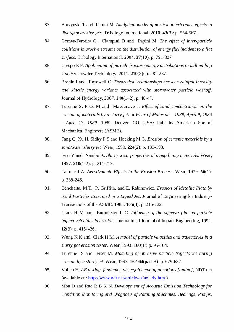
194

83. Burzynski T and Papini M. Analytical model of particle interference effects in

divergent erosive jets. Tribology International, 2010. 43(3): p. 554-567.

84. Gomes-Ferreira C, Ciampini D and Papini M. The effect of inter-particle

collisions in erosive streams on the distribution of energy flux incident to a flat

surface. Tribology International, 2004. 37(10): p. 791-807.

85. Crespo E F. Application of particle fracture energy distributions to ball milling

kinetics. Powder Technology, 2011. 210(3): p. 281-287.

86. Brodie I and Rosewell C. Theoretical relationships between rainfall intensity

and kinetic energy variants associated with stormwater particle washoff.

Journal of Hydrology, 2007. 340(1–2): p. 40-47.

87. Turenne S, Fiset M and Masounave J. Effect of sand concentration on the

erosion of materials by a slurry jet. in Wear of Materials - 1989, April 9, 1989

- April 13, 1989. 1989. Denver, CO, USA: Publ by American Soc of

Mechanical Engineers (ASME).

88. Fang Q, Xu H, Sidky P S and Hocking M G. Erosion of ceramic materials by a

sand/water slurry jet. Wear, 1999. 224(2): p. 183-193.

89. Iwai Y and Nambu K. Slurry wear properties of pump lining materials. Wear,

1997. 210(1-2): p. 211-219.

90. Laitone J A. Aerodynamic Effects in the Erosion Process. Wear, 1979. 56(1):

p. 239-246.

91. Benchaita, M.T., P. Griffith, and E. Rabinowicz, Erosion of Metallic Plate by

Solid Particles Entrained in a Liquid Jet. Journal of Engineering for Industry-

Transactions of the ASME, 1983. 105(3): p. 215-222.

92. Clark H M and Burmeister L C. Influence of the squeeze film on particle

impact velocities in erosion. International Journal of Impact Engineering, 1992.

12(3): p. 415-426.

93. Wong K K and Clark H M. A model of particle velocities and trajectories in a

slurry pot erosion tester. Wear, 1993. 160(1): p. 95-104.

94. Turenne S and Fiset M. Modeling of abrasive particle trajectories during

erosion by a slurry jet. Wear, 1993. 162-64(part B): p. 679-687.

95. Vallen H. AE testing, fundamentals, equipment, applications [online], NDT.net

(available at : http://www.ndt.net/article/az/ae_idx.htm ).

96. Mba D and Rao R B K N. Development of Acoustic Emission Technology for

Condition Monitoring and Diagnosis of Rotating Machines: Bearings, Pumps,

http://www.ndt.net/article/az/ae_idx.htm

195

Gearboxes, Engines, and Rotating Structures. The Shock and Vibration Digest,

2006. 38(1): p. 3-16.

97. Shehadeh M F. Monotoring of long steel pipes using acoustic emission, PhD

thesis. 2006, Heriot-Watt University: Edinburgh, UK.

98. Schofield B H. Research on the sources and characteristics of acoustic

emission. ASTM STP 505, 1972: p. 11-19.

99. Sikorska J. The application of acoustic emission monotoring to the detection of

flow condition in centrifugal pumps., PhD thesis. 2006, University of Western

Australia, Perth, Australia.

100. Holroyd, T.J., The Acoustic Emission & Ultrasonic Monotoring Handbook.

2000, Oxford.

101. Boschetto A and Quadrini F. Powder size measurement by acoustic emission.

Measurement, 2011. 44(1): p. 290-297.

102. Ivantsiv V, Spelt J K and Papini M. Mass flow rate measurement in abrasive

jets using acoustic emission. Measurement Science & Technology, 2009. 20(9)

doi:10.1088/0957-0233/20/9/095402

103. Faisal N H A, Reuben R L and Alcock B. AE monitoring and analysis of

HVOF themal spraying process. Jornal of Thermal Spray Technology, 2011:

p. 1-14.

104. Mohan R S, Momber A W and Kovacevic R. Detection of Energy Absorption

during Abrasive Water Jet. American Society of Mechanical Engineers,

ASME, 1995. 3(1): p. 69-86.

105. Boness R J and McBride S L, Adhesive and abrasive wear studies using

acoustic emission techniques. Wear, 1991. 149(1-2): p. 41-53.

106. Matsuoka K, Forrest D and Ming-Kai T, On-line wear monitoring using

acoustic emission. Wear, 1993. 162-164(1): p. 605-610.

107. Mechefske C K and Sun G. Monitoring Sliding Wear using Acoustic Emission.

International Congress on Condition Monitoring COMADEM 2001,

Manchester, UK.

108. Nivesrangsan P. Multi-source, multi-sensor approaches to disel engine

monitoring using acoustic emission, PhD thesis 2004, Heriot Watt University:

Edinburgh, UK.

109. Pollock A A. Classical wave theory in practical AE testing. Progress in

Acoustic Emission III – Japanese Society of Non-Destructive Testing, 1986:

p. 708-721.

http://dx.doi.org/10.1088/0957-0233/20/9/095402

196

110. Cochran W, Cooley J, Favin D, Helms H, Kaenel R, Lang W, Maling G,

Nelson D, Rader C and Welch P. What is the fast Fourier transform? IEEE

Transactions on Audio and Electroacoustics, 1967. 15(2): p. 45-55.

111. Welch P. The use of fast Fourier transform for the estimation of power spectra:

A method based on time averaging over short, modified periodograms. IEEE

Transactions on Audio and Electroacoustics, 1967. 15(2): p. 70-73.

112. McFadden P D and Smith J D. Vibration monitoring of rolling element

bearings by the high-frequency resonance technique — a review. Tribology

International, 1984. 17(1): p. 3-10.

113. ASTM standard, E976-99: Standard guide for determining the reproducibility

of acoustic emission sensor response. Annual Book of ASTM Standards, 1999.

3.03: p. 395-403.

114. Brucato A, Grisafi F and Montante G. Particle drag coefficients in turbulent

fluids. Chemical Engineering Science, 1998. 53(18): p. 3295-3314.

115. Heuer V, Walter G and Hutchings I M. A study of the erosive wear of fibrous

ceramic components by solid particle impact. Wear, 1999. 225-229(1):

p. 493-501.

197

Appedix A: AE sensor calibration certificate.

MONITORING PARTICLE IMPACT ENERGY USING ACOUSTIC …

Documents

Transcript of MONITORING PARTICLE IMPACT ENERGY USING ACOUSTIC …