Monitoring and Control of Smart Wells - Stanford University

MONITORING AND CONTROL OF

SMART WELLS

A REPORT SUBMITTED TO THE DEPARTMENT OF

ENERGY RESOURCES ENGINEERING

OF STANFORD UNIVERSITY

IN PARTIAL FULFILLMENT OF THE REQUIREMENTS

FOR THE DEGREE OF MASTER OF SCIENCE

By

Zeid M. Al-Ghareeb

June 2009

iii

©Copyrights by Zeid Alghareeb 2009

All Rights Reserved

v

I certify that I have read this report and that in my opinion

it is fully adequate, in scope and in quality, as partial

fulfillment of the degree of Master of Science in Petroleum

Engineering.

__________________________________

Prof. Roland Horne

(Principal Advisor)

vii

Abstract

Smart wells, wells equipped with smart completion, provide great potential to

improve the recovery from hydrocarbon resources. Smart wells provide the ability to

control uncertainties associated with reservoir heterogeneity. One example is to

mitigate unexpected water production due to fractures and hence increase the

ultimate recovery. This is achieved by selectively controlling production from

multiple laterals. Due to subsurface communication between laterals that have

different productivity indices, it is difficult in practice to optimize production from

smart wells. The optimization of smart wells involves more than one parameter.

These parameters include the settings of the downhole inflow control valves (ICV)

that act as a subsurface chokes.

This research focused on the reservoir engineering aspects of finding the

optimum ICV configuration that optimizes reservoir performance parameters such

as recovery factor and net present value. Also, the work studied the effect of

heterogeneity, mainly fractures, on the optimization process. This research also

proposed a technique to quantify the effect of fractures on the optimization process

to provide recommendations of further analysis.

Genetic algorithm (GA) was used as the main optimization engine to find the

optimum ICV configuration. The GA was accompanied by a data library (proxy) to

reduce the number of required simulation runs. The commercial reservoir simulator

Eclipse was used as the objective function evaluator that assesses how good an

ICV configuration is.

Several examples are presented to show the improvement in reservoir

parameters made using the optimization process. These examples include a

synthetic model, and real onshore and offshore models. Various objective functions

were optimized such as water cut minimization, and net present value

maximization.

ix

Acknowledgment

First and foremost, I would like to express my sincere gratitude and appreciation

to my advisor Prof. Roland Horne. His guidance, inspiration, and insights made

this work possible. His wide knowledge, expert advice, and charming way of

teaching are beyond description and will be of great value to me.

I would like to also thank my colleagues Obi Isebor for helping me with setting

up the genetic algorithm main routine, Jerome Onwunalu for the many useful

suggestions, and my two officemates Alejandro and Mike for the great company

during the many late nights of studying. My special thanks go to the small Saudi

community at Stanford for the priceless gatherings during the two years.

I am indebted to my mentor at Saudi Aramco Mr. Shamsuddin Shenawi for

allowing me to be an additional burden in his busy schedule. Thanks go to my

superiors Mr. Saad Al-Garni, Mr. Methgal Al-Shammari, and Mr. Bevan Yuen for

providing me with all help and logistic support.

I also must thank my parents. They taught me many important lessons in my

life and gave me all their love and support through every stage of my life and my

education. I am very grateful to them. I also need to thank my older brother Fahad

for the invaluable advice and the entertaining conversations from Australia.

Lastly and mostly, all love and appreciation go to my wife Mariam and my son

Mohammed for showering me with all the love and support during the difficult

times. Coming home to see them everyday was all I needed. This work is dedicated

to them.

xi

Table of Contents

Abstract ................................................................................................................... vii

Acknowledgment .................................................................................................... ix

List of Figures ...................................................................................................... xiii

List of Tables .......................................................................................................... xv

1. Introduction ......................................................................................................... 1

1.1. General Background .................................................................................... 1

1.2. Literature Survey ......................................................................................... 4

1.3. Problem Description ..................................................................................... 5

2. Optimization Tools .............................................................................................. 7

2.1. Genetic Algorithm ........................................................................................ 7

2.1.1. Terminology ....................................................................................... 8

2.1.2. Genetic Algorithm Engine .............................................................. 11

2.1.3. GA Solution Representation ........................................................... 11

2.1.3.1. GA Encoding Example ........................................................ 12

2.2. Numerical Reservoir Simulator ................................................................. 15

2.2.1. Multilateral Wells Representation ................................................. 15

2.2.2. ICV Representation......................................................................... 16

2.3. ICV Design ................................................................................................. 19

2.4. Optimization Framework .......................................................................... 20

3. Applications on Various Reservoir Models ................................................. 23

3.1. Synthetic Model – Water Cut Minimization ............................................. 23

3.1.1. The Synthetic Model ....................................................................... 23

3.1.2. Optimum ICV Setting – Water Cut Minimization ........................ 27

xii

3.2. Offshore Model – Net Present Value Maximization ................................. 29

3.2.1. The Offshore Model ......................................................................... 29

3.2.2. Optimum ICV Setting – NPV Maximization ................................. 33

3.3. Onshore Model – Production Plateau ....................................................... 38

3.3.1. The Onshore Model ......................................................................... 38

3.3.2. Optimum ICV Setting – Production Plateau ................................. 42

4. Fractures Effects on Smart Wells Optimization ......................................... 47

4.1. Fracture Representation ............................................................................ 50

4.2. Fracture Location Study ............................................................................ 52

4.3. Fracture Location Study Framework ........................................................ 53

4.4. Onshore Model Fracture Study – Case One ............................................. 54

4.4.1. Onshore Model – Case 1a ............................................................... 56

4.4.2. Onshore Model – Case 1b ............................................................... 56

4.5. Onshore Model Fracture Study – Case Two ............................................. 57

4.5.1. Onshore Model - Case 2a ................................................................ 58

4.5.2. Onshore Model – Case 2b ............................................................... 59

5. Conclusions and Future Work ........................................................................ 61

5.1. Conclusions ................................................................................................. 61

5.2. Future Work ............................................................................................... 62

Nomenclature ......................................................................................................... 63

Bibliography ........................................................................................................... 65

Appendix A .............................................................................................................. 67

Appendix B .............................................................................................................. 70

xiii

List of Figures

Figure 1-1: Schematic of components of a multilateral smart well (Dumville, 2008)

..................................................................................................................................... 2

Figure 1-2: Production target achieved by a lower number of smart wells

(Mubarak et al., 2007) ................................................................................................. 2

Figure 2-1: Decimal and binary individuals .............................................................. 8

Figure 2-2: Presentation of generations within GA ................................................... 8

Figure 2-3: Transition from one generation to the next .......................................... 10

Figure 2-4: Crossover operator ................................................................................. 10

Figure 2-5: Mutation operator .................................................................................. 10

Figure 2-6: Binary form of solution .......................................................................... 12

Figure 2-7: Fitness value for continuous and binary encodings ............................. 14

Figure 2-8: Average fitness value vs. generation .................................................... 14

Figure 2-9: Structure of keyword WSEG with two laterals emanating from the

motherbore ................................................................................................................ 16

Figure 2-10: Eclipse ICV file ................................................................................. 18

Figure 2-11: Flowchart of the optimization framework .......................................... 22

Figure 3-1: Synthetic model permeability distribution and producer location ...... 25

Figure 3-2: Oil flow rate vs. ICV setting when only one lateral is producing ........ 26

Figure 3-3: oil flow rate vs. ICV setting when all laterals are producing .............. 27

Figure 3-4: Solution surface with lateral two kept at fully open position .............. 28

Figure 3-5: Progress of GA optimization for the Synthetic model .......................... 29

Figure 3-6: Offshore model 3D grid structure and initial water saturation .......... 30

Figure 3-7: Offshore model - permeability distribution of layer nine ..................... 32

Figure 3-8: Offshore model - production rate and water cut (base case) ................ 33

Figure 3-9: Offshore model - individual lateral production rate (base case) .......... 34

Figure 3-10: Offshore model - individual lateral water cut (base case) .................. 34

Figure 3-11: Solution surface with lateral-0 (MB) fully closed ............................... 35

xiv

Figure 3-12: Progress of GA optimization for the offshore model ........................... 36

Figure 3-13: Offshore model - production rate and water cut (optimized case) ..... 37

Figure 3-14: Offshore model - individual lateral production rate (optimized case) 37

Figure 3-15: Onshore model 3D grid structure and initial water saturation ......... 39

Figure 3-16: Onshore model – five-spot pattern on saturation map ....................... 41

Figure 3-17: Onshore model – production rate and water cut (base case) ............. 44

Figure 3-18: Onshore model - individual lateral production rate (base case) ........ 44

Figure 3-19: Onshore model – production rate and water cut (optimized case) ..... 45

Figure 3-20: Onshore model - individual lateral production rate (optimized case) 45

Figure 4-1: Fractures and matrix in reservoir (Warren and Root, 1963) ............... 47

Figure 4-2: Fracture imaging log showing fracture spacing, formation orientation,

and dip ....................................................................................................................... 49

Figure 4-3: Source model technique as discrete fracture (Voelker, 2004) .............. 50

Figure 4-4: Source model representation as a curved fracture (Voelker, 2004) ..... 51

Figure 4-5: Multiple realizations comprising an area of possible fracture location

................................................................................................................................... 52

Figure 4-6: Framework of fracture location study ................................................... 53

Figure 4-7: location of study areas in Case 1a and Case 1b .................................... 55

Figure 4-8: Onshore model - permeability and porosity of Case 1a and Case 1b ... 55

Figure 4-9: location of study areas in Case 2a and Case 2b .................................... 57

Figure 4-10: Onshore model - permeability and porosity of case 2a and case 2b ... 58

xv

List of Tables

Table 2-1: MATLAB GA Toolbox options ......................................................... 11

Table 2-2: Summary of problem parameters ................................................... 13

Table 3-1: Synthetic model - reservoir and rock properties ............................ 24

Table 3-2: Synthetic model - fluid properties ................................................... 24

Table 3-3: Areas corresponding to ICV settings for the synthetic models ...... 26

Table 3-4: Offshore model - reservoir and rock properties .............................. 30

Table 3-5: Offshore model – fluid properties ................................................... 31

Table 3-6: Areas corresponding to ICV settings for the offshore models ........ 32

Table 3-7: Onshore model - reservoir and rock properties .............................. 39

Table 3-8: Onshore model – fluid properties .................................................... 40

Table 3-9: Onshore model - production well properties ................................... 41

Table 3-10: Areas corresponding to ICV settings for the onshore model........ 42

Table 4-1: Comparison of fracture location effect – case 1a ............................ 56

Table 4-2: Comparison of fracture location effect – case 1b ............................ 57

Table 4-3: Comparison of fracture location effect – case 2a ............................ 59

Table 4-4: Comparison of fracture location effect – case 2b ............................ 59

1

CHAPTER 1

1. Introduction

1.1. General Background

Well design and planning has advanced during the last two decades, from

conventional vertical wells to nonconventional horizontal wells (NCWs) using

directional drilling technology. Nonconventional wells range from simple horizontal

wells with single wellbore to complex multilaterals even with multiple sublaterals

(fishbone wells).

Nonconventional wells offer more cost-effective alternatives to conventional

wells in terms of drilling, completion, surface equipment, and long-term operation

costs. Production targets are achieved with a far smaller number of nonconventional

wells as they provide better reservoir exposure. From a reservoir management point

of view, nonconventional wells improve productivity index (PI) by maximizing

reservoir contact, minimizing water coning by operating at lower drawdown, and

increasing sweep efficiency by redistributing production along the horizontal

section.

A „smart‟ or „intelligent‟ well is considered one of the most advanced types of

nonconventional wells. A typical smart well is equipped with a special completion

that has packers or sealing elements which allow partitioning of the wellbore,

pressure and temperature sensors and downhole inflow control valves (ICV)

installed on the production tubing, Figure 1-1. The sensors allow continuous

monitoring of pressure and temperature while the ICVs provide the flexibility of

controlling each branch of a multilateral well independently. A smart well can be

either a multilateral well where every lateral is controlled by an ICV or a single

bore well where each segment is controlled by an ICV.

2

Most of the recent oil and gas fields developments in Saudi Arabia are furnished

with smart wells. They provide the desired production target with lower capital and

operating costs. Figure 1-2 shows a comparison between vertical, horizontal, and

smart wells that were deployed in different developments within the same field. 48

smart wells achieved the desired production target as opposed to 150 vertical wells.

(Mubarak, Pham, Shamrani, and Shafiq, 2007)

Figure 1-1: Schematic of components of a multilateral smart well (Dumville, 2008)

Figure 1-2: Production target achieved by a lower number of smart wells (Mubarak et al., 2007)

Packer Control Unit Choke Valve

Lateral#0

Lateral#1

Lateral#2

0

20

40

60

80

100

120

140

160

Plant X Plant Y Plant Z

Num

ber o

f Well

s Re

quire

d

48 Smart Wells

150 Vertical Wells

66 horizontal Wells

3

The advantages of smart wells have been demonstrated in practical applications

for both single and multiple reservoir production (non-commingled production).

Because of their ability to control production from each lateral or segment through

ICV adjustment and manipulation, smart wells can mitigate water production by

allocating the optimum production rate and therefore increase the ultimate

recovery.

Unlike conventional wells where only surface control is used to determine the

optimum production rate, optimization of smart wells requires determining the best

combination of ICV settings (ICV configuration) that yields the highest recovery

factor and hence profit. In the case of commingled production, laterals or branches

are in contact with each other within the immediate vicinity of the reservoir. This

adds another dimension to the optimization process as one lateral might affect the

production of other laterals (in the case of water breakthrough).

Reservoir engineering practices follow two approaches in optimizing oil

production from smart wells. These approaches are the reactive approach and the

proactive approach. The reactive approach is usually achieved on a trial and error

basis, making decisions based on current conditions. A series of production tests is

made to determine the best ICV configuration. A portable multiphase flow meter

(MPFM) is usually used for a faster decision. The reactive approach mainly corrects

for any deviation from the production target; i.e. fast increase in water cut due

to heterogeneity. On the other hand, a proactive approach uses an optimization

algorithm to achieve the best ICV configuration that yields maximum oil recovery

over a period of time in particular making estimates of future events. The proactive

approach also takes advantage of the availability of real time production data which

allows for better decisions. Although the reactive approach is very successful in

correcting deviations from production target as they happen, it may not result in

maximum oil recovery.

4

The main objective of this study was to propose an optimization technique as a

proactive approach to optimize the production from smart wells. The optimization

technique entails the use of genetic algorithm, applied in conjunction with a

commercial reservoir simulator that is capable of modeling ICVs. This study also

assessed the value of knowing fracture locations and their effect on the optimum

ICV settings.

1.2. Literature Survey

Various reactive procedures and proactive techniques have been proposed to

optimize production from smart wells. Mubarak, Pham, Shamrani, and Shafiq

(2007) performed an intensive production test as a reactive measure to eliminate

water production from a trilateral smart well. Although their production test

procedure was determined based on their observations in the field, some interesting

results and observations that could be considered in a proactive approach have been

revealed. Among these observations was the laterals‟ sensitivity to the ICV setting.

In one lateral, a low ICV setting completely eliminated water production as the

water production was a result of water coning through nearby vertical fracture. On

the other hand, a low ICV setting slightly reduced water production in another

lateral and shut-in of that lateral was necessary as the source of water in this case

was the advanced water injection flood front. Jalali, Bussear, and Sharma (1998)

successfully increased the deliverability of a smart gas well drilled in a two-layer

system by producing the top layer without downhole restriction and gradually

unchoking the bottom layer as the bottom hole pressure declined.

Yeten, Durlofsky and Aziz (2002) described a gradient-based technique to

maximize cumulative oil recovery from smart wells. Their optimization technique

was performed over discretized time steps to ensure that earlier ICV settings

determined for earlier time steps would not have negative effects at later time.

Naus, Dolle, and Jansen (2006) proposed a workflow in which a production engineer

can determine the change in flow rate as a result of a change in the ICV setting.

5

The workflow used an algorithm that required instantaneous and derivative

information. The performance of their algorithm was tested in two reservoir cases

with the objective of maximizing ultimate recovery. The optimization resulted in

accelerated production but not necessarily higher ultimate recovery. Brouwer and

Jansen (2002) investigated the impacts of smart completions with different well

targets and constraints; i.e. BHP or liquid rate using optimal control theory. Their

results showed that wells operating with rate control have the ability to accelerate

production and increase ultimate recovery. Alhuthali, Datta-Gupta, Yuen, and

Fontanilla (2009) presented waterflood optimization using smart wells and optimal

rate control. Their approach relied on equalizing the streamline time of flight at the

producing wells to maximize sweep efficiency. Yeten (2003) proposed a general

methodology to optimize the type of nonconventional well, trajectory, location, and

ICV setting. His method was based on genetic algorithm coupled with hill climbing

and artificial neural networks.

1.3. Problem Description

A smart well is best drilled in reservoirs where wellbore hydraulics (water coning or

cusping) and heterogeneity (fractures causing early water breakthrough) exist.

Therefore, eliminating water coning and delaying water breakthrough by

determining the best ICV configuration provides considerable scope for improving

oil and gas production. This study used stochastic methods such as genetic

algorithm to find the optimum ICV configuration. In addition, this study

investigated the effect of heterogeneity, mainly fractures, on the optimization

technique. As mentioned earlier, the laterals or segments of smart wells might be in

contact with each other within the reservoir. This indicates that if one lateral

experiences an early water breakthrough due to fractures existence, the overall

production from the well will be affected.

7

CHAPTER 2

2. Optimization Tools

2.1. Genetic Algorithm

Genetic algorithm (GA) was first described by John Holland in 1975 and developed

by him, his students, and his colleagues. The algorithm is modeled on the principle

of evolution via natural selection (Goldberg, 1989). GA search is based on combining

survival of the fittest with random information exchange. GA is considered a global

optimization method that only uses the objective function value (fitness) as a source

of evaluation instead of using derivative or gradient information to guide the

search. GA searches the solution domain by creating a random set (initial

generation) of binary strings (individuals). GA continues to span the solution

domain by introducing new sets of artificial strings using bits and pieces of the

fittest individuals from previous generations. Unlike other methods, GA uses

probabilistic transition rules to guide the search.

GA was chosen as the optimization tool to find the optimum ICV configuration

because it is:

a global search method that is applicable for functions with local optima;

applicable for discontinuous functions where derivatives can not be obtained;

well-suited for parallel computation which increases the optimization speed;

easy to hybridize with other optimization algorithms.

8

2.1.1. Terminology

Before we discuss how genetic algorithm works, it is essential to introduce some

basic terminology of GA that will be mentioned extensively in this report.

Individual: an individual is a member of a population that contains a potential

solution to the optimization problem. An individual can be represented as a

binary string or a decimal string, Figure 2-1. Both the decimal string and the

binary string shown in Figure 2-1 carry the same information. Assuming that

every three bits in the binary string represent a decimal number, we get

V1 = 5, V2 = 2, V3 = 6.

Figure 2-1: Decimal and binary individuals

Population size: if a population size is three, then three individuals will be

grouped together to form a population.

Generation: is a term that indicates an iteration to be taken within the GA. Each

generation contains a predefined population size, Figure 2-2 . The larger the

number of generations, the higher the probability that the GA will find the

optimum point in the search domain. The cost of optimization increases as the

number of generations increases.

1 0 1 0 1 0 1 1 0

5 2 6Decimal string

Binary string

V1 V2 V3

Generation 1 Generation 2 Generation N

Individual 1

Individual 2

Individual n

Individual 1

Individual 2

Individual n

Individual 1

Individual 2

Individual n

Figure 2-2: Presentation of generations within GA

9

Fitness score: is assigned to each individual according to how good the

solution carried by the individual is. For example, the fitness may be

represented as the oil production if we are trying to maximize oil recovery.

The highly fit individuals (high fitness score) are given more opportunities to

“reproduce”. The least fit individuals on the other hand are less likely to get

selected for reproduction, and therefore die out.

Elitism: is a concept in GA which indicates that the best individual in a population

is replicated into the next population without any alteration. The use of

elitism guarantees that the best individual will not be degraded by the process

of mutation or crossover.

Parents: are a couple of individuals that are selected based on their fitness score

and mated to produce new offspring to replace lower fitness score individuals

in the next generation.

Offspring: are individuals that are created as a result of mating two parents.

Offspring share some features taken from both parents.

Selection: is a sampling process applied to the current generation to create an

intermediate generation. Crossover and mutation are applied to the

intermediate population to create the next population, Figure 2-3.

Crossover: is one of three operators that result in creating new individuals.

Crossover is applied randomly to paired individuals (parents) with a

probability pc to form two new offspring that are inserted into the next

generation, Figure 2-4. Prior to crossover, the population is shuffled by the

selection process.

Mutation: is responsible for flipping a bit in one or more individuals within the

population, when a random drawn value is less than the mutation probability

pm, Figure 2-5. Mutation probability is typically between 0.1% - 1.0%.

Mutation is applied after crossover.

10

Figure 2-3: Transition from one generation to the next

Figure 2-4: Crossover operator

Figure 2-5: Mutation operator

11

2.1.2. Genetic Algorithm Engine

MATLAB® Genetic Algorithm Toolbox, part of MATLAB Optimization Toolbox, was

the main optimization engine used for this problem. The GA Toolbox is closely

integrated with other optimization tools such as pattern search, conjugate gradient,

and steepest descent. GA can be used to find a good starting point to an

optimization problem for instance while pattern search can improve the quality of

the solution. The GA Toolbox features a graphical user interface, the ability to solve

constrained problems, the flexibility to modify and create selection, crossover, and

mutation functions, and the capability for parallelization (“Genetic Algorithm and

Direct Search Toolbox 2”).

Table 2-1: MATLAB GA Toolbox options

Function MATLAB GA Toolbox options

Creation Uniform

Fitness Scaling Rank-based, proportional, linear scaling

Selection Roulette, stochastic uniform, tournament

Crossover Arithmetic, scattered, heuristic, single-point

Mutation Adaptive, feasible, Gaussian, uniform

Plotting Best fitness, best individual, selection index

2.1.3. GA Solution Representation

Before GA can be run, a suitable coding or representation for a potential solution to

an optimization problem must be devised. It is useful to represent the solution as a

set of parameters that are joined together to form a string of values. GA MATLAB

offers two types of solution forms depending on the type of problem:

Binary form

Binary form represents variables in binary space using 0‟s and 1‟s. It is suitable for

discontinuous problems such as ICV configuration problems where an ICV cannot

be open at position 2.316 for example. Binary forms run faster than other forms of

12

coding because the solution can only be represented by integers. Binary forms

require decoding the variables before using them in the objective function. Binary

forms are superior to other forms of encoding when the possible solution boundary

is large.

Real form

Real form is a more intuitive process. It does not require decoding and it is suitable

for problems where the solution is a real number; i.e. production well rate

optimization. Continuous forms require a larger population size to search the bigger

solution space and therefore it takes longer time.

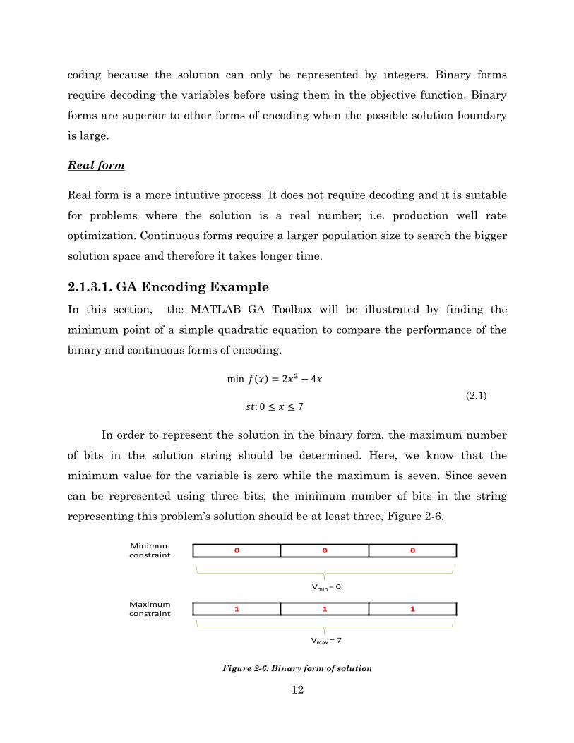
2.1.3.1. GA Encoding Example

In this section, the MATLAB GA Toolbox will be illustrated by finding the

minimum point of a simple quadratic equation to compare the performance of the

binary and continuous forms of encoding.

(2.1)

In order to represent the solution in the binary form, the maximum number

of bits in the solution string should be determined. Here, we know that the

minimum value for the variable is zero while the maximum is seven. Since seven

can be represented using three bits, the minimum number of bits in the string

representing this problem‟s solution should be at least three, Figure 2-6.

Figure 2-6: Binary form of solution

0 0 0Minimum constraint

1 1 1Maximum constraint

Vmin = 0

Vmax = 7

13

On the other hand, the continuous form does not require any sort of encoding and

can be simply represented as any number between the minimum and maximum

constraints.

Table 2-2: Summary of problem parameters

Parameter Option

Population size 9

Generation number 3

Elite count 1

Crossover function Scattered

Crossover fraction 0.8

Mutation function Gaussian

Selection function Stochastic uniform

In order to fairly compare the two forms of encoding, the optimization is repeated

ten times for each form. Figure 2-7 shows the optimization solution (fitness value)

for both forms of encoding. It is worth noting that the success rate of the binary

encoding was 70% while the success rate of the continuous encoding was only 10%.

Seven out of ten trials succeeded in finding the true minimum when using binary

encoding (blue bars in Figure 2-7), whereas only one out of ten succeeded when

using continuous enconding (red bards in Figure 2-7). It is likely that the

continuous encoding may have achieved more successes if has more generations

been computed, although this would have been at greater computational cost.

Figure 2-8 shows the average fitness value for all generations for both forms of

encoding. Although, both the binary and continuous forms are converging toward

the actual minimum fitness value as generations are formed, Figure 2-8 gives a

clear indication that the quality of generations in the binary form is superior

(average fitness value is always closer to the true minimum fitness value).

14

Figure 2-7: Fitness value for continuous and binary encodings

Figure 2-8: Average fitness value vs. generation

-2.5

-2

-1.5

-1

-0.5

0

0.5

1 2 3 4 5 6 7 8 9 10

Fitn

ess

valu

e

Trials

Contineous encoding Vs. Binary encoding

Binary Contieous actual value

2

4

6

8

10

12

14

16

18

20

1 2 3

Ave

rage

Fit

ness

val

ue

Generation

Average fitness value Vs. Generation

Binary Contineous

15

2.2. Numerical Reservoir Simulator

Schlumberger GeoQuest‟s Eclipse was used as the numerical reservoir simulator

in this research. Eclipse can easily implement many types of production and

economic constraints through its existing keywords. These constraints include

economic production limit, production rate limit, and bottom hole pressure limit

(BHP). Eclipse will evaluate the objective function that determines how good an

ICV configuration is. A communication between Eclipse and GA MATLAB was

established so that Eclipse can evaluate the proposed configuration of ICVs and

send the results back to GA MATLAB to proceed further in the optimization

process. However, before we explain how Eclipse communicates with GA

MATLAB, it is crucial to discuss the important keywords used in Eclipse to

represent a multilateral well and ICVs.

2.2.1. Multilateral Wells Representation

Eclipse has the capability to model multilateral wells via the keyword WSEGS.

WSEGS can be used to represent a single well with multiple segments or a

multilateral well with horizontal branches. If a multilateral well is desired, the

point in the motherbore at which a new branch emanates should be defined, Figure

2-9. Although not discussed in this report, special care should be taken when a

branch is not completed at the center of the reservoir grid blocks. Proper well index

values (WI) must be supplied to correct for any branch that is not completed at the

center of the grid blocks.

16

Figure 2-9: Structure of keyword WSEG with two laterals emanating from the motherbore

2.2.2. ICV Representation

Eclipse includes several keywords that can be used to restrict fluid flow. These

keywords include WSEGVALVE, WSEGLABY, and WSEGFILM. All keywords apply the

same restriction mechanism which is imposing additional friction pressure loss

between the sand face and the tubing. The choice of the keyword depends on the

physical means by which the restriction is achieved. For example, WSEGLABY

imposes friction pressure by diverting fluid from the sand face to flow through a

helical path of small channels. The friction pressure in this case is a function of the

diameter of the flow channels and the length of the device. Although this keyword

can achieve flow restriction, it is physically impossible to adjust the length of the

device or the diameter of the flow channel periodically.

In this problem, WSEGVALVE keyword is chosen to represent ICVs. It represents a

subcritical valve that imposes an additional pressure drop due to flow through a

constriction with a specified area of cross section. The pressure drop across an ICV

Seg. Start # Seg. End # Branch # Seg. Join # X Y

2 2 1 1 11 1

3 3 1 2 11 2

4 4 1 3 11 3

5 5 1 4 11 4

6 6 1 5 11 5

7 7 1 6 11 6

8 8 1 7 11 7

9 9 1 8 11 8

10 10 1 9 11 9

11 11 1 10 11 10

12 12 1 11 11 11

13 13 1 12 11 12

14 14 2 6 11 6

15 15 2 14 12 6

16 16 2 15 13 6

17 17 2 16 14 6

18 18 2 17 15 6

19 19 2 18 16 6

20 20 2 19 17 6

21 21 2 20 18 6

22 22 3 5 11 5

23 23 3 22 10 5

24 24 3 23 9 5

25 25 3 24 8 5

26 26 3 25 7 5

27 27 3 26 6 5

28 28 3 27 5 5

29 29 3 28 4 5

30 30 3 29 3 5

31 31 3 30 2 5

0

2

4

6

8

10

12

14

0 2 4 6 8 10 12 14 16 18 20

Lateral 0 Lateral 1 Lateral 2

17

is calculated using a homogeneous model of subcritical flow through a tube

containing a constriction:

(2.2)

where:

accounts for pressure drop due to flow through constriction and is

calculated by:

(2.3)

where:

is a unit conversion constant

is the density of the fluid mixture

is the volumetric rate of the fluid mixture

is the cross-section area of the constriction

is a dimensionless flow coefficient for the valve

accounts for any additional pressure drop due to flow in the horizontal

lateral. It is calculated using the standard expression for the

homogeneous flow frictional pressure loss through a pipe:

(2.4)

where:

is the Fanning friction factor

is the length of the tube in the horizontal lateral

is the diameter of the pipe

is the area of the tube

18

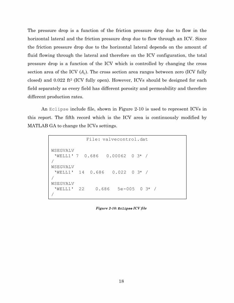
The pressure drop is a function of the friction pressure drop due to flow in the

horizontal lateral and the friction pressure drop due to flow through an ICV. Since

the friction pressure drop due to the horizontal lateral depends on the amount of

fluid flowing through the lateral and therefore on the ICV configuration, the total

pressure drop is a function of the ICV which is controlled by changing the cross

section area of the ICV ( ). The cross section area ranges between zero (ICV fully

closed) and 0.022 ft2 (ICV fully open). However, ICVs should be designed for each

field separately as every field has different porosity and permeability and therefore

different production rates.

An Eclipse include file, shown in Figure 2-10 is used to represent ICVs in

this report. The fifth record which is the ICV area is continuously modified by

MATLAB GA to change the ICVs settings.

Figure 2-10: Eclipse ICV file

File: valvecontrol.dat

WSEGVALV

‘WELL1' 7 0.686 0.00062 0 3* /

/

WSEGVALV

‘WELL1' 14 0.686 0.022 0 3* /

/

WSEGVALV

‘WELL1' 22 0.686 5e-005 0 3* /

/

19

2.3. ICV Design

Several production simulations should be carried out to design and optimize the

ICV sizing. Production rates vary from one field to another and are function of the

ICV size. In order to find the optimum ICV configuration that optimizes an objective

function whether it is maximizing oil recovery, maximizing net present value or

minimizing water production ICVs should be designed in such a way that each

setting yields different production rate and therefore significantly impact the

optimization process.

The ICV design process depends mostly on the production capability of each

lateral. However, most oil companies generalize the design process and make it

depend on the average field production rate rather than individual laterals

production rates. The constant field design is better for logistic purposes such as

maintenance and surveillance work. Since all the cases that will be shown in the

subsequent chapters include only one well in each example field, ICV design will

depend on the production rate from each individual lateral.

According to Equation 2.2, the total pressure drop ( ) is the sum of pressure

drop due to fluid flow through the ICV ( and the horizontal section ( .

Pressure drop due to the ICV depends mostly on the area open to flow and the

magnitude of the production rate ( . Pressure drop in the horizontal section also

depends on the production rate and Fanning friction factor ( which indirectly

depends on production rate through the Reynolds number. The variable production

rate and the fact that the produced fluid is multiphase (multiphase flow creates

different fluid regimes) result in different Fanning friction factor and therefore

variable total pressure drop. The variable total pressure drop term indicates a

nonlinear relationship between the ICV setting and the production rate.

For the purpose of this research, ICV size was chosen to best fit each

optimization problem. ICV settings were discretized so each setting gave more or

20

less equal production rate even though sometimes that is impossible. Below are

some considerations that have been made when designing the ICV:

Simulation runs were performed to determine the maximum and minimum

production rates for each lateral for two cases. These cases were when all

laterals were producing together and when only one lateral was producing at

a time.

The area of an ICV was discretized based on the minimum and maximum

production rate. The number of intermediate ICV settings is usually

predefined by the manufacturing company.

The minimum ICV setting corresponded to zero production rate while the

maximum ICV setting corresponded to the maximum production rate.

If production rate was significantly different from one lateral to another,

ICVs with different sizes were applied although this might not be a feasible

approach for all oil companies.

The new ICV settings were tried out on the two cases; the case with all

laterals producing, Figure 3-3, and the case with only one lateral producing

at a time, Figure 3-2. If more than half of the ICV settings in a lateral gave

the same production rate, this was taken to show that the maximum

production rate should be reduced.

2.4. Optimization Framework

A flowchart of the overall optimization process is shown in Figure 2-11. The figure

shows how MATLAB GA communicates with Eclipse to send and receive

optimization parameters.

In step one, a population of binary strings is created. An individual is

converted to the corresponding decimal string in step two. Then the decimal string

is discretized to the desired number of ICVs settings. For example, a nine-bit binary

string is converted to three-part decimal string which corresponds to three ICVs

21

settings. Since 99% of the optimization CPU time is spent in evaluating the

objective function (i.e. the reservoir simulations), a library is created for each

reservoir realization. The library contains any ICV setting that was proposed by the

MATLAB GA and its corresponding objective function result (i.e. NPV). Before the

ICVs settings are sent to the simulator, the optimization code checks the library for

any identical ICVs settings ran earlier. If these settings are available, the simulator

will not run and the CPU time will be saved. If the ICVs settings are not available,

they will be written in a text file to be supplied to Eclipse. In step six, Eclipse is

run with the supplied ICVs settings. Once the simulation run is finished, the

MATLAB GA reads the simulated parameters, i.e. cumulative oil production and

cumulative water production in this problem, and calculates the objective function.

These steps are repeated for each individual in the population before the selection

process takes place. At this time, the ICV setting and its corresponding objective

function value will be stored in the library for future use. Once all individuals are

simulated, the GA ranks these individuals based on their fitness function ratio and

then selects the individuals that will contribute to the creation of the next

generation. GA operators such as crossover, mutation, and elitism are applied to the

selected individuals to form the next generation. The whole process is repeated for

the next generations until termination criteria are met. The GA will be terminated

if the specified generation number is reached or if there is no improvement in the

objective function for 50 consecutive generations.

22

Create a population of binary strings

Convert a binary string to a decimal string

Transform the decimal string into corresponding ICV areas

Does ICV configuration exist

in the library?

NO

Write ICV configuration in Eclipse file

Run Eclipse

Read output

Calculate objective function

Is population size = # strings simulated?

YES

NO

YES

Select and rank individuals

Apply GA operators: crossover, mutation, elitism

Stop criteria met?Return best individual that

yields highest objective function

NO YES

Ne

w o

ffsp

rin

g c

rea

ted

Store ICV configuration and the corresponding objective function value

Figure 2-11: Flowchart of the optimization framework

23

CHAPTER 3

3. Applications on Various Reservoir Models

This chapter will present the applications of the optimization methodology to three

different reservoir models. The complexity of the reservoir models increased from a

simple synthetic model to dual porosity, highly fractured model. Thus, high impact

GA parameters such as population size and generation number were chosen on a

case-by-case basis to ensure optimum results are attained. In addition, ICVs sizes

were determined for each case to ensure that each ICV setting can provide different

production rate. Different objective functions such as recovery factor, net present

value and water cut minimization were evaluated. The optimum ICV setting were

determined using exhaustive search for all three cases to compare the true global

solution to that obtained using the optimization method. This provided the

opportunity to evaluate the effectiveness of the optimization methodology and the

impact of various GA parameters.

3.1. Synthetic Model – Water Cut Minimization

3.1.1. The Synthetic Model

The synthetic model is a heterogeneous, isotropic, two dimensional, fluvial channel

reservoir model. The reservoir dimensions are 2000×2000×50 ft3 on a 40×40×1 grid.

Permeability values range from 0.45 md to 52 md and the distribution is given in

Figure 3-1. Porosity was taken to be constant with a value of 0.3. Reservoir, rock,

and fluid properties are given in Table 3-1 and Table 3-2. The reservoir is producing

under five-spot pattern where a producer is placed at the middle of the reservoir

(20×20) and four injectors are placed at the corners. The producer is a trilateral

smart well where each lateral intersects 400 ft of the reservoir while the injectors

are conventional vertical wells. Water is injected at a target rate of 300 STB/D in

24

each injection well with a maximum bottomhole pressure of 8000 psi. Production is

specified to occur at a target oil rate of 300 STB/D with a minimum bottom hole

pressure of 100 psi. A minimum oil production rate of 100 STB/D was imposed as an

economic constraint. The simulation was run for 1200 days.

Table 3-1: Synthetic model - reservoir and rock properties

Reservoir and rock properties

Reservoir size 2000×2000×50 ft3

Oil thickness 50 ft

Porosity 0.3

kx = ky = kz 100 md

Compressibility 0.5×10-5psi-1 @ 14.7 psi

krw 0.029 @ Sw = 0.2

kro 0.0838 @ Sw = 0.2

Pbub 3824 psi

OWC 9000 ft

Table 3-2: Synthetic model - fluid properties

Density (lbm/ft3) Viscosity (cp)

Oil 54 1.16@ 14.7 psi

Water 58 1 @ 14.7 psi

25

Bottomhole pressure control strategy usually results in a large change in oil

production during the first couple of years. For instance, oil production rate dropped

by 40% in the first three years in this case. Since ICV settings were predetermined

to be eight to match most ICVs used in the oil industry, the maximum ICV size was

chosen based on the average oil production rate during the first three years rather

than the maximum oil production rate, while the minimum ICV size was chosen to

give zero oil production rate, Table 3-3. This ensures that each setting will produce

more or less equal change in oil production.

5 10 15 20 25 30 35 40

5

10

15

20

25

30

35

40

5

10

15

20

25

30

35

40

45

50

L1

L3

L2

Figure 3-1: Synthetic model permeability distribution and producer location

26

Table 3-3: Areas corresponding to ICV settings for the synthetic models

Setting Area (ft3)

0 0

1 0.000038

2 0.00008

3 0.00013

4 0.00019

5 0.00027

6 0.00038

7 0.00057

On the other hand, individual lateral oil production rate is different when

each lateral produces by itself from that when they all produce together. This

difference is significant in the case of lateral two and therefore settings six and

seven did not change the production rate, Figure 3-3.

Figure 3-2: Oil flow rate vs. ICV setting when only one lateral is producing

0

500

1000

1500

2000

2500

0 1 2 3 4 5 6 7

Oil

flow

rate

(STB

/D)

ICV setting

MB L-1 L-2

27

Figure 3-3: oil flow rate vs. ICV setting when all laterals are producing

3.1.2. Optimum ICV Setting – Water Cut Minimization

The objective was to find the optimum ICV configuration that yields the minimum

water cut. Production and injection controls have been specified so that all possible

ICV configurations are capable of producing 300 STB/D of oil for 1200 days. This

will ensure fair and consistent comparison. Exhaustive search has been made to

determine the global optimum ICV configuration. Knowing the global optimum ICV

configuration provided the opportunity to evaluate the effectiveness of the

optimization by comparing to the results of the exhaustive search. Also, the fact

that water cut was determined at every possible ICV configuration allowed for

intensive sensitivity analysis without the need to perform additional simulations.

Since all configurations are capable of achieving the production target, the

optimized parameter (which is water cut) is affected by heterogeneity; i.e.,

permeability, and its influence on water front advancement. It was realized from

the exhaustive search that the optimum ICV configuration is (0,7,0) meaning that

both laterals one and three are closed while lateral two is fully open. In fact, any

0

200

400

600

800

1000

1200

1400

1600

1800

0 1 2 3 4 5 6 7

Oil

flow

rate

(STB

/D)

ICV setting

MB L-1 L-2

28

ICV configuration that involves laterals one and three being closed will yield the

minimum water cut. Figure 3-4 shows the effect of laterals one and three on the

optimum solution, with lateral two being kept fully open. We can see how water cut

increases as we open both laterals one and three.

Figure 3-4: Solution surface with lateral two kept at fully open position

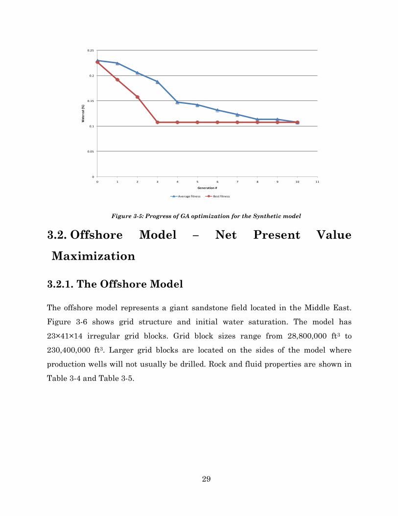
Analysis was carried out to test the GA optimization performance. As

mentioned earlier, a population size of nine (which is equivalent to the solution

string length) was used for ten generations. Figure 3-5 shows the progress of the

optimization run in terms of the average value of the fitness function, water cut in

this case, and the best individual. It is worth noting that the average water cut

decreased drastically in the early stages until it became equal to the best individual

at the end of the optimization run. In addition, the value of the best individual

reached the global optimum solution which is at WC = 10.81% on the third

generation. This is a clear indication that GA optimization is suitable for the

problems of this type due to the fast rate of convergence.

29

Figure 3-5: Progress of GA optimization for the Synthetic model

3.2. Offshore Model – Net Present Value

Maximization

3.2.1. The Offshore Model

The offshore model represents a giant sandstone field located in the Middle East.

Figure 3-6 shows grid structure and initial water saturation. The model has

23×41×14 irregular grid blocks. Grid block sizes range from 28,800,000 ft3 to

230,400,000 ft3. Larger grid blocks are located on the sides of the model where

production wells will not usually be drilled. Rock and fluid properties are shown in

Table 3-4 and Table 3-5.

0

0.05

0.1

0.15

0.2

0.25

0 1 2 3 4 5 6 7 8 9 10 11

Wat

er cu

t (%

)

Generation #

Average fitness Best fitness

30

Figure 3-6: Offshore model 3D grid structure and initial water saturation

Table 3-4: Offshore model - reservoir and rock properties


model size 23×41×14 grid blocks

Oil thickness 136 ft

Porosity 0.23

Average permeability 300 md

kv/kh ratio 0.05

Compressibility 6.8×10-6psi-1 @ 300 psi

krw 0.05 @ Sw = 0.57

kro 0.04 @ Sw = 0.57

krg 0.054 @ Sg = 0.53

Original reservoir pressure 2316 psi @ 4370 ft SS

Pbub 876 psi

OWC 5052 ft SS

31

Table 3-5: Offshore model – fluid properties

Density (lbm/ft3) Viscosity (cp) FVF (V/V)

Gas 46.80 0.0205 @ 3000 psi 0.8790 @ 3000 psi

Oil 55.36 2.58 @ 3000 psi 1.4361 @ 3000 psi

Water 72.38 1 @ 3000 psi 1.003 @ 3000 psi

The field is currently undeveloped. So, a smart well is placed as a proof of

concept to test and evaluate the technology on reservoir, well performance, and

overall reservoir management strategies. The reservoir is producing under primary

recovery and the production well is placed downdip to ensure water production

toward the end of the simulation run. The production well is a trilateral smart well

where each lateral intersects approximately 10,000 ft of the ninth layer of the

reservoir. Figure 3-7 shows the permeability map of layer nine. Production is

specified to occur at a target oil rate of 4,000 STB/D with a minimum bottom hole

pressure of 1000 psi. A minimum oil production rate of 100 STB/D was imposed as

an economic constraint. In addition, a maximum water production of 400 STB/D

was imposed. The simulation was run for 10 years.

Production control strategy was used in the simulator specification to ensure

a constant oil rate of 4,000 STB/D is produced. Although individual laterals might

not produce the target rate, ICVs were designed to ensure a combined target rate of

4,000 STB/D. ICV settings and the corresponding areas are given in Table 3-6.

32

Figure 3-7: Offshore model - permeability distribution of layer nine

Table 3-6: Areas corresponding to ICV settings for the offshore models

Setting Area (ft3)

0 0

1 0.00006

2 0.00021

3 0.00026

4 0.00041

5 0.00065

6 0.0011

7 0.0080

33

3.2.2. Optimum ICV Setting – NPV Maximization

The objective in this case was to find the optimum ICV configuration that yields the

maximum net present value (NPV). The production well was specified to produce at

a controlled rate of 4,000 STB/D even though some ICV configurations might not be

able to. In addition, the production well was allowed a maximum water production

of 400 STB/D. This increased the weight of water production in the objective

function and avoided the trivial optimum fully open ICV configuration (7,7,7). NPV

was calculated with a net oil profit of $50/bbl and water handling cost of $20/bbl.

This case was first simulated with the trivial ICV configuration of (7,7,7)

which comprises the base case. Figure 3-8 shows the production well rate and the

corresponding water cut. The production rate was initially 1600 STB/D and the

decline was very shallow. The shallow decline in production rate indicates that the

production well is capable of producing the target rate of 4,000 STB/D. However, the

production well is restricted to maintain the target water production limit of 400

STB/D. Figure 3-10 shows that lateral-0 (MB) was the main source for water

production. So, intuitively restricting lateral-0 will boost the cumulative production

up although lateral-0 produces high oil rate.

Figure 3-8: Offshore model - production rate and water cut (base case)

0

0.05

0.1

0.15

0.2

0.25

0.3

0.35

0.4

0

500

1000

1500

2000

2500

3000

3500

4000

4500

1 2 3 4 5 6 7 8 9 10 11

Wat

er cu

t (%)

Oil r

ate (

STB/

D)

Time (years)

Oil rate WC

34

Figure 3-9: Offshore model - individual lateral production rate (base case)

Figure 3-10: Offshore model - individual lateral water cut (base case)

Exhaustive search indicateed that the optimum ICV configuration is (0,4,7).

Although it was a high producing lateral, lateral-0 was fully closed to minimize

water production and release the overall restriction on the well. It has been seen

previously that lateral-0 was the main source of water. Lateral-2 was fully open

because lateral-2 is already a low producing lateral with no water production. So, it

0

500

1000

1500

2000

2500

1 2 3 4 5 6 7 8 9 10 11

Oil r

ate (

STB/

D)

Time (years)

Lateral-0 (MB) Lateral-1 Lateral-2

0

0.05

0.1

0.15

0.2

0.25

0.3

1 2 3 4 5 6 7 8 9 10 11

Wat

er cu

t (%

)

Time (years)


35

makes a perfect sense to produce as much as possible from lateral-2 since it does not

add any water production. With lateral-0 closed, lateral-1 has to be open to a certain

degree to compensate the loss in oil production. We can see that lateral-1 is

adjusted at setting four which balances oil production and water production. Figure

3-11 shows the effect of lateral-1 and lateral-2 on NPV. NPV drops when ICV2 is

greater than four.

Figure 3-11: Solution surface with lateral-0 (MB) fully closed

Analysis was carried out to test the GA optimization performance. Similar to

the synthetic case, a population size of nine was used for twenty generations. Figure

3-12 shows the progress of the optimization run in terms of the average value of the

fitness function, NPV in this case, and the best individual. The average NPV is

noted to increase rapidly during the first five generations. In addition, the value of

the best individual reacheed the global optimum solution which is at NPV = 654.5

MM$ on the fifth generation. This indicates that a population size that is equivalent

to the solution string length and a generation number of five was adequate for this

case.

36

Figure 3-12: Progress of GA optimization for the offshore model

Figure 3-13 and Figure 3-14 show the cumulative and individual lateral oil

production rates. We can see in the optimized case that the production well is now

able to maintain the target rate of 4,000 STB/D throughout the simulation run time

with minimum water production. In addition, lateral-0 (MB) which was the main

source of water is closed completely. The loss in oil production was compensated by

moderately producing from lateral-1.

0

100

200

300

400

500

600

700

800

0 5 10 15 20 25

NPV

(MM

$)

Generation #

Average fitness Best fitness

37

Figure 3-13: Offshore model - production rate and water cut (optimized case)

Figure 3-14: Offshore model - individual lateral production rate (optimized case)

0

0.05

0.1

0.15

0.2

0.25

0.3

0.35

0.4

0

500

1000

1500

2000

2500

3000

3500

4000

4500

1 2 3 4 5 6 7 8 9 10 11

Wat

er cu

t (%)

Oil r

ate (

STB/

D)

Time (years)

Oil rate WC

0

500

1000

1500

2000

2500

1 2 3 4 5 6 7 8 9 10 11

Oil

rate

(STB

/D)

Time (years)


38

3.3. Onshore Model – Production Plateau

3.3.1. The Onshore Model

The onshore model represents a sector model of an onshore field located in the

Middle East. The field is a giant anticline trap that produces from two main

reservoirs. These reservoirs are an upper and lower carbonate reservoirs separated

by a thick non-reservoir formation. The upper reservoir is prolific throughout the

entire field with an average vertical permeability of 400 md while the lower

reservoir has an average vertical permeability of 1-2 md only. Although these

reservoirs are separated by a thick non-reservoir layer, production data suggests

that vertical communication between the two reservoirs exists and is believed to be

caused by fractures that cut through the non-permeable layer. The onshore model

contains square grid blocks. It focuses only on the top reservoir which

is divided into 26 layers. Figure 3-15 shows the grid structure and initial water

saturation. Rock and fluid properties are available in Table 3-7 and

39

Table 3-8. The simulation was run for 20 years.

Figure 3-15: Onshore model 3D grid structure and initial water saturation

Table 3-7: Onshore model - reservoir and rock properties


model size 12,750×4,750×6,500 m3

Porosity 0.16

kx 546 mD

ky 401 mD

kz 11.6 mD

Compressibility 2.0×10-6 psi-1 @ 3410 psi

krw 0.32 @ Sw = 0.54

kro 0.005 @ Sw = 0.54

krg 0.067 @ Sg = 0.54

Initial reservoir pressure 3524.9 psi

Initial water saturation 0.712

Pbub 2533.5 psi

40

Table 3-8: Onshore model – fluid properties

Density (lbm/ft3) Viscosity (cp) FVF (V/V)

Gas 0.06095 @ 14.7 psi 0.0112 @ 14.7 psi 0.84 @ 3330 psi

Oil 52.36 @ 14.7 psi 1.34 @ 14.7 psi 1.0764 @ 14.7 psi

Water 71.85 @ 14.7 psi 1 @ 14.7 psi 1.0207 @ 3400 psi

The field is very mature and producing under secondary recovery. The

production well was drilled as a trilateral smart well in the west side of the model

sector (I = 15, J = 12) in the first layer. Laterals two and three are close to vertical

fractures network suggested by loss of circulation while drilling. The production

well properties are given in Table 3-9. Production was specified to occur at a target

oil rate of 3,000 STB/D with a minimum bottom hole pressure of 1800 psi. A

minimum oil production rate of 100 STB/D was imposed as an economic constraint.

A five-spot injection scheme that consists of four power water injection wells (PWI)

injected water at a constant rate of 20,000 STB/D (5000 STB/D/Well) in layers 3

through 26 allowing bottom-up sweep behavior. These four wells are located at the

corners of the sector, Figure 3-16 . ICVs were designed to handle the target

production rate of 3,000 STB/D. The ICV settings and the corresponding areas are

given in

41

Table 3-10.

Table 3-9: Onshore model - production well properties

Lateral # No. of segments Length Avg. effective kh

Lateral-0 (MB) 5 6,179‟ 12,453

Lateral-1 6 4,086‟ 12,221

Lateral-2 8 4,333‟ 12,256

Figure 3-16: Onshore model – five-spot pattern on saturation map

I1 I2

I4I3

P1

42

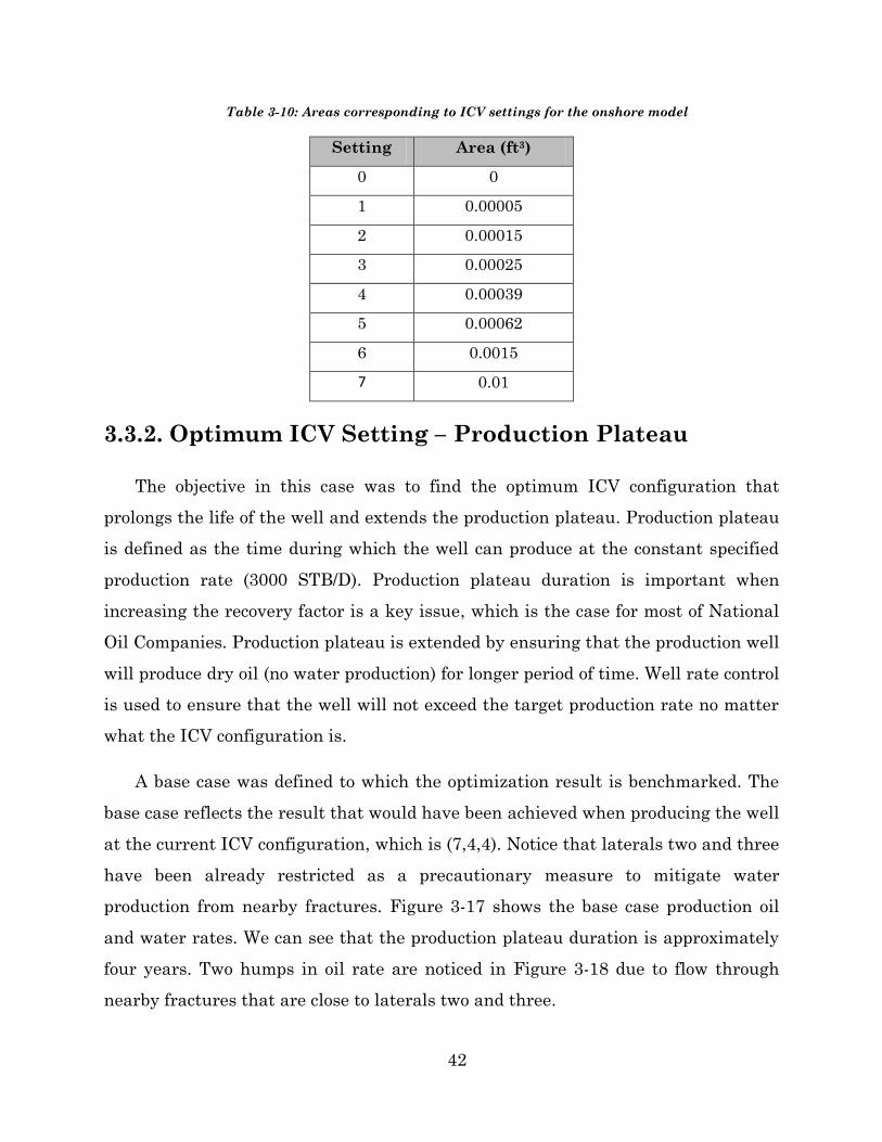
Table 3-10: Areas corresponding to ICV settings for the onshore model

Setting Area (ft3)

0 0

1 0.00005

2 0.00015

3 0.00025

4 0.00039

5 0.00062

6 0.0015

7 0.01

3.3.2. Optimum ICV Setting – Production Plateau

The objective in this case was to find the optimum ICV configuration that

prolongs the life of the well and extends the production plateau. Production plateau

is defined as the time during which the well can produce at the constant specified

production rate (3000 STB/D). Production plateau duration is important when

increasing the recovery factor is a key issue, which is the case for most of National

Oil Companies. Production plateau is extended by ensuring that the production well

will produce dry oil (no water production) for longer period of time. Well rate control

is used to ensure that the well will not exceed the target production rate no matter

what the ICV configuration is.

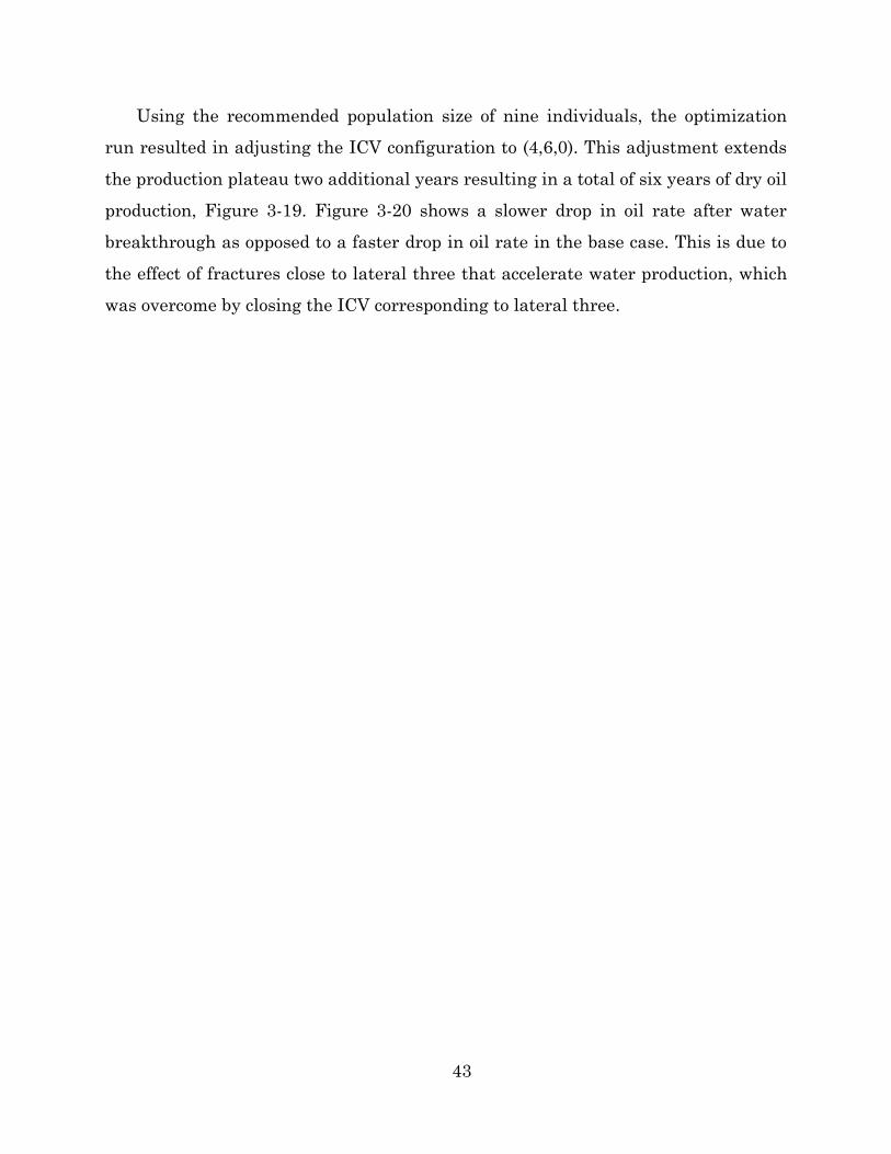
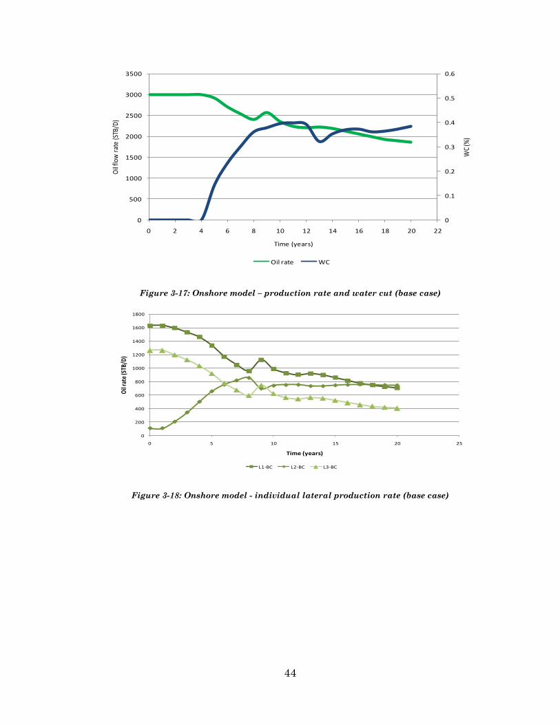
A base case was defined to which the optimization result is benchmarked. The

base case reflects the result that would have been achieved when producing the well

at the current ICV configuration, which is (7,4,4). Notice that laterals two and three

have been already restricted as a precautionary measure to mitigate water

production from nearby fractures. Figure 3-17 shows the base case production oil

and water rates. We can see that the production plateau duration is approximately

four years. Two humps in oil rate are noticed in Figure 3-18 due to flow through

nearby fractures that are close to laterals two and three.

43

Using the recommended population size of nine individuals, the optimization

run resulted in adjusting the ICV configuration to (4,6,0). This adjustment extends

the production plateau two additional years resulting in a total of six years of dry oil

production, Figure 3-19. Figure 3-20 shows a slower drop in oil rate after water

breakthrough as opposed to a faster drop in oil rate in the base case. This is due to

the effect of fractures close to lateral three that accelerate water production, which

was overcome by closing the ICV corresponding to lateral three.

44

Figure 3-17: Onshore model – production rate and water cut (base case)

Figure 3-18: Onshore model - individual lateral production rate (base case)

0

0.1

0.2

0.3

0.4

0.5

0.6

0

500

1000

1500

2000

2500

3000

3500

0 2 4 6 8 10 12 14 16 18 20 22

WC

(%)

Oil

flow

rat

e (S

TB/D

)

Time (years)

Oil rate WC

0

200

400

600

800

1000

1200

1400

1600

1800

0 5 10 15 20 25

Oil

rate

(STB

/D)

Time (years)

L1-BC L2-BC L3-BC

45

Figure 3-19: Onshore model – production rate and water cut (optimized case)

Figure 3-20: Onshore model - individual lateral production rate (optimized case)

0.00

0.10

0.20

0.30

0.40

0.50

0.60

0

500

1000

1500

2000

2500

3000

3500

0 2 4 6 8 10 12 14 16 18 20 22

WC

(%)

Oil

flow

rat

e (S

TB/D

)

Time (years)

Oil rate WC

0

500

1000

1500

2000

2500

3000

0 5 10 15 20 25

Oil

rate

(STB

/D)

Time (years)

L1-OC L2-OC L3-OC

47

CHAPTER 4

4. Fractures Effects on Smart Wells

Optimization

A great portion of the world‟s hydrocarbon exists in naturally fractured reservoirs

(Aguilera, 1995). One example is the largest oil field in the world, the Ghawar field,

which poses a great challenge in terms of fracture complexity. Fractures display

complicated flow behavior due to the extreme difference in permeability and

porosity between the rock matrix and the fracture itself. Fractures have much

greater permeability than the formation they penetrate. A fracture acts as a conduit

or a „highway‟ in the rock that transmits oil and gas which affects the flow behavior

of the porous medium. However, fractures are associated with very low fluid

storativity compared to the rock matrix (Horne 1995, p.36-41). This means that

fractures do not store as much oil and gas as the matrix they reside in.

Figure 4-1: Fractures and matrix in reservoir (Warren and Root, 1963)

48

Fractures can be favorable or unfavorable in terms of hydrocarbon production

(Mavco et al., 1998). For example, hydraulically induced fractures are introduced in

tight gas reservoirs to enhance the low permeability matrix. On the other hand,

fractures may cause water flooding projects to fail due to injected water being

transmitted from injection wells to production wells through fractures leaving large

amounts of bypassed hydrocarbon. This causes premature abandonment of

production wells because of the inability to mitigate the high water production. A

perfect example is the onshore model case discussed in Chapter 3. It has been seen

how restricting production from lateral three which is close to the fracture allowed

the production well to maintain its target and resulted in prolonging the well‟s life.

Fractures can be identified directly using cores, formation imaging logs, and

drill cuttings. Figure 4-2 illustrates a formation imaging log that shows fracture

spacing, formation orientation, and dip. Fractures can also be identified indirectly

by loss of circulation while drilling, very high production in thin zones on production

logs, and using well test analysis. Direct sources of fracture identification require

the fracture to actually intersect the wellbore. Due to the huge difference in size

between the wellbore and the reservoir, the percentage of fractures identified using

direct sources is very small. Indirect sources of fracture identification on the other

hand do not require the wellbore to intersect the fracture. In fact, indirect sources

do not specify the location of the fracture as they only indicate the effect, i.e. earlier

water breakthrough, loss of circulation, and high producing thin zone.

Since the chance that a well will intersect a fracture is slim, the exact

location of a fracture is usually unknown. However, this can be compensated by

approximating the location of the fracture in the reservoir model based on indirect

sources of information at first and performing a series of simulation runs to history

match the effect or anomalies caused by the fracture, i.e., water cut. Although

history matching yields acceptable results, it is computationally expensive as it

requires a large number of parameters to be adjusted. So, this chapter will discuss a

49

technique to investigate whether it is essential to know the exact location of the

fracture to properly optimize the production from a smart well.

Figure 4-2: Fracture imaging log showing fracture spacing, formation orientation, and dip

50

4.1. Fracture Representation

Several techniques have been introduced in the literature to model fractured

reservoirs. One technique used to model fractures is called Discrete Fracture

Network (DFN). DFN is usually used when matrix has very low porosity and

permeability. However, it can be extended to handle high porosity and permeability

reservoirs where the concept of an effective matrix is introduced. In this research, a

fairly new and simple technique called source model will be used as a DFN flow

model. The technique was developed by Voelker in 2004. Source model is simply a

shut-in „well‟ that is not produced at the surface. However, the well is open to

backflow between the source connections (grid blocks intersecting the source)

instead, Figure 4-3. Technically, source model is represented as a group of

connection transmissibilities constrained by a zero flow rate and hydrostatic

equilibrium:

(4.1)

Figure 4-3: Source model technique as discrete fracture (Voelker, 2004)

51

In this research, the transmissibilities of connections are similar to the

transmissibilities of the grid block hosting them since the fractures in this study are

artificial and did not require history matching. Source model can be implemented in

all conventional flow simulators. Advantages of using source model include:

simplicity of implementation: adding DFNs is similar to adding wells and

therefore can be used in multiple realizations.

no alteration of flow simulator grid blocks.

ability to use in mixed fracture system (small scale and large scale fractures).

capability to use sources along a curve, Figure 4-4.

Figure 4-4: Source model representation as a curved fracture (Voelker, 2004)

52

4.2. Fracture Location Study

In order to investigate the sensitivity of the location of fractures on the optimization

of a smart well, multiple realizations have been made. The fracture location in each

realization was different. For a fair comparison between the case where we knew

the fracture location and the case we did not, fractures were placed in the form of a

rectangle that surrounded the actual location of a fracture, Figure 4-5. Although the

exact location of a fracture might have not been known, it could be approximated

using indirect sources.

Figure 4-5: Multiple realizations comprising an area of possible fracture location

The expected value of the objective function of the multiple realizations was used

for evaluation of fitness during the optimization.

(4.2)

where is the case name, and is the realization number.

The expected value of the objective function was compared against the value of the

objective function of the realization with the exact location.

53

4.3. Fracture Location Study Framework

A flowchart of the fracture location study is given in Figure 4-6. In short, each

candidate ICV configuration proposed by the GA was simulated on all reservoir

realizations. The expected value of the objective function was calculated using the

objective function values of all realizations. The expected value was used for

evaluation and progress from one generation to the next. A library, similar to the

one discussed in Chapter 2, was created for each case to minimize the time required

to complete the run.

Figure 4-6: Framework of fracture location study

1 0 1 0 1 0 1 1 0

Verify results with evaluation function

Return bestStop criteriaYN

54

4.4. Onshore Model Fracture Study – Case One

As previously mentioned in Section 3.3.1, the onshore model represents a sector

model of a giant field located in the Middle East. The main producing reservoir

undergoes peripheral waterflood where water injection wells are placed on the

flanks of the field. Since the sector model is approximately at the middle of the field,

the waterflood is compensated by fluxes of oil and water coming from the four sides

of the sector model. The reservoir is heterogeneous, isotropic, and naturally

fractured. Although the reservoir sweep tendency in general is a bottom-up sweep,

DFNs significantly affect specific well performance as water breaks through earlier

in thin intervals. In fact, this phenomenon necessitates the use of Smart completion

and production equalizers as production wells tend to die prematurely due to high

water cut.

The source model approach was used to introduce DFN in two cases. These

cases are Case 1a and Case 1b. Fractures were placed around the actual fracture

comprising a square of 750 m × 750 m, Figure 4-7. The expected NPV which was the

comparison criterion was an average of the NPVs resulted from all fracture

realizations. Since fractures closer to the well normally result in lower NPV while

fractures far away result in higher NPV, the expected NPV is more or less

equivalent for any fracture at similar distance, as is the case for the fracture

realizations shown in Figure 4-7. The permeability and porosity Case 1a and 1b are

shown in Figure 4-8. Production was specified to occur at a target oil rate of 3,000

STB/D in both cases with a minimum bottom hole pressure of 1800 psi.

55

Figure 4-7: location of study areas in Case 1a and Case 1b

Figure 4-8: Onshore model - permeability and porosity of Case 1a and Case 1b

× : anticipated fracture location in a realization+ : actual fracture location

Case 1a Case 1b

Case 1a Case 1b

kx

ky

kz

ф

56

4.4.1. Onshore Model – Case 1a

GA was run for three generations with a total population size of nine to

maximize the objective function, which is NPV in this case. The expected NPV was

compared to its respective base case as in Table 4-1. The base case corresponded to

the case where the location of the fracture was known. This table indicates that the

optimization was not affected by the location of the fracture as long as the fracture

remained within the highlighted area in Figure 4-7. The reason for this is that

water production that affected the motherbore and lateral-3 (indicated by the ICV

restriction) was due mostly to the advancement of the waterflood front. Although

the fractures accelerated water production, water production was overwhelmed by

the waterflood front advancement. The difference in the optimum ICV

configuration in Case 1a and its corresponding base cases was small (within GA

error). It is worth noting that the ICVs were set at a higher position to increase

NPV as the horizontal permeability was relatively lower. The difference in NPV was

also very small which confirms the insensitivity of this case to the location of the

fracture.

Table 4-1: Comparison of fracture location effect – case 1a

NPV Optimum ICV Difference

Base case 1a $622,958,763 (4 5 1) 0.0%

Case 1a $612,538,543 (4 5 0) 1.7%

4.4.2. Onshore Model – Case 1b

Similar to Case 1a, GA was run for three generations with a total of nine

individuals in each population to maximize the NPV which is the comparison basis.

Although Case 1b shows better horizontal permeability and porosity in general

which might increase the effect of fractures in transmitting water to the production

well, it was found out that this case is also insensitive to the fracture location as

long as the fracture is within the highlighted area in Figure 4-7. The water

57

production in this case was coming due to waterflood front from the west and

fractures from the east. However, the fractures did not seem to alter the optimum

ICV configuration even though the expected NPV was lowered by 1.4%. In fact the

difference in NPV between Case 1b and its corresponding base case is only 1.4%,

Table 4-2.

Table 4-2: Comparison of fracture location effect – case 1b


Base case 1b $603,487,630 (4 7 1) 0.0%

Case 1b $595,235,488 (5 7 1) 1.4%

4.5. Onshore Model Fracture Study – Case Two

This case is very similar to Case one. However, the source model DFNs were

arranged to occupy bigger areas as shown in Figure 4-9 for Case 2a and Case 2b. In

addition, the base cases were simulated twice with the actual fracture in different

locations within the candidate fracture area. The permeability and porosity of both

cases are given in Figure 4-10.

Figure 4-9: location of study areas in Case 2a and Case 2b

Case 2a Case 2b

× : anticipated fracture location in a realization+ : actual fracture location

58

Figure 4-10: Onshore model - permeability and porosity of case 2a and case 2b

4.5.1. Onshore Model - Case 2a

The expected NPV which comprised the average value for fracture locations around

the boundary of the candidate area was compared against the NPVs resulted from

the fracture located at grid blocks (12,10) and (13,10). Table 4-3 summarizes the

difference between Case 2a and the base cases. It can bee seen that the difference in

NPV was very small as most of the water production was due to waterflood front

advancement.

Case 2a Case 2b

kx

ky

kz

ф

59

Table 4-3: Comparison of fracture location effect – case 2a


Base case (12,10) $627,788,988 (4 5 0) 0.0%

Base case (13,10) $622,958,763 (4 5 1) 0.8%

Case 2a $623,435,899 (4 5 0) 0.7%

4.5.2. Onshore Model – Case 2b

Now we look at Case 2b where the area of study is located east of the well as in

Figure 4-9. Comparing the NPV from Case 2b and the base case where the fracture

is located at grid block (18,10), we can see a minor difference of 0.97% in NPV. In

addition, the ICV of lateral-1 which in this case sees water production from both

sides did not change. However, the difference in NPV between Case 2b and the base

case where the fracture is in grid block (19,10) rose to 4.9%. This difference altered

the optimum ICV configuration as evident from Table 4-4. The optimum ICV

changed to (6 7 1) as the fracture was placed further away from lateral-1 and

therefore water production brought by the fracture was minimized.

Table 4-4: Comparison of fracture location effect – case 2b


Base case (18,10) $603,487,630 (4 7 1) 0.0%

Base case (19,10) $632,945,410 ( 6 7 1) 4.9%

Case 2b $609,367,689 (4 5 0) 0.97%

Knowing the exact location of the fracture was not essential in Cases 1a and

2a. The reason for this is that water production was mostly caused by the

advancement of the waterflood front. The fractures slightly accelerated water

production. In Cases 2a and 2b, the fractures were far away from the waterflood

front. Although water production was caused by the advancement of floodfront and

the fracture in Case 1b, the optimum ICV configuration remained unchanged due to

the small candidate area. The difference in NPV between Case 1b and its

60

corresponding base case was only 1.4%. However, the difference between Case 2b

and its corresponding base case was 4.9%. This difference altered the optimum ICV

configuration from (4 5 0) to (6 7 1) as the fracture was placed further away from

the production well and therefore water production brought by the fracture was

minimized. Hence, knowing the exact location of the fracture in Case 2b was very

important to the optimization process.

61

CHAPTER 5

5. Conclusions and Future Work

5.1. Conclusions

A general methodology was used to optimize production from smart wells. The

methodology entailed the use of genetic algorithm applied in conjunction with a

commercial reservoir simulator that is capable of simulating ICVs. The methodology

utilized a built-in data library to reduce the number of required runs to find the

optimum ICV configuration.

The general algorithm was applied to several field cases with different

objectives. ICVs were designed for each case to ensure that each setting yielded

different production rates and therefore significantly impacted the optimization

process. Different objectives were achieved using the algorithm. These objectives

include minimizing water cut, extending production plateau, and maximizing NPV.

Applying the algorithm in one case resulted in an extended production plateau of

six years as opposed to four years when using the current ICV configuration.

The leveraged knowledge gained from working these different cases has

provided an insight into the effect of heterogeneity on the optimization

methodology. A technique was proposed to quantify the effect of fractures on the

optimization process. Various reservoir realizations were created to study and

quantify the impact of fractures on the production optimization process. One case

concluded that knowing the fracture location did not affect the optimum ICV

configuration when it was generally close to the injected water floodfront. However,

the fracture location altered the optimum ICV configuration when it was on the

opposite side from the water floodfront.

62

5.2. Future Work

The following items are proposed to improve the optimization of smart wells

production:

Additional search algorithms can be hybridized with GA to increase the

efficiency and speed of the optimization method.

The optimization methodology can be modified to handle the change of ICV

configuration with time.

Rea-time data such as pressure and temperature can be used as evaluation

parameters to provide continuous production optimization. Smart

completions are often equipped with this kind of real-time sensors.

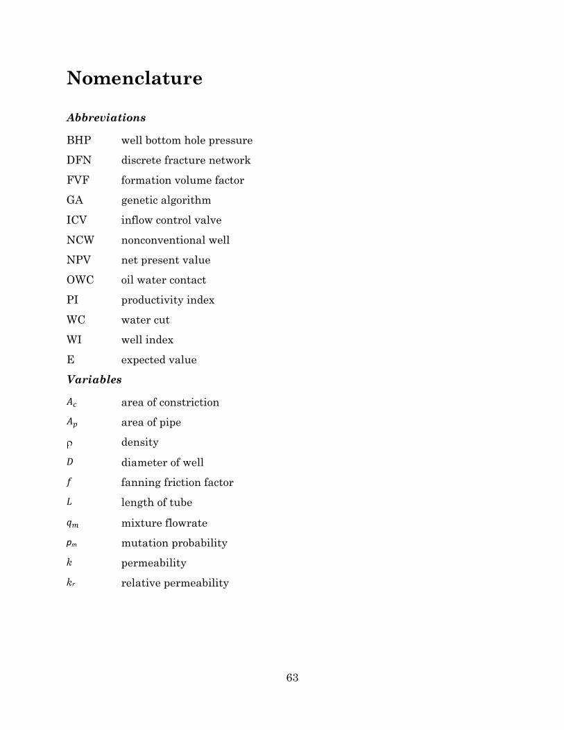
63

Nomenclature

Abbreviations

BHP well bottom hole pressure

DFN discrete fracture network

FVF formation volume factor

GA genetic algorithm

ICV inflow control valve

NCW nonconventional well

NPV net present value

OWC oil water contact

PI productivity index

WC water cut

WI well index

E expected value

Variables

area of constriction

area of pipe

density

diameter of well

fanning friction factor

length of tube

mixture flowrate

pm mutation probability

k permeability

kr relative permeability

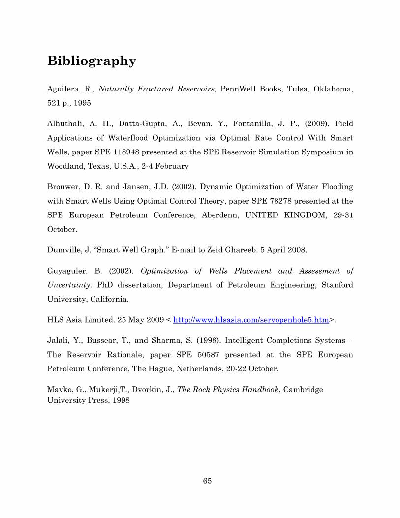
65

Bibliography

Aguilera, R., Naturally Fractured Reservoirs, PennWell Books, Tulsa, Oklahoma,

521 p., 1995

Alhuthali, A. H., Datta-Gupta, A., Bevan, Y., Fontanilla, J. P., (2009). Field

Applications of Waterflood Optimization via Optimal Rate Control With Smart

Wells, paper SPE 118948 presented at the SPE Reservoir Simulation Symposium in

Woodland, Texas, U.S.A., 2-4 February

Brouwer, D. R. and Jansen, J.D. (2002). Dynamic Optimization of Water Flooding

with Smart Wells Using Optimal Control Theory, paper SPE 78278 presented at the

SPE European Petroleum Conference, Aberdenn, UNITED KINGDOM, 29-31

October.

Dumville, J. “Smart Well Graph.” E-mail to Zeid Ghareeb. 5 April 2008.

Guyaguler, B. (2002). Optimization of Wells Placement and Assessment of

Uncertainty. PhD dissertation, Department of Petroleum Engineering, Stanford

University, California.

HLS Asia Limited. 25 May 2009 < http://www.hlsasia.com/servopenhole5.htm>.

Jalali, Y., Bussear, T., and Sharma, S. (1998). Intelligent Completions Systems –

The Reservoir Rationale, paper SPE 50587 presented at the SPE European

Petroleum Conference, The Hague, Netherlands, 20-22 October.

Mavko, G., Mukerji,T., Dvorkin, J., The Rock Physics Handbook, Cambridge

University Press, 1998

http://www.hlsasia.com/servopenhole5.htm

66

Mubarak, S. M., Pham, T. R., Shamrani, S. S., and Shafiq, M. (2007). Using Down-

Hole Control Valves to Sustain Oil Production From the First Maximum Reservoir

Contact, Multilateral and Smart Well in Ghawar Field: Case Study, paper IPTC

11630 presented at the International Petroleum Technology Conference in Dubai,

U.A.E., 4-6 December.

Voelker, J. (2004). A Reservoir Characterization of Arab-D Super-K as A Discrete

Fracture Network Flow System, Ghawar Field, Saudi Arabia. PhD dissertation,

Department of Petroleum Engineering, Stanford University, California.

Warren, J. E., Root, P. J., (1963). The Behavior of Naturally Fractured Reservoirs.

SPE Journal, 3 March.

Yeten, B. (2003). Optimum Deployment of Nonconventional Wells. PhD dissertation,

Department of Petroleum Engineering, Stanford University, California.

Yeten, B., Durlofsky, L. J., Aziz, K., (2002). Optimization of Smart Well Control,

paper SPE/PS-CIM/CHOA 79031 presented at the SPE International Thermal

Operations and Heavy Oil Symposium and International Well Technology

Conference in Calgary, Alberta, CANADA, 4-7 November

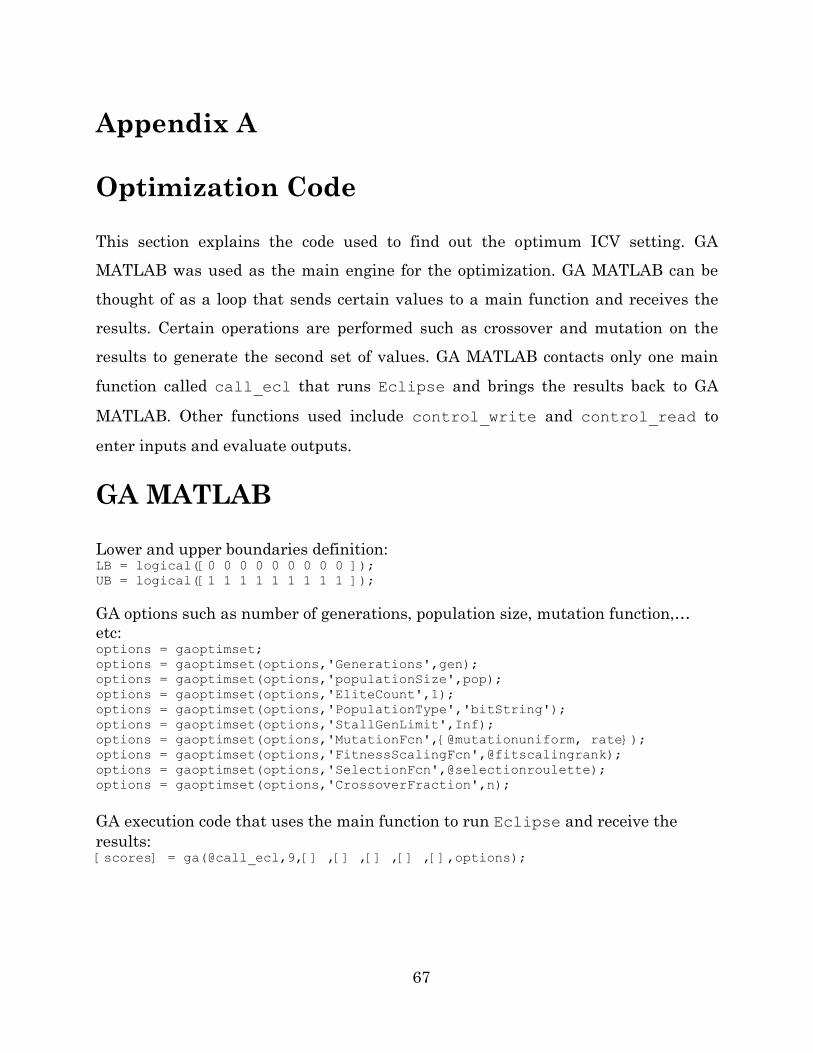
67

Appendix A

Optimization Code

This section explains the code used to find out the optimum ICV setting. GA

MATLAB was used as the main engine for the optimization. GA MATLAB can be

thought of as a loop that sends certain values to a main function and receives the

results. Certain operations are performed such as crossover and mutation on the

results to generate the second set of values. GA MATLAB contacts only one main

function called call_ecl that runs Eclipse and brings the results back to GA

MATLAB. Other functions used include control_write and control_read to

enter inputs and evaluate outputs.

GA MATLAB

Lower and upper boundaries definition: LB = logical([0 0 0 0 0 0 0 0 0 ]); UB = logical([1 1 1 1 1 1 1 1 1 ]);

GA options such as number of generations, population size, mutation function,…

etc: options = gaoptimset; options = gaoptimset(options,'Generations',gen); options = gaoptimset(options,'populationSize',pop); options = gaoptimset(options,'EliteCount',1); options = gaoptimset(options,'PopulationType','bitString'); options = gaoptimset(options,'StallGenLimit',Inf); options = gaoptimset(options,'MutationFcn',{@mutationuniform, rate}); options = gaoptimset(options,'FitnessScalingFcn',@fitscalingrank); options = gaoptimset(options,'SelectionFcn',@selectionroulette); options = gaoptimset(options,'CrossoverFraction',n);

GA execution code that uses the main function to run Eclipse and receive the

results: [scores] = ga(@call_ecl,9,[] ,[] ,[] ,[] ,[],options);

68

Main Routine

The main routine is responsible for supplying ICVs to Eclipse, reading results,

and sending them to GA MATLAB.

Sending the ICVs given by GA MATLAB to the simulator control_write('valvecontrol.dat',x)

Running Eclipse dos('$Eclipse ECL_RUN1 > ecloutput.dat');

Reading the results [WC]=control_read('ECL_RUN1.RSM', columns_number1);

Closing Eclipse dos('del ECL_RUN1.RSM');

Writing Function

This function is responsible for converting ICV settings to the corresponding areas,

and then writing them in the simulator file.

Converting the ICV settings to the corresponding areas if x(1) == 0 y1 = 1e-12; elseif x(1) == 1 y1 = 0.000038; elseif x(1) == 2 y1 = 0.00008; elseif x(1) == 3 y1 = 0.00013; elseif x(1) == 4 y1 = 0.00019; elseif x(1) == 5 y1 = 0.00027; elseif x(1) == 6 y1 = 0.00038; elseif x(1) == 7 y1 = 0.00057; end

Similar work is done for ICV2 and ICV3.

69

Writing the areas in the simulator file

fid = fopen(fle,'w');

fprintf(fid,'WSEGVALV \n'); fprintf(fid,' ''PRODZ'' 2 0.686 %g/ \n',y1); fprintf(fid,'/ \n');



Reading function

fid = fopen(fle,'r');

This loop is used to discard comment lines in the simulator output file for i = 1:10 tline = fgetl(fid); end

Reading the data and converting them to a matrix m = fscanf(fid,'%f'); % reads data from choke.RSM and format as text n1 =reshape(m,columns_number1,length(m)/columns_number1); n1 = transpose(n1);

fclose(fid);

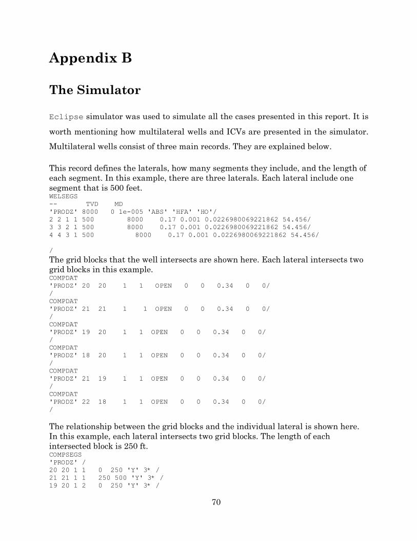
70

Appendix B

The Simulator

Eclipse simulator was used to simulate all the cases presented in this report. It is

worth mentioning how multilateral wells and ICVs are presented in the simulator.

Multilateral wells consist of three main records. They are explained below.

This record defines the laterals, how many segments they include, and the length of

each segment. In this example, there are three laterals. Each lateral include one

segment that is 500 feet. WELSEGS

-- TVD MD

'PRODZ' 8000 0 1e-005 'ABS' 'HFA' 'HO'/

2 2 1 1 500 8000 0.17 0.001 0.0226980069221862 54.456/

3 3 2 1 500 8000 0.17 0.001 0.0226980069221862 54.456/

4 4 3 1 500 8000 0.17 0.001 0.0226980069221862 54.456/

/

The grid blocks that the well intersects are shown here. Each lateral intersects two

grid blocks in this example. COMPDAT

'PRODZ' 20 20 1 1 OPEN 0 0 0.34 0 0/

/

COMPDAT

'PRODZ' 21 21 1 1 OPEN 0 0 0.34 0 0/

/

COMPDAT

'PRODZ' 19 20 1 1 OPEN 0 0 0.34 0 0/

/

COMPDAT

'PRODZ' 18 20 1 1 OPEN 0 0 0.34 0 0/

/

COMPDAT

'PRODZ' 21 19 1 1 OPEN 0 0 0.34 0 0/

/

COMPDAT

'PRODZ' 22 18 1 1 OPEN 0 0 0.34 0 0/

/

The relationship between the grid blocks and the individual lateral is shown here.

In this example, each lateral intersects two grid blocks. The length of each

intersected block is 250 ft. COMPSEGS

'PRODZ' /

20 20 1 1 0 250 'Y' 3* /

21 21 1 1 250 500 'Y' 3* /

19 20 1 2 0 250 'Y' 3* /

71

18 20 1 2 250 500 'Y' 3* /

21 19 1 3 0 250 'Y' 3* /

22 18 1 3 250 500 'Y' 3* /

/

This record defines the ICVs for this well. INCLUDE

'valvecontrol.dat' /

The well‟s target is defined. WCONPROD

PRODZ OPEN ORATE 300 1* 1* 1* 1* 0 /

/

The economic limit of the well is defined. WECON

'PRODZ' 100 1* 0.98 1* 1* 'NONE' 'NO'/

/

Monitoring and Control of Smart Wells - Stanford University

Documents

Transcript of Monitoring and Control of Smart Wells - Stanford University