Monica Billio, Massimiliano Caporin, Loriana Pelizzon and

Domenico Sartore

CDS Industrial Sector Indices,

credit and liquidity risk ISSN: 1827-3580 No. 09/WP/2012

W o r k i n g P a p e r s

D e p a r t me n t o f E c o n o m i c s

C a ’ Fo s c a r i U n i v e r s i t y o f V e n i c e

N o . 0 9 / W P / 2 0 1 2

ISSN 1827-3580

The Working Paper Series

is available only on line

(www.dse.unive.it/pubblicazioni)

For editorial correspondence, please contact:

wp.dse@unive.it

Department of Economics

Ca’ Foscari University of Venice

Cannaregio 873, Fondamenta San Giobbe

30121 Venice Italy

Fax: ++39 041 2349210

CDS Industrial Sector Indices, credit and liquidity risk

Monica Billio Università Ca’ Foscari Venezia

Massimiliano Caporin Università di Padova

Loriana Pelizzon Università Ca’ Foscari Venezia

Domenico Sartore Università Ca’ Foscari Venezia

Abstract

This paper studies the risk spillover among US Industrial Sectors and focuses on the connection between credit and liquidity risks. The proposed methodology is based on quantile regressions and considers the movements of CDS Industrial Sector Indices depending on common risk factors such as equity risk, risk appetite, term spread and TED spread. We use CDS Industrial indexes and the market risk factor to identify the impact of market liquidity risk and market credit risk in the different US Industries and give evidence of the heterogeneity of this relation. We show that all the sectors are largely exposed to the non investment grade bond spread indicating that credit risk is largely a common factor rather than a sector specific factor. With a lower impact, we also find that market risk and interest rate risk are also common factors, as well as liquidity risk. These results indicate that diversification among sectors might collapse when credit, equity and liquidity events hit the market. The information extracted from CDS market could thus provide relevant information for sector allocation strategies.

Keywords

Credit Risk, Common factors, liquidity risk

JEL Codes

F34, G12, G15.

Address for correspondence: Monica Billio

Department of Economics

Ca’ Foscari University of Venice

Cannaregio 873, Fondamenta S.Giobbe 30121 Venezia - Italy

Phone: (++39) 041 2349170

Fax: (++39) 041 2349176 e-mail: billio@unive.it

This Working Paper is published under the auspices of the Department of Economics of the Ca’ Foscari University of Venice.

Opinions expressed herein are those of the authors and not those of the Department. The Working Paper series is designed to

divulge preliminary or incomplete work, circulated to favour discussion and comments. Citation of this paper should consider its

provisional character.

1 Introduction

Is sector credit risk primarily an industry-specific type of risk? Or, is sector credit driven

primarily by common factors? How stable is this relationship? Understanding the nature of

credit risk industrial sectors is of key importance given the large and rapidly increasing size of

the corporate bond and CDS markets. Furthermore, the nature of credit risk industrial sector

directly affects the ability of financial market participants to diversify the risk of debt portfolios.

However, despite the importance of CDS in the financial markets, relatively little research

about the sources of commonality of these financial products has appeared in the literature.

This paper investigates these issues using four different methodologies. We first perform a

simple dynamic correlation analysis. Second, we use principal component analysis to estimate

the number and importance of common factors driving the changes in the CDS indexes. Third,

we consider the Exceedence Correlation (EC) of Longin and Solnik (2001) to investigate the

heterogeneity of the exposures to different observable factors. Fourth, we perform a quantile

regression to investigate the heterogeneity of the exposures among different states of the com-

mon factors. We use an extensive database of Credit Derivatives Swap of US Industrial Sector

Indices.

A Credit Derivatives Swap (CDS) contract is similar to an insurance contract: it obliges

the seller of the CDS to compensate the buyer in the event of loan default. It is a swap because

generally, the agreement is that in the event of default the buyer of the CDS receives money

(usually the face value of the bond), and the seller of the CDS receives the defaulted bond.

This contract therefore is able to measure precisely the credit risk embedded in a corporate

bond.

We consider as observable factors ten different financial variables that are able to capture

common exposure to (i) market risk, (ii) credit risk, (iii) liquidity risk and (iv) interest rate

risk.

Three important results emerge from the analysis. First, the simple correlation analysis

highlights that CDS industrial sector indexes co-move but with different intensity through

time. Second, the co-movements are largely characterized by the common exposure to a single

risk factor, that explain on average 82% of the changes of the 18-CDS indexes. However, this

exposure changes a lot through time (from 33% till 96%) indicating that the relationship is not

stable and not linear. Third, the exposure to credit risk and interest rate risk is non linear, and

is larger when already the high yield bond stread and interest rates faces large cahnges. This

means that there are some amplifying mechanisms in the transmission of credit and interest

2

rate risks. These results indicate that diversification among sectors might collapse when credit

and liquidity events hit the market. The information extracted from CDS market could thus

provide relevant information for sector allocation strategies.

The remainder of the paper is organized as follows. Section 2 describes the data. Section

3 presents the different approaches used to investigate the linearity of the relation across CDS

and its stability and the results. Section 5 concludes.

2 The data

The data for the five-year CDS of US Industrial indexes used in this study are obtained from

Datastream and are based on CDS market quotation data from industry sources. The sample

covers the period from January 2004 untill December 2011.

We have considered the CDS Indexes of 18 sectors: Automobile (AUTOMOB), Banking

(BANKING), Basic Resouces (BASICRES), Chemical (CHEMIC), Construction and materials

(CONSTMAT), Financial services (FINSERV), Food and beverage (FOODBEV), Health care

(HEALTCARE), Industrial goods and Services (INDLGDS), Insurance (INSURAN), Media

(MEDIASEC), Oil and Gas (OILEGAS), Personal and Household Goods (PSNLHSLD), Retails

(RETAILSEC), Technology (TECHNOL), Telecomunication (TELECOM), Travel and Leisure

(TRAVLEI) and Utilities (UTILITIES). The beginning of this sample period is dictated by the

availability of liquid CDS data.

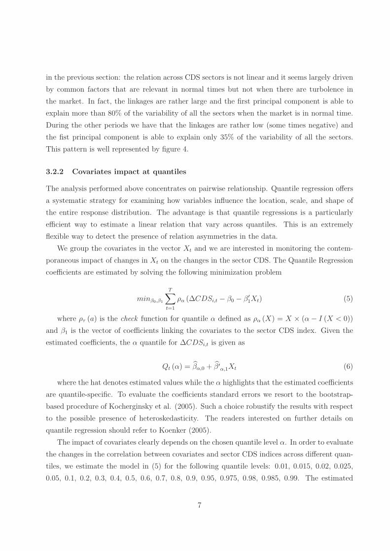
Table 1 provides summary information for the daily CDS Indexes. All CDS Indexes are

denominated in basis points and are, therefore, free of units of account for the CDS swap con-

tracts. The average values of the CDS range widely across indutries. The lowest average is 94.93

basis points for Banking; the highest average is 758 basis points for Automobile sector. Both

the standard deviations and the minimum/maximum values indicate that there are significant

time-series variation in sovereign CDS premiums.

Table 1 also reports the summary statistics of the daily changes in sovereign CDS premiums.

In Figure 1, we report the dynamic of the changes in the CDS spreads through time.

Table 2, to provides additional descriptive statistics, reports the correlation matrix of daily

changes in the five-year CDS Index spreads. Table 2 shows that, while there is clearly signif-

icant cross-sectional correlation in spreads, the correlations are far from perfect. Most of the

correlations are less than 0.7, and a few are negative. The average correlation across the 18

sectors is 0.25.

Since there is virtually an unlimited number of variables that could be related to Industry

3

credit risk, it is important to be selective in the variables considered. We use the daily return

on the NYSE index (log-return) and the daily change in the VIX volatility index from the

financial stock market.

From the bond market, we use the changes in the spreads of U.S. investment-grade and

high-yield corporate bonds. Specifically, we include the change in the spreads between five-year

BBB- and AAA-rated bonds and between five-year BB and BBB-rated bonds. The former

captures the range of variation in investment-grade bond yields, while the latter reflects the

variation in the spreads of high-yield bonds.

From the government bond market, we use ”term spread” calculated as the difference be-

tween the yield to maturity of the 10-year Treasury bond and the 13-week Tbill rate.

Moreover, recent research on corporate credit spreads suggests that these spreads may

include premiums for bearing risks such as jump-to-default risk, recovery risk, the risk of

variation in spreads or distress risk, liquidity risk, etc. As a proxy for the variation in the

equity risk premium, we use monthly changes in the earnings-price ratio for the S&P 100 index.

As another risk premium proxy, we use monthly changes in the spreads between implied and

realized volatility for index options. We use monthly changes in the expected excess returns of

five-year Treasury bonds as a proxy for changes in the term premium.

Liquidity risk is captured using two variables: the change in the difference between the US

repo rate and the 13-week Tbill rate, and the change in the difference between Libor and the

13-week Tbill rate.

Table 3 provides summary statistics of these 10 variables.

Table 4 reports the correlations between the changes in the CDS Indexes and the condi-

tioning variables. As the Table shows, the correlations of the different CDS indexes and the

common factors are quite different; however, the sign of the correlations are almost the same

for all the different sectors.

3 Methodology and Results

3.1 Preliminary analysis

As a first evaluation of the linearity of the relation across CDS and its stability we consider

the rolling evaluation of the linear correlation. We calculate correlation among changes in CDS

spreads considering 60 observations, roughly equivalent to one quarter. The rolling correlation

(average across the 18 sectors correlations) is plotted in Figure 2 from March 2004 through

January 2011. This figure shows overall high values of the correlation between changes in the

4

CDS Indexes (generally between 0.13 and 0.88). Furthermore, we observe that the correlations

across the Industries changes largely through the sample. Starting from December 2008, it has

increased from 0.30 to 0.80. Looking to the last part of the sample it seems that the averall

correlation among the different countries has been reduces. However, this is not the case for

all the Industries. For example, in the last part of the sample the correlation with Utilities and

almost all the other Industries has increases1.

Increased commonality among CDS Sector Indexes can be empirically detected by using

principal components analysis (PCA), a technique in which the changes of the CDS Indexes

are decomposed into orthogonal factors of decreasing explanatory power (see Muirhead, 1982

for an exposition of PCA).

The time-series results for the Cumulative Risk Fraction (i.e., eigenvalues) are presented in

Figure 3. The time-series graph of eigenvalues for the most important principal components

(PC1, PC2, PC3, and PC4) shows that the first principal component captures the majority of

changes in CDS during the whole sample, but the relative importance of these groupings varies

considerably. The time periods when the first principal components explain a larger percentage

of total variation are associated largely with the last part of the sample. In particular, Figure

3 shows that the first principal component is very dynamic, captures from 33% to 99% of CDS

variation, increasing significantly during crisis periods. The PC1 eigenvalue increases from

the beginning of the sample, peaking at 96% in 2004, and subsequently decrease. The PC1

eigenvalue starts to increase in 2005 during the GM/Ford crisis, declines slightly in 2006, and

increases again in 2007 and subsequently decrease. In 2009 it continues to increase in line with

the Sovereign European crisis. As a result, the first principal component explaines 82% of CDS

variation over the 2010-2011. The results show that there is strong commonality in the behavior

of CDS Industrial Indexes.

As a further analysis, we consider the exceedence correlation (EC) of Longin and Solnik

(2001). EC is a conditional correlation measure across two time series. It takes into account

only those observation when the two time series are both above (below) a given empirical

quantile. In formulae, if we consider the quantile or order α, and focus on two economic sectors

i and j, EC is computed as follow:

EC− = Corr [∆CDSi,t,∆CDSj,t|Fi (∆CDSi,t) < q, Fj (∆CDSj,t) < q] , (1)

EC+ = Corr [∆CDSi,t,∆CDSj,t|Fi (∆CDSi,t) > 1− q, Fj (∆CDSj,t) > 1− q] . (2)

where Fi and Fj are the cumulative density functions of the corresponding CDS variations.

1The rolling window correlations among the sector indices are available upon request

5

Therefore, EC is given by two values, EC− measures the correlation in the lower quantiles α,

while EC+ considers observations above 1 − α. EC is generally measured for several values

of α. By convention, the graphs report at the center (for α = 0.5) the full sample standard

correlation, while on the two sides we have EC− (on the left) and EC+ (on the right).

Table 6 presents the summary statistics of the exceedence we have calcualted among the

different sectors. We report the exceedence correlations by reporting in the middle the full

sample standard correlation while on the left and right sides we report ρ− and ρ+, respectively.

As the mean, the min, the maximum and the different percentiles shows, in most cases the

exceedence correlation ρ+ is decreasing as q decreases (note that ρ+ considers the correlation

above the quantile 1− q), suggesting that large positive CDS changes correspond to lower the

correlation across sectors. The same for the opposite: for large negative CDS changes, the

correlation across sectors tends to decrease (in most cases). This result seems to indicate that

the relation the relation across CDS sectors is not linear: is is higher when there are small

positive or negative changes but for large changes in the cds of one sector the relationship is

quite low and in some cases is also negative.

3.2 Common factor analysis

3.2.1 Covariates impact at Exceedence

The relation between the covariates and each economic sector is evaluated using again the

Exceedence measure and the Quantile Regressions.

Regarding the Exceedence measure we have considered the conditional correlation measure

across the CDS Sector ∆CDSi,t and the covariate variable ∆Xj,t.

In formulae, if we consider the quantile or order α, EC is computed as follow:

EC− = Corr [∆CDSi,t,∆Xj,t|Fi (∆CDSi,t) < q, Fj (∆Xj,t) < q] , (3)

EC+ = Corr [∆CDSi,t,∆Xj,t|Fi (∆CDSi,t) > 1− q, Fj (∆Xj,t) > 1− q] . (4)

where Fi and Fj are the cumulative density functions of the corresponding CDS and X

variations.

Table 7 presents the average of the exceedence we have calcualted among the different

sectors. As the Table shows, in most cases the exceedence correlation ρ+ is decreasing as q

decreases, the same for the opposite: for large negative CDS changes, the correlation among

sectors and covariates tends to decrease, suggesting again that large positive or negative CDS

changes correspond to lower the exposures to covariates. This result confirms those obtained

6

in the previous section: the relation across CDS sectors is not linear and it seems largely driven

by common factors that are relevant in normal times but not when there are turbolence in

the market. In fact, the linkages are rather large and the first principal component is able to

explain more than 80% of the variability of all the sectors when the market is in normal time.

During the other periods we have that the linkages are rather low (some times negative) and

the fist principal component is able to explain only 35% of the variability of all the sectors.

This pattern is well represented by figure 4.

3.2.2 Covariates impact at quantiles

The analysis performed above concentrates on pairwise relationship. Quantile regression offers

a systematic strategy for examining how variables influence the location, scale, and shape of

the entire response distribution. The advantage is that quantile regressions is a particularly

efficient way to estimate a linear relation that vary across quantiles. This is an extremely

flexible way to detect the presence of relation asymmetries in the data.

We group the covariates in the vector Xt and we are interested in monitoring the contem-

poraneous impact of changes in Xt on the changes in the sector CDS. The Quantile Regression

coefficients are estimated by solving the following minimization problem

minβ0,β1

T∑

t=1

ρα (∆CDSi,t − β0 − β′1Xt) (5)

where ρτ (a) is the check function for quantile α defined as ρα (X) = X × (α− I (X < 0))

and β1 is the vector of coefficients linking the covariates to the sector CDS index. Given the

estimated coefficients, the α quantile for ∆CDSi,t is given as

Qt (α) = β̂α,0 + β̂′α,1Xt (6)

where the hat denotes estimated values while the α highlights that the estimated coefficients

are quantile-specific. To evaluate the coefficients standard errors we resort to the bootstrap-

based procedure of Kocherginsky et al. (2005). Such a choice robustify the results with respect

to the possible presence of heteroskedasticity. The readers interested on further details on

quantile regression should refer to Koenker (2005).

The impact of covariates clearly depends on the chosen quantile level α. In order to evaluate

the changes in the correlation between covariates and sector CDS indices across different quan-

tiles, we estimate the model in (5) for the following quantile levels: 0.01, 0.015, 0.02, 0.025,

0.05, 0.1, 0.2, 0.3, 0.4, 0.5, 0.6, 0.7, 0.8, 0.9, 0.95, 0.975, 0.98, 0.985, 0.99. The estimated

7

coefficients can be graphically represented together with the corresponding standard errors in

order to evaluate the stability of the relation at different quantiles.

Table 8 reports the estimated coefficients and the t-statistic for all the 18 sectors of the

ten covariates respectively for the 0.05, 0.50 and 0.95 quantiles. Figure 6 shows the number of

significant coefficients for each covariate. Table 8 and Figure 6 show that the covariate that

is highly significant for all the quintiles is the the spreads of high-yield bonds portfolio. This

variable is significant for all the sectors for the 0.95 and 0.50 quantiles and for 17 sectors for

the 0.05 quantiles. This means that the most important common factor is the spread of the

high-yield bonds portofolio, i.e credit risk. Table 8 shows that this factor has the same sign of

impact across quantiles. This result indicates that the credit risk of all the sectors is largely

driven by a common factor that characterizes the probability of default of all the sectors. The

spread of the investment grade portfolio is instead significant for only three sectors and only for

the 0.50 quantile. There is only another factor that is significant for all the different sectors, but

only in the 0.50 percentile: the change in the NYSE. Therefore, the equity market is negatively

affecting the different sector CDSs: an increase in the NYSE reduces the probability of default

of the different firms and therefore the CDS reduces. This second common factor indicates that

when there is a reduction in the equity market the credit risk (and therefore the probability of

default) of all the different sectors is larger.

A factor that is common for 16 out of 18 sectors for the 0.95 quantile and for 15 out of 18

for the 0.50 quantile is the 5 year Treasury Bond rate. The coefficient is positive for all the

sectors. This factor is largely related to the business cycle, i.e. when the Treasury Bond rate

is high, the economy is in a booming state and the probability of default of all the sectors is

lower.

The three variables that are in different ways related to liquidity risk: VIX, TED spread,

Repo-Tbill rate. Among the three the one that is mostly relevant is the TED spread with a

significant impact in different ways when the CDS are increasing and when CDS are decreasing

over lower and hight quantiles. An increase of the TED spread turn to a further increase fo

the CDS low quantile and a reduction on CDS high quantile. This result could be explained

by the fact that when the TED spread is increasing also credit risk is increasing and therefore

the two phenomena should be read together.

The other common factors are significant for a number of sectors that ranges from zero to

11. More specifically, P/E is not relevant, an increase in the risk appetite leads to a lower CDS

change and is significant only for half of the sectors.

The term spread impact in different ways when the CDS are increasing and when CDS are

decreasing over lower quantiles (CDS decreasing): increase in TS turns to a further decrease of

8

CDS (the quantile) over upper quantiles increase in Term Spread provides a further increase of

CDS quantile.

4 Stability of relations

Beside the graphical comparison, some tests might be taken into account to verify the stability

of the covariates impact on the CDS indices.

We take into account two tests. At first, we consider the equality of coefficients across

the highest quantiles and verify the following null hypothesis: H0 : β̂0.90,1 = β̂0.95,1 = β̂0.99,1

and H0 : β̂0.95,1 = β̂0.98,1 = β̂0.985,1 = β̂0.99,1. The test has been proposed by Koenker and

Basset (1982), and is a Wald-type test. Under the null, the test statistic follows a Chi-square

distribution, where the degrees of freedom depend on the number of covariates entering the

equation. When the covariates are K, the degrees of freedom are 2K in the first test, and 3K

in the second case.

Table 9 shows that the null hypothesis of no differences among quantile exposures is rejected

in most of the cases. Therefore, this analysis shows that the exposure to common factors are

largely different when CDS presents positive or negative changes or when changes are large or

small.

We also proceed to verify the stability of coefficients across time. For this purpose we create

a step dummy, Dt which assumes value 1 after date m (and zero before). Then, we estimate

the following quantile regression:

minβ0,β1

T∑

t=1

ρα (∆CDSi,t − β0 − β′1Xt − δ′XtDt) (7)

To null of stability of coefficients in the two subsamples 1 to m and m+1 to T is equivalent

to H0 : δ = 0 and corresponds to a standard test for linear restrictions in the quantile regression

framework (again a Wald-type test).

We have comsidered two subsamples: 2007-2011 and 2009-2011. In all the cases (i.e. 2004-

2001 vs 2007-2011, 2004-2001 vs 2009-2011, 2007-2001 vs 2009-2011) we find that the null

hypothesis of stability of the parameters has been rejected. This confirms the results of the

different appraoaches we have used: the relationship between CDS indexes and common risk

factors are largely unstable through time and heterogeneous among quantiles.

9

5 Conclusions

We study the nature of sectors credit risk using credit default swap data for 18 Industrial

Sectors. We show that credit risk tends to be much more correlated across countries than

are equity index returns for the same countries. Our results suggest that the source of these

higher correlations is the dependence of sector credit spreads on a common set of global market

factors, risk premiums, and liquidity patterns. Specifically, we find that the Sector CDS spreads

are driven primarily by high-yield factors and the Treasury 5 year Bond rate. However, this

relation is not linear and is not stable trough time. Nevertheless, there is strong evidence that

in most of the sample considered common factors are able to explain most of the changes of

CDS Industrial Sector Indices.

References

Duffie, Darrell. 1999. “Credit Swap Valuation.” Financial Analysts Journal, 55(1):

73-87.

Eichengreen, B., and A. Mody (2000), ”What Explains Changing Spreads on Emerging-Market

Debt?”, in (Sebastian Edwards, ed.) The Economics of International Capital Flows,

University of Chicago Press, Chicago, IL.

Kamin, S., and K. von Kleist (1999), ”The Evolution and Determinants of Emerging

Market Credit Spreads in the 1990s”, Working paper No. 68, Bank for International

Settlements.

Koenker, Roger and G. Bassett, Jr. (1982). Robust Tests for Heteroskedasticity Based on

Regression Quantiles, Econometrica, 50(1), 43-62.

Koenker, R. (2005), “Quantile Regression”, Econometric Society Monographs, n. 38, Cam-

bridge University Press, New York.

Koenker, R., and Q. Zhao (1996), “Conditional quantile estimation and inference for ARCH

models”, Econometric Theory, 12, 793-813.

Longin, F.M. and B. Solnik (2001), “Extreme correlation of international equity markets,”

Journal of Finance 56, 649–676.

10

Mauro, P., N. Sussman, and Y. Yafeh (2002), ”Emerging Market Spreads: Then Versus Now”,

Quarterly Journal of Economics 117, 695-733.

Muirhead, R. J., (1982), Aspects of Multivariate Statistical Theory. John Wiley & Sons, New

York.

11

Figure 1: CDS levels across the economic sectors

12

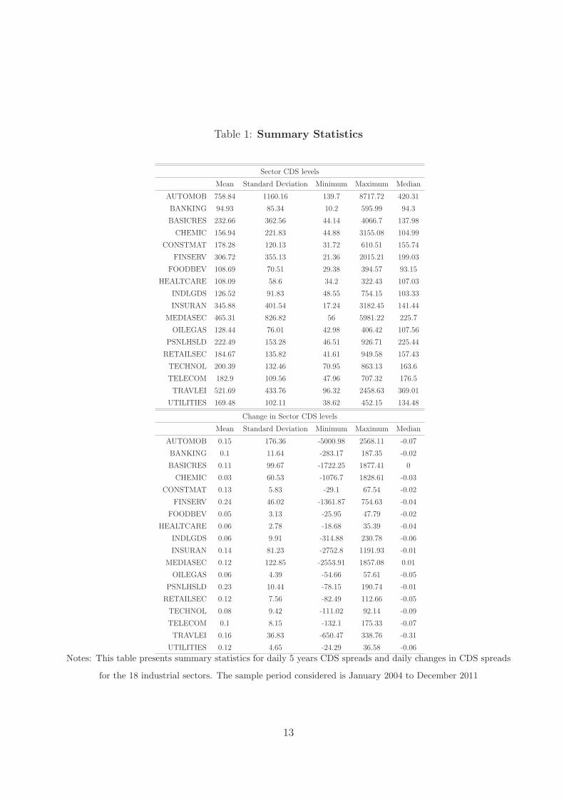
Table 1: Summary Statistics

Sector CDS levels

Mean Standard Deviation Minimum Maximum Median

AUTOMOB 758.84 1160.16 139.7 8717.72 420.31

BANKING 94.93 85.34 10.2 595.99 94.3

BASICRES 232.66 362.56 44.14 4066.7 137.98

CHEMIC 156.94 221.83 44.88 3155.08 104.99

CONSTMAT 178.28 120.13 31.72 610.51 155.74

FINSERV 306.72 355.13 21.36 2015.21 199.03

FOODBEV 108.69 70.51 29.38 394.57 93.15

HEALTCARE 108.09 58.6 34.2 322.43 107.03

INDLGDS 126.52 91.83 48.55 754.15 103.33

INSURAN 345.88 401.54 17.24 3182.45 141.44

MEDIASEC 465.31 826.82 56 5981.22 225.7

OILEGAS 128.44 76.01 42.98 406.42 107.56

PSNLHSLD 222.49 153.28 46.51 926.71 225.44

RETAILSEC 184.67 135.82 41.61 949.58 157.43

TECHNOL 200.39 132.46 70.95 863.13 163.6

TELECOM 182.9 109.56 47.96 707.32 176.5

TRAVLEI 521.69 433.76 96.32 2458.63 369.01

UTILITIES 169.48 102.11 38.62 452.15 134.48

Change in Sector CDS levels

Mean Standard Deviation Minimum Maximum Median

AUTOMOB 0.15 176.36 -5000.98 2568.11 -0.07

BANKING 0.1 11.64 -283.17 187.35 -0.02

BASICRES 0.11 99.67 -1722.25 1877.41 0

CHEMIC 0.03 60.53 -1076.7 1828.61 -0.03

CONSTMAT 0.13 5.83 -29.1 67.54 -0.02

FINSERV 0.24 46.02 -1361.87 754.63 -0.04

FOODBEV 0.05 3.13 -25.95 47.79 -0.02

HEALTCARE 0.06 2.78 -18.68 35.39 -0.04

INDLGDS 0.06 9.91 -314.88 230.78 -0.06

INSURAN 0.14 81.23 -2752.8 1191.93 -0.01

MEDIASEC 0.12 122.85 -2553.91 1857.08 0.01

OILEGAS 0.06 4.39 -54.66 57.61 -0.05

PSNLHSLD 0.23 10.44 -78.15 190.74 -0.01

RETAILSEC 0.12 7.56 -82.49 112.66 -0.05

TECHNOL 0.08 9.42 -111.02 92.14 -0.09

TELECOM 0.1 8.15 -132.1 175.33 -0.07

TRAVLEI 0.16 36.83 -650.47 338.76 -0.31

UTILITIES 0.12 4.65 -24.29 36.58 -0.06

Notes: This table presents summary statistics for daily 5 years CDS spreads and daily changes in CDS spreads

for the 18 industrial sectors. The sample period considered is January 2004 to December 2011

13

Tab

le2:

Correlations

CorrelationMatrix

AUTOMOB

BANKING

BASICRES

CHEMIC

CONSTMAT

FINSERV

FOODBEV

HEALTCARE

INDLGDS

INSURAN

MEDIASEC

OILEGAS

PSNLHSLD

RETAILSEC

TECHNOL

TELECOM

TRAVLEI

UTILITIES

1

BANKIN

G0.11

1

BASIC

RES

0.00

0.04

1

CHEMIC

0.030

0.05

0.02

1

CONSTMAT

0.23

0.30

0.06

0.06

1

FIN

SERV

0.09

0.11

0.07

0.01

0.28

1

FOODBEV

0.17

0.26

0.07

0.06

0.66

0.22

1

HEALTCARE

0.18

0.28

0.05

0.09

0.69

0.2

0.72

1

INDLGDS

0.07

0.14

0.01

0.04

0.28

0.12

0.28

0.29

1

INSURAN

0.05

0.07

0.00

0.02

0.13

0.07

0.09

0.1

0.04

1

MEDIA

SEC

0.08

0.01

-0.13

0.19

0.09

0.03

0.08

0.09

0.06

0.01

1

OILEGAS

0.17

0.26

0.06

0.06

0.65

0.22

0.63

0.63

0.26

0.1

0.07

1

PSNLHSLD

0.24

0.29

0.11

0.18

0.58

0.24

0.53

0.52

0.21

0.1

0.11

0.49

1

RETAILSEC

0.33

0.28

0.05

0.11

0.66

0.23

0.63

0.61

0.22

0.11

0.16

0.53

0.65

1

TECHNOL

0.23

0.25

0.09

0.06

0.57

0.23

0.51

0.53

0.21

0.09

0.11

0.48

0.46

0.53

1

TELECOM

0.17

0.27

0.04

0.07

0.59

0.2

0.6

0.63

0.26

0.1

0.07

0.53

0.51

0.53

0.48

1

TRAVLEI

0.1

0.13

-0.02

0.02

0.31

0.24

0.3

0.27

0.1

0.07

0.11

0.27

0.23

0.32

0.3

0.24

1

UTILIT

IES

0.21

0.28

0.08

0.08

0.68

0.25

0.65

0.68

0.28

0.11

0.09

0.7

0.53

0.57

0.53

0.58

0.27

1

Notes:

Thistable

reportsthecorrelationmatrix

ofdailyCDSindex

changes.Thesample

consistsofdailyobservationsforJanuary

2004to

Decem

ber

2011.

14

Table 3: Summary Statistics of conditioning variables

Conditioning variables levels

Mean St.Dev. Min Max Median

BB-BBB 1.78 0.99 0.52 6.37 1.47

BBB-AAA 1.49 0.9 0.5 4.73 1.41

LIQRISK 0.21 0.19 -0.1 1.72 0.15

NYSE 7649.92 1220.64 4226.31 10311.6 7484.5

RISK-APP 3.14 4 -23.76 26.18 2.92

SP100-PE 19.94 5.5 12.57 40.57 18.5

TBOND5RATE 3.14 1.2 0.79 5.23 3.18

TED 0.51 1.55 -2.04 5.14 0.68

TS 1.89 1.33 -0.62 3.85 2.17

VIX 21.16 10.69 9.89 80.86 18

Changes in conditioning variables

Mean St.Dev. Min Max Median

BB-BBB 0.00 0.07 -0.57 0.6 0

BBB-AAA 0.00 0.06 -1.52 1.53 0

LIQRISK 0.00 0.07 -0.94 0.58 0

NYSE 0.5 99.52 -686.36 696.83 4.13

RISK-APP 0.00 2.5 -26.43 18.67 0.06

SP100-PE -0.01 0.49 -10.31 4.55 0

TBOND5RATE 0.00 0.07 -0.46 0.34 0

TED 0.00 0.07 -0.75 0.82 0

TS 0.00 0.08 -0.49 0.73 0

VIX 0.00 1.96 -17.36 16.54 -0.07

Notes: This table presents summary statistics for the conditioning variables. The sample period considered is

January 2004 to December 2011

15

Tab

le4:

Correlationsbetw

een

conditioningvariablesand

Secto

rCDS

BB-B

BB

BBB-A

AA

LIQ

RISK

NYSE

RISK-A

PP

SP100-P

ETBOND5RATE

TED

TS

VIX

AUTOMOB

0.16

00.03

-0.1

0.06

0-0.08

0.03

-0.05

0.07

BANKIN

G0.21

-0.03

0.05

-0.24

0.18

-0.01

-0.11

0.06

-0.06

0.2

BASIC

RES

0.07

00

-0.05

0.01

0.05

-0.05

0-0.02

0.01

CHEMIC

0.05

-0.04

0.05

-0.02

-0.01

-0.01

-0.04

0.03

-0.01

0.02

CONSTMAT

0.55

0.06

0.08

-0.44

0.3

-0.02

-0.26

0.11

-0.13

0.42

FIN

SERV

0.23

-0.04

0.04

-0.16

0.13

0.01

-0.12

0.06

-0.07

0.15

FOODBEV

0.47

0.08

0.07

-0.36

0.19

-0.02

-0.21

0.1

-0.08

0.31

HEALTCARE

0.52

0.07

0.06

-0.34

0.22

-0.04

-0.22

0.12

-0.08

0.31

INDLGDS

0.21

0.05

0.03

-0.12

0.08

0.02

-0.11

0.03

-0.06

0.09

INSURAN

0.11

-0.01

0.03

-0.1

0.1

0.08

-0.05

0.03

-0.02

0.11

MEDIA

SEC

0.07

-0.02

0.02

0.01

0-0.03

-0.03

0.02

00.01

OILEGAS

0.48

0.09

0.02

-0.32

0.17

0.01

-0.19

0.07

-0.11

0.28

PSNLHSLD

0.41

-0.02

0.05

-0.34

0.22

-0.03

-0.18

0.07

-0.09

0.29

RETAILSEC

0.5

0.01

0.08

-0.37

0.28

-0.05

-0.25

0.09

-0.1

0.33

TECHNOL

0.4

0.02

0.08

-0.26

0.19

-0.04

-0.16

0.11

-0.02

0.25

TELECOM

0.45

00.06

-0.31

0.25

-0.05

-0.18

0.11

-0.06

0.33

TRAVLEI

0.23

0-0.01

-0.12

0.09

-0.02

-0.06

0.02

-0.03

0.13

UTILIT

IES

0.51

0.07

0.07

-0.36

0.22

-0.01

-0.22

0.14

-0.08

0.31

Notes:

This

table

presents

thecorrelationsbetweenthechanges

intheconditioningvariablesandthechanges

intheSectorCDS.Thesample

period

considered

isJanuary

2004to

Decem

ber

2011

16

Tab

le5:

Coefficients

ofth

ecovariatesatdifferentquantiles

Covariates

Quantile

AUTOMOB

BANKING

BASICRES

CHEMIC

CONSTMAT

FINSERV

FOODBEV

HEALTCARE

INDLGDS

INSURAN

MEDIASEC

OILEGAS

PSNLHSLD

RETAILSEC

TECHNOL

TELECOM

TRAVLEI

UTILITIES

BB-B

BB

0.05

1.86

0.21

—0.26

0.39

0.93

0.22

0.23

0.29

0.99

1.04

0.31

0.56

0.46

0.48

0.58

1.62

0.34

0.50

1.55

0.18

0.26

0.25

0.38

0.48

0.17

0.18

0.31

0.42

0.57

0.28

0.48

0.42

0.49

0.52

1.01

0.31

0.95

3.78

0.27

0.41

0.30

0.49

1.42

0.23

0.26

0.38

1.02

1.36

0.35

0.73

0.62

0.65

0.61

1.53

0.41

BBB-A

AA

0.05

——

——

——

——

——

0.60

——

——

——

—

0.50

1.29

—0.18

——

——

——

——

——

——

——

—

0.95

——

——

——

——

——

0.24

——

——

——

—

TS

0.05

-4.33

—-0

.73

-0.34

-0.21

-1.51

-0.11

——

-1.63

-1.27

——

——

——

—

0.50

0.40

——

0.06

——

0.05

0.05

0.02

——

——

——

——

—

0.95

5.78

—1.23

0.73

——

0.23

——

—2.03

0.18

0.57

0.62

0.68

0.14

1.76

—

LIQ

RIS

K0.05

——

——

——

——

——

——

——

——

—-0

.10

0.50

——

——

——

——

——

——

——

——

——

0.95

——

——

——

——

——

——

——

——

——

RIS

K-A

PP

0.05

—0.01

——

——

——

——

——

——

——

——

0.50

——

0.00

—0.00

—0.00

0.00

——

—0.00

——

——

—0.00

0.95

——

-0.02

-0.01

—-0

.02

-0.01

0.00

——

-0.04

-0.01

——

——

—-0

.01

TED

0.05

5.06

0.44

0.87

0.45

—1.77

0.16

—0.31

—1.27

——

—0.33

——

0.28

0.50

——

——

——

——

——

——

——

——

——

0.95

-7.00

—-1

.49

-0.74

——

-0.28

—-0

.28

—-2

.62

-0.21

-0.60

-0.68

-0.70

—-2

.36

—

NYSE

0.05

—-0

.03

——

——

——

—-0

.05

—-0

.01

-0.02

—-0

.02

——

-0.01

0.50

-0.04

-0.01

-0.01

-0.01

-0.01

-0.01

0.00

0.00

-0.01

-0.01

-0.01

0.00

-0.01

-0.01

-0.01

-0.01

-0.02

-0.01

0.95

—-0

.03

—-0

.02

-0.01

——

——

——

—-0

.02

—-0

.02

-0.01

——

TBOND5RATE

0.05

4.10

—0.76

0.40

0.34

1.58

0.22

0.10

0.31

1.79

1.18

0.24

0.41

0.41

0.40

0.57

—0.27

0.50

0.30

—0.10

0.05

0.14

0.17

——

0.11

0.15

0.20

0.11

0.17

0.14

0.13

0.24

0.40

0.09

0.95

—-0

.30

-0.95

-0.52

——

-0.15

——

—-1

.32

——

-0.40

——

——

VIX

0.05

—-0

.01

——

——

——

——

——

——

——

—0.00

0.50

——

0.00

——

——

0.00

—0.01

—0.00

—0.00

—0.00

—0.00

0.95

——

——

0.01

—0.01

0.00

——

—0.01

——

——

—0.01

SP100-P

E0.05

—-0

.01

——

——

——

——

——

——

——

——

0.50

——

——

——

——

——

——

——

——

——

0.95

——

——

——

——

——

——

0.01

——

-0.01

——

Notes:

This

table

presents

thequantile

regressioncoeffi

cients

ofeach

sectorCDSindex

withrespectto

thecovariatesreported

inthefirstcolumn.

Thetable

includes

only

thestatisticallysignificantcoeffi

cients

atthe5%

confiden

celevel.Quantile

levelsare

reported

inthesecondcolumn.The

sample

periodconsidered

isJanuary

2004to

Decem

ber

2011

17

Table 6: Insert text here.

MIN MEAN MEDIAN MAX 25% 75% 5% 95%

0.05 -0.26 0.13 0.11 0.77 -0.04 0.25 -0.15 0.50

0.10 -0.09 0.20 0.15 0.69 0.04 0.35 -0.03 0.56

0.20 0.01 0.27 0.21 0.74 0.13 0.42 0.05 0.60

0.30 0.02 0.31 0.25 0.78 0.16 0.47 0.08 0.62

0.40 0.04 0.33 0.27 0.79 0.17 0.51 0.09 0.66

0.50 0.05 0.34 0.28 0.71 0.18 0.53 0.10 0.68

0.50 0.03 0.35 0.34 0.74 0.20 0.49 0.08 0.67

0.60 0.02 0.33 0.31 0.73 0.19 0.46 0.07 0.65

0.70 0.02 0.31 0.28 0.75 0.16 0.46 0.06 0.61

0.80 0.00 0.28 0.24 0.75 0.13 0.40 0.04 0.58

0.90 -0.08 0.21 0.17 0.75 0.07 0.34 -0.02 0.54

0.95 -0.26 0.16 0.12 0.81 0.01 0.31 -0.12 0.51

Table 7: Insert text here.

BB BBB BBB AAA TS REPO-TBILL RISK APP TED NYSE TBOND5RATE VIX SP100 PE

0.050 0.266 0.225 0.090 -0.197 0.041 0.051 0.001 0.137 0.002 0.174

0.100 0.267 0.244 0.145 0.069 0.166 0.116 0.123 0.139 0.124 0.026

0.200 0.340 0.244 0.125 0.089 0.180 0.110 0.270 0.117 0.172 0.033

0.300 0.340 0.285 0.168 0.102 0.195 0.125 0.295 0.135 0.183 0.042

0.400 0.341 0.300 0.193 0.112 0.220 0.122 0.289 0.134 0.207 0.037

0.500 0.355 0.311 0.182 0.112 0.230 0.124 0.254 0.135 0.226 0.039

0.500 0.395 0.222 0.154 0.106 0.381 0.119 0.229 0.090 0.382 0.071

0.600 0.389 0.201 0.124 0.080 0.350 0.126 0.221 0.101 0.370 0.072

0.700 0.369 0.189 0.126 0.056 0.320 0.095 0.198 0.058 0.342 0.069

0.800 0.347 0.175 0.117 0.033 0.278 0.065 0.155 0.043 0.297 0.062

0.900 0.401 0.135 0.015 0.006 0.217 0.040 0.053 -0.141 0.233 0.171

0.950 0.362 0.131 0.046 -0.077 0.207 0.207 0.007 0.026 0.137 -0.101

18

Tab

le8:

Insert

texthere.

AUTOMOB

BANKIN

GBASIC

RES

CHEMIC

CONSTMAT

FIN

SERV

FOODBEV

HEALTCARE

INDLGDS

INSURAN

MEDIA

SEC

OILEGAS

PSNLHSLD

RETAILSEC

TECHNOL

TELECOM

TRAVLEI

UTILIT

IES

Quan

tile

Coeffi

cient

Coeffi

cient

Coeffi

cient

Coeffi

cient

Coeffi

cient

Coeffi

cient

Coeffi

cient

Coeffi

cient

Coeffi

cient

Coeffi

cient

Coeffi

cient

Coeffi

cient

Coeffi

cient

Coeffi

cient

Coeffi

cient

Coeffi

cient

Coeffi

cient

Coeffi

cient

BB-B

BB

0.05

1.86

0.21

—0.26

0.39

0.93

0.22

0.23

0.29

0.99

1.04

0.31

0.56

0.46

0.48

0.58

1.62

0.34

0.50

1.55

0.18

0.26

0.25

0.38

0.48

0.17

0.18

0.31

0.42

0.57

0.28

0.48

0.42

0.49

0.52

1.01

0.31

0.95

3.78

0.27

0.41

0.30

0.49

1.42

0.23

0.26

0.38

1.02

1.36

0.35

0.73

0.62

0.65

0.61

1.53

0.41

BBB-A

AA

0.05

——

——

——

——

——

0.60

——

——

——

—

0.50

1.29

—0.18

——

——

——

——

——

——

——

—

0.95

——

——

——

——

——

0.24

——

——

——

—

TS

0.05

-4.33

—-0.73

-0.34

-0.21

-1.51

-0.11

——

-1.63

-1.27

——

——

——

—

0.50

0.40

——

0.06

——

0.05

0.05

0.02

——

——

——

——

—

0.95

5.78

—1.23

0.73

——

0.23

——

—2.03

0.18

0.57

0.62

0.68

0.14

1.76

—

LIQ

RISK

0.05

——

——

——

——

——

——

——

——

—-0.10

0.50

——

——

——

——

——

——

——

——

——

0.95

——

——

——

——

——

——

——

——

——

RISK-A

PP

0.05

—0.01

——

——

——

——

——

——

——

——

0.50

——

0.00

—0.00

—0.00

0.00

——

—0.00

——

——

—0.00

0.95

——

-0.02

-0.01

—-0.02

-0.01

0.00

——

-0.04

-0.01

——

——

—-0.01

TED

0.05

5.06

0.44

0.87

0.45

—1.77

0.16

—0.31

—1.27

——

—0.33

——

0.28

0.50

——

——

——

——

——

——

——

——

——

0.95

-7.00

—-1.49

-0.74

——

-0.28

—-0.28

—-2.62

-0.21

-0.60

-0.68

-0.70

—-2.36

—

NYSE

0.05

—-0.03

——

——

——

—-0.05

—-0.01

-0.02

—-0.02

——

-0.01

0.50

-0.04

-0.01

-0.01

-0.01

-0.01

-0.01

0.00

0.00

-0.01

-0.01

-0.01

0.00

-0.01

-0.01

-0.01

-0.01

-0.02

-0.01

0.95

—-0.03

—-0.02

-0.01

——

——

——

—-0.02

—-0.02

-0.01

——

TBOND5R

ATE

0.05

4.10

—0.76

0.40

0.34

1.58

0.22

0.10

0.31

1.79

1.18

0.24

0.41

0.41

0.40

0.57

—0.27

0.50

0.30

—0.10

0.05

0.14

0.17

——

0.11

0.15

0.20

0.11

0.17

0.14

0.13

0.24

0.40

0.09

0.95

—-0.30

-0.95

-0.52

——

-0.15

——

—-1.32

——

-0.40

——

——

VIX

0.05

—-0.01

——

——

——

——

——

——

——

—0.00

0.50

——

0.00

——

——

0.00

—0.01

—0.00

—0.00

—0.00

—0.00

0.95

——

——

0.01

—0.01

0.00

——

—0.01

——

——

—0.01

SP100-PE

0.05

—-0.01

——

——

——

——

——

——

——

——

0.50

——

——

——

——

——

——

——

——

——

0.95

——

——

——

——

——

——

0.01

——

-0.01

——

19

Table 9: Insert text here.

From 2004 From 2007 From 2009

P-value P-value P-value

S AUTOMOB 0.000 0.000 0.003

S BANKING 0.000 0.008 0.001

S BASICRES 0.009 0.166 0.038

S CHEMIC 0.001 0.000 0.047

S CONSTMAT 0.064 0.993 0.252

S FINSERV 0.000 0.002 0.000

S FOODBEV 0.001 0.000 0.047

S HEALTCARE 0.037 0.460 0.000

S INDLGDS 0.003 0.027 0.013

S INSURAN 0.000 0.005 0.676

S MEDIASEC 0.000 0.000 0.432

S OILEGAS 0.019 0.436 0.021

S PSNLHSLD 0.013 0.842 0.352

S RETAILSEC 0.000 0.189 0.002

S TECHNOL 0.010 0.018 0.003

S TELECOM 0.116 0.465 0.000

S TRAVLEI 0.158 0.224 0.014

S UTILITIES 0.003 0.002 0.000

20

Figure 2: Average rolling correlations

21

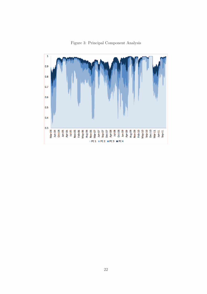
Figure 3: Principal Component Analysis

22

Figure 4: Figure 4a

23

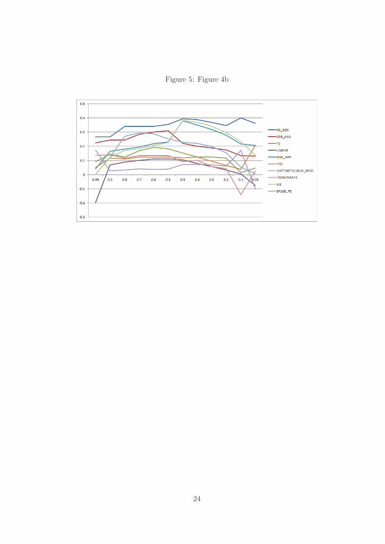
Figure 5: Figure 4b

24

Figure 6: Number quantiles

25