Money Income in the United States: 2001 - Census.gov Income in the United States: 2001 Demographic...

U S C E N S U S B U R E A UHelping You Make Informed Decisions •1902-2002

Issued September 2002

P60-218

Money Income in the United States: 2001

Demographic Programs

ByCarmen DeNavas-WaltRobert W. Cleveland

A

U.S.Department of CommerceEconomics and Statistics Administration

U.S. CENSUS BUREAU

Current Population Reports

Consumer Income

P60

-21

8U

S C E N

S U S B

U R

E A U

Mon

ey In

com

e in th

e Un

ited States: 2

00

1 Cu

rren

t Pop

ula

tion

Rep

orts C

onsu

mer In

come

U.S. Department of CommerceEconomics and Statistics AdministrationU.S. CENSUS BUREAUWashington, DC 20233

OFFICIAL BUSINESS

Penalty for Private Use $300

FIRST-CLASS MAILPOSTAGE & FEES PAIDU.S. Census Bureau

Permit No. G-58

This report was prepared under the direction of Edward J. Welniak Jr., Chief of the Income Surveys Branch. Shane L. Martinmade significant contributions to the preparation of this report.Shirley L. Smith and Diana Marz provided statistical assistance.Ruth E. Davis and Doris Sansbury provided clerical assistance.Charles T. Nelson, Assistant Division Chief for Income, Poverty,and Health Statistics, Housing and Household Economic StatisticsDivision, provided overall direction.

David Nguyen and John Dinh, Demographic Surveys Division,processed the March 2002 Annual Demographic Supplement CurrentPopulation Survey file. Caroline S. Carbaugh, Chief of the SurveyProcessing Branch, Stacy J. Lyons, Mary Thrift Bush, and Kirk E.Davis programmed the detailed tables.

Aneesah Stephenson and Fred Meier of the DemographicStatistical Methods Division conducted sampling review.

Tim J. Marshall, Demographic Surveys Division, and Andrew M.Stevenson, Technologies Management Office, prepared and pro-grammed the computer-assisted interviewing instrument used toconduct the Annual Demographic Supplement.

U.S. Census Bureau field representatives and telephone interviewerscollected the data. Without their dedication, the preparation of thisreport or any report from the Current Population Survey would beimpossible.

Greg Carroll, Penny Heiston, Jan Sweeney, and Mary Stinsonof the Administrative and Customer Services Division, Walter C.Odom, Chief, provided publications and printing management,graphics design and composition, and editorial review for print andelectronic media. General direction and production managementwere provided by Gary J. Lauffer, Chief, Publications ServicesBranch.

AcknowledgmentsThe Housing and Household Economic Statistics Division of theCensus Bureau recognizes Shirley L. Smith for her 31 years ofservice with the Census Bureau. Ms. Smith spent the last 28years working on income data collected in current surveys andthree decennial censuses. One particularly noteworthy accom-plishment is the extensive series of historical tables availableon our web site. Her dedication, professionalism, and institu-tional knowledge will be sorely missed.

U.S. Department of CommerceDonald L. Evans,

Secretary

Samuel W. Bodman,Deputy Secretary

Economics and Statistics AdministrationKathleen B. Cooper,

Under Secretary for Economic Affairs

U.S. CENSUS BUREAUCharles Louis Kincannon,

Director

Money Income in theUnited States: 2001

P60-218

Issued September 2002

Suggested Citation

DeNavas-Walt, Carmen and RobertCleveland, U.S. Census Bureau,

Current Population Reports, P60-218, Money Income in the United States:

2001, U.S. Government PrintingOffice, Washington, DC,

2002.

ECONOMICS

AND STATISTICS

ADMINISTRATION

Economics and StatisticsAdministration

Kathleen B. Cooper,Under Secretary for Economic Affairs

U.S. CENSUS BUREAU

Charles Louis Kincannon,Director

William G. Barron, Jr.,Deputy Director

Vacant,Principal Associate Director for Programs

Nancy M. Gordon,Associate Director for Demographic Programs

Daniel H. Weinberg,Chief, Housing and Household EconomicStatistics Division

For sale by the Superintendent of Documents, U.S. Government Printing Office

Internet: bookstore.gpo.gov Phone: toll-free 866-512-1800; DC area 202-512-1800

Fax: 202-512-2250 Mail: Stop SSOP, Washington, DC 20402-0001

U.S. Census Bureau Money Income in the United States: 2001 iii

TEXT

Introduction . . . . . . . . . . . . . . . . . . . . . . . . . . . . . . . . . . . . . . . . . 1

Highlights . . . . . . . . . . . . . . . . . . . . . . . . . . . . . . . . . . . . . . . . . . 1

Official Estimates of Money Income . . . . . . . . . . . . . . . . . . . . . . . . 2

Experimental Estimates of Income Including Noncash Benefits and Taxes . . . . . . . . . . . . . . . . . . . . . . . . . . . . . . . . . . . 9

User Comments . . . . . . . . . . . . . . . . . . . . . . . . . . . . . . . . . . . . . . 14

TEXT TABLES

1. Comparison of Summary Measures of Income by SelectedCharacteristics: 2000 and 2001 . . . . . . . . . . . . . . . . . . . . . . 4

2. Income of Households by Race and Hispanic Origin Using 2- and 3-Year-Average Medians . . . . . . . . . . . . . . . . . . . 6

3. Distribution of Households by Selected Characteristics Within Income Quintiles: 2001 . . . . . . . . . . . . . . . . . . . . . . . 10

4. Income of Households by State Using 2- and 3-Year-Average Medians . . . . . . . . . . . . . . . . . . . . . . . . . . . . . . 11

5. Median Household Income by Definition: 2000 and 2001 . . . . . 13

6. Percentage of Aggregate Income Received by Income Quintiles and Gini Index by Definition of Income: 2001 . . . . . 14

FIGURES

1. Median Household Income by Race and Hispanic Origin: 1967 to 2001 . . . . . . . . . . . . . . . . . . . . . . . . . . . . . . 5

2. Median Earnings of Full-Time, Year-Round Workers 15 Years Old and Over by Sex: 1967 to 2001 . . . . . . . . . . . . 7

3. Index of Change for Various Measures of Household Income Inequality: 1967 to 2001 . . . . . . . . . . . . . . . . . . . . . 8

4. Percent Change in 2-Year-Average Median Household Income by State: 1999-2000 to 2000-2001 . . . . . . . . . . . . . . 12

Appendix A. HISTORICAL INCOME

A-1. Households by Total Money Income, Race, and Hispanic Origin of Householder: 1967 to 2001 . . . . . . . . 15

A-2. Share of Aggregate Income Received by Each Fifth and Top 5 Percent of Households: 1967 to 2001 . . . . . . . . . . 19

A-3. Selected Measures of Household Income Dispersion: 1967 to 2001 . . . . . . . . . . . . . . . . . . . . . . . . . . . . . . . . . 20

Contents

iv Money Income in the United States: 2001 U.S. Census Bureau

Appendix B. SAMPLE EXPANSION AND INTRODUCTION OF CENSUS 2000-BASED POPULATION CONTROLS

B-1. Comparison of 2000 Median Income Using the Expanded Sample and the Original Sample by Selected Characteristics . . . . . . . . . . . . . . . . . . . . . . . . . . 25

B-2. Comparison of 2000 Median Income by State Using the Expanded Sample and the Original Sample . . . . . . . . . . . . . . . . . . . . . . . . . . . . . . . . . . . . . . . . . . . 26

B-3. Comparison of 2000 Median Income Using Census 2000-Based Population Controls and 1990 Census-Based Population Controls by Selected Characteristics . . . . . . . . . . . . . . . . . . . . . . . . . . . . . . . . . . . . . . . . . 27

INTRODUCTION

The 2001 median householdincome in the United States was$42,228, representing a 2.2 per-cent decline in real income from its2000 level of $43,162.1 Thisdecline in income coincides withthe recession that started in March2001.2 The decline in medianhousehold income between 2000and 2001 was widespread. Withthe exception of the Northeast, allregions experienced a decline in

income. Each of the racial groupsand non-Hispanic Whites showeddeclines in income; the income ofthe Hispanic population remainedunchanged.3

HIGHLIGHTS

(Most of the estimates described inthis section are shown in Table 1,Table 2, Table 3, and AppendixTable A-1; the estimates for statesare shown in Table 4.)

• Real median household incomedeclined by 2.2 percent between2000 and 2001 to a level of$42,228.

• The real median income of familyhouseholds and of nonfamilyhouseholds declined between2000 and 2001. Overall, familyhousehold income dropped 1.7percent to $52,275. Nonfamilyhouseholds experienced a declineof 1.5 percent, to $25,631.4

• Foreign-born households experi-enced a 5.3 percent decline inmedian income between 2000and 2001 (to $37,948), largerthan the 1.5 percent decline (to$42,917) experienced by nativehouseholds.5

U.S. Census Bureau Money Income in the United States: 2001 1

Money Income in the United States: 2001

The estimates in this report are based on the 2000,2001, and 2002 Current Population Survey AnnualDemographic Supplements (CPS ADS) and provideinformation for calendar years 1999, 2000, and2001, respectively. These estimates use populationestimates based on Census 2000. Earlier reportspresenting data for calendar years 1993 through2000 used population estimates based on the 1990census.

In 2001, the Census Bureau tested a sample expan-sion of 28,000 households to the CPS ADS. Thesample expansion was officially implemented in theestimates presented here. It is primarily designed to

improve the reliability of state estimates of children’shealth insurance coverage, but the larger samplesize also improves the reliability of national esti-mates of other topics.

Because results presented in this report from the2001 survey have been recalculated based on theexpanded sample and the Census 2000-basedweights, they may differ from earlier estimates thatdid not incorporate the sample expansion and werebased on the 1990 census. Appendix B presentsmore detail on the introduction of the sample expan-sion and new population controls based on Census2000.

NEW POPULATION CONTROLS AND EXPANDED SAMPLE

1 All income values are in 2001 dollars.Changes in real income refer to comparisonsafter adjusting for inflation. The percentagechanges in prices between earlier years and2001 were computed by dividing the annualaverage Consumer Price Index for 2001 bythe annual average for earlier years. TheCPI-U values for 1947 to 2001 are availableon the Internet at:www.census.gov/hhes/www/income01.html;click on “Annual Average Consumer PriceIndex (CPI-U-RS): 1947 to 2001.” Inflationbetween 2000 and 2001 was 2.8 percent.

2 Recessions are determined by theNational Bureau of Economic Research, a pri-vate research organization.

3 Because Hispanics may be of any race,data in this report for Hispanics overlapslightly with data for the Black populationand the Asian and Pacific Islander popula-tion. About 10.9 percent of White house-holds, 3.0 percent of Black households, 2.0percent of Asian and Pacific Islander house-holds, and 13.1 percent of American Indianand Alaska Native households are main-tained by a person of Hispanic origin.

4 The percent declines in median incomefor family and nonfamily households are notdifferent.

5 Native households are those in whichthe householder was born in the UnitedStates, Puerto Rico, or an outlying area ofthe United States or was born in a foreigncountry but had at least one parent who wasa U.S. citizen. All other households are con-sidered foreign-born regardless of the dateof entry into the United States or citizenshipstatus. The CPS does not interview house-holds in Puerto Rico.

• While the real median income ofHispanic-origin householdsremained unchanged between2000 and 2001 ($33,565), theincome of each race groupdeclined. Median householdincome declined 1.3 percent fornon-Hispanic Whites, 3.4 percentfor Blacks, and 6.4 percent forAsians and Pacific Islanders.6

• The Northeast was the onlyregion that did not experience adecline in real median householdincome between 2000 and 2001.

• Real median income declined forhouseholds in metropolitanareas between 2000 and 2001,going to a level of $45,219.

• The real median earnings ofwomen who worked full-time,

year-round increased for thefifth consecutive year, rising to$29,215. Men with similar workexperience did not experience astatistical change in earnings($38,275). As a result, thefemale-to-male earnings ratioreached 0.76, up from the previ-ous all-time-high of 0.74, firstrecorded in 1996.

• The most commonly used indexof household income inequality,the Gini index, did not changebetween 2000 and 2001, whilethe share of aggregate incomereceived by the lowest house-hold income quintile declined.

• Based on comparisons of 2-year-average medians (comparing1999-2000 with 2000-2001), realmedian household income rosefor 3 states (Arizona,Massachusetts, andPennsylvania) and declined for12 states. Five of the states that

experienced declines were in theMidwest (Illinois, Indiana, Iowa,Michigan, and Wisconsin), four inthe South (Alabama, Florida,Mississippi, and Tennessee), twoin the Northeast (Maine andVermont), and one in the West(Washington).

• An important finding of theCensus Bureau’s tax and noncashbenefit research is that govern-ment transfers have a greaterimpact on lowering incomeinequality than the tax system.

OFFICIAL ESTIMATES OFMONEY INCOME

The official income estimates in thisreport are based solely on moneyincome before taxes and do notinclude the value of employment-based fringe benefits nor of govern-ment-provided noncash benefits,such as food stamps, medicare,medicaid, and public or subsidizedhousing. A separate section of thisreport, “Experimental Estimates ofIncome Including Noncash Benefitsand Taxes,” discusses the effect oftaxes and selected noncash benefitson household income using model-based approaches to estimatingtaxes and valuing benefits. TheCensus Bureau’s models of theseeffects are based on informationcollected in the 2002 CPS AnnualDemographic Supplement and othersources, including the InternalRevenue Service, the Food andNutrition Service, the Bureau ofLabor Statistics, and the Centers forMedicare and Medicaid Services.7

Median household incomedeclined between 2000 and2001.

Real median household incomedeclined by 2.2 percent between

2 Money Income in the United States: 2001 U.S. Census Bureau

6 The differences between the percentdeclines in the median income of Blackhouseholds compared with that of non-Hispanic White and Asian and Pacific Islanderhouseholds are not statistically significant.

What is . . .? Money Income data are collected for all people inthe sample 15 years old and over. Money income includes earnings,unemployment compensation, workers’ compensation, social securi-ty, supplemental security income, public assistance, veterans’ pay-ments, survivor benefits, pension or retirement income, interest, divi-dends, rents, royalties, estates, trusts, educational assistance,alimony, child support, assistance from outside the household, andother miscellaneous money income. It is income before deductionsfor taxes or other expenses and does not include lump-sum pay-ments or capital gains.

7 See Current Population Reports, SeriesP60-186RD, “Measuring the Effect of Benefitsand Taxes on Income and Poverty: 1992,” formore details.

Source of Estimates; Statistical Accuracy

The estimates in this report are based on data collected by the 2002Current Population Survey Annual Demographic Supplement conduct-ed by the U.S. Census Bureau. As with all surveys, the estimatesmay differ from the actual values because of sampling variation orother factors. All statements in this report have undergone statisticaltesting, and all comparisons are significant at the 90-percent confi-dence level unless otherwise noted. For further information aboutthe source and accuracy of the estimates, go to www.census.gov/hhes/income/income01/sa.pdf.

2000 ($43,162) and 2001($42,228), coinciding with therecession that started in March2001. The last time householdincome declined was in 1991,which also coincided with a reces-sion that lasted from July 1990 toMarch 1991 (see Table 1 andAppendix Table A-1).

Family and nonfamilyhouseholds experienceddeclines in median householdincome.

The real median income of familyhouseholds declined between 2000and 2001 (see Table 1). The dropfor family household medianincome overall was 1.7 percent to$52,275; for those maintained byfemale householders with no hus-band present 3.1 percent to$28,142; and for those with malehouseholders with no wife present6.0 percent to $40,715. The per-centage decline in income of non-family households was 1.5 percentto $25,631.8 The income ofmarried-couple families remainedunchanged at $60,471.

Family and nonfamily householdshave not experienced declines inreal median household income sincethe early 1990s. Specifically, familyhouseholds had not experienced anannual decline in real medianincome since 1993, family house-holds maintained by women with nohusband present since 1991, andfamily households maintained bymen with no wife present and non-family households since 1992.

Native and foreign-bornhouseholds experienceddeclines in real medianhousehold income between2000 and 2001.

Foreign-born households experi-enced a 5.3 percent decline (to$37,948) in real median householdincome, larger than the 1.5 percentdecline (to $42,917) experiencedby native households (see Table 1).Of foreign-born households, thosemaintained by a naturalized citizenexperienced a 5.4 percent declinein income (to $43,968), not differ-ent from the 4.2 percent decline(to $34,812) for those maintainedby householders who were notUnited States citizens.9

The real median income ofHispanic-origin householdsremained unchanged between2000 and 2001, but theincome of each of the racegroups declined. 10

Hispanic households had a medianincome of $33,565 in 2001, notstatistically different from their2000 median income (see Table 1).Before 2001, Hispanic householdshad experienced 5 years of annualincome increases (see AppendixTable A-1). Their last decline inmedian household incomeoccurred in 1995.

The real median incomes of non-Hispanic White, Black, and Asianand Pacific Islander householdsdeclined between 2000 and 2001,by 1.3 percent (to $46,305) fornon-Hispanic White households; by3.4 percent (to $29,470) for Blackhouseholds; and by 6.4 percent (to$53,635) for Asian and PacificIslander households. 11 12

Non-Hispanic White and Asian andPacific Islander households havenot experienced an annual declinein median household income since1991 and Black households since1981 (see Appendix Table A-1).

Although Asians and PacificIslanders as a group had the high-est median household income in2001, their income per householdmember ($24,933) was not statisti-cally different from the income perhousehold member of non-Hispanic White households($25,751). Asian and PacificIslander households typically havemore people—2.93 people on aver-age compared with 2.42 people fornon-Hispanic White households.The income per household mem-ber for Black households (averagesize of 2.68 people) was $14,635and for Hispanic households (aver-age size of 3.52) was $12,595.13

Table 2 shows income data for theAmerican Indian and Alaska Native


8 The percentage declines in medianincome for family households, nonfamilyhouseholds, and households maintained byfemales with no husband present are not dif-ferent. The percentage decline in medianincome for households maintained by afemale with no husband present is not dif-ferent from the percentage declines for non-family households and households main-tained by males with no wife present.

11 Data users should exercise cautionwhen interpreting aggregate results for theAsian and Pacific Islander (API) populationbecause the API population consists of manydistinct groups that differ in socio-economiccharacteristics, culture, and recency of immi-gration. In addition, the CPS does not useseparate population controls for weightingthe API sample to national totals.

12 The differences between the percentdeclines in the median household income ofBlacks compared with that of non-HispanicWhite and Asian and Pacific Islander house-holds are not statistically significant.

13 For a discussion of standardizingincome by size of family using the officialpoverty thresholds, see Current PopulationReports, Series P60-219, “Poverty in theUnited States: 2001.”

9 The median household income of nativehouseholds was not different from the medi-an for households maintained by a natural-ized citizen. The difference between per-centage changes for households withnoncitizen householders and householdswith native, foreign-born, and naturalizedcitizens were not statistically significant. Inaddition, the differences between the per-centage change for foreign-born householdsand those with a naturalized householderwas not significant.

10 Data users should exercise cautionwhen interpreting aggregate results for theHispanic population because this populationconsists of many distinct groups that differin socio-economic characteristics, culture,and recency of immigration. Data were firstcollected for Hispanics in 1972.


Table 1.Comparison of Summary Measures of Income by Selected Characteristics: 2000 and 2001(Households and people as of March of the following year. For meaning of symbols, see text)

Characteristic

2001Median income in 20001

(in 2001 dollars)

Percentchange in

real income2000 to

2001

90-percentconfidence

interval2 (±)of percent

changeNumber

(thousands)

Median income

Value(dollars)


interval2 (±)(dollars)

Value(dollars)



HOUSEHOLDSAll households . . . . . . . . . . . . . . . . . . . . . . . . . . . 109,297 42,228 212 43,162 223 *–2.2 0.6

Type of HouseholdFamily households . . . . . . . . . . . . . . . . . . . . . . . . . . 74,329 52,275 290 53,155 304 *–1.7 0.6

Married-couple families . . . . . . . . . . . . . . . . . . . . 56,747 60,471 342 60,926 453 –0.7 0.8Female householder, no husband present . . . . . 13,143 28,142 475 29,053 516 *–3.1 1.9Male householder, no wife present . . . . . . . . . . . 4,438 40,715 860 43,332 854 *–6.0 2.2

Nonfamily households . . . . . . . . . . . . . . . . . . . . . . . 34,969 25,631 278 26,012 279 *–1.5 1.2Female householder . . . . . . . . . . . . . . . . . . . . . . . 19,390 20,264 347 21,052 323 *–3.7 1.8Male householder . . . . . . . . . . . . . . . . . . . . . . . . . 15,579 32,312 395 32,358 358 –0.1 1.3

Race and Hispanic Origin of HouseholderAll races3. . . . . . . . . . . . . . . . . . . . . . . . . . . . . . . . 109,297 42,228 212 43,162 223 *–2.2 0.6

White. . . . . . . . . . . . . . . . . . . . . . . . . . . . . . . . . . . . . 90,682 44,517 344 45,142 328 *–1.4 0.8Non-Hispanic White . . . . . . . . . . . . . . . . . . . . . . . 80,818 46,305 316 46,896 309 *–1.3 0.8

Black . . . . . . . . . . . . . . . . . . . . . . . . . . . . . . . . . . . . . 13,315 29,470 571 30,495 665 *–3.4 2.3Asian and Pacific Islander . . . . . . . . . . . . . . . . . . . . 4,071 53,635 2,106 57,313 1,608 *–6.4 3.7

Hispanic origin4 . . . . . . . . . . . . . . . . . . . . . . . . . . . . 10,499 33,565 701 34,094 808 –1.6 2.1

Age of HouseholderUnder 65 years. . . . . . . . . . . . . . . . . . . . . . . . . . . . . 86,821 49,227 327 49,990 338 *–1.5 0.8

15 to 24 years. . . . . . . . . . . . . . . . . . . . . . . . . . . . 6,391 28,196 799 28,624 656 –1.5 2.925 to 34 years. . . . . . . . . . . . . . . . . . . . . . . . . . . . 18,988 45,080 614 45,654 712 –1.3 1.735 to 44 years. . . . . . . . . . . . . . . . . . . . . . . . . . . . 24,031 53,320 689 55,263 619 *–3.5 1.345 to 54 years. . . . . . . . . . . . . . . . . . . . . . . . . . . . 22,208 58,045 801 59,251 747 *–2.0 1.555 to 64 years. . . . . . . . . . . . . . . . . . . . . . . . . . . . 15,203 45,864 699 46,105 742 –0.5 1.865 years and over. . . . . . . . . . . . . . . . . . . . . . . . . 22,476 23,118 314 23,727 294 *–2.6 1.4

Nativity of the HouseholderNative born . . . . . . . . . . . . . . . . . . . . . . . . . . . . . . . . 95,884 42,917 339 43,578 250 *–1.5 0.8Foreign born . . . . . . . . . . . . . . . . . . . . . . . . . . . . . . . 13,413 37,948 943 40,055 977 *–5.3 2.7

Naturalized citizen . . . . . . . . . . . . . . . . . . . . . . . . 6,069 43,968 1,513 46,492 1,409 *–5.4 3.5Not a citizen . . . . . . . . . . . . . . . . . . . . . . . . . . . . . 7,344 34,812 872 36,345 827 *–4.2 2.6

RegionNortheast . . . . . . . . . . . . . . . . . . . . . . . . . . . . . . . . . 21,128 45,716 615 44,971 720 1.7 1.7Midwest. . . . . . . . . . . . . . . . . . . . . . . . . . . . . . . . . . . 25,755 43,834 574 45,496 560 *–3.7 1.4South . . . . . . . . . . . . . . . . . . . . . . . . . . . . . . . . . . . . 39,151 38,904 507 39,460 473 *–1.4 1.4West . . . . . . . . . . . . . . . . . . . . . . . . . . . . . . . . . . . . . 23,263 45,087 740 46,169 666 *–2.3 1.7

ResidenceInside metropolitan areas. . . . . . . . . . . . . . . . . . . . . 88,112 45,219 309 45,942 342 *–1.6 0.8

Inside central cities . . . . . . . . . . . . . . . . . . . . . . . . 32,540 36,731 347 37,741 387 *–2.7 1.1Outside central cities . . . . . . . . . . . . . . . . . . . . . . 55,572 50,697 337 51,606 358 *–1.8 0.8

Outside metropolitan areas . . . . . . . . . . . . . . . . . . . 21,185 33,601 604 33,832 692 –0.7 2.2

EARNINGS OF FULL-TIME,YEAR-ROUND WORKERS

Male . . . . . . . . . . . . . . . . . . . . . . . . . . . . . . . . . . . . . 58,712 38,275 424 38,292 171 - -Female . . . . . . . . . . . . . . . . . . . . . . . . . . . . . . . . . . . 41,639 29,215 271 28,228 172 *3.5 1.0

PER CAPITA INCOMEAll races3. . . . . . . . . . . . . . . . . . . . . . . . . . . . . . . . 282,082 22,851 174 22,970 193 –0.5 0.9

White. . . . . . . . . . . . . . . . . . . . . . . . . . . . . . . . . . . . . 230,071 24,127 202 24,240 230 –0.5 1.0Non-Hispanic White . . . . . . . . . . . . . . . . . . . . . . . 194,822 26,134 234 26,242 265 –0.4 1.1

Black . . . . . . . . . . . . . . . . . . . . . . . . . . . . . . . . . . . . . 36,023 14,953 308 15,209 348 –1.7 2.4Asian and Pacific Islander . . . . . . . . . . . . . . . . . . . . 12,500 24,277 1,124 24,002 1,146 1.1 5.2

Hispanic origin4 . . . . . . . . . . . . . . . . . . . . . . . . . . . . 37,438 13,003 326 13,004 402 - -

*Statistically significant change at the 90-percent confidence level.1Consistent with 2001 data through implementation of Census 2000-based population controls and a 28,000 household sample expansion.2For an explanation of confidence intervals, see ‘‘Standard errors and their use’’ at www.census.gov/hhes/income/income01/sa.pdf.3Data for American Indians and Alaska Natives are not shown separately in this table because of the small sample of those households.4Hispanics may be of any race.

Source: U.S. Census Bureau, Current Population Survey, 2002 and 2001 Annual Demographic Supplements.

population.14 Because of the smallsize of this racial group, samplingvariability of income data is largerthan for the other racial groupsand causes single-year estimates tofluctuate more widely. To reducethe chances of misinterpretingchanges in income or comparisonof income with other groups, theCensus Bureau uses 2-year-averagemedians for evaluating changes inthe income of American Indiansand Alaska Natives over time, and

3-year-average medians when com-paring the income of this groupwith other racial and ethnic origingroups.15 These 2- and 3-year-average medians make the esti-mates less volatile.

The 3-year-average (1999-2001)median household income forAmerican Indians and AlaskaNatives was $32,116, higher thanthe 3-year-average for Blacks($29,870), not statistically differentfrom that for Hispanics ($33,439),but lower than for non-HispanicWhites ($46,702) and Asians andPacific Islanders ($55,026) (seeTable 2). Based on comparisons of2-year-average medians (1999-2000


Figure 1.Median Household Income by Race and Hispanic Origin: 1967 to 20011

1Hispanics may be of any race. Data for Hispanics not available before 1972. Data for Asians and Pacific Islanders not available before 1987.Source: U.S. Census Bureau, Current Population Survey, 1968 to 2002 Annual Demographic Supplements.

Income in 2001 dollars Recession

$53,635

$29,470

0

10000

20000

30000

40000

50000

60000

2001 1997 1994 1991 1988 1985 1982 1979 1976 1973 19701967

$46,305

$44,517

$33,565

Asian and Pacific Islander

Non-Hispanic White

Hispanic origin

White

Black

14 Data users should exercise cautionwhen interpreting aggregate results for theAmerican Indian and Alaska Native (AIAN)population because the AIAN population con-sists of groups that differ in economic char-acteristics. Data from the 1990 census showthat the median income of AIAN householdsliving on reservations or in Alaska Native vil-lages was $18,466 (in 2001 dollars) com-pared with $30,521 (in 2001 dollars) forhouseholds outside those areas. In addition,the CPS does not use separate populationcontrols for weighting the AIAN sample tonational totals.

15 The 2-year-average median is the sumof 2 inflation adjusted single-year mediansdivided by 2. The 3-year-average median isthe sum of 3 inflation adjusted single-yearmedians divided by 3.

Detailed Tabulations

Detailed tabulations that pro-vide income of households,families, and people 15 years ofage and older are available onthe Internet at:www.census.gov/hhes/www/income.html.

Income data are cross-tabulat-ed by various characteristicssuch as age, sex, race,Hispanic origin, presence ofchildren, marital status, educa-tional attainment, work experi-ence, occupation, class ofworker, and source of income.Historical data are available aswell. The historical tablesshow income data for house-holds, families, and people byvarious characteristics.

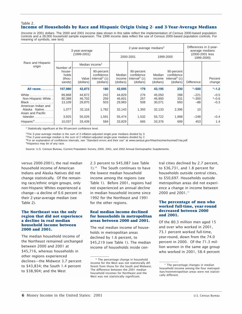
versus 2000-2001), the real medianhousehold income of AmericanIndians and Alaska Natives did notchange statistically. Of the remain-ing race/ethnic origin groups, onlynon-Hispanic Whites experienced achange—a decline of 0.6 percent intheir 2-year-average median (seeTable 2).

The Northeast was the onlyregion that did not experiencea decline in real medianhousehold income between2000 and 2001.

The median household income ofthe Northeast remained unchangedbetween 2000 and 2001 at$45,716, whereas households inother regions experienceddeclines—the Midwest 3.7 percentto $43,834; the South 1.4 percentto $38,904; and the West

2.3 percent to $45,087 (see Table1).16 The South continues to havethe lowest median householdincome among the regions (seeTable 1). Before 2001, regions hadnot experienced an annual declinein median household income since1992 for the Northeast and 1991for the other regions.

Real median income declinedfor households in metropolitanareas between 2000 and 2001.

The real median income of house-holds in metropolitan areasdeclined by 1.6 percent, to$45,219 (see Table 1). The medianincome of households inside cen-

tral cities declined by 2.7 percent,to $36,731, and 1.8 percent forhouseholds outside central cities,to $50,697. Households outsidemetropolitan areas did not experi-ence a change in income between2000 and 2001.17

The percentage of men whoworked full-time, year-rounddecreased between 2000 and 2001.

Of the 80.3 million men aged 15and over who worked in 2001,73.1 percent worked full-time,year-round, down from the 74.0percent in 2000. Of the 71.3 mil-lion women in the same age groupwho worked in 2001, 58.4 percent


Table 2.Income of Households by Race and Hispanic Origin Using 2- and 3-Year-Average Medians(Income in 2001 dollars. The 2000 and 2001 income data shown in this table reflect the implementation of Census 2000-based populationcontrols and a 28,000 household sample expansion. The 1999 income data reflect the use of Census 2000-based population controls. Formeaning of symbols, see text)

Race and Hispanicorigin

3-year-average(1999-2001)

2-year-average medians2 Differences in 2-year-average medians(2000-2001 less

1999-2000)2000-2001 1999-2000

Number ofhouse-

holds(thou-

sands)

Median income1

Medianincome

(dollars)



Medianincome

(dollars)


interval3 (±)(dollars) Difference

Percentchange

Value(dollars)



All races . . . . . . . . 107,980 42,873 180 42,695 179 43,195 230 *–500 *–1.2

White . . . . . . . . . . . . . . . 89,868 44,872 242 44,829 276 45,050 288 –221 –0.5Non-Hispanic White . 80,388 46,702 259 46,601 257 46,900 331 *–300 *–0.6

Black . . . . . . . . . . . . . . . 13,109 29,870 503 29,983 508 30,071 650 –88 –0.3American Indian and

Alaska Native. . . . . . 1,077 32,116 1,782 32,143 1,393 32,133 2,396 10 -Asian and Pacific

Islander . . . . . . . . . . . . 3,925 55,026 1,591 55,474 1,532 55,722 1,998 –248 –0.4

Hispanic4. . . . . . . . . . . . 10,037 33,439 584 33,829 665 33,376 699 453 1.4

* Statistically significant at the 90-percent confidence level.

1The 3-year-average median is the sum of 3 inflation-adjusted single-year medians divided by 3.2The 2-year-average median is the sum of 2 inflation-adjusted single-year medians divided by 2.3For an explanation of confidence intervals, see ‘‘Standard errors and their use’’ at www.census.gov/hhes/income/income01/sa.pdf.4Hispanics may be of any race.

Source: U.S. Census Bureau, Current Population Survey, 2000, 2001, and 2002 Annual Demographic Supplements.

16 The percentage change in householdincome for the West was not statistically dif-ferent from those for the South and Midwest.The difference between the 2001 medianhousehold incomes for Northeast and theWest was not statistically significant.

17 The percentage changes in medianhousehold income among the four metropol-itan/nonmetropolitan areas were not statisti-cally different.

worked full-time, year-round—unchanged from 2000.

The real median earnings ofwomen who worked full-time,year-round increased for thefifth consecutive year.

Between 2000 and 2001, the medi-an earnings of women who workedfull-time, year-round increased by3.5 percent, to $29,215 (see Table1). Men with similar work experi-ence did not experience a statisticalchange in earnings between 2000and 2001 ($38,275), or between1999 and 2000, but experiencedannual increases for each of theprevious 3 years. This dissimilarpattern in the annual changes inearnings of men and women con-tributed to a rise in the female-to-male earnings ratio. In 2001, theearnings ratio reached 0.76, upfrom the previous all-time-high of0.74, first recorded in 1996.

Per capita income remainedstatistically unchanged.

The per capita income of the over-all population, of each of the racegroups, and of Hispanics, remainedunchanged between 2000 and2001 (see Table 1). In 2001, percapita income was $22,851 for theoverall population, $26,134 fornon-Hispanic Whites, $24,277 forAsians and Pacific Islanders,$14,953 for Blacks, and $13,003for Hispanics.

The Gini index indicated nochange in household incomeinequality between 2000 and2001.

The Gini index has not shown anannual change since 1993.Comparisons with earlier years arenot recommended because of asubstantial methodological changein the 1994 CPS Annual


What are . . .? Full-time,Year-round workersworked 50 or more weeksand 35 or more hours perweek during the calendaryear. Paid vacations arecounted as time worked.

Figure 2.Median Earnings of Full-Time, Year-Round Workers 15 Years Old and Over by Sex: 1967 to 2001

Source: U.S. Census Bureau, Current Population Survey, 1968 to 2002 Annual Demographic Supplements.

Earnings in 2001 dollars Recession

$38,275

$29,215

0

5,000

10,000

15,000

20,000

25,000

30,000

35,000

40,000

2001 1997 1994 1991 1988 1985 1982 1979 1976 1973 1970 1967

Female, full-time, year-round workers

Male, full-time, year-round workers

What is . . .? Earnings con-sists of: gross money wage orsalary income, including com-missions, tips and cashbonuses, before deductions;net income from nonfarmself-employment (grossreceipts minus businessexpenses); and net incomefrom farm self-employment(gross receipts minus farmexpenses).

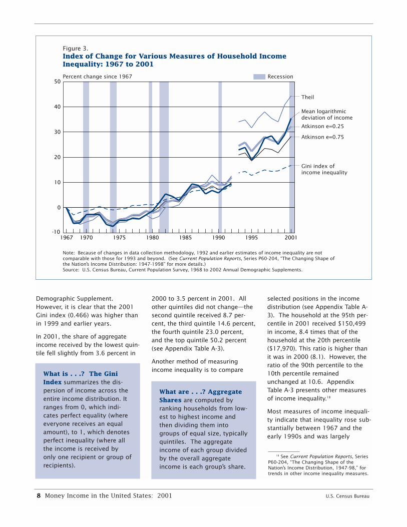
Demographic Supplement.However, it is clear that the 2001Gini index (0.466) was higher thanin 1999 and earlier years.

In 2001, the share of aggregateincome received by the lowest quin-tile fell slightly from 3.6 percent in

2000 to 3.5 percent in 2001. Allother quintiles did not change—thesecond quintile received 8.7 per-cent, the third quintile 14.6 percent,the fourth quintile 23.0 percent,and the top quintile 50.2 percent(see Appendix Table A-3).

Another method of measuringincome inequality is to compare

selected positions in the incomedistribution (see Appendix Table A-3). The household at the 95th per-centile in 2001 received $150,499in income, 8.4 times that of thehousehold at the 20th percentile($17,970). This ratio is higher thanit was in 2000 (8.1). However, theratio of the 90th percentile to the10th percentile remainedunchanged at 10.6. Appendix Table A-3 presents other measuresof income inequality.18

Most measures of income inequali-ty indicate that inequality rose sub-stantially between 1967 and theearly 1990s and was largely


What is . . .? The GiniIndex summarizes the dis-persion of income across theentire income distribution. Itranges from 0, which indi-cates perfect equality (whereeveryone receives an equalamount), to 1, which denotesperfect inequality (where allthe income is received byonly one recipient or group ofrecipients).

What are . . .? AggregateShares are computed byranking households from low-est to highest income andthen dividing them intogroups of equal size, typicallyquintiles. The aggregateincome of each group dividedby the overall aggregateincome is each group’s share.

Figure 3.Index of Change for Various Measures of Household Income Inequality: 1967 to 2001

Note: Because of changes in data collection methodology, 1992 and earlier estimates of income inequality are not comparable with those for 1993 and beyond. (See Current Population Reports, Series P60-204, “The Changing Shape of the Nation’s Income Distribution: 1947-1998” for more details.) Source: U.S. Census Bureau, Current Population Survey, 1968 to 2002 Annual Demographic Supplements.

Percent change since 1967

Atkinson e=0.25

-10

0

10

20

30

40

50

20011995199019851980197519701967

Gini index of income inequality

Atkinson e=0.75

Theil

Mean logarithmic deviation of income

Recession

18 See Current Population Reports, SeriesP60-204, “The Changing Shape of theNation’s Income Distribution, 1947-98,” fortrends in other income inequality measures.

unchanged through the late 1990s(see Figure 3).19

High-income householdstended to be family householdsthat included two or moreearners, lived in the suburbs ofa large city, and had a workinghouseholder between 35 and54 years old. In contrast, low-income households tendedto be in a city with an elderlyhouseholder who lived aloneand did not work.

The 20 percent of households withthe highest income (the highestquintile) received at least $83,500during 2001. The lowest 20 per-cent of households (the lowestquintile) received less than$17,970 during 2001.

Half of households in the top quin-tile lived in a metropolitan areaoutside a city of 1 million or morepeople (see Table 3). Only 10.4percent lived outside any metro-politan area. Among households inthe lowest income quintile, aboutone-quarter (24.5 percent) lived ina metropolitan area outside a cityof 1 million or more, and one-quarter (24.9 percent) livedoutside a metropolitan area.20

Nearly 9 out of 10 households(87.3 percent) in the top quintilewere family households while 8out of 10 (79.9 percent) were mar-ried-couple households. Amonglow-income households, onlyabout 4 out of 10 (40.8 percent)were family households, and only2 out of 10 (19.6 percent) weremarried-couple households.

A high-income household in 2001tended to have a householder in hisor her peak earning years— about 6out of 10 householders (59.5 per-cent) were between 35 and 54 yearsold. Among low-income households,only one-quarter of householders(25.0 percent) were between 35 and54, and the largest proportion (39.7percent) were over 65 years old.

Most high-income households(78.0 percent) had two or moreearners contributing to householdincome while only 2.6 percent ofhouseholds in the top quintile hadno earners. Among low-incomehouseholds, the majority (59.4 per-cent) had no earners, and 6.1 per-cent had two or more.

The majority of high-incomehouseholds (73.7 percent) had ahouseholder who worked full-time,year-round; only 10.4 percent ofhigh-income households had anonworking householder. Amonglow-income households, mosthouseholders (64.7 percent) didnot work in 2001, and 13.5 per-cent worked full-time, year-round.

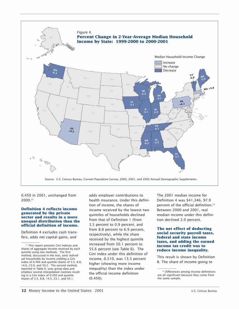
Real median householdincome rose for 3 states anddeclined for 12 states.

Based on comparisons of 2-year-average medians (comparing 1999-2000 with 2000-2001), real medianhousehold income rose for 3 states(Arizona, Massachusetts, andPennsylvania) and declined for 12states (see Table 4 and Figure 4).21

Five of the states that experienceddeclines were in the Midwest(Illinois, Indiana, Iowa, Michigan,and Wisconsin), four in the South(Alabama, Florida, Mississippi, andTennessee), two in the Northeast

(Maine and Vermont), and one inthe West (Washington).

Comparing the relative ranking ofstates using 3-year-average medi-ans for 1999-2001 shows that themedian household income forAlaska, although not statisticallydifferent from the median incomesfor Maryland, Connecticut, andMinnesota, was higher than thatfor the remaining 46 states and theDistrict of Columbia. Conversely,the median household income forWest Virginia, although notstatistically different from themedian for Arkansas, was lowerthan the incomes of the remaining48 states and the District ofColumbia. The relative standing ofthe remaining states and theDistrict of Columbia was less clearbecause of sampling variabilitysurrounding the estimates.

EXPERIMENTAL ESTIMATESOF INCOME INCLUDINGNONCASH BENEFITS AND TAXES

Traditionally, income data presentedin the Census Bureau’s reports havebeen based on the amount ofmoney received during a calendaryear before taxes and excludingcapital gains, but this restricted def-inition of income does not provide acompletely satisfactory measure ofincome. Over time, tax laws maychange and affect the economicwell-being of the population. In theearly 1980s, the Census Bureauembarked on a research program toexamine the effects of taxes on eco-nomic well being. Four types ofmodeled tax data are included here:federal individual income taxes,state individual income taxes, prop-erty taxes on owner-occupied hous-ing, and payroll taxes.

Because noncash benefits increasethe income resources available toindividuals and families, this report


21 To reduce the possibilities of misinter-preting changes in, or rankings of, incomeestimates for states, the Census Bureau uses2-year-average medians for evaluatingchanges in state estimates over time, and 3-year-average medians when comparing therelative ranking of states.

19 A change in data collection methodolo-gy in 1993 affected income measurement andoverstated the increase in income inequalitythat year. See Paul Ryscavage, “A Surge inGrowing Income Inequality?,” Monthly LaborReview, August 1995, pp. 51-61.

20 The difference between the percent ofhouseholds living in suburbs and the percentliving outside of a metropolitan area was notstatistically significant.

also presents income measuresthat include the valuation of vari-ous noncash benefits, such as foodstamps, school lunches, housingsubsidies, medicare, medicaid,employer contributions to healthinsurance, and net imputed returnson home equity.22

Taxes, government transfers,and other benefits affect thedistribution and the level ofincome.

As shown in Table 5, there was adecline in real income between

2000 and 2001 for 13 (definitions1-13) of the 15 definitions ofincome (only a few of which arediscussed below).

Definition 1, the official definitionof income, is based on moneyincome before taxes and includesgovernment cash transfers.Between 2000 and 2001, realmedian income of householdsdeclined, 2.2 percent, to $42,228.Under Definition 1, the share ofaggregate household incomereceived by each quintile was 3.5percent for the lowest, 8.8 percentfor the second, 14.5 percent forthe third, 23.1 percent for thefourth, and 50.1 percent for thehighest. The Gini index for allhouseholds under Definition 1 was


Table 3.Distribution of Households by Selected Characteristics Within Income Quintiles: 2001(Households as of March 2002)

Characteristic Lowest quintile Middle three quintiles Highest quintile

Type of Residence . . . . . . . . . . . . . . . . . . . . . . . . . . . . . . . . . . . . . . . . . . . . 100.0 100.0 100.0

Inside metropolitan area. . . . . . . . . . . . . . . . . . . . . . . . . . . . . . . . . . . . . . . . . 75.1 79.5 89.6Inside central cities . . . . . . . . . . . . . . . . . . . . . . . . . . . . . . . . . . . . . . . . . . . 36.4 29.3 24.6Outside central cities . . . . . . . . . . . . . . . . . . . . . . . . . . . . . . . . . . . . . . . . . 38.7 50.2 65.0

Metropolitan area of 1 million or more . . . . . . . . . . . . . . . . . . . . . . . . 24.5 33.6 50.2Metropolitan area under 1 million. . . . . . . . . . . . . . . . . . . . . . . . . . . . . 14.2 16.6 14.8

Outside metropolitan area . . . . . . . . . . . . . . . . . . . . . . . . . . . . . . . . . . . . . . . 24.9 20.5 10.4

Type of Household . . . . . . . . . . . . . . . . . . . . . . . . . . . . . . . . . . . . . . . . . . . . 100.0 100.0 100.0

Family households . . . . . . . . . . . . . . . . . . . . . . . . . . . . . . . . . . . . . . . . . . . . . 40.8 70.6 87.3Married-couple families . . . . . . . . . . . . . . . . . . . . . . . . . . . . . . . . . . . . . . . 19.6 53.4 79.9Other families . . . . . . . . . . . . . . . . . . . . . . . . . . . . . . . . . . . . . . . . . . . . . . . . 21.2 17.3 7.4

Nonfamily households . . . . . . . . . . . . . . . . . . . . . . . . . . . . . . . . . . . . . . . . . . 59.2 29.4 12.7Householder living alone . . . . . . . . . . . . . . . . . . . . . . . . . . . . . . . . . . . . . . 55.9 23.1 6.5

Age of Householder . . . . . . . . . . . . . . . . . . . . . . . . . . . . . . . . . . . . . . . . . . . 100.0 100.0 100.0

15 to 34 years . . . . . . . . . . . . . . . . . . . . . . . . . . . . . . . . . . . . . . . . . . . . . . . . . 21.9 25.9 16.435 to 54 years . . . . . . . . . . . . . . . . . . . . . . . . . . . . . . . . . . . . . . . . . . . . . . . . . 25.0 42.3 59.555 to 64 years . . . . . . . . . . . . . . . . . . . . . . . . . . . . . . . . . . . . . . . . . . . . . . . . . 13.4 13.4 16.265 years or older . . . . . . . . . . . . . . . . . . . . . . . . . . . . . . . . . . . . . . . . . . . . . . . 39.7 18.4 7.9

Number of Earners . . . . . . . . . . . . . . . . . . . . . . . . . . . . . . . . . . . . . . . . . . . . 100.0 100.0 100.0

No earners . . . . . . . . . . . . . . . . . . . . . . . . . . . . . . . . . . . . . . . . . . . . . . . . . . . . 59.4 13.9 2.6One earner . . . . . . . . . . . . . . . . . . . . . . . . . . . . . . . . . . . . . . . . . . . . . . . . . . . . 34.5 41.0 19.4Two or more earners . . . . . . . . . . . . . . . . . . . . . . . . . . . . . . . . . . . . . . . . . . . 6.1 45.2 78.0

Work Experience of Householder . . . . . . . . . . . . . . . . . . . . . . . . . . . . . . 100.0 100.0 100.0

Worked . . . . . . . . . . . . . . . . . . . . . . . . . . . . . . . . . . . . . . . . . . . . . . . . . . . . . . . 35.3 76.1 89.6Worked full-time, year-round . . . . . . . . . . . . . . . . . . . . . . . . . . . . . . . . . . . 13.5 56.7 73.7Worked part-time or part-year. . . . . . . . . . . . . . . . . . . . . . . . . . . . . . . . . . 21.7 19.4 15.8

Did not work . . . . . . . . . . . . . . . . . . . . . . . . . . . . . . . . . . . . . . . . . . . . . . . . . . . 64.7 23.9 10.4

Source: U.S. Census Bureau, Current Population Survey, 2002 Annual Demographic Supplement.

Model-Based StateEstimates

The Census Bureau also com-putes improved (in the sense ofhaving lower standard errors)annual estimates of medianhousehold income for states,as well as biennial estimatesfor counties, based on modelsusing data from the CPS, the1990 decennial census, andadministrative records. State-level estimates for 1998 areavailable on the Internet at:www.census.gov/hhes/www/saipe.html. Estimates forincome year 1999 will be avail-able later this fall.

22 For more information on the methodol-ogy and procedures used to estimate taxesand to value noncash benefits see CurrentPopulation Reports, P60-186RD, “Measuringthe Effect of Benefits and Taxes on Incomeand Poverty: 1992.”


Table 4.Income of Households by State Using 2- and 3-Year-Average Medians(Income in 2001 dollars. The 2000 income data used in this table reflect the implementation of Census 2000-based population controls anda 28,000 household sample expansion. The 1999 income data reflect the use of Census 2000-based population controls)

State

3-year-average median1

1999-2001

2-year-average medians2

2000-2001 average less1999-2000 average

2000-2001 1999-2000

Medianincome

(dollars)



Medianincome

(dollars)



Medianincome

(dollars)


interval3 (±)(dollars) Difference

Percentchange

United States . . . . . 42,873 180 42,695 179 43,195 230 *–500 *–1.2Alabama. . . . . . . . . . . . 36,693 1,294 35,786 1,425 37,460 1,600 *–1,673 *–4.5Alaska . . . . . . . . . . . . . 55,426 2,103 55,842 2,199 54,458 2,465 1,385 2.5Arizona. . . . . . . . . . . . . 40,965 1,489 41,799 1,817 40,095 1,654 *1,704 *4.2Arkansas . . . . . . . . . . . 31,798 1,146 31,932 1,320 31,027 1,280 905 2.9California . . . . . . . . . . . 47,243 834 47,692 968 47,233 981 459 1.0Colorado . . . . . . . . . . . 50,053 1,549 49,492 1,664 50,380 1,929 –889 –1.8Connecticut . . . . . . . . . 52,887 1,979 52,460 1,782 52,657 2,636 –197 –0.4Delaware . . . . . . . . . . . 50,301 2,099 50,686 2,040 50,650 2,716 36 0.1District of Columbia . . . 41,539 1,476 41,771 1,436 41,724 1,913 47 0.1Florida . . . . . . . . . . . . . 38,141 732 38,181 814 39,000 967 *–820 *–2.1

Georgia . . . . . . . . . . . . 42,508 1,281 42,823 1,306 42,474 1,574 349 0.8Hawaii . . . . . . . . . . . . . 49,232 1,700 50,212 1,677 50,129 2,170 83 0.2Idaho . . . . . . . . . . . . . . 38,310 1,430 38,451 1,486 38,344 1,847 107 0.3Illinois. . . . . . . . . . . . . . 47,578 1,140 46,760 1,266 48,281 1,410 *–1,521 *–3.1Indiana . . . . . . . . . . . . . 41,921 1,352 41,192 1,118 42,692 1,786 –1,500 *–3.5Iowa . . . . . . . . . . . . . . . 42,255 1,199 41,556 1,336 42,895 1,385 –1,339 *–3.1Kansas. . . . . . . . . . . . . 41,097 1,764 41,810 1,565 40,938 2,351 872 2.1Kentucky . . . . . . . . . . . 37,184 1,325 37,857 1,272 36,557 1,687 1,300 3.6Louisiana . . . . . . . . . . . 33,194 1,274 32,449 1,392 33,130 1,485 –682 –2.1Maine . . . . . . . . . . . . . . 38,733 1,236 37,459 1,236 39,793 1,559 *–2,334 *–5.9

Maryland . . . . . . . . . . . 55,013 2,079 54,794 2,091 55,755 2,600 –962 –1.7Massachusetts. . . . . . . 49,018 1,935 50,155 1,969 47,400 2,421 *2,755 *5.8Michigan . . . . . . . . . . . 46,929 1,195 45,915 1,353 47,869 1,497 *–1,955 *–4.1Minnesota . . . . . . . . . . 52,804 1,765 54,223 1,971 52,865 2,280 1,358 2.6Mississippi . . . . . . . . . . 33,305 1,570 32,709 1,745 34,877 1,952 *–2,169 *–6.2Missouri . . . . . . . . . . . . 43,884 1,414 43,847 1,638 45,157 1,680 –1,309 –2.9Montana. . . . . . . . . . . . 32,929 1,086 32,909 1,201 33,330 1,389 –422 –1.3Nebraska . . . . . . . . . . . 42,518 1,379 43,263 1,462 41,972 1,698 1,291 3.1Nevada . . . . . . . . . . . . 45,493 1,556 46,219 1,466 45,538 2,007 681 1.5New Hampshire. . . . . . 50,866 1,640 51,839 1,374 50,634 2,295 1,205 2.4

New Jersey . . . . . . . . . 52,137 1,328 51,791 1,319 52,320 1,711 –529 –1.0New Mexico. . . . . . . . . 34,599 1,681 34,598 1,704 35,337 2,137 –738 –2.1New York . . . . . . . . . . . 42,157 819 41,998 809 42,179 1,046 –181 –0.4North Carolina . . . . . . . 39,040 1,065 38,774 1,204 39,479 1,252 –705 –1.8North Dakota . . . . . . . . 35,830 1,314 36,397 1,290 35,848 1,741 549 1.5Ohio . . . . . . . . . . . . . . . 42,631 951 42,973 956 43,053 1,226 –80 –0.2Oklahoma . . . . . . . . . . 34,554 1,186 34,473 959 34,027 1,613 446 1.3Oregon. . . . . . . . . . . . . 42,701 1,184 42,479 1,163 43,416 1,558 –937 –2.2Pennsylvania . . . . . . . . 42,320 1,025 43,426 978 41,730 1,328 *1,696 *4.1Rhode Island . . . . . . . . 44,825 1,665 44,549 1,483 44,376 2,185 173 0.4

South Carolina. . . . . . . 38,362 1,479 38,177 1,342 38,675 1,935 –497 –1.3South Dakota. . . . . . . . 38,407 974 38,582 1,058 37,775 1,163 807 2.1Tennessee . . . . . . . . . . 36,542 1,218 35,415 1,183 36,921 1,599 *–1,506 *–4.1Texas . . . . . . . . . . . . . . 40,547 948 40,273 902 40,391 1,284 –118 –0.3Utah . . . . . . . . . . . . . . . 48,378 1,657 48,110 1,822 48,896 1,907 –787 –1.6Vermont . . . . . . . . . . . . 41,888 1,302 40,747 1,278 42,435 1,670 *–1,689 *–4.0Virginia. . . . . . . . . . . . . 49,085 1,587 49,360 1,516 48,508 2,044 853 1.8Washington . . . . . . . . . 44,835 1,823 43,101 1,695 46,007 2,378 *–2,906 *–6.3West Virginia . . . . . . . . 30,342 990 29,952 903 30,676 1,299 –723 –2.4Wisconsin . . . . . . . . . . 46,734 1,583 45,846 1,422 47,427 2,065 – 1,581 *–3.3Wyoming . . . . . . . . . . . 40,007 1,379 40,227 1,522 40,150 1,661 77 0.2

* Statistically significant at the 90-percent confidence level.1The 3-year-average median is the sum of 3 inflation-adjusted single-year medians divided by 3.2The 2-year-average median is the sum of 2 inflation-adjusted single-year medians divided by 2.3For an explanation of confidence intervals, see ‘‘Standard errors and their use’’ at www.census.gov/hhes/income/income01/sa.pdf.



0.450 in 2001, unchanged from2000.23

Definition 4 reflects incomegenerated by the privatesector and results in a moreunequal distribution than theofficial definition of income.

Definition 4 excludes cash trans-fers, adds net capital gains, and

adds employer contributions tohealth insurance. Under this defini-tion of income, the shares ofincome received by the lowest twoquintiles of households declinedfrom that of Definition 1 (from 3.5 percent to 0.9 percent, andfrom 8.8 percent to 6.9 percent,respectively), while the sharereceived by the highest quintileincreased from 50.1 percent to55.6 percent (see Table 6). TheGini index under this definition ofincome, 0.510, was 13.3 percenthigher (showing more incomeinequality) than the index underthe official income definition(0.450).

The 2001 median income forDefinition 4 was $41,346, 97.9percent of the official definition.24

Between 2000 and 2001, realmedian income under this defini-tion declined 2.0 percent.

The net effect of deductingsocial security payroll taxes,federal and state incometaxes, and adding the earnedincome tax credit was toreduce income inequality.

This result is shown by Definition8. The share of income going to

TX

NM

WA-6.3

NV

MI-4.1

IL-3.1

MO

MT

WY

ID

UTCO

HI

NE

AK

KS

OK

WI-3.3

IA-3.1

LA

ME-5.9

VT-4.0

IN-3.5

KY

TN-4.1

AL-4.5

GA

OH

WV

NC

SC

NJMD

CTRI

MA +5.8

DE

SD

VA

AR

CA

AZ+4.2

NY

DC

OR

PA+4.1

ND

MN

MS-6.2

FL-2.1

NH

IncreaseNo changeDecrease

Median Household Income Change

Figure 4. Percent Change in 2-Year-Average Median Household Income by State: 1999-2000 to 2000-2001


24 Differences among income definitionsare all significant because they come fromthe same sample.

23 This report presents Gini indexes andshares of aggregate income received by eachquintile using two methods. The firstmethod, discussed in the text, sorts individ-ual households by income yielding a Giniindex of 0.466 and quintile shares of 3.5, 8.8,14.6, 23.0, and 50.2. The second method,reported in Table 6, uses group data andemploys several interpolation routines result-ing in a Gini index of 0.450 and quintileshares of 3.5, 8.8, 14.5, 23.1, and 50.1.

the bottom three quintilesincreased, and the share receivedby the highest quintile declined.The Gini index was 0.492, or 3.5 percent below the value of0.510 for Definition 4.

The 2001 median income forDefinition 8 was $34,927, 82.7percent of the official definition.Between 2000 and 2001, realmedian income declined 1.6 per-cent under Definition 8.

Nonmeans-tested cashtransfers reduced incomeinequality more than taxes.

Nonmeans-tested cash transfers,such as social security, lowered theGini index by 13.4 percent, from0.492 to 0.426, as shown by com-paring Definition 11 estimates withDefinition 8 estimates. Includingthe benefits increased the share of

income going to the lowest quin-tile (from 1.2 percent to 3.9 per-cent) and lowered the share goingto the highest quintile (from 51.8percent to 47.7 percent).

The 2001 median income underDefinition 11 was $40,653, 96.3percent of the official definition.Between 2000 and 2001, realmedian income declined 0.6 per-cent for Definition 11.

Means-tested noncashtransfers also reduced incomeinequality, as shown byDefinition 14.

When means-tested noncash trans-fers were included, the share ofincome in the lowest quintileincreased (from 3.9 percent to 4.5percent) while the share in thehighest quintile decreased (from47.7 percent to 47.0 percent). The

Gini index declined 3.3 percentfrom 0.426 to 0.412.25

The 2001 median income forDefinition 14 was $41,533, 98.4percent of the official definition.Between 2000 and 2001, realmedian income did not changeunder this definition of income.

An important finding of theCensus Bureau’s tax andnoncash benefit research isthat government transfershave a greater impact onlowering income inequalitythan the tax system.

In 2001, subtracting taxes andincluding the earned income credit(EIC) lowered the Gini index by


Table 5.Median Household Income by Definition: 2000 and 2001(Income in 2001 dollars)

Definition of incomeMedian income

Percent change2001-2000

Percent ofofficial definition

of income22001 2000

Income before taxes:

1. Money income excluding capital gains (official measure). . . . . . 42,228 43,162 *–2.2 100.02. Definition 1 less government cash transfers . . . . . . . . . . . . . . . . . 39,010 39,811 *–2.0 92.43. Definition 2 plus capital gains . . . . . . . . . . . . . . . . . . . . . . . . . . . . . 39,561 40,427 *–2.1 93.74. Definition 3 plus health insurance supplements to wage or

salary income . . . . . . . . . . . . . . . . . . . . . . . . . . . . . . . . . . . . . . . . . . 41,346 42,209 *–2.0 97.9

Income after taxes:

5. Definition 4 less social security payroll taxes . . . . . . . . . . . . . . . . 38,773 39,546 *–2.0 91.86. Definition 5 less federal income taxes (excluding the EIC) . . . . 35,885 36,458 *–1.6 85.07. Definition 6 plus the earned income credit (EIC)1 . . . . . . . . . . . . 36,072 36,628 *–1.5 85.48. Definition 7 less state income taxes . . . . . . . . . . . . . . . . . . . . . . . . 34,927 35,495 *–1.6 82.79. Defintion 8 plus nonmeans-tested government cash transfers . 38,628 39,062 *–1.1 91.510. Definition 9 plus the value of medicare . . . . . . . . . . . . . . . . . . . . . 40,635 40,903 *–0.7 96.211. Definition 10 plus the value of regular-price school lunches . . . 40,653 40,918 *–0.6 96.312. Definition 11 plus means-tested government cash transfers . . . 40,819 41,115 *–0.7 96.713. Definition 12 plus the value of medicaid . . . . . . . . . . . . . . . . . . . . 41,373 41,517 –0.3 98.014. Definition 13 plus the value of other means-tested

government noncash transfers . . . . . . . . . . . . . . . . . . . . . . . . . . . 41,533 41,654 –0.3 98.415. Definition 14 plus net imputed return on equity in own home . . 43,237 (NA) (NA) 102.4

* Statistically significant at the 90-percent confidence level. NA Not available.

1 Thirteen states (Colorado, Illinois, Iowa, Kansas, Maine, Maryland, Massachusetts, New Jersey, New York, Oregon, Rhode Island, Vermont,and Wisconsin) and District of Columbia have an EIC that uses federal eligibility rules to compute the state credit. The remaining states do not have state EIC.

2 Differences between income definitions are all significant because they come from the same sample.

Source: U.S. Census Bureau, Current Population Survey, 2001 and 2002 Annual Demographic Supplements.

25 There was no change in incomeinequality between 2000 and 2001 using themost comprehensive definition of income.However, the 2001 Gini index for definition14 is higher than in 1997.

3.5 percent (from 0.510 to 0.492),while including transfers loweredthe Gini index by 16.3 percent(from 0.492 to 0.412).

CPS Data Collection

The information in this report wascollected in the 50 states and theDistrict of Columbia and does notinclude residents of Puerto Ricoand outlying areas. The estimatesin this report are controlled tonational population estimates byage, race, sex, and Hispanic origin,and to state population estimatesby age, and are based on the newexpanded CPS sample. For moreinformation on the CPS expansion,see Appendix B. The populationcontrols used to prepare the esti-mates in this report are based onresults of Census 2000.

The CPS excludes armed forcespersonnel living on military basesand people living in institutions.For further documentation aboutthe CPS Annual DemographicSupplement, seewww.bls.census.gov/cps/ads/adsmain.htm.

Rounding

The Census Bureau rounds percent-ages to the nearest tenth of a per-cent; therefore, the percentages ina distribution do not always sumto exactly 100.0 percent.

Symbols Used in Tables

- Represents zero or rounds tozero.

B Base less than 75,000.NA Not available.r Revised.X Not applicable.

USER COMMENTS

The Census Bureau welcomes thecomments and advice of users ofdata and reports. If you have anysuggestions or comments, pleasewrite to:

Edward J. Welniak, Jr.Chief, Income Surveys BranchHousing and Household Economic

Statistics DivisionU.S. Census BureauWashington, DC 20233-8500

[email protected]


What are . . .? GovernmentCash Transfers includesocial security, railroad retire-ment, black lung, unemploy-ment compensation, workers’compensation, veterans’ bene-fits, government educationalassistance, cash public assis-tance, and supplemental secu-rity income.

Table 6.Percentage of Aggregate Income Received by Income Quintiles and Gini Indexby Definition of Income: 2001

Definition of incomeQuintiles

Gini indexLowest Second Third Fourth Highest

Definition 1 (official measure) . . . . . . . . . . . . . . . . . . . . . . . . . . 3.5 8.8 14.5 23.1 50.1 .450Definition 4 (definition 1 less government cash transfers

plus capital gains and employee health benefits) . . . . . . . . 0.9 6.9 13.7 22.8 55.6 .510Definition 8 (definition 4 less taxes, plus EIC) . . . . . . . . . . . . . 1.2 8.1 15.0 23.9 51.8 .492Definition 11 (definition 8 plus nonmeans tested

government cash transfers, value of medicare, and valueof regular-price school lunches) . . . . . . . . . . . . . . . . . . . . . . . 3.9 10.0 15.6 22.8 47.7 .426

Definition 14 (definition 11 plus means-tested governmentcash transfers, value of medicaid, and value of othermeans-tested government noncash transfers) . . . . . . . . . . . 4.5 10.3 15.6 22.6 47.0 .412

Definition 15 (definition 14 plus return on home equity) . . . . 4.7 10.4 15.6 22.7 46.5 .407


What are . . .? Nonmeans-tested Cash Transfersinclude social security, rail-road retirement, black lung,unemployment compensation,workers’ compensation, non-means-tested veterans’ bene-fits, and government educa-tional assistance.

What are . . .? Means-testedCash Transfers include cashpublic assistance, supplementalsecurity income, and means-tested veterans’ benefits.


Table A-1.Households by Total Money Income, Race, and Hispanic Origin of Householder:1967 to 2001(Income in 2001 CPI-U-RS adjusted dollars. Households as of March of the following year. For meaning of symbols, see text)

Race andHispanic originof householder

and year Number(thou-

sands)

Percent distribution Median income Mean income

TotalUnder

$5,000

$5,000to

$9,999

$10,000to

$14,999

$15,000to

$24,999

$25,000to

$34,999

$35,000to

$49,999

$50,000to

$74,999

$75,000to

$99,999$100,000and over

Value(dol-lars)

Stan-darderror(dol-lars)

Value(dol-lars)

Stan-darderror

(dollars)

ALL RACES

2001 . . . . . . . 109,297 100.0 3.1 5.9 6.9 13.3 12.4 15.4 18.4 10.8 13.8 42,228 129 58,208 2322000 1 . . . . . . 108,209 100.0 2.9 5.8 6.9 13.0 12.5 15.4 18.6 10.8 14.1 43,162 136 58,730 2252000 2 . . . . . . 106,418 100.0 2.8 5.9 6.8 13.1 12.5 15.1 18.9 10.8 14.1 43,327 202 58,639 3281999 . . . . . . . 104,705 100.0 2.7 5.8 7.0 13.3 12.3 15.5 18.6 10.8 14.0 43,355 204 58,254 3051998 . . . . . . . 103,874 100.0 3.0 6.3 7.0 13.4 12.6 15.4 18.7 10.7 12.7 42,173 249 56,240 3041997 . . . . . . . 102,528 100.0 3.1 6.7 7.3 13.9 12.5 16.0 18.5 10.2 11.8 40,699 188 54,653 3061996 . . . . . . . 101,018 100.0 3.0 7.0 7.8 14.2 13.0 15.6 18.8 9.9 10.8 39,869 201 52,934 2971995 3 . . . . . . 99,627 100.0 3.1 6.9 7.8 14.5 12.9 16.3 18.4 9.8 10.3 39,306 227 51,835 2841994 4 . . . . . . 98,990 100.0 3.3 7.5 7.8 14.8 12.7 16.4 17.9 9.5 10.0 38,119 174 50,961 2741993 5 . . . . . . 97,107 100.0 3.6 7.7 7.9 14.4 13.3 16.4 17.9 9.2 9.7 37,688 176 49,977 270

1992 6 . . . . . . 96,426 100.0 3.5 7.8 7.9 14.7 12.9 16.5 18.6 9.1 9.0 37,880 179 48,024 2021991 . . . . . . . 95,669 100.0 3.1 7.8 7.5 14.3 13.6 16.7 18.7 9.4 9.0 38,183 184 48,064 1981990 . . . . . . . 94,312 100.0 3.1 7.5 7.3 13.9 13.3 17.3 18.9 9.4 9.2 39,324 201 49,121 2081989 . . . . . . . 93,347 100.0 2.9 7.3 7.2 14.1 12.8 16.8 19.3 9.7 9.8 39,850 219 50,347 2191988 . . . . . . . 92,830 100.0 3.0 7.8 7.3 14.1 12.6 16.8 19.6 9.7 9.0 39,144 191 48,910 2191987 7 . . . . . . 91,124 100.0 3.2 7.9 7.4 14.0 13.1 16.8 19.3 9.6 8.7 38,835 185 48,297 1981986 . . . . . . . 89,479 100.0 3.5 8.0 7.3 14.5 12.9 17.2 19.0 9.4 8.3 38,365 199 47,398 1931985 8 . . . . . . 88,458 100.0 3.4 8.1 7.7 14.6 13.9 17.2 18.7 9.1 7.3 37,059 201 45,607 1801984 . . . . . . . 86,789 100.0 3.3 8.2 8.0 15.1 13.8 17.6 18.6 8.5 6.9 36,343 165 44,530 1641983 9 . . . . . . 85,290 100.0 3.5 8.3 8.0 15.5 14.3 17.6 18.6 8.0 6.2 35,438 160 43,179 160

1982 . . . . . . . 83,918 100.0 3.5 8.6 8.3 15.4 13.7 18.7 18.2 7.8 5.9 35,423 160 42,690 1581981 . . . . . . . 83,527 100.0 3.2 8.7 8.1 15.8 13.6 18.1 19.1 7.8 5.5 35,478 186 42,384 1541980 . . . . . . . 82,368 100.0 3.0 8.5 8.2 15.2 13.9 18.4 19.4 7.8 5.6 36,035 185 42,857 1571979 10 . . . . . 80,776 100.0 2.9 8.4 7.6 14.9 13.7 18.3 20.2 8.0 6.0 37,192 176 44,181 1671978 . . . . . . . 77,330 100.0 2.7 8.4 8.0 14.9 13.6 18.6 20.0 8.1 5.7 37,234 151 43,824 1681977 . . . . . . . 76,030 100.0 2.9 8.9 8.5 15.5 14.2 18.9 19.4 7.0 4.7 34,989 131 41,506 1261976 11 . . . . . 74,142 100.0 3.0 9.0 8.3 15.9 14.2 19.6 19.0 6.8 4.3 34,792 129 40,924 1261975 12 . . . . . 72,867 100.0 3.1 9.2 8.6 15.8 15.0 19.4 18.6 6.3 4.0 34,219 139 39,958 1251974 13 12 . . . 71,163 100.0 3.0 8.8 7.8 15.2 15.4 19.5 19.1 6.9 4.4 35,159 135 41,116 1291973 . . . . . . . 69,859 100.0 3.5 8.0 8.1 14.7 14.6 19.5 19.7 7.1 4.8 36,278 138 41,955 128

1972 14 . . . . . 68,251 100.0 3.9 8.4 7.9 14.6 14.8 20.2 19.1 6.6 4.6 35,560 136 41,387 1281971 15 . . . . . 66,676 100.0 4.5 8.8 7.5 15.4 15.5 20.9 17.8 5.8 3.7 34,126 132 39,248 1251970 . . . . . . . 64,778 100.0 4.6 8.6 7.4 15.0 15.4 21.5 18.0 5.9 3.7 34,481 126 39,483 1261969 . . . . . . . 63,401 100.0 4.6 8.5 7.2 14.8 15.8 21.7 18.3 5.6 3.6 34,714 128 39,493 1241968 . . . . . . . 62,214 100.0 4.9 8.5 7.6 15.1 17.4 21.4 17.4 4.8 2.9 33,436 121 37,828 1211967 16 . . . . . 60,813 100.0 5.7 8.9 7.7 15.9 16.9 22.1 15.3 4.4 2.9 32,081 117 35,881 117

WHITE

2001 . . . . . . . 90,682 100.0 2.4 5.2 6.7 13.0 12.2 15.5 18.8 11.4 14.8 44,517 209 60,512 2602000 1 . . . . . . 90,030 100.0 2.3 5.2 6.7 12.6 12.4 15.5 19.1 11.3 14.9 45,142 199 60,908 2542000 2 . . . . . . 88,543 100.0 2.3 5.3 6.4 12.7 12.6 15.0 19.4 11.4 14.9 45,467 283 60,935 3731999 . . . . . . . 87,671 100.0 2.2 5.0 6.6 13.1 12.2 15.7 19.2 11.4 14.7 45,148 255 60,449 3441998 . . . . . . . 87,212 100.0 2.4 5.4 6.6 13.0 12.6 15.6 19.5 11.3 13.6 44,372 222 58,791 3461997 . . . . . . . 86,106 100.0 2.5 5.8 6.9 13.6 12.4 16.2 19.1 10.8 12.7 42,863 272 57,083 3481996 . . . . . . . 85,059 100.0 2.3 6.1 7.4 13.8 13.0 15.8 19.5 10.4 11.6 41,743 216 55,036 3261995 3 . . . . . . 84,511 100.0 2.4 6.0 7.4 14.2 12.8 16.6 19.1 10.2 11.1 41,255 216 53,900 3131994 4 . . . . . . 83,737 100.0 2.7 6.4 7.4 14.5 12.6 16.8 18.5 10.1 10.8 40,204 226 53,207 3101993 5 . . . . . . 82,387 100.0 2.8 6.6 7.4 14.2 13.2 16.8 18.8 9.7 10.4 39,762 232 52,217 302

1992 6 . . . . . . 81,795 100.0 2.7 6.7 7.5 14.4 13.0 16.9 19.5 9.7 9.7 39,825 193 50,192 2241991 . . . . . . . 81,675 100.0 2.4 6.7 7.1 14.0 13.7 17.0 19.5 9.9 9.7 40,012 194 50,094 2181990 . . . . . . . 80,968 100.0 2.4 6.4 6.9 13.8 13.4 17.8 19.7 10.0 9.9 41,016 188 51,103 2291989 . . . . . . . 80,163 100.0 2.3 6.2 6.8 13.8 12.8 17.1 20.3 10.2 10.5 41,918 204 52,444 2431988 . . . . . . . 79,734 100.0 2.5 6.6 6.7 13.7 12.6 17.3 20.6 10.2 9.7 41,382 244 50,996 240

See footnotes at end of table.

Appendix A. DETAILED TABLES


Table A-1.Households by Total Money Income, Race, and Hispanic Origin of Householder:1967 to 2001—Con.(Income in 2001 CPI-U-RS adjusted dollars. Households as of March of the following year. For meaning of symbols, see text)



sands)


TotalUnder

$5,000

$5,000to

$9,999

$10,000to

$14,999

$15,000to

$24,999

$25,000to

$34,999

$35,000to

$49,999

$50,000to

$74,999

$75,000to

$99,999$100,000and over

Value(dol-lars)


Value(dol-lars)

Stan-darderror

(dollars)

WHITE—Con.

1987 7 . . . . . . 78,519 100.0 2.5 6.7 7.0 13.6 13.1 17.3 20.3 10.3 9.3 40,917 207 50,360 2181986 . . . . . . . 77,284 100.0 2.7 7.1 6.8 14.0 12.9 17.7 19.9 10.0 8.9 40,334 196 49,372 2111985 8 . . . . . . 76,576 100.0 2.8 7.1 7.3 14.2 13.9 17.7 19.6 9.6 7.9 39,083 209 47,479 1991984 . . . . . . . 75,328 100.0 2.7 7.2 7.4 14.7 13.8 18.1 19.6 9.0 7.4 38,341 193 46,367 1801983 9 . . . . . . 74,170 100.0 2.8 7.3 7.4 15.2 14.4 18.2 19.5 8.5 6.7 37,153 167 44,983 1741982 . . . . . . . 73,182 100.0 2.9 7.6 7.7 14.9 13.9 19.1 19.0 8.4 6.4 37,084 169 44,449 1741981 . . . . . . . 72,845 100.0 2.7 7.6 7.6 15.3 13.8 18.7 20.0 8.3 6.0 37,485 173 44,161 1671980 . . . . . . . 71,872 100.0 2.5 7.5 7.6 14.8 14.0 18.9 20.4 8.3 6.1 38,017 195 44,587 1711979 10 . . . . . 70,766 100.0 2.5 7.4 7.0 14.4 13.7 18.7 21.2 8.6 6.5 38,995 185 45,923 1831978 . . . . . . . 68,028 100.0 2.4 7.3 7.5 14.5 13.6 19.0 21.0 8.6 6.1 38,707 171 45,447 183

1977 . . . . . . . 66,934 100.0 2.6 7.9 8.0 14.9 14.2 19.5 20.4 7.5 5.1 36,793 155 43,127 1391976 11 . . . . . 65,353 100.0 2.6 8.0 7.7 15.4 14.3 20.1 20.0 7.2 4.7 36,446 151 42,499 1371975 12 . . . . . 64,392 100.0 2.7 8.2 8.1 15.5 14.9 19.9 19.6 6.7 4.3 35,785 130 41,434 1361974 13 12 . . . 62,984 100.0 2.6 7.9 7.3 14.6 15.4 20.1 20.0 7.3 4.7 36,770 138 42,639 1381973 . . . . . . . 61,965 100.0 3.1 7.3 7.5 14.1 14.5 20.0 20.8 7.6 5.1 38,021 145 43,578 1381972 14 . . . . . 60,618 100.0 3.4 7.7 7.3 13.9 14.7 20.9 20.0 7.1 5.0 37,306 143 42,997 1391971 15 . . . . . 59,463 100.0 4.0 8.0 7.0 14.8 15.4 21.7 18.8 6.2 4.0 35,695 136 40,670 1321970 . . . . . . . 57,575 100.0 4.1 7.9 6.9 14.3 15.4 22.2 18.9 6.2 4.0 35,914 138 40,865 1341969 . . . . . . . 56,248 100.0 4.1 7.9 6.7 14.0 15.8 22.5 19.4 5.9 3.9 36,229 132 40,958 1371968 . . . . . . . 55,394 100.0 4.4 7.8 7.0 14.4 17.5 22.2 18.4 5.1 3.2 34,814 130 39,188 1301967 16 . . . . . 54,188 100.0 5.2 8.3 7.1 15.2 17.1 23.1 16.2 4.7 3.2 33,456 121 37,192 126

BLACK

2001 . . . . . . . 13,315 100.0 6.8 10.9 8.7 16.5 14.3 14.9 15.4 6.8 5.6 29,470 347 39,248 4142000 1 . . . . . . 13,174 100.0 6.0 10.7 8.9 16.6 13.9 15.7 14.9 6.8 6.4 30,495 404 40,271 3972000 2 . . . . . . 13,355 100.0 6.0 10.2 9.2 16.4 12.8 16.5 15.4 6.8 6.5 31,285 473 41,185 6611999 . . . . . . . 12,849 100.0 5.9 11.5 9.9 15.6 13.9 14.5 14.8 6.6 7.2 29,646 552 40,840 5841998 . . . . . . . 12,579 100.0 6.8 13.3 9.6 17.1 13.5 14.6 13.6 6.3 5.3 27,495 431 37,026 4951997 . . . . . . . 12,474 100.0 6.6 13.2 9.7 16.9 14.1 14.7 14.4 5.8 4.5 27,551 474 36,254 5201996 . . . . . . . 12,109 100.0 7.0 13.2 10.8 17.3 13.6 14.6 14.1 5.1 4.3 26,378 519 36,463 7121995 3 . . . . . . 11,577 100.0 7.1 13.5 11.0 17.3 14.2 14.2 12.9 6.4 3.4 25,830 441 35,065 6001994 4 . . . . . . 11,655 100.0 7.5 15.2 10.5 17.3 13.1 13.4 13.2 5.4 4.4 24,843 462 34,569 4961993 5 . . . . . . 11,281 100.0 8.8 15.4 11.8 16.4 13.8 13.5 11.5 4.8 3.9 23,564 466 32,848 545

1992 6 . . . . . . 11,269 100.0 9.2 16.2 10.9 16.9 13.3 13.7 12.3 4.4 3.2 23,190 474 31,468 4271991 . . . . . . . 11,083 100.0 8.2 16.3 10.7 16.5 13.3 14.3 12.7 4.8 3.1 23,837 501 31,741 4141990 . . . . . . . 10,671 100.0 8.0 16.1 11.0 15.7 13.4 14.6 13.1 4.8 3.4 24,527 559 32,588 4401989 . . . . . . . 10,486 100.0 7.9 15.7 9.9 17.0 13.2 14.6 12.5 5.7 3.4 24,929 507 33,080 4491988 . . . . . . . 10,561 100.0 7.2 17.0 11.6 16.5 13.2 13.1 12.7 5.5 3.2 23,590 492 32,318 4721987 7 . . . . . . 10,192 100.0 7.8 17.1 10.9 17.0 14.2 13.1 12.3 4.4 3.2 23,354 450 31,534 4341986 . . . . . . . 9,922 100.0 9.2 15.4 10.9 17.7 12.8 14.0 12.7 4.3 3.0 23,237 456 31,176 4241985 8 . . . . . . 9,797 100.0 7.4 16.8 11.1 18.2 14.0 13.8 12.1 4.6 2.1 23,252 452 30,338 3941984 . . . . . . . 9,480 100.0 7.6 17.0 12.4 18.6 13.8 13.5 10.9 4.2 2.0 21,842 420 29,130 3581983 9 . . . . . . 9,243 100.0 8.4 17.0 12.9 18.4 13.5 13.4 11.0 3.8 1.6 21,030 393 28,012 344

1982 . . . . . . . 8,916 100.0 8.1 17.2 12.4 19.3 12.6 15.0 11.4 2.6 1.4 21,017 337 27,654 3461981 . . . . . . . 8,961 100.0 7.6 18.0 12.8 19.2 12.7 13.8 11.4 3.4 1.1 21,035 353 27,633 3351980 . . . . . . . 8,847 100.0 7.1 16.8 13.0 18.9 13.8 14.2 11.0 3.7 1.5 21,902 413 28,425 3501979 10 . . . . . 8,586 100.0 6.6 16.2 12.5 19.2 13.4 14.7 12.3 3.7 1.5 22,895 418 29,377 3621978 . . . . . . . 8,066 100.0 5.5 17.3 12.3 18.3 13.7 15.5 11.7 4.1 1.6 23,261 492 29,727 3881977 . . . . . . . 7,977 100.0 5.6 17.2 13.0 20.7 14.4 14.1 10.8 3.1 1.1 21,712 291 27,819 2471976 11 . . . . . 7,776 100.0 5.6 17.4 13.2 19.7 14.0 15.5 10.9 2.8 1.0 21,672 269 27,689 2471975 12 . . . . . 7,489 100.0 6.5 17.6 13.7 18.8 15.6 14.4 10.2 2.6 0.8 21,482 316 26,815 2381974 13 12 . . . 7,263 100.0 6.3 16.6 12.6 20.3 15.7 14.3 10.9 2.4 0.9 21,867 264 27,196 2421973 . . . . . . . 7,040 100.0 6.9 14.7 13.7 20.0 15.3 15.0 10.2 2.8 1.3 22,381 349 27,792 276

1972 14 . . . . . 6,809 100.0 8.0 15.1 12.7 20.0 15.6 13.9 11.4 2.1 1.3 21,775 326 27,507 2931971 15 . . . . . 6,578 100.0 8.6 16.0 12.0 20.9 16.1 14.4 8.9 2.3 0.8 21,085 314 26,128 268






sands)


TotalUnder

$5,000

$5,000to

$9,999

$10,000to

$14,999

$15,000to

$24,999

$25,000to

$34,999

$35,000to

$49,999

$50,000to

$74,999

$75,000to

$99,999$100,000and over

Value(dol-lars)


Value(dol-lars)

Stan-darderror

(dollars)

BLACK—Con.

1970 . . . . . . . 6,180 100.0 9.2 14.7 12.1 20.8 15.3 15.1 9.5 2.5 0.8 21,860 300 26,692 2881969 . . . . . . . 6,053 100.0 9.2 14.7 11.9 21.7 16.2 15.1 8.5 2.0 0.6 21,899 323 26,070 2771968 . . . . . . . 5,870 100.0 9.6 14.7 13.0 22.4 16.1 13.8 7.8 1.9 0.5 20,529 298 25,003 2631967 16 . . . . . 5,728 100.0 11.1 15.6 13.5 22.2 15.4 13.1 6.4 1.8 0.9 19,425 323 23,341 260

ASIAN &PACIFICISLANDER

2001 . . . . . . . 4,071 100.0 4.2 3.9 4.2 10.0 9.9 14.3 19.0 12.5 21.9 53,635 1280 73,159 1,7272000 1 . . . . . . 3,963 100.0 3.6 3.4 4.3 9.4 9.9 13.6 19.3 13.5 23.0 57,313 978 74,829 1,5112000 2 . . . . . . 3,527 100.0 3.5 3.1 4.3 10.7 9.5 13.2 20.1 11.5 24.0 57,075 1524 72,191 1,9301999 . . . . . . . 3,337 100.0 4.0 4.1 5.1 8.7 10.1 15.4 17.0 12.5 23.2 54,391 1994 71,819 1,9251998 . . . . . . . 3,308 100.0 4.4 4.3 4.8 10.2 11.2 14.6 18.0 14.5 18.1 50,581 1408 65,299 1,8861997 . . . . . . . 3,125 100.0 4.4 4.8 5.5 9.7 9.8 16.0 19.9 11.8 18.0 49,766 1384 64,769 2,0071996 . . . . . . . 2,998 100.0 3.9 6.1 5.6 9.8 10.5 15.7 18.0 13.6 16.9 48,612 1742 63,520 2,278

1995 3 . . . . . . 2,777 100.0 4.8 4.3 6.7 10.7 10.8 15.9 19.6 12.0 15.1 46,847 1175 63,704 2,5701994 4 . . . . . . 2,040 100.0 4.4 5.1 5.8 11.1 10.6 15.2 19.8 12.4 15.6 47,829 1812 62,101 2,2131993 5 . . . . . . 2,233 100.0 4.6 6.5 6.6 11.7 10.6 13.5 18.1 13.5 14.8 46,260 2275 60,613 2,4401992 6 . . . . . . 2,262 100.0 4.3 5.2 6.0 12.5 9.4 16.8 18.8 12.3 14.7 46,739 1349 57,928 1,5931991 . . . . . . . 2,094 100.0 3.8 5.6 5.3 11.7 12.6 14.8 19.2 12.8 14.3 46,197 1491 58,655 1,7291990 . . . . . . . 1,958 100.0 3.8 4.3 5.4 11.0 9.9 15.0 21.0 13.9 15.7 50,496 1496 60,953 1,7261989 . . . . . . . 1,988 100.0 3.0 4.2 6.1 10.3 10.7 16.6 21.1 12.0 16.1 49,771 1346 61,872 1,8001988 . . . . . . . 1,913 100.0 3.1 4.8 6.2 13.3 10.0 15.4 20.3 12.0 14.9 46,394 1907 58,003 1,733

HISPANICORIGIN 17

2001 . . . . . . . 10,499 100.0 3.9 6.7 8.3 17.5 15.4 17.3 16.5 7.5 7.0 33,565 426 44,383 5612000 1 . . . . . . 10,034 100.0 3.4 7.1 8.3 17.2 15.4 17.3 16.9 7.8 6.5 34,094 491 45,205 6332000 2 . . . . . . 9,663 100.0 3.3 7.2 8.0 17.8 14.9 17.4 17.5 7.9 6.1 34,389 697 43,595 6771999 . . . . . . . 9,319 100.0 3.7 7.3 9.4 17.4 15.8 16.9 15.6 7.5 6.4 32,647 482 42,969 7721998 . . . . . . . 9,060 100.0 4.5 9.4 9.4 17.8 15.6 15.8 15.1 6.5 5.9 30,726 592 41,517 8831997 . . . . . . . 8,590 100.0 4.8 10.3 10.1 18.3 14.7 16.7 13.9 5.9 5.3 29,286 522 39,465 7961996 . . . . . . . 8,225 100.0 4.5 10.5 10.6 19.7 15.0 15.6 13.7 5.7 4.6 27,977 543 38,198 8841995 3 . . . . . . 7,939 100.0 5.1 11.6 11.4 19.6 15.1 14.8 13.3 4.9 4.1 26,368 574 35,989 8071994 4 . . . . . . 7,735 100.0 5.0 11.9 10.8 18.5 14.7 15.9 13.0 5.7 4.5 27,672 514 37,314 9311993 5 . . . . . . 7,362 100.0 4.5 10.9 11.6 18.9 15.7 16.1 13.0 5.5 3.8 27,609 555 36,542 768

1992 6 . . . . . . 7,153 100.0 5.1 10.8 10.9 19.0 15.5 16.3 13.4 5.3 3.9 27,940 577 35,637 5601991 . . . . . . . 6,379 100.0 4.4 10.5 10.6 18.1 15.5 16.8 14.1 5.8 4.2 28,760 598 36,594 5861990 . . . . . . . 6,220 100.0 4.5 10.2 10.8 18.2 15.1 17.3 14.3 5.5 4.0 29,326 601 36,736 6051989 . . . . . . . 5,933 100.0 4.8 10.1 9.0 17.8 15.0 16.4 16.2 6.0 4.6 30,221 586 38,590 6631988 . . . . . . . 5,910 100.0 5.3 10.3 9.6 18.8 14.6 16.1 15.6 5.4 4.3 29,272 722 37,373 7921987 7 . . . . . . 5,642 100.0 5.1 11.0 10.6 17.6 15.5 15.8 15.1 5.0 4.3 28,814 632 36,935 6841986 . . . . . . . 5,418 100.0 5.0 10.9 10.2 19.1 14.4 16.5 14.2 6.1 3.6 28,279 737 35,708 5871985 8 . . . . . . 5,213 100.0 4.8 11.3 11.3 18.4 15.7 16.3 13.8 5.6 2.8 27,404 640 34,242 5571984 . . . . . . . 4,883 100.0 5.5 11.5 10.5 19.0 13.9 17.8 14.0 4.8 2.9 27,551 691 34,258 6681983 9 . . . . . . 4,666 100.0 5.1 11.8 11.8 18.5 15.8 16.9 13.3 4.3 2.5 26,630 679 32,619 627

1982 . . . . . . . 4,085 100.0 5.2 11.4 12.4 18.4 15.5 17.0 13.2 4.7 2.2 26,655 704 32,896 6671981 . . . . . . . 3,980 100.0 4.1 10.7 10.6 18.7 16.4 18.2 14.5 4.6 2.2 28,458 779 34,174 6531980 . . . . . . . 3,906 100.0 4.7 10.4 10.3 20.1 16.2 16.5 14.9 4.4 2.5 27,776 753 33,927 6761979 10 . . . . . 3,684 100.0 3.5 10.2 9.3 19.7 15.7 19.1 14.8 4.9 2.8 29,467 850 35,654 7161978 . . . . . . . 3,291 100.0 3.6 9.9 10.0 19.3 17.1 18.6 15.1 4.2 2.2 29,174 707 34,461 6971977 . . . . . . . 3,304 100.0 3.4 10.2 11.5 20.1 18.3 18.1 12.9 3.7 1.8 27,448 482 32,393 5001976 11 . . . . . 3,081 100.0 3.8 12.3 11.0 20.9 16.8 18.2 12.8 2.7 1.5 26,243 559 31,013 5051975 12 . . . . . 2,948 100.0 4.2 11.9 10.9 21.8 17.3 18.7 11.1 2.6 1.3 25,708 568 30,518 5421974 13 12 . . . 2,897 100.0 3.3 9.6 11.2 20.7 18.0 19.4 12.7 3.5 1.6 27,965 612 32,396 5281973 . . . . . . . 2,722 100.0 3.5 8.7 10.1 21.5 18.4 18.3 14.6 3.6 1.4 28,106 638 32,655 5311972 14 . . . . . 2,655 100.0 3.7 8.1 11.6 20.8 20.1 19.9 11.4 2.9 1.5 28,153 550 32,359 550






sands)


TotalUnder

$5,000

$5,000to

$9,999

$10,000to

$14,999

$15,000to

$24,999

$25,000to

$34,999

$35,000to

$49,999

$50,000to

$74,999

$75,000to

$99,999$100,000and over

Value(dol-lars)


Value(dol-lars)

Stan-darderror

(dollars)

NON-HISPANICWHITE

2001 . . . . . . . 80,818 100.0 2.3 5.0 6.5 12.4 11.8 15.2 19.1 11.8 15.7 46,305 192 62,444 2832000 1 . . . . . . 80,527 100.0 2.2 5.0 6.5 12.0 12.0 15.2 19.4 11.7 15.9 46,896 188 62,761 2822000 2 . . . . . . 79,375 100.0 2.2 5.1 6.3 12.0 12.3 14.7 19.6 11.8 15.9 47,191 270 62,949 4081999 . . . . . . . 78,819 100.0 2.0 4.7 6.3 12.6 11.8 15.5 19.7 11.8 15.6 47,126 297 62,416 3721998 . . . . . . . 78,577 100.0 2.2 5.0 6.3 12.4 12.2 15.6 20.0 11.8 14.5 46,028 265 60,674 3711997 . . . . . . . 77,936 100.0 2.3 5.4 6.6 13.1 12.1 16.1 19.6 11.3 13.5 44,628 233 58,912 3561996 . . . . . . . 77,240 100.0 2.1 5.7 7.0 13.2 12.8 15.8 20.1 10.9 12.3 43,570 299 56,700 3431995 3 . . . . . . 76,932 100.0 2.2 5.5 7.0 13.6 12.6 16.8 19.7 10.8 11.8 42,884 224 55,658 3331994 4 . . . . . . 77,004 100.0 2.5 6.0 7.2 14.2 12.4 16.9 19.0 10.4 11.3 41,501 220 54,562 3241993 5 . . . . . . 75,697 100.0 2.6 6.3 7.1 13.8 13.0 16.9 19.4 10.1 10.9 41,225 241 53,594 320

1992 6 . . . . . . 75,107 100.0 2.5 6.3 7.2 14.0 12.7 17.0 20.1 10.1 10.2 41,161 255 51,467 2371991 . . . . . . . 75,625 100.0 2.2 6.4 6.8 13.7 13.6 17.0 19.9 10.3 10.1 40,968 202 51,167 2281990 . . . . . . . 75,035 100.0 2.2 6.1 6.6 13.4 13.2 17.8 20.1 10.3 10.3 41,953 196 52,230 2361989 . . . . . . . 74,495 100.0 2.1 5.9 6.7 13.5 12.6 17.2 20.6 10.5 10.9 42,820 210 53,490 2621988 . . . . . . . 74,067 100.0 2.2 6.4 6.5 13.4 12.5 17.4 21.0 10.6 10.1 42,522 239 52,034 2441987 7 . . . . . . 73,120 100.0 2.4 6.4 6.7 13.3 12.9 17.4 20.6 10.6 9.6 42,042 244 51,351 2381986 . . . . . . . 72,067 100.0 2.6 6.8 6.6 13.7 12.8 17.7 20.3 10.3 9.2 41,251 213 50,358 2311985 8 . . . . . . 71,540 100.0 2.7 6.8 7.1 13.9 13.8 17.8 20.0 9.8 8.2 39,961 204 48,406 2201984 . . . . . . . 70,586 100.0 2.6 6.9 7.2 14.4 13.8 18.2 19.9 9.3 7.7 39,137 217 47,166 2111983 9 . . . . . . 69,648 100.0 2.7 7.0 7.1 15.0 14.3 18.3 19.9 8.7 7.0 37,878 202 45,777 202

1982 . . . . . . . 69,214 100.0 2.8 7.4 7.5 14.7 13.8 19.2 19.3 8.6 6.6 37,706 190 45,097 1931981 . . . . . . . 68,996 100.0 2.6 7.5 7.4 15.1 13.6 18.7 20.3 8.5 6.2 38,026 193 44,715 1861980 . . . . . . . 68,106 100.0 2.3 7.4 7.5 14.5 13.8 19.0 20.7 8.5 6.3 38,690 108 45,171 2031979 10 . . . . . 67,203 100.0 2.4 7.3 6.9 14.1 13.6 18.7 21.5 8.8 6.7 39,544 219 46,454 2031978 . . . . . . . 64,836 100.0 2.3 7.2 7.4 14.3 13.4 19.0 21.3 8.8 6.3 39,436 208 45,974 1981977 . . . . . . . 63,721 100.0 2.5 7.8 7.8 14.6 14.0 19.5 20.8 7.6 5.3 37,523 211 43,671 2061976 11 . . . . . 62,365 100.0 2.6 7.8 7.5 15.2 14.2 20.1 20.3 7.4 4.8 37,189 217 43,058 1921975 12 . . . . . 61,533 100.0 2.6 8.1 7.9 15.2 14.8 20.0 20.0 6.9 4.5 36,054 191 41,932 2031974 13 12 . . . 60,164 100.0 2.6 7.8 7.1 14.3 15.3 20.1 20.4 7.5 4.9 37,084 182 43,113 1881973 . . . . . . . 59,236 100.0 3.0 7.2 7.4 13.8 14.3 20.1 21.1 7.8 5.3 38,356 179 44,064 1861972 14 . . . . . 58,005 100.0 3.4 7.6 7.1 13.6 14.5 21.0 20.4 7.3 5.1 37,838 180 43,496 194

NA Not available.1Implementation of Census 2000-based population controls and a 28,000 household sample expansion.2Reflects a correction to the March 2001 CPS weighting.3Full implementation of 1990 census-based sample design and metropolitan definitions, 7,000 household sample reduction, and revised race edits.4Introduction of 1990 census sample design.5Data collection method changed from paper and pencil to computer-assisted interviewing. In addition, the March 1994 income supplement was revised to

allow for the coding of different income amounts on selected questionnaire items. Limits either increased or decreased in the following categories: earnings lim-its increased to $999,999; social security limits increased to $49,999; supplemental security income and public assistance limits increased to $24,999; veteransbenefits limits increased to $99,999; child support and alimony limits decreased to $49,999.

6Implementation of 1990 census population controls.7Implementation of a new March CPS processing system.8Recording of amounts for earnings from longest job increased to $299,999. Full implementation of 1980 census-based sample design.9Implementation of Hispanic population weighting controls and introduction of 1980 census-based sample design.10Implementation of 1980 census population controls. Questionnaire expanded to show 27 possible values from 51 possible sources of income.11First year medians were derived using both Pareto and linear interpolation. Before this year all medians were derived using linear interpolation.12Some of these estimates were derived using Pareto interpolation and may differ from published data which were derived using linear interpolation.13Implementation of a new March CPS processing system. Questionnaire expanded to ask 11 income questions.14Full implementation of 1970 census-based sample design.15Introduction of 1970 census sample design and population controls.16Implementation of a new March CPS processing system.17People of Hispanic origin may be of any race.

Source: U. S. Census Bureau, Current Population Survey, 1968 to 2002 Annual Demographic Supplements.


Table A-2.Share of Aggregate Income Received by Each Fifth and Top 5 Percent of Households:1967 to 2001(Households as of March of the following year. Income in 2001 CPI-U-RS adjusted dollars)

Year Number(thou-

sands)

Upper limit of each fifth(dollars)

Lowerlimit of

top 5percent(dollars)

Share of aggregate income

Meanincome

(dollars)GiniratioLowest Second Third Fourth Lowest Second Third Fourth Highest

Top 5percent

2001 . . . . . 109,297 17,970 33,314 53,000 83,500 150,499 3.5 8.7 14.6 23.0 50.1 22.4 58,208 0.46620001 . . . . . 108,209 18,420 33,921 53,630 84,048 149,273 3.6 8.9 14.8 23.0 49.8 22.1 58,730 0.46220002 . . . . . 106,418 18,456 33,927 53,731 84,248 149,588 3.6 8.9 14.9 23.0 49.6 21.9 58,639 0.4601999 . . . . . 104,705 18,266 33,991 53,663 84,313 150,857 3.6 8.9 14.9 23.2 49.4 21.5 58,254 0.4571998 . . . . . 103,874 17,479 32,979 52,424 81,342 143,378 3.6 9.0 15.0 23.2 49.2 21.4 56,240 0.4561997 . . . . . 102,528 16,937 32,115 50,592 78,638 139,183 3.6 8.9 15.0 23.2 49.4 21.7 54,653 0.4591996 . . . . . 101,018 16,589 31,183 49,432 76,402 134,281 3.7 9.0 15.1 23.3 49.0 21.4 52,934 0.45519953 . . . . . 99,627 16,610 31,044 48,448 75,118 130,342 3.7 9.1 15.2 23.3 48.7 21.0 51,835 0.45019944 . . . . . 98,990 15,863 29,773 47,378 74,246 129,752 3.6 8.9 15.0 23.4 49.1 21.2 50,961 0.45619935 . . . . . 97,107 15,643 29,772 46,798 72,744 126,233 3.6 9.0 15.1 23.5 48.9 21.0 49,977 0.454

19926 . . . . . 96,426 15,579 29,848 46,861 71,723 122,433 3.8 9.4 15.8 24.2 46.9 18.6 48,024 0.4341991 . . . . . 95,669 15,955 30,419 46,984 71,941 122,182 3.8 9.6 15.9 24.2 46.5 18.1 48,064 0.4281990 . . . . . 94,312 16,416 31,075 47,541 72,501 124,432 3.9 9.6 15.9 24.0 46.6 18.6 49,121 0.4281989 . . . . . 93,347 16,676 31,708 48,734 74,045 126,487 3.8 9.5 15.8 24.0 46.8 18.9 50,347 0.4311988 . . . . . 92,830 16,365 30,913 48,175 72,743 123,134 3.8 9.6 16.0 24.3 46.3 18.3 48,910 0.42719877 . . . . . 91,124 16,094 30,549 47,686 72,069 120,597 3.8 9.6 16.1 24.3 46.2 18.2 48,297 0.4261986 . . . . . 89,479 15,961 30,485 47,084 71,068 120,542 3.9 9.7 16.2 24.5 45.7 17.5 47,398 0.42519858 . . . . . 88,458 15,691 29,580 45,538 68,740 114,956 4.0 9.7 16.3 24.6 45.3 17.0 45,607 0.4191984 . . . . . 86,789 15,565 29,029 44,598 67,450 112,832 4.1 9.9 16.4 24.7 44.9 16.5 44,530 0.41519839 . . . . . 85,290 15,175 28,280 43,362 65,585 108,920 4.1 10.0 16.5 24.7 44.7 16.4 42,828 0.414

1982 . . . . . 83,918 14,962 28,116 43,131 64,397 107,312 4.1 10.1 16.6 24.7 44.5 16.2 42,690 0.4121981 . . . . . 83,527 15,178 27,964 43,517 64,357 104,720 4.2 10.2 16.8 25.0 43.8 15.6 42,384 0.4061980 . . . . . 82,368 15,374 28,690 43,970 64,501 104,788 4.3 10.3 16.9 24.9 43.7 15.8 42,857 0.403197910 . . . . 80,776 15,836 29,452 45,245 65,742 107,243 4.2 10.3 16.9 24.7 44.0 16.4 44,181 0.4041978 . . . . . 77,330 15,779 29,661 44,852 65,315 105,226 4.3 10.3 16.9 24.8 43.7 16.2 43,824 0.4021977 . . . . . 76,030 14,986 28,100 42,617 62,130 100,441 4.4 10.3 17.0 24.8 43.6 16.1 41,506 0.402197611 . . . . 74,142 15,026 27,790 42,298 60,863 97,037 4.4 10.4 17.1 24.8 43.3 16.0 40,924 0.398197512 . . . . 72,867 14,572 27,404 41,312 59,436 94,771 4.4 10.5 17.1 24.8 43.2 15.9 39,958 0.397197413 12 . . 71,163 15,459 28,556 42,077 61,084 97,609 4.4 10.6 17.1 24.7 43.1 15.9 41,116 0.3951973 . . . . . 69,859 15,247 28,965 42,967 62,069 98,388 4.2 10.5 17.1 24.6 43.6 16.6 41,955 0.397

197214 . . . . 68,251 14,852 28,604 42,282 60,508 97,399 4.1 10.5 17.1 24.5 43.9 17.0 41,387 0.401197115 . . . . 66,676 14,364 27,383 40,295 57,457 91,243 4.1 10.6 17.3 24.5 43.5 16.7 39,248 0.3961970 . . . . . 64,778 14,556 27,888 40,569 57,881 91,505 4.1 10.8 17.4 24.5 43.3 16.6 39,483 0.3941969 . . . . . 63,401 14,789 28,387 41,049 57,519 90,209 4.1 10.9 17.5 24.5 43.0 16.6 39,493 0.3911968 . . . . . 62,214 14,350 27,205 38,994 54,790 85,717 4.2 11.1 17.5 24.4 42.8 16.6 37,828 0.388196716 . . . . 60,813 13,474 26,274 37,305 53,181 85,334 4.0 10.8 17.3 24.2 43.8 17.5 35,881 0.399

1Implementation of Census 2000-based population controls and a 28,000 household sample expansion.2Reflects a correction to the March 2001 CPS weighting.3Full implementation of 1990 census-based sample design and metropolitan definitions, 7,000 household sample reduction, and revised race edits.4Introduction of 1990 census sample design.5Data collection method changed from paper and pencil to computer-assisted interviewing. In addition, the March 1994 income supplement was revised to

allow for the coding of different income amounts on selected questionnaire items. Limits either increased or decreased in the following categories: earnings lim-its increased to $999,999; social security limits increased to $49,999; supplemental security income and public assistance limits increased to $24,999; veteransbenefits limits increased to $99,999; child support and alimony limits decreased to $49,999.

6Implementation of 1990 census population controls.7Implementation of a new March CPS processing system.8Recording of amounts for earnings from longest job increased to $299,999. Full implementation of 1980 census-based sample design.9Implementation of Hispanic population weighting controls and introduction of 1980 census-based sample design.10Implementation of 1980 census population controls. Questionnaire expanded to show 27 possible values from 51 possible sources of income.11First year medians were derived using both Pareto and linear interpolation. Before this year all medians were derived using linear interpolation.12Some of these estimates were derived using Pareto interpolation and may differ from published data which were derived using linear interpolation.13Implementation of a new March CPS processing system. Questionnaire expanded to ask 11 income questions.14Full implementation of 1970 census-based sample design.15Introduction of 1970 census sample design and population controls.16Implementation of a new March CPS processing system.


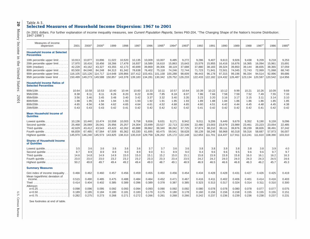
20

Mon

ey In

com

e in th

e Un

ited States: 2

00

1U

.S. Cen

sus Bu

reau

Table A-3.Selected Measures of Household Income Dispersion: 1967 to 2001(In 2001 dollars. For further explanation of income inequality measures, see Current Population Reports, Series P60-204, ‘‘The Changing Shape of the Nation’s Income Distribution:1947-1998’’)

Measures of incomedispersion 2001 20001 20002 1999 1998 1997 1996 19953 19944 19935 1992 1991 1990 1989 1988 19877 1986 19858

Household Income at SelectedPercentiles

10th percentile upper limit . . . . . . 10,913 10,877 10,896 11,022 10,520 10,135 10,009 10,007 9,485 9,272 9,286 9,407 9,613 9,926 9,438 9,209 9,218 9,25320th percentile upper limit . . . . . . 17,970 18,416 18,456 18,266 17,479 16,937 16,589 16,610 15,863 15,643 15,579 15,955 16,416 16,676 16,365 16,094 15,961 15,69150th (median) . . . . . . . . . . . . . . . 42,228 43,162 43,327 43,355 42,173 40,699 39,869 39,306 38,119 37,688 37,880 38,183 39,324 39,850 39,144 38,835 38,365 37,05980th percentile upper limit . . . . . . 83,500 84,048 84,248 84,313 81,342 78,638 76,402 75,118 74,246 72,744 71,723 71,941 72,501 74,045 72,743 72,069 71,068 68,74090th percentile upper limit . . . . . . 116,105 115,126 114,717 114,648 109,866 107,412 103,401 101,158 100,288 98,609 96,443 96,178 97,315 99,196 96,334 94,514 92,996 89,68695th percentile lower limit . . . . . . 150,499 149,273 149,588 150,857 143,378 139,183 134,281 130,342 129,752 126,233 122,433 122,182 124,432 126,487 123,134 120,597 120,542 114,956

Household Income Ratios ofSelected Percentiles

90th/10th . . . . . . . . . . . . . . . . . . . 10.64 10.58 10.53 10.40 10.44 10.60 10.33 10.11 10.57 10.64 10.39 10.22 10.12 9.99 10.21 10.26 10.09 9.6995th/20th . . . . . . . . . . . . . . . . . . . 8.38 8.11 8.11 8.26 8.20 8.22 8.09 7.85 8.18 8.07 7.86 7.66 7.58 7.59 7.52 7.49 7.55 7.3395th/50th . . . . . . . . . . . . . . . . . . . 3.56 3.46 3.45 3.48 3.40 3.42 3.37 3.32 3.40 3.35 3.23 3.20 3.16 3.17 3.15 3.11 3.14 3.1080th/50th . . . . . . . . . . . . . . . . . . . 1.98 1.95 1.94 1.94 1.93 1.93 1.92 1.91 1.95 1.93 1.89 1.88 1.84 1.86 1.86 1.86 1.85 1.8580th/20th . . . . . . . . . . . . . . . . . . . 4.65 4.56 4.56 4.62 4.65 4.64 4.61 4.52 4.68 4.65 4.60 4.51 4.42 4.44 4.45 4.48 4.45 4.3820th/50th . . . . . . . . . . . . . . . . . . . 0.43 0.43 0.43 0.42 0.41 0.42 0.42 0.42 0.42 0.42 0.41 0.42 0.42 0.42 0.42 0.41 0.42 0.42

Mean Household Income ofQuintiles

Lowest quintile. . . . . . . . . . . . . . . 10,136 10,440 10,474 10,558 10,003 9,758 9,656 9,631 9,171 8,942 9,011 9,206 9,449 9,679 9,352 9,190 9,159 9,096Second quintile . . . . . . . . . . . . . . 25,468 26,069 26,041 25,956 25,257 24,304 23,699 23,527 22,713 22,506 22,480 23,003 23,679 23,989 23,461 23,223 23,054 22,485Third quintile . . . . . . . . . . . . . . . . 42,629 43,412 43,543 43,422 42,262 40,888 39,862 39,340 38,262 37,725 37,874 38,210 39,111 39,876 39,239 38,826 38,491 37,242Fourth quintile . . . . . . . . . . . . . . . 66,839 67,485 67,564 67,509 65,362 63,330 61,695 60,475 59,541 58,628 58,139 58,248 58,968 60,318 59,316 58,687 57,973 56,007Highest quintile . . . . . . . . . . . . . . 145,970 146,240 145,573 143,825 138,313 135,019 129,758 126,202 125,172 122,148 112,653 111,701 114,437 117,911 113,241 111,610 108,390 103,310

Shares of Household Incomeof Quintiles

Lowest quintile. . . . . . . . . . . . . . . 3.5 3.6 3.6 3.6 3.6 3.6 3.7 3.7 3.6 3.6 3.8 3.8 3.9 3.8 3.8 3.8 3.9 4.0Second quintile . . . . . . . . . . . . . . 8.7 8.9 8.9 8.9 9.0 8.9 9.0 9.1 8.9 9.0 9.4 9.6 9.6 9.5 9.6 9.6 9.7 9.7Third quintile . . . . . . . . . . . . . . . . 14.6 14.8 14.9 14.9 15.0 15.0 15.1 15.2 15.0 15.1 15.8 15.9 15.9 15.8 16.0 16.1 16.2 16.3Fourth quintile . . . . . . . . . . . . . . . 23.0 23.0 23.0 23.2 23.2 23.2 23.3 23.3 23.4 23.5 24.2 24.2 24.0 24.0 24.3 24.3 24.5 24.6Highest quintile . . . . . . . . . . . . . . 50.2 49.8 49.7 49.4 49.2 49.4 49.0 48.7 49.1 48.9 46.9 46.5 46.6 46.8 46.3 46.2 45.7 45.3

Summary Measures

Gini index of income inequality . . 0.466 0.462 0.460 0.457 0.456 0.459 0.455 0.450 0.456 0.454 0.434 0.428 0.428 0.431 0.427 0.426 0.425 0.419Mean logarithmic deviation ofincome. . . . . . . . . . . . . . . . . . . . 0.515 0.490 0.485 0.475 0.488 0.484 0.464 0.452 0.471 0.467 0.416 0.411 0.402 0.406 0.401 0.414 0.416 0.403

Theil . . . . . . . . . . . . . . . . . . . . . . 0.414 0.404 0.402 0.385 0.389 0.396 0.389 0.378 0.387 0.385 0.323 0.313 0.317 0.324 0.314 0.311 0.310 0.300Atkinson:

e=0.25 . . . . . . . . . . . . . . . . . . . 0.098 0.096 0.095 0.092 0.093 0.094 0.093 0.090 0.092 0.092 0.080 0.078 0.078 0.080 0.078 0.077 0.077 0.075e=0.50 . . . . . . . . . . . . . . . . . . . 0.189 0.185 0.184 0.180 0.181 0.183 0.179 0.175 0.180 0.178 0.160 0.156 0.156 0.158 0.155 0.155 0.155 0.151e=0.75 . . . . . . . . . . . . . . . . . . . 0.282 0.275 0.273 0.268 0.271 0.272 0.266 0.261 0.268 0.266 0.242 0.237 0.236 0.239 0.236 0.238 0.237 0.231


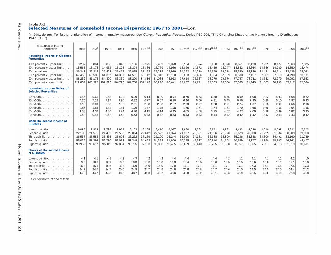
U.S. C

ensu

s Bureau

Mon

ey In

com

e in th

e Un

ited States: 2

00

1 2

1

Table A-3.Selected Measures of Household Income Dispersion: 1967 to 2001—Con(In 2001 dollars. For further explanation of income inequality measures, see Current Population Reports, Series P60-204. ‘‘The Changing Shape of the Nation’s Income Distribution:1947-1998’’)

Measures of incomedispersion 1984 19839 1982 1981 1980 197910 1978 1977 197611 197512 197412 13 1973 197214 197115 1970 1969 1968 196716

Household Income at SelectedPercentiles

10th percentile upper limit . . . . . . 9,237 8,864 8,888 9,040 9,156 9,275 9,439 9,028 8,924 8,874 9,128 9,070 8,651 8,120 7,999 8,177 7,963 7,32520th percentile upper limit . . . . . . 15,565 15,175 14,962 15,178 15,374 15,836 15,779 14,986 15,026 14,572 15,459 15,247 14,852 14,364 14,556 14,789 14,350 13,47450th (median) . . . . . . . . . . . . . . . 36,343 35,214 35,423 35,478 36,035 37,192 37,234 34,989 34,792 34,219 35,159 36,278 35,560 34,126 34,481 34,714 33,436 32,08180th percentile upper limit . . . . . . 67,450 65,585 64,397 64,357 64,501 65,742 65,315 62,130 60,863 59,436 61,084 62,069 60,508 57,457 57,881 57,519 54,790 53,18190th percentile upper limit . . . . . . 88,252 85,172 84,300 83,339 83,220 84,816 84,038 78,913 77,614 75,687 78,279 79,376 77,747 73,711 73,732 72,979 69,092 67,55395th percentile lower limit . . . . . . 112,832 108,920 107,312 104,720 104,788 107,243 105,226 100,441 97,037 94,771 97,609 98,388 97,399 91,243 91,505 90,209 85,717 85,334

Household Income Ratios ofSelected Percentiles

90th/10th . . . . . . . . . . . . . . . . . . . 9.55 9.61 9.48 9.22 9.09 9.14 8.90 8.74 8.70 8.53 8.58 8.75 8.99 9.08 9.22 8.93 8.68 9.2295th/20th . . . . . . . . . . . . . . . . . . . 7.25 7.18 7.17 6.90 6.82 6.77 6.67 6.70 6.46 6.50 6.31 6.45 6.56 6.35 6.29 6.10 5.97 6.3395th/50th . . . . . . . . . . . . . . . . . . . 3.10 3.09 3.03 2.95 2.91 2.88 2.83 2.87 2.79 2.77 2.78 2.71 2.74 2.67 2.65 2.60 2.56 2.6680th/50th . . . . . . . . . . . . . . . . . . . 1.86 1.86 1.82 1.81 1.79 1.77 1.75 1.78 1.75 1.74 1.74 1.71 1.70 1.68 1.68 1.66 1.64 1.6680th/20th . . . . . . . . . . . . . . . . . . . 4.33 4.32 4.30 4.24 4.20 4.15 4.14 4.15 4.05 4.08 3.95 4.07 4.07 4.00 3.98 3.89 3.82 3.9520th/50th . . . . . . . . . . . . . . . . . . . 0.43 0.43 0.42 0.43 0.43 0.43 0.42 0.43 0.43 0.43 0.44 0.42 0.42 0.42 0.42 0.43 0.43 0.42

Mean Household Income ofQuintiles

Lowest quintile. . . . . . . . . . . . . . . 9,089 8,833 8,786 8,995 9,122 9,295 9,410 9,057 8,990 8,798 9,141 8,863 8,493 8,036 8,010 8,098 7,911 7,303Second quintile . . . . . . . . . . . . . . 22,106 21,575 21,492 21,556 22,014 22,642 22,522 21,374 21,337 20,891 21,896 21,970 21,629 20,900 21,299 21,584 20,909 19,910Third quintile . . . . . . . . . . . . . . . . 36,557 35,584 35,465 35,603 36,232 37,269 37,100 35,244 35,000 34,181 35,188 35,899 35,296 33,888 34,300 34,491 33,160 31,789Fourth quintile . . . . . . . . . . . . . . . 55,036 53,393 52,730 53,033 53,349 54,662 54,328 51,606 50,795 49,637 50,810 51,608 50,669 48,177 48,350 48,307 46,261 44,477Highest quintile . . . . . . . . . . . . . . 99,955 96,617 95,119 92,894 93,705 97,133 95,880 90,465 88,639 86,443 88,735 91,528 90,967 85,365 85,607 84,913 81,019 80,601

Shares of Household Incomeof Quintiles

Lowest quintile. . . . . . . . . . . . . . . 4.1 4.1 4.1 4.2 4.3 4.2 4.3 4.4 4.4 4.4 4.4 4.2 4.1 4.1 4.1 4.1 4.2 4.0Second quintile . . . . . . . . . . . . . . 9.9 10.0 10.1 10.2 10.3 10.3 10.3 10.3 10.4 10.5 10.6 10.5 10.5 10.6 10.8 10.9 11.1 10.8Third quintile . . . . . . . . . . . . . . . . 16.4 16.5 16.6 16.8 16.9 16.9 16.9 17.0 17.1 17.1 17.1 17.1 17.1 17.3 17.4 17.5 17.5 17.3Fourth quintile . . . . . . . . . . . . . . . 24.7 24.7 24.7 25.0 24.9 24.7 24.8 24.8 24.8 24.8 24.7 24.6 24.5 24.5 24.5 24.5 24.4 24.2Highest quintile . . . . . . . . . . . . . . 44.9 44.7 44.5 43.8 43.7 44.0 43.7 43.6 43.3 43.2 43.1 43.6 43.9 43.5 43.3 43.0 42.8 43.8


22

Mon

ey In

com

e in th

e Un

ited States: 2

00

1U

.S. Cen

sus Bu

reau

Table A-3.Selected Measures of Household Income Dispersion: 1967 to 2001—Con(In 2001 dollars. For further explanation of income inequality measures, see Current Population Reports, Series P60-204. ‘‘The Changing Shape of the Nation’s Income Distribution:1947-1998’’)

Measures of incomedispersion 1984 19839 1982 1981 1980 197910 1978 1977 197611 197512 197412 13 1973 197214 197115 1970 1969 1968 196716

Summary Measures

Gini index of income inequality . . 0.415 0.414 0.412 0.406 0.403 0.404 0.402 0.402 0.398 0.397 0.395 0.397 0.401 0.396 0.394 0.391 0.388 0.399Mean logarithmic deviation ofincome. . . . . . . . . . . . . . . . . . . . 0.391 0.397 0.401 0.387 0.375 0.369 0.363 0.364 0.361 0.361 0.352 0.355 0.370 0.370 0.370 0.357 0.356 0.380

Theil . . . . . . . . . . . . . . . . . . . . . . 0.290 0.288 0.287 0.277 0.274 0.279 0.275 0.276 0.271 0.270 0.267 0.270 0.279 0.273 0.271 0.268 0.273 0.287Atkinson:

e=0.25 . . . . . . . . . . . . . . . . . . . 0.073 0.072 0.072 0.070 0.069 0.070 0.069 0.069 0.068 0.067 0.067 0.068 0.070 0.068 0.068 0.067 0.067 0.071e=0.50 . . . . . . . . . . . . . . . . . . . 0.147 0.147 0.146 0.141 0.140 0.141 0.139 0.139 0.137 0.136 0.134 0.136 0.140 0.138 0.138 0.135 0.135 0.143e=0.75 . . . . . . . . . . . . . . . . . . . 0.225 0.226 0.226 0.220 0.216 0.216 0.213 0.213 0.211 0.210 0.207 0.210 0.216 0.214 0.214 0.209 0.208 0.220

1Implementation of Census 2000-based population controls and a 28,000 household sample expansion.2 Reflects a correction to the March 2001 CPS weighting.3 Full implementation of 1990 census-based sample design and metropolitan definitions, 7,000 household sample reduction, and revised race edits.4 Introduction of 1990 census sample design.5 Data collection method changed from paper and pencil to computer-assisted interviewing. In addition, the March 1994 income supplement was revised to allow for the coding of different income amounts on

selected questionnaire items. Limits either increased or decreased in the following categories: earnings limits increased to $999,999; social security limits increased to $49,999; supplemental security income andpublic assistance limits increased to $24,999; veterans’ benefits limits increased to $99,999; child support and alimony limits decreased to $49,999.

6 Implementation of 1990 census population controls.7 Implementation of a new March CPS processing system.8 Recording of amounts for earnings from longest job increased to $299,999. Full implementation of 1980 census-based sample design.9 Implementation of Hispanic population weighting controls and introduction of 1980 census-based sample design.10 Implementation of 1980 census population controls. Questionnaire expanded to show 27 possible values from 51 possible sources of income.11 First year medians were derived using both Pareto and linear interpolation. Before this year all medians were derived using linear interpolation.12 Some of these estimates were derived using Pareto interpolation and may differ from published data which were derived using linear interpolation.13 Implementation of a new March CPS processing system. Questionnaire expanded to ask 11 income questions.14 Full implementation of 1970 census-based sample design.15 Introduction of 1970 census sample design and population controls.16 Implementation of a new March CPS processing system.



The 2001 Current PopulationSurvey (CPS) served as a tool fortesting a sample expansion of theAnnual Demographic Supplementand as a bridge to introduce newCensus 2000-based populationcontrols. The following sectiondiscusses the effects thesemethodological changes had onmeasures of income and earnings.

Sample Expansion

In 2001, the Census Bureau testeda 28,000 household expansion inthe sample for the CPS AnnualDemographic Supplement. Theoriginal sample size of approxi-mately 50,000 interviewed house-holds for the March 2001 CPS wasincreased to approximately78,000. The primary goal of thesample expansion was to producemore reliable state estimates of thenumber of low-income childrenwithout health insurance for theState Children’s Health InsuranceProgram (SCHIP) through reducedvariances. Although the SCHIPsample expansion was specificallytargeted toward producing betterchildren’s health insurance esti-mates at the state level, other stateestimates, as well as national esti-mates, improved. Further informa-tion about the SCHIP sampleexpansion is available on theinternet at: www.bls.census.gov/cps/ads/adsmain.htm.

Tables B-1 (at the national level)and B-2 (at the state level) presenttwo sets of data for 2000 to showthe effect of the sample expansion.One set of estimates is based onthe “Expanded” sample and theother set is based on the “Original”sample.

Effects of the SampleExpansion on NationalEstimates of Income

Nationally, median householdincome based on the expandedsample was not statistically differ-ent from the median derived fromthe original sample (see Table B-1).With few exceptions, medianincome did not change significant-ly for subgroups of the population.The exceptions, with lower medianincomes based on the expandedsample, are non-family householdswith a female householder, house-holds with a Black householder,and households in the Northeast.Households with a householderbetween the ages of 35 and 44years was the one demographicgroup in which the expanded sam-ple median income was higherthan the one derived from the orig-inal sample. The median earningsof women working full-time, year-round derived from the expandedsample was also higher. The percapita income of Blacks was lower,and the per capita income ofHispanics was higher, when basedon the expanded sample.

Effects of the SampleExpansion on State Estimatesof Household Income

Although no changes in state rank-ings were statistically significant,the sample expansion producedsignificantly different medianhousehold income estimates for 19states and the District of Columbia(see Table B-2). Ten states and theDistrict of Columbia had highermedian incomes, while nine stateshad lower median incomes. Theexpanded sample ranked Maryland

($54,717), although not statistical-ly different from Minnesota orAlaska, higher than the remaining47 states and the District ofColumbia. West Virginia ($29,526),although not statistically differentfrom Arkansas and Louisiana, wasranked lower than the remaining47 states and the District ofColumbia. In comparison, themedian income based on the origi-nal sample showed that Maryland($51,601) was not statistically dif-ferent from New Jersey, Minnesota,Alaska, Connecticut, Delaware,Virginia, New Hampshire,Colorado, or Hawaii, but wasranked higher than the remaining40 states and the District ofColumbia, while West Virginia($29,041) was not statistically dif-ferent from Arkansas andLouisiana, but was ranked lowerthan the remaining 47 and theDistrict of Columbia.

Introduction of Census 2000-Based Population Controls

The procedure used in developingestimates for the entire civiliannoninstitutional population for theCurrent Population Survey (CPS)involves the weighting of sampleresults to independent estimates ofthe population by sex, age, race,and Hispanic/non-Hispanic cate-gories. These independent esti-mates are developed by using civil-ian noninstitutional populationcounts from the decennial census-es and projecting them forward tocurrent years using data on births,deaths, and net migration.Beginning with the 2002 CPSAnnual Demographic Supplement,the independent estimates used as

Appendix B. SAMPLE EXPANSION AND INTRODUCTION OF CENSUS 2000-BASEDPOPULATION CONTROLS


control totals for the CPS are basedon civilian noninstitutional popula-tion benchmarks established byCensus 2000.

Table B-3 shows two sets of datafor 2000 to show the effect ofintroducing new population con-trols—one set using new Census2000-based population controlsand the other set using controlsbased on the 1990 census. Thefollowing is a brief discussion ofthe effects of the new populationcontrols on income.

With few exceptions, the use of newCensus 2000-based populationcontrols resulted in lower 2000

calendar year median householdincome estimates, although thedrops in income were all less than1.0 percent, median householdincome dropped for all regions inthe country, for households thatwere located inside and outsidemetropolitan areas, and for all racegroups. Use of the new controlsalso lowered the income of mosttypes of households and most ofthe age groups of householdersshown in Table B-3. Similar to theexperience of most households, theuse of the new Census 2000-basedpopulation controls lowered themedian earnings of full-time, year-round workers.

In contrast, use of the new Census2000-based controls raised themedian household income ofHispanics, family households main-tained by women with no husbandpresent, and those maintained byhouseholders 15 to 24 and 55 to 64years of age. The median incomeof households maintained by a manwith no wife present remained sta-tistically unchanged. The Census2000-based population controls alsoraised the per capita income ofmost population groups. Theexception was the per capitaincome of Blacks, which dropped by0.4 percent.


Table B-1.Comparison of 2000 Median Income Using the Expanded Sample and the Original Sampleby Selected Characteristics(Households and people as of March 2001)

Characteristics

Expanded sample Original sample Difference (expandedsample minus

original sample)

Percentchange in

medianincome

Number(thou-

sands)

Median income

Number(thou-

sands)

Median income

Value(dollars)



Value(dollars)



Populationcount(thou-

sands)

Medianincome

(dollars)

HOUSEHOLDSAll households . . . . . . . . . . . . . 106,289 42,105 219 106,418 42,151 324 –129 –46 –0.1

Type of HouseholdFamily households . . . . . . . . . . . . . 72,465 51,804 298 72,380 51,751 390 85 53 0.1

Married-couple families . . . . . . . 55,511 59,494 444 55,603 59,343 620 –92 151 0.3Female householder, no

husband present. . . . . . . . . . . . 12,754 28,237 507 12,525 28,126 650 229 111 0.4Male householder, no wife

present . . . . . . . . . . . . . . . . . . . . 4,200 42,166 847 4,252 42,143 1,360 –52 23 0.1Nonfamily households . . . . . . . . . . 33,823 25,466 273 34,039 25,439 378 –216 27 0.1

Female householder . . . . . . . . . 18,698 20,638 317 18,821 20,929 424 –123 *–291 *–1.4Male householder. . . . . . . . . . . . 15,126 31,553 352 15,218 31,269 526 –92 284 0.9

Race and Hispanic Origin ofHouseholder

All races2 . . . . . . . . . . . . . . . . . . . 106,289 42,105 217 106,418 42,151 324 –129 –46 –0.1White . . . . . . . . . . . . . . . . . . . . . . . . 88,604 44,166 321 88,543 44,232 452 61 –66 –0.1

Non-Hispanic White . . . . . . . . . . 79,419 45,833 303 79,375 45,910 433 44 –77 –0.2Black. . . . . . . . . . . . . . . . . . . . . . . . . 13,247 29,715 637 13,355 30,436 757 –108 *–721 *–2.4Asian and Pacific Islander . . . . . . 3,518 55,999 1,615 3,527 55,525 2,440 –9 474 0.9

Hispanic origin3. . . . . . . . . . . . . . . . 9,669 33,118 809 9,663 33,455 1,114 6 –337 –1.0

Age of Householder

Under 65 years . . . . . . . . . . . . . . . . 84,573 48,669 331 84,591 48,770 475 –18 –101 –0.215 to 24 years. . . . . . . . . . . . . . . 6,422 27,814 632 6,393 27,711 831 29 103 0.425 to 34 years. . . . . . . . . . . . . . . 18,604 44,533 704 18,554 44,477 1,020 50 56 0.135 to 44 years. . . . . . . . . . . . . . . 23,928 53,865 605 23,904 53,243 905 24 *622 *1.245 to 54 years. . . . . . . . . . . . . . . 21,681 57,667 735 21,797 58,217 1,278 –116 –550 –0.955 to 64 years. . . . . . . . . . . . . . . 13,939 44,776 732 13,944 44,993 1,002 –5 –217 –0.565 years and over . . . . . . . . . . . 21,716 23,118 291 21,827 23,047 423 –111 71 0.3

Region

Northeast . . . . . . . . . . . . . . . . . . . . . 20,237 43,940 714 20,212 45,118 923 25 *–1,178 *–2.6Midwest . . . . . . . . . . . . . . . . . . . . . . 24,539 44,396 553 24,496 44,647 814 43 –251 –0.6South . . . . . . . . . . . . . . . . . . . . . . . . 38,293 38,503 464 38,526 38,402 614 –233 101 0.3West . . . . . . . . . . . . . . . . . . . . . . . . . 23,220 45,103 630 23,185 44,759 834 35 344 0.8

Residence

Inside metropolitan areas . . . . . . . 85,786 44,848 331 85,737 44,986 447 49 –138 –0.3Outside metropolitan areas. . . . . . 20,503 33,046 679 20,681 32,844 796 –178 202 0.6

EARNINGS OF FULL-TIME,YEAR-ROUND WORKERS

Male . . . . . . . . . . . . . . . . . . . . . . . . . 58,588 37,355 166 58,734 37,339 225 –146 16 0.0Female . . . . . . . . . . . . . . . . . . . . . . . 41,198 27,479 179 41,571 27,352 178 –373 *127 *0.5

PER CAPITA INCOME

All races2 . . . . . . . . . . . . . . . . . . . 276,567 22,269 209 276,540 22,199 209 27 70 0.3White . . . . . . . . . . . . . . . . . . . . . . . . 226,360 23,515 242 226,401 23,415 242 –41 100 0.4

Non-Hispanic White . . . . . . . . . . 194,120 25,340 271 194,196 25,273 271 –76 67 0.3Black. . . . . . . . . . . . . . . . . . . . . . . . . 35,924 14,862 355 35,919 15,198 418 5 *–336 *–2.2Asian and Pacific Islander . . . . . . 11,535 22,948 1,216 11,332 22,457 1,230 203 491 2.2

Hispanic origin3. . . . . . . . . . . . . . . . 33,875 12,614 441 33,862 12,307 441 13 *307 *2.5

*Statistically significant change at the 90-percent confidence level.1For an explanation of confidence intervals, see ‘‘Standard errors and their use’’ at www.census.gov/hhes/income/income01/sa.pdf.2Data for American Indians and Alaska Natives are not shown separately in this table because of the small sample of those households.3People of Hispanic origin may be of any race.

Source: U.S. Census Bureau, Current Population Survey, 2001 Annual Demographic Survey.


Table B-2.Comparison of 2000 Median Income by State Using the Expanded Sampleand the Original Sample(Households as of March 2001)

States

Expanded sample Original sampleDifference (expanded

sample minusoriginal sample)

Percentchange in

medianincome

Numberof house-

holds (thou-sands)

Median income

Numberof house-

holds (thou-sands)

Median income

Numberof house-

holds (thou-sands)

Medianincome

(dollars)Value

(dollars)



Value(dollars)



United States. . . 106,289 42,105 219 106,418 42,151 324 –129 –46 –0.1

Alabama . . . . . . . . . . . 1,739 35,531 1,742 1,757 33,111 3,221 –18 *2,420 7.3Alaska . . . . . . . . . . . . . 225 53,152 1,926 224 50,767 2,685 1 *2,385 *4.7Arizona . . . . . . . . . . . . 1,832 39,825 2,038 1,848 41,454 2,208 –16 *–1,629 *–3.9Arkansas . . . . . . . . . . . 1,053 29,780 1,285 1,049 30,292 1,545 4 –512 –1.7California. . . . . . . . . . . 12,367 46,962 1,112 12,281 46,808 1,495 86 154 0.3Colorado . . . . . . . . . . . 1,639 48,403 2,114 1,660 48,548 2,820 –21 –145 –0.3Connecticut . . . . . . . . . 1,296 50,464 2,209 1,304 50,374 3,389 –8 90 0.2Delaware. . . . . . . . . . . 296 50,538 2,270 294 50,172 4,465 2 366 0.7District of Columbia . . 235 41,258 1,852 239 38,716 2,953 –4 *2,542 *6.6Florida . . . . . . . . . . . . 6,266 38,939 1,257 6,262 38,004 1,355 4 *935 *2.5

Georgia . . . . . . . . . . . 3,025 41,904 1,375 3,120 42,883 1,581 –95 *–979 *–2.3Hawaii . . . . . . . . . . . . . 402 51,296 1,956 408 48,096 3,399 –6 *3,200 *6.7Idaho . . . . . . . . . . . . . . 496 37,725 1,969 496 37,462 2,729 - 263 0.7Illinois . . . . . . . . . . . . . 4,568 46,136 1,612 4,521 46,435 1,953 47 –299 –0.6Indiana . . . . . . . . . . . . 2,347 40,952 1,655 2,360 39,636 2,773 –13 1,316 3.3Iowa. . . . . . . . . . . . . . . 1,132 41,168 1,346 1,126 42,949 2,311 6 *–1,781 *–4.1Kansas . . . . . . . . . . . . 1,048 41,220 1,911 1,061 37,858 3,364 –13 *3,362 *8.9Kentucky . . . . . . . . . . . 1,594 36,336 1,395 1,598 37,176 2,769 –4 –840 –2.3Louisiana. . . . . . . . . . . 1,685 30,763 1,367 1,696 30,230 2,139 –11 533 1.8Maine. . . . . . . . . . . . . . 529 37,504 1,405 509 41,659 1,984 20 *–4,155 *–10.0

Maryland . . . . . . . . . . . 2,093 54,717 2,213 2,065 51,601 3,320 28 *3,116 *6.0Massachusetts . . . . . . 2,463 47,103 2,295 2,431 46,982 2,823 32 121 0.3Michigan . . . . . . . . . . . 3,779 45,649 1,823 3,787 46,190 2,362 –8 –541 –1.2Minnesota . . . . . . . . . . 1,864 54,646 2,828 1,867 50,873 2,800 –3 *3,773 *7.4Mississippi. . . . . . . . . . 1,091 34,270 2,240 1,101 31,517 1,569 –10 *2,753 *8.7Missouri. . . . . . . . . . . . 2,151 45,165 1,944 2,144 47,471 3,019 7 *–2,306 *–4.9Montana . . . . . . . . . . . 357 32,958 1,670 363 32,046 2,055 –6 912 2.8Nebraska. . . . . . . . . . . 649 41,915 1,727 655 38,545 3,144 –6 *3,370 *8.7Nevada . . . . . . . . . . . . 704 45,888 1,762 713 44,737 2,362 –9 1,151 2.6New Hampshire . . . . . 484 51,133 2,058 492 48,904 3,909 –8 2,229 4.6New Jersey. . . . . . . . . 3,064 50,538 1,592 3,068 51,033 1,485 –4 –495 –1.0

New Mexico . . . . . . . . 660 35,136 2,066 670 35,252 3,200 –10 –116 –0.3New York. . . . . . . . . . . 7,089 40,838 975 7,070 41,597 1,426 19 *–759 *–1.8North Carolina . . . . . . 3,012 38,472 1,352 2,993 38,815 2,224 19 –343 –0.9North Dakota . . . . . . . 251 36,358 1,793 253 35,396 2,711 –2 962 2.7Ohio. . . . . . . . . . . . . . . 4,435 43,079 1,240 4,413 43,897 1,790 22 –818 –1.9Oklahoma . . . . . . . . . . 1,343 32,610 1,260 1,348 32,465 1,724 –5 145 0.4Oregon . . . . . . . . . . . . 1,353 42,631 1,576 1,363 42,463 2,719 –10 168 0.4Pennsylvania . . . . . . . 4,671 42,348 1,234 4,685 43,743 2,134 –14 *–1,395 *–3.2Rhode Island . . . . . . . 393 42,544 1,831 399 43,165 4,152 –6 –621 –1.4South Carolina . . . . . . 1,577 37,594 1,540 1,590 37,065 2,140 –13 529 1.4South Dakota . . . . . . . 290 36,682 1,165 293 36,162 2,114 –3 520 1.4

Tennessee. . . . . . . . . . 2,220 34,130 1,555 2,274 33,909 2,515 –54 221 0.7Texas . . . . . . . . . . . . . . 7,578 38,791 1,286 7,611 39,837 1,379 –33 *–1,046 *–2.6Utah. . . . . . . . . . . . . . . 705 47,649 1,749 718 45,261 2,074 –13 *2,388 *5.3Vermont. . . . . . . . . . . . 247 39,685 1,508 255 38,175 3,101 –8 1,510 4.0Virginia . . . . . . . . . . . . 2,740 47,189 1,757 2,774 50,032 3,693 –34 *–2,843 *–5.7Washington . . . . . . . . . 2,289 42,809 2,122 2,249 42,062 2,747 40 747 1.8West Virginia. . . . . . . . 746 29,526 1,084 755 29,041 1,235 –9 485 1.7Wisconsin . . . . . . . . . . 2,024 45,349 1,630 2,015 45,383 2,834 9 –34 –0.1Wyoming . . . . . . . . . . . 190 39,721 1,759 191 39,027 3,017 –1 694 1.8

- Represents zero or rounds to zero. * Statistically significant at the 90-percent confidence level.1For an explanation of confidence intervals, see ‘‘Standard errors and their use’’ at www.census.gov/hhes/income/income01/sa.pdf.



Table B-3.Comparison of 2000 Median Income Using Census 2000-Based Population Controls and1990 Census-Based Population Controls by Selected Characteristics(Households and people as of March 2001)

Characteristic

2000Census 2000-based controls

20001990 census-based controls

Difference (Census2000-based

controls minus1990 census-based

controls)

Percentchange in

medianincome

Number(thou-

sands)Value

(dollars)



Number(thou-

sands)Value

(dollars)



Number(thou-

sands)

Medianincome

(dollars)

HOUSEHOLDSAll households . . . . . . . . . . . . . . . . . . . . . 108,209 41,990 217 106,289 42,105 217 1,920 –115 *–0.3

Type of HouseholdFamily households . . . . . . . . . . . . . . . . . . . . 73,767 51,712 296 72,465 51,804 298 1,302 –92 *–0.2

Married-couple families . . . . . . . . . . . . . . 56,592 59,272 441 55,511 59,494 444 1,081 –222 *–0.4Female householder, no husband

present . . . . . . . . . . . . . . . . . . . . . . . . . . 12,900 28,264 502 12,754 28,237 507 146 27 *0.1Male householder, no wife present . . . . . 4,275 42,155 831 4,200 42,166 847 75 –11 -

Nonfamily households . . . . . . . . . . . . . . . . . 34,442 25,306 271 33,823 25,466 273 619 –160 *–0.6Female householder . . . . . . . . . . . . . . . . . 19,097 20,480 314 18,698 20,638 317 399 –158 *–0.8Male householder . . . . . . . . . . . . . . . . . . . 15,345 31,479 349 15,126 31,553 352 219 –74 *–0.2

Race and Hispanic Origin ofHouseholder

All races 2 . . . . . . . . . . . . . . . . . . . . . . . . . 108,209 41,990 217 106,289 42,105 217 1,920 –115 *–0.3White. . . . . . . . . . . . . . . . . . . . . . . . . . . . . . . 90,030 43,916 319 88,604 44,166 321 1,426 –250 *–0.6

Non-Hispanic White . . . . . . . . . . . . . . . . . 80,527 45,623 301 79,419 45,833 303 1,108 –210 *–0.5Black . . . . . . . . . . . . . . . . . . . . . . . . . . . . . . . 13,174 29,667 646 13,247 29,715 637 –73 –48 *–0.2Asian and Pacific Islander . . . . . . . . . . . . . . 3,963 55,757 1,564 3,518 55,999 1,615 445 –242 *–0.4

Hispanic origin 3 . . . . . . . . . . . . . . . . . . . . . . 10,034 33,168 786 9,669 33,118 773 365 50 *0.2

Age of HouseholderUnder 65 years. . . . . . . . . . . . . . . . . . . . . . . 85,740 48,633 329 84,573 48,669 331 1,167 –36 *–0.1

15 to 24 years. . . . . . . . . . . . . . . . . . . . . . 6,409 27,847 638 6,422 27,814 632 –13 33 *0.125 to 34 years. . . . . . . . . . . . . . . . . . . . . . 19,031 44,414 693 18,604 44,533 704 427 –119 *–0.335 to 44 years. . . . . . . . . . . . . . . . . . . . . . 24,054 53,762 602 23,928 53,865 605 126 –103 *–0.245 to 54 years. . . . . . . . . . . . . . . . . . . . . . 21,969 57,642 727 21,681 57,667 735 288 –25 -55 to 64 years. . . . . . . . . . . . . . . . . . . . . . 14,277 44,853 722 13,939 44,776 732 338 77 *0.265 years and over. . . . . . . . . . . . . . . . . . . 22,469 23,083 286 21,716 23,118 291 753 –35 *–0.2

RegionNortheast . . . . . . . . . . . . . . . . . . . . . . . . . . . 21,022 43,750 701 20,237 43,940 714 785 –190 *–0.4Midwest. . . . . . . . . . . . . . . . . . . . . . . . . . . . . 25,222 44,261 544 24,539 44,396 553 683 –135 *–0.3South . . . . . . . . . . . . . . . . . . . . . . . . . . . . . . 38,852 38,389 461 38,293 38,503 464 559 –114 *–0.3West . . . . . . . . . . . . . . . . . . . . . . . . . . . . . . . 23,113 44,915 648 23,220 45,103 630 –107 –188 *–0.4

ResidenceInside metropolitan areas. . . . . . . . . . . . . . . 87,276 44,695 332 85,786 44,848 331 1,490 –153 *–0.3Outside metropolitan areas . . . . . . . . . . . . . 20,933 32,913 673 20,503 33,046 679 430 –133 *–0.4

EARNINGS OF FULL-TIME,YEAR-ROUND WORKERSMale . . . . . . . . . . . . . . . . . . . . . . . . . . . . . . . 59,602 37,252 166 58,588 37,355 166 1,014 –103 *–0.3Female . . . . . . . . . . . . . . . . . . . . . . . . . . . . . 41,719 27,462 168 41,198 27,479 179 521 –17 *–0.1

PER CAPITA INCOMEAll races 2 . . . . . . . . . . . . . . . . . . . . . . . . . 279,517 22,346 188 276,567 22,269 209 2,950 77 *0.3

White. . . . . . . . . . . . . . . . . . . . . . . . . . . . . . . 228,208 23,582 224 226,360 23,515 242 1,848 67 *0.3Non-Hispanic White . . . . . . . . . . . . . . . . . 193,931 25,529 258 194,120 25,340 271 –189 189 *0.7

Black . . . . . . . . . . . . . . . . . . . . . . . . . . . . . . . 35,597 14,796 339 35,924 14,862 355 –327 –66 *–0.4Asian and Pacific Islander . . . . . . . . . . . . . . 12,693 23,350 1,115 11,535 22,948 1,216 1,158 402 *1.8

Hispanic origin 3 . . . . . . . . . . . . . . . . . . . . . . 36,093 12,651 392 33,875 12,614 441 2,218 37 *0.3

- Represents zero or rounds to zero. *Statistically significant change at the 90-percent confidence level.1For an explanation of confidence intervals, see ‘‘Standard errors and their use’’ at www.census.gov/hhes/income/income01/sa.pdf.2Data for American Indians and Alaska Natives are not shown separately in this table because of the small sample of those households.3Hispanics may be of any race.


Money Income in the United States: 2001 - Census.gov Income in the United States: 2001 Demographic...

Documents

Transcript of Money Income in the United States: 2001 - Census.gov Income in the United States: 2001 Demographic...