First draft: September 2002

Revised: February 2003

Please do not quote without permission

Money in a Theory of Banking

Douglas W. Diamond Raghuram G. Rajan

University of Chicago University of Chicago

and NBER and NBER

Abstract

We explore the connection between money, banks, and aggregate credit by introducing money in a simple “real” model of banking. Because of the nature of their business, banks are susceptible to aggregate shortages of consumption goods. We find that under very special circumstances, banks can insure themselves against these destructive shortages by issuing nominal deposits (i.e., denominated in money) instead of real deposits. In general, however, banks will not be completely insured. In fact, by issuing nominal demand deposits, banks leave themselves exposed to significant increases in their real repayment burden if there is a shortfall of money. This could exacerbate shortages and lead to a severe contraction in credit. Our analysis makes transparent how changes in the supply of money can work through banks to affect real economic activity. It also suggests how bank failures could lead to a fall in prices and a contagion of bank failures, as described by Friedman and Schwartz (1963).

We are grateful for financial support from the National Science Foundation and the Center for Research on Security Prices. Rajan also thanks the Center for the Study of the State and the Economy for financial support. We thank John Cochrane, Jeff Lacker and Jeremy Stein for helpful conversations on this topic.

1

What is the connection between money, banks, and aggregate credit? When can

expansionary monetary policy lead to expanded bank credit? And when can expansionary

monetary policy help avert bank failures? These are the questions that motivate this paper.

In our earlier work, we built a “real” model of a bank. We showed in Diamond and Rajan

(2001) that a bank financed with demand deposits is an efficient institution to channel resources

from investors who have uncertain consumption needs to firms that are hard to collect from.

Essentially, the bank acquires skills to force the borrowing firm to repay, and commits to use

these skills on behalf of investors by issuing demandable claims. So long as there is no aggregate

shortage of goods, this structure also allows banks to meet the uncertain investor demand for

goods. Thus a bank may be well suited to play a central role in funding potentially long term

projects while allowing investors to consume when needed.

Unfortunately, the very institutional feature – demandable claims – that allows the bank

to perform its essential functions also exposes the banking system to the risk that there might be a

mismatch between the production of consumption goods and the immediate consumption needs

of depositors. Even if the mismatch is merely due to delay in production and not because of any

impairment of the long-term production possibilities of the economy, we show in Diamond and

Rajan (2002a) that such an aggregate shortage of consumption goods (also termed a real

“liquidity shortage”) can be amplified by the banking system. If a bank cannot attract sufficient

consumption goods relative to its non-renegotiable depositor claims, it will be run. This can occur

even if depositors have the most optimistic beliefs possible about the system, and it could lead to

the termination of projects, bank failures, and sometimes even a contagious meltdown of the

entire banking system. In short, the features that make a bank such an effective institution in the

normal course also make the banking system amplify seemingly benign shortfalls in the supply of

consumption goods.

We derived all this in an economy where all contracts paid in goods, and there was no

money. Yet bank deposits and loans repay money, not goods, and banks hold a substantial

2

amount of money and bonds on their balance sheets. What would happen if we introduced money

and bonds in this model, and allowed for deposit contracts denominated and repayable in money

(i.e., nominal deposits)? Would the systemic problems we have documented vanish? Can

monetary policy play any useful role? How would it work? It is to these important questions that

we turn in this paper.

Money has two roles in our model. First, it is a claim on the government and therefore

can be used to pay taxes. Call this the fiscal demand for cash. Second, it is necessary for buying

cash goods as in the cash-in-advance literature (see Clower [1967] and Lucas-Stokey [1987]).

These could be goods that are illegal like drugs, goods such as services that are sold in

transactions where the seller may seek to keep his identity hidden from tax authorities, or just

goods encountered serendipitously where the relative cost of establishing a credit transaction may

be too high. Call this the transactions demand for cash. Which demand predominates is important

in what follows.

Suppose now that banks issue deposits whose repayment is denominated in money.

Suppose further that the value of money is determined primarily by its fiscal demand – its value

in paying taxes (we will indicate later when this will be the case). We consider taxes only on

production. Since the present value of taxes will be proportional to the present value of

production, the value of money will be low -- that is, prices will be high for a given level of

money -- when the present value of production is low. A delay in production (resulting in a

temporary potential shortage of consumption goods) will result in a low present value of

production, a low value of money, and thus a low real repayment obligation on deposits when

deposits are denominated in money. Thus, under certain circumstances, banks can hedge against

shortfalls in aggregate real liquidity by issuing nominal deposits.

But what if the transactions demand for cash is significant? To the extent that cash

transactions are driven by other factors than aggregate economic activity, the real repayment

3

obligation on nominal deposits may not fall with delays or declines in aggregate production.

What is more problematic for banks is that when they issue nominal demandable deposits, they

are left particularly exposed to fluctuations in the purchasing power of money: Since depositors

can withdraw money on demand, in a period when cash transactions are very lucrative (for

example, because the supply of money is low relative to available cash goods) banks will be

forced to push up the interest rates offered on demandable deposits significantly so as to keep all

depositors from withdrawing. In turn, this will increase the real repayment obligations of the

banks, potentially without limit. Nominal deposit contracts may not just fail to protect banks from

fluctuations in aggregate real liquidity, they will also leave banks exposed to fluctuations in

monetary conditions.

Our analysis then suggests a channel through which monetary policy can affect credit

and thus aggregate economic activity. By increasing the money supply available for transactions

when the transactions demand is high (and by committing to provide monetary support in the

future when needed), the monetary authority keeps the price level stable, thus limiting depositor

incentives to withdraw, and consequently limiting both nominal interest rates and future real

repayment obligations of banks. Banks then will respond by continuing, rather than curtailing,

credit to long-term projects, thus enhancing aggregate economic activity.

Our view of the monetary transmission mechanism could then be termed a version of the

bank lending channel view (see Bernanke and Gertler (1995) or Kashyap and Stein (1997)) for

comprehensive surveys) but with an important difference. According to the traditional lending

channel view, monetary policy affects bank loan supply, which in turn has an independent and

significant effect on aggregate economic activity (this does not exclude any effects of movements

in the interest rate or changes in the quality of corporate balance sheets). Three assumptions have

been thought to be key to the centrality of banks in the transmission process: (i) binding reserve

requirements tie the issuance of bank demand deposits to the availability of reserves (ii) banks

cannot substitute between demand deposits and other forms of finance easily so they have to cut

4

down on lending when the central bank curtails reserves (iii) client firms cannot substitute

between bank loans and other forms of finance, so they have to cut down on economic activity.

The concern with the traditional view of the bank lending channel is that as reserve

requirements have been eliminated for almost all bank liabilities except demand deposits, the

argument that banks will find it difficult or expensive to raise alternative forms of financing to

demand deposits becomes less persuasive (see, for example, the critique by Romer and Romer

(1990)). But there does seem to be strong evidence that monetary policy has effects on bank loan

supply (Kashyap, Stein, and Wilcox (1995), Ludvigson (1996)), has greater effect on banks at

times when their balance sheets look worse (Gibson (1996) and has the greatest effect on the

policies of the smallest and least credit worthy banks (Kashyap and Stein (2000)).

In contrast to traditional models of the lending channel, our model does not rely on

reserve requirements. An increase in the money supply increases financial liquidity, which

alleviates the real liquidity demands on banks, which then allows them to fund more long-term

projects to fruition. Thus it is perhaps best to term ours the liquidity channel of transmission.

Finally, we turn in the paper from the mechanism of transmission of monetary policy to

examine the possibility of financial contagion. As we have seen, a shortage of money depresses

the price of cash goods making it very attractive for bank depositors to withdraw money to buy

them. The resulting spike in nominal interest rates banks have to pay can make the banks

insolvent, precipitating runs or significantly curtailing lending. If depositors who run want only

cash (i.e., they are not willing to accept deposits elsewhere in the banking system perhaps because

they need time to search for a high quality bank), run banks have to sell all their assets for cash.

This increases the volume of cash transactions, even while the money stock does not change,

further depressing the price of cash goods. Purchases using cash become even more lucrative for

those who can withdraw it, further increasing the rate healthy banks have to pay to keep their

depositors in. Even otherwise healthy banks could now fail. Thus the kind of contagion described

in Friedman and Schwartz (1963) can take place in our model if there is a shortage of money.

5

The rest of the paper is as follows. In section I, we describe the framework, in section II

we describe the problems with real deposit contracts and the circumstances under which nominal

contracts can improve upon them. In section III, we examine how monetary policy is transmitted

in our model and how contagion can take place, and then we conclude.

I. The Framework

1.1. Agents, Preferences, Endowments, Technology.

We will first lay out the simple “real” model then overlay it with a role for money.

Consider an economy with three types of risk neutral agents: investors, entrepreneurs, and

bankers and three dates: 0, 2, and 4 (the intervening dates are introduced later). Investors get

utility only from near-term consumption, that is, their utility is the sum of consumption before

date 2. All other agents get equal utility from long-term consumption also, so their utility is the

sum of consumptions at all dates including date 4.

Investors are each endowed initially with a fraction of a unit of good. No other agent is

endowed with goods. Goods can be stored at a gross real return of 1. They can also be invested in

projects.

Each entrepreneur has a project, which requires the investment of a unit of good before

date 0. It pays off C produced goods at date 2 if the project produces early or C at date 4 if the

project is delayed and produces late. There is a shortage of endowments of goods initially relative

to projects that can be invested in.

1.2. Projects and the non-transferability of skills The primary friction in the model is that those with specific skills will earn a rent from

future surplus produced because they cannot commit to using their human capital on behalf of

others. This implies that they will not be able to borrow the full value of the surplus they can

produce with an asset or sell the asset for the amount they can produce with it. Both projects and

loans to projects will thus be illiquid because of the inalienability of human capital (see, Hart and

Moore (1994)).

6

Since entrepreneurs have no endowments, they need to borrow to invest. Each

entrepreneur has access to a banker who has, or can acquire during the course of lending,

knowledge about an alternative, but less effective, way to run the project. The banker’s specific

knowledge allows him to (make the credible threats that will enable him to) collect γC from an

entrepreneur whose project just matures.1 No one else has the knowledge to collect from the

entrepreneur.

Regardless of whether a project is early or late, the banker can also restructure the project

at any time to yield c in date-2 goods – intuitively, restructuring implies stopping half finished

projects and salvaging all possible produced goods from them. Restructured projects can be

collected by anyone. We assume

1c C Cγ< < < , (1.1)

Since no one other than the bank has the specific skills to collect from the entrepreneur, the loan

to the entrepreneur is illiquid in that the banker will get less than γC if he has to sell the loan

before the project matures. Any buyer will realize that the banker will extract a future rent for

collecting the loan, and the buyer will reduce the price he pays for the loan accordingly. In fact,

bank loans are so dependent on the banker’s specific skills for collection (that is, they are so

illiquid) that the banker prefers restructuring projects to selling them.

Since there is a shortage of endowment relative to projects, only a select few

entrepreneurs get a loan from their respective banks to buy a unit of the good from investors.

Entrepreneurs will have to promise to repay the maximum possible, γC, to obtain the loan.

1.3. Financing Banks

We analyze the general equilibrium effects in an economy where banks finance the

illiquid loans with both demand deposits and bank capital. Our positive results do not depend on

the reason that this form of finance is used. Our previous work has argued that these contracts

1 See Diamond and Rajan (2001a) for an extensive form game with this outcome. The problem with committing human capital that they model appears first in Hart and Moore (1994).

7

serve to allow the bankers to commit to collect the loans on behalf of outsides. It is useful to

briefly recount the reasons here.

Bankers themselves have no endowment, so they have to persuade investors to entrust

them with their money. But ordinary investors, unlike the banker, cannot collect from the

entrepreneur. The problem then is that having obtained investors’ money promising a certain

repayment, the banker can threaten to hold back his collection skills unless investors reduce the

required repayment. Since even if courts can enforce financial contracts they cannot compel the

banker to contribute his human capital, investors will be prey to attempts at strategic

renegotiation by the banker. The prospect of having the promised repayment renegotiated down

would seriously impair the amount investors are willing to entrust the banker with. Therefore, the

banker has to find a way to commit to using his skills on behalf of investors, else he will not be

able to raise enough to finance the loan he has made .

The way for the banker to finance lending while committing his human capital to the

service of investors is to issue uninsured demand deposits. Because of the "first come, first

served" aspect of uninsured demand deposits, they cannot be negotiated down. This is because

depositors are liable to run to demand repayment if they ever apprehend that they will be paid less

than their due (even though this hurts depositors collectively), thus destroying the banker’s rents

(see Diamond-Rajan (2001) for details). Thus if a banker has promised to pay depositors dt, they

want to consume at date t, and the banker has enough resources at that date, he will make the

payment.2

But while the collective action problem inherent in demand deposits enables the banker

to commit to repay if he can (that is, avoid strategic defaults), it exposes the bank to destructive

runs if he truly cannot pay (it makes non-strategic default more costly): when depositors demand

repayment before projects have matured and the bank does not have the means of payment, it will

2 For other models where runs or short term debt serve as a source of discipline, see Calomiris and Kahn (1991) and Jeanne (2000). The difference in Diamond-Rajan (2001) is that the run is particularly useful in disciplining an intermediary, even if it is not effective in disciplining a corporation that borrows directly.

8

be forced to restructure projects to get c immediately instead of allowing them to mature and

generate γC.

To mitigate the latter problem, the bank can also issue some capital (long term bonds or

equity) as buffer. The advantage of capital is that payments to it adjust to the residual value of the

bank – specifically, Diamond and Rajan (2000) present an extensive form game where if the

value of bank assets is v at date t, capital gets 2

tv d−. If there is uncertainty about bank asset

values, the bank can avoid destructive runs if it raises some money via capital in lieu of deposits.

The disadvantage is that the banker, unlike with deposits, will absorb the remaining residual

amount of 2

tv d−as rents. Our focus here is not on the ex ante optimal capital structure for the

bank. So we will assume that the un-modeled uncertainty facing a bank on its loans, or an explicit

capital requirement, requires it to finance at least fraction k≥0 of the loans it carries on the books

with capital. This will imply, for example, that for every late project the bank finances at date 2, it

can promise to pay out to depositors and capital only

(1 )Ck

γ+

(1.2)

at date 4, with the rest (= (1 )k C

kγ+

) absorbed by the banker as rent at date 4.3 The key results are

qualitatively unchanged if we do not require that the bank issue capital. We add bank capital to

the model only to understand its effects.

3 From the definition, we have

12 4

12 4

( )

( )

C dk

C d

γ

γ

−=

+ where the numerator on the right hand side is the date-4

value of capital (per late project), and the denominator is the value of capital plus date-4 maturing deposits. Therefore, the total amount that can be pledged to investors at date 2 out of the amount the bank collects

from late entrepreneurs at date 4 is the denominator, which on substituting for d4, works out to 1

C

k

γ

+.

9

Each bank faces an identical pool of entrepreneurs before date 0. But at date 0, the

fraction of the funded projects that turn out to be early could differ. A bank’s projects could all

turn out to be early (type G bank) or only a fraction αB < 1 could be early (type B bank). The

fraction of banks of type G in state s is ,G sθ and the fraction of early projects for the B type bank

is ,B sα . In what follows, we will suppress the dependence on the state for notational convenience.

All quantities will henceforth be normalized by the total initial endowment of goods.

1.4. Timing.

Before date 0. Investors are endowed with goods, invest them in competitive banks in return for

bank claims (deposits and capital) that make them better off in expectation than storage. Each

bank offers to repay d0 on demand per unit of good they get from investors and a commensurate

value on capital. Banks lend the goods to entrepreneurs in return for a promise to repay γC on

demand. Entrepreneurs invest the goods in projects.

Date 0. Uncertainty is resolved: everyone learns which entrepreneurs’ projects are early and

which are late, and thus what fraction αi of a bank i’s projects are early. If depositors anticipate

that, given the realized state of nature, the bank will not be able to pay them at date 2 an amount

that weakly dominates the consumption they obtain by withdrawing immediately, they will run

immediately. This will force the bank to first pay out all the goods it has, and then restructure

projects to generate the goods needed to pay depositors. If no run occurs, the bank decides how

to deal with each late project – whether to restructure it if proceeds are needed before date 4, or

perhaps get greater long run value by rescheduling the loan payment from date 2 to date 4 and

keeping the project as a going concern.

Date 2. Entrepreneurs with early projects will produce C, and repay the bank γC. This leaves

them with (1-γ)C to invest as they will. The bank obtains repayments from early entrepreneurs,

proceeds from restructured late projects, and new investments by early entrepreneurs and other

bankers with surplus. It must meet its capital requirement on this date (if one is imposed). It uses

10

these to repay date-0 investors. Investors present their claims and are paid goods, which they

consume.

Date 4. Late entrepreneurs repay banks and banks repay date-2 investors (early entrepreneurs

and other bankers). Entrepreneurs and bankers consume.

II. Aggregate Liquidity Shortages and Bank Credit.

We showed in Diamond and Rajan (2001) that banks and their fragile liability structures

are essential to facilitate the flow of credit from investors with uncertain consumption needs to

entrepreneurs who have hard-to-pledge cash flows. If investors lent directly, acquired collection

skills, but wanted to consume at an interim date, they would have to sell their loans at a huge

discount. Far better to hold demand deposits on a bank and let the bank acquire the collection

skills. If the investor wants to consume at an interim date, the bank will pay him and refinance by

borrowing from others (early entrepreneurs) who have a surplus. In this way, the bank does not

interrupt the late, but valuable, project while also allowing the investor to consume a larger

amount when he desires consumption.

Unfortunately, the liability structure of banks leaves them exposed to temporary aggregate

shortages of goods. A small delay in the supply of goods relative to their demand can propagate

through bank credit contraction and bank failures into a longer term, and more widespread

adverse shock to production. This is what we show now.

2.1. Banks’ maximization problem

Because the G type banker’s projects all mature at date 2, he will have enough to repay

investors provided 0C dγ ≥ . Let the gross real interest rate between date i and date j, rij . Now r02

is 1 because everyone is indifferent between consumption at date 0 and at date 2 and no real

investments between those dates offer a higher return.

11

If the B bank is expected to survive, the B-type banker, who takes prices and interest

rates as given, has the following, more complicated, decision problem: What fraction of late

projects does he restructure at date 0 so as to maximize his consumption while constrained by the

necessity to pay off all bank claimants?

The objective function is very simple. The banker consumes the residual claim after

paying off claimants on the bank. Given prices and interest rates, there is a particular level of

restructuring that maximizes the value received by initial outside claimants on the bank. This is

what they will demand regardless of the actual level of restructuring the banker undertakes.

Because he holds the residual claim, and because the value of outside claims are invariant to the

level of restructuring, the banker will choose the level of restructuring to maximize the

discounted consumption produced by the bank’s assets, constrained by the requirement that bank

claimants have to be paid.

We start by determining how much the bank can pay out at date 2. Its resources are the

repayment collected on early loans, and the amount it can raise by restructuring or borrowing

against late loans (this will differ from the discounted consumption the bank’s assets will produce

because the bank cannot raise money against its prospective rents).4 Let the banker of type i

restructure µi of his late projects (since all of a G type banker’s projects are early, µG=0). Then

the value he can raise in date-2 consumption goods is

2424

( , ) (1 ) (1 )(1 )(1 )

i i i i i i i Cv r C c

k rγ

µ α γ µ α µ α= + − + − −+

(2.1)

The first term is the amount repaid by the α early entrepreneurs whose projects mature at date 2.

The second term is the amount obtained by restructuring late projects. The third term is the

amount the bank can raise (in new deposits and capital – see (1.2)) against late projects that are

4 We show in Diamond and Rajan (2003) that the bank will not store any goods.

12

allowed to continue without interruption till date 4, where r24 is the real interest rate banks offer

on deposits between dates 2 and 4 (this need not be 1 because the initial investors do have a

preference for date 2 consumption over date 4 consumption).

The total amount depositors and bank capital will have to be paid is '

'24 0( , )max

2

iv r dµ

µ +

.5 The

B type banker’s problem is then

124

(1 ) (1 )(1 )maxB

B B B B B CC c

rµ

γα γ µ α µ α+ − + − − (2.2)

s.t. '

'24 0

24

( , )

( , )max

2

B

B B

v r d

v r µ

µ

µ

+

≥ (2.3)

The solution to this problem can be easily characterized.

Lemma 1: Let (1 )

Ck c

R γ+

= and C

Rc

γ= . If r24 <R, the banker will not restructure any projects

(so that µB=0) and the bank will survive provided it can pay date-0 depositors – provided

24 0(0, )Bv r d≥ .6 If 24R r R< < , the banker will restructure the minimum fraction µB such that

24 024

( , )( , )

12

BB B v r d

v rµ+

≥ . Finally, if 24r R≥ , the banker will restructure all late projects and

the bank will survive provided 24 0(1, )Bv r d≥ .

5 Capital gets (v-d)/2 while depositors get d. Also, v is the value of the assets to outsiders in their best use,

that is, with 'µ set at the value that maximizes v. 6 This condition also ensures the bank will pay off capital.

13

The lemma indicates the fraction the banker restructures increases with the real interest

rate. At low interest rates (r24 <R), the banker gets more value and can raise more by continuing

late projects. At high interest ( 24r R≥ ) the banker gets more value and can raise more by

restructuring late projects. But at intermediate rates, the banker has an incentive to continue,

though he can pay claimants more by restructuring. This is because the banker gets rents from

continued late projects that bank claimants do not see (the last term in (2.2) is greater than the last

term in (2.1)). So he will restructure the minimum that will be necessary to pay off claimants.

Other decisions are less complicated. The entrepreneur’s production decision is entirely

passive – he produces in due course if his project is not restructured by the bank beforehand. If he

produces, he repays the bank. Early entrepreneurs invest their residual goods (of (1 )Cγ− ) in the

bank at date 2 if it can credibly promise to repay r24 ≥ 1.

2.2. Equilibrium Condition and aggregate credit.

The only price at date 2 in this “real” model that can adjust in response to a shortage of

date 2 goods is the relative price of date 4 to date 2 consumption: the real interest rate, r24. Since

investors can express their purchasing power only with their claims on the bank, the demand for

consumption (real liquidity) is the total real value of their claims on the bank. The real interest

rate ensures the total investor demand for goods at date 2 is weakly less than the supply of goods.

( )24 0 24 0

' '( ', ) ( ', )

(1 (1 ) (1 )2 2

max max )

G B

G G G G B B B

v r d v r dcC Cµ µ

µ µθ θ θ θ α α µ

+ ++ − + − + −≤

(2.4)

The real side of our model should now be fairly clear. The adverse shocks in our model

are merely delays in the timing of production – adverse shocks to the quantities produced would

only exacerbate the problems. Even though the total production possibilities of the economy over

14

dates 2 and 4 do not change with increases in the fraction of B banks, (1- θ ), and the fraction of

their late projects, (1- Bα ), the amount of consumption goods available at date 2 (aggregate real

liquidity) falls. Given prices, both supply and demand for liquidity adjust with the real interest

rate. Supply rises as banks restructure more late projects. The fraction of late projects a B type

bank continues, 1 Bµ− , could be thought of as a measure of the credit it extends, so credit falls.

Demand falls as a higher real interest rate reduces the real value of the B type bank’s capital, and

thus reduces the purchasing power initial investors have. Hence an incipient liquidity shortage is

alleviated by an increase in the real rate, which increases the supply (and reduces credit) while

reducing the demand for liquidity.

Let the total supply of consumption goods not be enough to meet the total demand

without some restructuring by B type banks. If the system is in a unique equilibrium where both

types of banks survive and the B type banks restructure a positive fraction of their late projects,

we have

Proposition 1: For a given level of deposits issued at date –1,

(i) Equilibrium credit extended at date 2, (1 )Bµ− , increases with an increase in the

fraction of G type banks, .Gθ

(ii) Equilibrium credit extended at date 2, (1 )Bµ− , increases with the fraction of

projects of B type banks that are early, Bα .

(iii) For every Gθ , there is an *α (possibly 0) such that B type banks are insolvent iff

*Bα α< .

Proof: See appendix.

The availability of consumption goods (absent restructuring) at date 2 increases in both Gθ and

Bα . The proposition indicates that when the bank issues real deposits, aggregate bank credit

increases with this availability. A mere delay in production with no reduction in potential total

15

output can cause banks to tighten credit, and even fail. Of course, if late projects were not just late

but also produced less than C, matters could be much worse. The bottom-line is that banks make

it possible for investors to consume on demand even while funding long term illiquid projects.

But this leaves them exposed to aggregate shortages of consumption relative to demand.

Production delays force banks to squeeze liquidity out of their loans. Since these fetch little value

in a sale, banks will be forced to restructure the underlying projects, thereby curtailing production

and credit. If severe enough, aggregate delays can also cause banks to fail.

2.3. Bank failures.

Recall that if a bank is expected to fail, depositors run and demand payment immediately.

Since projects pay at date 2 at the earliest, and since the bank obtains more from restructuring

rather than selling the illiquid project loans, depositors in a run bank get the restructured value of

the bank’s loans. The run bank’s excess demand for liquidity collapses to zero, thus potentially

contributing towards restoring equilibrium between demand and supply. 7 However, failure is

inefficient because early projects could have produced C in a timely manner to satisfy the

consumption needs of date-0 investors, but now produce only c.

In other words, if the supply of real liquidity is low, a shortage may persist even after

banks curtail credit and restructure projects, and there may be no way to bridge the gap without

banks failing. The collective action problem inherent in demand deposits is now destructive for it

forces the costly production of consumption goods when none is really needed.

When all contracts are real, there is only one price – the real interest rate – which can

adjust to clear markets. The system may have insufficient degrees of freedom to adjust to an

adverse shock, resulting in the stark consequences we have documented. Could the introduction

of other assets including financial assets serve to mitigate this? Would the fact that real world

7 Though see Diamond and Rajan (2002a) where a bank failure can spread because a bank failure increases the excess demand for liquidity.

16

banks pay out cash rather than goods change things? We now introduce a role for money, then

determine prices in this economy, and finally see whether aggregate shortages still persist, honing

in on the link between money, banking, and real economic activity.

III. Money and Banking

We focus on two natural sources of value for money. First, money (and any maturing

government liability) can be used to pay taxes. This is one anchor for the value of money, which

we shall term the fiscal demand. Second, money facilitates certain transactions that by their very

nature are unexpected, opportunistic, small-volume, or worth concealing so that the use of formal

credit is ruled out. This is the transactions demand for money. Both demands will be important in

understanding the link between money and banking.

3.1. Transactions Demand

Start first with the transactions demand. We introduce one more agent, the dealer, who

obtains equal utility from consuming a unit at any date. The dealer receives an endowment of a

perishable good, which can be sold only for cash (to fix ideas, the good is his labor, and he does

not report this income to the tax authorities so he accepts only cash). Early dealers obtain an

endowment 1q of this cash good at date 1 while late dealers obtain 3q at date 3. One unit of this

cash good produces the same consumption utility as one unit of the production good. Unlike the

cash good, both deposits and cash can be used to pay for the production good. In what follows,

we will use the terms “cash” and “money” interchangeably.

To introduce a motive for trade for all goods, we assume that no one can consume his or

her own endowment or production, therefore everyone must trade to consume. All trades require

payment one period ahead in cash or deposits. This means that in order to consume a cash good

that is produced at date t, the buyer has to pay cash to the seller at date t-1. If he wants to

consume a production good, he also has the option of writing a check to the seller at date t-1,

which will clear against the funds he has on deposit at date t. The seller can use the cash or

17

deposit he receives to buy goods for consumption at date t+1. This payment in advance

constraint also applies to sales of bonds (to be described) and restructured loans. However,

because bank claims are acceptable for payment for all transactions except cash goods, if a bank

issues deposits (in exchange for cash, for example) at date t, they can be used to initiate

transactions at date t.

3.2. The Fiscal Demand.

The government endows investors before date 0 with M0 of money and nominal bonds

maturing at date 2 with face value B2.8 When the bonds mature, the government extinguishes

them by repaying their face value in new money or issuing fresh bonds maturing at date 4.

The government taxes sales of produced goods at the rate τ (assume now that C is the

after-tax quantity produced from a project, so total nominal taxes due on a project that matures at

date t are 1

Cττ− tP where tP is the currency price of a unit of consumption at date t). The

government could also tax cash goods, but since we also want to consider the possibility that cash

goods (and their dealers) lie outside the formal economy, we assume that they are not taxed.

Taxes are due at the time of production and payable in money.

The odd-numbered dates, 1 and 3, are introduced just for the purposes of making the

payment and settlement explicit. They could be thought of as close to dates 2 and 4 respectively.

We make two assumptions to simplify the analysis. First, all actions that are to take place at date

4 can be committed to at date 3, and similarly, actions at date 2 can be committed to at date 1. In

particular, this assumption allows late entrepreneurs to borrow deposits at date 3 against what

they will have at date 4 after repaying the bank loan (= (1 )Cγ− ). They can use the resulting

deposits at date 3 to purchase goods for consumption at date 4. Similarly, the banker can also

monetize his date-4 rents. Finally, we assume that bank capital can be used as a means of

8 Equivalently, we could assume the government uses its claims to pay for goods it purchases from investors (we would just have to carry an additional term representing the fraction of initial endowment of goods bought by the government).

18

payment whenever deposits can (or investors can borrow deposits pledging the value of the bank

capital they hold at dates 1 and 3). If it were not for these assumptions, we would need to

introduce another date to clear purchases initiated at date 4.

3.3. Money and Prices

Let ijP denote the nominal price in date i currency of a unit of date j consumption. For

example, a transaction for date 4 goods initiated at date 3 in currency at price P34 yields the seller

P34 units of currency at date 4. Let jki be the gross nominal interest rate between dates j and k.

Since both bank claims issued against bank assets and currency can be used to pay for

produced goods, effectively all assets held by the bank including bonds are available as means of

payment for produced goods whenever banks are solvent. By contrast, only currency can pay for

cash goods and for taxes. There is a competitive market for deposits, bonds and goods at each

relevant date from date 0, subject to the payment in advance constraints. Since cash goods and

produced goods offer equivalent consumption on the dates consumption is desired, their relative

prices will impose no-arbitrage constraints on the banking system. This will be important in what

follows.

Assume that the quantities of money and bonds do not change after date 2, and there are

M2 units of money and B4 units of bonds leaving that date. Bonds mature into B4 units of

currency at date 4. At date 4, currency is useful only to pay taxes, so it will be accepted in

payment for produced goods only because the seller wants to use them to pay taxes. Define X4

as the quantity of goods sold for date 4 delivery. The nominal sales (all sales, including those

paid with bank claims) is 34 4P X , nominal tax owed is 34 4P Xτ , and the total supply of currency at

date 4 is 2 4M B+ .9 As a result,

9 Implicit in this is that the price of produced goods in assignable date-4 deposits (what one could term P44) is the same as its price in date-3 cash. Equivalently, the gross nominal interest rate on bonds and deposits between dates 3 and 4, i34, equals 1. Suppose not and the rate banks paid on deposits were higher than 1.

19

2 44

34

M BtX

P+

= . (2.5)

This is just the fiscal theory of the price level at date 4 (see Woodford (1995) or Cochrane

(2001)).

At date 2, an amount 3q of cash goods can be purchased in advance with the outstanding

date-2 currency, 2M . Since agents who get utility from consumption after date 2 are indifferent

between consumption at date 3 or date 4, a holder of date-2 cash will spend it at date 2 or 3

depending on where he can purchase greater consumption. So the real value of the money stock at

date 2 will be the larger of its purchasing power in buying cash goods for delivery at date 3 or the

value of holding it to purchase produced goods at date 3 for delivery at date 4.10 The purchasing

power of the money stock is: 3 42

2 4

{ , }q tXMMax

M B+ where the last term is quantity of goods

the current money stock, M2, can purchase for delivery at date 4. As a result, if P24 is the price of

date 4 consumption in date-2 currency, the date-2 value of the currency stock is :

3 42 2

24 2 4

{ , }q tXM MMaxP M B

=+

, or equivalently:

242

23 4

2 4

{ , }P

MMMax q tX

M B

=

+

Then everyone would deposit their cash in banks and use deposits to buy goods. But for any bank to hold cash, the rate on deposits should be 1, else the bank would use any excess cash to pay down deposits. Similarly, for banks to hold cash and bonds, the rates of return on them should be equal. So the nominal rate, i34, is 1 and cash, deposits, and bonds pay the same rate, as they will on all dates that cash has no special value. This also explains why i12 equals 1. 10 Another way to see this is that so long as the price of cash goods for transactions initiated at date 2 is below the price of produced goods at date 3, money will be fully used up in buying cash goods. But once there is enough money such that the price of cash goods equals the price of produced goods, any money left over after buying cash goods will be used as a store of value till it can be used for purchasing produced goods at date 3. Therefore, money will effectively be valued in terms of its date-3 purchasing power. This is the intuition behind the max function.

20

Comparing the two terms within the curly brackets of the expression for 2

24

MP

, we see

that when 42

32 4

tXMq

M B>

+ money is valued more for its role in paying for transactions at date

2 (it has a liquidity premium) than as a store of value. Since a depositor can withdraw cash on

date 2 to make payments, for someone to leave their money in the bank (or hold a non-monetary

asset), deposits must offer a gross nominal interest rate of 323

24

2 4

1qi M tXM B

= >

+

, and this is

also the nominal rate on bonds (because banks can trade bonds with each other in competitive

market). Note that once we allow money to have transactions value, we depart from the pure

fiscal theory of the price level.

Let the date -2 cash value of bonds maturing to pay B4 at date 4 be b24. Then because of

the competitive market for bonds between banks, the date 2 currency value of these bonds

4 224 4

24 23 3 2 4

4 4 4

3

24

2 4

{1, ( )}*1 }{1,

tX Mb B Min

q M BB B B

qi i Max M tXM B

= = =+

=

+

.

The real value (in terms of date-4 consumption) of the money stock leaving date 2 plus

these bonds issued at date 2 is then11

11 We use 4 2 4 2

3 2 4 3 2 4

{1, ( )} ( )tX M tX M

Minq M B q M B

=+ +

and 23 4 3

2 4

{ , }q tX qMMax

M B=

+ when the

nominal interest rate exceeds 1 to simplify the expressions.

21

4 22 4

24 3 2 4

24

4 22 4

3 2 4

2

23 4

3 4 4

2

24

2 4

4

2 4

{1, ( )}

{1, ( )}

.

{ , }

{ , }

tX MM B Min

q M BPtX M

M B Minq M B

q tX

q tX tX

M bP

MMMax

M BBMax

M B

++

++

+ =

=

+

= ++

Because the initial investors value consumption before date 2, the real interest rate that

sets the relative price of consumption on or before date 2 and consumption after, r24, can be

greater than one even when date 2 consumption is positive. (Recall that it will be greater than one

if there is an incipient excess demand for consumption at or before date 2 when it is one). Now let

us determine prices (or equivalently, find the real value of money) before date 2. Let the quantity

of money and bonds outstanding between date 0 to 2 be constant at 0M and 2B respectively (we

will later allow monetary policy to alter these quantities). At date 2, the existing money stock and

new money repaid on maturing date-2 bonds can be used to pay date-2 taxes as well as “buy” M2

and B4. The value of maturing bonds and money in units of date 2 consumption goods purchased

at date 1 is

2 4 424

0 2 43

12 2 4

1 { , }tX tX tXr

M B BMax qP M B+ = + +

+ (2.6)

where we use the real interest rate to transform units of date-4 consumption into units of date-2

consumption. At date 0, currency of M0 can be used to purchase cash goods q1 at date 1. So its

real value in terms of date 2 consumption is 12

10 0

02 12

.{ , }qM MMaxP P

= (2.7)

12 Since no one cares about consuming before date 2, in the absence of bank failures creating an artificial desire for goods, the real interest rate between date 0 and date 2 will be 1.

22

Again, if 01

12

MqP

> , money is valued for its transaction services and the nominal interest rate

paid by deposits and bonds from date 0 to 1 is

1 101

0 0 42 3 4 4

12 0 2 24 2 4

1[ { , ]

q qi

M M BtX Max q tX tX

P M B r M B

= =+ +

+ +

>1.

While these expressions may seem daunting, they are obtained from simple, no-arbitrage

conditions: money is valued only in terms of its ability to purchase goods for consumption or pay

taxes. When there is plenty of money relative to cash goods, at the margin money is valued only

for its role in paying taxes (the fiscal demand prevails). It is easy to see from (2.6) that

0 202 12

42

24

M BP P

Xt X

r

+= =

+

(2.8)

So prices are inversely proportional to the present value of taxes, which is a constant

function of discounted real production. In such a situation, as we will show, nominal deposit

contracts can turn out to be a perfect hedge against aggregate shortages of the consumption good.

Banks need not aggravate shortages under those circumstances.

But if, for example, the available cash goods at date 3, q3, is large relative to the taxable

production at date 4, tX4, and the ratio of money to bonds is not too high, money will have

transaction value at the margin on both dates. We will then have

0 0 2 2402 12

1 43

24

,M M B b

P Pq tX

qr

+ −= =

+

(2.9)

Note that the value of money now is only very indirectly linked to productive economic activity,

and the health of bank balance sheets. As we will see, not only is issuing nominal deposits not

necessarily a good way to hedge under these circumstances, it can make matters much worse.

23

3.4. Revisiting the “real” model.

Let us first quickly reexamine the “real” model with the additional assets of cash, bonds,

and cash goods. Figure 1 is an augmented time-line. First consider real deposits – where the

holder of a deposit with face value d0 is paid a sum of d0*Pt2 in cash if the deposit is withdrawn at

any time t on or before date 2 (where P22 = P12, by the argument in footnote 9).

The main difference now is that banks will also hold money and bonds initially and

depositors will withdraw some cash to buy cash goods at date 0. Also, cash goods will add to the

supply of goods that are available to satisfy the initial investors’ demand for consumption.

However, it is easy to transform this seemingly more complicated problem into the simple form

we have already seen.

Let us assume without loss of generality that the ex ante identical banks hold all the

money and bonds initially (and offer initial investors claims in return for keeping these in the

bank). The cash withdrawn to buy cash goods at date 0 is 1 02 .q P The deposits left in the bank have

claim to 2 1d q− at date 2. Let the banker of type i restructure µi of his late projects (since all of a

G type banker’s projects are early, µG=0). Then the value he can raise in date-2 consumption

goods is

0 1 02 2

12 24

(1 ) (1 )(1 )(1 )

i i i i iM q P B CC c

P k rγ

α γ µ α µ α − +

+ + − + − − + (2.10)

The numerator in the first term is the cash value of financial assets the bank holds, and it has to be

divided by the date-1 price to get the value of those assets in terms of date-2 consumption. The

term in square brackets is the value of the bank’s project loans. Adding back the consumption

24

value obtained by date-0 withdrawers, q1, and simplifying, we get the value available to pay bank

claimants to be13

0 202 12 24

02 12 24

( , ), , (1 ) (1 )(1 )(1 )

i i i i i i iv P rP

M B CP C c

P k rµ

γα γ µ α µ α=

+ + + − + − − +

(2.11)

Suppressing prices in 02 12 24( , ), ,i iv P rP µ , we get analogous expressions to (2.2), (2.3), and (2.4).

The B type banker’s problem is then

0 21

02 12 24

(1 ) (1 )(1 )maxB

B B B B B

P

M B CC c

P rµ

γα γ µ α µ α

+ + + − + − −

(2.12)

s.t. '

'24 0

24

( , )

( , )max

2

B

B B

v r d

v r µ

µ

µ

+

≥ (2.13)

The equilibrium market clearing condition for date-2 consumption (real liquidity) is

( )24 0 24 0

' '1

( ', ) ( ', )(1 (1 ) (1 )

2 2

max max 11

)G B

G G G G B B B

v r d v r dcq

tC Cµ µ

µ µθ θ θ θ α α µ

+ ++ − + − + −≤ + −

(2.14)

In sum then, if banks survive, the equilibrium prices, credit, and interest rates are obtained from

solving (2.12) s.t. (2.6), (2.7), (2.13), and (2.14). In the appendix we present the full maximization

problem as well as the clearing conditions with the cash in advance constraints. It is easily

checked that the prices derived in the previous sub-section, the nominal interest rates, and the real

interest rate r24 do indeed clear the market. Lemma 1 and Proposition 1 continue to hold, as we

show in the appendix.

13 Add q1 to both sides and focus on the term 0 1 021

12

M q Pq

P−

+ . If i01>1, 0 1 02M q P− =0, and the term

equals 0

02

MP

. If i01=1, 02 12P P= , so the term is again 0

02

MP

.

25

3.5. Example

Let the fraction of banks of type G be θG=0.3 and those of type B be 0.7. Let

0.25Bα = , 0.8, 1.6, 0.8, 0.15.c C kγ= = = = Let M0=0.2, B2=0.4, 1 0.3.q = Plugging in values

1.60 and R=1.39R = . Let the level of outstanding deposits per unit invested in the bank at

date 0 be d0=1.4.

In the absence of any restructuring, the total supply of goods for early consumption is

just 1.19. But outstanding deposits are 1.4, so at least some late projects have to be restructured to

meet the liquidity demand. It turns out that the real interest rate r24 has to rise to 1.53 and

0.57Bµ = for aggregate liquidity demand to equal aggregate liquidity supply.

In figure 2, we plot how aggregate credit and real interest rates change as aggregate

liquidity goes up with and increase in the fraction of G banks, Gθ . As the figure indicates, credit

(=1 Bµ− ) increases while the real interest rate falls.

Now let the fraction of G banks, Gθ , be constant at 0.3 but let more of the B type

banks’ projects be early so that 0.3Bα = . Interestingly, even though aggregate liquidity goes up

and B type banks now offer more credit (i.e., continue more late projects) so that

(1 ) 0.51Bµ− = , the real interest rate is now higher at 1.58. The reason for the higher real rate is

that the B type banks now have higher date-2 value, so they can bid a higher rate for deposits and

thereby reduce the fraction they have to restructure. Therefore the greater available real liquidity

gets partly “absorbed” in greater credit (which goes up from 0.43 to 0.51) and partly in greater

consumption by the now-richer date-0 investors (also see Figure 3).

Of course, if aggregate liquidity is too low, the B type banks might have to fail before

aggregate demand for liquidity comes into balance with aggregate supply. As Bα falls, the B type

bank’s value falls until at 0.13Bα = the bank is insolvent even at the lowest interest rate

26

r24=R=1.39 required to give banks the incentive to restructure. When a bank is anticipated to fail,

depositors run on it at date 0, and all its projects are restructured, including early ones.

Finally, note that the real interest rate, r24, does not increase monotonically with

aggregate liquidity. The real rate can increase if greater aggregate liquidity comes from an

increase in date-2 production by the B type banks who bid up the interest rate, or decrease if it

comes from an increased proportion of G type banks. Even if real deposit contracts were to offer

a payout that was not constant but instead monotonic in the economy-wide real interest rate, the

contract that maximized the ex-ante amount pledged to initial investors would not necessarily

lead to allocations without bank failures. For any such contingent deposit contract, there exist

many distributions of states of nature where realized aggregate shortages would still exist.

In summary then, augmenting the basic model with prices, financial assets, and cash

goods does not change the basic insight that banks curtail credit and may even fail, severely

dampening production. The point this makes clear is that credit contraction and failure are

essentially real phenomena and occur when the bank is squeezed between non-renegotiable

demand deposits fixed in real terms and a limited production of consumption goods. This then

suggests that a potential way to avoid liquidity squeezes is to allow demand deposits to be

denominated in cash, so that their real value could fluctuate with the price level. If the price level

rises when there are production delays, nominal deposits could offer a hedge against aggregate

shortages. Under special circumstances, this is indeed the case.

3.6. Nominal Deposits as a Hedge against Aggregate Liquidity Shortages.

When at the margin there is no transactions role for money and banks finance all of the

production in the economy, then nominal deposits serve as a hedge: the real payment they entail

adjusts via the price level to the available amount that a “representative bank” can pay. If the

amount that a bank can collect on loans is fixed real value (or is relatively invariant with prices),

27

and if bank asset portfolios are reasonably similar, price level changes will eliminate liquidity

shortages, and the resulting credit squeezes and bank failures.

To see this, let a “representative” bank (a bank with *1 (1 )*i G G Bα α θ θ α= = + − )

have nominal deposits of face value 0δ outstanding at date 0. These give the depositor the right to

withdraw 0δ units of currency on demand. Deposits will return the nominal rate, i01, if rolled over

till date 1. Net of what they can buy with their financial assets, banks have to find additional real

goods at date 2 of 0 0 2 0 0 2 42

02 0 2 24

( ) ( )( )

M B M B tXtX

P M B rδ δ− + − +

= ++

to pay off their depositors,

where 2X and 4X are the total (taxable) output of produced goods at dates 2 and 4 respectively.

P02 is from (2.8), when the availability of cash goods is small relative to other real quantities so

that money does not have a transactions demand at the margin, and is priced only for its value in

paying taxes.

The banking system’s ability to pay depositors on date 2 is increasing in the fraction of

projects that are early. If all projects are early, then Bα =1, X2=(1 )

Ct−

, X4=0, and the bank

collects Cγ on its loans. For the bank to be able to repay when all projects are early, we require

that ( )0 0 2

0 2 (1 )M B tC

CM B t

δγ

− +≥

+ −, or simply that

( )0 0 2

0 2

1(1 )

M B tM B t

δγ

− +< <

+ − (2.15)

Interestingly, once there is some Bα at which the representative bank survives, we can

show the representative bank will never fail, no matter what the aggregate liquidity shock, that is,

no matter what the aggregate α .

28

To see this, note that for the bank to survive, we require

0 0 2 0 0 2 42

24 02 0 2 24

( ) ( )(1 )[ (1 ) ] ( )

(1 )M B M BC tX

C c tXk r P M B r

δ δγαγ α µ µ

− + − ++ − + − ≥ = +

+ +

where the left hand side of the inequality is the date-2 value of the representative bank’s real

assets based on the aggregate amount of restructuring, µ . Expanding the right hand side, we

require

0 0 2

24 0 2 24

( )(1 )[ (1 ) ] { (1 )[ (1 ) ]}

(1 ) 1M BC t C

C c C ck r M B t r

δγαγ α µ µ α α µ µ

− ++ − + − ≥ + − + −

+ + −

Given (2.15), this is certainly true for 1µ = .Since there is at least one feasible level of

restructuring that leaves the bank solvent, the representative bank will not fail because it will

select a [0,1]µ ∈ such that it is solvent.

Proposition 2: If there is no transactions demand for money and there is some α such that the

representative bank can pay off its depositors, then the representative bank that makes real loans

will not fail when it issues nominal deposits no matter what the actual realization of α .

Intuitively, when loans are real and deposits are nominal, when the value of money is

determined primarily by the present value of real activity (as in the fiscal theory), and when there

are no significant differences between bank portfolios (so that each one of them is a microcosm of

the overall productive economy), banks are well hedged against aggregate liquidity shortages. An

incipient shortage increases the price level and reduces the real value required to be paid out on

the nominal deposits, thus alleviating the shortage. Nominal deposits thus act as automatic

stabilizers.

The requirements for this result are fairly stringent: First, we require that each bank’s

loans to be representative of aggregate economic activity. Second, repayments should vary in

proportion to aggregate real output. This would be true if loan contracts specify repayments in

real terms or if borrowers typically promised to pay a high nominal amount, which is invariably

renegotiated down to a real amount based on the real threat of foreclosure (and the real value of

29

underlying collateral assets). It would not be true if loans entailed moderate nominal repayments.

Third, while the aggregate banking sector is hedged, individual banks are not. If there is variation

in αi across bank portfolios, then banks with low αi can fail, even when they have issued nominal

deposits. Of course, given our results that prices adjust to aggregate liquidity, there exists a set of

cross-subsidies from high α banks to low α banks that will keep all the banks alive. These cross-

subsidies may not be privately rational for a healthy bank but may be in the collective interest.

Perhaps a more important requirement, however, for nominal deposits to be a good

hedge, is that the value of money has to reflect the timing and quantity of aggregate economic

output (and this should correlate well with the output produced by bank borrowers). But if, for

example, money has value in consummating transactions also, then the transaction value of

money can prevent it from reflecting the present value of production. This will make nominal

deposits an imperfect hedge.

Worse still, because of the demandable nature of bank liabilities, the consequence of past

upward spike in the transactions demand for money can completely determine the real value of

deposits, even if current prices more closely reflect aggregate economic activity. Far from being a

hedge, nominal deposits can be a serious source of risk for banks in an economy with fluctuating

monetary aggregates. We turn to this now.

3.7. Nominal Deposits when there is a Transactions Demand for Money.

Now let the value of money potentially be affected by its transactions demand.

Depositors can withdraw up to 0δ in cash at date 0 to buy the cash good, but they can also roll

over their deposit at the prevailing nominal rate, i01. Since banks set the nominal rate 1201

02

Pi

P= to

make depositors indifferent between withdrawing cash to buy cash goods at date 0 and paying

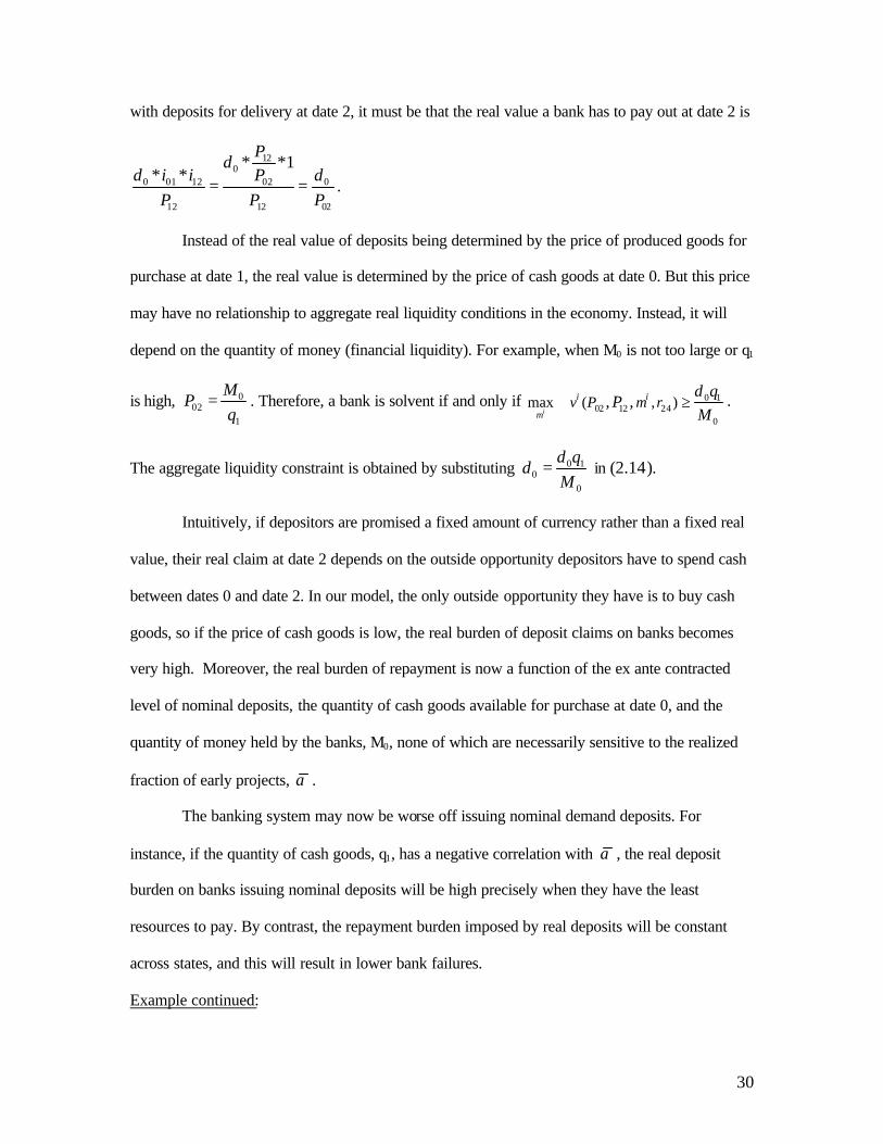
30

with deposits for delivery at date 2, it must be that the real value a bank has to pay out at date 2 is

120

0 01 12 02 0

12 12 02

* *1* *

Pi i PP P P

δδ δ

= = .

Instead of the real value of deposits being determined by the price of produced goods for

purchase at date 1, the real value is determined by the price of cash goods at date 0. But this price

may have no relationship to aggregate real liquidity conditions in the economy. Instead, it will

depend on the quantity of money (financial liquidity). For example, when M0 is not too large or q1

is high, 002

1

MP

q= . Therefore, a bank is solvent if and only if 0 1

02 12 240

max ( , ), ,i

i iv P rq

PMµ

µδ

≥ .

The aggregate liquidity constraint is obtained by substituting 0 10

0

qd

Mδ

= in (2.14).

Intuitively, if depositors are promised a fixed amount of currency rather than a fixed real

value, their real claim at date 2 depends on the outside opportunity depositors have to spend cash

between dates 0 and date 2. In our model, the only outside opportunity they have is to buy cash

goods, so if the price of cash goods is low, the real burden of deposit claims on banks becomes

very high. Moreover, the real burden of repayment is now a function of the ex ante contracted

level of nominal deposits, the quantity of cash goods available for purchase at date 0, and the

quantity of money held by the banks, M0, none of which are necessarily sensitive to the realized

fraction of early projects, α .

The banking system may now be worse off issuing nominal demand deposits. For

instance, if the quantity of cash goods, q1, has a negative correlation with α , the real deposit

burden on banks issuing nominal deposits will be high precisely when they have the least

resources to pay. By contrast, the repayment burden imposed by real deposits will be constant

across states, and this will result in lower bank failures.

Example continued:

31

Returning to our example with Bα =0.25, let the level of nominal deposits be 0δ = 0.933.

With 0 0.2M = and 1 0.3q = , 02 0.66P = and 0

02

1.4Pδ

= . Thus for the initial parameters, the real

burden of deposit repayments is the same as in the previous example, 1.4, and the resulting credit

extended, (1 )Bµ− = 0.43, is the same. It is easily seen from the earlier example that the bank will

now fail if 0.13Bα = , even though it has issued nominal deposits – because the real deposit

burden is now determined by P02 and does not adjust sufficiently with α .

Alternatively, let the available cash goods, 1q , go up to 0.31. Since the price level P02

drops, the real deposit burden increases when the bank has issued nominal deposits, and credit

falls to (1 )Bµ− = 0.38. When 1q goes further up to 0.32, somewhat paradoxically the B type

banks fail reflecting a true curse of plenty. By contrast, when banks have issued real deposits, an

increase in 1q only increases the available goods for date-2 consumption without increasing the

real deposit burden. As a result, available credit increases, first to 0.44 for 1q = 0.31 and then to

0.45 for 1q = 0.32. In sum then, banks that issue nominal deposits can be extremely vulnerable to

changes in outside cash opportunities. Since cash opportunities make nominal demand deposits

effectively real but in a way that their value need not depend on α , the example shows

Proposition 3: So long as money has transactions value, the representative bank’s ability to

survive for some level of α will not guarantee its ability to survive at all levels of α .

3.8. Discussion.

The point we have made is worth elaborating. When a bank offers nominal deposit

contracts, it has to meet an inter-temporal no-arbitrage condition that depends on the state

contingent movement in the price level. Our focus has been on how transactions demand for cash

prevents natural price level adjustments from stabilizing banks from aggregate real shocks. In

addition, as others have noted, unaccommodated shocks to money demand will change the real

32

nominal debt burden (see Calomiris [1988] and Champ, Smith and Williamson [1996]). A low

level of money in the system can make cash transactions extremely lucrative. Even if these

transactions are a minuscule portion of the economy, rates on deposits have to rise to match them

because depositors have the right to withdraw cash. Not only does this make the bank highly

susceptible to fleeting opportunities available in the cash market even if that market is quite

small, it also forces a future real liability on the bank (and a potential aggregate real liquidity

shortage), even if the bank has issued nominal deposits. The nature of the bank’s liabilities is

critical to why it is susceptible to monetary fluctuations.

This point is not just of theoretical interest. It is well known that money and banking are

related, yet the precise connection between tight monetary conditions, aggregate credit, and bank

solvency has been much debated. We provide one possible channel, for which there may be some

historical support. In his monumental history of the Venetian money market, Mueller (1997,

p326) describes how the Senate fixed the time for sailing of the Venetian trading galleys largely

in July and August. This was a time of enormously high transactions demand for money as

merchants strove to buy the goods and bullion to stock the ships with. Not surprisingly, interest

rates were very high during this time. Mueller citing an anonymous merchant manual writes

“…August coincided with fewer deadlines for payments of debts than…July but that the demand for specie for export was so high in the last ten days of the month that the banks were “cooked” by the heat of cash withdrawals; money was dearer in that moment than in the whole rest of the year. As soon as the Alexandria galleys left the port, rates collapsed.”

Not surprisingly, almost all bank failures occurred between July and October (Mueller 1997,

p127).

More recently, the banking system in Argentina had committed to repay depositors in

dollars (effectively real deposits in a peso economy) but the country did not have the dollars, or

could not commit to attract enough of them, to repay depositors. Faced with such a shortage,

banks failed in 2002. The lesson some economists draw from this crisis is that the banking system

should not have issued real (i.e., dollar denominated) deposits.

33

But issuing peso denominated deposits may not be a panacea unless the value of the peso

in terms of both local goods and foreign exchange fully, and at all times, reflect the condition of

the real economy. But if the value of the peso fluctuated in ways that did not reflect the

underlying state of the economy, then the real repayment burden on the banks issuing nominal

deposits would have become much higher than would have been the case if it were fixed in real

terms. For instance, if the peso were temporarily overvalued relative to the dollar, then the

nominal interest rate on pesos would have had to rise to match the real opportunities available to

depositors who could withdraw pesos to buy dollars and then foreign goods. The real repayment

burden on the banks would then become a function of the maximum overvaluation of the

currency, and the health of banks would become hostage to the country’s competence and

credibility in managing its exchange rate. If this were questionable to begin with, the country’s

banking system may have been better off issuing “real” deposits.

IV. The Channels of Transmission of Monetary Policy

4.1. The Channels of Transmission of Monetary Policy: The Liquidity Channel

The previous section suggests that monetary conditions matter because they affect the

real value of deposit liabilities. A current shortage of money relative to cash goods causes an

incipient drain on the banking system, which is averted only if the banks pay depositors a very

high nominal rate. But this increases future bank obligations (aggregate real liquidity demand),

which will be met by increases in the real interest rate, by curtailing credit and restructuring

projects, and by bank failures.

This then suggests a “liquidity” channel through which monetary policy can affect real

economic activity: ultimately it works through prices, interest rates, and bank balance sheets, all

ingredients that have been separately identified by other theories of transmission (see Bernanke

and Gertler (1995) or Kashyap and Stein (1994, 1997) for detailed surveys). But the reason is

different from the traditional ones. Banks are special in transmission not because of reserve

34

requirements, sticky prices, or special guarantees given to deposits, but because their demandable

liabilities are non-renegotiable, and convert to cash on demand. In addition, they have some

control over production of their borrowers.

To see the channel working, consider an open market repurchase conducted by the

monetary authority, which has the effect of increasing the date-0 money supply to 0M + ∆ and

reducing the face value of outstanding date-2 bonds to 2 02B i− ∆ where ∆ is a small number. Let

the open market repurchase be announced after initial contracts are negotiated and projects

initiated, and be executed so that banks have the added money at date 0. To focus on the pure

effect of the open market operation, let no other exogenous parameter be changed at this or other

dates.14 Furthermore, let the parameters be such that at any date -2 price level, the total supply of

consumption goods is not enough to meet the total demand without some restructuring by B type

banks. If the system is in a unique equilibrium where both types of banks survive, we have

Proposition 4: So long as the gross nominal interest rate exceeds 1, the effect of an open market

repurchase of bonds with money at date 0 is to increase the available credit (i.e., reduce the

fraction of late projects restructured).

Proof: See appendix.

So long as 02 1i > , the effect of an increase in money will be to increase 02P (= 0

1

Mq

+ ∆),

reduce the nominal rate, and reduce the required real deposit payout at date 2, 0

02Pδ

. This will

cause real aggregate liquidity demand at date 2 to fall. A reduction of aggregate real liquidity

demand will tend to reduce the fraction of projects liquidated, or equivalently, enhance the supply

of credit. The details of the proof show that changes in prices or interest rates do not offset the

direct effect of the decrease in liquidity demand.

14 This would mean that at date 2, we would have to inject (helicopter drop) a small amount of money,

02( 1)i∆ − to keep the quantity of money constant at 0 2M B+ .

35

Example continued

Consider again our base case example with 0.25Bα = . An increase in the money supply at date

0 from 0.2 to 0.22 increases credit from (1 ) 0.43Bµ− = to (1 ) 0.53Bµ− = .

Corollary 1: When the gross nominal interest rate i02 is 1 (the net nominal interest rate is zero),

an open market repurchase of bonds with money at date 0 will have no effect on the amount of

credit available at date 2.

When the nominal interest rate is 1, money and bonds are equivalent because the

marginal unit of money provides no transaction services while bonds provide no interest – there is

enough money at date 0 that the price of cash goods purchased at that date equals the price of

produced goods at date 1. Any additional money issued by the monetary authority to repurchase

bonds will be held by the banks as a store of value and not withdrawn by investors for date-0

transactions. Open market operations will have no effect on the date-0 price of cash goods, P02,

and none on the real deposit burden on the banks at date 2.

Finally a few notes. Because a significant portion of bank liabilities is convertible on

demand, banks are susceptible to temporary spikes in the transactions demand for money. By

contrast, financial intermediaries with longer maturity liabilities are affected only if a substantial

fraction of their liabilities mature together at a time of high transactions demand. A financial

intermediary with longer-term liabilities that are diversified across maturities will be much less

affected by fluctuations in monetary conditions. Changes in monetary policy will have less of an

effect on the activities of such intermediaries.

Another point worth noting is that what really hurts the banking system is a temporary

deflation, which makes withdrawals attractive. If efforts by the monetary authority to inflate do

not set in immediately (due to sticky prices or other reasons), the anticipation of coming inflation

increases the incipient outflows by depos itors. Far better for the health of banks and for

maintaining steady levels of aggregate credit if a monetary authority is able to tailor money

36

supply to the demands of real activity so as to maintain a stable price level. When such a

monetary authority exists, the risks associated with the issuance of nominal deposits decreases,

implying that a banking system can finance more of its assets with demandable claims.

4.2. The Channels of Transmission of Monetary Policy: The Financial Asset Channel

It is useful to note that there are other channels through which an exchange of money for

bonds can affect the real activity of banks. In particular, it could work by altering the real value of

financial assets on bank balance sheets. Recall we showed that the real value of the claims on the

government held by the banks is

2 4 424

0 2 43

12 2 4

1 { , }tX tX tXr

M B BMax qP M B+ = + +

+ (2.16)

where B4 is the face value of date-4 maturing bonds issued at date 2 and M2 is the quantity of

money left after date-4 maturing bonds are issued (=M0+B2-b24 where b24 is the present value of

the date-4 maturing bonds issued at date 2). Keeping real activity constant, the expression

indicates that as the quantity of bonds B4 that are issued decreases from a level that nearly

absorbs the entire money stock (so that M2 is an infinitesimal amount) to 0, the total value of

government claims held by the banks decreases from 42

24

3 tXtX

rq ++ to

2 424

31 { , }tX tX

rMax q+ .

The decrease in the real value of government claims with expansionary open market

operations is not because of seigniorage (government real revenues are assumed fixed): When

there is only a minuscule amount of money outstanding, not only can current holders of money

buy cash goods at a deeply discounted price, but also government bonds maturing at date 4

account for the lion’s share of the public’s claims on the government, so bonds capture the full

value of real taxes. As the money stock increases, the dealers in the cash market at date 3 no

37

longer have to sell goods for a deeply discounted price. Also bonds have to share the value of real

taxes with holders of money. Therefore, as the amount of money outstanding increases relative to

bonds, and as the nominal rate falls to 1, the real value of government liabilities (money plus

bonds) holding real activity and real rates constant falls.15 Of course, once the nominal rate falls

to one, no further alteration in value is possible, and further open market operations lose all

effect.16

Thus open market operations reduce the real value of government assets held by banks at

date 2, and reduce aggregate liquidity demand by reducing the real value of the bank’s liabilities.

This leads to an expansion in bank credit for similar reasons to the ones discussed in the previous

sub-section. The “financial asset” channel is probably weaker than the “liquidity” channel

because the former works primarily by altering the value of bank liabilities such as capital that are

most sensitive to bank asset values (unlike the latter which works by altering the real value of

deposit payouts). In practice, non-deposit bank liabilities are less likely to be held for liquidity or

transactions purposes, and thus the change in their value will have less of an effect on the

aggregate demand for liquidity.

3.3. Financial Contagion.

Our model offers a stark and transparent way of modeling the use of money in payments.

This allows us to see the effects of alternative assumptions. For instance, suppose depositors who

run on a bank will not accept deposits on other banks but will only take money (for instance,

because they may need time to verify the quality of the bank they will deposit in). With this small

15 Contrast this with the effect on nominal liabilities. Pushing down the nominal interest rate increases the nominal value of bonds and the total nominal value of government claims. 16 Note also that the government’s real revenues are unchanged if real output does not change (and government expenditure is fixed). So substituting interest-bearing liabilities for non-interest bearing ones does not result in a greater real claim on the government or in lower seigniorage profits. There are no sticky prices in our model. Open market operations simply transfer value from one set of agents to others but do not alter the aggregate real future payments by the government.

38

change in assumptions, bank failures can become contagious through their effect on monetary

conditions.

In particular, suppose now that type B banks are not expected to meet their nominal

deposit obligations at date 2 and fail. Then they will be run immediately at date 0. They will pay

out their cash reserves to depositors, but once the B type banks run out, they will have to sell

assets. If the only asset that their depositors will accept is cash, the bank’s assets must be sold for

cash (and not for deposits in other banks). The sale of the bank’s assets will lock up more cash in

transactions, leaving less cash to buy cash goods. This will further depress the price of cash goods

to

002

1 2( )B

MP

q c Bθ=

+ + (2.17)

where the denominator in (2.17) now also includes the value of restructured loans and bonds that

the B type banks sell. This will make the purchase of cash goods even more lucrative, and force

the G type banks to pay a yet higher rate to keep their depositors from moving to cash. 17 Given

the higher effective payout to deposits at date 2, these type G banks could also fail if 0

02

GvPδ

< .

The mechanism here resembles the contagious bank failures described by Friedman and Schwarz

(1963): Depositors run on banks and take money, forcing banks to sell assets for cash, which

renders the money supply inadequate for the quantum of real activity, forcing a further drop in the

price level and still more bank failures.

Conclusion

17 Note that the problem is not the price drop of the assets sold in the fire sale (also present in Diamond [1987] and Allen-Gale [1998]), but the increase in the interest rate required to keep money from being withdrawn for cash purchases.

39

We have introduced money in a real model of banking. Our purpose was to understand

how the supply of money and the availability of bank credit might be tied to each other.

We show that there is a connection between bank lending and monetary conditions,

especially in situations where there is a binding aggregate supply of real liquidity. We show that

monetary intervention can have real effects even in a world without many of the traditional

assumed frictions. We also show that while nominal deposits can, under fairly restrictive

conditions, serve as a natural hedge, in general they do not insulate the bank against adverse

shocks. In fact, a bank that has issued real deposits may be better hedged.

Turning finally to the scope for future work, we have made a number of strong

assumptions to simplify our analysis. Fiscal policy is relatively static in our model. Initial

investors cannot substitute at all for consumption between dates. We have no limitation on

transactions imposed by the availability of deposits in this model. We do not have long dated

bonds. Finally, we do not have agents who are totally outside the banking system. Relaxing each

of these is a realistic and potentially interesting extension that suggests scope for future work.

References

Allen, Franklin and Douglas Gale, [1998] “Optimal Financial Crises,” Journal of Finance 53, 1245 – 1284. Bernanke, Ben S.; Blinder, Alan S. Credit, Money, and Aggregate Demand American Economic Review

v78, n2 (May 1988): 435-39 Bernanke, Ben S. ; Gertler, Mark, “Inside the Black Box: The Credit Channel of Monetary Policy

Transmission,” Journal of Economic Perspectives v9, n4 (Fall 1995): 27-48 Caballero, R, and A. Krishnamurthy [2000], “International Liquidity Management: Sterilization Policy in

Illiquid Financial Markets”, mimeo, MIT. Calomiris, Charles W. [1988], “Institutional Failure Monetary Scarcity and the Depreciation of the Continental, Journal of Economic History 48 (March 1988): 47-68. Calomiris, Charles W. and Charles M. Kahn [1991], “The Role of Demandable Debt in Structuring

Optimal Banking Arrangements” The American Economic Review, Vol. 81, No. 3. (Jun., 1991), pp. 497-513.

Champ, Bruce, Bruce Smith, and Stephen Williamson, 1996. .Currency Elasticity and Banking Panics:

Theory and Evidence,. Canadian Journal of Economics 29, 828-864.

40

Cochrane, John, “Money as Stock,” University of Chicago working paper, 2001, http://www-gsb.uchicago.edu/fac/john.cochrane/research/Papers/cashless2a.pdf Clower, R. [1967] “Reconsideration Of The Microfoundations Of Monetary Theory , Western Economic

Journal 6 (1): 1-8 1967 Diamond, Douglas W. “Liquidity, Banks, and Markets,” Journal of Political Economy, October 1997. Diamond, D. W. and P. H. Dybvig [1983], .Bank Runs, Deposit Insurance, and Liquidity,. Journal of

Political Economy 91, 401-419. Diamond, Douglas W. and Raghuram Rajan A Theory of Bank Capital,. Journal of Finance 55 (December

2000): 2431-2465. Diamond, Douglas W. and Raghuram Rajan “Liquidity risk, liquidity creation and financial fragility: A

theory of banking,” Journal of Political Economy 109 (April 2001a). Diamond, Douglas W. and Raghuram Rajan “Liquidity Shortages and Banking Crises,” University of

Chicago working paper, 2002a. Diamond, Douglas W. and Raghuram Rajan “Bank Bailouts and Aggregate Liquidity,” American

Economic Review, Papers and Proceedings, (May 2002b). Englund. Peter and Lars E. O. Svensson “Money and banking in a cash in advance economy.” International

Economic Review, 29 no. 4, (November 1988): 681-705. Friedman, M and A. Schwartz [1963], A Monetary History of the United States 1867-1960. Princeton:

Princeton Univ Press. Gibson, Michael S. “More Evidence on the Link between Bank Health and Investment in Japan,” Journal of

the Japanese and International Economies v11, n3 (September 1997): 296-310. Gurley, John G., and Shaw, Edward S. 1960. Money in a theory of finance. Washington, D.C.: Brookings

Institution. Jeanne, Olivier, “Debt Maturity and the Global Financial Architecture”, 2000, Working Paper, IMF. Kashyap, Anil K.; Stein, Jeremy C., “The Role of Banks in Monetary Policy: A Survey with Implications

for the European Monetary Union,” Federal Reserve Bank of Chicago Economic Perspectives v21, n5 (Sept.-Oct. 1997): 2-18.

Kashyap, Anil K.; Stein, Jeremy C. “Monetary Policy and Bank Lending,” Studies in Business Cycles,

vol. 29. Chicago and London: University of Chicago Press, 1994): 221-56 Kashyap, Anil K.; Stein, Jeremy C. “The Impact of Monetary Policy on Bank Balance Sheets,” Carnegie-

Rochester Conference Series on Public Policy v42, n0 (June 1995): 151-95. Kashyap, Anil K.; Stein, Jeremy C. “What Do a Million Observations on Banks Say about the

Transmission of Monetary Policy?” American Economic Review v90, n3 (June 2000): 407-28. Kashyap, Anil K.; Stein, Jeremy C. and Wilcox, David W., “Monetary Policy and Credit Conditions:

Evidence from the Composition of External Finance,” American Economic Review v83, n1 (March 1993): 78-98.

Lucas, Robert E. Jr., and Nancy L. Stokey, 1987, .Money and Interest in a Cash-in-Advance Economy.

Econometrica 55, 491-513.

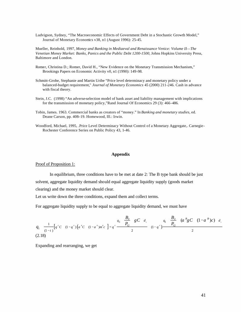
41

Ludvigson, Sydney, “The Macroeconomic Effects of Government Debt in a Stochastic Growth Model,”

Journal of Monetary Economics v38, n1 (August 1996): 25-45. Mueller, Reinhold, 1997, Money and Banking in Mediaeval and Renaissance Venice: Volume II—The Venetian Money Market: Banks, Panics and the Public Debt 1200-1500, Johns Hopkins University Press, Baltimore and London. Romer, Christina D.; Romer, David H., “New Evidence on the Monetary Transmission Mechanism,”

Brookings Papers on Economic Activity v0, n1 (1990): 149-98. Schmitt-Grohe, Stephanie and Martin Uribe “Price level determinacy and monetary policy under a

balanced-budget requirement," Journal of Monetary Economics 45 (2000) 211-246. Cash in advance with fiscal theory.

Stein, J.C. (1998) “An adverse-selection model of bank asset and liability management with implications

for the transmission of monetary policy,”Rand Journal Of Economics 29 (3): 466-486. Tobin, James. 1963. Commercial banks as creators of “money.” In Banking and monetary studies, ed.

Deane Carson, pp. 408–19. Homewood, Ill.: Irwin. Woodford, Michael, 1995, .Price Level Determinacy Without Control of a Monetary Aggregate,. Carnegie-

Rochester Conference Series on Public Policy 43, 1-46.

Appendix

Proof of Proposition 1: In equilibrium, three conditions have to be met at date 2: The B type bank should be just

solvent, aggregate liquidity demand should equal aggregate liquidity supply (goods market

clearing) and the money market should clear.

Let us write down the three conditions, expand them and collect terms.

For aggregate liquidity supply to be equal to aggregate liquidity demand, we must have

( )[ ]2 2

2 21 1

12 121

1(1 ) (1 ) (1

(1 ) 2 2

( (1 ) ))G G B B B G G

B Bq d q d

C C c

B BC C cP P

q θ θ α α µ θ θτ

γ α γ α+ +

+ − + − = + −−

+ + + + + −+

(2.18) Expanding and rearranging, we get

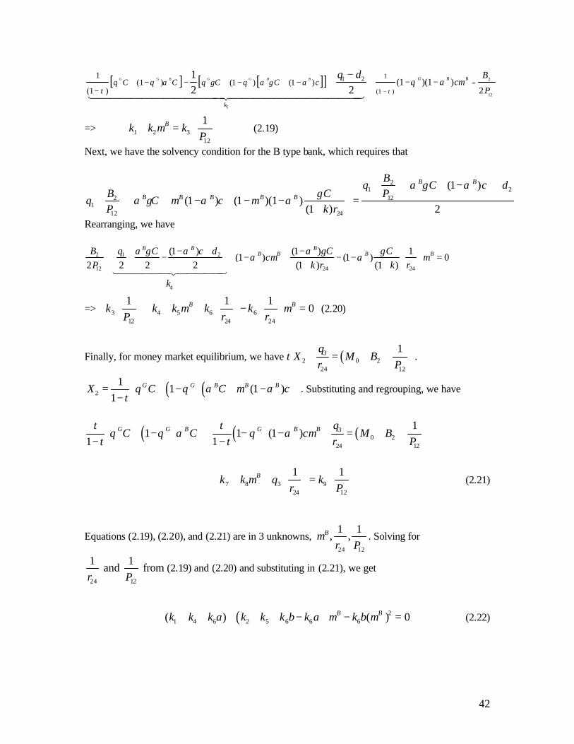
42

[ ] [ ][ ] 2

12

1

1 2 1

(1 )

1(1 ) (1 ) (1 )

(1 )(1 )(1 )

2

12 2

G G B G G B B G B B

k

C C C C cB

cP

q dτ

θ θ α θ γ θ α γ ατ

θ α µ =−

+ − − + − + −−

+ − −−

+144444444444424444444444443

=> 1 2 312

1Bk k kP

µ

+ =

(2.19)

Next, we have the solvency condition for the B type bank, which requires that

21 2

2 121

12 24

(1 )(1 ) (1 )(1 )

(1 ) 2

B B

B B B B B

Bq C c d

B C Pq C c

P k r

α γ αγ

α γ µ α µ α + + + − +

+ + + − + − − = + Rearranging, we have

2 1 2

12 24 24

4

(1 ) (1 ) 1(1 ) (1 ) 0

2 2 2 2 (1 ) (1 )

B B BB B B BB q C c d C C

cP k r k r

k

α γ α α γ γα µ α µ

− + −+ + − + − + − − = + + 1444442444443

=> 3 4 5 6 612 24 24

1 1 10B Bk k k k k

P r rµ µ

+ + + − =

(2.20)

Finally, for money market equilibrium, we have ( )32 0 2

24 12

1qX M B

r Pτ

+ = +

.

( )( )2

11 (1 )

1G G B B BX C C c

tθ θ α µ α = + − + − −

. Substituting and regrouping, we have

( ) ( ) ( )30 2

24 12

11 1 (1 )

1 1G G B G B B qt tC C c M B

t t r Pθ θ α θ α µ

+ − + − − + = + − −

7 8 3 924 12

1 1Bk k q kr P

µ

+ + =

(2.21)

Equations (2.19), (2.20), and (2.21) are in 3 unknowns, 24 12

1 1, ,B

r Pµ . Solving for

24 12

1 1 and from

r P(2.19) and (2.20) and substituting in (2.21), we get

( ) 21 4 6 2 5 6 6 6( ) ( ) 0B Bk k k a k k k b k a k bµ µ+ + + + + − − = (2.22)

43

where 9 91 7 2 8

3 3 3 3

1 1 and b

k ka k k k k

q k q k

= − = −

.

Proof of Proposition 1 (i): Implicitly differentiating (2.22) w.r.t. Gθ , we get

( )51 4 2

6

2 5 6 6 6

( ) 1

( ) 2

B B BG G G G G GB

G B

dkdk dk dk da dbk

d d d d d ddd k k k b k a k b

µ µ µθ θ θ θ θ θµ

θ µ

− + + + + − + =+ + − −

(2.23)

Some tedious but straightforward algebra shows that the numerator is negative, where we use the condition that some restructuring is needed at any price to prove that k1<0. To sign the denominator, note that it is in the form2 BA Bµ + where the quadratic in (2.22) is

2

0B BA B Cµ µ+ + = . Some algebra shows that A<0, C<0 and B>0. Therefore there will be two

positive roots for Bµ . If the equilibrium is unique, the greater root must exceed 1, and the only

feasible root is the smaller root, 2 4

2B B B AC

Aµ

− + −= . This implies 2 0BA Bµ + > so

0B

G

dd

µθ

< or (1 )

0B

G

dd

µθ−

> .

Proof of Proposition 1 (ii): Implicitly differentiating (2.22) w.r.t. Bα , we get

(2.24)

( ) ( ) ( )5 61 4 26

2 5 6 6 6

( ) 1 1

( ) 2

E

B B B B BB B B B B B B

B

B B

dk dkdk dk dk da dba b kd d d d d d d

dd k k k b k a k b

µ µ µ µ µα α α α α α α

µα µ

− + + + + − + + − + =

+ + − −

6444444444447444444444448

Now ( )24

1Ba br

µ+ = and 6

1B

dk Cd k

γα

−=

+, therefore

( ) ( ) ( ) ( ) ( )6

24

1 1 11

B B B BB

dk Ca b c

d k rγ

µ µ µ µα

− + = − − > − −+

whenever r24>R (which is the

case since some restructuring is needed).

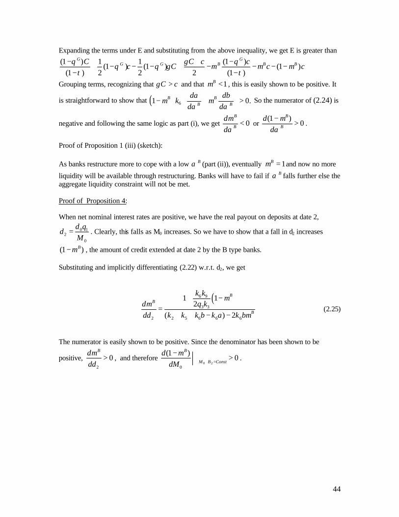
44

Expanding the terms under E and substituting from the above inequality, we get E is greater than

(1 ) 1 1 (1 )(1 ) (1 ) (1 )

(1 ) 2 2 2 (1 )

G GG G B B BC C c c

c C c cθ γ θ

θ θ γ µ µ µτ τ

− + −+ − − − + − − − −

− −

Grouping terms, recognizing that C cγ > and that 1Bµ < , this is easily shown to be positive. It

is straightforward to show that ( ) 61 0.B BB B

da dbk

d dµ µ

α α − + >

So the numerator of (2.24) is

negative and following the same logic as part (i), we get 0B

B

dd

µα

< or (1 )

0B

B

dd

µα−

> .

Proof of Proposition 1 (iii) (sketch): As banks restructure more to cope with a low Bα (part (ii)), eventually 1Bµ = and now no more

liquidity will be available through restructuring. Banks will have to fail if Bα falls further else the aggregate liquidity constraint will not be met. Proof of Proposition 4: When net nominal interest rates are positive, we have the real payout on deposits at date 2,

0 12

0

qd

Mδ

= . Clearly, this falls as M0 increases. So we have to show that a fall in d2 increases

(1 )Bµ− , the amount of credit extended at date 2 by the B type banks. Substituting and implicitly differentiating (2.22) w.r.t. d2, we get

( )6 9

3 3

2 2 5 6 6 6

1 12

( ) 2

BB

B

k kq kd

dd k k k b k a k b

µµ

µ

+ −=

+ + − − (2.25)

The numerator is easily shown to be positive. Since the denominator has been shown to be

positive, 2

0Bd

ddµ

> , and therefore 0 2

0

(1 )0

B

M B Const

ddM

µ+ =

−> .

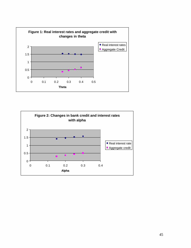
45

Figure 1: Real interest rates and aggregate credit with changes in theta

0

0.5

1

1.5

2

0 0.1 0.2 0.3 0.4 0.5

Theta

Real interest ratesAggregate Credit

Figure 2: Changes in bank credit and interest rates with alpha

0

0.5

1

1.5

2

0 0.1 0.2 0.3 0.4

Alpha

Real interest rateAggregate credit

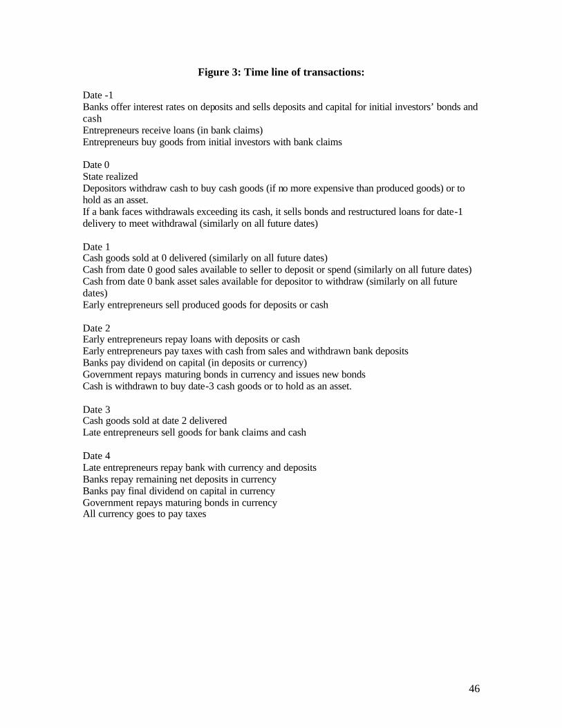
46

Figure 3: Time line of transactions: Date -1 Banks offer interest rates on deposits and sells deposits and capital for initial investors’ bonds and cash Entrepreneurs receive loans (in bank claims) Entrepreneurs buy goods from initial investors with bank claims Date 0 State realized Depositors withdraw cash to buy cash goods (if no more expensive than produced goods) or to hold as an asset. If a bank faces withdrawals exceeding its cash, it sells bonds and restructured loans for date-1 delivery to meet withdrawal (similarly on all future dates) Date 1 Cash goods sold at 0 delivered (similarly on all future dates) Cash from date 0 good sales available to seller to deposit or spend (similarly on all future dates) Cash from date 0 bank asset sales available for depositor to withdraw (similarly on all future dates) Early entrepreneurs sell produced goods for deposits or cash Date 2 Early entrepreneurs repay loans with deposits or cash Early entrepreneurs pay taxes with cash from sales and withdrawn bank deposits Banks pay dividend on capital (in deposits or currency) Government repays maturing bonds in currency and issues new bonds Cash is withdrawn to buy date-3 cash goods or to hold as an asset. Date 3 Cash goods sold at date 2 delivered Late entrepreneurs sell goods for bank claims and cash

Date 4 Late entrepreneurs repay bank with currency and deposits Banks repay remaining net deposits in currency Banks pay final dividend on capital in currency Government repays maturing bonds in currency All currency goes to pay taxes