MONEY DEMAND FUNCTION ESTIMATION BY NONLINEAR COINTEGRATION · MONEY DEMAND FUNCTION ESTIMATION BY...
31
MONEY DEMAND FUNCTION ESTIMATION BY NONLINEAR COINTEGRATION YOUNGSOO BAE † AND ROBERT M. DE JONG ‡ Department of Economics, Ohio State University, USA July 2005 SUMMARY Conventionally, the money demand function is estimated using a regression of the logarithm of money demand on either the interest rate or the logarithm of the interest rate. This equation is presumed to be a cointegrating regression. In this paper, we aim to combine the logarithmic specification, which models the liquidity trap better than a linear model, with the assumption that the interest rate itself is an integrated process. The proposed technique is robust to serial correlation in the errors. For the US, our new technique results in larger coefficient estimates than previous research suggested, and produces superior out-of-sample prediction. JEL Classification: E41; C22 Keywords: Liquidity Trap, Money Demand, Nonlinear Cointegration † Correspondence to: 410 Arps Hall, 1945 North High Street, Columbus OH, 43210, USA. Email: [email protected]. Telephone: 614-292-5765. Fax: 614-292-3906. I would like to thank Masao Ogaki for invaluable advices and encouragement. ‡ Email: [email protected] 1
Transcript of MONEY DEMAND FUNCTION ESTIMATION BY NONLINEAR COINTEGRATION · MONEY DEMAND FUNCTION ESTIMATION BY...

MONEY DEMAND FUNCTION ESTIMATION BY
NONLINEAR COINTEGRATION
YOUNGSOO BAE† AND ROBERT M. DE JONG‡
Department of Economics, Ohio State University, USA
July 2005
SUMMARY
Conventionally, the money demand function is estimated using a regression of the logarithm
of money demand on either the interest rate or the logarithm of the interest rate. This equation
is presumed to be a cointegrating regression. In this paper, we aim to combine the logarithmic
specification, which models the liquidity trap better than a linear model, with the assumption that
the interest rate itself is an integrated process. The proposed technique is robust to serial correlation
in the errors. For the US, our new technique results in larger coefficient estimates than previous
research suggested, and produces superior out-of-sample prediction.
JEL Classification: E41; C22
Keywords: Liquidity Trap, Money Demand, Nonlinear Cointegration
† Correspondence to: 410 Arps Hall, 1945 North High Street, Columbus OH, 43210, USA. Email: [email protected].
Telephone: 614-292-5765. Fax: 614-292-3906. I would like to thank Masao Ogaki for invaluable advices and
encouragement.
‡ Email: [email protected]
1

1 INTRODUCTION
1.1 Money Demand and Functional Form
The money demand function has long been a fundamental building block in macroeconomic mod-
elling and an important framework for monetary policy. The literature on money demand function
estimation is extensive. Most of this literature is concerned with the existence of a stable money
demand function. Notable references are Laidler (1985), Lucas (1988), Hoffman and Rasche (1991),
Miller (1991), Baba et al. (1992), McNown and Wallace (1992), Stock and Watson (1993), Mehra
(1993), Miyao (1996), Ball (2001), and Anderson and Rasche (2001). For a recent literature survey,
see Sriram (2001).
However, much of the recent literature on monetary economics seems to de-emphasize the impor-
tance of money demand; see Duca and VanHoose (2004). Despite the consensus that money demand
function has little role under an interest-rate-based (Taylor-rule type) monetary policy, it is still be-
lieved that money demand is important for both macroeconomic model and monetary policy. This
is especially relevant for countries like Germany, where monetary authorities continue to emphasize
the role of the money demand function on their monetary policy operation. For example, see Beyer
(1998), Lutkepohl et al. (1999), and Coenen and Vega (2001). For the US, Duca and VanHoose(2003)
carefully argue the continued relevance of the money demand function. Their main argument is that
monetary policy does not work only through the interest rate channel, and that money demand can
provide useful information about portfolio allocations.
It should be also noted that in the simultaneous equations framework for the money market,
it has been generally accepted by many researchers that the money supply is largely controlled by
the monetary policy authority. This implies that the money supply curve is vertical in the plane of
the nominal interest rate and the quantity of money. For example, see Papademos and Modigliani
(1990, p.402). Therefore, the money demand function is well identified, and if the money supply is
an integrated process, the money demand function can be estimated by the cointegration method.
In the literature on the estimation of the long-run money demand, the functional form
mt = β0 + β1rt + ut (1)
has been widely used, where mt denotes the logarithm of real money demand and rt is the nominal
interest rate. For example, see Lucas (1988), Stock and Watson (1993) and Ball (2001). In addition
to the functional form of Equation (1), the functional form
mt = β0 + β1 ln(rt) + ut, (2)
2

has been considered, which is based on the inventory-theoretic approach pioneered by Allais (1947,
Vol. 1, pp.235-241), Baumol (1952) and Tobin (1956). In this paper, we consider only the logarithmic
functional form. The motivation for this functional form is as follows. Consider an individual who
receives an income Y in the form of bonds. There is a fixed transactions cost b for converting
interest-bearing bonds into cash. Let K denote the real value of bonds converted into cash each time
there is a conversion. The total transaction costs γ incurred by the individual are given by
γ = b
(Y
K
)+ r
(K
2
),
where the first term represents conversion costs and the second term represents the interest cost on
average money holdings (K/2) over the period. Minimizing the transaction costs with respect to K
yields the following square-root law for optimal real money balances
Md
P=K
2=
1
2
(2bY
r
)1/2
.
Expressing the above equation in logarithmic form, we obtain the following functional form of the
money demand,
ln
(Md
P
)= β0 + β1 ln(Y ) + β2 ln(r), (3)
where the parameters β1 and β2 represent the constant income- and interest-elasticities of money
demand that are implied to be 1/2 by the model. Miller and Orr (1966) extend the Allais-Baumol-
Tobin analysis to the case in which cash flows are stochastic, while maintaining the assumption of a
fixed transaction cost in converting bonds to money. In more recent work Bar-Ilan (1990) extends
the inventory-theoretic model further to allow for the possibility of overdrafting by relaxing the
assumption that the “trigger” be restricted to zero. Money balances may fall below zero and, when
they do, the individual has to pay a penalty at a rate p > 0 for using the overdrafting facility. It is
shown that for any finite nominal interest r and penalty rate p the optimal trigger point is negative.
Only in the special case when the penalty rate of using the credit is infinitely high relative to the
interest rate does the model yield the Allais-Baumol-Tobin result. Since credit and money are very
close substitutes, even small increases in the cost of holding money relative to credit (a higher r/p
ratio) results in substitution of credit for money, thereby yielding a higher interest elasticity of money
demand than the earlier models. Therefore, these extensions by Miller and Orr (1966) and Bar-Ilan
(1990) also give rise to the logarithmic specification of Equation (3), but with a higher value for β2.
3
1.2 Functional Forms of Money Demand, Liquidity Trap and Monetary
Policy
A second motivation for considering a logarithmic specification is the ability to capture the liquidity
trap. The choice of functional form has important implications for the presence of the liquidity trap.
Goldfeld and Sichel (1990, p.346) mentioned that “The issue of functional form for the interest
rate has, of course, a much longer history in the money demand literature, stemming from debates
about the existence of a liquidity trap.” The liquidity trap is the phenomenon where the public’s
money demand becomes indefinite at a low interest rate; that is, the public is willing to hold any
amount of money at a low interest rate, because it is indifferent between money and other financial
assets.1 In the functional form of Equation (1), there is no liquidity trap, while the liquidity trap
exists in the functional form of Equation (2). This is because in the latter specification, the money
demand increases into infinity as the interest rate approaches to zero. Laidler (1985, p.53) argued
that “[Keynes’s analysis] ... suggest that it [money demand] cannot be treated as a simple, stable,
approximately linear, negative relationship with respect to the rate of interest.”
The presence of the liquidity trap has important implications for monetary policy. As Krugman
(1998) pointed out,2 the liquidity trap makes the traditional monetary policy impotent when interest
rate is close to zero. Furthermore, the possibility of the liquidity trap makes a central bank’s optimal
policy different even at the normal range of the interest rate. Nishiyama (2003) showed that in the
presence of the liquidity trap the optimal monetary policy is to set a small but positive inflation rate
as its target, to avoid the possibility of falling into the liquidity trap. This is an important issue
considering US’s current interest rate level that is historically low in 45 years and Japan’s decade of
economic slump despite of almost zero interest rate.3
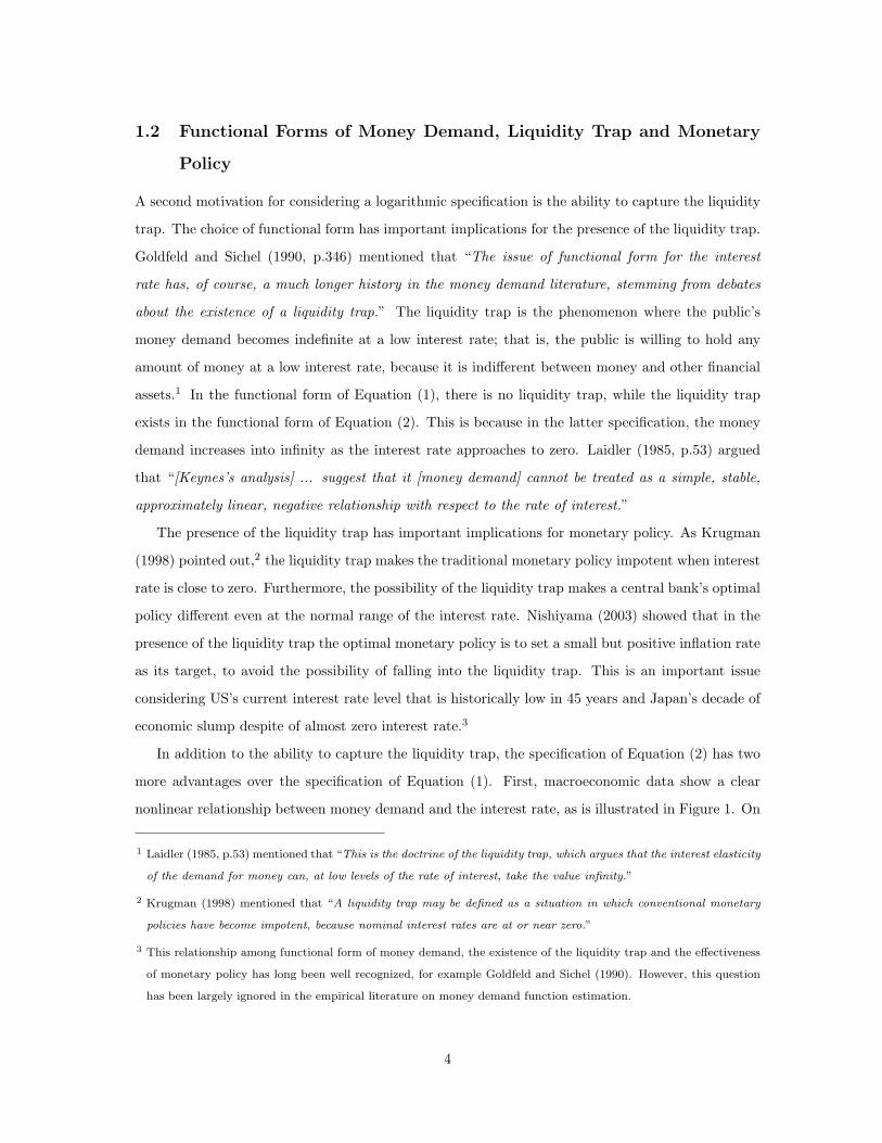
In addition to the ability to capture the liquidity trap, the specification of Equation (2) has two
more advantages over the specification of Equation (1). First, macroeconomic data show a clear
nonlinear relationship between money demand and the interest rate, as is illustrated in Figure 1. On
1 Laidler (1985, p.53) mentioned that “This is the doctrine of the liquidity trap, which argues that the interest elasticity
of the demand for money can, at low levels of the rate of interest, take the value infinity.”
2 Krugman (1998) mentioned that “A liquidity trap may be defined as a situation in which conventional monetary
policies have become impotent, because nominal interest rates are at or near zero.”
3 This relationship among functional form of money demand, the existence of the liquidity trap and the effectiveness
of monetary policy has long been well recognized, for example Goldfeld and Sichel (1990). However, this question
has been largely ignored in the empirical literature on money demand function estimation.
4

the other hand, a graph of the relationship between money demand and the logarithm of the interest
rate appears to be linear. Second, as argued by Anderson and Rasche (2001), the elasticity of money
demand with respect to the interest rate should not be an increasing function of the interest rate, but
it should be a decreasing or at least a non-increasing function. This is because as the public reduces
its money holdings, each successive reduction should not be less difficult. While the interest elasticity
of money demand is an increasing function of the interest rate in the specification of Equation (1),
it is constant in the specification of Equation (2). Considering all these aspects, we may conclude
that the specification of Equation (2) is more appropriate than the specification of Equation (1).
1.3 Linear Cointegration Methods
It is believed by many researchers that the nominal interest rate is an integrated process. This
assumption was made in e.g. Stock and Watson (1993), Ball (2001), Anderson and Rasche (2001),
and Hu and Phillips (2004). See Hu and Phillips (2004) for an argument for nonstationarity in the
nominal interest rate. This assumption might have some advantages over the alternative assumption
that the logarithm of the nominal interest rate is an integrated process. In the latter assumption,
the nominal interest rate is an exponential function of an integrated process, which implies that
its percentage change has a stationary distribution. This might be an appropriate assumption for
some macroeconomic variables, such as GDP and CPI. For the nominal interest rate, however, if we
consider the fact that the Federal Reserve Board (FRB) usually adjusts its target interest rate by
multiples of 25 basis points, not by certain percentage of the current interest rate level, it might be
more appropriate to assume that its difference has a stationary distribution, which in turn implies
that the nominal interest rate itself is an integrated process.
Under the assumption that the nominal interest rate is an integrated process, cointegration
methods have been used for the estimation and the statistical inference on the money demand
function. However, to use conventional linear cointegration methods, such as Phillips and Hansen
(1990)’s “Fully Modified OLS” (FMOLS) and Stock and Watson (1993)’s “Dynamic OLS” (DOLS),
we need to make different assumptions for different functional forms; that is, for Equation (1), rt
must be assumed to be an integrated process, and for Equation (2), ln(rt) must be assumed to
be an integrated process. However, if rt is an integrated process, then the logarithm of rt is not
5

an integrated process in any meaningful sense, and vice versa.4 Because of this problem, linear
cointegration methods do not provide a consistent framework to estimate both Equation (1) and (2)
under the assumption that the interest rate is an integrated process. The approach in this paper
seeks to estimate the functional form of Equation (2) under the assumption that the interest rate is
an integrated process; that is, we aim to reconcile the assumption that interest rate is an integrated
process with the logarithmic functional form.
Nonlinearity in the short-run dynamics of the money demand function estimation has been inves-
tigated in the framework of “Error Correction Model” (ECM) and “Smooth Transition Regression”
(STR) models; for example, see Terasvirta and Eliasson (2001) and Chen and Wu (2005). How-
ever, to the best of our knowledge, our paper is the first attempt to investigate nonlinearity in the
long-run cointegration relationship of the money demand function. Recently there have been new
developments of nonlinear cointegration methods; notably, Park and Phillips (1999, 2001), Chang
et al. (2001), and de Jong (2002). However, currently available nonlinear cointegration methods
are not suitable for the analysis of the model of Equation (2). The techniques of Park and Phillips
(1999, 2001) and Chang et al. (2001) can be used in principle, but only if we assume that the error
term ut is a martingale difference sequence. Because of the presence of serial correlation and possible
endogeneity, this assumption is not acceptable for estimation of the long-run money demand func-
tion estimation. De Jong (2002) relaxes the martingale difference sequence assumption, however, his
technique cannot be used for the specification of Equation (2) because of the unboundedness of the
logarithm function near zero.
To this end, we will develop a new nonlinear “fully modified” type cointegration method that can
be used in the functional form of Equation (2) under the assumption that rt is an integrated process.
Of course, the assumption of a logarithmic specification in combination with the presence of a unit
root in rt will give rise to the inner inconsistency that integrated processes can take on negative
values. This is not a problem only for Equation (2). In Equation (1), the interest rate cannot be an
integrated process, because it is always positive. This is true for some other macroeconomic variables
as well, such as the unemployment rate. Therefore, in the sequel of this paper it is presumed that
Equation (2) is approximated by a logarithm function of the absolute value of the interest rate.
4 Anderson and Rasche (2001) estimated three different functional forms, such as linear, logarithm and reciprocal
function of the nominal interest rate, by the conventional linear cointegration methods, and concluded that functional
forms of logarithm and reciprocal are more stable than linear one. However, since they used the conventional
linear cointegration for all three different functional forms, their conclusion could not be free from the criticism of
misspecification.
6

Since asymptotic theory provides us with nothing more than approximations to true coefficient
distributions, this paper should be viewed as providing a different means of conducting inference in
the money demand function of Equation (2), using a different approximation of the limit distributions
of coefficients.
The paper is organized as follows. In Section 2, a new nonlinear cointegration method is proposed
and its asymptotic properties are established. In Section 3, the US long-run money demand function
is estimated using both the newly proposed technique and more conventional techniques, and the
estimation results are presented. The conclusions can be found in Section 4.
2 NONLINEAR COINTEGRATING REGRESSION
2.1 Model and Assumptions
In this paper, the nonlinear cointegrating regression
yt = β0 + β1 ln |xt| + ut (4)
is considered, where xt is an integrated process and ut is a stationary process. Note that Equation
(4) is different from Equation (2); i.e. the absolute value of an integrated process |xt| goes into a
logarithm function in Equation (4), not xt. Its estimation and statistical inference are not simple
tasks. To illustrate analytical difficulties that Equation (4) poses, we investigate the properties of
the OLS estimator. The OLS estimator β1 satisfies
√n(β1 − β1) =
1√n
∑nt=1(ln |xt| − ln |xt|)ut
1n
∑nt=1(ln |xt| − ln |xt|)2
=
1√n
∑nt=1(ln
∣∣∣ xt√n
∣∣∣− ln∣∣∣ xt√
n
∣∣∣)ut
1n
∑nt=1(ln
∣∣∣ xt√n
∣∣∣− ln∣∣∣ xt√
n
∣∣∣)2,
where Xt indicates the sample average of Xt. Note that if ut is a martingale difference sequence
as in Park and Phillips (2001), it can be shown that√n(β1 − β1) is Op(1). However, if ut has
serial correlation, and ut and ∆xt are correlated with each other, de Jong (2002) has shown that for
continuously differentiable function T (·),1√n
n∑
t=1
T (xt√n
)utd−→∫ 1
0
T (W (r))dU(r) + Λ
∫ 1
0
T ′(W (r))dr
where W (r) and U(r) are the limiting Brownian processes associated with (∆xt, ut), and Λ is
the correlation parameter. Since∫ 1
01
|W (r)|dr is undefined, it can be conjectured that if Λ 6= 0,
1√n
∑nt=1 ln
∣∣∣ xt√n
∣∣∣ut has no well-defined limit, and therefore√n(β1 − β1) does not converge in distri-
bution.
Throughout the paper, the following assumptions are maintained.
7

Assumption 1 Let ∆xt = wt with x0 = Op(1). ut and wt are linear processes
ut =
∞∑
i=0
φ1,iε1,t−i
wt =
∞∑
i=0
φ2,iε2,t−i,
where εt = (ε1,t, ε2,t) is a sequence of independent and identically distributed (i.i.d.) random variables
with mean zero. The long-run covariance matrix of ηt = (ut, wt), Ω, is given by
Ω = C0 +∞∑
j=1
(Cj + C ′j) =
Ω11 Ω12
Ω21 Ω22
where Cj = E(ηtη′t−j). Ω22 is nonsingular.
Note that ut and wt are allowed to be weakly dependent and correlated with each other.
Assumption 2∑∞
i=0 i|φj,i| <∞ and E|εj,t|p <∞ for some p > 2 for j = 1, 2.
Assumption 3 The distribution of (ε1,t, ε2,t) is absolutely continuous with respect to the Lebesgue
measure and has characteristic function ψ(s) for which lim|s|→∞ |s|qψ(|s|) = 0 for some q > 1.
Under Assumption 1, 2 and 3, 1√t
∑ti=1 wi has a density ft(·) that is uniformly bounded over t.
Also, define
Un(r) =1√n
[nr]∑
t=1
ut
Wn(r) =1√n
[nr]∑
t=1
wt,
where [s] denotes the largest integer not exceeding s. Then we can assume without loss of generality
that by the Skorokhod representation theorem,
supr∈[0,1]
|Wn(r) −W (r)| = o(1)
and
supr∈[0,1]
|Un(r) − U(r)| = o(δn),
where δn is a deterministic sequence that is o(n−p−22p ); see Park and Phillips (1999, p.271).
8

2.2 Estimation
In this section, a “Nonlinear Cointegration Least Squares” (NCLS) estimator β1 is defined and
its asymptotic properties are established. This estimator solves the problems associated with the
unboundedness of the logarithm function near zero that make the OLS estimator intractable for
analysis. Let kn be an integer-valued positive sequence such that kn → ∞ and knn− p−2
3p+η → 0 for
some η > 0, and nj =[
njkn
]for j = 0, 1, 2, . . . , kn. Let zt = ln |xnj−1+1| for nj−1 + 1 ≤ t ≤ nj for
j = 1, 2, . . . , kn. Then the NCLS estimator β1 is
β1 =
∑nt=1 zt(yt − yt)∑n
t=1 zt(ln |xt| − ln |xt|)=
∑kn
j=1
∑nj
t=nj−1+1 ln |xnj−1+1|(yt − yt)∑kn
j=1
∑nj
t=nj−1+1 ln |xnj−1+1|(ln |xt| − ln |xt|).
This is an IV estimator that uses zt as the instrumental variable for ln |xt|. Note that kn → ∞ at a
slower rate than n, and kn = o(n1/3) when p = ∞.
Two technical results that are needed in the sequel are stated below.
Theorem 1 Under Assumption 1, 2 and 3,
1√n
kn∑
j=1
nj∑
t=nj−1+1
ln
∣∣∣∣xnj−1+1√
n
∣∣∣∣utd−→∫ 1
0
ln |W (r)|dU(r).
Theorem 2 Under Assumption 1, 2 and 3,
1
n
kn∑
j=1
nj∑
t=nj−1+1
ln
∣∣∣∣xnj−1+1√
n
∣∣∣∣ ln∣∣∣∣xt√n
∣∣∣∣d−→∫ 1
0
[ln |W (r)|]2dr.
Based on Theorem 1 and 2, the asymptotic distribution of β1 is obtained in the following theorem.
Theorem 3 Under Assumption 1, 2 and 3,
√n(β1 − β1)
d−→
∫ 1
0
ln |W (r)|dU(r) − U(1)
∫ 1
0
ln |W (r)|dr∫ 1
0
[ln |W (r)|]2dr −[∫ 1
0
ln |W (r)|dr]2 .
The result of Theorem 3 is reminiscent of the limit theory for the least squares estimator in a linear
cointegration regression. In both cases, the result holds without exogeneity assumption of any kind,
and the limit distribution is not directly suitable for inference in some empirical settings. If W (·) and
9

U(·) are orthogonal, then the usual “t- and F -statistics” are valid because they achieve the correct
significance level conditionally on W (·). However, if they are not orthogonal, which is likely in the
long-run money demand function case, this result cannot be used for the statistical inference, since
the above limit distribution depends on the correlation between U(·) and W (·).
2.3 Fully Modified Type Estimation of the NCLS Estimator
In this section, a “fully modified” type estimation procedure for the NCLS estimator is proposed. A
modification is needed to establish the asymptotic conditional normality. The regression Equation
(4) can be written as
y†t = β0 + β1 ln |xt| + u†t , (5)
where y†t = yt−Ω′21Ω
−122 ∆xt and u†t = ut−Ω′
21Ω−122 ∆xt. Note that now the limiting Brownian process
associated with u†t , U†(·), and W (·) are orthogonal.5
The proposed estimation procedure is now as follows.
1. Calculate the residual, ut, from a regression of yt on an intercept and ln |xt| by the NCLS
estimation method.
2. Get a HAC estimate Ω by using (ut, ∆xt).
3. Calculate y†t in a way analogous to FMOLS,
y†t = yt − Ω′21Ω
−122 ∆xt.
4. The “fully modified” NCLS estimator β1 is defined as the NCLS estimator that is calculated
using the modified dependent variable y†t , instead of yt, i.e.
β1 =
∑nt=1 zt(y
†t − y†t )∑n
t=1 zt(ln |xt| − ln |xt|)=
∑kn
j=1
∑nj
t=nj−1+1 ln |xnj−1+1|(y†t − y†t )∑kn
j=1
∑nj
t=nj−1+1 ln |xnj−1+1|(ln |xt| − ln |xt|).
5 This follows because
limn→∞
E
0 1√
n
[rn]Xt=1
u†t
1A0 1√
n
[rn]Xt=1
∆xt
1A= lim
n→∞E
0 1√
n
[rn]Xt=1
ut
1A0 1√
n
[rn]Xt=1
∆xt
1A− Ω′21Ω−1
22 E
0 1√
n
[rn]Xt=1
∆xt
1A2
= Ω′21 − Ω′
21Ω−122 Ω22 = 0.
10

To establish the asymptotic distribution of β1, the following additional assumption is needed.
Assumption 4 Let k(·) and bn : n ≥ 1 be a kernel function and a sequence of bandwidth para-
meters that are used for the HAC estimator Ω in step 2.
(i) k(0) = 1, k(·) is continuous at zero, and supx≥0
|k(x)| <∞.
(ii)
∫ ∞
0
k(x)dx <∞, where k(x) = supy≥x
|k(y)|.
(iii) bn ⊆ (0,∞) and limn→∞
(1
bn+
bn√n
)= 0.
Assumption 4 is Assumptions A3 and A4 in Jansson (2002, p.1450). Note that Assumption 4 (i)
and (ii) hold for the 15 kernels, including the Bartlett kernel, studied by Ng and Perron (1996), and
Assumption 4 (iii) holds whenever the bandwidth expansion rate coincides with the optimal rate in
Andrews (1991); see Jansson (2002, p.1450-1451).
The following results establishes the consistency of the HAC estimator Ω.
Theorem 4 Let Ω be the HAC estimator in Step 2. Under Assumption 1, 2, 3 and 4, Ωp−→ Ω.
The asymptotic distribution of the “fully modified” NCLS estimator β1 is obtained in the following
theorem.
Theorem 5 Under Assumption 1, 2, 3 and 4,
√n(β1 − β1)
d−→
∫ 1
0
ln |W (r)|dU†(r) − U†(1)
∫ 1
0
ln |W (r)|dr∫ 1
0
[ln |W (r)|]2dr −[∫ 1
0
ln |W (r)|dr]2 .
Since W (r) and U†(r) are orthogonal in Theorem 5, it follows that conditionally on W (·),
√n(β1 − β1)
d−→ N
0,
Ω†11∫ 1
0
[ln |W (r)|]2dr −[∫ 1
0
ln |W (r)|dr]2
,
where Ω†11 is the long-run variance of u†t . This implies that the usual “t- and F -statistics” are valid.
For estimation of Ω†11, a consistent estimator Ω†
11 is provided by
Ω†11 = Ω11 − Ω′
21Ω−122 Ω21.
Note that since Ωp−→ Ω by Theorem 4, Ω†
11 is a consistent estimator for Ω†11.
11

2.4 Sensitivity to the Choice of kn
In order to assess the sensitivity of our estimator β1 to different values of kn, we carried out an
informal and limited simulation study. The simulation procedure was as follows:
1. Generate (∆xt, ut) for t = 1, . . . , n = 100 using the following VAR(1) model with initial value
(∆x0, u0) = (0, 0):
∆xt
ut
=
φ11 φ12
φ21 φ22
∆xt−1
ut−1
+
ε1,t
ε2,t
,
where (ε1,t, ε2,t) is bivariate normal with mean zero and variances σ21 and σ2
2 , and ε1,t and ε2,t
are independent.
2. Construct data yt using the nonlinear cointegrating regression
yt = β0 + β1 ln |xt| + ut.
3. Estimate β1 using our “fully modified” NCLS estimation method with different values for kn.
4. Repeat Step 1-3 100,000 times and compute the average of β1 for each value of kn.
For β0, β1, σ21 and σ2
2 , we use the values that are estimated from actual US data; for the details
of the simulation parameter specifications, see footnote (1) below Table 5. For the choice of the φij ,
however, we consider five different combinations, including one that is estimated from actual US data
as a benchmark case. Simulation results in Table 5 indicate that our NCLS estimator is generally
robust to the different values of kn, although the mean squared error increases as n/kn increases.
3 US MONEY DEMAND
In this section, the US long-run money demand functions of Equation (1) and (2) are estimated
by both linear and nonlinear cointegration methods. Specifically, we use “Static OLS” (SOLS),
DOLS, FMOLS, and NCLS estimation techniques.
3.1 Unit Root Test Results
We first conduct unit root tests for the nominal interest rate and the logarithm of the nominal
interest rate by both the Augmented Dickey-Fuller (ADF) test and Kwiatkowski-Phillips-Schmidt-
Shin (KPSS) test (Kwiatkowski et al. 1992). Test results are presented in Table 1. The ADF test
results show that the null hypotheses that rt and ln(rt) are integrated processes without drift cannot
12

be rejected, and the KPSS test results show that the null hypotheses that rt and ln(rt) are stationary
processes are rejected. Therefore, both tests confirm the hypotheses that rt and ln(rt) are integrated
processes.
3.2 Estimation Results
The same data set as Ball (2001), Stock and Watson (1993) and Lucas (1978) is used, however it was
extended up to 1997.6 M17, Net National Products (NNP), NNP deflator, and 6-months commercial
paper rate are used as money, output, price, and nominal interest rate, respectively.
Coefficient estimates and their HAC asymptotic standard deviations are presented in Table 2.
When the estimation results are compared between linear cointegration methods and the NCLS
method in the functional form of Equation (2), the NCLS estimates are larger in absolute value than
all other linear cointegration estimates when the bandwidth parameter kn is small. Note that the
theory for the NCLS estimator is valid for kn = o(n13 ) at best, which suggests that a small value for
kn may be appropriate. Also, note that for kn = 7, all NCLS point estimates are outside all the 95%
confidence intervals suggested by the SOLS, DOLS and FMOLS estimates.
To further address the question which functional form is most appropriate and which estima-
tion technique is to be preferred, we investigate out-of-sample prediction performance in terms of
sum of squared forecast errors. Results are presented in Table 3 and 4. Between the functional
forms of Equation (1) and (2), Equation (2) outperforms Equation (1) in all combinations of differ-
ent estimation methods and prediction methods. Within the functional form of Equation (2), the
NCLS estimator produces superior prediction performance compared to other conventional linear
cointegration estimators. The superior out-of-sample prediction performance of the NCLS estimator
in combination with the logarithmic specification suggests that the NCLS technique produces the
most desirable estimation results, and this reinforces our belief that the conventional techniques may
underestimate the impact of the nominal interest rate on money demand.
6 The reason data extension is stopped in 1997 is that 6-months commercial paper rate was discontinued at that
point.
7 After 1995, the official M1 statistics excludes the Sweep Account. As shown by Dutkowsky and Cynamon (2003),
this might have an impact on cointegration relationship. Therefore, we added the Sweep Account to M1 from 1994.
13

4 CONCLUSION
This paper investigates two different functional forms for the US long-run money demand func-
tion by linear and nonlinear cointegration methods. Since different functional forms have different
implications for the presence of the liquidity trap and effectiveness of the traditional monetary policy,
the choice of functional form is an important issue. Therefore, its estimation should be conducted
in a consistent framework so that estimation results can be comparable. Since a logarithm function
involves a nonlinear relationship between money demand and the interest rate, nonlinear cointe-
gration methods are more appropriate if the interest rate is presumed to be an integrated process.
This paper proposes a new nonlinear cointegration method that is suitable for a more general time
series situation, such as the long-run money demand function estimation, where serial correlation in
the errors is present. One interesting finding from a theoretical point of view is that our nonlinear
cointegration method establishes√n-consistency of the slope parameter, rather than n-consistency.
Our empirical findings are different from the previous literature in two respects. First, our NCLS
estimates of the nominal interest rate coefficient are larger in absolute value than estimates from
the conventional linear cointegration methods. This implies that the US long-run money demand
function might be more elastic in terms of the nominal interest rate than previously assumed. Second,
our NCLS estimation method avoids a possible misspecification problem that may have existed in the
previous literature where both linear and logarithm specifications were estimated by the conventional
linear cointegration method. Unlike linear cointegration methods, our estimation method has no
theoretical problem. With our new estimation method, we find that the out-of-sample prediction
performance for our NCLS technique is superior to that of conventional linear estimation techniques.
14

5 Appendix
5.1 Estimation Results
Figure 1: Money Demand - Linear vs. Logarithm
15

Table 1: Unit Root Test for Interest Rate1
rt ∆rt ln(rt) ∆ ln(rt)
ADF test2 -0.07 -1.39∗∗ -0.05 -1.04∗∗
KPSS test3 0.64∗ 0.07 0.50∗ 0.13
1 Reject the null hypothesis at 5%(*) and 1%(**).
2 H0: I(1) vs. H1: I(0). The order of the first difference terms is 4.
3 H0: I(0) vs. H1: I(1).
Table 2: Estimation1 Results of Interest Rate Coefficient β1
sample
period
SOLS DOLS2 FMOLS NCLS
(kn = 20)3
NCLS
(kn = 10)3
NCLS
(kn = 7)3
mt = β0 + β1rt + ut
1900-1997 -0.0914 -0.1138 -0.1050 – – –
(0.0100) (0.0074) (0.0097)
1900-1945 -0.0751 -0.0824 -0.0807 – – –
(0.0114) (0.0131) (0.0114)
1946-1997 -0.0910 -0.1054 -0.1045 – – –
(0.0149) (0.0097) (0.0138)
mt = β0 + β1 ln(rt) + ut
1900-1997 -0.3326 -0.3793 -0.3557 -0.3548 -0.4165 -0.5198
(0.0400) (0.0352) (0.0383) (0.0396) (0.0431) (0.0604)
1900-1945 -0.1869 -0.1898 -0.1895 -0.1902 -0.2276 -0.1603
(0.0247) (0.0283) (0.0251) (0.0250) (0.0286) (0.0270)
1946-1997 -0.4863 -0.5140 -0.5089 -0.5196 -0.5908 -0.5977
(0.0474) (0.0397) (0.0447) (0.0463) (0.0468) (0.0528)
1 Numbers in parenthesis are HAC standard error estimates with Bartlett kernel and
bandwidth parameter of 4.
2 The order of the leads and lags is 4.
3 It is equivalent to set n/kn = 5, 10 and 15, respectively.
16

Table 3: Out-of-sample Prediction Performance Results using estimates from 1900-19891
SOLS DOLS FMOLS NCLS (kn = 7)
mt = β0 + β1rt + ut
1997Xt=1990
[mt − bmt]2 1.0439 0.9529 1.0191 –
mt = β0 + β1 ln(rt) + ut
1997Xt=1990
[mt − bmt]2 0.7411 0.6486 0.7056 0.5346
1 The same kernel, bandwidth and order of leads and lags as in Table 2 are used.
Table 4: Out-of-sample One-step-ahead Prediction Performance Results1
SOLS DOLS FMOLS NCLS (kn = 7)
mt = β0 + β1rt + ut
1997Xt=1994
[mt − bmt]2 0.3021 0.2774 0.2790 –
1997Xt=1993
[mt − bmt]2 0.5319 0.5345 0.5246 –
1997Xt=1992
[mt − bmt]2 0.7799 0.7963 0.7825 –
1997Xt=1991
[mt − bmt]2 0.9242 0.9202 0.9165 –
1997Xt=1990
[mt − bmt]2 0.9758 0.9423 0.9517 –
mt = β0 + β1 ln(rt) + ut
1997Xt=1994
[mt − bmt]2 0.1864 0.1567 0.1693 0.0833
1997Xt=1993
[mt − bmt]2 0.3377 0.3096 0.3213 0.2456
1997Xt=1992
[mt − bmt]2 0.5017 0.4689 0.4838 0.4027
1997Xt=1991
[mt − bmt]2 0.6121 0.5632 0.5871 0.4681
1997Xt=1990
[mt − bmt]2 0.6846 0.6165 0.6506 0.4886
1 The same kernel, bandwidth and order of leads and lags as in Table 2 are used.
17

Table 5: Simulation: Sensitivity of the NCLS estimator β1 to Different Values of kn1
n/kn
1 3 5 7 9 11 13 15
φ11 = 0.17, φ12 = −0.84 Mean -0.333 -0.333 -0.333 -0.332 -0.332 -0.363 -0.309 -0.302
φ21 = 0.01, φ22 = 0.86 MSE (0.002) (0.003) (0.004) (0.005) (0.054) (6.731) (2.261) (20.29)
φ11 = 0.0, φ12 = 0.0 Mean -0.333 -0.332 -0.333 -0.334 -0.339 -0.333 -0.343 -0.338
φ21 = 0.0, φ22 = 0.0 MSE (0.000) (0.000) (0.000) (0.005) (0.380) (0.007) (2.299) (1.107)
φ11 = 0.2, φ12 = 0.0 Mean -0.333 -0.332 -0.332 -0.332 -0.333 -0.334 -0.324 -0.333
φ21 = 0.0, φ22 = 0.2 MSE (0.000) (0.000) (0.000) (0.001) (0.007) (0.008) (0.867) (0.057)
φ11 = 0.5, φ12 = 0.0 Mean -0.333 -0.332 -0.332 -0.333 -0.333 -0.330 -0.313 -0.269
φ21 = 0.0, φ22 = 0.5 MSE (0.000) (0.000) (0.000) (0.002) (0.026) (0.022) (1.788) (44.58)
φ11 = 0.5, φ12 = 0.3 Mean -0.333 -0.333 -0.333 -0.333 -0.333 -0.299 -0.367 -0.335
φ21 = 0.3, φ22 = 0.5 MSE (0.010) (0.014) (0.010) (0.009) (0.018) (8.318) (8.600) (22.60)
1 Number of observations n = 100 and number of iterations = 100, 000. β0 = −0.8879 and β1 =
−0.3326. std(ε1) = 1.220 and std(ε2) = 0.076.
18

5.2 Proofs
Proof of Theorem 1: Let kn and nj be same as in Section 2.2. For notational simplicity, let vt+1 =
ut for t = 0, 1, 2, . . . , n, and define Vn(r) = 1√n
∑[nr]t=0 vt+1. Let rj =
nj+1n for j = 0, 1, 2, . . . , kn.
Consider
Gn =1√n
kn∑
j=1
nj∑
t=nj−1+1
ln
∣∣∣∣xnj−1+1√
n
∣∣∣∣ut =1√n
kn∑
j=1
nj∑
t=nj−1+1
ln
∣∣∣∣xnj−1+1√
n
∣∣∣∣ vt+1
=
kn∑
j=1
ln |Wn(rj−1)| (Vn(rj) − Vn(rj−1)) .
Then Gn can be written as
Gn = (Gn − Pn) + (Pn − I) + I
where
Pn =
kn∑
j=1
ln |W (rj−1)|(V (rj) − V (rj−1)) =
kn∑
j=1
∫ rj
rj−1
ln |W (rj−1)|dV (r)
and
I =
∫ 1
0
ln |W (r)|dV (r) =
∫ 1
0
ln |W (r)|dU(r).
Then the theorem can be proved by showing that
|Gn − Pn| p−→ 0
and
|Pn − I| p−→ 0.
First, by summation by parts as in Davidson (1994, p.512), Gn − Pn can be written as
Gn − Pn =
kn∑
j=1
(ln |Wn(rj−1)| − ln |W (rj−1)|)(Vn(rj) − Vn(rj−1)) (1)
+ ln |W (rkn)|(Vn(rkn
) − V (rkn)) (2)
−kn∑
j=1
(Vn(rj) − V (rj))(ln |W (rj)| − ln |W (rj−1)|). (3)
It will be shown that all three terms converge to 0 in probability. For (1),
kn∑
j=1
(ln |Wn(rj−1)| − ln |W (rj−1)|)(Vn(rj) − Vn(rj−1))
2
≤kn∑
j=1
[ln |Wn(rj−1)| − ln |W (rj−1)|]2kn∑
j=1
[Vn(rj) − Vn(rj−1)]2.
19

Now note that
E
kn∑
j=1
[Vn(rj) − Vn(rj−1)]2 = O(1)
because Assumption 1, 2 and 3 imply that E[Vn(rj) − Vn(rj−1)]2 ≤ C · (rj − rj−1). Therefore it
suffices to show that
kn∑
j=1
[ln |Wn(rj−1)| − ln |W (rj−1)|]2 = op(1).
Let Tε(x) = ln |x|I(|x| > ε) + ln(ε)I(|x| ≤ ε), Qε(x) = (ln(ε) − ln |x|)I(|x| < ε), and εn = n−p−23p .
First note that since (a+ b)2 ≤ 2a2 + 2b2, it follows that
(a+ b+ c)2 ≤ 2a2 + 2(b+ c)2 ≤ 2a2 + 4b2 + 4c2.
Then by letting a = Tεn(Wn) − Tεn
(W ), b = Qεn(Wn), and c = Qεn
(W ), we have the following,
kn∑
j=1
[ln |Wn(rj−1)| − ln |W (rj−1)|]2
≤ 2
kn∑
j=1
[Tεn(Wn(rj−1)) − Tεn
(W (rj−1))]2 + 4
kn∑
j=1
Qεn(Wn(rj−1))
2 + 4
kn∑
j=1
Qεn(W (rj−1))
2.
Since Tεn(·) is Lipschitz-continuous with Lipschitz-coefficient 1
εn, it follows that
kn∑
j=1
[Tεn(Wn(rj−1)) − Tεn
(W (rj−1))]2 ≤ kn
(δnεn
)2
= op(np−23p+η · n− p−2
p · n2(p−2)
3p )
= op(np−23p+η
− p−23p ) = op(1).
Recall that ft(·) denotes the density of xt√t
and that under Assumption 1, 2 and 3, supt
supy∈R
ft(y) <∞.
Then note that by using the substitution y =√
n√nj−1+1
Wn(rj−1),
E
kn∑
j=1
Qεn(Wn(rj−1))
2 =
kn∑
j=1
∫ ∞
−∞Qεn
(
√nj−1 + 1√
ny)2fnj−1+1(y)dy
≤[sup
tsupy∈R
ft(y)
] kn∑
j=1
∫ ∞
−∞Qεn
(x)2√n√
nj−1 + 1dx
=
[sup
tsupy∈R
ft(y)
]
kn∑
j=1
√n√
nj−1 + 1
[∫ ∞
−∞Qεn
(x)2dx
]
= O(knεn) = O(np−23p+η
− p−23p ) = o(1).
A similar argument holds for∑kn
j=1Qεn(W (rj−1))
2. For (2), note that
ln |W (rkn)|(Vn(rkn
) − V (rkn)) = Op(δn) = op(1)
20

where δn is a deterministic sequence that is o(n−p−22p ). A similar argument holds for (3). Therefore
we have established that |Gn − Pn| p−→ 0. Next, Pn − I can be written as
Pn − I = (Pn − Pnε) + (Pnε − Inε) + (Inε − I)
where
Pnε =
kn∑
j=1
Tε(W (rj−1))(V (rj) − V (rj−1)) =
kn∑
j=1
∫ rj
rj−1
Tε(W (rj−1))dV (r)
and
Inε =
∫ 1
0
Tε(W (r))dV (r).
Then it will be shown that
limε→0
lim supn→∞
E|Pn − Pnε|2 = 0, (I)
limε→0
lim supn→∞
E|Pnε − Inε|2 = 0, (II)
and
limε→0
lim supn→∞
E|Inε − I|2 = 0. (III)
For (I),
lim supn→∞
E|Pn − Pnε|2 = lim supn→∞
E
∣∣∣∣∣∣
kn∑
j=1
∫ rj
rj−1
[ln |W (rj−1)| − Tε(W (rj−1))]dV (r)
∣∣∣∣∣∣
2
= lim supn→∞
kn∑
j=1
∫ rj
rj−1
E[Tε(W (rj−1)) − ln |W (rj−1)|]2dr
= lim supn→∞
kn∑
j=1
∫ rj
rj−1
E[ln |ε| − ln |W (rj−1)|]2I(|W (rj−1)| ≤ ε)dr
= lim supn→∞
1
kn
kn∑
j=1
E[ln |ε| − ln |W (rj−1)|]2I(|W (rj−1)| ≤ ε)
= lim supn→∞
1
kn
kn∑
j=1
∫ ∞
−∞[ln |ε| − ln |√rj−1z|]2I(|
√rj−1z| ≤ ε)φ(z)dz,
21

and by using the substitution y =√rj−1z, it follows that
lim supn→∞
E|Pn − Pnε|2 = lim supn→∞
1
kn
kn∑
j=1
∫ ε
−ε
[ln |ε| − ln |y|]2 1√rj−1
φ(y)dy
≤ lim supn→∞
1
kn
1√2π
kn∑
j=1
∫ ε
−ε
[ln |ε| − ln |y|]2 1√rj−1
dy
=1√2π
lim sup
n→∞
1
kn
kn∑
j=1
1√rj−1
∫ ε
−ε
[ln |ε| − ln |y|]2dy
→ 0 as ε→ 0.
Note that lim supn→∞
1kn
∑kn
j=11√
rj−1= 2. For (II),
lim supn→∞
E|Pnε − Inε|2 = lim supn→∞
E
∣∣∣∣∣∣
kn∑
j=1
∫ rj
rj−1
Tε(W (rj−1))dV (r) −∫ 1
0
Tε(W (r))dV (r)
∣∣∣∣∣∣
2
≤ lim supn→∞
kn∑
j=1
∫ rj
rj−1
E|Tε(W (rj−1)) − Tε(W (r))|2dr = 0
for any ε > 0, because Tε(·) is uniformly continuous. Finally, for (III),
lim supn→∞
E|Inε − I|2 = E
∣∣∣∣∫ 1
0
Tε(W (r))dV (r) −∫ 1
0
ln |W (r)|dV (r)
∣∣∣∣2
= E
∣∣∣∣∫ ε
0
ln |W (r)|dV (r)
∣∣∣∣2
=
∫ ε
0
E[ln |W (r)|]2dr
=
∫ ε
0
[∫ ∞
−∞[ln |√rz|]2φ(z)dz
]dr
=
[∫ ε
0
1√rdr
] [∫ ∞
−∞[ln |x|]2φ(x)dx
]→ 0 as ε→ 0.
This is because
∫ ∞
−∞[ln |x|]2φ(x)dx =
∫ 1
−1
[ln |x|]2φ(x)dx+
∫
R\[−1,1]
[ln |x|]2φ(x)dx
≤ 1√2π
∫ 1
−1
[ln |x|]2dx+
∫
R\[−1,1]
|x|2φ(x)dx <∞.
Note that [ln |x|]2 < |x|2 if |x| > 1, and that the logarithm function and its square are locally
integrable. Also note that
∫
R\[−1,1]
|x|2φ(x)dx <
∫ ∞
−∞|x|2φ(x)dx = 1,
22

because φ(·) is the pdf of the standard normal. We have established that |Pn − I| p−→ 0, which
complete the proof of the theorem.
To prove Theorem 2, we begin with the following lemma.
Lemma 1 As n→ ∞,
1
n
n∑
j=1
ln
∣∣∣∣xt√n
∣∣∣∣d−→∫ 1
0
ln |W (r)|dr,
1
n
kn∑
j=1
nj∑
t=nj−1+1
ln
∣∣∣∣xnj−1+1√
n
∣∣∣∣d−→∫ 1
0
ln |W (r)|dr,
1
n
n∑
j=1
[ln
∣∣∣∣xt√n
∣∣∣∣]2
d−→∫ 1
0
[ln |W (r)|]2dr,
and
1
n
kn∑
j=1
nj∑
t=nj−1+1
[ln
∣∣∣∣xnj−1+1√
n
∣∣∣∣]2
d−→∫ 1
0
[ln |W (r)|]2dr.
Proof of Lemma 1: See de Jong (2004) or Potscher (2004).
Proof of Theorem 2: Consider
Hn =1
n
kn∑
j=1
nj∑
t=nj−1+1
ln
∣∣∣∣xt√n
∣∣∣∣ ln∣∣∣∣xnj−1+1√
n
∣∣∣∣ .
The theorem can be proved by showing that
Hnεd−→ Hε as n→ ∞ for all ε > 0, (I)
Hεd−→ I as ε→ 0, (II)
and
limε→0
lim supn→∞
E|Hn −Hnε| = 0 (III)
where
Hnε =1
n
kn∑
j=1
nj∑
t=nj−1+1
Tε
(xt√n
)Tε
(xnj−1+1√
n
),
Hε =
∫ 1
0
[Tε(W (r))]2dr,
23

and
I =
∫ 1
0
[ln |W (r)|]2dr.
Note that (I) holds by the continuous mapping theorem, and (II) holds by the occupation times
formula; see de Jong (2004, p.633-635). For (III), it follows that
lim supn→∞
E|Hn −Hnε|
≤ lim supn→∞
E
∣∣∣∣∣∣1
n
kn∑
j=1
nj∑
t=nj−1+1
[ln
∣∣∣∣xt√n
∣∣∣∣− Tε
(xt√n
)]ln
∣∣∣∣xnj−1+1√
n
∣∣∣∣
∣∣∣∣∣∣(4)
+ lim supn→∞
E
∣∣∣∣∣∣1
n
kn∑
j=1
nj∑
t=nj−1+1
Tε
(xt√n
)[ln
∣∣∣∣xnj−1+1√
n
∣∣∣∣− Tε
(xnj−1+1√
n
)]∣∣∣∣∣∣. (5)
For (4), we have by the Cauchy-Schwartz inequality,
lim supn→∞
E
∣∣∣∣∣∣1
n
kn∑
j=1
nj∑
t=nj−1+1
[ln
∣∣∣∣xt√n
∣∣∣∣− Tε
(xt√n
)]ln
∣∣∣∣xnj−1+1√
n
∣∣∣∣
∣∣∣∣∣∣
2
≤
lim sup
n→∞
1
n
kn∑
j=1
nj∑
t=nj−1+1
E
[ln
∣∣∣∣xt√n
∣∣∣∣− Tε
(xt√n
)]2
·
lim sup
n→∞
1
n
kn∑
j=1
nj∑
t=nj−1+1
E
[ln
∣∣∣∣xnj−1+1√
n
∣∣∣∣]2 .
It will be shown that the first term converges to zero as ε→ 0, and the second term is bounded. For
the first term, let Qε(x) = (ln(ε) − ln |x|)I(|x| < ε) and ft(·) be the density of xt√t. Then by using
the substitution y = xt√t, we have
lim supn→∞
1
n
kn∑
j=1
nj∑
t=nj−1+1
E
[ln
∣∣∣∣xt√n
∣∣∣∣− Tε
(xt√n
)]2
= lim supn→∞
1
n
kn∑
j=1
nj∑
t=nj−1+1
∫ ∞
−∞[Qε(
√t√ny)]2ft(y)dy
≤[sup
tsupy∈R
ft(y)
]lim sup
n→∞
1
n
kn∑
j=1
nj∑
t=nj−1+1
∫ ∞
−∞[Qε(
√t√ny)]2dy
≤[sup
tsupy∈R
ft(y)
]lim sup
n→∞
1
n
kn∑
j=1
nj∑
t=nj−1+1
√n√t
[∫ ∞
−∞[Qε(x)]
2dx
]→ 0 as ε→ 0.
Note that ft(y) is uniformly bounded over t, and that lim supn→∞
1n
∑nt=1
√n√t
= 2. Also note that
limε→0
∫ ∞
−∞[Qε(x)]
2dx = limε→0
∫ ε
−ε
[ln |x| − ln(ε)]2dx = 0
24

since the logarithm function and its square are locally integrable. For the second term, again by
using the substitution y =xnj−1+1√
nj−1+1, we have
lim supn→∞
1
n
kn∑
j=1
nj∑
t=nj−1+1
E
[ln
∣∣∣∣xnj−1+1√
n
∣∣∣∣]2
= lim supn→∞
1
kn
kn∑
j=1
E
[ln
∣∣∣∣xnj−1+1√
n
∣∣∣∣]2
= lim supn→∞
1
kn
kn∑
j=1
∫ ∞
−∞
[ln
∣∣∣∣∣
√nj−1 + 1√
ny
∣∣∣∣∣
]2
fnj−1+1(y)dy
= lim supn→∞
1
kn
kn∑
j=1
√n√
nj−1 + 1
∫ ∞
−∞[ln |x|]2fnj−1+1(x)dx
= lim supn→∞
1
kn
kn∑
j=1
√n√
nj−1 + 1
[∫ 1
−1
[ln |x|]2fnj−1+1(x)dx+
∫
R\[−1,1]
[ln |x|]2fnj−1+1(x)dx
]
≤
lim sup
n→∞
1
kn
kn∑
j=1
√n√
nj−1 + 1
[sup
tsup
x∈[−1,1]
ft(x)
] [∫ 1
−1
[ln |x|]2dx]
+
lim sup
n→∞
1
kn
kn∑
j=1
√n√
nj−1 + 1
[sup
t
∫
R\[−1,1]
|x|2ft(x)dx
]
<∞.
Note that the first inequality holds because [ln |x|]2 < |x|2 if |x| > 1. Also note that
[sup
tsup
x∈[−1,1]
ft(x)
] [∫ 1
−1
[ln |x|]2dx]<∞
because ft(x) is uniformly bounded over t and the logarithm function and its square are locally
integrable, and that
supt
∫
R\[−1,1]
|x|2ft(x)dx < supt
∫ ∞
−∞|x|2ft(x)dx = sup
tE
∣∣∣∣xt√t
∣∣∣∣2
<∞
by Assumption 1, 2 and 3. For (5), we have again by the Cauchy-Schwartz inequality,
lim supn→∞
E
∣∣∣∣∣∣1
n
kn∑
j=1
nj∑
t=nj−1+1
Tε
(xt√n
)[ln
∣∣∣∣xnj−1+1√
n
∣∣∣∣− Tε
(xnj−1+1√
n
)]∣∣∣∣∣∣
2
≤
lim sup
n→∞
1
n
kn∑
j=1
nj∑
t=nj−1+1
E
[Tε
(xt√n
)]2
·
lim sup
n→∞
1
n
kn∑
j=1
nj∑
t=nj−1+1
E
[ln
∣∣∣∣xnj−1+1√
n
∣∣∣∣− Tε
(xnj−1+1√
n
)]2 .
Similarly, it can be shown that the second term converges to zero as ε → 0, and that the first term
is bounded. This finishes the proof.
25

Proof of Theorem 3: The NCLS estimator β1 satisfies
√n(β1 − β1) =
1√n
∑kn
j=1
∑nj
t=nj−1+1(ln |xnj−1+1| − ln |xnj−1+1|)(ut − ut)
1n
∑kn
j=1
∑nj
t=nj−1+1(ln |xnj−1+1| − ln |xnj−1+1|)(ln |xt| − ln |xt|),
where Xt indicate the sample average of Xt. For the numerator, we have
1√n
kn∑
j=1
nj∑
t=nj−1+1
[ln
∣∣∣∣xnj−1+1√
n
∣∣∣∣− ln
∣∣∣∣xt√n
∣∣∣∣
][ut − ut]
=1√n
kn∑
j=1
nj∑
t=nj−1+1
ln
∣∣∣∣xnj−1+1√
n
∣∣∣∣ [ut − ut]
=
1√
n
kn∑
j=1
nj∑
t=nj−1+1
ln
∣∣∣∣xnj−1+1√
n
∣∣∣∣ut
− [
√nut]
1
n
kn∑
j=1
nj∑
t=nj−1+1
ln
∣∣∣∣xnj−1+1√
n
∣∣∣∣
.
Note that
1√n
kn∑
j=1
nj∑
t=nj−1+1
ln
∣∣∣∣xnj−1+1√
n
∣∣∣∣utd−→∫ 1
0
ln |W (r)|dU(r)
by Theorem 1, and that
√nut
d−→ U(1)
and
1
n
kn∑
j=1
nj∑
t=nj−1+1
ln
∣∣∣∣xnj−1+1√
n
∣∣∣∣d−→∫ 1
0
ln |W (r)|dr
by Lemma 1. For the denominator,
1
n
kn∑
j=1
nj∑
t=nj−1+1
[ln |xnj−1+1| − ln |xnj−1+1|][ln |xt| − ln |xt|]
=
1
n
kn∑
j=1
nj∑
t=nj−1+1
ln
∣∣∣∣xnj−1+1√
n
∣∣∣∣ ln∣∣∣∣xt√n
∣∣∣∣
−
[ln
∣∣∣∣xt√n
∣∣∣∣
] 1
n
kn∑
j=1
nj∑
t=nj−1+1
ln
∣∣∣∣xnj−1+1√
n
∣∣∣∣
.
Note that
1
n
kn∑
j=1
nj∑
t=nj−1+1
ln
∣∣∣∣xnj−1+1√
n
∣∣∣∣ ln∣∣∣∣xt√n
∣∣∣∣d−→∫ 1
0
(ln |W (r)|)2dr
by Theorem 2, and that
ln
∣∣∣∣xt√n
∣∣∣∣d−→∫ 1
0
ln |W (r)|dr
26

and
1
n
kn∑
j=1
nj∑
t=nj−1+1
ln
∣∣∣∣xnj−1+1√
n
∣∣∣∣d−→∫ 1
0
ln |W (r)|dr
by Lemma 1.
Proof of Theorem 4: By Corollary 3 in Jansson (2002, p.1452), it suffices to show that under
Assumption 1, 2, 3 and 4, Assumption A5(ii) in Jansson (2002), which is restated below, is satisfied.
A5(ii):√n(θ − θ) = Op(1) and
supt≥1
E
(supθ∈N
||∂Vt(θ)
∂θ′||2)<∞ for some neighborhood N of θ.
By letting Vt(θ) = ut(β), θ = β1, and θ = β1, we have
Vt(θ) = (yt − yt) − θ
(ln
∣∣∣∣xt√n
∣∣∣∣− ln
∣∣∣∣xt√n
∣∣∣∣
)+ u.
Note that√n(β1 − β1) = Op(1) by Theorem 3, and that
supt≥1
E
(supθ∈N
||∂Vt(θ)
∂θ||2)
= supt≥1
E
[ln
∣∣∣∣xt√n
∣∣∣∣− ln
∣∣∣∣xt√n
∣∣∣∣
]2
= supt≥1
E
[ln
∣∣∣∣xt√t
∣∣∣∣− ln
∣∣∣∣xt√t
∣∣∣∣+ ln
∣∣∣∣
√t√n
∣∣∣∣− ln
∣∣∣∣
√t√n
∣∣∣∣
]2
≤ 2 supt≥1
E
[ln
∣∣∣∣xt√t
∣∣∣∣− ln
∣∣∣∣xt√t
∣∣∣∣
]2
+ 2 supt≥1
E
[ln
∣∣∣∣
√t√n
∣∣∣∣− ln
∣∣∣∣
√t√n
∣∣∣∣
]2
<∞.
Note that the first term is finite since under Assumption 1, 2 and 3, xt√t
has the density ft(·) that
is uniformly bounded over t, and the logarithm and its square are locally integrable functions. Also
note that the second term is finite too.
Proof of Theorem 5: The fully modified NCLS estimator β1 satisfies
√n(β1 − β1) =
1√n
∑kn
j=1
∑nj
t=nj−1+1(ln |xnj−1+1| − ln |xnj−1+1|)(u†t − u†t)
1n
∑kn
j=1
∑nj
t=nj−1+1(ln |xnj−1+1| − ln |xnj−1+1|)(ln |xt| − ln |xt|)
=
1√n
∑kn
j=1
∑nj
t=nj−1+1(ln |xnj−1+1| − ln |xnj−1+1|)[u†t + (u†t − u†t)]
1n
∑kn
j=1
∑nj
t=nj−1+1(ln |xnj−1+1| − ln |xnj−1+1|)(ln |xt| − ln |xt|).
27

Since by Theorem 3,
1√n
∑kn
j=1
∑nj
t=nj−1+1(ln |xnj−1+1| − ln |xnj−1+1|)u†t1n
∑kn
j=1
∑nj
t=nj−1+1(ln |xnj−1+1| − ln |xnj−1+1|)(ln |xt| − ln |xt|)
d−→
∫ 1
0
ln |W (r)|dU†(r) − U†(1)
∫ 1
0
ln |W (r)|dr∫ 1
0
(ln |W (r)|)2dr −[∫ 1
0
ln |W (r)|dr]2 ,
it suffices to show that
1√n
∑kn
j=1
∑nj
t=nj−1+1(ln |xnj−1+1| − ln |xnj−1+1|)(u†t − u†t)
1n
∑kn
j=1
∑nj
t=nj−1+1(ln |xnj−1+1| − ln |xnj−1+1|)(ln |xt| − ln |xt|)
=
1√n
∑kn
j=1
∑nj
t=nj−1+1(ln |xnj−1+1| − ln |xnj−1+1|)[Ω′21Ω
−122 − Ω′
21Ω−122 ]∆xt
1n
∑kn
j=1
∑nj
t=nj−1+1(ln |xnj−1+1| − ln |xnj−1+1|)(ln |xt| − ln |xt|)p−→ 0.
It is equivalent to show that the numerator converges to zero in probability because the denominator
converges in distribution to an almost surely positive random variable by Theorem 2. To show that
the numerator converges to zero in probability, note that
1√n
kn∑
j=1
nj∑
t=nj−1+1
(ln |xnj−1+1| − ln |xnj−1+1|)[Ω′21Ω
−122 − Ω′
21Ω−122 ]∆xt
= [Ω′21Ω
−122 − Ω′
21Ω−122 ]
1√n
kn∑
j=1
nj∑
t=nj−1+1
(ln |xnj−1+1| − ln |xnj−1+1|)∆xt
= [Ω′21Ω
−122 − Ω′
21Ω−122 ] · Cn
p−→ 0 as n→ ∞
because Ω is a consistent estimator for Ω by Theorem 4, and Cn is Op(1) by Theorem 1.
28

References
Allais M. 1947 Economie et Inteset. Paris: Imprimerie Nationale.
Anderson RG, Rasche RH. 2001. The remarkable stability of monetary base velocity in the united
states, 1919-1999. Federal Reserve Bank of St. Louis Working Paper.
Andrews DWK. 1991. Heteroskedasticity and autocorrelation consistent covariance matrix estima-
tion. Econometrica 59(3): 817–858.
Baba Y, Hendry DF, Starr RM. 1992. The demand for m1 in the usa, 1960-1988. The Review of
Economic Studies 59: 25–61.
Ball L. 2001. Another look at long-run money demand. Journal of Monetary Economics 47: 31–44.
Bar-Ilan A. 1990. Overdrafts and the demand for money. American Economic Review 80(5): 1201–
1216.
Baumol WJ. 1952. The transactions demand for cash: An inventory theoretic approach. Quarterly
Journal of Economics 66: 545–556.
Beyer A. 1998. Modelling money demand in germany. Journal of Applied Econometrics 13: 57–76.
Chang Y, Park JY, Phillips PCB. 2001. Nonlinear econometric models with cointegrated and deter-
ministically trending regressors. Econometrics Journal 4(1): 1–36.
Chen SL, Wu JL. 2005. Long-run money demand revisited: Evidence from a non-linear approach.
Journal of International Money and Finance 24: 19–37.
Coenen G, Vega JL. 2001. The demand for m3 in the euro area. Journal of Applied Econometrics
16: 727–748.
Davidson J. 1994 Stochastic Limit Theory. Oxford University Press.
de Jong RM. 2002. Nonlinear estimator with integrated regressors but without exogeneity. Michigan
State University, mimeo.
2004. Addendum to “asymptotics for nonlinear transformations of integrated time series”.
Econometric Theory 20: 627–635.
Duca JV, VanHoose DD. 2004. Recent developments in understanding the demand for money. Journal
of Economics and Business 56: 247–272.
29

Dutkowsky DH, Cynamon BZ. 2003. Sweep program: The fall of m1 and rebirth of the medium of
exchange. Journal of Money, Credit, and Banking 35(2): 263–279.
Goldfeld SM, Sichel DE. 1990. The demand for money. Handbook of Monetary Economics 1: 299–356.
Hoffman DL, Rasche RH. 1991. Long-run income and interest elasticities of money demand in the
united states. The Review of Economics and Statistics 73(4): 665–674.
Hu L, Phillips PCB. 2004. Dynamics of the federal funds target rate: A nonstationary discrete choice
approach. Journal of Applied Econometrics 19: 851–867.
Jansson M. 2002. Consistent covariance matrix estimation for linear processes. Econometric Theory
18: 1449–1459.
Krugman PR. 1998. It’s baaack: Japan’s slump and the return of the liquidity trap. Brookings Papers
on Economic Activity 1998(2): 137–187.
Kwiatkowski D, Phillips PCB, Schmidt P, Shin Y. 1992. Testing the null hypothesis of stationarity
against the alternative of a unit root. Journal of Econometrics 54: 159–178.
Laidler DEW. 1985 The Demand for Money: Theories, Evidences, and Problems. Harper & Row,
Publishers, New York.
Lucas Jr. RE. 1988. Money demand in the united states: A quantitative review. Carnegie-Rochester
Conference Series on Public Policy 29: 1061–1079.
Lutkepohl H, Terasvirta T, Wolters J. 1999. Investigating stability and linearity of a german m1
money demand function. Journal of Applied Econometrics 14: 511–525.
McNown R, Wallace MS. 1992. Cointegration tests of a long-run relation between money demand
and the effective exchange rate. Journal of International Money and Finance 11: 107–114.
Mehra YP. 1993. The stability of the m2 demand function: Evidence from an error-correction model.
Journal of Money, Credit, and Banking 25(3): 455–460.
Miller M, Orr D. 1966. A model of the demand for money by firms. Quarterly Journal of Economics
80(3): 413–435.
Miller SM. 1991. Monetary dynamics: An application of cointegration and error-correction modeling.
Journal of Money, Credit, and Banking 23(2): 139–154.
30

Miyao R. 1996. Does a cointegrating m2 demand relation really exist in the united states? Journal
of Money, Credit, and Banking 28(3): 365–380.
Ng S, Perron P. 1996. The exact error in estimating the spectral density at the origin. Journal of
Time Series Analysis 17: 379–408.
Nishiyama S. 2003. Inflation target as a buffer against liquidity trap. IMES Discussion Paper No.
2003-E-8.
Papademos L, Modigliani F. 1990. The supply of money and the control of nominal income. Handbook
of Monetary Economics 1: 399–494.
Park JY, Phillips PCB. 1999. Asymptotics for nonlinear transformations of integrated time series.
Econometric Theory 15(3): 269–298.
2001. Nonlinear regressions with integrated time series. Econometrica 69(1): 117–161.
Phillips PCB, Hansen BE. 1990. Statistical inference in instrumental variables regression with i(1)
processes. Review of Economics Studies 57: 99–125.
Potscher BM. 2004. Nonlinear functions and convergence to brownian motion: Beyond the continuous
mapping theorem. Econometric Theory 20: 1–22.
Sriram SS. 2001. A survey of recent empirical money demand studies. IMF Staff Papers 47(3): 334–
365.
Stock JH, Watson MW. 1993. A simple estimator of cointegrating vectors in higher order integrated
systems. Econometrica 61(4): 783–820.
Terasvirta T, Eliasson AC. 2001. Non-linear error correction and the uk demand for broad money.
Journal of Applied Econometrics 16: 277–288.
Tobin J. 1956. The interest elasticity of transactions demand for cash. Review of Economics and
Statistics 38: 241–247.
31