Money and Banking in Search Equilibrium�

Ping HeUniversity of Pennsylvania

Lixin HuangCity University of Hong Kong

Randall WrightUniversity of Pennsylvania

December 15, 2003

Abstract

We develop a new theory of money and banking based on the oldstory about goldsmith bankers �rst accepting deposits for safe keeping,after which their liabilities began circulating as means of payment, andthey began making loans. We �rst discuss the story. We then presenta model where money is a medium of exchange, but subject to theft,and for safety agents may open bank accounts and pay by check. Theequilibrium means of payment can consist of cash, demand deposits, orboth; we show how this varies with parameters like the cost of bankingand money supply. For some parameters, banks may be necessary formoney to be valued. When we allow fractional reserves and a competitiveloan market, we derive a money multipler with microfoundations.

�We thank Ken Burdett, Ed Nosal, Peter Rupert, David Laidler, Joe Haubrich, WarrenWeber, Francois Velde, Steve Quinn, and Larry Neal for suggestions. We also thank seminarparticipants at the Federal Reserve Bank of Cleveland, University of Western Ontario, andMichigan for comments. The NSF and the Central Bank Institutue at the Federal ReserveBank of Cleveland provided �nancial support. The usual disclaimer applies.

1

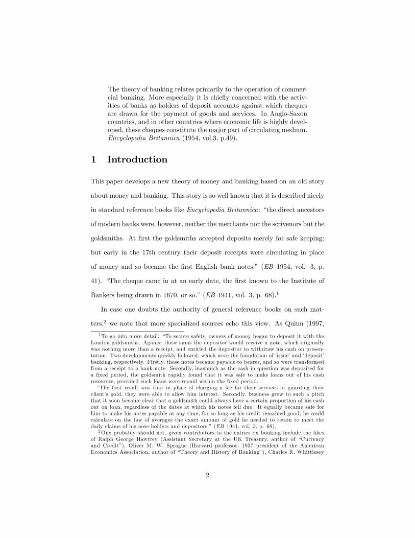
The theory of banking relates primarily to the operation of commer-cial banking. More especially it is chie�y concerned with the activ-ities of banks as holders of deposit accounts against which chequesare drawn for the payment of goods and services. In Anglo-Saxoncountries, and in other countries where economic life is highly devel-oped, these cheques constitute the major part of circulating medium.Encyclopedia Britannica (1954, vol.3, p.49).

1 Introduction

This paper develops a new theory of money and banking based on an old story

about money and banking. This story is so well known that it is described nicely

in standard reference books like Encyclopedia Britannica: �the direct ancestors

of modern banks were, however, neither the merchants nor the scrivenors but the

goldsmiths. At �rst the goldsmiths accepted deposits merely for safe keeping;

but early in the 17th century their deposit receipts were circulating in place

of money and so became the �rst English bank notes.� (EB 1954, vol. 3, p.

41). �The cheque came in at an early date, the �rst known to the Institute of

Bankers being drawn in 1670, or so.�(EB 1941, vol. 3, p. 68).1

In case one doubts the authority of general reference books on such mat-

ters,2 we note that more specialized sources echo this view. As Quinn (1997,

1To go into more detail: �To secure safety, owners of money began to deposit it with theLondon goldsmiths. Against these sums the depositor would receive a note, which originallywas nothing more than a receipt, and entitled the depositor to withdraw his cash on presen-tation. Two developments quickly followed, which were the foundation of �issue�and �deposit�banking, respectively. Firstly, these notes became payable to bearer, and so were transformedfrom a receipt to a bank-note. Secondly, inasmuch as the cash in question was deposited fora �xed period, the goldsmith rapidly found that it was safe to make loans out of his cashresources, provided such loans were repaid within the �xed period.�The �rst result was that in place of charging a fee for their services in guarding their

client�s gold, they were able to allow him interest. Secondly, business grew to such a pitchthat it soon became clear that a goldsmith could always have a certain proportion of his cashout on loan, regardless of the dates at which his notes fell due. It equally became safe forhim to make his notes payable at any time, for so long as his credit remained good, he couldcalculate on the law of averages the exact amount of gold he needed to retain to meet thedaily claims of his note-holders and depositors.� (EB 1941, vol. 3, p. 68).

2One probably should not, given contributors to the entries on banking include the likesof Ralph George Hawtrey (Assistant Secretary at the UK Treasury, author of �Currencyand Credit�), Oliver M. W. Sprague (Harvard professor, 1937 president of the AmericanEconomics Association, author of �Theory and History of Banking�), Charles R. Whittlesey

2

p. 411-12) puts it, �By the restoration of Charles II in 1660, London�s gold-

smiths had emerged as a network of bankers. ... Some were little more than

pawn-brokers while others were full service bankers. The story of their system,

however, builds on the �nancial services goldsmiths o¤ered as fractional reserve,

note-issuing bankers. In the 17th century, notes, orders, and bills (collectively

called demandable debt) acted as media of exchange that spared the costs of

moving, protecting and assaying specie.�Similarly, Joslin (1954, p.168) writes

�the crucial innovations in English banking history seem to have been mainly

the work of the goldsmith bankers in the middle decades of the seventeenth cen-

tury. They accepted deposits both on current and time accounts from merchants

and landowners; they made loans and discounted bills; above all they learnt to

issue promissory notes and made their deposits transferrable by �drawn note�

or cheque; so credit might be created either by note issue or by the creation of

deposits, against which only a proportionate cash reserve was held.�

This is not to suggest that there were no �nancial institutions or intermedi-

aries of interest around other than, or prior to, goldsmith bankers.3 However,

these institutions did not seem to provide anything like circulating demandable

debt, and transferring funds from one account to another �generally required

the presence at the bank of both payer and payee�(Kohn 1999b). That is, �In

(Penn professor, author of �Principles and Practices of Money and Banking�), and EdwardVictor Morgan, (Swansea and Manchester professor, author of �The Theory and Practice ofCentral Banking�).

3Neal (1994) discusses some that were around along with the goldsmith bankers, includingthe scrivenors, merchant banks, country banks, etc. Amongst others, Kohn (1999a,b,c) andDavies (2002) provide extensive discussions of various other institutions in di¤erent placesand times. Particularly well known are the Italian bankers: �To avoid coin for local payments,Renaissance moneychangers had earlier developed deposit banking in Italy, so two merchantscould go to a banker and transfer funds from one account to another.� (Quinn 2002). Goingback further, it seems that the �rst group that might deserve to be called bankers werethe Templars, a religious order of knights during the Crusades. Because they were �erce�ghters, they specialized in moving money around safely. After this they began providingother �nancial services, including loans. They were quite successful for a time � until someof their leadership began loosing their heads in dealings with certain kings. See Weatherford(1977) for more on their fascinating history.

3

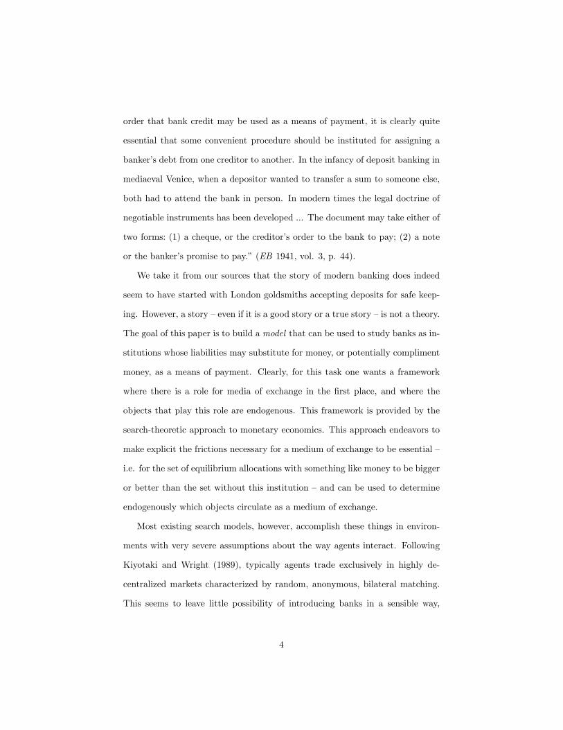
order that bank credit may be used as a means of payment, it is clearly quite

essential that some convenient procedure should be instituted for assigning a

banker�s debt from one creditor to another. In the infancy of deposit banking in

mediaeval Venice, when a depositor wanted to transfer a sum to someone else,

both had to attend the bank in person. In modern times the legal doctrine of

negotiable instruments has been developed ... The document may take either of

two forms: (1) a cheque, or the creditor�s order to the bank to pay; (2) a note

or the banker�s promise to pay.�(EB 1941, vol. 3, p. 44).

We take it from our sources that the story of modern banking does indeed

seem to have started with London goldsmiths accepting deposits for safe keep-

ing. However, a story �even if it is a good story or a true story �is not a theory.

The goal of this paper is to build a model that can be used to study banks as in-

stitutions whose liabilities may substitute for money, or potentially compliment

money, as a means of payment. Clearly, for this task one wants a framework

where there is a role for media of exchange in the �rst place, and where the

objects that play this role are endogenous. This framework is provided by the

search-theoretic approach to monetary economics. This approach endeavors to

make explicit the frictions necessary for a medium of exchange to be essential �

i.e. for the set of equilibrium allocations with something like money to be bigger

or better than the set without this institution �and can be used to determine

endogenously which objects circulate as a medium of exchange.

Most existing search models, however, accomplish these things in environ-

ments with very severe assumptions about the way agents interact. Following

Kiyotaki and Wright (1989), typically agents trade exclusively in highly de-

centralized markets characterized by random, anonymous, bilateral matching.

This seems to leave little possibility of introducing banks in a sensible way,

4

although there have been a few interesting attempts.4 The recent model devel-

oped in Lagos and Wright (2002) deviates from previous analyses by assuming

that agents interact periodically in both decentralized markets and centralized

markets. This was initially used mainly to simplify outcomes in the decentral-

ized market, as under certain assumptions all agents of a given type choose the

same money balances to take out of the centralized and into the decentralized

markets. But once the centralized markets are up and running it is easy to

introduce labor, capital and other markets into this search model in a natural

way (see e.g. Aruoba and Wright 2003).

This framework �ts our needs well. The fact that agents sometimes interact

in highly decentralized markets makes a medium of exchange essential, and we

will determine endogenously whether this ends up being cash, bank liabilities,

or both. The fact that agents sometimes interact in centralized markets allows

us to think about a competitive banking industry where agents make deposits

against which they can make payments, take out loans, etc. The reason agents

may want to use bank deposits instead of cash as a means of payment in the

model is exactly the reason they did in the historical record: safe keeping. That

is, in the model cash will be subject to theft while assets deposited in banks�

vaults will not. There were other problems with money that contributed to the

development of deposit banks and bills of exchange to reduce the need for cash

�among other things, coins were in short supply, were hard to transport, got

clipped or worn, and were not all that easy to recognize or evaluate �but the

4Previous work that incorporates some notion of banks into search models includes Cav-alcanti and Wallace (1999a,b), Cavalcanti et al. (1999), and Williamson (1999). We willnot attempt to review the vast banking literature here, except to mention a few papers thatincorporate banks into models with some microfoundation for money. Analyses in overlap-ping generations models include Williamson (1987), Champ et al. (1996), Schreft and Smith(1998), and Bullard and Smith (2003). Aiyagari and Williamson (2000) and Andolfatto andNosal (2003) provide di¤erent approaches. For an extensive survey of the more conventionalbanking research, most of which is surprisingly far from the microfoundations of money, seeGorton and Winton (2002).

5

modeling the problem as one of safety is natural for our purposes, and leads to

some interesting results.

Of course, formalizing banks as providing a means of payment that is rel-

atively safe � as opposed to, say, relatively easy to transport or to recognize

�means we need to take some care in the way we interpret these assets. A

strict interpretation is that they are checking accounts, or maybe even better,

modern travellers�checks, which are nearly as widely accepted as cash and safer

for at least two reasons: they are less valuable to thieves because they require

a signature that matches the one recorded when making a deposit; and even

if they are lost or stolen you can get your money back at essentially no cost.

This safety aspect of our assets is consistent with the historical view of services

provided by deposit banks, or more generally by bills of exchange which were

not payable to the bearer.5 It is not so clear that our assets are much like bank

notes, which presumably were about as easy to steal as money, and payable

to the bearer. In any case, we think that constructing a formal model of the

endogenous circulation of money and demand deposits seems worthwhile, and

our basic methods should apply to constructing similar models with bank notes

based on some other feature �perhaps recognizability �rather than safety.

Moreover, although checks are less important today than 50 years ago, the

statement in the epigram still applies: checks remain the most common means

5 It may be useful to de�ne some terms. A bill of exchange is an order in writing, signed bythe person giving it (the drawer), requiring the person to whom it is addressed (the drawee)to pay on demand or at some �xed time a given sum of money either to a named person (thepayee) or to the bearer. A cheque is a particular form of bill, where a bank is the draweeand it must be payable on demand. Quinn (2002) also suggests that bills were �similar to amodern traveller�s check.� It is clear that safety was and is a key feature of checks. For onething, the payee needs to endorse the check, so no one else can cash it without committingforgery; other features include the option to �stop�a check or �cross�it (make it payable onlyon presentation by a banker). Indeed, the word �check� or �cheque� originally signi�ed thecounterfoil or indent of an exchequer bill, on which was registered details of the principal partin order to reduce the risk of alteration or forgery. The check or counterfoil parts remainedin the hands of the banker, the portion given to the customer being termed a �drawn note�or �draft.�

6

of payment. �There has been a 20% drop in personal and commercial check-

writing since the mid 1990s, as credit cards, check cards, debit cards, and online

banking services have reduced the need to pay with written checks. [But] Checks

are still king. The latest annual �gures from the Federal Reserve show 30

billion electronic transactions and 40 billion checks processed in the United

States.� Also, �While credit cards reduce the number of checks that need to

be written in retail stores, the credit-card balance still has to be paid every

month. And, at least for now, that is usually done by mail � with a paper

check.�(Philadelphia Inquirer, Feb. 14, 2003, p. A1). So the microfoundations

of M1, cash plus demand deposits, is still relevant. More generally, our focus

is on banks�as providers of payment services, which today is as important as

ever given recent moves towards hopefully safer or more convenient services like

debit cards, electronic money, etc.

The rest of the paper and our main results can be summarized as follows.

The analysis is organized around a sequence of formal models, each adding an

additional component. Section 2 presents the basic assumptions which make a

medium of exchange essential, and which allow this role to be �lled by money or

checks. Section 3 analyzes the simplest case, where theft is exogenous, money

and goods are indivisible, and we have 100% reserve requirements. With no

banking, this model is a simple extension of the textbook search-based model of

monetary exchange. Once banks are added, we show there can exist equilibria

where all agents, no agents, or some agents use checks, and sometimes these

equilibria coexist. An interesting result is that sometimes monetary equilibria

do not exist without banks but do exist with banks, so in a sense money and

banking are complimentary. We also show how the equilibrium set changes as

parameters like the cost of banking or the supply of outside money change.

7

Section 4 endogenizes theft. Without banks, this provides a slightly more

interesting extension of the textbook search model, and generates some sim-

ple but intuitively reasonable results: e.g. equilibria with theft are more likely

when production is more costly; too much theft is inconsistent with monetary

equilibrium; and sometimes there are multiple equilibria with di¤erent amounts

of theft. When we introduce banks we again expand the set of parameters for

which monetary equilibria exist, so again money and banking are complimen-

tary, but now there are two reasons: as in the model with exogenous theft, the

safety provided by banks makes money more valuable, but now there is an ad-

ditional e¤ect because when fewer people carry cash the number of thieves may

fall. An interesting result in the model with endogenous theft is that checks

can never completely drive out money. The reason is that if no one carries cash

there are no thieves, but then you may as well use cash. Hence, concurrent

circulation of money and bank liabilities is a natural outcome.

Section 5 generalizes the model to allow divisible goods and shows the basic

results are robust.6 Section 6 relaxes the 100% reserve requirement by allowing

banks to lend a certain fraction of their deposits. The loan rate is determined

by supply and demand in the centralized market. One feature of this model

is that the fee charged for checking service will be less than the resource cost

of managing the account, since banks pro�t from making loans, and as with

the goldsmiths they may end up charging a negative fee (i.e. paying interest

on demand deposits). In this case, checks could possibly drive cash out of

6Although we allow divisible goods in this section, we retain the assumption of indivis-ible money and a unit upper bound on asset holdings throughout the paper. Thus, we donot exploit one of the main advantages of the Lagos-Wright structure � that under certainassumptions on preferences, it allows one to dispense with indivisible assets and the upperbound with a minimal loss in tractability. The only feature of the framework that we reallyuse here is that agents have periodic access to centralized markets, where they can do theirbanking, and also periodically interact in highly decentralized markets so that some mediumof exchange is essential. We wanted to explore the simplest indivisible asset models �rst; fullydivisible asset models are being explored in a follow-up paper.

8

circulation. This version of the model also generates a simple money multiplier,

as in undergraduate textbooks, although here the role of money and banks are

explicitly modeled from microeconomic principles. Section 7 concludes.

2 Basic Assumptions

The economy is populated by a [0; 1] continuum of in�nitely-lived agents. Time

is discrete, continues forever. Following Lagos and Wright (2002), each period

is divided into two subperiods, say day and night. During the day agents will

interact in a centralized (frictionless) market, while at night they will interact

in a highly decentralized market characterized by random, anonymous, bilateral

matching. Trade is di¢ cult in the decentralized markets because of a standard

double coincidence problem: there are many specialized goods traded in this

market, and only a fraction x 2 (0; 1) of the population can produce a spe-

cialized good that you want. A meeting where someone can produce what you

want is called a single coincidence meeting; for simplicity, there are no double

coincidence meetings so that we can ignore pure barter, but it is easy to relax

this. As they are nonstorable, these goods are produced for immediate trade

and consumption. Goods are also indivisible for now, but this is relaxed below.

Consuming a specialized good that you want conveys utility u. Producing a

specialized good for someone else conveys disutility c < u. The rate of time

preference is r > 0.

Due to the frictions in the decentralized market, trade would shut down

if not for a medium of exchange; in particular, since agents are anonymous

there can be no credit (Kocherlakota 1998; Wallace 2001). Hence, a fraction

M 2 [0; 1] of the population are each initially endowed with one unit of money

�an object that is consumed or produced by no one, but may have potential

9

use as a means of payment. For simplicity, if not historical accuracy, one can

think if this money as �at, although it would be easy to redo things in terms of

commodity money (say, following Velde et al. 1999). Here we follow the early

literature in the area and assume that money is indivisible and agents can store

at most one unit at a time. A key feature of the model is that this money is

unsafe �it can be stolen. We assume for simplicity that goods cannot be stolen.

Also, because individuals can store at most one unit of money, only individuals

without money steal.

We formalize stealing as follows.7 In the decentralized market, if you meet

an agent holding cash you attempt to steal it with probability �, which is en-

dogenous in some versions of the model studied below and exogenous in others

(you just can�t help it). Given that you try to steal, with probability you

are successful. Theft has a cost z < u. Note that theft may be more or less

costly than honest trade, depending on z � c, and also may be more or less

likely to succeed, depending on � x. Agents in the day subperiod can deposit

their money into a bank, and can write checks on these accounts. Checks are

assumed to be perfectly safe. Also, all agents believe a bank can be counted

on to cash a check as long as it has been signed by the depositor.8 This means

that everyone is as willing to accept a check in the decentralized night market

as cash, since they know the former can be turned into the latter in the next

day�s centralized market.

In terms of the centralized day market, we make it as simple as possible to

7Criminal activity here is pretty simple, even when � is endogenous, but can be thoughtof as following the search-theoretic models of crime in Burdett et al. (2003) and Huang et al.(2004). There is also a sense in which the present model seems closely related to the analysis ofmonetary exchange under private information in Williamson and Wright (1994), since stealingyour money is conceptually not very di¤erent from selling you low quality merchandise. Thatpaper did not have anything like banks, however.

8This belief is assumed exogenously here, say because there is a legal enforcement mecha-nism at work, but it should not be hard to use reputation to get banks to honor their debtsendogeneously.

10

focus on decentralized trade. First, we assume that di¤erent goods are produced

during the day and night �during the day agents cannot produce the specialized

goods traded at night, but rather some general good. Consuming Q units of

this general good conveys utility Q and producing Q units conveys disutility

�Q. This can be relaxed without much di¢ culty but it eases the presentation

slightly since it implies that agents would never trade general goods for their

own sake; their only role will be to settle interest or fees with banks. General

goods are perfectly divisible, but they are nonstorable so they cannot be used

to trade for special goods in the decentralized market. Claims to future general

goods also cannot be used in the decentralized market, unless these are claims

drawn on a bank. That is, personal IOU�s cannot be used in payment, but

checks can.

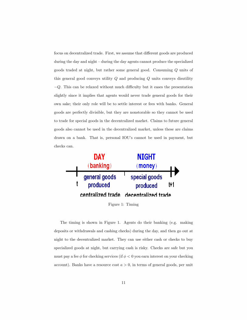
Figure 1: Timing

The timing is shown in Figure 1. Agents do their banking (e.g. making

deposits or withdrawals and cashing checks) during the day, and then go out at

night to the decentralized market. They can use either cash or checks to buy

specialized goods at night, but carrying cash is risky. Checks are safe but you

must pay a fee � for checking services (if � < 0 you earn interest on your checking

account). Banks have a resource cost a > 0, in terms of general goods, per unit

11

of money on deposit. Also, in general they are required legally to keep a fraction

� of their deposits on reserve, while the rest can be loaned out. Loans may be

demanded by some of the 1�M agents who begin the day without purchasing

power. We assume competitive banking, so the cost of a loans � will equate the

supply and demand for loans. Thus, for example, if � = 1 banks must keep all

cash deposits in the vault, in which case competition implies � = a.

3 Exogenous Theft

In this section we study the model where stealing is exogenous: if an agent with

money meets one without, the latter will try to rob the former with some �xed

probability �. With probability he succeeds, while with probability 1� he

fails and walks away empty handed. We �rst study the case where the only

asset is money and then we introduce banking. We also assume 100% reserve

requirements for now: � = 1.

3.1 Money

Throughout the paper we use V1 to represent the value function of an agent with

1 unit of money, called a buyer, and V0 the value function of an agent with no

money, called a seller. When there are no banks, Figure 2 shows the event trees

for buyers and sellers in the night market. For example, a buyer with probability

M meets another buyer and he leaves as a buyer; with probability 1 �M he

meets a seller, and in this case with probability � the seller tries to rob him and

succeeds with probability , while with probability 1� � they try to trade and

succeed with probability x. The �ow Bellman equations corresponding to these

12

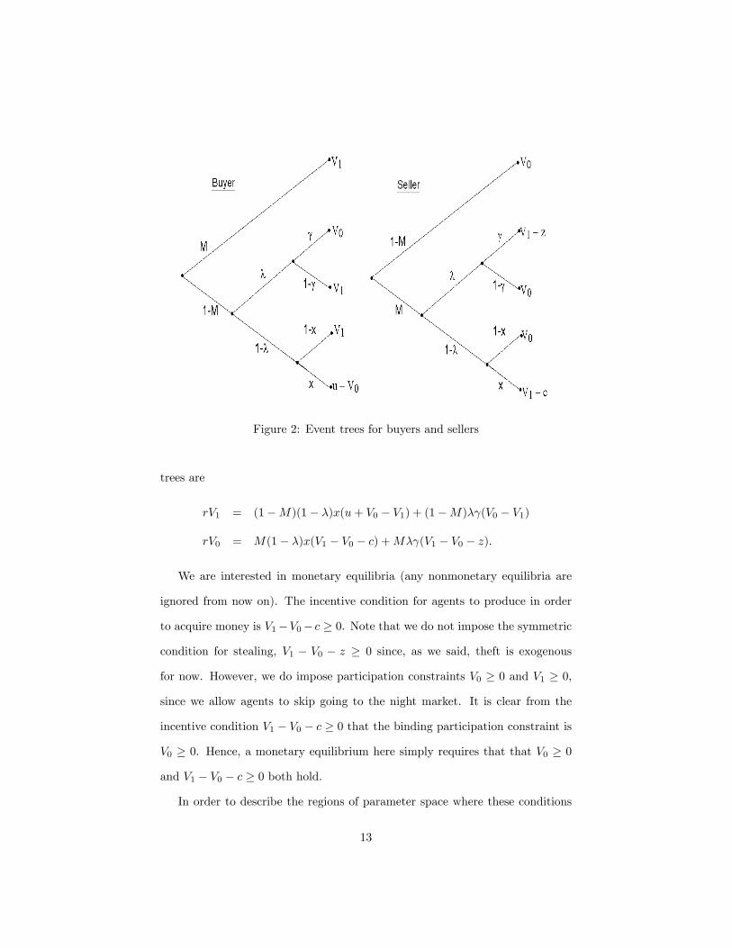
Figure 2: Event trees for buyers and sellers

trees are

rV1 = (1�M)(1� �)x(u+ V0 � V1) + (1�M)� (V0 � V1)

rV0 = M(1� �)x(V1 � V0 � c) +M� (V1 � V0 � z):

We are interested in monetary equilibria (any nonmonetary equilibria are

ignored from now on). The incentive condition for agents to produce in order

to acquire money is V1�V0� c � 0. Note that we do not impose the symmetric

condition for stealing, V1 � V0 � z � 0 since, as we said, theft is exogenous

for now. However, we do impose participation constraints V0 � 0 and V1 � 0,

since we allow agents to skip going to the night market. It is clear from the

incentive condition V1 � V0 � c � 0 that the binding participation constraint is

V0 � 0. Hence, a monetary equilibrium here simply requires that that V0 � 0

and V1 � V0 � c � 0 both hold.

In order to describe the regions of parameter space where these conditions

13

hold, and hence where a monetary equilibrium exists, de�ne

CM =(1�M)(1� �)xu+M� zr + (1�M)(1� �)x+ �

CA =(1�M)[� + (1� �)x]ur + (1�M)[� + (1� �)x] �

� z

(1� �)x:

Figure 3 depicts CM and CA in (x; c) space using properties in the following

easily veri�ed Lemma.

Figure 3: Existence region for monetary equilibrium

Lemma 1 (a) x = 0 ) CM = M� zr+� , CA = �1. (b) C 0M > 0, C 0A > 0. (c)

CM = CA i¤ (x; c) = (x�; z), where x� =[r+(1�M)� ]z

(1�M)(1��)(u�z) .

We can now verify the following.

Proposition 1 Monetary equilibrium exists i¤ c � minfCM ; CAg.

Proof: Subtracting the Bellman equations and rearranging implies

V1 � V0 =(1� �)x[(1�M)u+Mc] + � Mz

r + (1� �)x+ � :

Algebra implies V1 � V0 � c � 0 i¤ c � CM and V0 � 0 i¤ c � CA. �

14

Naturally, monetary equilibrium is more likely to exist when c is lower or x

bigger.9 Also notice that either of the two constraints c � CM and c � CA may

bind. It is easy to see that welfare, as measured by average utility

W =MV1 + (1�M)V0 =M(1�M)

r[(1� �)x(u� c)� � z] ;

is decreasing in � and . The welfare cost of crime here is due to the resource cost

z and the opportunity cost of thieves not producing; stealing per se is a transfer

not an ine¢ ciency. In any case, when � = 0, so that CM = CA =(1�M)xur+(1�M)x ,

we essentially have the simple textbook search model of monetary exchange in

Kiyotaki and Wright (1993). Allowing money to be subject to theft provides an

simple but not unreasonable extension of the basic framework. We next show

it can be used to discuss banks.

3.2 Banking

We now allow agents with money to deposit it in checking accounts. Since � = 1

in this section, banks like the early goldsmiths simply keep the money in the

vault and earn revenue by charging � = a for this service, paid in the model in

terms of general goods. Let � be the probability an agent with money decides

each day to put his money in the bank (or, if he already has an account, to not

withdraw it). Let M0 =M(1��) denote the amount of cash in circulation, and

letM1 =M0+M� =M denote cash plus demand deposits. Let Vm be the value

function of an agent in the night market with cash, and Vd the value function of

an agent at night with money deposited in his bank, exclusive of the fee a. Hence,

for an agent with 1 dollar in the centralized market, V1 = maxfVm; Vd � ag.9One might also expect @CM=@� < 0, but actually this is true i¤ z < ~z =

(1�M)(r+ )xuM [r+(1�M)x)]

;thus, for large z, when � increases agents are more willing to acept money. This is because� measures not only the probability of being robbed but also the probability of trying to robsomeone else; when z is very big, if this probability goes up agents are more willing to workfor money to keep themselves from crime. This e¤ect may seem strange, but in any case itgoes away when � is endogenized.

15

Although checks will be perfectly safe, it facilitates the discussion to tem-

porarily proceed more generally and let m and d be the probabilities that one

can successfully steal from someone with money and from someone with a bank

account. Bellman�s equation for an agent with asset j 2 fm; dg is then10

rVj = (1�M)(1� �)x(u+ V0 � V1) + (1�M)� j(V0 � V1) + V1 � Vj :

For an agent without money

rV0 = (1� �)Mx(V1 � V0 � c) + � [M0 m + (M �M0) d] (V1 � V0 � z):

If we set m = and d = 0, then

rVm = (1�M)(1� �)x(u+ V0 � V1) + (1�M)� (V0 � V1) + V1 � Vm

rVd = (1�M)(1� �)x(u+ V0 � V1) + V1 � Vd

rV0 = (1� �)Mx(V1 � V0 � c) + �M0 (V1 � V0 � z):

We also have V1 = maxfVm; Vd � ag = �(Vd � a) + (1� �)Vm, from which it

is clear that

� = 1) Vd � a � Vm; � = 0) Vd � a � Vm; and � 2 (0; 1)) Vd � a = Vm:

Equilibrium satis�es this condition, plus the incentive condition for money to

be accepted, V1 � V0 � c � 0, and the participation condition, V0 � 0. To

characterize the parameters for which di¤erent types of equilibria exist, de�ne

C1 = � (1�M)uM

� � z

(1� �)x +[r + (1� �)x+ � ]aM(1�M)�(1� �) x

C2 =(1�M)(1� �)xu� ar + (1�M)(1� �)x

C3 = � (1�M)uM

+[r + (1� �)x+ (1�M)� ]aM(1�M)�(1� �) x

10The value of entering the decentralized market with asset j is

Vj =1

1 + r[(1�M)(1� �)x(u+ V0) + (1�M)� jV0 + �V1]

where � = 1� (1�M)(1� �)x� (1�M)� j . Multiplying by 1 + r and subtracting Vj fromboth sides yields the equation in the text.

16

where a = (1 + r)a.

Figure 4 show the situation in (x; c) space for the two possible cases, z < C4

and z > C4, where

C4 =a

(1�M)� :

We assume C4 < u, or a < (1 � M)� u, to make things interesting. The

following Lemma establishes that the Figures are drawn correctly by describing

the relevant properties of Cj , and relating them to CM and CA from the case

with no banks; again the easy proof is omitted.

Figure 4: Conditions in Lemma 2

Lemma 2 (a) x = 0) C1 =1 or �1, C2 = �a=r < 0, C3 =1. (b) C 02 > 0,

C 03 < 0, and C1 is monotone but can be increasing or decreasing. (c) C1 = CM

i¤ (x; c) = (�x;C4), C2 = C3 i¤ (x; c) = (~x;C4), and C1 = CA i¤ (x; c) = (~x; ~C),

where

�x =a(r + � )�M(1�M)�2 2z

(1�M)(1� �)[(1�M)� u� a]

~x =a[r + (1�M)� ]

(1�M)(1� �)[(1�M)� u� a] :

(d) �x > ~x i¤ z < C4 < ~C and �x < ~x i¤ z > C4 > ~C.

17

We can now prove the following:

Proposition 2 (a) � = 0 is an equilibrium i¤ c � min(CM ; CA; C1). (b) � = 1

is an equilibrium i¤ C3 � c � C2. (c) � 2 (0; 1) is an equilibria i¤ either:

z < C4, c 2 [C3; C1] and c � C4; or z > C4, c 2 [C1; C3] and x � ~x.

Proof: Consider � = 0, which implies M1 =M0 =M and V1 = Vm. For this

to be an equilibrium we require Vm�V0�c � 0 and V0 � 0, which is true under

exactly the same conditions as in the model with no banks, c � min(CM ; CA).

However, now we also need to check Vm � Vd � a so that not going to the

bank is an equilibrium strategy. This holds i¤ c � C1. Now consider � = 1,

which implies M0 = 0 and V1 = Vd � a. In this case, V1 � V0 � c � 0 holds i¤

c � C2. We also need V0 � 0, but this never binds. Finally, we need to check

Vd � a � Vm, which is true i¤ c � C3.

Finally consider � 2 (0; 1), which implies M0 = M(1 � �) 2 (0;M) is en-

dogenous and V1 = Vd � a = Vm. The Bellman equations imply

(1 + r)(Vd � Vm) = (1�M)� (V1 � V0):

Inserting Vd � Vm = a and

V1 � V0 =(1� �)x[(1�M)u+Mc] +M0� z

r + (1� �)x+ (1�M +M0)� ;

we can solve for

M0 =(1�M)�(1��) x[(1�M)u+Mc]�[r+(1��)x+(1�M)� ]a

(C4�z)(1�M)�2 2:

We need to check M0 2 (0;M), which is equivalent to � 2 (0; 1). There are two

cases, depending on the sign of the denominator: if z < C4 then M0 2 (0;M)

i¤ c 2 (C3; C1), and if z > C4 then M0 2 (0;M) i¤ c 2 (C1; C3). We also need

to check V1 � V0 � c � 0, which holds i¤ c � C4, and V0 � 0, which holds i¤

18

x � ~x. When �x > ~x the binding constraint is c � C4, and when �x < ~x the

binding constraint is x � ~x. �

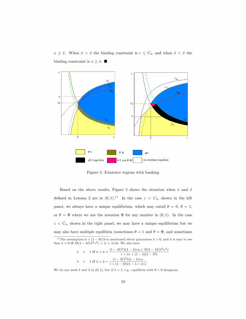
Figure 5: Existence regions with banking

Based on the above results, Figure 5 shows the situation when �x and ~x

de�ned in Lemma 2 are in (0; 1).11 In the case z > C4, shown in the left

panel, we always have a unique equilibrium, which may entail � = 0, � = 1,

or � = � where we use the notation � for any number in (0; 1). In the case

z < C4, shown in the right panel, we may have a unique equilibrium but we

may also have multiple equilibria (sometimes � = 1 and � = �, and sometimes

11The assumption a < (1�M)� u mentioned above guarantees ~x > 0, and it is easy to seethat �x > 0 i¤M(1�M)�2 2z < (r + � )a. We also have

�x < 1 i¤ a < �a =(1�M)2�(1� �) u+M(1�M)�2 2z

r + � + (1� �)(1�M)

~x < 1 i¤ a < ~a =(1�M)2�(1� �) u

r + (1�M)(1� �+ � ):

We do not need �x and ~x in (0; 1), but if ~x > 1, e.g., equilibria with � > 0 disappear.

19

all three equilibria). Recall that without banks the monetary equilibrium exists

i¤ c � minfCM ; CAg. Hence, if it exists without banks monetary equilibrium

still exists with banks, and it may or may not entail � > 0. However, there are

parameters such that there are no monetary equilibria without banks while there

are with banks. In these equilibria we must have � > 0, although not necessarily

� = 1. The important economic point is that for some parameters, and in

particular for relatively large x and c, money cannot work without banking but

it can work with it.

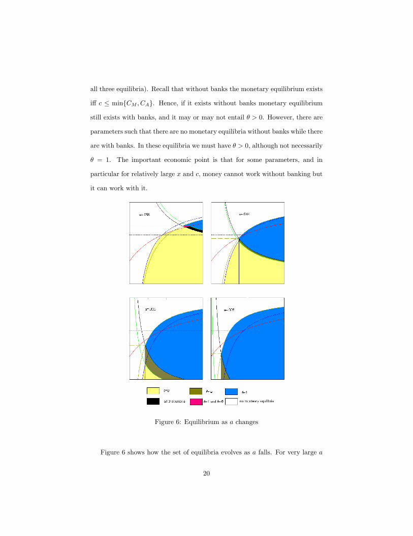
Figure 6: Equilibrium as a changes

Figure 6 shows how the set of equilibria evolves as a falls. For very large a

20

banking is not viable, so the only equilibrium is � = 0. As we reduce a two things

happen: in the some regions where there was a monetary equilibrium without

banks, agents may start using banks; and in some regions where there were no

monetary equilibria without banks, a monetary equilibrium emerges. As a falls

further the region where � = 0 shrinks. As a falls still further we switch from

the case z < C4 to the case z > C4; thus, for relatively small a equilibrium must

be unique, but could entail � = 1, � = 0, or � = �. As a falls even further, we

lose equilibrium with � = 0. Eventually checks drive currency from circulation.

Note however that this is not robust: in the next section we endogenize � and

show that banking never completely drives out money. Equilibria with � 2 (0; 1)

are particularly interesting because they yield the concurrent circulation of cash

and checks.

A similar picture emerges if we let M fall, since reducing M also raises the

demand for checking services. One arguably strange reason for this is that in

the present model lower M implies a greater number of criminals (1 �M)�.

However, we can circumvent this by considering what happens as we vary M

and adjust � to keep (1 � M)� constant. Lower M still makes � > 0 more

likely, but now the reason is simply that lower M makes money more valuable,

so you are willing to pay more to keep it safe. See Figure 7, where the two

rows are for Z < C4 and Z > C4, and in either case M falls as we move from

left to right. The result that lower M makes it more likely that agents will use

banking is consistent with the historical evidence that people were more likely

to use demandable debt as a means of payment when cash was in short supply

(Ashton 1945; Cuadras-Morato and Rosés 1998), although one can presumably

tell a variety of stories consistent with this. In any case, although the model is

simple, we think it captures something interesting about banking.

21

Figure 7: Equilibrium as M changes

4 Endogenous Theft

In this section we endogenize the decision to be a thief. This is useful not

only for the sake of generality, but because the model with � exogenous does

have some features one may wish to avoid (e.g. when M goes down the crime

rate mechanically increases). Moreover, an interesting implication of the model

with � endogenous is that checks can never completely drive currency from

circulation: if no one uses cash, no one will choose crime, but then cash is safe

22

and no one would use checks. Hence concurrent circulation is more likely. As

in the model with exogenous �, we start with the case where money is the only

asset and then introduce banks.

4.1 Money

Let � now be the probability an individual without money chooses to be a thief

before going out at night. Bellman�s equation for V1 is the same as in Section

3.1. Bellman�s equations for producers and thieves are now

rVp = Mx(V1 � Vp � c) + (1�Mx)(V0 � Vp)

rVt = M (V1 � Vt � z) + (1�M )(V0 � Vt);

where V0 = maxfVt; Vpg = �Vt + (1� �)Vp. The equilibrium conditions are

� = 1) Vt � Vp, � = 0) Vt � Vp, and � 2 (0; 1)) Vt = Vp;

plus the incentive condition V1 � V0 � c � 0. Notice that with � endogenous

we do not have to check the participation constraint V0 � 0: since an agent can

always set � = 0, we have rV0 � Mx(V1 � V0 � c) � 0 as long as the incentive

condition holds.

The next observation is that we can never have equilibrium with � = 1,

since we cannot have agents accepting money when everyone is a thief.12 To

say more, de�ne the following thresholds

c0 =(1�M)xur + (1�M)x

c1 =(x� )(1�M)xu+ (r + x)z

x[r + (1�M)x+M ]

c2 =[r +Mx+ (1�M) ] z

(r + )x:

12Formally, if V1 � V0 � c � 0 then � = 1) rV1 = (1�M) (V0 � V1) � �(1�M)� c < 0,and therefore V1 � V0 � c < 0. Hence, � < 1 in any equilibrium.

23

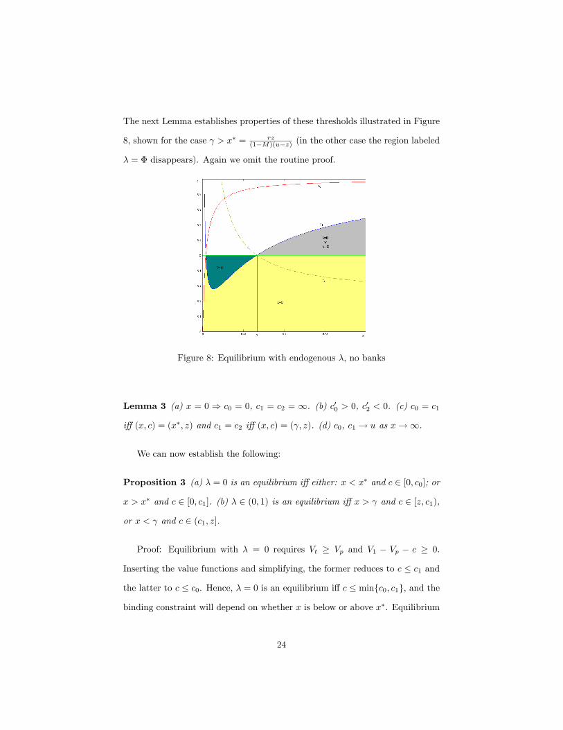
The next Lemma establishes properties of these thresholds illustrated in Figure

8, shown for the case > x� = rz(1�M)(u�z) (in the other case the region labeled

� = � disappears). Again we omit the routine proof.

Figure 8: Equilibrium with endogenous �, no banks

Lemma 3 (a) x = 0 ) c0 = 0, c1 = c2 = 1. (b) c00 > 0, c02 < 0. (c) c0 = c1

i¤ (x; c) = (x�; z) and c1 = c2 i¤ (x; c) = ( ; z). (d) c0, c1 ! u as x!1.

We can now establish the following:

Proposition 3 (a) � = 0 is an equilibrium i¤ either: x < x� and c 2 [0; c0]; or

x > x� and c 2 [0; c1]. (b) � 2 (0; 1) is an equilibrium i¤ x > and c 2 [z; c1),

or x < and c 2 (c1; z].

Proof: Equilibrium with � = 0 requires Vt � Vp and V1 � Vp � c � 0.

Inserting the value functions and simplifying, the former reduces to c � c1 and

the latter to c � c0. Hence, � = 0 is an equilibrium i¤ c � minfc0; c1g, and the

binding constraint will depend on whether x is below or above x�. Equilibrium

24

with � 2 (0; 1) requires Vt = Vp and V1 � V0 � c � 0. We can solve Vt = Vp for

� = ��, where

�� =( � x)x[(1�M)u+Mc]� (r + x)( z � xc)

( � x)(1�M)(xu� xc+ z) :

It can be checked that �� 2 (0; 1) i¤ c 2 (c1; c2) when x < and �� 2 (0; 1)

i¤ c 2 (c2; c1) when x > . The condition V1 � V0 � c � 0 can be seen to hold

i¤ c � z when x < and i¤ c � z when x > . Hence, � = �� 2 (0; 1) is an

equilibrium i¤ c 2 (c1; z] when x < , and i¤ c 2 [z; c1) when x > . �

As seen in the �gure, a monetary equilibrium is again more likely to exist

when c is low or x is high. Given a monetary equilibrium exists, it is more

likely that � = 0 when c is low or x is high, since both of these make honest

production relatively attractive. Given x, it is more likely that � 2 (0; 1) when

c is bigger. When x� < , there is a region of (x; c) space with x < where

an equilibrium with � 2 (0; 1) exists and is unique. Regardless of x�, as long

as c0 > z at x = 1, there exists a region where equilibrium with � 2 (0; 1)

and � = 0 coexist. A very interesting aspect of the results is the following.

In constructing equilibrium with � 2 (0; 1) we need to guarantee � < 1, but

this is actually never binding: as � increases we hit the incentive constraint for

money to be accepted before we reach � = 1. For example, in the region where

� 2 (0; 1) exists uniquely, as c increases we get more thieves, but before the

entire population resorts to crime people stop producing in exchange for cash

and money stops circulating.

25

4.2 Banking

Bellman�s equations are

rVm = (1�M)(1� �)x(u+ V0 � V1) + (1�M)� (V0 � V1) + V1 � Vm

rVd = (1�M)(1� �)x(u+ V0 � V1) + V1 � Vd

rVp = Mx(V1 � Vp � c) + (1�Mx)(V0 � Vp)

rVt = M0 (V1 � Vt � z) + (1�M0 )(V0 � Vt);

where V1 = maxfVm; Vd � ag and V0 = maxfVp; Vtg. Equilibrium requires the

choice of crime to satisfy

� = 1) Vt � Vp; � = 0) Vt � Vp; and � 2 (0; 1)) Vt = Vp;

and the choice of going to the bank satisfy

� = 1) Vd � a � Vm; � = 0) Vd � a � Vm; and � 2 (0; 1)) Vd � a = Vm:

In this section, since things are more complicated, we analyze possible equi-

libria one at a time. In principle there are nine qualitatively di¤erent types of

equilibria, since each endogenous variable � and � can be 0, 1, or � 2 (0; 1), but

we can quickly rule out all but three possibilities.

Lemma 4 The only possible equilibria are: � = 0 and � = 0; � = 0 and

� 2 (0; 1); and � 2 (0; 1) and � 2 (0; 1).

Proof: Clearly � = 1 cannot be an equilibrium, as then no one accepts

money. If � = 0 then there are no thieves, so money is safe and � = 0. Finally,

if � = 1 then Vt = 0 and so we cannot have � > 0. �

Proposition 4 � = 0 and � = 0 is an equilibrium i¤ either: x < x� and

c 2 [0; c0]; or x > x� and c 2 [0; c1].

26

Proof: Given � = 0, it is clear that � = 0 is a best response. Hence the only

conditions we need are V1 � V0 � c � 0 and Vp � Vt. With � = 0 these are

equivalent to the conditions from the model with no banks. �

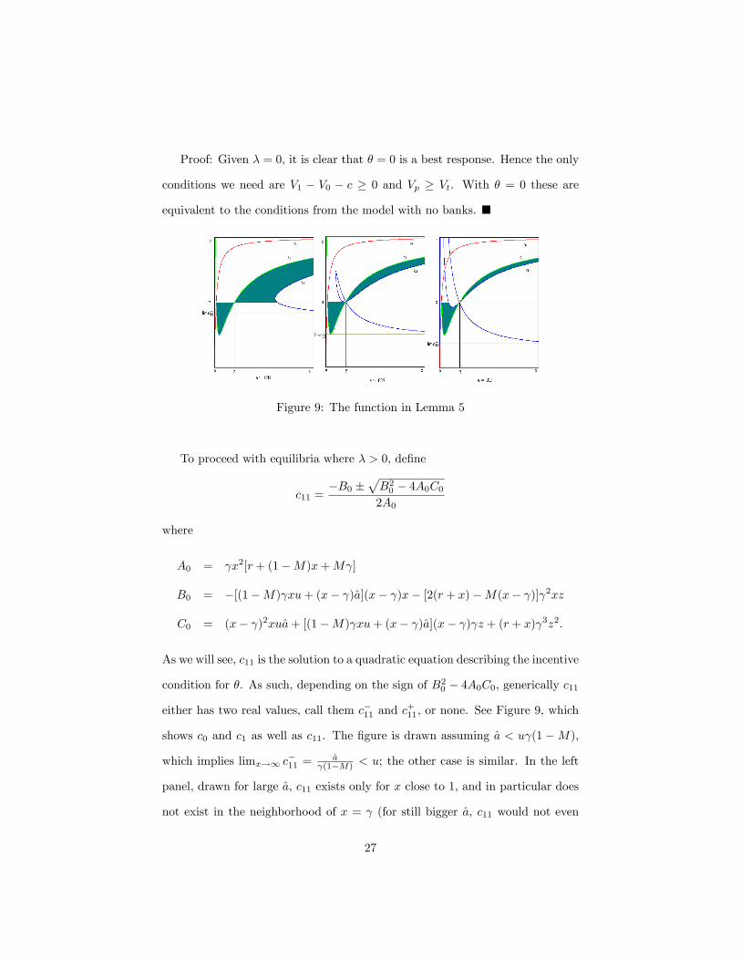
Figure 9: The function in Lemma 5

To proceed with equilibria where � > 0, de�ne

c11 =�B0 �

pB20 � 4A0C02A0

where

A0 = x2[r + (1�M)x+M ]

B0 = �[(1�M) xu+ (x� )a](x� )x� [2(r + x)�M(x� )] 2xz

C0 = (x� )2xua+ [(1�M) xu+ (x� )a](x� ) z + (r + x) 3z2:

As we will see, c11 is the solution to a quadratic equation describing the incentive

condition for �. As such, depending on the sign of B20 � 4A0C0, generically c11

either has two real values, call them c�11 and c+11, or none. See Figure 9, which

shows c0 and c1 as well as c11. The �gure is drawn assuming a < u (1 �M),

which implies limx!1 c�11 =

a (1�M) < u; the other case is similar. In the left

panel, drawn for large a, c11 exists only for x close to 1, and in particular does

not exist in the neighborhood of x = (for still bigger a, c11 would not even

27

appear in the �gure). As a shrinks, c11 exists for more values of x, and at some

point it exists for x in the neighborhood of , as in the middle panel; notice

c�11 and c+11 happen to coalesce at x = . As a shrinks further, c11 exists for all

x > 0, as in the right panel. One can show the following.

Lemma 5 (a) For x > , if c11 exists then c+11 < c1; for x < , if c11 exists

then c1 < c�11; if c11 exists in the neighborhood of x = then c11 = c1 at

(x; c) = ( ; z). (b) For x > , c+11 ! c1 as a! 0; for x < , c�11 ! c1 as a! 0.

Proposition 5 � = 0 and � 2 (0; 1) is an equilibrium i¤ either: x > , c 2

[z; c1), and c =2 (c�11; c+11); or x < , c 2 (c1; z], and c =2 (c�11; c+11).

Proof: In this case the conditions for � 2 (0; 1) are exactly the same as in the

model without banks, but we now have to additionally check Vm�Vd+a � 0 to

guarantee � = 0. Algebra implies this condition holds i¤ A0c2 +B0c+ C0 � 0,

which is equivalent to c =2 (c�11; c+11). �

The region where equilibrium with � = 0 and � 2 (0; 1) exists is shown

by the shaded area in Figure 9. The economics is simple: in addition to the

conditions for � 2 (0; 1) from the model with no banks, we also have to be sure

now that people are happy carrying cash instead of checks, which reduces to

c =2 (c�11; c+11). For large a this is not much of a constraint. As a gets smaller we

eliminate more of the region where � 2 (0; 1) is an equilibrium. When a ! 0

the relevant branch of c11 converges to c1, and this equilibrium vanishes.

Now consider equilibria with � 2 (0; 1) and � 2 (0; 1). To begin, we have the

following result.

Lemma 6 If there exists an equilibrium with � 2 (0; 1) and � 2 (0; 1), then

� =�B �

pB2 � 4AC

2A(1�M) and � = 1� x[a� (1�M)� c] [a� (1�M)� z]

where A = xu, B = �[(1�M) xu+M xc+ (x� )a], and C = (r + x)a.

28

Proof: In this equilibrium we have V1 = Vm = Vd � a and V0 = Vp =

Vt. Solving Bellman�s equations and inserting the value functions into these

conditions gives us two equations in � and �. One is a quadratic that can be

solved for � = �B�pB2�4AC

2A(1�M) . The other gives us � as a function of the solution

for �. �

In order to reduce the number of possibilities, we concentrate on the smaller

root for � in Lemma 6.13 To see when such an equilibrium exists, de�ne

c3 =�k +

p4(r + x) xua

M x

c4 =�(1�M)2 xu+ [2(r + x)� (x� )(1�M)]a

(1�M)M x

c5 =[r +Mx+ (1�M) ]a

(1�M)M x

c6 =k

[2(r + x)�Mx]

c7 =k+�pk2 � 4[r + (1�M)x] xua2[r + (1�M)x]

c8 =�k + 2(r + x) z

Mx

c9 =xua� kz + (r + x) z2

M xz

c10 =(x� )k + 2(r + x) 2z[2(r + x)�M(x� )]x

where we let k = (1�M) xu+(x� )a to reduce notation. We now prove some

properties of the cj�s and relate them to c0, c1 and c11, continuing to assume

a < (1�M)u.

Lemma 7 (a) x = 0 ) c3 = c4 = c5 = c8 = c9 = c10 = 1 and c6 = � a2r < 0.

(b) c03 < 0, c04 < 0, c05 < 0, c06 > 0, c08 < 0, c09 < 0. (c) c7 � 0 exists i¤

x � x7 2 (0; 1); if c7 exists then c�07 < 0, c+07 > 0 and (c+7 ; c�7 ) !

�a

(1�M) ; u�

as x ! 1; c7 2 (c3; c0) and (c+7 ; c

�7 ) ! (c0; 0) as a ! 0. (d) c10 = c1 at

13 In examples we found it was not impossible to have an equilibrium with � given by thelarger root, but only for a very small set of parameters.

29

(x; c) = ( ; z); c6, c8 and c10 all cross at c = z, and c7, c9 and c11 all cross

at c = z, although the values of x at which these crossing occur need not be in

(0; 1). (e) c3 = c6 = c7 at a point where c7 is tangent to c3; c3 = c10 = c11 at a

point where c11 is tangent to c3.

The cj are shown in (x; c) space in Figure 10 for various values of a progres-

sively decreasing to 0. The shaded area is the region where equilibrium with

� 2 (0; 1) and � 2 (0; 1) exist, as proved in the next Proposition.

Figure 10: Proposition 6 equilibria

Proposition 6 � 2 (0; 1) and � 2 (0; 1) is an equilibrium i¤ all of the following

conditions are satis�ed: (i) c > c� = maxfc3;minfc4; c5gg; (ii) c > maxfc8; c9g

and either c < c6 or c 2 (c�7 ; c+7 ); and either (iii-a) x > , c > maxfz; c10g, and

c =2 (c�11; c+11), or (iii-b) x < and either c > c10 or c 2 (c�11; c+11).

Proof: The previous lemma gives us � as a solution to a quadratic equation

30

and � as a function of �, assuming that an equilibrium with � 2 (0; 1) and

� 2 (0; 1) exists. We now check the following conditions: when does a solution

to this quadratic in � exist; when is that solution in (0; 1); when is the implied

� in (0; 1); and when is V1 � V0 � c.

First, a real solution for � exists i¤ B2 � 4AC � 0, which holds i¤ either of

the following hold:

c � �[(1�M) xu+ (x� )(1 + r)a] +p4(r + x)(1 + r) xua

M x= c3

c � �[(1�M) xu+ (x� )(1 + r)a]�p4(r + x)(1 + r)a xua

M x= c03

Second, given that it exists, � > 0 i¤ B < 0 i¤

c >�(1�M) xu� (x� )(1 + r)a

M x= c003 .

It is easy to check that c3 > c003 > c03, and so � > 0 exists i¤ c � c3.

It will be convenient to let W = V1 � V0. Subtracting the �rst two Bellman

equations, we have Vm � Vd = (1�M)� 1+r W , and hence by the equilibrium condi-

tion for � 2 (0; 1), Vm � Vd = �a, we have ! = a�(1�M) =

�B+pB2�4AC

2(r+x) after

inserting �. We can now see that � < 1 is equivalent to ! > a(1�M) . Analysis

shows this holds i¤ c > minfc4; c5g. Hence, there exists a � 2 (0; 1) satisfying

the equilibrium conditions i¤

c > c� = maxfc3;minfc4; c5gg:

We now proceed to check � 2 (0; 1) and ! � c. Rearranging Bellman�s

equations gives us

1� � = M0

M=x(! � c) (! � z) .

Hence, we conclude the incentive condition ! � c and � < 1 both hold i¤

31

! > max(c; z). Algebra shows that ! > c holds i¤ c < c6 or c�7 < c < c

+7 , and

that ! > z holds i¤ c > min(c8; c9).

For the last part, � > 0 holds i¤ (x � )! < xc � z. When x > , � > 0

is therefore equivalent to ! < xc� zx� , which holds i¤ c > c10 and c =2 (c

�11; c

+11).

Moreover, notice that when x > , c < z implies ! < xc� zx� < c, and therefore,

we need c > z as an extra constraint. When x < , � > 0 is equivalent to

! > xc� zx� , which is equivalent to c > c10 or c

�11 < c < c

+11. This completes the

proof. �

Figure 11: Equilibrium set for di¤erent a

Figure 11 puts together everything we have learned in this section and shows

32

the equilibrium set for decreasing values of a. For big a the equilibrium set is

like the model with no banks. As a decreases, equilibria with � > 0 emerge, and

we expand the set of parameters for which there exists a monetary equilibrium.

Thus, for relatively high values of c there cannot be a monetary equilibrium

without banks, because too many people would be thieves, but once banks are

introduced and a is not too big agents will deposit their money into checking

accounts and monetary equilibria can exit. It is important to emphasize that

the fall in a actually has two e¤ects in this regard: the direct e¤ect is that it

makes it cheaper for agents to keep their money safe; the indirect e¤ect is that

as more agents put their money in the bank the number of thieves changes.

Figure 12 shows what happens as M decreases. As in Section 3.2, lower

M raises the demand for banking and makes it more likely to have equilibria

with � > 0; however, in this model this result cannot be due to the number of

thieves (1�M)� mechanically increasing with a fall inM , since � is endogenous.

Perhaps the most interesting thing about the model with endogenous � is that

as long as a > 0, no matter how small, we can never have � = 1. The reason

is simple: � = 1 implies � = 0, but then no one would pay for checking. Hence

cash will always circulate, and whenever � > 0 cash and checks coexist. The

more general point is that as the cost of money substitutes falls there can be

general equilibrium e¤ects that make the demand for these substitutes fall, and

the net e¤ect may be that cash will never be driven entirely out of circulation.

5 Prices

So far we have been dealing with indivisible goods and money in the decentral-

ized market, which means that every trade is a one-for-one swap. Here we follow

the approach in Shi (1995) and Trejos and Wright (1995) and endogenize prices

33

Figure 12: Equilibrium set for di¤erent M

by making all goods divisible. Since we mainly want to illustrate the method,

and show that the basic results carry through, we do this only for exogenous �.

As above, we start with money and then add banks. Without banks,

rV1 = (1�M)(1� �)x[u(q) + V0 � V1] + (1�M)� (V0 � V1)

rV0 = M(1� �)x[V1 � V0 � c(q)] +M� (V1 � V0 � z);

where u(q) is the utility from consuming and c(q) the disutility from producing

q units. We assume u(0) = 0, u(�q) = �q for some �q > 0, u0 > 0, u00 < 0, and

normalize c(q) = q.

34

For simplicity we assume the agent with money gets to make a take-it-or-

leave-it o¤er.14 Given c(q) = q, this implies q = V1 � V0, and so

rV0 =M� (V1 � V0 � z):

Rearranging Bellman�s equations, we have q = CM (q) where

CM (q) =(1�M)(1� �)xu(q) +M� zr + (1�M)(1� �)x+ �

is the same as the threshold CM de�ned in the model with indivisible goods,

except that u(q) replaces u. We also need to check the participation condition

V0 � 0, which holds i¤ q � CA(q) where

CA(q) =(1�M)[� + (1� �)x]u(q)r + (1�M)[� + (1� �)x] �

� z

(1� �)x

is the same as the threshold CA, except u(q) replaces u. One can show q � CA(q)

reduces to q � z.

Hence, a monetary equilibrium exists i¤ the solution to q = CM (q) satis�es

q � CA(q), or equivalently q � z. A particularly simple special case is the

one with z = 0, since the participation condition holds automatically and there

always exists a unique monetary equilibrium q 2 (0; �q). The equilibrium price

level is p = 1=q, and one can check that, as long as z is not too big, @q=@� < 0

and @q=@ < 0. Hence, more crime means money is less valuable and prices are

higher.

With banks, we have

rVm = (1�M)(1� �)x[u(q) + V0 � V1] + (1�M)� (V0 � V1) + V1 � Vm

rVd = (1�M)(1� �)x[u(q) + V0 � V1] + V1 � Vd

rV0 = M(1� �)� (V1 � V0 � z);14Shi and Trejos and Wright actually assume symmetric Nash bargaining; the model with

generalized Nash bargaining, of which take-it-or-leave-it o¤ers constitutes a special case, itanalyzed in detail by Rupert et al. (2001).

35

where V1 = maxfVm; Vd � ag. Equilibrium again requires q = V1 � V0 and

V0 � 0, and now also

� = 1) Vd � Vm; � = 0) Vd � Vm; and � 2 (0; 1)) Vd = Vm:

Consider �rst � = 0. We need the same conditions as in the model with

no banks, q = CM (q) and q � z, but now we additionally need Vm � Vd � a.

This latter condition holds i¤ q � C1(q), where C1 is the same as in the model

with indivisible goods, except u(q) replaces u. One can show q � C1(q) reduces

to q � a=(1 �M)� = C4. In what follows we write q0 for the value of q in

equilibrium with � = 0. Then the previous condition has a natural interpretation

as saying that for � = 0 we need the cost of banking a to exceed the bene�t,

which is avoiding the expected loss (1�M)� q0.

Now consider � = 1. Then q = V1 � V0 implies q = C2(q), where

C2(q) =(1�M)(1� �)xu(q)� ar + (1�M)(1� �)x

is the same as above, except u(q) replaces u. For small values of a there are

two solutions to q = C2(q) and for large a there are none. Hence, we require a

below some threshold, say a2, in order for there to exist a q = C2(q) consistent

with this equilibrium. Since � = 1 the participation condition V0 � 0 holds

automatically, but we still need to check Vm � Vd� a. This holds i¤ q � C3(q),

where C3 is the same as in the model with indivisible goods, except u(q) replaces

u. The condition q � C3(q) can be reduced to q � C4 = a=(1�M)� . Writing

q1 for the equilibrium value of q when � = 1, this says that we need the cost of

banking a to be less than the bene�t, which is again avoiding the expected loss

(1�M)� q1. Again this requires a to be below some threshold, say a1. Hence,

whenever a � minfa1; a2g, q = C2(q) exists and satis�es all the equilibrium

conditions.15

15As we said above, there can be two di¤erent values of q in equilibrium with � = 1, although

36

Note that the conditions for the two equilibria considered so far are not

mutually exclusive: � = 0 requires C4 � q0 and � = 1 requires C4 � q1, but

the equilibrium values q0 and q1 are not the same. Hence these equilibria may

overlap, or there could be a region of parameter space where neither exists. In

either case it is interesting to consider � 2 (0; 1). This requires Vm = Vd � a,

which reduces to q = C4. As in the model with q �xed, we can now solve forM0

and check M0 2 (0;M). Recall that with q �xed there were two possibilities for

M0 2 (0;M): either z < C4, c 2 [C3; C1] and c � C4; or z > C4, c 2 [C1; C3] and

x � ~x. It is easy to check that now the latter possibility violates the condition

V0 � 0, leaving the former possibility. Hence, � 2 (0; 1) is an equilibrium when

q = C4 > z and

C3(C4) � C4 � C1(C4):

Much more can be said about this model. For instance, it is not hard to

describe the regions of parameter space where the various equilibria exist, and

how these regions change with a or M , as in the previous sections. We leave

this as an exercise. The main point here is to show the key economic insights

in the simple money and banking model are robust to having divisible goods.

6 Fractional Reserves

We now relax the 100% required reserve ratio and allow banks to make loans.

For simplicity, for this extension we only consider the case where � is exogenous

and specialized goods are indivisible. Now, any agent without money can go

to the bank and ask for a loan, which consists of a unit of money in cash �

although he can directly deposit it in the bank. For ease of presentation we

assume the loan is never repaid; rather, the agent pays � units of general goods

it is also possible that one solution exceeds C4, in which case there is only one equilibrium q.

37

up front when the loan is extended. This is for ease of exposition, and it would

be equivalent to have e.g. one-period loans. Let Vn denote the value function of

an agent with no money deciding whether to take a loan: Vn = maxfV0; V1��g.

We also let � denote the fraction of such agents who decide to take a loan.

Clearly, in any monetary equilibrium we must have � < 1, or Vn = V0 � V1� �.

In equilibrium, � will be determined to equate demand and supply for loans.

There is an exogenous required reserve ratio � 2 (M; 1). While there is still

a cost a for managing each dollar on deposit, we assume there is no cost for

managing loans, although this is really without loss in generality. Hence, banks

charge � for deposit services, but since they can lend money it is not necessarily

the case that � = a. In fact, zero bank pro�t implies r�L+ �D = aD, where L

is the measure of agents with loans and D is the measure with deposits.16 It is

obvious that banks will lend out as much as possible, since there is no uncertainty

regarding withdraws, so the required reserve ratio is binding: L = (1��)D. As

long as D > 0, zero pro�t requires

(1� �)r�+ � = a:

This implies � < a, and � can even be negative (interest on checking accounts).

We next present some accounting identities. As above, M0 denotes the

measure of agents with cash andM1 the measure with cash or demand deposits.

Loans plus the original stock of money sum to L +M = M1, as do deposits

plus cash held by individuals, D +M0 = M1. Combining these equations with

L = (1� �)D leads to the identity

�M1 + (1� �)M0 =M;

which we will use below. If � is again the proportion of agents with money who16Since the fee for deposit sevices � is received each period while the revenue from a loan �

is received only once, we need to multiply the latter by r to get the units right.

38

deposit it, given � andM banks can �initially�make �(1��)M loans, but then

a fraction � of these get deposited, and so on. We therefore have the textbook

money multiplier equation,

M1 =M + �(1� �)M + �2(1� �)2M + ::: =M

1� �(1� �) :

Also, M0 = (1� �)M1 = (1� �)M= [1� �(1� �)].

Bellman�s equations can be written

rVm = (1� �)(1�M1)x(u+ V0 � V1) + �(1�M1) (V0 � V1) + V1 � Vm

rVd = (1� �)(1�M1)x(u+ V0 � V1) + V1 � Vd;

rV0 = (1� �)M1x(V1 � V0 � c) + �M0 (V1 � V0 � z);

where Vn = maxfV0; V1 � �g = V0, V1 = maxfVm; Vd � �g, V1 � V0 � c and

V0 � 0. Notice that these equations are the same as Section 3.2 except M1

replacesM (the previous model was the special case where � = 1). In principle,

there are nine qualitatively di¤erent types of equilibria, since � and � can each

be 0, 1, or � 2 (0; 1), but we can quickly rule out several combinations.

Lemma 8 The only possible equilibria are: � = 0 and � = 0; � 2 (0; 1) and

� 2 (0; 1); and � = 1 and � 2 (0; 1).

Proof: Clearly � = 1 cannot be an equilibrium. For � = 0 to be an equilib-

rium we require � = 0 (for the loan market to clear). For � 2 (0; 1) we require

� > 0. �

We study the three possible cases � = 0, � = 1 and � 2 (0; 1), where

in each case we know � from the above Lemma. In the �rst case, there are

no one deposits, so M0 = M1 = M , and V1 = Vm. Recall that in Section

3, where loans were not considered, the condition for such an equilibrium is

c � minfCM ; CA; C1g, which corresponds to conditions V1�V0 � c, V0 � 0 and

39

Vm � Vd��. With the opening of the loan market, the third condition needs to

be modi�ed. The maximum amount a borrower is willing to pay is �� = V1�V0,

and the maximum a depositor is willing to pay is �� = Vd � Vm. If the cost a

exceeds potential revenue the loan market clears at D = L = 0. This happens

i¤

(1� �)r��+ �� � a;

which simpli�es to

c � C1 �[r + (1� �)x+ � ]a

(1� �)Mx[� (1�M) + (1� �)r(1 + r)] �(1�M)u

M� � z

(1� �)x:

If � = 1, then C1 reduces to the expression for C1 in Section 3.2. Since C1

is increasing in �, it is more di¢ cult to have equilibrium with � = 0 when the

required reserve ratio is low. Intuitively this is because when banks can make

loans, the equilibrium service fee � goes down, making agents more inclined to

use banking. We can rearrange c � C1 as

a � A1 �� (1�M) + (1� �)r(1 + r)

r + (1� �)x+ � f(1� �)x[(1�M)u+Mc] + � Mzg

and present results for this version of the model in terms of thresholds for

a rather than c. Intuitively, when a is too high banking is not viable, but

the possibility of lending lessens this problem (A1 is decreasing in �) because

borrowers share in the cost.

We summarize the results for the case � = 0 as follows.

Proposition 7 A unique equilibrium with � = � = 0 exists i¤ c � minfCM ; CAg

and a � A1.

Now consider the case � = 1, where every individual with money, including

those who just borrowed money, deposits it in the bank.17 This impliesM0 = 0,

17Recall that, when � = 1, � = 1 could never be an equilibrium in the model with �

40

and M1 = M=�, at least given M < � (if M � � an equilibrium with � = 1

cannot exit). Since � = 1, we have V1 = Vd � � � Vm. Moreover, the previous

lemma implies that � 2 (0; 1) when � = 1, so we must have � = V1�V0. Solving

for V1 � V0 and using the zero pro�t condition, we get

� =(1� �)x[(1�M1)u+M1c]� a(1� �)x� r[(1 + r)(1� �)� 1] .

This is the value of � that clears the loan market.

For such an equilibrium to exist we need to check two things. First, the

incentive condition c � V1 � V0 = �, which reduces to

a � A2 � (1� �)(1�M

�)x(u� c) + r[r � �(1 + r)]c.

Second, Vd�Vm � �, which using the zero pro�t condition and the equilibrium

value of � reduces to

a � A3 �(1� �)x[r(1 + r)(1� �) + �(1� M

� ) ][(1�M� )u+

M� c]

r + (1� �)x+ � (1� M� )

.

When a is small enough, checks completely replace money. A low reserve ratio

facilitates the circulation of checks, as re�ected in the fact that A2 and A3 are

decreasing in �.

Proposition 8 A unique equilibrium with � = 1 and � 2 (0; 1) exists i¤ a �

minfA2; A3g.

Finally, consider the case � 2 (0; 1). An individual with money is indi¤erent

between holding cash and a bank account if � = Vd � Vm. Using the value

functions, � = V1 � V0, and the zero pro�t condition, we get

� = s(M1) �a

r(1 + r)(1� �) + � (1�M1).

endogenous. Here we are looking at the case with � exogenous, but even if it were endogenousit may now be possible to have � = 1, because � can be negative once we allow � < 1. It isstill the case, however, that endogenizing � could make it more likely for � < 1, since when �is big � will be small.

41

We interpret this as the (inverse) loan supply function, since it is the result of

comparing Vm and Vd. Notice s0(M1) > 0. Intuitively, a higher loan rate � leads

to a lower � through the zero pro�t condition, which induces more deposits and

larger M1.

We can reduce the indi¤erence condition for taking out a loan � = V1 � V0

to

� = d(M1) �(1� �)(1�M1)xu+ (1� �)M1xc+ � zM0

r + (1� �)x+ � (1�M1) + � M0.

We interpret this as the (inverse) loan demand function, since it tells us the what

the loan rate � has to be to get the number of borrowers consistent with M1.

One should interpret M0 as a function of M1 in this relation, using the identity

�M1 + (1 � �)M0 = M derived above. It can be shown that d0(M1) < 0 i¤ c

is below some threshold c�.18 In the analysis below we assume this is satis�ed.

Figure 13 shows the supply and demand curves in (M1; �) space.

In order to have � 2 (0; 1) we must have M1 2 (M;M=�), which as can be

seen in Figure 13 means

s(M) < d(M) and s(M=�) > d(M=�):

These conditions reduce to a < A1 and a > A3, where A1 and A3 were de�ned

above. We also need the incentive condition c � V1 � V0, and the participation

condition V0 � 0; for simplicity we assume here that c > z, so that the former

implies the latter automatically. In terms of demand and supply, we need

d�1(c) � s�1(c)

since then � � c at the intersection of supply and demand, and since � = V1�V018For the record, c� is given by

(1� �)xuf(1� �)[r + (1� �)x] + � (M � �)g+ � zf�[r + (1� �)x] + � (��M)]

(1� �)x(1� �)[r + (1� �)x+ � ] + � M:

42

the incentive condition holds. It is easy to check d�1(c) � s�1(c) i¤

a � A4 � r(1 + r)(1� �)c+ � cr(1� �)c+ � (M � �)(z � c)

(1� �)(1� �)x(u� c)� � c+ � �z .

Proposition 9 Assume c > maxfz; c�g. A unique equilibrium with � 2 (0; 1)

and � 2 (0; 1) exists i¤ A3 < a < A1 and a � A4.

Figure 13: Loan supply and demand

We can use Figure 13 to describe how the equilibrium changes with parame-

ters like a or �. First, d(M1) is independent of the banking cost a, while s(M1)

shifts up as a increases. Hence M1 goes down and � goes up with an increase in

a; intuitively, the loan volume decreases as some of the increase in cost is passed

on to borrowers. With an increase in the reserve ratio �, s(M1) shifts up, while

d(M1) shifts up i¤ (1� �)[(1�M1)u+M1c] > [r + (1� �)x+ � (1�M1)]z.19

This condition is equivalent to V1�V0 > z. For example, if z < c as assumed in

the previous Proposition, this condition must be satis�ed, and so both supply

and demand shift up with an increase in �. This means that � increases but the

19Demand shifts with � according to @d=@� = (@d=@M0)(@M0=@�). Since @M0=@� < 0,@d=@� > 0 i¤ @d=@M0 < 0, which is equivalent to the condition in the text.

43

e¤ect on M1 is actually ambiguous. Other results can be derived, but we leave

this as an exercise.

7 Conclusion

We have analyzed some models of money and banking based on explicit frictions

in the exchange process. Although simple, we think these models capture some-

thing interesting and historically accurate about banking. Various extensions

may contribute to our understanding of �nancial institutions more generally.

Possible extensions include using versions of the model to study many of the

phenomena addressed in the existing literature (e.g. bank runs, delegated mon-

itoring, etc.). The goal here was to provide a �rst pass at fairly simpler class

of models where money and banking arise endogenously and in accord with the

economic history.

44

ReferencesS. Rao Aiyagari and Steve Williamson (2000) �Money and Dynamic Credit

Arrangements with Private Information.�Journal of Economic Theory 91, 248-

279.

David Andolfatto and Ed Nosal (2003) �The ABC�s of Money and Banking.�

Mimeo.

T. S. Ashton (1945) �The Bill of Exchange and Private Banks in Lancashire,

1790-1830.�Economic History Review 15, 25-35.

S. Boragan Aruoba and Randall Wright (2003) �Search, Money, and Capital:

A Neoclassical Dichotomy.�Journal of Money, Credit, and Banking, in press.

James Bullard and Bruce Smith (2003) �Intermediaries and Payments In-

struments.�Journal of Economic Theory 109, 172-197.

Kenneth Burdett, Ricardo Lagos and Randall Wright (2003) �Crime, In-

equality, and Unemployment.�American Economic Review, in press.

Ricardo Cavalcanti, Andres Erosa and Ted Temzilides (1999) �Private Money

and Reserve Management in a Random Matching Model.�Journal of Political

Economy 107, 929-945.

Ricardo Cavalcanti and Neil Wallace (1999a) �Inside and Outside Money as

Alternative Media of Exchange.� Journal of Money, Credit, and Banking 31,

443-457.

Ricardo Cavalcanti and Neil Wallace (1999b) �AModel of Private Bank-Note

Issue.�Review of Economic Dynamics 2, 104-136.

Bruce Champ, Bruce Smith, and Steve Williamson (1996) �Currency Elastic-

ity and Banking Panics: Theory and Evidence.�Canadian Journal of Economics

29, 828-864.

Xavier Cuadrass-Morato and Joan R. Rosés (1998) �Bills of Exchange as

45

Money: Sources of Monetary Supply During the Industrialization of Catalonia,

1844-74.�Financial History Review 5, 27-47.

Glyn Davies (2002) A History of Money From Ancient Times to the Present

Pay, 3rd. ed. Cardi¤: University of Wales Press.

Gary Gorton and Andrew Winton (2002) �Financial Intermediation,�NBER

Working Paper #8928, Forthcoming in Handbook of the Economics of Finance,

ed. by George Constantinides, Milt Harris, and Rene Stulz (Amsterdam, North

Holland).

Chien-Chieh Huang, Derek Laing, and Ping Wang, �Crime and Poverty: A

Search-Theoric Approach.�Mimeo, 2003.

D. M. Joslin (1954) �London Private Bankers, 1720-1785.�Economic History

Review 7, 167-86.

Nobuhiro and Randall Wright (1989) �On Money as a Medium of Exchange.�

Journal of Political Economy 97, 927-954.

Nobuhiro Kiyotaki and Randall Wright (1993). �A Search-Theoretic Ap-

proach to Monetary Economics.�American Economic Review 83, 63-77.

Narayana Kocherlakota (1998) �Money is Memory.� Journal of Economic

Theory 81, 232-251.

Mier Kohn (1999a) �Medieval and Early Modern Coinage and its Problems.�

Working paper 99-02, Department of Economics, Dartmouth College.

Mier Kohn (1999b) �Early Deposit Banking.� Working paper 99-03, De-

partment of Economics, Dartmouth College.

Mier Kohn (1999c) �Bills of Exchange and the Money Market to 1600.�

Working paper 99-04, Department of Economics, Dartmouth College.

Ricardo Lagos and Randall Wright (2002) �A Uni�ed Framework for Mon-

etary Theory and Policy Evaluation.�Mimeo.

46

Larry Neal (1994) �The Finance of Business during the Industrial Revolu-

tion.� In Roderick Floud and Donald N. McCloskey, eds., The Economic History

of Britain, vol. 1, 1700-1860, 2nd ed. Cambridge: Cambridge University Press.

Stephen Quinn (1997) �Goldsmith-Banking: Mutual Acceptance and Inter-

banker Clearing in Restoration London.�Explorations in Economic History 34,

411-42.

Stephen Quinn (2002) �Money, Finance and Capital Markets.�In Roderick

Floud and Donald N. McCloskey, eds., The Cambridge Economic History of

Britain since 1700, vol. 1, 1700-1860, 3rd ed. Cambridge: Cambridge Univer-

sity Press.

Peter Rupert, Martin Schindler and Randall Wright (2001) �Generalized

Bargaining Models of Monetary Exchange�Journal of Monetary Economics.

Stacy Schreft and Bruce Smith (1998) �The E¤ects of Open Market Opera-

tions in a Model of Intermediation and Growth.�Review of Economic Studies

65, 519-50.

Shouyong Shi (1995) �Money and Prices: A Model of Search and Bargain-

ing.�Journal of Economic Theory 67, 467-496.

Alberto Trejos and Randall Wright (1995) �Search, Bargaining, Money and

Prices.�Journal of Political Economy 103, 118-141.

Francois Velde, Warren Weber and Randall Wright (1999) �A Model of Com-

modity Money, with Applications to Gresham�s Law and the Debasement Puz-

zle,�Review of Economic Dynamics 2, 291-323.

Jack Weatherford (1997) The History of Money. New York: Crown Publish-

ers.

Steve Williamson (1987) �Financial Intermediation, Business Failures, and

Real Business Cycles.�Journal of Political Economy 95, 1196-1216.

47

Steve Williamson (1999) �Private Money.� Journal of Money, Credit, and

Banking 31, 469-491.

Steve Williamson and Randall Wright (1994) �Barter and Monetary Ex-

change Under Private Information.�American Economic Review 84, 104-123.

Neil Wallace (2001)�Whither monetary economics?�International Economic

Review 42, 847-870.

48