Monetary Transmission Mechanism in Georgia - National Bank Of

MMoonneettaarryy TTrraannssmmiissssiioonn MMeecchhaanniissmm iinn GGeeoorrggiiaa::

AAnnaallyyzziinngg PPaassss--TThhrroouugghh ooff DDii ff ffeerreenntt CChhaannnneellss

BBEESSIIKK SSAAMMKKHHAARRAADDZZEE *

TTbbii ll iissii 22000088

* Center for Operations Research and Econometrics (CORE), Belgium; [email protected]

2

Abstract

This paper employs VAR approach to investigate the role of the different channels of the

monetary transmission mechanism in Georgia. Analyzing monthly data for the period from

June 2002 to May 2007, we show that the exchange rate channel is still important in

determining the inflation level. Further, we find the significant interest rate pass-through to

the real GDP and inflation. Significance of bank lending channel is partially supported by the

results. Particularly, only national currency denominated bank loans have positive effect on

output, while total bank loans seem to be insignificant. Finally, monetary aggregates, both

narrow (reserve) money and broad money were found to have positive and highly significant

impact on the real output and inflation in Georgia.

3

C o n t e n t s

Introduction ------------------------------------------------------------------------------------------------ 4

Monetary transmission channels: theoretical aspects, empirical evidence and overview of the

Georgian economy ---------------------------------------------------------------------------------------- 5

Data Description ----------------------------------------------------------------------------------------- 10

Methodology and Results --------------------------------------------------------------------------------12

Robustness Analysis: the Alternative Identification Schemes ------------------------------------ 21

Monetary Aggregates ----------------------------------------------------------------------------------- 24

Summary and Conclusions ----------------------------------------------------------------------------- 27

4

I. Introduction

Correct assessment of the monetary transmission mechanism (MTM) is vital for understanding and

foreseeing the effects of the monetary conditions on the real economy. Understanding through which

channels and to what extant monetary policy can influence output and inflation increases the

effectiveness of the monetary policy and enables the central bank to maintain the key macroeconomic

variables at the target level. Given its potential to affect the real economy, monetary policy has been

subject to intense academic research over years. Huge number of economic papers analyzes various

channels through which monetary policy is transmitted to the real economy. The majority of these

studies are concentrated mainly in the USA and Europe, but in recent years the monetary transmission

mechanism was extensively studied in transition countries too (for example Pruteanu, 2004 for Czech

Republic; Juks, 2004 for Estonia; Horvath et al, 2004 for Hungary; Golodniuk, 2005 for Ukraine;

Matousek and Sarantis, 2006 for Slovenia, Slovakia and Poland; Horváth and Maino, 2006 for

Belarus; etc.).

While the exchange rate pass-through in Georgia was studied by different authors, other channels of

the monetary transmission mechanism are left without attention. The exchange rate in Georgia was

always viewed, by economists, as the important factor in explaining inflation. Gigineishvili (2002) has

explored “Pass-Through from Exchange Rate to Inflation” in Georgia. In other words this is the

exchange rate channel of the monetary transmission mechanism. The author concluded that

depreciation of the Georgian Lari against US dollar increases CPI inflation with elasticity equal to

0.21. This finding is consistent with that of Maliszewski (2003), which finds exchange rate to be the

main factor in explaining inflation behavior. More recently Bakradze and Billmeier (2007) have once

more demonstrated the importance of exchange rate channel in the country.

However, in their recent paper, which analyses the issue of inflation targeting in Georgia and Armenia,

Dabla-Norris et al. (2007), find that exchange rate has statistically insignificant effect on inflation, in

Georgia. As a result the authors doubt whether the National Bank of Georgia’s (NBG) operating

frameworks is consistent with the nature of the monetary policy transmission mechanism in Georgia.

Particularly the authors note that, given its insignificance, “the de facto use of the exchange rate band

is not likely to guarantee the achievement of NBG’s inflation objectives, and a move to base money as

the de facto primary operating target may need to be considered.”

5

Analyzing different monetary transmission channels for the period from June 2002 to May 2007, this

paper addresses two main issues. Firstly, it represents the post “rose revolution” update, which once

more will shed light on the discussion about the significance of the exchange rate channel; secondly, it

is extremely important to explore the significance of the other channels of the monetary transmission

mechanism, what has not been done so far. Particularly we investigate the interest rate and the bank

lending channels.

The rest of the paper is organized as follows: in section 2 we summarize some theoretical aspects

empirical evidence on the monetary transmission and discuss Georgian economy. In section 3 we

describe the data used in the given work. Section 4 presents the results from the two benchmark

models. In order to test robustness of these results, we employ alternative identification schemes in

section 5. Section 6 summarizes the results for different monetary aggregates. Finally, section 7

concludes.

II. Monetary transmission channels: theoretical aspects, empirical

evidence and overview of Georgian economy

II.1. Interest Rate Channel

The way in which the interest rate channel works can be divided into two separate stages: (1) the

Interest Rate Pass-Through, and (2) the channel through which aggregate demand and production

respond to changes in real interest rate (lending rate). The idea behind the Interest Rate Pass-Through

is that innovations to the policy interest rate can be transmitted to the bank deposit and loan interest

rates. In this light the central bank simply influences the retail interest rates by regulating the market

(policy) interest rate.

The first stage of the Interest Rate Pass-Through concerns interest rate interactions. In other words this

is the impact of the policy interest rate on the market interest rate. The second stage corresponds to

the effect of the nominal market interest rate on the real sector (prices and output). Because of price

rigidities (Keynesian view) and rational expectations, changes in nominal interest rates may cause

movements in both short-term and long-term real interest rates. Given that real interest rate reflects

6

cost of capital and corporate investment, it can further influence investment spending. Apart from

investment decisions, spending on housing and durable goods are also sensitive to the real interest rate

changes.

It must be mentioned that in conducting the monetary policy, NBG does not use any policy interest

rate. Instead, base money is used as the main operating target. Because of this fact, in studying the

interest rate channel we will only consider the second stage of the interest rate pass-through. That is

how the innovations to the lending rate can be transmitted to the real output and inflation.

Furthermore, in what follows the term “monetary policy shocks” denotes unexpected changes in

money supply.

Due to the less developed financial institutions and banking system, the interest rate channel is often

found to be less important in developing, than in developed countries. For example Dabla-Norris and

Floerkemeier (2006) find that aggregate demand in Armenia responds very weakly to bank lending

rates due to low levels of monetization and financial intermediation. Given the similarities of the

Georgian and Armenian economies, such problems exist in Georgia too.

c. Financial Intermediation Indicators d. Deposits in NC to Deposits in FC

0.0

5.0

10.0

15.0

20.0

25.0

30.0

1998 1999 2000 2001 2002 2003 2004 2005 2006Year

%Deposits/GDP Banks Assets/GDP Loans/GDP

0

1

2

3

4

5

6

7

1996 1997 1998 1999 2000 2001 2002 2003 2004 2005 2006 2007Year

Ratio

0.0

5.0

10.0

15.0

20.0

25.0

30.0

1998 1999 2000 2001 2002 2003 2004 2005 2006Year


0.0

5.0

10.0

15.0

20.0

25.0

30.0

1998 1999 2000 2001 2002 2003 2004 2005 2006Year


Figure 1. Monetization, Dollarization and Financial Intermediation

a. Monetization Indicators b. Dollarization Indicators

0.00

20.00

40.00

60.00

80.00

100.00

Dec

-02

Apr

-03

Aug

-03

Dec

-03

Apr

-04

Aug

-04

Dec

-04

Apr

-05

Aug

-05

Dec

-05

Apr

-06

Aug

-06

Dec

-06

%

Dollarization Coefficient of Deposits

Dollarization Coefficient of Deposits (M3)

0.00

5.00

10.00

15.00

20.00

25.00

30.00

Dec

-02

Apr

-03

Aug

-03

Dec

-03

Apr

-04

Aug

-04

Dec

-04

Apr

-05

Aug

-05

Dec

-05

Apr

-06

Aug

-06

Dec

-06

%

Monetization Coefficient (M3)


0.00

20.00

40.00

60.00

80.00

100.00

Dec

-02

Apr

-03

Aug

-03

Dec

-03

Apr

-04

Aug

-04

Dec

-04

Apr

-05

Aug

-05

Dec

-05

Apr

-06

Aug

-06

Dec

-06

%



0.00

20.00

40.00

60.00

80.00

100.00

Dec

-02

Apr

-03

Aug

-03

Dec

-03

Apr

-04

Aug

-04

Dec

-04

Apr

-05

Aug

-05

Dec

-05

Apr

-06

Aug

-06

Dec

-06

%



0.00

5.00

10.00

15.00

20.00

25.00

30.00

Dec

-02

Apr

-03

Aug

-03

Dec

-03

Apr

-04

Aug

-04

Dec

-04

Apr

-05

Aug

-05

Dec

-05

Apr

-06

Aug

-06

Dec

-06

%



0.00

20.00

40.00

60.00

80.00

100.00

Dec

-02

Apr

-03

Aug

-03

Dec

-03

Apr

-04

Aug

-04

Dec

-04

Apr

-05

Aug

-05

Dec

-05

Apr

-06

Aug

-06

Dec

-06

%



0.00

5.00

10.00

15.00

20.00

25.00

30.00

Dec

-02

Apr

-03

Aug

-03

Dec

-03

Apr

-04

Aug

-04

Dec

-04

Apr

-05

Aug

-05

Dec

-05

Apr

-06

Aug

-06

Dec

-06

%



0.00

20.00

40.00

60.00

80.00

100.00

Dec

-02

Apr

-03

Aug

-03

Dec

-03

Apr

-04

Aug

-04

Dec

-04

Apr

-05

Aug

-05

Dec

-05

Apr

-06

Aug

-06

Dec

-06

%



0.00

5.00

10.00

15.00

20.00

25.00

30.00

Dec

-02

Apr

-03

Aug

-03

Dec

-03

Apr

-04

Aug

-04

Dec

-04

Apr

-05

Aug

-05

Dec

-05

Apr

-06

Aug

-06

Dec

-06

%



0.00

20.00

40.00

60.00

80.00

100.00

Dec

-02

Apr

-03

Aug

-03

Dec

-03

Apr

-04

Aug

-04

Dec

-04

Apr

-05

Aug

-05

Dec

-05

Apr

-06

Aug

-06

Dec

-06

%



0.00

5.00

10.00

15.00

20.00

25.00

30.00

Dec

-02

Apr

-03

Aug

-03

Dec

-03

Apr

-04

Aug

-04

Dec

-04

Apr

-05

Aug

-05

Dec

-05

Apr

-06

Aug

-06

Dec

-06

%



100 80 60 40 20

0

30 25 20 15 10

5 0

7 6 5 4 3 2

1 0

Ratio

30 25 20 15 10

5 0

%

% %

7

As figure 11 illustrates, the monetization indicators in Georgia remained considerably low during the

past five years. As for financial intermediation indicators, we can observe significant improvement

since 2004. Such increasing trends are favorable for Georgian economy, but the observed gap in

growth rates of two ratios (total bank assets to GDP and loans to GDP) indicates some problems in

financing the real sector. Particularly the bank assets to GDP ratio is increasing faster than loans to

GDP ratio. This implies that share of credits in total bank assets is not stable and banks are willing to

acquire assets from other sources rather than providing loans to the real sector. High level of

dollarization still remains a huge problem for Georgian economy. Despite the decreasing trend,

starting from 2004, the level of deposit dollarization fell below 70% only in May 2006. This level is

two times as much as that observed in the year 1995, during which dollarization coefficient fluctuated

from 35 to 40 percent. Because of high levels of dollarization borrowers become less sensitive to the

changes in domestic interest rate. Finally, as the ratio of the foreign currency denominated loans to

national currency denominated loans decreases (figure 1.d) the interest rate elasticity of the demand

for loans becomes lower.

II.2. Exchange Rate Channel

Another channel through which monetary policy can influence real output and prices is exchange rate

channel. The central bank may affect nominal exchange rate through interest rate and through direct

foreign interventions. In the first case movements in exchange rate is caused by capital inflows or

outflows due to changes in nominal interest rate. Such adjustment of exchange rates to nominal

interest rate movements is explained by uncovered interest rate parity theory. Besides exchange rate

has direct effect on prices through (1) price of imported consumer goods, (2) price of imported

intermediary goods used in production and aggregate demand through (1) trade volumes, (2)

investment and (3) altering international competitiveness of exports.

Surely the literature investigating pass-through from exchange rate to inflation constitutes the majority

of the economic papers studying relationships between exchange rates and other macroeconomic

variables. The authors studying transition economies often find significant exchange rate pass-through.

For example Besimi et al. (2006) analyzing Macedonian data obtained the result that a Denar

depreciation of one percent against the Euro causes the price level to raise by 0.40 percent. The same

(0.33 and 0.40 depending on price index used) result was found by Billmeier and Bonato (2002), who

1 Definitions of all monetary ratios in figure 1 are included in the appendix.

8

estimated the long-run pass through effects over a similar period for Croatia. The paper by Coricelli et

al. (2006) reviews economic literature in thirteen central and eastern European countries: Czech

Republic, Hungary, Poland, Slovakia, Slovenia, Estonia, Latvia, Lithuania, Bulgaria, Croatia,

Romania, Russia and Ukraine. The authors emphasize two important findings in the literature: First,

the exchange rate pass-through is different for import, producer and consumer price indices. Second,

“exchange rate pass-through is higher for developing countries and that it declines over time both for

industrialized and for developing countries.”

There are some papers that study exchange rate pass-through in Georgia. Gigineishvili (2002),

Maliszewski (2003) and recently Bakradze and Billmeier (2007) have tried to explain the transmission

effect of exchange rate on princes. Despite differences in methodology and data used, they all come to

one conclusion: exchange rate is significant source of inflation in Georgia.

Exchange rate in Georgia may have effect on the economic activity through both, aggregate demand

and prices. Aggregate demand may be affected because of high level of foreign asset (cash, deposits)

holding by population in Georgia. In this case, changes in exchange rate will alter the net wealth of the

economic agents, which in turn will have impact on aggregate demand. Second, exchange rate

influences price level directly through affecting prices on imported good. As imports, measured as the

percentage of GDP, is significantly high in Georgia, we would expect significant response of inflation

to the exchange rate.

II.3. Bank lending channel

According to Bernanke and Blinder (1988) the bank lending channel can be formally modeled by

introducing credit into the product markets in the traditional IS-LM setup, where the IS curve is

replaced by the credit-commodity (CC) curve to produce the CC-LM model. Underlying assumptions

of Bernanke and Blinder analysis are the hypotheses that (1) the income elasticities of credit demand

and money demand are the same, and (2) the interest elasticity of credit demand equals that of credit

supply.

Bank lending channel influences aggregate demand and inflation through the amount, rather than cost

of credit. For example tightening monetary policy by the central bank will reduce private banks’

reserves and therefore supply of credit in absolute value. This in turn implies reduction in consumption

9

spending and investment by bank-dependent borrowers. However, for monetary policy to be

transmitted to the real economy, it is necessary for some firms not to be capable of substituting bank

credit for other forms of external funding on the capital markets.

Héricourt (2005) studies the impact of a credit shock on output and prices for different Central and

Eastern European countries. His results suggest that for Poland, Slovakia and Slovenia a credit shock

temporarily increases both output and prices. For the Czech Republic, output first falls and then

recovers. For Estonia, the results for prices depend on whether GDP or industrial production is used.

Bank lending channel in Georgia will work successfully if the monetary authorities can effectively

influence the private banks’ credit supply. However there are several problems that limit this ability.

First, the composition of the private banks’ assets indicates the importance of asset categories other

than credits to the economy. In other words banks not fully use their resources to finance the real

sector. Accordingly bank lending channel will be effective if such resources will not be shifted to

financing economy in case of tightening monetary policy (for example increased reserve

requirements). Second factor is the low level of use of bank credit by firms or individuals. In Georgia,

for investment and consumption alternative sources (like remittances or foreign investment) are often

used. This reduces the role of bank credit and bank landing channel as a whole. Finally the high level

of Georgian shadow economy should be mentioned. According to different estimates the level of non-

observable sector varies from 35 to more than 60 percent of GDP, yet in recent years, Georgian

government has been extensively trying to reduce this number. Such informal sector of the economy

relies on cash transactions, reducing the effectiveness of the bank lending channel.

II.4. Asset price channel

The asset price channel reflects the impact of monetary policy on the prices of bonds, shares, real

estate, and other domestic assets. It operates through changes in firms’ market value and in household

wealth. The former alters the relative price of new equipment, affecting investment spending, while

the latter affects household consumption and the availability of collateral for borrowing. This channel

is less likely to work effectively in Georgia, due to the non-developed domestic financial markets.

10

II.5. Balance sheet channel

The Balance sheet channel operates through influencing asymmetric information in credit markets by

altering value of collateral. For example an expansionary monetary policy causes a rise in financial

and physical asset prices and increases the net worth of firms, as a result the value of collateral

increases, raising the firms’ creditworthiness. In Georgia assessment of credit risk is at the low stage

of development. The inability of banks to properly assess credit risk increases banking spreads and

reduces the effectiveness of the balance sheet channel (Dabla-Norris and Floerkemeier, 2006).

II.6. Expectation channel

Changes in policy interest rate can influence both, expectations about the future course of economic

activity and the confidence with which those expectations are held. Changes in expectations will affect

financial market participants thereby causing changes in expected future labor income, unemployment,

sales and profits, etc. In Georgia expectation channel may raise the effectiveness of monetary

transmission if, for example the central bank’s policy becomes more credible.

III. Data description

Table 1 describes the variables, used in our models. The first model, baseline model, uses five

endogenous variables: 1) Real domestic GDP - yt, 2) domestic consumer prices index - pt, 3) the

domestic lending rate - it, 4) Money supply – M1t, and 5) nominal effective exchange rate - NEERt.

The real GDP in base prices was obtained by deflating nominal GDP using GDP deflator. One

problem associated with this variable is that there exists no monthly measure of GDP in Georgia.

Instead we use constructed monthly time series variable. The monthly GDP is obtained from the

quarterly GDP data by two methods. First, we calculate average monthly growth rate (as annual

growth rate divided by 12) and use this number to construct the monthly values of real GDP. In the

second method the growth rate of foreign currency deposits was taken as the approximation of real

GDP growth rate. Indeed, the correlation between quarterly growth rates of GDP and foreign currency

deposits appear to be 0.976, which indicates that the proxy variable is chosen correctly. Finally,

11

monthly GDP was obtained using monthly growth rate of foreign currency deposits (monthly data for

foreign currency deposits is available). On the whole, the estimation results show that all measures of

monthly GDP generate very similar output. Therefore, in this paper we report only models with GDP

calculated by the second method.

M1 monetary aggregate (reserve money) is used as the measure of money supply. Starr (2004)

mentions that broad measure of money (M2) is more correlated with the output and prices, but there

are factors other than monetary policy which influence M2. So, because of limited ability of the

central bank to independently control M2, using narrow money measure in the model is more

appropriate2.

The lending rate on the loans to the economy - i, is the rate that private banks charge for credits. In

other words this is the market interest rate. In the baseline model we use total loans to the economy

(loans_total) – this represents the amount of loans, both in national and foreign currency, used to

finance the real sector. For exploring its components we decompose this variable into loans in national

currency and loans in foreign currency.

The model also uses some exogenous variables. As the main trade partners of Georgia were Turkey

and Russia (by trade volume) for many years, the consumer price indices in these countries are

included to control for changes in external inflation. Another variable that may influence aggregate

demand in Georgia is migrant remittances. The total remittances represent substantial part of the

foreign currency inflow in the country. Increasing amount of such inflows increases demand for

national currency, thereby raising domestic money supply. This variable will be also used in the model

as an exogenous one.

In addition to this we use two dummy variables. First is included to capture the effect of “rose

revolution.” This dummy is included to control changes in the economic policy as a whole. It equals

one after November 2003 and is zero otherwise. Finally, there were also episodes of external political

turmoil, which could have effect on the aggregate demand in Georgia. Specifically, in December 2005,

Russia imposed limits on the import of biological plants from Georgia; in March 2006 it halted the

transport and importation of seeds and banned the purchase of Georgian wines. In May 2006,

2 It must be mentioned that the M2 aggregate, calculated by NBG is very similar to the M1 (reserve money) measure by its structure. M2 aggregate represents the sum of “Money outside Banks” and “Deposits in national currency.” Despite the resemblance to the narrow monetary aggregate structure, we conventionally use the term “broad money measure” for M2. The graph in the appendix plots all three monetary aggregates.

12

prohibitions were extended to bottled mineral water from Georgia. To control for this reduction in

aggregate demand we add dummy variable, which equals one after December 2005.

Table 1. Descriptive Statistics of Variables Used in the Models

Variable Obs Mean Std. Dev. Min Max

Real GDP (Mln of GEL) 135 602 238 281 1148

CPI 137 204 43.3 130 293

CPI in Russia 138 602 324 135 1153

CPI in Turkey 137 5338 3905 260 11781

Nominal Effective Exchange Rate (NEER) 137 172.5 36.4 100 215.8

Interest Rate on Banks Loans to the Economy 60 19.9 2.2 16.1 24.9

Total Commercial Banks Loans to the Economy

(both in FC and NC currency; Thous. Of GEL) 54 1426658 814211 632999 3351497

Commercial Bank Deposits in NC (Thous. Of GEL) 137 105716 95516 21320 480686

Commercial Bank Deposits in FC (Thous. Of GEL) 137 413460 373405 19987 1454688

Currency in Circulation 137 407617 225626 128817 929538

M1 (Thous. Of GEL) 137 513333 316921 150614 1407816

M2 (Thous. Of GEL) 137 515560 351130 148213 1544771

M3 (Thous. Of GEL) 137 929020 721336 169648 2999459

Total Remittances (Thous. Of USD) 89 20212 18246 3024 70270

All the variables are used in natural logarithms except interest rate, which is expressed in levels. For

lending rates and the total loans data is available from June 2002 to May 2007 and from January 2003

to May 2007 respectively. For the other variables of interest the data is given for the period January

1996 – May 2007 (including).

IV. Methodology and Results

In this section we present two benchmark models. The first model, “baseline model” uses lending rate

for identifying the role of the interest rate channel. While in the second model, “baseline model with

loans” we include the total loans to the economy to evaluate the effect of the bank lending channel.

For each of them we present Impulse Response Function (IRF) and variance Decomposition analysis.

13

To test the stationarity of the macroeconomic variables the Augmented Dickey Fuller (ADF) test was

conducted, followed by Durbin's alternative test for serial correlation. The latter ensures precision of

the ADF test. The results showed that the null hypothesis that the unit root exists can not be rejected.

Particularly the data were found to be I(1) series. Many authors (e.g. Sims and Zha, 1998, Peersman

and Smets, 2001, Citu, 2003) apply VAR model, even if the time series are non-stationary. By

conducting the analysis in levels, they allow for implicit cointegrating relationships in the data. Partly

this is done not to lose some information and partly because that the long-run analysis for transition

countries may result in inconsistencies as time series data are given for short period of time in such

countries.

For choosing relevant lag number the following statistics were used for each model: Likelihood-Ratio

test statistics (LR), final prediction error (FPE), Akaike's information criterion (AIC), Schwarz's

Bayesian information criterion (SBIC), and the Hannan and Quinn information criterion (HQIC).

Finally, after applying standard diagnostic tests for the estimated models, the one lag VAR model was

chosen. In addition to this, Granger causality and stability tests were also performed for each VAR

specification.

IV.1. Baseline Model

The baseline model has the following specification:

Yt = A (L)Yt-1 + B(L)Xt + εt (1)

Where Yt is the vector of endogenous variables and Xt is the vector of exogenous variables. In this

specification the vector of exogenous variables includes the variables listed in the section 3. By

including these variables as exogenous ones, we assume that Georgian economy, which can be

characterized as a small open economy, has no effect on the foreign variables.

In estimating VAR models the choice of identification is important. In this section we use standard

Choleski decomposition. For Choleski identification scheme the order of the variables becomes

important, as different ordering may give different results. In choosing the order of the endogenous

variables we follow to Dabla-Norris and Floerkemeier (2006) who propose the following order for the

small open economies:

Yt = [yt, pt, it, M1t, NEERt]

14

Where, the money measure is ordered after the short-term interest rate and before the exchange rate.

As the authors note, this is done to “reflect the likely degree of endogeneity of the policy variables to

current economic conditions.” The underlying assumption is that policy variables including money

supply and exchange rate do not have contemporaneous impact on prices, output and lending rate. This

assumption becomes intuitive because of sluggish adjustment of the real sector to the shock to policy

variables. The lending rate responds to changes in inflation and aggregate demand. The monetary

aggregate reflects the impact of output, prices and lending rate. Modeling the contemporaneous

interaction among money and lending rate in this way implies that in this particular model the money

supply is allowed to adjust to changes in the market interest rate. Finally exchange rate is affected by

all other endogenous variables.

Impulse Responses

The impulse response functions (IRF) for baseline model are presented in figure 2. The presented

impulse response functions reflect responses of output and prices to one standard deviation shock to

policy variables (money supply and exchange rate). The gray lines around the IRFs represent 90%

confidence intervals.

The patterns of the impulse response functions reported in the graphs are in line with the existing

empirical evidence for transition countries (see Coricelli, 2006, Ganev et al., 2002 among others),

confirming the positive and significant exchange rate pass-through in Georgia. The CPI responds to

the unexpected shocks to exchange rate after the first month and peaks in the fourth month. After the

initial increase the effect of shock eliminates gradually and becomes statistically insignificant after the

eighth month. This indicates that the exchange rate channel is still highly significant in Georgia. This

result is consistent with the findings by Dabla-Norris and Floerkemeier (2006), Horváth and Maino

(2006) and Bakradze and Billmeier (2007) who found the same pass-through in Armenia, Belarus and

Georgia respectively. The pattern of response of real output to the exchange rate is somewhat

different, particularly the exchange rate pass-through to output is found to be insignificant at 90%

confidence interval.

15

Figure 2. Impulse Response Functions for Baseline Model (Response to One S.D. Shock)

As it can be seen, from the figure 2, the impact of monetary shock on both prices and output is

positive. The effect of money supply on prices has expected sign, and is statistically significant for

four month. The fast increase in the first two month is followed by the slow down till the fourth

month, after which this effect dies out and converges to zero. This result is different from that,

obtained by Dabla-Norris and Floerkemeier (2006) for Armenia. According to their results the

-.005

0

.005

.010

0 5 10 15 20

a. Response of CPI to NEER

month

-.002

0

.002

.004

.006

0 5 10 15 20

b. Response of GDP to NEER

month

-.005

0

.005

.01

0 5 10 15 20

c. Response of CPI to M1

month -.002

0

.002

.004

.006

0 5 10 15 20

d. Response of GDP to M1

month

-.004

-.002

0

.002

0 5 10 15 20

e. Response of CPI to i

month -.004

-.002

0

.002

0 5 10 15 20

f. Response of GDP to i

month

16

response of price level in Armenia to money supply is insignificant. However their estimate of the

effect of money supply of the real GDP is higher and lasts longer than in our case. A shock to money

supply has immediate and statistically significant impact on the real GDP. Moreover the response of

output to money, which reaches its maximum in the third month, is persistent for 4 months confirming

the positive influence of money supply on the real GDP in Georgia. This result is consistent with the

economic literature which finds the positive relationship between two variables for other transition

countries (see Ganev et al., 2002, Coricelli et al., 2006 for literature review on monetary transition in

transition countries).

The results for the lending rate are presented in the last row of the figure 2. The lending rate was found

to have negative and significant effect on the price level. This result is very important for Georgia, as

it implies that the interest rate pass-through is significant in the country. This finding contradicts the

results of Dabla-Norris et al. (2007), who showed that the interest rate channel is insignificant in

Georgia. Although this effect is not high (about -0.0025 standard deviation), it is immediate and lasts

for three months. Moreover, this number is comparable to that, reported by the same authors for

Armenia (about -0.004).

Variance decomposition

The variance decomposition tells us what percentage of variance of one variable is due to shocks to

another variable and how this proportion changes over time. Table 2 presents the proportions of the

variance due to each variable, with each row adding up to 1.

The results show that both, lending rate and exchange rate explain very little percentage of variation in

output. For example after eight months the percentage of variance of GDP due to shocks to the lending

rate is only 1.26%. Innovations to exchange rate account for 1% of the total variance after eight

months. These proportions are rather stable, not showing sharp changes over time. The money supply

explains more than 15% per cent of the deviations in the GDP. However, the substantial part of the

total variance of the real GDP comes on GDP itself.

17

Table 2. Variance Decomposition for Real GDP, Prices, Interest Rate and Exchange Rate (Baseline model)

Variance Decomposition for Real GDP Month GDP Prices Lending Rate M1 Exchange Rate

2 1 0 0 0 0 4 0.912628 0.001021 0.003225 0.078291 0.004835 6 0.850459 0.001844 0.009585 0.134349 0.003763 8 0.819763 0.002337 0.012618 0.154645 0.010636 10 0.803668 0.002661 0.013244 0.156546 0.023881

Variance Decomposition for Prices Month GDP Prices Lending Rate M1 Exchange Rate

2 0.029661 0.810635 0.034416 0.123376 0.001913 4 0.044077 0.565194 0.079145 0.29636 0.015223 6 0.090119 0.439682 0.081105 0.309723 0.07937 8 0.135872 0.367574 0.071423 0.275669 0.149461 10 0.166763 0.327414 0.063752 0.247185 0.194886

Variance Decomposition for Lending Rate Month GDP Prices Lending Rate M1 Exchange Rate

2 0.010173 0.081119 0.863612 0.04482 0.000277 4 0.019394 0.099083 0.825308 0.04765 0.008564 6 0.025627 0.102683 0.806654 0.052315 0.012721 8 0.026748 0.103347 0.801207 0.055917 0.01278 10 0.026745 0.103433 0.799334 0.056602 0.013886

Variance Decomposition for M1 Month GDP Prices Lending Rate M1 Exchange Rate

2 0.063274 0.000129 0.060855 0.808536 0.067205 4 0.159654 0.000143 0.047577 0.584866 0.207759 6 0.20634 0.000136 0.039693 0.48586 0.26797 8 0.226845 0.000221 0.037118 0.449449 0.286367 10 0.236733 0.000345 0.036146 0.435639 0.291138

Variance Decomposition for Exchange Rate Month GDP Prices Lending Rate M1 Exchange Rate

2 0.100233 0.023358 0.019633 0.060024 0.796751 4 0.098617 0.018347 0.022601 0.089565 0.77087 6 0.088836 0.016701 0.030292 0.12892 0.735251 8 0.087737 0.016206 0.033889 0.148434 0.713736 10 0.093847 0.015955 0.034733 0.154511 0.700954

The behavior of prices is somewhat different from that of real output. Money supply has greater

proportion than the exchange rate in explaining variations in the total variance of price level. The

proportion of the exchange rate increases over time, reaching 15% after eight months.

From the variance decomposition for the exchange rate we observe that price level has stable

proportion which equals about 10%. Surprisingly money supply contributes quite little (about 5%) in

explaining variations in market interest rate.

18

For the rest two variables the results signify that exchange rate has high proportion in the variance of

M1 and M1 is also important in explaining exchange rate.

On the whole, the results confirm the significant role of the exchange rate in determining prices in

Georgia and suggest that monetary factors are relatively powerful in determining both real output and

prices.

IV.1. Baseline Model with Loans

Bank lending channel influences real output and inflation through the amount, rather than cost of

credit. To examine the role of bank lending channel (total credits to the economy) in monetary

transmission process in Georgia we include bank credit in the basic model (the previous section). This

is the total credit given to the real sector and it includes both dollar-denominated and Lari-

denominated loans3.

In general, we find that the total bank credit is not significant source of shocks to price level and real

GDP. However the results show a little evidence of the significant effect of the bank loans

denominated in national currency on inflation and output. Figure 3.a graphs the impulse response

function for total loans. As we see, the effect on inflation is positive but insignificant. However, when

we decompose the total loans into national and foreign currency denominated loans we find that these

two subgroups behave in rather different way. The effect of foreign currency denominated loans is

highly insignificant; moreover its sign is not stable and becomes negative after fifth month. In contrast,

the national currency denominated loans have stable positive effect and this effect seems to be

significant for two months. Further, we experimented with the ordering of the variables. Figure 3.d

graphs the impulse response function corresponding to the model, where the money supply is ordered

before bank loans. As we can see this specification shows even higher significance for national

currency denominated loans.

3 Lari-denominated loans constituted only 25% of the total loans by May 2007.

19

Figure 3. Impulse Response Function for Bank Loans (effect on Prices)

(Response to One S.D. Shock)

Figure 4 presents the impulse response results for loans for the case, when the response variable is the

real GDP. The different direction of the effect of national and foreign currency denominated loans is

still observed in this case, but this effect is insignificant for both. As we can see output responds

insignificantly to the innovations to all three variables. Figures 4.c and 4.d demonstrate that the effect

of loans in national and foreign currency is different in signs. As a result the total loans to the

economy have very little and insignificant effect on the real GDP. However using nominal rather than

real GDP changes our conclusions. From figure 4.b it is clear that the nominal GDP’s response to total

loans is positive and significant and this effect lasts for about two months.

-.001

0

.001

.002

.003

0 5 10 15 20

a. Response of CPI to Total Loans

month

-.001

0

.001

.002

0 5 10 15 20

b. Response of CPI to Loans in FC

month

-.002

0

.002

.004

0 5 10 15 20

c. Response of CPI to Loans in NC

month -.002

0

.002

.004

0 5 10 15 20

d. Response of CPI to Loans in NC*

month

* Model with the order: Yt = [yt, pt, M1t, loan_totalt, NEERt]

20

Figure 4. Impulse Response Function for Bank Loans (effect on Output) (Response to One S.D. Shock)

The results from variance decomposition (table 3) demonstrate that the proportion of variance of

prices due to innovations to lending rate is quite small. This value reaches its maximum in eighth

month and it equals to 3.96%. Lending rate has even less power in explaining the variation in the real

GDP. As can be seen from table 3, this number equals only 0.015% within the first two month and

doesn’t exceed 0.15% within the given 10 months’ period.

On the whole, the bank lending channel does not seem to be a key medium of the monetary

transmission mechanism in Georgia, as innovations to bank loans do not yield significant response of

prices and output. On the other hand, decomposition of the total loans into national and foreign

currency denominated loans showed that it is national currency denominated loans that drives

inflation. The response of output to the Lari denominated loans still stays insignificant, but the effect is

much higher in this case. The insignificant response of prices and GDP to total loans may be caused by

the negligible role of the credit in the Georgian economy. For example the share of the bank credits in

-.005

0

.005

.01

.015

0 5 10 15 20

b. Response of Nominal GDP to Total Loans

month -.002

-.001

0

.001

.002

0 5 10 15 20

a. Response of GDP to Total Loans

month

-.001

0

.001

.002

.003

0 5 10 15 20 month

-.002

-.001

0

.001

0 5 10 15 20

c. Response of GDP to Loans in FC

month

d. Response of GDP to Loans in NC

21

the total bank assets is still low in Georgia. In other words, use of bank credit in financing real sector

is still limited.

Table 3. Variance Decomposition for Real GDP and Prices (Model with loans)

Variance Decomposition for Real GDP Month GDP Prices Lending Rate M1 Exchange Rate

2 0.988087 0.002973 0.000151 0.004409 0.004379 4 0.962663 0.013082 0.000711 0.010344 0.0132 6 0.947217 0.021678 0.001134 0.011442 0.018528 8 0.937929 0.027195 0.001352 0.011417 0.022107 10 0.931952 0.0305 0.001464 0.011333 0.024751

Variance Decomposition for Prices Month GDP Prices Lending Rate M1 Exchange Rate

2 0.019239 0.893584 0.006375 0.075872 0.00493 4 0.041338 0.78125 0.026439 0.142372 0.0086 6 0.041726 0.743644 0.037503 0.138598 0.038529 8 0.040187 0.719388 0.039689 0.13492 0.065816 10 0.03953 0.707971 0.039561 0.134724 0.078214

V. Robustness Analysis: the Alternative Identification Schemes

Generally VAR models are sensitive to different identification schemes, but if the error terms of the

VAR equations are not correlated, employing different schemes will not change the results

significantly. Nevertheless, to check the robustness of our previous results we apply three alternative

identification schemes. The first is proposed by Sims (1986) and applied for example by Sims and Zha

(1998) and Peersnman and Smets (2001). This scheme assumes a contemporaneous interaction

between the short-term interest rate, the exchange rate and the money aggregate. The second

identification is due to Citu (2003), which suggests the modified version of this scheme. Finally, we

add one restriction, which assumes that interest rate has no contemporaneous effect on the exchange

rate.

If µt are the residuals from the reduced form estimation of equation (1), then the relationship between

these residuals and the structural shocks can be written by following structural model:

Aµt = Bet (2)

22

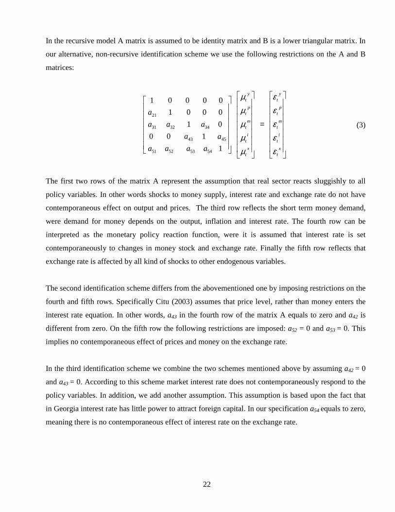
In the recursive model A matrix is assumed to be identity matrix and B is a lower triangular matrix. In

our alternative, non-recursive identification scheme we use the following restrictions on the A and B

matrices:

=

xt

it

mt

pt

yt

xt

it

mt

pt

yt

aaaa

aa

aaa

a

ε

ε

ε

ε

ε

µ

µ

µ

µ

µ

1

100

01

0001

00001

54535251

4543

343231

21

(3)

The first two rows of the matrix A represent the assumption that real sector reacts sluggishly to all

policy variables. In other words shocks to money supply, interest rate and exchange rate do not have

contemporaneous effect on output and prices. The third row reflects the short term money demand,

were demand for money depends on the output, inflation and interest rate. The fourth row can be

interpreted as the monetary policy reaction function, were it is assumed that interest rate is set

contemporaneously to changes in money stock and exchange rate. Finally the fifth row reflects that

exchange rate is affected by all kind of shocks to other endogenous variables.

The second identification scheme differs from the abovementioned one by imposing restrictions on the

fourth and fifth rows. Specifically Citu (2003) assumes that price level, rather than money enters the

interest rate equation. In other words, a43 in the fourth row of the matrix A equals to zero and a42 is

different from zero. On the fifth row the following restrictions are imposed: a52 = 0 and a53 = 0. This

implies no contemporaneous effect of prices and money on the exchange rate.

In the third identification scheme we combine the two schemes mentioned above by assuming a42 = 0

and a43 = 0. According to this scheme market interest rate does not contemporaneously respond to the

policy variables. In addition, we add another assumption. This assumption is based upon the fact that

in Georgia interest rate has little power to attract foreign capital. In our specification a54 equals to zero,

meaning there is no contemporaneous effect of interest rate on the exchange rate.

23

We summarize the results from the impulse response analysis in figure 54. In general these results go

in line with those found for our basic models. Both qualitative and quantitative characteristics remain

almost the same, showing high robustness of the impulse responses to different identification schemes.

Figure 5. Impulse Response Functions for SVAR Model

(Response to One S.D. Shock)

4 Note that impulse response functions from both alternative identification schemes are very similar. Because of this we only present the results of the third identification scheme.

-.005

0

.005

.010

0 5 10 15 20

a. Response of CPI to NEER

month

-.002

0

.002

.004

.006

0 5 10 15 20

b. Response of GDP to NEER

month

-.005

0

.005

.010

0 5 10 15 20


month -.002

0

.002

.004

.006

0 5 10 15 20


month

-.004

-.002

0

.002

0 5 10 15 20

e. Response of CPI to i

month -.004

-.002

0

.002

0 5 10 15 20

f. Response of GDP to i

month

24

A little difference is observed in the effect of exchange rate on prices. This effect becomes significant

after three months (against two in the baseline model) and dies out after nine months (against eight in

the baseline model). The effect of market interest rate on the price level is little bit lower and persists

shorter compared to our core model. No significant changes are observed in the shape of the rest

impulse response functions. On the whole the results confirm that obtained impulse responses are

robust under different assumptions.

VI. Monetary Aggregates

We further explore the role of different monetary aggregates. We first decompose M1 into currency in

circulation (CIC) and bank deposits (in national currency) to identifying which component of the base

money plays crucial role in monetary transmission. Then we use broad money measures (M2 and M35)

instead of base money (M1) used in our models so far.

Figure 6 demonstrates the impulse response results from the VAR model in which base money is

decomposed into currency in circulation and bank deposits.

Figure 6. Impulse Response Function for Monetary Aggregates (Response to One S.D. Shock)

5 The real GDP calculated by the second method is related to the foreign currency deposits, which are included in M3. As a result using this variable in the model with M3 will result in multicolinearity. However, as all the GDP measures give very similar results, we are not interested in solving this technical problem. Instead, we report the results from the model, which include M3 and real GDP measure, calculated by the first method.

-.002

0

.002

.004

.006

0 5 10 15 20

b. Response of GDP to CIC

month -.005

0

.005

.010

0 5 10 15 20

a. Response of CPI to CIC

month

25

As it can be seen from these results, it is CIC rather than bank deposits that determine both, inflation

and real GDP in Georgia. Moreover both, prices and output respond immediately and the positive

effect lasts for five and three months respectively. Finally neither inflation nor GDP responds

significantly to innovations to bank deposits (figures 6.c and 6.d).

The fact that prices and real economic activity (aggregate demand) responds insignificantly to Lari-

denominated bank deposits, may be the sign of the less developed banking system in Georgia. Figure 7

illustrates that the share of national currency deposits in M1 has increased in recent years, constituting

34% by the end of the period. The increasing share of deposits in base money leads to higher

sensitivity of the economy to total deposits and to the whole banking system. However, deposits to

CIC ratio still remains low in Georgia.

Figure 7. Share of Bank Deposits and Currency in M1

CIC

Bank Deposits

0%

20%

40%

60%

80%

100%

1/31

/199

6

1/31

/199

7

1/31

/199

8

1/31

/199

9

1/31

/200

0

1/31

/200

1

1/31

/200

2

1/31

/200

3

1/31

/200

4

1/31

/200

5

1/31

/200

6

1/31

/200

7

-.002

0

.002

.004

0 5 10 15 20

c. Response of CPI to Deposits

month -.001

0

.001

.002

.003

0 5 10 15 20

d. Response of GDP to Deposits

month

26

To examine the role of broad monetary aggregate we include M2 and M3 in the basic model instead of

M1. It appears that using broad money measures instead of base money does not change our results

from the baseline model significantly. These results are illustrated in figure 8. As in the model with

reserve money, the impact of money supply on prices and real output is positive and significant. But

this effect is persistent even for longer period (seven month).

Figure 8. Impulse Response Function for Monetary Aggregates (Response to One S.D. Shock)

These results for broad monetary aggregates are consistent to the existing economic literature. Number

of authors (Oomes and Ohnsorge, 2005, Dabla-Norris and Floerkemeier, 2006 among others) find

positive and significant price response to broad monetary aggregate, which includes foreign cash

holdings or foreign deposits. In general, our models, both with narrow and broad money measures

confirm that money supply is a significant tool in influencing inflation and aggregate demand.

However the role of bank deposits in monetary transmission process seems to be still limited.

-.005

0

.005

.010

0 5 10 15 20

a. Response of CPI to M2

month -.002

0

.002

.004

.006

0 5 10 15 20

b. Response of GDP to M2

month

-.002

0

.002

.004

.006

0 5 10 15 20


month -.002

0

.002

.004

0 5 10 15 20


month

27

VII. Summary and Conclusions

In the given paper we have analyzed the short-run effects of different transmission channels on the

price level and output in Georgia. The investigation covered several transmission channels which were

supposed to operate significantly in Georgia: the exchange rate channel, the interest rate channel, the

bank lending channel. In addition, the role of various monetary aggregates was explored.

In general, our results go in line with the existing empirical findings for other transition countries. The

positive and significant exchange rate pass-through to inflation, which is commonly observed in

transition economies, appears to be the characterizing feature of the Georgian economy. But sill,

compared to the previous results in the country the found effect is pretty low. This fact may point to

the evolutionary role of other transmission channels. For example the effect of the lending rate on

prices was found to be significant.

Table 4 summarizes other findings from VAR models. It appears that the second stage of the interest

rate pass-through, that is the effect of the bank lending rate on inflation, is significant. However,

because of the fact that NBG doesn’t use policy interest rate for conducting the monetary policy,

testing the first stage of the interest rate channel (the pass-through of the policy interest rate to lending

rate) is not feasible for Georgia.

Table 4. Summary of VAR Results

Variable Effect on Prices Effect on Output

Sign Significance Sign Significance

Exchange Rate + Yes + No Lending Rate - Yes - No Total Loans to Economy + No + No Loans in NC + Yes + No Loans in FC +/- No -/+ No M1 + Yes + Yes Currency in Circulation + Yes + Yes Demand Deposits (in GEL) + No + No M2 + Yes + Yes M3 + Yes + Yes

One of the findings deserving attention is the insignificant effect of demand deposits on GDP and

prices. Traditionally, Georgian economy was based on cash transactions. This was evidenced by the

28

high level of unobserved economy and dollarization, as well as low financial intermediation. However,

some indicators show that the situation is rapidly changing in Georgia. The increased role of banks in

transaction-making and in providing credit to the economy will improve overall economic activity and

enable the central bank to use its monetary policy tools more efficiently. Therefore, supporting private

banks should be the primary goal of NBG in the nearest future.

Finally, despite the multiple problems prevailing in the country, the growing significance of other

transmission channels (different from the exchange rate channel) over time enables us to believe that

the efforts undertaken by Georgian monetary authorities will give positive results in the future.

29

References

Bakradze G. and Billmeier A. 2007. Inflation Targeting in Georgia: Are We There Yet? IMF working papers. WP/07/193. Besimi F, Pugh G. and Adnett N. 2006. The monetary transmission mechanism in Macedonia: implications for monetary policy. Institute for Environment & Sustainability Research (IESR) working papers. Bernanke, B. S. and A. Blinder. 1988. Credit, Money and Aggregated Demand. American Economic Review Proceeding Papers. 78(2). 435.439. Billmeier A. and Bonato L., 2002. Exchange Rate Pass-Through and Monetary Policy in Croatia. IMF, Working Paper. WP/02/109. Cîtu F. 2003. A VAR Investigation of the Transmission Mechanism in New Zealand. Working papers of Reserve Bank of New Zealand Coricelli, Égert and MacDonald. 2006. Monetary transmission mechanism in Central and Eastern Europe: Gliding on a wind of change. BOFIT Discussion Papers 8/2006 Dabla-Norris E and Floerkemeier H. 2006. Transmission Mechanisms of Monetary Policy in Armenia: Evidence from VAR Analysis. IMF working papers. WP/06/248 Dabla-Norris E. Kim D. Zermeño M. Billmeier A. and Kramarenko V. Modalities of Moving to Inflation Targeting in Armenia and Georgia. IMF working papers. WP/07/133 Ganev G, Molnar K, Rybiński K, and Woźniak P. 2002. Transmission Mechanism of Monetary Policy in Central and Eastern Europe. Case Reports No. 52 Gigineishvili N. 2002. Pass-Through from Exchange Rate to Inflation: Monetary Transmission in Georgia. Journal Banki. N3(7). Golodniuk I. 2005. Evidence on the Bank Lending Channel in Ukraine. Paper presented at the Second Meeting of the UACES Study Group on Monetary Policy in Selected CIS Countries. Helsinki, February 10-11. Héricourt, J. 2005. Monetary Policy Transmission in the CEECs: Revisited Results Using Alternative Econometrics. University of Paris 1. Mimeo. Horvath C, Krekó J and Naszódi A. 2004. Interest Rate Pass-Through: The Case of Hungary. National Bank of Hungary Working Paper No.8. Horvath B and Maino R. 2006. Monetary Transmission Mechanisms in Belarus. IMF working papers. WP/06/246 Juks R. 2004. The Importance of the Bank Lending Channel in Estonia: Evidence from Microeconomic Data. Bank of Estonia Working Paper No. 6. Maliszewski W. 2003. Modeling Inflation in Georgia. IMF Working Paper. WP03/212

30

Matousek R and Sarantis N. 2006. The Bank Lending Channel and Monetary Transmission in Central and Eastern Europe. Paper presented at the 61st International Atlantic Economic Conference Berlin. March 15.19, 2006. Oomes, N. and Ohnsorge F. 2005. Money Demand and Inflation in Dollarized Economies: The Case of Russia. IMF Working Paper 05/144 Peersman G. and Smets F. 2001. The monetary transmission in Euro area: More evidence from VAR analysis. European central bank working papers. Pruteanu A. 2004. The Role of Banks in the Czech Monetary Policy Transmission Mechanism. Checz National Bank Working Paper No. 3. Sims C. 1986. Are forecasting models usable for policy analysis?, Federal Reserve Bank of Minneapolis Quarterly Review, 10, winter. Sims C and Zha T.1998. Does monetary policy generate recessions? Federal Reserve Bank of Atlanta, Working Paper 98-12. Starr A. 2004. Does Money Matter in the CIS? Effects of Monetary Policy on Output and Prices. US Department of Economics Working Paper Series. No. 2004-09

31

Appendix

Figure 1. Impulse Response Functions from Baseline Model

0

500000

1000000

1500000

2000000

2500000

3000000

35000001/

31/1

996

1/31

/199

7

1/31

/199

8

1/31

/199

9

1/31

/200

0

1/31

/200

1

1/31

/200

2

1/31

/200

3

1/31

/200

4

1/31

/200

5

1/31

/200

6

1/31

/200

7

M1 M2 M3

Monetary Ratios Dollarization Ratio – foreign currency denominated deposits placed with commercial banks to the total deposit liabilities.

Dollarization Ratio (M3) – foreign currency denominated deposits placed with commercial banks to the broad money (M3).

Velocity of Money Circulation reflects average number of single money unit usage in settlements within the given period of time. It is calculated by the following equation:

M

PYV = ,

Where V is velocity of money (M) in circulation, Y – real GDP, P – deflator of GDP, M – money supply (M2/M3).

Monetization Ratio – inverse value of velocity of money circulation.

Monetary Transmission Mechanism in Georgia - National Bank Of

Documents

Transcript of Monetary Transmission Mechanism in Georgia - National Bank Of