Monetary theory - Michel Beine · over, the CB may deviate from the rule to boost output. Monetary...

Monetary theoryECON 0231, University of Brussels, 2005

Michel BEINE

[email protected]

Universite Libre de Bruxelles, Belgique.

http://homepages.ulb.ac.be/∼mbeine

Monetary theory – p. 1/79

Chapter 3: Rules vs discretion and time inconsistency ofmonetary policy


Introduction, definitions and concept


Introduction

Macroeconomic equilibrium depends on present andfuture monetary policies → importance of expectations(see chapter 2).

In order to anticipate, agents can rely on monetary rules(ex: Taylor Rule).

General issue: is the adoption of a monetary rule (asopposed to discretionary MP) desirable ?

This raises the issue of incentives of agents to committo or to deviate from the rule.

example: if the CB commits to some inflation rule →expectations of workers and trade unions → bargainingon the level of the nominal wage → once the bargainingover, the CB may deviate from the rule to boost output.


Rules vs discretion

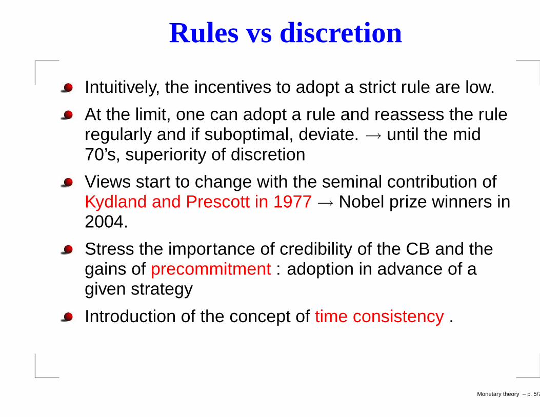
Intuitively, the incentives to adopt a strict rule are low.

At the limit, one can adopt a rule and reassess the ruleregularly and if suboptimal, deviate. → until the mid70’s, superiority of discretion

Views start to change with the seminal contribution ofKydland and Prescott in 1977 → Nobel prize winners in2004.

Stress the importance of credibility of the CB and thegains of precommitment : adoption in advance of agiven strategy

Introduction of the concept of time consistency .


Definition

Definition of time consistency : a particular policy istime-consistent if the planned response to newinformation remains the optimal response once the newinformation arrives .

A policy is time inconsistent if at time t + i it will not beoptimal to respond as originally planned.


Why is it important?

This leads to set up positive theories of the inflationrate: explains why some countries (i.e. South Americancountries, Turkey, Israel, ...) face over time high inflationrates.

Leads to normative theories: the optimal design of aCB, how to create incentives, how to control for possibledeviations. → one theory useful for the design of theEuropean Central Bank .


Section 1: Inflation in a discretionary regime


Inflation in discretion

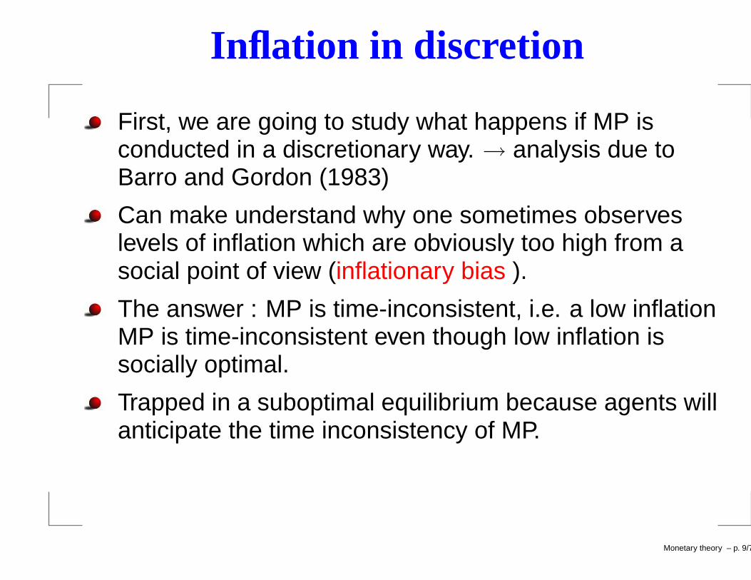
First, we are going to study what happens if MP isconducted in a discretionary way. → analysis due toBarro and Gordon (1983)

Can make understand why one sometimes observeslevels of inflation which are obviously too high from asocial point of view (inflationary bias ).

The answer : MP is time-inconsistent, i.e. a low inflationMP is time-inconsistent even though low inflation issocially optimal.

Trapped in a suboptimal equilibrium because agents willanticipate the time inconsistency of MP.


MP objectives

To define what is optimal → definition of the CBpreferences

At this stage government=central bank .

2 variables: output y and inflation π.

Loss function of Utility linear wrt output: authoritiesmaximize

U = λ(y − yn) −1

2π2

.

y: actual growth rate of output.


MP objectives

yn: natural growth rate of output. depends on the stocksof production factors, technical progress, etc ...

π: observed inflation rate

λ: weight of preference relative to output (as opposed toinflation). λ = ∞: government cares only foroutput;λ = 0: government only adverse to inflation;

authorities have an incentive to boost output becausethis increases the probability of being reelected andbecause there are distortions (tax, monopolies) leadingto yn inferior to the full-employment level.


Quadratic preferences

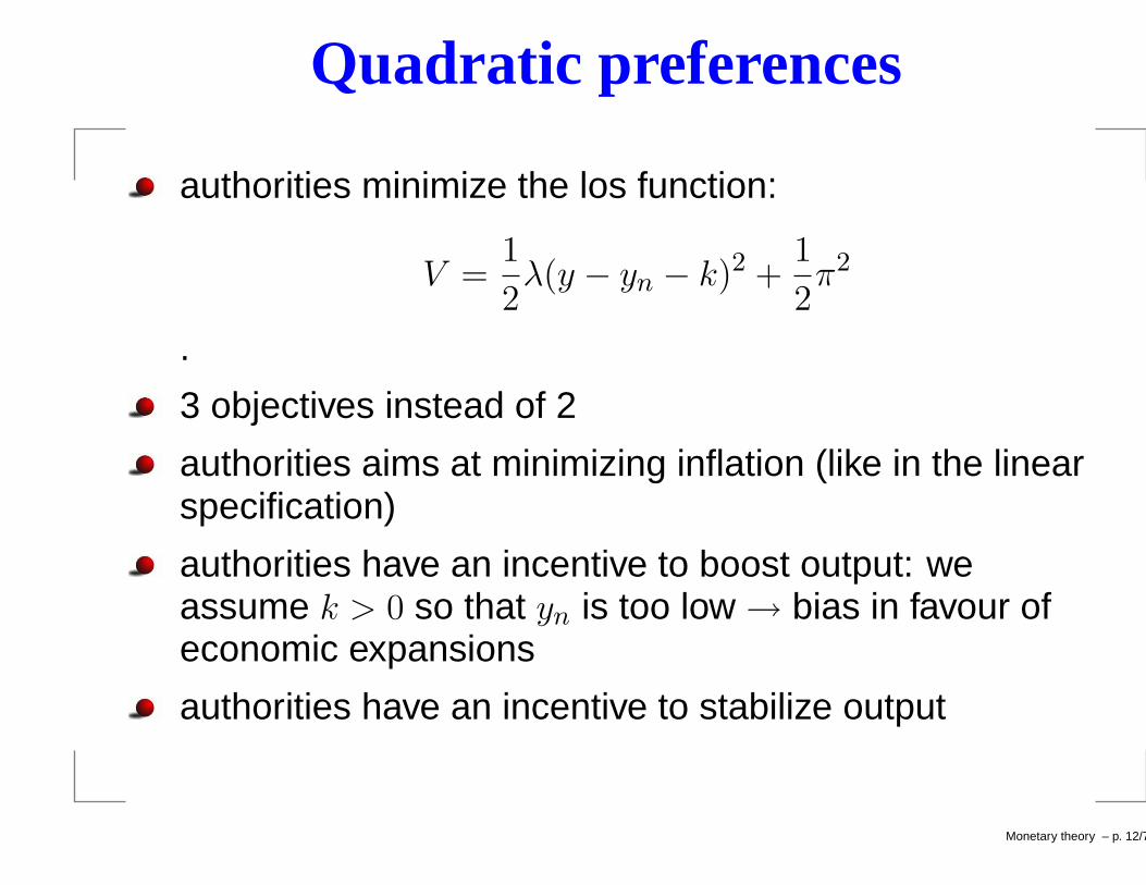
authorities minimize the los function:

V =1

2λ(y − yn − k)2 +

1

2π2

.

3 objectives instead of 2

authorities aims at minimizing inflation (like in the linearspecification)

authorities have an incentive to boost output: weassume k > 0 so that yn is too low → bias in favour ofeconomic expansions

authorities have an incentive to stabilize output


Comparing specifications

we can rewrite the quadratic specification as:

V = −λk(y − yn) +1

2π2 +

1

2λ(y − yn)2 +

1

2k2

.

−λk(y − yn): incentive to boost output12π2: incentive to minimize inflation12λ(y − yn)2 incentive to stabilize output around naturallevel.


Equilibrium in Barro-Gordon

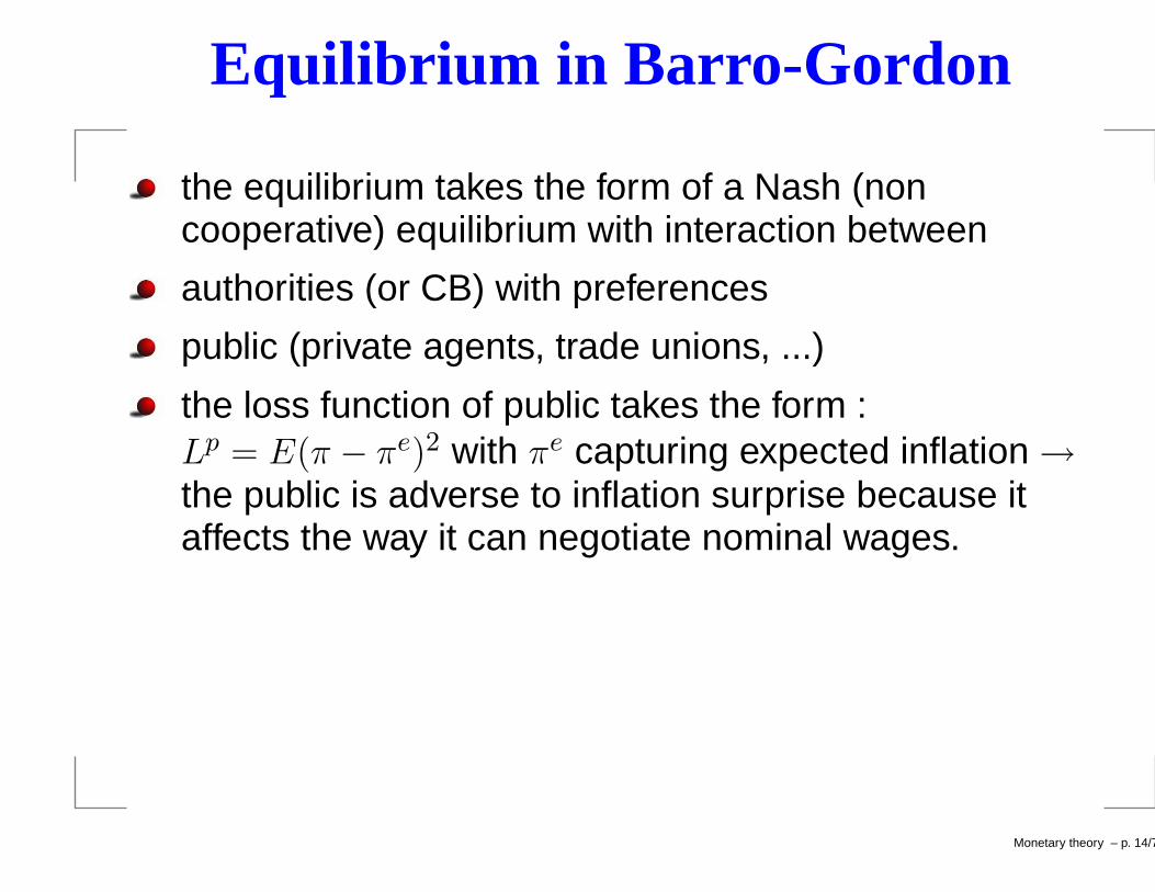
the equilibrium takes the form of a Nash (noncooperative) equilibrium with interaction between

authorities (or CB) with preferences

public (private agents, trade unions, ...)

the loss function of public takes the form :Lp = E(π − πe)2 with πe capturing expected inflation →the public is adverse to inflation surprise because itaffects the way it can negotiate nominal wages.


The economic structure

aggregate production is given by the Lucas surprisefunction (see AS in chapter 2) : y = yn + a(π − πe) + e

if π > πe, decrease of real wage and expansion ofoutput through the increase in labor demand

e is a AS shock

Relationship between inflation and MP isstraightforward: π = ∆m + ν

ν is money velocity shock

the instrument in this model is the money stock → noinvestigation of the optimal instrument (see chapter 4).

no uncertainty on the transmission of MP → choosingthe stance of MP is equivalent to choosing almostdirectly the level of inflation π.


Sequence of events

public sets up wages w on the basis of πe

realization of supply shock e

the CB (authorities) chooses ∆m

realization of ν which in turn determines π.

We see that authorities have an informationaladvantage over the public (private sector)→ possibilityto make surprises and to fool the public .


Inflation equilibrium

First consider the linear case (Barro-Gordon)

the CB maximizes

U = λ[a(π − πe) + e] −1

2π2

U = λ[a(∆m + ν − πe) + e] −1

2(∆m + ν)2

∂U∂∆m = 0 ⇒ ∆m = aλ > 0

π∗ = ∆m + ν = aλ > 0 .

The optimal inflation for the monetary authorities ispositive . This explains the inflationary bias .


Inflation equilibrium

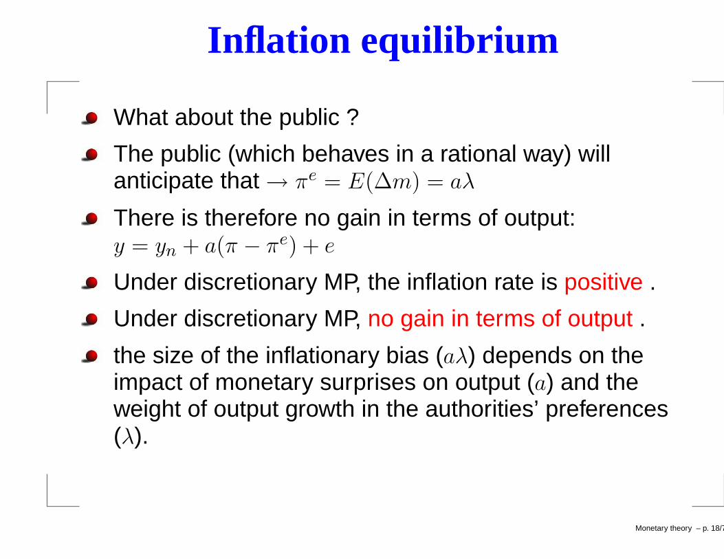
What about the public ?

The public (which behaves in a rational way) willanticipate that → πe = E(∆m) = aλ

There is therefore no gain in terms of output:y = yn + a(π − πe) + e

Under discretionary MP, the inflation rate is positive .

Under discretionary MP, no gain in terms of output .

the size of the inflationary bias (aλ) depends on theimpact of monetary surprises on output (a) and theweight of output growth in the authorities’ preferences(λ).


Explaining the inflationary bias

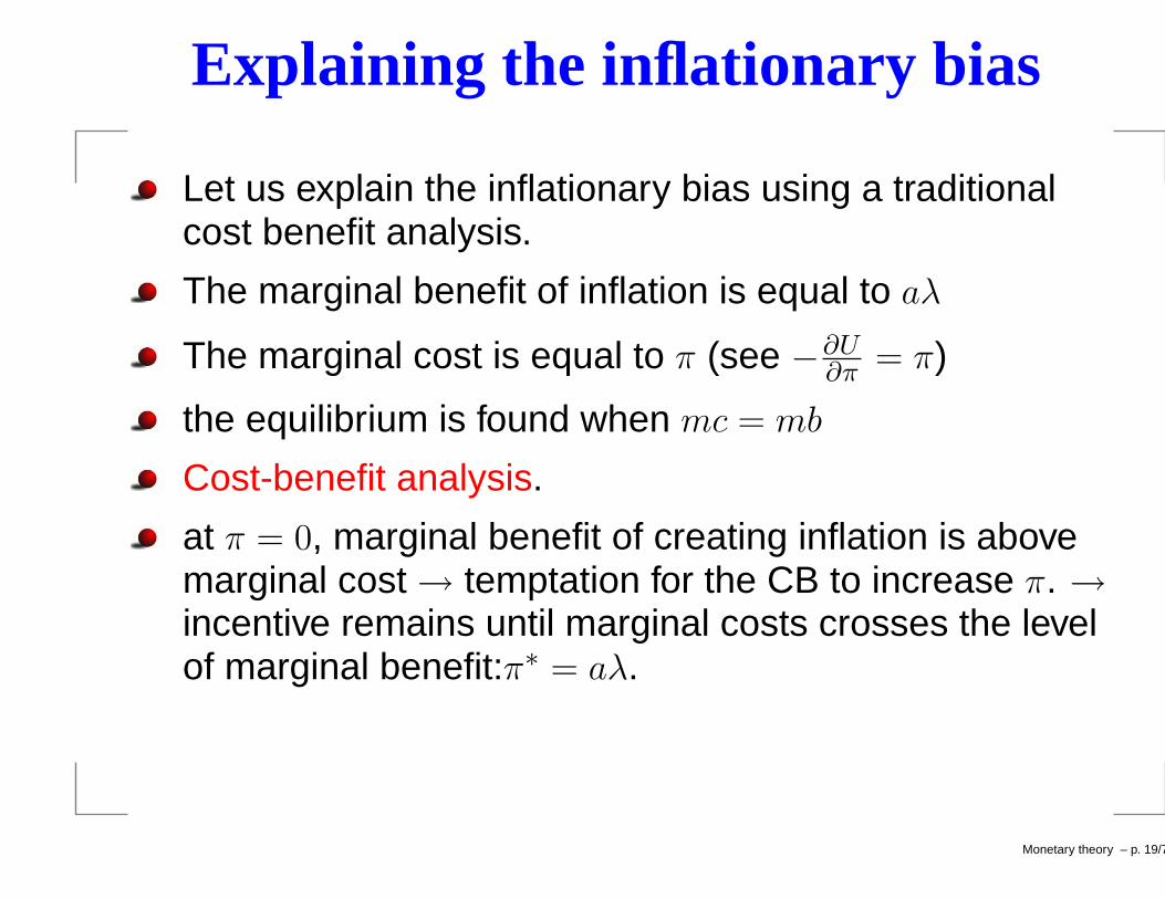
Let us explain the inflationary bias using a traditionalcost benefit analysis.

The marginal benefit of inflation is equal to aλ

The marginal cost is equal to π (see −∂U∂π = π)

the equilibrium is found when mc = mb

Cost-benefit analysis.

at π = 0, marginal benefit of creating inflation is abovemarginal cost → temptation for the CB to increase π. →incentive remains until marginal costs crosses the levelof marginal benefit:π∗ = aλ.


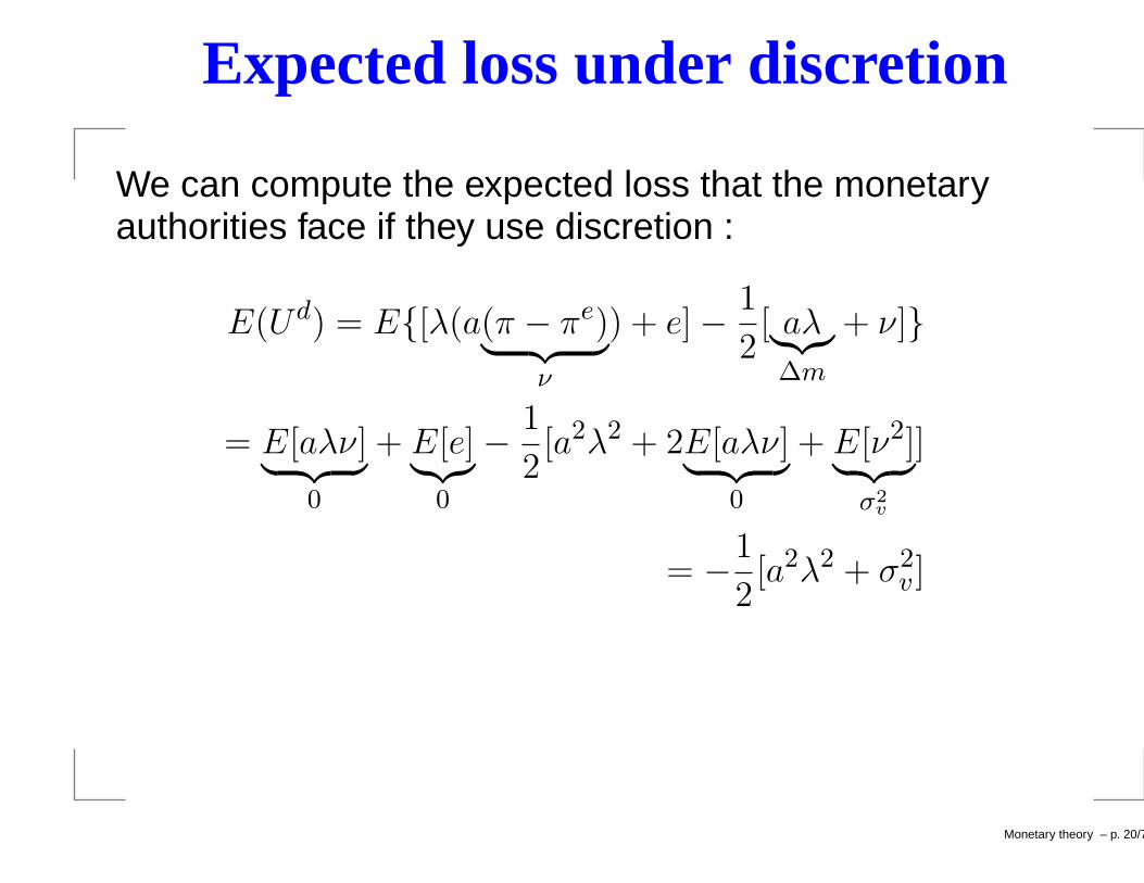
Expected loss under discretion

We can compute the expected loss that the monetaryauthorities face if they use discretion :

E(Ud) = E{[λ(a(π − πe)︸︷︷︸

ν

) + e] −1

2[ aλ︸︷︷︸

∆m

+ ν]}

= E[aλν]︸︷︷︸

0

+ E[e]︸︷︷︸

0

−1

2[a2λ2 + 2E[aλν]

︸︷︷︸

0

+ E[ν2]︸︷︷︸

σ2v

]

= −1

2[a2λ2 + σ2

v ]


Expected loss under discretion

The loss depends on the size of the inflationary biaswhich in turn depends on the weight in the loss functionand the impact of surprises : a2λ2.

The loss also depends on the size of the liquidityshocks: σ2

v

we can compare that with the expected loss if themonetary authorities can commit to follow a rule suchas :∆m = 0


Expected loss under commitment

We can compute the expected loss that the monetaryauthorities face if they commit and if they are credible :

E(U c) = E{λ(aν + e) −1

2v2}

= −1

2[σ2

v ] > E(Ud)

no inflationary bias any longer → supremacy of the rulewrt discretion if the monetary authorities can becredible .

But can they be credible ?


A Barro-Gordon example

UG = λ(y − yn) − 12fπ2

suppose that λ = 2 and f = 2

Up = −[π − πe]2

Consider 2 possible strategies of the government :π = 0 : virtuous monetary policy and π = 1 : inflationarymonetary policy

The public will anticipate the strategy of the government

we can compute the pay-offs related to each pair ofstrategy and looked for the equilibrium of the (noncooperative) game


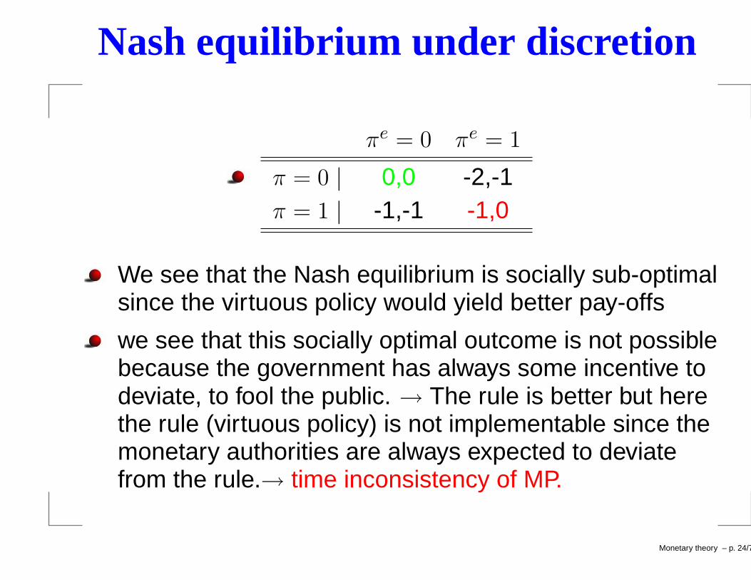
Nash equilibrium under discretion

πe = 0 πe = 1

π = 0 | 0,0 -2,-1π = 1 | -1,-1 -1,0

We see that the Nash equilibrium is socially sub-optimalsince the virtuous policy would yield better pay-offs

we see that this socially optimal outcome is not possiblebecause the government has always some incentive todeviate, to fool the public. → The rule is better but herethe rule (virtuous policy) is not implementable since themonetary authorities are always expected to deviatefrom the rule.→ time inconsistency of MP.


Inflationary bias in the quadratic case

V = 12λ[a(∆m + υ − πe) + e − k]2 + 1

2(∆m + υ)2

Since ν is observed only after the decision, monetaryauthorities take ν = 0

take the min: ∂V∂∆m = 0 ⇒ ∆m = a2λπe+aλ(k−e)

1+a2λ

We should compare that with the inflationary bias in thelinear case (∆m = aλ)

in this case,∆m depends on e: authorities want tostabilize output around the target → authorities respondto e



V = 12λ[a(∆m + υ − πe) + e − k]2 + 1

2(∆m + υ)2

we see that ∆m depends on πe → optimal monetarypolicy depends on expectations

we want to compute a value of ∆m which does notdepend on πe

Using rational expectations: πe = E(∆m) = aλk



we want to compute a value of ∆m which does notdepend on πe

Using rational expectations: πe = E(∆m) = aλk

πd = ∆m + ν

= aλk − (αλ

1 + aλ2)e + v

→ on average inflation is equal to aλk

no impact on output since πe = aλk

the inflationary bias is increasing in distortions k and(as before) in a and λ


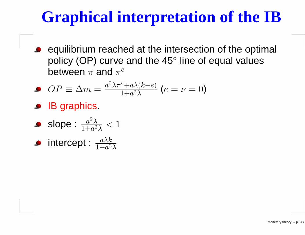
Graphical interpretation of the IB

equilibrium reached at the intersection of the optimalpolicy (OP) curve and the 45◦ line of equal valuesbetween π and πe

OP ≡ ∆m = a2λπe+aλ(k−e)1+a2λ

(e = ν = 0)

IB graphics.

slope : a2λ1+a2λ

< 1

intercept : aλk1+a2λ



the optimal inflation rate for πe = 0 is positive

as πe increases, authorities increase π in order to obtainthe same surprise and the same effect on output; butsince the cost of inflation increases,π increases lessquickly than πe

At the equilibrium : π = πe → intersection of the 2curves;



What about an increase of k: upward shift of OP → π∗

increases

increase of a: two opposite effects : increase of theslope of OP because impact of surprises stronger butintercept may decrease ; but the net effect is positive(π∗ = aλk)

Role of e : see the negative coefficient of e in the πd

equation: if there is a positive supply shock (positive onoutput) → restrictive monetary policy to stabilize output→ equilibrium inflation rate decreases.


Expected loss in the quadratic case

Substitute the value of πd in the loss function and takethe expectation in order to obtain the value of theexpected loss in the discretionary regime

V d =1

2λ[a(∆m + ν − πe) + e − k]2 +

1

2

[

πd]2

V d =1

2λ[(

1

1 + a2λ)e + aν − k]2 +

1

2

[

aλk − (aλ

1 + a2λ)e + ν

]2

Take the expectation and we can stress the role ofshocks; reminder : E(e) = E(ν) = 0;E(e2) = σ2

e ;E(ν2) = σ2ν


Expected loss in the quadratic case

One gets :E[V d] = 1

2 [( λ1+a2λ

)σ2e + (1 + a2λ)σ2

ν ] + 12λ(1 + a2λ)k2

We see the role of inflationary bias through λ(1 + a2λ)k2;

We see the role of shocks :σ2e and σ2

ν


Commitment in the quadratic case

Let us compare the discretionary outcome withcommitment; to do that, we have to assume a rulewhich, in the quadratic case, depends on e

Take a particular rule for ∆m in function of e(commitment)

rule: ∆mc = b0 + b1e ⇒ πe = E[∆mc] = b0

substitute πe in expected loss:V d = 1

2λ[a(b1e + υ) + e − k]2 + 12 [b0 + b1e + υ]2


Commitment in the quadratic case

Compute the expected value of V d et minimize thisexpected loss wrt to b0 and b1

we get (not explained): b0 = 0 ⇒ average inflation iszero

b1 = aλ1+a2λ

∆mc = aλ1+a2λ

e

using this value, we get the expected loss under(credible) commitment :E[V c] = 1

2 [( λ1+a2λ

)σ2e + (1 + a2λ)σ2

υ] + 12λk2


Cost of discretion in the quadratic case

E[V d] − E[Ud] = (aλk)2/2

(aλk)2/2 > 0 → discretion is costly

the cost is due to the higher average inflation rate(inflationary bias) : (aλk) while under commitment,inflation is zero.

Inflationary bias for two reasons: the CB has alwayssome incentive to fool the private sector once theinflation expectations have been set up; the CB cannotconvince that it will follow a strategy π = 0.


Summary of costs in both cases

Why is it impossible to convince the private sector ?

Assume that π = πe = 0. Can the CB convince that itwill target π = ∆m = 0 ?

In the linear case : marginal cost of inflation is :∂ 1

2π2

∂π = π =0; Marginal benefit: ∂λa[∆m+...]∂∆m = aλ

In the quadratic case : marginal cost identical : 0 .

Marginal benefit : −a2λ(π − πe) + aλk = aλk

the CB has always some incentive to deviate fromπ = 0.


The Friedman rule

The modern theory suggests that under a crediblecommitment, rule is better than discretion

Nevertheless, before, the debate favored the use ofdiscretion .

in the 50 and 60’s, Milton Friedman was a proponent ofa specific rule in term of monetary supply : ∆m = km :proposes a constant growth of monetary stock ; the aimis to get rid of counterproductive fine tuning policies (notto solve credibility problems).

opponents said that discretion was better than theFriedman rule because better response in terms ofstabilization and at the limit, one can follow the rulewhen optimal

see what happens in our analysis.Monetary theory – p. 37/79

The Friedman rule

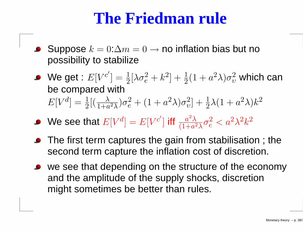
Suppose k = 0:∆m = 0 → no inflation bias but nopossibility to stabilize

We get : E[V c′ ] = 12 [λσ2

e + k2] + 12(1 + a2λ)σ2

υ which canbe compared withE[V d] = 1

2 [( λ1+a2λ

)σ2e + (1 + a2λ)σ2

υ] + 12λ(1 + a2λ)k2

We see that E[V d] = E[V c′ ] iff a2λ(1+a2λ

σ2e < a2λ2k2

The first term captures the gain from stabilisation ; thesecond term capture the inflation cost of discretion.

we see that depending on the structure of the economyand the amplitude of the supply shocks, discretionmight sometimes be better than rules.


Section 2: Solutions to the inflationary bias


The problem

The crucial issue : the authorities cannot commit to anon inflationary monetary policy

Why ? as soon as the public believes than π = ∆m = 0,the authorities will create inflation because the marginalbenefit>marginal cost.

How to solve the problem ? → 3 main proposedsolutions (rk : 2 other solutions but less important inpractice : see Walsh(2001, ch.8) for further information.


Solutions to time inconsistency

3 main solutions

Increase the actual marginal cost of an inflationarypolicy faced by the CB : introduction of reputation of theCB and extension to a dynamic game analysis

Increase the perceived marginal cost faced by theauthorities : Delegation of MP to a conservative andindependent central bank → most important in practice

Limit the flexibility of the authorities : adoption ofmonetary rules or adoption of inflation targeting regimewhich induce a cost when the CB deviates.


Section 2.1.: Reputation


Notion

In the preceding analysis, one big limitation : action attime t has no impact on the behaviour of agents at timet + 1 → inconsistent with rational agents

Here : take the time dependency into account through areputation effect of the monetary authorities

Notion: a vertuous behaviour of the CB will influencethe way the public sets its expectations of future policyand inflation.

As a result, we have a dynamic game between the CBand the public → extension of the previousBarro-Gordon static game with new results


Extending the dynamic game

Extension of the preferences of the authorities : Ut isreplaced by Vt =

∑∞

i=0 βiEt[Ut+i]

The authorities take into account the present and thefuture levels of utility.

The future levels are discounted : 0 ≤ β ≤ 1 is adiscount factor

2 extreme cases : β = 0 ⇒ static game : the authoritiesdo not take the future into account

β = 1 ⇒ the authorities put an equal weight to the futureoutcomes (unrealistic)


Extending the dynamic game

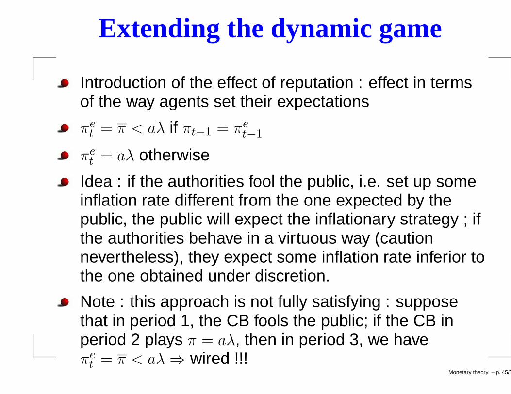
Introduction of the effect of reputation : effect in termsof the way agents set their expectations

πet = π < aλ if πt−1 = πe

t−1

πet = aλ otherwise

Idea : if the authorities fool the public, i.e. set up someinflation rate different from the one expected by thepublic, the public will expect the inflationary strategy ; ifthe authorities behave in a virtuous way (cautionnevertheless), they expect some inflation rate inferior tothe one obtained under discretion.

Note : this approach is not fully satisfying : supposethat in period 1, the CB fools the public; if the CB inperiod 2 plays π = aλ, then in period 3, we haveπe

t = π < aλ ⇒ wired !!!Monetary theory – p. 45/79

Is there an equilibrium?

Question: does an equilibrium exist for π = π < aλ ?

assume that πs = π ∀s < t ⇒ πet = π

What is the gain to deviate, to fool the public ? Let usassume e = ν = 0; assume that the CB wants to foolwith ∆m = ǫ > π

Net gain at time t : G = [aλ(ǫ − π) − 12ǫ2 − (−1

2π2)]

The first term captures the gain obtained throughfooling while the second term is the utility if the CB doesnot fool

Rearranging : G = aλ(ǫ − π) − 12(ǫ2 − π2)

Maximizing ∂G∂ǫ = 0 ⇒ ǫ = aλ

If the CB fools, it chooses the discretionary outcome.Monetary theory – p. 46/79

Equilibrium values for π

Let us find the possible equilibrium values for π bycomparing the temptation to cheat and the cost to cheat

Temptation (Gain) to cheat is given by:

G(π) = aλ(aλ − π) −1

2(aλ2 − π2)

G(π) =1

2(aλ − π2) ≥ 0

The temptation is positive for all π and reaches aminimum at the discretionary outcome.



Net cost to cheat that accounts for the intertemporalnature of the concept of reputation :

C(π) = β(−1

2π2) − β(−

1

2(aλ)2)

C(π) = β[(aλ)2 − π2]

The first term captures the cost if the CB does notcheat; the second term captures the cost if the CBcheats; since this cost is supported at time t + 1, it isdiscounted by the discount factor β.



Possible values for inflation are those for which the costto cheat is higher than the gain to cheat.

See Figure C(π)vs G(π) .

We see that πmin ≤ π ≤ aλ → reputation allows to reachan inflation rate inferior to the discretionary outcome.

One can show that : πmin = (1−β)(1+β)aλ < aλ → Importance

of the discount factor: the minimum inflation rate isdecreasing in β (interpret!!!) At the extreme, for β = 0,discretionary solution ; for β = 1,πmin = 0.


Additional remarks

Question of the coordination of inflation expectations:why all the private agents expect πe? One answer :labour unions tend to produce the same expectations

If the public’s sanction (in terms of higher inflationexpectations for next period) credible → the answer isnot straightforward but not addressed here.


Section 2.2.: Preferences


Idea

The idea is to have another type of preferences formonetary authorities

How ? By delegating to a central banker more averse toinflation than society (and the government): solutionproposed by Rogoff (1985)

Let us extend the previous preferences (quadraticversion): V = 1

2λ(y − yn − k)2 + 12(1 + δ)π2


Solution

δ: degree of conservatism of the central banker: moreaverse to inflation than society.

Why is it a solution ? We get :

πd = ∆m + ν

=aλk

1 + δ− (

αλ

1 + δ + aλ2)e + v


Optimal δ

We see that the inflationary bias has decreased;nevertheless no complete disappearance of the IB fornormal values of δ;

For δ → ∞, no IB; but is δ = ∞ optimal? the answer isno.

We see that the stabilization coefficient has decreased;there is some distortion in the response of monetaryauthorities → less answer and less stabilization

Auxiliary question: what is the optimal value of δ ?


Optimal δ

First compute the expected loss under conservatism

E[V d] = 12 [λk2 + λ( 1+δ

(1+δ+a2λ)2σ2

e + a2λσ2υ] + 1

2 [( aλk1+δ )2 +

( aλ1+δ+a2λ

)2σ2e + σ2

υ]

Maximizing wrt δ, i.e. ∂E[V d]∂δ = 0, we get :

δ = k2

σ2e

(1+δ+a2λ)3

1+δ ≡ g(δ)

Note that limδ→∞ g(δ) = k2

σ2e

> 0

graphically, the optimal δ is the one for which δ = g(δ);this means that we should look at the intersectionbetween the 45◦ line and the g(δ) function :graph optimal degree of conservatism.


Optimal δ

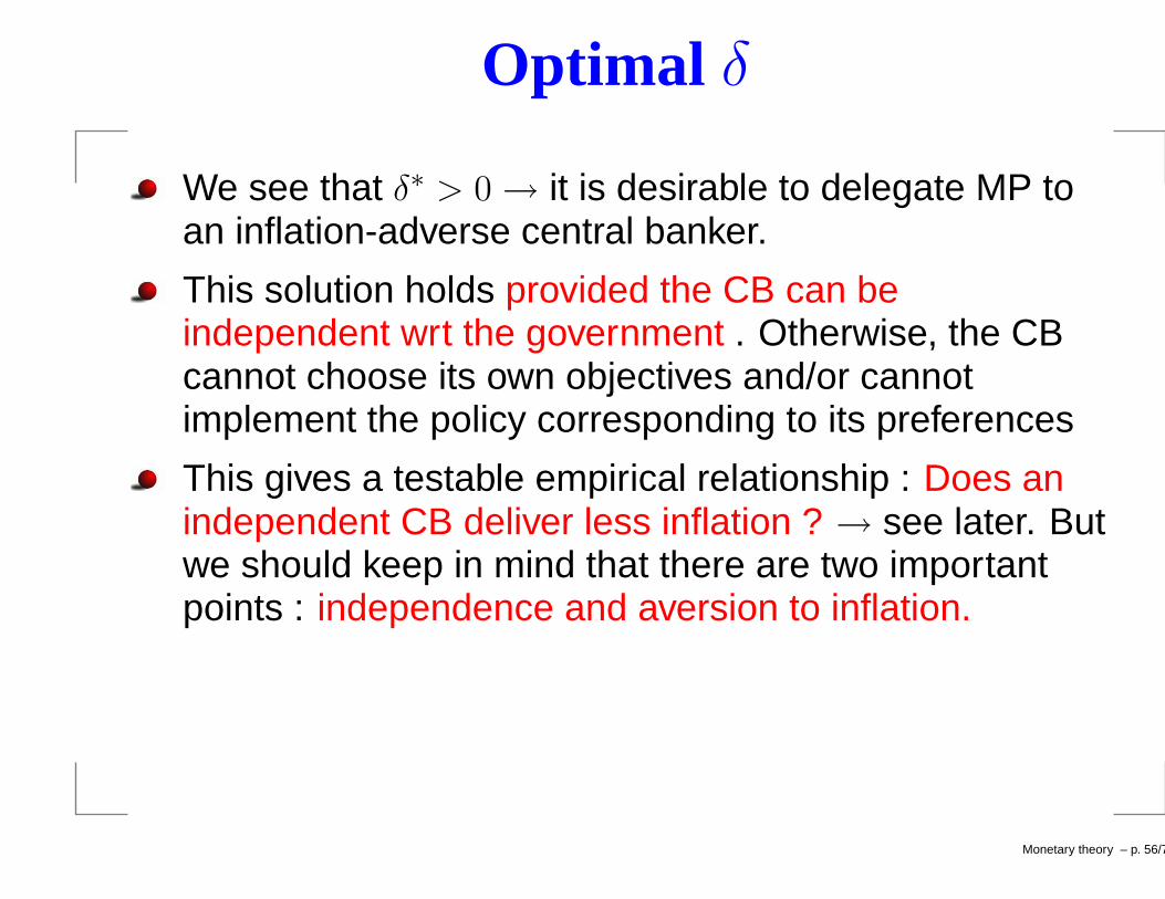
We see that δ∗ > 0 → it is desirable to delegate MP toan inflation-adverse central banker.

This solution holds provided the CB can beindependent wrt the government . Otherwise, the CBcannot choose its own objectives and/or cannotimplement the policy corresponding to its preferences

This gives a testable empirical relationship : Does anindependent CB deliver less inflation ? → see later. Butwe should keep in mind that there are two importantpoints : independence and aversion to inflation.


Optimal δ

This solution gives rise to some cost : trade-off betweenbias reduction and loss in terms of stabilization : if wecompute the variance of output : σ2

y = ( 1+δ1+δ+a2λ

)σ2e +a2σ2

ν

the variance of output is increasing wrt to δ : morevariability due to output shocks because distortion inthe stabilization response

This gives a second testable empirical proposition : Thevolatility of output is higher in countries in which the CBis relatively independent .


Section 2.3.: Inflation targeting


Idea of IT

Rather than working on preferences, one solution is toreduce the flexibility of MP

How ? By imposing a target to the central bank. Thistarget is on the level of inflation : Inflation Targeting .

First country to implement IT program wasNew-Zealand in 1989 with an explicit target of 2prcents; the governor of the CB has to account for theperformances and might face some sanctions likegetting fired , ...

Other examples : Canada, UK, Israel; What about theECB : this is a mixed regime (the two-pillars strategy)and in no case is the 2 percent an explicit target.


Idea of IT

IT is only one way of reducing the freedom of the CB →other ways like

Exchange rate systems : fully fixed like in a monetaryunion or currency boards (Argentina) , adjustable likethe EMS. One argument in favor of EMS for countrieslike Italy or Belgium

Two different types of IT :

Flexible rules : penalty if deviation from the inflationtarget πT but deviation is allowed → possibility offollowing other goals than inflation

Strict rules : the CB has to adopt a given rule . Example: Friedman rule → Effects similar to a credible rule seenbefore

→ Let us investigate the effects of flexible rules.Monetary theory – p. 60/79

IT with flexible rules

The CB is penalized if the performance deviates fromthe target : more general loss function;

Example: Bank of Canada: in 2005, target band interms of inflation rate : between 1 and 3 % with amedian of 2%

Nevertheless, room to deviate from the target but in thiscase penalized



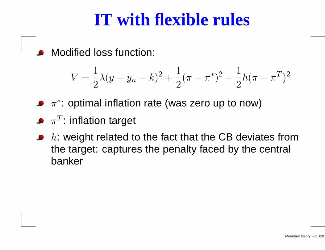
Modified loss function:

V =1

2λ(y − yn − k)2 +

1

2(π − π∗)2 +

1

2h(π − πT )2

π∗: optimal inflation rate (was zero up to now)

πT : inflation target

h: weight related to the fact that the CB deviates fromthe target: captures the penalty faced by the centralbanker

Note that because π∗ 6= 0 now, inflation rate underdiscretion becomes:

πd = ∆m + ν

= π∗ + aλk − (αλ

1 + aλ2)e + v




V =1

2λ(y − yn − k)2 +

1

2(π − π∗)2 +

1

2h(π − πT )2





Inflation under IT


V =1

2λ(y − yn − k)2 +

1

2(π − π∗)2 +

1

2h(π − πT )2





Inflation under IT

VCB = 12λ[a(∆m + υ − πe) + e − k]2 + 1

2(∆m + υ − π∗)2 +12h(∆m + υ − πT )2

∂V∂∆mT = 0 (υ = 0 because unknown)

∆mT = 11+h+a2λ

(a2λπe − aλe + aλk + π∗ + hπT )

Using rational expectation hypothesis:∆mT = 1

1+h+a2λ(a2λπe − aλe + aλk + π∗ + hπT )

∆mT = aλk+π∗+hπT

1+h − ( aλ1+h+a2λ

)e

∆mT = π∗ + aλk1+h + h(π∗

−πT )1+h − ( aλ

1+h+a2λ)e


Inflation under IT

If we assume that the CB targets the optimal inflationrate, i.e. π∗ = πT

∆mT = π∗ + aλk1+h − ( aλ

1+h+a2λ)e

We see that we get a lower inflationary bias : aλk1+h < aλk

This at the expense of a lower stabilization coefficient

We see that inflation targeting reduces the marginalcost of inflation and reduces the inflationary bias butleads to a distortion of the answer of monetary policy interms of stabilization.


Comparison with conservative CB

The h parameter (penalty if deviation) plays exactly thesame role of the δ parameter in the context of MPdelegation (see before)

We can thus applied the same conclusions as before

There is a an optimal positive h

h = ∞ is suboptimal

Inflation targeting should lower the inflationary bias butincrease output volatility wrt to discretion.


Section 4. Policy implications: the independence of the CB


independence and delegation

Solution to time inconsistency issue : delegation to aninflation CB

This solution works if the CB is independent from thegovernment

Since preferences are not directly observable, the onlyway is to test the relationship between independenceand the level of inflation

it is therefore assume that inflation aversion goes handin hand with the degree of independence

Based on the theory, the relationship should benegative.


How to measure independence

There are two types of independence

Political independence : ability of the CB to choose thefinal objective of monetary policy → freedom to choosea low inflation rate

Economic independence : ability to choose theinstruments of monetary policy in order to reach thechosen goals.

Analysis proposed by Grilli, Masciando and Tabellini(1991, Economic policy) on the 18 major central banks


political independence

degree or political independence depends on

the way governors and policy board members areappointed

relations with the government

constitution or status of the CB

indexes of political independence.

Most (politically) independent CBs: Bundesbank,Nederlandsche Bank, Fed


Economic independence

degree or economic independence depends on

the extent to which fiscal deficits can be financed bymoney

control of the CB over policy instruments

Results: indexes of economic independence.

Most (economically) independent CBs: Bundesbank,Bank of Swiss, Bank of Canada, National Bank ofBelgium


Degrees of independence

Does economic and political independence go hand inhand ?

Not always : see relationship between both types.

a significant number of CBs in the South-East quadrant.


Impact of independence

Econometric analysis : cross section analysis (no timeseries dimension)

estimated relationship :infi = int + β1ecindi + β2poindi + β3EMSi + ǫi

EMS equal 1 if country i belongs to the Europeanexchange rate mechanism, 0 otherwise

estimated over the 1950-1989 period and subperiods of10 years

Results : Not always : see Impact of independence.

Conclusion: economic independence matters, politicalindependence less !! . → support for the theory.


Is there a cost?

Theory says that delegation to inflation-adverse CBlowers the response in terms of stabilisation

→ see relationship between output variability andindependence

2 measures : output growth and output variability

same type of econometric models

see Cost of independence.

No significant relationship between independence andoutput variability → no support for the theory


Conclusion

Economically CBs are found to generate less inflation

More conservative CBs do not seem to generate adistorted response in terms of stabilisation → no realcost to conservatism

→ Strong empirical support for independence andconservatism.


Updating: independence of the ECB

The ECB is one of the most independent banks in theworld

See comparison of the major central banks usingvarious measures

Updating indexes of independence.

The ECB is the most independent for all indexes

the ECB is even more independent than the formerBundesbank → implicit recognition of the importance ofthe issue of time inconsistency and the need to avoid itsconsequences.


Accontability

Recently, attention shifts to accountability of centralbanks

idea: in a democracy, the CBs should account to thepopulation, the parliament or the government

The concept of accountability encompasses 3dimensions:

Clarification of ultimate objectives of MP

Transparency of monetary policy

Ultimate control of the government of parliament overthe MP. (might be a problem for independence).


Measuring accountability

Measures of 3 dimensions to compute an index ofaccountability

analysis conducted on 5 major central banks includingthe ECB

results :see Accountability Measures.

low accountability of the ECB due to poor transparencyand poor final responsibility


Monetary theory - Michel Beine · over, the CB may deviate from the rule to boost output. Monetary...

Documents

Transcript of Monetary theory - Michel Beine · over, the CB may deviate from the rule to boost output. Monetary...