Monetary Policy in the Small Open Economy

with Market Segmentation *

Jae Hun Shim†

Department of Economics, University of Bath

September 2016 (This Version, July 2017)

Abstract

We extend a New Keynesian small open economy DSGE model with non-tradable goods and inter-mediate inputs. Firstly, we show that the optimal monetary policy faces a trade-off between compositedomestic inflation and output gap stabilization due to net exports externalities. Secondly, we rank alter-native monetary policy rules associated with welfare and show that setting graduate interest rates towardstheir target levels rather than an immediate response is desirable. However, when the economy is highlyexposed to foreign goods market and non-tradable productivity shocks, the CPI-based Taylor rule canbe the best alternative policy. Lastly, we identify linkages between final and intermediate sectors andexplain “sectoral heterogeneity” under the optimal policy and alternative monetary policy regimes.

Keywords: Small open economy, Net exports externalities, Optimal monetary policy, Non-tradable

goods, Intermediate inputs

JEL Classification Numbers: E52, F3, F41

1 Introduction

There has been a great debate whether central banks in an open economy should take into account

fluctuations in the exchange rate for the monetary policy design or follow a purely inward looking mone-

tary policy by targeting domestic inflation. The open economy macroeconomic literature has explored the

optimal monetary policy in the absence of non-tradable sectors and argues that the monetary policy in a

*I am greatly indebted to Christopher Martin for his valuable comments. Also, I would like to thank Charles Engel, Jordi Gali,Alexander Mihailov, Bruce Morley and Harald Uhlig for useful comments and help.

†Address: Department of Economics, University of Bath, Bath, BA2 7AY, UK, e-mail: jhs30@bath.ac.uk.

1

small open economy is isomorphic to the closed economy (see, for example, Clarida et al. (2001), Gali &

Monacelli (2005), Faia & Monacelli (2007) and De Paoli (2009)).

This paper analyses the optimal monetary policy in a small open economy characterised by relative

prices (the terms of trade and the relative home producer price), and compare different monetary policy rules

in a welfare analysis. In our model, the relative prices through the expenditure switching effect between non-

tradable goods and home (foreign) tradable goods are key factors for explaining the dynamics of the small

open economy and the optimal monetary policy, and capturing a role for non-tradable sectors. Empirically,

roughly 40% of GDP comes from consumption of non-tradable goods as shown by Dotsey & Duarte (2008)

and Stockman & Tesar (1995)1, and non-tradable goods play critical roles in explaning the real exchange rate

(see, for example, Burstein et al. (2005), Obstfeld & Rogoff (2007), Dotsey & Duarte (2008) and Rabanal

& Tuesta (2013)). This implies that the presence of non-tradable sectors alters the dynamics of the economy

by stochastic shocks and the optimal policy through risk sharing and market clearing conditions.

Extensive studies have analysed the optimal monetary policy and terms of trade effects in the absence of

non-tradable sectors. Corsetti & Pesenti (2001) find that in contrast to the closed economy, positive domestic

monetary shocks can reduce domestic welfare due to terms of trade effects. In the open economy, a positive

monetary shock induces depreciation of the nominal exchange rate and the terms of trade and CPI inflation

worsens purchasing power for a given short term sticky wage or home production price. The negative terms

of trade effects working through nominal exchange rate dynamics can be larger than the positive effects of

aggregate demand. Clarida et al. (2001) and Gali & Monacelli (2005) develop a small open economy New

Keynesian model with Calvo (1983) type staggered price setting and monopolistic competition and argue

that strict domestic tradable inflation targeting is the optimal policy. Also, they compare alternative monetary

policy regimes using a welfare analysis and argue that while the domestic tradable inflation-based Taylor

rule generates the lowest welfare losses, the exchange peg (PEG) policy leads to the highest welfare losses

in response to the composite of productivity and foreign output shocks. Faia & Monacelli (2007) analyze

the optimal monetary policy using a Rotemberg (1982) type sticky price model which is characterized by

home bias in consumption and show that since the optimal monetary policy requires quantatively negligible

volatile domestic tradable inflation in response to the productivity shocks, strict domestic tradable inflation

targeting is a good approximation to the optimal policy. Also, De Paoli (2009) shows that the domestic

1The literature computes the average share of personal consumption of services in GDP for the share of non-tradable consump-tion. Stockman & Tesar (1995) use data from the seven largest industrial countries (Canada, France, Germany, Italy, Japan, UK andUS) during 1970-1984 and Dotsey & Duarte (2008) use the US data during 1973-2004.

2

tradable inflation-based policy rule is superior to consumer price inflation-based policy rule and PEG except

for implausibly high values of the elasticity of substitution between home and foreign goods in response to

the composite shocks (productivity, markup, fiscal and external shocks)

So far, there have been many developments embedding non-tradable sectors in the open economy

macroeconomic models such as Obstfeld & Rogoff (2000), Obstfeld & Rogoff (2007), Dotsey & Duarte

(2008) and Rabanal & Tuesta (2013). The literature mostly focuses on the role of non-tradable sectors in ex-

plaining real exchange rate movement rather than investigating the optimal monetary policy or externalities

from the movement in the relative prices. While Lipinska (2015) investigates the optimal monetary policy

with non-tradable goods using the welfare loss function and gives penalties on the fluctuations away from

the target levels, the optimal policy is characterised by fixed loss function coefficients from calibrated pa-

rameter values. Also, Devereux et al. (2006) examine the optimal monetary policy with non-tradable goods

but they do not embed tradable sectors. Thus, their model does not capture a trade-off between composite

domestic inflation and the output gap in the optimal policy.

Our analysis has three main contributions. Firstly, by embedding non-tradable goods, we identify an ad-

ditional expenditure switching effect between home non-tradable goods and home (foreign) tradable goods.

Households optimally choose the combination between home tradable and non-tradable goods, and imports

depending on the relative prices. Thus, in addition to the choice between home and foreign tradable goods,

they also choose between non-tradable goods and home (foreign) tradable goods. This implies that we ob-

serve net exports externalities arising from imperfect substitutability between tradable goods, non-tradable

goods and imports. We identify net exports externalities in the optimal allocation and the optimal monetary

policy. The optimal allocation requires eliminating net exports externalities along with the monopolistic

distortions. Thus, strict domestic tradable inflation targeting in the open economy is no longer optimal in

the presence of non-tradable sectors. Rather, the optimal policy requires to stabilize both tradable and non-

tradable inflation by eliminating the externalities. However, since stabilizing tradable inflation, non-tradable

inflation and the output gap is not attainable without fiscal instruments, the central bank faces a trade-off

between stabilizing composite domestic inflation and the output gap due to the externalities.

Secondly, we compare alternative monetary policy rules in a welfare analysis and show that ranking of

monetary rules crucially depends on types of shocks and parameter values. In response to tradable pro-

ductivity shocks, the agumented composite domestic inflation-based Taylor rule (ADT) leads to the lowest

welfare losses. The partial adjustment of the interest rates of ADT reduces a volatility of composite do-

3

mestic inflation and welfare losses. For non-tradable productivity shocks, the CPI-based Taylor rule (CTR)

outperforms other alternative policy rules. While CTR and ADT symmetrically stabilize composite domes-

tic inflation, CTR further reduces a volatility of the relative price gap and thereby stabilizing the output gap.

Importantly, we find that under the conventional inflation coefficient, the composite domestic inflation-based

Taylor rule (DTR) generates the highest welfare losses by tradable productivity, non-tradable productivity

and composite shocks. Thus, setting graduate interest rates towards their target levels rather than an imme-

diate response appears to be desirable unless the central bank responds sufficiently aggressive to composite

domestic inflation. However, when the economy is highly exposed to foreign goods markets (i.e., high

degree of openness, weights on tradable goods and elasticities of substitution between home and foreign

tradable goods) and non-tradable productivity shocks, CTR can be the best alternative policy.

Lastly, in contrast to the standard open economy DSGE model, we also introduce intermediate sectors in

order to analyse the impact of stochastic shocks on the intermediate sectors which consist of approximately

50% of gross output across countries as shown by Jones (2011). In our model, markets are segmented so

that we have three sectors; a final non-tradable sector, a final tradable sector and an intermediate sector.

Dotsey & Duarte (2008) introduce intermediate sectors along with the presence of non-tradable sectors us-

ing an otherwise standard open-economy macro model and highlight the critical role of nontradable goods

in explaining the real exchange rate. They assume that in the non-tradable sectors, output of monopolisti-

cally competitive firms is used as both final non-tradable goods and non-tradable intermediate inputs, and

final tradable sectors combine intermediate inputs (home and foreign tradable intermediate inputs and non-

tradable intermediate inputs) so that they do not explicitly distinguish final and intermediate sectors, thereby

excluding an analysis of intermediate sectors. Thus, the main departure in this paper is that in order to shed

light on the intermediate sectors, we distinguish final and intermediate sectors by embedding separate final

and intermediate non-tradable sectors and assuming the standard production function of final tradable sec-

tors. We compare dynamics of main variables in intermediate sectors under alternative monetary regimes

and find that under the optimal policy, intermediate sectors are symmetrically beneficial from the stochastic

shocks (tradable and non-tradable sector productivity shocks). However, under CTR, ADT and PEG, while

the stochastic shocks have symmetric impact on the final and intermediate tradable sectors, it does not have

symmetric impact on the final and intermediate non-tradable sectors due mainly to the sectoral capacity to

engage in international trade and the substitutability between home and foreign tradable goods (intermediate

inputs).

4

The paper is organized as follows: Section 2 briefly describes sectoral output and productivity fluctua-

tions in response to sectoral productivity shocks. Section 3 describes the small open economy model with

non-tradable goods and intermediate sectors, and derives the optimal monetary policy. Section 4 presents

calibrated values and quantitative results. Section 5 concludes.

2 Stylised Facts of Market Segmentation

2000 2002 2004 2006 2008 2010 2012 2014 2016-0.1

-0.06

-0.02

0

0.02

0.06

0.1

TS NT TIS NTIS TS Productivity NTS Productivity

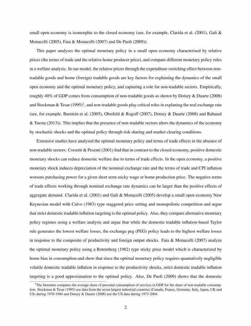
Figure 1: Sectoral Output and Productivity in Korea

NOTE: TS, NTS, TIS and NTIS refer to tradable sectors, non-tradable sectors, tradable intermediate sectorsand non-tradable intermediate sectors, respectively. Variables are presented in percentage deviations froman Hodrick-Prescott (HP) filtered trend and estimated from 2000q1 to 2016q4. Following Burstein et al.(2005), Corsetti et al. (2008) and Dotsey & Duarte (2008), we regard non-tradable intermediate output aswholesale and retail services and transportation (distribution services). Source: The Bank of Korea andFederal Reserve Economic Data.

In order to explore the sectoral heterogeneity in a small open economy in response to sectoral produc-

tivity shocks, Figure 1 shows sectoral output and productivity fluctuations in South Korea2 during 2000q1-

2016q4. The green (grey) line corresponds to tradable (non-tradable) productivity shocks3. Three main styl-

ized facts stand out. Firstly, we observe the heterogeneity of sectoral output fluctuations between tradable

and non-tradable sectors (final and intermediate sectors) in response to sectoral productivity shocks. Sec-

2Korea has one of the most open goods markets in the world and a small open economy which is unable to influence the foreigninterest rate, output and prices, and the central bank in Korea is following the CPI-based Taylor rule. During the period given,the share of consumption of non-tradable goods and that of intermediate goods consist of approximately 40% and 50% of GDP,respectively.

3As Figure 1 shows, tradable and non-tradable productivity shocks are highly correlated, corr(σH,T ,σH,N) = 0.53 and thus, thevertical green (grey) line corresponds to the quarter when tradable (non-tradable) sector productivity changes due to changes insectoral labour market conditions and distinctively dominates the other.

5

ondly, while non-tradable sector productivity shocks led to broadly symmetric fluctuations of sectoral output,

positive tradable productivity shocks had a negative effect on non-tradable intermediate sector. Lastly, we

observe relatively large fluctuations of tradable intermediate sector output in response to tradable productiv-

ity shocks4.

3 A Small Open Economy Model

The model is a two-country New Keynesian DSGE model with non-tradable goods and intermediate

sectors. The baseline framework for the open economy follows Gali & Monacelli (2005), Sutherland (2005),

Obstfeld & Rogoff (2007) and Meier (2013). We extend the benchmark for small open economy New

Keynesian DSGE model with non-tradeable goods and intermediate inputs.

3.1 Households

The world is composed of a small home economy and the large foreign country. The home country is

small since it is unable to influence the foreign interest rate, output and prices. Households on the subinterval

[0, n) live in the home country (denoted by h) and households on the subinterval (n, 1] live in the foreign

country (denoted by f).

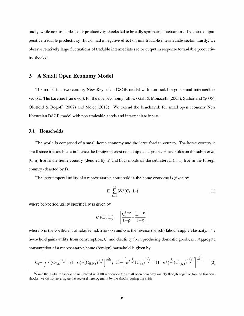
The intertemporal utility of a representative household in the home economy is given by

E0

∞

∑t=0

βtU(Ct, Lt) (1)

where per-period utility specifically is given by

U (Ct, Lt) =

[C1−ρ

t

1−ρ−Lt

1+ϕ

1+ϕ

]

where ρ is the coefficient of relative risk aversion and ϕ is the inverse (Frisch) labour supply elasticity. The

household gains utility from consumption, Ct and disutility from producing domestic goods, Lt . Aggregate

consumption of a representative home (foreign) household is given by

Ct=[σ

1ω (CT,t)

ω−1ω +(1−σ)

1ω (CH,N,t)

ω−1ω

] ω

ω−1; Cf

t=

[σ

f1

ω f (CfT,t)

ω f−1ω f +(1−σ

f )1

ω f (CfF,N,t)

ω f−1ω f

] ω f

ω f−1(2)

4Since the global financial crisis, started in 2008 influenced the small open economy mainly though negative foreign financialshocks, we do not investigate the sectoral heterogeneity by the shocks during the crisis.

6

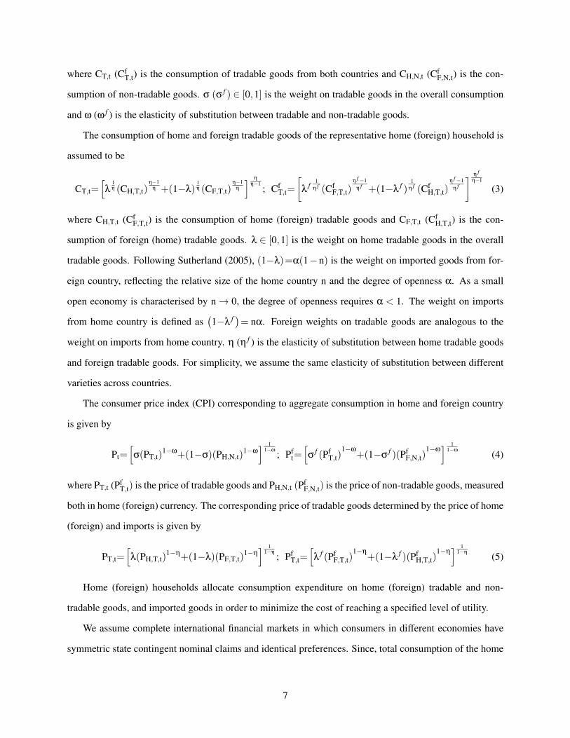
where CT,t (CfT,t) is the consumption of tradable goods from both countries and CH,N,t (Cf

F,N,t) is the con-

sumption of non-tradable goods. σ (σ f ) ∈ [0,1] is the weight on tradable goods in the overall consumption

and ω (ω f ) is the elasticity of substitution between tradable and non-tradable goods.

The consumption of home and foreign tradable goods of the representative home (foreign) household is

assumed to be

CT,t=[λ

1η (CH,T,t)

η−1η +(1−λ)

1η (CF,T,t)

η−1η

] η

η−1; Cf

T,t=

[λ

f1

η f (CfF,T,t)

η f−1η f +(1−λ

f )1

η f (CfH,T,t)

η f−1η f

] η fη−1

(3)

where CH,T,t (CfF,T,t) is the consumption of home (foreign) tradable goods and CF,T,t (Cf

H,T,t) is the con-

sumption of foreign (home) tradable goods. λ ∈ [0,1] is the weight on home tradable goods in the overall

tradable goods. Following Sutherland (2005), (1−λ)=α(1−n) is the weight on imported goods from for-

eign country, reflecting the relative size of the home country n and the degree of openness α. As a small

open economy is characterised by n→ 0, the degree of openness requires α < 1. The weight on imports

from home country is defined as(1−λ f

)= nα. Foreign weights on tradable goods are analogous to the

weight on imports from home country. η (η f ) is the elasticity of substitution between home tradable goods

and foreign tradable goods. For simplicity, we assume the same elasticity of substitution between different

varieties across countries.

The consumer price index (CPI) corresponding to aggregate consumption in home and foreign country

is given by

Pt=[σ(PT,t)

1−ω+(1−σ)(PH,N,t)1−ω] 1

1−ω

; Pft=[σ

f (PfT,t)

1−ω+(1−σ

f )(PfF,N,t)

1−ω] 1

1−ω

(4)

where PT,t (PfT,t) is the price of tradable goods and PH,N,t (Pf

F,N,t) is the price of non-tradable goods, measured

both in home (foreign) currency. The corresponding price of tradable goods determined by the price of home

(foreign) and imports is given by

PT,t=[λ(PH,T,t)

1−η+(1−λ)(PF,T,t)1−η] 1

1−η

; PfT,t=

[λ

f (PfF,T,t)

1−η+(1−λ

f )(PfH,T,t)

1−η] 1

1−η

(5)

Home (foreign) households allocate consumption expenditure on home (foreign) tradable and non-

tradable goods, and imported goods in order to minimize the cost of reaching a specified level of utility.

We assume complete international financial markets in which consumers in different economies have

symmetric state contingent nominal claims and identical preferences. Since, total consumption of the home

7

household is given by PtCt= PH,T,tCH,T,t+PF,T,tCF,T,t+PH,N,tCH,N,t , the per-period budget constraint for the

household is given by

PtCt + ∑qt+1∈q

Qa (qt+1|qt)B(qt+1|qt) ≤ Bt +WtLt +Tt +Πt (6)

where Tt are the lump sum taxes, Πt are equally shared profits earned by firms producing goods, Wt is the

nominal wage and Lt is the labour supply. B(qt+1|qt

)are units of an international state-contingent security

bought in period t at one unit of home currency price Qa(qt+1|qt

)in state qt+1 for a given history of events

by period t, qt = (q0,q1,q2,q3 · · · · ·qt) ∈ q where q are states of nature5. The household receives payments

of each asset in the portfolio Bt+1 if only the event qt+1 occurs.

Symmetrically, the per-period budget constraint for a representative foreign household is given by

PftC

ft + ∑

qt+1∈q

Qa (qt+1|qt)( 1Xt

)B f (qt+1|qt)≤ B ft (

1Xt

)+WftL

ft +Tf

t +Πft (7)

where Xt is the nominal exchange rate. Under the assumption of complete international financial markets

where households in both countries have access to a complete set of international contingent claims, the

stochastic discount factor is symmetric. Thus, the optimality conditions with respect to consumption, inter-

national bonds and labour supply in both countries implied by maximizing intertemporal utility subject to a

sequence of dynamic budget constraints can be written as

Qat,t+1 = βEt

(Ct+1

Ct

)−ρ( Pt

Pt+1

)(8)

Qat,t+1 = βEt

(Cf

t+1

Cft

)−ρ(Pf

t

Pft+1

)(Xt

Xt+1

)(9)

Lϕ

t Cρ

t =Wt

Pt(10)

where Qat,t+1 ≡

Qa(qt+1|qt

)κ(qt+1|qt)

is the one unit of home currency price in t + 1. Log-linearization around the

steady state without inflation of these conditions gives the standard Euler equation for the optimal intertem-

5The market value of the state contingent claims obtained in period t can be written in terms of expected value as

∑qt+1∈qQa (qt+1|qt)κ(qt+1|qt)

κ(qt+1|qt)B(qt+1|qt) = Et(Qa

t,t+1Bt+1) where κ(qt+1|qt) is the probability of particular event of qt+1 in pe-

riod t +1 for a given history of events by period t and Qat,t+1 ≡

Qa (qt+1|qt)κ(qt+1|qt)

is so called the stochastic discount factor

8

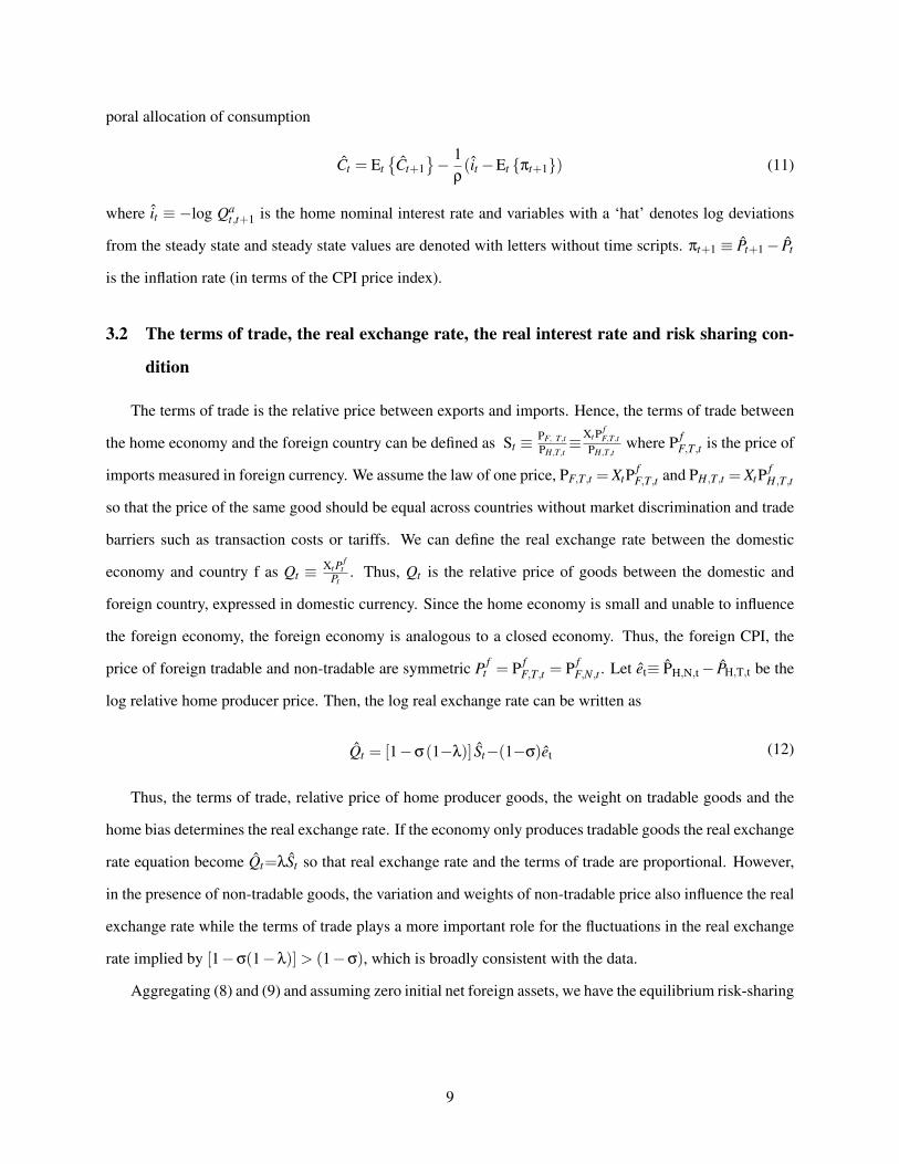
poral allocation of consumption

Ct = Et

Ct+1− 1

ρ(it −Et πt+1) (11)

where it ≡ −log Qat,t+1 is the home nominal interest rate and variables with a ‘hat’ denotes log deviations

from the steady state and steady state values are denoted with letters without time scripts. πt+1 ≡ Pt+1− Pt

is the inflation rate (in terms of the CPI price index).

3.2 The terms of trade, the real exchange rate, the real interest rate and risk sharing con-

dition

The terms of trade is the relative price between exports and imports. Hence, the terms of trade between

the home economy and the foreign country can be defined as St ≡ PF, T,tPH,T,t≡Xt P

fF,T,t

PH,T,twhere P f

F,T,t is the price of

imports measured in foreign currency. We assume the law of one price, PF,T,t = XtPfF,T,t and PH,T,t = XtP

fH,T,t

so that the price of the same good should be equal across countries without market discrimination and trade

barriers such as transaction costs or tariffs. We can define the real exchange rate between the domestic

economy and country f as Qt ≡ Xt Pf

tPt

. Thus, Qt is the relative price of goods between the domestic and

foreign country, expressed in domestic currency. Since the home economy is small and unable to influence

the foreign economy, the foreign economy is analogous to a closed economy. Thus, the foreign CPI, the

price of foreign tradable and non-tradable are symmetric P ft = P f

F,T,t = P fF,N,t . Let et≡ PH,N,t− PH,T,t be the

log relative home producer price. Then, the log real exchange rate can be written as

Qt = [1−σ(1−λ)] St−(1−σ)et (12)

Thus, the terms of trade, relative price of home producer goods, the weight on tradable goods and the

home bias determines the real exchange rate. If the economy only produces tradable goods the real exchange

rate equation become Qt=λSt so that real exchange rate and the terms of trade are proportional. However,

in the presence of non-tradable goods, the variation and weights of non-tradable price also influence the real

exchange rate while the terms of trade plays a more important role for the fluctuations in the real exchange

rate implied by [1−σ(1−λ)]> (1−σ), which is broadly consistent with the data.

Aggregating (8) and (9) and assuming zero initial net foreign assets, we have the equilibrium risk-sharing

9

condition

Ct −C ft = (

1ρ)Qt

= (1ρ)[[1−σ(1−λ)] St−(1−σ)et

] (13)

Risk sharing implies that since households purchase contingent claims, idiosyncratic shocks can be

insured away. Thus, the marginal utility of consumption of both countries, weighted by the real exchange

rate should be equalized, as noted by Backus & Smith (1993). While an increase in the price of non-tradable

goods reduces consumption through a higher relative price of home producer goods for given prices of

foreign and home tradable goods, lower consumption induced by an increase in the price of home tradable

goods through an appreciation of the terms of trade partially offset by a fall in the relative price of home

producer goods.

We define the Fisher equation as 1+ it ≡(

Pt+1Pt

)Rt and 1+ i f

t ≡(

P ft+1

P ft

)R f

t where Rt and R ft are the

home and foreign gross real interest rate. Combining with the uncovered interest parity condition under the

assumption of complete international financial markets , it = i ft +Et(4Xt+1) and log linearizing yields

Rt = R ft +Et(4Qt+1) (14)

Thus, the real interest rate depends on the foreign real interest rate and expected fluctuations of the

real exchange rate. Since the real exchange rate is influenced by prices of final non-tradable goods, final

non-tradable sectors have a critical role for the real interest rate.

3.3 Firms

As explained earlier, in our model, markets are segmented so that we have three sectors; final non-

tradable sectors, final tradable sectors and intermediate sectors. While final non-tradable sectors use labour

only for production, final tradable sectors use both labour inputs and intermediate inputs (home tradable and

non-tradable intermediate inputs and foreign tradable intermediate inputs). Final tradable sectors are mainly

manufacturing and final non-tradable sectors are mainly services which are consumed by households such

as education and housing. We assume that firms across different sectors are monopolistically competitive

and follow Calvo type sticky price setting in order to allow the same speed of adjustment in response to

stochastic shocks. Final domestic firms are indexed by z ∈ [0,λσ; λiσi,σi; σ,1] where [0,λσ; λiσi,σi]

represents final tradable firms producing goods for home and foreign consumers and [σ,1] represent firms

10

in non-tradable sectors.

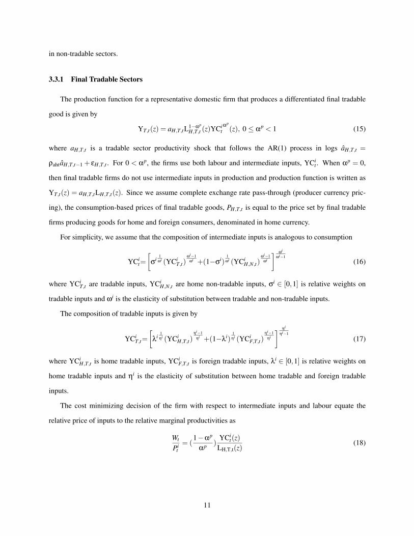
3.3.1 Final Tradable Sectors

The production function for a representative domestic firm that produces a differentiated final tradable

good is given by

YT,t(z) = aH,T,tL1−αp

H,T,t (z)YCitαp

(z), 0 ≤ αp < 1 (15)

where aH,T,t is a tradable sector productivity shock that follows the AR(1) process in logs aH,T,t =

ρahtaH,T,t−1 + εH,T,t . For 0 < αp, the firms use both labour and intermediate inputs, YCit . When αp = 0,

then final tradable firms do not use intermediate inputs in production and production function is written as

YT,t(z) = aH,T,tLH,T,t(z). Since we assume complete exchange rate pass-through (producer currency pric-

ing), the consumption-based prices of final tradable goods, PH,T,t is equal to the price set by final tradable

firms producing goods for home and foreign consumers, denominated in home currency.

For simplicity, we assume that the composition of intermediate inputs is analogous to consumption

YCit=

[σ

i1

ωi (YCiT,t)

ωi−1ωi +(1−σ

i)1

ωi (YCiH,N,t)

ωi−1ωi

] ωi

ωi−1(16)

where YCiT,t are tradable inputs, YCi

H,N,t are home non-tradable inputs, σi ∈ [0,1] is relative weights on

tradable inputs and ωi is the elasticity of substitution between tradable and non-tradable inputs.

The composition of tradable inputs is given by

YCiT,t=

[λ

i1ηi (YCi

H,T,t)ηi−1

ηi +(1−λi)

1ηi (YCi

F,T,t)ηi−1

ηi

] ηi

ηi−1

(17)

where YCiH,T,t is home tradable inputs, YCi

F,T,t is foreign tradable inputs, λi ∈ [0,1] is relative weights on

home tradable inputs and ηi is the elasticity of substitution between home tradable and foreign tradable

inputs.

The cost minimizing decision of the firm with respect to intermediate inputs and labour equate the

relative price of inputs to the relative marginal productivities as

Wt

Pit= (

1−αp

αp )YCi

t(z)LH,T,t(z)

(18)

11

where Pit is price of the aggregate input. The real marginal cost of producing final goods is given by

MCH,T,t =WtLαp

H,T,t(z)YCit−αp

(z)

(1−αp)aH,T,tPH,T,t(19)

Log linearizing around the steady state yields

MCH,T,t = Wt − PH,T,t− aH,T,t +αp(LH,T,t(z)− YC

it(z))

= (1−αp)W t− PH,T,t− aH,T,t +α

pPit

(20)

Thus, real marginal cost in terms of the price of tradable goods is common across the domestic firms

that produce final tradable goods. While an increase in wage and input costs increase real marginal costs, an

increase in the productivity reduces costs.

Due to analogous cost minimizing decisions, demand for each inputs yields

YCiH,T,t=λ

iσ

i

[Pi

H,T,t

PiT,t

]−ηi[Pi

T,t

Pit

]−ωi

YCit (21)

YCiF,T,t=(1−λ

i)σi

[Pi

F,T,t

PiT,t

]−ηi[Pi

T,t

Pit

]−ωi

YCit (22)

YCiH,N,t=(1−σ

i)

[Pi

H,N,t

Pit

]−ωi

YCit (23)

where PiT,t , Pi

H,T,t and PiH,N,t are the prices of tradable inputs, home tradable inputs and home non-tradable

inputs. The terms of trade in intermediate sectors is the relative price between intermediate exports and

imports and defined as Sit ≡

PiF,T,t

PiH,T,t

. Analogous to the final goods sectors, we assume the law of one price in

intermediate sectors.

A randomly selected proportion 1−θ of home tradable firms sets new prices each period while a fraction

θ keep their prices unchanged following the Calvo (1983) framework. The firms who can set new prices

each period maximize the expected present discounted profits, given by.

max∞

∑k=0

(θβ)kEt [YT,t+kPH,T,t −TCnH,T,t+k(YT,t+k)] (24)

subject to the sequence of demand functions YT,t+k ≤(

PH,T,tPH,T,t+k

)−ε

[( 1

λσ

)εCH,T,t+k +

(1

(1−λ f )σ f

)ε

C fH,T,t+k]

where TCnH,T,t+k is the nominal total cost of producing final tradable goods, PH,T,t is the prices set by firms

adjusting their prices in period t and YT,t+k is the corresponding output in period t + k.

12

The first order condition yields

∞

∑k=0

(βθ)kEt

YT,t+k(PH,T,t −ΨMCH,T,t+kPH,T,t+k

)= 0 (25)

where Ψ≡ ε

ε−1 is the markup of price over marginal cost in steady-state. The optimal price setting strategy

for firms setting a new price,PH,T,t in terms of the logs of nominal marginal costs MCnt is given by

PH,T,t = µ+(1−βθ)∞

∑k=0

(βθ)kEtMCnH,T,t+k (26)

where letters with tilde denote the logs of the respective variables and µ ≡ log ε

ε−1 is the logs of markup

of price over marginal cost in steady-state. The domestic tradable goods price index is given by

PH,T,t=[θ(PH,T,t−1)

1−ε+(1−θ)(PH,T,t)1−ε] 1

1−ε

, which, when log linearized around the zero inflation steady

state yields πH,T,t = (1−θ)(PH,T,t− PH,T,t−1). Combining this with the log linearized optimal price setting

strategy around the steady state, we have the marginal cost based domestic tradable inflation

πH,T,t = βEt(πH,T,t+1)+νMCH,T,t (27)

where ν≡ (1−βθ)(1−θ)

θ

3.3.2 Final Non-Tradable Sectors and Intermediate Sectors

We assume that the final non-tradable sectors and intermediate sectors have symmetric production func-

tions and Calvo-type sticky price setting decisions. Thus, firms use only labour inputs in production.

The production function for a representative domestic firm that produces a differentiated non-tradable

good is given by

YH,N,t (z) = aH,N,tLH,N,t (z) (28)

where aH,N,t is a non-tradable goods producing sector productivity shock that follows the AR(1) process in

logs.

The optimal decision of the firm yield the labour demand

MCH,N,t =Wt

PH,N,taH,N,t(29)

where MCH,N,t is real marginal cost of producing non-tradable goods in terms of the price of non-tradable

goods. Since we assume perfect labour mobility across sectors, workers in different sectors receive identical

13

wages.

Log linearizing around the steady state gives

MCH,N,t = Wt− PH,N,t− aH,N,t (30)

We assume intermediate tradable and non-tradable sectors are analogous to the final non-tradable sector

so that the production function is

YiT,t(z

i) = aH,T,tLiH,T,t(z

i); YiH,N,t(z

i) = aH,N,tLiH,N,t(z

i) (31)

where LiH,T,t is employment in home tradable input sectors and Li

H,T,t is employment in home non-tradable

input sectors. Price setting is analogous to (26) and the intermediate sector market clearing condition is

analogous to the final goods market clearing condition.

3.4 The New Keynesian Philips Curve

Log linearizing (4) and (5) around the steady state yields Pt = σPT,t +(1−σ)PH,N,t and PT,t = λPH,T,t +

(1− λ)PF,T,t. Combining with the terms of trade, domestic tradable and non-tradable inflation yields the

marginal cost and the terms of trade based New Keynesian Philips curve

πt = σπH,T,t +(1−σ)πH,N,t +σ(1−λ)∆St

= σ[βEt(πH,T,t+1)+νMCH,T,t ]+ (1−σ) [βEt(πH,T,t+1)+νMCH,T,t ]+σ(1−λ)∆St

= βEt πt+1+ν[σMCH,T,t+(1−σ)MCH,N,t ]−σ(1−λ)(β∆St+1− ∆St)

(32)

Thus, expected future inflation, an increase in marginal costs of both sectors and expected future ap-

preciation of the terms of trade generates current inflation. While an increase in marginal costs push up

production cost and thereby generates inflation, expected future appreciation of the terms of trade implies a

current depreciation under the assumption of trade balance in the long run and thus raises current inflation.

3.5 Consumption, Exports, Imports and Net Exports

We assume that households are identical within each country. The aggregate consumption of home

households, Ct = CH,T,t +CF,T,t +CH,N,t consists of demand for home tradable goods, imports from the

foreign country and home non-tradable goods. We assume the trade balance in the steady state CF,T = CfH,T

where steady state variables are denoted without time scripts so that in the steady state CH,T = Cλσ, CF,T =

14

CfH,T = C(1−λ)σ and CH,N = C(1−σ). Log linearizing the aggregate consumption around the steady state

yields

Ct = σλCH,T,t +σ(1−λ)CF,T,t +(1−σ)CH,N,t (33)

Foreign consumption of home tradable goods CfH,T,t=(1−λ f )σ f

[Pf

H,T,t

PfT,t

]−η[Pf

T,t

Pft

]−ω

Cft represents the de-

mand for exports to the foreign country. Log linearizing yields

EX t = ηSt +C ft (34)

where EX t is log linearized demand for exports. An increase in the terms of trade, allowing higher relative

foreign price, and higher elasticity of substitution between foreign and home tradable goods raises home

exports.

Consumption of foreign tradable goods, CF,T,t = (1−λ)σ[

PF,T,tPT,t

]−η[PT,tPt

]−ω

Ct represents the demand for

imports from the foreign country and combining with the risk sharing condition and log linearizing yields

IMt = Λet−ϒSt +C ft (35)

where Λ≡[ω−(1/ρ)] (1−σ) , ϒ≡(1−λ)

[ω(1−σ)+

(1ρ

)σ

]+λη−

(1ρ

)>0 and IMt is log linearized

imports. The demand for imports from the foreign country depends on the relative home producer price

and the terms of trade for given foreign consumption. Firstly, note that while depreciation of the terms

of trade unambiguously reduces imports, the impact of the relative home producer price depends on the

relative parameter values. When ω > (1/ρ), the expenditure switching effect between home non-tradable

goods and imports dominate the (state contingent) income effects induced by changes in purchasing power.

While an increase in the price of non-tradable goods leads to a switching of consumption from non-

tradable goods to imports, appreciation of the real exchange rate due to the higher aggregate price level

reduces aggregate consumption including imports and partially offsets the switching effect. The reverse

is true if ω < (1/ρ). When we do not have non-traded sectors, the demand for imports equation rep-

resents the substitution between home and foreign tradables EWT t = −[λ(η− 1ρ)]St + c f

t so that coupled

with the substitution between home and foreign tradable consumption, we observe additional substitu-

tion between consumption of home non-tradable goods and foreign tradable goods that is captured by

EWNt = Λet −[(1−σ)(1−λ)(ω−

(1ρ

))]

St. Thus, imports can be rewritten in terms of expenditure

15

switching between different varieties

IMt = EWT t + EWNt (36)

Combining the risk sharing condition and log linearizing net exports of final goods, NXt≡CfH,T,t −

PF,T,tPH,T,t

CF,T,t around the steady state yields

NX t = ξSt−Θet (37)

where ξ≡ σ(1−λ)

η−1+(1−λ)[ω(1−σ)+

(1ρ

)σ

]+λη−

(1ρ

)> 0 and

Θ≡ σ(1−λ)(1−σ) [ω−(

1ρ

)]. A higher (lower) degree of foreign (home) openness or a depreciation of the

terms of trade improve the trade balance while the impact of the relative home producer price depends on

the relative parameter values. An economy without a trade imblance is extensively discussed in the literature

by Obstfeld & Rogoff (1995), Benigno & Benigno (2003), Gali & Monacelli (2005) and De Paoli (2009)

among others; they show that under the assumption of η=ρ= 1, the economy never experiences a trade im-

balance. However, in the presence of non-tradable goods, the trade imbalance condition requires additional

assumptions. Thus, if η=ρ=ω= 1, the economy never experiences a trade imbalance. An increase in the

price of imports (foreign tradable goods) proportionally leads to the substitution towards home tradable and

non-tradable goods.

Log linearizing relative net exports,Cf

H,T,tCF,T,t

yields

RNX t = (Cft −Ct)−ω(1−σ) et +[η+λη+ω(1−σ)−λω(1−σ)]St

= (Cft −Ct)−ω(1−σ) et +υSt

= δSt−Λet

(38)

where υ≡ η+λη+ω(1−σ)−λω(1−σ) and

δ ≡ [(

1ρ

)[σ(1−λ)−1]+η+λη+ω(1−σ)−λω(1−σ)] > 0 so that an increase in the terms of trade in-

creases relative net exports.

16

3.6 Aggregate Demand

Since home tradable goods are consumed by home and foreign households, log linearizing demand for

the goods around the steady state with balanced trade and the market clearing condition6 yields

Yt = σλCH,T,t +σ(1−λ)CfH,T,t +(1−σ)CH,N,t (39)

We can find the links between domestic output and consumption by combining (33) and (39)

Yt = Ct +σ(1−λ) RNX t

= Ct +σ(1−λ)Cft +σ(1−λ)ηSt −σ(1−λ)(EWT t + EWNt)

= Ct +ϖQt +ΞSt

(40)

where ϖ≡[σ(1−λ)(

ω− 1ρ

)] and Ξ≡σ(1−λ) [η+λ(η−ω)]> 0. Thus, the discrepancy between demand

for home goods and consumption of home households arises from exports and imports. Home output in-

creases due to higher consumption and relative net exports.

Combining this with the risk sharing condition and foreign economy market clearing condition Yft = Cf

t7

yields aggregate demand

Yt = Cft +σ(1−λ) RNX t +(

1ρ)Qt

= Cft [1+σ(1−λ)]+σ(1−λ)ηSt −σ(1−λ)(EWT t + EWNt)+(

1ρ)Qt

= Cft +ΓQt +ΞSt

= Y ft +µSt − τet

(41)

where Γ≡ ϖ+ 1ρ> 0, µ≡Γ [1−σ(1−λ)]+Ξ> 0 and

τ≡Γ(1−σ)>0. This shows a spillover effect from the foreign country since foreign consumption raises

the demand for the domestic goods and so increases domestic output. Depreciation in the real exchange

generates an income effect raising home consumption and in turn, raising home output. Also, relative net

exports influence home output so that if exports are larger than imports, home production will increase

6We have three goods market clearing condition; market clearing condition for aggregate final goods, Yt = CH,T,t +CfH,T,t +

CH,N,t, for final tradable goods, YH,T,t = CH,T,t+CfH,T,t and for final non-tradable goods,YH,N,t = CH,N,t. Since intermediate sectors

also require labour, labour market clearing condition can be shown to be Lt = LH,T,t +LH,N,t +LiH,T,t +Li

H,N,t7Since the foreign country is assumed to be large, the home country is not able to influence foreign aggregate consumption,

interest rate and price level, and tradable sector becomes negligible. Thus, the foreign country is analogous to the closed economyand equilibrium condition yields Y f

t =Cft

17

and this influence is amplified with higher openness and weights on tradable consumption. Relative net

exports depends on the terms of trade and the relative prices between home tradable and non-tradable goods.

This implies that we observe relative home producer price effects along with terms of trade effects in the

presence of non-tradable goods. In other words, the terms of trade and the relative home producer prices

influence relative net exports and the real exchange rate thereby influencing aggregate output and generating

an externality. In sum, aggregate output can be characterized by the spillover effects in consumption, income

effects, the terms of trade effects and the expenditure switching effects between different varieties where the

expenditure switching effects and income effects are influenced by relative home producer price effects.

3.7 The Real Value of Home Production

The real value of home production is given by

Vt =

(PH,T,tYT,t +PH,N,tYH,N,t

Pt

)Combining aggregate demand and log linearizing around the steady state yields

Vt = Ct + NX t

= Cft + NX t +(

1ρ)Qt

= Cft +ΓQt +iSt

= Cft +Γ [1−σ(1−λ)]+i St −Γ(1−σ)et

(42)

where i≡σ(1−λ) [η+λ(η−ω) −1] > 0. If η=ω = ρ = 1, we have Vt = Qt + Cft so that depreciation

of the real exchange rate has a proportional effect on the real value of production and thereby generating a

proportional effect on consumption without net export effects. Thus if we have PPP then stochastic shocks

do not influence the real value of production. This implies that under complete markets, although positive

real income effects do not influence on home consumption itself due to consumption insurance, real income

effects are indirectly reflected through the risk sharing condition.

Under the assumption of η > ω, which is consistent with empirical observations, an increase (decrease)

of the terms of trade (relative non tradable prices) always has a positive effect on real value of home produc-

tion under complete financial markets.

18

3.8 Optimal Monetary Policy

In this section, we show the dynamics of the small open economy in terms of the output gap, the relative

price gap, the net exports gap and the New Keynesian Philips curve, and compare with the small open econ-

omy without non-tradable sectors and net exports. Also, we define net exports externalities in the optimal

allocation and the optimal monetary policy following Benigno & Benigno (2003) and Gali & Monacelli

(2005). We characterize the optimal allocation in the small open economy in terms of social planner. In

order to generate tractability of derivation of the optimality monetary policy, we exclude intermediate input

sectors, αp→ 0 and assume common value of the risk aversion, ρ = 1. Thus, in contrast to Gali & Mona-

celli (2005), we do not impose balanced trade for all t and maintain open economy features in a tractable

way. Firstly, by combining (10), (13), (20), (30) and (40), log linearized marginal cost of tradable and

non-tradable goods can be rewritten as8

MCH,T,t = ϕYt + Y ft + St −ϕat − aH,T,t (43)

MCH,N,t = ϕYt + Y ft + St − et −ϕat − aH,N,t (44)

Due to the analogous production function of tradable and non-tradable sectors, the economy wide real

marginal cost, MCt = σMCH,T,t + (1−σ)MCH,N,t can be written as MCt = ϕYt + Y ft − (1+ϕ)at + St −

(1−σ)et . Analogously, the aggregate productivity shocks can be written as at = σaH,T,t +(1−σ)aH,N,t .

Then, rearranging this equation, we obtain Yt = (1/ϕ)[MCt +(1+ϕ)at−Y ft − St +(1−σ)et ] . By imposing

MCt =−℘which is optimal marginal cost in a flexible price economy, the natural level of output is

Y t = (1/ϕ)[−℘+(1+ϕ)at − Y ft −St +(1−σ)et ]

=−℘+(1+ϕ)at +(1−µ

µ)Y f

t −[τ−µ(1−σ)

µ]et

(45)

where ≡ µ/(1+ϕµ). By defining the gap of respective variables as Y gt ≡ Yt−Y t , the relation between real

marginal cost, the output gap, the relative price gap [Sgt − (1−σ)eg

t ] and the net exports gap can be shown

to be

MCt = ϕY gt +[Sg

t − (1−σ)egt ]

= (1+ϕ)Y gt −NXg

t

(46)

An identity of the relative producer price gap by relating the changes in domestic tradable inflation,

8We show the dynamics of main variables in terms of the logs of variables rather than the log deviation around the steady statein this section in order to represent the economy in terms of the output gap.

19

non-tradable inflation and the natural relative producer price is

egt ≡ eg

t−1−πH,T,t +πH,N,t−∆et (47)

We can rewrite the New Keynesian Philips curve in terms of CPI inflation, the output gap, the net exports

gap and the terms of trade by combining (32) and (46)

πt = βEt πt+1+ν(1+ϕ)Y gt −NXg

t ]−σ(1−λ)(β∆St+1− ∆St) (48)

Also, the New Keynesian Philips curve for domestic tradable and non-tradable sectors can be written as

πH,T,t = βEt(πH,T,t+1)+ν[ϕY gt +Sg

t ]; πH,N,t = βEt(πH,N,t+1)+ν[ϕY gt +Sg

t − egt ] (49)

Combining (11), (32), (40) and (45) yields the so-called dynamic IS equation for the small open economy

with tradable and non-tradable goods in terms of the output gap and net exports9.

Y gt = EtY g

t+1− ∆NX t+1− [it −σEtπH,T,t+1− (1−σ)EtπH,N,t+1−Rt ] (50)

where Rt ≡ [ τ−µ(1+σϕ)µ ]aH,T,t(1−ρaht)−[ τ+µϕ(1−σ)

µ ]aH,N,t(1−ρahn)+(1−µµ )∆Y

fis the natural real in-

terest rate in terms of domestic goods (tradable and non-tradable goods).

Social planner maximizes utility of households subject to the risk sharing condition, production function

and the goods market clearing condition. The optimal allocation implies constant employment

L = Ω1/1+ϕ (51)

where Ω≡ [1−σ(1−λ)]/(1+ϖ)[1−σ(1−λ)]+Ξ. In order to identify net exports externalities coupled

with the monopolistic distortions, we add an employment subsidy or tax for the tradable, ℑT,t and non-

tradable sectors, ℑN,t . Then, the optimal decision of tradable and non-tradable firms in a flexible price

equilibrium can be shown to be

(ε−1

ε) = (1−ℑT,t)ΩS1−µ

t eτt (at/aH,T,t); (

ε−1ε

) = (1−ℑN,t)ΩS1−µt eτ−1

t (at/aH,N,t) (52)

9In order to derive the IS equation, we use definitions of the natural level of relative prices and net exports, et = aH,T,t − aH,N,t ,St = ( 1

µ )(Y t − Y ft + τet) and NX t = σ(1−λ)(RNX t− St).

20

We obtain an employment subsidy for tradable and non-tradable sectors by rearranging these equations

ℑT,t = 1− (ε−1

ε)Sµ−1

t e−τt

Ω(aH,T,t/at); ℑN,t = 1− (

ε−1ε

)Sµ−1

t e1−τt

Ω(aH,N,t/at) (53)

Thus, the optimal flexible price allocation can be obtained by imposing a subsidy, which ensures optimal

marginal cost in a flexible price economy, in a way to eliminate both terms of trade and relative home

producer price effects. Since optimal subsidies lead to constant relative producer price for all t and NXt =

Sµ−1t , the subsidies effectively eliminate net exports externalities along with the monopolistic distortions.

In the open economy with only tradable goods where σ→1, aH,T,t = at and balanced trade for all t (i.e.,

ρ = η = ω = 1), the optimal allocation leads to constant employment L = λ1/1+ϕ and employment subsidy

(ε−1

ε) = (1−ℑ)λ so that for a given subsidy in place, strict domestic tradable inflation targeting is optimal

as implied by (27), (41), (46) and πH,T,t = βEt(πH,T,t+1)+ν(1+ϕ)Y gt . and the small open economy needs

to stabilize domestic tradable inflation as Clarida et al. (2001), Gali & Monacelli (2005), Faia & Monacelli

(2007) and De Paoli (2009) among others point out.

However, when we allow non-tradable sectors and net exports, we also need to stabilize non-tradable

inflation by eliminating net exports externalities and this in turn, leads to Y gt = Sg

t = egt = 0 as implied by

(27), (41) and (49). Thus, there is no trade-off between output gap, terms of trade gap and relative producer

price gap stabilization, and we achieve “divine coincidence” as emphasized by Gali & Monacelli (2005) and

Corsetti et al. (2010). The optimal policy implies

Y gt = Sg

t = egt = πH,T,t = πH,N,t = 0 (54)

and

πt = (1µ)(∆Y t −∆Y f

t + τ∆et) (55)

CPI inflation fluctuates according to the growth rate of the natural relative producer price and the differ-

ence between the growth rate of the natural output and foreign output10.

Following Rotemberg & Woodford (1999) and Galı (2009), we can derive a second order approximation

to the welfare losses of households. The welfare loss function as a fraction of steady state consumption is

10Under the specific values of ρ = η = ω = 1, we have trade balance for all t and CPI inflation can be written as [ σ(1−λ)1−σ(1−λ)

]∆Qtso that the relative price distortions which distort purchasing power of domestic households through changes in the growth rate ofthe natural real exchange rate without improvement of trade balance need to be removed

21

shown to be

WLF t =−∞

∑t=0

βt(

Ω

2) ε

ν[σπ

2H,T,t +(1−σ)π2

H,N,t]+ (1+ϕ)Y gt

2 (56)

Additional source of welfare losses arises from non-tradable sectors in terms of composite domestic

inflation. Notice that the presence of non-tradable sectors generates a trade-off between stabilizing tradable

inflation, non-tradable inflation and the output gap without the fiscal instruments. Thus, the optimal policy

inevitably needs to deviate from stabilizing the three variables.

Without optimal subsidies in place, the central bank which can resort to commitment will minimizes

(56) subject to (41), (47), (49), and (50). Then, optimality conditions11 imply

σπH,T,t +(1−σ)πH,N,t =−µ(1+ϕ)

ε(ϕµ+1)∆Y g

t (57)

Combining (49) and (57), domestic price yields

PH,t = κPH,t−1 +κβPH,t−1 +κν[Sgt − (1−σ)eg

t ] (58)

for all t where PH,t = [σPH,T,t +(1−σ)PH,N,t] and κ≡ [ µ(1+ϕ)µ(1+ϕ)(1+β)+ενϕ(1+µϕ) ]. Thus, the stationary solution

yields

PH,t− ςPH,t−1 =ςν

1− ςβ[Sg

t − (1−σ)egt ]

=ςν

1− ςβ[Y g

t −NXgt ]

(59)

for all t where ς≡ 1−√

1−4βκ2

2βκ.

Rather than stabilizing tradable and non-tradable inflation, the central bank now faces a trade-off be-

tween stabilizing composite domestic inflation and the output gap due to net exports externalities.

In the absence of net exports externalities (i.e., ρ = η = ω = 1), the output gap is equal to the relative

price gap, Y gt = [Sg

t − (1−σ)egt ] and composite domestic inflation can be written as πH,t = βEt(πH,t+1)+

ν(1+ϕ)Y gt . Thus, stabilizing composite domestic inflation for all t is the optimal policy by closing the

output gap and satisfying the stationary solution.

Y gt = [Sg

t − (1−σ)egt ] = πH,t = 0 (60)

11The optimality conditions are ν(ϕµ+1

µ)(λ1

t +λ2t ) = −Ω(1+ϕ)Y g

t and Ωε

ν(σπH,T,t +(1−σ)πH,N,t) = ∆λ1

t +∆λ2t where λ1

t

and λ2t are the sequence of Lagrange multipliers.

22

While the optimal policy implies it = Rt , it leads to an indeterminacy problem as shown by Blanchard

& Kahn (1980) and Bullard & Mitra (2002). Thus, the central bank can implement the optimal policy by

committing to a rule

it = Rt +ρππH,t +ρyYg

t (61)

where ν(1+ϕ)(ρπ−1)+ (1−β)ρy > 0. Since πH,t = Y gt = 0 in equilibrium, ρππH,t +ρyY

gt will disappear

and this in turn leads to it = Rt for all t.

Thus, in contrast to the close economy12 and the open economy without net exports, the central bank

additionally needs to eliminate net exports externalities arising from imperfect substitutability between trad-

able goods, non-tradable goods and imports. However, since composite domestic inflation is a major de-

terminant of net exports as implied by (46), (49) and (50), strict composite domestic inflation targeting is a

good approximation to the optimal policy.

4 A Numerical Analysis

4.1 Calibration

Since the literature has assumed two large economies and correspondingly, calibrated for large

economies, we use small open economy (Korean) data in order to calibrate our model. We use the share

of consumption of non-tradable goods in GDP, 0.42, the share of consumption of imports in GDP, 0.1, the

share of intermediate inputs in GDP, 0.5, the share of distribution servies in GDP, 0.13 and the share of in-

termediate imports in GDP, 0.2 in South Korea during 1990-2016 in order to set the weights on consumption

of tradable goods σ = 0.58, on consumption of imports 1−λ = 0.17, on demand for tradable intermediate

inputs σi = 0.74 and on demand for intermediate imports 1−λi = 0.5413. We follow the standard assump-

tion that final tradable firms demand fixed proportions of tradable and non-tradable intermediate inputs,

ωi = 0.001 (see, for example, Burstein et al. (2003), Corsetti et al. (2008) and Dotsey & Duarte (2008)).

The elasticity of substitution between home and foreign intermediate input is set ηi = 3.14 which is es-

12In the close economy with two sectors, market clearing condition, the output gap and the New Keynesian Philips curve can beshown as Yt = Ct , Y g

t =−(1−σ)egt and πt = βEt πt+1+ν(1+ϕ)Y g

t . There is no trade-off between stablizing composite inflation,the output gap and the relative price gap. Thus, strict composite inflation targeting is the optimal policy as emphasized by Aoki(2001).

13Firstly, steady state values of the share of each consumption in GDP pin down the values of α and σ . Then, steady state valuesof the share of intermediate inputs, the share of distribution servies and the share of intermediate imports in GDP subsequently pindown the values of αp, λi and σi

23

Table 1: Parameters

HouseholdsDiscount rate β 0.99Risk aversion ρ 1Relative weight on tradable goods in the final consumption(unless specified otherwise)

σ 0.58

Inverse elasticity of labour supply (unless specified otherwise) ϕ 3Degree of trade openness (unless specified otherwise) α 0.17Elast. of substitution CH,T and CF,T (unless specified otherwise) η 1.5Elast. of substitution CT and CH,N (unless specified otherwise) ω 0.74Elast. of substitution individual varieties(unless specified otherwise)

ε 6

FirmElast. of output with respect to intermediate inputs(unless specified otherwise)

αp 0.86

Degree of price stickiness (unless specified otherwise) θ 0.75Elast. of substitution YCi

H,T and YCiF,T ηi 3.14

Elast. of substitution YCiT and YCi

H,N ωi 0.001Relative weight on intermediate non-tradable inputs 1−σi 0.26Relative weight on home intermediate tradable input λi 0.46Share of intermediate input in GDP Y i/Y 0.5Share of intermediate imports in GDP YCi

F,T/Y 0.2Share of distribution services in GDP YCi

H,N/Y 0.13Monetary policy

Inflation coefficient of the Taylor rule ρπ 1.5Degree of interest rate smoothing ρi 0.8

timated by Kasahara & Rodrigue (2008). β is set equal to 0.99 and thus the steady state Euler equation

β= 1/R implies a riskless steady state annual return of approximately 4%. Following Mendoza (1995) and

Benigno & Thoenissen (2008), the elasticity of substitution between tradable and non-tradable goods is set

as ω= 0.74. The elasticities of substitution between home tradable and foreign tradable goods and between

same category are set η= 1.5 and ε= 6 respectively. The calibration assumes common values of the risk

aversion, ρ = 1 and the inverse (Frisch) labour supply elasticity ϕ = 3. The Calvo probability of not being

able to adjust price is set equal to 0.75 implying an average of four periods between price adjustment. The

elasticity of output with respect to intermediate inputs is set to be αp= 0.8614 in order to pin down the share

of intermediate input in GDP.

We estimate the stochastic properties of the exogenous driving processes, using US real GDP (the proxy

for foreign output), Korean tradable and non-tradable sector labour productivity (the proxies for tradable and

14The economy without intermediate input sectors, αp→0 and correspondingly, α→0.5 in order to ensure that the share ofimports in GDP is 0.3

24

non-tradable productivity) log de-trended data during 2001q1-2016q4 in order to calibrate the properties.

The estimates are given by

aH,T,t = 0.61(0.07)

aH,T,t−1 + εH,T,t ,σH,T = 0.0242

aH,N,t = 0.52(0.08)

aH,N,t−1 + εH,N,t ,σH,N = 0.0169

Y ft = 0.89

(0.04)Y f

t−1 + εft ,σ

f = 0.0054

with corr(σH,T ,σH,N) = 0.53, corr(σH,T ,σf ) = 0.48 and corr(σH,N ,σ

f ) = 0.23.

4.2 Evaluation of Monetary Rules

This section evaluates monetary policy rules by excluding intermediate input sectors, αp → 0. While

the central bank needs to set an interest rate which achieves the stationary solution, it is nearly implausible

to conduct the optimal policy in practice since it is difficult to monitor the natural levels. Thus, we evaluate

alternative monetary policy rules associated with welfare. We have four Taylor-type rules responding to

composite domestic inflation and CPI inflation, and a rule for the fixed exchange rate regime. Specifically,

the composite domestic inflation-based Taylor rule (DTR) and the CPI-based Taylor rule (CTR) follow

it = ρππH,t; it = ρππt (62)

CPI inflation can be rewritten as πt = πH,t+σ(1−λ)∆St so that under CTR, the central bank additionally

responds to changes in the terms of trade. As values of (1−λ) and σ raise, it responses more to the changes.

The augmented composite domestic inflation-based Taylor rule (ADT) and the augmented CPI-based

Taylor rule (ACT) allow partial adjustment

it = ρi it−1 +(1−ρi)ρππH,t; it = ρi it−1 +(1−ρi)ρππt (63)

The exchange rate peg (PEG) follows

Xt = 0 (64)

In this welfare analysis, the source of fluctuations are tradable productivity, non-tradable productivity,

foreign output and composite shocks15. In addition to monetary rules, we also report the welfare losses of

15While our interests are mainly focused on tradable and non-tradable shocks, we include foreign output and composite shocksin order to compare with a welfare analysis presented by Gali & Monacelli (2005) and consider correlated shocks

25

Table 2: Evalaution of Alternative Monetary Policy Rules

TS Productivity Shocks NTS Productivity ShocksOP DTR CTR ADT ACT PEG OP DTR CTR ADT ACT PEG

σ (πH,T) 0.13 0.57 0.51 0.5 0.52 0.54 0.08 0.17 0.12 0.11 0.11 0.13σ (πH,N) 0.2 0.32 0.22 0.19 0.21 0.24 0.12 0.33 0.29 0.3 0.3 0.32σ (Y g) 0.04 0.63 0.83 0.94 1.02 1.12 0.03 0.28 0.32 0.43 0.44 0.51σ (πH) 0.01 0.46 0.38 0.37 0.39 0.41 0.01 0.23 0.19 0.19 0.18 0.21σ (π) 0.45 0.4 0.23 0.19 0.21 0.25 0.18 0.21 0.15 0.14 0.13 0.17σ (RPg) 0.21 0.29 0.45 0.54 0.61 0.69 0.15 0.39 0.43 0.52 0.53 0.59WL 0.0053 0.0524 0.0432 0.0429 0.0475 0.054 0.0019 0.0132 0.0101 0.0111 0.0111 0.0136

Foreign Output Shocks Composite ShocksOP DTR CTR ADT ACT PEG OP DTR CTR ADT ACT PEG

σ (πH,T) 0 0.03 0.1 0.02 0.05 0.22 0.11 0.68 0.59 0.57 0.58 0.56σ (πH,N) 0 0.03 0.1 0.02 0.05 0.22 0.17 0.56 0.46 0.44 0.44 0.47σ (Y g) 0 0.01 0.14 0.03 0.04 0.39 0.04 0.82 0.98 1.23 1.29 1.33σ (πH) 0 0.03 0.1 0.02 0.05 0.22 0.01 0.62 0.52 0.5 0.51 0.5σ (π) 0.14 0.15 0.12 0.17 0.13 0.15 0.52 0.57 0.4 0.38 0.37 0.34σ (RPg) 0 0.01 0.12 0.03 0.03 0.32 0.18 0.6 0.73 0.94 0.98 1.04WL 0 0.0001 0.0022 0.0001 0.0005 0.0116 0.004 0.089 0.069 0.072 0.075 0.076

the optimal policy (OP) in order to provide a useful benchmark.

Table 2 reports the standard deviations of main variables and the average period welfare losses in re-

sponse to tradable productivity, non-tradable productivity, foreign output and composite shocks for the opti-

mal policy and alternative monetary policy rules. Surprising result is that ironically, since DTR moderately

stabilize composite domestic inflation under the conventional inflation coefficient, ρπ = 1.5, it allows more

volatile tradable, non-tradable and composite domestic inflation16, thereby generating the highest welfare

losses except for PEG by tradable productivity, non-tradable productivity and composite shocks. On the

other hand, ADT leads to the lowest welfare losses in response to tradable productivity shocks. The partial

adjustment of the interest rates of ADT reduces volatilities of tradable, non-tradable and composite domestic

inflation. For non-tradable productivity shocks, CTR outperforms other policy rules. As implied by (48) and

(50), CTR stabilizes the relative price gap which in turn reduces a volatility of the output gap, and composite

domestic inflation. While CTR and ADT symmetrically stabilize composite domestic inflation, CTR further

reduces a volatility of the relative price gap and obtains lower welfare losses.

Turning to foreign output shocks. DTR and ADT stablize the output gap and composite domestic infla-

16This feature is also shown in comparing between CTR and ACT in terms of CPI inflation volatility. Thus, the moderatestabilization of target inflation leads to a higher volatility than partial adjustment of the interest rates towards the target inflation.

26

0 0.2 0.4 0.6 0.8 10

0.02

0.04

0.06

0.08

0.1

0.12TS Productivity Shocks

0 0.2 0.4 0.6 0.8 10

0.005

0.01

0.015

0.02

0.025

0.03NTS Productivity Shocks

0 0.2 0.4 0.6 0.8 10

0.05

0.1

0.15

0.2Composite Shocks

0 0.2 0.4 0.6 0.8 10

0.02

0.04

0.06

0.08

0.1

0 0.2 0.4 0.6 0.8 10

0.05

0.1

0.15

OP DTR CTR ADT ACT PEG

0 0.2 0.4 0.6 0.8 10

0.05

0.1

0.15,

< <

, ,

<

Welfareloss

Welfareloss

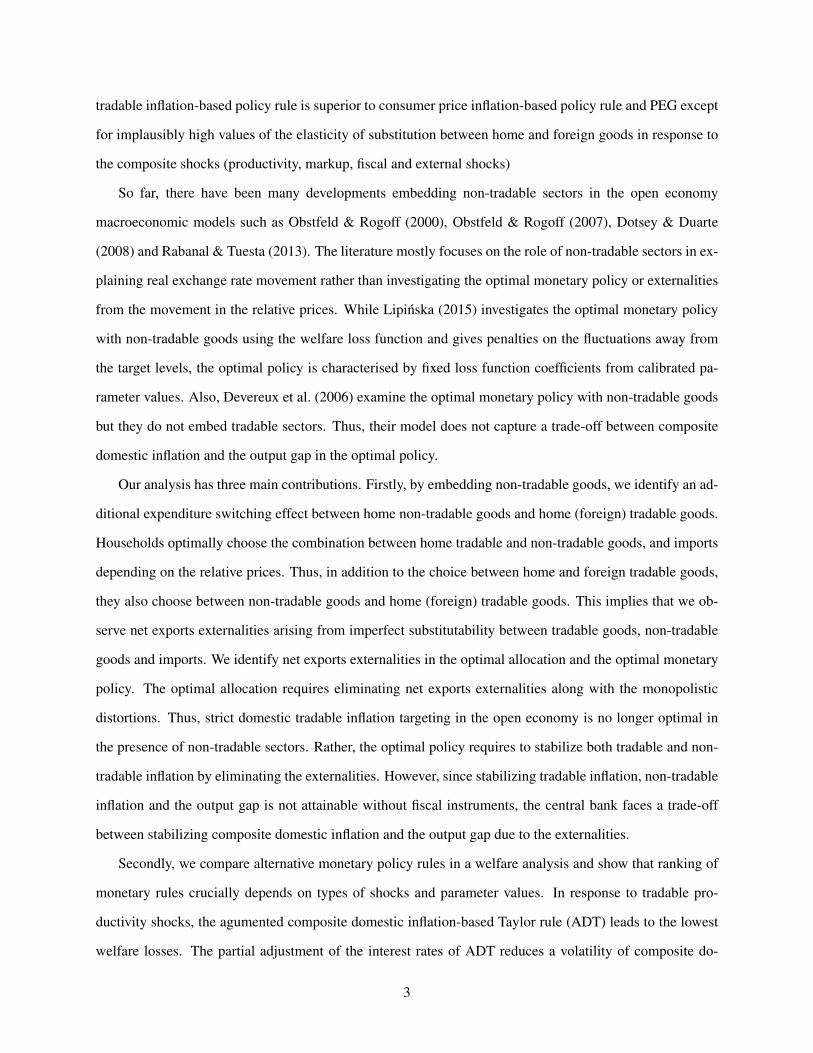
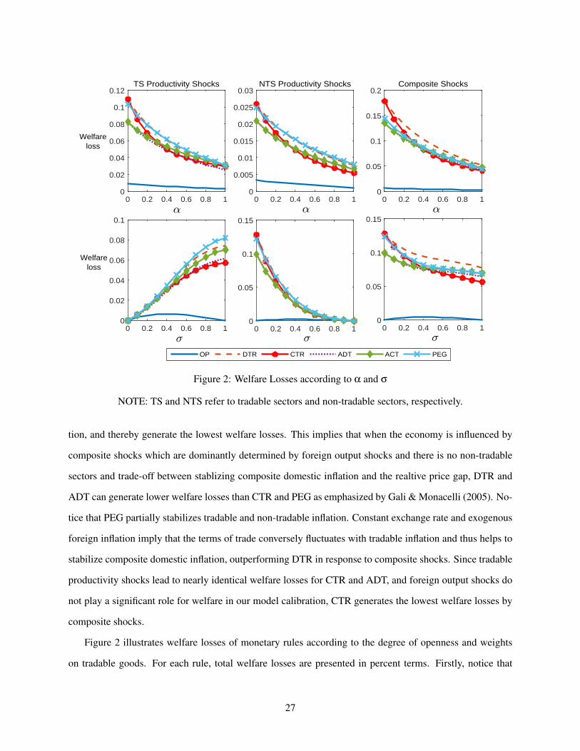
Figure 2: Welfare Losses according to α and σ

NOTE: TS and NTS refer to tradable sectors and non-tradable sectors, respectively.

tion, and thereby generate the lowest welfare losses. This implies that when the economy is influenced by

composite shocks which are dominantly determined by foreign output shocks and there is no non-tradable

sectors and trade-off between stablizing composite domestic inflation and the realtive price gap, DTR and

ADT can generate lower welfare losses than CTR and PEG as emphasized by Gali & Monacelli (2005). No-

tice that PEG partially stabilizes tradable and non-tradable inflation. Constant exchange rate and exogenous

foreign inflation imply that the terms of trade conversely fluctuates with tradable inflation and thus helps to

stabilize composite domestic inflation, outperforming DTR in response to composite shocks. Since tradable

productivity shocks lead to nearly identical welfare losses for CTR and ADT, and foreign output shocks do

not play a significant role for welfare in our model calibration, CTR generates the lowest welfare losses by

composite shocks.

Figure 2 illustrates welfare losses of monetary rules according to the degree of openness and weights

on tradable goods. For each rule, total welfare losses are presented in percent terms. Firstly, notice that

27

1 1.4 1.8 2.2 2.6 30

0.02

0.04

0.06

0.08TS Productivity Shocks

1 1.4 1.8 2.2 2.6 30

0.005

0.01

0.015

0.02NTS Productivity Shocks

1 1.4 1.8 2.2 2.6 30

0.05

0.1

0.15Composite Shocks

0 0.4 0.8 1.2 1.6 20

0.01

0.02

0.03

0.04

0.05

0.06

0 0.4 0.8 1.2 1.6 20

0.005

0.01

0.015

OP DTR CTR ADT ACT PEG

0 0.4 0.8 1.2 1.6 20

0.02

0.04

0.06

0.08

0.1

Welfareloss

! !!

22 2

Welfareloss

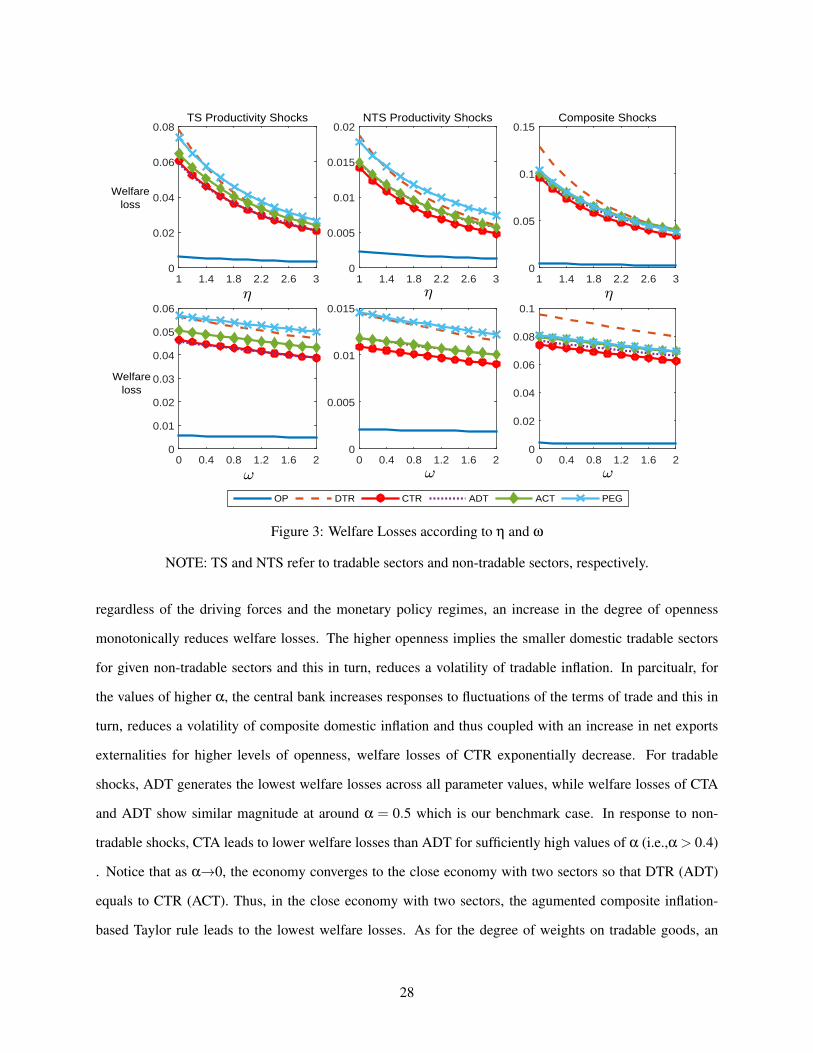
Figure 3: Welfare Losses according to η and ω

NOTE: TS and NTS refer to tradable sectors and non-tradable sectors, respectively.

regardless of the driving forces and the monetary policy regimes, an increase in the degree of openness

monotonically reduces welfare losses. The higher openness implies the smaller domestic tradable sectors

for given non-tradable sectors and this in turn, reduces a volatility of tradable inflation. In parcitualr, for

the values of higher α, the central bank increases responses to fluctuations of the terms of trade and this in

turn, reduces a volatility of composite domestic inflation and thus coupled with an increase in net exports

externalities for higher levels of openness, welfare losses of CTR exponentially decrease. For tradable

shocks, ADT generates the lowest welfare losses across all parameter values, while welfare losses of CTA

and ADT show similar magnitude at around α = 0.5 which is our benchmark case. In response to non-

tradable shocks, CTA leads to lower welfare losses than ADT for sufficiently high values of α (i.e.,α > 0.4)

. Notice that as α→0, the economy converges to the close economy with two sectors so that DTR (ADT)

equals to CTR (ACT). Thus, in the close economy with two sectors, the agumented composite inflation-

based Taylor rule leads to the lowest welfare losses. As for the degree of weights on tradable goods, an

28

increase in the weights on tradable (non-tradable) goods monotonically raises the welfare gap between

alternative policy rules due to a limited capability to control tradable (non-tradable) inflation of PEG and

an increase (decrease) in responses towards fluctuations of the terms of trade, along with an increase in net

exports externalities in response to tradable (non-tradable) shocks.

0.4 0.5 0.6 0.7 0.8 0.90

0.02

0.04

0.06

0.08TS Productivity Shocks

0.4 0.5 0.6 0.7 0.8 0.90

0.005

0.01

0.015NTS Productivity Shocks

0.4 0.5 0.6 0.7 0.8 0.90

0.02

0.04

0.06

0.08

0.1

0.12Composite Shocks

1.3 1.5 1.7 1.9 2.1 2.30

0.02

0.04

0.06

0.08

1.3 1.5 1.7 1.9 2.1 2.30

0.005

0.01

0.015

0.02

OP DTR CTR ADT ACT PEG

1.3 1.5 1.7 1.9 2.1 2.30

0.05

0.1

0.15

Welfareloss

Welfareloss

333

;:

;:

;:

Figure 4: Welfare Losses according to θ and ρπ

NOTE: TS and NTS refer to tradable sectors and non-tradable sectors, respectively.

Figure 3 represents welfare losses as a function of the elasticities of substitution between home tradable

and foreign tradable goods and between same category. Higher values of η and ω monotonically increase

the welfare gap between alternative policy rules except for DTR. The higher values imply a higher volatility

of the relative price gap and greater net exports externalities so that CTA increasingly dominates other policy

rules as the elasticities increase.

Figure 4 displays welfare losses in the plausible degree of price stickiness and the inflation coefficient

of the Taylor rule. For low price stickiness, DTR obtains the lowest welfare losses in response to tradable

productivity and composite shocks. However, when θ > 0.75, DTR leads to the highest welfare losses by

29

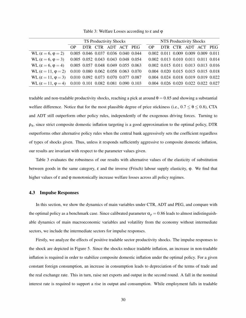
Table 3: Welfare Losses according to ε and ϕ

TS Productivity Shocks NTS Productivity ShocksOP DTR CTR ADT ACT PEG OP DTR CTR ADT ACT PEG

WL (ε = 6, ϕ = 2) 0.005 0.046 0.037 0.036 0.040 0.044 0.002 0.011 0.009 0.009 0.009 0.011WL (ε = 6, ϕ = 3) 0.005 0.052 0.043 0.043 0.048 0.054 0.002 0.013 0.010 0.011 0.011 0.014WL (ε = 6, ϕ = 4) 0.005 0.057 0.048 0.049 0.055 0.063 0.002 0.015 0.011 0.013 0.013 0.016WL (ε = 11, ϕ = 2) 0.010 0.080 0.062 0.058 0.063 0.070 0.004 0.020 0.015 0.015 0.015 0.018WL (ε = 11, ϕ = 3) 0.010 0.092 0.073 0.070 0.077 0.087 0.004 0.024 0.018 0.019 0.019 0.022WL (ε = 11, ϕ = 4) 0.010 0.101 0.082 0.081 0.090 0.103 0.004 0.026 0.020 0.022 0.022 0.027

tradable and non-tradable productivity shocks, reaching a pick at around θ = 0.85 and showing a substantial

welfare difference. Notice that for the most plausible degree of price stickiness (i.e., 0.7 ≤ θ ≤ 0.8), CTA

and ADT still outperform other policy rules, independently of the exogenous driving forces. Turning to

ρπ, since strict composite domestic inflation targeting is a good approximation to the optimal policy, DTR

outperforms other alternative policy rules when the central bank aggressively sets the coefficient regardless

of types of shocks given. Thus, unless it responds sufficiently aggressive to composite domestic inflation,

our results are invariant with respect to the parameter values given.

Table 3 evaluates the robustness of our results with alternative values of the elasticity of substitution

between goods in the same category, ε and the inverse (Frisch) labour supply elasticity, ϕ. We find that

higher values of ε and ϕ monotonically increase welfare losses across all policy regimes.

4.3 Impulse Responses

In this section, we show the dynamics of main variables under CTR, ADT and PEG, and compare with

the optimal policy as a benchmark case. Since calibrated parameter αp = 0.86 leads to almost indistinguish-

able dynamics of main macroeconomic variables and volatility from the economy without intermediate

sectors, we include the intermediate sectors for impulse responses.

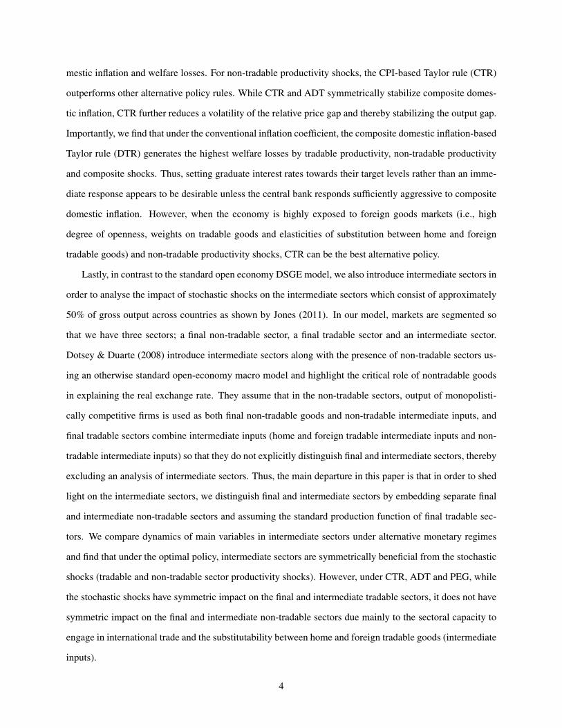
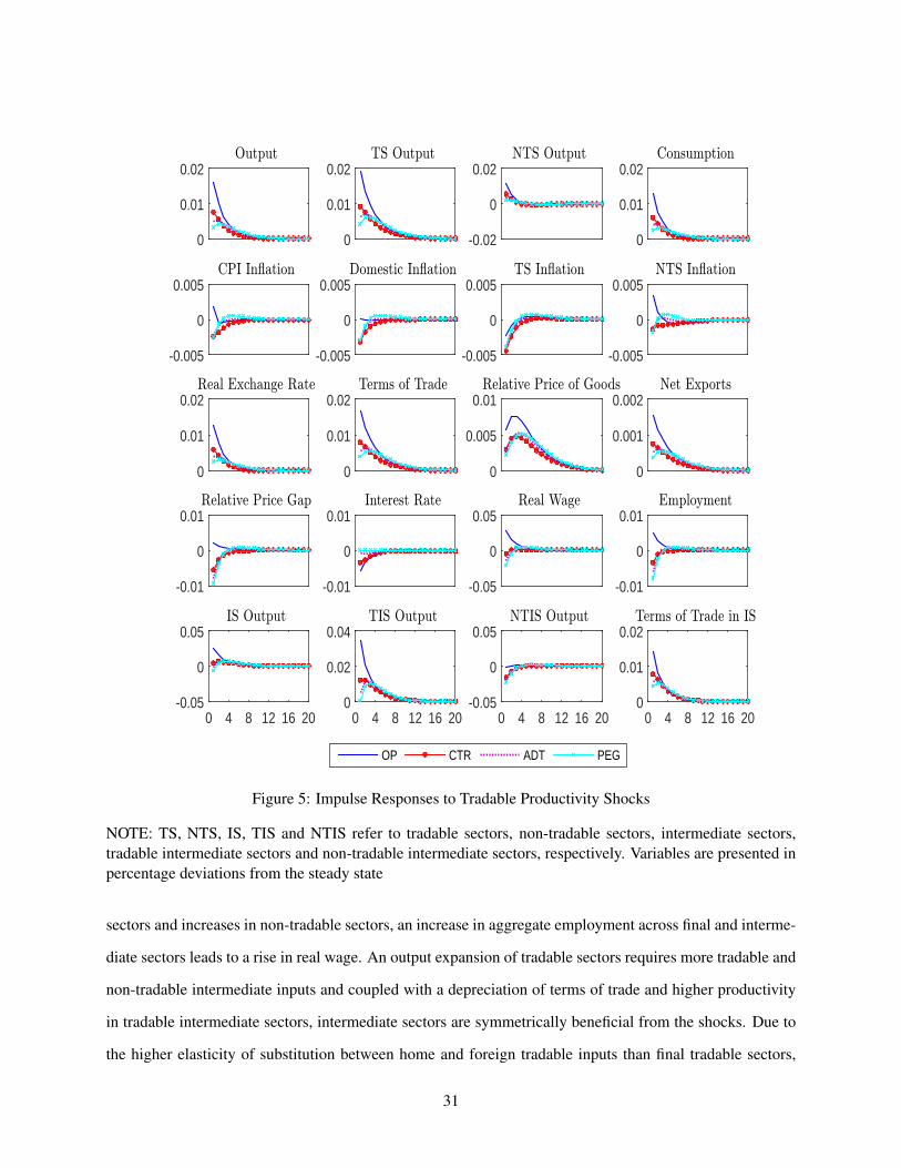
Firstly, we analyze the effects of positive tradable sector productivity shocks. The impulse responses to

the shock are depicted in Figure 5. Since the shocks reduce tradable inflation, an increase in non-tradable

inflation is required in order to stabilize composite domestic inflation under the optimal policy. For a given

constant foreign consumption, an increase in consumption leads to depreciation of the terms of trade and

the real exchange rate. This in turn, raise net exports and output in the second round. A fall in the nominal

interest rate is required to support a rise in output and consumption. While employment falls in tradable

30

0

0.01

0.02Output

0

0.01

0.02TS Output

-0.02

0

0.02NTS Output

0

0.01

0.02Consumption

-0.005

0

0.005CPI In.ation

-0.005

0

0.005Domestic In.ation

-0.005

0

0.005TS In.ation

-0.005

0

0.005NTS In.ation

0

0.01

0.02Real Exchange Rate

0

0.01

0.02Terms of Trade

0

0.005

0.01Relative Price of Goods

0

0.001

0.002Net Exports

-0.01

0

0.01Relative Price Gap

-0.01

0

0.01Interest Rate

-0.05

0

0.05Real Wage

-0.01

0

0.01Employment

0 4 8 12 16 20-0.05

0

0.05IS Output

0 4 8 12 16 200

0.02

0.04TIS Output

0 4 8 12 16 20-0.05

0

0.05NTIS Output

OP CTR ADT PEG

0 4 8 12 16 200

0.01

0.02Terms of Trade in IS

Figure 5: Impulse Responses to Tradable Productivity Shocks

NOTE: TS, NTS, IS, TIS and NTIS refer to tradable sectors, non-tradable sectors, intermediate sectors,tradable intermediate sectors and non-tradable intermediate sectors, respectively. Variables are presented inpercentage deviations from the steady state

sectors and increases in non-tradable sectors, an increase in aggregate employment across final and interme-

diate sectors leads to a rise in real wage. An output expansion of tradable sectors requires more tradable and

non-tradable intermediate inputs and coupled with a depreciation of terms of trade and higher productivity

in tradable intermediate sectors, intermediate sectors are symmetrically beneficial from the shocks. Due to

the higher elasticity of substitution between home and foreign tradable inputs than final tradable sectors,

31

output of tradable intermediate inputs further increases.

Turning to CTR, ADT and PEG. the productivity shocks also increase output of non-tradable sectors due

to an increase in aggregate consumption and the low elasticity of substitution between final tradable and non-

tradable sectors. In other words, while aggregate consumption and thus non-tradable consumption increase

due to the depreciation of the real exchange rate reflected in the risk sharing condition, the expenditure

switching effect between final tradable and non-tradable consumption partially offsets an increase in non-

tradable consumption. Since the shocks increase the relative price of home producer goods and the elasticity

of substitution is low, households moderately substitute from non-tradable goods to tradable goods. The

terms of trade and the real exchange rate depreciate and thus demand for exports increase and imports

decline which is reflected in higher net exports. Higher consumption coupled with higher net export leads

to a rise in the real value of home production. Final tradable firms demand fewer workers with higher

productivity so that a reduction of labour demand, reflected in lower wage and higher productivity reduces

marginal cost and this in turn, reduces domestic and CPI inflation. In contrast to PEG, ADT gradually

reduces the nominal interest rate and CTR immediately reduces the nominal interest rate in response to a

fall in composite domestic and CPI inflation, respectively. This in turn, increases consumption and output

further.

In intermediate input sectors, due to the higher productivity in tradable sectors (both final tradable and

tradable intermediate sectors), final tradable firms demand fewer intermediate inputs. However, the higher

productivity in tradable intermediate sectors implies lower prices of tradable intermediate inputs so that

analogous to final goods, the terms of trade in tradable intermediate sector depreciates and final tradable

firms substitute foreign intermediate inputs for home tradable intermediate inputs. This leads to a fall (rise)

in intermediate input imports (exports) and raises intermediate sector output. Thus, while final tradable

firms reduce demand for inputs which have fixed proportions of tradable and non-tradable intermediate

inputs, tradable intermediate sectors are positively influenced by the shock. Since non-tradable intermediate

firms are unable to engage in international trade, lower demand for intermediate inputs has a negative impact

on intermediate non-tradable sectors.

Figure 6 shows the impacts of positive non-tradable sector productivity shocks. Under the optimal

policy, the shocks lead to a fall in non-tradable inflation and correspondingly, a rise in tradable inflation as

expected. Since the shocks lead to depreciation of the terms of trade and the real exchange rate, net exports

increase and output increases symmetrically across different sectors.

32

-0.02

0

0.02Output

-0.02

0

0.02TS Output

0

0.01

0.02NTS Output

0

0.005

0.01Consumption

-0.002

0

0.002CPI In.ation

-0.005

0

0.005Domestic In.ation

-0.001

0

0.001TS In.ation

-0.005

0

0.005NTS In.ation

0

0.005

0.01Real Exchange Rate

-0.01

0

0.01Terms of Trade

-0.004

-0.002

0Relative Price of Goods

-0.001

0

0.001Net Exports

-0.01

0

0.01Relative Price Gap

-0.01

0

0.01Interest Rate

-0.05

0

0.05Real Wage

-0.01

0

0.01Employment

0 4 8 12 16 20-0.03

0

0.03IS Output

0 4 8 12 16 20-0.03

0

0.03TIS Output

OP CTR ADT PEG

0 4 8 12 16 20-0.02

0

0.02NTIS Output

0 4 8 12 16 20-0.01

0

0.01Terms of Trade in IS

Figure 6: Impulse Responses to Home Non-Tradable Productivity Shocks

NOTE: TS, NTS, IS, TIS and NTIS refer to tradable sectors, non-tradable sectors, intermediate sectors,tradable intermediate sectors and non-tradable intermediate sectors, respectively. Variables are presented inpercentage deviations from the steady state

With regard to alternative policy rules, while CTR, ADT and PEG show similar dynamics of the econ-

omy, CTR outperforms the others by immediately reducing the nominal interest rate in response to a fall

in CPI inflation and generating a lower response of the relative price gap, and PEG amplifies responses of

composite domestic inflation and the relative price gap due mainly to a very limited capability to gener-

ate depreciation of the terms of trade and the real exchange rate in response to the shocks. Under CTR,

33

ADT and PEG, the shocks reduce the marginal cost of producing final non-tradable goods and this leads

to depreciation (appreciation) of the terms of trade (relative home producer goods). Depreciation of the

real exchange rate due to changes of relative prices increases aggregate consumption as implied by the risk

sharing condition and output. With a lower price of non-tradable goods, households change their consump-

tion (domestic tradable and imports) towards non-tradable goods. While depreciation on the terms of trade

increases the real value of exports, an increase in the real value of imports due to the income effect which

dominates the expenditure switching effects (consumption of imports towards home non-tradable goods),

has a negligible impact on net exports. This implies that in response to the non-tradable productivity shocks,

output symmetrically fluctuates with consumption and the real exchange rate under complete financial mar-

kets. Turning to intermediate input sectors, since the shocks reduce the costs of non-tradable intermediate

inputs and thereby the marginal cost of final tradable firms and output, final tradable firms demand more

intermediate inputs for both tradable and non-tradable intermediate inputs due to fixed proportion of inputs’

demand, while tradable intermediate input sectors raise output further due to a depreciation of the terms

of trade in intermediate sectors. Thus, the shocks are symmetrically beneficial for final and intermediate

sectors.

5 Concluding Remarks

In this paper, we have extended a New Keynesian small open economy DSGE model with non-tradable

goods and intermediate inputs. We have investigated the optimal policy and evaluated alternative monetary

policy rules associated with welfare. Three main findings stand out.

Firstly, while the optimal policy requires stabilizing tradable inflation, non-tradable inflation and the

output gap by eliminating net exports externalities arising from imperfect substitutability between tradable

goods, non-tradable goods and imports, the optimal policy without fiscal instruments faces a trade-off be-

tween stabilizing composite domestic inflation and the output gap due to the externalities.

Secondly, ranking of alternative monetary policy rules crucially depends on types of shocks and param-

eter values. For tradable productivity shocks, the agumented composite domestic inflation-based Taylor rule

(ADT) outperforms other alternative policy rules by reducing a volatility of composite domestic inflation.

In response to non-tradable shocks, the CPI-based Taylor rule (CTR) leads to the lowest welfare losses by

additionally stabilizing the relative price gap and thereby reducing a volatility of the output gap. We find

34

that the composite domestic inflation-based Taylor rule (DTR) generates sizeable welfare losses under the

conventional inflation coefficient. Thus, setting graduate interest rates towards their target levels rather than

an immediate response appears to be desirable unless the central bank responds sufficiently aggressive to

composite domestic inflation. However, when the economy is highly exposed to foreign goods markets and

non-tradable productivity shocks, CTR can be the best alternative policy.

Thirdly, while final and intermediate sectors symmetrically beneficial from the stochastic shocks under

the optimal policy, asymmetric impact on different sectors arises under CTR, ADT and the exchange rate peg

(PEG) due mainly to the sectoral capacity to engage in international trade and the substitutability between

home and foreign tradable goods (intermediate inputs).

References

Aoki, K. (2001). Optimal monetary policy responses to relative-price changes. Journal of monetary eco-

nomics, 48, 55–80.

Backus, D. K., & Smith, G. W. (1993). Consumption and real exchange rates in dynamic economies with

non-traded goods. Journal of International Economics, 35, 297–316.

Benigno, G., & Benigno, P. (2003). Price stability in open economies. The Review of Economic Studies, 70,

743–764.

Benigno, G., & Thoenissen, C. (2008). Consumption and real exchange rates with incomplete markets and

non-traded goods. Journal of International Money and Finance, 27, 926–948.

Blanchard, O. J., & Kahn, C. M. (1980). The solution of linear difference models under rational expectations.

Econometrica, 48, 1305–1312.

Bullard, J., & Mitra, K. (2002). Learning about monetary policy rules. Journal of monetary economics, 49,

1105–1129.

Burstein, A., Eichenbaum, M., & Rebelo, S. (2005). Large devaluations and the real exchange rate. Journal

of Political Economy, 113, 742–784.

Burstein, A. T., Neves, J. C., & Rebelo, S. (2003). Distribution costs and real exchange rate dynamics during

exchange-rate-based stabilizations. Journal of monetary Economics, 50, 1189–1214.

35

Calvo, G. A. (1983). Staggered prices in a utility-maximizing framework. Journal of monetary Economics,

12, 383–398.

Clarida, R., Gali, J., & Gertler, M. (2001). Optimal monetary policy in open versus closed economies: An

integrated approach. The American Economic Review, 91, 248.

Corsetti, G., Dedola, L., & Leduc, S. (2008). International risk sharing and the transmission of productivity

shocks. The Review of Economic Studies, 75, 443–473.

Corsetti, G., Dedola, L., & Leduc, S. (2010). Optimal monetary policy in open economies. In B. M.

Friedman, & M. Woodford (Eds.), Handbook of Monetary Economics chapter 16. (pp. 861–933). Elsevier

volume 3.

Corsetti, G., & Pesenti, P. (2001). Welfare and macroeconomic interdependence. Quarterly Journal of

Economics, (pp. 421–445).

De Paoli, B. (2009). Monetary policy in a small open economy: the role of the asset market structure.

Journal of Money, Credit and Banking, 41.

Devereux, M. B., Lane, P. R., & Xu, J. (2006). Exchange rates and monetary policy in emerging market

economies. The Economic Journal, 116, 478–506.

Dotsey, M., & Duarte, M. (2008). Nontraded goods, market segmentation, and exchange rates. Journal of

Monetary Economics, 55, 1129–1142.

Faia, E., & Monacelli, T. (2007). Optimal interest rate rules, asset prices, and credit frictions. Journal of

Economic Dynamics and Control, 31, 3228–3254.

Galı, J. (2009). Monetary Policy, inflation, and the Business Cycle: An introduction to the new Keynesian

Framework. Princeton University Press.

Gali, J., & Monacelli, T. (2005). Monetary policy and exchange rate volatility in a small open economy.

The Review of Economic Studies, 72, 707–734.

Jones, C. I. (2011). Intermediate goods and weak links in the theory of economic development. American

Economic Journal: Macroeconomics, (pp. 1–28).

36

Kasahara, H., & Rodrigue, J. (2008). Does the use of imported intermediates increase productivity? plant-

level evidence. Journal of development economics, 87, 106–118.

Lipinska, A. (2015). Optimal monetary policy for the emu accession countries. a new keynesian approach.

Macroeconomic Dynamics, 19, 1427–1475.

Meier, S. (2013). Financial globalization and monetary transmission. Working Paper Swiss National Bank.

Mendoza, E. G. (1995). The terms of trade, the real exchange rate, and economic fluctuations. International

Economic Review, (pp. 101–137).

Obstfeld, M., & Rogoff, K. (1995). Exchange rate dynamics redux. Journal of Political Economy, (pp.

624–660).

Obstfeld, M., & Rogoff, K. (2000). Perspectives on oecd economic integration: implications for us current

account adjustment. Global Economic Integration: Opportunities and Challenges, (pp. 168–209).

Obstfeld, M., & Rogoff, K. (2007). The unsustainable us current account position revisited. In G7 current

account imbalances: Sustainability and adjustment (pp. 339–376). University of Chicago Press.

Rabanal, P., & Tuesta, V. (2013). Nontradable goods and the real exchange rate. Open Economies Review,

24, 495–535.

Rotemberg, J. J. (1982). Sticky prices in the united states. The Journal of Political Economy, (pp. 1187–

1211).

Rotemberg, J. J., & Woodford, M. (1999). Interest rate rules in an estimated sticky price model. In Monetary

policy rules (pp. 57–126). University of Chicago Press.

Stockman, A., & Tesar, L. (1995). Tastes and technology in a two-country model of the business cycle:

Explaining international comovements. American Economic Review, 85, 168–85.

Sutherland, A. (2005). Incomplete pass-through and the welfare effects of exchange rate variability. Journal

of international economics, 65, 375–399.

37