Monetary Policy Drivers of Bond and Equity Risks long stocks and short bonds)....Understanding...

Monetary Policy Drivers of Bond and Equity Risks

John Y. Campbell, Carolin Pflueger, and Luis M. Viceira

Harvard University, University of British Columbia, and HBS

March 2014

Campbell, Pflueger, and Viceira (2014) Bond and Equity Risks March 2014 1 / 34

Motivation Background

Changing Risks of Treasury Bonds

US Treasuries are viewed differently today:I “Inflation risk premium” in 1980sI “Anchor to windward”or "safe haven" in 2000s.

Treasuries comoved positively with stocks and the economy in the1980s, negatively in the 2000s.

Important implications for portfolio construction and asset pricing:I Bonds hedge stocks in endowment portfoliosI Equity investing is riskier for pension funds with fixed long-termliabilities

I Increased default risk for firms with long-term liabilitiesI Term premium and average yield spread are likely to be lower.

What has caused this change?1 Changes in monetary policy?2 Changes in macroeconomic shocks?



Changing Risks of Treasury Bonds

Over the past decade, the correlation of stocks and bonds has remainedpersistently negative (causing big problems for pension funds that areessentially long stocks and short bonds)....Understanding correlationsrequires an understanding of the nature and causes of asset returns.

Bridgewater Associates, LP, 2013, Recent Shifts in Correlations Reflect theDrivers of Markets, Bridgewater Daily Observations



Changing Beta of US Treasury Bonds


Motivation Our Contribution

This Paper

Model output gap, inflation, and policy rate in canonical NewKeynesian framework.

Endogenize bond and stock returns to match second moments:I Use habit formation and stochastic volatility of macro shocksI Combine modeling conventions of macroeconomics and asset pricing(while trying not to create a “mutant toy” that both fields dislike.)

Calibrate model to three monetary policy regimes.I Pre-Volcker (1960.Q1-1979.Q2): Accommodation of inflationI Volcker-Greenspan (1979.Q3-1996.Q4): Aggressive counter-inflationarypolicy (Clarida, Gali, and Gertler 1999)

I Increased Transparency (1997.Q1-2011.Q4): Monetary policypersistence and continued shocks to inflation target.


Motivation Literature

Related LiteratureEmpirical time-variation in bond risks: Baele, Bekart, andInghelbrecht (2010), Viceira (2012), David and Veronesi (2013), Campbell,Sunderam, and Viceira (2013), Kang and Pflueger (2013).Affi ne term structure models with macro factors: Ang and Piazzesi(2003), Ang, Dong, and Piazzesi (2007), Rudebusch and Wu (2007).Asset-pricing implications of real business cycle models: Bansaland Shaliastovich (2010), Buraschi and Jiltsov (2005), Burkhardt andHasseltoft (2012), Gallmeyer et al (2007), Piazzesi and Schneider (2006).Term-structure implications of New Keynesian models: Andreasen(2012), Bekaert, Cho and Moreno (2010), van Binsbergen et al. (2012),Kung (2013), Palomino (2012), Rudebusch and Wu (2008), Rudebusch andSwanson (2012).Monetary policy regime shifts: Clarida, Gali and Gertler (1999, 2000),Boivin and Giannoni (2006), Rudebusch and Wu (2007), Smith and Taylor(2009), Chib, Kang, and Ramamurthy (2010), Ang, Boivin, Dong, and Kung(2011), Bikbov and Chernov (2013).


Motivation Road Map

Road Map

A New Keynesian asset pricing model

Data

Estimating monetary policy rules in three regimes

Model calibration to three monetary regimes

Counterfactual analysis of bond and equity risks


Model Overview

Model Overview

“A standard New Keynesian model has emerged”(Blanchard and Gali2007):

I Euler equation is New Keynesian equivalent of Investment and Savings(IS) curve

I Phillips Curve (PC) with both forward-looking and backward-lookingcomponents captures nominal rigidities and productivity shocks

I Monetary Policy (MP) rule follows a Taylor (1993) rule withtime-varying inflation target.

Stochastic discount factor (SDF) with habit formation generatesEuler equation and prices stocks and bonds:

I Risk premia increase during recessions, consistent with the empiricalevidence on stock and bond return predictability (Fama and French1989).


Model Euler Equation (IS Curve)

SDF Implies Euler Equation

For SDF Mt+1 and gross real one-period asset return (1+ Rt+1),

1 = Et [Mt+1(1+ Rt+1)] .

Household optimization:

Mt+1 =βU ′t+1U ′t

.

Assuming no risk premia on short-term nominal interest rates:

it = rt + Etπt+1.

Euler equation for nominal T-bill (ignoring constants):

lnU ′t = (it − Etπt+1) + lnEtU ′t+1.



Modeling Marginal UtilityFor preference parameter α and heteroskedasticity parameter b > 0,assume analytically tractable form:

lnU ′t = −α(xt − θxt−1 − vt ) (1)

Vart (lnU ′t ) = α2σ2(1− bxt )Current and lagged output gap affect level of surplus consumption:

I Habit formation preferences of Campbell and Cochrane (1999) producedesired properties for SDF.

I Empirically plausible: Stochastically detrended log consumption andthe log output gap 90% correlated.

Output gap negatively affects volatility of surplus consumption andhence marginal utility:

I Countercyclical volatility of asset returnsI Countercyclical risk premiaI Campbell and Hentschel (1992), Calvet and Fisher (2007), Campbelland Beeler (2012), Bansal, Kiku and Yaron (2011), Bansal, Kiku,Shaliastovich, and Yaron (2014)



Output Gap and De-Trended Consumption

05

1015

Log

Det

rend

ed C

onsu

mpt

ion

(%)

10

50

510

Log

Out

put G

ap (%

)

60 70 80 90 00 10Year

Log Output Gap (%) Log Detrended Consumption (%)



Forward- and Backward-Looking Euler Equation

xt = ρx−xt−1 + ρx+Etxt+1 − ψ (it − Etπt+1) + uISt .

Forward- and backward-looking Euler equation captures thehump-shaped output gap response to shocks (Fuhrer 2000,Christiano, Eichenbaum, and Evans 2005).

Here ρx− = θ1+θ∗ , ρx+ = 1

1+θ∗ , ψ = 1α(1+θ∗) , θ∗ = θ − αbσ2/2 < θ.

Marginal utility shocks drive IS shocks: uISt =1

1+θ∗ vt .

Countercyclical shock volatility (b > 0) implies that ρx+ + ρx− > 1.


Model Phillips Curve

Forward- and Backward-Looking Phillips Curve

πt = ρππt−1 + (1− ρπ)Etπt+1 + λxt + uPCt

Calvo (1983) model of monopolistically competitive firms andstaggered price setting implies a forward-looking Phillips curve.

Infrequent information updating can give rise to backward-lookingPhillips curve (Mankiw and Reis 2002).

PC shock uPCt reflects productivity or cost-push shocks.


Model Monetary Policy Rule

Monetary Policy Rule

it = ρi (it−1 − π∗t−1) + (1− ρi ) [γxxt + γπ (πt − π∗t )] + π∗t + uMPt

π∗t = π∗t−1 + u∗t

Taylor (1993) rule with the Fed funds rate as policy instrument(Clarida, Gali, Gertler 1999, Rudebusch and Wu 2007).Fed funds rate adjusts gradually to target.Fed funds target increases in the output gap xt and the inflation gapπt − π∗t .Changes in central bank inflation target π∗t are unpredictable:

I Dynamics of π∗t consistent with persistent component in inflation andnominal interest rates (Ball and Cecchetti 1990, Stock and Watson2007).

I Persistent inflation target shifts term structure similar to a level factor(Rudebusch and Wu 2007, 2008).


Model Closing the Model

Summary of the Macro Model

xt = ρx−xt−1 + ρx+Et−xt+1 − ψ(Et−it − Et−πt+1) + uISt

πt = ρππt−1 + (1− ρπ)Et−πt+1 + λxt + uPCt

it = ρi (it−1 − π∗t−1) + (1− ρi ) [γxxt + γπ (πt − π∗t )] + π∗t + uMPt

π∗t = π∗t−1 + u∗t


Model Closing the Model

Stochastic Volatility for All Shocks

Independently and conditionally normal vector of shocks:

ut = [uISt , uPCt , uMPt , u∗t ]

′

Conditional variance-covariance matrix:

Σu (1− bxt−1) =

(σIS )2 0 0 00 (σPC )2 0 00 0 (σMP )2 00 0 0 (σ∗)2

(1− bxt−1) .Common stochastic volatility for all shocks makes model tractableand generates time-varying risk premia.


Model Modeling Bonds and Stocks

Modeling Bonds and Stocks

Solve for nominal bond returns using Campbell and Ammer (1993)exact loglinear return decomposition

r $n−1,t+1 − Et r $

n−1,t+1 = A$,nut+1.

Model stocks as levered claim on log output gap (Abel 1990,Campbell 1986, 2003): dt = δxt .

Solve for equity returns using Campbell and Shiller (1988) loglinearapproximation

r et+1 − Et r et+1 = Aeut+1.Solve for the nominal bond CAPM beta, and the volatilities of stockand bond excess returns.

I The model is ready to drive!


Data and Summary Statistics Monetary Policy Regimes

Monetary Policy Regimes

Divide sample in three subperiods:1 Pre-Volcker [1960.Q1-1979.Q2]2 Volcker - pre-1997 Greenspan [1979.Q3-1996.Q4]3 Post-1996 Greenspan - Bernanke [1997.Q1-2011.Q4]

Subperiods 1 and 2 identical to Clarida, Gali, and Gertler (1999)I Post-Volcker Federal Reserve counteracts inflation

Superiod 3 is newly identified in this paperI Increased transparency and gradualismI Publication of FOMC transcriptsI Not a single dissenting vote at FOMC meetings since 1997I Greenspan and Bernanke argue for cautious monetary policy in light ofincreased uncertainty about the effects of monetary policy

I Characterized by negative bond beta


Data and Summary Statistics Data

Data

GDP in 2005 chained dollars and GDP deflator from Bureau ofEconomic Analysis.

Potential output from Congressional Budget Offi ce.

Federal funds rate from Federal Reserve H.15 publication.

Five-year bond yield from CRSP Fama-Bliss data base.

Value-weighted NYSE/AMEX/Nasdaq stock return from CRSP.

S&P 500 dividend-price ratio from Robert Shiller’s web site.

Real consumption expenditures data for nondurables and servicesfrom the Bureau of Economic Analysis.


Data and Summary Statistics Data

Output Gap and Price-Dividend Ratio


Estimating Monetary Policy Rules


it = c0 + cxxt + cππt + c i it−1 + εt

ρi = c i , γx = cx/(1− c i ), γπ = cπ/(1− c i ).

Post-1979I γπ ↑ γx ↓I Stronger inflation responseI Weaker output response

Post-1997I ρi ↑I Stronger persistence


Model Calibration

Calibration ProcedureSpecify time-invariant vs. time-varying parameters to isolate effects ofchanging monetary policy and macroeconomic shocks (Smets andWouters, 2007):

I Time-varying parameters: Monetary policy rule parameters andvolatilities of shocks.

I Time-invariant parameters: ρ, δ, α, ρπ, ρx+, ρx−, λ.

Set monetary policy parameters to estimated values.Phillips curve parameters follow the literature: λ = 0.3 (Clarida, Gali,and Gertler, 1999) and ρπ = 0.8 (Fuhrer, 1997).Set leverage δ = 2.43 to match relative volatility of real dividendgrowth and real output gap growth, and utility curvature α = 30 tomatch equity volatility.Choose remaining parameters to minimize distance between modeland empirical moments:

I Slope coeffi cients and residual volatilities for a VAR(1) in log outputgap, inflation, Fed funds rate, and five-year nominal yield; volatilities ofbond and stock returns; and beta of bonds with stocks.


Model Calibration

Model and Empirical Moments


Counterfactual Analysis

Counterfactuals: MP Inflation Response and Persistence


Counterfactual Analysis Impulse Response Functions

Impulse Response Functions

Impulse responses are to one-standard deviation shocks

Units for the output gap and dividend-price ratio are in percentdeviations from the steady state.

Units for other variables are annualized percentage points.

60.Q1-79.Q2= blue solid, 79.Q3-96.Q4=green dash,97.Q4-11.Q4=red dash-dot.




MP shocks and IS shocks contribute essentially zero to bond beta

PC shock lowers output and raises inflation:I Stock prices fallI Effect on bond yields depends on monetary policy regimeI Creates a positive bond beta in the first two regimes, a negative one inthe third.

Inflation target shocks raise inflation and nominal interest ratesI Inflation below new target.I Central bank lowers real rates, creating a boom.I Bond prices fall and stock prices rise, creating a negative bond betaI When monetary policy is persistent, central bank does not lower realinterest rates immediately but only with a long lag. Stronger effect onbond yields and bond betas.



Why Changes not Driven by Volatilities?

Partial derivatives reveal that:I Model equity return volatility driven by PC shocks.I Model bond return volatility driven by inflation target shocks and PCshocks.

Empirical volatility of equity and bond returns changed little acrossregimes.

I Model matches this with near-constant PC and inflation target shockvolatilities.

I Changes in the volatility of shocks cannot explain changes in bond beta.I Point estimates even have opposite sign.



Important Amplification Channel: Risk Premia

Key role of time-varying volatility: higher risk premia duringrecessions.

Nominal bonds are hedges during third subperiod.I Bond hedging value especially valuable during recessions, when equityrisk premia are high.

I As a result, see negative bond yield response in response to PC shock.

Time-varying volatility also generates time-varying Jensen’s inequality(JI) effect.

I But JI term mostly level effect.I Generate plausible bond return volatility, so JI term unlikely to be toolarge.

I Do implications change if we ignore JI terms?



Counterfactuals: MP Inflation Response and Persistence



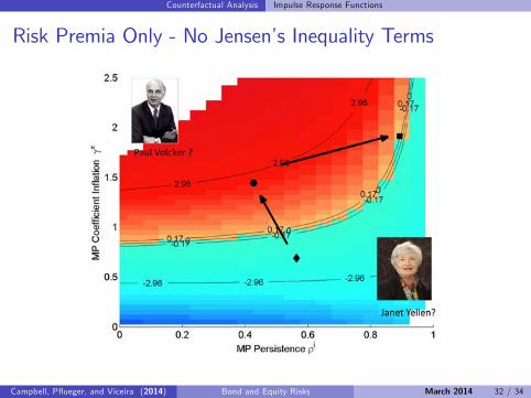
Risk Premia Only - No Jensen’s Inequality Terms


Conclusion

Conclusion

Fed anti-inflationary stance after 1979 increased nominal bond beta:I Large increase in Fed funds rate in response to inflation shockI Increase in Fed Funds rate depresses output, stock prices, and bondprices.

Persistent monetary policy (gradualism) and shocks to inflation targetgenerate negative nominal bond beta since mid 1990s:

I Inflation target shock decreases bond pricesI Real rates fall in response to inflation target shock, driving up outputand equity prices.

I Changes in offi cial central bank inflation target or central bankcredibility?

Phillips Curve (supply) shocks increase nominal bond beta, butmodest variation across regimes.

Changing risk premia offer important amplification mechanism.


Additional Slides

Unconditional Variances

Unconditional variance equals conditional variance at zero output gap

Var(r et+1 − Et r et+1) = E[AeΣuAe ′(1− bxt )

]= AeΣuAe ′.

Investors in our model use this analytic unconditional variance toprice bonds and stocks.

I Report analytic unconditional variances and covariances.

Conditional variances can and do turn negative in calibration.I Model-implied unconditional variances lower than in a model whereconditional variances truncated below at zero.

I Similar results for alternative calibration in which conditional variancesalmost never go negative.


Monetary Policy Drivers of Bond and Equity Risks long stocks and short bonds)....Understanding...

Documents

Transcript of Monetary Policy Drivers of Bond and Equity Risks long stocks and short bonds)....Understanding...