Monetary Economics, 2nd Edition
871
Transcript of Monetary Economics, 2nd Edition


Monetary Economics,2nd Edition
This successful text, now in its second edition, offers the most comprehensive overview ofmonetary economics and monetary policy currently available. It covers the microeconomic,macroeconomic and monetary policy components of the field. The author also integrates thepresentation of monetary theory with its heritage, stylized facts, empirical formulations andeconometric tests.
Major features of the new edition include:
• Stylized facts on money demand and supply, and the relationships between monetarypolicy, inflation, output and unemployment in the economy.
• Theories on money demand and supply, including precautionary and buffer stock models,and monetary aggregation.
• Cross-country comparison of central banking and monetary policy in the US, UK andCanada, as well as consideration of the special features of developing countries.
• Competing macroeconomic models of the Classical and Keynesian paradigms, alongwith a discussion of their validity and consistency with the stylized facts.
• Monetary growth theory and the distinct roles of money and financial institutions ineconomic growth in promoting endogenous growth.
• Excellent pedagogical features such as introductions, key concepts, end-of-chaptersummaries, and review and discussion questions.
This book will be of interest to teachers and students of monetary economics, money andbanking, macroeconomics and monetary policy. Instructors and students will welcome theclose integration between current theories, their heritage and their empirical validity.
Jagdish Handa is Professor of Economics at McGill University in Canada and has taughtmonetary economics and macroeconomics for over forty years.


Monetary Economics,2nd Edition
Jagdish Handa

First published 2000Second edition published 2009by Routledge2 Park Square, Milton Park, Abingdon, Oxon OX14 4RN
Simultaneously published in the USA and Canadaby Routledge270 Madison Ave, New York, NY 10016
Routledge is an imprint of the Taylor & Francis Group,an informa business
© 2000, 2009 Jagdish Handa
All rights reserved. No part of this book may be reprinted or reproduced or utilizedin any form or by any electronic, mechanical, or other means, now known orhereafter invented, including photocopying and recording, or in any informationstorage or retrieval system, without permission in writing from the publishers.
British Library Cataloguing in Publication DataA catalogue record for this book is availablefrom the British Library
Library of Congress Cataloging in Publication DataA catalog record for this book has been requested
ISBN 10: 0-415-77209-5 (hbk)ISBN 10: 0-415-77210-9 (pbk)ISBN 10: 0-203-89240-2 (ebk)
ISBN 13: 978-0-415-77209-9 (hbk)ISBN 13: 978-0-415-77210-5 (pbk)ISBN 13: 978-0-203-89240-4 (ebk)
This edition published in the Taylor & Francis e-Library, 2008.
“To purchase your own copy of this or any of Taylor & Francis or Routledge’scollection of thousands of eBooks please go to www.eBookstore.tandf.co.uk.”
ISBN 0-203-89240-2 Master e-book ISBN

To Sushma, Sunny and Rish


Contents
Preface xxvAcknowledgments xxviii
PARTI
Introduction and heritage 1
1. Introduction 3
1.1 What is money and what does it do? 51.1.1 Functions of money 51.1.2 Definitions of money 5
1.2 Money supply and money stock 61.3 Nominal versus the real value of money 71.4 Money and bond markets in monetary macroeconomics 71.5 A brief history of the definition of money 71.6 Practical definitions of money and related concepts 12
1.6.1 Monetary base and the monetary base multiplier 141.7 Interest rates versus money supply as the operating target
of monetary policy 151.8 Financial intermediaries and the creation of financial assets 151.9 Different modes of analysis of the economy 181.10 The classical paradigm: the classical group of
macroeconomic models 201.11 The Keynesian paradigm and the Keynesian set of
macroeconomic models 241.12 Which macro paradigm or model must one believe in? 261.13 Walras’s law 281.14 Monetary policy 281.15 Neutrality of money and of bonds 291.16 Definitions of monetary and fiscal policies 30
Conclusions 31Summary of critical conclusions 32Review and discussion questions 32References 33

viii Contents
2. The heritage of monetary economics 34
2.1 Quantity equation 352.1.1 Some variants of the quantity equation 38
2.2 Quantity theory 392.2.1 Transactions approach to the quantity theory 402.2.2 Cash balances (Cambridge) approach to the quantity
theory 452.3 Wicksell’s pure credit economy 492.4 Keynes’s contributions 52
2.4.1 Keynes’s transactions demand for money 542.4.2 Keynes’s precautionary demand for money 552.4.3 Keynes’s speculative money demand for an individual 562.4.4 Keynes’s overall speculative demand function 582.4.5 Keynes’s overall demand for money 602.4.6 Liquidity trap 612.4.7 Keynes’s and the early Keynesians’ preference for fiscal
versus monetary policy 622.5 Friedman’s contributions 63
2.5.1 Friedman’s “restatement” of the quantity theory of money 632.5.2 Friedman on inflation, neutrality of money and monetary
policy 652.5.3 Friedman versus Keynes on money demand 66
2.6 Impact of money supply changes on output and employment 672.6.1 Direct transmission channel 692.6.2 Indirect transmission channel 692.6.3 Imperfections in financial markets and the lending/credit
channel 702.6.4 Review of the transmission channels of monetary effects in the
open economy 702.6.5 Relative importance of the various channels in financially
less-developed economies 71Conclusions 71Summary of critical conclusions 73Review and discussion questions 73References 74
PARTII
Money in the economy 77
3. Money in the economy: General equilibrium analysis 79
3.1 Money and other goods in the economy 803.2 Stylized facts of a monetary economy 833.3 Optimization without money in the utility function 84
Contents ix
3.4 Medium of payments role of money: money in the utility function(MIUF) 883.4.1 Money in the utility function (MIUF) 893.4.2 Money in the indirect utility function (MIIUF) 903.4.3 Empirical evidence on money in the utility function 93
3.5 Different concepts of prices 933.6 User cost of money 943.7 The individual’s demand for and supply of money and other goods 95
3.7.1 Derivation of the demand and supply functions 953.7.2 Price level 953.7.3 Homogeneity of degree zero of the demand and supply
functions 963.7.4 Relative prices and the numeraire 97
3.8 The firm’s demand and supply functions for money and other goods 973.8.1 Money in the production function (MIPF) 983.8.2 Money in the indirect production function 983.8.3 Maximization of profits by the firm 1003.8.4 The firm’s demand and supply functions for money and
other goods 1013.9 Aggregate demand and supply functions for money and other goods in
the economy 1013.10 Supply of nominal and real balances 1023.11 General equilibrium in the economy 1033.12 Neutrality and super-neutrality of money 105
3.12.1 Neutrality of money 1053.12.2 Super-neutrality of money 1053.12.3 Reasons for deviations from neutrality and
super-neutrality 1073.13 Dichotomy between the real and the monetary sectors 1093.14 Welfare cost of inflation 112
Conclusions 115Summary of critical conclusions 116Review and discussion questions 117References 118
PARTIII
The demand for money 119
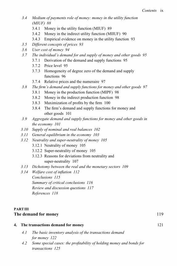
4. The transactions demand for money 121
4.1 The basic inventory analysis of the transactions demandfor money 122
4.2 Some special cases: the profitability of holding money and bonds fortransactions 125

x Contents
4.3 Demand for currency versus demand deposits 1274.4 Impact of economies of scale and income distribution 1284.5 Efficient funds management by firms 1294.6 The demand for money and the payment of interest on demand
deposits 1304.7 Demand deposits versus savings deposits 1314.8 Technical innovations and the demand for monetary assets 1324.9 Estimating money demand 133
Conclusions 135Summary of critical conclusions 136Review and discussion questions 136References 137
5. Portfolio selection and the speculative demand for money 138
5.1 Probabilities, means and variances 1405.2 Wealth maximization versus expected utility maximization 1425.3 Risk preference, indifference and aversion 144
5.3.1 Indifference loci for a risk averter 1455.4 The expected utility hypothesis of portfolio selection 1455.5 The efficient opportunity locus 147
5.5.1 Expected value and standard deviation of the portfolio 1475.5.2 Opportunity locus for a riskless asset and a risky asset 1485.5.3 Opportunity locus for risky assets 1485.5.4 Efficient opportunity locus 1515.5.5 Optimal choice 151
5.6 Tobin’s analysis of the demand for a riskless asset versusa risky one 154
5.7 Specific forms of the expected utility function 1585.7.1 EUH and measures of risk aversion 1585.7.2 Constant absolute risk aversion (CARA) 1595.7.3 Constant relative risk aversion (CRRA) 1625.7.4 Quadratic utility function 164
5.8 Volatility of the money demand function 1655.9 Is there a positive portfolio demand for money balances in
the modern economy? 165Conclusions 167Appendix 1 167Axioms and theorem of the expected utility hypothesis 167Appendix 2 169Opportunity locus for two risky assets 169Summary of critical conclusions 172Review and discussion questions 172References 174
Contents xi
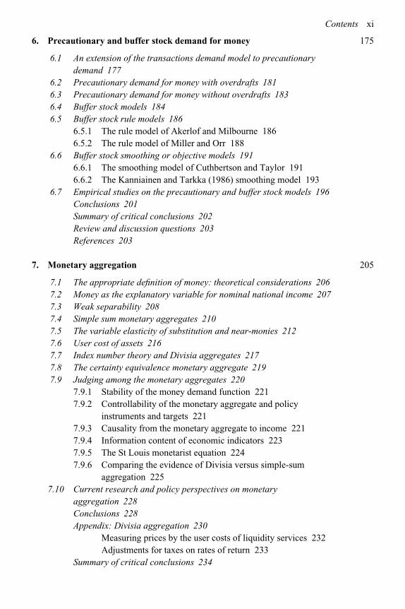
6. Precautionary and buffer stock demand for money 175
6.1 An extension of the transactions demand model to precautionarydemand 177
6.2 Precautionary demand for money with overdrafts 1816.3 Precautionary demand for money without overdrafts 1836.4 Buffer stock models 1846.5 Buffer stock rule models 186
6.5.1 The rule model of Akerlof and Milbourne 1866.5.2 The rule model of Miller and Orr 188
6.6 Buffer stock smoothing or objective models 1916.6.1 The smoothing model of Cuthbertson and Taylor 1916.6.2 The Kanniainen and Tarkka (1986) smoothing model 193
6.7 Empirical studies on the precautionary and buffer stock models 196Conclusions 201Summary of critical conclusions 202Review and discussion questions 203References 203
7. Monetary aggregation 205
7.1 The appropriate definition of money: theoretical considerations 2067.2 Money as the explanatory variable for nominal national income 2077.3 Weak separability 2087.4 Simple sum monetary aggregates 2107.5 The variable elasticity of substitution and near-monies 2127.6 User cost of assets 2167.7 Index number theory and Divisia aggregates 2177.8 The certainty equivalence monetary aggregate 2197.9 Judging among the monetary aggregates 220
7.9.1 Stability of the money demand function 2217.9.2 Controllability of the monetary aggregate and policy
instruments and targets 2217.9.3 Causality from the monetary aggregate to income 2217.9.4 Information content of economic indicators 2237.9.5 The St Louis monetarist equation 2247.9.6 Comparing the evidence of Divisia versus simple-sum
aggregation 2257.10 Current research and policy perspectives on monetary
aggregation 228Conclusions 228Appendix: Divisia aggregation 230
Measuring prices by the user costs of liquidity services 232Adjustments for taxes on rates of return 233
Summary of critical conclusions 234

xii Contents
Review and discussion questions 234References 235
8. The demand function for money 237
8.1 Basic functional forms of the closed-economy money demandfunction 2388.1.1 Scale variable in the money demand function 240
8.2 Rational expectations 2418.2.1 Theory of rational expectations 2418.2.2 Information requirements of rational expectations:
an aside 2438.2.3 Using the REH and the Lucas supply rule for predicting
expected income 2458.2.4 Using the REH and a Keynesian supply function for predicting
expected income 2478.2.5 Rational expectations – problems and approximations 248
8.3 Adaptive expectations for the derivation of permanent income andestimation of money demand 249
8.4 Regressive and extrapolative expectations 2518.5 Lags in adjustment and the costs of changing money balances 2528.6 Money demand with the first-order PAM 2548.7 Money demand with the first-order PAM and adaptive expectations of
permanent income 2558.8 Autoregressive distributed lag model: an introduction 2568.9 Demand for money in the open economy 257
8.9.1 Theories of currency substitution 2588.9.2 Estimation procedures and problems 2618.9.3 The special relation between M and M ∗ in the
medium-of-payments function 2648.9.4 Other studies on CS 266Conclusions 267Summary of critical conclusions 268Review and discussion questions 268References 269
9. The demand function for money: Estimation problems, techniques andfindings 270
9.1 Historical review of the estimation of money demand 2719.2 Common problems in estimation: an introduction 275
9.2.1 Single equation versus simultaneous equations estimation 2769.2.2 Estimation restrictions on the portfolio demand functions for
money and bonds 2769.2.3 The potential volatility of the money demand function 277

Contents xiii
9.2.4 Multicollinearity 2789.2.5 Serial correlation and cointegration 278
9.3 The relationship between economic theory and cointegration analysis:a primer 2799.3.1 Economic theory: equilibrium and the adjustment to
equilibrium 2799.4 Stationarity of variables: an introduction 280
9.4.1 Order of integration 2829.4.2 Testing for non-stationarity 283
9.5 Cointegration and error correction: an introduction 2849.5.1 Cointegration techniques 286
9.6 Cointegration, ECM and macroeconomic theory 2889.7 Application of the cointegration–ECM technique to money demand
estimation 2889.8 Some cointegration studies of the money-demand function 2899.9 Causality 2929.10 An illustration: money demand elasicities in a period of
innovation 2929.11 Innovations and the search for a stable money-demand function 293
Conclusions 294Summary of critical conclusions 296Appendix 297
The ARDL model and its cointegration and ECM forms 297Review and discussion questions 298References 300
PARTIV
Monetary policy and central banking 303
10. Money supply, interest rates and the operating targets of monetarypolicy: Money supply and interest rates 305
10.1 Goals, targets and instruments of monetary policy 30610.2 Relationship between goals, targets and instruments, and difficulties
in the pursuit of monetary policy 30810.3 Targets of monetary policy 30910.4 Monetary aggregates versus interest rates as operating targets 309
10.4.1 Diagrammatic analysis of the choice of the operating target ofmonetary policy 310
10.4.2 Analysis of operating targets under a supply shock 31310.5 The price level and inflation rate as targets 31610.6 Determination of the money supply 319
10.6.1 Demand for currency by the public 31910.6.2 Commercial banks: the demand for reserves 322
xiv Contents
10.7 Mechanical theories of the money supply: money supplyidentities 325
10.8 Behavioral theories of the money supply 32710.9 Cointegration and error-correction models of the money
supply 33110.10 Monetary base and interest rates as alternative policy
instruments 331Conclusions 333Summary of critical conclusions 334Review and discussion questions 334References 336
11. The central bank: Goals, targets and instruments 338
11.1 Historic goals of central banks 33911.2 Evolution of the goals of central banks 34211.3 Instruments of monetary policy 345
11.3.1 Open market operations 34511.3.2 Reserve requirements 34611.3.3 Discount/bank rate 34811.3.4 Moral suasion 35111.3.5 Selective controls 35111.3.6 Borrowed reserves 35211.3.7 Regulation and reform of commercial banks 352
11.4 Efficiency and competition in the financial sector: competitive supplyof money 35311.4.1 Arguments for the competitive supplies of private monies 35311.4.2 Arguments for the regulation of the money supply 35411.4.3 Regulation of banks in the interests of monetary policy 354
11.5 Administered interest rates and economic performance 35611.6 Monetary conditions index 35711.7 Inflation targeting and the Taylor rule 35811.8 Currency boards 359
Conclusions 360Summary of critical conclusions 361Review and discussion questions 361References 362
12. The central bank: Independence, time consistency and credibility 364
12.1 Choosing among multiple goals 36512.2 Conflicts among policy makers: theoretical analysis 36812.3 Independence of the central bank 37012.4 Time consistency of policies 373
12.4.1 Time-consistent policy path 37412.4.2 Reoptimization policy path 376
Contents xv
12.4.3 Limitations on the superiority of time-consistent policies overreoptimization policies 377
12.4.4 Inflationary bias of myopic optimization versus intertemporaloptimization 381
12.4.5 Time consistency debate: modern classical versus Keynesianapproaches 381
12.4.6 Objective functions for the central bank and the economy’sconstraints 382
12.5 Commitment and credibility of monetary policy 38712.5.1 Expectations, credibility and the loss from discretion versus
commitment 38712.5.2 Credibility and the costs of disinflation under the EAPC 39112.5.3 Gains from credibility with a target output rate greater
than yf 39312.5.4 Analyses of credibility and commitment under supply shocks
and rational expectations 39512.6 Does the central bank possess information superiority? 39812.7 Empirical relevance of the preceding analyses 398
Conclusions 399Appendix 401
Myopic optimal monetary policy without commitment in anew Keynesian framework 401Intertemporal optimization with commitment in a newKeynesian framework 403
Summary of critical conclusions 403Review and discussion questions 404References 405
PARTV
Monetary policy and the macroeconomy 407
13. The determination of aggregate demand 409
13.1 Boundaries of the short-run macroeconomic models 41013.1.1 Definitions of the short-run and long-run in
macroeconomics 41013.2 The foreign exchange sector of the open economy and the
determination of the exchange rate under floating exchange rates 41113.3 The commodity sector 413
13.3.1 Behavioral functions of the commodity market 41513.4 The monetary sector: determining the appropriate operating target of
monetary policy 41813.5 Derivation of the LM equation 419
13.5.1 The link between the IS and LM equations: the Fisher equationon interest rates 421

xvi Contents
13.6 Aggregate demand for commodities in the IS–LM model 42113.6.1 Keynesian–neoclassical synthesis on aggregate demand in the
IS–LM model 42413.7 Ricardian equivalence and the impact of fiscal policy on aggregate
demand in the IS–LM model 42413.8 IS–LM model under a Taylor-type rule for the money supply 42913.9 Short-run macro model under an interest rate operating
target 42913.9.1 Determination of aggregate demand under simple interest rate
targeting 43413.9.2 Aggregate demand under the Taylor rule 43513.9.3 Aggregate demand under the simple interest rate target and
Ricardian equivalence 43613.9.4 The potential for disequilibrium in the financial markets under
an interest rate target 43613.10 Does interest rate targeting make the money supply
redundant? 43913.11 Weaknesses of the IS–LM and IS–IRT analyses of aggregate
demand 44013.12 Optimal choice of the operating target of monetary policy 441
Conclusions 444Appendix 444
The propositions of Ricardian equivalence and the evolution ofthe public debt 444
Summary of critical conclusions 446Review and discussion questions 446References 449
14. The classical paradigm in macroeconomics 451
14.1 Definitions of the short run and the long run 45314.2 Long-run supply side of the neoclassical model 45414.3 General equilibrium: aggregate demand and supply analysis 45814.4 Iterative structure of the neoclassical model 461
14.4.1 The rate of unemployment and the natural rate ofunemployment 463
14.4.2 IS–LM version of the neoclassical model in a diagrammaticform 465
14.5 Fundamental assumptions of the Walrasian equilibrium analysis 46714.6 Disequilibrium in the neoclassical model and the non-neutrality
of money 46814.6.1 Pigou and real balance effects 46814.6.2 Causes of deviations from long-run equilibrium 470
14.7 The relationship between the money supply and the price level: theheritage of ideas 471

Contents xvii
14.8 The classical and neoclassical tradition, economic liberalism andlaissez faire 47214.8.1 Some major misconceptions about traditional classical and
neoclassical approaches 47414.9 Uncertainty and expectations in the classical paradigm 47514.10 Expectations and the labor market: the expectations-augmented
Phillips curve 47614.10.1 Output and employment in the context of nominal wage
contracts 47614.10.2 The Friedman supply rule 48114.10.3 Expectations-augmented employment and output
functions 48214.10.4 The short-run equilibrium unemployment rate and
Friedman’s expectations-augmented Phillips curve 48314.11 Price expectations and commodity markets: the Lucas supply
function 48514.12 The Lucas model with supply and demand functions 48814.13 Defining and demarcating the models of the classical paradigm 49214.14 Real business cycle theory and monetary policy 49514.15 Milton Friedman and monetarism 49714.16 Empirical evidence 501
Conclusions 503Summary of critical conclusions 504Review and discussion questions 505References 507
15. The Keynesian paradigm 510
15.1 Keynesian model I: models without efficient labor markets 51415.1.1 Keynesian deficient-demand model: quantity-constrained
analysis 51715.2 Keynesian model II: Phillips curve analysis 52215.3 Components of neoKeynesian economics 525
15.3.1 Efficiency wage theory 52515.3.2 Costs of adjusting employment: implicit contracts and labor
hoarding 52715.3.3 Price stickiness 528
15.4 New Keynesian (NK) macroeconomics 53215.4.1 NK commodity market analysis 53315.4.2 NK price adjustment analysis 53415.4.3 Other reasons for sticky prices, output and employment 53715.4.4 Interest rate determination 53915.4.5 Variations of the overall NK model 54315.4.6 Money supply in the NK model 54415.4.7 NK business cycle theory 548

xviii Contents
15.5 Reduced-form equations for output and employment in the Keynesianand neoclassical approaches 549
15.6 Empirical validity of the new Keynesian ideas 551Conclusions 552Summary of critical conclusions 556Review and discussion questions 557References 561
16. Money, bonds and credit in macro modeling 563
16.1 Distinctiveness of credit from bonds 57016.1.1 Information imperfections in financial markets 570
16.2 Supply of commodities and the demand for credit 57516.3 Aggregate demand analysis incorporating credit as a
distinctive asset 57716.3.1 Commodity market analysis 57716.3.2 Money market analysis 57716.3.3 Credit market analysis 57916.3.4 Determination of aggregate demand 581
16.4 Determination of output 58216.5 Impact of monetary and fiscal policies 58316.6 Instability in the money and credit markets and monetary
policy 58516.7 Credit channel when the bond interest rate is the exogenous monetary
policy instrument 58716.8 The informal financial sector and financial underdevelopment 58816.9 Bank runs and credit crises 58816.10 Empirical findings 589
Conclusions 591Appendix A 592
Demand for working capital for a given production level ina simple stylized model 592
Appendix B 593Indirect production function including working capital 593
Summary of critical conclusions 595Review and discussion questions 595References 596
17. Macro models and perspectives on the neutrality of money 599
17.1 The Lucas–Sargent–Wallace (LSW) analysis of the classicalparadigm 600
17.2 A compact (Model II) form of the LSW model 60517.3 The Lucas critique of estimated equations as a policy tool 606

Contents xix
17.4 Testing the effectiveness of monetary policy: estimates based on theLucas and Friedman supply models 60717.4.1 A procedure for segmenting the money supply changes into
their anticipated and unanticipated components 60817.4.2 Separating neutrality from rational expectations: Mishkin’s
test of the Lucas model 61017.5 Distinguishing between the impact of positive and negative money
supply shocks 61117.6 LSW model with a Taylor rule for the interest rate 61217.7 Testing the effectiveness of monetary policy: estimates from
Keynesian models 61517.7.1 Using the LSW model with a Keynesian supply
equation 61517.7.2 Gali’s version of the Keynesian model with an exogenous
money supply 61617.8 A compact form of the closed-economy new Keynesian model 618
17.8.1 Empirical findings on the new Keynesian model 61917.8.2 Ball’s Keynesian small open-economy model with a
Taylor rule 62117.9 Results of other testing procedures 62217.10 Summing up the empirical evidence on monetary neutrality and
rational expectations 62217.11 Getting away from dogma 623
17.11.1 The output equation revisited 62417.11.2 The Phillips curve revisited 625
17.12 Hysteresis in long-run output and employment functions 626Conclusions 626Summary of critical conclusions 630Review and discussion questions 630References 634
18. Walras’s law and the interaction among markets 636
18.1 Walras’s law 63718.1.1 Walras’s law in a macroeconomic model with four
goods 64018.1.2 The implication of Walras’s law for a specific market 641
18.2 Walras’s law and selection among the markets for a model 64118.3 Walras’s law and the assumption of continuous full employment 64318.4 Say’s law 64318.5 Walras’s law, Say’s law and the dichotomy between the real and
monetary sectors 64618.6 The wealth effect 64618.7 The real balance effect 647

xx Contents
18.8 Is Walras’s law really a law? When might it not hold? 64818.8.1 Intuition: violation of Walras’s law in recessions 64818.8.2 Walras’s law under excess demand for commodities 65118.8.3 Correction of Walras’s law 651
18.9 Notional demand and supply functions in the classical paradigm 65218.10 Re-evaluating Walras’s law 652
18.10.1 Fundamental causes of the failure of Walras’s law 65218.10.2 Irrationality of the behavioral assumptions behind Walras’s
law 65318.11 Reformulating Walras’s law: the Clower and Drèze effective demand
and supply functions 65318.11.1 Clower effective functions 65318.11.2 Modification of Walras’s law for Clower effective
functions 65418.11.3 Drèze effective functions and Walras’s law 654
18.12 Implications of the invalidity of Walras’s law for monetary policy 655Conclusions 655Summary of critical conclusions 656Review and discussion questions 656References 658
PARTVI
The rates of interest in the economy 659
19. The macroeconomic theory of the rate of interest 661
19.1 Nominal and real rates of interest 66219.2 Application of Walras’s law in the IS–LM models: the excess demand
for bonds 66319.2.1 Walras’s law 663
19.3 Derivation of the general excess demand function for bonds 66519.4 Intuition: the demand and supply of bonds and interest rate
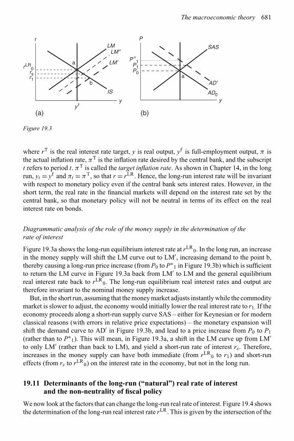
determination 66719.5 Intuition: dynamic determination of the interest rate 66919.6 The bond market in the IS LM diagram 670
19.6.1 Diagrammatic analysis of dynamic changes in the rateof interest 673
19.7 Classical heritage: the loanable funds theory of the rateof interest 67319.7.1 Loanable funds theory in the modern classical approach 67519.7.2 David Hume on the rate of interest 676
19.8 Keynesian heritage: the liquidity preference theory of theinterest rate 678
19.9 Comparing the liquidity preference and the loanable fundstheories of interest 679

Contents xxi
19.10 Neutrality versus non-neutrality of the money supply for the real rateof interest 680
19.11 Determinants of the long-run (“natural”) real rate of interest and thenon-neutrality of fiscal policy 681
19.12 Empirical evidence: testing the Fisher equation 68319.13 Testing the liquidity preference and loanable funds theories 683
Conclusions 686Summary of critical conclusions 687Review and discussion questions 687References 689
20. The structure of interest rates 690
20.1 Some of the concepts of the rate of interest 69120.2 Term structure of interest rates 692
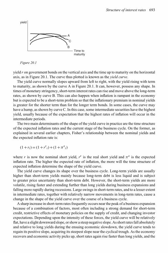
20.2.1 Yield curve 69220.2.2 Expectations hypothesis 69420.2.3 Liquidity preference version of the expectations
hypothesis 69720.2.4 Segmented markets hypothesis 69820.2.5 Preferred habitat hypothesis 69820.2.6 Implications of the term structure hypotheses for monetary
policy 69920.3 Financial asset prices 69920.4 Empirical estimation and tests 701
20.4.1 Reduced-form approaches to the estimation of the termstructure of yields 701
20.5 Tests of the expectations hypothesis with a constant premium andrational expectations 70220.5.1 Slope sensitivity test 70320.5.2 Efficient and rational information usage test 704
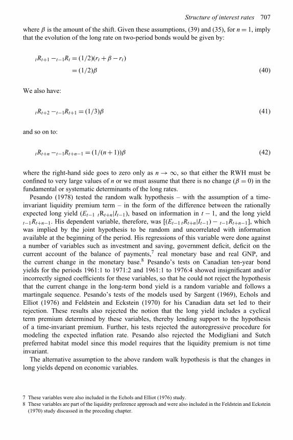
20.6 Random walk hypothesis of the long rates of interest 70520.7 Information content of the term structure for the expected rates of
inflation 708Conclusions 710Summary of critical conclusions 711Review and discussion questions 711References 712
PARTVII
Overlapping generations models of money 715
21. The benchmark overlapping generations model of fiat money 717
21.1 Stylized empirical facts about money in the modern economy 71821.2 Common themes about money in OLG models 719

xxii Contents
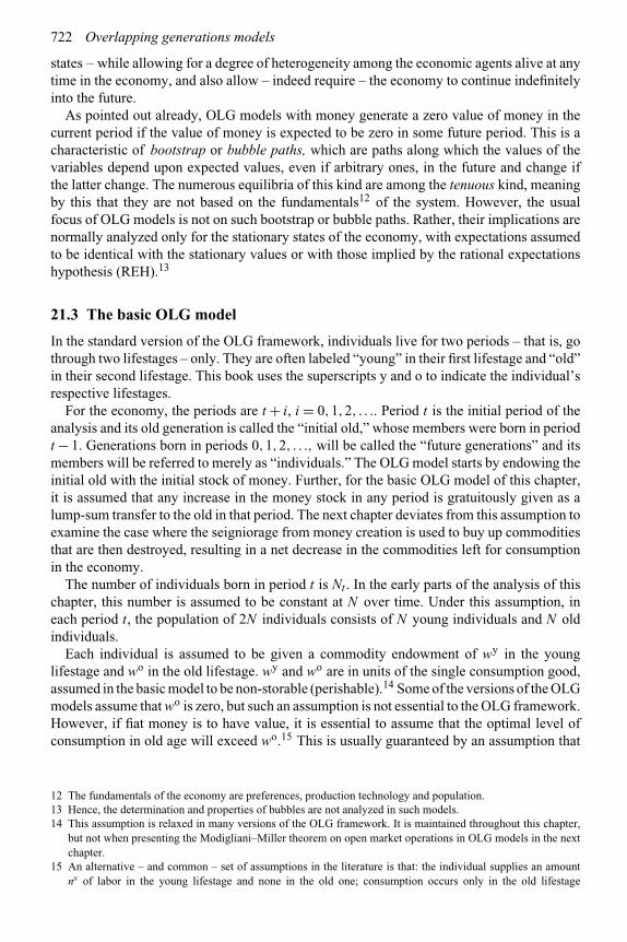
21.3 The basic OLG model 72221.3.1 Microeconomic behavior: the individual’s saving and
money demand 72321.3.2 Macroeconomic analysis: the price level and the value
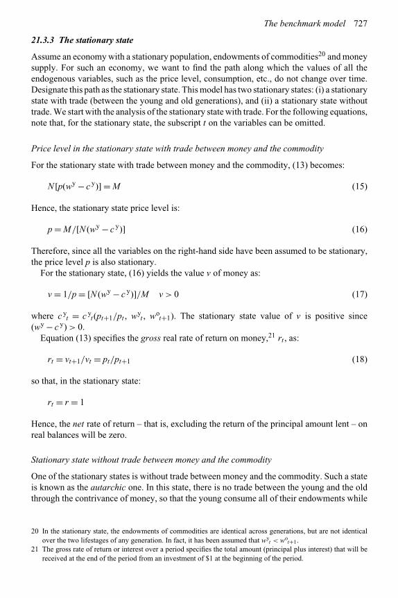
of money 72521.3.3 The stationary state 72721.3.4 Indeterminacy of the price level and of the value of
fiat money 72821.3.5 Competitive issue of money 729
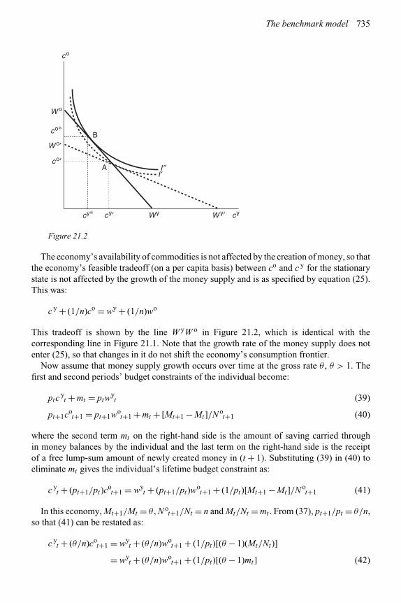
21.4 The basic OLG model with a growing population 72921.5 Welfare in the basic OLG model 73121.6 The basic OLG model with money supply growth and a growing
population 73321.7 Inefficiency of monetary expansion in the money transfer case 73421.8 Inefficiency of price stability with monetary expansion and population
growth 73821.9 Money demand in the OLG model with a positive rate of time
preference 73821.10 Several fiat monies 74021.11 Sunspots, bubbles and market fundamentals in OLG analysis 741
Conclusions 742Summary of critical conclusions 743Review and discussion questions 743References 744
22. The OLG model: Seigniorage, bonds and the neutrality of fiat money 746
22.1 Seigniorage from fiat money and its uses 74722.1.1 Value of money under seigniorage with destruction of
government-purchased commodities 74822.1.2 Inefficiency of monetary expansion with seigniorage as a
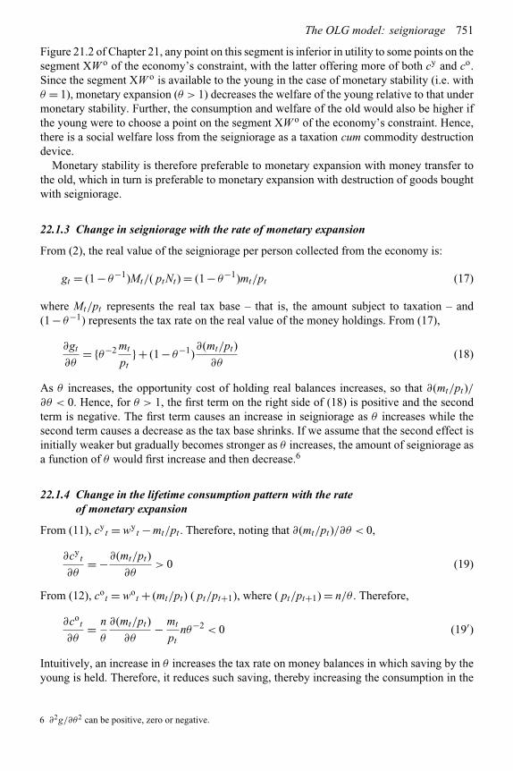
taxation device 74922.1.3 Change in seigniorage with the rate of monetary expansion 75122.1.4 Change in the lifetime consumption pattern with the rate of
monetary expansion 75122.1.5 Seigniorage from monetary expansion versus lump-sum
taxation 75222.1.6 Seigniorage as a revenue collection device 752
22.2 Fiat money and bonds in the OLG framework 75322.3 Wallace–Modigliani–Miller (W–M–M) theorem on open market
operations 75522.3.1 W–M–M theorem on open market operations with
commodity storage 75522.3.2 W–M–M theorem on open market operations in the
money–bonds OLG model 758

Contents xxiii
22.4 Getting beyond the simplistic OLG analysis of money 76022.4.1 Model I: an OLG model with money, capital and
production 76022.4.2 Model II: the preceding OLG model with a linear
production function 76422.5 Model III: the Lucas OLG model with non-neutrality of money 76422.6 Do the OLG models explain the major facets of a monetary
economy? 767Conclusions 770Summary of critical conclusions 771Review and discussion questions 771References 772
23. The OLG model of money: Making it more realistic 773
23.1 A T-period cash-in-advance money–bonds model 77523.1.1 Cash-in-advance models with money and one-period
bonds 77723.1.2 Analysis of the extended multi-period OLG cash-in-advance
money–bonds model 77723.1.3 W–M–M theorem in the extended OLG cash-in-advance
money–bonds model 78123.2 An extended OLG model with payments time for purchases and the
indirect MIUF 78423.2.1 OLG model extended to incorporate money indirectly in the
utility function (MIIUF) 78523.3 An extended OLG model for firms with money indirectly in the
production function (MIIPF) 79023.3.1 Rationale for putting real balances in the production
function 79023.3.2 Profit maximization and the demand for money by the firm 79223.3.3 Intuitive empirical evidence 793
23.4 Basic OLG model with MIIUF and MIIPF 795Conclusions 796Summary of critical conclusions 797Review and discussion questions 798References 799
PARTVIII
Money and financial institutions in growth theory 801
24. Monetary growth theory 803
24.1 Commodity money, real balances and growth theory 80624.2 Fiat balances in disposable income and growth 808
xxiv Contents
24.3 Real fiat balances in the static production function 81124.4 Reformulation of the neoclassical model with money in the static
production and utility functions 81224.5 Why and how does money contribute to per capita output and its
growth rate? 81524.6 How does the use of money change the labor supplied for
production? 81624.7 Distinction between inside and outside money 81724.8 Financial intermediation (FI) in the growth and development
processes 81724.9 The financial system 81824.10 Empirical evidence on the importance of money and the financial
sector to growth 82224.11 A simplified growth model of endogenous technical change involving
the financial sector 82724.12 Investment, financial intermediation and economic development 828
Conclusions 829Summary of critical conclusions 831Review and discussion questions 831References 832
Index 835

Preface
This book represents a comprehensive presentation of monetary economics. It integratesthe presentation of monetary theory with its heritage, its empirical formulations and theireconometric tests. While its main focus is on monetary theory and its empirical testsrather than on the institutional monetary and financial structure of the economy, the latteris brought in wherever needed for elucidating a theory or showing the limitations to itsapplicability. The illustrations for this purpose, as well as the empirical studies cited, aretaken from the United States, Canada and the United Kingdom. The book also elucidates thesignificant differences between the financially developed economies and the less developedand developing ones.
In addition, the presentation also provides an introduction to the main historical patternsof monetary thought and the diversity of ideas in monetary economics, especially on theeffectiveness of monetary policy and the contending schools in monetary theory and policy.
Our presentation of the theoretical aspects of monetary economics is tempered by thegoals of empirical relevance and validity, and intuitive understanding. The derivation of thetheoretical implications is followed by a discussion of their simplifications and modificationsmade in the process of econometric testing, as well as a presentation of the empirical findings.
Part I of the book consists of the introduction to monetary economics and its heritage. Thelatter is not meant to be exhaustive but is intended to illustrate the evolution of monetarythought and to provide the reader with a flavor of the earlier literature on this subject.
Part II places monetary microeconomics in the context of the Walrasian general equilibriummodel. To derive the demand for money, it uses the approaches of money in the utility functionand in the production function. It then derives the Walrasian results on the neutrality of moneyand the dichotomy between the monetary and real sectors of the economy.
Part III focuses on the demand for money. Besides the usual treatment of transactionsand speculative demands, this part also presents models of the precautionary and bufferstock demand for money. The theoretical chapters on the components of money demandare followed by three chapters on its empirical aspects, including a separate chapter on thecriteria and tests underlying monetary aggregation.
Part IV deals with the supply of money and the role of the central bank in determining themoney supply and interest rates. It compares the desirability of monetary versus interest rate asoperating targets. This part also examines the important policy issues of the potential conflictsamong policy makers, central bank independence, time-consistent versus discretionarymonetary policies, and the credibility of monetary policy.
No presentation of monetary economics can be complete without adequate coverageof monetary policy and its impact on the macroeconomy. Proper treatment of this topicrequires knowledge of the underlying macroeconomic models and their implications for

xxvi Preface
monetary policy. Part V focuses on money and monetary policy in the macroeconomy.It covers the main macroeconomic models of both the classical and Keynesian paradigmsand their monetary implications. This coverage includes extensive analysis of the Taylor rulefor targeting inflation and the output gap, and new Keynesian economics.
The remaining parts of the book deal with special topics. Part VI deals with the theories ofthe rate of interest and of the term structure of interest rates. Part VII presents the overlappinggenerations models of fiat money and compares their implications and empirical validitywith those of the theories based on money in the utility function and money in the productionfunction. Part VIII addresses monetary growth theory, and assesses the contributions of boththe quantity of money and those of financial institutions to output growth. To do so, it coversthe neoclassical growth theory with money as well as endogenous growth theories withmoney.
Comparison with the first (2000) edition
This edition has extensive revisions and new material in all its chapters. However, since themajor ferment in monetary economics in the past decade has been in monetary policy andmonetary macroeconomics, most of the additional material is to be found in the chapters onthese issues. Chapter 12 has more extensive discussion of central bank independence, timeconsistency versus intertemporal re-optimization, and credibility. Chapter 13 is a new chapteron the determination of aggregate demand under the alternative operating targets of moneysupply and interest rates. Chapter 14, on the classical paradigm, now starts with a presentationof the stylized facts on the relationship between money, inflation and output, and includesmore detailed evaluation of the validity of the latest model, the modern classical one, in theclassical paradigm. Chapter 15, on the Keynesian paradigm, has considerably more materialon the Taylor rule, and on the new Keynesian model, as well as discussion of its validity.Chapter 16, on the role of credit markets in the macroeconomy, is entirely new. Chapter 17has been expanded to include compact models of the new Keynesian type, in addition to theLucas–Sargent–Wallace ones of the modern classical variety, as well as including greaterdiscussion of the validity of their implications. Chapter 21, on the overlapping generationsmodels, now starts with a presentation of the stylized facts on money, especially on its demandfunction, so as to more clearly assess the validity of the implications of such models.
Level and patterns of use of this book
This book is at the level of the advanced undergraduate and graduate courses in monetaryeconomics. It requires that the students have had at least one prior course in macroeconomicsand/or money and banking. It also assumes some knowledge of differential calculus andstatistics.
Given the large number of topics covered and the number of chapters, this book can beused over one semester on a quite selective basis or over two or three semesters on a fairlycomplete basis. It also offers considerable scope for the instructors to adapt the materialto their specific interests and to the levels of their courses by exercising selectivity in thechapters covered and the sequence of topics.
Some suggested patterns for one-term courses are:
1. Courses on monetary microeconomics (demand and supply of money) and policy:Chapters 1, 2, 3 (optional), 4, 5, 7–12.

Preface xxvii
2. Courses on monetary macroeconomics: Chapters 1, 2, 13–17 (possibly includingChapters 18–20).
3. Courses on monetary macroeconomics and central bank policies: Chapters 1, 2, 10–19.4. Courses on advanced topics in monetary economics: Chapters 3, 6, 16–24.
A first course along the lines of 1, 2 or 3 can be followed by a second course based on 4.McGill offers a tandem set of two one-term graduate courses covering money and banking
and monetary economics. The first term of these is also open to senior honours students. Thisbook came out of my lectures in these courses.
My students in the first one of the two courses almost invariably have shown a stronginterest in monetary policy and macroeconomics, and want their analyses to be covered at anearly stage, while I want also to cover the main material on the demand and supply of money.With two one-semester courses, I am able to allow the students a wide degree of latitude inselecting the pattern in which these topics are covered. The mutually satisfactory combinationin many years has often been to do in the first semester the introductory Chapters 1 and 2,monetary macroeconomics (Chapters 13 to 17), determination of interest rates (Chapters 19and 20) and possibly monetary growth theory (Chapter 24). The second term then coveredmoney demand and supply (Chapters 4 to 10) (excluding Chapter 6 on the precautionaryand buffer stock demands for money) and central banking (Chapters 10 to 12). However,we have in some years chosen to study the money demand and supply chapters before themonetary macroeconomics chapters. This arrangement left the more theoretical, advancedor special topics to be slotted along with the other material in one of the terms, or leftto another course. The special topics chapters are: 3 (general equilibrium with money), 6(precautionary and buffer stock models of money demand), 16 (credit markets), 17 (compactmacroeconomic models with money), 18 (Walras’s law and the interaction among markets),21 to 23 (overlapping generations models with money) and Chapter 24 (growth theory withmoney).

Acknowledgments
I am indebted to my students in monetary economics who suffered – and hopefully benefited –from several drafts of this manuscript. Many helped to improve it.
It is, as always, a pleasure to acknowledge the love and support of my wife, Sushma, andsons, Sunny and Rish, as well as of my other family members, Subash, Monica, Riley andAerin.
Professor Jagdish [email protected]

Part I
Introduction and heritage

1 Introduction
Monetary economics has both a microeconomics component and a macroeconomics one.The fundamental questions of monetary microeconomics concern the proper definition ofmoney and its demand and supply, and those of monetary macroeconomics concern theformulation of monetary policy and its impact on the economy.
The financial assets that can serve the medium of the payments role of money have changedover time, as has the elasticity of substitution among monetary assets, so that the properdefinition of money has also kept changing.
For short-run analysis, monetary economics is a central part of macroeconomics. The mainparadigms of macroeconomics are the classical and Keynesian ones. The former paradigmstudies the competitive economy at its full employment equilibrium, while the latter focuseson its deviations away from this equilibrium.
Key concepts introduced in this chapter
♦ Functions of money♦ M1, M2, and broader definitions of money♦ Financial intermediaries♦ Creation of money by banks♦ Classical paradigm for macroeconomics♦ Walrasian general equilibrium model♦ Neoclassical, traditional classical, modern classical and new classical models♦ Keynesian paradigm for macroeconomics♦ IS–LM analysis
Monetary economics is the economics of the money supply, prices and interest rates, andtheir repercussions on the economy. It focuses on the monetary and other financial markets,the determination of the interest rate, the extent to which these influence the behavior of theeconomic units and the implications of that influence in the macroeconomic context. It alsostudies the formulation of monetary policy, usually by the central bank or “the monetaryauthority,” with respect to the supply of money and manipulation of interest rates, in termsboth of what is actually done and what would be optimal.
In a monetary economy, virtually all exchanges of commodities among distinct economicagents are against money, rather than against labor, commodities or bonds, and virtually allloans are made in money and not in commodities, so that almost all market transactions in a

4 Introduction and heritage
modern monetary economy involve money.1 Therefore, few aspects of a monetary economyare totally divorced from the role of money and the efficiency of its provision and usage, andthe scope of monetary economics is a very wide one.
Monetary economics has both a microeconomics and a macroeconomics part. In addition,the formulation of monetary policy and central bank behavior – or that of “the monetaryauthority,” often a euphemism for the central banking system of the country2 – is an extremelyimportant topic which can be treated as a distinct one in its own right, or covered under themicroeconomics or macroeconomics presentation of monetary economics.
Microeconomics part of monetary economics
The microeconomics part of monetary economics focuses on the study of the demand andsupply of money and their equilibrium. No study of monetary economics can be evenminimally adequate without a study of the behavior of those financial institutions whosebehavior determines the money stock and its close substitutes, as well as determiningthe interest rates in the economy. The institutions supplying the main components of themoney stock are the central bank and the commercial banks. The commercial banks arethemselves part of the wider system of financial intermediaries, which determine the supplyof some of the components of money as well as the substitutes for money, also known asnear-monies.
The two major components of the microeconomics part of monetary economics arethe demand for money, covered in Chapters 4 to 9, and the supply of money, coveredin Chapter 10. The central bank and its formulation of monetary policy are covered inChapters 11 and 12.
Macroeconomics part of monetary economics: money in the macroeconomy
The macroeconomics part of monetary economics is closely integrated into the standard short-run macroeconomic theory. The reason for such closeness is that monetary phenomena arepervasive in their influence on virtually all the major macroeconomic variables in the short-run. Among variables influenced by the shifts in the supply and demand for money are nationaloutput and employment, the rate of unemployment, exports and imports, exchange rates andthe balance of payments. And among the most important questions in macroeconomic analysisare whether – to what extent and how – the changes in the money supply, prices and inflation,and interest rates affect the above variables, especially national output and employment. Thispart of monetary economics is presented in Chapters 13 to 20.
A departure from the traditional treatment of money in economic analysis is provided by theoverlapping generations models of money. These have different implications for monetarypolicy and its impact on the economy than the standard short-run macroeconomic models.
1 Even an economy that starts out without money soon discovers its usefulness and creates it in some form or other.The classic article by Radford (1945) provides an illustration of the evolution of money from a prisoner-of-warcamp in Germany during the Second World War.
2 In the United States and Canada, the control of monetary policy rests solely with the central bank, so that the centralbank alone constitutes the “monetary authority”. In the United Kingdom, control over the goals of monetary policyrests with the government while its implementation rests with the Bank of England (the central bank), so thatthe “monetary authority” in the UK is composed of the government in the exercise of its powers over monetarypolicy and the central bank.

Introduction 5
While most textbooks on monetary economics exclude the overlapping generations models ofmoney, they are an important new development in monetary economics. They are presentedin Chapters 21 to 23.
The long-run analysis of monetary economics is less extensive and, while macroeconomicgrowth theory is sometimes extended to include money, the resulting monetary growth theoryis only a small element of monetary economics. Monetary growth theory is covered inChapter 24.
There are different approaches to the macroeconomics of monetary policy. These includethe models of the classical paradigm (which encompass the Walrasian model, the classicaland neoclassical models) and those of the Keynes’s paradigm (which encompass Keynes’sideas, the Keynesian models and the new Keynesian models). We elucidate their differencesat an introductory level towards the end of this chapter. Their detailed exposition is given inChapters 13 to 17.
1.1 What is money and what does it do?
1.1.1 Functions of money
Money is not itself the name of a particular asset. Since the assets which function as money tendto change over time in any given country and among countries, it is best defined independentlyof the particular assets that may exist in the economy at any one time. At a theoretical level,money is defined in terms of the functions that it performs. The traditional specification ofthese functions is:
1 Medium of exchange/payments. This function was traditionally called the medium ofexchange. In a modern context, in which transactions can be conducted with credit cards,it is better to refer to it as the medium of (final) payments.
2 Store of value, sometimes specified as a temporary store of value or temporary abode ofpurchasing power.
3 Standard of deferred payments.4 Unit of account.
Of these functions, the medium of payments is the absolutely essential function of money.Any asset that does not directly perform this function – or cannot indirectly perform it througha quick and costless transfer into a medium of payments – cannot be designated as money.A developed economy usually has many assets which can perform such a role, though somedo so better than others. The particular assets that perform this role vary over time, withcurrency being the only or main medium of payments early in the evolution of monetaryeconomies. It is complemented by demand deposits with the arrival of the banking systemand then by an increasing array of financial assets as other financial intermediaries becomeestablished.
1.1.2 Definitions of money
Historically, the definitions of money have measured the quantity of money in the economyas the sum of those items that serve as media of payments in the economy. However, at anytime in a developed monetary economy, there may be other items that do not directly serve asa medium of payments but are readily convertible into the medium of payments at little cost

6 Introduction and heritage
and trouble and can simultaneously be a store of value. Such items are close substitutes forthe medium of payments itself. Consequently, there is a considerable measure of controversyand disagreement about whether to confine the definition of money to the narrow role of themedium of payments or to include in this definition those items that are close substitutes forthe medium of payments.3
A theoretically oriented answer to this question would aim at a pure definition: money isthat good which serves directly as a medium of payments. In financially developed economies,this role is performed by currency held by the public and the public’s checkable deposits infinancial institutions, mainly commercial banks, with their sum being assigned the symbolM1 and called the narrow definition of money. The checkable or demand deposits in questionare ones against which withdrawals can be made by check or debit cards. Close substitutesto money thus defined as the medium of payments are referred to as near-monies.
An empirical answer to the definition of the money stock is much more eclectic than itstheoretical counterpart. It could define money narrowly or broadly, depending upon whatsubstitutes to the medium of payments are included or excluded. The broad definition thathas won the widest acceptance among economists is known as (Milton) Friedman’s definitionof money or as the broad definition of money. It defines money as the sum of currency in thehands of the public plus all of the public’s deposits in commercial banks. The latter includedemand deposits as well as savings deposits in commercial banks. Friedman’s definition ofmoney is often symbolized as M2, with variants of M2 designated as M2+, M2++, or asM2A, M2B, etc. However, there are now in usage many still broader definitions, usuallydesignated as M3, M4, etc.
A still broader definition of money than Friedman’s definition is M2 plus deposits innear-banks – i.e. those financial institutions in which the deposits perform almost the samerole for depositors as similar deposits in commercial banks. Examples of such institutionsare savings and loan associations and mutual savings banks in the United States; creditunions, trust companies and mortgage loan companies in Canada; and building societies inthe United Kingdom. The incorporation of such deposits into the measurement of money isdesignated by the symbols M3, M4, etc., by M2A, M2B, or by M2+, M2++, etc. However,the definitions of these symbols have not become standardized and remain country specific.Their specification, and the basis for choosing among them, are given briefly later in thischapter and discussed more fully in Chapter 7.
1.2 Money supply and money stock
Money is a good, which, just like other goods, is demanded and supplied by economicagents in the economy. There are a number of determinants of the demand and supply ofmoney. The most important of the determinants of money demand are national income,the price level and interest rates, while that of money supply is the behavior of the centralbank of the country which is given the power to control the money supply and bring aboutchanges in it.
The equilibrium amount in the market for money specifies the money stock, as opposedto the money supply, which is a behavioral function specifying the amount that would besupplied at various interest rates and income levels. The equilibrium amount of money is theamount for which money demand and money supply are equal.
3 Goodhart (1984).

Introduction 7
The money supply and the money stock are identical in the case where the money supplyis exogenously determined, usually by the policies of the central bank. In such a case, it isindependent of the interest rate and other economic variables, though it may influence them.Much of the monetary and macroeconomic reasoning of a theoretical nature assumes thiscase, so that the terms “money stock” and “money supply” are used synonymously. One has tojudge from the context whether the two concepts are being used as distinct or as identical ones.
The control of the money supply rests with the monetary authorities. Their policy withrespect to changes in the money supply is known as monetary policy.
1.3 Nominal versus the real value of money
The nominal value of money is in terms of money itself as the measuring unit. The real valueof money is in terms of its purchasing power over commodities. Thus, the nominal value of a$1 note is 1 – and that of a $20 note is 20. The real value of money is the amount of goods andservices one unit of money can buy and is the reciprocal of the price level of commoditiestraded in the economy. It equals 1/P where P is the average price level in the economy. Thereal value of money is what we usually mean when we use the term “the value of money.”
1.4 Money and bond markets in monetary macroeconomics
The “money market” in monetary and macroeconomics is defined as the market in which thedemand and supply of money interact, with equilibrium representing its clearance. However,the common English-language usage of this term refers to the market for short-term bonds,especially that of Treasury bills. To illustrate this common usage, this definition is embodiedin the term “money market mutual funds,” which are mutual funds with holdings of short-term bonds. It is important to note that our usage of the term “the money market” in this bookwill follow that of macroeconomics. To reiterate, we will mean by it the market for money,not the market for short-term bonds.
The usual custom in monetary and macroeconomics is to define “bonds” to cover all non-monetary financial assets, including loans and shares, so that the words “bonds,” “credit”and “loans” are treated as synonymous. Given this usage, the “bond/credit/loan market” isdefined as the market for all non-monetary financial assets. We will maintain this usage inthis book except in Chapter 16, which creates a distinction between marketable bonds andnon-marketable loans.
1.5 A brief history of the definition of money
The multiplicity of the functions performed by money does not aid in the task ofunambiguously identifying particular assets with money and often poses severe problemsfor such identification, since different assets perform these functions to varying degrees.Problems with an empirical measure of money are not new, nor have they necessarily takentheir most acute form only recently.
Early stages in the evolution from a barter economy to a monetary economy usually haveone or more commodity monies. One form of these is currency in the form of coins made ofa precious metal, with an exchange value which is, at least roughly, equal to the value of themetal in the coin. These coins were usually minted with the monarch’s authority and weredeclared to be “legal tender,” which obligated the seller or creditor to accept them in payment.
Legal tender was in certain circumstances supplemented as a means of payment bythe promissory notes of trustworthy persons or institutions and, in the eighteenth and

8 Introduction and heritage
nineteenth centuries, by bills of exchange4 in Britain. However, they never became agenerally accepted medium of payment. The emergence of private commercial banks5 afterthe eighteenth century in Britain led to (private) note issues6 by them and eventually alsoto orders of withdrawal – i.e. check – drawn upon these banks by those holding demanddeposits with them. However, while the keeping of demand deposits with banks had becomecommon among firms and richer individuals by the beginning of the twentieth century, thepopularity of such deposits among ordinary persons came only in the twentieth century.With this popularity, demand deposits became a component of the medium of payments inthe economy, with their amount eventually becoming larger than that of currency.
In Britain, in the mid-nineteenth century, economists and bankers faced the problem ofwhether to treat the demand liabilities of commercial banks, in addition to currency, as moneyor not. Commercial banking was still in its infancy and was confined to richer individuals andlarger firms. While checks functioned as a medium for payments among these groups, mostof the population did not use them. In such a context, there was considerable controversyon the proper definition of money and the appropriate monetary policies and regulationsin mid-nineteenth century England. These disputes revolved around the emergence of bankdemand deposits as a substitute, though yet quite imperfect, for currency and whether ornot the former were a part of the money supply. Further evolution of demand deposits andof banks in the late nineteenth century and the first half of the twentieth century in Britain,Canada and the USA led to the relative security and common usage of demand deposits andestablished their close substitutability for currency. Consequently, the accepted definition ofmoney by the second quarter of the twentieth century had become currency in the hands ofthe public plus demand deposits in commercial banks. During this period, saving depositswere not checkable and the banks holding them could insist on due notice being given priorto withdrawal personally by the depositor, so that they were not as liquid as demand depositsand were not taken to be money, defined as the medium of payments. Consequently, untilthe second half of the twentieth century, the standard definition of money was the narrowdefinition of money, denoted as M1.
Until the mid-twentieth century, demand deposits in most countries did not pay interestbut savings deposits in commercial banks did do so, though subject to legal or customaryceilings on their interest rates. During the 1950s, changes in banking practices caused thesesavings deposits to increasingly become closer substitutes for demand deposits so that themajor dispute of the 1950s on the definition of money was whether savings deposits shouldor should not be included in the definition of money. However, by the early 1960s, mosteconomists had come to measure the supply of money by M2 – that is, as M1 plus savings
4 A bill of exchange is a promissory note issued by a buyer of commodities and promises to pay a specified sum ofmoney to the seller on a specific future date. As such, they arise in the course of trade where the buyer does not payfor the goods immediately but is extended credit for the value of the goods for a short period, often three months.This delay allows the buyer time to sell the goods, so that the proceeds can be used to pay the original seller.In the nineteenth century, bills of exchange issued by reputable firms could be traded in the financial markets ordiscounted (i.e. sold at a discount to cover the interest) with banks. Some of them passed from hand to hand (i.e.were sold several times).
5 Many of the bankers were originally goldsmiths who maintained safety vaults and whose customers would depositgold coins with them for security reasons. When a depositor needed to make a payment to someone, he couldwrite a note/letter authorizing the recipient to withdraw a certain amount from the deposits of the payer with thegoldsmith.
6 Private note issues were phased out in most Western countries by the early twentieth century and replaced by amonopoly granted to the central bank of the power to issue notes.

Introduction 9
deposits in commercial banks – which does not include any types of deposits in other financialinstitutions. This mode of defining M2 is known as the Friedman definition (measure) ofmoney, since Milton Friedman had been one of its main proponents in the 1950s and 1960s.
In the USA, during the 1960s, market interest rates on bonds and Treasury bills rosesignificantly above the ceilings set by the regulatory authorities on the interest rates that couldbe paid on saving deposits in commercial banks. Competition in the unregulated sphere ledto changes in the characteristics of existing near-monies in non-bank financial intermediarieswhich made them closer to demand deposits and also led to the creation of a range ofother assets in the unregulated sphere. Such liabilities of non-financial intermediaries weresubstitutes – some closer than others but mostly still quite imperfect ones – for currency anddemand deposits. Their increasing closeness raised the same sort of controversy that hadexisted during the nineteenth century about the role of demand deposits and in the 1950soccurred about savings deposits in commercial banks. Similar evolution and controversiesoccurred in Canada and the UK. The critical question in these controversies was – and still is –how close does an asset have to be to M1, the primary medium of payments, to be includedin the measure of money.
Evolution of money and near-monies since 1945
To summarize the developments on the definition of money in the period since 1945,this period opened with the widely accepted definition of money as being currency inthe hands of the public plus demand deposits in commercial banks (M1). This definitionemphasized the medium of payments role of money. Demand deposits were regulated inseveral respects, interest could not be legally – or was not customarily – paid on them, andcertain amounts of reserves had to be legally – or were customarily – maintained againstthem in the banks. Against this background, a variety of developments led to the widespreadcreation and acceptance of new substitutes for demand deposits and the increasing closenessof savings deposits to demand deposits. In Canada, this evolution increased the liquidity ofsavings deposits with the chartered banks, which dominated this end of the financial sector,with also some increase in the liquidity of the liabilities of such non-monetary financialinstitutions as trust companies, credit associations7, and mortgage and loan associations. In theUnited States, until the 1970s, the changes increased the liquidity primarily of time depositsin the commercial banks, and to some extent of deposits in mutual savings banks, and sharesin savings and loan associations. In the United Kingdom, the increase in liquidity occurredfor interest-bearing deposits in retail banks and building societies. Given this evolution inthe 1960s and 1970s, a variety of studies established these assets to be fairly close – but notperfect – substitutes for demand deposits.
This evolution of close substitutes for M1 led in the 1950s to a renewal of controversy,almost dormant in the first half of this century, on the proper definition of money. In particular,in the third quarter of the twentieth century, there was rapid growth of savings deposits incommercial banks and in non-bank financial intermediaries, with their liabilities becomingincreasingly closer substitutes for demand deposits, without their becoming direct mediaof payments. This led to the acceptance of M2 as the appropriate definition of money,though not without some disputes. In the fourth quarter, as mentioned above, there have beennumerous innovations that have made many liabilities of financial intermediaries increasingly
7 An example of these is caisses populaires in Quebec, Canada.

10 Introduction and heritage
indistinguishable from demand deposits. This has led to the adoption or at least espousal ofstill wider definitions under the symbols M3, M4, etc.
Financial innovations
Financial innovation has been extremely rapid since the 1960s. It has included technicalchanges in the servicing of various kinds of deposits, such as the introduction of automaticteller machines, telephone banking, on-line banking through the use of computers, etc. It hasalso included the creation of new assets such as Money Market Mutual Funds, etc., whichare often sold by banks and can be easily converted into cash. There has also been the spreadfirst of credit cards, then of debit or bank cards, followed still more recently by the attemptsto create and market “electronic money” cards – sometimes also known as electronic pursesor smart cards. Further, competition among the different types of financial intermediariesin the provision of liabilities that are close to demand deposits or are readily convertibleinto the latter, increasingly by telephone and online banking, has increased considerablyin recent decades. Many of these innovations have further blurred the distinction betweendemand and savings deposits to the point of its being only in name rather than in effect,and also blurred the distinction between banks and some of the other types of financialintermediaries as providers of liquid liabilities. This process of innovation, and the evolutionof financial institutions into an overlapping pattern in the provision of financial services, arestill continuing.
Credit cards allow a payer to pay for a purchase while simultaneously acquiring a debtowed to the credit card company. Because of the latter, most economists choose not to includecredit card usage or their authorized limits in the definition of money. Nor are credit cardsnear-monies. However, their usage reduces the need for the purchaser to hold money andreduces the demand for money.
Debit cards are used to pay for purchases by an electronic transfer from the buyer’s bankaccount, often a demand deposit account with a bank. They replace the need to make paymentsin currency or by issuing a check. Therefore, they reduce currency holdings. They also reducepayments by checks. However, they do not obviate the need to hold sufficient balances in thebank account on which the debit is made. They are expected to have a very limited impacton the holding of deposits, which could increase or decrease.
Electronic transfers are on-line transfers made over the Internet. They reduce the need touse checks for making payments. However, electronic transfers may not affect deposits inbanks, or do so marginally due to better money-management practices afforded by on-linebanking.
Smart cards embody a certain cash value and can be used to make payments at the pointof purchase. Given the increasing prevalence of online banking and debit cards, smart cardsare likely to be mainly used for small payments, as in the case of telephone cards, libraryphoto-copying cards, etc. Smart cards reduce the need to hold currency and reduce its demand.
Therefore, financial innovations in the form of debit and smart cards reduce currencyholdings rather than demand deposits. Financial innovations in the form of online transfersfacilitate the investment of spare balances, which at one time may have been held in savingsdeposits, in higher-interest money market funds, etc., thereby reducing the demand for savingsdeposits.
In recent decades, the reduction in brokerage fees for transfers between money and non-monetary financial assets (bonds and stocks) and the Internet revolution in electronic bankinghave meant a reduction in the demand for money. Part of this is due to a reduction in the

Introduction 11
demand for precautionary balances held against unexpected consumption expenditures. Thisreduction has taken place because individuals can more easily and at lower cost accommodateunexpected expenditure needs by switching out of other assets into money.
Theoretical and econometric developments on the definition of money
Keynes in 1936 had introduced the speculative demand for money as a major motivefor holding money and Milton Friedman in 1956 had reinterpreted the quantity theory ofmoney to stress the role of money as a temporary abode of purchasing power, similar to adurable consumer good or a capital good. This analysis is presented in Chapter 2. Numeroustheoretical and empirical studies in the 1950s and 1960s pointed out the development ofclose substitutes for money as a feature of the financial evolution of economies. By the1960s, these developments led to a realignment of the functional definition of money tostress its store of value aspect, in this case as an asset relative to other assets, ratherthan medium of payments aspect. The result of this shift in focus was to further stressthe closeness of substitution between the liabilities of banks and those of other financialintermediaries.
Such shifts in the definition of money were supported both by shifts in the analysis ofthe demand for money, suited to the stress on the store-of-value function, and by a largenumber of empirical studies. However, in the presence of a variety of assets performingthe functions of money to varying degrees, purely theoretical analysis did not prove to bea clear guide to the empirical definition or measurement of money. As a result, researchon measuring the money stock for empirical and policy purposes took a variety of routesafter the 1960s. Several broad routes may be distinguished in this empirical work. Two ofthese were:
1 One of the routes was to measure money as the sum of M1 and those assets that are closesubstitutes for demand deposits. Closeness of substitution was determined on the basis ofthe price and cross-price elasticities in the money-demand functions or of the elasticitiesof substitution between M1 and various non-money assets. Such studies, discussed inChapter 7, generally reported relatively high degrees of substitution among M1, savingsdeposits in commercial banks, and deposits in near-bank financial intermediaries andtherefore supported a definition of money that is broader than M1 and in many studieseven broader than M2.
2 The second major mode of defining money was to examine its appropriateness in amacroeconomic framework. This analysis is presented in Chapter 9. In this approach, thedefinition of money was specified as that which would “best” explain or predict the courseof nominal national income and of other relevant macroeconomic variables over time.But there proved to be little agreement on what these other relevant variables should be.The quantity theory tradition (in the work of Milton Friedman, most of his associates andmany other economists) took nominal national income as the only relevant variable. Forthe 1950s and 1960s, this approach found that the “best” definition of money, as shown byexamining the correlation coefficients between various definitions of money and nominalnational income, was currency in the hands of the public plus deposits (including time) inthe commercial banks. This was the Friedman definition of money and was widely usedin the 1960s. However, it should be obvious that the appropriate definition of moneyunder Friedman’s procedure could vary between periods and countries, as it did in the1970s and 1980s.
12 Introduction and heritage
Further, in the disputes on this issue in the 1960s, many researchers in the Keynesiantradition took the appropriate macroeconomic variables related to money as being nominalnational income and an interest rate, and defined money much more broadly than M2 toinclude deposits in several types of non-bank financial intermediaries and various types ofTreasury bills and government bonds.
Up to the 1970s, empirical work along the above lines brought out an array of results,conflicting in detail though often in agreement that M2 or a still wider definition of moneyperforms better in explaining the relevant macroeconomic variables than money narrowlydefined. This consensus vanished in the 1970s and 1980s in the face of increasing empiricalevidence that none of the simple-sum aggregates of money – whether M1, M2 or a stillbroader one – had a stable relationship with nominal national income. Research on the 1970sand 1980s data showed that (a) the demand functions for the various simple-sum monetaryaggregates were unstable, and (b) they did not possess a stable relationship with nominalincome.
The above findings for the simple sum aggregates prompted the espousal of several newfunctional forms for the definition of money. Among these are the Divisia aggregates. Theconstruction of and comparison between different monetary aggregates is the subject ofChapter 7. The search for stability of the money-demand function also led to refinement ofeconometric techniques, resulting in cointegration analysis and error-correction modelingof non-stationary time series data, and the derivation of separate long-run and short-rundemand functions for money. These issues are further examined in Chapter 9.
Further, the continuing empirical instability of the demand functions for M2 and stillbroader definitions of money since the 1980s led to an increased preference for some formof M1 over broader aggregates for policy formulation and estimation, thereby reversingthe shift towards M2 and other broad monetary aggregates which had occurred in the1950s and 1960s. Further, the empirical instability of money-demand functions led to amarked decrease after the 1980s in both analytical and empirical studies on the definition ofmoney.
In addition, after the 1980s, at the monetary policy and macroeconomic level, manycentral banks and researchers have chosen to focus on the interest rate as the appropriatemonetary policy instrument – thereby relegating money supply and demand to thesidelines of macroeconomic reasoning. The discussion of this shift and its implications formacroeconomic modeling and policy analysis is to be found in Chapters 13 to 15.
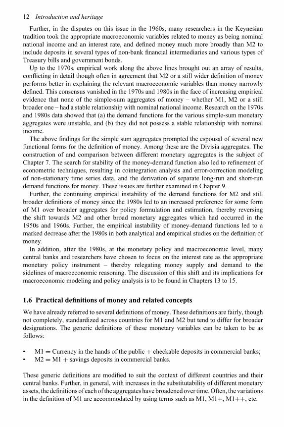
1.6 Practical definitions of money and related concepts
We have already referred to several definitions of money. These definitions are fairly, thoughnot completely, standardized across countries for M1 and M2 but tend to differ for broaderdesignations. The generic definitions of these monetary variables can be taken to be asfollows:
• M1 = Currency in the hands of the public + checkable deposits in commercial banks;• M2 = M1 + savings deposits in commercial banks.
These generic definitions are modified to suit the context of different countries and theircentral banks. Further, in general, with increases in the substitutability of different monetaryassets, the definitions of each of the aggregates have broadened over time. Often, the variationsin the definition of M1 are accommodated by using terms such as M1, M1+, M1++, etc.

Introduction 13
As an illustration of the variations in the various measures of money in practice in differentcountries, the following gives the current definitions of the major monetary aggregates inthe USA:
• M1 = currency in circulation among the public (i.e. excluding the Fed, the US Treasuryand commercial banks) + demand deposits in commercial banks8 (excluding interbankand US government deposits and those of foreign banks) + other checkable depositsincluding negotiable orders of withdrawal (NOW) + credit union (such as Savings andLoan Associations) share draft accounts + demand deposits at thrift institutions (suchas Mutual Savings Banks) – cash items in the process of collection and Federal Reservefloat;
• M2 = M1 + savings deposits, including money market deposit accounts + small timedeposits under $100,000 + balances in retail money market mutual funds;
• M3 = M2 + time deposits over $100,000 + Eurodollars held by US residents at foreignbranches of US banks and at all banks in the UK and Canada + money market mutualfunds held by institutions.
Note that M1, M2 and M3 exclude amounts held by US commercial banks, the USgovernment, money market funds, foreign banks and official institutions.
The above detailed descriptions for the United States of M1 and M2 are more complex thanour usual modes of defining them. However, our usual definitions are reasonable proxies.Under our proxy definitions, M1 is defined as currency in the hands of the public pluscheckable deposits in deposit-taking financial institutions. M2 is defined as M1 plus (smallor retail) time and savings deposits in these institutions.
For Canada, the monetary aggregates are measured as:
• M1 = currency in the hands of the public and demand deposits in chartered banks9;• M1+ = M1 + personal checkable deposits + non-personal checkable notice deposits at
chartered banks, mortgage loan companies and credit unions;• M2 = M1 plus personal savings deposits and non-personal notice deposits at chartered
banks;• M2+ = M2 plus deposits at trust and mortgage loan companies and credit unions
(including caisses populaires10);• “Adjusted M2+” = M2+ plus Canada Savings Bonds and mutual funds at financial
institutions;• M3 = M2 plus non-personal fixed-term deposits at chartered banks and foreign currency
deposits of residents booked in Canada.
For the United Kingdom, the definitions of the symbols in common usage are:
• M1 = currency plus current account (checking) sterling deposits in retail banks andbuilding societies, held by “UK residents”11;
8 Our usage of the term “commercial banks” refers to “depository institutions” in the USA.9 The chartered banks in Canada correspond to the commercial banks in our discussions.
10 These are essentially credit unions in Quebec.11 “UK residents” is meant to exclude the public sector and the financial institutions.

14 Introduction and heritage
• M2 = currency plus sterling deposits in retail banks12 and building societies, held byUK residents;
• M4 = currency plus sterling deposits at the central bank, other banks and buildingsocieties held by UK residents.
Note that the definitions of the monetary aggregates beyond M2, e.g. M3 and M4, differmore radically among countries than those of M1 and M2. For M3 and M4, the only commondenominator is that they are broader than M2 and include, besides M2, other highly liquidassets held at financial institutions. The reliance on these specific wider aggregates usuallyreflects the peculiarities of the country’s financial structure.
Note also that currency holdings and M1 are becoming increasingly smaller proportionsof M2 and wider aggregates. In the USA, at the end of 1995, the amount of currency in theeconomy was $379b13, M1 was $1150b, M2 was $3680b and M3 was $4954b. The ratio ofM1 to M2 was only 31 percent and to M3 was 23 percent. For Canada in 1995, the currencyin the economy was $26.8b, M1 was $62.7b, while M2+ was $618.4b The ratio of M1 toM2+ was only 10 percent. For the UK in 1995, currency holdings were £20.8b, M2 was£439.4b, and M4 was £682.5b.14
1.6.1 Monetary base and the monetary base multiplier
The money supply is related to the monetary base – sometimes called the reserve base – by themonetary base multiplier. Since this multiplier is greater than one, the monetary base is alsoknown as high-powered money. We will use the symbol M0 for it. Its generic definition is:
• M0 = Currency in the hands of the non-bank public plus currency held by the commercialbanks + reserves held by the commercial banks with the central bank.
The central bank can control the monetary base through open market operations and othermeasures, for which see Chapter 11. For any given definition of money, the “monetary basemultiplier” is defined as ∂M/∂M0. If the value of this multiplier is constant or a function of asmall set of variables, the central bank may be able to control the money supply by changingthe monetary base. However, our remarks in this chapter on the instability of the money-demand function in recent decades imply that this multiplier is definitely not a constant oreven a stable function of a small set of variables because of extensive financial innovation,so that the central bank’s control over the monetary base has not ensured a similar degree ofcontrol over the money supply.
The monetary base (to money) multiplier needs to be distinguished from the “money(to nominal income) multiplier,” which is defined as ∂Y /∂M , where Y is nominal nationalincome. Since Y ≡ MV , where V is the velocity of money (see Chapter 2), the moneymultiplier equals V . This multiplier is normally not a constant but, at the minimum, is afunction of several variables, including the interest rate. This function may, or may not be,also unstable.
12 Since 1993, these deposits include both non-interest-bearing and interest-bearing deposits.13 b stands for billion, defined as 1000 million.14 These figures are taken from Statistics on Payment Systems in the Group of Ten Countries, published by the
Bank for International Settlements, various years.

Introduction 15
Therefore, the central bank’s control over the monetary base need not ensure a high degreeof control over nominal income because of the instability of the monetary base multiplier orthe instability of the velocity of circulation of money, or both.
1.7 Interest rates versus money supply as the operating targetof monetary policy
Central banks may exercise control over the economy’s interest rates, in addition to themoney supply or, in its place, as their monetary policy instrument. Our concern at this pointis really with the instrument that is used as the primary one – that is, set exogenously by thecentral bank. If the money supply is used as the primary instrument, the economy’s interestrates will change in response to the central bank’s changes in the money supply, and willbe endogenous. If the interest rates are used as the primary monetary policy instrument, theeconomy’s money demand will change in response to the changes in interest rates. In thiscase, if the money market is to maintain equilibrium, the central bank has to accommodatethe change in money demand by appropriate changes in the money supply, so that the moneysupply will become endogenous. While the choice between the money supply and the interestrates can be trivial under certainty and a stable money-demand function, it is not likely to betrivial under uncertainty and an unstable money-demand function, so that central banks areforced to make choices between the two alternatives.
This issue has been brought to the forefront of the debate on the appropriate macroeconomicanalysis by the adoption by central banks in several developed economies of the policy ofusing the interest rate as the primary monetary policy instrument – and the abandonmentof this role for the money supply. Several new Keynesian models of the last two decadesnow incorporate such an assumption. This issue will be discussed in proper detail in thepresentation of these models later in this chapter and in Chapters 13 and 15.
1.8 Financial intermediaries and the creation of financial assets
Asset transmutation by financial intermediaries
Financial intermediaries are institutions that intermediate in the financial process betweenultimate borrowers and ultimate lenders in the economy. The ultimate borrowers include(a) consumers who need to borrow to finance part or all of their consumption, (b) firms thatborrow to invest in physical capital, and (c) the government when it borrows to finance itsdeficits. The ultimate lenders are the economic units that save part of their current incomeby spending less than their current income on their purchases of commodities and want tolend some or all of these savings to others for some duration. Householders form the majorbulk of the ultimate lenders, saving part of their current income. Some of the firms engagedin production also do not spend all of their sales revenue on immediate purchases of inputsor distribute them to shareholders as distributed profits but save part of them (i.e. keepingsome profits as retained earnings). They are sometimes willing to lend part of these retainedearnings to others. The government does the same on a net basis when it runs a surplus.
Financial intermediaries borrow from the ultimate lenders or from other intermediariesby issuing their own liabilities in exchange and re-lend to others by accepting the latter’sliabilities. In the modern economy, only a small proportion of the savings is directlytransferred from the savers to the ultimate borrowers. Most of the savings are directed bythe savers to financial intermediaries such as banks, mutual funds, pension funds, insurance

16 Introduction and heritage
companies, etc., which re-channel the funds thus obtained to firms and the government, eitherdirectly by buying their shares and bonds or indirectly through other financial intermediariessuch as investment banks.
The basic reason for this intermediation is the differences in the preferences of thesavers for asset characteristics, such as liquidity and security, and those attaching to theinstruments issued by the firms and the government. Consequently, there is in general aconsiderable difference in the characteristics of the liabilities sold to the savers by a financialintermediary and those of the assets bought by it, resulting in what is sometimes called theasset–transmutation process.
Banks are financial intermediaries that borrow from the public by inviting demand andtime deposits or issuing their own securities and hold the liabilities issued by others. Theirexistence is a superb example of asset transmutation through financial intermediation. Themain liabilities of banks are deposits which are virtually riskless to the depositors since theyare payable on demand or after a short specified notice. In short, they are highly liquid.By contrast, the assets held by the banks are government securities, loans to the public,etc., possessing some risk of loss and, as with loans, a limited degree of marketability orencashment at short notice. Therefore, the assets issued by the banks are much more liquidthan the assets held by them. Conversely, the return paid by the banks on the former is lessthan the return that the banks earn on the latter.
Multiple creation of financial assets
All financial assets are “created” and have no intrinsic physical existence, but are the liabilitiesof some economic unit or other. They may be examined in terms of their characteristics,especially in terms of their yield or expected yield, risk of loss, marketability, maturity andso on. Anyone purchasing a financial asset may be thought of as purchasing a particular set ofcharacteristics, such as risk and marketability etc., in exchange for a specified expected yieldon the asset. Financial intermediaries cater to this demand through the creation of assets withdiffering combinations of characteristics. For many pairs of assets, it is feasible for someintermediary to create a third asset that offers a mix of the characteristics of the original twoassets, so that the multiplicity of differentiated assets is a common outcome of unregulatedfinancial intermediation.
Financial intermediaries typically issue assets with more desirable characteristics forlenders than do the ultimate borrowers, persuading the latter to hold the liabilities of theintermediaries. In turn, the intermediaries use the funds obtained from the sale of theirliabilities to purchase the liabilities of other borrowers which pay a higher expected netyield, thus covering the expenses of intermediation and making a profit in the process.
Financial intermediaries permeating an unregulated economy lead to a multiplicativecreation of their liabilities. To illustrate, consider an economy in which everyone is willing tohold the asset A issued by a given intermediary.15 Now assume that an ultimate lender saves$100 and exchanges it for the asset A. The intermediary transfers (lends) the $100 to anotherindividual B, who transfers them in some way, such as through consumption or investmentexpenditures, to a third individual C. The last individual again exchanges the $100 of fundsfor the assets issued by the intermediary. Suppose these are the only transactions that takeplace in a given period and there are no leakages at any point. Then, the intermediary, for an
15 For example, deposits in a bank.

Introduction 17
initial $100 lent to it, has created $100 of its liabilities. The amount created over n periods willbe $100n and will approach infinity over time. The implication of this example is clear: themultiplicative creation of the liabilities of financial intermediaries is inherent in an economyin which these liabilities are widely held. The extent of this creation is limited by the leakagesout of the recycling process. Thus, if individual C had only deposited $50 of resources withthe intermediary and retained the remainder in his storage, the recycling process would havehad a leakage of $50 (or 50 percent). The total assets created by the intermediary in the periodwould be worth only $50 and only $100 over time.
Banks conform to the above pattern. The funds they receive are deposits of currency andare part of their reserve base. They lend these out, after keeping some of this currency to meettheir own demand for reserves, part of which they are in some countries legally required tokeep. The public receiving the funds may, after some transfers within its own members oreven without any transfers, redeposit the funds in the banks. It may also retain some currencyto meet its own demand for it. The remainder returns to the banks and starts the next cycleof the asset–creation process. The leakages in the form of the currency demand of the publicand of the banks against their deposits prevent an infinite creation of deposits over time butnevertheless lead to some multiple expansion of the banks’ liabilities, unless the leakageswere 100 percent in the first cycle.
Since financial assets are created, it is natural to expect that in an unregulated system avariety of financial assets differing only slightly in their characteristics and with varyingdegrees of closeness of substitution will come into existence. Further, any regulation ofexisting assets tends to increase the profitability of unregulated potential substitutes andusually leads to their creation. These tendencies towards multiplicity of financial assetsintroduce severe problems in defining money and in its regulation. Further, the financialdevelopment of a country is usually marked by the increasing richness of the financial assetsavailable in it and the increasing closeness of near-money assets with the asset that serves asthe medium of payments. Consequently, questions on the proper definition of money neverseem to die out, thereby posing a continual challenge to monetary economists to appropriatelyredefine money.
Distinctive role of banks as financial intermediaries
Banks are not the only financial intermediaries in the economy. But they are the mostwidespread and their liabilities are so widely demanded that the multiple creation of theirliabilities is both the greatest and the most widely recognized. Banks, accepting demandand time deposits, differ from other financial intermediaries in that their liabilities are readilyacceptable and are liquid since demand deposits are a medium of payments and hence a form ofmoney. Further, another of their liabilities, time deposits, is a very close substitute for currencyand demand deposits. By comparison, the liabilities of non-bank financial intermediaries arenot directly a medium of payments, nor are they perfect substitutes for it. This special role ofthe liabilities of banks in the economy makes the banks a rather distinctive type of financialintermediary and makes a study of their behavior and reaction to monetary policy especiallyimportant.
Fragility of the financial system
The financial system is said to be fragile in the sense that it is prone to crisis. The reasonsfor this include banks’ reliance on fractional reserves and asset transmutation. Since they

18 Introduction and heritage
hold only a small part of their liabilities, mainly deposits, in reserves (currency holdings anddeposits with the central bank), they are not able to refund these deposits if the depositorswish to suddenly and simultaneously try to withdraw a considerable fraction of deposits.Such a withdrawal from a bank is known as a “run” on the bank and its most visiblemanifestation is long lines of depositors waiting to enter the bank to make their withdrawals.Asset transmutation means that banks’ liabilities have a much shorter maturity than theirassets. In the case of a run on the bank, if the bank tries to sell its assets at short notice itis likely to incur a loss over the amount that it would get if it held the assets to maturity orcould sell them at a more opportune time. Also, note that a considerable part of the assetsheld by banks are in the form of non-marketable loans, which are difficult to convert intocash at short notice.
Therefore, the fractional reserve system, with its asset transmutation, rests on trust by thedepositors in the continuing liquidity and solvency of the bank in question. The emergenceof less than absolute trust in the bank’s ability to honor withdrawals from it, even if this isdue to an unjustified rumor or just contagion spreading from other financial institutions, canbe enough to trigger a run on it, as well as a refusal by other financial institutions to cometo its aid and lend to it. This can soon result in closure of the bank. Some protection againstsuch an eventuality is provided by insurance of its deposits, often by a public agency, so thatdepositors do not need to worry about the safety of their deposits, and by the central bank’sdoctrine of “lender of last resort.” Under the latter, even if no private lender will lend to thebank, the central bank will do so. These issues are covered in Chapter 11 on central banking.
1.9 Different modes of analysis of the economy
Since the money market is only one of the markets in the economy, monetary economicsis closely intertwined with the analysis of the other markets in the economy. This unifiedanalysis of money and all other markets in the economy can be conducted in one of two ways:
(I) A microeconomic analysis of the market for each of the goods in the economy. Whilethere can be different types of such models, many of them are made analytically tractableat the level of the economy by imposing the assumptions of perfect markets (perfectcompetition and instant market clearance), absence of market imperfections such asfrictions and transactions costs, etc., on the analysis of each market. Other types ofmicroeconomic models discard one or more of these assumptions for selected markets.
Microeconomic models of the economy assuming perfect competition are calledWalrasian models. They are difficult to manage unless the assumption of equilibrium –that is, demand equal to supply – in all markets is imposed on them. The (subsidiary)group of Walrasian models that does so provides microeconomic models of the economyknown as the Walrasian general equilibrium models. Given the assumptions of perfectcompetition, absence of frictions, transactions costs and uncertainty, as well as generalequilibrium in all markets, including the labor market, such a model implies that, inthe general equilibrium state, money is neutral, that is, changes in the money supplydo not alter the values of the real variables, including employment and the outputof commodities. This equilibrium is usually called the “long-run state” of the model.However:
(i) Money is is not neutral in most specifications, in cases where they are spelled out,of the disequilibrium or the short-run equilibrium states of the Walrasian models.

Introduction 19
(ii) Money is not neutral even in the equilibrium of those models that dispense with oneor more of the assumptions listed above. Such states are often labeled as “short-run”equilibrium ones. For instance, it is not neutral in short-run equilibrium if there isuncertainty and errors in expectations, or if the markets are not perfect, or if frictionsand transactions costs exist.
(II) A macroeconomic analysis, where the goods are classified into a small number ofcategories and the analysis is performed at this composite level. Although manydifferent ways of categorizing goods are possible, the one generally used in short-runmacroeconomics is that of classifying goods for the closed-economy analysis into thefour categories of commodities, money, bonds (non-monetary financial assets), and labor,and that of open-economy analysis into the above four goods and foreign exchange.
The relationship between the microeconomic and the macroeconomic varieties of modelscan be either:
(A) (II) is merely a compact form of (I). In this case, the assumptions and implications ofmacroeconomic analysis must be consistent with the microeconomic analysis of markets.This approach seeks to set the foundations of macroeconomics in microeconomic theory.Note that doing so will only embody whatever features the underlying microeconomicmodel possesses. Therefore, if the underlying model possesses nominal wage and/orprice rigidities or allows the absence of instantaneous market clearance, so will thederivative macroeconomic model.16 If the model assumes the absence of nominal wageand price rigidities and instant market clearance, so will the derivative model.17
(B) (II) is different from and possibly more insightful than just being a compact formof (I). In this case, in addition to the assumptions on the individualistic behavior ofeconomic units, macroeconomic models can incorporate assumptions that deal withgroup behavior,18 as well as interactions among markets19 and groups20 that are notvisible in microeconomic analysis. If these are relevant, macroeconomics providesthe guide for the specification of the appropriate microeconomic analysis, so thatmacroeconomics serves as the foundation for the relevant microeconomics. Further,models of type (II) are often more tractable for studying the properties of the economyin disequilibrium or if there exist departures from perfect competition.
Each of the above types of analysis has its advantages and disadvantages. The advantage of(A) is that it roots macroeconomic behavior in the microeconomic analysis of the householdand firm, which provides a check on the rationality of the assumed behavior of households andfirms. However, there are two major disadvantages to using (A). One of these is that it usuallyextends the assumption of continuous equilibrium to all markets, thereby usually assuming
16 New Keynesian macroeconomic models of the last two decades are usually of this type.17 Modern versions of the classical school tend to be of this type.18 For example, a “herd instinct” (such as contagion, panic and euphoria in stock markets) may be important when
studying the behavior of groups but not when studying the behavior of any one economic agent. While theexistence of herds is intuitively obvious, its formal modeling is still at an early stage.
19 For example, spillovers between markets can be quite important between the labor market and the commoditymarket – such as the fact that unemployed workers reduce their consumption of commodities – while they tendto be ignored in the microeconomic analysis of individual economic agents and markets.
20 E.g. labor unions and firms’ cartels.

20 Introduction and heritage
that all markets are simultaneously, and always, in equilibrium. While such an assumptionseems quite sensible and may be relatively innocuous at the level of one market, it is oftennot a sufficiently valid assumption for the whole economy. In particular, the assumptionof simultaneous and instantaneous equilibrium prevents the study of the elements of thepathology of the system,21 i.e. when some part of it breaks down, so that the overall systemdoes not possess general equilibrium, possibly not even the ability to return to it soon inreal time.22 The other major disadvantage, as mentioned above, of purely microeconomicanalysis is that it tends to ignore behavior that is applicable only in the mass or in groups butnot to individual economic units studied in isolation.23
The Walrasian general equilibrium system provides the benchmark of the well-functioning,healthy economy. It is extremely useful in this respect and remains central to the studyof macroeconomics. Among the major components of this system are: a complete set ofmarkets for all possible goods, utility maximization by consumers and workers and profitmaximization by firms,24 perfectly competitive and perfectly efficient markets,25 certaintyor the absence of errors in expectations, absence of barriers to the attainment of equilibrium,absence of lags and “false trading,”26 and the availability of a mechanism for instantlyreaching the general equilibrium for the economy.27 This is indeed a tall set of assumptionsand economists use them mainly for deriving implication for the analytical long-run state ofthe economy. They approach the short-run as a minor deviation from the long-run model.Macroeconomic models of this type are the “classical” group of models. They belong tocategory (A) above.
The Walrasian general equilibrium system, incorporating perfect competition and perfectefficiency, by its very nature, does not provide an appropriate platform for studying thepathology of the economy when it is not functioning well in whole or in some of its parts.Their main rival is the Keynesian group of models, which focus on the pathology of theeconomy to specify the short-run analysis of the economy, with the long-run model becominga variation on short-run modeling. Keynesian models belong to category (B) above.
1.10 The classical paradigm: the classical groupof macroeconomic models
The classical group of models is consistent with the Walrasian general equilibrium frameworkand assumes that the market establishes the wages and prices for each of the goods at that
21 A comparison of the economy with the human body can illustrate this point. The human body does not alwaysstay healthy. Further, if it gets sick, it may be able to recover back to good health but may not do so soon. Hence,modeling (studying) only the properties of the healthy body may provide poor or disastrous recommendationsof what treatment to administer when it does become ill.
22 Here, the chronological time taken to reach the general equilibrium state is of the essence, so that the propertiesof long-run equilibrium are of little consequence unless the chronological time taken to reach the long-run isalso specified.
23 Note that neither of these disadvantages resorts to an appeal to irrational economic behavior. Additionally, ifbehavior is, in fact, non-rational, then a model which excludes such behavior would not capture reality.
24 Under uncertainty, these would become expected utility maximization by both households and firms.25 Markets are perfectly “efficient” if they instantaneously restore equilibrium following a shock to demand and/or
supply. Note that this is a different assumption from that of perfect competition, which is defined as the state inwhich no buyer or seller can influence the market price.
26 That is, trading at prices and quantities other than those that will occur in equilibrium.27 These are often presented under the rubric of the Arrow–Debreu model, which is a rigorous statement of the
Walrasian general equilibrium model.

Introduction 21
level at which its notional demand and supply are equal (i.e. at which its market “clears”).Since one of the markets is labor, its clearance implies that every worker who wishes tosupply labor at the existing wage will have a job and each firm will be able to employ allthe workers that it wants to at the existing wage. This state, in the context of the long-runanalysis, is known as “full employment,” so that a hallmark of the classical models is that,in long-run equilibrium, they imply full employment.28 However, in view of their emphasison labor market clearance, this implication of equilibrium is often turned around and statedas if it was an assumption, which is not strictly correct.29
While there is no consensus on the division of the classical group of models into individualmodels, we adopt the following taxonomy for this book.
I. Traditional classical ideas
“The traditional classical approach (or ideas)” is being proposed in this book as the namefor the somewhat disparate ideas on the macrostructure of the economy from the middleof the eighteenth century to the publication of Keynes’s The General Theory in 1936. Toquite a considerable extent, these ideas were diffuse, varied among authors and changed overtime. In any case, there was no single compact version of the overall exposition, though theprofession, following Keynes, now treats them as if there was a compact model. We willcall this compact statement of the traditional classical ideas the traditional classical model. Itwas never stated as a compact model even during its heyday during the nineteenth and earlytwentieth centuries, but its ideas permeate the classical paradigm.
The two components of the traditional classical model directly relevant to monetaryeconomics were the quantity theory for the determination of prices (see Chapter 2) andthe loanable funds theory for the determination of interest rates (see Chapter 19). Its theoryof employment was the analysis of the labor market and incorporated the assumption ofequilibrium, which state represents full employment, so that the traditional classical set ofideas did not possess a theory of unemployment or of variations in aggregate employmentother than those of variations in their long-run levels. Hence, it did not possess a theory ofthe deviations in unemployment and output from their full-employment levels. However,another component of the traditional classical ideas was its business cycle explanations,which allowed for fluctuations in economic activity in the economy’s response to real ormonetary shocks, so that such explanations implicitly did envisage deviations from fullemployment.
The traditional classical approach lacked the integration of its microeconomic-based theoryof employment and output with its business cycle explanations, as well as of their mix withthe quantity theory and the loanable funds theory. To sum up, while this approach had manyof the components of macroeconomics, it lacked an integrated macroeconomic framework. Italso lacked an explicit treatment of the aggregate demand for commodities, now encompassedin the IS relationship, which is an essential building block of current macroeconomics.
28 In the short-run of the classical models, with errors in expectations, market clearance can imply a level ofemployment different from the full-employment (long-run equilibrium) level.
29 The difference between an assumption of full employment and one that is an implication of the equilibriumstate is that the former rules out the studies of the properties of the system when it is in disequilibrium; the latterdoes not necessarily do so. In addition, the former can rule out a distinction between short-run and long-runequilibrium.

22 Introduction and heritage
THEORY OF AGGREGATE DEMAND IN THE TRADITIONAL CLASSICAL APPROACH AND SAY’S LAW
There was also no explicit macroeconomic theory of the commodity market in the traditionalclassical approach since it did not incorporate a theory for the determination of the aggregatedemand for commodities.30 Instead, this approach studied each commodity market separatelyin microeconomic terms, that is, in terms of its demand and supply analysis. In place of atheory of aggregate demand for commodities as a whole, the traditional classical approachexplicitly, but more often implicitly, settled for Say’s law (see Chapter 18), which stated that,in the aggregate, the supply of commodities creates (i.e. always generates) its own demand,so that a separate theory of aggregate demand was not needed or specified.
Say’s law was pervasive in the analyses offered by many economists throughout theclassical period: among others, it was espoused by Adam Smith in the eighteenth century,David Ricardo in the early nineteenth century, John Stuart Mill in the mid-nineteenth centuryand Alfred Marshall in the late nineteenth century. However, Say’s law is not valid for amonetary economy, which possesses commodities, money and bonds, for several reasons.One of these is that, in a monetary economy, all sellers of commodities are not automaticallybuyers of commodities to the same extent, since a part of the income of sellers is usuallysaved, which can be put by them into money or bonds (which include savings deposits inbanks) rather than being automatically converted into spending on commodities.
Note that modern theories of aggregate demand do not embody Say’s law, so that it is nolonger a part of modern macroeconomics.
II. Neoclassical model
The “neoclassical model” is the name given to the restatement of the traditional classical ideasrebottled and re-flavored in the post-General Theory period in a new compact framework. Thenew bottle was the IS–LM framework of analysis; the re-flavoring included the elucidationof some of the nuances of the traditional classical ideas, such as the wealth/Pigou and realbalance effects (see Chapter 3) on commodity demand, as well as the addition of new elementssuch as the speculative demand for money (see Chapter 5) and the explicit analysis of thecommodity market at the macroeconomic level. Further, certain elements of the traditionalideas such as the quantity theory, the loanable funds theory, Say’s law and the dichotomybetween the real and the monetary sectors of the economy were discarded in the rebottlingprocess. The resulting model also differed from the traditional classical ideas by being anintegrated macroeconomic framework.
The classical paradigm was, in general, rejected by the majority of the economics professionfrom the 1940s to the 1970s, though it continued to exist as an outcast. However, refinementsand additions to it continued to be made during these decades. The dominant paradigm in thesedecades was the Keynesian one. The classical paradigm, though with new models, roaredback in the 1970s and has since then taken various forms. These are the 1970s monetarism,the modern classical model and the new classical model.
III. 1970s monetarism
The 1970s monetarist approach, also known as the St Louis monetarism, was the name givento a mainly empirical analysis whose empirical and theoretical expositions were initiated
30 The analysis of aggregate demand requires the concept of the multiplier, which was proposed only in the 1930s.

Introduction 23
by economists at the Federal Reserve Bank of St Louis during the 1970s. The short-runversion of their model did not assume full employment and did not imply continuous fullemployment in the economy. It was relatively close to the then Keynesian models in terms ofthe impact of monetary policy on output and employment, but it denied on empirical groundsthe Keynesian claim of the efficacy of fiscal policy. In its long-run version, it belonged in theclassical paradigm.
Therefore, the 1970s monetarism was a hybrid between the classical and the Keynesianparadigms, and made the switch away from Keynesianism palatable for many economists.However, it did not propose any fundamentally new theories, had a short life and was replacedin the early 1980s by ideas truer to the classical paradigm, which eventually took the formof the modern classical paradigm.
IV. Modern classical model
The modern classical model is a statement of the classical paradigm under the assumptions,among others, of continuous labor market clearance even in the short-run, which had strictlynot been part of the neoclassical model. In addition, for the short-run, this approach extendsthe neoclassical model by the introduction of uncertainty and rational expectations. In manyrespects, the modern classical approach is closer to the Walrasian general equilibriummodel than to the traditional classical and neoclassical approaches. It is currently thedominant component of the classical paradigm. Its foundation was laid during the 1970sand 1980s.
For the long-run, the modern classical model extends the definition of the (analytical)long-run to include, in addition to the absence of any adjustment costs and rigidities, theassumption that there are no errors, even random ones, in expectations, which is tantamountto the assumption of certainty. Given labor market clearance, this long-run state is the full-employment one.
For the short-run, the modern classical model allows uncertainty, but with expectationsformed according to the rational expectations hypothesis. A discussion of the modern classicalmodel appears in Chapter 14. Among its major implications is that deviations from fullemployment will occur if the expected price level is different from the actual one, so thatthere are errors in expectations. However, these errors will be random, and by their very natureare transient and self-correcting, so that the short-run deviations from full employment willbe transient and self-correcting. In this context, systematic monetary and fiscal policies donot change output and unemployment in the short, as well as the long, run. Further, there isno need for such policies since the economy has the ability to go to full employment on itsown and within a short period.
Note that, because of the assumption of continuous labor market clearance both in the short-run and in the long-run, involuntary unemployment31 cannot exist in the modern classicalmodel, even when there are short-run deviations of employment from the full-employment(long-run equilibrium) level.
The modern classical model has serious limitations. In particular, it does not offer asatisfactory explanation for the short-run stylized facts (listed later in Section 1.12) on theimpact of shifts in monetary policy on output (see Chapter 14).
31 Involuntary unemployment requires that labor demand exceeds labor supply at the given wage.

24 Introduction and heritage
Briefly, for the long-run, the modern classical model is a compact form of the Walrasiangeneral equilibrium model, so that its implications are consistent with those of the latter.It provides the benchmark conclusions, consistent with the stylized facts, on the long-runrelationship between money and output. For the short-run, the modern classical modelproduces transient and self-correcting deviations from full employment, so that there is nosensible role for systematic monetary and fiscal policies in both the short-run and the long-run. For the short-run, the implications of the model for output and unemployment are notvalid.
V. New classical model
The new classical model imposes the assumption of Ricardian equivalence on the modernclassical model. This assumption is an aspect of intertemporal rationality and the Jeffersonian(democratic) notion that the government is nothing more than a representative of its electorateand is regarded as such by the public in making the decisions on its own consumption. Sucha government is taken to provide just the goods that the population wants and its bonds,held by the public, are regarded by it (the public) as a debt owed by the public to itself.The implications of these assumptions are that the public debt is not part of the net worth ofthe public and that the public increases its private saving by the amount of a bond-financedgovernment deficit. The latter implies that such deficits do not affect aggregate demand inthe economy, and therefore do not change nominal or real GDP (see Chapter 14 for thisanalysis).
Of all the macroeconomic models in the classical paradigm, the new classical model is themost restrictive one because of its assumption of Ricardian equivalence.
The major alternative to the classical paradigm is the Keynesian one, which has its ownset of models.
1.11 The Keynesian paradigm and the Keynesian setof macroeconomic models
Using the analogy between the economy and the human body
The fundamental difference between the classical and Keynesian paradigms is that while theformer focuses on the healthy state of the economy,32 the latter focuses on the pathology –especially the system-wide pathology – of the economy,33 which may not fully or soonrecover34 from a shock to it (Solow, 1980, 1991). The Keynesian paradigm recognizes thatthe economy may sometimes have equilibrium in all markets, but does not assert that thisoccurs always or most of the time. Further, even if there is equilibrium, it may not be thecompetitive equilibrium of the Walrasian general equilibrium model because the economymay have a different structure or because of group behavior. As a consequence, the Keynesianparadigm implies that when the economy is outside the Walrasian general equilibrium, thegovernment and the central bank may be able to improve on its actual performance throughtheir policies.
32 That is, with clearance of all markets.33 That is, when the economy is thrown out of equilibrium.34 That is, return to equilibrium in all markets.

Introduction 25
We have at various places drawn an analogy between the equilibrium state of theeconomy and the healthy state of the human body, and that between the deviations fromequilibrium and the pathology of the human body. The human body sometimes functions inperfect health and sometimes suffers minor illnesses of a brief expected duration and withoutany need for the help of a professional (doctor). But it could sometimes suffer from seriousillnesses from which the recovery may occur but be slow and be speeded up by the helpof a doctor, or suffer ones from which there is no recovery without the intervention of aspecialist. There may also be illnesses from which there is no cure and no recovery, but wedo not include this limiting state within our analogy. Among the serious illnesses, we notethere can be many possibilities: infection with bacterium A rather than B, infection by abacterium versus a virus, an infection versus a collapse of a lung, a collapse of a lung ratherthan a heart attack, etc. The list of the possible sources of the deviations from the healthystate can be endless.
Comparing the approach of the two paradigms to the pathology of the economy andapplying our analogy, when the classical paradigm does envisage deviations away from thehealthy state of the economy, they are supposed to be minor, transitory and self-correcting.Under it, while the economic body may become ill (that is, deviate from the full-employmentstate), the illnesses are never serious or long lasting, so that a trip to a doctor either neverbecomes necessary or will not really be worth the hassle and the cost. By comparison, theKeynesian paradigm envisages the possibility of more serious departures from the generalequilibrium (healthy) state of the economy. Its deviations from equilibrium can be due todifferent pathogens or breakdowns of the different components of the economy. Further, itallows for the possibilities that the recovery may be slow and could be speeded up with experthelp (from the government and the central bank), or that it may never occur without such help.
Using the analogy with the human body, we offer the following two fundamental – andhighly plausible – axioms on the performance of the macroeconomy.
α. The economy, like the human body, may sometimes function well and sometimes not.
Hence, it is essential to study both states, with the former serving as the benchmark for thetreatment of the latter.
β. When the economy, just like the human body, is not functioning properly, the causes,symptoms and effective treatments of the malfunction can be quite varied.
The justification for the β axiom is that one cannot plausibly attribute all possibleillnesses to a single underlying cause or attribute all potential causes to an overarching singlesource. An implication of the β axiom is that since the Keynesian paradigm focuses on thepathology of the economy, it cannot properly be encapsulated within one model with one rootpathogen. Hence, more than the classical paradigm and its models, which are almost linearor hierarchical in their relationship, the Keynesian paradigm, if it is to do its job properly,has to be a disparate and, at best, a rather loose collection of models.
To reiterate, by the nature of their attempts to deal with the pathology of the economy,the Keynesian models have to be, and are, quite varied. If they are to do their job properlyof dealing with the different types of deviations, such models need not – in fact, must not –all focus on the same types of deviation from the overall equilibrium state or make the samerecommendations for policies to address these deviations. Unfortunately, this aspect of theKeynesian paradigm is often not recognized. Frequently, the presentations and discussions
26 Introduction and heritage
of the Keynesian models miss this requirement for variety within the Keynesian paradigmand seek to force the various Keynesian models into a single format or view it as one unifiedmodel. The danger in doing so is that a single prescription could be given as a cure-all forvery disparate causes and be inappropriate for many.35 Chapter 15 provides a small numberout of the variety of Keynesian models in the literature.
Frequent themes in the Keynesian models
A common concern of the Keynesian models is with the potential for involuntaryunemployment, which produces deviations of actual employment from its full-employmentlevel. Consequently, these models tend to pay special attention to the structure of the labormarket, its demand and supply functions and whether or not equilibrium holds between them.Within this focus, many Keynesian models assume nominal wage rigidity, often justified bytheories of nominal wage contracts between the workers and the firms. However, there arealso Keynesian models that consider the deviations from general equilibrium that could occureven when the nominal wage is fully flexible.
The assumption of the rigidity or stickiness of prices in the economy is often regarded asanother common theme of Keynesian models. While this assumption can impose deviationsfrom a general equilibrium, it need not be the only cause of or reason for potential deviations.Therefore, models within the Keynesian paradigm need not, and should not, all be based onprice rigidity. There is, consequently, also a place for Keynesian models that consider thedeviations from general equilibrium that could occur even when the prices are fully flexible.
Chapter 15 provides a look at some of the Keynesian models. While some of the modelspresented there assume equilibrium in the macroeconomic models, others do not do so. Whilesome assume a special form of the labor supply function, others assume a different form.While some assume – or imply on the basis of nominal wage contracts – nominal wagerigidity of some form, others do not do so. Similarly, while some models assume or implyprice level stickiness or rigidity, others do not do so. This variety in modeling within theKeynesian paradigm becomes even more evident when the Keynesian and the neoKeynesianmodels are compared.
To reiterate, the variety of modeling, though perplexing and sometimes seeminglycontradictory, in the Keynesian paradigm is essential to the proper study of the pathology ofthe economy. It would be a mistake to force the Keynesian models into a single straightjacket,even though this would provide an attractive means of comparing the classical and Keynesianparadigms as a whole.
1.12 Which macro paradigm or model must one believe in?
While most textbooks and economists would consider this to be a legitimate question, ourremarks above suggest that it is an improper, and quite likely a dangerous one, for the
35 An example of this is the economists’ inappropriate policy prescriptions, based mainly on traditional classicalideas, during the early stages of the Great Depression in the 1930s. These worsened the depth of the fall in GDPand lengthened the depression – and contributed to the demise of faith in the traditional classical ideas. Anotherexample of inappropriate policies, based on the aggregate demand management approach in the Keynesianparadigm, occurred in response to the supply shocks of 1973 and 1974. This led to stagflation and contributedto the demise of faith in the Keynesian paradigm.

Introduction 27
formulation of economic policies. The proper study of the economy requires the study ofboth its healthy state and its diseases. Since we cannot be sanguine that the economy willalways operate in general equilibrium, the models of the Keynesian paradigm must not beneglected. Since we cannot be sure that the economy will never be in general equilibrium,the models of the classical paradigm must also not be neglected. Both paradigms have theirrelevance and usefulness. Neglecting either of them can lead to erroneous policies that imposehigh costs on the economy and its citizens.
For the practical formulation of monetary policy, the relevant and “interesting” questionis not the a priori choice between the classical and the Keynesian models, but rather theperpetually topical one: what is the current state of the economy like and which model ismost applicable to it? There is rarely a sure answer to this question. Consequently, thejudgment on this question and the formulation of the proper monetary policy are an art,not a science – and very often rest on faith in one’s prior beliefs about the nature of theeconomy.
While one cannot dispense with one’s beliefs and economists rarely give up theirconception of the nature of the economy, the fundamental role of economics must be kept inmind. This is that economics is a positivist science, with the objective of explaining the realworld. This is done through its theories, which, by their very nature, must be simplifications –more like caricatures – of reality. As such, they may be valid or not, or be better for explainingsome aspects of reality rather than others. Intuition and econometrics are both needed anduseful in judging their validity and relative value. In brief, one should not hold a dogmaticbelief in one theory for all purposes.
A side implication of the positivist objective of economics is the normative one – i.e.the ability to offer policy prescriptions to improve on the performance of the economy,hopefully as a means of increasing the welfare of its citizens. Both the Keynesian and theclassical paradigms are essential to these roles.
One way of judging the extent to which the macroeconomic theories are valid or applicablefrom a monetary perspective is to compare their implications with the stylized facts of theeconomy.
Some stylized facts on money and output
Stylized facts on the relationship between money and output are general conclusions aboutthis relationship, established on the bases of intuition and empirical studies. Some of theseare:
1 Over long periods of time, there is a roughly one-to-one relationship between the moneysupply and the price level.
2 Over long periods of time, the relationship between inflation and output growth is notsignificant.
3 Over long periods of time, the correlation between money growth rates and nominalinterest rates is very high.
4 Changes in money supply and interest rates have a strong impact on aggregate demand.5 Over short periods (a few years), increases in aggregate demand, because of increases
in money supply or reductions in interest rates, increase output. This effect builds to apeak and then gradually decreases, so that there is a “hump-shaped pattern” of the effectof monetary policy on output, with the maximum increase in output occurring with a laglonger than one year, sometimes two or more years.

28 Introduction and heritage
6 The impact of an expansionary monetary policy on prices occurs with a longer lag thanon output, so that the impact of monetary shocks on output does not mainly occur throughprice movements.
7 Contractionary monetary policies initially reduce output significantly, often for longerthan a year and sometimes for several years. The cost in terms of output tends to belarger if inflation is brought down gradually rather than rapidly. It is lower if the policyhas greater credibility.
Using analytical terminology, money is not neutral in the short-run but is neutral in thelong-run. These conclusions hold for monetary policy, whether it changes the money supplyor interest rates. Chapter 14 provides a more detailed list of the stylized facts on the impactof monetary policy on output.
1.13 Walras’s law
For the closed economy, the standard models of the two paradigms assume four goods:commodities, money, bonds (i.e. all non-monetary financial assets) and labor. Therefore, thereshould be four equilibrium statements, one for each of the four goods, and the correspondingfour curves in the diagrammatic expositions. However, Walras’s law (see Chapter 18) ensuresthat equilibrium in any three out of the four markets implies equilibrium in the fourth one, sothat one of the markets need not be explicitly studied. This allows the diagrammatic expositionto work with only three equations/curves. Current macroeconomic analysis usually doesso for those of the commodity market (the IS equation/curve), the money market (the LMequation/curve if money supply is the instrument of monetary policy but the IR equation/curveif the interest rate is the instrument of monetary policy) and the aggregate supply function(AS equation/curve) or, in its place, a price–output adjustment equation, as in Chapters 14and 15. In this procedure, the bond market is the one excluded from explicit analysis, sothat the bond market curve is not usually drawn. It does, however, remain implicitly in theexposition and can be deduced from the other curves.36
1.14 Monetary policy
The standard assumption of monetary analysis was that the central bank exercises controlover the economy by exogenously controlling the money supply. In this case, the appropriateanalysis of aggregate demand is called IS–LM analysis, since the analysis of the moneymarket generates the IS equation/curve. However, for certain types of economies, controllingthe economy’s interest rate may be a surer way of controlling aggregate demand than itsmoney supply. The central banks of several developed economies, including those of theUnited States, Canada and Britain, now seem to rely more on the interest rate rather than onthe money supply as the primary monetary policy instrument.37 For their economies, the LMcurve is not appropriate. Instead, the analysis generates an IRT (interest rate target) curve,which, in addition to the IS curve, determines the aggregate demand in the model. The IS–LMand IS–IRT analyses are set out in Chapter 13.
36 This is done in Chapter 19.37 This is also so for the European Central Bank, which claims to treat the interest rate as its primary monetary
policy instrument but also monitors monetary aggregates.

Introduction 29
If the central bank sets the interest rate as its exogenous monetary policy instrument,it must be willing to supply the amount of money demanded at that interest rate. It cando this by appropriate changes in the monetary base, either of its volition or by allowingcommercial banks to borrow from it. In this case, the money supply becomes endogenous tothe economy.
1.15 Neutrality of money and of bonds
Neutrality of money (and credit/bonds) is the proposition that changes in the money supplyand monetary policy do not alter output and employment, as well as the real values of manyother real variables. For the short run, most models do not imply neutrality. However, asChapters 13 to 15 show later, the reasons for such non-neutrality differ between the twoparadigms and often also among the models of each paradigm. Note that in the long-runanalyses of most models, whether in the classical or the Keynesian paradigm, money andcredit are neutral, which is consistent with the stylized facts on the economy set out in Section1.12 and also in Chapter 14.
Money and credit (non-monetary financial variables) are usually not neutral in the shortterm in real-world economies. Sudden shifts in the availability of money and credit are amongthe most important reasons for fluctuations in output and unemployment. Notable examplesof such non-neutrality are provided by currency, credit and exchange crises, which originatein the financial sector and spread to the real sectors of the economy.
An illustration: the subprime crisis of 2007 in the USA
The “subprime crisis” originating in the United States in 2007, and its impact on the realsectors of the US and world economies, provide a compelling illustration of the non-neutrality of both money and credit in the economy. Subprime loans in this context wereloans made as mortgages to borrowers who were poor credit risks in terms of their incomesand the collateral that they could provide. However, when house prices were rising sharply,such mortgages seemed to be a good bet for both borrowers and lenders. House pricesrose sharply from 2002 to 2006, at some point becoming a “bubble.”38 These mortgageswere bundled into “asset-backed corporate securities,” which were sold in financial marketsand held by a wide variety of financial firms, especially investment bankers, both in theUSA and in other countries. These securities were used, in turn, to back up short-termcommercial securities sold by financial firms to corporations as liquid, safe investments.As the bubble in US house prices began to collapse in 2006 and house prices fell, theconcern over defaults by mortgagees sharply reduced the demand for mortgage-backedcorporate securities, as well as the funds made available for loans in this market.39 Thisprocess also increased the general awareness of risk and the risk premium – labeled as there-pricing of risk – for other types of bonds, so that the ability of households and firmsgenerally to obtain funds for their expenditures became curtailed and the cost of external
38 Prices are said to have a bubble if they exceed the price implied by the fundamentals of demand and supply inthe market.
39 The securities backed by risky mortgages are very small compared with the financial assets of banks and othereconomic agents, but the uncertainty about how much of such securities is held in a particular firm’s portfoliocreates a hidden risk and increases the risk to lenders of providing further credit to it.

30 Introduction and heritage
funds increased.40 These made it difficult for households to buy houses,41 as well as makingit difficult for some corporations to finance their short-term operations,42 which threatenedto reduce production and force the US economy into a recession. The US Federal ReserveSystem and the European Central Bank, as well as the central banks in many other countries,reacted to the crises in the credit markets by measures to substantially increase the moneysupply, as well as by reductions in interest rates. In August 2007, while there was considerableuncertainty in the impact of the subprime crisis in financial markets on the real sectors of theeconomy, there was a general consensus among economists, market analysts, governmentsand central bankers that, barring appropriate and aggressive monetary policies, the financialcrisis would result in a recession in the United States and that this would spread to the worldeconomy.
The impact of the subprime crisis on economic activity, the monetary responses to it andthe assessments of the economics profession, as well as those of central bankers and others,clearly show that:
• The consumption and production sectors of the economy depend vitally on the creditsector, so that the supply of credit in the economy is not neutral.
• The supply of credit is not independent of the money supply and interest rates, whichare the instruments of monetary policy, so that monetary policy is also not neutral.
To conclude, realistic short-run models of the economy need to embody assumptionsabout the credit and money markets, and the links between them and consumption andproduction sectors, that are necessary to imply such non-neutrality. However, few do so.Chapter 16 does so by embodying a link between the supply of short-term loans forworking capital and production, as well as a link between such loans and the moneysupply.
1.16 Definitions of monetary and fiscal policies
The major policy concern of monetary economics is with the impact of monetary policieson the economy. Monetary policy is defined as policy-induced changes in the money supplyor/and in interest rates. The control of monetary policy will be taken to be by the centralbank or the monetary authority, using these terms as synonymous. The Walrasian generalequilibrium and the modern classical models (Chapter 14) imply that, even in the short-run,there is no positive benefit in terms of higher output or lower unemployment from theirsystematic or anticipated operation (Friedman, 1977; Lucas, 1996), though there are short-run transient effects of random policies. The Keynesian models usually imply that there aresuch benefits in the short run.
40 This occurred not only in the USA but also in many European, and other, countries because banks and corporationsin those countries either held US subprime mortgage-backed securities or because of contagion, which madethem reassess the riskiness of their portfolios and also raise their premium for risk.
41 A decline in house construction due to a decline in the demand for housing, when the availability of mortgagesfell, was an immediate result.
42 The problem was not that the corporations, which issue commercial paper to fund their day-to-day operations,became less credit-worthy but that the fear of shaky mortgages in their portfolios made investors, includingbanks, wary of all commercial paper. Fears that banks’ own holdings of commercial paper, backed by themortgage-backed securities, damaged their solvency and profitability even made banks more reluctant to lendto each other.
Introduction 31
Fiscal policy is the use of government expenditures, taxes and deficits (or surpluses) as apolicy to change the economy. While government deficits can be financed through increasesin the money supply (and surpluses be accompanied by decreases in it), macroeconomicsdefines fiscal policy as one in which the money supply is held constant, so that the deficitsmust be financed by government borrowing through increases in its bonds sold to the public.Similarly, fiscal surpluses are assumed to require purchases of bonds from the central bankand their retirement, without changing the money supply in circulation in the economy.The reason for this definition of fiscal policy is to separate the effects of changes in thefiscal variables from those in the money supply. To reiterate, fiscal policy is, by definition,bond-financed fiscal policy.
In the real world, fiscal and monetary policies are intertwined, more so in some countriesthan others. However, for analytical purposes, they have to be treated as conceptuallyindependent ones. Hence, a money-financed expansionary fiscal policy – that is, deficitsfinanced by increases in the money supply – will be treated as having two components: anexpansionary (bond-financed) fiscal policy and an expansionary monetary policy.
Conclusions
Money performs the two main functions of medium of payments and store of value, withthe former being absolutely critical to the transactions role of money in the economy.These functions are performed by a variety of assets, with their liquidity characteristicsand substitutability among them changing over time. Innovations in the types of assets andthe changing characteristics of existing financial assets mean that the financial assets whichmeet the role of money keep changing over time.
While currency was considered to be the only form of money at one time, currencyand demand deposits were taken to be the only components of money early in thetwentieth century, so that the appropriate measure of money was considered to be M1.By 1960, the measure of money had expanded to include time and savings deposits incommercial banks, and therefore had become M2. In subsequent decades, as the liabilitiesof near-banks became more and more similar to the demand and time deposits of banks,the measures of money were broadened to include the deposits in near-bank financialintermediaries.
The recent incursion of electronics into banking in the form of automatic tellers, bankingfrom home through one’s computer or telephone, and the use of smart cards for payments,etc., represents a very fast pace of technical change in the banking industry. It is a safe betthat the empirically appropriate measure of money is changing and will keep changing in thefuture. During this period of change, the demand functions for money have tended to becomeunstable, more so for some definitions than others, so that disputes about the proper measureof money have expanded beyond the simple sum aggregates of M1and M2 to encompassmore complex forms.
This chapter has also provided an introduction to the two major paradigms in macroeco-nomics, classical and Keynesian. Each consists of several models. The classical paradigmusually focuses on the general equilibrium of the economy and its models are closely relatedto each other. The Keynesian one focuses on the deviations from the general equilibriumof the economy. Since there can be many different causes of such deviations in real-worldeconomies, the Keynesian models are a much more diverse group than the classical ones.Knowledge of both paradigms is essential for the proper understanding of the economy andfor the appropriate formulation of monetary policies.

32 Introduction and heritage
The IS–LM mode of macroeconomic analysis is a mode of exposition of the determinationof aggregate demand in models of the classical paradigm, as well as in models of the Keynesianparadigm. However, the IS–LM technique of analysis is inappropriate for economies in whichthe central bank sets the interest rate, rather than the money supply, in its attempts to controlaggregate demand in the economy. This is now the practice of many central banks. In thiscase, aggregate demand is determined by the IS equation and the interest rate set by thecentral bank.
Summary of critical conclusions
❖ The appropriate definition of money keeps changing. There are currently several definitionsof money in common usage. These include M1, M2 and broader monetary aggregates.
❖ All definitions of money include currency in the hands of the public and demand/checkingdeposits in commercial banks.
❖ Banks are one type of financial intermediaries but differ from others in that their liabilitiesin the form of checking and savings deposits are the most liquid of all assets in the economy.
❖ Financial assets are created, so that an unregulated financial system tends to create amultiplicity of differentiated assets.
❖ The two main paradigms for macroeconomics are the classical and the Keynesian ones.❖ The classical paradigm focuses on the general equilibrium of the competitive economy.❖ The Keynesian paradigm focuses on the deviations from the general equilibrium of the
competitive economy. There can be a variety of reasons for such deviations, requiringdifferent models for their explanations.
❖ IS–LM analysis assumes that the central bank uses the money supply rather than the interestrate as the monetary policy instrument and sets its level exogenously. However, the LMequation/curve, and therefore the IS–LM analysis, is inappropriate for the macroeconomicanalysis of economies in which the central bank sets the interest rate exogenously. Themore appropriate analysis for such economies is the IS–IRT one.
❖ In the short-run, money and credit are not neutral in real-world economies. They are neutralin the analytical long-run.
Review and discussion questions
1. What are the different ways of defining money in your economy? Compare these withthe monetary aggregates commonly used in another selected country. Explain theirdifferences and the reasons for such differentiation.
2. Can banks create money? How and under what conditions? How do banks differ fromother financial intermediaries and why do central banks regulate more closely theoperations of banks?
3. Why do we observe a wide variety of checking and savings accounts, rather than justone of each type?
4. What are the reasons for the existence of financial intermediaries? Why do the ultimatelenders usually not lend directly to the ultimate borrowers?
5. What are the underlying themes (or theme, if only one) of the classical paradigm? Howare they represented in the different models within this paradigm?
6. Explain the various models within the classical approach and compare them. Whichwould you accept for your economy?

Introduction 33
7. Explain Say’s law and provide its justification. Discuss its validity for a monetaryeconomy that has commodities, money, and bonds.
8. “The modern classical approach does not assume full employment. In fact, it allows forthe deviations of employment from its full-employment level.” Discuss these statements.If you agree with them, what is the nature of such deviations? Compare their nature withthe nature of deviations from full employment that can occur in the traditional classicaland neoclassical approaches and in the 1970s monetarist doctrines.
9. What are the underlying themes of the Keynesian paradigm? Do they justify the studyof just one model, one variety of models, or several different varieties of models? Why?
10. In order to explain the performance of the economy through the business cycle and theformulation of the appropriate monetary policy, would you rely on either the classicalparadigm or the Keynesian one, or sometimes on one and sometimes on the other?Explain your answer with reference to the different phases of the business cycle.
11. Even if it is assumed that the central bank holds the money supply exogenous, why isit inappropriate to use the IS–LM equations/curves only for the determination of realoutput for both the closed and open economies? Frame your answer in terms of theimplications of Walras’s law.
12. For a designated country of your choice, what is the appropriate assumption formacroeconomic analysis on the exogeneity or endogeneity of the money supply? Whatjustifies this assumption?
13. What aspects of the economy should the central bank examine in making its decision onwhether to use the money supply or the interest rate as its primary/exogenous monetarypolicy instrument?
14. Why is the IS–LM analysis inappropriate for an economy in which the central banksets the interest rate exogenously? How would the money supply be determined in thiscontext?
15. “The 1970s monetarism was a hybrid between the classical and the Keynesianparadigms.” Discuss.
16. “Under the modern classical approach, there is no sensible role for demand managementpolicies in both the short-run and the long-run.” Why not? Discuss.
References
Friedman, M. “Nobel prize lecture: inflation and unemployment.” Journal of Political Economy, 85,1977, pp. 451–73.
Goodhart, C.A.E. Monetary Theory and Practice. The UK Experience. London: Macmillan, 1984.Lucas, R.E., Jr. “Nobel lecture: monetary neutrality.” Journal of Political Economy, 104, 1996,
pp. 661–82.Radford, R.A. “The economic organisation of a P.O.W. camp.” Economica, 12, 1945, pp. 189–201.Solow, R.M. “On theories of unemployment.” American Economic Review, 70, 1980, pp. 1–11.Solow, R.M. “Cowles and the tradition of economics.” In Cowles Fiftieth Anniversary, Four Essays
and an Index of Publications. Cowles Foundation, 1991, pp. 81–104.

2 The heritage of monetary economics
The heritage of current monetary theory lies in two different sets of ideas: the classical andthe Keynesian. This heritage includes both the microeconomic and macroeconomic aspects ofmonetary economics.
The monetary aspects of the traditional classical approach were encapsulated in thequantity theory for the determination of the price level and the loanable funds theory forthe determination of the interest rate. The statement of the quantity theory was an evolutionaryone, with several – at least three – quite distinct approaches to the role of money in theeconomy. These quite diverse approaches shared the common conclusion that, in equilibrium,changes in the money supply caused proportionate changes in the price level but did notchange output and unemployment in the economy. One of these approaches, provided byKnut Wicksell, proved to be a precursor of several aspects of the Keynesian macroeconomicapproach.
The Keynesian approach discarded the quantity theory and integrated the analysis of themonetary sector and the price level into the complete macroeconomic model for the economy.For the monetary sector, it elaborated on the motives for holding money, leading to the modernapproach to the analysis of the demand for money.
Key concepts introduced in this chapter
♦ An identity versus a theory♦ Quantity equation♦ Quantity theory♦ Wicksell’s pure credit economy♦ Transactions demand for money♦ Speculative demand for money♦ Precautionary demand for money♦ Transmission mechanism♦ Direct transmission mechanism♦ Indirect transmission mechanism♦ Lending channel♦ Permanent income
The discussion of the role of money in the determination of prices and nominal nationalincome in the economy has chronologically an extremely long heritage, extending backto Aristotle in ancient Greece, with explicit formulation of theories on it emerging in the

Heritage of monetary economics 35
mid-17th century. Current monetary theory has evolved from two different streams: thequantity theory stream, which was a part of the classical set of ideas, and the Keynesian one.This heritage includes both the microeconomic and macroeconomic aspects of monetaryeconomics.
The quantity theory is the name given to the ideas on the relationship between the moneysupply and the price level from the middle of the eighteenth century to the publication ofKeynes’s The General Theory in 1936. It was a fundamental part of the traditional classicalapproach in economics. The specification of the quantity theory was an evolutionary traditionwith several – at least three – distinct approaches to the role of money in the economy. Thesequite diverse approaches shared the common conclusion that, in long-run equilibrium, thechanges in the money supply caused proportionate changes in the price level but did notchange output or unemployment in the economy. The three approaches to the quantity theoryare those based on the quantity equation (see Fisher’s [1911] version of this approach below),on the demand for money in the Cambridge (UK) tradition (see Pigou’s [1917] versionof this approach below) and on a broader macroeconomic analysis (see Wicksell’s [1907]approach below). Of these, the demand-for-money approach led to Keynes’s elaborationof money demand, and Wicksell’s approach led to both Keynes’s and the current newKeynesian macroeconomic determination of the price level in a general macroeconomicframework.
The Keynesian approach discarded certain aspects of the quantity theory ideas anddeveloped others in a new and distinctive format. On the demand for money, it elaboratedon the earlier Cambridge approach and also rearranged its presentation in terms of themotives for holding money. This treatment in terms of motives eventually led to the moderntreatment of the demand for money in terms of four motives: transactions, speculative,precautionary and buffer stock. The Keynesian emphasis on money as an asset, held asan alternative to bonds, also led to Friedman’s analysis of the demand for money as an asset,thereby bringing this approach to money demand into the folds of the classical paradigm.At the macroeconomic level, Keynesian analysis made commodity market analysis, basedon consumption, investment and the multiplier, a core part of macroeconomics. In doing so,it followed Wicksell. The Keynesian approach also integrated the analysis of the monetarysector into the complete macroeconomic model for the economy.
This chapter’s very brief review of this heritage covers the contributions of David Hume,Irving Fisher, A.C. Pigou and Knut Wicksell for the classical period in economics and of JohnMaynard Keynes and Milton Friedman for the post-1936 period. In the evolution of ideas,the theoretical and empirical analysis of the demand for money only emerged during thetwentieth century as a major element of monetary economics. This chapter reviews the threeapproaches to the quantity theory, followed by the contributions of Keynes and Friedman onthe demand for money. It ends with the review of the transmission channels through whichchanges in the money supply affect aggregate demand and output.
2.1 Quantity equation
Any exchange of goods in the market between a buyer and a seller involves an expenditurethat can be specified in two different ways.
A. Expenditures by a buyer must always equal the amount of money handed over to thesellers, and expenditures by the members of a group which includes both buyers andsellers must always equal the amount of money used by the group, multiplied by the

36 Introduction and heritage
number of times it has been used over and over again.1 Designating the average numberof times money turns over in financing transactions as its velocity of circulation V ,expenditures as $Y and the money stock in use as $M , we have $Y ≡ $MV , where ≡indicates an identity rather than merely an equilibrium condition.
B. Expenditures on the goods bought can also be measured as the quantity of physical goodstraded times the average price of these commodities.2 Expenditures Y then always equalthe quantity y of the goods bought times their price level P, so that $Y ≡ $Py.
Obviously, these two different ways of measuring expenditures must yield the identicalamount. These two measures are:
Y ≡ MV
Y ≡ Py
Hence,
MV ≡ Py (1)
where:y = real output (of commodities)P = price level (i.e. the average price level of commodities)Y = nominal value of output (≡ nominal income)M = money supplyV = velocity of circulation of money (M ) against output (y) over the designated
period.
Equation (1) is an identity since it is derived solely from identities. It is valid under anyset of circumstances whatever since it can be reduced to the statement: in a given period,by a given group of people, expenditures equal expenditures, with only a difference in thecomputational method between them. (l) is true for any person or group of persons.3 If it isapplied, as it usually is, to the aggregate level for the whole economy, the two sides of theidentity and its four variables refer to all expenditures in the economy. But if it is applied tothe world economy as a whole, its total expenditures and the four variables will be for theworld economy.
(1) is called the quantity equation, the word “equation” in this expression serving todistinguish it from the quantity theory, which is vitally different in spirit and purpose fromthe quantity equation. As we shall see later, the quantity theory is not an identity, while the
1 Thus a person buying $100 of goods pays $100 to seller 1. Suppose the latter in turn buys $100 worth of goodsfrom another seller (seller 2) of goods. The total expenditure was thus $200, the amount of money used was only$100 and it was paid over twice in financing the expenditures. Suppose now that the initial seller had bought only$50 worth of goods from seller 2. Total expenditures would now be $150; the amount of money in use remainsat $100 but it has been paid over only 1.5 times on average.
2 Since the goods traded are generally of different kinds, there are obviously problems in thinking of an aggregatemeasure of goods in physical terms and of the price level to be associated with a unit of such a conglomerate orcomposite good. Both the ‘quantity’ or ‘output’ y of this good and its average price P must then be thought of asindices.
3 Identities are said to be true or false. By comparison, propositions or relationships about the real world are saidto be valid or invalid.
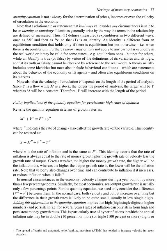
Heritage of monetary economics 37
quantity equation is not a theory for the determination of prices, incomes or even the velocityof circulation in the economy.
Note that a relationship or statement that is always valid under any circumstances is said tobe an identity or tautology. Identities generally arise by the way the terms in the relationshipare defined or measured. Thus, (1) defines (measured) expenditures in two different ways,once as MV and then as Py, so that (1) is an identity. An identity is different from anequilibrium condition that holds only if there is equilibrium but not otherwise – i.e. whenthere is disequilibrium. Further, a theory may or may not apply to any particular economy inthe real world or it may be valid for some states – e.g. equilibrium ones – but not for others,while an identity is true (or false) by virtue of the definitions of its variables and its logic,so that its truth or falsity cannot be checked by reference to the real world. A theory usuallyincludes some identities but must also include behavioral conditions – which are statementsabout the behavior of the economy or its agents – and often also equilibrium conditions onits markets.
Note also that the velocity of circulation V depends on the length of the period of analysis.Since Y is a flow while M is a stock, the longer the period of analysis, the larger will be Ywhereas M will be a constant. Therefore, V will increase with the length of the period.
Policy implications of the quantity equation for persistently high rates of inflation
Rewrite the quantity equation in terms of growth rates as:
M ′′ + V ′′ ≡ P′′ + y′′
where ′′ indicates the rate of change (also called the growth rate) of the variable. This identitycan be restated as:
π ≡ M ′′ + V ′′ − Y ′′
where π is the rate of inflation and is the same as P′′. This identity asserts that the rate ofinflation is always equal to the rate of money growth plus the growth rate of velocity less thegrowth rate of output. Ceteris paribus, the higher the money growth rate, the higher will bethe inflation rate, whereas the higher the output growth rate is, the lower will be the inflationrate. Note that velocity also changes over time and can contribute to inflation if it increases,or reduce inflation when it falls.4
In normal circumstances in the economy, velocity changes during a year but not by morethan a few percentage points. Similarly, for most economies, real output growth rate is usuallyonly a few percentage points. For the quantity equation, we need only consider the difference(V ′′ − y′′) between them. In the normal case, both velocity and output increase over time butthe difference in their growth rates is likely to be quite small, usually in low single digits.Adding this information to the quantity equation implies that high (high single digits or highernumbers) and persistent (i.e. for several years) rates of inflation can only stem from high andpersistent money growth rates. This is particularly true of hyperinflations in which the annualinflation rate may be in double (10 percent or more) or triple (100 percent or more) digits or
4 The spread of banks and automatic teller/banking machines (ATMs) has tended to increase velocity in recentdecades.
38 Introduction and heritage
even higher. Empirically, even at low inflation rates, the correlation between money supplygrowth and inflation rates over long periods is close to unity.
To reiterate, the source of inflation over long periods is usually money supply growth andthe source of persistently high inflation over even short periods is high and persistent moneygrowth rates. Therefore, if the monetary authorities wish to drastically reduce inflation ratesto low levels, they must pursue a policy that achieves an appropriate reduction in moneysupply growth.
2.1.1 Some variants of the quantity equation
There are several major variants of the quantity equation. One set of variants focuses attentionon the goods traded or the transactions in which they are traded, so that they modify theright-hand side of (1). The second set of variants imposes disaggregation on the mediaof payments (e.g. into currency and demand deposits) or changes the monetary aggregate,thereby modifying the left side of (1). We present some forms of each of these variants. Thefirst set of these variants is given by (i) and (ii) below. The second set is given by (iii).
(i) Commodities approach to the quantity equation
One way of measuring expenditures is as the multiple of the amount y of commodities sold inthe economy in the current period times their average price level P. Therefore, the quantityequation can be written as:
M · VMy ≡ Py · y (2)
where:VMy = income-velocity of circulation of money balances M in the financing of the
commodities in y over the designated periodPy = average price (price level) of currently produced commodities in the
economyy = real aggregate output/income in the economy.
(2) is often also stated as:
M · VMy ≡ Y (3)
(3) yields velocity VMy as equaling the ratio Y /M .
(ii) Transactions approach to the quantity equation
If the focus of the analysis is intended to be the number of transactions in the economy ratherthan on the quantity of goods, expenditures can be viewed as the number of transactions Tof all goods, whether currently produced or not, in the economy times the average price PT
paid per transaction. The concept of velocity relevant here would be the rate of turnoverper period of money balances in financing all such transactions. The quantity equation thenbecomes:
M · VMT ≡ PT · T (4)
Heritage of monetary economics 39
where:VMT = transactions-velocity of circulation per period of money balances M in
financing transactions TPT = average price of transactionsT = number of transactions during the period.
To illustrate the differences between y and T and between Py and PT , assume that weare dealing with a single transaction involving the purchase of ten shirts at a price of $10each. The total cost of the transaction is $100. Here, the quantity y of goods is 10 and theiraverage price Py is $10, while the number of transactions T is one and their average pricePT is $100.
(iii) Quantity equation in terms of the monetary base
The monetary base5 consists of the currency in the hands of the public (households andfirms), the currency held by the financial intermediaries and the deposits of the latter withthe central bank. Since the central bank has better control over the monetary base, whichit can manipulate through open market operations, than over M1 or M2, it is sometimesuseful to focus on the velocity of circulation VM0,y of the monetary base. This velocitydepends not only upon the behavior of the non-banking public but also upon the behaviorof firms and financial intermediaries. The quantity equation in terms of the monetarybase is:
M0 · VM0,y ≡ Py · y (5)
where:M0 = quantity of the monetary baseVM0,y = income-velocity of circulation per period of the monetary base.
The quantity equation is thus a versatile tool. Note that all versions of it are identities. Theform in which it is stated should depend upon the analysis that is to be performed. Examplesof such interaction between the intended use and the actual variant of the quantity equationemployed occur often in monetary economics.
2.2 Quantity theory
The quantity theory had a rich and varied tradition, going as far back as the eighteenthcentury. It is the proposition that in long-run equilibrium, a change in the money supplyin the economy causes a proportionate change in the price level, though not necessarily indisequilibrium.
The quantity theory was dominant in its field through the nineteenth century, though moreas an approach than a rigorous theory, varying considerably among writers and periods.Two versions of the form that it had achieved by the beginning of the twentieth century arepresented below from the works of Irving Fisher and A.C. Pigou. A third version, radicallydifferent from those of these writers, is presented later from the writings of Knut Wicksell.
5 The monetary base is also sometimes called the reserve base or high-powered money.

40 Introduction and heritage
2.2.1 Transactions approach to the quantity theory
Irving Fisher, in his book The Purchasing Power of Money (1911), sought to provide arigorous basis for the quantity theory by approaching it from the quantity equation. Herecognized the latter as an identity and added assumptions to it to transform it into a theoryfor the determination of prices. A considerable part of his argument was concerned withproviding a clear and relevant exposition of the quantity equation, and one of his versions ofthis equation is presented below.
Fisher distinguished between currency and the public’s demand deposits in banks. Thisdistinction was relevant to the economy when he wrote, since currency was commonly used inpayments whereas payments by check were much less common. Setting aside this distinctionfor the modern economy, we use M1 as the relevant money variable. Fisher also stated hisversion of the quantity theory in terms of the number of transactions, rather than in terms of thequantity of commodities purchased.6 However, as a result of Keynes’s emphasis on nationalincome/output rather than total transactions, while data on national income/output came tobe gathered and made commonly available, the data on the number of transactions was notgathered and has not become available in the public domain. The following, therefore, adaptsFisher’s treatment of the quantity equation and theory and couches it in terms of the amountof the commodities purchased rather than in terms of transactions. This adapted version ofthe quantity equation has the form:
MV ≡ Py (6)
To transform the quantity equation into the quantity theory, Fisher put forth twopropositions about economic behavior. These are:
(i) The velocities of circulation of “money” (currency) and deposits depend … ontechnical conditions and bear no discoverable relation to the quantity of money incirculation. Velocity of circulation is the average rate of “turnover” and depends oncountless individual rates of turnover. These … depend on individual habits. … Theaverage rate of turnover … will depend on density of population, commercial customs,rapidity of transport, and other technical conditions, but not on the quantity of moneyand deposits nor on the price level.(ii) (except during transition periods) the volume of trade, like the velocity of circulationof money, is independent of the quantity of money. An inflation of the currency cannotincrease the product of farms and factories, nor the speed of freight trains or ships. Thestream of business depends on natural resources and technical conditions, not on thequantity of money. The whole machinery of production, transportation and sale is amatter of physical capacities and technique, none of which depend on the quantity ofmoney.
(Fisher, 1911).
6 Fisher’s version of the quantity equation is CVC + DVD ≡ PT T , where C is currency and VC is its velocity, whileD is demand deposits and VD is its velocity. Total expenditures equal (CVC +DVD). Fisher maintained “that bankreserves are kept in a more or less definite ratio to bank deposits” and “that individuals, firms and corporationsmaintain more or less definite relations between their money (currency) and deposit balances.” Hence, C and Dwill always change in proportion. The alternative way of measuring expenditures in Fisher’s transactions approachwould be as PT ·T , where PT is the average price of transactions and T is the aggregate number of all transactionsagainst commodities.

Heritage of monetary economics 41
Therefore, Fisher’s conclusion was that:
while the equation of exchange is, if we choose, a mere “truism” based on the equivalence,in all purchases, of the money … expended, on the one hand, and what they buy on theother, yet in view of supplementary knowledge … as to the non-relation of [velocity tomoney and prices], this equation is the means of demonstrating the fact that normallythe prices vary directly as M, that is, demonstrating the quantity theory.
(Fisher, 1911, italics and the clause in brackets added).7
Fisher was certainly right in specifying that the transformation from his version ofthe quantity equation to the quantity theory requires that, when the monetary authoritiesincrease the amount of money, the velocity of circulation and the quantities of goods remainunchanged. These assertions, as well as (i) and (ii) above, are economic ones, resting onassumptions about human behavior, and may or may not be valid. In symbols and in the aboveupdated mode of statement of the quantity equation, these assertions become: ∂y/∂M = 0and ∂V/∂M = 0. These imply that, following an increase in the money supply, prices willrise in proportion to the increase in the money supply. That is, the elasticity of the price levelwith respect to the money supply will be unity.8
Fisher pointed out that the above assertions did not necessarily apply during “transition”(which can be interpreted as “disequilibrium”) periods, so that his assertions applied to acomparison of the equilibrium states prior to and after a one-time increase in the moneysupply. Fisher based these assertions on the then dominant theories of output and other realvariables (including velocity), for which the traditional classical approach and Walrasianmodel imply the independence of real variables from the monetary ones, which are M and P,in equilibrium.
On assumption (ii) of Fisher, the dominant theory – which was part of Fisher’s own views ofthe economy – of the early twentieth century on output and employment in the economy wasthe Walrasian one, which treated each market separately and used microeconomic analysis.9
This analysis implied that the labor market would clear in equilibrium and there would be fullemployment. Output would tend to stay at the full-employment level, except in the transientdisequilibrium stages. Further, this full-employment output was independent of the moneysupply and prices. Therefore, Fisher’s assertion that changes in the money supply wouldnot affect the equilibrium output of goods was consistent with the real economic theory ofthe time and was, in effect, based on the latter. This assertion was to be later challengedby Keynes and the Keynesians for demand-deficient economies, reaffirmed by the modernclassical economists in the 1980s and 1990s and denied by the new Keynesians in the lasttwo decades.10 Further, note Fisher’s qualification “except during transition periods” to thequantity theory proposition. Interpreting this as a reference to the disequilibrium induced byan exogenous change in the money supply, the real-time of this transition (from one long-run
7 The symbols have been changed and italicized in the above quotation as well as in following ones.8 To derive this from Fisher’s arguments, take the derivative, with respect to M , of the quantity equation MV ≡ Py,
where the symbol Q for real output has been replaced by y. This yields: V + M · ∂V /∂M = y · ∂P/∂M +P · ∂y/∂M . Fisher’s argument is that, in equilibrium, ∂V /∂M = 0 and ∂y/∂M = 0. Hence, in equilibrium,(M/P) · (∂P/∂M ) = 1, which is the quantity theory proposition.
9 See Chapter 1.10 See Chapters 14 to 17 for more information on these schools.
42 Introduction and heritage
equilibrium state to the one following a change in the money supply) becomes a very relevantquestion for the pursuit, or not, of monetary policy.
Fisher’s assumption (i) on the independence of velocities from changes in the moneysupply is also questionable. The velocity of circulation of money is not directly related tothe behavior of firms and households and, if one thinks solely in terms of velocity, Fisher’ssimplistic argument on this point seems reasonable. However, since velocity is a ratio ofexpenditures to money holdings, Fisher’s assertion becomes more easily subject to doubt ifthe determinants of velocity are approached from the determinants of expenditures and thedemand for money, as Keynesians do, and if the economy is not continuously in generalequilibrium at full employment. These determinants include interest rates and output, sothat changes in interest rates and in output can change both the demand for money and itsvelocity.
However, velocity is a real variable since it can be defined as equal to real incomedivided by the real money stock in the economy. Modern classical economists focus onvelocity as a real variable, as Fisher had done, and, along with other real variables, takeit to be independent of money supply and the price level in the long-run equilibriumstate of the economy. Hence, modern classical economists agree with both of Fisher’sassumptions for the general equilibrium – that is, with all markets clearing – state ofthe economy. Modern classical economists, therefore, with a model implying continuousfull employment, still maintain Fisher’s quantity theory assertion that an increase in themoney supply will cause a proportionate increase in the price level, with velocity remainingunchanged.
Keynesians question the empirical usefulness of the assumption of continuous long-rungeneral equilibrium (yielding full employment) since they maintain that continuous fullemployment does not normally exist in the economy. They also assert the dependence ofmoney demand on the interest rate and the dependence of the interest rate on liquiditypreference and the money supply. Hence, to the Keynesians, neither velocity nor outputis independent of the money supply. Therefore, Keynesians reject the validity of the quantitytheory both in terms of comparison across equilibrium states and in disequilibrium.
Determinants of velocity: constancy versus the stability of the velocity function
Equilibrium in the money market means that money demand equals money supply. Therefore,in this equilibrium, velocity can be redefined as the nominal income divided by moneydemand. As explained in subsequent sections of this chapter, money demand dependsupon many variables, of which the most important are national income and interest rates.As income rises, economies of scale in money holdings mean that money demand doesnot rise as fast, so that velocity increases. The interest rate is the cost of holding moneyrather than interest-paying financial assets, so that money demand falls as interest rates rise,which increases velocity. Therefore, velocity rises as income rises and also rises as interestrates rise.
Financial innovations in recent decades have created a variety of substitutes for M1 and M2,which have reduced their demand. Further, telephone and electronic banking have reducedthe need to hold large precautionary balances against unexpected needs for expenditures.This trend has been reinforced by the fall in brokerages costs of various types in switchingbetween money and other financial assets, so that individuals can manage their expenditureswith smaller money balances while holding larger amounts of interest-paying financial assets.These developments have reduced the demand for M1 and M2, so their velocity has risen

Heritage of monetary economics 43
considerably in recent decades. To illustrate, while the velocity of M1 in the USA was about6.3 in 1991, it rose to about 8.8 in 2000.
Table 2.1 shows that the velocity of circulation, which equals nominal national incomedivided by the money supply, in Canada, UK and USA is not a constant. In fact, it varieseven over periods as short as a day or month.
Fisher did not assume the constancy of velocity. His assumption was the independence ofvelocity – a real variable – from that of changes in the money supply and the price level inthe general equilibrium states of the economy. From an empirical perspective, velocity is nota constant in either the short term or the long term in actual economies. It is continuouslychanging in the economy. Some estimates of the average annual change in velocity for theUSA lie at about 3 percent to 4 percent.
To conclude, Fisher did not assume velocity to be a constant, nor is it constant in the realeconomy. Economic theory takes it to be an economic variable, determined in the economyby other economic variables. As its determinants change, velocity changes. The determinantsof velocity are discussed in greater detail later in this chapter.
Table 2.1 Changes in the velocity of money
Velocity of M1 and M211 for USA (US$ billions)
Y12 M1 M2 V1 (Y/M1) V2 (Y/M2)
1991 5803.075 916.0 3472.7 6.34 1.671995 7397.650 1150.7 3680.0 6.43 2.012000 9816.975 1112.3 4962.2 8.83 1.98
Velocity of M1 and M2+ for Canada (C$ billions)
Y M1 M2+ V1(Y/M1) V2 (Y/M2+)
1991 679.921 45.622 534.989 14.90 1.271995 810.426 62.674 618.447 12.93 1.312000 1076.577 114.91913 713.503 9.37 1.51
Velocity of M2 and M4 for UK (British pounds billions)
Y M2 M4 V2 (Y/M2) V4 (Y/M4)
1991 558.160 278.3 502.1 2.01 1.111995 719.747 437.0 622.6 1.65 1.162000 953.227 600.3 885.0 1.59 1.08
11 The data on M1, M2, M2+ and M4 in Table 2.1 are taken from Statistics on Payment Systems in the Group ofTen Countries, published by the Bank for International Settlements, various years.
12 The data on nominal GDP (Y in Table 2.1) are taken from the World Economic Outlook Database of theInternational Monetary Fund, September, 2006.
13 This figure is taken from Weekly Financial Statistics of the Bank of Canada, March 2, 2001.

44 Introduction and heritage
The Fisher equation on interest rates: distinction between nominal and realinterest rates
Another of Fisher’s contributions on monetary theory was his distinction between thenominal and real interest rates. This is embodied in what has been designated the Fisherequation.
The rate of interest that is charged on loans in the market is the market or nominal rateof interest. This has been designated by the symbol R. If the rational lender expects a rateof inflation πe, he has to consider the real interest rate r that he would receive on his loan.However, financial markets usually determine the nominal interest rate R. In perfect capitalmarkets, the ex ante relationship14 between the expected real interest rate re and the nominalinterest rate R is specified by
(1 + re) = (1 + R)/ (1 +πe) (7)
where πe is the expected inflation rate. If there exist both real bonds (i.e. promising a realrate of return r per period) and nominal bonds (i.e. promising a nominal rate of return R perperiod), the relationship between them in perfect markets would be:
(1 + R) = (1 + r) (1 +πe) (8)
At low values of re and πe, reπe → 0, so that (7) is often simplified to:
re = R −πe (9)
This states that the real yield that the investor expects to receive equals the nominal rateminus the expected loss of the purchasing power of money balances through inflation. (8) iscorrespondingly simplified to R = r +πe. (8) and (9) are known as the Fisher equation.
Note that the real value of the rate of return that the holder of a nominal bond wouldactually (i.e. ex post) receive from his loan is the actual real rate of interest (ra), which iscorrespondingly given by:
ra = R −π (9′)
In these equations, the definitions of the symbols are:R = nominal rate of interestra = actual (ex post) real rate of interest on nominal bondsr = real rate of interestre = expected real rate of returnπ = actual rate of inflationπe = expected rate of inflation.
14 One explanation for the Fisher equation is as follows. An investor investing one dollar in a “nominal bond”(i.e. paying a nominal rate of interest R) would receive $(1 + R) at the end of the period. If he were to buya “real bond” (i.e. paying a real interest rate r), he would receive (1 + r) in real terms (i.e. in commodities)at the end of the period. Given the expectations on inflation held at the beginning of the current period, theexpected nominal value at the end of the period of this real amount equals $(1+ r)(1+π e). The investor wouldbe indifferent between the nominal and the real bonds if the nominal return from both bonds were equal, i.e.(1+R) = (1+ r)(1+π e). With all investors behaving in this manner, perfect capital markets would ensure thisrelationship.

Heritage of monetary economics 45
If the actual rate of inflation were imperfectly anticipated, the actual yield ra on nominalbonds would differ from the expected one re and may or may not be positive. In fact,negative real interest rates are often observed during years of accelerating inflation, suchas in the 1970s, when the real yield on nominal bonds was often, and often persistently,negative.15
Fisher’s direct transmission mechanism
For the transmission mechanism from exogenous money supply changes to the endogenouschanges in aggregate demand and prices, Fisher argued that an increase in the money supplyleads its holders to increase their expenditures on commodities. Fisher’s version of thisdisequilibrium chain of causation from changes in the money supply to changes in the nominalvalue of aggregate expenditures is given in the following quotation. Fisher starts by assumingthat an individual’s money holdings are doubled, and continues as:
Prices being unchanged, he now has double the amount of money and deposits, whichhis convenience had taught him to keep on hand. He will then try to get rid of the surplusmoney and deposits by buying goods. But as somebody else must be found to take themoney off his hands, its mere transfer will not diminish the amount in the community.It will simply increase somebody else’s surplus.… Everybody will want to exchangethis relatively useless extra money for goods, and the desire so to do must surely driveup the price of goods. [This process will continue until prices double and equilibrium isrestored at the initial levels of output and velocity.]
(Fisher, 1911, italics added).
Fisher’s mechanism, by which changes in the money supply induce changes in aggregateexpenditures, has come to be known as the direct transmission mechanism of monetary policy,as compared with the indirect transmission mechanism, which relies upon the changes in themoney supply inducing changes in interest rates, which in turn induce changes in investment,which then cause changes in aggregate expenditures. The latter mechanism was incorporatedin the 1930s into the Keynesian and neoclassical macroeconomic models, but the formerwas revived by Milton Friedman and the 1970s monetarist models. The modern classicalmodels generally ignore the direct transmission mechanism and, as with the Keynesianmodels, incorporate the indirect transmission mechanism. However, the direct transmissionmechanism continues to be relevant to the poor whose expenditures are close to their incomes,and especially in economies in which the increase in the money supply is used to financefiscal deficits and initially ends up in the hands of people whose usual use of extra funds isto buy commodities.
2.2.2 Cash balances (Cambridge) approach to the quantity theory
Another popular approach to the quantity theory examined the determination of prices fromthe perspective of the demand and supply of money. Some of the best known exponents of
15 However, under the rational expectations hypothesis, the error in expectations would be only random anduncorrelated with information available at the time the expectations are formed, which implies that the real ratescould not be persistently negative.
46 Introduction and heritage
this approach were at Cambridge University in England and included, among others, AlfredMarshall, A.C. Pigou and the early writings (that is, pre-1936) of John Maynard Keynes.The following exposition of this approach follows that of Pigou in his article, The Value ofMoney (1917).
Pigou, like Fisher, defined currency or legal tender as money but was, in general, concernedwith what he called “the titles to legal tender.” He defined these titles as including currencyand demand deposits in banks, which correspond to the modern concept of M1. He arguedthat a person held currency and demand deposits:
to enable him to effect the ordinary transactions of life without trouble, and to securehim against unexpected demands due to a sudden need, or to a rise in the price ofsomething that he cannot easily dispense with. For these two objects, the provision ofconvenience and the provision of security, people in general elect to hold currency anddemand deposits.
(Pigou, 1917, italics added).
The actual demand for currency and demand deposits is:
determined by the proportion of his resources that the average man chooses to keep inthat form. This proportion depends upon the convenience obtained and the risk avoidedthrough the possession of such titles, by the loss of real income involved through theprovision to this use of resources that might have been devoted to the production of futurecommodities, and by the satisfaction that might be obtained by consuming resourcesimmediately and not investing at all.
(Pigou, 1917).
Pigou thus claimed that the individual is not directly concerned with the demand formoney but with its relation to his total resources. These resources can be interpretedas wealth in stock terms or as income/expenditures in flow terms. We will use thelatter, so that income will be the proxy for Pigou’s “resources.” Further, accordingto Pigou, this ratio of money demand to resources is a function of its services, theinternal rate of return on investments and of the marginal satisfaction foregone fromless consumption. Representing the internal rate of (real) return on investment as r andassuming it to be an approximate measure, in equilibrium, of the satisfaction foregone by notconsuming, the ratio of money balances demanded (M d) to total nominal expenditures (Y )is given by:
M d/Y = k(r) k ′(r) < 0 (10)
where k is a functional symbol. M d/Y decreases with r, or, in Pigou’s words, “the variable kwill be larger the less attractive is the production use and the more attractive is the rivalmoney use of resources.” Hence, ∂k/∂r < 0. Therefore, the demand for money balances,M d, is:
M d = k(r)Y (11)

Heritage of monetary economics 47
Determination of the price level in the cash balance approach
Assuming a given money supply M , equilibrium in the money market with (11) requires that:
M = k(r)Y (12)
Writing Py for Y , with P as the price level and y as the real amount of goods,
M = k(r) Py (13)
Assuming that output y is at its full employment level yf in equilibrium, y = yf , so that(11) becomes:
M = k(r) Pyf
where ∂yf/∂P = 0 and ∂yf/∂M = 0. Further, Pigou assumed16 that the equilibrium rate ofreturn (r∗) was determined by the marginal productivity of capital (MPK), which was taken tobe independent of the money supply and the price level, so that ∂r∗/∂P = 0 and ∂r∗/∂M = 0.Therefore, in equilibrium,
M = k(r∗) Pyf (14)
so that, in equilibrium,
P = M/[
k(r∗) · yf
](15)
which implies that:
∂P/∂M = 1/[
k(r∗) · yf
]and
EP·M = (M/P) · (∂P/∂M ) = 1
where EP·M . is the elasticity of P with respect to M . Since this elasticity equals unity, theprice level will, in comparative static equilibria, vary proportionately with the money supply.Therefore, (14) establishes Pigou’s version of the quantity theory proposition.
The cash balance approach starts its statement of the quantity theory as a theory of demand,supply and equilibrium in the money market and then proceeds to place it in a long-run generalequilibrium approach to the economy. From a rigorous standpoint, it does not become a theoryof the price level until the complete model – which includes the determination of output andinterest rates – is specified. On the latter variables, Pigou and his colleagues in the quantitytheory tradition had in mind the then generally accepted traditional classical ideas on thedetermination of output and interest rates. As stated in Chapter 1, these ideas implied the
16 Pigou implicitly did so in The Value of Money. This was consistent with his ideas on the determination of theequilibrium rate of return in the economy by the marginal productivity of capital.

48 Introduction and heritage
independence of the long-run equilibrium values of both these variables from the demand andsupply for money and turned the money market equilibrium equation (11) into a statementof the quantity theory. The essential deficiency in Pigou and the cash balance approachlay not so much in their specification of money demand relevant to the time in which theywere writing, but in that of the existing (traditional classical) macroeconomic analysis whichfailed to specify the determination of aggregate demand and its impact on output in short-runequilibrium, as well as in disequilibrium. This deficiency was the major point of attack byKeynes on the quantity theory and the traditional classical approach generally.
Velocity in the cash balance approach
On the velocity of circulation V in Pigou’s analysis, we have from (11) that:
V = Y /M
= 1/ [k(r)] (16)
In (13), since velocity depends upon the rate of interest, it is not a constant in the contextof Pigou’s money market analysis. However, given the independence of the equilibriumrate of interest and the marginal productivity of capital from the supply of money, theequilibrium level of velocity equals [1/k(r*)], which is independent of the supply of money.This independence of velocity with respect to the money supply does not mean its constancyover time, since velocity could still depend upon other variables, such as banking practicesand payment habits, and these often change over time. Further, the independence of velocityfrom the money supply was asserted only for equilibrium but not for disequilibrium. However,Pigou and other economists in the Cambridge school often fell into the habit of treating k as aconstant even though it was a functional symbol with k ′(r) < 0, so that velocity also becamea constant both in and out of equilibrium.
Legacy of the cash balance approach for the analysis of the demand for money
Further developments in monetary theory during the twentieth century built on two aspectsof the nineteenth and early twentieth century monetary theory. These were as follows: (i)The cash balance approach started its presentation of the quantity theory by analyzing thedemand for money and equilibrium in the money market. This idea was later taken up byMilton Friedman (whose contribution on this topic is presented later in this chapter) toidentify and confine the quantity theory to the analyses of the demand for money and themoney market; (ii) the cash balance approach had analyzed the demand for money in termsof its characteristics or functions, which were:
1 The provision of convenience in transactions.2 The provision of security against unexpected demands due to a sudden need or to a rise
in the prices.
The former was related to the demand for the medium of exchange function of money andthe latter to its store of value function. These reasons for holding money were restated byKeynes in 1936 into the transactions motive and the precautionary motive. Keynes added tothese the speculative motive.

Heritage of monetary economics 49
2.3 Wicksell’s pure credit economy
Knut Wicksell was a Swedish monetary economist writing within the classical tradition inthe last decades of the nineteenth and the first quarter of the twentieth century and consideredhimself to be an exponent of the quantity theory. His treatment of the quantity theory wasvery distinctive and quite different from the English and American traditions of the time, asrepresented in the works of Fisher, Pigou and Keynes during his classical period prior to 1930.Further, elements of Wicksell’s analysis led to the formulation of modern macroeconomicanalysis. His ideas have assumed even greater importance in the past two decades since severalcentral banks in developed economies have adopted the use of the interest rate as their primarymonetary policy instrument, so that the appropriate analysis has to take the interest rate ratherthan the money supply as being exogenously set. The money supply becomes endogenous inthis context. These assumptions are essentially similar to those made by Wicksell. The newKeynesian analysis embodies these assumptions, so that it is sometimes referred to as theneoWicksellian analysis.
Wicksell sought to defend the quantity theory as the appropriate theory for the determina-tion of prices against its alternative, the full cost pricing theory. The latter argued that eachfirm sets the prices of its products on the basis of its cost of production, including a marginfor profit, with the aggregate price level being merely the average of the individual pricesset by firms. The amount of the money supply in the economy adjusts to accommodate thisprice level and is therefore determined by the price level, rather than determining it. Wicksellconsidered this full cost pricing theory as erroneous and argued that such pricing by firmsdetermined the relative prices of commodities, rather than the price level. In his analysis, thelatter was determined by the quantity of money in the economy relative to national outputsince commodities exchange against money and not against each other.
In his reformulation of the quantity theory, Wicksell (1907) sought to shift the focus ofattention to the transmission mechanism relating changes in the money supply to changesin the price level. He specified this mechanism for economies using either metallic or fiatmoney and for a pure credit economy. The latter analysis is the more distinctive one andillustrates Wicksell’s transmission mechanism more clearly. It is also the one likely to bemore relevant to the future evolution of our present day economies and, therefore, is the onepresented below.
In modern macroeconomic terminology, Wicksell’s analysis of the pure credit economyis essentially short run since his analysis assumes a fixed capital stock, technology andlabor force in the production of commodities. This focus on the short run contrasts withFisher’s and Pigou’s reliance on the long-run determination of output in order to establishtheir versions of the quantity theory. Further, Wicksell assumes that the economy is a purecredit one in the sense that the public does not hold currency and all transactions are paidby checks drawn on checking accounts in banks, which do not hold any reserves againsttheir demand deposits. Since the banks do not hold reserves and any loans made by themare re-deposited by the borrowers or their payees in the banks, the banks can lend anyamount that they desire without risking insolvency. Further, banks are assumed to be willingto lend the amount that the firms wish to borrow at the specified market rate of interestset by the banks. Wicksell calls the nominal rate of interest at which the banks lend tothe public the money or market rate of interest. The banks accommodate the demand forloans at this interest rate, which is set by them. Under these assumptions, the amount ofmoney supply in the economy is precisely equal to the amount of credit extended by thebanks, since these loans are wholly deposited in the banks. Hence, changes in the money

50 Introduction and heritage
supply occur only when the demand for loans changes in response to an exogenous shiftin the interest rate charged by banks. Note that, in Wicksell’s pure credit economy, theeconomy’s interest rate is set exogenously by the banks, while the money supply dependson this interest rate and the public’s demand for loans. Therefore, it is endogenous to theeconomy.
A critical element of Wicksell’s (1907) theory is the emphasis on saving and investmentin the economy. Funds for (new) investment come from saving plus changes in the amountof credit provided by banks. The rate of interest which equates saving and investment waslabeled by Wicksell the normal rate of interest. Since Wicksell’s pure credit economy was aclosed one and there was no government sector, the equality of saving and investment meansthat the normal rate of interest is the macroeconomic equilibrium rate. Further, if the marketinterest rate equals the normal rate, there will be no change in the credit extended by banksand, therefore, no change in the money supply. For a stable amount of credit and moneysupply in the economy, the price level will remain unaltered. To conclude, at the market rateof interest equal to the normal one, there is equilibrium in the commodity market, Further,with stable output and money supply, the normal rate of interest will be accompanied by astable price level.
Firms borrow to finance additions to their physical capital. The marginal productivity ofcapital specifies the internal rate of return to the firm’s investments and was referred to byWicksell as the natural rate of interest. The firm’s production function has diminishingmarginal productivity of capital, so that, with a constant labor force and unchangedtechnology, the natural rate of interest decreases as capital increases in the economy.
To see the mechanics of this model, start from an initial position of equilibrium in theeconomy, with a stable money supply and prices, and with the equality of the market/loanand natural rates of interest at the normal/equilibrium rate of interest. Now, suppose thatwhile the market rate of interest is held constant by the banks, the marginal productivity ofcapital rises. This could occur because of technological change, discovery of new mines, afall in the real wage rate, etc. Firms can now increase their profits by increasing their capitalstock and production. To do so, they increase their investments in physical capital and financethese by increased borrowing from the banks. This causes the amount of credit and moneysupply in the economy to expand.
Wicksell appended to this analysis the disaggregation of production in the economybetween the capital goods industries and the consumer goods industries. As the demandfor investment in physical capital increases, factors of production are drawn into suchindustries from the consumer goods industries, so that the output of the latter falls. Atthe same time, the competition for labor and the other factors of production will drive upworkers’ incomes, leading to an increase in the demand for consumer goods, thereby pushingup prices. Consequently, the price level will rise, though with a lag behind money supplychanges. Analysis based on this disaggregation of production between the capital goodsindustries and the consumer goods industries is not a feature of most modern macroeconomicmodels.
Cumulative price increases (the inflationary process)
In the above process, initiated by a reduction by the banks of the market interest rate belowthe natural one or by an increase in the latter above the market rate, the price rise willcontinue as long as the market rate of interest is below the natural rate, since the firms willthen continue to finance further increases in investment through increased borrowing from

Heritage of monetary economics 51
the banks. This constitutes a process of cumulative price increases. These increases can onlycome to an end once the banks put an end to further increases in their loans or credit to firms.A closed pure credit economy does not provide a mechanism that will compel the banks todo this.
However, in an open economy where the banking system keeps gold reserves out of whichdeficits in the balance of payments have to be settled, gold outflows provide a limit to thecumulative price increases. In such a context, as prices continue to increase, foreign tradedeficits develop, the gold reserves of banks fall and the banks raise their loan rate of interestto the natural rate to stem the outflow of gold. This is especially so if the banks hold goldas part of their reserves and the public holds gold coins circulating as currency for sometransactions. In the latter case, as prices rise, the public’s demand for currency will alsoincrease and gold will flow out of the banks’ reserves to the public. Such losses of the goldreserves to the public and abroad forces banks to restrict their lending to the firms by raisingtheir loan rate to match the natural rate. This puts an end to the cumulative credit and moneysupply increases and therefore to the cumulative price increases.
This cumulative process can also be initiated by banks arbitrarily lowering the marketrate below the natural rate, with the resultant adjustments being similar to those specifiedabove for an exogenous increase in the natural rate. However, Wicksell viewed the bankersas being conservative enough not to change the market rate except in response to changesin their gold holdings or an exogenous change in the normal rate. Therefore, in Wicksell’sview, the cumulative price increase was usually a result of exogenous changes in the marginalproductivity of capital impinging on an economy whose credit structure responds with gradualand possibly oscillatory adjustments – for example, if the banks sometimes overdo theadjustment of the market rate.
Wicksell’s re-orientation of the quantity theory to modern macroeconomics
Wicksell’s treatment of the pure credit economy clearly re-oriented the quantity theory in thedirection of modern macroeconomic analysis. Several features of this analysis are relevantto modern macro and monetary economics. Among these is Wicksell’s focus on the short-run treatment of the commodity market in terms of the equilibrium between saving andinvestment, a focus that was later followed and intensified in the Keynesian approach, aswell as in the IS–LM modeling of short-run macroeconomics. While Wicksell claimed tobe a proponent of the quantity theory of money, he shifted its focus away from exclusiveattention on the monetary sector, for example, as in Pigou’s version of the quantity theory,to the saving-investment process. In doing so, he led the way to the formulation of currentmacroeconomics, with the treatment of the commodities market at its core. This was to appearlater as the IS relationship of modern macroeconomics.
Wicksell introduced into macroeconomics a fundamental aspect of the modern monetaryeconomies: loans are made in money, not in physical capital, so that the rate of interest onloans is conceptually different from the productivity of physical capital. Even if they areequal in equilibrium, they will usually not be equal in disequilibrium. These ideas led theway to the analysis of the impact that the financial institutions and especially the central bankcan have on the interest rates in the economy and on national income and employment.
Wicksell’s analysis of the pure credit economy also emphasized the role of interest ratesand financial institutions in the propagation of economic disturbances, since they control themarket interest rate, reduction in which can set off an expansion of investment, loans andthe money supply and lead to a cumulative increase in prices and nominal national income.
52 Introduction and heritage
Further, Wicksell assumed that the banking system sets the interest rate rather than themoney supply as the exogenous monetary constraint on economy. This assumption wasnot followed by the expositions of macroeconomic theory in either the classical or theKeynesian formulations until the end of the twentieth century, since they continued to take themoney supply as their exogenously determined monetary policy variable. Since the money-demand function proved to be unstable in most developed economies after the 1970s, therebyimplying the instability of the LM curve, many central banks now choose to use the interestrate as the monetary policy variable and set its level, while allowing the economy to determinethe money supply as an endogenous variable for the set interest rate. This practice came tobe reflected in the theories offered by the new Keynesian approach after the early 1990s.Wicksell was clearly the precursor of this type of analysis.
However, compared with the Keynesians, Wicksell, just like Fisher and Pigou, did not payparticular attention to the changes in the national output that might occur in the cumulativeprocess. While he discussed disequilibrium and transient changes in national output duringthis process, he was not able to shake off the classical notion that the economy will eventuallybe at full employment, so that his overall discussion was usually within the context of animplicitly unchanged equilibrium level of output. Given this background, Wicksell claimedthat increases in the money supply are accompanied sooner or later by proportionate priceincreases. Keynes’s General Theory (1936) was to question the implicit assumption of anunchanged level of output and to allow for changes in output and unemployment followinga change in aggregate demand. Merging this possibility into Wicksell’s cumulative processwould mean that his cumulative process would possess both output and price increases(decreases) whenever the market interest rate was below (above) the natural rate.
Hence, while Wicksell claimed nominal adherence to the traditional classical approachand the quantity theory, his theoretical macroeconomic analysis differed from theirs andwas quite modern in several respects. One, in terms of this theoretical analysis in termsof saving and investment, Wicksell was a precursor of the Keynesian and modern short-run macroeconomic analysis. Two, in terms of his assumption of a pure credit economy,he presaged current developments in the payments system. Three, his assumption that thefinancial system sets the interest rate rather than the money supply as exogenous, he was aprecursor of current central bank practices and the analysis of the new Keynesian models inthe last couple of decades.
However, Wicksell’s analysis did have at least several deficiencies relative to currentmonetary economics. One, although Wicksell did approach equilibrium through the normalinterest rate which equates saving and investment, he did not present a theory of aggregatedemand and also did not present the analysis of the impact of changes in it on outputand employment. These were to be later addressed by Keynes. Two, Wicksell did notdistinguish between real and nominal interest rates, which Fisher’s equation later clarified.Three, he did not pay much attention to the analysis of the demand for money, on whichKeynes made very significant contributions which provide the basis for its modern mode oftreatment.
2.4 Keynes’s contributions
Keynes’s contributions to macroeconomics
Keynes’s The General Theory (1936) represents a milestone in the development ofmacroeconomics and monetary thought. His contributions were so many and so substantial

Heritage of monetary economics 53
that they led to the development of the new field of macroeconomics, which had not existedin economic thought prior to The General Theory. These contributions also led to a new wayof looking at the performance of the economy and to an emphasis on departures from itslong-run equilibrium (full employment) and the establishment of the Keynesian paradigm(see Chapter 15) in macroeconomics.
Given the very many new contributions in this book, economists have debated asto which was the most important of these contributions.17 From a modern perspective,Keynes’s emphasis on aggregate demand as a major short-run determinant of aggregateoutput and employment seems to have had a lasting impact on economic theory and policy.Every presentation of macroeconomic theory now includes the determination of aggregatedemand and its relationship, embodied in the IS curve, to investment and fiscal policy.This contribution was based on the concept of the multiplier, which was unknown in thetraditional classical period. Keynes’s impact on monetary policy is reflected in central banks’manipulation of aggregate demand through either the use of the money supply or/and theinterest rate, in order to maintain inflation and output at their desired levels.
Again, in terms of the modern perspective, Keynes’s emphasis was on decisions onproduction and investment being made by firms on the basis of their expectations of futuredemand, and on consumption by households on the basis of their expected incomes. Thesedecisions are usually made under uncertainty, with imperfect information on the future.Following any shifts, the reactions by firms and households to changes in demand andincome prospects are often faster than by heterogeneous commodity and labor markets inadjusting prices and wages, so that the economy often produces more or less than the long-run equilibrium (full employment) output that efficient (i.e. instantly adjusting) marketswill ensure. The economy is, therefore, usually likely to end up with more or less than fullemployment. This provides the scope for the pursuit of monetary and fiscal economies tostabilize the economy. This scope is currently reflected in the espousal of Taylor-type rulesfor monetary policy.
Contrary to the assumptions of the quantity theory, The General Theory asserted theusual absence of full employment in the economy. This is clearly a factual issue, whichis undeniable in the context of the Great Depression of the 1930s and in many recessions.In the context of actual employment below the full-employment level, Keynes argued thatoutput and employment depended on the aggregate demand for commodities, which, inturn, depended on the money supply, so that money was not neutral. In the context ofthe lengthy post-war booms in the Western economies, the contribution of high and risingaggregate demand in pushing output and employment beyond their full-employment rates isalso generally recognized. The current manifestation of this recognition can be seen in thepursuit by central banks of Taylor-type rules, in which the output gap can be positive (withoutput above its full-employment level) or negative, with appropriate increases and decreasesin interest rates expected to reduce the output gap.
Keynes, in his earlier (pre-1936) writings, had proved to be an able and innovative exponentof the quantity theory in its Cambridge school version. He had also extensively exploredthe effects of changes in the money stock, though still mainly within the quantity theorytradition, in the two volumes of his book The Treatise on Money, published in 1930. Keynes’sapproach to the quantity theory in the Treatise, as in Wicksell’s writings, was in terms ofsaving and investment. In The General Theory, Keynes extended this saving-investment
17 Samuelson’s (1946) obituary article on Keynes provides very valuable insights into Keynes’s contributions.
54 Introduction and heritage
approach, while abandoning the quantity theory and the traditional classical approachgenerally.
This chapter mainly examines Keynes’s contributions on the demand for money inThe General Theory. As a prelude to these, remember that Pigou’s basic reasons forthe demand for money balances were the “objects” of the provision of convenienceand the provision of security. Keynes re-labeled “objects” as “motives” for holdingmoney balances and categorized them as the transactions, precautionary and speculativemotives. Of these, the transactions motive corresponded basically to the provision ofconvenience “object” of Pigou and the precautionary motive corresponded basically tothe provision of security “object” of Pigou. Keynes was more original with respect to hisspeculative motive and his analysis of the demand for money balances arising from thismotive.
2.4.1 Keynes’s transactions demand for money
Keynes defined the transactions motive as:
The transactions-motive, i.e. the need of cash for the current transaction of personal andbusiness exchanges.
(Keynes, 1936, Ch. 13, p. 170).
The transactions motive was further separated into an “income-motive” to bridge theinterval between the receipt of income and its disbursement by households, and a “business-motive” to bridge the interval between payments by firms and their receipts from the sale oftheir products (Keynes, 1936, Ch. 15, pp. 195–6). Keynes did not present a rigorous analysisof the transactions and precautionary motives but “assumed [them] to absorb a quantity ofcash which is not very sensitive to changes in the rate of interest as such … apart from itsreactions on the level of income” (Keynes, 1936, p. 171). This assumption of Keynes wasin fact somewhat more restrictive than that of Pigou where the demand for money, due tothe objects of the “provision of convenience” and the “provision of security,” was dependentupon the return on investments and the utility foregone in abstaining from consumption.Designating the joint transactions and precautionary demand for money balances as M tr andnominal income as Y , Keynes assumed that:
M tr = M tr (Y ) (17)
where M tr increases as Y increases.Now consider the ratio (Y /M tr), which is the velocity of circulation of transactions balances
alone in the preceding equation. Here, Keynes followed the simplistic pattern of Pigou’sreasoning in stating that
There is, of course, no reason for supposing that V (= Y /MT) is constant. Its value willdepend on the character of banking and industrial organization, on social habits, on thedistribution or income between different classes and on the effective cost of holding idlecash. Nevertheless, if we have a short period of time in view and can safely assume nomaterial change in any of these factors, we can treat V as nearly enough constant.
(Keynes, 1936, p. 201).

Heritage of monetary economics 55
This reasoning implies that Y /M tr is a constant k , independent of income and interest rates,so that Keynes’s transactions demand for money was:
M tr = kY (18)
The modern analysis of transactions demand did not follow Keynes’s simplistic assumptionon its constancy, but applies inventory models to it, which makes this demand a function ofthe interest rate. This analysis is presented in Chapter 4.
2.4.2 Keynes’s precautionary demand for money
Keynes’s second motive for holding money was the precautionary one, defined by him as
the desire for security as to the future cash equivalent of a certain proportion of totalresources.
(Keynes, 1936, Ch. 13, p. 170).
Another definition of this motive was given later in Chapter 15 of The General Theory as
To provide for contingencies requiring sudden expenditure and for unforeseen opportu-nities of advantageous purchases, and also to hold an asset of which the value is fixedin terms of money.
(Keynes, 1936, Ch. 15, p. 196).18
That is, the precautionary motive arises because of the uncertainty of future incomes, aswell as of consumption needs and purchases. These require holding money, an asset with acertain value, to provide for contingencies that suddenly impose payment in money. Thesecontingencies could come from a sudden loss of income due to the loss of one’s job, ora sudden increase in consumption expenditures, such as from becoming ill and requiringtreatment.
Under uncertainty, the individual will form subjective expectations on the amounts requiredfor his future payments and income receipts, and their dates, and will decide on the optimalamounts of his money balances and other assets in the light of these expectations. The furtherahead are the dates of anticipated expenditures and the greater is the yield from investments,the more likely is the individual to invest his temporarily spare funds in bonds and decreasehis money holdings. Conversely, an increase in the probability of requirement in the nearfuture will lead him to increase his money holdings and decrease his bond holdings.
Although Keynes provided the rationale for the precautionary motive for holding money,he did not present a theoretical derivation of the precautionary demand for money. Rather,he merged it with the transactions demand for money. However, subsequent developmentson money demand did come up with several models of the precautionary demand for moneyand its related buffer stock demand (see Chapter 6).
18 Keynes provided another definition of the precautionary motive on page 169 of Chapter 13. This definitiondiffers from that in the above quotation from Chapter 15. The modern interpretation of the precautionary motiveis as given in the text below the quotation.

56 Introduction and heritage
2.4.3 Keynes’s speculative money demand for an individual
Keynes’s third motive for holding money was:
3. The speculative-motive, i.e. the object of securing profit from knowing better than themarket what the future will bring forth.
(Keynes, 1936, Ch. 13, p. 170).
Keynes had earlier explained this motive as resulting:
from the existence of uncertainty as to the future of the rate of interest, provided thatthere is an organized market for dealing in debts. For different people will estimate theprospects differently and anyone who differs from the predominant opinion as expressedin market quotations may have a good reason for keeping liquid resources in order toprofit, if he is right … the individual who believes that future rates of interest will beabove the rates assumed by the market, has a reason for keeping liquid cash, whilstthe individual who differs from the market in the other direction will have a motive forborrowing money for short periods in order to purchase debts of longer term. The marketprice will be fixed, at the point at which the sales of the “bears” and the purchases of the“bulls” are balanced.
(Keynes, 1936, Ch. 13, pp. 169–70).
In this motive, the individual makes a choice between holding money, which does not payinterest, and bonds, which provide an uncertain return, on the basis of maximizing the returnto his portfolio. With a given amount to invest in bonds or hold in money balances, he isconcerned with the maturity value – equal to the capital invested plus accumulated interest –of his portfolio at the beginning of the next decision period. Assuming such a value to beuncertain, Keynes postulated a rather simple form of the expectations function: the individualanticipates a particular rate of interest to exist at the beginning of his next decision period,thereby implying a particular expected price, without dispersion,19 for each type of bond. Ifthese expected bond prices plus the accumulated interest are higher than the current prices,he expects a net gain from holding bonds, so that he will put all his funds in bonds rather thanin money which was assumed not to pay interest and therefore to have zero net gain. If heexpects a sufficiently lower price for bonds in the future than at present to yield a net loss20
from holding bonds, he will put all his funds into money balances since there is no loss fromholding these. Consequently, a particular individual will hold either bonds or money but notboth simultaneously.
Since individuals tend to differ in their views on the future of the rate of interest, somewould expect an increase in bond prices and are labeled as bulls in bond market parlance,choosing to increase their bond holdings, while others would expect a decrease in bond pricesand are labeled as bears, choosing to reduce their bond holdings. Any increase in bond priceswill exceed the expectations of some bulls – that is, convince them that bond prices have goneup too far and convert them into bears. A preponderance of bulls in the bond market pushesup the prices of the bonds and pushes down the rate of interest. This movement converts an
19 This simplification was subsequently abandoned in the 1950s by monetary economics in the application ofportfolio selection analysis to the speculative demand for money, presented in Chapter 5 below.
20 There will be a net loss if the capital loss is greater than the interest income from holding the bond.

Heritage of monetary economics 57
increasing number of bulls (who want to buy and hold bonds) into bears (who want to sellbonds and hold money), until an equilibrium price of bonds is reached where the demand forbonds just equals their supply. Therefore, the demand for speculative money balances – bybears – increases as the prices of bonds rise, or conversely, as the interest rate falls, so thatthe aggregate speculative demand for money is inversely related to the rate of interest.
Modern monetary and macroeconomic theory has abandoned this line of reasoning andhas instead opted for an analysis based on portfolio selection, so that a better name for themoney demand derived from portfolio selection analysis would be the “portfolio demand formoney.” This approach is presented in Chapter 5.
Tobin’s formalization of Keynes’s speculative money demand for an individual
Tobin’s (1958)21 formalization of Keynes’s speculative demand analysis has become a classicand is presented in the following.
As with Keynes’s analysis, Tobin assumes that there are only two assets, money and bonds,in which the individual can invest the amount of funds in his portfolio. Money is assumed tohave a known yield of zero and is therefore riskless in the sense of possessing a zero standarddeviation of yield. The bond is a consol, also known as a “perpetuity” in the United States,and has the characteristic that it does not have a redemption date, so that the issuer need neverredeem it but may continue to make the coupon payment on it indefinitely.
In perfect capital markets, the market price of a consol will equal its present discountedvalue. Therefore, the price pb of a consol which has a nominal coupon payment c per period,and is discounted at a market rate of interest x on loans, is given by:22
pb = c
1 + x+ c
(1 + x)2+ ·· ·
=c
( ∞∑t=1
1
(1 + x)t
)
=c
(1
x
)= c
x
Therefore, the consol’s value will equal its coupon rate (in perpetuity) divided by the marketrate. For a given coupon value, an increase in the market interest rate will reduce the consol’sprice and imply a capital loss. In the special case of a bond that has the same coupon rateas the market discount rate, c = x, so that its market value will equal unity, i.e. pb = 1.
21 Parts of the analysis of this article are presented later in Chapter 5 on the speculative demand for money.22 The proof uses the mathematical formula that, for x > 0,
∞∑t=1
1
(1 + x)t= 1
x
Many bonds have a finite redemption date, say n. For this, the relevant formula is
n∑t=1
Dt =n∑
t=0
Dt − 1 = 1 − Dn+1
1 − D− 1
where D = 1/(1 + x). Since x > 0, Dn+1 → 0 as t → ∞.
58 Introduction and heritage
Now assume that the market interest rate is $R per year and the consol is expected to pay acoupon $R per year in perpetuity. With a coupon of R in perpetuity, the above mathematicalformula implies that the consol’s present value at the market interest rate R would equal R/Rand be 1.
Assume for the following analysis that the coupon payment on the consol is set at R andits current price is one dollar. Further, assume that the individual expects the market rate ofreturn on consols to be Re for the future, with this expectation held with a probability of oneand independent of the current yield R. With R treated as the coupon payment and the rateof discount expected to be Re in perpetuity, the expected value of the consol next year willbe R/Re. Therefore, the expected capital gain or loss G on the consol will be:
G = R/Re − 1
The expected yield (R + G) from holding a consol costing $1 is the sum of its coupon Rand its capital gain G. This sum is given by:
R + G = R + R/Re − 1
If the yield (R + G) were greater than zero, the rational individual would buy only consols,since they would then have a yield greater than money, which was assumed above to havea zero yield.23 Conversely, if the yield on consols were negative, the individual would holdonly money since money would be the asset with the higher yield.
The switch from holding bonds to money occurs at R+G = 0. This condition can be usedto derive the critical level Rc of the current return R such that:
Rc = Rc/Re − 1 = 0
which implies that:
Rc − Re/[1 + Re]
For a given Re, if the current interest rate R is above Rc, (R + G) > 0 and only consolswill be bought; if it is below Rc, (R + G) < 0 and only money will be held. Therefore, inFigure 2.1, the individual’s demand for money is the discontinuous step function (AB, CW);above Rc, the rational individual’s whole portfolio W is held in consols and the demand formoney along AB is zero; below Rc, all of W is held in money balances and the demandfunction is CW.
2.4.4 Keynes’s overall speculative demand function
Keynes had argued that the bond market has a large number of investors who differ in theirexpectations such that the lower the rate of interest, the greater will be the number of investorswho expect it to rise, and vice versa. Therefore, at high rates of interest, more investors will
23 Risk does not enter this choice since the individual’s expectations are so firm that the subjective standarddeviation of expected yields is zero. Measuring risk by the standard deviation of expected yields, the zerostandard deviation means that the individual does not believe there to be any risk in holding consols.

Heritage of monetary economics 59
Msp
Rc,B
W
A
C
R
Figure 2.1
R
Msp
Msp
Figure 2.2
expect the rate to fall and few will hold money. At a somewhat lower rate of interest, asmaller number of the investors will expect the interest rate to fall and more of them willhold money. Hence, the aggregate demand for money will rise as the interest rate falls, andis shown as the continuous downward sloping curve M sp in Figure 2.2. Therefore, Keynes’sanalysis implies that the speculative demand for money depends inversely upon the rate ofinterest, so that the speculative demand function for money can be written as:
M sp = L (R) (19)
where:M sp = speculative demand for moneyR = market/nominal rate of interest.
Keynes called the function L(R) the degree of liquidity preference, with L standing forliquidity.
Note that in Keynes’s analysis, the individual allocates his financial wealth FW betweenmoney and bonds. Hence, in addition to the interest rate, financial wealth FW must be oneof the determinants of their demand. Therefore, (19) needs to be modified to:
M sp = L (R,FW )
60 Introduction and heritage
There also exists the possibility that the economy could substitute among money, bonds andcommodities as stores of value.24 The analysis allowing this possibility would need to broadenthe relevant wealth variable to total wealth and also make the speculative money demandfunction a function of both the return on bonds and that on commodities.25 This extension ofKeynes’s analysis leads to Friedman’s money demand function in the next section. For thetime being, we continue with (19) for Keynes’s specification of the speculative demand formoney, thereby simplifying it by ignoring wealth as a determinant of the speculative demandfor bonds.
2.4.5 Keynes’s overall demand for money
Keynes argued that:
Money held for each of the three purposes forms … a single pool, which the holder isunder no necessity to segregate into three watertight compartments; for they need notbe sharply divided even in his own mind, and the same sum can be held primarily forone purpose and secondarily for another. Thus we can – equally well, and, perhaps,better – consider the individual’s aggregate demand for money in given circumstancesas a single decision, though the composite result of a number of different motives.
(Keynes, 1936, p. 195; italics added).
Hence, the aggregate demand for money, M , depends positively upon the level of incomeY due to the transactions and precautionary motives and negatively upon the rate of interestR due to the speculative motive. In symbols,
M d = M tr + M sp = M (Y ,R)
However,
whilst the amount of cash which an individual decides to hold to satisfy the transactions-motive and the precautionary-motive is not entirely independent of what he is holdingto satisfy the speculative motive, it is a safe first approximation to regard the amountsof these two sets of cash-holdings as being largely independent of one another.
(Keynes, 1936, p. 199).
Hence, as an approximation, the demand function for money balances M d is given by:
M d =M tr + M sp
=kY + L (R) = kPy + L (R) (20)
where k > 0 and L(R) < 0.
24 In the context of Keynes’s analysis of bulls and bears, an expectation of inflation, with bond yields below theexpected inflation rate, would mean a flight from both money and money into commodities.
25 Further, the complete analysis will also have to examine the determinants of W. In particular, as the earlierdiscussion on consols illustrates, financial wealth will be a function of the interest rate R.

Heritage of monetary economics 61
2.4.6 Liquidity trap
Keynes argued that the speculative demand for money would become “absolute” (infinitelyelastic) at that rate of interest at which the bond market participants would prefer holdingmoney to bonds, so that they would be willing to sell rather than buy bonds at the existingbond prices. Following Keynes’s reasoning, the liquidity trap occurs at the rate of interestat which a generally unanimous opinion comes into being that the rate of interest willnot fall further but may rise. At this rate, there would be a general opinion that bondprices will not rise but could fall, thereby causing capital losses to bondholders, with theexisting rate of interest merely compensating for the risk of such a capital loss. In suchcircumstances, the public would be willing to sell all its bond holdings for money balancesat their existing prices, so that the monetary authorities could buy any amount of the bondsfrom the public and, conversely, increase the money holdings of the public by any amount,at the existing bond prices and rate of interest. Therefore, once the economy is in theliquidity trap, the monetary authorities cannot use increases in the money supply to lowerthe interest rate.
As against this analytical presentation of the liquidity trap, Keynes asserted that “whilstthis limiting case might become practically important in future, I know of no example of ithitherto” (Keynes, 1936, p. 207). Note that this assertion was made in the midst of the mostsevere depression in Western history; if the liquidity trap did not exist then, it can hardlyhave existed in more normal periods of economic activity. Hence, in Keynes’s view, whilethe liquidity trap is an intellectual curiosity for monetary economics, it is not of practicalrelevance. Consequently, contrary to some expositions or critiques of Keynesian economicsin earlier decades, Keynes did not build his macroeconomic model on the assumption of theliquidity trap.
Keynes’s statement on the empirical non-existence of the liquidity trap is strictly incorrectunder his own analysis of the speculative demand for money. In this analysis, the liquiditytrap will come into existence whenever the dominant opinion in the bond market is that themarket interest rates are going to rise, not decline. Such an opinion does quite frequently comeinto existence in the bond markets, so that the liquidity trap is not unknown in them. Further,such an opinion can exist at any level of the rate of interest and not merely at low or evensingle-digit rates. Furthermore, the liquidity trap will continue to exist until the dominantmarket opinion changes to envision possible decreases in the rate of interest.26 This wouldhappen once the interest rates have adjusted to the market opinion, so that the liquidity trapwould usually exist for short periods, which may not be long enough to affect investmentand the macroeconomy. Therefore, while liquidity traps may often come into existence in thenormal day-to-day functioning of bond markets, their existence for macroeconomics couldbe quite insignificant.
In contrast to Keynes’s reasoning, which emphasized the possibility of a capital gain orloss on holding bonds, for the existence of a liquidity trap, is the argument that nominalinterest rates close to zero do not compensate individuals for the hassle and inconvenienceof holding bonds when they could forgo these by holding money balances. This argument issupported by the analysis of the transactions demand for money presented in Chapter 4, whereit is shown that, at low enough interest rates relative to the brokerage costs of conversionbetween bonds and money, it is not profitable to hold bonds, so that only money will be
26 This, of course, is difficult to envision if the interest rate is already zero.

62 Introduction and heritage
held; thus, in this low enough range of interest rates, the interest elasticity of money demandwill be zero. In recent years, Japan is among the very few countries that have had short-terminterest rates close to zero. Some empirical studies do report that the interest elasticity ofmoney demand is much higher during Japan’s low interest rate period than in other periods(see, for example, Bae et al., 2006).
2.4.7 Keynes’s and the early Keynesians’ preference for fiscalversus monetary policy
Volatility of money demand
Keynes’s analysis of the speculative demand for money made it a function of the subjectiveexpectations of the bulls and bears in the bond and stock markets. Such expectations werequite volatile in the 1930s and can be quite volatile even nowadays, as one can observe inthe day-to-day volatility of the stock markets and the periodic “collapse” or sharp run-ups ofprices in them. Given this volatility, Keynes asserted that the speculative demand functionfor money was very volatile – that is, this function shifts often. Since Keynes believed thatthe speculative demand for money was a significant part of the overall demand for money, thelatter would also be quite volatile. This would introduce a considerable degree of instabilityinto the aggregate demand, prices and output in the economy, and also make the pursuitof monetary policy, which could trigger changes in the investors’ expectations, very risky.Keynes, therefore, was more supportive of fiscal policy than of monetary policy as the majorstabilization policy in the economy. It was also the general attitude of the Keynesians untilthe late 1950s.
Radcliffe report: money as one liquid asset among many
The early (1940s and 1950s) Keynesians’ preference for fiscal policy as against monetarypolicy was reinforced by the Radcliffe report27 in Britain in 1958, which argued that moneywas one liquid asset among many, of which trade credit was a major part, and that theeconomy was “awash in liquidity,” so that changes in the money supply could not be used asan effective policy tool for changing aggregate demand in the economy. Therefore, Keynes’sbelief in the unreliability of the effects of monetary policy (because of the instability of themoney demand function) was buttressed for the 1950s Keynesians by the Radcliffe reportthat the money supply was only a small part of the total supply of liquidity, which was theproper determinant of aggregate demand but could not be significantly changed by monetarypolicy.28
Given the above views on the impotence of monetary policy or the unreliability of itsimpact, Keynesians from the 1940s to the 1960s placed their emphasis for the managementof aggregate demand on fiscal policy. They advocated the active use of fiscal deficits andsurpluses for ensuring the aggregate demand needed to achieve a high level of output andemployment.
27 This was the report of a British parliamentary committee. It reflected the dominant Keynesian ideas on monetarypolicy in Britain in the late 1950s. Its conclusions on the insignificance of the impact of changes in the moneysupply on output were eventually not borne out empirically.
28 Monetary analysis and empirical research in subsequent decades did not support the conclusions of the Radcliffereport.
Heritage of monetary economics 63
Both of the above arguments against the use of monetary policy were discarded duringthe 1960s when, prodded by Friedman’s views and empirical findings on the money demandfunction, the Keynesians and the neoclassicists – and later the 1970s monetarists – came tothe conclusion that monetary policy, at that time interpreted as changes in the money supply,had a strong impact on the economy. Part of this achievement was due to the contributionsof Milton Friedman.
2.5 Friedman’s contributions
Friedman made profound contributions to monetary and macroeconomics, especially to therole of monetary policy in the economy. He believed that monetary policy had a strongimpact on output and employment, but with a long and variable lag. Among his numerouscontributions was his classic article on the “restatement” of the quantity theory.
2.5.1 Friedman’s “restatement” of the quantity theory of money
Milton Friedman (1956), in his article “The quantity theory of money – a restatement,”sought to shift the focus of the quantity theory and bring it into closer proximity with thedevelopments in monetary theory up to the mid-1950s. Three strands of these developmentsare important to note. One development was that of Keynesian macroeconomics, which placedthe determination of the price level in a broad-based macroeconomic model with product,money and labor markets, and restricted the analysis of the money market to the specificationof demand, supply and equilibrium in the money market. This development had argued thatthe price level could be affected by shifts in the aggregate demand for commodities andthat changes in the money supply could affect output, and not merely prices, in an economyoperating at less than full employment. The second development was Keynes’s emphasis onthe speculative demand for money and therefore on the role of money as a temporary storeof value for the individual’s wealth. The third development was the integration of the theoryof the demand for money into that of goods generally by treating money as a consumer goodin the consumer’s utility function and as an input in the firm’s production function (Patinkin,1965).
Friedman argued that the quantity theory was merely the proposition that money matters,not the more specific statement that changes in it will cause proportional changes in theprice level. By “money matters,” Friedman meant that changes in the money supply couldcause changes in nominal variables and sometimes even in real ones, such as output andemployment.
Friedman restated the quantity theory to limit its main role to that of a theory of thedemand for money. For consumers, the demand for real money balances was made identicalto that of other consumer goods, with real balances being one of the goods in the consumer’sutility function. In this role, Friedman viewed real balances as an asset, with the real valuesof money, stocks, bonds and physical assets being alternative forms of holding wealth andincorporated into the individual’s utility function. For firms, real balances were a durablegood, similar to physical capital, with both appearing as inputs in the production function.Friedman, therefore, concluded that the analysis of the demand for money was a special topicin the theory of the demand for consumer and capital goods.
Further, Friedman argued that a unit of money is not desired for its own sake but for itspurchasing power over goods, so that it is a good in terms of its real and not its nominal value.This real purchasing power of money over commodities is reduced by inflation, so that the rate

64 Introduction and heritage
of inflation is the opportunity cost of holding real balances as against holding commodities.Hence, money demand depends on the (expected) inflation rate.
Since money acts as a store of value, it is like other assets and its demand must also dependon the yield on other assets. These yields, to reflect the concern of the individual with hispurchasing power, must be taken to be in their real and not their nominal value. Thus, inperiods of inflation, the individual would discount the nominal yields on assets by the rate ofinflation.
Friedman further argued, as in his consumption theory (the permanent income hypothesis ofconsumption), that the individual will allocate his lifetime wealth over commodities and overthe liquidity services of real balances. This lifetime wealth (w) is the sum of the individual’shuman and non-human wealth, where human wealth (HW ) is defined as the present discountedvalue of labor income while non-human wealth (NHW ) consists of the individual’s financialand physical assets. Since the value of these assets is known in the present, while future laborincome is uncertain, the degrees of uncertainty affecting human and non-human wealth arequite different, so that their effects on the demands for commodities and money would alsobe different. Friedman proxied the individual’s degree of uncertainty of wealth by the ratioof his human to non-human wealth.
Therefore, according to Friedman, the main determinants of the individual’s demand forreal balances were the real yields on other assets (bonds, equities and physical assets), the rateof inflation, real wealth and the ratio of human to non-human wealth. Writing this demandfunction in symbols,
md = M d/P = md (r1, . . . ,rn,π,w,HW/NHW ) (21)
where:md = demand for money balances in real termsM d = demand for money balances in nominal termsP = price levelri = yield in real terms on the ith assetπ = rate of inflationw = wealth in real terms
HW /NHW ratio of human to non-human wealth.
Permanent income as the scale determinant of money demand
Since data on human and total wealth was not available, Friedman proxied total wealth bypermanent income yp. At the theoretical level, the relationship between these variables isspecified by:
yp = rw (22)
where r is the expected average real interest rate over the future. Permanent income yp canbe interpreted as the average expected real income over the future. In line with Friedman’swork on the consumption function, Friedman employed adaptive expectations – which usea geometric lag of past incomes – to estimate yp, rather than rational expectations. Theseprocedures will be covered in Chapter 8.
Since the demand function is derived from the consumer’s utility function, which representsthe individual’s tastes, shifts in these tastes will shift the demand function. Friedman sought

Heritage of monetary economics 65
to take account of such shifts by incorporating a variable u for “tastes/preferences” in thedemand function. Substituting yp for w, taking r to be proxied by the various interest ratesand adding the new variable u for tastes/preferences, in the manner of Friedman’s article, thedemand function for real balances becomes:
md = M d/P = md (r1, . . . ,rn,π,yp,HW/NHW,u) (23)
Note that this demand for money is essentially derived from the notion of money as an asset –that is, a store of value – and that permanent income appears in it as a proxy for wealth.
Friedman on the velocity of money
Since the velocity of circulation V equals Y /M , and M in equilibrium equals M d, we have:
V = y
md(r1, . . .,rn,π,yp,HW/NHW,u)(24)
where both the numerator and the denominator on the right-hand side of the equation arereal variables, so that their ratio is also a real variable. The preceding equation implies that,for Friedman, velocity was not a constant but a real variable, which depended upon the realyields on alternative assets and other variables. Except for the introduction of permanentincome instead of current income as a determinant on the right side, (24) was consistent withthe Keynesian tradition. The essential difference between Friedman and Keynes was on thestability of the velocity function: Friedman asserted that velocity was a function of a fewvariables and the velocity function was stable, whereas, for Keynes, the velocity functionpossessed, by virtue of the volatile nature of the subjective probabilities on bond returns, thepotential for being unstable and its shifts unpredictable.
Friedman on the money supply
On the money supply, Friedman asserted that the supply function of money was independentof the money demand function. Further, some of the important determinants of the former,including political and psychological factors, were not in the latter. Hence, the money demandand supply functions were separate and could be identified in the data.
Friedman, like Keynes, assumed that the central bank determines the money supply, sothat it could be treated as an exogenous variable for the macroeconomic analysis of themacroeconomy. This is, of course, a practical question. Its validity depends on central bankbehavior. By the mid-1990s, many central banks were using the interest rate as their primarymonetary policy instrument, while leaving the money supply to be determined endogenouslyby the economy at the set interest rate. While the exogeneity of the money supply was anunquestioned mainstay of short-run macroeconomic models and of the IS–LM analyses untilthe mid-1990s, the new Keynesian models which have emerged since the mid-1990s tendto assume that the central bank sets the interest rate, so that the money supply becomesendogenous in these models.
2.5.2 Friedman on inflation, neutrality of money and monetary policy
On the basis of his empirical studies, Friedman asserted that inflation is always andeverywhere a monetary phenomenon. This assertion has become quite famous. While it does

66 Introduction and heritage
not accurately explain the determination of low inflation rates (i.e. in the low single digits),it does explain quite well persistently high inflation rates over long inflationary periods. Theattribution of persistently high inflation rates to high money supply growth rates has alreadybeen explained in the earlier presentation of the quantity equation.
Friedman held that money was neutral in the long run. But, for the short term, he wasstrongly of the view that money was not neutral and, in fact, offered very significant andconvincing economic evidence from the history of the United States that it was not so(Friedman and Schwartz, 1963, esp. pp. 407–19, 712–14, 739–40; Friedman, 1958). He alsodistinguished between anticipated and unanticipated changes in inflation rate and argued thatthe initial effects of a higher unanticipated inflation rate last for about two to five years,after which the initial effects start to reverse, so that the effects of unanticipated moneysupply and inflation increases on output, employment and real interest rates could last tenyears (Friedman, 1968). To Friedman, changes in the money supply had a strong impact onoutput and unemployment,29 and major depressions and recessions were often associatedwith severe monetary contractions.30 Conversely, for the USA, major inflations were usuallyassociated with wars,31 during which the large fiscal deficits were financed by increases inthe money supply.
However, Friedman maintained and showed that the timing of the impact of money supplychanges on output was unpredictable and the lags involved were long and variable (Friedman,1958). He concluded that major instability in the United States has been produced or, atthe very least, greatly intensified by monetary instability. Consequently, he maintained thatdiscretionary monetary policy could have unpredictable results and should not be followed.He claimed that:
The first and most important lesson that history teaches us … is that monetary policy canprevent money from itself being a major source of economic fluctuations … [It] shouldavoid sharp swings in policy. In the past, monetary authorities have on occasion movedin the wrong direction. … More frequently, they have moved in the right direction,albeit often too late, but have erred by moving too far. … My own prescription … isthat [it adopt] a steady rate of growth in a specified monetary total. … The precise rateof growth, like the precise monetary total, is less important than the adoption of somestated and known rate.
(Friedman, 1968, pp. 12–16).
2.5.3 Friedman versus Keynes on money demand
Friedman’s main concern in deriving his demand function was with money as a real assetheld as an alternative to other forms of holding wealth, whereas Keynes’s analysis wasfor the demand for nominal money balances. Friedman’s analysis also implied that moneydemand depends on wealth or permanent income, rather than on current income as in Keynes’sanalysis. However, Friedman believed that the demand for money does not in practice become
29 Friedman shared these views with most pre-Keynesian (traditional classical) economists.30 In the USA, during the Great Depression years 1929 to 1933, the money supply decreased by more than one-
fourth, due to increases in the ratios of the public’s currency holdings and of bank reserves to money supply, aswell as bank failures.
31 For the USA, this was so for the Civil War, World Wars I and II, Korean War and Vietnam War.
Heritage of monetary economics 67
infinitely elastic, thereby agreeing with Keynes on the absence of the liquidity trap in practice.Further, Friedman believed that the money demand function was stable, whereas Keynes hadadduced the subjective nature of probabilities in the absence of complete information onthe future returns on bonds to derive the volatility of the speculative and overall moneydemand. On this point, Friedman’s own and others’ empirical findings for the 1950s and1960s data supported Friedman over Keynes on the stability of the money-demand function(see Chapter 9).
Friedman further asserted that the money-demand and velocity functions were even morestable than the consumption function.32 Till the late 1960s, the stability of the latter was thelinchpin of the Keynesian analysis in its enthusiastic support for fiscal policy over monetarypolicy. Friedman’s assertion meant that monetary policy would, at least, also have a strongimpact on the economy. The success of Friedman’s agenda was such that by the early 1960sthe Keynesians had accepted monetary policy as having a strong and fairly reliable impacton aggregate demand, so that a synthesis – known as the neoclassical-Keynesian synthesis –emerged in the 1960s. This synthesis was reflected in the common usage of the IS–LM modelfor the macroeconomic analysis of the impact of monetary policy on aggregate demand. Thedivisions among these schools were henceforth confined to questions of the further impactof aggregate demand changes on output and unemployment.
At a general level, Friedman’s money-demand analysis was not an elaboration orrestatement of the quantity theory, despite Friedman’s claim for it, and could moreappropriately, as Patinkin (1969) pointed out, have been labeled a statement of the Keynesianmoney demand function or of the portfolio approach – as in Tobin (1958) – to money demandtopical in the 1950s.33
Friedman was essentially a Keynesian in his macroeconomic theory and on his theoryof money demand, but he was a conservative on the pursuit of monetary policy (Patinkin,1981). On macroeconomics, his theoretical and empirical contributions showed that changesin the money supply could have strong effects on both nominal and real output. On monetarypolicy, Friedman advocated that an active monetary policy should not be pursued. Part of thisadvocacy was based on his roots in political conservatism and partly on his empirical findingthat money supply changes impact on the economy with a long and variable lag. Friedman’smacroeconomic theory and policy recommendations are presented in Chapter 14.
2.6 Impact of money supply changes on output and employment
The standard short-run macroeconomic models establish the importance of the money supplyin determining nominal national income. As we have seen in this chapter, the dominant theoryon this subject in the nineteenth and early twentieth centuries was the quantity theory. It hadimplicit in its acceptance the classical theories on the determination of output and interestrates, both of which were outside the influence of the demand and supply of money in long-run equilibrium. However, as Hume and other economists in the eighteenth and nineteenthcenturies had argued, the money supply did significantly affect output and other real variables
32 Friedman sought to establish this in his later publications, jointly with David Meiselman.33 Patinkin, another economist at the University of Chicago in the 1950s, presented a clearer and more accurate
representation of the Chicago tradition and argued that Friedman was closer to the Keynesian tradition than thequantity theory tradition. He points out the strong influence of Keynesian monetary ideas on the Chicago Schoolduring the 1940s and 1950s, especially in terms of the emphasis on the portfolio demand for money, and onFriedman’s own analysis.

68 Introduction and heritage
in the disequilibrium process through the greater availability of funds for consumption andinvestment.
The impact of Keynes’s General Theory and the Great Depression led to the recognitionthat, in practice for a given country, output may not always be at its full-employment level.This meant that one of the critical background assumptions of the quantity theory andtraditional classical economics had to be abandoned. This was the assumption that labormarkets work in such a manner as to ensure continuous full employment of resources andhence ensure that output is always at its full-employment level. Keynesian analysis showedthat in the presence of less than full-employment, real output and unemployment can beinfluenced by the policy makers through money supply changes. As pointed out earlier in thischapter, the theoretical contributions of Milton Friedman also subscribed to this propositionand his empirical studies with Anna Schwartz confirmed this possibility. This propositionbecame part of the theoretical Keynesian-neoclassical synthesis of the 1960s.
The possible existence of a not-so-transitory disequilibrium or equilibrium state with lessthan full employment, as well as the non-neutrality of systematic monetary policy, wererejected by the modern classical school of macroeconomics in the 1970s. However, thisconclusion has been challenged in the last two decades by the resurgent new Keynesians.The current consensus on these issues seems to be that:
• Monetary policy (i.e. changes in money supply or interest rates) is neutral in the longrun but not in the short run.
• Empirically, monetary policy impacts output and employment with a lag and usuallydoes so earlier than its impact on prices and inflation.
• As a corollary, monetary policy often has much of its impact on output and employmentwithout first causing a change in market prices.
Transmission mechanisms for the impact of monetary policy on output:the heritage
The mechanisms by which increases in the money supply affect nominal national incomehave historically been a matter of considerable dispute. David Hume (1752) had specified thismechanism as being of a dual nature. He started with the supposition that there is a suddenincrease in everyone’s money holdings and analyzed the transmission channel of its effectson national income and expenditures in the following terms:
The prodigal landlord dissipates it as fast as he receives it and the beggarly peasant hasno means, nor view, nor ambition of obtaining above a bare livelihood. The overplus ofborrowers above that of lenders continuing still the same, there will follow no reductionof interest.
Hume (Of Interest, 1752).
However, if the increase in the money supply falls into a few hands:
[and is] gathered into large sums, which seek a secure revenue either by the purchase ofland or by interest … the increase of lenders above the borrowers sinks the interest. …But after this new mass of gold and silver has been digested and has circulated throughthe entire state … [the rate of interest will return to its former level].
(Hume, Of Interest, 1752).
Heritage of monetary economics 69
Hume thus emphasized two channels of influence of increases in the money supply. One ofthese was through increased spending on commodities, mainly by those whose consumptionabsorbs virtually all their incomes. This channel is now known as the direct transmissionchannel. The other, indirect transmission channel operated through the increased availabilityof loanable funds. The second channel operated mainly if the initial increase in the moneysupply ended up in lump sums in the hands of lenders, whose modern counterpart is mainlyfinancial institutions. The relative strength of each channel depended upon the structure ofthe economy and the diffusion of the new money balances.
Irving Fisher mainly emphasized the direct transmission channel, as in:
[Suppose that an individual’s money holdings are doubled.] Prices being unchanged, henow has double the amount of money and deposits which his convenience had taughthim to keep on hand. He will then try to get rid of the surplus money and deposits bybuying goods. … Everybody in the community will want to exchange this relativelyuseful extra money for goods, and the desire to do so must surely drive up the price ofgoods.
(Fisher, 1911).
2.6.1 Direct transmission channel
This transmission channel, whereby increases in the money supply cause undesired moneybalances which are then directly spent on commodities, is called the direct transmissionchannel and is associated with the followers of the quantity theory. Among these were MiltonFriedman and the monetarist school of the 1970s. However, the modern classical school hasnot followed the 1970s monetarists in this respect and has stayed with the indirect transmissionmechanism in its models. Part of the reason for this lies in the nature of the modern economyin which changes in the money supply are not disbursed directly to households but initiallyenter the financial markets, often through open-market operations.
2.6.2 Indirect transmission channel
The Keynesian tradition and the IS–LM macroeconomic models ignore the direct transmis-sion channel. The closed-economy versions of these models assume that total expendituresare composed of consumption, investment and government expenditures. In these models,consumption depends upon real income, investment depends upon the rate of interest andgovernment expenditures are exogenously determined. None of these major componentsof total expenditures depend directly upon the availability of money, so that increasesin the latter are not directly spent on any of those components. Money supply increasesaffect the economy by lowering interest rates, which increase investment, which in turnpushes up nominal national income through the multiplier in the commodity markets. Thismode of transmission of money supply increases, through interest rates and investment,to national expenditure and income increases is known as the indirect transmissionchannel.
Central banks now rely on open-market operations for changing the money supply, whichchange the interest rate, or/and set the interest rate for the economy. The neoclassical andmodern classical schools also do so for their analyses. Therefore, macroeconomic policyand models nowadays incorporate the indirect transmission channel but not the directtransmission one.
70 Introduction and heritage
2.6.3 Imperfections in financial markets and the lending/credit channel
In perfect capital markets, with full information on borrowers, lenders need only to rely onthe interest rate charged on loans, since this includes all the available information on therisks involved in making the loan to the borrower and compensation for that risk. However,the lack of full information leads lenders to limit their loans to a particular borrower. Thetransmission channel associated with imperfections in financial markets is known as thelending/credit channel.
Some of the total borrowing in the economy occurs in the form of loans by banks totheir customers, whether firms or households, by suppliers to the buying firms in the formof trade/business credit, and from households to small firms. In these loans, the interestrate is usually only one of the elements of the loan. Another is the lender’s belief in thecredit-worthiness of the borrower, which determines the riskiness of the bonds issued by theborrower, so that lenders can reduce their risks by rationing the amount lent to any givenborrower or by making the loans only to certain categories of borrowers. In view of thisaspect of direct loans, some economists distinguish between the flows of funds throughthe bond (including the equity) market and those through loans/credit, thereby creatinga distinction between bonds and loans/credit as distinctive assets, with less than perfectsubstitution between them (Bernanke and Blinder, 1988; Kashyap and Stein, 1993, 1997).Given the special aspects of direct loans, loans usually offer a higher return than bonds tothe lender while enabling borrowers, who may not have access to the bond market, to obtainfunds.
In models that separate credit from bonds, the aggregate demand and output of commoditiesresponds to changes in both the money supply and the loan supply. For the financiallydeveloped economy, while some economists believe the lending/credit channel to be asignificant and distinct factor in the effects of monetary policy (Hubbard, 1995; Kashyapand Stein, 1993, 1997), most of the profession has tended to be skeptical about its relativesignificance for financially developed economies (Miron et al., 1994).
The analysis of the credit market is given in Chapter 16. Chapters 1 and 16 also provideinformation on the credit crisis in the market for asset-backed corporate bonds in the USA in2007. This crisis provides a striking example of the impact of credit and money markets onthe real sectors of the economy, and the limited ability of the monetary authorities to offseta credit crunch.
2.6.4 Review of the transmission channels of monetary effectsin the open economy
We have so far discussed the direct channel and the indirect and credit channels operatingthrough the bond and credit interest rates. An additional channel occurs through the impact ofchanges in expectations on aggregate demand and the inflation rate, with the role of the latterdue to the Fisher equation on interest rates, which asserts that the nominal rates incorporatethe expected rate of inflation. For the modern open economy, an additional channel operatesthrough exchange rate changes.
Therefore, the impact of monetary policy on aggregate demand and output occurs in variousways, the most important of which are:
• direct transmission, due to the spending of excess money balances;• indirect transmission through interest rates on bonds;• indirect transmission through the amount of loans/credit and the interest rate on them;

Heritage of monetary economics 71
• indirect transmission through the expected rate of inflation;• indirect transmission through the exchange rate.
The inflation-expectations route takes account of the impact of monetary policy on theexpectations of future inflation by forward-looking economic agents and is often used todifferentiate between the impact of anticipated and unanticipated monetary policy on output.The exchange-rate channel operates in the open economy because monetary policy changesthe domestic interest rates (which affect net capital flows to the domestic economy) andaggregate demand (which changes the exchange rate, prices and net exports). Chapter 13discusses these effects. The loan/credit channel is discussed in Chapter 16.
Note that each channel introduces its own pattern of lags in the impact of monetary policyon aggregate demand and output. In addition, different countries will have a different relativerole of the various channels, different lag structures and a different overall impact of monetarypolicy, at least in the short run.
2.6.5 Relative importance of the various channels in financiallyless-developed economies
Some countries, mainly among the LDCs, have both a large informal financial sector and large,legally unaccounted funds. The latter are known as “black money.” Both of these enhance thesignificance of the lending and direct transmission channels. Black money cannot be depositedin formal financial institutions, where it could become loanable funds, nor can it be used todirectly buy publicly traded bonds. Its common use is to buy commodities, for which paymentcan be made wholly or partly in money. If loans are made by the holders of black money,they often depend primarily on personal knowledge, including that of trustworthiness, of theborrower, and only secondarily on the interest rate. These factors reduce the significanceof the indirect channel (based on market interest rates) relative to the direct and lendingchannels since some of the increases in the money supply are likely to percolate to theinformal sector and some to end up as black money. Therefore, while the indirect transmission(through the bond rate of interest) channel is likely to be the more important one in thedeveloped economies, the direct transmission and lending channels can be quite importantin any given LDC.
Conclusions
The quantity theory tradition in the eighteenth to the early twentieth centuries was the resultof the thinking of many great economists over more than a century. There was a great deal ofvariation around the central theme of the quantity theory that changes in the money supplycause proportional changes in prices and nominal national income in equilibrium. WhileFriedman was right that the quantity theory was a living tradition and not a rigid doctrinethroughout the traditional classical period (until Keynes), the profession has not followed himin viewing his monetary theory as an aspect of the quantity theory. Therefore, the quantitytheory should now be viewed as a historical but not a modern doctrine; it is not now a livingtradition.
Friedman had also proposed that the quantity theory was a theory of the demand for money,rather than a theory of the price level. From the perspective of the history of economic ideas,the profession has refused to accept this re-orientation of the quantity theory. The consensusremains that it was a theory of price determination, i.e. that in equilibrium, changes in the
72 Introduction and heritage
money supply cause proportionate increases in the price level but do not affect output andemployment, rather than merely being a theory of the demand for money.
In many ways, Friedman’s (1956) statement of the demand for money function was nota statement of the historical doctrine of the quantity theory34 but rather a topical synopsisof the ideas and developments in monetary theory up to the 1950s. In particular, Friedmanfollowed the Keynesians in their emphasis on money as an asset acting as a temporary storeof value – and therefore, one asset among many. This represented an undue emphasis onthe store-of-value component of Keynes’s analysis, to the unwarranted downplaying of thetransactions role of money.
The distinctive aspects of Friedman’s 1956 article on the quantity theory were his assertionsthat the money-demand function and the velocity function are stable. This was a radicaldeparture from Keynes and the Keynesian opinions of the 1950s, which viewed moneyas merely one liquid asset among many and considered the money-demand function to behighly volatile because of the psychological basis of the probabilities of the return on bonds.Friedman’s success in this tournament was sufficient to lead the profession – including theKeynesians – to accept by the 1960s that money matters and so does monetary policy.
Knut Wicksell’s contributions were seminal in making the saving-investment processcentral to the analysis of the impact of money supply changes on the economy. Unlike someof the traditional versions of the quantity theory – which had kept the monetary analysisseparate or used a dichotomy between the real and the monetary sectors – Wicksell integratedthe monetary analysis with that of the commodity and bond markets. This approach led theway to the later Keynesian and neoclassical macroeconomic models and also foreshadowedthose macroeconomic analyses of the last two decades that are based on the interest rate asthe operating target of monetary policy.
Keynes had left the quantity theory’s representation of the transactions demand for moneyessentially unchallenged. As an asset not itself used for consumption or production but heldfor financing transactions, money balances held by an individual have all the characteristicsof inventories of goods held for production or sale. Baumol and Tobin (see Chapter 4) laterformulated the transactions demand for money balances by applying to it the basic theory ofthe demand for inventories. This analysis is the subject of Chapter 4.
Keynes’s motives for holding money and their analyses were a continuation and elaborationof the ideas of the Cambridge school, with the highly distinctive addition of the speculativedemand for money. The fervent in monetary theory raised by Keynes’s emphasis on thespeculative demand for money was, as seen above, essentially a formalization of some aspectsof the store-of-value function of money, that is, of money as an asset among many forms ofholding wealth. Friedman (1956) presented a compact statement of the further developmentsof this approach. Formal and rigorous analysis of risk-taking in the demand for money andother financial assets was subsequently developed by the application of the expected utilitytheory of portfolio selection. This analysis is presented in Chapter 5. The precautionarydemand and the buffer stock analyses of money demand are presented in Chapter 6.
The ferment in the theoretical analysis of the demand for money, initiated by Keynes, ranout of steam by the 1980s, and innovations in its empirical estimation did so by the 1990s.Relatively few contributions on this topic have appeared since the 1980s.
34 Patinkin (1969) cogently argued that Friedman (1956) “provided us with a most elegant and sophisticatedstatement of modern Keynesian monetary theory – misleadingly entitled ‘The quantity theory – A Restatement’.”(Patinkin, 1969, p. 61).

Heritage of monetary economics 73
Summary of critical conclusions
❖ The quantity theory consisted of several approaches in its evolutionary history. Theyasserted that, in long-run equilibrium, a change in the money supply would cause aproportionate change in the price level but would not affect output and unemployment.
❖ In disequilibrium, the quantity theory allowed changes in the money supply to affect outputand employment.
❖ Wicksell shifted the transmission mechanism (from money to aggregate demand) fromthe direct transmission mechanism to the indirect one. Further, he envisaged the bankingsystem as setting the interest rate, thereby making the money supply endogenous.
❖ Keynes expanded the reasons for holding money to encompass the transactions motive, theprecautionary motive and the speculative motive.
❖ Friedman, although ostensibly claiming to provide a “restatement” of the quantity theory,in fact provided an integrated version of the neoclassical and the Keynesian ideas on thedemand for money. However, his replacement of current income by permanent income asthe scale determinant of money demand belonged in neither the quantity theory nor theKeynesian traditions.
❖ Keynes and the Keynesians integrated the analysis of the money market and the pricelevel into the general macroeconomic model, rather than leaving it as an appendage to theanalysis of the commodity markets. They also introduced bonds as an alternative asset tomoney in the demand for money and made the bond market a component of macroeconomicanalysis.
❖ There are several potential transmission mechanisms through which changes in the moneysupply impact on aggregate demand. Their basic classification is into the direct transmissionmechanism and the indirect one.
❖ Whether the lending channel is distinct from the indirect one through interest rates andwhether it is significant for the modern financially developed economies is still in dispute.
❖ While the money supply used to be the primary operating target of monetary policy, thistarget is now the interest rate, so that the money supply becomes endogenous with respectto the set interest rate.
2.7 Review and discussion questions
1. Discuss the statements:“The quantity theory and the quantity equation are one and the same in the sense that
each implies the other.”“The quantity theory assumes the constancy of velocity.”
2. Compare the approaches of Fisher’s transactions and Pigou’s cash balances to thequantity theory. Are there any similarities between them? If so, in which respects?Or should they be treated as different approaches altogether?
3. Given Pigou’s elucidation of his two “provisions” for holding money, was Keynes’sexposition of his three “motives” a revolutionary change or merely an extension ofthe money demand analysis to an economy in which the bond and stock markets werebecoming increasingly visible and significant for the macro economy? Discuss.
4. Compare the contributions of Pigou, Keynes and Friedman on the interest elasticity ofthe demand for money.
5. Discuss the following statement: Wicksell’s analysis of the pure credit economy belongsin the Keynesian rather than the quantity theory tradition, so that Wicksell’s analysisshould be taken as the precursor of Keynesianism in monetary economics.

74 Introduction and heritage
6. Discuss the following statement: Friedman’s analysis of the demand for money belongsin the Keynesian rather than the quantity theory tradition, so that his analysis should betaken as a statement of, or slight modification to, Keynesian ideas in monetary economics.
7. Can overall money demand be legitimately separated into three additive componentsaccording to Keynes’s motives for holding money? If not, what is the justification fordoing so?
8. For Keynes, the speculative component of money demand was volatile. This made thedemand for money and the money multiplier volatile, so that monetary policy becamean unreliable tool for stabilization. What were Keynes’s reasons for his assertion onvolatility? Do you think such volatility exists in the modern economy? Has it increasedor decreased over time?
9. For Friedman, the money-demand function was highly stable. This made the money-income multiplier highly stable, so that changes in the money supply had a strong impacton nominal national income. What were Friedman’s reasons for his assertion on thestability of money demand?
Has the money demand function in recent years been stable in the sense of notpossessing the type of volatility asserted by Keynes? Discuss.
In many economies in recent decades, the money-demand function has shifted overtime due to financial innovations. Have these shifts invalidated Friedman’s assertion, oris this instability of a different kind from what Friedman and Keynes had in mind?
10. What were the similarities and differences between Keynes’s and Friedman’s demandfunctions for money? In which tradition (Keynesian, quantity theory or traditionalclassical) did Friedman’s analysis belong?
Discuss Friedman’s views on velocity and present his velocity function.11. Discuss the following statement: Friedman’s critique of Keynesian liquidity preference
theory, and especially of the Keynesian speculative motive, is more concerned with thestability rather than with the interest elasticity of money demand.
12. On what does the demand for money depend: current income, wealth or permanentincome? Or does it directly depend upon neither of them but on the consumptionexpenditures of households and the output of firms? If so, why is money demand usuallyspecified as a function of income?
13. What were the views of Keynes and Friedman on the exogeneity or endogeneity of themoney supply? What justifies their views?
What were the views of Wicksell on the exogeneity or endogeneity of the moneysupply? What justifies his views?
References
Bae, Y., Kakkar, V. and Ogaki, M. “Money demand in Japan and non-linear cointegration.” Journal ofMoney, Credit and Banking, 38, 2006, pp. 1659–67.
Bernanke, B.S., and Blinder, A.S. “Credit, money and aggregate demand.” American Economic Review,78, 1988, pp. 415–39.
Fisher, I. The Purchasing Power of Money. New York: Macmillan, 1911, Chs 1–4, 8.Friedman, M. “The quantity theory of money – a restatement.” In M. Friedman, ed., Studies in the
Quantity Theory of Money. Chicago: Chicago University Press, 1956, pp. 3–21.Friedman, M. “The role of monetary policy.” American Economic Review, 58, 1968, pp. 1–17.Friedman, M. “The supply of money and changes in prices and output” (1958). Reprinted in
M. Friedman, The Optimum Quantity of Money and Other Essays. Chicago: Aldine, 1969.
Heritage of monetary economics 75
Friedman, M., and Schwartz, A. The Monetary History of the United States, 1867–1960. Princeton, NJ:Princeton University Press, 1963.
Hubbard, R.G. “Is there a credit channel for monetary policy?” Federal Reserve Bank of St LouisReview, 77, 1995, pp. 63–77.
Hume, D. Of Money (1752). Reprinted in The Philosophical Works of David Hume. 4 volumes. Boston:Little, Brown and Co., 1854.
Hume, D. Of Interest (1752). Reprinted in The Philosophical Works of David Hume. 4 volumes. Boston:Little, Brown and Co., 1854.
Kashyap, A.K., and Stein, J.C. “Monetary policy and bank lending.” NBER Working Paper No. 4317,1993.
Kashyap, A.K., and Stein, J.C. “The role of banks in monetary policy: A survey with implications forthe European monetary union.” FRB of Chicago Economic Perspectives, 21(5), 1997.
Keynes, J.M. Treatise on Money. 2 volumes. New York: Harcourt, Brace, 1930.Keynes, J.M. The General Theory of Employment, Interest and Money. London and New York, 1936,
Chs 13, 15.Miron, J.A., Romer, C.D. and Weil, D.N. “Historical perspectives on the monetary transmission
mechanism.” In N.G. Mankiw, ed., Monetary Economics. Chicago: University of Chicago Press,1994.
Patinkin, D. Money, Interest and Prices. 2nd edn. New York: Harper & Row, 1965, Chs 2, 5–8.Patinkin, D. “The Chicago tradition, the quantity theory, and Friedman.” Journal of Money, Credit and
Banking, 1, 1969, pp. 46–70.Patinkin, D. Essays on and in the Chicago Tradition. Durham, NC: Duke University Press, 1981.Pigou, A.C. “The value of money.” Quarterly Journal of Economics, 32, 1917, pp. 38–65.Samuelson, P. “Lord Keynes and the General Theory.” Econometrica, 14, 1946, pp. 187–200.Tobin, J. “Liquidity preference as behavior towards risk.” Review of Economic Studies, 25, 1958,
pp. 65–86.Wicksell, K. “The influence of the rate of interest on prices.” Economic Journal, 17, 1907, pp. 213–20.


Part II
Money in the economy


3 Money in the economyGeneral equilibrium analysis
This is a core analytical chapter from a microeconomic perspective on money in the economy.It treats real balances as a good like other goods such as commodities and labor in the economyand derives their demand in the overall context of the demands and supplies for all goodsin the economy. It uses these in a Walrasian general equilibrium model to determine therelative and absolute prices of goods, and examines their properties. In particular, it addressesrigorously the controversial and important questions of the neutrality and super-neutrality ofmoney.
While the analysis of this chapter is based in microeconomics, its conclusions apply to boththe microeconomics and macroeconomics of money. Therefore, this chapter can be coveredimmediately after Chapter 2 as a continuation of the heritage of monetary economics to theWalrasian model. Alternatively, it can be covered after Chapter 12 and thereby be a precursorto the macroeconomics Chapters 13 to 17 on money in the macroeconomy.
The analysis of this chapter is fundamental to a rigorous consideration of the foundationsof monetary theory.
Key concepts introduced in this chapter
♦ Definition of a good in economics♦ Money as a good♦ The demand for real balances♦ Numeraire♦ User cost of money♦ Money in the utility function (MIUF)♦ Money in the production function (MIPF)♦ Relative versus absolute prices♦ Homogeneity of degree zero♦ Neutrality of money♦ Super-neutrality of money♦ Dichotomy between the real and monetary sectors♦ The real balance effect
This chapter considers real balances as a “good” in economics and presents its analysis.In conformity with preference-based analysis in economics, it defines a good as anything

80 Money in the economy
of which more is desired to less. It then lists the stylized facts about money in a monetaryeconomy, which also has labor, commodities and bonds among other goods. It then presentsthree models to derive the demand for money. If a model’s implications do not meet thestylized facts, it is rejected as inappropriate for monetary economies. This is so for a modelcommonly used in macroeconomics.
This chapter then derives the demand for money as an element of the Walrasian (generalequilibrium) model, which forms the foundation of the microeconomic analysis of themarkets of the economy and the determination of individual prices. It also forms thebasis of the modern classical and neoclassical macroeconomic models, and the standardagainst which Keynesian macroeconomics lays out its differences. This chapter thereforeserves as the prelude to Chapters 4 to 10 on the microeconomic aspects of monetaryanalysis – that is, the demand and supply of money. It also serves as a prelude toChapters 13 to 17 on the macroeconomic aspects of monetary economics – that is,money and monetary policy in macroeconomic models. The reader more interestedin these macroeconomic aspects can, therefore, proceed after this chapter directly toChapters 13 to 18.
3.1 Money and other goods in the economy
Definition of a “good”
To consider whether money is a good or not, we need a definition of “goods.” From theanalysis of the behavior of individuals or households, we define a good as somethingof which an individual desires more rather than less, or less rather than more, ceterisparibus. A particular good may or may not be marketed; thus silence may be a goodin the midst of overwhelming noise and yet may not be marketed.1 From the point ofview of the relevance to a market economy, only those goods that are marketed at someprice or other need to be considered. Further, note that economic analysis does not askwhy more of a good is desired to less of it. Therefore, it does not need to considerwhether the good is in some sense beneficial or injurious for the individual, or whetherthere is something innate to the individual as a biological entity or something in thesocial or physical environment, or any other factor, which affects the individual’s desirefor its acquisition. To take some odd examples, diamonds, cigarettes, drugs, labor timespent in a criminal activity, guns and bombs, etc., are all treated as goods (or “bads”)in microeconomic analysis. So is money, though it is not “directly consumed” and eventhough its components (such as the currency of the particular country and the demanddeposits in it) only constitute money by virtue of the social and economic environmentthat make them acceptable as a medium of payments. Note that this is also so for diamonds,as for many other commodities, whose demand arises not because they or their servicesare “directly used in consumption or production” but because of the social and economicenvironment which creates utility for them or their services. The desire of an individualto hold diamonds or real balances constitutes adequate reason for treating them as goodsin his utility function. The fact that money can only be held and used at a cost only adds
1 It is, however, marketed in some cases, as in the case of “soundproof apartments” commanding higher rents thanother apartments.
General equilibrium analysis 81
confirmation to the treatment of money as a good for individuals, but is strictly not necessaryto this treatment.
From the point of view of a firm, an input (which is a type of good) is anything ofwhich more rather than less increases (or decreases) its production. Economic theory doesnot ask why it does so and, therefore, does not consider whether a good “directly” entersproduction or whether more or less of it increases production by virtue of the environmentin which the firm functions. The desire of firms to hold real balances constitutes an adequatereason for treating money as an input to their production, so that it constitutes a goodfor them.
Money and other goods in macroeconomic analysis
For macroeconomic modeling, goods are subdivided into the categories of commoditiesor products, labor or its converse as leisure, money and bonds, where the term “bonds” isdefined to encompass all non-monetary financial assets.2 Compared with other goods, moneyis the most liquid good and serves as the medium of payments. This chapter assumes thatcommodities, labor and bonds are relatively illiquid goods and cannot be used directly forexchanges against commodities.
One general trend of thought throughout the nineteenth century, and increasingly sincethe 1930s, argued that the demand for money should be analyzed as that of a choice of onegood among many. This approach claimed that the analytical framework for determiningthe demand for real balances to be held by an individual or firm is the same as that fordetermining the demand for commodities in general, and that this framework is that of utilitymaximization for the individual or household and profit maximization for the firm. Thisapproach is at present the dominant one in monetary theory, and Friedman’s (1956) versionof it was presented in Chapter 2. Such an approach can be formulated in terms of a timelessanalysis, a one-period one or an intertemporal one.
Different approaches to deriving the demand for money
There are three main approaches to deriving the demand for money and its role in the economy.These are:
1 Money yields utility and can therefore be incorporated into the utility function. Similarly,money can be incorporated into the production function. Alternatively, while money isnot directly a component of the utility and production functions, it saves labor time inmaking payments, so that it can be indirectly introduced into the utility and productionfunctions. These two components of this approach are presented in this chapter.
2 Money is not directly or indirectly in the utility and production functions but is requiredfor certain types of transactions, so that a cash-in-advance analysis becomes appropriate.This cash-in-advance approach can be found in Chapter 23.
3 Money is not directly or indirectly in the utility and production functions and is not usedas a medium of payments in a cash-in-advance manner. However, money is an asset that
2 Intuitively, commodities are goods directly used in consumption or production. Financial assets are paper orbook-keeping claims to commodities and are used for their liquidity services or to transfer purchasing power fromthe present to the future.

82 Money in the economy
can be used for transferring purchasing power across periods. This approach is used inthe overlapping generations models of money, presented in Chapters 21 and 22.
Of these three approaches, the most common is the first; money can be treated as a componentof the utility and production functions.
Money in the utility function and the production function
Our preferred approach to money in this chapter puts it in the individual’s utility function andthe firm’s production function because it is the medium of payments in a monetary economyin which commodities (bonds) do not trade against other commodities or bonds but do so onlyagainst money. This approach is known as the money in the utility function (MIUF) and themoney in the production function (MIPF) approach. Many economists object to this approachon the grounds that real balances do not “directly yield satisfaction or increase production.”An indirect route to this approach is a “transactions” approach that initially keeps money outof the utility and production functions; however, the use of money allows the consumer toreduce transactions time for payments and therefore to increase leisure by using money, andits use also allows the firm to save on its labor resources. These arguments lead to the indirectutility and production functions, which are briefly presented in Sections 3.3.2 and 3.6.2 ofthis chapter.
However, many economists prefer to completely eschew the above lines of analyses, withsome of them opting for money in an overlapping generations framework. This approach ispresented in Chapters 21 to 23.
Money as a durable good
Financial assets are durable goods in an economic sense. The concept of the economicdurability of money can be quite confusing and needs clarification.
The demand for money is taken to be a demand for the average money balances held bythe individual in a period and is often designated as the demand for nominal balances tohold. This demand differs from the amounts that the individual would hold at various pointsin time during the period but is a weighted average of the latter amounts, with the weightsbeing the duration a particular amount is held.3
However, an individual may or may not hold a durable good for its transactions services.He may instead use it as a means of transferring his wealth or real purchasing power from
3 To consider an example, assume that an individual holds $100 at the beginning of a week and spends it at acontinuous even rate over the week. His average money balances – designated as his demand for money – heldover the month are $50 (= 100/2) which clearly differ from his money balance of $100 at the beginning of theweek and his money balance of zero dollars at the end of the week. For comparable period analysis, assume thathe spent $100/7 (=$14.29) per day of the week. He would then hold $85.71 (=100 – 14.29) for 6 days, $71.42(= 85.71 – 14.29) for 5 days, and so on. The weighted average (i.e. weighted by the number of days held) of theseamounts would be $42.86, so that there is a slight difference between the continuous and the discrete cases forthe average calculation. We will proceed with the continuous even expenditure assumption, which implied theweighted average balance to be $50. Under this assumption, the individual would be taken to have had an averagedemand for $50 of money balances, a durable good, and to have used its services in financing his purchases duringthe week. See also Chapter 4 on this point.

General equilibrium analysis 83
one week to the next.4 Such a usage would be one of a store of value.5 For convenience,monetary theory has generally treated the demand for money as a medium of payments underthe category of the transactions demand for money and the demand for money as a store ofvalue (relative to other assets) as the speculative or portfolio demand for money. But anyparticular unit of money balances can be used for either function, and the division into thetransactions and speculative balances must be taken to be an analytical division and notnecessarily applicable to the real world. This chapter confines itself to general propositionson the total demand for money.
3.2 Stylized facts of a monetary economy
As pointed out at many points earlier in this book, the essential role of money is that ofmedium of payments. To perform this role, it needs to be a store of value, at least over shortintervals from receipt of money to its payment to others. The macroeconomic definition ofbonds is non-monetary financial assets. Such assets also function as stores of value, oftenbetter than money since they usually provide higher returns than money. What are the mainstylized facts related to money in a modern economy that a theory that purports to havemoney in it must satisfy? Our simple and short list of these stylized facts on money is asfollows:
1 Commodities, labor and bonds do not exchange against each other but only againstmoney.
2 The income from the supply of labor or accruing in other ways is received in money,while the purchases of commodities and bonds have to be paid for in money. Since thesetwo actions do not occur at the same instant, money is held in every period (which islong enough to include both the receipt of income and expenditures from it). By its verynature as a store of value, it can also be held from one period to the next. Therefore, ina monetary economy, there is a positive demand for money in every period.6
3 The demand for money is positive, irrespective of whether the return on it is higheror lower than the return on bonds. In fact, the return on money is usually less than onbonds, but money demand is nevertheless positive. The positive demand for money asthe medium of payments coexists with a positive demand for both risky and risklessbonds.7
4 A pure store of value without any transactions usage would occur if the individual held $50 consistently – andnever spent any of it – from the beginning of the week to the end of the week. He would then have bequeathedthis amount to the beginning of the following week, much in the manner of a durable consumer good such as arefrigerator, which outlasts the current week of usage and is still available to the individual at the beginning of thefollowing week. Thus, for the pure store-of-value function, the individual could store the unplugged refrigeratoror the $50 of money balances through the week without any intention of using their services for refrigeration orfinancing payments, respectively. In practice, both the refrigerator and the money balances will see some usage –the latter for financing transactions – during the week and still act as stores of value. Chapter 4 presents theanalysis of the transactions usage combined with the store of value role of money.
5 Friedman called the temporary store of value for which money is used an abode of purchasing power.6 This implies that in any model involving more than one period money needs to have a strictly positive demand in
all periods, including both the first period and the last period of the analysis.7 If a model implies that both the demand for money and for bonds are not simultaneously positive, it is the demand
for bonds that has to be zero.

84 Money in the economy
4 The demand for money is positive, irrespective of whether the return on it is higheror lower than the return on commodities through storage or production of othercommodities. It is also positive even if a positive rate of inflation is expected.
5 For individuals, the demand for money is a function of total expenditures or ofconsumption expenditures, not of saving. In particular, it can be either greater thanor less than saving, but virtually never equals the saving in a given period.
6 The velocity of circulation of money is positive over periods that include both the receiptof income and the purchases of commodities, but is nevertheless not constant.
Students should check the validity of points 1 to 5 with their own behavior. For manyof them, expenditures are equal to or below their incomes. Therefore, they dissave, withthe dissaving financed by their issue of bonds (IOUs to parents, loans from the universitiesand the government, etc.). In spite of zero or negative saving, they hold positive amounts ofmoney (in fact, both currency and demand deposits). Chapters 14, 21 and 23 provide longerlists of the stylized facts on money in the economy.
Macroeconomics and monetary economics provide several models with money listed asa variable in the model. It is often designated, by assumption, as an asset that is risklessand has a zero return. However, neither of these is among the essential characteristics ofmoney, so that including an asset with these characteristics and calling it “money” doesnot mean that there really is money in the model. Money would be a misnomer for suchan asset unless it meets the preceding list of stylized facts. In short, our intention is to usethese facts to discriminate (reject or accept) among models that include an asset that they call“money.”
The next section presents a commonly used macroeconomic model that claims to includemoney. However, its implications for the demand for money run foul of the stylized facts,so we argue that there is really no money in it, which leads to its rejection as a valid modelfor a monetary economy. Chapters 21 to 23 present some OLG models with “money.” Thebenchmark model of this approach, specified in Chapters 21 and 22, also fails to satisfy thestylized facts on money.
3.3 Optimization without money in the utility function
As discussed above, the essential role of money is that of medium of payments. To performthis role, money also has to be a store of value, at least for short durations, or, as MiltonFriedman put it, “a temporary store of value.” What is the appropriate model of consumerbehavior for capturing these roles? This section motivates discussion on this issue by the useof a standard two-period model, without uncertainty, of consumer behavior for an economywith commodities, money and bonds.
Assume that, in period 1, the individual has the frequently used two period utility functionof the form:
U (c1,n1,c2,n2) (1)
where ci and ni are respectively the consumption of commodities and the supply of laborin the ith period. U (.) is assumed to be an ordinal neoclassical utility function withcontinuous first- and second-order partial derivatives. Note that money does not appear in this
General equilibrium analysis 85
utility function. For simplification, assume that the utility function has the commontime-separable form, so that:
U (c1,c2) = u (c1,n1) + 1
1 +ρu (c2,n2) (2)
where ρ is the rate of time preference and u is the period utility function.∂ui
∂ci> 0 and
∂ui
∂ni< 0
for all i.In each period, the individual uses his nominal income P1y1 plus the “inherited” (i.e. from
the preceding period) amounts of money and bonds to buy commodities, money and bonds.Commodities are wholly consumed during the period whereas money and bonds are carriedto the next period. Money does not pay interest, but bonds pay a nominal interest rate R perperiod. The individual’s budget constraint for period 1 is:
P1c1 + Ml + B1 = P1w1n1 + M0 + (1 + R0)B0 (3)8
where M is nominal money balances, B is the nominal value of bonds and w is the exogenouslygiven real wage rate. At the beginning of period 2, the individual has the carryover moneybalances of M1 (which do not pay interest), carryover bonds of B1 paying interest at the rateR, and receives income y2. In a two-period model without a bequest motive, the individualwill not buy money and bonds in period 2 since they are of no use to him after the end of thatperiod, so purchases of the two assets do not appear in the budget constraint for period 2.With M2 = B2 = 0, the second-period budget constraint is:
P2c2 = P2w2n2 + M1 + (1 + R1)B1 (4)9
Since the individual is not able to issue money, we also have:
M1 ≥ 0 (5)
Solving (4) for B1 and substituting in (3), the consolidated budget constraint for the twoperiods is:
P1c1 + P2c2
1 + R1+ M1 − M1
1 + R1= p1w1n1 + P2w2n2
1 + R1+ M0 + (1 + R0)B0 (6)10
which yields:
P1c1 + P2
1 + R1c2 + R1
1 + R1M1 = P1w1n1 + P2
1 + R1w2n2 + M0 + (1 + R0)B0 (7)
8 We have specified this constraint as an equality for the rational individual since he would either consume all hisendowments or convert any saving into money m for possible use in the future.
9 Since the individual derives no utility from unspent money balances or unconsumed commodities left over atthe end of t + 1, utility maximization implies that the constraint is an equality.
10 We have specified this constraint as an equality for the rational individual since he would consume all hisendowments over the two periods.

86 Money in the economy
Dividing through by P1 and substituting 1/(1 + r1) for P2/(P1(1+R1)), we have:
c1 + c2
1 + r1+ R1
1 + R1
M1
P1= w1n1 + w2n2
1 + r1+ M0
P1+ (1 + R0)B0
P1(8)
where 1/(1+rt) = Pt+1 /[P(1+Rt], rt is the real rate of interest in period t and Pt+1/Pt is theinflation rate.
Replacing M /P by m (real money balances) and B/P by b (real value of bonds), andsimplifying, (8) can be restated as:
c1 + c2
1 + r1+ R1
1 + R1m1 = w1n1 + w2n2
1 + r1+ P0
P1m0 + (1 + r0)b0 (9)11
The real value of money and bonds at the beginning of period t are the “endowments” ofperiod t. Replacing (P0/P1)m0 + (1 + r0)b0 by a1, we have:
c1 + c2
1 + r1+ R1
1 + R1m1 = w1n1 + w2n2
1 + r1+ a1 (10)
The individual maximizes (2) subject to (10), so that the Lagrangean function, with theLagrangean multiplier l, is:
L = u(c1,n1) + 1
1+ρu(c2,n2) + l
(w1n1 + w2n2
1 + r1+ a1 − c1 − c2
1 + r1− R1
1 + R1m1
)(11)12
subject to m1 ≥ 0.The first-order conditions are:
∂L
∂c1= ∂u(c1,n1)
∂c1− l = 0 (12)
∂L
∂n1= ∂u(c1,n1)
∂n1+ lw1 = 0 (13)
∂L
∂c2= 1
1+ρ
∂u(c2,n2)
∂c2− l
1 + r1= 0 (14)
∂L
∂n2= 1
1+ρ
∂u(c2,n2)
∂n2+ lw2
1 + r1= 0 (15)
∂L
∂m1= −l
R1
1 + R1, m1 ≥ 0, m1
∂L
∂m1= 0 (16)
The first four of these conditions are identical to those in a model without money (thoughthere may be bonds) in the economy, so that their solution provides the optimal time path of
11 Note that(1 + R0)P0
P1b0= (1 + r0)b0.
12 Note that(1 + R0)P0
P1b0= (1 + r0)b0.

General equilibrium analysis 87
consumption and labor supply, which is independent of the existence or absence of moneyin the model. Money is not only neutral (i.e. the invariance of the real values of the realvariables of the model with respect to changes in the nominal quantity of money) in thismodel, it is “strongly neutral”13 in the sense that the optimal real values of the real variables(consumption and labor supply) of the model are not only invariant with respect to changesin the quantity of money, but are also invariant with respect to its existence versus absencein the economy. That is, the time path of consumption in this model is the same as in aneconomy with bonds but no medium of payments. While there are considerable disputesamong economists on the empirical validity of the neutrality of money, no one subscribesto the strong super-neutrality proposition since real-world monetary economics do change,often drastically, the values of the real variables relative to a barter economy or one withbonds but no medium of payments.14 This would be even more apparent if the labor supplyin the two periods were also inserted in the utility function.15 In this extension, even the laborsupply and leisure in each period would also be invariant to the existence of money, so thattheir demand will be the same in a monetary as in a barter economy. This is also patentlyinvalid for real-world economies.
Looking at the last of the first order conditions above, if R1 > 0, −R1/(1+R1) < 0. Since,from (11), l > 0, −l/R1/(1+R1) < 0, so, by the slackness condition, m1 = 0. In this scenario,bonds have a higher return than money, which does not pay a positive return, so that bondsare held but money is not held. But if R1 < 0, −l/R1/(1 + R1) > 0 so the individual willhold as much money as possible. If he cannot borrow, he will hold money in period 1 equalto his saving in that period. If he can borrow, his money holdings will equal his saving plushis borrowing. In this case, money balances pay a higher return than bonds, so that whilemoney is held, bonds are not held. To conclude:
If R1 > 0, m1 = 0.
If R1 ≤ 0, m1 ≥ 0.16
Since R1 is the market rate on bonds, the individual will have no incentive to lend if R1 ≤ 0,so any saving will be held in money. Hence, in the usual scenario with R1 > 0, the individualwill not hold money in period 1 as well as in period 2, but will hold bonds, equal to hissaving, in period 1, though not in period 2. On the demand for money, students can considertheir own behavior pattern. They often have incomes below their expenditures, with thedissaving financed by the issue of bonds (IOUs to parents, loans from the universities andthe government, etc.). Nevertheless, they do hold money. Therefore, for them, m1 > 0 whileb1 < 0. Such behavior refutes the above implications of the model of this section.
For the preceding model, our analysis derived several implications that are clearly(empirically) invalid for monetary economies, as can be seen by comparing this model’simplications with the stylized facts of monetary economies listed in the preceding section.One of these is the strong super-neutrality result. A second one is that the demand for moneyis not positive in every period: in the model, either money or bonds is held, but not bothsimultaneously, and in the realistic case of R1 > 0 money is not held. This is also clearlyinvalid for monetary economies in which each individual does hold money in every period,
13 The definitions of neutrality and super-neutrality are given later in this chapter.14 More detailed discussion of this point is given in Chapter 24.15 This is left as an exercise for students.16 The equality holds if saving is zero.

88 Money in the economy
whether or not he also holds bonds. The explanation for this result is that, in the abovemodel, both money and bonds perform exactly the same role; they are both stores of value,but neither is a medium of exchange. However, in monetary economies, money is the mediumof payments, bonds are not, so that money is different in nature from bonds. The precedingmodel does not capture this distinction and, in fact, has no medium of payments. The “money”it has is purely a store of value, just as bonds are, and could have been equally well designatedas zero-interest bonds. The medium-of-payments role of money arises from the existence ofand trade among numerous commodities within each period. This does not occur in the abovemodel.
A third invalid implication of the above model is that for R1 > 0, m1 = 0. However, in amonetary economy, the individual receives the income from his labor services in the formof money. Since there is realistically always an interval between the receipt of this moneyand its payment to others for commodities or the investment of saving in bonds, money willbe held, so that its demand in both periods 1 and 2 cannot be zero, even if the return onbonds exceeds that on money. A fourth invalid implication of the preceding model is thatthe individual’s money holdings in the last period, m2, equal zero. In reality, in monetaryeconomies, individuals in the last period of their lives do hold money since they receive it inexchange for labor supply and somewhat later buy commodities for consumption, i.e. theyhold it for its medium-of-payments role even if they have no bequest motive. In fact, thechallenge of monetary theory can be said to show that money is held even if bonds dominateit in return; further, it is held in each period, including the last one, when there is no futureuse for a store of value. The above model fails this challenge.
Of interest in a university class is another invalid implication of the model that occurswhen there is dissaving in period 1. The model in this case implies that money demand willbe zero. Most university students’ behavior and circumstances are such that they spend moreon commodities than their income, thereby dissaving and accumulating debt (i.e. negativebond holdings), while they continue to have positive desired money holdings. At the otherend of lifetime, seniors in their last year of life continue to buy commodities and hold positivedesired money holdings in order to make their purchases.
Given the empirical invalidity of several core implications of the preceding model formoney as a medium of payments, the following sections replace it by two others that doimply a positive demand for money as a medium of payments. To show that such a demandcan arise within each period rather than because of the use of money as a way of transferringpurchasing power (store of value) across periods, we shall use a one-period model withheterogeneous commodities and labor supply, though the analysis can be readily adapted toa two-period or multi-period format, as is done in Chapter 24 in the context of overlappinggenerations models. The models used in this chapter are the money in the utility function(MIUF) model and the money indirectly in the utility function (MIIUF) model. Anotherapproach is that of cash-in-advance models. This approach is omitted from this chapter butis presented in Chapter 24 in the context of overlapping generations models.
3.4 Medium of payments role of money: money in the utility function(MIUF)
As discussed in the introduction to this chapter, money balances can be inserted as a variablein the utility function or in the indirect utility function. Since doing so is a matter of somedispute in the literature, this section presents the justifications for doing so at somewhatgreater length than is normally done in monetary economics textbooks.

General equilibrium analysis 89
As discussed at the end of the previous section, the study of the role of money as a medium ofpayments does not require multi-period analysis which, by focusing on the role of money as astore of value similar to bonds, detracts from its role as a medium of payments. Consequently,we will use one-period analysis. Further, our introduction of money in the utility function isat its core the introduction of money’s liquidity services as a medium of payments. Theseservices occur in a monetary economy, but not in a barter one, because of the environment of amonetary economy, which is that, in such an economy, commodities and bonds trade againstmoney and not against other commodities and bonds. This environment creates a preferencefor a larger rather than a smaller amount of real balances, until satiation in them is reached,so that the medium-of-payments services rendered by money holdings become one of thearguments of the utility function of individuals buying and selling commodities in a monetaryeconomy. These services are a real good and can be proxied by the amount of real balancesheld. Consequently, the assets that do not yield liquidity services in facilitating transactionsduring the current period will be excluded from the utility function. Stocks and long-termbonds are among such assets. However, short-term bonds and savings and term deposits dopossess some liquidity in modern economies and are often taken to be near-monies. Thisleads to questions about the definition of money. This was partly addressed in Chapter 1and will be more fully dealt with in Chapter 7 on monetary aggregation. For the time being,“money” will be understood to include financial assets possessing liquidity and, with furthersimplification, will be taken to be M1.
3.4.1 Money in the utility function (MIUF)
This subsection presents the axiomatic basis for including money in the utility function.Individuals differ in their tastes or preferences over goods and in their income or wealth.
Microeconomic theory defines the “rational” individual as one whose preferences areconsistent and transitive.17 The definitions of these terms are specified by the followingaxioms of utility theory:
Axiom (i): Consistent preferencesIf the individual prefers a bundle of goods A to another bundle B, then he will alwayschoose A over B.Axiom (ii): Transitive preferencesIf the individual prefers A to B and B to a third bundle of goods C, then he prefers A to C.
To these two axioms in the theory of the demand for commodities, monetary theory usuallyadds the following one:
Axiom (iii): Real balances as a goodIn the case of financial goods that are not “used directly in consumption or production” butare held for exchange for other goods in the present or the future, the individual is concerned
17 An additional axiom is sometimes added for analytical convenience. This is that the individual never reachessatiation for any good. That is, he continues to prefer more of each good to less of it. In view of the definition ofgoods above, this axiom implies that a good never ceases to be a good for the individual, no matter how muchor how little he possesses of it.
90 Money in the economy
with the former’s exchange value into commodities – that is, their real purchasing powerover commodities and not with their nominal quantity.18
The axioms of consistency and transitivity ensure that the individual’s preferences amonggoods can be ordered monotonically and represented by a utility or preference function.Axiom (iii) ensures that financial assets, when considered as goods in such a utility function,should be measured in terms of their purchasing power and not their nominal quantity. Theinclusion of money – and other financial assets – directly into the utility function can bejustified on the grounds that the utility function expresses preferences and that, since more offinancial assets is demanded rather than less, they should be included in the utility functionjust like other goods.
Given these axioms, let the individual’s period utility function be specified as:
U (.) = U (x1, . . .,xK ,n,mh) (17)
where:xk = quantity of the kth commodity, k = 1, …, Kn = labor supplied, in hoursmh = average amount of real balances held by the individual or household for their
liquidity services.
Note that (17) has K+2 goods, consisting of K commodities, labor and real balances.Axioms (1) to (3) only specify U(.), an ordinal utility function.19 Uk = ∂U/∂xk > 0 for
all k , Un = ∂U/∂n < 0, Um = ∂U/∂mh > 0. All second-order partial derivatives of U(.) areassumed to be negative. That is, each of the commodities and real balances yield positivemarginal utility and hours worked have negative marginal utility.
The complete MIUF model is presented after the next sub-section.
3.4.2 Money in the indirect utility function (MIIUF)
It is sometimes asserted that money does not directly yield consumption services to theindividual, but that its use saves on the time spent in making payments. This first part of thisassertion implies that the first two axioms of preferences in the preceding subsection are notapplied to real balances but only to commodities and leisure.
A model that leaves real balances out of the direct utility function but embodies their usagefor facilitating purchases and sales of commodities is briefly specified in this subsection. Forthis model, assume that only consumer goods and leisure directly yield utility. Hence, theone-period utility function U (.) is:
U (.) = U (c,L) (18)
18 Thus, 100 bank notes each with a face value of $1 have a nominal quantity or value of $100. Assume that theindividual wishes to hold a certain amount of real purchasing power in money balances and this demand of hisequals $100 at a certain set of prices. If prices of commodities were to double, the individual would no longerdemand $100 but $200 of money balances in order to keep his demand constant in terms of real purchasingpower.
19 A utility function that gives a consistent and transitive ranking of preferences, without any other characteristicsof measurability, is said to be ordinal or unique up to an increasing monotonic transformation. That is, if U (x1,…, xs) is the individual’s utility function, then F[U (x1, …, xs)], where ∂F/∂U > 0, is also an admissible utilityfunction with identical demand functions for xi, i = 1, …, s.

General equilibrium analysis 91
where:c = consumptionL = leisure.
Assume that Uc,ULS > 0, Ucc,ULL > 0. Consumption requires purchases of consumer goods,which necessitate time for shopping. This shopping time can be divided into two components,one being the selection of the commodity to be purchased and the other that of making thepayment acceptable to the seller. The former is often enjoyable to most people and canbe treated as an aspect of the commodity bought, or as a use of leisure, or ignored as asimplification device for our further analysis. The second component is an aspect of thepayments system. If the buyer does not have enough of the medium of payments to pay forthe purchase, he has to devote time to getting it, say, from a bank, or to find a seller whowill be willing to accept the payment in the commodity or labor services that the seller canprovide, where the latter is the time taken by bartering. Both of these clearly take time. Ina monetary economy, over all his purchases, the buyer needs a certain amount of money tobuy all the goods and services that he wishes to purchase. He can hold enough or only someproportion of this amount. If he holds less than 100 percent of the amount needed, he willhave to devote part of his time to effect the remaining payment by devoting some time to thepayments process. The amount of time needed for this purpose will be positively related tothe shortfall in his money holdings. The time used for this purpose is a nuisance, would havenegative marginal utility and can be labeled as “payments time” – that is, the time needed toeffect the payments for the commodities bought. It is also often labeled as “shopping time”or “transactions time.”
Leisure equals the time remaining in the day after deducting the time spent on a job andthe payments time. Hence,
L = h0 − n − nT (19)
where:h0 = maximum available time for leisure, work and transactionsn = time spent workingnT = payments time, i.e. time spent in making payments in a form acceptable to
the seller.20
The payments and financial environment are assumed to be such that the “payments/transactions time function” is:
nT = nT(mh,c) (20)
where ∂nT/∂c > 0 and ∂nT/∂mh ≤ 0. From (19) and (20), ∂U/∂nT = (∂U/∂L)(∂L/∂nT) < 0.That is, an increase in payments time decreases leisure and therefore decreases utility. But,since an increase in the amount held and utilized of real balances decreases payments time,∂U/∂mh = (∂U/∂nT)(∂nT/∂mh) > 0.
20 Since this transactions time reduces leisure and leisure has positive marginal utility, transactions time in thismodel has negative marginal utility. This is quite reasonable since we are considering the transactions timemade necessary by not having adequate money to pay for one’s purchases, rather than transactions with enoughmoney in hand to pay for the desired level of purchases. The latter may be enjoyable, while the former is likelyto be the chore of finding sellers who will transfer their goods in some form of barter.

92 Money in the economy
Equation (20) specifies the time it takes to pay for an amount c of commodities whileutilizing an average amount mh of real balances. In a monetary economy in which the shopswould only sell against money, the time required to pay for any positive level of commoditieswould become infinitely large as the individual tries to do without money. That is, as mh → 0,nT → ∞. For positive levels of real balances, ∂nT/∂mh ≤ 0. The reason for this is that, in amonetary economy, money is the most widely accepted medium of payments, so that tryingto pay in any other way may mean searching for special suppliers, which would increase thepayments time.21 However, beyond some limit, say for mh ≥ αc, where α is the inverse ofthe velocity of circulation of money applicable to the individual, there is unlikely to be anyfurther decrease in payments time from additional real balances, so that, beyond this limit,∂nT/∂mh = 0.
A proportional form of the payments time function is:
nT/c = φ(mh/c) (21)
where −∞ < φ′ ≤ 0, with φ′ as the first-order derivative of φ with respect to mh/c. Satiationin real balances occurs as φ′ → 0. (21) implies that ∂φ/∂mh ≤ 0. Incorporating this paymentstime function into the utility function above, we have:
U (.) = U (c,h0 − n − cφ(m/c)) (22)
(22) can be rewritten as the indirect utility function:
V (.) = V (c,n,mh) (23)
where∂V
∂mh= ∂U
∂L
[−c
∂φ
∂mh
]. Since
∂U
∂L> 0 but
∂φ
∂mh≤ 0,
∂V
∂mh≥ 0.
The generic form and properties of the indirect utility function (23), which has real balancesas a variable, are similar (though not identical22) to those of the direct one used earlier in thischapter. Therefore, economists who prefer its payments time justification for putting moneyin the utility function substitute this justification for the one given earlier for the direct MIUF,which was simply that money is in the utility function because the individual prefers moreof it to less, ceteris paribus, in the environment of a monetary economy. Both justifications
21 We illustrate this by an “island parable” in which the sellers of a commodity are located on different islands, witheach seller having only one unit of the commodity to sell. Assume that all sellers are willing to accept moneyin payment for the purchases of the commodity while only some sellers are willing to sell their commodity inexchange for some other means of payments (transfer of bonds, IOUs, or other commodities). Further, assumethat each buyer needs to buy c units of the commodity but does not know the island locations of the sellers whowill accept only money in payment and must search on a random basis among all islands. This buyer needs tovisit c islands (since only one unit of the commodity can be bought on each island) with sellers who will acceptthe means of payment carried by the buyer. To buy c units of the commodity, a buyer who carries enough moneybalances will have to visit c islands, while other buyers with less than c units of money balances will have tovisit more islands and spend more time in the search process.
22 For example, the direct utility function has ∂U/∂m → ∞ as m → 0, while this need not occur in the indirect utilityfunction. For an example of such a condition, let the transactions time without money reach a finite constant ck ,so that we have ∂φ/∂m → ck as m → 0. Then, we do not have ∂V/∂m → ∞ as m → 0. The indirect utilityfunction would have satiation in money holdings at m ≥ c. However, such conditions can be derived from thelatter function and imposed on the former.

General equilibrium analysis 93
are acceptable. However, given the similarity of the direct and the indirect utility functions,and the relative simplicity of using the former, we revert for convenience to the direct utilityfunction.
3.4.3 Empirical evidence on money in the utility function
Money directly or indirectly in the utility function seems to provide the most realistic resultson the demand for money and the relationship between money and output, as compared withmodels which do not do so (see the stylized facts on money in this chapter and Chapters 14and 21).
More directly, on estimation of the utility function itself, a specific form of the utilityfunction is the constant elasticity of substitution function (see Chapter 7):
U (ct,mt) = [αc1−vt + (1 −α)m1−v
t ]1/(1−v) 0 < 1,v > 0,v = 1 (17′)
For v = 1,
u(ct,mt) = cαt m1−α
t (17′′)
where (17′′) is the Cobb–Douglas form with the elasticity of substitution between c andm being unity.23 Holman (1998) reports estimates, based on US data from 1889 to 1991, ofv around 1.0 and of α around 0.95, while shorter periods fail to reject v = 1. Other estimatesof these parameters can be deduced from studies estimating the demand for money, whichare covered in Chapter 9. In any case, empirical studies do not reject the notion that moneycan be treated as a component of the utility function.
3.5 Different concepts of prices
Prices, like temperature, distance, etc., have to be measured in terms of a scale. Such a scalefor measuring prices is called a unit of account. The goods that serve as a medium of paymentsin a certain society may or may not be actually used as a unit of account in that society ormay only do so for certain purposes.24
The prices of individual goods measured in terms of a unit of account are referred to asaccounting prices.25 If the unit of account is money, then the prices are implicitly in terms of
23 Walsh (2003, Ch. 2) provides more extensive forms of utility functions with money as an argument.24 In economies with hyperinflation in terms of the domestic currency, one or more foreign currencies, or gold, are
often used as the unit of account.25 From a rigorous viewpoint, money prices are accounting prices. However, the convention has grown up in
economics that only prices measured in terms of a unit that is not one of the goods in the economic system itselfare called accounting prices and only the nongood unit is called a unit of account. Such a unit of account is, forexample, the guinea in England. The guinea has no physical counterpart in the real world. Traditionally, it hadthe value of £1.05 – which used to correspond to the old 21 shillings, while the pound was worth 20 shillings.Assume, however, that its value was halved by a decree or fiat to £0.0525. Since the guinea has no real existenceand is not demanded or supplied in the economy, the halving of the value of the guinea in terms of the monetaryunits of pounds would not affect behavior in the economy. Each money price – that is, the price of a good interms of money – would remain the same. However, each accounting price calculated in terms of the guineawould double. Such a change in all accounting prices – or, as expressed alternatively, a change in the value of thenongood unit of account – does not affect the quantities demanded or supplied or the monetary prices of goods.

94 Money in the economy
money but are sometimes more explicitly referred to as “money prices,” “monetary prices,”“absolute prices” or “prices in terms of money.”
If prices are measured in terms of money, then the price of a nominal unit of money itselfmust be unity, since a dollar note has a price of one in terms of itself. Hence, the price ofnominal balances is a constant at unity and cannot change. However, the price (of a unit) ofreal balances is the price level itself.
The term “price level” or “general price level” is the weighted average of the prices ofa representative bundle of the commodities in the economy. The price level is, in practice,measured by an index whose mode of calculation is specified later by equation (34).
3.6 User cost of money
For one-period analysis, the cost of using the services of a durable good or asset is its rental oruser cost during the period. This cost is the sum of the interest cost and depreciation less theincrease in the capital value of the good during the period. This is also the relevant conceptfor using the services of money in facilitating exchanges among commodities.
The user cost of real balances is specified as the interest foregone from holding realbalances relative to holding a totally illiquid asset.26 That is, the user cost ρm of realbalances27 is:
ρm = (R − Rm)P (24)
and the user cost ρ′M per unit of nominal balances is:
ρ′M = (R − Rm) (24′)
where:ρm = nominal user cost per unit of real balancesR = nominal/market interest rate on the illiquid assetRm = nominal interest rate paid on nominal balancesP = price levelm = real balances.
In (24) and (24′), (R − Rm) is the interest foregone from holding a dollar of nominalbalances. On an amount m of real balances, Pm is the nominal value of the m real balancesand (R − Rm)Pm would be the total rental cost of these balances.
This is hardly surprising since nongood units of account are bookkeeping devices and do not affect economicbehavior.
26 This is the usual way of specifying the user cost of money. However, in the real world, the user cost of moneyoften does have additional components such as the time taken to obtain cash balances, etc. These are moreexplicitly considered in Chapter 4 on the transactions demand for money.
27 The user cost over a period of a unit of the ith durable commodity is (r +d −πi)pi , where R is the market rate ofinterest, d is the rate of depreciation of the commodity, πi is the rate of increase in the price of the ith commodityand pi is its price. Applying this formula to the case of money, d is zero; in perfect financial markets, the rate ofinterest R incorporates the rate of inflation π for all commodities and the price of nominal balances is unity.

General equilibrium analysis 95
3.7 The individual’s demand for and supply of money and other goods
3.7.1 Derivation of the demand and supply functions
To derive the individual’s demand and supply functions for all goods, maximize:
U (x1, . . .,xK ,n,mh) (25)
subject to:
�kpkxk + (R − Rm)Pmh = A0 + Wn k = 1, . . .,K (26)
where:pk = price of kth commodityP = price levelW = nominal wage rateA0 = nominal value of initial endowments of commodities and financial assets.
Maximizing (25) subject to (26) gives the first-order maximizing conditions as:
Uk − lpk = 0 k = 1, . . .,K (27)
Un + lW = 0 (28)
Um − l(R − Rm)P = 0 (29)
�kpkxk + (R − Rm)Pmh = A0 + Wn (30)
where l is the Lagrangean multiplier. Equations (27) to (30) constitute a system of K + 3equations in the K +3 endogenous variables x1, …, xK , n, mh and l. The exogenous variablesare: p1, …, pK , W , R, Rm and P.
Assuming that a unique solution exists for the set of equations (27) to (30) and that thesufficiency conditions for a maximum are satisfied, the solution for the K+3 endogenousvariables will have the general form:
xdhk = xdh
k (p1, . . .,pK ,W , (R − Rm)P,A0) k = 1, . . .,K (31)
ns = ns(p1, . . .,pK ,W , (R − Rm)P,A0) (32)
mdh = mdh(p1, . . .,pK ,W , (R − Rm)P,A0) (33)
where the superscripts d and s stand for the demand and supply functions respectively andthe superscript h stands for households.
3.7.2 Price level
The price level P is related to p1, …, pK by the index number formula:
Pt = [�κ pkt xk0]/[�κ pk0 xk0] (34)
where the subscript t refers to the period t and the subscript 0 refers to the base period for theconstruction of the price index. xk0,k = 1, . . .,K , is the weight attached to the kth commodity

96 Money in the economy
used in constructing the price index and is usually specified as the amount of the commoditypurchased in the base period.
A common example of a price index constructed according to (34) is the Consumer PriceIndex (CPI). For such an index, xk0 is the amount of commodities bought for consumptionin the economy during the base year.
Another popular price index is the GDP (Gross Domestic Product) deflator. The lattertakes the composite bundle of commodities to be used for (34) as the commodities includedin GDP, with their weights specified by their weight in GDP. The GDP deflator includes bothcapital and consumer goods, while the CPI excludes capital goods. Since our concern willusually be with the total output of the economy, for our purposes the GDP deflator will bethe more appropriate proxy for the theoretical concept of the price level.28
Our main concern with the price index will be with its homogeneity properties. Equation(34) has the property that the price level is homogeneous of degree one in all prices, so thata doubling of the latter will double the former also. That is,
αPt = (αp1t, . . .,αpKt) for α > 0 (35)
3.7.3 Homogeneity of degree zero of the demand and supply functions
We can now determine the effects on the individual’s demand and supply functions ofincreasing the nominal variables p1, …, pK , W and A0 by an identical proportion, suchthat these values are replaced respectively by αp1, …, αpK , αW and αA0. First, note thatdoing so in (35) will mean that P will also be replaced by αP. Second, doing so in the budgetconstraint (26) will multiply each of the terms in it by α. This yields:
�kαpkxk + (R − Rm)αPm = αA0 +αWn (26′)
But canceling out α from both sides of (26′) returns us to (26), so that the first-order conditions(27) to (30) and the solutions given by (31) to (33) for the values of the endogenous variablesmust be the same for (25) subject to (26′) as for (25) subject to (26). Hence, the quantitiesdemanded of the commodities and real balances and the supply of labor are not affected bya proportionate increase from (p1, …, pK , W , A0) to (αp1, …, αpK , αW, αA0). Formallystated, the demand and supply functions in (31) to (33) are homogeneous of degree zero inp1, …, pK , W , A0.29 This property is incorporated in the following set of equations:
xdhk = xdh
k (αp1, . . .,αpK ,αW , (R − Rm)αP,αA0) k = 1, . . .,K (36)
ns = ns(αp1, . . .,αpK ,αW , (R − Rm)αP,αA0) (37)
mdh = mdh(αp1, . . .,αpK ,αW , (R − Rm)αP,αA0) (38)
28 Both the CPI and the GDP deflator suffer from certain limitations and imperfections. Descriptions of these canbe found in many macroeconomics textbooks.
29 This can also be proved directly from the first-order conditions. To do this, divide (27) and (29) by (28). Inthe resulting set of equations, replacing (p1, …, pK , W0 and A0) by (αp1, …, αpK , αW and αA0) does notinduce any change. Further, as discussed above in the text, this replacement does not alter (30), which is thebudget constraint itself. Hence, the first-order conditions (27) to (30) and their solution (31) to (33) will remainunchanged.
General equilibrium analysis 97
for any α > 0. The superscript h in (38) differentiates the household demand for realbalances given by (38) from the firm’s demand (mdf ) for them derived later in thischapter.
3.7.4 Relative prices and the numeraire
If we let α = 1/P, (31) to (33) yield:
xdhk = xdh
k (p1/P, . . .,pK/P,W/P, (R − Rm),A0/P) k = 1, . . .,K (39)
ns = ns(p1/P, . . .,pK/P,W/P, (R − Rm),A0/P) (40)
mdh = mdh(p1/P, . . .,pK/P,W/P, (R − Rm),A0/P) (41)
where:xk = relative price of the kth commodityW/P = relative price of labor (real wage rate)A0/P = real value of initial endowments.
Equations (39) to (41) assert that the demands for commodities and real balances andthe supply of labor depend only upon relative prices – but not on absolute prices – and thereal value of initial endowments. These relative prices have been defined in terms of thecomposite bundle of commodities used in calculating the price level. This composite bundleis here being used as a numbering device or numeraire for measuring the real cost of thevarious goods.
In (39) to (41), if we had specified α to equal 1/pi rather than 1/P, where pi is the priceof a specific good i, good i would have served as the numeraire. In this case, the resultingrelative prices pk /pi and W/pi would have been in terms of the numeraire good i rather thanof the composite bundle of commodities in the price index.
If we had wanted to express the cost of buying goods in terms of labor units – i.e.the hours of work (of the worker with the average wage W ) required to buy one unitof a good – we would set α = 1/W . Doing so would make the relative price of thekth good pk /W . Labor would become the numeraire. Many classical economists in thenineteenth and early twentieth centuries, as well as Keynes in The General Theory, hadused this mode for expressing relative prices. This was partly because the construction,availability and use of the price indices were not common until the 1930s. But itwas also partly to allow the traditional classical economists to conduct their analysisof the commodities and labor markets completely in real rather than nominal terms,with monetary factors thereby kept out of their analysis. However, the use of laboras a numeraire for analytical purposes has gone into disuse since the 1940s, and thestandard practice now is to express relative prices using the CPI or GDP deflator in thedenominator.
3.8 The firm’s demand and supply functions for moneyand other goods
Corresponding to the two ways of introducing real balances into the utility function, realbalances can also be introduced directly or indirectly into the production function.

98 Money in the economy
3.8.1 Money in the production function (MIPF)
Assume that the representative firm producing the kth commodity has a production functionspecified by:
xk = F(n,κ,mf) (42)
where:xk = quantity of the kth good, k = 1,…, K , produced by the firmn = number of workersκ = variable physical capital stockmf = real balances held by the firm.
The rationale for putting the firm’s real balances as an input in its production functionis that holding them allows the firm to produce greater output with given amounts of laborand capital. If it did not hold any real balances, it would have great difficulty in paying itsemployees and suppliers or selling its output. To avoid handling payments and receipts inmoney, the firm would have to divert part of its labor and capital to arrange somehow forpayments and receipts directly in commodities, with such diversion reducing the amounts oflabor and capital allocated to production and thereby reducing the firm’s output. Further, thegreater the real balances held by the firm, the easier it is for the firm to handle its paymentsand receipts and the less the need to divert labor and capital to the exchange processes andaway from production. Therefore, in an economy requiring the exchange of goods againstmoney, real balances function as an input in the firm’s production function, with higherreal balances leading to higher output, so that the marginal productivity of real balances ispositive. We will assume that this marginal productivity is diminishing, just as for labor andcapital.
Therefore, in (42), the first-order partial derivatives, Fn, Fκ and Fm, are assumed to be allpositive, and the second-order ones, Fnn, Fκκ , Fmm, are all negative. The firm may also havea fixed capital stock, implying that it also has some fixed costs of production.
3.8.2 Money in the indirect production function
It is sometimes argued that money does not directly increase the productive capacity of thefirm and should not be put in the production function. However, just as with the indirect utilityfunction, we can specify a production function in which money does not appear directly butdoes so indirectly. This is done in the following.
We assume that the firm’s output depends on its capital and the part of its employmentthat it uses directly as an input in production. However, it has to divert some of its workers tocarrying out transactions involving the purchase of inputs – that is, labor and purchases of rawmaterials and intermediate inputs – and the sale of its output. In the extreme case where thefirm does not hold any balances in a monetary economy, it would have to persuade workersand other input suppliers to accept the commodity it produces as payment. It would also haveto pay profits to its owners in the same commodity. If it is a corporation, its distributed profitswould have to be in this commodity and, for retained profits diverted to investment, it wouldhave to exchange for investment goods some of the commodity it produces. Any such attemptwould prevent the firm from existing in the modern economy. In a less extreme case, if thefirm held only a small and relatively inadequate amount of money, it would have to employworkers in juggling its money holdings to carry out the required transactions of purchase
General equilibrium analysis 99
and sale. Holding real balances, therefore, allows the firm to economize on the workers it hasto divert to carrying out payments.
These arguments imply the production function to be:
xk = xk (κ,n1) (43)
where both partial derivatives are positive and:xk = output of the kth commodityκ = physical capital stockn1 = labor directly involved in production.
Total employment by the firm is n, where n = (n1 + n2), so that:
n1 = n − n2 (44′)
where n2 is the amount of the firm’s employment used in making payments. Therefore,∂n1/∂n2 < 0.
For the labor used in carrying out transactions, and using the firm’s output xk as a proxyfor the number of payments involved in purchasing inputs and selling output, the generalform of the “payments technology function” for a monetary economy would be:
n2 = n2(mf,xk ) (44′′)
where mf are the real balances held by the firm, ∂n2/∂mf ≤ 0 and ∂n2/∂xk > 0. The specificform of n2(.) would depend on the trading and payments technology of the economy andwould shift with that technology. Innovations in the financial system, such as the use ofdirect deposit of salaries into the workers’ accounts, or payments to suppliers by electronictransfers, would reduce the demand for real balances for transactions associated with a givenlevel of output and shift the transactions technology function.
From (43), (44′) and (44′′),
∂xk
∂mf= ∂xk
∂n1
∂n1
∂n2
∂n2
∂mf≥ 0
A specific form of (44′′) is:
n2/xk = (mf/xk ) (45)
where φ′ = ∂φ/∂(mf/xk ) ≤ 0. For this function, the firm reaches “saturation” in real balancesrelative to its output when φ′ = 0. From (43) to (45),
xk = xk (κ,n − xk ·φ(mf/xk )) (46)
which can be rewritten as the indirect production function
xk = f (κ,n,mf) (47)
where, as shown earlier, ∂xk/∂mf ≥ 0. Hence, the use of money by the firm increases its output,with its marginal product being positive up to the saturation point. Up to this point, the usage

100 Money in the economy
of money allows the firm to reduce the labor allocated to transactions, thereby increasing thelabor allocated directly to production. This increases the firm’s output produced with a givenamount of employment.
The preceding analysis provides a rationale for putting money in the production function,even though real balances were not assumed to directly increase output for the firm. Giventhis result, we will revert in further analysis to the direct production function (42).
3.8.3 Maximization of profits by the firm
The firm is assumed to operate in perfect competition in all (output and input) markets andto maximize profits. Its profits are given by:
P = pkF(n,κ,mf) − Wn −ρκκ −ρmmf − F0 (48)
where:P = profitsρκ = nominal user cost of variable physical capitalF0 = fixed cost of production.
The nominal user cost ρm of real balances was derived above as (R−Rm)P. The user costof capital is similarly the rental value of a unit of physical capital (such as a machine) perperiod. The nominal user cost of physical capital in a perfect market is given by:
ρκ = (R + δκ −πκ )pκ (49)
where:δκ = rate of depreciation of the capital goodπκ = rate of increase in the price of the capital goodpκ = price of the capital good.
Since the rate of depreciation of capital does not play any particular role in our furtheranalysis, let δ = 0. Therefore, the nominal user cost of capital in our analysis would be:
ρκ = (R −πκ )pκ
Hence,
P = pkF(n,κ,mf) − Wn − (R −πκ )pκκ − (R − Rm)Pm − F0 (50)
The first-order conditions for maximizing profits with respect to n, κ , mf, are:
pkFn − W = 0 (51)
pkFκ − (R −πκ )pκ = 0 (52)
pkFm − (R − Rm)P = 0 (53)

General equilibrium analysis 101
3.8.4 The firm’s demand and supply functions for money and other goods
Dividing each term in the first-order conditions (51) to (53) by the price level P, theseconditions become:
pk/P.Fn = W/P (54)
pk/P.Fκ = (R −πκ )(pκ/P)κ (55)
pk/P.Fm = (R − Rm)mf (56)
Solving the set of equations (54) to (56) yields:
nd = nd (pk/P,w, (R −πκ )(pκ/P), (R − Rm)) (57)
κd = Kd (pk/P,w, (R −πκ )(pκ/P), (R − Rm)) (58)
mdf = mdf (pk/P,w, (R −πκ )(pκ/P), (R − Rm)) (59)
where w is the real wage rate W/P. The superscript d indicates demand and the superscriptf indicates the representative firm. To be added to (57) to (59) is the supply function forcommodities, obtained by substituting (57) to (59) in the production function (47). Thisyields:
xs = xs(p1/P, . . .,pK/P,w, (R −πκ )(pκ/P), (R − Rm)) (60)
The first-order conditions (54) to (56) imply that (57) to (60) are homogeneous equationsof degree zero in pk , k = 1, . . . ,K,W and P. That is, proportionate increases in these variableswill not alter the inputs demanded and the output supplied by the firm. Note that this resultrequires constancy of the user costs (R−πκ ) and (R−Rm). Note that a change in these wouldchange the demand for inputs and the supply of output.
Since physical capital is a commodity, though both used and produced by firms, the generalproperties of its demand and supply functions are identical to those of commodities.
3.9 Aggregate demand and supply functions for money and othergoods in the economy
Equations (39) to (41) have specified the demand and supply functions of a representativeconsumer. Aggregating these over all consumers, with the relevant symbols now taken torefer to the respective aggregate, we have, from (39) to (41):
xdk = xd
k (p1/P, . . .,pK/P,W/P, (R − Rm),A0/P) k = 1, . . .,K (61)
ns = ns(p1/P, . . .,pK/P,W/P, (R − Rm),A0/P) (62)
mdh = mdh(p1/P, . . .,pK/P,W/P, (R − Rm),A0/P) (63)
where:xd
k = aggregate demand for the kth commodity
ns = aggregate supply of labormdh = households’ demand for real balancesA0 = aggregate initial endowment of all consumers.

102 Money in the economy
Also aggregate (57) to (59) over all firms in the economy, again adopting the conventionthat the relevant symbols will now refer to the respective aggregates. This operation yieldsthe supply function for commodities and the demand functions for labor and the real balancesof firms as:
xsk = xs(p1/P, . . .,pK/P,W/P, (R −πκ )(pκ/P), (R − Rm)) k = 1, . . .,K (64)
xsκ = xs
κ (p1/P, . . .,pK/P,W/P, (R −πκ )(pκ/P), (R − Rm)) (65)
xdκ = xd
κ (p1/P, . . .,pK/P,W/P, (R −πκ )(pκ/P), (R − Rm)) (66)
nd = nd(p1/P, . . .,pK/P,W/P, (R −πκ )(pκ/P), (R − Rm)) (67)
mdf = mdf (p1/P, . . .,pK/P,W/P, (R −πκ )(pκ/P), (R − Rm)) (68)
Adding equations (63) and (68) yields the economy’s aggregate demand for real balancesmd as:
md = md(p1/P, . . .,pK/P,W/P, (r −πκ )(pκ/P), (r − rm),A0/P) (69)
Equations (61) and (64), (65) and (66) are respectively the economy’s demand and supplyfunctions for commodities; (65) and (66) are respectively the economy’s demand and supplyfunctions for physical capital; (67) and (62) are respectively the demand and supply functionsfor labor; and (69) is the economy’s demand function for real balances. For a complete modelof the economy, we are still missing an equation for the supply of real balances to the economy.
3.10 Supply of nominal and real balances
The supply of nominal balances to the economy can be endogenous – that is, a function ofsome of the other variables in the model – or exogenous. Which of these is the pertinentone to a given economy will depend upon the degree of control that the central bank hasover the nominal money supply and whether it considers it preferable to use the moneysupply or the interest rate as its primary instrument of monetary policy. Until about the mid-1990s, the common assumption in general equilibrium models was that the central bank usesthe money supply as its primary instrument of monetary policy and that its amount can betaken as exogenous (see Chapter 10). We adopt this assumption for the following analysis.Designating M as the exogenously supplied money stock, this assumption is that:
M s = M (70)
Therefore, the amount of real balances ms(= M s/P) supplied to the economy is given by:
ms = M/P
Since the price level P is determined endogenously by the model, the supply of real balancesms is an endogenous variable even though the nominal money supply M was assumed to beexogenously determined. That is, while the central bank controls the nominal supply, theeconomy itself determines the real balances in the economy.

General equilibrium analysis 103
3.11 General equilibrium in the economy
The preceding analysis specifies the equilibrium conditions for all markets as:
The markets for consumer commodities, with k = 1, . . .,K :
xdk (p1/P, . . .,pK/P,W/P, (R − Rm),A0/P)
= xsk (p1/P, . . .,pK/P,w, (R −πκ )(pκ/P), (R − Rm)) (71)
The market for physical capital:
xdκ (p1/P, . . .,pK/P,W/P, (R −πκ )(pκ/P), (R − Rm))
= xsκ (p1/P, . . .,pK/P,W/P, (R −πκ )(pκ/P), (R − Rm)) (72)
The labor market:
nd(p1/P, . . .,pK/P,W/P, (R −πκ )(pκ/P), (R − Rm))
= ns(p1/P, . . .,pK/P,W/P, (R − Rm),A0/P) (73)
The money market:
md(p1/P, . . .,pK/P,W/P, (R −πκ )(pκ/P), (R − Rm),A0/P) = M s/P (74)
In addition, the definition of the price level from (34) is:
Pt = [�k pkt xk0]/[�κ ρk0 xk0] (75)
(71) to (75) constitute a set of (K + 4) equations in the (K + 4) endogenous variables p1, …,pK , W , ρκ (= R − Rκ ),P and ρm(= R − Rm). We follow the usual assumption that since thenumber of equations equals the number of endogenous variables, a unique solution exists forthis system.
The above equilibrium equations (71) to (74) are homogeneous of degree zero in p1, …, pK ,W , A0 and M s. Therefore, a once-for-all proportionate increase in all prices, and thereforein P, provided the real values of the initial endowments and real balances are held constant,would not change the quantities demanded, supplied and traded in the economy. The realvalues of the variables would not be affected and neither consumers nor firms would be betteror worse off under these changes.
Conversely, a once-for-all increase in the money supply which results in a once-for-allproportionate increase in all prices – so that the growth rate of the money supply does notchange – will not have any real effects on the economy as long as these increases do notchange the real value of initial endowments and do not induce expectations of inflation.30
30 It is generally assumed in macroeconomic theory that once-for-all money supply increases do not lead toanticipations of inflation and therefore do not change the rates of interest r and rm.

104 Money in the economy
The role of initial endowments in general equilibrium analysisInitial endowments can be in the form of commodities, money or other financial assets(bonds), so that:
A0 = �k pk xk,0 + M 0 + pb b0 (76)
where xk,0 is the initial endowment of the kth commodity, M 0 is the carryover of nominalbalances and b0 is the carryover of real bonds at a market price of pb. The real value a0 ofendowments is given by:
a0 = A0/P = �κ (pk/P)xk,0 + M 0/P + (pb/P)b0 (76′)
A change in the prices of all commodities does not necessarily imply a proportionate changein the nominal balances carried over from the preceding period or a proportionate change inthe price of bonds. If these do not change proportionately, a change in the commodity pricelevel will change the real value of endowments.
Real balance effect
If the money supply is held constant, an increase in P will reduce the initial endowments ofreal balances, making the individual poorer and causing an income effect on the demands forgoods. This income effect, in the normal case, would reduce the demands for commoditiesand real balances and increase the supply of labor. The name given to this effect of changesin the real money stock on the aggregate demand for commodities, and other goods, is thereal balance effect. Note that it can occur through a change in the price level or in the moneysupply, but it does not come into play if both the money supply and the price level change inthe same proportion.
The real balance effect is an important analytical mechanism connecting the commoditysector to the monetary one (Patinkin, 1965). To illustrate, suppose that the money supplyincreases. Until prices change, this increase in the money supply increases the real value ofreal balances and, therefore, of endowments. This will increase the demand for commodities,creating an excess demand in the commodity markets and pushing up their prices. The realbalance effect, therefore, provides a mechanism by which changes in the money supply bringabout changes in the price level.
Alternatively, suppose the economy is in general equilibrium. A shock that reducesthe aggregate demand for commodities will lower the price level and might also raiseunemployment. But this price decrease will increase real balances, which, in turn, will serveto increase the demand for commodities. This increase in commodity demand will continueuntil real balances return to their original equilibrium level. This will require that the pricelevel return to its original level. Hence, the real balance effect functions as an equilibratingmechanism and a link between the monetary and the commodity markets. As such, it rejectsany assertions about the dichotomy, discussed later in this chapter, between the real and themonetary sectors.
However, empirically the real balance effect is of little practical significance as adeterminant of consumption, so that the absence of a dichotomy between the real monetary

General equilibrium analysis 105
sectors has to rely on some other basis. The real balance effect and its related Pigou effectare more extensively presented in Chapters 14 and 18.
Market for bonds and the interest rate
Initial endowments also include all non-monetary assets which we have termed “bonds.” Therelationship of the prices of bonds (including equities) with the commodity price level andthe inflation rate is still not well understood in macroeconomics. The usual assumption is thattheir real value is homogeneous of degree zero in the price level P. However, this is more ofa convenient assumption rather than one whose validity is generally accepted. Consequently,besides the real balance effect, there may also be a “bonds effect” – that is, an income effectfrom changes in the real value of bonds (e.g. induced by changes in the price level) on thedemand for commodities.
The preceding general equilibrium analysis does not incorporate the market for bonds.Bonds, which were assumed to be illiquid, are a mechanism for transferring purchasing powerfrom the present to the future. Their proper analysis requires an intertemporal framework,so that the preceding one-period analysis is unsuitable for the analysis of the demand forand supply of bonds. Since the return on bonds is the nominal interest rate R, this rate is notdetermined in the above static model and has to be taken to be exogenously specified, as isthe quantity of bonds traded in the economy. However, the above model does determine theuser costs of physical capital and real balances.
Further consideration of the market for bonds in the macroeconomic context is presentedin Chapters 17 and 20.
3.12 Neutrality and super-neutrality of money
3.12.1 Neutrality of money
The neutrality of money is said to exist if once-for-all changes in the money supply donot affect the real values of the variables – such as output, employment consumption, realwages, real interest rate and even real balances – in the economy. Another way of expressingthis neutrality is to say that money is a veil: while its presence – as against its absence ina barter economy – makes a vital difference, changes in it do not have any real effects.The preceding section proves the neutrality of changes in the money supply in generalequilibrium if:
1 All prices increase in the same proportion.2 The real value of the initial endowments does not change.3 Interest is paid on all money balances.4 There is no anticipation of further price changes.
Hence, under these conditions, a once-for-all increase in the money supply, no matter howlarge, can be ignored for all real purposes since it would have no real effects.
3.12.2 Super-neutrality of money
The super-neutrality of money is said to exist if continuous changes in the money supply donot have any real effects.

106 Money in the economy
Continuous increases in the money supply usually result in continuous inflation and suchinflation is bound to be wholly or mostly expected. Lenders want the rates of interest to riseby the expected rate of inflation, so as to compensate them for the loss through inflation of thepurchasing power of the funds that are lent. Therefore, in perfect money and capital markets,the (Fisher) relationship (approximate for low values of r and πe) between the interest ratesand expected inflation is:
R = r +πe (77)
Rm = rm +πe (78)
where:π = rate of inflationπe = expected rate of inflationr = real rate of interest (paid by bonds)rm = real rate of interest on real balances
and
(R − Rm) = (r − rm)
so that even continuous anticipated inflation does not affect the real user cost of real balances.Assuming πe = π (that is, inflation is fully anticipated) for a period of continuous
systematic inflation,31 we have:
R = r +π
Rm = rm +π
Further, since capital goods are also commodities, assume that the inflation in the capitalgoods price is the same as on all the other goods in the economy, so that πκ = π . This impliesthat (r−πκ ) can be replaced by rr in all relevant equations. Under these assumptions, (R−Rm)can be replaced by (r − rm) and (R− πκ ) can be replaced by r in (71) to (75).
Consequently, if the nominal value of the initial endowments increases by the rate ofinflation, the identical rates of inflation in all prices (including wages) will not changethe general equilibrium solution. Therefore, continuous money supply increases, whichinduce continuous inflation and simultaneously change the nominal value of the initialendowments by the rate of inflation, would not change the demands and supplies in theeconomy and therefore would not change output, employment, the real rate of interest andreal balances. Hence, the super-neutrality of money will hold in general equilibrium underthe assumptions:
1 All prices increase in the same proportion.2 The real value of the initial endowments does not change.3 Interest rate Rm is paid on all money balances.4 The expected inflation rate equals the actual rate, so that there are no errors in inflationary
expectations.
31 This follows from rational expectations. The theory of rational expectations is presented in Chapter 8.
General equilibrium analysis 107
3.12.3 Reasons for deviations from neutrality and super-neutrality
Among the reasons for the non-neutrality of money are:
• Some components, e.g. currency and most forms of checking deposits, do not pay interest.For such components, Rm = 0, which affects their demand. Further, changes in theinflation rate will change the cost of using money and therefore change its demand.These changes will change the solution to the set of equations (71) to (75), so that the realoutput, employment, the real rate of interest and the real values of the other endogenousvariables will be altered. Hence, if some or all of the components of the money supplydo not pay interest, the neutrality and super-neutrality of money and inflation will nolonger apply.
• The neutrality of money requires that the real value of initial endowments does notchange. But this value tends to change in disequilibrium. Whether the increases in themoney supply and inflation change the real value of endowments or not will dependupon how money is introduced into the economy and the structure of the economy. If themoney supply is introduced through open market operations, the increase in the moneysupply will be counterbalanced by the decrease in the nominal value of the bonds in thehands of the public, so that the nominal value of the initial endowments (which includeboth bonds and nominal balances) will remain unchanged while their real value will fall.This implies that the super-neutrality of money will not hold.
• The constancy of the real value of initial endowments requires that the ratio of bondprices to the price level (of commodities) remains invariant to changes in the moneysupply and the other economic adjustments to it. Note that the term “bonds” covers allnon-financial assets so that “bond prices” include stock market prices. Economics hasno generally accepted theory that the required invariance of the relative prices of bondsand equities to money supply changes does hold. In fact, it is highly plausible, on thebasis of everyday experience, that it does not hold for the impact period and the shortrun. Further, we also need the invariance, of the prices of physical capital and durableconsumer goods, including housing, relative to the price level to ensure the neutrality ofmoney. This is also highly questionable for the impact period and the short run. Hence,the invariance of the real value of initial endowments – the wealth of the economy – tomoney supply changes is highly doubtful in the short run. It may hold for the long run.
• Prices, incomes or wages may be sticky or rigid for some time. For instance, prices arecostly to change on a continuing basis so that certain delays in changing them are profitmaximizing. Nominal wages are fixed for the duration of labor contracts.
• Many types of income such as pensions, social security payments, unemploymentinsurance benefits, etc., are changed at infrequent intervals or are not changed sufficientlyto match the inflation rate.
• In addition, in economies with pervasive uncertainty, especially about the values ofvariables – such as the rate of return on investment – influenced by events far in the future,the expected real values of the variables may not be invariant to the rate of inflation.
Some of these topics are discussed at greater length in Chapter 15 on Keynesian economics.
Monetary non-neutrality in disequilibrium
In the adjustment or disequilibrium phase in which the money supply increase has not yetresulted in equi-proportionate increases in the absolute prices of all the commodities or

108 Money in the economy
in the nominal wage rates, the relative prices of commodities and the real value of initialendowments would change, causing real changes in the economy. Hence, money is notneutral in the disequilibrium state of the economy. On a practical note, it is difficult todetermine whether disequilibrium is a transitory state, with rapid adjustment to equilibrium,so that its consequences are minimal and can be ignored. The modern classical school assumesthat the economy tends to equilibrium rapidly enough to allow one to focus on equilibriumstates only. The Keynesian school believes that the economy can persist in less than fullemployment disequilibrium for long periods, so that the disequilibrium phases cannot beignored and may well be designated as under-employment equilibria. Money is not neutralin these states.
In analyses of disequilibrium and the business cycle, the nineteenth-century classicaleconomists had argued that capital goods prices and consumer goods prices did not alwayschange in the same proportion. To illustrate their ideas, consider Wicksell’s analysis of theeffects of a money supply increase in the pure credit economy, as presented in Chapter 2 above.Suppose the banks lower the market rate of interest. This makes it profitable for the firmsto increase their borrowings from the banks for the purpose of increasing their investment.The increase in investment increases the demand for capital goods and increases their price,but there is yet no effect on consumer goods prices. That is, in this phase, pκ /P increases.Further, the increased production of capital goods would require increased employment inthis industry, changing the structure of output and employment between the consumer andcapital goods industries. Once the increase in investment has been accomplished and workersare spending their increased earnings, consumer goods prices will rise, so that in the laterphases of the fluctuation pκ /P will fall back to its equilibrium value. Hence, fluctuations inpκ /P are a fundamental part of the adjustment process by which money affects the economy,and these fluctuations cause fluctuations in the output of different industries and overallemployment. Such an analysis was not confined to Wicksell but was a part of traditionalclassical economics generally, and played an important role in the nineteenth and earlytwentieth century studies of the business cycle. It disappeared from macroeconomics basedon the IS–LM models since such models do not distinguish between the consumer and capitalgoods industries.
Overall assessment of the departures from the neutrality and super-neutralityof money
The preceding arguments provide a very extensive list of reasons why monetary neutralitymay not hold. Hence, at least in the short run, money is not likely to be neutral in thedisequilibrium and even the equilibrium phases of an economy in which there is a once-for-allincrease in the money supply. It is even less likely to be neutral if there are continuous andvariable increases in the money supply.32
Therefore, on a practical basis in real world economies, increases in the money supply andinflation do have real effects. It is, however, difficult to determine whether these departuresfrom neutrality are relatively unimportant and transient – as the neoclassical and modernclassical schools claim – or very important – as the Keynesian school claims. What doesseem to happen is that any economy with persistently high rates of anticipated inflationdoes adjust its contractual and institutional arrangements to minimize the impact of inflation
32 We will return to this topic again in the macroeconomics chapters 13 to 17.

General equilibrium analysis 109
on the real variables – including the relative prices of commodities, real wages, etc. – inthe economy, so that the departures from the neutrality of money are reduced. The largerdepartures from neutrality of money occur when a significant part of the inflation rate isunanticipated. This tends to occur in periods of fluctuating money supply growth rates andinflation rates.
3.13 Dichotomy between the real and the monetary sectors
The neutrality of money in general equilibrium is, as shown above, related to the homogeneityof degree zero of all demand and supply functions with respect to changes in all absoluteprices and initial endowments. The traditional classical economists sometimes extendedtheir arguments to assert the dichotomy between the real and the monetary sectors. Thisdichotomy is the statement that the real values of the endogenous variables in the economyare independent of the nominal money supply and demand, and of the price level, so thatthese real values of the variables can be determined independently of the latter factors.
We can define the weak form of the dichotomy as one where the preceding statementholds only in equilibrium and the strong form as one where that statement holds both inequilibrium and in disequilibrium. The following modifies the Walrasian general equilibriumset of equations to produce the strong form of the dichotomy between the real sector and themonetary one.
Strong dichotomy and the independence of the real sector from the monetary sector
The general equilibrium system of equations (71) to (74) for the real sector of the economyhas the money stock as a component of the initial endowments, as well as the price level as avariable. Modifying these equations to show the complete independence of the real variablesfrom the money supply and the price level requires exclusion of the financial part of theendowments from these equations and the elimination of the price level. For the former,assume that the endowments consist only of commodities. That is, rather than using (76) todescribe the initial endowments, the assumption now is:
A0 = �kpkxk,0 (79)
where xk,0 is the initial endowment of the kth commodity, so that there are no carryovermoney balances or bonds in this system.
To eliminate the price level from the relevant equations, let the numeraire be the firstcommodity, so that all prices in the economy will be measured in terms of this commodity.This means dividing all absolute prices by p1 rather than P, which is permitted by thehomogeneity of degree zero of the equilibrium equations (71) to (74). Before doing so,restate (79) as:
a0 = A0/p1 = �k (pk/p1)xk,0 (79′)
Using the first commodity as a numeraire means that p1 = 1, so that p1 (the price ofthe numeraire commodity in terms of money) cannot be determined in this model. Wecorrespondingly omit the equilibrium condition for the numeraire commodity by virtue ofWalras’s law (see Chapter 18), which implies that if equilibrium exists in all markets except

110 Money in the economy
one it must also exist in the remaining market. We also delete the user cost of real balancesρm(= R − Rm) as a variable from our system, for reasons of consistency with the historicaldebates on this topic which excluded any variables related to money from the specifiedsystem. The resulting system is:
Modified commodities markets equations for k = 2, …, K:
xdk (p2/p1, . . .,pK/p1,W/p1,a0) = cs(p2/p1, . . .,pK/p1,W/p1,ρk/p1) (80)
Modified physical capital market equation:
xdκ (p2/p1, . . .,pK/p1,W/p1,ρk/p1) = xs
κ (p2/p1, . . .,pK/p1,W/p1,ρk/p1) (81)
Modified labor market equation:
nd(p2/p1, . . .,pK/p1,W/p1,ρk/p1) = ns(p2/p1, . . .,pK/p1,W/p1,a0) (82)
Note that (80) to (82) assume that there are no carryover money balances or bonds, so thatthese equations are not valid for an economy in which such carryover between periods exists,as it does in all real-world economies. These are (K + 1) equations in the (K + 1) endogenousreal variables (p2/p1, . . . ,pκ/p1, W/p1, ρk/p1). As in earlier analysis, since this is a one-period and not an intertemporal analysis, the interest rate R on bonds is taken as given to thismodel. The money supply and the price level are not in these equations. Assuming that asolution exists, (80) to (82) can be solved for the real values of the endogenous variables, evenwithout knowing the amount of nominal balances in the economy or knowing the price level.Hence these equations represent a strong form of the dichotomy; in it, the real sector by itselfdetermines its relative prices, quantities demanded and supplied, and output of commodities,as well as employment in the economy. This determination is independent of the economy’smoney supply or the price level, so that changes in them cannot affect the real sector of theeconomy.
Strong dichotomy and the determination of the price level
The relative prices determined from (80) to (82) could be substituted in the money marketequation, which – with a0 replacing A0/p1 and omitting ρm – would be given by:
Modified money market equation:
md(p1/p1, . . .,pK/p1,W/p1,ρk/p1,a0) = M s/P (83)
Since the real values of all the arguments of the md function on the left side are determinedby equations (80) to (82) independently of the money supply and the price level, (83) can berewritten as:
P = [1/md(.)]M s (84)

General equilibrium analysis 111
Equation (84) determines the price level, so that the money market equilibrium is needed forthe determination of the price level but not for the determination of the values of the realvariables.
The traditional classical economists had, in fact, used the quantity theory of money insteadof the more general money demand function in (83). Therefore, their version of (83) was:
M s = myY = myPyf
where yf was pre-determined by the real sector of the economy and M s was exogenous, sothat the quantity theory determined the price level for the economy.
Equation (84) implies that the price level will change in proportion to the money supply.This was the central proposition of the quantity theory, so that the quantity theory and thetraditional classical notion of the dichotomy between the real and monetary sectors wereconsistent with each other and supported each other in economists’ thinking.33
Strong dichotomy and the determination of the velocity of money
Note that, for this dichotomous Walrasian system, the velocity v of circulation of money isgiven by:
v = Y/M = y/m
= y/md(.) (85)
Since the dichotomized Walrasian system determines both y and md as real variables,independently of the money supply and the price level, the equilibrium velocity of circulationin this system is also a real variable and is independent of the money supply and the pricelevel, as Irving Fisher had claimed (see Chapter 2 above).
Strong dichotomy and the indeterminacy of the price level
It is important to note that a strongly dichotomized system produces indeterminacy of prices:a change in the demands and/or supplies of commodities does not compel the markets forthese commodities to change the absolute prices of these commodities, since absolute pricesare not variables in these functions. Conversely, an arbitrary change in the price level doesnot change any demands or supplies in real terms and does not change their equilibriumsolutions. Therefore, any arbitrarily specified price level is consistent with the real sector ofsuch an economy. Further, an increase in the money supply will not increase the demand forindividual commodities or the aggregate demand for commodities and, therefore, will notput pressure on the individual prices and the price level to rise, so that we are left without amechanism for price increases.
Real balance effect and overall assessment of the strong dichotomy
Since money balances by their nature act as a store of value that must be carried over fromone period to the next, they must form part of the initial endowments of the individuals in
33 However, neither alone was sufficient to imply the other.

112 Money in the economy
the economy and of the whole economy. That is, it is not legitimate to rewrite the set ofequilibrium conditions (71) to (73) as the set (80) to (82). Hence, monetary economies donot possess dichotomy between the real and the monetary sectors, and the conclusions basedon the dichotomy have to be rejected.
The critical element in the link from the monetary to the real sector is the real balanceeffect. This link operates in the disequilibrium phase, and does so through changes in the realbalances impacting on the demand for commodities. It is primarily a mechanism operatingin the disequilibrium phase of the Walrasian system and will not be noticeable in the staticequilibrium description of such a system, so that the latter may seem to indicate the dichotomyeven when one does not really exist. We will return to this issue again in Chapter 18 onWalras’s law and the interactions among the sectors of the economy.
3.14 Welfare cost of inflation
The welfare costs of inflation can arise from several sources. Among these are:
1 impact of inflation on money demand;2 seigniorage to the government from inflation;3 impact of inflation on output and unemployment;4 impact of inflation on the informativeness of relative prices for economic decisions;5 welfare costs of inflation due to the rigidity of nominal payments in contracts.
The following subsections discuss these. As they indicate, the assessment of the overallnet cost of inflation is difficult to calculate. However, most of the above categories, exceptpossibly for (3), impose welfare losses. It is generally accepted that inflation above a verysmall percentage, consistent with price stability in an environment with improvements inproduct quality and the introduction of new products, imposes net welfare losses, so that itis preferable for policy makers to aim for an inflation rate basically consistent with pricestability. Driffill et al. (1990) and Gillman (1995) provide surveys of the costs of inflation.
Welfare cost of inflation from its impact on money demand
Our analysis in this and preceding chapters shows that money demand is negatively relatedto the nominal interest rate, and the Fisher equation on interest rates shows that, with perfectcapital markets, the nominal interest rate rises by the expected rate of inflation. Hence,expected inflation decreases holdings of real balances. Therefore, the demand for real balancesplotted against the inflation rate will have a downward sloping curve, where the inflation rate ispart of the opportunity cost, which is the nominal interest rate, of holding money. Intuitively,as Chapter 4 shows, making do with lower money holdings requires more trips to the bankto convert non-monetary financial assets into money, implying greater inconvenience andeffort for the individual.
The analysis of this chapter has been based on real balances being in the utility function,so that smaller holdings of real balances imply less utility than larger ones. This implies that,if there is no cost of creating money and if money holdings do not pay interest, the area underthe demand curve for real balances can be used as a measure of the consumer surplus lostas interest rates rise. For this analysis, the demand curve for real balances is drawn againstthe nominal interest rate. Figure 3.1 shows the demand curve for real balances md. For aneconomy in which money is neutral (so that it does not change output) and assuming that

General equilibrium analysis 113
R
md
R2
R1
0 m2 m1 m0 md
B
A
Figure 3.1
money balances do not pay interest, Bailey (1956) measured the welfare cost of holdingsmaller money balances at the nominal interest rate R1 than at a zero interest rate by the area0R1Am0 under the demand curve md, since this area measures the consumer surplus lost asa result of a positive nominal interest rate. The welfare cost of inflation at the rate π1, whichcauses the nominal interest rate to rise to R2, with a consequent fall in money demand tom1, is measured by the area R1R2BA under the money demand curve. The estimates of sucha cost of inflation differ considerably. Gillman (1995) surveys the welfare losses/costs ofinflation and comes to the conclusion that this cost for the USA ranges from 0.85 percent to3 percent of GNP for every percentage increase in the inflation rate.
The welfare losses from inflation really arise from the interest rate on bonds less that, ifany, on money. For this purpose, the demand curve used for measuring the welfare costs ofholding smaller balances can be plotted against the bond interest rate less the one on money.If this interest rate differential were zero, there would be no such losses. One way of drivingthis difference to zero is by inducing an anticipated rate of deflation equal to the real interestrate. However, even anticipated deflation does impose various other costs on the economy.The other way would be to pay interest on money balances equal to that on bonds, whichwould be difficult and costly to do on currency holdings, though it would not be difficult toarrange on inside money (i.e. deposits in banks).
Walsh (2003, Ch. 2) provides an overall survey of the analytic and empirical findings ofthe welfare costs of inflation.
Seigniorage to the government from inflation
Compared with bond-financed government expenditures, the government either directly orthrough the central bank receives revenue from money creation, which allows it to buyresources from the private sector without having to pay interest on bonds and repay theprincipal borrowed when the bond is retired. Under the simplifying assumption that the rateof inflation equals the rate of increase in the money supply, the government revenue frominflation π1 and real balances m1 would be π1m1. This seigniorage34 (i.e. revenue from
34 Estimates of seigniorage as a percentage of GDP usually place it at less than 2 percent for most countries, thoughfor countries with high inflation the percentage has been estimated to be as high as 10 percent or so. However,seigniorage as a percentage of government spending is much higher. While it is usually estimated at less than10 percent, estimates for some countries are 20 percent or more (Click, 1998).

114 Money in the economy
money creation) will reduce the need for tax revenues by a corresponding amount. Taxrevenues of the kind usually imposed on the economy imply their own distortions andwelfare costs. Some economists claim that the welfare costs of inflation exceed the costsfrom taxation. However, this conclusion is more likely to apply to developed economieswith well-developed and low-cost tax collection systems. It may not apply to the sameextent to poor developing countries, which find it difficult and costly to collect adequate taxrevenues.
Chapter 22 provides further discussion of seigniorage from inflation as a tax revenuedevice in the context of an overlapping generations model.
Impact of inflation on output and unemployment
In the short run, inflation has an impact on unemployment. This impact is often captured bysome form of the Phillips curve, which has a convex downward slope between inflation onthe vertical axis and unemployment on the horizontal one. The forms of the Phillips curveexplored in this book are the original Phillips curve (see Chapter 15), the expectations-augmented Phillips curve (see Chapter 14) and the new Keynesian Phillips curve (seeChapter 15). There are, however, disputes about which one of these is valid in the shortrun. If inflation does reduce short-run unemployment it would increase output, which wouldconstitute a gain from inflation. However, this gain would be short lived and needs to beadjusted by a loss in output from subsequent disinflation.
For the long run, most macroeconomic theories assert that output and unemployment areindependent of inflation. However, hyperinflation (i.e. very high inflation) does lead to bothshort-term and long-term dislocations of the economy and is known to reduce output andincrease unemployment severely.
Impact of inflation on the informativeness of relative prices
In market economies, relative prices of commodities play a very useful role in guidingdecisions on consumption and production. Since inflation usually does not always increaseall prices in the same proportion, it produces changes in relative prices, which can lead tocostly mistakes in purchases and production. In labor markets, changes in relative prices ofproducts can lead to different rates of increase in nominal wages among industries and firmsand cause industrial unrest, producing increases in strikes. These would mean a misallocationof the economy’s resources in production and would be a component of the welfare costs ofinflation.
Welfare costs of inflation due to rigidity of nominal payments in contracts
Inflation causes errors in its anticipation, so that it always has an unanticipated component.Since this component of inflation is unexpected, it cannot be accurately incorporated incontracts involving future payments set in nominal terms. Those making payments benefitfrom an unanticipated increase in inflation, while those receiving payments lose. While thismay be classified as a distribution effect, it can have real effects on consumption, productionand investment. Further, certain types of contracts set payments in nominal terms at thecurrent price level and do not incorporate future increases in payments to compensate forexpected inflation. While indexation to inflation can, in principle, incorporate compensationfor inflation, inflation-indexation is not usual.

General equilibrium analysis 115
Certain types of contracts are of extremely long duration. Among these are pensions,mortgages, long-term bonds, etc., so that the impact of anticipated and unanticipated inflationaccumulating over time can persist for long periods – and create winners and losers over longperiods. The government is often among the beneficiaries of inflation since it collects taxesat set rates on nominal incomes, which rise by the inflation rate. It also pays pensions,which are usually not indexed fully to inflation, so that real pensions decline. It also has alarge outstanding amount of long-term nominal bonds, which have a commitment to makingpayments at nominal coupon rates, so that the real value of coupon payments falls withinflation.
Conclusions
This chapter has provided a basis for both the microeconomic analysis of the demandfor and supply of money and the macroeconomic analysis of the role of money in themacroeconomy. The former is further developed in Chapters 4 to 10 and the latter inChapters 13 to 17.
The analysis of this chapter is in the tradition of the MIUF and MIPF models. Thisapproach treats money as a good like other goods in the utility function and as an inputlike other inputs in the production function. It puts real balances in the utility function since,for a given individual in a monetary economy, more real balances are preferred to less.A more distinctive approach that would keep them out of both the direct and indirect utilityand production functions is offered by the overlapping generations models presented inChapters 21 to 23.
Money is neutral in the neoclassical model derived in this chapter for a once-only increasein prices, provided that:
• There is a proportionate increase in all prices (including wages).• The real value of initial endowments remains unchanged.• The expected rate of inflation remains unchanged.
In this model, money is also superneutral for continuous increases in the price level, providedthat:
• All prices rise in the same proportion.• The real endowments do not change.• The expected inflation rate is identically equal to the actual rate of inflation.• The nominal rates of return on bonds, physical capital and money all increase by the rate
of inflation.
These are fairly stringent conditions. Whether the deviations from neutrality and super-neutrality for a given real-world economy are significant or not would depend upon theparticular characteristics of the economy.
Modern classical economists tend towards acceptance of neutrality of money, andsometimes even of super-neutrality, as an acceptable though rough approximation to reality.Keynesian economists tend to consider these as poor and unacceptable approximations andbelieve that money is not neutral in real-world economies. Their reasons for this are discussedin Chapter 15 and include their belief that the commodity and labor markets do not clear

116 Money in the economy
fast enough.35 This discussion and its implications for monetary policy are pursued furtherin the macroeconomics chapters 13 to 17.
The property of neutrality is different from that of dichotomy between the real and themonetary sectors. The strong form of the latter makes the real sector independent of themonetary sector even in disequilibrium, so that changes in the money supply do not affectrelative prices and employment. The strong form of the dichotomy therefore does not applyin monetary economies. The link from the monetary sector to the real one is the real balanceeffect. The link from the financial sector as a whole to the real one is the wealth effectoperating through changes in the real value of bonds and money balances. These concepts,as well as neutrality and dichotomy, are discussed in greater detail in Chapter 18 on Walras’slaw, Say’s law and the interrelationship between sectors.
While empirical evidence supports the neutrality of money for output over long periods, italso shows persistent effects of monetary policy on output and unemployment over periods ofa few years, or over the business cycle. Chapters 1 and 14 provide the stylized facts on theseeffects. Most economists now believe that the short-run observations on the non-neutralityof money cannot be explained by Walrasian models with perfect competition and perfectinformation. They attribute the short-run real effects to market imperfections, staggeredoverlapping nominal wage contracts and adjustment costs of various types. These issues andmodels are presented in Chapter 15.
The stylized facts of the relationship between money and output specified in Chapters 1and 14 also make the point that increases in the money supply initially increase output andonly with a lag adjust prices or inflation, so that much of the impact of the money supply doesnot proceed through the prior adjustment of prices by markets. This advocates caution in theuse of the general equilibrium model presented in this chapter. Therefore, the contributionsof the general equilibrium model and its implications really belong to the long run, ratherthan to the short run or business cycle fluctuations.
This chapter has also derived the general demand function for real balances as part of theWalrasian system and examined its properties. The following three chapters use Keynes’smotives for holding money to present further analytical developments specific to each motive.
Summary of critical conclusions
❖ Money can be an argument of the individual’s utility function and the firm’s productionfunction, either directly or indirectly.
❖ The user cost of money balances as a medium of payments is not the price level but theirrental cost and is represented by the interest foregone from holding them.
❖ The demand for real balances and the demand and supply functions for all other goodsare homogeneous of degree zero in all prices and (the nominal value of) each individual’s
35 There is an even more fundamental basis for divergence between the neoclassical and Keynesian schools onthese issues. Neoclassical economics assumes that all markets tend to clear rapidly so that the analysis can beconducted under the assumption of equilibrium in all markets. This assumption is at the core of the demand andsupply functions derived in this chapter. The proper name for such functions is “notional.” The alternative tosuch functions are the “effective” or “quantity-constrained” demand and supply functions which do not assumemarket clearance in other markets. Such functions have not been derived or presented in this chapter, they belongin the Keynesian tradition and some discussion of them is presented in Chapter 15 on Keynesian economics.

General equilibrium analysis 117
initial endowments. The latter requires homogeneity of degree one of the nominal value ofinitial endowments in all prices.
❖ Omitting initial endowments from the demand and supply functions creates a dichotomybetween the real and monetary sectors of the Walrasian general equilibrium model.
❖ Keeping initial endowments in the analysis introduces the real balance and wealth effects asa connecting link from the monetary sector to the real one, which implies that the financialand real sectors are intertwined in disequilibrium.
❖ Money is neutral – and could be even super-neutral – under rather strict assumptions thatdo not hold in practice. In particular, changes in all prices are usually not accompanied bya proportionate increase in the nominal value of initial endowments.
❖ Among the components of initial endowments that, in practice, tend not to be homogeneousof degree one in all prices are money balances, minimum wage rates, pensions, and bondand equity prices.
❖ In the short run, money is not neutral in the economy, but the real question for monetaryeconomics is not a black or white one but rather the degree and duration of the deviationsfrom neutrality for the economy and the period in question.
Review and discussion questions
1. Define the neutrality of money.Provide at least a rough proof that money is neutral in a Walrasian general equilibrium.Can disequilibrium occur in the Walrasian model? If it can, would money neutrality
also exist in disequilibrium in this model? If not, why is money neutrality usuallyidentified with the Walrasian model?
2. For the Walrasian model, discuss the statement: if nominal wages and prices are fullyflexible, then neither a one-time increase in the money supply nor an increase in the rateof monetary growth will have any effect on the level of output in general equilibrium.
3. Discuss the relationship in Walrasian general equilibrium analysis between the neutralityand super-neutrality of money and the classical dichotomy. Does either of them implythe other?
4. Discuss the relationship between the neutrality (and super-neutrality) of money and thequantity theory of money. Does either of them imply the other?
5. How important are deviations from the neutrality of money likely to be at single-digit butconstant rates of inflation? How important are deviations from the neutrality of moneylikely to be at single-digit but variable and highly uncertain rates of inflation?
6. Does the neutrality of money hold in hyperinflations? Discuss.7. Discuss: if all prices, including nominal wages, are flexible, money must be neutral.8. Why is so much attention paid to initial endowments in the individual’s utility analysis?
Suppose that initial endowments were left out of such analysis. What analyticalconsequences would this imply for neutrality and dichotomy, and for the role of moneyin the macroeconomy?
9. Assume that the representative individual has the specific utility function:
U (c,n,mh) = U (c + mh − h(n))
where c is the purchase of commodities, n is the supply of labor, mh is real balancesheld by the individual, and h(n) represents the dislike for work or the loss of leisure
118 Money in the economy
due to labor supplied, with ∂h/∂n > 0 and ∂2h/∂n2 < 0. Also assume that, each period,he receives an exogenously specified pension in nominal terms and also earns laborincome from his labor supply. Derive the relevant demand and supply functions for theindividual, stating any assumptions that you need to make. Are these functions invariantwith respect to a proportionate increase in all prices? If not, what is required to makethem invariant?
10. Assume that the specific production function of the representative firm is:
F(K,L,mf) = AKαLβmf γ
where F(.) is the firm’s production function, K is its capital stock, L is its employmentand m is its holdings of real balances. Derive the relevant demand and supply functionsfor the firm, stating any assumptions that you need to make. Define the user cost ofmoney. Show the dependence of marginal productivities of labor and capital on the usercost of real balances.
Suppose that a financial innovation multiplies the firm’s marginal productivity of realbalances by l. What would be its impact on the firm’s demand functions for labor andcapital?
11. “Putting money into the utility and production functions is difficult to reconcile with theWalrasian general equilibrium model.” “Putting money in the utility and productionfunctions does provide a way of theorizing about the benefits from the medium ofpayments role that money plays in the real-world economy with heterogeneous goods,specialization in production and trade, and absence of the double coincidence of wants.”Discuss these statements.
References
Bailey, M.J. “The welfare costs of inflationary finance.” Journal of Political Economy, 64, 1956,pp. 93–110.
Burstein, M.L. Modern Monetary Theory. London: St Martin’s Press, 1986.Click, R.W. “Seigniorage in a cross-section of countries.” Journal of Money, Credit and Banking, 30,
1998, pp. 154–71.Driffill, J., Mizon, G.E. and Ulph, A. “Costs of inflation.” In B. Friedman and F. Hahn, eds, The
Handbook of Monetary Economics, Vol II. New York: North-Holland, 1990, pp. 1012–66.Friedman, M. “The quantity theory of money – a restatement.” In M. Friedman, ed., Studies in the
Quantity Theory of Money. Chicago: Chicago University Press, 1956, pp. 3–21.Gillman, M. “Comparing partial and general equilibrium estimates of the welfare costs of inflation.”
Contemporary Economic Policy, 13, 1995, pp. 60–71.Holman, J.A. “GMM estimation of money-in-the-utility-function model: the implications of functional
forms.” Journal of Money, Credit and Banking, 30, 1998, pp. 679–98.Patinkin, D. Money, Interest and Prices, 2nd edn. New York: Harper & Row, 1965, Chs. 2, 5–8.Walsh, C.E. Monetary Theory and Policy. Cambridge, MA: MIT Press, 2003.

Part III
The demand for money

4 The transactions demand for money
Keynes had designated the transactions demand for money as due to the transactionsmotive but had not provided a theory for its determination. In particular, he had assumedthat this demand depended linearly on current income but did not depend on interestrates.
Subsequent contributions by Baumol and Tobin in the 1950s established the theory of thetransactions demand for money. These contributions showed that this demand depends notonly on income but also on the interest rate on bonds. Further, there are economies of scale inmoney holdings.
The transactions demand for money is derived under the assumption of certainty of theyields on bonds, as well as of the amounts and time patterns of income and expenditures.
Key concepts introduced in this chapter
♦ Transactions demand for money♦ Economies of scale in money demand♦ Elasticity of the demand for real balances with respect to the price level♦ Elasticity of the demand for real balances with respect to income♦ Elasticity of the demand for real balances with respect to the interest rate♦ Elasticity of the demand for real balances with respect to their user cost♦ Efficient funds management
This chapter presents the main elements of the theory of the demand for transactions balances.In doing so, it follows Keynes in assuming that an individual’s money holdings can be validlysubdivided into several components, one of which is purely for meeting transactions.
Chapter 2 has pointed out that many of the classical economists and Keynes had madethe simple assumption of the unit elasticity of demand for transactions balances with respectto nominal income. In particular, the demand for transactions balances was taken to doubleif either the price level or real income/expenditures – but not both – doubled. Hardly anyanalysis was presented in support of such a statement and it remained very much in the realmof an assumption.
Developments during the 1950s analyzed the demand for transactions balances rigorouslyfrom the standpoint of an individual who minimizes the costs of financing transactions byholding money balances and bonds, defined as interest-paying non-monetary financial assets.This analysis showed that the transactions demand for money depends negatively upon thebond rate of interest and that its elasticity with respect to the real level of expenditures is

122 The demand for money
less than unity. The original analyses along these lines were presented by Baumol (1952)and Tobin (1956). The following presentation draws heavily upon Baumol’s treatment of thesubject.
Developments since the 1950s have extended and broadened the Baumol–Tobin transac-tions demand analysis, without rejecting it. The most significant extension of this analysishas been to the case where there is uncertainty in the timings of the receipts and payments.The demand for money under this type of uncertainty is usually labeled as the precautionarydemand for money and is the subject of Chapter 6.
4.1 The basic inventory analysis of the transactions demand for money
This section presents Baumol’s (1952) version of the inventory analysis of the transactionsdemand for money. This analysis considers the choice between two assets, “money” and“bonds,” whose discriminating characteristic is that money serves as the medium for paymentsin the purchase of commodities whereas bonds do not; hence, commodities trade againstmoney, not against bonds. There is no uncertainty in the model, so the yield on bonds isknown with certainty. The real-world counterpart of such bonds is interest-paying savingsdeposits or such riskless short-term financial assets as Treasury bills. Longer-term bondswhose yield is uncertain are not really considered in Baumol’s analysis. Baumol’s otherassumptions are:
1 Money holdings do not pay interest. Bond holdings do so at the nominal rate R. Thereare no own-service costs of holding money or bonds, but there are transfer costs fromone to the other, as outlined later. Bonds can be savings deposits or other financial assets.
2 There is no uncertainty even in the timing or amount of the individual’s receipts andexpenditures.
3 The individual intends to finance an amount $Y of expenditures, which occur in asteady stream through the given period, and already possesses the funds to meet theseexpenditures. Since money is the medium of payments in the model, all payments aremade in money.
4 The individual intends to cash bonds in lots of $W spaced evenly through the period.For every withdrawal, he incurs a “brokerage (bonds–money transfer) cost” that hastwo components: a fixed cost of $B0 and a variable cost of B1 per dollar withdrawn.Examples of such brokerage costs are broker’s commission, banking charges and own(or personal) costs in terms of time and convenience for withdrawals from bonds. Theoverall cost per withdrawal of $W is $(B0 + B1W ).
Since the individual starts with $Y and spends it in a continuous even stream over theperiod, his average holdings, over the period, of the funds held in bonds B and money Mare only Y /2. Hence, M + B = ½Y .1 Further, since the individual withdraws W each timeand spends it in a continuous steady stream, and draws out a similar amount the moment it isspent, his average transactions balances M are ½W . These propositions are shown in Figures4.1 and 4.2. In Figure 4.1, for expenditures over one period, the triangle 0Y1 represents theamount of income that has not been spent at the various points of time within the period and1YA is the amount that has been spent. 0Y1 equals ½Y over the period and would be held
1 The remainder (Y /2) passes out of his hands into sellers’ hands.

Transactions demand for money 123
1 time
Y
½Y
0
A
Figure 4.1
W
M=½W
time0 ¼ 2/4 ¾
Figure 4.2
in either money or bonds. Figure 4.2 focuses on money holdings. To illustrate, assumingthat the period is divided into 4 weeks, the amount $W is withdrawn at the beginning ofeach week and spent evenly through the week. The average money balances over the periodare only ½W , and, from Figures 4.1 and 4.2, the average bond holdings over the period are(½Y − ½W ).2
Since the total expenditures of Y are withdrawn from bonds in lots of W , the number n ofwithdrawals is (Y /W ). The cost of withdrawing Y from bonds is the cost per withdrawal timesthe number of withdrawals and is given by [(B0 + B1W )n]. In addition, the interest foregoneby holding money rather than bonds is RM. Since M = ½W , this interest cost equals RW /2.The total opportunity cost C of financing Y of expenditures in this manner is the sum of thecost of withdrawing Y from investments and the interest foregone in holding average moneybalances of (W /2). Hence,
C = RM + (B0 + B1)n
= RW /2 + B0 · Y /W + B1Y(1)
If the individual acts rationally in trying to meet his payments Y at minimum cost, he willminimize the cost C of holding transactions balances. To do so, set the derivative of (1) with
2 This amount, and our subsequent calculations of interest on the bonds held, implicitly assume that the withdrawalsfrom bonds are continuous or almost continuous.
124 The demand for money
respect to W equal to zero. This yields:
∂C/∂W = R/2 − B0 · Y /W 2 = 0 (2)
so that:
W = [2B0 · Y /R]½
(3)
and
M tr = ½W = (½B0)½Y −½R−½ (4)
where we have inserted the superscript tr to emphasize that (4) specifies only the transactionsdemand for money and does not include the money demand that would arise for speculativeand other motives. (4) is called the square root formula in inventory analysis and has theeasily identifiable form of a Cobb–Douglas function. In the present analysis, it specifies thedemand for transactions balances for a cost-minimizing individual. The preceding demandfunction is clearly different from Keynes’s demand function for transactions balances and,among other things, indicates that the demand for transactions balances depends upon thenominal rate of interest. The properties of this demand function, showing its response tochanges in the real levels of expenditures, interest rates and prices, are discussed below.
Brokerage costs are the prices charged for brokerage services, which are commodities(i.e. “goods and services”), so that: let B0 = P.b0 and B1 = P.b1, where b0 and b1 are theelements of the brokerage charge in real terms, whereas B0 and B1 were nominal brokeragecharges, and P is the price level. The reason for expressing brokerage costs in this way isthat the brokerage services related to money withdrawals from earning assets are themselvescommodities and, from a rigorous viewpoint, if the prices of all commodities double, thebrokerage cost must also double. Hence, both B0 and B1 must be taken to increase in thesame proportion as the commodity price level P.
Therefore, equation (4) can be rewritten as:
M tr,d = (½b0)½Py½R−½ (5)
and
M tr,d/P = mtr = (½b0)½y½R−½
Therefore, the elasticities of the transactions demand for money with respect to y, R and Pare:3
Em.y = ½
Em.R = −½
EM .P = 1
Em.P = 0
3 The elasticity of a variable y with respect to another variable x is defined as:
Ey.x = (x/y).(dy/dx)

Transactions demand for money 125
In (5), since the elasticity of demand for real transactions balances with respect to realincome is only ½, the demand for real transactions balances increases less than proportionatelywith the individual’s real income due to economies of scale in the cost of money withdrawalsfrom bonds. The elasticity of the transactions demand for money with respect to the nominalinterest rate is −½: the higher the interest rate, the higher is the cost of holding funds intransactions balances and the lower is the demand for such balances. The elasticity (Em.P)of the transactions demand for real balances with respect to an increase in all prices is zero,consistent with that derived for the general demand for money in Chapter 3. By implication,from (5), the elasticity EM .P of the transactions demand for nominal balances is 1.
Elasticity of the demand for nominal balances with respect to nominal income
We can now refine the implications of this analysis for the elasticity (EM .Y ) of the demandfor nominal balances with respect to nominal income Py. Intuitively, since Y = Py, nominalincome changes if either real income y or prices P change. Consequently, at rates of inflationclose to zero, EM .Y will be approximated by Em.y, which is ½ in the above analysis. Thehigher the inflation rate, the more significant will be the influence of EM .P , which is unity, sothat in hyperinflation, EM .Y will approximate unity. Therefore, EM .Y will not be a constantover time but will vary between one-half and one, depending on real income growth relativeto the inflation rate during the period under study. Both output and the price level changeeach period, so that, if their rates of change were roughly equal, Baumol’s model impliesthat the estimated value of EM .Y should be near the mid-point of the range between 0.5and 1.0. In fact, for developed economies with low rates of inflation, it is not unusual tofind estimates of this elasticity somewhere near the middle (0.75) of the potential range.However, we should expect that economies with high (double-digit or higher) inflationrates would have higher estimated values of EM .Y . In the limiting case of hyperinflation,the value of EM .Y should approach unity. These considerations imply that the estimatedelasticity of demand for nominal transactions balances with respect to nominal income islikely to differ among sample periods if they have different growth rates of real output andprices.
4.2 Some special cases: the profitability of holding money and bondsfor transactions
The above analysis incorporates the choice between holding money and the income-earningasset – “bonds” – to finance transactions. In exercising this choice, the individual will buybonds only if he can make a profit from holding them; if he cannot, he will only hold moneyand equation (5) for the demand for real balances will not apply to him. For an analysis ofthis possibility, we need to derive the profit function from holding money and/or bonds.
As we have shown earlier through Figure 4.1, under Baumol’s assumptions the individualspends his income Y in an even stream over the period and therefore holds ½Y on averagein either money or bonds.4 His average nominal holdings B of bonds are, therefore, equalto (½Y − M ), where, as before, M equals ½W . The individual earns interest at the rate Ron these bond holdings. The profit from holding either money or bonds equals this interest
4 The difference between these amounts (Y and ½Y ) represents the average amount (½Y ) disbursed to otherindividuals in payments during the period. The total amount disbursed is, by assumption, Y .

126 The demand for money
income from holding bonds less the brokerage cost of money withdrawals from bonds.5 Thatis, the profit π from using the combinations of money and bonds is given by:
π = interest income from bonds − brokerage expenses
= R · B − (B0 + B1W )n
= R{½Y − M
}− {½B0Y /M + B1Y}
(6)
Maximizing (6) with respect to M yields the first-order maximizing condition as:
∂π/∂M = −R + ½B0Y /M 2 = 0 (7)
Hence, as in (4),
M tr = (½B0)½Y ½R−½ (4)
Further,
Btr = ½Y − (½B0)½Y ½R−½ (8)
where the superscript tr on B emphasizes that this demand for bonds is only for transactionspurposes. Hence, from (6),
π = R{½Y − (½B0)½Y ½R−½}− {(½B0)Y /[(½B0)½Y ½R−½]+ B1Y
}= ½RY − (½B0)½Y ½R½ − {(½B0)½Y ½R½}− B1Y
= ½RY − 2(½B0)½Y ½R½ − B1Y (9)
Simplifying, we get:
π = ½RY − 2RM − B1Y
= (½R − B1)Y − 2RM (10)
The last equation has an easy intuitive explanation: total interest income from holdingmoney and bonds is reduced by the interest cost of holding money and the variable cost ofwithdrawing Y from bonds. Further, since the second term on the right-hand side is non-positive, the first term implies that, no matter what the level of income, it would not beprofitable to hold bonds unless R > 2B1.
In equation (10), π is non-positive if R = 0 or if the total brokerage charges exceed theincome from holding bonds. The latter would occur if the brokerage costs are relativelyhigh. Note in this regard that the brokerage costs include both the charges explicitly leviedby financial institutions and any other costs of conversion from bonds to money. The latterinclude the time and inconvenience, etc. – sometimes referred to as the “shoe-leather costs” –of trips to the banks and other relevant financial institutions. These costs can be quite high in
5 Since the brokerage cost, as explained earlier, was (B0Y /W +B1Y ) and M = ½W , the brokerage cost in terms ofM is (½B0Y /M + B1Y ) in equation (6).

Transactions demand for money 127
areas poorly served by financial institutions, as is common in the rural areas of developingeconomies and even sometimes of developed ones. They are dominant for individuals forwhom the banks refuse to open accounts or for those who cannot meet the conditions – forexample, acceptable references or minimum deposit balances – set by banks for opening orholding such accounts. In these cases, the individual will not find it profitable to hold bondsand will only hold money.
The profit from holding bonds in the transactions process is also non-positive if eitherincome or/and interest rates are sufficiently low. Such considerations are relevant to relativelypoor individuals or where the financial system and its regulation limits the interest rates thatcan be paid on bonds. In these cases, the individual’s demand for bonds would again be zero.6
In cases of non-positive profits from holding bonds, i.e. π ≤ 0, the demand for bondswould be zero and the optimal transactions demand for nominal balances would be:
M tr = ½Y (11)
which has a unit income elasticity and a zero interest elasticity.From (11), the transactions demand function for real balances mtr is:
mtr = ½y (12)
so that Em.y = 1 and Em.r = 0. In the nineteenth and early twentieth centuries the brokeragecosts even for savings deposits were high,7 while the incomes of most individuals were quitelow, so that the money demand function was likely to be closer to (11) than to that impliedby the inventory model. That is, the income elasticity of money demand was closer to unity,rather than to 0.5, and the interest elasticity was closer to zero, rather than to −0.5.
Even in the modern period, almost all economies have some individuals – usually thosewith lower incomes – with such a demand function. The more under-developed the financialsystem of the country or the local area, and the lower the incomes of the people, the moresignificant would be this factor. The inventory demand formula (5) thus tends to have limitedvalidity for many less-developed economies and rural areas, and even for some segments ofthe population in the developed economies.
4.3 Demand for currency versus demand deposits
The above analysis does not really address the interesting question of the relative demandsfor currency, which is notes and coins, as against that for demand deposits. For this, weneed to consider the cost, convenience and safety of holding and using currency as opposedto demand deposits in making payments, rather than the costs of conversion from “bonds”into these two forms of money. In the choice between using currency or demand deposits,demand deposits do have positive own costs of usage since they require some trips to thebank for making deposits and the banks often levy deposit and withdrawal charges on checks,whereas currency holdings do not involve any such charges for making payments from them.
6 Further, in perfect capital markets, the Fisher equation implies that the market interest rate is the sum of the realrate and the expected inflation rate. Therefore, in low-inflation environments, the market interest rate will be low.
7 Taking funds out of savings deposits or transferring them to a checking account required a trip to the bank branch,and bank branches were few and far between. Further, few individuals had bank accounts.
128 The demand for money
Further, the most common types of demand deposits do not pay interest. Consequently,currency involves lower own costs of usage, so that the optimizing individual will holdcurrency only and not demand deposits. This seems to be the case in many less-developedeconomies and especially in those rural areas poorly served by banks.
However, it is patently not the case in most developed economies or the urban sectors ofdeveloping economies that most individuals do not hold demand deposits, so there must beother considerations which are relevant to the choice between currency and demand deposits.The major one here for most individuals seems to be the relative safety of holding demanddeposits as against that of holding currency.8 The concern with theft and robbery if largesums were kept or carried in currency was a major reason for the origin and spread ofdeposit banking in eighteenth- and nineteenth-century Europe and continues to be a majordeterminant of the relative demand for demand deposits versus currency. The greater theconcern with the safety and convenience of currency holdings, the lower will be the relativedemand for currency balances. To illustrate, Japan, with an extremely low theft and robberyrate, is an economy in which ordinary persons do not normally hold demand deposit accountsbut pay for most transactions in money. Conversely, persons carrying large sums in currencyin the United States would be very concerned about their personal safety and the safety ofthese sums, and tend to prefer to hold demand deposits for meeting most of their transactionsneeds.
4.4 Impact of economies of scale and income distribution
Distribution of income
Consider the following two cases:
(A) An economy with n individuals, but with one having the whole of the national incomeY and the rest with zero income. With zero income, the latter do not find it profitable tohold bonds and also do not hold money.
(B) An economy with n identical individuals, each having an identical income Y /n.
From (5), the nominal demands for transactions balances are:For (A):
M trA = (½B0)½Y ½R−½ (13)
For (B):
M trB = n
{½B0)½(Y /n)½R−½}
= n½M trA (14)
Since n ≥ 2, M trB > M tr
A . Hence, the equal distribution of incomes leads to a higher demandfor real balances.
8 Another reason is the availability of very large denominations of notes. In the absence of these, it can be quitecumbersome to pay large sums in notes, implying high brokerage costs of using notes in such transactions. Thecentral bank may not be willing to print notes of very large value to control illegal transactions and out of concernfor the safety of the holders.

Transactions demand for money 129
A more realistic scenario than either (A) or (B) would be one where a certain numberof poor individuals have positive incomes but do not find it profitable to hold bonds. Theirincome elasticity of money demand would be one. In this case, the economy would have twotypes of individuals, ones with the usual Baumol money demand function and the others withM = ½Y , so that the unequal distribution of incomes in this case produces greater moneydemand than under either (A) or (B). In the limiting case, imagine a scenario where incomesare equal but everyone is too poor to profitably hold bonds. This would imply the highestmoney demand, which would equal ½Y .
Hence, provided all individuals have sufficient incomes to find it profitable to hold bonds,Baumol’s model implies that the more unequal the distribution of incomes in the economy,the smaller will be the demand for real balances. However, this result may not hold if theunequal distribution of incomes leads to some individuals holding only money.
Economic development
The following analysis provides another example of the impact of economies of scale on thetransactions holdings of money. Assume that, ceteris paribus, a fraction α of the populationhas enough income to hold transactions balances according to the inventory model, whilethe “poor” fraction (1−α) does not find it profitable to hold bonds for transactions purposes.The overall transactions demand for money per capita for the population is given by:
M tr = α(½B0)½Y ½A R−½ + (1 −α) · ½YB (15)
where YA is the income of each better-off person and YB is the income of each poor one. Thesemoney holdings have an income elasticity between ½ and 1. As the brokerage cost B0 declinesdue to financial development or/and as the income of each poor individual rises sufficiently,α rises. This would raise the interest elasticity of overall transactions holdings in the economyand reduce their income elasticity. Therefore, economic and financial development shouldlead to a decrease in income elasticity and an increase in interest elasticity.
Further, note our earlier result that for a given interest rate, if brokerage costs are high andincomes low, as they are in many developing countries and especially outside the big cities,it would be unprofitable to hold bonds, so that the income elasticity of money demand wouldbe one and the interest elasticity would be zero. In such a context, the average elasticityof money demand would be closer to one than to ½, which is implied by Baumol’s model.This result would be reinforced in a context of inflation, since the price elasticity of nominalmoney demand is one.
4.5 Efficient funds management by firms
The preceding analysis was couched in terms of an individual but it can also be applied tofirms. In the case of a firm with many branches, is it optimal for the firm to have centralized ordecentralized money management? Centralized money management is here taken to mean asingle account held by the firm as a whole, with the central financial department treating all thebranches as one unit for its decisions on the amounts to be withdrawn each time. The amountwithdrawn is then allocated among the branches. Decentralized money management meansseparate accounts and separate decisions on the amounts to be withdrawn at any one time.
Consider the case of a firm with total income or receipts equal to $Y and having n identicalbranches, each with income/receipts equal to $Y/n. If it has centralized funds management,

130 The demand for money
with a single demand deposit account and investments from it into bonds, its cost-minimizingtransactions balances would be as specified by (13). If it has decentralized funds management,with each branch holding its own demand deposit account and bonds, its transactions balanceswill be as specified by (14). The latter is larger the greater the number of branches.
Since centralized funds management implies lower transactions balances, it also implieshigher profits. The efficient firm would, therefore, choose to centralize its fund management,all other things being the same. However, there are other factors that make at least partialdecentralization of bank accounts desirable for firms. Among these are the convenience,bookkeeping and security aspects. Many firms consider these sufficiently significant toretain decentralized banking arrangements, with the balances being transmitted from thebranches to a main account at periodical intervals or when they reach pre-specified levels.Hence, convenience and security reasons play important roles in the choice of the extent ofcentralization of deposits, as they do in the use of currency versus demand deposits.
In recent decades, the increasingly efficient electronic transfer and investment of fundshave reduced brokerage costs and made it profitable for large firms to invest their surplusfunds for periods as short as a day. Their desired end-of-the-day holdings of demand depositsmay then be zero. Unpredictable withdrawals or deposits of funds can still occur, but thesemay be covered through overdraft facilities prearranged with the banks. In such a context,the actual holdings of demand deposits would be largely random. Such firms could still havepositive currency demand but this would be largely in the nature of working or petty cash anddepend upon considerations – for example, the unpredictable and uneven pattern of receiptsand expenditures – other than those incorporated in the Baumol model.
4.6 The demand for money and the payment of interest on demanddeposits
Many types of demand deposit accounts now pay interest. In order to properly consider these,assume that there are two assets, demand deposits and bonds, with each paying interest. Sincecurrency does not pay interest, we exclude it from the definition of money in this section, sothat money will equal demand deposits. The other assumptions of the model are as originallyspecified, including that the purchases of commodities can only be paid for by check drawnon a demand deposit account. As before, bonds are assumed to pay interest at the rate R,while demand deposits are now assumed to pay the rate RD.
As in the preceding analysis, the average amount of demand deposits D is W/2 and that ofbonds is (½Y − D). The profit π from the use of money and bonds is:
π = R{½Y − D
}+ RDD − {½B0Y/D + B1Y}
(16)
which yields the first-order maximizing condition as:
∂π/∂D = −R + RD + ½B0Y /D2 = 0 (17)
Hence,
Dtr = (½B0)½Y ½(R − RD)−½ (18)
B = ½Y − (½B0)½Y ½(R − RD)−½ (19)

Transactions demand for money 131
where:
ED.(R−RD) = −½ (20)
ED.R = −½{R/(R − RD)
}(21)
The demand for transactions balances now depends upon the interest rate differential(R − RD), and the elasticity of the transactions demand for demand deposits with respect tothe differential in the interest rates is −½. However, this elasticity with respect to the bond rateof interest alone – that is, if the bond rate rises but the interest rate on demand deposits staysunchanged – is now
[−½{R/(R−RD)
}]: the higher the interest rate on demand deposits, the
higher is the elasticity of the demand for such balances. Since these elasticities are different,the impact on the demand for money of changes in bond yields will depend upon whether ornot the interest rate on demand deposits is also changing.
4.7 Demand deposits versus savings deposits
As explained at the beginning of this chapter, non-checkable savings deposits can be viewedas a “bond” which pays interest but which cannot be directly used to make payments toothers,9 so that funds have to be transferred from savings accounts to checking accountsbefore a payment from them can be made by check. Prior to the advent of automatic bankingmachines and of telephonic and electronic transfers, a trip had to be made to a bank branch totransfer funds from savings accounts to a checking account or to obtain currency. Such a tripinvolved time and inconvenience, which are elements of the brokerage cost in the Baumolmodel. The proliferation of automatic banking machines and the general reduction in thebanks’ conditions and charges for such transfers have reduced this element of brokerage costvery considerably. The electronic transfer of funds among accounts handled through one’shome computer has made this cost relatively insignificant.
Up to the 1960s, commercial banks also often imposed other costs, sometimes including aperiod of prior notice for withdrawal from savings accounts, for handling such transfers. Theimposition of such notice has virtually disappeared. The result is that payments from savingsdeposits are now not very different in terms of costs and delays than from demand deposits.
For the following analysis, assume that savings deposits are the only kind of bond and theamount of savings deposits is designated as S. Since S replaces B in the analysis of section 4.2,the optimal ratio D/S in the context of that section is given by:
D/S = 1/{½Y/D − 1
}(22)
= 1/{½(½B0)−½Y ½R−½ − 1
}(23)
so that demand deposits fall with the decrease in brokerage costs. In the limit, D/S → 0 asB0 → 0.
Historically, as the brokerage costs between demand deposits and savings accountsdecreased, the proportion of balances held in demand deposits fell, so that this proportion is
9 There are now many types of savings accounts that pay interest and on which checks can be written. The differencebetween these and demand deposit accounts is not significant for our analysis since payments from both can bemade by check. These can be treated as if they were demand deposit accounts.
132 The demand for money
currently less than 10 percent of M2 in the United States and Canada. Increasing familiarityin the handling of transfers between bank accounts from telephones and home computers islikely to further reduce this proportion.
The proliferation of automatic banking machines has also reduced the brokerage costs oftransfers between currency and demand deposits, and also between currency and savingsaccounts. Therefore, as implied by Baumol’s model, these banking facilities have allowedindividuals to reduce their holdings of currency as against holding demand deposits andsaving deposits. These banking facilities have therefore led to a decrease in both currencyand demand deposits, so that the amounts held in M1 have fallen sharply.
4.8 Technical innovations and the demand for monetary assets
Recent decades have seen a considerable variety of innovations in the financial sector. Thebroad categories of these have been:
1 The creation of new types of financial assets and the increasing liquidity of some ofthe existing assets. These encompass institutional innovations such as interest-bearingdemand deposits and checkable savings deposits, which did not become prevalent untilthe 1970s. They also include the issuance by banks of money market and other mutualfunds, without a significant monetary brokerage charge for buying and selling suchfunds, and their divestiture into demand deposits at short notice. Such money marketmutual funds, especially those sold by banks, became common only in the 1990s.Such innovations have shifted the transactions demand functions for currency, demanddeposits and savings deposits.
2 Technical innovations in the deposit and withdrawal mechanisms and practices forvarious types of assets. These encompass the introduction of automatic teller machines(mainly in the 1980s) and telephonic and computer-based transfers of funds betweenaccounts, beginning in the late 1990s but in common usage in this century. Debit cardsare of this nature. They reduce the brokerage costs of using deposits, as against usingchecks, so that they reduce their transactions demand.
3 The development of “smart cards,” which store nominal amounts, just as a coin orbanknote does, and which allow the transfer of all or part of this amount to others atthe point of the transaction without involving a third party such as a bank or a creditcard company. Examples of these are certain types of telephone cards. Leaving aside thedifferences in technology and focusing on the economic nature, such cards are similarto coins and notes, which also embody value and allow the transfer of the whole or partof this value by the bearer to another person, the transaction proceeding with anonymitywith respect to other parties. A rather insignificant difference is that paying with a largernote than necessary involves a reverse payment of “change,” whereas the smart cardallows transfer of the exact amount. The more important difference would be that a smartcard with owner-authentication procedures built into it would prevent its theft to a muchgreater extent than is possible with currency, which can be used by the bearer without anyauthentication of proper ownership, so that the smart card would be more secure. This fea-ture should make smart cards more attractive, and their use could replace that of both cur-rency and checking accounts to a significant extent. In so far as both currency and smartcards constitute “value-carrying purses,” the former being a non-electronic one and thelatter an electronic one, it would be appropriate to lump them together in the total demandfor “currency/purses” as against the demand for demand deposits, savings deposits, etc.

Transactions demand for money 133
4 The development of digital cards, payments with which require the intervention of a thirdparty such as a bank to verify, authorize and clear transactions over a network connection.These are more like checks or debit cards – whereas electronic purses are more likecurrency – and combine the advantages of checks with those of a credit or debit card. Theyleave a trail of transactions, which can be valuable for bookkeeping and security reasons.
5 The development of online payments, which allow payments to be made directly froma bank account to a payee. In the preceding analysis of the transactions demand formoney, online payments reduce the monetary and non-monetary brokerage costs ofusing demand deposits and reduce their demand.
Hence, the very considerable – and continuing pace of – innovations in the financialindustry in the past few decades have reduced the demand for currency, demand deposits andsavings deposits, and have therefore shifted the demand functions for M1, M2 and the stillwider definitions of money.
4.9 Estimating money demand
The inventory model of money demand implies that the alternative estimating log-linearforms of the transactions money demand equations are:
ln M tr,d = β0 +βy ln y +βR ln R +βPln P (24)
ln mtr,d = β0 +βy ln y +βR ln R (25)
The model implies the elasticities βy = ½, βR =−½ and βP = 1. But if the estimating equationhad been formulated as:
ln M tr,d = α0 +αy ln Y +αR ln R (26)
the estimate of αY should lie between ½ and 1, with this value being larger the greater is theinflation rate relative to the real output growth rate. Further, in economies in which income,interest rate and brokerage costs are such as to make it unprofitable for most of the public tohold bonds for transactions purposes, the real income and nominal income elasticities wouldbe closer to unity.
A rise in the interest rate causes two effects. One, it induces individuals to trade more oftenbetween money and financial assets, as the above inventory demand model shows. Two, forsome individuals, who did not formerly trade between money and financial assets becauseof the unprofitability of doing so, the rise in the interest rate makes it profitable to undertakesuch trades, thereby increasing the interest elasticity of transactions money demand for thepopulation as a whole. Hence, this elasticity should be non-linear.10 Similar considerationsapplied to increases in income from very low levels would also cause the income elasticityto be non-linear.
In applying the above inventory analysis to the data collected on money balances, note thatwhile the theory specifies average money balances held, the data is often collected as end-of-day (or other period) data. Further, the financially developed economies, with electronic
10 The empirical findings of Mulligan and Sala-i-Martin (2000) confirm this non-linearity of the interest elasticityand report that the interest elasticity of money is lower at low nominal interest rates.

134 The demand for money
transfers of funds at virtually zero brokerage costs, usually have one-day and overnight loanmarkets, in which firms using efficient cash management procedures can invest their excessmoney balances at the end of the day and others short of funds can borrow them. For sweepaccounts, the banks themselves monitor the state of their customers’ accounts at the end ofeach day and sweep the accounts of excess balances, investing them in overnight moneymarket funds. In such a case, the customers need to ensure that they keep only the minimumdesired balances; any amounts above or below these are lent or borrowed in the overnightor day-to-day loan markets or through loan arrangements such as overdrafts with their ownbank (Bar-Ilan, 1990). Therefore, for customers with large balances and low transactionscosts, the desired minimum transactions balances at the end of the day would be zero underthe simpler versions of the inventory analysis. In other models, the amounts held by firmswould be random, with a zero mean.
In a more realistic context, the customer, often an individual rather than a firm, wouldhold positive balances but these would be determined by institutional arrangements such asthe minimum compensating balances banks sometimes require their customers to maintainin lieu of banking charges. Such considerations and the inventory model are more applicableto households’ rather than to large firms’ transactions demand for money.
Note that the data on money balances does not differentiate between those held fortransactions and those held for speculative or other purposes. Hence, the precedingtransactions demand elasticities provide only rough guides to the overall money demandelasticities. Further, financial innovation in recent decades is likely to have shifted the moneydemand function, so that the estimated elasticities would differ among different sampleperiods. Numerous empirical studies (see Chapter 9) confirm this finding.
Empirical findings
At a general level, the Baumol/Tobin analysis of transaction demand implies that the interestelasticity of money demand in developed economies with developed financial sectors will benegative. This has now been confirmed beyond any doubt by empirical studies on the overalldemand for money (see Chapter 9).
The preceding analyses of transaction demand imply that the income elasticity ofreal balances with respect to real income is ½, their interest elasticity is −½ and theprice elasticity of nominal money balances is one. Further, if it is unprofitable for theindividual to hold bonds, because incomes and interest rates are relatively low andbrokerage costs relatively high, the income elasticity of real balances with respect toreal income is one, their interest elasticity is zero and the price elasticity of nominalmoney balances is one. Therefore, the decision to hold transactions balances involvestwo decisions: (i) whether to hold non-monetary interest-bearing financial assets; and(ii) how to allocate financial wealth between money and non-monetary interest-bearingfinancial assets. As income rises from low levels or brokerage costs fall with financialdevelopment, the average estimated income elasticity of real balances falls from a valueclose to one to a value close to ½. Empirical studies on the overall demand for moneydo usually estimate the income elasticity of money demand to be less than one (seeChapter 9).
For the usual income distributions with different incomes, the interest elasticity oftransaction balances would be lower at low interest rates than at high interest rates, sincemore individuals in the population would find it profitable not to hold bonds, so that moreof them would have zero interest elasticity of money demand. As interest rates rise, more

Transactions demand for money 135
and more individuals would find it profitable to hold some bonds and substitute betweenmoney and bonds, so that the interest elasticity would increase towards ½. Therefore, moneydemand will be non-linear with respect to the interest rate, as will be the interest elasticity ofthe transactions demand. Mulligan and Sala-i-Martin (2000), using a cross-section sampleof countries, confirm such non-linearity for money demand as a whole, with low interestelasticity at low income levels. For developing economies, as incomes rise, more and moreindividuals will find it profitable to use banking services and switch between (non-interestyielding) money and interest-bearing assets, so that the interest elasticity of money demandshould rise and the income elasticity of nominal money balances should fall.
Since the transactions demand for money is only a component of the overall money demand,which cannot be separated in empirical estimation into its components, the empirical findingson money demand are left for detailed consideration to Chapter 9.
Conclusions
The basic conclusion of the inventory analysis for transactions demand is that, assumingpositive profits from holding some bonds (including savings deposits) as part of thetransactions portfolio, households will have economies of scale in holding demand deposits,and a negative interest elasticity with respect to the interest rate. This elasticity will differdepending upon whether or not interest is paid on demand deposits and upon the interest ratedifferential.
Innovations in electronic transfers and centralized control between the head office andbranches, and between firms’ branches and banks, have reduced the inconvenience connectedwith centralization and have thus promoted greater centralization of money management.Further, they have reduced brokerage costs for firms. In the limiting case where the brokeragecosts per transaction at the margin tend to zero, the demand for demand deposits would tendto zero. As a consequence, the transactions balances held by firms relative to their revenueshave fallen. Variations in these balances may be largely dominated by random factors in thecase of large firms with efficient funds management in well-developed financial markets.
A consideration that leads to positive demand deposits being held are minimumcompensating balances, often in lieu of transactions fees, sometimes required by banks. Suchbanking practices, as well as the number and sizes of branches, would be among the majordetermining factors determining the minimum holdings of money balances by individualsand firms.
The above discussion implies that the aggregate demand for transactions balances in theeconomy has three components. These are:
1 The demand by households and firms who do not find fund management with someinvestment in interest-bearing non-monetary assets (“bonds”) profitable and hold onlymoney. Such a component will exist in virtually any economy but may only be asignificant part of the whole in economies with undeveloped banking and other financialfacilities or in developing countries with low average incomes.
2 The transactions balances of those households and firms that find such financialmanagement profitable. For these, the Baumol model would be applicable.
3 The demand by optimizing wealthy individuals and large firms for whom the variable partof the brokerage costs are almost zero. For these, the transactions balances are determinedby factors not in the Baumol model. The relevant factors could be the requirementfor payments in money to individuals in category 1 or for transactions for which the

136 The demand for money
requirement is to pay in currency (for example, for bus fares), or minimum balancesrequired by banks to keep a demand deposit account.
The electronic, regulatory and institutional innovations in recent years have blurred thedistinction between demand deposits and various near-monies, and thereby shifted thetransactions demand for the former. The invention and use of devices such as electronicor smart cards is reducing the need to hold notes and coins for small expenditures, therebyreducing the demand for currency.
The inventory demand function is the core implication of the Baumol model. It was derivedunder rather special and restrictive assumptions. As this chapter has shown, relaxing theseassumptions tends to change the implied elasticities of demand. However, in general, thequalitative conclusions remain: in the aggregate, the demand for real transactions balancesincreases less than proportionately with real expenditures, decreases with the yield onalternative assets, and does not change if all prices change proportionately.
Summary of critical conclusions
❖ The transactions demand for real balances has an elasticity of one-half with respect to realincome and an elasticity of zero with respect to the price level.
❖ The transactions demand for nominal balances has an elasticity of one-half with respect toreal income and unity with respect to the price level. Therefore, its elasticity with respectto nominal income is between one-half and unity.
❖ Efficient and centralized money management reduces the transactions demand for money.❖ Financial innovations have reduced the demand for money, and have also made the
transactions demand function unstable over time.
Review and discussion questions
1. Present Baumol’s inventory analysis for the transactions demand for money.2. Compare the cost minimization and the profit maximization approaches to the derivation
of the transactions demand for money. What insights do we get for the transactions moneydemand from using the profit maximization approach that are not apparent from the costminimization approach?
3. “Keynes’s transactions demand function may not have been that unrealistic for thenineteenth and early twentieth centuries in Western, and other, economies.” Discussthis statement.
4. “The nominal income elasticity of the transactions money demand is likely to differamong different sample periods for a given country and among countries.” Discuss.
5. Explain why there is always a certain percentage of households that do not hold checkingaccounts even though they do use currency for transactions.
6. Derive the income and interest-rate elasticities in Baumol’s inventory model of thetransaction demand for demand deposits if interest is paid on demand deposits.
7. Why do modern societies use checking accounts when currency has lower brokeragecosts than such accounts? Discuss.
8. Assuming that a firm has 25 branches, derive its demand for transactions balances andthe income and interest rate elasticities if (a) each branch manages its funds separately,(b) there is central money management at the head office.

Transactions demand for money 137
9. How would you incorporate security considerations/costs into the transactions demandmodel? What would this imply for the demand for currency in a relatively insecure urbanenvironment (a) compared with a relatively safe one, (b) when owner-identified smartcards become available? Do these factors affect the demand for demand deposits? Howwould the proportion of currency to demand deposits be affected in these cases?
10. Can the transactions demand model be used to explain why financial innovations inrecent decades have reduced the transactions demand for M1?
11. Are transactions demand models useless, as Sprenkle (1969) argued? If they are, howwould you explain the demand for M1 or just for demand deposits in the economy?
References
Bar-Ilan, A. “Overdrafts and the demand for money.” American Economic Review, 80, 1990,pp. 1201–16.
Baumol, W.J. “The transactions demand for cash: an inventory theoretic approach.” Quarterly Journalof Economics, 66, 1952, pp. 545–56.
Mulligan, C., and Sala-i-Martin, X. “Extensive margins and the demand for money at low interestrates.” Journal of Political Economy, 108, 2000, pp. 961–91.
Sprenkle, C.M. “The uselessness of transactions demand models.” Journal of Finance, 24, 1969,pp. 835–47.
Tobin, J. “The interest-elasticity of transactions demand for cash.” Review of Economics and Statistics,28, 1956 pp. 241–7.

5 Portfolio selection and the speculativedemand for money
This chapter presents the demand for money as a component of a portfolio in which thealternatives to holding money are bonds with uncertain rates of return. This topic initiallyarose from Keynes’s contributions on the speculative demand for money but is now treated aspart of portfolio selection analysis, with significant differences between these two approaches.Keynes’s own approach was presented in Chapter 2 and has been superseded by the portfolioselection approach in this chapter.
Key concepts introduced in this chapter
♦ Portfolio selection♦ Money as a riskless asset♦ Normal probability distribution and its moments♦ Expected utility hypothesis♦ Von Neumann–Morgenstern utility function♦ Risk aversion♦ Efficient opportunity locus♦ Constant absolute risk aversion♦ Constant relative risk aversion♦ Quadratic utility function
Keynes introduced the idea of speculative demand for money into the literature. This is ademand for money as an asset for holding wealth, rather than for transactions or precautionarypurposes. In modern terminology, it would more appropriately be called the asset or portfoliodemand for money. However, we shall continue to use the usual terminology and refer to itas the speculative demand for money.
The speculative demand for money arises because of the uncertainty of the yields onalternative assets. However, this demand is not the only part of money demand that is relatedto economic uncertainty. Another part is the precautionary demand for money, which isrelated to the uncertainty of incomes and consumption needs. The analysis of precautionarydemand will be presented in the next chapter.
The assets considered in this chapter are money and bonds, with the term “bonds,”as usual in monetary economics, referring to non-monetary financial assets and thereforeencompassing the shares of corporations as well as other investments in a financial form.However, the analysis can be broadened to include physical assets as well. Physical assets are

Portfolio selection and speculative demand 139
generally not very relevant as an alternative to holding real balances in financially developedeconomies, but can be quite relevant in financially less-developed economies or for segmentsof the population which do not have easy access to non-monetary financial assets. Our analysisin this chapter will be on the choice between money and non-monetary financial assets.
Bonds are usually an uncertain vehicle for transferring purchasing power from the presentto the future; both nominal and real yields on few, if any, assets are known in advance in aworld beset, among other things, with the loss of purchasing power through inflation. Thisuncertainty of yields is not the only property or characteristic of financial assets. Such assetsvary widely with respect to their acceptability in exchange, their maturity or marketability,their reversibility, their divisibility and the costs of their exchange into money.1 Even in aworld of uncertainty, the dominant determinants of the demand for financial assets by a smallinvestor with very limited wealth may well be other than those related to the uncertainty ofthe yields on assets. Students themselves often fall into these categories, opting very oftenfor a narrowly based portfolio of money balances and savings deposits, rather than optingfor risky assets with their higher yields, because of the relatively high transactions costs forthem of buying and selling bonds.
A significant factor in the choice among risky assets is the degree of lack of informationabout the factors determining their past and future yields and the costs of acquiring thisinformation. These costs may be high, in terms of time, effort and money, relative tothe increase in yields expected from better information. While the analysis presented inthis chapter does not take account of the extent of the information available in formingexpectations on asset returns, there is no reason to assume that the individual’s choice amongfinancial assets is not seriously affected by the extent of reliable information that is availableon each asset and on the average of all assets.
However, the managers of large portfolios, whether of individuals, firms or financialinstitutions, do keep abreast of pertinent available information as a routine matter. For them,the problems of the indivisibility of assets are also less serious since the cost per unit of afinancial asset will be relatively small in relation to the size of the portfolio. In large firmsengaged in production or trade, and in financial institutions, the transfer into and out of a givenasset and information-gathering are handled by the employees of the firm so that they are inthe nature of fixed costs, while the variable transfer costs among assets tend to be relativelysmall. Therefore, the dominant considerations determining the short-run structure of largeportfolios are the expected yields on the available assets and their perceived risks, rather thanthose imposed by indivisibilities, lack of information or significant variable transfer costsamong assets.
The theories of portfolio selection explain the relationship between the yields or end-of-period values of assets and the investor’s optimal portfolio. There are several types of theoriesof portfolio selection. The most common among these use portfolio selection analysis,especially its mean-variance version, which is based on the expected utility hypothesis (EUH).The analysis of this chapter is based on this hypothesis. Note that this analysis assumes thatthe consumption-saving decision has already been made and the question under considerationis of the optimal allocation of wealth among assets.
The individual may be concerned with the yields on his portfolio or with his undiscountedterminal wealth at the end of the investment period. Earlier treatments of this subject – for
1 Thus, even if all uncertainty with respect to the yields on assets were removed, a wide variety of assets withdifferent characteristics and yields could continue to exist.

140 The demand for money
example, Tobin (1958, 1965) – generally followed the former.2 However, the classicalconcept of assets as stores of value would emphasize their terminal (i.e. at the end of theinvestment period) net worth, which is the sum of the initial wealth and the yield on theassets. Further, writers concerned with explaining the general behavior of the individual inbuying insurance or gambling (e.g. Friedman and Savage, 1948; Arrow, 1971) focus on theindividual’s terminal wealth, i.e. on the terminal net worth of assets. This is now the generalpattern of analysis in monetary economics, and this chapter will follow this pattern.
Section 5.1 reviews the statistical relationships between the means and variances of theyields on the individual assets and those of the overall yield to the portfolio as a whole.Section 5.2 examines the individual’s objectives for portfolio selection under uncertainty.Section 5.3 presents the concepts of risk aversion, indifference and preference. Section 5.4presents the implications of expected utility maximization for attitudes to risk.
Section 5.5 derives the efficient opportunity locus relevant to portfolio selection. This locuscorresponds to the budget line in the microeconomic theory of the consumer. Section 5.6presents Tobin’s famous analysis of the portfolio demand for money as an alternative tobonds. Section 5.7 extends our analysis to three common specific forms of the expectedutility function: constant absolute risk aversion, constant relative risk aversion and quadratic.
While this chapter is devoted to the derivation of a portfolio demand for money, Sections 5.8and 5.9 add somewhat heretical notes by asking the question whether there really does exista stable demand function – or even a positive portfolio demand – for M1, and even M2, inthe modern economy with well-developed financial markets. This is a legitimate questionto ask since Keynes had proposed the existence of a speculative demand for money at atime when the financial system was less developed than the current one. In particular, theordinary investor’s access to easily available short-term bonds and money market mutualfunds was almost non-existent. Since such instruments are now widely available at relativelylow cost through banks and brokerage firms, the significance of a speculative demandcomponent in M1, and possibly even in M2, in our financially well-developed economies isnow doubtful, though broader definitions of money that include money market funds wouldstill include it.
5.1 Probabilities, means and variances
Investors in financial assets possess information on the past performance of their assets andalso have some pertinent knowledge of their current and likely future performance, the issuerof these assets, the performance of the economy, etc. The rational individual uses any suchknowledge and intuition to form estimates of the likelihood of occurrence of each of thesepossible yields3 so that the individual’s subjective probability distribution of the yields onthe available assets can be specified.4
2 An analysis based on the rate of return keeps constant the portfolio composition as the size of the portfolio changes.This may not be valid in all cases.
3 In experiments, the individual can always be made to refine his information so that the probability of occurrencethat he attaches to any particular actual yield can be calculated as a unique number and not merely within a range.However, in the real world, this likelihood may be fudged and vague, or refined, depending upon the monetarystakes involved and the information at hand.
4 Note that in Keynes’s analysis of the speculative demand for money, as set out above in Chapter 2, the individualhad uni-valued expectations: he definitely expected a particular yield to occur so that his subjective probabilityattached to this yield was one. Further, this expected yield was taken to be independent of the actual one. That is,

Portfolio selection and speculative demand 141
Basing the individual’s choices on the probability distribution would be analyticallycumbersome unless the distribution could be represented by a small number of variables. Formany distributions, the distribution can be described by the moments of the distribution: theexpected yield, the standard deviation or variance, skewness, etc. For normal distributions,it is necessary to know only the expected return and standard deviation to describe thewhole distribution. Hence, the individual whose choice is only among assets with thenormal distributions of outcomes need not consider the probability of each of their outcomesseparately but only their expected return and standard deviation. This is not necessarily truefor other distributions and the individual may need knowledge of the other moments as well.
Our analysis will only consider the first two moments – that is, the expected value andthe standard deviation – of the distribution of the expected end-of-period values of the assetsand the portfolio. Analysis limited to these two moments is also known as mean-varianceanalysis. Such analysis implicitly assumes a normal distribution. For any asset i, designatethe possible outcomes – that is, the anticipated values at the end-of-the-investment period – asvki and their associated probabilities as pki. The first two moments of the distribution (vki, pki)of the outcomes on asset i at the end of the investment period are calculated as:
μi = �kpki vki (1)
σ 2i = �kpki(vki −μi)
2 (2)
where:pki = subjective probability of outcome k of asset ivki = outcome k of asset iμi = mathematical expectation of the outcomes of asset iσ 2
i = variance of the outcomes of asset i (= σii)σi = standard deviation of the outcomes of asset i
The expected value (at the end of the investment period) of the portfolio and its standarddeviation is calculated as follows:
μ = �iμixi (3)
σ 2 = �i�jσijxixj (4)
= �i�jρijσiσjxixj
where:μ = expected value of (the outcomes to) the portfolioσ = standard deviation of outcomes to the portfolioρij = correlation coefficient of outcomes between the ith and jth assetsσij = covariance of the outcomes to assets i and jxi = quantity of the ith assetσij = ρijσiσj
σii = σ 2i
ρii = 1
the individual was said to have “inelastic expectations” of his expected yield with respect to changes in the actualrate of interest in the market.
142 The demand for money
5.2 Wealth maximization versus expected utility maximization
Suppose the individual knows his subjective probability distribution of the outcomes on eachasset and, by inference, on each possible combination of the assets he can hold in his portfolio.Two hypotheses on his objectives with respect to his portfolio are:
Hypothesis 1 (maximization of expected wealth):
The individual maximizes the expected value EW of his terminal wealth5 W (or the utilityU(EW) of expected terminal wealth).6
The argument in favor of this rule is that it would maximize the net worth of the portfolioover an infinite number of experiments or periods under unchanging conditions. It would,therefore, seem reasonable to accept such a hypothesis for an individual holding the sameassets for an indefinite number of periods. However, most investors seem to be concernedwith the value of the assets at the end of the current period or after a relatively small numberof periods. Expectations of the values of the assets also constantly keep changing, so that themain justification for this rule, based on an infinite number of plays of the identical prospect,becomes inapplicable.
There are other arguments and counter-examples to the application of this rule, the mostfamous among these being the counter-example of the St Petersburg Paradox.7 Historically,this paradox was used to discount the validity of the expected wealth hypothesis for thecase where the deviation around the mean is important. A somewhat stronger8 and moreappealing argument against it can be formulated as an aspect of economic rationality or ofthe modern rational expectations hypothesis. This hypothesis is that the individual considersall the available information at his disposal where such information affects the future amountof his wealth. Therefore, if the probability distribution of future wealth has a non-zerostandard deviation, the rational individual would consider it in his decisions and not followthe maximization of expected wealth (hypothesis 1 above), since this would mean ignoring
5 “Terminal wealth” refers to the wealth attained at the end of the period for which the individual expects to holdthe assets.
6 Maximizing EW is the same as maximizing U (EW ) since EW is an admissible monotonic transformation ofU (EW ).
7 The St Petersburg Paradox refers to the following gamble. Suppose an individual A tosses a coin until it comesup heads. If heads come up on the nth toss, he pays to B an amount y equal to (2n−1) dollars. The expected value(Ey) of the payoff y to B is infinitely great since:
Ey = {(1/2).20 + (1/2)2.21 + (1/2)3.22 + (1/2)n.2n−1 +·· ·} → ∞
where, for each term on the right-hand side, the first component (the expression inside the parentheses) is theprobability of getting an outcome, which is specified by the second component (the expression outside theparentheses).
Individuals are rarely, if ever, willing to offer very high prices for the opportunity to play as B in this game,thus refuting the expected wealth hypothesis. This refutation led to the origin of the expected utility hypothesisin the mid-eighteenth century and is used to buttress its usage even today.
8 While the St Petersburg Paradox was historically used to establish – and is still commonly used to justify – theexpected utility hypothesis (EUH), note that the amounts usually offered to play B in experiments also tend to befar below the amounts which would be implied by the commonly used utility functions (such as the log of wealth)in the (EUH), thereby also creating doubts about the empirical validity of these functions or of the EUH itself.
Portfolio selection and speculative demand 143
information on the standard deviation.9 Since a risk-averse individual dislikes risk, for whichthe standard deviation is the statistical proxy, the value that he would place on a prospectwould be less than its expected value.10
Note that the maximization of expected wealth (i.e. of EW ) is, for analytical purposes,identical to the maximization of the utility of expected wealth (i.e. of U (EW )) since EW isan admissible monotonic transformation11 of U (EW ). Hence, the invalidity of the formeralso applies equally to the latter. Given the various arguments against this hypothesis (i.e.maximization of EW or U (EW )), it is rarely, if ever, used in portfolio selection theory andwe will not pursue it further.
Hypothesis 2 (the expected utility hypothesis (EUH))12:
The individual maximizes the expected utility of his terminal wealth.
This hypothesis is now based on the von Neumann–Morgenstern (N–M) set of axiomsand is known as the expected utility hypothesis. For an individual satisfying these axioms, a“cardinal”13 or N–M utility function can be constructed. Further, the axioms imply that theindividual will maximize the expected value, EU (W ), of the N–M utility function U (W ),rather than maximize U (W ) or U (EW ). The expected utility axioms and theorem can befound in many advanced microeconomics textbooks. For those interested in them, one oftheir versions is presented in Appendix 1 to this chapter.
Under the expected utility hypothesis, the individual will make his choices among assetsby maximizing the expected utility of terminal wealth, i.e. maximizing E(U (W )), which isbased on the probability distribution of his terminal (i.e. end of the investment period) wealthW, rather than by maximizing the utility of expected wealth U (EW ), which is based on onlyits first moment. This hypothesis makes the very plausible assumption that the individual“likes” expected wealth, meaning by this that, ceteris paribus, he prefers more to less of it.Portfolio selection analysis represents the riskiness of the portfolio by its standard deviation
9 The same arguments apply against a theory that would a priori bar the individual from considering the third andfourth moments of the subjective distribution of yields in his decisions when the probability distribution is notnormal.
10 Further, the application of the rational expectations hypothesis requires that the individual also takes into accountany other information in making his choice. This would include such factors as the limits on his wealth, therepetitiousness of the prospect, the chance of bankruptcy, etc.
11 A monotonic transformation F(U (EW )) of U (EW ) only requires that F ′(EW ) have the same (positive) sign asU ′(W ), so that ∂F /∂U has to be positive.
12 This hypothesis was first proposed by Daniel Bernoulli in the seventeenth century. The axioms forits modern version were first presented by von Neumann and Morgenstern in The Theory of Games(1946).
13 Economics has two major notions of the cardinality of the utility function. One of these – often called theMarshallian or Jevonian one – was proposed by the proponents (among whom were Menger, Jevons and Marshall)of cardinal utility analysis in the late nineteenth century. It required the constancy of the marginal utility of income.The validity of such an assumption is doubtful and the notion of Marshallian cardinal utility had been discardedin utility analysis by the 1930s. The other notion of cardinal utility is the von Neumann-Morgenstern (N–M) one,which is based on a set of axioms and does not assume the constancy of the marginal utility of income. In intuitiveterms, they imply the constancy of the marginal utility of the probability of a positive outcome, which providesthe yardstick for rendering utility cardinal, in a prospect in which there are only two outcomes, the positive oneand zero.

144 The demand for money
(or its variance) and assumes that the individual dislikes risk, that is, he prefers less to moreof it, ceteris paribus. Such an individual is said to be a risk averter and to possess riskaversion.
5.3 Risk preference, indifference and aversion
The theories of portfolio selection generally measure the risk14 of holding assets by thestandard deviation (or variance) of their outcomes, or of some function of them. Similarly,the riskiness of a portfolio is measured by the standard deviation σ (or variance σ 2) of wealth.
An individual’s attitude to risk can be categorized into:
(i) Risk aversion
Portfolio selection theories assume that the individual is a risk averter if he likes expectedwealth, so that ∂U (EW )/∂EW > 0, and dislikes risk, so that ∂U/∂σ < 0. These imply that theindividual wants more than the expected value of a risky prospect before he would be willingto purchase it. Conversely, if the individual already owns a risky prospect, he would be willingto sell it for less than its expected value. That is, he would be willing to pay a premium totransfer the risk, e.g. of becoming ill or dying, to someone else, such as an insurance company.
A risk averter can have an increasing, decreasing or constant degree of risk aversion. Theseterms will be discussed later in this chapter.
(ii) Risk preference
An individual is a risk preferrer if he is willing to accept less than the expected value of a riskyprospect to buy it and, if he already owns it, wants more than the expected value to be per-suaded to sell it. Such an individual likes increases in expected return and in risk. The purchaseof lottery tickets in the market place, if it is based only on an evaluation of the expected returnand risk but does not include the joy and excitement of gambling, can be analyzed as a caseof risk preference since the expected return is usually less than the cost of the lottery ticket.
(iii) Risk indifference
An individual is risk indifferent if he wants exactly the expected value of the prospect to bepersuaded to buy it or sell it.
While risk preference and risk indifference lead to interesting scenarios, the plausibleassumption for economic choices is that of risk aversion. This is the general assumption ofthe theories of portfolio selection, and is the assumption used in this chapter for analyzingthe speculative demand for money.
14 Economic analysis of the first half of the twentieth century distinguished between risk and uncertainty. Thecontext was one of risk when there existed objective probabilities on which the individual based his decisions.The context was one of uncertainty when there did not exist objective probabilities and especially when theinformation was vague and inadequate, so that decisions had to be based on subjective probabilities. Moreover,the individual took account of the inadequacy of the information on which they were based. This is the context towhich virtually all economic decisions belong. However, the expected utility hypothesis ignores such elementsand treats the subjective probabilities as if they were objective, so that it treats uncertainty as if it were risk.

Portfolio selection and speculative demand 145
m
σ
m
σ
m
σ
I2
I0
I2I1I0 I0
I1
I2I1
(a) (b) (c)
Figure 5.1
5.3.1 Indifference loci for a risk averter
Assume that a risk averter has chosen a portfolio with a particular combination of expectednet worth and standard deviation of net worth. Suppose now that he is offered, ceteris paribus,an increase in the standard deviation of his net worth. Since he dislikes risk, he finds himselfworse off by such an increase in risk. Therefore, if he is to remain indifferent between hisinitially chosen combination and one involving a higher risk, the expected value of his networth must be simultaneously increased. Hence, indifference curves – the loci of (μ, σ )points between which he is indifferent – must be upward sloping, as in Figures 5.1 a, b and c,showing an increase in both expected net worth and risk along every indifference curve. Theindifference curves shown in Figure 5.1a show increasing risk aversion as risk increases, sothat ∂2μ/∂σ 2 > 0; those in Figure 5.1b show decreasing risk aversion as risk increases, so that∂2μ/∂σ 2 < 0; and those in Figure 5.1c show constant risk aversion, so that ∂2μ/∂σ 2 = 0.15
The assumption of increasing risk aversion, as the risk to the portfolio increases, seems to bethe most realistic one for portfolio allocation and is used further in this chapter.
The risk-averting individual prefers a higher level of expected net worth to a lower level,at any given risk. Hence, he prefers to be on a higher rather than a lower indifference curve,so that, for example, being on I1 is preferred to being on I0.
5.4 The expected utility hypothesis of portfolio selection
The expected utility hypothesis and the response to risk
Designate the individual’s N–M utility function over terminal wealth W as U (W ). Assumingthat the marginal utility of wealth U ′(W ) is positive but decreasing at all levels of wealth,U ′(W ) > 0 and U ′′(W ) < 0, where U ′(W ) = ∂U/∂W and U ′′(W ) = ∂2U/∂W 2. Such a utilityfunction is shown by the curve marked U (W ) in Figure 5.2 and is concave to the origin.Wealth W is measured on the horizontal axis and the N–M utility of wealth is measured onthe vertical axis. The individual has an initial wealth of W0.
Suppose that this individual is offered an uncertain prospect L (where L stands for “lottery”)which has two outcomes, W1 and W2, each equidistant (i.e. |W2 − W0| = |W0 − W1|) fromW0 and each with a probability of ½. If he accepts the prospect in exchange for W0, he may
15 Figure 1c shows a constant positive degree of risk aversion as risk increases. If there were risk indifference,which translates to a constant zero degree of risk aversion, the indifference curves would be horizontal.
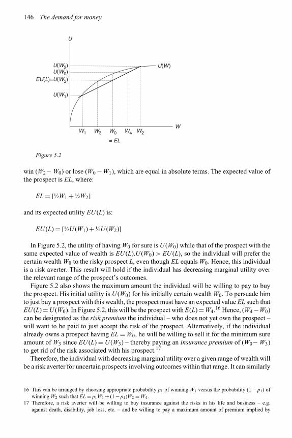
146 The demand for money
W
U(W )
W1 W0
= EL
W2W3
U
U(W2)U(W0)
EU(L)=U(W3)
U(W1)
W4
Figure 5.2
win (W2− W0) or lose (W0 −W1), which are equal in absolute terms. The expected value ofthe prospect is EL, where:
EL = [½W1 + ½W2]
and its expected utility EU (L) is:
EU (L) = [½U (W1) + ½U (W2)]
In Figure 5.2, the utility of having W0 for sure is U (W0) while that of the prospect with thesame expected value of wealth is EU (L).U (W0) > EU (L), so the individual will prefer thecertain wealth W0 to the risky prospect L, even though EL equals W0. Hence, this individualis a risk averter. This result will hold if the individual has decreasing marginal utility overthe relevant range of the prospect’s outcomes.
Figure 5.2 also shows the maximum amount the individual will be willing to pay to buythe prospect. His initial utility is U (W0) for his initially certain wealth W0. To persuade himto just buy a prospect with this wealth, the prospect must have an expected value EL such thatEU (L) = U (W0). In Figure 5.2, this will be the prospect with E(L) = W4.16 Hence, (W4 −W0)can be designated as the risk premium the individual – who does not yet own the prospect –will want to be paid to just accept the risk of the prospect. Alternatively, if the individualalready owns a prospect having EL = W0, he will be willing to sell it for the minimum sureamount of W3 since EU (L) = U (W3) – thereby paying an insurance premium of (W0− W3)to get rid of the risk associated with his prospect.17
Therefore, the individual with decreasing marginal utility over a given range of wealth willbe a risk averter for uncertain prospects involving outcomes within that range. It can similarly
16 This can be arranged by choosing appropriate probability p1 of winning W1 versus the probability (1 − p1) ofwinning W2 such that EL = p1W1 + (1 − p1)W2 = W4.
17 Therefore, a risk averter will be willing to buy insurance against the risks in his life and business – e.g.against death, disability, job loss, etc. – and be willing to pay a maximum amount of premium implied by

Portfolio selection and speculative demand 147
be shown that the individual with increasing marginal utility over a given range of wealth willbe a risk preferrer for uncertain prospects involving outcomes within that range. Further, theindividual with constant marginal utility over a given range of wealth will be risk-indifferenttowards uncertain prospects involving outcomes within that range. These considerations ledFriedman and Savage (1948) to argue that the individual who buys both insurance for somerisks involving relatively small outcomes and lotteries with very much larger outcomes havinga very small probability must have a segment with decreasing marginal utility, followed by asegment with increasing marginal utility at higher levels of wealth. Subsequent contributionsmodified this to the assertion that the utility function should be defined over (W – W c),where W is the individual’s terminal wealth and W c is his existing or customary level ofwealth.
For the following portfolio selection analysis of the demand for money, the assumptionsfor the individual’s preferences are that: (a) U (W ) is a von Neumann–Morgenstern utilityfunction, (b) U ′(W ) > 0, and (c) U ′′(W ) < 0. As we have shown above, the last assumptionensures that the investor is a risk averter.
5.5 The efficient opportunity locus
5.5.1 Expected value and standard deviation of the portfolio
For simplification, assume that the probability distributions are normal and thereforeonly the expected net worth and its standard deviation are relevant to the individual’sdecision. Further, assume that the individual can hold combinations of only two assets,X1 and X2, in his portfolio. Then, the first two moments of the frequency distributionof his terminal wealth, which is the value of the portfolio at the end of the relevantperiod, are:
μ = μ1x1 +μ2x2 (3′)
σ 2 = σ 21 x2
1 + 2ρ12σ1σ2x1x2 +σ 22 x2
2 (4′)
where:x1 = amount of asset X1
x2 = amount of asset X2
μ = expected value of terminal wealthσ 2 = variance of terminal wealth
The budget constraint on the holdings of the two assets is:
x1 + x2 = W (5)
where W is the individual’s initial wealth and the prices of the two assets have been normalizedat unity to avoid continual usage of the price symbols.
his utility function and the risk in question. If a firm is willing to insure him for the risk for less than thisamount, he will buy the insurance; if the required premium is greater than this amount, he will not buy theinsurance.

148 The demand for money
S
s
B
m
m2W
s2W
Figure 5.3
5.5.2 Opportunity locus for a riskless asset and a risky asset
Assume that the market offers a riskless asset S such that μs > 0 and σs = 0, and a riskyasset X2 with μ2 > μs and σ2 > 0. In this case, the opportunity locus for combinations withany risky asset would also be linear, as shown by the line SB in Figure 5.3. Intuitively, if theindividual holds only the asset S, his yield will be μSW , with σ = 0. If he holds only X2, hisyield to the portfolio would be μ2W , with a risk of σ2W . If he holds half his wealth in S andhalf in X2, he would have μ = (½μsW + ½μ2W ) and σ = ½σ2W .
If the riskless asset M (say “money”) also had a zero return – so that μM = 0 – then theopportunity locus would be from the origin to point B.
5.5.3 Opportunity locus for risky assets
Appendix 2 presents the proper derivation of the opportunity locus between μ and σ for thevarious cases. Suppose the market offers only the two risky assets X1 and X2, with σ1, σ2 > 0.Define x1
∗ = x1/W and x2∗ = x2/W = (1−x1
∗), where x1∗ is the proportion of wealth held in
the first asset. The following argument provides three cases for the shapes of the opportunitylocus between μ and σ .
Perfect positive correlation, i.e. ρ12 = 1 :In this case,
σ 2 = σ 21 x2
1 + 2ρ12σ1σ2x1x2 +σ 22 x2
2 (6)
so that:
σ = σ1x1 +σ2x2
which, along with μ = μ1x1 + μ2x2, gives a linear relationship between μ and σ . Such arelationship is shown by the line AB in Figure 5.4a. For the end-point A, representing thewhole portfolio consisting only of the first asset, we have x1 = 1 and x2 = (1 − x1) = 0, so

Portfolio selection and speculative demand 149
m
sss
A
B
A
B
S
mm
A
B
S
(a) (b) (c)
Figure 5.4
that μ = μ1 and σ = σ1. For the end-point B, representing the whole portfolio consistingonly of the second asset, we have x1
∗ = 0 and x2 = (1 − x1) = 1, so that:
μ = μ2 = k2 + k1σ2
which, along with σ = σ2, provides the point B in Figure 5.4a.
Perfect negative correlation, i.e. ρ12 = −1:
In this case,
σ 2 = σ 21 x2
1 − 2σ1σ2x1x2 +σ 22 x2
2 (6′)
so that:
σ = σ1x1 −σ2x2
Hence, σ = 0 for x1/x2 = σ2/σ1. Hence we can define a riskless composite asset X3 for whichσ3 = 0. It would combine the assets X1 and X2 in the proportions given by x1/x2 = σ2/σ1, withμ3 ={(μ1σ2+μ2σ1)W }/(σ1+σ2) andσ3 = 0. In Figure 5.4b, a portfolio consisting only of X3
is represented by the point S. Now, suppose that we have these three assets (X1, X2, X3) in theportfolio. Combinations of only X1 and X3 in the portfolio yieldσ (X1,X3)= 0 andμ(X1,X3)=μ1X1 +μ3X3, with the linear opportunity locus AS in Figure 5.4b.18 Similarly, combinationsof only X2 and X3 in the portfolio yield σ (X2,X3) = 0 and μ(X2,X3) = μ2x2 + μ3x3, withthe linear opportunity locus SB in Figure 5.4b.
ASB represents the opportunity locus given by the combinations of the two risky assetswith perfect negative correlation.
Opportunity locus for −1 < ρ12 < +1
In the common case where the two assets entail some risk and ρ12 lies between −1 and +1, theopportunity locus will be non-linear and will lie in the area enclosed by ASB in Figure 5.4c.
18 σ in σ (X1,X3) and μ in μ(X1,X3) are being used as functional symbols so that their arguments can clearlyindicate which assets are in the portfolio. However, σ and μ retain their definitions as being respectively thestandard deviation and the expected return to the portfolio.

150 The demand for money
E
A
b
s
m
s
m
a
B
B
A
D
(a) (b)
Figure 5.5
The closer ρ12 is to +1, the closer will this locus be to the line AB. When ρ12 differs from+1, there exist economies in risk from holding a diversified portfolio and the opportunitylocus moves towards ASB.19
Opportunity locus for three risky assets
Now assume that three risky assets X1, X2, X3 are available. Combinations of X1 and X2
alone, of X1 and X3 alone and of X2 and X3 alone, give the opportunity loci in Figure 5.5a asAB, AE and BE respectively. Further, consider combinations of the points a on AB and b onBE. These generate the locus ab. If we were similarly to take combinations of all the otherpoints on AB, AE and BE, the opportunity locus would be the area enclosed by the curveADB in Figure 5.5b. In the general case with more than three risky assets, the opportunitylocus would have a similar shape.
Opportunity locus for one riskless and several risky assets
Consider, further, the possibility that the individual will wish to hold combinations of ariskless asset and the two risky assets. The individual can hold various combinations ofthe risky assets only or hold a combination of the riskless asset with some combination
19 This can be intuitively illustrated by the folklore that one should not put all one’s eggs in one basket. It paysto divide one’s eggs between two baskets as long as there is a possibility that when one of the baskets falls,the other one may not. If both baskets are guaranteed to fall simultaneously or not fall at all, e.g. when boundtogether, there is no advantage to separating the eggs between the baskets; the same number of eggs will breakwhether they are separated or not. In our formal language, the correlation coefficient of the baskets falling isone and there are no economies. However, if it is guaranteed or certain that when one basket falls, the otherwill not – as when the baskets are at the opposite ends of a pole carried across one’s shoulders – separatingthe eggs into the two baskets will ensure that some eggs will with certainty escape breakage. In this case, thecorrelation coefficient of the baskets falling is (−1). In the intervening cases, the eggs should be divided betweenthe baskets, the exact division depending upon the probability that when one basket falls, the other will not – thatis, upon the correlation coefficient between the baskets falling. Similarly, the individual investor must considerthe correlation coefficient of net worth between the assets since he may be able to reduce his risk through thediversification of the portfolio between the assets.
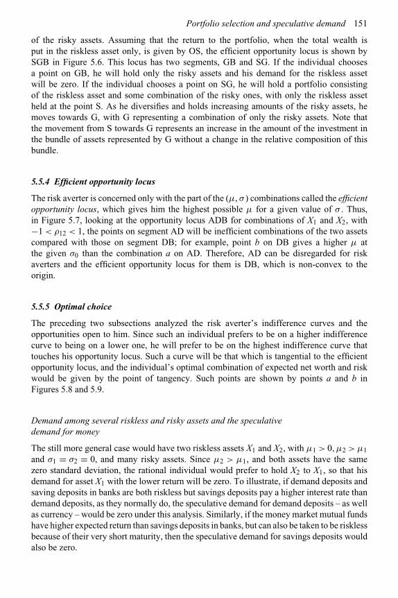
Portfolio selection and speculative demand 151
of the risky assets. Assuming that the return to the portfolio, when the total wealth isput in the riskless asset only, is given by OS, the efficient opportunity locus is shown bySGB in Figure 5.6. This locus has two segments, GB and SG. If the individual choosesa point on GB, he will hold only the risky assets and his demand for the riskless assetwill be zero. If the individual chooses a point on SG, he will hold a portfolio consistingof the riskless asset and some combination of the risky ones, with only the riskless assetheld at the point S. As he diversifies and holds increasing amounts of the risky assets, hemoves towards G, with G representing a combination of only the risky assets. Note thatthe movement from S towards G represents an increase in the amount of the investment inthe bundle of assets represented by G without a change in the relative composition of thisbundle.
5.5.4 Efficient opportunity locus
The risk averter is concerned only with the part of the (μ, σ ) combinations called the efficientopportunity locus, which gives him the highest possible μ for a given value of σ . Thus,in Figure 5.7, looking at the opportunity locus ADB for combinations of X1 and X2, with−1 < ρ12 < 1, the points on segment AD will be inefficient combinations of the two assetscompared with those on segment DB; for example, point b on DB gives a higher μ atthe given σ0 than the combination a on AD. Therefore, AD can be disregarded for riskaverters and the efficient opportunity locus for them is DB, which is non-convex to theorigin.
5.5.5 Optimal choice
The preceding two subsections analyzed the risk averter’s indifference curves and theopportunities open to him. Since such an individual prefers to be on a higher indifferencecurve to being on a lower one, he will prefer to be on the highest indifference curve thattouches his opportunity locus. Such a curve will be that which is tangential to the efficientopportunity locus, and the individual’s optimal combination of expected net worth and riskwould be given by the point of tangency. Such points are shown by points a and b inFigures 5.8 and 5.9.
Demand among several riskless and risky assets and the speculativedemand for money
The still more general case would have two riskless assets X1 and X2, with μ1 > 0,μ2 > μ1
and σ1 = σ2 = 0, and many risky assets. Since μ2 > μ1, and both assets have the samezero standard deviation, the rational individual would prefer to hold X2 to X1, so that hisdemand for asset X1 with the lower return will be zero. To illustrate, if demand deposits andsaving deposits in banks are both riskless but savings deposits pay a higher interest rate thandemand deposits, as they normally do, the speculative demand for demand deposits – as wellas currency – would be zero under this analysis. Similarly, if the money market mutual fundshave higher expected return than savings deposits in banks, but can also be taken to be risklessbecause of their very short maturity, then the speculative demand for savings deposits wouldalso be zero.

152 The demand for money
m
s
B
A
S
O
G
Figure 5.6
m
s
B
A
D
b
a
s0
Figure 5.7
The optimal point a in Figure 5.8 is a combination of the riskless asset and the standardbundle of risky assets represented by point G.20 The optimal point b in Figure 5.9 is acombination of the risky assets A and B only, while the riskless asset S is not held. A changein preferences that leaves the individual on the segment GB of the opportunity locus willchange the relative demands for the risky assets A and B, but still without a positive demandfor the riskless asset S. However, the individual whose initial optimal choice does not includethe riskless asset may shift partly or wholly into the riskless asset, either because of an increasein his degree of risk aversion – which would shift the indifference curves – or because of anincrease in the riskiness, or decrease in the expected net worth, of the risky assets – whichwould shift the efficient opportunity locus.
20 A shift in the degree of risk aversion that changes the slope of the indifference curves in the neighborhood ofpoint a but leaves the optimal combination on the segment CG will change the demand for the riskless assetand the risky bundle. It will, however, leave the composition of the risky bundle unchanged. Such a shift inpreferences was termed by Hicks a change in the degree of liquidity preference.
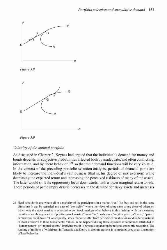
Portfolio selection and speculative demand 153
m
s
B
S
a
G
A
Figure 5.8
m
s
B
AS
Gb
Figure 5.9
Volatility of the optimal portfolio
As discussed in Chapter 2, Keynes had argued that the individual’s demand for money andbonds depends on subjective probabilities affected both by inadequate, and often conflicting,information, and by “herd behavior,”21 so that their demand functions will be very volatile.In the context of the preceding portfolio selection analysis, periods of financial panic arelikely to increase the individual’s cautiousness (that is, his degree of risk aversion) whiledecreasing the expected return and increasing the perceived riskiness of many of the assets.The latter would shift the opportunity locus downwards, with a lower marginal return to risk.These periods of panic imply drastic decreases in the demand for risky assets and increases
21 Herd behavior is one where all or a majority of the participants in a market “run” (i.e. buy and sell in the samedirection). It can be regarded as a case of “contagion” where the views of some carry along those of others onwhich way the stock market is expected to go. Stock markets often behave in this fashion, with their extrememanifestations being labeled, if positive, stock market “mania” or “exuberance” or, if negative, a “crash,” “panic”or “nervous breakdown.” Consequently, stock markets suffer from periodic overvaluations and undervaluationsof stocks relative to their fundamental values. What happens during these episodes is sometimes attributed to“human nature” or “animal spirits,” implying that it is beyond explanation by rational economic reasoning. Therunning of millions of wildebeest in Tanzania and Kenya in their migrations is sometimes used as an illustrationof herd behavior.

154 The demand for money
in the demand for the riskless asset. Such shifts in demand may be self-reinforcing for sometime since the fall in the demand for risky assets would lower their prices, causing a capitalloss from the holdings of these assets. If these developments also cause the future expectednet worth of the risky assets to fall and their expected riskiness to increase, the opportunitylocus would shift down further, so that the optimal combination, with given preferences, willinclude still more of the riskless asset and even less of the risky assets. This process of declinein the net worth of risky assets and increased demand for the riskless asset could prove to bea cumulative one for some time.
In periods of optimism and a boom in asset prices, the opposite process is likely to occur.This would mean a decrease in demand for the riskless asset and an increase in demand forthe risky assets, along with their prices. This movement could also prove to be a cumulativeone for some time.
5.6 Tobin’s analysis of the demand for a riskless assetversus a risky one
In an early form of the preceding analysis, Tobin (1958, pp. 65–86)22 analyzed the demandfor a riskless asset called “money” with a zero rate of return – that is, with a terminal(i.e. end-of-investment-period) value of unity and with zero standard deviation – as againsta risky asset called bonds, with a positive return and a positive standard deviation. Thisanalysis is presented in Figure 5.10, though with the difference that we will use savingsdeposits as our riskless asset – these deposits have a positive but still riskless rate of return.
m
s
BmBW
sBW
S
0
1
sA
a
A
X
Figure 5.10
22 The part of Tobin’s analysis that refers specifically to Keynes’s arguments on the speculative demand waspresented in Chapter 2.

Portfolio selection and speculative demand 155
Figure 5.10 has the expected value μ of terminal wealth on the vertical axis and the standarddeviation σ of wealth on the horizontal axis. If the individual invests his wealth wholly inmoney, he will be at point S. If he invests only in bonds, he will at point B. The efficientopportunity locus is SB. In the bottom part of this figure, designate any point on the verticalaxis as 1. The distance from 0 to any point on the segment 01 measures the proportion ofwealth invested in bonds. The line from the origin down to the point given by (1, σBW ) is 0X.
If the individual chooses the point A, he will purchase σA, which implies, as shown in thebottom part of Figure 5.10, that he will place the proportion 0a in bonds and the proportiona1 in savings deposits.
We can use Figure 5.10 to investigate the effects of changes in the opportunity locus orthe indifference curves. We consider three examples of the former.
(i) The first example considers a portfolio composed of a riskless asset with a positive returnand a risky asset with a higher return. Assume that the tax authorities impose a lump-sumtax on a positive return to the portfolio, without a loss offset for investors incurring losses,in a manner such that the opportunity locus shifts down in a parallel fashion, as shown bythe shift from SB to S′B′ in Figure 5.11.23 Under this assumption, the particular shape of theindifference curves drawn in Figure 5.11 leads to an increase in the optimal purchase of riskto 0σa′ , so that the proportion invested in bonds increases to 0a′. This proportion is greaterthan the initial proportion 0a.
With S′B′ parallel to SB, the marginal rate of substitution (∂μ/∂σ ) between the expectedreturn and risk does not change. Hence, the substitution effect between them does not occurand the only effect in operation is the “income effect” – really a wealth effect in the contextof portfolio selection – which could go either way, so that the after-tax optimal demand for
m
s
B
sBW
S
S′
1
a
B′
a′
A
A′
X
sa′sa
Figure 5.11
23 This assumes that the tax does not change the standard deviation of terminal wealth.
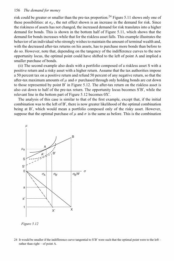
156 The demand for money
risk could be greater or smaller than the pre-tax proportion.24 Figure 5.11 shows only one ofthese possibilities: at σa′ , the net effect shown is an increase in the demand for risk. Sincethe riskiness of assets has not changed, the increased demand for risk translates into a higherdemand for bonds. This is shown in the bottom half of Figure 5.11, which shows that thedemand for bonds increases while that for the riskless asset falls. This example illustrates thebehavior of an individual who strongly wishes to maintain the amount of terminal wealth and,with the decreased after-tax returns on his assets, has to purchase more bonds than before todo so. However, note that, depending on the tangency of the indifference curves to the newopportunity locus, the optimal point could have shifted to the left of point A and implied asmaller purchase of bonds.
(ii) The second example also deals with a portfolio composed of a riskless asset S with apositive return and a risky asset with a higher return. Assume that the tax authorities imposea 50 percent tax on a positive return and refund 50 percent of any negative return, so that theafter-tax maximum amounts of μ and σ purchased through only holding bonds are cut downto those represented by point B′ in Figure 5.12. The after-tax return on the riskless asset isalso cut down to half of the pre-tax return. The opportunity locus becomes S′B′, while therelevant line in the bottom part of Figure 5.12 becomes 0X′.
The analysis of this case is similar to that of the first example, except that, if the initialcombination was to the left of B′, there is now greater likelihood of the optimal combinationbeing at B′, which would mean a portfolio composed only of the risky asset. However,suppose that the optimal purchase of μ and σ is the same as before. This is the combination
m
s
B
sBW
S
S′0
1
sA sB′
a
A
B′
X′ X
a′
mA
A′
Figure 5.12
24 It would be smaller if the indifference curve tangential to S′B′ were such that the optimal point were to the left –rather than right – of point A.

Portfolio selection and speculative demand 157
indicated in Figure 5.12 by the point A′, which now implies a higher proportion (indicatedby point a′) of the portfolio held in bonds and a smaller one in the riskless asset. Hence,although the tax reduced the after-tax return on bonds and the optimal combination of μ andσ remains the same, the amount invested in bonds increases because bonds now yield a lowerreturn and risk. In this example, the substitution effect is again zero since the slope of theopportunity locus S′B′ is the same as that of SB, so that the income effect alone determinesthe changes in the desired holdings of money and bonds.
(iii) For the third example, assume, as in Tobin, that the riskless asset has a zero return.Tobin called such an asset “money.” The relevant Figure is now Figure 5.13, with the initialopportunity locus being 0B. Further, assume that the tax authorities impose a 50 percent taxon the average rate of return on investments, without a loss offset for investors incurringlosses, such that the post-tax opportunity locus becomes 0B′. Both income and substitutioneffects occur in this case. The optimal point in this figure becomes A′, so that the purchase ofrisk becomes 0σa′ , implying that the proportion invested in bonds falls to 0a′. This proportionis less than the initial proportion 0a, contrary to the situation shown in Figures 5.11 and 5.12.In this example, the nature of the indifference curves is drawn such as to imply an increaseddemand for the riskless asset.
The difference between Figures 5.11 and 5.13 is that the slope (∂μ/∂σ ) of the opportunitylocus has shifted in the latter but not in the former. In Figure 5.13, the imposition of the taxreduces the marginal return to risk-taking – measured as ∂μ/∂σ – so that the substitution effectcomes into play and will cause a reduction in the optimal amount of the risk bought throughbond purchases. Although the income effect could go either way, Figure 5.13 assumes that thetwo effects are in the same direction or that the substitution effect in favor of purchasing lessrisk dominates an opposing income effect. Since less risk is bought at A′, and the riskinessof bonds has not changed, the bottom part of this figure shows that the individual will investa smaller part of the portfolio in bonds.
Figures 5.11 to 5.13 illustrate the use of the general utility function for deriving the demandfor money, assumed to be riskless with zero or positive return, and risky assets. This analysis
m
s
B
sBW0
1
a′
B′
a
A′
A
X
sasa′
Figure 5.13

158 The demand for money
is diagrammatic and implies that the demand for money will depend on the expected returnand standard deviation, as well as on the wealth to be allocated. Shifts in the opportunitylocus because of tax changes or, more generally, because of changes in the perceptions offuture risk and return – as occur periodically in the bond and stock markets – will alter thedemand for money.
Since the preceding analysis has relied only upon indifference curves to representpreferences, its underlying utility function can be taken to be ordinal and need not be cardinalin the Neumann–Morgenstern sense. Current portfolio analysis is usually mathematical, basedon the expected utility hypothesis, and tends to use specific cardinal utility functions. Thenext section presents this type of analysis.
5.7 Specific forms of the expected utility function
5.7.1 EUH and measures of risk aversion
If we look at the preceding indifference curve analysis, based on the mean–variance approachto portfolio selection, a suitable measure of risk aversion would seem to be ∂μ/∂σ . However,this measure does not directly relate to the form of the utility function that has wealth as itsargument, and we sometimes want one that does so.
As shown above by Friedman–Savage analysis of Section 5.4 relating the slope of the utilityfunction U (W ) to risk aversion, risk aversion is implied by the decrease in the marginal utilityof wealth, so that one measure of risk aversion would be U ′′(W ), which is the change in themarginal utility of wealth. However, U ′′(W ) is not invariant to the admissible transformationsof the utility function,25 as we show in the next few paragraphs.
Cardinality of the von Neumann–Morgenstern utility function
As mentioned earlier, the von Neumann–Morgenstern (N–M) utility function is based on a setof axioms (see Appendix 1) which imply that, for an individual whose preferences obey theaxioms, the utility function will be “unique up to a linear transformation.” That is, given anN–M utility function U (W ) for such an individual, we can construct another utility functionV (W ) with identical indifference curves by a linear transformation, as in:
V (W ) = a + bU (W ) b > 0 (7)
In constructing V (W ) from U (W ), a and b can be given any arbitrary values as long asb is positive. V (W ) is an equally valid utility function for an individual having U (W ), andthe indifference curves for both U (W ) and V (W ) are identical. However, their derivativesdo differ in value, since:
V ′(W ) = bU ′(W ) (8)
V ′′(W ) = bU ′′(W ) (9)
25 For ordinal utility functions, even the sign of U ′′(W ) can change under admissible (increasing) transformationsof the utility function, so that it does not make sense to talk of decreasing marginal utility for them. For cardinalfunctions, the sign remains invariant under admissible (linear) transformations but the magnitude can change.

Portfolio selection and speculative demand 159
where ′ designates the first-order derivative and ′′ designates the second-order one. Note thatby the assumptions specifying a risk averter’s preferences, U ′ and V ′ > 0 while U ′′ andV ′′ < 0. The above equations imply that:
V ′′(W )/V ′(W ) = U ′′(W )/U ′(W ) (10)
Hence, U ′′/U ′ is not altered by admissible transformations of the N–M utility function. Thisproperty makes this ratio, as against U ′′ alone, appealing as a measure of the degree of riskaversion implied by the given utility function U (W ).
Measures of risk aversion
In (10), U ′ > 0, U ′′ < 0 and U ′′/U ′ < 0, so that the degree of risk aversion is usually measuredby [−U ′′/U ′], which gives a positive value. [−U ′′/U ′] is called the absolute degree of riskaversion.
Since U ′ and U ′′ are unlikely to increase or decrease proportionately with wealth,[−U ′′/U ′] will be affected by the amount of wealth. In order to ensure that the degree of riskaversion is independent of the level of wealth, another popular measure of the degree of riskaversion is [W .U ′′/U ′]. This measure is independent of the level of wealth, as well as of thearbitrary constants a and b.[−W .U ′′/U ′] is called the relative degree of risk aversion.
The absolute and relative degrees of risk aversion can be calculated for any twice-differentiable utility function. While there is no a priori reason to expect that either of thesewill be constant for any given individual’s particular utility function, the utility functions forwhich such constancy holds are analytically convenient to use and are therefore popular ineconomic analysis. We examine these in turn, and will follow them with a presentation ofthe quadratic utility function, which does not have the constancy of either the absolute orthe relative degree of risk aversion but was used in some early expositions of the speculativedemand for money.
5.7.2 Constant absolute risk aversion (CARA)
Constant absolute risk aversion (CARA) requires that:
−U ′′(W )/U ′(W ) = γ γ ≥ 0 (11)
where γ is the constant degree of ARA. Hence,
U ′′(W ) = −γ U ′(W ) (11′)
Since U ′′(W ) is a second-order derivative, integrating both sides of (11′) gives the utilityfunction itself, though with two integrating constants which would have been dropped in thedifferentiation process. The utility function given by integrating (11) twice26 is:
U (W ) = a − b exp(−γ W ) (12)
26 CARA requires that:
U ′′(W ) = −γ U ′(W )

160 The demand for money
Assuming that W is normally distributed with mean μ and standard deviation σ , as before,the expected value of this utility function is given by:
EU (W ) = a − b[exp(−γμ+ ½γ 2σ 2)] (13)
Since b > 0 and γ ≥ 0, maximizing the expected utility function (13) is equivalent tominimizing [exp(−γμ+ ½γ 2σ 2)] or maximizing:
(μ− ½γ σ 2) (14)
In (14), substituting μ = �iμixi and σ 2 = �i�jρijσiσjxixj restates the decision problem as:
Maximize {�iμixi − ½γ (�i�jρijσiσjxixj)} i, j = 1, . . . ,n
subject to:
�ixi = W (15)
Note that xi is the amount of the ith asset, not its proportion to wealth. Equation (15) representsone of the simplest decision frameworks in portfolio selection analysis, which is the mainreason for its usage in such analysis. Note its main assumptions: the frequency distributionof terminal wealth W is normal, the individual’s preferences satisfy the N–M axioms and thedegree of absolute risk aversion is constant. The following analysis applies this analysis tothe case of two risky assets.
CARA and the choice between two risky assets
Assume in the context of (15) that the individual’s choice is between different quantities ofthe two risky assets X1 and X2 so that n = 2. His decision problem can be stated as:
Maximize (μ1x1 +μ2x2) −{½γ (σ11x21 + 2σ12x1x2 +σ22x2
2)}
subject to:
x1 + x2 = W (16)
Hence, integrating both sides of this equation specifies that:
ln U ′(W ) = k1 − γ W
so that:
U ′(W ) = exp(k1 − γ W )
Integrating again,
U (W ) = k2 − (1/γ ) exp(k1 − γ W ) = a − b exp(−γ W )
where k1 and k2 are constants of integration, a = k2 and b = (1/γ )exp(k1).

Portfolio selection and speculative demand 161
The Lagrangian function L for this problem is:
L = (μ1x1 +μ2x2) −{½γ (σ11x21 + 2σ12x1x2 +σ22x2
2)}+λ[x1 + x2 − W ] (17)
where λ is the Lagrangian multiplier. The first-order conditions for maximizing L with respectto x1, x2 and λ are:
∂L/∂x1 = μ1 − γ (σ11x1 +σ12x2) +λ = 0
∂L/∂x2 = μ2 − γ (σ22x2 +σ12x1) +λ = 0
∂L/∂λ = x1 + x2 − W = 0
These conditions yield the optimal holdings of the two assets as:
x1 = k1 + k2W (18)
x2 = −k1 + (1 − k2)W (19)
where:
k1 = (μ1 −μ2)/γ (σ11 − 2σ12 +σ22)
k2 = (σ22 −σ12)/(σ11 − 2σ12 +σ22)
so that the demand for each risky asset increases with wealth but the proportions of the twoassets in the portfolio change as initial wealth W increases. These demand functions dependupon the expected returns and the variances and covariances.
CARA and the special case when a riskless asset is available
If X1 were a riskless asset, i.e. with σ1 = 0, while X2 was still a risky asset, note thatσ11 = σ12 = 0. Inserting these in the demand functions (18) and (19) implies that:
x1 = W − (μ2 −μ1)/(γ σ22) (20)
x2 = (μ2 −μ1)/(γ σ22) (21)
where x2 (the demand for the risky asset) is independent of initial wealth, so that any increasesin the initial wealth (beyond a certain level specified by (μ2 −μ1)/( γ σ22)) will be completelyadded to the riskless asset holdings. That is, for W ≥ (μ2 − μ1)/(γ σ22), ∂x1/∂W = 1 and∂x2/∂W = 0. The amount of wealth held in the risky asset will stay unchanged as wealthincreases beyond the amount specified by (21), so that, as the investor becomes wealthier,the proportion of his optimal portfolio allocated to the riskless asset will increase. This is farfrom the behavior pattern of most investors, who increase their holdings of the risky assetsas their wealth increases. Financial markets now provide several riskless assets such as M1,savings deposits, money market mutual funds, etc., so that CARA implies that, beyond acertain amount of wealth, increases in wealth will be added to the riskless asset holdings, sothat their proportion relative to wealth will increase. This prediction makes CARA especiallyunrealistic for portfolio allocation behavior. This result also holds if there is at least oneriskless asset but several risky ones.
Hence, a CARA utility function, though analytically convenient, is not appropriatefor the derivation of the speculative/portfolio demand function for M1, M2 or other

162 The demand for money
monetary aggregates, all of which include a riskless component, nor for the derivation ofthe portfolio demand for risky assets.
Limitation of CARA as a utility function for general portfolio selection
On a more general note, CARA implies that the investor becomes increasingly reluctant totake risks as he gets richer, so that he invests in increasing proportions of the less risky assetsand decreasing proportions of the riskier assets. Intuitive knowledge of investor behaviorindicates the opposite; most investors tend to be rather more cautious with limited wealthand become more willing to take chances as their wealth increases. Hence, CARA cannotbe taken to be plausible for the choice among assets and its use in this sphere is mainly dueto its analytical convenience. Constant relative risk aversion (CRRA) is more realistic in itsimplications for the demand for assets. We now turn to its analysis.
5.7.3 Constant relative risk aversion (CRRA)
Relative risk aversion (RRA) is specified by:
RRA = [−W .U ′′/U ′] (22)
Constant relative risk aversion (CRRA) is the requirement that:
[−W .U ′′/U ′] = β (23)
where β is the constant coefficient of RRA. Integrating both sides of this equation twice leadsto the utility function (Cuthbertson, 1985, Ch. 3):
U (W ) = a − bW 1−β b > 0, β = 1 (24)
= ln W for β = 1 (25)
where a and b are the constants of integration.27 β is known as the Arrow–Pratt measure ofrelative risk aversion.
27 CRRA is often used in intertemporal consumption analysis, where the intertemporal utility function is assumedto be time separable and is specified as:
U (c0,c1, . . . ,cT ) = �tu(ct )/(1 − δ)−t t = 0,1, . . . ,T
where U is the intertemporal utility function and u is the period utility function. δ is the rate of time preference.u is assumed to be a CRRA function of the form:
u(ct ) = (c(1−b)t )/(1 − b) for b > 0,b = 1
= ln ct for b = 1
For these functions, the elasticity of substitution between consumption in any two periods is constant andequal to 1/b.
The corresponding period utility function for CARA is:
u(ct ) = −(1/a) exp(−act ) a > 0

Portfolio selection and speculative demand 163
In (25), U (W ) = ln W is analytically very tractable and is probably the most popular formof the von Neumann–Morgenstern utility function. Its degrees of absolute and relative riskaversion are:
ARA = 1/W
RRA = 1
so that the absolute degree of risk aversion decreases as the investor gets richer. This is alsotrue of the general form of the CRRA utility function.
CRRA and the choice among risky assets
If there are only risky assets, maximizing the expected value of the CRRA utility functionsubject to the budget constraint yields the demand function for the ith risky asset as:
xi/W = kiμ i = 1,2, . . . , n (26)
where:
ki = ki(β,μ,σ ij)
The variables in bold type indicate the vectors of the relevant variables (Cuthbertson, 1985,Ch. 3). Equation (26) implies that the proportions of the risky and riskless assets in theportfolio remain unchanged as wealth increases, so that the elasticity of the demand for eachasset with respect to wealth is unity.
CRRA and the demand functions for monetary aggregates
If the first asset is riskless while the others are all risky, the demand function implied by (26)for the riskless asset is:
x1/W = 1 −�i(xi/W ) i = 2, . . . , n
= 1 −�ikiμi
(27)28
The asset demand functions (26) and (27) are homogeneous of degree one in W , sothat the proportions of the riskless and each of the risky assets in the portfolio remainconstant as the portfolio grows. Alternatively stated, the individual’s portfolio demand foreach asset, whether riskless or risky, has an elasticity of unity with respect to his wealth,which is much more plausible than the implication of CARA for the demand for themonetary aggregates. However, casual intuition does suggest that in financially developedeconomies the individual’s demands for currency and even demand deposits do not increaseproportionately with his wealth, so that CRRA may not be suitable for deriving the portfoliodemand for M1. This is not necessarily so for the other components, M2, M3 and so on,for which CRRA may perform better. The usefulness of CRRA for predicting the demand
28 See Cuthbertson (1985, Ch. 3) for the derivations of this and earlier results on the CRRA utility function.

164 The demand for money
functions for M1, M2 and wider monetary aggregates will, therefore, vary with the aggregatein question, but will not be appropriate for their common element, which is M1. However,as we discuss later in this chapter, the portfolio demand for M1 may, in fact, be zero in themodern economy.
5.7.4 Quadratic utility function
Besides CARA and CRRA, the third type of utility function in common usage in portfolioselection theory is:
U (W ) = a + bW − cW 2 a,b,c > 0 (28)
Hence,
EU (W ) = a + bμ− cE(W 2) (29)
where, by the definition of σ 2,
σ 2 = E(W −μ)2 = E(W 2 − 2W .μ+μ2)
= EW 2 − 2EW .μ+μ2 = E(W 2) − 2μ2 +μ2
= (EW 2) −μ2
Therefore,
E(W 2) = μ2 +σ 2 (30)
Hence, from (29) and (30),
EU (W ) = a + bμ− cμ2 − cσ 2 a,b,c > 0 (31)
The individual maximizes (31) (subject to the budget constraint) with respect toμ andσ . Toderive the asset demand functions, substitute the equations for μ and σ in (31) and maximizethe resulting expected utility function with respect to the quantities of the assets. Since thequadratic utility function does not possess the CRRA property, the proportions of the assetswill not remain constant as wealth increases.
The quadratic utility function is a second-degree polynomial in W . Such a polynomialtransforms to an expected utility function in the first two moments of the probabilitydistribution of wealth. Polynomials of higher degree can also be used as utility functions.These would bring into the expected utility function the other moments of the probabilitydistribution, which is desirable, but they are usually quite intractable for analysis.
Limitations of the quadratic utility function
Since the utility function must have positive marginal utility of wealth, it must satisfy∂U/∂W = b − 2cW > 0, which requires that W < 2c/b. This restriction severely limitsthe range over which the quadratic utility function is applicable.
Portfolio selection and speculative demand 165
Further, for the quadratic utility function in (28), the absolute degree of risk aversion(ARA) is given by:
ARA = −U ′′(W )/U ′(W ) = 2c/(b − 2cW )
Since (b−2cW ) > 0, the ARA for the quadratic utility function is positive and increasing inW , so that as the investor gets wealthier, he becomes more risk averse. This increase – ratherthan a decrease – makes the quadratic utility function even less appealing than the CARA,but, as shown above, the latter has its own limitations.
To conclude, the CARA and quadratic utility functions are inappropriate for the analysisof the portfolio demand for money and bonds, while CRRA is more suitable.29
5.8 Volatility of the money demand function
Note that the speculative demand for money and the coefficients of its independent variableswill depend upon the means, the standard deviations and the correlation coefficients of theexpected terminal values of the assets, for all of which the subjectively expected futureand not the past actual values are the relevant ones. Keynes (1936, Ch. 13) argued that theexpected bond yields and equity prices depend on the mood of the market participants andtheir perceptions of the future, which are often based on very limited information and subjectto the “herd instinct.” These elements of the financial markets are as much in evidence todayas in Keynes’s day, as the daily movements of the stock market indices clearly indicate.
These arguments imply that the demand functions for bonds and equities are constantlyshifting, so that they could not be properly estimated or, if estimated, would be worthless –unless the nature of the shift could be specified and adjustments made for it. If we followKeynes’s analysis, presented in Chapter 2 above, of bulls and bears for the speculative demandfor money, this demand function must also be similarly volatile.
Empirical studies, reported in Chapter 9, do not generally estimate a speculative demandfor money separately from the demand for real balances as a whole. While these studiessometimes show instability of the demand function for money as a whole over time, theydo not show the sort of high volatility, due to sudden shifts in expectations, suggested byKeynes. Further, although considerable shifts in the estimated functions have been observedby studies using an annual or quarterly date in recent years, they seem to have been mainlydue to innovations in transactions technology.
5.9 Is there a positive portfolio demand for money balances in themodern economy?
The modern economy with a well-developed financial sector has a plethora of financialassets that are as riskless as currency and demand deposits, or close enough in riskiness notto matter much to the individuals in the economy. Among these assets are various typesof savings deposits, term deposits, certificates of deposit (CDs) and very short-term moneymarket instruments. Since they pay higher returns than M1 without an accompanying higher
29 However, this assertion does not necessarily mean that its implications for asset demand functions are valid.It is commonly believed that the wealthier investors are, ceteris paribus, less risk averse. If so, their degree ofrelative risk aversion would not be constant but decreasing.

166 The demand for money
risk, M1 will not be part of the efficient opportunity locus and will not be demanded forspeculative purposes (Chang et al., 1983). Similarly, there will be a portfolio demand onlyfor the savings deposits component of M2, as long as other riskless assets in the economy donot dominate these deposits in expected return.
Consequently, in economies with a variety of riskless assets which are riskless in nominalterms but which do not directly circulate as a medium of exchange and are therefore not partof narrow money, the speculative demand for M1 (which is the medium of exchange butpays a lower rate of interest) would be non-existent or confined to those individuals who donot have access to other riskless assets at a low enough cost. Hence, the speculative demandmodel may be generally applicable – and the speculative demand for narrow money maybe positive – in economies with poorly developed financial institutions and markets, whereother riskless assets do not exist or do not dominate over money in their return. However, thismodel no longer seems applicable to the M1 holdings of the common households, firms andfinancial institutions in the modern developed economy. In such a context, while there may bea significant and large speculative demand for certain forms of savings deposits and for moneymarket instruments, there need not be a significant demand for currency and demand deposits.
In terms of the general evolution of the financial sectors in Western economies, theincreasing proliferation of banks since the 1950s, accompanied by a considerable increasein the ease of transfer from savings accounts to checking accounts, especially in the banks,have brought about an increasing dominance of the net return (over transfer costs) on savingsdeposits and a continuing increase in the proportion of savings to M1, with a correspondingincrease in the M2/M1 ratio. The innovation of automatic tellers and their spread in the 1980shastened this movement, so that M1 now tends to be quite small relative to M2 in economieswith developed financial systems.
In more recent years, in the North American and European economies, it has becomepossible to buy and sell almost without notice, and without significant brokerage costs,various types of mutual funds through commercial banks. Among these, the money marketfunds, with investments in Treasury Bills of a month’s or a few months’ maturity, are virtuallyriskless and offer a higher yield than most savings deposits, which are often held in the samefinancial institution. The preceding analysis implies that the ratio of M2 (which excludessuch money market funds) to a still wider definition of money is also likely to decline.
The inventory analysis of transactions demand for money, including M1, and bonds in thepreceding chapter had implied positive demand levels for both these assets. This analysis hadshown the brokerage costs of transactions in and out of bonds, as well as the nominal interestrate, to be a major determinant of these demands. This chapter provides the portfolio demandfor these assets, but ignores brokerage costs and the medium-of-payments role of money.Few models combine both the transactions and portfolio demands in a single, coherent andtractable analysis. However, we can still intuitively examine the impact of the medium-of-payments role of money and of brokerage costs on the portfolio demands for money and bonds.
First, consider the medium-of-payments role of money in the context of portfolio switches.In this role, bonds trade against money, but not directly against commodities, and sales ofone type of bond do not occur simultaneously with the purchase of another type of bond. Thedelay may be due to institutional practices30 or to the investor’s inertia in making purchaseseven after the funds have appeared in the investor’s accounts. Money is held in the interval
30 For example, many brokerage firms credit customers’ accounts with the funds some days after a sale of bondsoccurs.

Portfolio selection and speculative demand 167
between sales and purchases, so that positive balances, related to transactions, are held inthe management and switches of portfolios. In addition, switches among bonds involve twotransactions, each incurring transactions costs, while a switch from money to bonds involvesonly one transaction, so that for very short holding periods of some bonds it might be profitableto hold money rather than bonds.
Therefore, overall, the portfolio demand for money would depend on the risk and returnfactors encompassed in the mean–variance analysis and the nature of the payments systemrelevant to switches among risky assets, as well as brokerage costs in such switches. Inany case, in the presence of several interest-paying riskless assets, the portfolio demand fornon-interest-paying money balances is likely to be relatively small and more likely to besignificant for small investors than for financial institutions themselves.
Conclusions
Keynes introduced the speculative demand function for money into the literature, andFriedman embedded aspects of the demand for money as a temporary abode of purchasingpower in neoclassical money demand analysis. This role of money occupied centre stagein the analysis of the demand for money for several decades and was used to show thedependence of the demand for money on the rates of interest. The varieties of the analyticaldevelopments discussed in this chapter are testimony to the importance of the speculativemotive in the literature on monetary economics.
The demand function for speculative balances derived in this chapter includes, among itsarguments, wealth (rather than current income) and the expected yields (rather than actualyields) on the available assets. Such a function would be stable in an unchanging environmentbut could be unstable in periods of volatility in the bond and stock markets, changes in financialregulations, innovations in the characteristics of existing assets and the creation of new ones,and changes in the payment mechanisms.
The applicability of this analysis to the demand for money in the modern economy needsto be carefully reconsidered. Keynes’s analysis was based on only money – the only availableliquid and riskless asset – and consols. In such a context, the uncertainty of the terminal valueof consols would create a demand for money in the economy. But developed economies sinceKeynes’s day have created a wide variety of riskless assets that pay positive rates of interest.In these economies, economic units with access to such assets would prefer to hold them astemporary abodes of purchasing power for speculative purposes rather than holding currencyand demand deposits, which either do not pay interest or pay lower rates of interest thanriskless savings accounts. Therefore, the demand for M1 – and even for wider definitions ofmoney such as M2, whose savings deposit component now faces competition from moneymarket funds – must come from transactions and precautionary motives rather than fromspeculative motives. The transactions demand analysis was presented in Chapter 4 and theprecautionary demand analysis will be presented in Chapter 6. A related topic is that of thebuffer stock role of money, which is analyzed in Chapter 6.
Appendix 1
Axioms and theorem of the expected utility hypothesis
This appendix gives one version of the N–M axioms and theorem (Handa, 1983). Define aprospect (also called a lottery or gamble) (x, p) as one having the outcomes x(= x1,x2, . . . ,xn)

168 The demand for money
with respective probabilities of p(= p1,p2, . . . ,pn). The prospects (q, r) and (z, r) aredefined correspondingly. is the symbol for “not preferred to” and = stands for “isindifferent to.”
Axiom 1 (Ordering)
(x,p) (y,q) or (y,q) (x,p).
If (x,p) (y,q) and (y,q) (z,r), then (x,p) (z,r).
Axiom 2 (Continuity)
If (x,p) (y,q) and (y,q) (z,r), then there is some value b,0 < b < 1, for which
(y,q) = (x,z;bp, (1 − b)r).
Axiom 3 (Scale)
For 0 < a < 1, (x,ap) (y,aq) if and only if (x,p) (y,q).
Axiom 4 (Independence)
Given axiom 3, for (x,z;ap, (1 − a)r) (y,z;aq, (1 − a)r) if and only if (x,p) (y,q).
Theorem :The individual’s preferences, under the N–M axioms (1) to (4), can be defined over prospects(x, p) by a utility function of the form pv(x), where pv(x) =∑piv(xi).
Proof :Let M and N be such that (M , 1)� (xi, 1) for all xi and (N , 1)≺ (xi, 1) for all xi. vM is theprobability of getting M and vN is the probability of getting N . For any prospect (xi, 1),since N ≺ xi ≺ M , there exists, by N–M axioms 1 and 2, a prospect (M , N ; vMi, vNi) suchthat:
(xi,1) = (M ,N ;vMi,vNi)
where vMi and vNi are functions of xi. Hence, by axioms 3 and 4,
(x1,x2, . . .,xn;p1,p2, . . .,pn)
= [(M ,N ;vM1,vN1), (M ,N ;vM2,vN2), . . ., (M ,N ;vMn,vNn);p1,p2, . . .,pn]
= (M ,N ;vM1p1 + vM2p2 +·· ·+ vMnpn,vN1p1 + vN2p2 +·· ·+ vNnpn)
where �ivNipi = 1 − �ivMipi, so that∑
i vMipi can be treated as a utility index of theprospect (x, p), with M and N representing two degrees of freedom. vMi = vM (xi).Hence, the N–M utility index of the prospect (x, p) is Epiv(xi) or, more compactly, pv(x).(Q.E.D.)

Portfolio selection and speculative demand 169
Axioms 1 and 2 provide the basis for an ordinal utility function, while axioms 3 and 4lend the utility function its N–M cardinality. Note that there are numerous empiricalcounterexamples in the literature, from both experimental economics and clinical psychology,showing the violation of one or more of these axioms by both ordinary individuals andtheir committed exponents. The focus of objections is often to axiom 4, which embodiesaxiom 3. However, the problem often lies with axiom 3, which leads to the linearity of theexpected utility function in probabilities.31 It is intuitively doubtful whether economic choicesfollow such linearity, especially as we approach the limits of 0 and 1 for probabilities. Suchlinearity of utility in probabilities limits the attitude to risk – for instance, the degree of riskaversion – to the slope of the utility function under certainty, as can be seen from the absoluteand relative measures of risk aversion, as well as from the Friedman and Savage (1948)arguments, which were used in this chapter to derive the attitude to risk solely from the slopeof the utility function under certainty. Consequently, in the expected utility hypothesis, riskaversion cannot arise from the potential nonlinearity of the utility function under uncertaintyin probabilities, which is quite likely to occur in economic choices.
Appendix 2
Opportunity locus for two risky assets
Suppose the market offers only the two risky assets X1 and X2, with σ1, σ2 > 0. Definex1
∗ = x1/W and x2∗ = x2/W = (1 − x1
∗), where x1∗ is the proportion of wealth held in the
first asset. This changes the budget constraint to:
x1∗ + x2
∗ = 1 (32)
The expected return μ to the portfolio is now given by:
μ = μ1x1∗ +μ2(1 − x1
∗)
= μ2 + x1∗(μ1 −μ2)
= μ2 + (σ2 −σ2)(μ1 −μ2)/(σ1 −σ2) + x1∗(σ1 −σ2)(μ1 −μ2)/(σ1 −σ2)
Let k1 = (μ1 −μ2)/(σ1 −σ2), so that:
μ = μ2 + (σ2 −σ2)k1 + (σ1 −σ2)k1x1∗
= (μ2 −σ2k1) +σ2k1 +σ1k1x1∗ −σ2k1x2
∗ (33)
Now let k2 = μ2 −σ2k1, with the result that:
μ = k2 + k1{σ1x1∗ +σ2(1 − x1
∗)} (34)
This is a general result for the expected return on the two-asset portfolio.
31 This linearity is clearly evident if the prospect has only two outcomes x1 and 0, so that it is (x1, 0; p1, (1−p1)).

170 The demand for money
(i) Derivation of the opportunity locus for perfect positive correlation (ρ12 = 1)
For ρ12 = +1, we have:
σ = σ1x1∗ +σ2x2
∗ (35)
Substituting (35) in (34), we get:
μ = k2 + k1σ (36)
where, as mentioned earlier, k1 and k2 are constants for given values of the means and standarddeviations of the assets. Therefore, in the case of perfect positive correlation between thetwo assets in the portfolio, the relationship between the portfolio’s expected return μ and itsstandard deviation σ is linear, as shown by the line AB in Figure 5.4a.
For the whole portfolio consisting only of the first asset, we have x∗1 = 1 and (1− x∗
1) = 0,so that the preceding equations imply that:
μ = μ1 = k2 + k1σ1
which, along with σ = σ1, provides the point A in Figure 5.4a.For the whole portfolio consisting only of the second asset, we have x∗
1 = 0 and x∗2 =
(1 − x∗1) = 1, so that the preceding equations correspondingly imply that:
μ = μ2 = k2 + k1σ2
which, along with σ = σ2, gives the point B in Figure 5.4a.
(ii) Derivation of the opportunity locus for perfect negative correlation (ρ12 = −1)
In this case,
σ = σ1x1 −σ2x2 (37)
so that σ = 0 for x1/x2 = σ2/σ1.Given (37), we can define a riskless composite asset X3 for which σ3 = 0. It would combine
X1 and X2 in the proportions given by x1/x2 =σ2/σ1, withμ3 ={(μ1σ2 +μ2σ1)W }/(σ1+σ2)and σ3 = 0. Now suppose that we have these three assets (X1, X2, X3) in the portfolio.Combinations of only X1 and X3 in the portfolio yield σ (X1,X3) = 0 and μ(X1,X3) = μ1x1 +μ3x3, with the linear opportunity locus AS in Figure 5.4b.32 Similarly, combinations of onlyX2 and X3 in the portfolio yield σ (X2,X3) = 0 and μ(X2,X3) = μ2x2 +μ3x3, with the linearopportunity locus SB in Figure 5.4b.
32 σ in σ (X1, X3) and μ in μ(X1, X3) are being used as functional symbols, so their arguments can clearly indicatewhich assets are in the portfolio. However, σ and μ retain their definitions as being respectively the standarddeviation and the expected return to the portfolio.

Portfolio selection and speculative demand 171
In terms of the proportions x1∗ and x2
∗(= 1−x1∗) of the portfolio invested in the two assets
with ρ12 = −1, the standard deviation σ of the portfolio is given by:
σ 2 = σ 21 x1
∗2 − 2σ1σ2x1∗x2
∗ +σ 22 x2
∗2
= σ1x1∗ −σ2(1 − x1
∗)
so that, for σ = 0, we have:
x1∗ = σ2/(σ1 +σ2) (38)
Substituting (38) in (34), we get, for the portfolio with σ = 0,
μ = c
[2σ1σ2
σ1 +σ2−σ2
]+μ2
where
c = μ1 −μ2
σ1 −σ2
This value of μ and σ = 0 specify the point S in Figure 5.4b. Corresponding to this point,we can define a third asset X3 such that σ3 = 0, and
μ3 = c
[2σ1σ2
σ1 +σ2−σ2
]+μ2
= μ1σ2 +μ2σ1
σ1 +σ2
In Figure 5.4b, a portfolio consisting only of X3 is represented by the point S. Combinationsof X1 and X3 only in the portfolio would yield the opportunity locus AS and combinations ofX2 and X3 only would yield the opportunity locus SB. ASB represents the opportunity locusgiven by the combinations of X1 and X2.
Opportunity locus for −1 < ρ12 < +1
The values of μ and σ for the two-asset case are given by:
μ = μ1x1∗ +μ2(1 − x1
∗) (39)
σ 2 = σ 21 x1
∗2 − 2ρ12σ1σ2x1∗(1 − x1
∗) +σ 22 (1 − x1
∗)2 (40)
In the case where both assets entail some risk and ρ12 lies between –1 and +1, solving (39)for x1
∗ and substituting in (40) gives a non-linear expression for σ , so that the opportunitylocus in the (μ, σ ) diagram will also be non-linear. It will lie in the area enclosed by ASBin Figure 5.4c. The closer ρ12 is to +1, the closer will this locus be to the line AB. Whenρ12 is less than +1, there exist economies in risk from holding a diversified portfolio and theopportunity locus moves towards ASB.33
33 See Note 19 earlier in this chapter.

172 The demand for money
Summary of critical conclusions
❖ The speculative demand for money is analyzed for money balances as an asset when theyields on other assets are uncertain.
❖ Portfolio selection analysis uses the von Neumann–Morgenstern utility function, withmaximization of the expected utility of terminal wealth.
❖ Risk aversion requires a decreasing marginal utility of wealth.❖ The functional form of the utility function with constant absolute risk aversion is analytically
convenient but has implausible implications for the wealth elasticity of money demand.❖ The functional form of the utility function with constant relative risk aversion is analytically
convenient and implies a unit wealth elasticity of money demand.❖ The speculative demand for M1 and even for M2 may be zero in the modern financially
developed economy with alternative assets that are riskless but have higher yields.
Review and discussion questions
1. Compare and contrast Keynes’s theory of the speculative demand for money with Tobin’sportfolio selection theory utilizing the expected utility hypothesis.
2. Does Tobin’s theory imply the potential for volatility that Keynes attributed to thespeculative demand for money?
3. “The more volatile are the returns on bonds and stocks, the greater is the demand formoney.” Can you derive this proposition from Tobin’s liquidity preference model? Doesit apply to interest-bearing as well as non-interest-bearing money?
4. If the speculative demand for M1 is zero in the modern financially developed economy,is it also zero for some of the broader money aggregates? If not, what are the appropriatescale determinants of the speculative demand for M1 and the broader money aggregates?
5. Assuming a riskless asset called money and two risky assets, analyze the individual’sasset demand for money. What will be the general form of the money demand function?
Further, assuming that the two assets have perfectly negatively correlated returns,derive the implied demand function for money. Use diagrams for your answer.
6. Assume that there are only two assets, money with μm = 0 and σm = 0 and bonds withμb, σb > 0, and that the individual has a CARA utility function, so that he maximizes:
EU (W ) = μt − ½γtσ2t
Now assume that γ fluctuates such that γt = γ0 + ηt and γt+1 = γ0 − ηt . Derive theindividual’s speculative demand functions M sp
t and M spt+1.
7. Again, assume that there are only two assets, money with μm = 0 and σm = 0 andbonds with μb, σb > 0, and that the individual has a CARA utility function, so that hemaximizes:
EU (W ) = μt − ½γtσ2t
Now assume that σ fluctuates such that σt = σ0 + εt and σt+1 = σ0 − εt . Derive theindividual’s speculative demand functions M sp
t and M spt+1.
8. In the preceding two questions, what are likely to be the determinants of η and ε in youreconomy? How volatile are these shifts likely to be over the business cycle?
Portfolio selection and speculative demand 173
9. Use your answers to the above questions to discuss Keynes’s assertion on the highvolatility of the speculative demand for money. Is this assertion still valid? Discuss.
10. Suppose that the individual has the quadratic utility function:
U (W ) = a + bW + cW 2
where W is wealth.
i. Derive the restrictions on a, b, c for a risk averter.ii. Derive the expected utility function in terms of μ and σ .iii. Given the plausible assumptions on the utility of wealth, in what range of W is this
utility function relevant?
11. Consider a two-asset model with money paying the positive given interest rate Rm andthe bonds paying a return R which has the expected value μb and standard deviation σb.Show diagrammatically the effects of the following for the proportions held of the twoassets:
i. The government imposes a tax on the excess return (R – Rm) on bonds, with acorresponding refund if the return is negative.
ii. The government imposes a tax on a positive excess return (R – Rm) on bonds, butwithout any refund if the return is negative.
iii. Show the effects for the above cases if Rm= 0.
12. Consider a two-asset model with money paying the fixed interest rate Rm and thebonds paying the return R with expected value μb and standard deviation σb. Thegovernment imposes a tax on the excess return (R – Rm) on bonds, with a correspondingrefund if the return is negative. What will be the effects of the following on bondpurchases?
i. The tax revenues are not returned to the investors.ii. The tax revenues are returned to the investors as a lump-sum transfer.
13. Does the existence of a speculative demand component increase or decrease the interestelasticity of the overall demand for money? When would broader monetary aggregateshave higher interest elasticities than narrower ones, especially M1?
14. Evaluate the usefulness and defects of CARA and CRRA utility functions for derivingthe demand functions for monetary aggregates. Discuss the likely validity of theirimplications for elasticity of demand for M1 and M2 with respect to wealth. Whatare their implications for the elasticity of M1 and M2 with respect to current income?
15. Does the existence of a speculative demand component increase or decrease the incomeelasticity of the overall demand for money? When would broader monetary aggregateshave higher income elasticities than narrower ones, especially M1?
16. “The theory of portfolio choice has little to do with the demand for money in the moderneconomy.” Discuss.
17. “Liquidity preference as behavior towards risk is a demand for short-term securities –not money.” Present Tobin’s analysis of the demand for money.
Use Tobin’s analysis, or any other, to show the conditions under which the above (quoted)statement will apply. How will the accuracy of this statement modify the demand formoney?

174 The demand for money
References
Arrow, K.J. “The theory of risk aversion.” In K.J. Arrow, Essays in the Theory of Risk-Bearing. Chicago:Markham, 1971.
Chang, W.W., Hamberg, D. and Hirata, J. “Liquidity preference as behavior toward risk is a demandfor short-term securities – not money.” American Economic Review, 73, 1983, pp. 420–7.
Cuthbertson, K. The Supply and Demand for Money. London: Blackwell, 1985.Friedman, M., and Savage, L.J. “The utility analysis of choices involving risk.” Journal of Political
Economy, 56, 1948, pp. 279–304.Handa, J. “Decisions under imperfect knowledge: the certainty equivalence theory as an alternative to
the Von Neumann–Morgenstern theory of uncertainty.” Erkenntnis, 20, 1983, pp. 295–328.Keynes, J.M. The General Theory of Employment, Interest and Money. London: Macmillan, 1936, Chs.
13, 15.Tobin, J. “Liquidity preference as behavior towards risk.” Review of Economic Studies, 25, 1958,
pp. 65–86.Tobin, J. “The theory of portfolio selection.” In F.H. Hahn and F.P.R. Brechling, eds, The Theory of
Interest Rates. London: Macmillan, 1965.

6 Precautionary and buffer stockdemand for money
Keynes referred to the precautionary motive for holding money but did not present any analysisof it. This demand arises from uncertainty of income and the need for expenditures.
This chapter presents the extension of the transactions demand and speculative demandanalyses to the precautionary money demand. An additional source of the demand for moneyis buffer stock, which arises because of lags in the adjustment of income, commodities andbonds.
Key concepts introduced in this chapter
♦ Uncertainty of consumption expenditures and income♦ Precautionary demand for money♦ Buffer stock demand for money♦ Overdrafts and stand-by credit arrangements♦ The dependence of the demand for money on money supply changes
Neither the analysis of the transactions demand for money in Chapter 4 nor that ofthe speculative demand for money in Chapter 5 dealt with the uncertainty of income orof the need for expenditures in the future. Such uncertainty is pervasive in the economy, andthe individual can respond to it through precautionary saving, some or all of which could beheld in the form of precautionary money balances.
Precautionary saving is that part of income that is saved because of the uncertainty offuture income and consumption needs. It would be zero if the future values of these variableswere fully known. Precautionary wealth or savings are similarly the part of wealth helddue to such uncertainty. Such wealth may be held in a variety of assets, one of which ismoney. Money balances held for such a reason constitute the precautionary demand formoney. Saving and precautionary money balances are thus different concepts, with savingbeing the means of carrying purchasing power from one period to the next and precautionarymoney balances being the means of paying for unexpected expenditures within any givenperiod.
Precautionary wealth is clearly affected by the economic and financial environment, aswell as by the individual’s own personal circumstances. The economic environment – whichincludes the possibility of being laid off or, if unemployed, of finding a job, the growth ofincomes, the social welfare net, etc. – is one of the determinants of the uncertainty of theindividual’s future income. The economy’s financial structure provides for such devices as
176 The demand for money
credit cards, overdrafts, trade credit, etc., which allow for payments for sudden expendituresto be postponed and reduce the need for the precautionary holding of assets. The individual’spersonal circumstances affect his expenditure needs, the timing of expenditures and thepossibility of delaying them, or temporarily meeting them through the use of credit cards,overdrafts, etc. The precautionary demand for money depends upon the above factors and therelative liquidity and transactions costs of the various assets that can function as precautionarywealth.
Since the focus of the speculative demand for money is on the uncertainty of the yieldson the various assets, the precautionary demand for money is, for simplicity, analyzed underthe assumption that these yields are known – and therefore are not uncertain. Given thisassumption, the analysis of the precautionary demand for money becomes an extension ofthe inventory analysis of the transactions demand to the case of uncertainty of the amountand timing of income receipts and expenditures. This uncertainty of income is capturedthrough the moments of the income distribution, with the analysis assuming a normaldistribution and therefore considering only the mean and variance of income during theperiod.
The inventory analysis of transactions demand in Chapter 4 implied the general versionof the demand function as:
mtrd = mtrd(b,R,y) (1)
where:mtrd = transactions demand for real balancesb = real brokerage costR = nominal interest ratey = real income/expenditures.
Under uncertainty, assuming a normal distribution of income, y is a function of its meanvalue and standard deviation. Hence, the modification of (1) to the case of precautionarydemand (subsuming within it the transactions demand) for money, would be:
mprd = mprd(b,R,μy,σy) (2)
where:mprd = precautionary demand for moneyμy = mathematical expectation of incomeσy = standard deviation of income.
In addition, under uncertainty, the degree of risk aversion and the available mechanisms andsubstitutes for coping with such uncertainty would also be among the relevant determinantsof money demand. That is, (2) needs to be modified to:
mprd = mprd(b,R,μy,σy,ρ,�) (3)
where:ρ = degree of risk aversion� = substitutes for precautionary money balances.
Among the components of � would be credit cards, overdrafts at banks, trade credit, etc. Inthe limiting case in which the individual can pay for any precautionary needs by credit cards

Precautionary and buffer stock demand 177
and pay the credit card balances on the date he receives income, his precautionary demandfor money would be zero.
Note that, in (3), if the individual were risk indifferent, ρ = 0 and (3) would simplify to:
mprd = mprd(b,R,μy,�) (4)
The preceding arguments imply a unique value for the precautionary demand for moneyfor given values of its determinants. Such models are presented in Sections 6.1 to 6.3.Somewhat different from these models are those known as buffer stock models. In abuffer stock model, money is held as a “buffer” or fallback because money has lowertransactions costs than other assets, so that the receipt of income can be held in the formof money until a sufficiently large amount has accumulated for it to be worthwhile to adjustother assets or income–expenditure flows. The actual holdings of money would thereforeexhibit “short-run” fluctuations, implying that the short-run money-demand function andvelocity would be unstable, though within a specific range. There are two commonpatterns of such short – run fluctuations. One of these is fluctuation around a long–run desired level; the other is fluctuation within a band whose upper and lower limitsare specified by longer-term factors. Milbourne (1988) provides a survey of buffer stockmodels.
This chapter presents, in Sections 6.1 to 6.3, precautionary demand models that use thecontributions of Whalen (1966) and Sprenkle and Miller (1980), which imply determinatelevels of the precautionary demand for money rather than fluctuations around a desired levelor in an optimal range. Sections 6.4 to 6.7 present some of the buffer stock models andempirical findings.
The economic agent can be the individual/household or firm, though some of thecontributions in the literature refer specifically to the firm, some to the individual andsome to the (economic) agent. We will use the terms individual, firm and agent inter-changeably in the following, with the understanding that the analysis is to be applied asappropriate.
6.1 An extension of the transactions demand model to precautionarydemand
The following analysis of the precautionary demand for money is based on Whalen (1966).Assume, as in the inventory model of transactions demand, that the individual has achoice between holding money or bonds. Money is perfectly liquid and does not payany interest. Bonds are illiquid and pay interest at the rate r. There is a brokerage costof converting from money to bonds and vice versa. Further, as an item additional to theones in the transactions demand model of Chapter 4, selling bonds at short notice toobtain money for unexpected transactions or having to postpone such transactions imposesan additional “penalty” cost. Therefore, there are now three components of the cost offinancing transactions: brokerage costs, interest income foregone and penalty costs. As inChapter 4, the individual is assumed to withdraw an amount W from bonds at evenly spacedintervals.
The cost function associated with money usage is:
C = RM + B0Y/W +βp(N > M ) (5)

178 The demand for money
where:C = nominal cost of holding precautionary (including transactions) balancesM = money balances heldB0 = nominal brokerage cost per withdrawalY = total (uncertain) nominal income/expendituresW = amount withdrawn each time from interest-bearing bondsN = net payments (expenditures less receipts)p(N > M ) = probability of N > Mβ = nominal penalty cost of shortfall in money balances.
Since the individual has an uncertain pattern of receipts and payments and needs to payfor any purchases in money, he suffers a loss (“penalty”) whenever he is short of money tomake an intended purchase. This loss can be that of having to unexpectedly sell “bonds” toget the required money balances or having to postpone the purchase until he has enoughmoney, so that this loss can have monetary and non-monetary components. With p asthe probability of N > M , (5) specifies the penalty cost of having inadequate balances byβp(N > M ).
Suppose that the individual holds money balances M equal to kσ where σ is the standarddeviation of net payments N , so that:
M = kσ (6)
We need to know the probability p(N > kσ ) that the net payments N will exceed moneyholdings kσ so that the penalty will be incurred. By Chebyscheff’s inequality, the probabilityp that a variable N will deviate from its mean – which is zero under our assumptions – by morethan k times its standard deviation σ is specified by p(−kσ > N > kσ ) ≤ 1/k2. Thereforep(N > M ), where M equals kσ , is:
p(N > M ) ≤ 1/k2 k ≥ 11
(7)
where, from (6),
k = M/σ (8)
Assume that the individual is sufficiently risk averse to base his money holdings on themaximum value of p(N > M ). In this case,
p(N > M ) = 1/(M/σ )2 = σ 2/M 2 (9)
Equations (5) and (9) imply that:
C = RM + B0Y/W +βσ 2/M 2
Therefore, since M = ½W , as in Baumol’s analysis,
C = RM + ½B0Y/M +βσ 2/M 2 (10)
1 This assumption is being made to ensure that the maximum value of p(N > M ) is less than or equal to one.

Precautionary and buffer stock demand 179
Note that the first two terms of the above equation are as in Baumol’s analysis. The thirdterm arises because of the uncertainty of expenditures. To minimize the cost of holdingmoney, set the partial derivative of C with respect to M equal to zero, as in:
∂C/∂M = R − ½B0Y/M 2 − 2βσ 2/M 3 = 0 (11)
Multiplying by M 3,
RM 3 − ½B0MY − 2βσ 2 = 0 (12)
Equation (12) specifies a cubic function in M and is, in general, difficult to solve. To simplifyfurther, we can make one of two possible simplifying assumptions.
(i) If there is no penalty cost to a shortfall in money holdings, β = 0, while if there is no riskof such a shortfall, σ = 0. For either β = 0 or σ = 0, (12) reduces to Baumol’s demandfunction for transactions balances, given in Chapter 4. This was:
M tr = (½B0)½Y ½R−½
However, the simplifying assumption β = 0 or σ = 0 eliminates the precautionarydemand elements, so that for precautionary demand analysis we opt for the followingsimplification.
(ii) Assume that while β, σ > 0, the brokerage cost is zero, so that B0 = 0.2 Making thisassumption:
RM pr3 − 2βσ 2 = 0
so that:
M pr = (2β)1/3R−1/3(σ 2)1/3 (13)
The particular insight of (13) is that the precautionary demand for money will dependupon the variance σ 2 of net income and not necessarily on the level of income itself.By comparison, the transactions demand for money in Baumol’s analysis depended uponincome or, in the present context, on the expected level of income. In (13), the averagelevel of income/expenditures Y has dropped out of the money demand function because ofthe elimination of the brokerage cost term (½B0Y /M ) in the simplification in going from(12) to (13). This simplification, therefore, eliminates the transactions demand for money,which is related to the level of expenditures, so that (13) should be taken as specifying theprecautionary demand – exclusive of the transactions demand – for money. In keeping withthis, the superscript pr has been added to the money symbol in (13).
From (13), the interest elasticity of the precautionary demand is −1/3, not −1/2.Now assume that the time pattern of receipts and payments during the period does not
change but their amounts vary proportionately with the total expenditures Y over the period.
2 Note that making the assumption that B0 = 0 in Baumol’s model would imply that the transactions demand formoney is zero. Hence, this assumption eliminates the analysis of the transactions demand from the present model.

180 The demand for money
In this case, for a normal distribution of net payments, the variance of receipts and paymentswill increase proportionately with Y 2. Let this be represented by:
σ 2 = αY 2 (14)
where α is a constant whose value depends on the given time frequency of receipts andpayments. From (13) and (14), we get:
M pr = (2αβ)1/3R−1/3Y 2/3 (15)
so that the elasticity of precautionary balances with respect to the amount of income/expenditures will be 2/3.
However, if the amounts of the payments and receipts do not change but their numberincreases proportionately with Y so that they become more frequent as Y increases, σ 2 willchange proportionately with Y , such that σ 2 = α′Y . The demand for money in this casewould be:
M pr = (2α′β)1/3R−1/3Y 1/3 (16)
so that the income elasticity of precautionary balances is now only 1/3.Since expenditures can change in the real world in either of the two ways envisaged in (15)
and (16) or in other ways, the implied income elasticity of the precautionary money demandlies in the range from 1/3 to 2/3, depending upon how income and expenditures change.Further, note that since the transactions demand was dropped out of the model in simplifyingfrom (12) to (13), (15) and (16) do not provide any information on the transactions demandelasticities, so that these equations specify only the demand for precautionary balances. Ifwe had been able to solve (12) for M , such a solution would have provided a combinedmoney demand for both transactions and precautionary purposes, but there is no guaranteethat this solution would have an income elasticity of 1/2, 1/3 or 2/3. Further, even for theprecautionary demand alone, as in (15) and (16), the actual elasticity will not necessarily be1/3 or 2/3 if the distribution of net payments is not normal or if the time pattern or the amount ofindividual transactions during the period both change simultaneously.3 Empirically estimatedreal income elasticities of the demand for real balances of M1 (currency and demand deposits)in the economy tend to be somewhat below unity, but not as low as 1/3. The income elasticityof 1/3 in (16) is therefore quite unrealistic, which is not surprising since it excludes thetransactions demand and also assumes that the amounts of the individual transactions do notchange. However, its interest elasticity of (−1/3) is closer to the empirically estimated valuesthan its value of (−1/2) in the transactions model.
To examine the elasticity of the demand for precautionary balances with respect to theprice level, first note that β is the nominal penalty cost. Set it equal to βrP, where βr is thereal penalty cost and P is the price level. Also assume that the increase in the price levelincreases the magnitudes of all receipts and payments proportionately, while leaving theirtiming unchanged. Hence, with Y = Py, where Py is nominal expenditures and y is their realvalue, σ 2 = αP2y2, so that (15) becomes:
mpr = M pr/P = (αβr)1/3R−1/3y2/3 (17)
3 Whalen (1966) also presents in the appendix to his article two other variations of the model presented above.
Precautionary and buffer stock demand 181
so that the demand for real precautionary balances is homogeneous of degree zero in theprice level. Such homogeneity of degree zero of real balances does not hold in the context of(16), which has a price elasticity of only 2/3 for nominal balances.
6.2 Precautionary demand for money with overdrafts
The preceding model from Whalen assumes that the individual does not have automaticaccess to overdrafts. This is often not the case for large – and sometimes even for small –firms. It is also not the case for many individuals who have arranged overdraft/credit facilitieswith their banks or who can resort to credit cards, whose limits can be treated as overdraftlimits. The analysis of this case and its variations in the following is from Sprenkle and Miller(S–M) (1980). These authors analyze three cases, with no-limit overdrafts, with overdraftlimits and without overdrafts. These cases can apply to firms as well as households. However,S–M consider the no-limit overdraft case to be especially applicable to large firms and theno-overdraft case to be the most pertinent one for households.
S–M assume that the economic agent – which will be taken to be a firm in this case butcould instead be a household – has an overdraft from a bank and wants to minimize thecost of holding precautionary balances. If it holds larger balances than needed, it foregoesthe interest rate R from investing the funds in bonds; if it holds inadequate precautionarybalances, it has to pay the interest rate ρ on overdrafts but earns the rate R on the balancesheld in bonds, so that the net loss in using overdrafts is only (ρ − R).4 We will assume thatρ > R. The cost C of holding precautionary balances is therefore:
C = R
∫ A
−∞(A − Z) f (Z) dZ + (ρ − R)
∫ ∞
A(Z − A) f (Z) dZ (18)
where:A = precautionary balances at the beginning of the periodZ = payments less receiptsf (Z) = probability distribution of Z , with f (∞) = 0R = nominal interest rate on bondsρ = nominal interest rate charged on overdrafts.
S–M treat Z as a forecast error with E(Z) = 0 so that the payments and receipts over theperiod are equal. (18) involves deciding on the amount A at the beginning of the period tocover the possibility of overdraft charges – as against the brokerage charges for withdrawalsfrom bonds that would have occurred in the absence of overdrafts, as in Baumol’s analysisof the transactions demand for money. Minimizing (18) with respect to A yields:
dC/dA = R
∫ A
−∞f (Z)dZ − (ρ − R)
∫ ∞
Af (Z)dZ (19)
Designating F(Z) as the cumulative probability distribution of Z , with F(∞) = 1, (19)becomes:
dC/dA = R −ρ[1 − F(A)] = 0 (20)
4 In the presence of overdrafts, (ρ −R) corresponds to Whalen’s penalty cost of being caught short of funds to payfor expenditures.

182 The demand for money
so that
F(A∗) = (ρ − R)/ρ (21)
where A∗ is the optimal value of A and F(A∗) is the cumulative probability that the optimalcash holdings will at least equal the need for cash.
To derive the optimal precautionary holdings, note that the precautionary balances willbe zero when actual overdrafts are positive. Therefore, the precautionary balances M pr
only equal:
M pr =∫ A∗
−∞(A∗ − Z) f (Z)dZ (22)
Assuming a normal distribution with zero mean:
M pr = A∗F(A∗) +σ f (A∗) (23)
where σ is the standard deviation of Z . In the case of a normal distribution, the averageamount borrowed through overdrafts (O) will be:
O = −A∗[1 − F(A∗)]+σ f (A∗) (24)
From (21) and (23),
∂M pr/∂ρ = [{1 − F(A∗)}
F(A∗)]/ρf (A∗) > 0 (25)
∂M pr/∂R = −F(A∗)/ρf (A∗) < 0 (26)
so that M pr decreases (and overdraft borrowings increase) when the bond rate R increasesand the overdraft rate ρ decreases. These are intuitively plausible results since a rise in R anda decrease in ρ increase the opportunity cost of holding precautionary balances.
There is no easy way to derive the interest elasticity of the precautionary money demand for(23) unless the probability distributions f (A) and F(A) are first specified. What is clear from(23) is that this demand depends upon these distributions and therefore upon their moments.Assuming a normal distribution, this demand will depend upon the mean and variance ofexpenditures, as in Section 6.1.
Equation (23) specifies the precautionary demand for money and does not include thetransactions demand. To compare the above analysis with that of Baumol’s transactionsdemand under certainty, now add the assumption of certainty to the present analysis. Theassumption for the uncertainty case was that E(Z) = 0. In the case of certainty, Z always has aknown value. If Z ≤ 0 (that is, receipts exceed payments every time), C in (18) would be zeroand so would be the demand for money derived from it. But if payments exceed receipts atdifferent points during the period, so that Z > 0, the individual will prefer to start with enoughtransactions balances in order to avoid using the more costly overdrafts with ρ > R. Hence,under certainty, the precautionary demand for money (exclusive of transactions demand) inthis analysis will be zero.

Precautionary and buffer stock demand 183
6.3 Precautionary demand for money without overdrafts
If the economic agent is not allowed overdrafts, the total cost consists of the interest lost onnot holding bonds and the cost of being overdrawn, which is assumed for the time being tobe equal to or less than the cost of having to postpone expenditures, so that:
C = R
∫ A
−∞(A − Z) f (Z) dZ +β
∫ ∞
Af (Z)dZ (27)
where β is the penalty to being overdrawn and the second integral on the right-hand sideis the probability of being overdrawn. Hence, the second term in (27) is the cost of beingoverdrawn. Minimizing (27) implies that:
F(A∗)/f (A∗) = β/R (28)
Since β is the penalty cost of holding inadequate balances, it can be compared with (ρ −R)in the analysis of Section 6.2, where ρ was the interest charged by the bank on overdraftbalances. In the present analysis, if the banks wanted to discourage some customers frombeing overdrawn they would set ρ and β fairly high, so that for such customers the operativevalue of β would become the penalty cost of finding funds elsewhere or of postponingexpenditures.
The response of M1 to the interest rate R, where R is the cost of holding M1, was derivedfrom (28) by S–M as:
∂M1pr/∂R = {F(A∗)2}/[R.f (A∗) −βf ′(A∗)] < 0 (29)5
where f ′ is the partial derivative of f with respect to A∗ and money is M1(which excludesthe assets on which the interest rate R is paid). The above analysis is very similar to that ofSection 6.2, with the penalty rate β corresponding to the overdraft interest charge ρ.
If money is defined very broadly as M3 to include the closest substitutes for M1, and Rs
is the interest rate on such substitutes, the S–M derivation showed that:
∂M3pr/∂Rs = [F(A∗){1 − F(A∗)
}]/[ρf (A∗) −βf ′(A∗)
]> 0 (30)
The difference in the signs of the partial derivatives in (29) and (30) occurs because R in(29) is the return on the alternative assets to M1 and therefore part of the cost of holding it,whereas Rs in (30) is the return on one of the (short-term) assets in M3.
The above two cases – with a no-limit overdraft and without an overdraft – illustrate thebasic nature of the S–M analysis; their analysis of the intermediate case of a binding limiton the overdraft is not presented here. The two analyses imply that, under uncertainty of thetiming of receipts and payments, there will be a positive precautionary demand for money.This demand has the general form:
M pr = M pr(R,ρ,β, f (z)) (31)
5 For the derivation of (28) and (29) from (27), see Sprenkle and Miller (1980, p. 417).

184 The demand for money
The elasticity of precautionary balances with respect to the bond rate R is negative.However, it is not possible to derive the interest and income elasticities of M1 and M2without further specification of the probability distribution of expenditures.6
6.4 Buffer stock models
The theoretical analysis of buffer stock models extends the inventory analysis of thetransactions demand for money to the case of uncertainty of net payments (payments lessreceipts), as in the case of the precautionary demand models of Sections 6.1 to 6.3. However,while this precautionary demand analysis has determined an optimal amount of precautionarybalances, the buffer stock models allow short-run money balances to fluctuate within a bandwhich has upper and lower limits, also known as thresholds, or fluctuate around a long-rundesired money demand.
There are basically two versions of buffer stock models. In one of these, a “policy decision”is made a priori by the individual that cash balances will be allowed to vary within anupper (Mmax) and a lower limit (Mmin). This case is depicted in Figure 6.1. When theautonomous – that is, independent of the decision to invest in bonds or disinvest from bonds –net receipts cause the accumulated cash balance to hit the upper limit Mmax, action is taken toinvest a certain amount in other assets, say bonds, thereby reducing cash holdings suddenlyby the corresponding amount. Whenever the autonomous net payments deplete the cashreserves sufficiently to reach the minimum permitted level Mmin, action is taken to rebuildthem by selling some of the bonds. This lower limit can be zero or a positive amount,depending upon institutional practices such as minimum balances required by banks, etc.Such buffer stock models with a pre-set band belong to the (Z , z) – with Z as the upperlimit and z as the lower one – type of inventory models and are called “rule models”,where the rule specifies the adjustment made when the money balances hit either of thelimits.
time
M
Mmax
Mmin
autonomouslump sumoutpayments
autonomouslump sum receipts
Investment inbonds
Figure 6.1
6 Sprenkle and Miller (1980) use some numerical examples to provide guidance on the money demand given bythe above analysis.
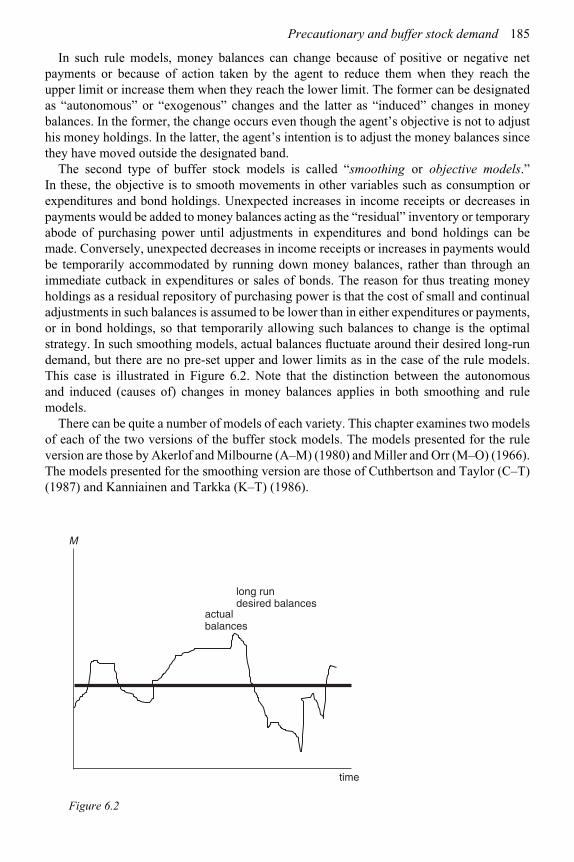
Precautionary and buffer stock demand 185
In such rule models, money balances can change because of positive or negative netpayments or because of action taken by the agent to reduce them when they reach theupper limit or increase them when they reach the lower limit. The former can be designatedas “autonomous” or “exogenous” changes and the latter as “induced” changes in moneybalances. In the former, the change occurs even though the agent’s objective is not to adjusthis money holdings. In the latter, the agent’s intention is to adjust the money balances sincethey have moved outside the designated band.
The second type of buffer stock models is called “smoothing or objective models.”In these, the objective is to smooth movements in other variables such as consumption orexpenditures and bond holdings. Unexpected increases in income receipts or decreases inpayments would be added to money balances acting as the “residual” inventory or temporaryabode of purchasing power until adjustments in expenditures and bond holdings can bemade. Conversely, unexpected decreases in income receipts or increases in payments wouldbe temporarily accommodated by running down money balances, rather than through animmediate cutback in expenditures or sales of bonds. The reason for thus treating moneyholdings as a residual repository of purchasing power is that the cost of small and continualadjustments in such balances is assumed to be lower than in either expenditures or payments,or in bond holdings, so that temporarily allowing such balances to change is the optimalstrategy. In such smoothing models, actual balances fluctuate around their desired long-rundemand, but there are no pre-set upper and lower limits as in the case of the rule models.This case is illustrated in Figure 6.2. Note that the distinction between the autonomousand induced (causes of) changes in money balances applies in both smoothing and rulemodels.
There can be quite a number of models of each variety. This chapter examines two modelsof each of the two versions of the buffer stock models. The models presented for the ruleversion are those by Akerlof and Milbourne (A–M) (1980) and Miller and Orr (M–O) (1966).The models presented for the smoothing version are those of Cuthbertson and Taylor (C–T)(1987) and Kanniainen and Tarkka (K–T) (1986).
long rundesired balances
M
time
actualbalances
Figure 6.2
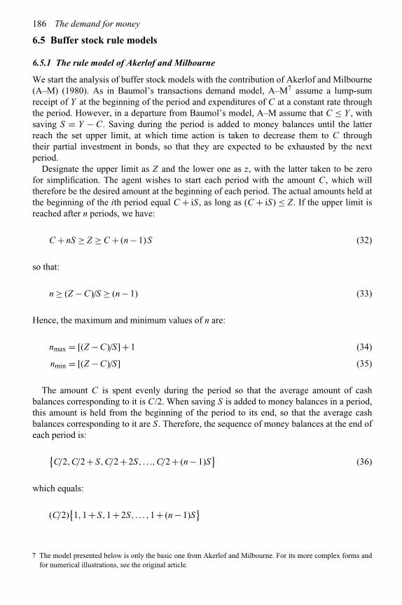
186 The demand for money
6.5 Buffer stock rule models
6.5.1 The rule model of Akerlof and Milbourne
We start the analysis of buffer stock models with the contribution of Akerlof and Milbourne(A–M) (1980). As in Baumol’s transactions demand model, A–M7 assume a lump-sumreceipt of Y at the beginning of the period and expenditures of C at a constant rate throughthe period. However, in a departure from Baumol’s model, A–M assume that C ≤ Y , withsaving S = Y − C. Saving during the period is added to money balances until the latterreach the set upper limit, at which time action is taken to decrease them to C throughtheir partial investment in bonds, so that they are expected to be exhausted by the nextperiod.
Designate the upper limit as Z and the lower one as z, with the latter taken to be zerofor simplification. The agent wishes to start each period with the amount C, which willtherefore be the desired amount at the beginning of each period. The actual amounts held atthe beginning of the ith period equal C + iS, as long as (C + iS) ≤ Z . If the upper limit isreached after n periods, we have:
C + nS ≥ Z ≥ C + (n − 1)S (32)
so that:
n ≥ (Z − C)/S ≥ (n − 1) (33)
Hence, the maximum and minimum values of n are:
nmax = [(Z − C)/S]+ 1 (34)
nmin = [(Z − C)/S] (35)
The amount C is spent evenly during the period so that the average amount of cashbalances corresponding to it is C/2. When saving S is added to money balances in a period,this amount is held from the beginning of the period to its end, so that the average cashbalances corresponding to it are S. Therefore, the sequence of money balances at the end ofeach period is:
{C/2,C/2 + S,C/2 + 2S, . . .,C/2 + (n − 1)S
}(36)
which equals:
(C/2){1,1 + S,1 + 2S, . . . ,1 + (n − 1)S
}
7 The model presented below is only the basic one from Akerlof and Milbourne. For its more complex forms andfor numerical illustrations, see the original article.

Precautionary and buffer stock demand 187
Let n be the number of periods before an induced transfer takes place. Then, over n periods,the average balance between induced adjustments is:
M d = 1
n
[C
2+(
C
2+ S
)+(
C
2+ 2S
)+·· ·+
{C
2+ (n − 1)S
}]
= C
2+ S(n − 1)
2(37)
Using (34) and (35) to eliminate n in (37) implies the minimum and maximum values ofmoney balances as:
Mmax = Z/2 (38)
Mmin = (Z − S)/2 (39)
Hence, the average of the money balances held as a buffer stock, designated as M b, is:
M b = (1/2)(Mmax + Mmin)
= Z/2 − S/4(40)
so that:
∂M b/∂Y ∼= −(1/4)(∂S/∂Y ) < 0 (41)
where ∂S/∂Y is the marginal propensity to save, which is positive. Hence, ∂M b/∂Y isnegative. This is a surprising result. Its intuitive explanation is that, as income rises, theupper threshold is reached more quickly, so that the interval before the money holdings arerun down by an induced adjustment is shortened. As a result, the richer agents review theirmoney and bond holdings more often than those with lower incomes, ceteris paribus, andwill hold less balances on average.8
However, since the limits z and Z were assumed to be exogenously specified in theabove model, the impact of increases in Y on them is not incorporated in (40). Transactionsdemand analysis implies that both of these limits would be positive functions of the level ofexpenditures.9 Therefore, the impact of a rise in income would have a positive and a negativecomponent, with the net impact being of indeterminate sign unless a fuller model werespecified. Another limitation of the above model is that it does not distinguish between theexpected increases in income and the unexpected ones. The (z, Z) concept is more appropriateto the latter than to the former.
Akerlof and Milbourne extended their preceding model to the case of the uncertainty ofnet payments by assuming that the agent buys and pays for durable goods at uncertain times,with p as the probability of making such a purchase. For this case, the A–M result, under their
8 This result does not hold if the upper limit X is defined relative to income Y as xY.9 If we follow the pattern of Baumol’s transactions analysis, suitably adapted to the present context, z and Z will
be non-linear functions of Y .

188 The demand for money
simplifying assumptions that include S = sY , where s is the constant average propensity tosave, was that:
M b ≈ Z/2 − s (1 + p)(Y/4) < 0 (42)
where p is the probability of payments (for a durable goods purchase). (42) implies that:
∂M b/∂Y = −(s/4)[1 + p + Yp′(Y )] (43)
where p′ = ∂p/∂Y . Assuming p′ to be positive – that is, the probability of buying durablegoods increases with income – (43) implies that the income elasticity of money balances isagain negative.
The A–M model was meant to encompass both the transactions and precautionary demands.The agent’s desire to finance an amount of transactions C out of income receipts Y createshis transactions demand, while the uncertainty of payments adds an additional precautionarydemand. However, this framework does not properly capture the transactions demand since itignores the dependence of (z, Z) on total expenditures and does not make a distinction betweenexpected and unexpected changes in income. Its implication of a negative income elasticity ofmoney demand must therefore be accepted as reflecting the influence of saving, and especiallyunexpected saving, on money demand, with consumption – and hence permanent income –being held constant. Some of the ideas behind these criticisms will become clearer from thetheoretical and empirical models presented below.
6.5.2 The rule model of Miller and Orr
Miller and Orr (M–O) (1966) assumed that net receipts – which would be net payments for anegative value – of x at any moment follow a random walk with a zero mean over each period(e.g. a “day”).10 Assume that in any time interval (e.g. an “hour”) equaling 1/t(t = 24), xis generated as a sequence of independent Bernoulli trials. The individual believes with asubjective probability of p that he will have net receipts of x during each time interval (hour)or net payments of x with a probability of (1−p), so that, over an hour, the probability of anincrease in money holdings by x is p and that of a decrease by x is (1 − p).
Cash holdings over a decision period of T periods will have a mean and standard deviationgiven by:
μT = Ttx (p − q) (44)
σ 2T = 4Ttpqx2 (45)
where:x = net receipts per hourμT = mean cash holdings over T periodsσT = standard deviation of cash holdings over T periodsp = probability of positive net paymentsq = probability of negative net payments (= 1 − p)t = number of sub-intervals (hours) in each period (day)T = number of time periods up to the planning horizon.
10 Under this assumption, the pattern of net payments will possess stationarity and serial independence.

Precautionary and buffer stock demand 189
For simplification, p was assumed by M–O to be 1/2,11 so that:
μT = 0 (46)
σ 2T = Ttx2 (47)
Since the variance of changes in cash holdings (σ 2T ) during T periods is Ttx2, the variance
σ 2 of daily changes in balances (over the day) is:
σ 2 = σ 2T/T = tx2 (48)
The cost of holding and varying cash has two components: the interest cost of holding cashrather than bonds, and the brokerage cost of making deliberate changes in cash holdings. Theper period (daily) expected cost is:
E(TC) = B0E(N )/T + RM (49)
where:E(TC) = expected cost per period of holding and managing cashM = average daily cash balanceE(N ) = expected number of transactions between money and bonds over T periodsB0 = brokerage cost per transactionR = interest rate per period (day) on bonds.
The firm is taken to minimize (49) with respect to the upper limit Z and the lower limit zon cash balances. M–O show that under certain specific assumptions:
E(N )/T → 1/D (z,Z)
where D is the mean of the time intervals separating portfolio transfers between bonds andcash, and that:
D (z,Z) = z (Z − z)/tx2 (50)
Further, M–O show that the steady–state distribution of money balances during the day hasa discrete triangular distribution for p = 1/2, so that the average balances M are given by:
M = (Z + z)/3 (51)
Hence, using the maximum value of E(N )/T , (51) can be restated as:
E(TC) = B0 tx2/zw + R (w + 2z)/3 (52)
where w = Z − z. w is thus the width of the band. Setting the partial derivatives of (52) withrespect to z (with w constant), and w (with z constant) equal to zero, yields:
∂E(TC)/∂z = B0 tx2/z2w + 2r/3 = 0 (53)
∂E(TC)/∂w = −B0 tx2/zw2 + R/3 = 0 (54)
11 In this case, cash holdings follow a random walk without drift.
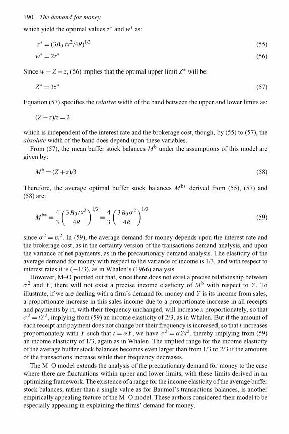
190 The demand for money
which yield the optimal values z∗ and w∗ as:
z∗ = (3B0 tx2/4R)1/3 (55)
w∗ = 2z∗ (56)
Since w = Z − z, (56) implies that the optimal upper limit Z∗ will be:
Z∗ = 3z∗ (57)
Equation (57) specifies the relative width of the band between the upper and lower limits as:
(Z − z)/z = 2
which is independent of the interest rate and the brokerage cost, though, by (55) to (57), theabsolute width of the band does depend upon these variables.
From (57), the mean buffer stock balances M b under the assumptions of this model aregiven by:
M b = (Z + z)/3 (58)
Therefore, the average optimal buffer stock balances M b∗ derived from (55), (57) and(58) are:
M b∗ = 4
3
(3B0 t x2
4R
)1/3
= 4
3
(3B0 σ 2
4R
)1/3
(59)
since σ 2 = tx2. In (59), the average demand for money depends upon the interest rate andthe brokerage cost, as in the certainty version of the transactions demand analysis, and uponthe variance of net payments, as in the precautionary demand analysis. The elasticity of theaverage demand for money with respect to the variance of income is 1/3, and with respect tointerest rates it is (−1/3), as in Whalen’s (1966) analysis.
However, M–O pointed out that, since there does not exist a precise relationship betweenσ 2 and Y , there will not exist a precise income elasticity of M b with respect to Y . Toillustrate, if we are dealing with a firm’s demand for money and Y is its income from sales,a proportionate increase in this sales income due to a proportionate increase in all receiptsand payments by it, with their frequency unchanged, will increase x proportionately, so thatσ 2 = tY 2, implying from (59) an income elasticity of 2/3, as in Whalen. But if the amount ofeach receipt and payment does not change but their frequency is increased, so that t increasesproportionately with Y such that t = αY , we have σ 2 = αYx2, thereby implying from (59)an income elasticity of 1/3, again as in Whalen. The implied range for the income elasticityof the average buffer stock balances becomes even larger than from 1/3 to 2/3 if the amountsof the transactions increase while their frequency decreases.
The M–O model extends the analysis of the precautionary demand for money to the casewhere there are fluctuations within upper and lower limits, with these limits derived in anoptimizing framework. The existence of a range for the income elasticity of the average bufferstock balances, rather than a single value as for Baumol’s transactions balances, is anotherempirically appealing feature of the M–O model. These authors considered their model to beespecially appealing in explaining the firms’ demand for money.

Precautionary and buffer stock demand 191
6.6 Buffer stock smoothing or objective models
6.6.1 The smoothing model of Cuthbertson and Taylor
The basic partial adjustment model (PAM), in the context of a single period, often assumesthat the adjustment in money balances involves two kinds of costs. One of these is the costof deviations of actual balances from their desired amount. The second element is the costof changing the current level of balances from their amount in the preceding period. Theone-period first-order PAM12 assumes that the cost function is quadratic in its two elements,as in:
TC = a (Mt − M ∗t )2 + b (Mt − Mt−1)2 (60)
where:TC = present discounted value of the total cost of adjusting balancesM = actual money balancesM ∗ = desired money balances.
The buffer stock models (Carr and Darby, 1981; Cuthbertson, 1985; Cuthbertson andTaylor, 1987; and others) posit an intertemporal cost function rather than a one-period oneand minimize the present expected value of this cost over the present and future periods.This implies taking account of both types of costs over the present as well as the futureperiods. Hence, for the first element of cost, the expected cost of future deviations of actualfrom desired balances, in addition to the cost of a current deviation, is taken into account.This modification allows the agent to take account of the future levels of desired balances indetermining the present amounts held. For the second element of cost, the justification forthe intertemporal extension is as follows: just as last period’s money holdings affect the costof adjusting this period’s money balances, so would this period’s balances affect the cost ofadjusting next period’s balances, and so on, and these future costs attached to current moneybalances need to be taken into consideration in the current period. The resulting cost functionis intertemporal and forward looking.
The intertemporal extension of (60) for i = 0,1, . . .,T is:
TC = �iDi[a(Mt+i − M ∗
t+i)2 + b(Mt+i − Mt+i−1)2
](61)
where:
D = gross discount rate (= 1/(1 + r)).
In equation (61), a is the cost of actual balances being different from desired balances andb is the cost of adjusting balances between periods. b can be the brokerage cost of sellingbonds but, as we have seen in earlier discussions, this can be more than just a monetary cost.The economic agent is assumed to minimize TC with respect to Mt+i, i = 0,1, . . . ,T . ItsEuler condition for the last period T is:
∂TC/∂Mt+T = 2a(Mt+T − M ∗t+T ) + 2b(Mt+T − Mt+T−1) = 0
12 See Chapter 7 for the treatment of one-period partial adjustment models in the context of money demandfunctions.
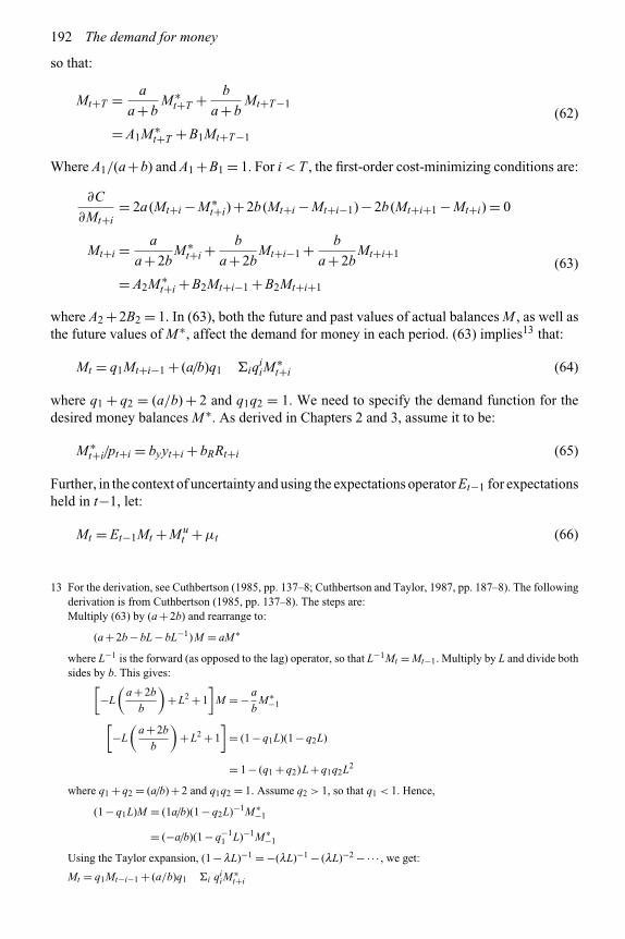
192 The demand for money
so that:
Mt+T = a
a + bM ∗
t+T + b
a + bMt+T−1
= A1M ∗t+T + B1Mt+T−1
(62)
Where A1/(a+b) and A1 +B1 = 1. For i < T , the first-order cost-minimizing conditions are:
∂C
∂Mt+i= 2a (Mt+i − M ∗
t+i) + 2b (Mt+i − Mt+i−1) − 2b (Mt+i+1 − Mt+i) = 0
Mt+i = a
a + 2bM ∗
t+i +b
a + 2bMt+i−1 + b
a + 2bMt+i+1
= A2M ∗t+i + B2Mt+i−1 + B2Mt+i+1
(63)
where A2 +2B2 = 1. In (63), both the future and past values of actual balances M , as well asthe future values of M ∗, affect the demand for money in each period. (63) implies13 that:
Mt = q1Mt+i−1 + (a/b)q1 �iqiiM
∗t+i (64)
where q1 + q2 = (a/b) + 2 and q1q2 = 1. We need to specify the demand function for thedesired money balances M ∗. As derived in Chapters 2 and 3, assume it to be:
M ∗t+i/pt+i = byyt+i + bRRt+i (65)
Further, in the context of uncertainty and using the expectations operator Et−1 for expectationsheld in t−1, let:
Mt = Et−1Mt + Mut +μt (66)
13 For the derivation, see Cuthbertson (1985, pp. 137–8; Cuthbertson and Taylor, 1987, pp. 187–8). The followingderivation is from Cuthbertson (1985, pp. 137–8). The steps are:Multiply (63) by (a + 2b) and rearrange to:
(a + 2b − bL − bL−1)M = aM ∗
where L−1 is the forward (as opposed to the lag) operator, so that L−1Mt = Mt−1. Multiply by L and divide bothsides by b. This gives:[
−L
(a + 2b
b
)+ L2 + 1
]M = − a
bM ∗−1
[−L
(a + 2b
b
)+ L2 + 1
]= (1 − q1L)(1 − q2L)
= 1 − (q1 + q2)L + q1q2L2
where q1 + q2 = (a/b) + 2 and q1q2 = 1. Assume q2 > 1, so that q1 < 1. Hence,
(1 − q1L)M = (1a/b)(1 − q2L)−1M ∗−1
= (−a/b)(1 − q−11 L)−1M ∗−1
Using the Taylor expansion, (1 − lL)−1 = −(lL)−1 − (lL)−2 −·· · , we get:
Mt = q1Mt−i−1 + (a/b)q1 �i qiiM
∗t+i

Precautionary and buffer stock demand 193
where M ut has been introduced to take account of errors in the expected value of M ∗
t+i due tounexpected changes in its determinants in (65). From (64) to (66),
Mt = q1Mt−1 + (a/b)q1�i qii
{byyt+i + bRRt+i
}pt + M u
t +μt (67)
In (67), the actual demand for money depends upon the future and current values of incomeand interest rates, which shows the model to be a forward-looking one. It also depends uponthe lagged value of money balances, thus incorporating a backward-looking element. Themodel is, therefore, both forward and backward looking. Note that the estimation of (67)will require the prior specification of the mechanism for deriving the expected future valuesof y and R, and also of the mechanism for the estimation of M u. The estimation proceduresfor these are discussed in Chapter 7.
6.6.2 The Kanniainen and Tarkka (1986) smoothing model
An alternative version of the intertemporal adjustment cost function (61), used by Kanniainenand Tarkka (K–T) (1986),14 is:
TC = Et�i[Di{a(Mt+i − M ∗
t+i)2 + b (zt+i)
2}] i = 0,1,2, . . . (68)
where zt are the “induced” changes in money balances brought about by the agent’s ownactions and b is interpreted as the brokerage cost of converting bonds to money. The othervariables are as defined earlier, with M being nominal balances, M ∗ the steady-state desiredbalances and D the discount factor. The rationale for this specification of the cost function isthat while the induced changes in money holdings impose a brokerage cost, the autonomouschanges do not since they result from the actions of others. The adjustment in nominalbalances in t from those in t−1 occurs due to autonomous and induced changes in t, so that:
Mt − Mt−1 = zt + xt (69)
where:zt = induced changes in money holdingsxt = autonomous changes.
Substitute (69) in (68) and, to minimize total cost, set the first-order partial derivatives ofthe resulting equation with respect to mt+i, i = 0,1,2, . . ., equal to zero. This process yieldsthe Euler equations as:
EtMt+i+1 −βEtMt+i + (1 + R)EtMt+i−1 = −αEtM∗t+i + Etxt+i+1 − (1 + R)Etxt+i
(70)
where:α = a/Dbβ = (1/D)
{(a/b) + D + 1
}i = 0,1,2, . . . .
Note that (70) represents a large number of equations and shows the extensive informationrequirements of such models. To determine money demand in period t, the agent must have
14 The following exposition is based on Kanniainen and Tarkka (1986) and Mizen (1994, pp. 50–51).

194 The demand for money
expectations on the autonomous changes in money holdings in (t +1) and its optimal moneybalances, with the latter requiring this information for period (t + 2), and so on. With newinformation becoming available each period, the model will require continual recalculation.
Equation (70) is a stochastic second-order difference equation in Et Mt+i. Its roots are:
l1,l2 = (1/2)[β ± {β2 − 4(1 + R)
}1/2]
with l1 > 0 being the stable root and l2 < 0 being the unstable one. The latter was ignored byK–T in order to exclude cyclical adjustment. Using the positive root l1, the Euler conditionbecomes:
EtMt+1 = l1Mt +[l1α/(1 + R − l1)
]M ∗
t −�i[l1/(1 + R)
]i[Etxt+i−1 − (1 + R)Etxt+i
](71)
In (71), the impact of the autonomous adjustment xt on money demand is given by l1, thestable root of (70). This impact is the same whether it was anticipated or not.15 The impact offuture autonomous shocks, on which expectations have to be formed, depends upon the rateof time preference. If this rate is high, these expectations will have to be formed for only someperiods ahead. Further, changes in these expectations will shift the money demand function.
Substitute (71) into (70) and solve for Mt , noting that EtM ∗t = M ∗
t . This yields:
Mt = l1Mt−1 +ρM ∗t + l1xt + zt (72)
where ρ = [l1(a/b)(1 + R)/
(1 + R − l1)] and z∗t represents the weighted sum of the future
shocks to net receipts and payments. z∗t is given by:
z∗t = −(1 − l1)�i
{l1/(1 + R)
}iEtxt+j (73)
The above model can be transformed into real terms by dividing (71) by the current pricelevel pt . The resulting equation, based on (71),16 is:
ln mt = a0 + (1 − l1)ln m∗t + l1ln mt−1 + γ ln pt/pt−1 + l1xt/Mt−1 + zt/Mt−1 (74)
where mt = Mt/Pt and m∗t = M ∗
t /Pt .
15 This conclusion differs from that of Carr and Darby (1981) and Santomero and Seater (1981).16 The procedure is as follows. Subtracting Mt−1 from both sides of (72) gives:
Mt − Mt−1 = (1 − l1)[ρ/(1 − l1)M ∗
t − Mt−1]+ l1xt + zt
Divide both sides of this equation by Mt−1 and use the approximation ln (1+n) ∼= n for small values of n. Thisgives:
In Mt = ln[ρ/(1 − l1)
]1−l1 + (1 − l1)ln M ∗t + l1Mt−1 + l1xt/Mt−1 + zt/Mt−1
Now subtract ln pt from both sides and also add and subtract the term l1 ln pt−1. This will give (74) with
a0 = ln[ρ/(1 − l1)
]1−l1 . See K–T for the derivations of these equations and those reported in the text.
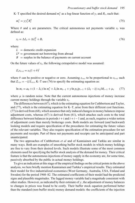
Precautionary and buffer stock demand 195
K–T specified the desired demand m∗t as a log-linear function of yt and Rt , such that:
m∗t = γ yθ
t Rηt (75)
Where θ and η are parameters. The critical autonomous net payments variable xt wasdefined as:
xt = �Lt +�Lgt + Bt (76)
where:L = domestic credit expansionLg = government net borrowing from abroadB = surplus in the balance of payments on current account
On the future values of xt , the following extrapolative model was assumed:
Etxt+i = xt(1 + θ )i
where θ can be positive or negative or zero. Assuming zt+i to be proportional to xt+i suchthat Zt+i = −ξXt+i, K–T use (74) to specify the estimating equation as:
ln mt = a0 + (1 − l1) ln m∗t + l1ln mt−1 + γ ln pt/pt−1 + (l1 − ξ ) xt/Mt−1 +μt (77)
where μ is random noise. Note that the current autonomous injections of money increasecurrent money holdings through the variable xt .
The differences between (67), which is the estimating equation for Cuthbertson and Taylor,and (77), which is the estimating equation for K–T, arise from their different cost functions.(77) is derived from (68), which assumes that only induced changes in money balances imposeadjustment costs, whereas (67) is derived from (61), which attaches such costs to the totaldifference between balances in periods t + i and t + i−1 and, as such, requires a wider notionof adjustment costs than merely brokerage costs. Both models are forward (and backward)looking models and require specification of the procedures for estimating the future valuesof the relevant variables. They also require specification of the estimation procedure for netpayments and receipts. Part of these net payments and receipts can be anticipated and partunanticipated.
The two approaches of Cuthbertson et al and of Kanniainen and Tarkka are similar inmany ways. Both are examples of smoothing buffer stock models in which money holdingsare free to vary from their desired levels. Such models illustrate some of the most commonelements used for specifying the buffer stock analysis of the demand for money. Their criticalfeature is that the autonomous injections of money supply in the economy are, for some time,passively absorbed by the public in actual money holdings.
To give an indication at this stage of the empirical findings on the critical points in the aboveanalysis, we here briefly mention Kanniainen and Tarkka’s empirical results. They estimatedtheir model for five industrialized economies (West Germany, Australia, USA, Finland andSweden) for the period 1960–82. The estimated coefficients of their model had the predictedsigns and plausible magnitudes. The lagged money variable had a magnitude consistent withother studies. However, as indicated by their estimate of γ , the adjustment of money balancesto changes in prices was found to be costly. Their buffer stock equation performed betterthan the standard (non-buffer stock) money demand models: the coefficients of the injection
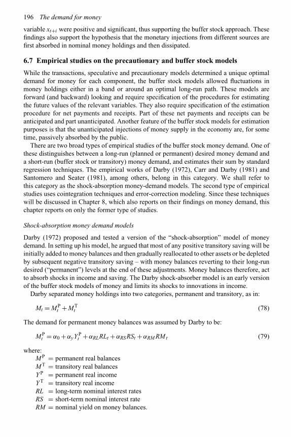
196 The demand for money
variable xt+i were positive and significant, thus supporting the buffer stock approach. Thesefindings also support the hypothesis that the monetary injections from different sources arefirst absorbed in nominal money holdings and then dissipated.
6.7 Empirical studies on the precautionary and buffer stock models
While the transactions, speculative and precautionary models determined a unique optimaldemand for money for each component, the buffer stock models allowed fluctuations inmoney holdings either in a band or around an optimal long-run path. These models areforward (and backward) looking and require specification of the procedures for estimatingthe future values of the relevant variables. They also require specification of the estimationprocedure for net payments and receipts. Part of these net payments and receipts can beanticipated and part unanticipated. Another feature of the buffer stock models for estimationpurposes is that the unanticipated injections of money supply in the economy are, for sometime, passively absorbed by the public.
There are two broad types of empirical studies of the buffer stock money demand. One ofthese distinguishes between a long-run (planned or permanent) desired money demand anda short-run (buffer stock or transitory) money demand, and estimates their sum by standardregression techniques. The empirical works of Darby (1972), Carr and Darby (1981) andSantomero and Seater (1981), among others, belong in this category. We shall refer tothis category as the shock-absorption money-demand models. The second type of empiricalstudies uses cointegration techniques and error-correction modeling. Since these techniqueswill be discussed in Chapter 8, which also reports on their findings on money demand, thischapter reports on only the former type of studies.
Shock-absorption money demand models
Darby (1972) proposed and tested a version of the “shock-absorption” model of moneydemand. In setting up his model, he argued that most of any positive transitory saving will beinitially added to money balances and then gradually reallocated to other assets or be depletedby subsequent negative transitory saving – with money balances reverting to their long-rundesired (“permanent”) levels at the end of these adjustments. Money balances therefore, actto absorb shocks in income and saving. The Darby shock-absorber model is an early versionof the buffer stock models of money and limits its shocks to innovations in income.
Darby separated money holdings into two categories, permanent and transitory, as in:
Mt = MPt + MT
t (78)
The demand for permanent money balances was assumed by Darby to be:
MPt = α0 +αyY P
t +αRLRLt +αRSRSt +αRM RMt (79)
where:MP = permanent real balancesMT = transitory real balancesY P = permanent real incomeY T = transitory real incomeRL = long-term nominal interest ratesRS = short-term nominal interest rateRM = nominal yield on money balances.

Precautionary and buffer stock demand 197
Equation (79) specifies the dependence of permanent balances on permanent income andvarious interest rates.
For transitory balances MT, Darby assumed that:
�MTt = β1ST
t +β2MTt−1 0 > β1 > 0, β2 < 0 (80)
where the proportion β1 of transitory real saving ST is added to transitory real balances duringthe period, but last period’s transitory balances are run down or adjusted at the rate β2.
Darby used Milton Friedman’s ideas on permanent and transitory income in which:
Yt = Y Pt + Y T
t (81)
where permanent and transitory income are not correlated with each other and permanentincome is generated by an adaptive expectations procedure. Further,
STt = Y T
t − CTt (82)
where transitory consumption CT is an independent random variable with a zero mean, so thatY T
t was substituted for STt in the estimating equation. As mentioned above, a proportion β1 of
it is accumulated in transitory money balances during the period and eventually reallocatedto other assets.
Equations (78) to (82) imply that:
Mt = α0 (1 −β) +β1Y Tt +βMt−1 +αY Y P∗
t +αRLRL∗t +αRSRS∗
t +αRM RM ∗t (83)
where β = (1 + β2), Y P∗ = (1 − β)Y Pt , RL∗
t = (1 − β)RLt, RS∗t = (1 − β)RSt and
RM ∗t = (1 −β)RMt .
Darby’s finding for USA for the period 1947:1 to 1966:4 was that β1 was about 40 percent,so that transitory income and saving had a strong effect on money balances and transitorybalances increased by about 40 percent of transitory income. β2, the induced reduction intransitory balances per quarter, was about 20 percent. These findings support the bufferstock approach where net income receipts are temporarily added to money balances and thengradually adjusted at periodic intervals. The estimated adjustment is relatively slow, thoughDarby also found that both β1 and β2 had increased since the 1940s. With the increasinginnovation in the financial markets in recent decades, the increase is likely to have continuedand be quite significant.
While the above model introduces the notion of transitory money balances arising fromtransitory income and saving into the analysis, it does not deal with the differing effects ofanticipated and unanticipated changes in the money supply, and therefore does not deal withinnovations in money supply. Carr and Darby (1981) argue that the anticipated changes inmoney supply are integrated by economic agents into their decisions on consumption, etc. andare therefore already incorporated into the current price level, with real balances held beingunaffected by the changes in the price level and the anticipated money changes. However,the unanticipated money supply change alters the net receipts of the public and can be treatedas an element of transitory income. It may be wholly or partly added to buffer balances, isthereby not spent and is not reflected in the price level. Hence, changes in the unanticipatedmoney supply alter real balances while changes in the anticipated money supply do not.

198 The demand for money
To incorporate these arguments into the analysis, Carr and Darby (1981) assumed that:
M st = M s∗
t + M sut (84)
where:M s = nominal money supplyM s∗ = anticipated nominal money supplyM su = M s − M s∗ = unanticipated nominal money supply.
The short-run desired demand function was specified in real terms, with a partial adjustmentmodel, as:
mdt − mt−1 = l (m∗
t − mt−1) (85)
where:md = short-run desired demand for real balances (log scale)m* = long-run desired demand for real balances (log scale)
so that the desired short-run demand for real balances is:
mdt = lm∗
t + (1 − l)mt−1 (86)
where the short-run desired demand for real balances is a weighted average of the long-rundemand and one-period lagged balances. The actual holdings of money balances are the sumof the short-run desired balances, transitory income and unanticipated money supply. Hence:
mt = lm∗t + (1 − l)mt−1 +βyT
t + bM sut (87)
The long-run desired demand is given by:
m∗t = γ0 + γ1yP
t + γ2Rt (88)
Therefore:
mt = lγ0 + lγ1yPt + lγ2Rt + (1 − l)mt−1 +βyT
t + bM sut (89)
Permanent and transitory income were measured as in the Darby model earlier; incalculating permanent income, the weight on the current quarterly income was set at0.025 percent. In the present model, the demand for real balances depends upon transitoryincome and unanticipated money supply changes. The theoretical arguments require theircoefficients to be positive.
Carr and Darby (1981) tested this model for eight industrial countries (USA, UK, Canada,France, Germany, Italy, Japan and the Netherlands) for the period 1957:1 to 1976:4 andreported that the coefficient b on unanticipated money supply was significant and rangedbetween 0.7 and 1 for all countries, using generalized least-squares (GLS) estimates. Thecoefficient β was significant and positive for the USA but was not significant for the othercountries. To illustrate, using GLS estimates for the coefficients, the estimated value of β (thecoefficient for transitory income) was 0.090 while that of b (the coefficient for unanticipatedmoney supply) was 0.803 for the USA; the corresponding estimate of β for Canada was0.018, which was not significant, but the estimate of b was 0.922 which was significant.Hence, the influence of transitory income on money balances was much weaker than that
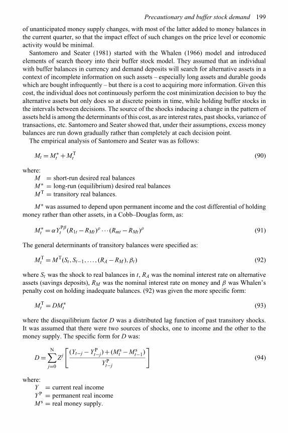
Precautionary and buffer stock demand 199
of unanticipated money supply changes, with most of the latter added to money balances inthe current quarter, so that the impact effect of such changes on the price level or economicactivity would be minimal.
Santomero and Seater (1981) started with the Whalen (1966) model and introducedelements of search theory into their buffer stock model. They assumed that an individualwith buffer balances in currency and demand deposits will search for alternative assets in acontext of incomplete information on such assets – especially long assets and durable goodswhich are bought infrequently – but there is a cost to acquiring more information. Given thiscost, the individual does not continuously perform the cost minimization decision to buy thealternative assets but only does so at discrete points in time, while holding buffer stocks inthe intervals between decisions. The source of the shocks inducing a change in the pattern ofassets held is among the determinants of this cost, as are interest rates, past shocks, variance oftransactions, etc. Santomero and Seater showed that, under their assumptions, excess moneybalances are run down gradually rather than completely at each decision point.
The empirical analysis of Santomero and Seater was as follows:
Mt = M ∗t + MT
t (90)
where:M = short-run desired real balancesM ∗ = long-run (equilibrium) desired real balancesMT = transitory real balances.
M ∗ was assumed to depend upon permanent income and the cost differential of holdingmoney rather than other assets, in a Cobb–Douglas form, as:
M ∗t = αY Pβ
t (R1t − RMt)ρ · · · (Rmt − RMt)
ρ (91)
The general determinants of transitory balances were specified as:
MTt = MT(St,St−1, . . . , (RA − RM ),βt) (92)
where St was the shock to real balances in t, RA was the nominal interest rate on alternativeassets (savings deposits), RM was the nominal interest rate on money and β was Whalen’spenalty cost on holding inadequate balances. (92) was given the more specific form:
MTt = DM ∗
t (93)
where the disequilibrium factor D was a distributed lag function of past transitory shocks.It was assumed that there were two sources of shocks, one to income and the other to themoney supply. The specific form for D was:
D =N∑
j=0
Zj
[(Yt−j − Y P
t−j) + (M st − M s
t−1)
Y Pt−j
](94)
where:Y = current real incomeY P = permanent real incomeM s = real money supply.

200 The demand for money
Equation (94) assumes that all shocks, whether from income or money supply changes,have the same pattern of effects on transitory balances. Further, innovations in money demandare not considered, so that either they do not occur17 or real balances adjust instantly to them.If the money demand function is unstable, (94) should be modified to include shifts in moneydemand.
The estimated demand function for short-run balances implied by (90) to (94) is of theform:
M dt = αY
Pβt (R1t −RMt )γ · · · (Rmt −RMt )ρ
×⎡⎣1 +
N∑j=0
Zj
((Yt−j −Y P
t−j) + (M st −M s
t−1
Y Pt−j
)⎤⎦
δ
(95)
where α,β,δ > 0 and γ,ρ < 0, and Ri is the nominal rate of return on the ith asset.The above model was estimated for M1 and M2 for the USA for the period 1952:2 to
1972:4, using the Cochrane–Orcutt technique to eliminate first-order serial correlation. Itwas assumed in the estimation process that equilibrium was achieved within each quarterbetween the money supply and the short-run money demand, so that the latter was proxied bythe money supply. Only two interest rates – the commercial paper rate and the commercialpassbook rate – were used. The estimate of the coefficient Z was significant and positivefor both M1 and M2. Hence, both transitory income and changes in the money supply had ashort-run positive impact on short-run money demand, thereby showing evidence of bufferholdings of money balances. Further, transitory balances did not increase proportionatelywith the magnitude of the shock, so that large shocks were corrected faster than smaller ones.M1 and M2 holdings adjusted within two to three quarters to their desired levels, implyinga fairly fast rate of adjustment.
A microfoundations search model of precautionary balances
Faig and Jerez (2007) use microeconomic optimizing foundations to model the demand formoney as a demand for precautionary balances held against uncertain expenditure needs.They build a search model incorporating shocks to individuals’ preferences. Individualsdecide on their money balances prior to the unknown preference shock, with large preferenceshocks assumed to be rarer than small ones. At low interest rates, individuals hold enoughbalances so that their consumption purchases are not very liquidity constrained, but theyare willing to allow their purchases to be liquidity constrained to a greater extent at higherinterest rates, so that velocity falls at higher interest rates. Their empirical estimates forthe USA for the periods 1892 to 2004 capture the fall in the velocity of M1 during thelow-interest period of the Great Depression and its rise from the mid-1960s to the mid-1980s, which had high interest rates. Financial innovations, such as credit cards, Internetbanking, etc., as well as the reduction in brokerage costs (which has reduced the cost oftransfers between M1 and other assets), have meant that households can better accommodateunexpected expenditures, even with inadequate money balances. These developments have
17 Santomero and Seater (1981) assume that the money demand function is stable. In fact, empirical studies inrecent decades have shown it to be unstable and therefore to generate transitory excess money holdings.

Precautionary and buffer stock demand 201
reduced the need for precautionary balances. Therefore, the empirical impact of financialinnovations and the IT revolution has been to reduce the demand for M1 and increase itsvelocity.
Conclusions
This chapter has presented some of the basic models of the precautionary demand for money.This demand arises because of the uncertainty of the timing of payments and receipts, so that amajor determinant of such demand is the probability distribution of net payments. Whalen’sanalysis captured this by the variance of the distribution, under the assumptions that thedistribution was normal and the individual wanted to keep balances equal to a specifiedproportion of the variance of the distribution. How much of this proportion is kept by aparticular individual will depend upon his degree of risk aversion. This analysis shows thatthe elasticities of precautionary demand with respect to interest rates and income are not 1/2,as were the elasticities for transactions demand under certainty of the timing of receipts andpayments, but are likely to be lower.
The precautionary demand analysis also brings the interest rates on stand-by credit facilitiessuch as overdrafts and trade credit, and the penalties for being caught short of a paymentmedium, into the determinants of the precautionary demand and through it into those of thetotal demand for money. Such facilities and penalties differ between households and firms,and between large and small firms. Further, they often also differ by industry, so that weshould expect the demand functions for money to differ between sectors and industries.
Is the precautionary demand for money a significant part of the total money balances?The answer to this will depend upon the degree of uncertainty of income and expenditures,and the relative penalty costs of being caught short of funds. Some numerical calculationsdone by Sprenkle and Miller suggest that the precautionary balances can be about one-thirdor more of the transactions balances. Further, with the increasing availability of short-termassets, which offer a higher return without a significantly higher risk than M1, the speculativedemand for M1 would nowadays be insignificant, so that the precautionary demand could begreater than the speculative demand. Consequently, the study of the precautionary demandfor money has become more prominent in recent years. On the negative side, the increasingavailability of several close substitutes for M1 means that the precautionary needs of theindividual could also be met by the holdings of such near-monies, so that the precautionarydemand for M1 would also be small.
Since the precautionary demand for money reflects the influence of the uncertainty ofincomes and expenditures, fluctuations in this degree of uncertainty over the business cyclewould imply fluctuations in the precautionary balances over the cycle. Boom periods of highemployment and low uncertainty of income would mean a lower precautionary demand formoney, for given income levels, than recessionary periods with greater uncertainty of keepingone’s job. A higher variance of the rate of inflation would imply a higher variance of netreceipts and therefore a higher precautionary demand for money. Provision of national healthcare (medicare) under which no payment has to be rendered for medical services reducesboth precautionary savings and precautionary money demand.
The buffer stock approach constitutes a very significant innovation in money demandmodeling and represents an extension of the notions behind the precautionary demand formoney. However, this approach goes further than the pure precautionary demand motive byrecognizing that there are different costs of adjusting various types of flows and stocks, andthat, for the individual, adjustment in money balances is often the least cost immediate option

202 The demand for money
for many types of shocks. The result is that money balances are increased and decreased as abuffer in response to many types of shocks, and are only adjusted to their long-run equilibriumlevels as and when it becomes profitable to adjust other stocks and flows. Hence, a distinctionhas to be drawn not only between short-run desired money balances and long-run ones,but also between the former and the balances actually being held. The difference betweenthese concepts is buffer stock balances. Actual balances will be larger than short-run desiredbalances for positive (unanticipated) shocks to the money supply and to income, and smallerfor negative shocks in the latter. Hence, unlike the standard money-demand models, thebuffer-stock models imply the dependence of money demand on the shocks to money supply,so that short-run money demand is not independent of money-supply shifts.
The divergence of actual balances from the short-run desired balances and of the latter fromthe long-run balances provides one explanation for the delayed response of nominal incomeand interest rates to monetary policy where the latter include unanticipated changes in moneysupply. Hence, in terms of the implications of the buffer-stock models for monetary policy,these models imply that since part of the changes in the money supply are accommodatedthrough passive money holdings, the impact of such changes on market interest rates iscorrespondingly smaller and the full impact takes some time to occur. Correspondingly, thefull impact of such money supply changes on nominal national income takes several periodsand is larger than the short-term effect.
While the rule models, with money balances fluctuating in a band with upper and lowerlimits, inaugurated the buffer stock notion through the pioneering contribution of Miller andOrr (1966), empirical work has tended to follow the ideas of the smoothing models.
The empirical work of Carr and Darby (1981) provides comparison between the relativeeffects of income shocks and money-supply shocks. The effect of the income shocks on moneydemand is weaker and, for many countries, insignificant while the effect of the money-supplyshocks is significant and substantially stronger. The latter represents a confirmation of thebuffer stock hypothesis.
These findings imply that – since some part of the changes in the money supply result inpassive money holdings, which are then gradually eliminated over time – the impact of suchmoney supply changes on market interest rates is correspondingly smaller and the full impacttakes some time to occur. This has been confirmed in the findings, reported in Chapter 9,from many error-correction models. Further, the full impact of money supply changes onnominal national income will also take several quarters and the overall effect will be largerthan the short-term one.
Summary of critical conclusions
❖ Precautionary savings and precautionary money demand arise because of the uncertaintyof either income or expenditures.
❖ Precautionary money demand depends on the variances of income and expenditures andthe availability of overdraft facilities, as well as on the penalty cost of a shortfall in moneyholdings.
❖ Buffer stock money demand arises because money has a lower cost of adjustment thancommodities, labor and leisure. Money acts as a passive short-term inventory of purchasingpower until it is optimal to make adjustments in the latter set of variables.
❖ Rule models of buffer stock money demand allow fluctuations in money demand in a rangebetween pre-selected upper and lower limits.

Precautionary and buffer stock demand 203
❖ Smoothing models of buffer stock money demand imply that actual money holdings willvary around their desired long-run level.
❖ Precautionary and buffer stock holdings of money would vary with the phase, duration andamplitude of the business cycle, and with unemployment rate.
❖ Precautionary and buffer stock holdings of money also depend on the availability of otherhighly liquid interest-bearing assets in the economy. In the presence of these, such holdingscould be insignificant.
❖ Empirical evidence confirms the existence of buffer stock holdings of money balances.Therefore, money demand is not independent of money supply.
Review and discussion questions
1. “Individuals hold money because of uncertainty over the timing of transactions.Therefore, the theory of the transactions demand for money must take account of thisuncertainty.” Discuss this statement.
How can this uncertainty be incorporated into a model utilizing the inventory analysisof the transactions demand for money? Present a model that does so.
2. What is the buffer stock demand for money and how does it differ from the precautionarymoney demand? Present at least one model of each that shows such a difference.
3. If the speculative demand for money is zero in a financially developed economy, assome have claimed, is the precautionary demand for money also zero? Evaluate withreference to both M1, M2 and broader monetary aggregates. If both the speculativeand precautionary components of money demand are zero, what about the transactionsdemand? Consider both households and firms in your answer.
4. “Some recent empirical studies seem to show that the money demand function may notbe independent of the money supply function.” Report on the methodology and resultsof at least one such study.
5. If money demand is dependent on changes in the money supply in the short-run, asthe buffer stock models show, does the functional form of the money demand functionremain the same or change? What are the arguments of the money demand functionincorporating a buffer stock component? How would you estimate this function?
6. What is the justification for and what are the arguments against the buffer stockapproaches to money demand?
7. To what extent is Baumol’s inventory-theoretic approach, with its assumption ofcertainty, a satisfactory explanation of money demand?
How does managing an inventory of money differ from managing inventories ofgoods? How do such differences affect the speed of adjustment of money demand toexpected and unexpected changes in money supply?
8. Present at least one rule model and one smoothing model of the buffer stock demand formoney. What are the major differences in their implied money demand functions?
References
Akerlof, G.A., and Milbourne, R.D. “The short-run demand for money.” Economic Journal, 90, 1980,pp. 885–900.
Carr, J., and Darby, M.R. “The role of money supply shocks in the short-run demand for money.”Journal of Monetary Economics, 8, 1981, pp. 183–99.

204 The demand for money
Cuthbertson, K. The Supply and Demand for Money. Oxford: Basil Blackwell, 1985, pp. 30–2,35–9, 130–43.
Cuthbertson, K., and Taylor, M.P. “The demand for money: a dynamic rational expectations model.”Economic Journal, 97, 1987, pp. 65–76.
Darby, M.R. “The allocation of transitory income among consumers’ assets.” American EconomicReview, 62, 1972, pp. 928–41.
Faig, M., and Jerez, B. “Precautionary balances and the velocity of circulation of money.” Journal ofMoney, Credit and Banking, 39, 2007, pp. 843–73.
Kanniainen, V., and Tarkka, J. “On the shock-absorption view of money: international evidence fromthe 1960’s and 1970’s.” Applied Economics, 18, 1986, pp. 1085–101.
Milbourne, R. “Disequilibrium buffer stock models: a survey.” Journal of Economic Surveys, 2, 1988,pp. 187–208.
Miller, M.H., and Orr, D. “A model of the demand for money by firms.” Quarterly Journal of Economics,80, 1966, pp. 413–35.
Mizen, P. Buffer Stock Models and the Demand for Money. London: St Martin’s Press, 1994, Chs. 1–3.Santomero, A.M., and Seater, J.J. “Partial adjustment in the demand for money: theory and empirics.”
American Economic Review, 71, 1981, pp. 566–78.Sprenkle, C.M., and Miller, M.H. “The precautionary demand for narrow and broad money.”
Economica, 47, 1980, pp. 407–21.Whalen, E.L. “A rationalization of the precautionary demand for cash.” Quarterly Journal of
Economics, 80, 1966, pp. 314–24.
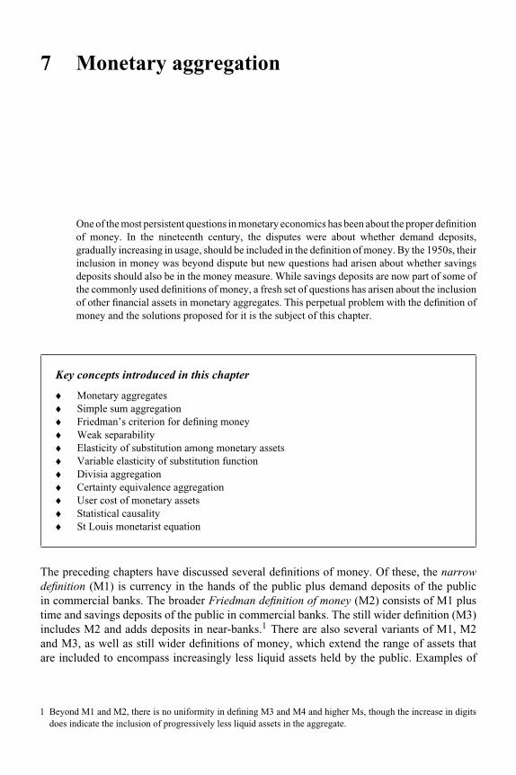
7 Monetary aggregation
One of the most persistent questions in monetary economics has been about the proper definitionof money. In the nineteenth century, the disputes were about whether demand deposits,gradually increasing in usage, should be included in the definition of money. By the 1950s, theirinclusion in money was beyond dispute but new questions had arisen about whether savingsdeposits should also be in the money measure. While savings deposits are now part of some ofthe commonly used definitions of money, a fresh set of questions has arisen about the inclusionof other financial assets in monetary aggregates. This perpetual problem with the definition ofmoney and the solutions proposed for it is the subject of this chapter.
Key concepts introduced in this chapter
♦ Monetary aggregates♦ Simple sum aggregation♦ Friedman’s criterion for defining money♦ Weak separability♦ Elasticity of substitution among monetary assets♦ Variable elasticity of substitution function♦ Divisia aggregation♦ Certainty equivalence aggregation♦ User cost of monetary assets♦ Statistical causality♦ St Louis monetarist equation
The preceding chapters have discussed several definitions of money. Of these, the narrowdefinition (M1) is currency in the hands of the public plus demand deposits of the publicin commercial banks. The broader Friedman definition of money (M2) consists of M1 plustime and savings deposits of the public in commercial banks. The still wider definition (M3)includes M2 and adds deposits in near-banks.1 There are also several variants of M1, M2and M3, as well as still wider definitions of money, which extend the range of assets thatare included to encompass increasingly less liquid assets held by the public. Examples of
1 Beyond M1 and M2, there is no uniformity in defining M3 and M4 and higher Ms, though the increase in digitsdoes indicate the inclusion of progressively less liquid assets in the aggregate.

206 The demand for money
such assets are Treasury bills and money market mutual funds. The very broad monetaryaggregates merge the concept of money in the diffuse concept of “liquidity.”
Given the possibility of many definitions of money, the basis on which the definitionsare arrived at and their relative validity and performance become essential to any empiricalstudy on money. This basis can be purely theoretical, using the functions of money andconcentrating on its role as a medium of exchange and payments. However, as discussedin earlier chapters, this procedure does not normally provide a unique definition of money.Financial assets are created and numerous close substitutes to currency and demand depositscan be easily created in an unregulated, free-enterprise financial system. A plethora of suchassets usually exists in developed economies with unregulated financial markets, so that anempirical basis for including some of these in the definition of money and excluding others isneeded. One of these procedures is provided by the theory of aggregation or composite goods,since any measure of money is an aggregate or composite of its component assets. Aggregationtheory requires weak separability among the assets to be included in the monetary aggregate,so that a test for weak separability provides a mechanism for judging the validity of the assetsto be included in the monetary aggregate.
Once the assets to be included in the definition of money have been selected, the form ofthe aggregator function over the component assets has to be determined. This function canbe specified on an a priori basis or determined by the data. Its common forms in the monetaryliterature are the simple sum aggregates, the variable or constant elasticity of substitutionfunction and the Divisia aggregator function. The various aggregates in turn have to be testedfor their empirical usefulness. The above forms of aggregation and commonly used tests forchoosing among them are presented in this chapter.
Section 7.1 points out the failure of monetary theory to provide a unique definition of moneywhen there are several close but not perfect substitutes for currency and demand deposits,and therefore the rest of this chapter examines the empirical considerations that have beenproposed for selecting among various empirical measures of money. Section 7.2 discussesMilton Friedman’s criterion for empirically defining money. A more rigorous criterion fordefining a composite variable such as money is provided by aggregation theory, whoseweak separability criterion of aggregation is specified in Section 7.3. The four competingmodes of aggregation – simple sum aggregation, variable elasticity of substitution function,Divisia aggregates and certainty equivalence aggregates – are discussed in Sections 7.4, 7.5and 7.8. A moot question arises about the appropriate cost of holding and using money. Ifmoney is used for its liquidity services in financing transactions, the appropriate measureis the user cost of money. This is defined in Section 7.6. Section 7.9 discusses the variouscriteria for judging among monetary aggregates. Since the Divisia aggregates are among thenewer measures and have many appealing features, the appendix to this chapter presents theirderivation.
7.1 The appropriate definition of money: theoretical considerations
There are several possible ways of selecting a preferred version among the possible variantsof money. One of these ways is the intuitive one of focusing on the functions of money andasserting that the medium-of-payments function is its pre-eminent characteristic, so that onlyassets that perform this function are entitled to be in the definition of money.2 In the United
2 The other functions of money are: store of value, standard of deferred payments and unit of account.
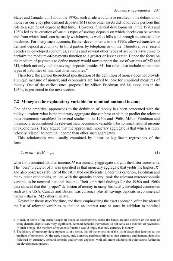
Monetary aggregation 207
States and Canada, until about the 1970s, such a rule would have resulted in the definition ofmoney as currency plus demand deposits (M1) since other assets did not directly perform thisrole to a significant degree at that time.3 However, financial developments in the 1970s and1980s led to the creation of various types of savings deposits on which checks can be writtenand from which funds can be easily withdrawn, as well as bills paid through automatic tellermachines. For many such accounts, further developments in the 1990s allowed transfers todemand deposit accounts or to third parties by telephone or online. Therefore, over recentdecades in developed economies, savings and several other types of accounts have come toperform the medium-of-payments function to a greater or lesser extent. Hence the focus onthe medium of payments to define money would now support the use of variants of M2 andM3, which not only include savings deposits besides M1 but often also include some othertypes of liabilities of financial intermediaries.4
Therefore, the a priori theoretical specification of the definition of money does not providea unique measure of money, and economists are forced to look for empirical measures ofmoney. One of the earliest ones, proposed by Milton Friedman and his associates in the1950s, is presented in the next section.
7.2 Money as the explanatory variable for nominal national income
One of the empirical approaches to the definition of money has been concerned with thepolicy question: what is the monetary aggregate that can best explain or predict the relevantmacroeconomic variables? In several studies in the 1950s and 1960s, Milton Friedman andhis associates considered the relevant macroeconomic variable to be nominal national incomeor expenditures. They argued that the appropriate monetary aggregate is that which is more“closely related” to nominal income than other such aggregates.
This relationship was usually examined by linear or log-linear regressions of theform:
Yt = α0 +α1Mt +μt (1)
where Y is nominal national income, M is a monetary aggregate and μ is the disturbance term.The “best” predictor of Y was specified as that monetary aggregate that yields the highest R2
and also possesses stability of the estimated coefficients. Under this criterion, Friedman andmany other economists, in line with the quantity theory, took the relevant macroeconomicvariable to be nominal national income. Their empirical findings for the 1950s and 1960sdata showed that the “proper” definition of money in many financially developed economiessuch as the USA, Canada and Britain was currency plus all savings deposits in commercialbanks – that is, M2 rather than M1.
Keynesian theorists of the time, and those emphasizing the asset approach, often broadenedthe list of relevant variables to include an interest rate or rates in addition to nominal
3 In fact, at some of the earlier stages in financial development, while the banks are non-existent or the costs ofusing demand deposits are very significant, demand deposits themselves do not serve as a medium of payments.In such a stage, the medium of payments function would imply that only currency is money.
4 The history of monetary development is, in a sense, that of the extension of the list of assets that function as themedium of payments. At the early stages, only currency performs this role; then currency and demand deposits;followed by currency, demand deposits and savings deposits; with still more additions of other assets further inthe development process.

208 The demand for money
national income. One application of this was to estimate a linear or log-linear equation ofthe form:
Mt/Yt = a0 + a1Rt +μt (2)
where R is the nominal interest rate. The definition of money arrived at through estimationsof (2) usually differed from the Friedman criterion specified by (1), since the two criteria aredifferent.
Further, even if nominal income is the only relevant variable to be explained, financialderegulation and technological innovations since the 1960s have led to shifts in the monetaryaggregate that “best” explains nominal national income, with the results depending upon thecountry as well as the time period of the study. Consequently, there is no clear-cut uniquemeasure of money that has consistently proved to be the “best” one over time for any countryor across countries. For instance, during the 1950s and 1960s, as Friedman showed, moststudies indicated that, for the USA and Canada, M2 was “more closely” related to nationalincome than M1 in terms of R2 and the stability of the estimated relationships. But for the1980s and later decades, M1 appeared to perform better than M2 under this criterion.
7.3 Weak separability
From a rigorous theoretical standpoint, a monetary aggregate is a composite good that mustsatisfy the following weak separability condition required for aggregation.
Assume that there are n goods, X1, . . .,Xm, Xm+1, . . .,Xn, whose quantities are related bythe function F(.) to X , as in:
x = F(x1, . . .,xm,xm+1, . . .,xn) (3)
where:x = utility (or output)xi = quantity or real value of the ith goodF(.) = utility (or production) function.
Equation (3) can be written as:
x = F( f (x1, . . .,xm),xm+1, . . .,xn) (4)
if and only if Fi/Fj , i, j = 1, . . .,m, is independent of xm+1, . . .,xn. Fi = ∂F /∂xi and Fi/Fj isthe marginal rate of substitution (MRS) between Xi and Xj . This independence of the MRSbetween each pair of goods in a group from all other goods not in the group is known as theweak separability of the group from other goods in the overall function. If a collection ofgoods, X1, . . .,Xm, satisfies this condition, we can create a composite good M such that itsquantity index m can be constructed from the quantities of the goods only in the group, so thatwe would have m = f (x1, . . .,xm). Further, changes in the quantities or prices of the goodsnot in the group will not change the relative composition of the composite good. However,they can change the total expenditure on the group and hence the budget constraint for thegroup.5
5 Hence, changes in the price of goods not in the group can cause income effects but not substitution effects in thedemand for goods in the group.

Monetary aggregation 209
Hence, if weak separability holds for X1, . . .,Xm from other goods, (4) can berewritten as:
x = F(m,xm+1, . . .,xn) (5)
where:
m = f (x1, . . .,xm) (6)
f (.) in (6) specifies a sub-utility function, whose form must be used to construct the quantity(real value) of the aggregate m. To derive the optimal values for x1, . . .,xm, the sub-utilityfunction f (.) can be maximized subject to the total expenditures allocated for m, but withoutreference to the prices or quantities bought of xm+1, . . .,xn.
Weak separability and monetary aggregation
If the monetary assets X1, . . .,Xm are currency, demand deposits and near-money assets,and weak separability from other goods holds for them, they can be grouped into a validcomposite monetary aggregate whose quantity depends only on the quantities of its owncomponent assets. The relative demand for the component assets in m would depend onlyon the quantity index m and the prices of X1, . . .,Xm, but not directly upon the quantitiesor prices of the other goods Xm+1, . . .,Xn. If F(.) is the individual’s utility function over allgoods, the remaining goods Xm+1, . . .,Xn could include among them other financial assets,consumption goods, leisure, and any other goods in the individual’s utility function. In thecase where F(.) is the firm’s production function and x is the firm’s output, Xm+1, . . .,Xn
could include among them the firm’s other inputs such as labor, capital, other financial assetsand so on.
The condition of weak separability may be satisfied by different groupings of goods, withsome of these encompassing others. In such a case, the former would be a wider aggregateand would include the latter – narrower aggregates – as subcategories of composite goods,just as M2 includes M1 as a component.
Note that if the monetary aggregate M , including the assets X1, . . .,Xm, satisfies theweak separability condition, its functional form will be specified by the particular formof f (x1, . . .,xm) that satisfies the weak separability condition. A misspecification in the formof the f (.) function would mean that the weak separability condition is violated in the contextof the misspecified function. However, the form of f (.) is normally not known a priori,so empirical work has used a variety of arbitrarily specified forms such as the simple sumaggregate, the variable elasticity of substitution function, the Cobb–Douglas function andmore flexible functional forms.6 Ideally, the functional form applied to the data should be asflexible as possible, so that the data could determine the specific functional form.7
6 Among these are the translog form, the Gorman polar flexible functional form and the Fourier flexible functionalform.
7 Weak separability is determined directly from the data on quantities (Varian, 1983). Another form of groupingcan be based on the quasi-separability of prices. A set of variables is said to be quasi-separable if the expenditureon it is a function only of total utility and the prices of goods in the group, but not of the prices of other goods.

210 The demand for money
Empirical evidence on weak separability of monetary variables
Varian (1983) contributed a pioneering study on judging weak separability among goods,using non-parametric econometric methods. Swofford and Whitney (1987) used Varian’stechnique for US data (from 1970 to 1985) on consumption goods, leisure and variousmonetary aggregates. Several definitions of money were found to be weakly separable fromconsumption goods and leisure, with the broadest measure to do so including currency,demand deposits, checkable deposits and small savings deposits. However, measuresbroad enough to include money market mutual funds were not weakly separable fromconsumption and leisure. Conversely, consumption goods and leisure together were weaklyseparable from monetary assets, but consumption goods alone were not. Our concernis only with the former result. It showed that M1 and M2 were acceptable monetaryaggregates but broader measures than M2 were not. Hence, for the period of their study,the definitions or indices of money that include monetary assets beyond those in M2 – and,therefore, implicitly assume their weak separability from other goods in the economy – aremisspecified.
Note that the assets that meet the weak separability criterion for inclusion in the monetaryaggregate are likely to differ among countries and periods. Further, in view of the considerabledegree of innovation and change in the moneyness of assets in the past several decades, theadmissible assets in the monetary aggregate have been changing and are likely to haveincreased beyond M2 for many countries.
Another study using weak separability is Belongia and Chalfant (1989). These authorsstarted with the assumption that monetary assets were weakly separable from consumptionand only examined weak separability within this category. Using US monthly data overthe brief period from January 1983 to February 1986, they reported that several groups ofassets were weakly separable from others. Among these groups were: (C, DD), (C, DD,NOWs), (C, DD, NOWs, MMMF), where C is currency balances, DD is demand deposits,NOWs are negotiable orders of withdrawal8 and MMMF are money market mutual funds.Hence, Belongia and Chalfant’s results offered a choice among various levels of acceptablemonetary aggregates for further analysis. This multiplicity of weakly separable groups is acommon finding, so that other criteria, such as the Friedman one in Section 7.2 and othersdiscussed later in this chapter, are further needed to select the most useful aggregate fromamong them.
7.4 Simple sum monetary aggregates
We are now going to switch from the theory of aggregation specified in the precedingsection to the practical construction of the usual monetary aggregates, which are aggregationsof the nominal values (Xi)9 rather than the real values (xi) of the assets. However, notethat the assets included in any such aggregates must meet the separability criterion foraggregation.
8 NOWs are essentially a type of checkable savings deposits that can be transferred by negotiable orders ofwithdrawal corresponding to checks, so that NOWs are really a form of checkable deposits.
9 We use here the symbol Xi for the nominal value of the asset i even though it was used as the name of the assetin the preceding section.

Monetary aggregation 211
In defining money, the most common functional form for the monetary aggregate is thesimple-sum aggregate given by:
M = X1 +�iaiXi i = 2,3, . . .m,ai = (1,0) (7)
where:M = nominal value of the monetary aggregateX1 = M1 (currency in the hands of the public plus demand deposits in commercial
banks)Xi = nominal value of the ith liquid asset
In Friedman’s analysis (Friedman and Schwartz, 1963 a,b), the term ai took the value 1 ifinclusion of the ith asset gave a better result in explaining the level of national income thanif it were excluded. However, the general functional form (7) was not exclusive to Friedmanbut was the most common form used in the 1950s and 1960s, and is still the most commonmonetary aggregation function in monetary economics.
A monetary aggregate given by (7) a priori assumes that:
(i) The coefficients ai can take only the value zero or one so that all other values are excluded.Further, there is one-to-one substitution between the included assets.
(ii) An infinite elasticity of substitution exists among the assets with a non-zero coefficient,so that the included assets are perfect substitutes.
A generalization of (7) is a weighted sum aggregate that allows the coefficients ai to take onany positive weights between zero and one. In this case, the monetary aggregate, designatedas M ′, is given by:
M ′ = X1 +�i bi Xi i = 2,3, . . .,m (8)
where, now, 0 ≤ bi ≤ 1. The weight ai is sometimes called the degree of moneyness of asseti and can be specified a priori or on the basis of a statistical procedure. To illustrate the latterin line with Friedman’s procedure for defining money, the values of the coefficients can bedetermined empirically by estimating the equation:
Yt = a0 +�i bi Xit +μt i = 1,2, . . .,m (9)
where Y is nominal national expenditure, μ is a stochastic term and 0 ≤ bi ≤ 1. (9) stilldefines money as that variable that “best” explains national expenditures, and the weightsai of the assets are derived by multiple regression. The coefficient of each additional assetshould decrease as the definition of money is broadened to include assets in a decreasingorder of degree of moneyness. However, there are other criteria besides Friedman’sfor selecting among monetary aggregates, and extension of the definition to (9) is notcommon.
While (7) and (8) both specify simple sum aggregates, this term is usually associatedwith (7). It will henceforth be used in this sense. Many economists object to its underlyingassumption that the elasticity of substitution must be either 0 (between an includedand an excluded asset) or infinity (between any pair of the included assets). Twospecifications of the monetary aggregate that use other elasticities are the variable elasticityof substitution function and the Divisia aggregates. These are presented in the next twosections.
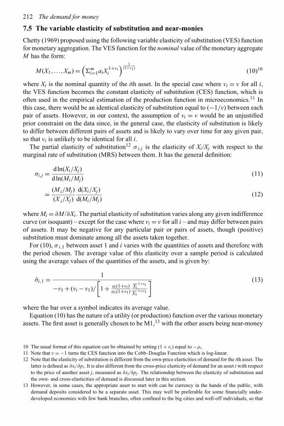
212 The demand for money
7.5 The variable elasticity of substitution and near-monies
Chetty (1969) proposed using the following variable elasticity of substitution (VES) functionfor monetary aggregation. The VES function for the nominal value of the monetary aggregateM has the form:
M (X1, . . .,Xm) =(�m
i=1aiX1+vii
) 1(1+v1)
(10)10
where Xi is the nominal quantity of the ith asset. In the special case where vi = v for all i,the VES function becomes the constant elasticity of substitution (CES) function, which isoften used in the empirical estimation of the production function in microeconomics.11 Inthis case, there would be an identical elasticity of substitution equal to (−1/v) between eachpair of assets. However, in our context, the assumption of vi = v would be an unjustifiedprior constraint on the data since, in the general case, the elasticity of substitution is likelyto differ between different pairs of assets and is likely to vary over time for any given pair,so that vi is unlikely to be identical for all i.
The partial elasticity of substitution12 σ i,j is the elasticity of Xi/Xj with respect to themarginal rate of substitution (MRS) between them. It has the general definition:
σi,j = dln(Xi/Xj)
d ln(Mi/Mj)(11)
= (Mi/Mj)
(X i/Xj)
d(Xi/Xj)
d(Mi/Mj)(12)
where Mi = ∂M /∂Xi. The partial elasticity of substitution varies along any given indifferencecurve (or isoquant) – except for the case where vi = v for all i – and may differ between pairsof assets. It may be negative for any particular pair or pairs of assets, though (positive)substitution must dominate among all the assets taken together.
For (10), σ i,1 between asset 1 and i varies with the quantities of assets and therefore withthe period chosen. The average value of this elasticity over a sample period is calculatedusing the average values of the quantities of the assets, and is given by:
σi,1 = 1
−v1 + (vi − v1)/
[1 + ai(1+vi)
a1(1+v1)Xi
1+vi
X11+v1
] (13)
where the bar over a symbol indicates its average value.Equation (10) has the nature of a utility (or production) function over the various monetary
assets. The first asset is generally chosen to be M1,13 with the other assets being near-money
10 The usual format of this equation can be obtained by setting (1 + vi) equal to −ρi .11 Note that v = −1 turns the CES function into the Cobb–Douglas Function which is log-linear.12 Note that the elasticity of substitution is different from the own-price elasticities of demand for the ith asset. The
latter is defined as ∂xi/∂pi . It is also different from the cross-price elasticity of demand for an asset i with respectto the price of another asset j, measured as ∂xi/∂pj . The relationship between the elasticity of substitution andthe own- and cross-elasticities of demand is discussed later in this section.
13 However, in some cases, the appropriate asset to start with can be currency in the hands of the public, withdemand deposits considered to be a separate asset. This may well be preferable for some financially under-developed economies with few bank branches, often confined to the big cities and well-off individuals, so that

Monetary aggregation 213
or other liquid assets. The monetary aggregate defined by (10) is sometimes referred toas moneyness or liquidity. To derive its estimating equations, assume that the individualmaximizes (10) subject to the budget constraint:
�ipiXi = A (14)
where:pi = price of the ith assetA = expenditures to be allocated over M1 and the other monetary assets.
Maximizing (10) subject to (14) gives the following first-order conditions, with λ as theLagrangian multiplier:
Mi −λpi = 0 where Mi = ∂M/∂Xi, i = 1,2, . . .,m (15)
�ipiXi = A
which yield, for i = 2,3, . . .,
ai(1 + vi)Xvii
a1(1 + v1)X v11
= pi
p1(16)
lnXi = αi + 1
viln
pi
p1+ v1
vilnX1 (17)
where αi = 1
viln
a1(1 + v1)
ai(1 + vi)
Hence, for i = 1,2, . . .,m, the (m − 1) estimating equations for the i assets are of theform:
lnXi = αi + 1
viln
pi
p1+ v1
vilnX1 +μi (16′)
For i > 2, these equations need to be estimated by simultaneous regression techniques soas to meet the cross-equation restrictions on v1. However, it is common to estimate (16′)by single equation regression techniques, as is done by Chetty. Such estimation providesthe estimated values of vi from the coefficient on ln (pi/p1). This value and the estimatedvalue of (v1/vi) from the coefficient on ln X1 yield the estimate for v1. From these values, theestimated values of the average partial elasticities of substitution can be calculated, as givenby (13).14
An important theoretical and empirical issue in the above estimation is that of themeasurement of the prices of financial assets. Viewed from the perspective of mon-etary assets as durable goods (which last beyond the current period), there are two
demand deposits do not constitute a medium of payments for much of the economy. Gebregiorgis and Handa(2005) report that for Nigeria, over the sample period 1970 to 2000, currency did better than other monetaryaggregates such as M1 and M2.
14 One problem that often occurs in VES estimation is that the estimated coefficients (v1/vi) and (1/vi) respectivelyof ln Xi and ln (pi/p1) tend to be quite small, so that the calculation of vi is very sensitive, as is that of theelasticity of substitution, to small differences in the estimated coefficients.

214 The demand for money
alternative ways of defining their prices. One of these is the purchase price, while itsalternative is the user cost of the services rendered by the durable good during theperiod. Chetty (1969) used the former.15 Defining a unit of the ith asset as havinga value of unity at the end of the period, he specified its purchase price (i.e. itspresent discounted value) at the beginning of the period as 1/(1+Ri), where Ri is thenominal rate of return on the asset over the period. Hence, Chetty’s study specifiedpi as:
pi = 1/(1 + Ri) (18)
Designating the non-interest-paying asset 1 as M1 with R1 = 0 implies that p1 = 1, sothat:
pi/p1 = 1/(1 + Ri) i = 2,3, . . . (19)
Empirical findings
We use Chetty’s study for the United States for the period 1945–66 to provide one set offindings based on (17) and (19). This study considered four assets, with i = 1, . . .,4, and usedtheir nominal values to estimate the nominal value M ′ of the monetary aggregate. The fourassets in this study were:
X1 = currency plus demand deposits (M1) in commercial banks (M1)X2 = savings/time deposits in commercial banks (TD)X3 = savings/time deposits in mutual savings banks (TDM)X4 = savings and loan associations shares (SLS).
Chetty’s estimates of their elasticities of substitution, designated as σ 1,i, between moneyand the ith assets, were:
σ1,2 = σM1,TD = 30.864
σ1,3 = σM1,TDM = 35.461
σ1,4 = σM1,SLS = 23.310
Chetty interpreted these magnitudes as indicating that all three near-money assets weregood substitutes for money. The estimated form of the monetary aggregate M was:
M =[X 0.954
1 + 1.020X 0.9752 + 0.880X 0.959
3 + 0.615X 0.9814
]1.026(20)
Since the exponents of the variables on the right-hand side of (20) were close to one, as isthe coefficient of X2, M was approximated by Chetty as:
M = X1 + X2 + 0.880X3 + 0.615X4 (21)
15 This definition of the price of an asset is not based on its user or rental cost, discussed in Section 7.6 below.More recent contributions in the literature have not used Chetty’s specification of prices but have substituted auser cost definition in its place.

Monetary aggregation 215
The yield RM on this monetary aggregate can be calculated as a correspondingly weightedindex of interest rates on the near-money assets, so that it was specified as:
RM = (R2 + 0.880R3 + 0.615R4)/(1 + 0.88 + 0.615) (22)
Chetty’s estimation of the elasticities of substitution, by his single equation estimationand by his use of the cost rather than the user cost of assets, though limited in its usefulnessby the form of the aggregation function specified a priori as (10), is valuable for providingan empirical procedure for estimating the degree of substitution between money and near-money assets. His results basically confirmed the general perception by economists inthe 1960s of the close substitution between money and several other financial assets, andsupported the evidence derived from estimates of the money demand function. Note thatthe financial deregulation and the considerable technological innovation in the financialsector in the USA since the 1960s have changed the elasticities of substitution fromthose reported by Chetty and have also created many new near-money assets, so that themonetary aggregate implied by estimating (17) would now be different from that derived byChetty.
The VES (or CES) function estimates the elasticities of substitution which directly reflectthe degree of substitution between money and near-money assets and are directly related tothe debate on the appropriate definition of money, while the empirical studies of the demandfor money function estimate the own- and cross-interest elasticities of the demand for money.The estimated values of the own- and cross-price elasticities are usually less than one, whichare of a different order of magnitude from the elasticities of substitution reported by Chetty,so that we need a procedure for comparing the two concepts.
Comparison of elasticities of substitution with price elasticities
The elasticities of substitution are not directly comparable with price elasticities but are acomponent of the latter, and the two are difficult to compare for the general case. However,Feige and Pearce (1977, p. 461) reported the following relationship for the two-asset case,of which the first one is M1 with R1 = 0.
σ1,2 =(
1 + R2
R2
)[E1,2 − E2,2
](23)
where:σ 1,2 = elasticity of substitution between asset 1 and asset 2E2,2 = own-price elasticity of asset 2 (with respect to its own price)E1,2 = cross-price elasticity of asset 1 with respect to the return on asset 2R2 = return on asset 2.
To illustrate the reconciliation between the estimated large elasticities of substitution andthe less-than-one price elasticities, let i = 1 for M1 and j = 2 for a near-money asset.Then, if E1,2 = −0.4, E2,2 = 1.0 and R2 = 0.04, (23) implies that σ 1,2 = 36.4, whichis close to the elasticities of substitution reported by Chetty (Feige and Pearce, 1977,p. 460). Hence, small values of own- and cross-price elasticities can be consistent with verylarge elasticities of substitution, so that Chetty’s estimates of the latter are not necessarilyinconsistent with the own- and cross-elasticities usually occurring in the estimated demandfunctions.
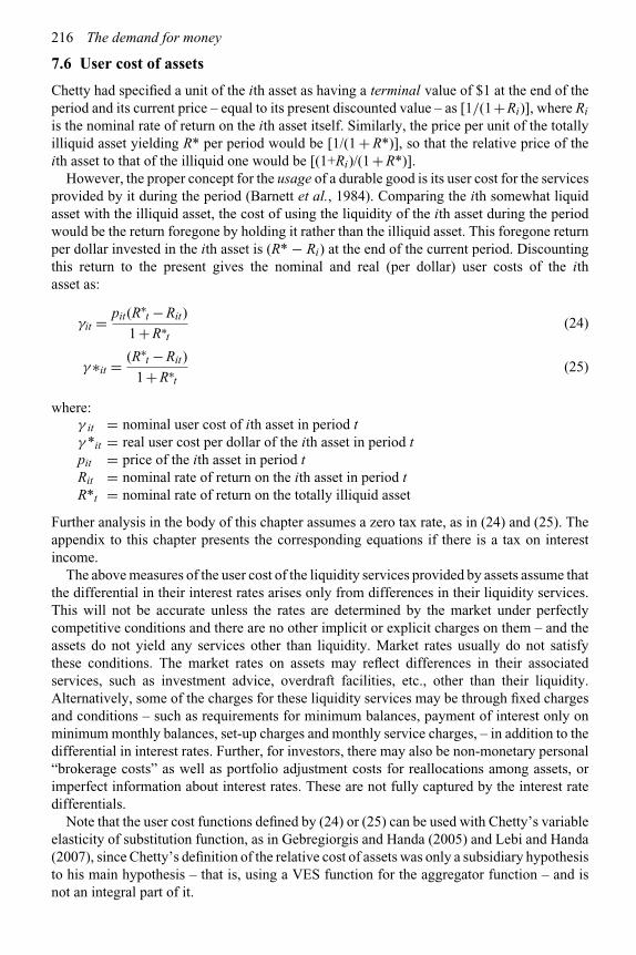
216 The demand for money
7.6 User cost of assets
Chetty had specified a unit of the ith asset as having a terminal value of $1 at the end of theperiod and its current price – equal to its present discounted value – as [1/(1+Ri)], where Ri
is the nominal rate of return on the ith asset itself. Similarly, the price per unit of the totallyilliquid asset yielding R* per period would be [1/(1 + R*)], so that the relative price of theith asset to that of the illiquid one would be [(1+Ri)/(1 + R*)].
However, the proper concept for the usage of a durable good is its user cost for the servicesprovided by it during the period (Barnett et al., 1984). Comparing the ith somewhat liquidasset with the illiquid asset, the cost of using the liquidity of the ith asset during the periodwould be the return foregone by holding it rather than the illiquid asset. This foregone returnper dollar invested in the ith asset is (R* − Ri) at the end of the current period. Discountingthis return to the present gives the nominal and real (per dollar) user costs of the ithasset as:
γit = pit(R∗t − Rit)
1 + R∗t
(24)
γ ∗it = (R∗t − Rit)
1 + R∗t
(25)
where:γ it = nominal user cost of ith asset in period tγ *it = real user cost per dollar of the ith asset in period tpit = price of the ith asset in period tRit = nominal rate of return on the ith asset in period tR*t = nominal rate of return on the totally illiquid asset
Further analysis in the body of this chapter assumes a zero tax rate, as in (24) and (25). Theappendix to this chapter presents the corresponding equations if there is a tax on interestincome.
The above measures of the user cost of the liquidity services provided by assets assume thatthe differential in their interest rates arises only from differences in their liquidity services.This will not be accurate unless the rates are determined by the market under perfectlycompetitive conditions and there are no other implicit or explicit charges on them – and theassets do not yield any services other than liquidity. Market rates usually do not satisfythese conditions. The market rates on assets may reflect differences in their associatedservices, such as investment advice, overdraft facilities, etc., other than their liquidity.Alternatively, some of the charges for these liquidity services may be through fixed chargesand conditions – such as requirements for minimum balances, payment of interest only onminimum monthly balances, set-up charges and monthly service charges, – in addition to thedifferential in interest rates. Further, for investors, there may also be non-monetary personal“brokerage costs” as well as portfolio adjustment costs for reallocations among assets, orimperfect information about interest rates. These are not fully captured by the interest ratedifferentials.
Note that the user cost functions defined by (24) or (25) can be used with Chetty’s variableelasticity of substitution function, as in Gebregiorgis and Handa (2005) and Lebi and Handa(2007), since Chetty’s definition of the relative cost of assets was only a subsidiary hypothesisto his main hypothesis – that is, using a VES function for the aggregator function – and isnot an integral part of it.

Monetary aggregation 217
7.7 Index number theory and Divisia aggregates
Another approach to monetary aggregation is based on statistical index number theoryand focuses on quantity and price data, rather than on utility or production functions,emphasizing the desirable properties of indices.16 Among the statistically desired propertiesof an index number are that any changes in the prices of the components of theindex change only the price index and any changes in the quantities of the compo-nents change only the quantity index, while the multiple of the price and the quantityindices thus computed equals the index of the expenditures on the services of theassets. The simple-sum aggregates do not meet several of these properties. One aggregatethat does meet more of these properties is the Divisia aggregate, first proposed byFrançois Divisia in 1925. The Divisia quantity and price indices possess the desiredproperties and make it tempting to select the Divisia quantity aggregate as the appro-priate aggregator function for monetary assets.17 The development and popularizationof the (Törnqvist–Theil) Divisia monetary aggregate was initiated by Barnett (1980),who proposed the chain-weighted functional form, discussed later in this section, of thisaggregate.
The Divisia quantity aggregate xt(x1t, . . .,xmt) for the m monetary assets for the period tis given by:
xt(x1t, . . .,xmt) =m∏
i=1
xsitit (26)
where:xt = Divisia aggregate for period tsit = share of the ith asset in the expenditure on liquidity services in period tm∏
i=1= product, from 1 to m.
On the general nature of the Divisia index, (26) specifies the Divisia quantity aggregate asa CES (constant elasticity of substitution) function in which the elasticity of substitution isconstant and identical at unity within each period.18 Therefore, the functional form of theDivisia quantity aggregate xt , as specified by (26), is the Cobb–Douglas one, so that it isessentially a weighted log-linear sum of the component assets, as in:
ln xt = �isit ln xit i = 1, . . .,m (27)
Further, (26) implies the computationally appealing growth equation:
xt =m∑
i=1
sit xit (28)
16 Irving Fisher presented in the 1920s a detailed analysis of index numbers and their properties. Among theindex numbers specified by him were the Laspeyres, the Paasche and Fisher’s Ideal index, the last one being ageometric average of the former two.
17 Divisia aggregates are part of a class of statistical index numbers which are sometimes designated as“superlative.”
18 Note in this connection that, for vi = v = −1 for all i, the VES function in (10) becomes the Cobb–Douglas one.
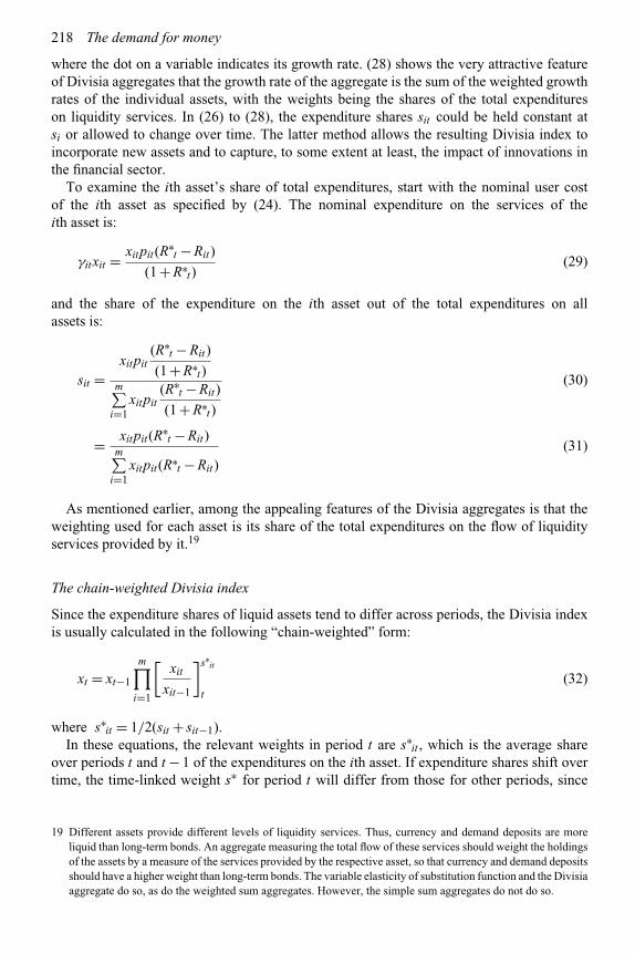
218 The demand for money
where the dot on a variable indicates its growth rate. (28) shows the very attractive featureof Divisia aggregates that the growth rate of the aggregate is the sum of the weighted growthrates of the individual assets, with the weights being the shares of the total expenditureson liquidity services. In (26) to (28), the expenditure shares sit could be held constant atsi or allowed to change over time. The latter method allows the resulting Divisia index toincorporate new assets and to capture, to some extent at least, the impact of innovations inthe financial sector.
To examine the ith asset’s share of total expenditures, start with the nominal user costof the ith asset as specified by (24). The nominal expenditure on the services of theith asset is:
γitxit = xitpit(R∗t − Rit)
(1 + R∗t)
(29)
and the share of the expenditure on the ith asset out of the total expenditures on allassets is:
sit =xitpit
(R∗t − Rit)
(1 + R∗t)
m∑i=1
xitpit(R∗
t − Rit)
(1 + R∗t)
(30)
= xitpit(R∗t − Rit)
m∑i=1
xitpit(R∗t − Rit)
(31)
As mentioned earlier, among the appealing features of the Divisia aggregates is that theweighting used for each asset is its share of the total expenditures on the flow of liquidityservices provided by it.19
The chain-weighted Divisia index
Since the expenditure shares of liquid assets tend to differ across periods, the Divisia indexis usually calculated in the following “chain-weighted” form:
xt = xt−1
m∏i=1
[xit
xit−1
]s∗it
t(32)
where s∗it = 1/2(sit + sit−1).
In these equations, the relevant weights in period t are s∗it , which is the average share
over periods t and t − 1 of the expenditures on the ith asset. If expenditure shares shift overtime, the time-linked weight s∗ for period t will differ from those for other periods, since
19 Different assets provide different levels of liquidity services. Thus, currency and demand deposits are moreliquid than long-term bonds. An aggregate measuring the total flow of these services should weight the holdingsof the assets by a measure of the services provided by the respective asset, so that currency and demand depositsshould have a higher weight than long-term bonds. The variable elasticity of substitution function and the Divisiaaggregate do so, as do the weighted sum aggregates. However, the simple sum aggregates do not do so.

Monetary aggregation 219
for instance, s∗it will be the average of the expenditure shares sit and sit−1, while s∗
it+1 willbe the average of the expenditure shares sit+1 and sit . The log-linear version of this Divisiaquantity index provides the rate of change between periods t and t−1 as:
ln xt − ln xt−1 = �is∗it(ln xit − ln xit−1) (33)
Since the resulting index takes account of changes in expenditures over time on the liquidassets, it will capture the impact of those innovations that alter the relative liquidity anddemands of the component assets, which makes it preferable to an index that uses constantexpenditure shares.
Economic theory and the appropriate form of aggregation
From an economic theoretic viewpoint, the appropriate form of the aggregation function is thatwhich replicates actual economic behavior, whether or not it suits mathematical convenienceor the desirable statistical properties of indices. Monetary theory does not prescribe thisform, so it has to be determined by the data itself. There is no a priori reason why thedata need necessarily behave according to the Divisia format, which requires a constantunit elasticity of substitution within a given period between each pair of its componentassets. To illustrate this point for a financially developed economy, we expect, on the basisof our a priori knowledge, that the component assets (currency and demand deposits) ofM1 possess high elasticities of substitution between them. This would make the Divisiaaggregate of currency and demand deposits a poor approximation to the actual aggregateunderlying the data. One way around this criticism is to rely on our a priori intuitiveknowledge to combine simple sum aggregation and Divisia aggregation. In line with this,for financially developed economies, the Divisia aggregate is often constructed by using M1as its most liquid asset, where M1 is the simple sum aggregate of currency in the handsof the public plus demand deposits in commercial banks. The unit elasticity assumption isthen imposed between M1 and each of the other distinct assets, such as savings deposits,to construct a Divisia aggregate. But if savings deposits are almost perfect substitutes forM1, then M2 (= M1 + S) will be the primary asset in the construction of the Divisiaindex. This mode of construction is appealing because it uses common sense to blendthe various convenient forms of aggregation. However, we still cannot be sure that thisconstruct rather than another alternative, possibly with a different elasticity of substitutionthan unity, is the most appropriate one between M2 and other monetary assets for a givendata set.20 It is therefore necessary to construct and use appropriate statistical tests tojudge the relative usefulness of the various aggregates. Such tests are presented later inthis chapter.
7.8 The certainty equivalence monetary aggregate
Rotemberg (1991) and Rotemberg et al. (1995) proposed what they called the “currencyequivalence” monetary aggregate (CEM) over the monetary assets. This too is a time-varyingweighted average of the component assets but differs from the Divisia aggregates in that it
20 For instance, if the data is generated by a scenario where the elasticities of substitution are considerably in excessof unity for some pairs of assets and zero among others.

220 The demand for money
uses somewhat different weights from the latter. The functional form of the CEM aggregatefor the weakly separable set of monetary assets is:
ln CEMt =m∑
i=1
θit ln xit θit = (R∗t − Rit)/R∗
t . (34)
where xi is the quantity of the ith asset, R∗ is the nominal yield on a totally illiquidasset and Rit is the yield on asset i. The CEM index is log-linear, as is the Divisia one,so that it incorporates the assumption of identical elasticity of substitution equal to unitybetween each pair of assets. However, the CE index specifies θit as (R∗
t − Rit)/R∗t , while
the Divisia aggregate, quite appropriately, defines user cost by (R∗t – Rit)/(1 + R∗
t). Thelatter is preferable since its denominator is the appropriate mode of discounting fromthe end of the period to its beginning. However, if θit (= (R∗
t – Rit)/R∗t) is viewed
as an approximation of user cost, it becomes similar to the Divisia index, but withthe property that the asset (presumably, currency) with Rit = 0 will have a weight ofunity.21
The Divisia index assigns expenditure shares si (or the time-variant sit), which mustsum to unity, while the CE index assigns weights22 which do not have to sum tounity.23 The CE aggregate has the property that as long as currency (and zero-interestdemand deposits) does not pay interest, its amount has a weight of one. Therefore,by normalizing the liquidity weight of currency (and demand deposits) at unity,24 theinterpretation of the CEM aggregate is that it specifies the amount of currency that wouldyield the same liquidity services as the assets in the monetary aggregate. With time-varying weights, just as for the chain-weighted Divisia aggregates, the CEM aggregatealso adapts easily over time to reflect changes in the payments environment. While theperformance of the CEM aggregate relative to its alternatives remains an open empiricalquestion, the simple-sum and Divisia aggregates remain the more common modes of monetaryaggregation.
7.9 Judging among the monetary aggregates
While the economist can decide on the appropriate level of aggregation on an a prioribasis, this is often not a satisfactory procedure for empirical applications since the empiricalcharacteristics of assets vary over periods and economies. Monetary economics therefore hasa variety of empirical criteria for selecting among various aggregation procedures. One ofthese, the Friedman test, has already been discussed earlier in this chapter. In the following,we assume that weak separability tests were performed to determine the assets that have
21 Serletis and Molik (1999, p. 106) describe Rotemberg’s CE index as a “(logarithmic) simple-sum index with asimple weighting mechanism added.” However, it seems preferable to view the CE index as an approximationto the Divisia one, since, within a period, it shares with the latter the property of unit elasticity of substitutionbetween pairs of assets and allows time-varying weights.
22 At the practical level of computing user costs, Rotemberg recommended using the return on common stocks asthe benchmark rate – as opposed to using a long-term bond, which Barnett does – since all bonds offer somedegree of liquidity services. This may bias the calculations on the user cost and expenditure shares.
23 Given the uncertainty of the yields on assets, both CE and Divisia indices should properly use the expected(rather than actual) returns in deriving user costs and expenditure shares.
24 By comparison, their weights in a Divisia index would be very much smaller than one.

Monetary aggregation 221
been included in the aggregate, and that the choice that has to be exercised is between thefunctional forms of the aggregate.
7.9.1 Stability of the money demand function
If the estimated demand function for a monetary aggregate is to be useful for prediction, itshould have a high R2 and be stable over different sample periods. If the function is not stable,its value for predicting money demand in future periods and for policy purposes is limited.While this requirement may not seem to be very stringent, it is not always satisfied andrejects many of the estimated demand functions. For instance, the money-demand functionsestimated for 1980s and 1990s for most of the commonly used monetary aggregates show ahigh degree of instability for many countries.
7.9.2 Controllability of the monetary aggregate and policy instrumentsand targets
If the central bank is to consider the monetary aggregate useful for policy purposes, thebank must be able to control it through the policy instruments at its disposal. Assuming thatthe central bank uses the nominal monetary base M0 as its control instrument, it will beconcerned with the relationship between M0 and the monetary aggregate M . A simple linearrelationship between M and M0 is given by:
M = a0 + a1M0 (35)
where:M = nominal value of the monetary aggregateM0 = nominal value of the monetary basea1 = monetary base-money multiplier (∂M /∂M0)
The central bank can control M through M0 only if a0 and a1 are stable. Different monetaryaggregates possess different values of these coefficients with different degrees of stability.The preferred aggregate would be one with stable values of the coefficients and a high R2 inestimations.
Note that this criterion becomes irrelevant if the central bank does not believe that itsmanipulation of monetary aggregates confers a predictable benefit in terms of aggregatedemand and its final goal variables, such as output and unemployment. In fact, many centralbanks now hold the view that manipulation of the interest rate provides better control overthese variables, so that there is a general tendency to downplay the relevance of monetaryaggregates (see Chapter 13).
7.9.3 Causality from the monetary aggregate to income
Take a policy instrument X , which could be a monetary aggregate or an interest rate. Tobe useful for controlling nominal national income Y , changes in X should cause changesin Y . The statistical procedure for determining causation between variables is the Granger–Sims test for causality. This procedure is a statistical determination of causality and judges(statistical) causality to go from a variable X to Y – that is, a change in X causes a change inY – if the data on them shows a lag in the impact of X on Y . That is, if the lagged values of Xare significant in a regression of Y on X , X is said to Granger-cause Y . If the expected future

222 The demand for money
values of X are significant, Y is said to Granger-cause X .25 If both the lagged and the futurevalues of X are significant, Granger causality runs two-way between X and Y . Hence, lagsand/or leads are essential for this procedure to give any results on causality; this proceduredoes not detect causality if there are no leads or lags but only a contemporaneous impactfrom X to Y , or from Y to X .
Sims (1972), in an early application of the Granger procedure for statistical causalityto the relationship between money and income, defined one-way statistical causalitythus:
If and only if causality runs one way from current and past values of some listof exogenous variables to a given endogenous variable, then in a regression of theendogenous variable on past, current, and future values of the exogenous variables, thefuture values of the exogenous variables should have zero coefficients.
(Sims, 1972, p. 541).
This test relies on regression analysis to determine the pattern of lags among the variables.If nominal national income Y is the endogenous variable and the exogenous variables arethe policy instrument X and other variables Z , the relevant regression equation is of theform:
Yt = �iaiXt−i +�ibiZt−i +�iγiYt−i +�jcjXt+j +μt (36)
where Z is the vector of variables other than X and Y and μ is the error term. Note that (36)includes not only the current and lagged values of X , Z and Y but also some future valuesof X through the term �j cj Xt+j . If the estimated coefficients of X are statistically differentfrom zero but those of its future terms are zero, then one-way Granger causality is said toexist from X to Y .
Usually a similar regression is also run with X as the dependent variable and Y among theindependent ones. Such a regression would be of the form:
Xt = �iαiYt−i +�iβiZt−i +�iλiXt−i +�jkjYt+j +μt (37)
For this regression, with X on the left side, one-way causality from Y to X requires that thecoefficients of the lagged values of Y be significantly different from zero, while those of itsfuture values be zero.
Two-way causality between X and Y exists in (36) if both the lagged and the future termsin X have non-zero coefficients. This can be verified from (37) if both the lagged and futureterms in Y have non-zero coefficients. We illustrate these remarks and the nature of theGranger causality test by a simple example where:
Yt = a1Xt + a2Xt−1 + a3Xt+1 +μt (38)
25 If economic theory implies such an impact, the following specification of this procedure will lead to erroneousconclusions on the direction of causality.
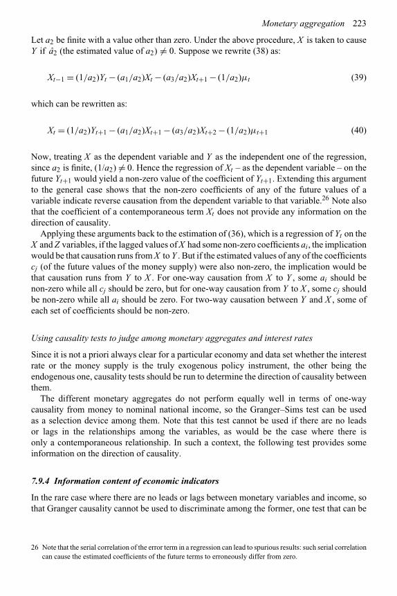
Monetary aggregation 223
Let a2 be finite with a value other than zero. Under the above procedure, X is taken to causeY if â2 (the estimated value of a2) = 0. Suppose we rewrite (38) as:
Xt−1 = (1/a2)Yt − (a1/a2)Xt − (a3/a2)Xt+1 − (1/a2)μt (39)
which can be rewritten as:
Xt = (1/a2)Yt+1 − (a1/a2)Xt+1 − (a3/a2)Xt+2 − (1/a2)μt+1 (40)
Now, treating X as the dependent variable and Y as the independent one of the regression,since a2 is finite, (1/a2) = 0. Hence the regression of Xt – as the dependent variable – on thefuture Yt+1 would yield a non-zero value of the coefficient of Yt+1. Extending this argumentto the general case shows that the non-zero coefficients of any of the future values of avariable indicate reverse causation from the dependent variable to that variable.26 Note alsothat the coefficient of a contemporaneous term Xt does not provide any information on thedirection of causality.
Applying these arguments back to the estimation of (36), which is a regression of Yt on theX and Z variables, if the lagged values of X had some non-zero coefficients ai, the implicationwould be that causation runs from X to Y . But if the estimated values of any of the coefficientscj (of the future values of the money supply) were also non-zero, the implication would bethat causation runs from Y to X . For one-way causation from X to Y , some ai should benon-zero while all cj should be zero, but for one-way causation from Y to X , some cj shouldbe non-zero while all ai should be zero. For two-way causation between Y and X , some ofeach set of coefficients should be non-zero.
Using causality tests to judge among monetary aggregates and interest rates
Since it is not a priori always clear for a particular economy and data set whether the interestrate or the money supply is the truly exogenous policy instrument, the other being theendogenous one, causality tests should be run to determine the direction of causality betweenthem.
The different monetary aggregates do not perform equally well in terms of one-waycausality from money to nominal national income, so the Granger–Sims test can be usedas a selection device among them. Note that this test cannot be used if there are no leadsor lags in the relationships among the variables, as would be the case where there isonly a contemporaneous relationship. In such a context, the following test provides someinformation on the direction of causality.
7.9.4 Information content of economic indicators
In the rare case where there are no leads or lags between monetary variables and income, sothat Granger causality cannot be used to discriminate among the former, one test that can be
26 Note that the serial correlation of the error term in a regression can lead to spurious results: such serial correlationcan cause the estimated coefficients of the future terms to erroneously differ from zero.

224 The demand for money
used is one that calculates the “information content” of the stochastic variable X for Y . Forthis test, the stochastic linear model used between Y and X is assumed to be:
Yt = a0 + a1Xt +μt (41)
where μt is white noise. The expected information content of X with respect to Y ismeasured by:
I (Y |X ) = 1
2ln
[1
(1 − R2)
](42)
where R2 is the coefficient of determination. Note that this test uses only the contemporaneousvalues of the variables. A higher value of I (Y |X ) indicates a higher information content ofX for Y , so that the form of X that has a higher value for this statistic would be preferablefor explaining Y .
7.9.5 The St Louis monetarist equation
The reduced-form equation from the short-run macroeconomic IS–LM models with anexogenous money supply for the relationship between nominal national income Y and themoney stock M is:
Y = f (M ,G,Z) (43)
where:Y = nominal national incomeM = vector of past and present nominal values of the appropriate monetary
aggregateG = vector of past and present values of the appropriate fiscal variablesZ = vector of the other independent variables.
The linear or log-linear stochastic form of the above equation, popularized by the St Louismonetarist school (Anderson and Jordan, 1968), was:
Yt = �iaiMt−i +�jbjGt−j +�iciZt−i +�iγiYt−i +μt (44)
Equation (44) is often called the St Louis equation and represents a popular method fordetermining the impact of monetary and fiscal variables on nominal income. It can beestimated in levels or first differences of the variables. There are many different ways ofspecifying the fiscal variable G. Among these is government expenditures and the fiscaldeficit, or their values at full employment. The set of variables in Z also tends to varybetween studies.
The monetary aggregate in (44) can be represented by one of its different forms. To makethe choice among these forms for given versions of the Y , G and Z variables, (44) is estimatedusing different monetary aggregates. These estimates are examined for the signs, significanceand stability of the coefficients. The monetary aggregate that performs “better” – in terms ofthe coefficient of determination, the plausibility of the estimated values of the coefficientsand their stability – is considered preferable to the other aggregates.

Monetary aggregation 225
Since many central banks now use an interest rate as their main policy instrument, theappropriate form of the St Louis equation in this context becomes:
Yt = �iaiRt−i +�jbjGt−j +�iciZt−i +�iγiYt−i +μt (45)
where R is the relevant nominal interest rate. While this equation can be used to judge theinterest rate most relevant to explaining Y , its estimation will not provide any informationon the appropriate form of the monetary aggregate.
7.9.6 Comparing the evidence on Divisia versus simple-sum aggregation
Theoretical considerations
As explained earlier in this chapter, in a fairly static context, simple-sum aggregation betweentwo monetary variables is relatively more appropriate – and therefore likely to perform“better” empirically – than their Divisia aggregate if the two are close substitutes, so thatthey possess a high elasticity of substitution. But their Divisia aggregate is relatively moreappropriate, and likely to do better empirically, for any two assets that have a relativelylow degree of substitution, especially if their elasticity of substitution is close to unity.The wider the existing degree of aggregation, the more likely is an additional asset tofit into the latter case, so that the broader the definition of the monetary aggregate, themore likely is the Divisia aggregate to perform better than its simple-sum counterpart.27
Since the empirical findings depend upon the actual degree of elasticity of substitutionamong assets, a financial innovation that changes this elasticity could alter the results on theappropriate monetary aggregate. In fact, the past several decades have seen a considerableamount of innovation in financial intermediation and in payments technology, causing shiftsin the estimated demand functions for the monetary aggregates and therefore also in therelationships between money and national income. This process has been accompanied byincreases in the liquidity of many assets that are not in M1 and even those not in M2.Divisia aggregates with time-varying weights can capture such shifts through changesin these weights over time. Simple-sum aggregates in their standard form have a fixedweight of unity for each asset in the aggregate and zero for excluded assets, so thattheir rigidity in weights makes them inappropriate for a period of changing liquiditypatterns. Therefore, for broad aggregates and for recent periods, the expectation is thatsimple-sum aggregation is likely to do worse than Divisia aggregation with time-variantweights.
However, while Divisia aggregates are expected to perform better – especially forvery broad aggregates – from a theoretical and statistical perspective under a changingpayments technology, the simple-sum aggregates retain their popularity for the public andthe policy makers. The latter are easier to grasp and compute, whereas the former requireintricate calculations. Further, if the Divisia aggregates are to be responsive to the changing
27 Note that if the rates of return on both currency and demand deposits are zero and their non-monetary costs areignored, the user cost of the two would be identical. This would impart a degree of similarity in their weightingin Divisia aggregation. Barnett et al. (1984) argue that since the return on currency and demand deposits movesimilarly, their simple-sum aggregate M1 and its Divisia aggregate DM1 tend to perform similarly under thevarious criteria.
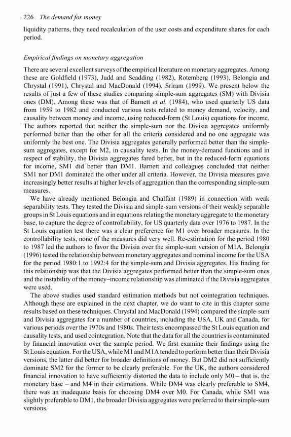
226 The demand for money
liquidity patterns, they need recalculation of the user costs and expenditure shares for eachperiod.
Empirical findings on monetary aggregation
There are several excellent surveys of the empirical literature on monetary aggregates. Amongthese are Goldfield (1973), Judd and Scadding (1982), Rotemberg (1993), Belongia andChrystal (1991), Chrystal and MacDonald (1994), Sriram (1999). We present below theresults of just a few of these studies comparing simple-sum aggregates (SM) with Divisiaones (DM). Among these was that of Barnett et al. (1984), who used quarterly US datafrom 1959 to 1982 and conducted various tests related to money demand, velocity, andcausality between money and income, using reduced-form (St Louis) equations for income.The authors reported that neither the simple-sum nor the Divisia aggregates uniformlyperformed better than the other for all the criteria considered and no one aggregate wasuniformly the best one. The Divisia aggregates generally performed better than the simple-sum aggregates, except for M2, in causality tests. In the money-demand functions and inrespect of stability, the Divisia aggregates fared better, but in the reduced-form equationsfor income, SM1 did better than DM1. Barnett and colleagues concluded that neitherSM1 nor DM1 dominated the other under all criteria. However, the Divisia measures gaveincreasingly better results at higher levels of aggregation than the corresponding simple-summeasures.
We have already mentioned Belongia and Chalfant (1989) in connection with weakseparability tests. They tested the Divisia and simple-sum versions of their weakly separablegroups in St Louis equations and in equations relating the monetary aggregate to the monetarybase, to capture the degree of controllability, for US quarterly data over 1976 to 1987. In theSt Louis equation test there was a clear preference for M1 over broader measures. In thecontrollability tests, none of the measures did very well. Re-estimation for the period 1980to 1987 led the authors to favor the Divisia over the simple-sum version of M1A. Belongia(1996) tested the relationship between monetary aggregates and nominal income for the USAfor the period 1980:1 to 1992:4 for the simple-sum and Divisia aggregates. His finding forthis relationship was that the Divisia aggregates performed better than the simple-sum onesand the instability of the money–income relationship was eliminated if the Divisia aggregateswere used.
The above studies used standard estimation methods but not cointegration techniques.Although these are explained in the next chapter, we do want to cite in this chapter someresults based on these techniques. Chrystal and MacDonald (1994) compared the simple-sumand Divisia aggregates for a number of countries, including the USA, UK and Canada, forvarious periods over the 1970s and 1980s. Their tests encompassed the St Louis equation andcausality tests, and used cointegration. Note that the data for all the countries is contaminatedby financial innovation over the sample period. We first examine their findings using theSt Louis equation. For the USA, while M1 and M1A tended to perform better than their Divisiaversions, the latter did better for broader definitions of money. But DM2 did not sufficientlydominate SM2 for the former to be clearly preferable. For the UK, the authors consideredfinancial innovation to have sufficiently distorted the data to include only M0 – that is, themonetary base – and M4 in their estimations. While DM4 was clearly preferable to SM4,there was an inadequate basis for choosing DM4 over M0. For Canada, while SM1 wasslightly preferable to DM1, the broader Divisia aggregates were preferred to their simple-sumversions.

Monetary aggregation 227
For the causality tests, Chrystal and MacDonald considered it important to include aninterest rate in their cointegration and error correction models. For the UK and Canada,both the Divisia and the simple-sum aggregates showed little causal impact on real output.For the USA, the Divisia measures were significant but not the simple-sum measures. Theoverall comparison, based on both the St Louis equation and the causality tests, did not,therefore, strongly favor one of the aggregates, though there was somewhat stronger supportfor the broad Divisia aggregates over the corresponding broad simple-sum aggregates. For theUSA, Chrystal and MacDonald found that this was especially so after 1980, when financialinnovation occurred at a faster rate. By comparison, pre-1980 US data did not favor theDivisia aggregates.28
Gebregiorgis and Handa (2005) estimate simple-sum, VES and Divisia aggregates,employing the user cost concept, for Nigeria for the period 1970:1 to 2000:4 and examinetheir relative performance, using cointegration analysis, for the determination of industrialproduction. Contrary to the usual findings for developed economies, this study reportsthat for Nigeria currency did as well as or better than any narrow- or broad-moneymeasure. However, this need not be surprising since most of the population of Nigeriadoes not have access to or utilize banking facilities. Further, they report that simple-sumaggregates of M1 and M2 do better than their VES and Divisia counterparts. In fact,Divisia M2 does worse than currency and the simple-sum and VES aggregates for M1and M2.29
Lebi and Handa (2007) study monetary aggregation at the M2 level for Canada, usingthe various tests outlined in this chapter to judge among them. Statistical problems thatarose in its construction made it impossible to construct the VES aggregate for M2. Theirfinding is that the Divisia and currency equivalence M2 indices perform comparably well inmost tests, with CEM2 marginally outperforming DVM2 in the information criterion and theSt Louis equation tests. The simple-sum measure SSM2 dominates in the Granger causalitytests between money and income, and also performs moderately well in the St Louis equationtests.30 In general, the econometric estimates from the cointegration analysis for the money-demand functions do not indicate a clear winner as the monetary aggregate of choice. Theauthors conclude that no one monetary aggregate dominates all others in meeting each of thepossible criteria.
To conclude, neither the simple-sum nor the Divisia aggregates do better than the otherfor all levels of aggregation, all relevant tests and all periods. There is usually no cleardominance of DM1 over SM1, and the two measures have very similar growth rates. But,in general, the broader the aggregate, the more likely is the Divisia measure to performbetter. This is especially so for Divisia aggregates with time-varying weights. However, note
28 Serletis and Robb (1986) found a low degree of substitution among the monetary assets in Canada and littlejustification for M2 and broader aggregates. Their study favored the Divisia aggregates over the simple-sumaggregates.
29 They reasoned that among the segment of Nigeria’s population, mostly in the major urban centers, that useschecking accounts on a regular basis, the elasticity of substitution between currency and checking deposits islikely to be very high, whereas it is likely to be closer to zero in the rural areas with limited banking facilities.While one cannot a priori predict the elasticity of substitution between currency and checking deposits in theaggregate data, a variable elasticity of substitution (VES) function should have a better likelihood of doing aswell as or better than a Divisia one.
30 It should be noted that in cases of divergence between the results from the tests in the levels of the variables andtheir first differences, the latter are preferred.

228 The demand for money
that, as aggregation is broadened to include assets with very low substitution elasticities,further broadening of the Divisia aggregate makes little difference to the performance of theaggregate.
7.10 Current research and policy perspectives onmonetary aggregation
As already mentioned at various points in this chapter, the demand for monetary aggregateshas proved to be unstable in recent periods, largely because of innovations in thevariety of monetary assets and modes of payment. This led a Governor of the Bankof Canada to remark at one point that the Bank did not abandon monetary aggregates,they abandoned central banks as an effective policy instrument. The result has been thatmany central banks in the developed economies have given up control over monetaryaggregates in favor of interest rates as the main policy instrument for controlling aggregatedemand.
In line with this development, monetary economists seem to have lost interest in theestimation of monetary aggregates, so that few significantly new studies have appeared onthis topic since about 1990. Further, whatever limited interest there remains in monetaryaggregates, the focus seems to have shifted from Divisia and other complex forms ofaggregation back to simple forms, which are more readily understood by policy makersand the public.
Conclusions
The starting point for any aggregation is to establish weak separability among the assetswhich are to be included in the aggregate. Once this has been established, the next choiceis to construct a simple-sum aggregate, a variable elasticity of substitution aggregate, and aDivisia or some other aggregate. However, the usual comparison in the literature is betweenthe simple-sum aggregates and the Divisia aggregates, largely because of problems in reliableestimates of the variable elasticity of substitution.
Simple-sum aggregation assumes a priori infinite elasticities of substitution between eachpair of the component assets of the aggregate, and Divisia aggregation assumes a prioriunit elasticity between each pair of the component assets of its aggregate. Intuitively,the former will tend to be the relevant one if the empirical elasticities of substitutionare high, and the latter if they are low. Thus the public’s currency balances and demanddeposits in developed financial sectors tend to be almost perfect substitutes and theirsimple-sum aggregate would be the more appropriate one. In fact, even the commonconstructs of the Divisia aggregates start with the simple-sum aggregate M1 for currencyand demand deposits as the base aggregate. However, in less developed economies withpoor banking facilities in the rural areas and with high brokerage costs of banking, therural public’s currency balances and demand deposits are likely to have limited elasticityof substitution, so that their Divisia aggregation may be more appropriate in such acontext.
For the financially developed economies, the simple-sum M1, composed of currency inthe hands of the public and demand deposits in commercial banks, is usually taken as oneunified asset in constructing the broader Divisia aggregates. Further, since the return onM1 is usually taken to be zero, its rental cost would be higher than of any other asset

Monetary aggregation 229
with a positive rate of return, giving it a correspondingly higher weight in the Divisiaaggregate.
While the Divisia aggregates are superior in terms of desirable index number properties,their a priori assumption of the unit elasticity of substitution limits their usefulness foraggregation over assets that are very close substitutes – and therefore have elasticities ofsubstitution that are substantially higher than unity. Intuitive knowledge of the financialmarkets strongly indicates that there exist several near-monies31 that are close substitutesfor money and would have numerically very high elasticities of substitution. In fact, bothintuition and Chetty’s procedure, though it poses problems in estimation, do indicate thatmany of the financial assets can have very high elasticities of substitution.
As the aggregation is broadened to bring in more and more assets into the aggregate, theadditional assets are likely to have successively lower elasticities of substitution with currencybalances and demand deposits, so that Divisia – as against simple-sum – aggregation becomescorrespondingly more relevant to the further broadening of the aggregate. In general, there isno a priori procedure for deciding which aggregation procedure is better over various groupsof assets.
In a dynamic context with innovation changing the liquidity weights, user costs andexpenditure shares over time, the Divisia aggregates have the advantage that the relativeshares or weights of the assets are allowed to vary over time, so that the computedindex has a flexibility not available to simple-sum aggregates in capturing the impactof innovations. The former are therefore likely to perform better than the latter in adynamic period of financial and technical innovation. However, they have not always donebetter than simple-sum aggregates in different types of empirical tests; so that there is noconvincing evidence that the former unambiguously dominate over the latter. Given thislack of convincing evidence and the familiarity and ease of computation of simple-sumaggregates, these aggregates continue to maintain their popularity for the policy makers,the public and much of the economics profession. Sriram (1999) presents the usage of thethree types of monetary aggregates in 38 studies that had employed cointegration techniques,separating them between those based on developed and on developing economies. Of these38 studies surveyed, only one out of twelve for the developed economies had investigatedDivisia aggregation, and only one out of twenty-four for the developing economies haddone so.
Given that different aggregates tend to perform differently under various tests, we concludethat monetary aggregates need to be tailored to different criteria and purposes, so that thefirst step should be to choose the intended use of the monetary aggregate or, alternatively,to first establish a hierarchy among the criteria on some basis of desirability. Further, theprofession might have to settle for the simultaneous use and acceptance of several differentmonetary aggregates, though for different purposes. This, in turn, suggests that the quest fora single all-purpose monetary aggregate should be abandoned. However, for central bankpolicy purposes and announcements, the most appropriate aggregates remain simple-sumones, though at different levels of aggregation.32
31 For example, checkable savings deposits are now very close substitutes for demand deposits for mostindividuals.
32 Few central banks in the major developed economies now claim to use monetary aggregates as their main, orone of the main, policy instruments. One of the few that does so is the European Central Bank, which uses thesimple-sum M3.

230 The demand for money
Appendix: Divisia aggregation
The symbols in this appendix have the following meanings:x Divisia index for the real value of the composite asset “money”xi real value of asset Xi
p Divisia index of the price level of the composite real asset “money”pi price of asset Xi
si share of the expenditures on Xi
γi nominal user cost of Xi
γ ∗i user cost per dollar of Xi
R∗ maximum available yield – called the “benchmark rate” – over the holding periodRi pre-tax nominal yield on the ith assetτ marginal tax rate� product symbol
For Divisia price and quantity aggregates, we want to construct an index of expenditures,px, where:
px = �ipixi (46)
The rate of change of px is given by:
1
px
d(px)
dt= dx
x+ dp
p=
m∑i=1
(xidpi + pidxi)
m∑i=1
pixi
=m∑
i=1
si
[dpi
pi+ dxi
xi
](47)
where si = pixim∑
i=1pixi
(48)
For the Divisia aggregates, we want to impose the conditions that the quantity index x in theoverall index px changes if and only if the quantities (but not the prices) of the componentassets change, and the price index p in the overall index changes if and only if there isa change in the prices (but not in the quantities) of the component assets. Formally, therequired conditions are that:
dx
x=
m∑i=1
sidxi
xi(49)
dp
p=
m∑i=1
sidpi
pi(50)
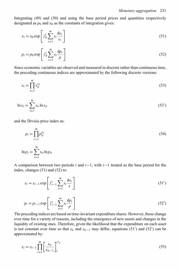
Monetary aggregation 231
Integrating (49) and (50) and using the base period prices and quantities respectivelydesignated as p0 and x0 as the constants of integration gives:
xt = x0 exp
[∫t
0
m∑i=1
sidxi
xi
](51)
pt = p0 exp
[∫t
0
m∑i=1
sidpi
p
](52)
Since economic variables are observed and measured in discrete rather than continuous time,the preceding continuous indices are approximated by the following discrete versions:
xt =m∏
i=1
xsitit (53)
ln xt =m∑
i=1
sit ln xit (53′)
and the Divisia price index as:
pt =m∏
i=1
psitit (54)
lnpt =m∑
i=1
sit lnpit
A comparison between two periods t and t−1, with t−1 treated as the base period for theindex, changes (51) and (52) to:
xt = xt−1 exp
[∫t
t−1
m∑i=1
sidxi
x
](51′)
pt = pt−1 exp
[∫t
t−1
m∑i=1
sidpi
p
](52′)
The preceding indices are based on time-invariant expenditure shares. However, these changeover time for a variety of reasons, including the emergence of new assets and changes in theliquidity of existing ones. Therefore, given the likelihood that the expenditure on each assetis not constant over time so that sit and sit−1 may differ, equations (51′) and (52′) can beapproximated by:
xt = xt−1
m∏i=1
[xit
xit−1
]s∗it
t(55)

232 The demand for money
pt = pt−1
m∏i=1
[pit
pit−1
]s∗it
(56)
s∗it = 1
2(sit + sit−1) (57)
Equations (55) and (56) yield the “chain-weighted” Divisia indices. In these equations,the relevant weights in period t are s∗
it , the average shares over periods t and t−1 of theexpenditures on the ith asset. From (55) and (56), the rates of change in the Divisia quantityand price indices between periods t and t − 1 are given by:
ln xt − ln xt−1 = �is∗it(ln xit − ln xit−1) (58)
lnpt − lnpt−1 = �is∗it(lnpit − lnpit−1) (59)
Measuring prices by the user costs of liquidity services
We now return to the general form of the Divisia index and introduce prices measured byuser costs. The before-tax nominal user cost γit and the real user cost γ ∗
it of the ith asset inperiod t are:
γit = pit(R∗t − Rit)
1 + R∗t
(60)
γ ∗it = (R∗
t − Rit)
1 + R∗t
(61)
Equation (60) specifies the present discounted value of the nominal user cost of holdingthe ith asset. As discussed in the body of the chapter, this user cost is defined for the flow ofliquidity services provided by each asset, with these services assumed to be the only reasonfor the differences in their returns. The numerator (R∗
t −Rit) is the end-of-the-period returnforegone from a dollar of the ith asset for its holding period;33 R∗
t is the interest rate on thetotally illiquid asset.34 Therefore, the denominator (1 + R∗
t) in (60) is the discount factor toconvert the end-of-the-period value to its present (beginning-of-the-period) value using thereturn R∗
t on the most illiquid asset.35 Equation (61) divides the nominal user cost by pt toget the real user cost per dollar invested in the asset.
33 Both interest rates should be over the holding period of the ith asset. However, Ri is usually over a shorterholding period than R∗, which would be the interest rate on a long-term bond. To adjust for the difference inholding period, all rates have to be adjusted to the same maturity.
34 In practice, this asset is taken to be one with the highest interest rate, so that all other assets would have positiveuser costs.
35 Note that this designation (Barnett et al., 1984) of the price or cost of the ith asset differs from that in Chetty(1969). In the present notation and assuming a zero tax rate, Chetty’s measure of the current price of the assetwould have been {1/(1 + Rit )}. It is the present discounted value of $1 obtained at the end of the period fromthe asset i, with the discount factor (1 + Rit ).
As against these two measures, Donovan (1978) defined the price of the ith asset as (1 + Rit )/(1 + R∗t ),
where (1+Rit ) is the amount that one dollar invested in asset Xi in period t would yield at the end of the period,and (1 + Rit )/(1 + R∗
t ) is its present value.

Monetary aggregation 233
The corresponding expenditure share on asset i is specified by:
sit =xitpit
(R∗t − Rit)
(1 + R∗t)
m∑i=1
xitpit(R∗
t − Rit)
(1 + R∗t)
(62)
= xitpit(R∗t − Rit)
m∑i=1
xitpit(R∗t − Rit)
(63)
From (53′) and (63), the Divisia quantity index is given by:
ln xt =m∑
i=1
ln xit
⎡⎢⎢⎣ xitpit(R∗
t − Rit)n∑
i=1xitpit(R∗
t − Rit)
⎤⎥⎥⎦ (64)
Adjustments for taxes on rates of return
If the tax authorities levy a constant tax rate of τ t in period t on interest income but not onliquidity services, the corresponding equations for user cost, shares of expenditures on eachasset and the Divisia quantity index adjusted for this constant tax rate would be as in thefollowing equations:
γit = pit(R∗t − Rit)(1 − τt)
1 + R∗t(1 − τt)
(65)
γ ∗it = (R∗
t − Rit)(1 − τt)
1 + R∗t(1 − τt)
(66)
sit = xitpit(R∗t − Rit)(1 − τ )
m∑i=1
xitpit(R∗t − Rit)(1 − τ )
(67)
ln xt =m∑
i=1
ln xit
⎡⎢⎢⎣ xitpit(R∗
t − Rit)(1 − τt)n∑
i=1xitpit(R∗
t − Rit)(1 − τt)
⎤⎥⎥⎦ (68)
There are thus different ways of defining the price or user cost of an asset. (60) seems preferable to the othermeasures because of its focus in the numerator on the return foregone from holding a liquid asset as against anilliquid one. It also uses the market discount rate on illiquid assets that would be the relevant one for loans tothe individual.

234 The demand for money
Summary of critical conclusions
❖ A simple-sum aggregate assumes perfect substitution – that is, infinite elasticity ofsubstitution – among its components.
❖ The variable elasticity of substitution (VES) monetary aggregate allows the elasticity ofsubstitution to differ between pairs of its components and does not a priori impose on eachone a given elasticity of substitution. It allows the elasticity of substitution to lie in therange from zero to infinity.
❖ A Divisia aggregate assumes unit elasticity of substitution among its components. Thisaggregate weights each component asset by its share of expenditure out of the totalexpenditure on the aggregate. Its chain-weighted version allows these shares to changeover time to reflect the shift in the relative liquidity of assets due to financial innovation.
❖ The certainty equivalence index is log-linear in its component assets, as is the Divisia index,but assigns a weight of unity to currency.
❖ The appropriate cost of using a monetary asset is its user cost.❖ There are several criteria for judging among monetary aggregates. Two of the most
important of these are the stability of their demand function and their performance inexplaining nominal national income.
❖ The empirical evidence tends to favor Divisia aggregation for broader monetary definitionswhile favoring simple-sum aggregation for the narrower examples.
❖ Empirical evidence clearly shows that changes in the money stock do cause changes innominal national income.
Review and discussion questions
1. How would you define the liquidity of an asset, measure this liquidity, and to what usescan your definition have relevance? Compare your definition with one other definitionor measure of liquidity and outline its strong and weak points.
2. The definition of money is clear enough if we consider only the transactions demandfor money, but the introduction of the asset demand for money makes any attempt todistinguish sharply between M1 and other monetary assets unsatisfactory. Discuss.
3. How would you test for the substitutability of different near-monies for M1? Present atleast two different procedures that have been used in the literature for this purpose. Howwould you compare the estimates obtained from the two procedures?
4. Compare the a priori restrictions imposed on the elasticity of substitution by the followingaggregation procedures:
(i) simple-sum aggregates(ii) Divisia aggregates(iii) VES (variable elasticity of substitution) aggregates.
Using your intuition on the likely elasticities of substitution in your country, withdemand deposits as the base asset, in which aggregate would you place the following?
(a) saving deposits in commercial banks(b) saving deposits in other financial institutions (name these)(c) money market mutual funds sold by banks to the public (if any)(d) money market mutual funds sold by other institutions to the public (if any)(e) treasury bills

Monetary aggregation 235
(f) short-term bonds(g) shares of corporations
5. Can evidence that the lagged values of the money stock are significant in equationsforecasting nominal GDP help in establishing the claim that changes in the money stockGranger-cause changes in nominal GDP? Discuss.
6. Can evidence that the future values of the money stock are significant in equationsforecasting nominal GDP provide any information on the direction of Granger causalitybetween changes in the money stock and nominal GDP? Discuss.
7. Given two variables Y and X , specify the Granger test for the direction of causalitybetween them. What did Sims’s study on Granger causality between money and nationalincome for the United States show?
How would you also test for the possibility that a third variable Z also Granger-causesone or both of Y and X ?
8. “Money–demand functions have been shifting in ways that make them unsuitable forselecting the appropriate monetary aggregate for a given economy.” Report on somestudies that have used the stability of the money–demand function for judging amongmonetary aggregates but have arrived at conflicting results. In view of such conflictingfindings, should we abandon ‘data mining’ for the ‘best’ monetary aggregate and stickto an a priori or theoretical definition of money? Discuss.
9. Conduct the Sims–Granger test for the direction of causality between simple-sum andDivisia monetary aggregates and income in your economy and interpret its results forthe direction of causality and the choice among the monetary aggregates.
10. Specify the variable elasticity of substitution (VES) function for the monetary aggregatefor your economy, derive its estimation equations and estimate the VES aggregate.
11. Specify the chain-weighted Divisia function for the monetary aggregate for youreconomy, derive its estimation equations and estimate the Divisia aggregate.
What tests would you use to select between your VES and Divisia estimates? Carryout at least two of them and discuss their results.
References
Anderson, L.C., and Jordan, J.L. “Monetary and fiscal actions: a test of their relative importance ineconomic stabilization.” Federal Reserve Bank of St Louis Review, 1968, pp. 11–24.
Barnett, W.A. “Economic monetary aggregates: an application of index number and aggregationtheory.” Journal of Econometrics, 14, 1980, pp. 11–48.
Barnett, W.A., Offenbacher, E.K., and Spindt, P.A. “The new Divisia monetary aggregates.” Journalof Political Economy, 92, 1984, pp. 1049–85.
Belongia, M.T. “Measurement matters: recent results from monetary economics revisited.” Journal ofPolitical Economy, 104, 1996, pp. 1065–83.
Belongia, M.T., and Chalfant, J.A. “The changing empirical definition of money: some estimatesfrom a model of the demand for money substitutes.” Journal of Political Economy, 97, 1989,pp. 387–97.
Belongia, M.T., and Chrystal, K.A. “An admissible monetary aggregate for the UK.” Review ofEconomics and Statistics, 73, 1991, pp. 497–503.
Chetty, V.K. “On measuring the nearness of near-monies.” American Economic Review, 59, 1969,pp. 270–8l.
Chrystal, K.A., and MacDonald, R. “Empirical evidence on the recent behavior and usefulness ofsimple-sum and weighted measures of the money stock.” Federal Reserve Bank of St Louis Review,76, 1994, pp. 73–109.

236 The demand for money
Donovan, D.J. “Modeling the demand for liquid assets: an application to Canada.” InternationalMonetary Fund Staff Papers, 25, 1978, pp. 676–704.
Feige, E.L., and Pearce, D.K. “The substitutability of money and near-monies: a survey of the time-seriesevidence.” Journal of Economic Literature, 15, 1977, pp. 439–70.
Friedman, B., and Kutner, K.N. “Money, income, prices and interest rates.” American EconomicReview, 82, 1992, pp. 472–93.
Friedman, M., and Schwartz, A.T. A Monetary History of the United States 1870–1960. Princeton, NJ:Princeton University Press, 1963a.
Friedman, M., and Schwartz, A.T. “Money and business cycles.” Review of Economics and Statistics,45, 1963b, Supp., pp. 32–64. Comments, pp. 64–78.
Gebregiorgis, B.S., and Handa, J. “Monetary aggregation for a developing economy: a case study ofNigeria.” Journal of Developing Areas, 38, 2005, pp. 119–43.
Goldfeld, S.M. “The demand for money revisited.” Brookings Papers on Economic Activity, 3, 1973,pp. 577–638.
Judd, J.P., and Scadding, J.L. “The search for a stable money demand function: a survey of the post-1973literature.” Journal of Economic Literature, 20, 1982, pp. 993–1023.
Lebi, J., and Handa, J.“Re-examining the choice among monetary aggregates: evidence from theCanadian economy.” ICFAI Journal of Monetary Economics, 5, 2007, pp. 57–78.
Rotemberg, J.J. “Commentary: monetary aggregates and their uses.” In M.T. Belongia, ed., MonetaryPolicy on the 75th Anniversary of the Federal Reserve System. MA: Kluwer Academic Publishers,1991, pp. 223–31.
Rotemberg, J.J. “Monetary aggregates, monetary policy and economic activity: commentary.” FederalReserve Bank of St Louis Review, 75, 1993, pp. 36–41.
Rotemberg, J.J., Driscoll, J.C., and Porterba, J.M. “Money, output and prices: evidence from a newmonetary aggregate.” Journal of Economic and Business Statistics, 13, 1995, pp. 67–83.
Serletis, A., and Robb, A.L. “Divisia aggregation and substitutability among monetary assets.” Journalof Money, Credit and Banking, 18, 1986, pp. 430–46.
Serletis, A., and Molik, T.E. “Monetary aggregates and monetary policy.” In Bank of Canada, ed.,Money, Monetary Policy and Transmission Mechanisms, 1999.
Sims, C. “Money, income and causality.” American Economic Review, 62, 1972, pp. 540–52.Sriram, S.S. “Survey of literature on demand for money: theoretical and empirical work with special
reference to error-correction models.” International Monetary Fund Working Paper No. 64, 1999.Swofford, J.L., and Whitney, G.A. “Nonparametric tests of utility maximization and weak separability
for consumption, leisure and money.” Review of Economics and Statistics, 69, 1987, pp. 458–64.Varian, H.R. “Nonparametric tests of consumer behavior.” Review of Economic Studies, 50, 1983,
pp. 99–110.
8 The demand function for money
A number of issues have to be resolved prior to the empirical estimation of the demand formoney. Among these are the use and estimation of expected and permanent income and thetreatment of lags in money demand. For the former, this chapter covers the use of rationalexpectations. Adaptive expectations are used for the measurement of permanent income. Costsof adjusting money balances lead to lags in the adjustment of actual to desired money balances.The simplest forms of lags are the first-order and second-order (linear) partial adjustmentmodels.
This chapter also extends the money demand function to the open economy and investigatescurrency substitution and capital mobility.
Key concepts introduced in this chapter
♦ Permanent income♦ Expected income♦ Rational expectations♦ Adaptive expectations♦ General autoregressive model♦ Lucas supply rule♦ Keynesian supply function♦ Partial adjustment models♦ Autoregressive distributive lag model♦ Currency substitution and capital mobility
Milton Friedman’s money demand function, presented in Chapter 2, argued that permanentincome is one of the determinants of the demand for money. Other studies assume that theindividual’s planned money balances are a function of his expected income during the periodahead. While the data on the actual past and present levels of national income is readilyavailable, data on the expected and permanent income are not observable. This data has tobe either generated or proxied in estimating the demand function for money.
Further, while the theoretical analyses of Chapters 2 to 6 provided the three basicspecifications of the demand function for desired balances, there could be significant costsof reaching the desired levels in each period, so that the actual balances held may differ from

238 The demand for money
those desired. This leads to the consideration of partial adjustment and lags in the money-demand function. Since our aim is to explain the actual balances held, the differences betweenthe desired and actual money holdings and the procedures for handling the lags that occurin this process need to be examined.1 In recent years, these issues have been pushed aside,though not addressed, by the increasing use of cointegration and error-correction estimationtechniques.
While the money demand analyses of the preceding chapters established the arguments ofthe money demand function, they did not specify its specific functional form. This chapterintroduces three of its more commonly used basic functional forms in empirical analyses forthe closed economy. It then proceeds to the money demand function for the open economyunder the heading of currency substitution.
Section 8.1 starts with three basic money demand functions, with actual income, expectedincome and permanent income as the scale variable. For the latter, Section 8.2 presentsthe rational expectations hypothesis for estimating expected income. Section 8.3 presentsthe adaptive expectations procedure for deriving permanent income and Section 8.4 lists theregressive and extrapolative procedures. Sections 8.5 to 8.8 present the partial adjustmentmodel and the general autoregressive model. Section 8.9 focuses on the money demandfunction in the open economy.
8.1 Basic functional forms of the closed-economy money demandfunction
Monetary theory provides the variables that determine money demand but does not specifythe particular form of the money demand function. The analysis of the demand for money inthe preceding chapters implied that this demand depends on an income or wealth variable,often also called the “scale variable,” and on the rates of return on alternative assets. Sincethese rates of return are closely related to each other, so that including several of them in thesame regression induces multicollinearity (discussed in the next chapter), the money demandequation that is usually estimated avoids multicollinearity by simplifying the estimatingequation to include only one interest rate. With this simplification, and using actual incomeas the simplest form of the scale variable, the money demand function is:
md = md( y,R)
where:md = demand for real balances
y = actual real incomeR = nominal interest rate
There is no real theoretical basis for assuming the form of this function to be linear,log-linear or non-linear in some other way. However, for reasons of convenience inestimation, the linear and log-linear functional forms are the most commonly used ones.This section compares these functional forms and points out the differences between them. Itignores, for simplification, the possibility of lags and expectations and assumes that moneydemand depends only upon current income and a nominal interest rate.
1 Cuthbertson (1985, Ch. 3) is a good adjunct to this chapter for the treatment of adjustment lags and expectations.
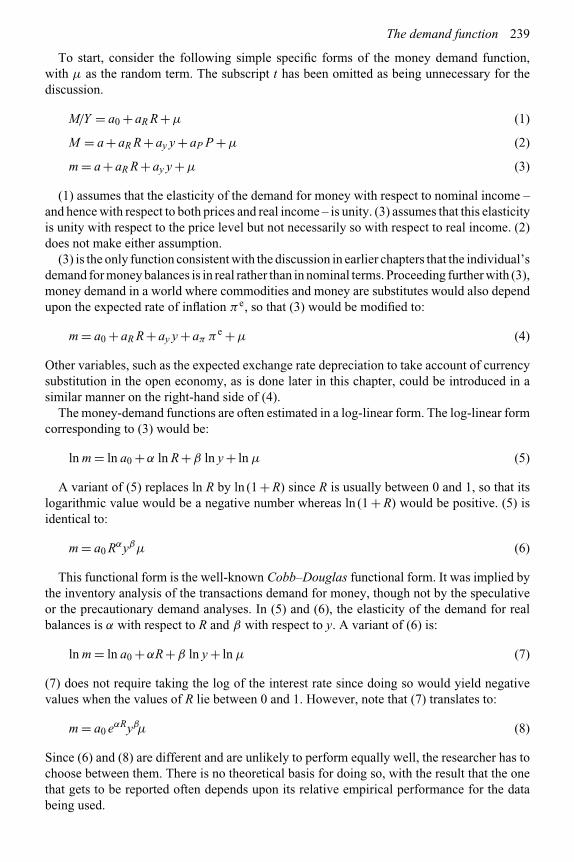
The demand function 239
To start, consider the following simple specific forms of the money demand function,with μ as the random term. The subscript t has been omitted as being unnecessary for thediscussion.
M/Y = a0 + aR R +μ (1)
M = a + aR R + ay y + aP P +μ (2)
m = a + aR R + ay y +μ (3)
(1) assumes that the elasticity of the demand for money with respect to nominal income –and hence with respect to both prices and real income – is unity. (3) assumes that this elasticityis unity with respect to the price level but not necessarily so with respect to real income. (2)does not make either assumption.
(3) is the only function consistent with the discussion in earlier chapters that the individual’sdemand for money balances is in real rather than in nominal terms. Proceeding further with (3),money demand in a world where commodities and money are substitutes would also dependupon the expected rate of inflation πe, so that (3) would be modified to:
m = a0 + aR R + ay y + aπ πe +μ (4)
Other variables, such as the expected exchange rate depreciation to take account of currencysubstitution in the open economy, as is done later in this chapter, could be introduced in asimilar manner on the right-hand side of (4).
The money-demand functions are often estimated in a log-linear form. The log-linear formcorresponding to (3) would be:
ln m = ln a0 +α ln R +β ln y + ln μ (5)
A variant of (5) replaces ln R by ln (1 + R) since R is usually between 0 and 1, so that itslogarithmic value would be a negative number whereas ln (1 + R) would be positive. (5) isidentical to:
m = a0 Rαyβμ (6)
This functional form is the well-known Cobb–Douglas functional form. It was implied bythe inventory analysis of the transactions demand for money, though not by the speculativeor the precautionary demand analyses. In (5) and (6), the elasticity of the demand for realbalances is α with respect to R and β with respect to y. A variant of (6) is:
ln m = ln a0 +αR +β ln y + ln μ (7)
(7) does not require taking the log of the interest rate since doing so would yield negativevalues when the values of R lie between 0 and 1. However, note that (7) translates to:
m = a0 eαRyβμ (8)
Since (6) and (8) are different and are unlikely to perform equally well, the researcher has tochoose between them. There is no theoretical basis for doing so, with the result that the onethat gets to be reported often depends upon its relative empirical performance for the databeing used.

240 The demand for money
8.1.1 Scale variable in the money demand function
Current income as the scale variable
The linear form of the demand function for real balances, with current income as the scalevariable, is:
mdt = a0 + ayyt + aRRt +μt a0,ay > 0,aR < 0 (9)
where μ is the random disturbance. (9) would become log-linear if each of the variables andμt were in logs.
Expected income as the scale variable
Another money demand function that is in common usage replaces current income byexpected income. A demand function with expected income as its scale argument is:
mdt = a0 + ayye
t + aRRt +μt a0,ay > 0,aR < 0 (10)
In (10), at the beginning of the period, mdt are the planned real balances for the period
ahead, yet is the expected income for the period. While we could have also introduced the
interest rate in terms of its expected value, this is rarely done. The current practice is toestimate expected income ye
t using the rational expectations hypothesis (REH).
Permanent income as the scale variable
As against current or expected income, Friedman’s (1956) theoretical analysis of the demandfor money presented in Chapter 2 implied that this demand depends upon wealth, or itsproxy, permanent income, and on interest rates. For Friedman’s analysis, the basic form ofthe demand function for real balances with permanent income is:
mdt = md(yp
t,Rt)
where ypt is permanent income, which can be interpreted as the average expected income
over the future. The simplified linear (or log-linear) form of this demand function for realbalances is:
mdt = a0 + ayyp
t + aRRt +μt a0,ay > 0,ar < 0 (11)
Since data on the observed values of ypt does not normally exist, Friedman used the adaptive
expectations hypothesis for deriving permanent income. Though the REH can be used asan alternative procedure for doing so, adaptive expectations seem more appropriate forestimating permanent income since the latter is best interpreted as the average expected valueof income, rather than merely as expected income for the period ahead. Correspondingly,md
t in (11) should be interpreted as the average expected amount of desired real balances.The adaptive expectations procedure for constructing permanent income is explained inSection 8.3.
Note that the three scale variables in (9) to (11) are different, so that their estimation willyield different coefficients. Further, even their stability properties may differ. As discussed

The demand function 241
later in this chapter and in Chapter 9, the time series for several variables, including money andincome, tend not to be stationary. The appropriate technique for such variables is cointegrationanalysis, which is a maximum likelihood vector autoregressive (VAR) technique. Suchestimation ignores altogether the distinction between expected and permanent income, sothat the prior application of the rational and adaptive expectations procedures is not neededif the money demand function is estimated using cointegration techniques. However, itsaccompanying error-correction estimation does incorporate adjustment lags and adaptiveexpectations.
8.2 Rational expectations
8.2.1 Theory of rational expectations
The rational expectations hypothesis (REH), first proposed by Muth (1961), is stated invarious forms. One way of stating it is that the individual uses all the available information athis disposal in forming his expectations on the future values of a variable. Since individualsoften have to – or choose to – operate with very limited information, the relevant informationset is sometimes specified to be one of maximizing profit. In any case, the availableinformation set is assumed to include the knowledge of the relevant theory,2 with therationally expected value of the variable being its value as predicted by this theory. The REHasserts that deviations of the actual from the theoretically predicted value will be randomlydistributed with a zero mean and be uncorrelated with the available information and with thetheoretically predicted value.
Note that the relevant theory will commonly determine the non-random prediction of avariable as a function of the parameters, the past values of the endogenous variables andthe past, current and future values of the exogenous variables. Of these, the future valuesof the exogenous variables will usually not be known to the individual and their rationalexpectations values will be needed, so that the relevant theory for them will also have tobe specified. In practical terms, the REH can be restated as: the expected values of theendogenous variables will be those predicted by the relevant theory, given the data on thepast values of the endogenous variables, those on the past and current values of the relevantexogenous variables, and the rationally expected future values of the relevant exogenousvariables.
Designate the rationally expected value of yet predicted by the relevant theory as yT
t ,where the superscript T stands for the relevant theory. Since yT
t takes account of all theinformation available to the individual, the REH asserts that the deviation of the actualvalue yt from yT
t will be random with a zero expected value and will be uncorrelatedwith the available information and, therefore, with yT
t which is based on that information.The following incorporates the above statements in a set of simple equations to show
2 The switch from “information available to the individual” to “knowledge of the relevant theory” is a massiveleap. The former implies a “subjective theory,” which is likely to differ from those held by others, whereas thelatter relates to an “objective theory” common to all individuals and based on accurate knowledge.
Note also that the word “relevant” is a loaded one. It means the correct theory for the economy or market inquestion. However, the correct theory is hardly ever known, as witnessed by the differing macroeconomic schoolson the determination of national income and inflation or by disagreements even among the exponents of a givenschool on the actual values of the structural and reduced form coefficients of the model.

242 The demand for money
the various assumptions and steps in deriving the rationally expected value ye∗t of the
variable yt .Since the rationally expected value ye∗
t – with e* standing for the rationally expectedvalue – is assumed to be determined by the value yT
t predicted by the relevant theory T, wehave:
ye∗t = yT
t (12)
Since the REH assumes that the actual value yt differs from the prediction of the relevanttheory T by an error that is random and not correlated with any available information, wehave:
yt = yTt +ηt (13)
where:
Eηt = 0 (14)
ρ(yTt,ηt) = 0 (15)
yt = actual income
yet = expected income
ye∗t = rationally expected value of income
yTt = expected income predicted by the relevant theory
Eηt = mathematical expectation of ηt
ρ(yTt,ηt) = correlation coefficient between yT
t and ηt .
(12) and (13) imply that:
yt = ye∗t +ηt (16)
Taking the mathematical expectation of (16), with Eηt = 0 from (14), and using (12) gives:
Eye∗t = Eyt = yT
t (17)
If ye∗t and yT are assumed, as is often done, to be single valued, (17) becomes:
ye∗t = Eyt = yT
t (18)3
To implement (18) empirically, the rationally expected value ye∗t can be obtained by
estimating yt using the function implied by the theory for its determination, and taking itsexpected value Eyt .4 This procedure is illustrated below and will also be applied in Chapter 17in a macroeconomics context.
3 This is called the weak version of the REH. A strong version of it is that F(ye∗t ) = f (yt ), where F and f specify
the respective frequency distributions. This version requires that the distribution of expected income is the sameas that of actual income except for a random term.
4 In purely theoretical analysis, yT is used for deriving ye∗ if yT is single valued. If it is not, ye∗ is replacedby EyT.
The demand function 243
The “relevant theory”
A fundamental question in applying the REH is about the definition of the term “relevanttheory.” To an economist who believes that the economy tends to be at full employment,even though it is currently not in that state, the relevant theory for forming expectations onaggregate output is that the economy will be at the full-employment level. Consequently, thefull-employment output will be the rationally expected one, so that the appropriate procedurewould be to solve the model or theory for its full-employment state and substitute it forthe expected output or real income. This procedure is the one adopted by economists in themodern classical approach.
However, for economists who believe that the economy is rarely, if ever, exactly in fullemployment, the rational expectation of next period’s real income will not be one of fullemployment. The theory needed for their rational expectations of income would be a theoryof the non-random part of the expected level of actual income, since this is the level thatwould differ from next period’s actual income by a random term. Keynesian economistsfollow this line of thinking and need to specify a theory of the expected value of actual outputfor the period in question.
Hence, the application of the REH will yield different values of rationally expected output,depending upon the underlying assumption of the continuous existence or frequent absence offull employment. While the REH at the conceptual level can be and is used by both classicaland Keynesian economics, its application, even in the context of an otherwise identical model(e.g. the IS–LM one), provides different predictions of the expected future income for thetwo approaches.
To proceed further, (18) can be used to construct the estimate of ye∗t by using the
relevant theory to specify the determination of yTt . We illustrate this use of the theory
by incorporating two alternative theories on the relationship between output and the rateof increase in the money supply. The first theory will be the Lucas supply rule, whichunderpins modern classical macroeconomics, and the second one will be the Keynesiantheory.5
8.2.2 Information requirements of rational expectations: an aside
There is considerable dispute in the literature about the information requirements for rationalexpectations. The information available to any given individual varies considerably, interalia, with the individual’s level of education and interest, the openness of the society and theoperating technology of information, as well as the losses from basing actions on inadequate,vague and inaccurate information. The actual amount of information at the disposal of theindividual can vary from almost non-existent hard information6 to extensive knowledge. TheREH is meant to apply to all cases, regardless of the extent and accuracy of the availableinformation.
Skeptics about the REH have argued that it requires that the possible future outcomesare well anticipated and that economic agents are assumed to be superior economists and
5 See Chapters 15 and 17 for these models and rules.6 For instance, in many underdeveloped or developing countries there is hardly any reliable information published
on national income and the rate of inflation. Even if it is published, most of the inhabitants in the rural and eventhe urban areas may never receive or bother to acquire this information.
244 The demand for money
statisticians, capable of analyzing the future general equilibrium of the economy (Arrow,1978). However, the supporters of rational expectations reject such criticism and claim that:
The implication that economic agents or economists are omniscient cannot fairly bedrawn from Muth’s profound insights. … Rational expectations are profit maximizingexpectations. … If the past proves to be a very imperfect guide to the future, then theoryand practice will be inaccurate.
(Kantor, 1979, p. 1424).
It is, however, incorrect to assume that rational expectations regards errors as insignificantor absent. The implication of rational expectations is that the forecast errors are notcorrelated with anything that could profitably be known when the forecast is made.
(Kantor, 1979, p.1432).
Another view of rational expectations is provided by Robert Lucas, who popularized itsusage in macroeconomics. The Economist website reported that Lucas at one time said that:
[Rational expectations] doesn’t describe the actual process people use trying to figure outthe future. Our behavior is adaptive. We try some mode of behavior, if it is successful,we do it again. If not, we try something else. Rational expectations describe the situationwhen you’ve got it right.7
This interpretation means that, for most of the time spent in figuring out the future andacting on one’s expectations, we would not have rational expectations with its criticalproperty that the errors between the actual and the expected value would be random.Since rational expectations will only hold eventually (“when you have got it right”), theyshould be restricted only to the long-run analysis. They will not apply over short periodsand in the short run. This interpretation of rational expectations is not consistent withthe macroeconomic literature on it, including Lucas’s own contributions on the short-runmacroeconomic model. It is also not consistent with the use and analyses of the Lucassupply rule presented in this chapter and in Chapter 14. We shall henceforth ignore thisinterpretation.
Assessing the validity of the rational expectations hypothesis
The insight behind rational expectations at its conceptual level – that is, when an individual’sexpectations are based on all his available information – is undeniable. However, part of theavailable information comes from our understanding of the past and the present, which isitself incomplete and imperfect, as witnessed by the prevalence, even in hindsight, of differenttheories to explain any given observation. In addition, knowledge of the future is even moreuncertain; as the quote at the end of this subsection argues, for the future, we don’t even knowwhat we don’t know. Given the increasing increment of this degree of ignorance for periodsfurther ahead, short-term (i.e. for the next quarter or so) predictions tend to do better than forperiods further ahead. But, for these, the persistence forecast (i.e. the immediate future will
7 http://economistsview.typepad.com/economistsview/2007/09/expect-the-unexp.html, downloaded and printed 12September 2007.
The demand function 245
be like the immediate past except for random variations) does quite well – and usually betterthan predictions based on any theory.
In the rational expectations hypothesis, the leap from the “subjective/personal theory”based on the available information to the assumption of the “relevant theory,” common toall individuals as well as being the accurate theory, is a massive one. This assumption is alsolikely to be invalid. The exponents of the REH, with Kantor among them, focus on the former,whereas its critics, with Arrow among them, focus on the latter. Leaving aside the doctrinaldisputes, the empirical issue boils down to a question of the usefulness or profitability ofacting on one’s rational expectations. This usefulness can be extremely limited when –without knowledge of the relevant theory and without good reliable information on the pastvalues of the endogenous and exogenous variables, or on the relevant future values of theexogenous variables – the known paucity of information indicates that the actual error inthe rationally expected value of a variable can be large8 relative to the mean expected valueof the variable, so that acting on the basis of the rationally expected value of the variablemay not turn out to be a prudent exercise.9 Conversely, if the information available is quitecomplete and the subjective probabilities are known to approximate the objective ones, therational expectations could be an appropriate basis for action.
An interesting take on the nature of uncertainty and how it limits the reliability andusefulness of rational expectations for decisions is provided by the following quote:
There are things that we know. There are [also] known unknowns; that is to say that thereare things we now know that we don’t know. But there are also unknown unknowns –things that we do not know we don’t know. So when we do the best we can and we pullall the information together, and we then say, “Well, that is basically what we see as thesituation,” that is really only the known knowns and the known unknowns. And [as timepasses] we discover a few more of those unknown unknowns. There is another way tophrase that, and that is that the absence of evidence is not evidence of absence.
(Donald Rumsfeld in a news conference, June 2002; italics added).
8.2.3 Using the REH and the Lucas supply rule for predicting expected income
This rule assumes the modern classical model, with the labor market being in long-runequilibrium at full employment and with deviations in real national output from its fullemployment level yf occurring only due to errors in predicting the actual level of the
8 This need not mean that their mean value is not zero. It is that they can take relatively large absolute values.9 Acting on the basis of the same rationally expected value of a variable may be very prudent behavior when the
information on which it is based is fairly complete and reliable. Acting on it may be foolhardy behavior when theinformation is scanty and represents a shot in the dark rather than an adequate basis for action.
A distinction is drawn here between “prudence” and “profit maximizing” in the presence of an acute lack ofinformation; I may know nothing about horse racing and about the horses entered in a race, yet I can on the basisof the available information – say on the pleasing and non-pleasing colors of horses – specify my subjectiveprobabilities of the performance of the horses in the race and place my profit-maximizing bets on the basis ofthese probabilities. Prudence may instead dictate that I recognize the vagueness and inadequacy of my informationunderlying my probabilities and that I do not bet at all.
Another distinction is drawn between holding rational expectations and acting on those expectations. Rationalexpectations can always be held, as long as the required probabilities are subjective and not objective ones.However, experience may have taught the individual not to act on them, or to act on them after due allowanceand caution for a large margin of uncertainty, ambiguity and error.
246 The demand for money
money supply. One form of the Lucas supply rule10 specifies the relevant theory for thedetermination of output y in period t as:
yTt = yf
t + γ (Mt − M et) (19)
where:yf
t = full employment level of output in tMt = nominal money stock in t
M et = expected value of the nominal money stock in t
M e∗t = rational expectations of Mt , formed in t −1
so that the rational expectation of income, with the Lucas supply rule as the relevant theoryfor its determination, is:
ye∗t = yf
t + γ (Mt − M e∗t) (20)
Use of (20) for predicting rationally expected income requires using the relevant theoryto determine M e∗
t . The relevant theory depends upon the monetary policy being pursued bythe monetary authority.11 In the context of an exogenous money supply, the central bankcontrols the money supply and can determine the money supply in the economy on the basisof a “rule” or function. Assume this to be the case, and that the relevant theory for the centralbank’s money supply rule MT is:
MTt = Ψ0 +Ψ1ut−1 +Ψ2Mt−1 (21)
where ut is the unemployment rate (or the output gap between full employment and actualoutput) in period t. Designating the random error in Mt as ξ t , (21) leads to the specificationof Mt as:
Mt = Ψ0 +Ψ1ut−1 +Ψ2Mt−1 + ξt (22)
Estimating (22) will provide the estimated values of the coefficients Ψi, i = 0,1,2, as Ψ .These estimated coefficients can be used to estimate EMt , which yields the rationally expectedvalue M e∗
t , as:
M e∗t = EMt
= Ψ0 + Ψ1ut−1 + Ψ2Mt−1 (23)
Since Mt − M e∗t = Mt − Ψ0 + Ψ1ut−1 + Ψ2Mt−1 = ξt , where ξt is the estimated value of ξt ,
(19) implies that:
yt = yft + γ ξt +ηt (24)12
10 The macroeconomics of the Lucas supply rule are covered in Chapter 14. This rule makes the output gap(yt − yf
t ) a positive function of the deviation of the price level from its expected value. Adding the assumptionthat the price level is a function of the money supply leads to the specification of the Lucas supply rule assumedin the text.
Note that the Lucas supply rule is not consistent with the various specifications of the Keynesian model.11 See Chapters 10, 11, 13 and 17 for the money supply theories.12 ξt is the estimated value of the unanticipated money supply obtained from the estimation of (22).
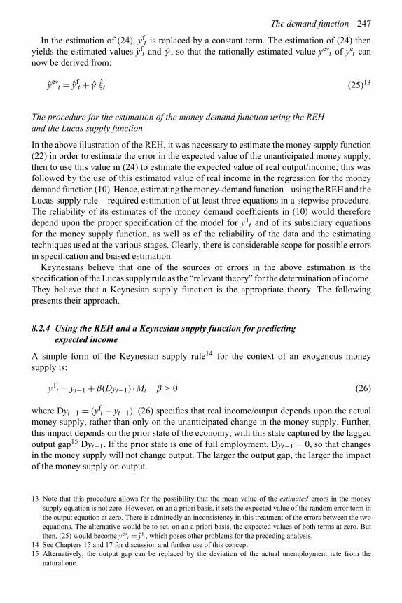
The demand function 247
In the estimation of (24), yft is replaced by a constant term. The estimation of (24) then
yields the estimated values yft and γ , so that the rationally estimated value ye∗
t of yet can
now be derived from:
ye∗t = yf
t + γ ξt (25)13
The procedure for the estimation of the money demand function using the REHand the Lucas supply function
In the above illustration of the REH, it was necessary to estimate the money supply function(22) in order to estimate the error in the expected value of the unanticipated money supply;then to use this value in (24) to estimate the expected value of real output/income; this wasfollowed by the use of this estimated value of real income in the regression for the moneydemand function (10). Hence, estimating the money-demand function – using the REH and theLucas supply rule – required estimation of at least three equations in a stepwise procedure.The reliability of its estimates of the money demand coefficients in (10) would thereforedepend upon the proper specification of the model for yT
t and of its subsidiary equationsfor the money supply function, as well as of the reliability of the data and the estimatingtechniques used at the various stages. Clearly, there is considerable scope for possible errorsin specification and biased estimation.
Keynesians believe that one of the sources of errors in the above estimation is thespecification of the Lucas supply rule as the “relevant theory” for the determination of income.They believe that a Keynesian supply function is the appropriate theory. The followingpresents their approach.
8.2.4 Using the REH and a Keynesian supply function for predictingexpected income
A simple form of the Keynesian supply rule14 for the context of an exogenous moneysupply is:
yTt = yt−1 +β(Dyt−1) · Mt β ≥ 0 (26)
where Dyt−1 = (yft − yt−1). (26) specifies that real income/output depends upon the actual
money supply, rather than only on the unanticipated change in the money supply. Further,this impact depends on the prior state of the economy, with this state captured by the laggedoutput gap15 Dyt−1. If the prior state is one of full employment, Dyt−1 = 0, so that changesin the money supply will not change output. The larger the output gap, the larger the impactof the money supply on output.
13 Note that this procedure allows for the possibility that the mean value of the estimated errors in the moneysupply equation is not zero. However, on an a priori basis, it sets the expected value of the random error term inthe output equation at zero. There is admittedly an inconsistency in this treatment of the errors between the twoequations. The alternative would be to set, on an a priori basis, the expected values of both terms at zero. Butthen, (25) would become ye∗
t = yft , which poses other problems for the preceding analysis.
14 See Chapters 15 and 17 for discussion and further use of this concept.15 Alternatively, the output gap can be replaced by the deviation of the actual unemployment rate from the
natural one.
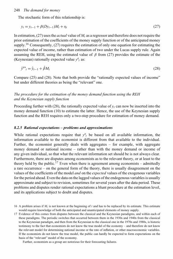
248 The demand for money
The stochastic form of this relationship is:
yt = yt−1 +β(Dyt−1)Mt +ηt (27)
In estimation, (27) uses the actual value of Mt as a regressor and therefore does not require theprior estimation of the coefficients of the money supply function or of the anticipated moneysupply.16 Consequently, (27) requires the estimation of only one equation for estimating theexpected value of income, rather than estimation of two under the Lucas supply rule. Againassuming the REH, using the estimated value of β from (27) provides the estimate of the(Keynesian) rationally expected value ye
t as:
ye∗t = yt−1 + βMt (28)
Compare (25) and (28). Note that both provide the “rationally expected values of income”but under different theories as being the “relevant” one.
The procedure for the estimation of the money demand function using the REHand the Keynesian supply function
Proceeding further with (28), the rationally expected value of yt can now be inserted into themoney demand function (10) to estimate the latter. Hence, the use of the Keynesian supplyfunction and the REH requires only a two-step procedure for estimation of money demand.
8.2.5 Rational expectations – problems and approximations
While rational expectations require that yet be based on all available information, the
information available to the economist is different from that available to the individual.Further, the economist generally deals with aggregates – for example, with aggregatemoney demand or national income – rather than with the money demand or income ofany given individual, so that what the relevant information set should be is not always clear.Furthermore, there are disputes among economists as to the relevant theory, or at least to thetheory held by the public.17 Even when there is agreement among economists – admittedlya rare occurrence – on the general form of the theory, there is usually disagreement on thevalues of the coefficients of the model and on the expected values of the exogenous variablesfor the period ahead. Even the data on the lagged values of the endogenous variables is usuallyapproximate and subject to revision, sometimes for several years after the data period. Theseproblems and disputes render rational expectations a blunt procedure at the estimation level,and its applications subject to doubt and disputes.
16 A problem arises if Mt is not known at the beginning of t and has to be replaced by its estimate. This estimatewould require knowledge of both the anticipated and unanticipated elements of money supply.
17 Evidence of this comes from disputes between the classical and the Keynesian paradigms, and within each ofthese paradigms. The periodic switches that occurred between them in the 1930s and 1940s from the classicalto the Keynesian paradigm, and then from the Keynesian to the classical one in the 1970s and 1980s, is historictestimony to the fact that economists do not know the true model of the economy – and therefore do not knowthe relevant model for determining national income or the rate of inflation, or other macroeconomic variables.If the economists do not know the true model, the public can hardly be expected to form expectations on thebasis of the “relevant” model of the economy.
Further, economists as a group are notorious for their forecasting failures.
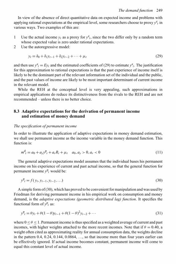
The demand function 249
In view of the absence of direct quantitative data on expected income and problems withapplying rational expectations at the empirical level, some researchers choose to proxy ye
t invarious ways. Two examples of this are:
1 Use the actual income yt as a proxy for yet , since the two differ only by a random term
whose expected value is zero under rational expectations.2 Use the autoregressive model:
yt = δ0 + δ1yt−1 + δ2yt−2 +·· ·+μt (29)
and then use yet = Eyt and the estimated coefficients of (29) to estimate ye
t . The justificationfor this approximation to rational expectations is that the past experience of income itself islikely to be the dominant part of the relevant information set of the individual and the public,and the past values of income are likely to be most important determinant of current incomein the relevant model.
While the REH at the conceptual level is very appealing, such approximations inempirical applications do reduce its distinctiveness from the rivals to the REH and are notrecommended – unless there is no better choice.
8.3 Adaptive expectations for the derivation of permanent incomeand estimation of money demand
The specification of permanent income
In order to illustrate the application of adaptive expectations in money demand estimation,we shall use permanent income as the income variable in the money demand function. Thisfunction is:
mdt = a0 + ayyp
t + arRt +μt a0,ay > 0,ar < 0 (11)
The general adaptive expectations model assumes that the individual bases his permanentincome on his experience of current and past actual income, so that the general function forpermanent income yp
t would be:
ypt = f ( yt,yt−1,yt−2, . . .) (30)
A simple form of (30), which has proved to be convenient for manipulation and was used byFriedman for deriving permanent income in his empirical work on consumption and moneydemand, is the adaptive expectations (geometric distributed lag) function. It specifies thefunctional form of yp
t as:
ypt = θyt + θ (1 − θ )yt−1 + θ (1 − θ )2yt−2 +·· · (31)
where 0 ≤ θ ≤ 1. Permanent income is thus specified as a weighted average of current and pastincomes, with higher weights attached to the more recent incomes. Note that if θ = 0.40, aweight often cited as approximating reality for annual consumption data, the weights declinein the pattern 0.4, 0.24, 0.144, 0.0864, …, so that income more than four years earlier canbe effectively ignored. If actual income becomes constant, permanent income will come toequal this constant level of actual income.

250 The demand for money
Koyck transformation of the geometric distributed lag function
Lag (31) one period and multiply each term in it by (1 − θ ). This gives:
(1 − θ )ypt−1 = θ (1 − θ )yt−1 + θ (1 − θ )2yt−2 + θ (1 − θ )3yt−3 +·· · (32)
Subtracting (32) from (31) gives the equation:
ypt = θyt + (1 − θ )yp
t−1 (33)
(33) is known as the Koyck transformation. This transformation allows permanent incometo be stated in terms of the revision of its value last period in the light of current income.
Deriving the estimation form of the money demand function
Substituting ypt from (33) in the money demand function (11) gives:
mdt = a0 + ayθyt + ay(1 − θ )yp
t−1 + aRRt +μt (34)
Lag each term in (34) by one period and multiply it by (1 − θ ). This gives:
(1 − θ )mdt−1 = (1 − θ )a0 + ay(1 − θ )yp
t−1 + aR(1 − θ )Rt−1 + (1 − θ )μt−1 (35)
Subtracting (35) from (34) to eliminate ypt−1 gives:
mdt = a0θ + ayθyt + aRRt − aR(1 − θ )Rt−1 + (1 − θ )md
t−1 +{μt − (1 − θ )μt−1} (36)
where ay,aR > 0, and 0 ≤ θ ≤ 1. The objective in carrying out the above steps was to eliminatethe variable yp on which data is not available. (36) achieves this objective.
The estimating form of (36) is:
mdt = α0 +α1yt +α2Rt +α3Rt−1 +α4md
t−1 +ηt (37)
where:α0 = a0θ
α1 = ayθ
α2 = aR
α3 = −aR(1 − θ )α4 = (1 − θ )ηt = {μt − (1 − θ )μt−1}
Note that (37) involves lagged terms in m and in R, but not in y. Further, the disturbance termin (37) is {μt + (1 − θ )μt−1}, which is a moving average error.
Adaptive expectations as the error-learning model
The adaptive expectations procedure in the form given by (33) can also be stated in a formknown as the error-learning model. This form is:
(ypt − yp
t−1) = θ (yt − ypt−1) (38)

The demand function 251
which specifies the revision in permanent income on the basis of the experienced differenceor “error” between the actual income in t and the permanent income for period (t − 1).From (38), if θ = 0, the estimate of permanent income is never revised on the basis of theexperience of current income.
Assessing the relevance and validity of the adaptive expectations procedure
If we compare the rational and the adaptive expectations procedures for estimating themoney-demand function, the former requires the estimation of at least two (possibly three,as in our illustration above) equations for the Lucas supply rule. However, doing so hasthe advantage that it allows better identification of the sources of shifts. Conversely, theadaptive expectations procedure has the disadvantage that if the parameters of the estimatedmoney demand function shift, it is not clear whether the parameters of the money demandfunction or of the expected income equation have shifted. Further, in cases of monotonicallyincreasing (decreasing) income paths, adaptive expectations induce persistent and increasingnegative (positive) errors (i.e. yt − yp
t) in expected income relative to actual income, sothat rational individuals will revise their procedure for forming expectations away fromadaptive expectations. Adaptive expectations also fail to take account of any informationavailable to the individual about future changes in income, and are said to be (only) backwardlooking.
However, note that the adaptive expectations model, in spite of its name, really providesan estimate of the average level of future income – rather than the expected value ofincome for the period ahead – through its geometric distributed lag procedure, while theREH procedure provides a more appropriate estimate of the latter. The two procedurestherefore provide proxies for different concepts of income, so that the choice among themshould depend on the income variable, which is the appropriate scale variable in the moneydemand function. If the non-stochastic component of income is fluctuating and the appropriatescale variable is permanent or average expected income yp
t , the geometric distributed lagwould be a better representation of this average than the rationally expected value of currentincome ye∗
t .18
8.4 Regressive and extrapolative expectations
An alternative to adaptive expectations is the regressive expectations model, whichspecifies that:
yet = yt−1 + δ( yLR − yt−1) (39)
where yLR is the long-run level of income. Here, the expectation is that income will tendtowards its long-run value.19
Another model of expectations is the extrapolative expectations one. It is that:
yet − yt−1 = δ( yt−1 − yt−2) (40)
18 However, the rationally expected value of a permanent measure of future incomes would be better still.19 Keynes specified such a process for interest rate expectations in the speculative demand for money: the individual
expects the interest rate to move towards its long-run value.

252 The demand for money
This model assumes that income is expected to change as a proportion of the change inincome in the preceding period. That is, recent changes – or the factors producing thosechanges – are expected to determine the pattern of future changes.
Whether the adaptive, regressive, extrapolative or rational expectations procedures aremore appropriate depends upon how the individual forms his expectations. The adaptiveexpectations model seems to be the most common one for modeling permanent income, i.e.average expected income, while the rational expectations procedure is the most common onefor modeling expected income over the period ahead.
8.5 Lags in adjustment and the costs of changing money balances
Lags often occur in the adjustment of money demand to its desired long-run value. Therecan be several reasons for such lags. Among these are: (i) habit persistence and inertia,(ii) slow adjustment of money balances due to uncertainty on whether the changes in thedeterminants (income and interest rates) of money demand are transitory or longer lasting,and (iii) adjustment costs, which can be monetary or non-monetary. This section focuseson adjustment costs and presents the derivation of adjustment patterns from adjustment costfunctions.
First-order partial adjustment model
One reason for an adjustment lag can be the short-run cost of changing money balances. Toinvestigate the relationship between such costs and the adjustment lag in money balances,let the individual’s desired real balances be m∗
t and assume that the individual faces varioustypes of costs of adjusting instantaneously to m∗
t . Examples of such costs are:
(i) The cost of being below or above m∗t . For example, having inadequate balances can
prevent one from carrying out purchases which require immediate payments in money.(ii) The cost of changing actual balances from mt−1 to mt .
These costs can take various forms. A simple form of these occurs when (i) has theproportional quadratic form a(mt − m∗
t)2 and (ii) has the proportional quadratic formb(mt − mt−1)2. Assuming these to be so, the total adjustment cost c of reaching the desiredbalance in period t is given by:
ct = a(mt − m∗t)
2 + b(mt − mt−1)2 a,b ≥ 0 (41)
The individual is taken to minimize this cost. The first-order condition for maximization isthat:
∂ct/∂mt = 2a(mt − m∗t) + 2b(mt − mt−1) = 0 (42)
which yields the actual balances mt as:
mt = γ m∗t + (1 − γ )mt−1 (43)
where γ = a/(a + b). (43) can be restated in a more intuitive form as:
mt − mt−1 = γ (m∗t − mt−1) 0 ≤ γ ≤ 1 (44)

The demand function 253
(43) and (44) constitute the first-order (i.e. with a one-period lag only) partial adjustmentmodel (PAM ): the adjustment of real balances in period t is partial, linear and involvesa one-period lag. This model suffers from the disadvantage that if m*t has a positive ornegative trend, the divergence of actual balances from the desired ones will increase overtime. Individuals would find it profitable to avoid this by abandoning the first-order PAM andusing some other adjustment mechanism.20 Therefore, the first-order PAM is inappropriatewhen the desired or actual balances have a strong trend component.21 A higher-level PAMwould be more appropriate in such a case.22
Second-order partial adjustment model
Higher-order partial adjustment models result from more complicated specifications of theadjustment costs. The second-order (i.e. with a two-period) partial adjustment model is givenby the adjustment cost function:
ct = a(mt − m∗t)
2 + b(mt − mt−1)2 + k(�mt −�mt−1)2 a,b,k > 0 (45)
= a(mt − m∗t)
2 + b(mt − mt−1)2 + k(mt − 2mt−1 + mt−2)2 (46)
where �mt = mt −mt−1, and k(�mt −�mt−1)2 is additional to the adjustment costs (i) and(ii) and represents the cost of continual adjustments over time in balances. Minimizing (46) –that is, setting the partial derivative of c with respect to m equal to zero – and solving impliesthat:
mt = γ1m∗t + γ2mt−1 + (1 − γ1 − γ2)mt−2 (47)
where:γ1 = a/(a + b + k)γ2 = (b + 2k)/(a + b + k)
Since (47) has a two-period lag, it provides the second-order partial adjustment model.
Error feedback model
A further elaboration of these models is obtained if, in addition to the earlier types of costs,the costs of continual adjustment were less when the actual changes �mt were in the samedirection as the desired changes �m∗
t . A specification of such a cost function would be:
ct = a(mt − m∗t)
2 + b(mt − mt−1)2 − k�m∗t(mt − mt−1) a,b,k > 0 (48)
20 From a rational expectations perspective, partial adjustment models are inappropriate since they are backwardlooking and do not take account of the available information on the expected future changes in desired balances.The individual may find it profitable to make changes in current balances to provide for future changes in desiredbalances.
21 The first-order PAM imposes the same response pattern to the changes in desired balances, irrespective ofwhether such a change is due to changes in income or in interest rates. In fact, the adjustment costs may differdepending upon the source of the changes in the desired balances.
22 This is desirable to detrending the data and using the first-order PAM.

254 The demand for money
In this case, the demand for actual balances would be:
mt = mt−1 + γ1(m∗t − mt−1) + γ2(m∗
t − m∗t−1) (49)
where γ1 = [a/(a+b)] and γ2 = [k/{2(a+b)}]. (49) is another form of PAM and is the errorfeedback model.
Assessing the validity of partial adjustment models
The various types of adjustment cost functions depend upon the notion that it is costly for theindividual to change money balances. As in the inventory model of transactions balances inChapter 4, this cost is the sum of both monetary and non-monetary costs and will differ for thedifferent definitions of money. In practice, in modern financially developed economies withinternet banking, the costs of converting to M1 from savings deposits and other near-moneyassets have become virtually zero, so that there should not be any significant adjustmentlags at the level of the individual. The costs of changing M2 can be similarly very smalland may be of little consequence at the individual’s level. This is especially so when suchcosts are compared with those of changing the individual’s stock of commodities or laborsupplied.23 The costs of adjustment for monetary aggregates usually become significant onlywhen such adjustment involves converting bonds or commodities into a monetary asset. Butthis happens rarely for meeting desired changes in the demand for M1 and M2, so that thepractice of using PAM models, especially for the narrower definition of money, may be ofquestionable value. However, the lagged adjustment implied by these models is part of theerror-correction modeling within the currently popular cointegration technique.
8.6 Money demand with the first-order PAM
If there exist adjustment costs in changing money holdings, these costs should properlybe incorporated into the structure of the individual’s decision processes and the demandfor money holdings be derived after such incorporation. However, this can prove to beanalytically intractable, so that the usual procedure is to derive the demand function separatelyfrom the adjustment function and then combine them. This is the procedure followed here.
Assume that the individual’s demand for real balances depends on current real income yand the nominal interest rate R, so that the demand function is:
m∗t = a0 + ayyt + aRRt +μt a0,ay > 0,aR < 0 (50)
where μ is white noise. m∗t are the desired real balances in the absence of adjustment costs.
Further, assume the first-order PAM, which is:
mt − mt−1 = γ (m∗t − mt−1) 0 ≤ γ ≤ 1 (44)
Substituting (44) into (50) to eliminate m*t gives:
mt = a0γ + ayγ yt + aRγ Rt + (1 − γ )mt−1 + γμt (51)
23 This idea was explored in Chapter 6 in the context of buffer stock models of money.
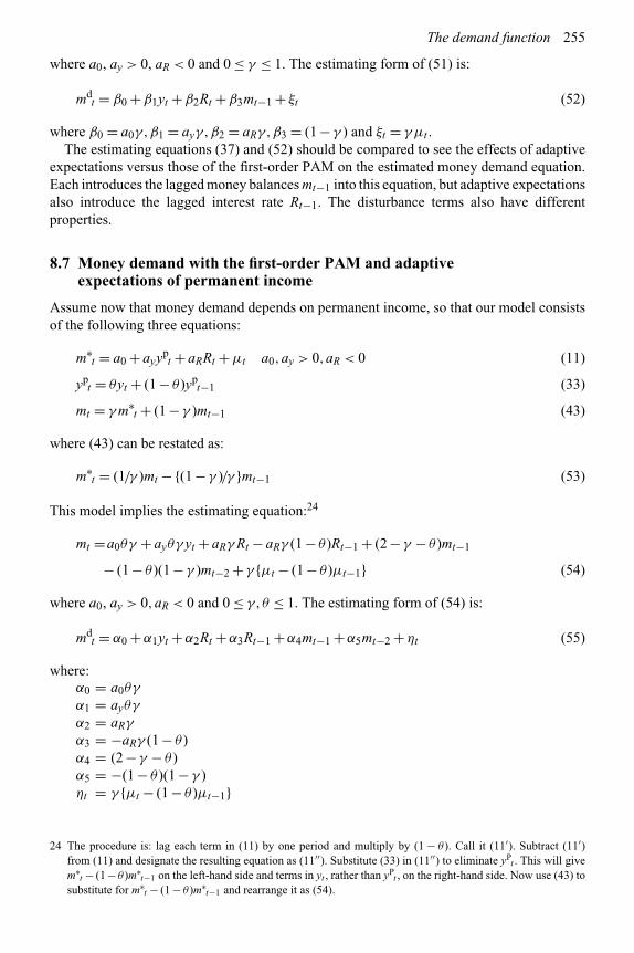
The demand function 255
where a0, ay > 0, aR < 0 and 0 ≤ γ ≤ 1. The estimating form of (51) is:
mdt = β0 +β1yt +β2Rt +β3mt−1 + ξt (52)
where β0 = a0γ,β1 = ayγ,β2 = aRγ,β3 = (1 − γ ) and ξt = γμt .The estimating equations (37) and (52) should be compared to see the effects of adaptive
expectations versus those of the first-order PAM on the estimated money demand equation.Each introduces the lagged money balances mt−1 into this equation, but adaptive expectationsalso introduce the lagged interest rate Rt−1. The disturbance terms also have differentproperties.
8.7 Money demand with the first-order PAM and adaptiveexpectations of permanent income
Assume now that money demand depends on permanent income, so that our model consistsof the following three equations:
m∗t = a0 + ayyp
t + aRRt +μt a0,ay > 0,aR < 0 (11)
ypt = θyt + (1 − θ )yp
t−1 (33)
mt = γ m∗t + (1 − γ )mt−1 (43)
where (43) can be restated as:
m∗t = (1/γ )mt −{(1 − γ )/γ }mt−1 (53)
This model implies the estimating equation:24
mt =a0θγ + ayθγ yt + aRγ Rt − aRγ (1 − θ )Rt−1 + (2 − γ − θ )mt−1
− (1 − θ )(1 − γ )mt−2 + γ {μt − (1 − θ )μt−1} (54)
where a0, ay > 0,aR < 0 and 0 ≤ γ,θ ≤ 1. The estimating form of (54) is:
mdt = α0 +α1yt +α2Rt +α3Rt−1 +α4mt−1 +α5mt−2 +ηt (55)
where:α0 = a0θγ
α1 = ayθγ
α2 = aRγ
α3 = −aRγ (1 − θ )α4 = (2 − γ − θ )α5 = −(1 − θ )(1 − γ )ηt = γ {μt − (1 − θ )μt−1}
24 The procedure is: lag each term in (11) by one period and multiply by (1 − θ ). Call it (11′). Subtract (11′)from (11) and designate the resulting equation as (11′′). Substitute (33) in (11′′) to eliminate yP
t . This will givem∗
t − (1− θ )m∗t−1 on the left-hand side and terms in yt , rather than yP
t , on the right-hand side. Now use (43) tosubstitute for m∗
t − (1 − θ )m∗t−1 and rearrange it as (54).

256 The demand for money
(55) provides a more general estimating equation than either the PAM model or the adaptiveexpectations model. These two models are therefore nested in (55), with the PAM one aloneobtained when θ = 1 and the adaptive expectations obtained when γ = 1. Hence (55) providesa way of testing whether there exist both or either of these processes. However, (55) is notnecessarily preferable to the alternative estimation procedure that uses the PAM and rationalexpectations to estimate expected income.
The structural coefficients in (54) are: a0, ay, aR, γ , θ . The coefficients in the estimatingequation (55) are: α0, …, α5. Hence, there are only five structural coefficients compared withsix coefficients in the estimated equation, so that appropriate non-linear restrictions have tobe imposed on the αi in the estimating equation (55).
The earlier criticisms of adaptive expectations from the rational expectations perspectivealso apply here. To reiterate, the criticism is that adaptive expectations are backward lookingand ignore information that may be available to the individual about the future as well ason other variables. Further, if the expectations parameter θ shifts, the estimating equation(55) would shift, without it being transparent whether the shift is due to a shift in γ , in θ , orin the coefficients of the demand function. By comparison, using the rational expectationsprocedures to estimate yp
t in the first step, and then estimating the demand function withPAM, will more clearly disclose the source of the shift in the money demand function.
8.8 Autoregressive distributed lag model: an introduction
Now suppose that the demand for real balances depends on the current and lagged values ofreal income and its own lagged values. That is, it has the form:
mt = a0yt + a1yt−1 + a2yt−2 +·· ·+ b1mt−1 + b2mt−2 +·· · (56)
This equation is the representation of the general autoregressive distributed lag (ARDL)model. yt−i can be replaced by Liyt , where Li is the lag operator, which can be treated as avariable subject to mathematical manipulation in the following manner:
a0yt + a1yt−1 + a2yt−2 +·· · = a0yt + a1Lyt + a2L2yt +·· ·= yt(a0 + a1L + a2L2 +·· ·)= a(L)yt (57)
where a(L) is the polynomial (a0 + a1L + a2L2 +·· · ) in L. Hence, (56) can be rewritten as:
mt = a(L)yt + b(L)mt (58)
where:
a(L) = a0 + a1L + a2L2 +·· ·b(L) = b1L + b2L2 +·· ·
Therefore,
mt − b(L)mt = a(L)yt
mt = [{1 − b(L)}−1 · a(L)]yt (59)

The demand function 257
so that mt becomes a function solely of yt and its lagged terms, without its own lagged values,which are now omitted from the explanatory terms. (59) is the compact form of the ARDLlag model.
An illustration: a simple ARDL model
As an illustration, consider the simplest example of (59) where a(L) = a0 and b(L) = b1L.That is, (56) is simplified to:
mt = ayyt + b1mt−1 (60)
In this case, (59) simplifies to:
mt = {1 − b1L}−1 · ayyt (61)
Expand {1−b1L}−1 in a Taylor’s series around E(b1L) = 0, where E(b1L) is the mean valueof b1L. This gives:
{1 − b1L}−1 = {1 + b1L + b2L2 +·· ·
Hence, (61) becomes:
mt = {1 + b1L + b2L2 +·· ·}ayyt (62)
= ayyt + ayb1yt−1 + ayb2yt−2 +·· · (63)
While (60) and (63) are mathematical transformations of each other, so that their economiccontent is identical, the money demand function in the form of (63) does not contain the laggedvalue of the endogenous variable, although we started with equation (60) where it does so.Conversely, we could have started with (63) without the lagged money term and derived(60) as equivalent to it. Hence a comparison of (60) and (63) – and of (59) with (56) forthe general case – leads to the caution that it may not be possible to distinguish between amoney demand equation which contains the lagged values of the endogenous variable andother independent variables, and one which contains only the current and lagged values ofthe independent variables.
The general ARDL model with the suitable addition of disturbance terms is now incommon usage in monetary analysis, and falls in the category of vector autoregression (VAR)models.25 Its relationship with the now popular cointegration and error-correction estimationis given in the appendix to Chapter 9.
8.9 Demand for money in the open economy
This book has so far concentrated on the demand for money in the closed economy. Thisis the general pattern of studies on money demand. However, economies are becoming
25 In some of the VAR models used in the analysis of monetary policy, the disturbance terms are interpreted andmodeled as policy initiatives, thereby allowing the dynamic intertemporal impact of various policy options tobe derived. This use of VAR models has made them fairly popular in the dynamic analysis of monetary policy.

258 The demand for money
increasingly open to flows of commodities and financial assets, so that a special topic in themoney demand literature deals with money demand in the open economy, in which economicunits have access not only to domestic financial assets but also to foreign ones.
For portfolio investments in open economies, the financial alternatives to holding domesticmoney include the currencies and bonds of foreign countries, in addition to domestic bonds,so that the determinants of the domestic money demand should include not only the rates ofreturn on domestic assets but also those on foreign assets. Since these assets include foreignmoney holdings, money demand studies for open economies need to pay special attention tosubstitution between domestic and foreign monies. This determination is especially relevantfor open economies in which foreign currencies are extensively traded and foreign moniesare part of the domestic media of payments. Note that the relevant literature on substitutionbetween domestic and foreign money in the open economy uses the word “currency” formoney. This chapter follows this usage.
Currency substitution (CS) can be defined as substitution between domestic and foreigncurrencies, which is “currency–currency substitution.” Substitution can also exist betweendomestic currency and foreign bonds, and between domestic currency and domestic bonds,which are “currency–bond substitutions.” Designating, respectively, the nominal valuesof domestic money, foreign money, domestic bonds and foreign bonds by M , M ∗, Band B∗, CS can be measured by ∂M/∂M ∗, while the various currency–bond substitutionswould be measured by ∂M/∂B, ∂M/∂B∗, ∂M ∗/∂B and ∂M ∗/∂B∗, or by their correspondingelasticities.
Giovannini and Turtleboom (1994), Mizen and Pentecost (1996) and Sriram (1999) provideextensive reviews of the CS literature.
8.9.1 Theories of currency substitution
The magnitude of CS will depend both on portfolio selection considerations – since both Mand M ∗ are assets in a portfolio26 – and on substitution between them as media of paymentsin the domestic economy. Therefore, the relevant approaches to the degree of CS are theportfolio/asset approach and the transactions approach.
For the asset/portfolio approach, the relevant theory would be the theory of portfolioselection, as set out in Chapter 5, which would treat M and M ∗ among the assets in theportfolio. This theory would determine substitution between currencies on the basis of theirexpected yield and risk. Two currencies would therefore be perfect substitutes if they hadidentical returns. They would be poor substitutes if, with identical risk, the return on onedominated that on the other. This identity of risk dominance does not in general applyin practice. Note that if some types of bonds were riskless, then, with a higher return,bonds would dominate over money, so that there would be zero portfolio demand forcurrency.
For the transactions approach to the demand for media of payments, it is the generalacceptance in daily exchanges and payments that would determine the degree of substitutionbetween the alternative assets. If the foreign currencies do serve as a medium of paymentsin the domestic economy, the classic demand analysis for the total of the media of payments,
26 If neither domestic nor foreign currency pay interest, substitution between them can only occur because ofchanges in the expected exchange rate, which in normal circumstances is only a small part of the total return r∗on foreign bonds.

The demand function 259
i.e. for the sum of M and M ∗, is the Baumol–Tobin inventory analysis presented inChapter 4. Under this approach, since domestic and foreign bonds do not serve as mediaof payments they would have a relatively low substitutability with the domestic currency,while that between M and M ∗ could be much higher. Further, the demand for (M +M ∗/ρ)27
would be a function of the domestic expenditures or GDP to be financed. For a givenamount of transactions or expenditures to be financed, an increase in one medium ofpayments implies a decrease in the other, so that transactions demand analysis impliesthat ∂M/∂(M ∗/ρ) < 0. That is, in economies in which both M and M ∗ do act as mediaof payments, ∂M/∂(M ∗/ρ) would be negative and significant. In the limit, if domesticresidents are indifferent whether they receive payments in the domestic money or in theforeign one, EM ,M∗ = −1, where EM ,M∗ = (M ∗/M )(∂M/∂(M ∗/ρ)). This elasticity wouldbe very much smaller in absolute magnitude, or non-existent, in open economies in whichthe usage of foreign currency for domestic payments involves significant additional coststo those for payments in the local currency. If this cost is sufficiently high, EM ,M∗ = 0.Therefore, the magnitude of EM ,M∗ is clearly likely to vary between economies which donot extensively use foreign monies in domestic payments for goods28 and those economiesin which the foreign money is extensively used as a medium of payments, alongside (orin preference to) the domestic money. “Partially dollarized economies” – defined as onesin which the domestic currency and the foreign one circulate side by side, with buyers andsellers indifferent between their use in settling transactions – are especially ones in whichEM ,M∗ tends to −1.29
Handa (1988) argued that economic agents in even very open economies but withouteffective dollarization tend to use the domestic currency as the preferred medium of paymentsand do not easily switch to the use of foreign currencies for payments because of thetransactions costs30 imposed on retail payments. He therefore designated the domesticcurrency as being the “preferred habitat”31 for the domestic medium of payments. Underthis hypothesis, the degree of substitutability between the domestic currency and a givenforeign one would depend on the latter’s acceptance for payments in the domestic economyor the cost and ease of conversion from the latter into the former. In general, there wouldbe a very significant transactions cost in conversion of foreign currencies into the domesticcurrency. These costs lie in the spread between the purchase and sale conversion rates and inbanks’ commissions, and are usually quite significant for the size of the transactions of therepresentative household in the economy. Further, in retail transactions, payment in a foreigncurrency is usually at an unfavorable exchange rate set by the retailer. Consequently, thegeneral presumption under the preferred habitat approach would be that foreign currencieswill have low elasticities of substitution with the domestic currency, except possibly in special
27 M ∗ is in the foreign currency and needs to be divided by the exchange rate ρ (defined as units of the foreigncurrency per unit of the domestic currency) to convert it to domestic currency units.
28 This would be so if, when merchants do accept foreign monies, they do so at quite unfavorable exchange ratesor impose transactions costs.
29 A fully dollarized economy will have only the US dollar as its circulating medium of payments, without a distinctdomestic currency, so that CS cannot be studied for such an economy.
30 These would include rather unfavorable exchange rates used by merchants over the rates of banks, the use bybanks of high commissions and large spreads between buying and selling rates, etc.
31 The term “preferred habitat” is borrowed from one of the approaches used to explain the substitution amonggovernment bonds of different maturities and has been offered by some economists as an explanation of theterm “structure of interest rates.” These issues are covered in Chapter 21.

260 The demand for money
cases where a particular foreign currency is generally accepted in payments at par in thedomestic economy. To illustrate, while sellers in Canada often accept US dollars, their offerby buyers is not all that common, because there is a greater cost to paying in the US dollar thanis specified by the bank exchange conversion rate. Hence, under the transactions approach,the degree of substitution between the US dollar and the Canadian dollar need not be high andcould be quite low.32 The Canadian dollar finds almost no acceptance in the United States,so they are poor substitutes in the US economy. Further, in the Canadian economy, even ifthe Canadian and US dollars proved to be good substitutes, British currency is not generallyaccepted and would be a poor substitute for the Canadian dollar. Most open economies tendto be of this type, so that, except for special cases, the preferred habitat hypothesis implies thatwe should expect even quite open economies (open but without extensive usage of foreigncurrencies in domestic retail payments) to have EM ,M∗ close to zero or with a small negativevalue.
Among the special cases of possibly high CS was the historical use of the local currencyand the imperial one in colonies during the colonial era. Another special case is the use of theUS dollar as a second medium of payments in domestic transactions in partially dollarizedeconomies.33 For such economies, the transactions demand for the media of payments impliesthat, for a given amount of transactions and GDP to be financed in economies in which bothM and M ∗ act as media of payments, a decrease in one would have to be offset by anequivalent increase in the other. Hence, partially dollarized economies are especially likelyto have EM ,M∗ equal to –1, and an infinite elasticity of substitution,34 while non-dollarizedeconomies will have significantly lower elasticities of substitution.
Two broad approaches to CS: weak substitutability between monies and bonds
It is an implicit assumption of the CS literature that weak separability (see Chapter 7) existsbetween the four financial assets (domestic money, foreign money, domestic bonds andforeign bonds) and other goods, which include commodities and leisure, so that the demandfunctions for these four assets can be estimated by using only the returns on the four financialassets and the amount to be allocated among them. Proceeding further, the literature allowstwo possibilities:
A. Preferences over the domestic and foreign monies are not weakly separable fromdomestic and foreign bonds. That is, U (M ∗, M ∗/ρ, B, B∗) is not weakly separable into asub-function with M ∗ and M ∗/ρ. Estimations related to this hypothesis have been labeledin the CS literature the “unrestricted approach.” As is discussed later, this approach ismore suited to the portfolio approach than to the transactions one. In this approach,the demand function for domestic money will include the returns on all four assets, inaddition to other variables, such as a scale variable.
32 Handa (1988) used his preferred-currency hypothesis to explain the oft-estimated low degree of CS betweenthe Canadian and the US dollars, even though Canadians are very familiar with the US currency and the UnitedStates is Canada’s largest trading partner.
33 If there were no banking or other transactions charges between the domestic currency and the foreign one, theywould in the limit become perfect substitutes.
34 This will not be so in a fully dollarized economy, which will only have the US dollar as its circulating mediumof payments, without a distinct domestic currency, so that CS cannot be studied for such an economy.

The demand function 261
B. Preferences over domestic and foreign monies are weakly separable from domestic andforeign bonds. That is, U (M ∗, M ∗/ρ, B, B∗) is weakly separable into a sub-function withM ∗ and M ∗/ρ, so that:
U (M ∗,M ∗/ρ,B,B∗) = U ( f (M ,M ∗/ρ),B,B∗).
Estimations related to this hypothesis have been labeled the “restricted approach” inthe CS literature. This approach is appropriate for the demand for the two monies asdomestic media of payments. It allows the possibility that domestic money and foreignmoney may act as media of payments in the domestic economy, but bonds do not.35 Ifthis is so, the demand functions for M and M ∗ can be estimated as a function of ρ, thereturns on M and M ∗ and the amount to be allocated between them. Such estimation issaid to be “restricted,” since it is independent of the returns on bonds.
8.9.2 Estimation procedures and problems
There are three common methods of estimating currency substitution. These are:
• estimation of the elasticities of substitution• estimation of a money demand function• estimation of the ratio of domestic to foreign money balances.
Estimation of the elasticities of substitution
This procedure involves estimation of the Euler equations (first-order conditions) based on aconstant (CES) or variable (VES) elasticity-of-substitution function. This method followsChetty’s procedure, explained in Chapter 7. In the unrestricted choice framework, thedomestic money and foreign money balances, along with domestic and foreign bonds, wouldappear in the VES utility function. The estimating equations will be derived from the Eulerconditions (see Chapter 7).36 This procedure allows estimation of the elasticity of substitutionbetween the two monies, and between the domestic money and the two types of bonds. Theestimating equations in this case would be similar to those specified in Chapter 7 for the VESmodel, and are not listed here explicitly. In the restricted choice framework, with domesticand foreign monies weakly separable from bonds, the VES function would only include thetwo monies, so that the foreign money holdings of domestic residents would be regressed ondomestic money balances and their “price” ratio. Among the studies based on this approachare those of Miles (1978) and Handa (1971).
35 That is, in effect, investors treat domestic and foreign monies as weakly separable (see Chapter 7) from domesticand foreign bonds. Further, if the two monies are weakly separable from bonds and the two types of bonds areweakly separable from the two monies, the preference/utility function over them would have the form:
U (M ∗,M ∗/ρ,B,B∗) = U ( f (M ,M ∗/ρ),g(B,B∗))
36 These would properly include both currency and deposits, held by domestic residents at home or abroad.However, the data on foreign currency holdings is rarely available. Further, the data on the foreign demanddeposits of domestic residents, held in foreign countries, is often not available. These omissions can verysignificantly affect the empirical findings.
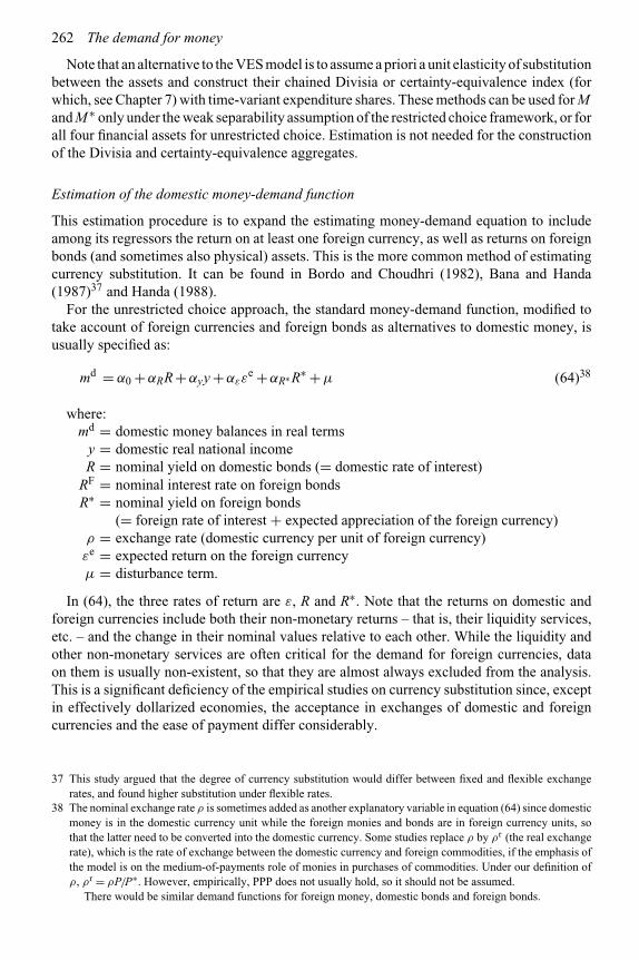
262 The demand for money
Note that an alternative to the VES model is to assume a priori a unit elasticity of substitutionbetween the assets and construct their chained Divisia or certainty-equivalence index (forwhich, see Chapter 7) with time-variant expenditure shares. These methods can be used for Mand M ∗ only under the weak separability assumption of the restricted choice framework, or forall four financial assets for unrestricted choice. Estimation is not needed for the constructionof the Divisia and certainty-equivalence aggregates.
Estimation of the domestic money-demand function
This estimation procedure is to expand the estimating money-demand equation to includeamong its regressors the return on at least one foreign currency, as well as returns on foreignbonds (and sometimes also physical) assets. This is the more common method of estimatingcurrency substitution. It can be found in Bordo and Choudhri (1982), Bana and Handa(1987)37 and Handa (1988).
For the unrestricted choice approach, the standard money-demand function, modified totake account of foreign currencies and foreign bonds as alternatives to domestic money, isusually specified as:
md = α0 +αRR +αyy +αεεe +αR∗R∗ +μ (64)38
where:md = domestic money balances in real terms
y = domestic real national incomeR = nominal yield on domestic bonds (= domestic rate of interest)
RF = nominal interest rate on foreign bondsR∗ = nominal yield on foreign bonds
(= foreign rate of interest + expected appreciation of the foreign currency)ρ = exchange rate (domestic currency per unit of foreign currency)εe = expected return on the foreign currencyμ = disturbance term.
In (64), the three rates of return are ε, R and R∗. Note that the returns on domestic andforeign currencies include both their non-monetary returns – that is, their liquidity services,etc. – and the change in their nominal values relative to each other. While the liquidity andother non-monetary services are often critical for the demand for foreign currencies, dataon them is usually non-existent, so that they are almost always excluded from the analysis.This is a significant deficiency of the empirical studies on currency substitution since, exceptin effectively dollarized economies, the acceptance in exchanges of domestic and foreigncurrencies and the ease of payment differ considerably.
37 This study argued that the degree of currency substitution would differ between fixed and flexible exchangerates, and found higher substitution under flexible rates.
38 The nominal exchange rate ρ is sometimes added as another explanatory variable in equation (64) since domesticmoney is in the domestic currency unit while the foreign monies and bonds are in foreign currency units, sothat the latter need to be converted into the domestic currency. Some studies replace ρ by ρr (the real exchangerate), which is the rate of exchange between the domestic currency and foreign commodities, if the emphasis ofthe model is on the medium-of-payments role of monies in purchases of commodities. Under our definition ofρ, ρr = ρP/P∗. However, empirically, PPP does not usually hold, so it should not be assumed.
There would be similar demand functions for foreign money, domestic bonds and foreign bonds.

The demand function 263
Forced by the lack of data on the non-monetary/liquidity costs of domestic and foreignmonies, the monetary return on foreign currencies is measured by the expected rate ofappreciation of the foreign currency vis-à-vis the domestic currency.39 This expectedappreciation equals (−∂ρ/∂t)e, where ρ is the number of units of the domestic currencyper unit of the foreign one, so that (−∂ρ/∂t)e is the opportunity cost of holding the domesticcurrency rather than the foreign one. Therefore, εe in (64) is measured by (−∂ρ/∂t)e. Inempirical estimations using quarterly data, the proxy usually used for εe is (F −S)/S, whereF is the 90-day forward exchange rate and S is the spot rate. For empirical studies on countriesother than the USA, the foreign currency is usually taken to be the US dollar.
In open economies with perfect financial markets, the domestic and foreign interest ratesare related by the interest rate parity (IRP) condition:
(1 + Rt) = (1 + RFt)(1 + εe
t) (65)
where RF is the rate of interest on foreign bonds and εe(= (∂ρ/∂t)e) is the expected rate ofdepreciation of the domestic currency. The common approximation to (65) is:
Rt = RFt + εe
t (66)
Rt , Rft and εe
t are all arguments of the open-economy money demand function. (66) impliesthat only two of these three variables are independent of each other, so that any two of them,but not all three, should be included in the estimating money demand equation. The twovariables so selected are usually the domestic rate of interest and the expected exchange rateappreciation: many studies set αR∗ = 0 prior to estimation, using the intuition that substitutionbetween domestic money and foreign bonds is likely to be minimal.
(64) is usually estimated in a log-linear form, so that its coefficients represent elasticities.The cross-price elasticity αR is the indicator of price-substitution40 between the domesticcurrency and domestic bonds, and the cross-price elasticity αR∗ is the indicator of price-substitution between the domestic currency and foreign bonds.41 αε is the cross-priceelasticity42 with respect to the return on foreign currencies and can therefore be used asan indicator of CS.
In a four-asset portfolio selection analysis, the signs of any of the three cross-elasticities αε,αR and αρ∗ are not specified by theory and could be negative or positive.43 An empiricallydetermined negative sign is interpreted as evidence of substitution between the domesticcurrency and the relevant asset. While a positive sign is sometimes interpreted as evidenceof complementarity, this interpretation is not necessarily correct since it can reflect some
39 The expected return is the expected rate of depreciation less the cost of holding foreign currencies. This cost canbe very significant where it is illegal to hold and/or deal in foreign currencies, but is minimal in an unregulatedfree financial system.
40 Note that the elasticity of domestic money demand with respect to (∂ρ/∂t)e is a “price” elasticity and as suchdoes not directly measure the elasticity of substitution between the domestic and the foreign currency. Therelationship between the price elasticity and the elasticity of substitution has already been discussed in Chapter 7in connection with Chetty’s procedure.
41 Cuddington (1983) argued that a significant coefficient of the return on foreign bonds is evidence of capitalmovement, not CS, while CS requires the coefficient of ε to possess a negative sign and be significant.
42 The cross-return elasticity is a cross-elasticity with respect to a change in the price (in our context, return) ofanother variable.
43 This sign would be specified only as negative in a two-asset model.

264 The demand for money
other effect. This possibility is especially likely for the sign of αR∗, as we illustrate laterthrough the discussion on the substitution between M and M ∗ in the medium-of-paymentsrole.
Estimation of capital mobility
Capital mobility is distinct from CS and may be defined as the net outflow of funds from thedomestic economy into foreign assets, so that it would be specified by the overall substitutionbetween the sum of the domestic currency and domestic bonds into foreign currency andforeign bonds. This would require the estimation of both the domestic money and bondequations. Therefore, the coefficients in the money demand function alone cannot be used asan indicator of capital mobility.44
8.9.3 The special relation between M and M* in the medium-of-paymentsfunction
Since the domestic currency and foreign bonds are both assets, portfolio selection theoryimplies that an increase in the return on foreign bonds relative to the return on the domesticcurrency (the riskless asset with a zero return) would cause substitution between them, therebyimplying that ∂M/∂R∗ = αR∗ ≤ 0. This effect can be decomposed into two componentsspecified by:
∂M d
∂R∗ =[
∂(M d)
∂R∗
]M∗=M∗
+ ∂M d
∂(M ∗/ρ)
∂(M ∗/ρ)
∂R∗ (67)
In (67), the first term on the right represents direct substitution between M and foreignbonds, holding foreign money balances constant. This (direct) effect occurs because theincrease in foreign bonds increases the opportunity cost of holding domestic money relative toforeign bonds. The second term on the right is an indirect effect occurring through ∂M ∗/∂R∗,which arises because an increase in R∗ also increases the opportunity cost of holding foreignmoney. As these balances decrease, the public has to increase domestic money balances inorder to arrive at the desired level of the overall media of payments needed to finance itsexpenditures.
The direct effect is primarily determined by portfolio selection, which treats domesticmoney as an asset held for its return relative to other assets. Except in conditions wherethe domestic bonds do not exist or their security is doubtful, the significant portfolio switchcaused by a rise in R∗ is likely to be between foreign bonds and domestic bonds (ratherthan domestic money) since both are income-earning assets. It is not likely to be betweenforeign bonds and domestic money. Therefore, while portfolio selection analysis impliesthat (∂M d/∂R∗) |�M∗=0 ≤ 0 , this direct effect is likely to be quite weak in normal financialconditions.
The indirect effect in (67) is the multiple of two elements, ∂M d/∂(M ∗/ρ) and (∂M ∗/ρ)/∂R∗.On the second of these two elements, both the portfolio selection and the transactions demandanalyses imply that (∂M ∗/ρ)/∂R∗ < 0. On the first element, ∂M d/∂(M ∗/ρ) is the substitution
44 This is so even if ε is omitted from the regression. In this case, the coefficient of R∗(= RF + ε) in the estimationof M d is likely to capture both CS and the substitution between domestic currency and foreign bonds.

The demand function 265
between domestic and foreign monies, which constitutes CS. Our earlier discussion onthis point implies that ∂M d/(M ∗/ρ) ≤ 0. Hence, in (67), the second term on the right isnon-negative. Therefore:
[∂M d
∂R∗
]M∗=M∗
≤ 0, (68)
∂M d
∂(M ∗/ρ)≤ 0 and
∂M ∗/ρ∂R∗ ≤ 0 (68′)
so that
∂M d
∂(M ∗/ρ)
∂(M ∗/ρ)
∂R∗ ≥ 0 (68′′)
Since, from (68), the first term (the direct effect) on the right-hand side of (67) is non-positiveand the second one (the indirect effect), from (68′′) is non-negative, the sign of ∂M d/∂R∗in (67) – and hence of αR∗ in (64) – is analytically indeterminate and will depend on therelative magnitudes of the direct and indirect effects. Assuming that the major substitutionin portfolio selection is unlikely to occur between the domestic money and foreign bonds,45
(∂M d/∂R∗) |�M∗=0 in (67) is likely to be relatively small, so that our hypothesis is that thesecond term on the right-hand side of (67) will dominate the sign and magnitude of ∂M d/∂R∗for most economies.
Now focusing on the magnitude of ∂M d/∂(M ∗/ρ), our earlier discussion of this CSeffect implies that it will be relatively weak in economies in which the foreign money isnot extensively used as a medium of payments in domestic transactions.46 However, ineconomies in which foreign monies function as one of the domestic media of payments,∂M d/∂(M ∗/ρ) will be negative and significant. Therefore, in the context of equation (64),if both the domestic and foreign currencies are widely used as media of payments in thedomestic economy and the demand for the overall media of payments is determined bydomestic GDP, an increase in the return on foreign bonds could decrease the holdings ofthe foreign currency in the domestic economy, which need to be balanced by an increase inthe domestic money balances. That is, the increase in R∗ would induce a significant increasein M d, so that the second term in (67) is likely to dominate and αR∗ in (64) should bepositive.
Hence, our hypothesis for partially dollarized economies is that αR∗ should be positiveand significant. By comparison, for economies in which foreign money is not in extensiveusage as one of the media of payments, the first term on the right-hand side of (67) is likelyto dominate, so that αR∗ in (64) should be insignificant or negative.
45 Conversely, the probable substitution is likely to be between domestic and foreign monies, between domesticmoney and domestic bonds, and between foreign money and foreign bonds.
46 For such economies, Handa (1988) specified the domestic currency as the preferred habitat for the domesticmedium of payments, from which substitution into the foreign currency would be relatively low.

266 The demand for money
Estimation of M/(M ∗/ρ)
The third procedure for estimation of the money-demand function focuses on the estimationof M/M ∗ or of M/(M ∗/ρ). We have argued above that there is a special relationship betweenM and M ∗ because of their substitution in domestic payments. This could be captured by aweakly separable preference function over M and M ∗ (as in Bordo and Choudhri, 1982) ora “monetary services production function” (as in Ratti and Jeong, 1994). For such functions,CS can also be assessed by estimating the function for the ratio M/(M ∗/ρ) rather than thedemand function for domestic money only. In the general, unrestricted, case, this ratio willalso be a function of the explanatory variables in (64), so that the corresponding log-linearequation with all variables in logs would be:
M d/(M ∗d/ρ) = f (εe,R,R∗,Y ,ρ) = β0 +βεεe +βRR +βR∗R∗ +βY Y +βρρ (69)
As pointed out earlier, the approximate form of the IRP hypothesis implies that εe, R and R∗are linearly related for an economy with a high degree of capital mobility, so that εe can beleft out of the explanatory variables. β∗
R is likely to be positive for economies in which foreignmoney is significant as a medium of payments in transactions. However, our conjecture isthat βR∗ ≤ 0 for other economies in which the foreign money does not circulate extensivelyin domestic payments because, among other reasons, retailers do not give the bank rate ofexchange and/or charge commissions.
8.9.4 Other studies on CS
In their estimating equation for CS, Ratti and Jeong (1994) claim to combine a “dynamicmonetary services” model with portfolio allocation. Their model47 implies that theoptimal ratio M /(M ∗/ρ), under purchasing power parity and interest rate parity, equals(ρ · P/P∗)(R/RF(1 + ε)), so that, in log-linear term:
M/(M ∗/ρ) = β1(ρ · P/P∗) +β2(R/RF(1 + ε)) (70)
where P∗ is the foreign price level, (ρ · P/P∗) is the real exchange rate, which is includedsince foreign money balances need to be converted to their purchasing power over domesticcommodities, and (R/RF(1+ε)), with R∗ ≡ RF(1+ε), is the relative rate of return on domesticand foreign bonds. Note that if absolute purchasing power parity (PPP) holds, (ρ ·P/P∗) = 1,so that, in (70), M/(M ∗/ρ) = (R/R∗(1+ε)), which implies that, in a regression, β1 should notbe significantly different from zero. If it is, the PPP hypothesis is rejected. But if IRP holds,then (R/R∗(1 + ε)) equals unity, so that M/(M ∗/ρ) = (ρ · P/P∗), implying that β2 shouldnot be significantly different from zero; if it is, the PPP hypothesis is rejected. If both PPPand IRP hold, then M/(M ∗/ρ) = 1, implying that both β1 and β2 should not be significantlydifferent from zero. Further, if neither PPP nor IRP holds, (70) implies that the coefficientsof both (ρ · P/P∗) and (R/R∗(1 + ε)) should be unity. Therefore, (70) seems to represent avery restrictive model, whose value lies not so much in providing estimates of CS but ratherwhether or not either or both PPP and IRP hold.
47 For the details of this model, we refer the reader to Ratti and Jeong (1994). This model does not include moneydirectly in the utility function but relies on a “transactions function” that specifies the real resources needed fortransactions, with “money services” being provided by domestic and foreign money holdings.

The demand function 267
In economies in which domestic residents have limited or no access to foreign bonds,the return on foreign bonds will not enter the domestic money demand function, so thatmulticollinearity between changes in the expected exchange rate and returns on domestic andforeign bonds will not pose a problem. This makes the estimation of CS, and the evaluationof its extent, by the estimated coefficient of the expected exchange rate change more credible.For such a context, De Freitas and Veiga (2006) study CS in the context of six Latin Americaneconomies.48 They use a stochastic dynamic optimizing model in which money reduces thelosses due to frictions in commodity exchanges. They report evidence of CS for Colombia,the Dominican Republic and Venezuela but not for Brazil and Chile, with ambiguous resultsfor Paraguay.
Conclusions
This chapter has examined the form of the money demand function to be used for estimation.One of these uses expected income as its scale variable, while another uses permanent income.Neither is observable, so that a procedure has to be adopted for their estimation. The rationalexpectations hypothesis (REH) was proposed for the estimation of expected income, while theadaptive expectations hypothesis was proposed for the estimation of permanent income. Ofthese, adaptive expectations are backward looking and ignore information that may alreadybe available on the future, but do provide a better measure of permanent income, which isthe average expected level of income for the future rather than expected income for the nextperiod.
This chapter also looked at the use of partial adjustment models (PAMs). These modelsare based on the notion that there are various costs of adjusting money balances quickly,and imply the specific order of the partial adjustment model. The general autoregressivedistributed lag model nests the PAM and the adaptive expectations models. An alternative tosuch a model would be a PAM model with a separate procedure for the rational expectationsestimation of expected income.
The open-economy form of the money demand equation distinguishes between currencysubstitution (i.e. substitution between the domestic and foreign currencies) and capitalmobility, which is mainly substitution between domestic and foreign bonds. There arebasically three procedures for estimation of currency substitution. These are the estimationof a money demand function, a variable elasticity of substitution function and estimation ofthe ratio of domestic to foreign currency holdings.
While portfolio theory seems to imply that there should be considerable and increasingcurrency substitution among the highly open modern economies, the econometric evidenceremains quite mixed. This could be due to the preferred habitat role of domestic moneybalances as the domestic medium of payments. For most economies, foreign monies donot commonly circulate in the economy because of “brokerage costs” imposed by retailerson payments in foreign currencies. However, these costs tend to be trivial for a specificforeign money, which is often the US dollar, in partially dollarized economies, so that sucha money functions as a domestic medium of payments in addition to the domestic money.In this case, there should be a high degree of substitution between domestic money and
48 These authors start with an intertemporal relative risk aversion utility function over consumption in differentperiods and assume that the time spent shopping per unit of consumption expenditures depends on the domesticand foreign monies held.

268 The demand for money
foreign money.49 Note that a fully dollarized economy will not have a distinct domesticmoney.
Summary of critical conclusions
❖ The appropriate scale variable for the demand for money may be current income, expectedincome or permanent income, the last one being a substitute for wealth.
❖ The rational expectations hypothesis is more suitable than adaptive expectations forestimating expected income for the period ahead. For this hypothesis, the unanticipatedcomponent of income is usually estimated as income less the statistical estimate of expectedincome.
❖ The adaptive expectations approach is the more appropriate statistical method for estimatingthe average expected income over the future, i.e. permanent income.
❖ Partial adjustment models provide a way of capturing the lagged adjustment of actual todesired money demand.
❖ In the open economy, currency substitution (CS) also affects the demand for domesticmoney. CS is distinct from capital mobility.
Review and discussion questions
1. Are there significant costs in adjusting actual to desired money balances or in changingbalances between periods? Or are any such costs relatively insignificant but the delayin the adjustment of actual to desired balances occurs as a consequence of the costs ofadjusting commodities and other financial assets to their desired levels? Discuss.
2. Discuss the justification for the use of permanent income in a money demand function.Assuming that adaptive expectations are to be used to derive permanent income, derivethe estimating money demand equation.
Discuss the suitability of rational expectations for estimating permanent income.3. Discuss the justification for the use of expected income in a money demand function.
Assuming that rational expectations are to be used to derive expected income, derive theestimating money demand equation.
Discuss the suitability of adaptive expectations for estimating expected income.4. Starting with a cost function leading to a second order partial adjustment model, and
a money demand function with expected income as the scale variable, derive theappropriate form of the estimating equation for the demand for money.
5. Starting with a cost function leading to a second order partial adjustment model, anda money demand function with permanent income as the scale variable, derive theappropriate form of the estimating equation for the demand for money.
6. Define currency substitution and distinguish it from capital mobility, as well as fromsubstitution between domestic and foreign bonds. How are the returns on foreignmonies and foreign bonds determined? What multicollinearity problems arise in theopen economy money demand equation and how would you choose to resolve them?
49 Ko and Handa (2006) estimate CS in Hong Kong, a partially dollarized economy in which the HK dollar andseveral foreign currencies (US dollar, British pound and the Chinese yuan) circulate in domestic payments, andreport a very significant degree of CS.

The demand function 269
7. Define weak separability. Discuss the role that it plays in specifications of the estimationequations for CS?
8. Present and discuss the three major modes of estimating currency substitution for aneconomy.
References
Arrow, K. “The future and the present in economic life.” Economic Inquiry, 16, 1978, pp. 157–69.Bana, I.M., and Handa, J. “Currency substitution: a multi-currency study for Canada.” International
Economic Journal, 1, 1987, pp. 71–86.Bordo, M.D., and Choudhri, E.U. “Currency substitution and the demand for money: some evidence
for Canada.” Journal of Money, Credit and Banking, 14, 1982, pp. 48–57.Cuddington, J. “Currency substitution, capital mobility and money demand.” Journal of International
Money and Finance, 2, 1983, 111–33.Cuthbertson, K. The Supply and Demand for Money. London: Blackwell, 1985, Ch. 3.De Freitas, M.L., and Veiga, F.J. “Currency substitution, portfolio diversification, and money demand.”
Canadian Journal of Economics, 39, 2006, pp. 719–43.Friedman. M. “The quantity theory of money – a restatement.” In M. Friedman, ed., Studies in the
Quantity Theory of Money. Chicago: Chicago University Press, 1956, pp. 3–21.Giovannani, A., and Turtleboom, B. “Currency substitution.” In Frederick van der Ploeg, ed., The
Handbook of International Macroeconomics. Oxford: Blackwell, 1994.Handa, J. “An empirical study of financial intermediation in Canada.” Journal of Financial and
Quantitative Analysis, 4, 1971, pp. 583–600.Handa, J. “Substitution among currencies: a preferred habitat hypothesis.” International Economic
Journal, 2, 1988, pp 41–62.Kantor, B. “Rational expectations and economic thought.” Journal of Economic Literature, 17, 1979,
pp. 1422–41.Ko, K.W., and Handa, J. “Currency substitution in a currency board context: the evidence for Hong
Kong.” Journal of Chinese Economic and Business Studies, 4, 2006, pp. 39–56.Miles, M.A. “Currency substitution, flexible exchange rates and monetary independence.” American
Economic Review, 68, 1978, pp. 428–36.Mizen, P., and Pentecost, E.J. “Currency substitution in theory and practise.” In P. Mizen,
and E.J. Pentecost, eds, The Macroeconomics of International Currencies. Cheltenham, UK:Edward Elgar, 1996, pp. 8–43.
Muth, J.F. “Rational expectations and the theory of price movements.” Econometrica, 29, 1961,pp. 315–35.
Ratti, R.A., and Jeong, B.W. “Variation in the real exchange rate as a source of currency substitution.”Journal of International Money and Finance, 13, 1994, pp. 537–50.
Sriram, S.S. “Survey of literature on demand for money: theoretical and empirical work with specialreference to error-correction models.” International Monetary Fund Working Paper No. 64, 1999.
9 The demand function for moneyEstimation problems, techniques and findings
This chapter presents the estimating function for money demand, an introduction to theappropriate econometric techniques and a summary of the empirical findings on money demand.On the econometric techniques, a major part of the presentation is on cointegration techniqueswith error-correction modeling for estimating the short-run and the long-run demand formoney.
The empirical evidence clearly confirms the dependence of the demand for money on botha scale variable and an interest rate. The issue of which scale variable should be used – currentincome, permanent income or wealth – is still not settled.
Key concepts introduced in this chapter
♦ Multicollinearity♦ Serial correlation♦ Stationarity♦ Order of integration♦ Unit roots♦ Cointegration♦ Error-correction modeling
The preceding chapters specify the theoretical analyses of money demand and the generalnature of the money demand function. This chapter examines the econometric problems andtechniques associated with its estimation, and presents the findings of some of the relevantempirical studies.
A very large number of empirical studies on the money demand function have beenpublished. It would take up too much space to review even the more important ofthese studies, or to do justice to the ones from which we adopt the results. Amongthe many excellent reviews of these studies in the literature are those by Cuthbertson(1991), Goldfeld (1973), Feige and Pearce (1977), Judd and Scadding (1982), Goldfeldand Sichel (1990), Miyao (1996) and Sriram (1999, 2000). We shall present only thegeneric findings on the more significant issues, especially those on the income and interestrate elasticities and the appropriate measure of the monetary aggregate. We intend to payparticular attention to the findings from studies using cointegration and error-correctionanalysis.

Estimation problems 271
The empirical findings on monetary aggregation reported in Chapter 7 complement thematerial in this chapter. In particular, the empirical findings concerning the Divisia andcertainty equivalence aggregates versus simple-sum aggregates are to be found in Chapter 7rather than this chapter.
Section 9.1 presents a historical review of money demand estimation and its findings.Sections 9.2 to 9.7 discuss some of the econometric problems that can arise with thedata and present the cointegration and error-correction techniques. Section 9.8 presents thefindings of some empirical studies using these procedures. Section 9.9 touches on causality.Section 9.10 provides an illustration of the shifts in income and interest-rate elasticities dueto financial innovations. Section 9.11 focuses on the desperate search for a stable moneydemand function.
9.1 Historical review of the estimation of money demand
By the end of the 1960s, the basic form of the money demand function had evolved as:
md = a0 + aRR + axx (1)
where x is a scale variable. The stochastic form of this function was estimated in either alinear or a log-linear form. During the 1960s, the main disputes were whether money shouldbe defined as M1, M2 or by a still wider definition, whether the interest rate should be short-term or long-term, and whether the scale variable x should be income, permanent income orwealth. The data usually used for estimation was annual.
The 1970s were a period of increasing deregulation of the financial system, with financialinstitutions offering a variety of interest-bearing checking accounts and checkable savingsaccounts. There was increasing use of quarterly data in this decade and of the partialadjustment model discussed in Chapter 8. The latter justified the use of the lagged value ofmoney among the explanatory variables, so that the linear or log-linear form of the commonlyestimated money-demand function was:
mdt = a0 + arrt + ayyt + (1 − γ )mt−1 +μt (2)
where γ was the adjustment parameter and μ was a white-noise disturbance term.In an attempt to eliminate serial correlation, a common problem, in money-demand
functions or to incorporate a partial adjustment model, (2) was often estimated in its firstdifference form. The empirical estimates still indicated the stability of the money demandfunction, but M1 now often, though not always, performed better than M2 and broaderaggregates. The value of the adjustment parameter γ in (2) tended to be roughly between0.20 and 0.5, so that full adjustment to long-run values occurred in about two to six quarters.There was a low impact (one-quarter) real income elasticity (about 0.2) and long-run incomeelasticity less than 1 (often around 0.7), and a low impact interest elasticity (about −0.02 orsmaller) and a long-run interest elasticity roughly between −0.05 and −0.15.1 The empiricalfindings on the income and interest elasticities of money demand in Canada were roughlysimilar.
1 For a summary up to about 1990 of the empirical findings on money demand, see Goldfeld and Sichel (1990).

272 The demand for money
Income and wealth in the money demand function
The period of the 1950s and early 1960s in many countries was one during which theregulatory authority did not allow interest to be paid on demand deposits. Further, the interestrates paid on savings deposits were subject to upper limits, savings deposits could not bedrawn upon by check and a switch from savings deposits to demand deposits often required apersonal visit to the relevant financial institution. Under these conditions, the general findingamong the empirical studies was that M2 did better than either M1 or measures broaderthan M2. The explanatory variables that usually performed best with M2 as the dependentvariable were medium- or long-term interest rates, with wealth or permanent income as thescale variable. The estimating function was normally stable.
For the data covering the 1950s and 1960s in the USA, regression analysis of the demandfor money from equations containing both income and wealth, as well as from equationscontaining only one of these variables, showed that wealth provided a more stable demandfunction for money than current income and that, when both variables were includedsimultaneously, the coefficient of the income variable was insignificant. Permanent incomesimilarly performed better than current income. These results held especially if money wasdefined as M2 or M3 but not as often in studies where the dependent variable was M1. Further,among functions using income, non-human wealth and permanent income, the empiricalestimates showed that functions using a wealth concept gave more accurate predictions ofthe velocity of circulation of money broadly defined – but not as often for M1– than did thosecontaining current income.
The findings on the economies of scale were uneven. Studies using M1 as the dependentvariable often found income elasticities to be less than one, typically around 0.7 or 0.8.Higher income elasticities were usually reported for M2, with some in excess of unity. Thereason for this divergence hinges on the inclusion of interest-earning savings deposits in M2.The demand for savings deposits is likely to reflect more strongly a portfolio demand thandoes M1, so that, with income and wealth positively correlated, the income elasticity of M2will tend to capture to a greater extent the impact of wealth on savings deposits than doesthe income elasticity of M1. This portfolio demand could make them a “superior good” forhouseholds who experience wealth increases during the sample period.
As between the partial adjustment model and adaptive expectations, with US annualdata for 1915–63, Feige (1967) used permanent income as the scale variable and reportedinstantaneous adjustment. However, Goldfeld (1973), with quarterly US data, found less thaninstantaneous adjustment. In general, during the 1970s, studies using quarterly data providedevidence of both adaptive expectations and partial adjustment.
Interest rates in the money-demand function
There are many interest rates in the economy, ranging from the return on savings depositsin banks and near-banks to those on short- and long-term bonds. Near-money assets suchas savings deposits in commercial banks proved to be the closest substitutes for M1, sothat their rate of return seems to be the most appropriate variable as the interest cost ofusing M1.
But if a broader definition of money were used, the interest rate on medium-term or long-term bonds would become more appropriate (the alternative to holding M2 or M3 is longerterm bonds), since the savings components of the broad definition of money themselves earnan interest rate close to the short rate of interest.

Estimation problems 273
The interest rates usually used in estimating money demand are: the interest rate paidon savings deposits in commercial banks, or on those in credit unions (such as MutualSavings Banks and Savings and Loan Associations in the USA, Caisses Populaires in Quebec,Canada); the yield on Treasury bills or on short-term prime commercial paper and the yieldon longer term bonds, such as 3 to 20-year government or commercial bonds. Each of theseinterest rates seems to perform fairly well, sometimes better and sometimes worse than others,in some study or other, and yields different coefficients.
A uniformly good performance, irrespective of which of the interest rates is includedin the regression, is an indication that the various interest rates are related, moving up ordown in a consistent pattern, so that it is immaterial which interest rate is included. Onetheory that points towards such consistency of pattern is the expectations hypothesis on theterm structure of interest rates, i.e. on the yields on assets differing in maturity. Chapter 20presents this hypothesis for the financially well-developed financial markets, pointing outthat it has done remarkably well in explaining the differences in the yields of assets differingin maturity. A consequence of such a relationship among interest rates is that the inclusionof more than one interest rate results in multicollinearity and therefore in biased estimates oftheir coefficients.
However, while the relevant interest rates are closely related, they do not move so closelytogether that any of them will do equally well in estimation, so that usually one or two of themhave to be chosen on empirical grounds for inclusion as regressors. On the wider question ofwhether the demand for money depends on interest rates or not, there is substantial evidencethat the demand for money does depend negatively upon the rate of interest in financiallydeveloped economies. This is also the finding of many studies on the less developed countries(LDCs).
Some studies on the LDCs, however, do not find significant interest rate elasticities fora variety of reasons, including regulatory limits on the interest rates in the economy andinadequate access to banking and other financial facilities. In these cases, very often the rateof inflation rather than the published data on interest rates yields better empirical results.This occurs because the regulated interest rates usually do not accurately reflect the expectedrate of inflation, as market-determined rates do in developed financial markets, so that land,inventories and other real assets, whose prices better reflect the rate of inflation, become moreattractive alternatives than bonds for holding cash.
Various empirical studies have reported that the interest elasticity of money demand isdefinitely negative and significant, and in the range −0.15 to −0.5.
Money demand and the expected rate of inflation
One of the alternatives to holding money is commodities, which have the (expected) rate ofreturn equal to the expected rate of inflation less their storage and depreciation costs. Someof the commodities – as for example, untaxed plots of land – have minimal storage anddepreciation costs, so that the (expected) rate of return on commodities is usually taken tobe proxied by the expected rate of inflation. Therefore, the expected rate of inflation is oneof the arguments in the money-demand function, in addition to interest rates, as Friedman’sanalysis of money demand in Chapter 2 pointed out.
However, in perfect financial markets, for small values of the real interest rate and expectedinflation, the nominal and the real rates of interest are related by the Fisher equation:
Rt = rt +πet (3)

274 The demand for money
where R is the nominal rate of interest, r is the real one and πe is the expected inflationrate. At significant rates of inflation, variations in the real rate tend to be much smaller inmagnitude than the expected inflation rate, so that Rt and πe
t will be closely correlated.Given this close correlation and that between πe
t and the actual rate of inflation πt , R andπ also tend to be closely correlated in periods with significant inflation rates. Therefore,incorporating both Rt and πt in the money demand equations often leads to multicollinearityand biased estimates of their coefficients. As a way around these statistical problems, πt
is often dropped in favor of Rt from the estimated money demand equations for developedeconomies with market determination of Rt . However, economic theory implies its inclusionin addition to the inclusion of interest rates, so that its omission could result in a misspecifiedequation.
In economies such as the LDCs’, where the financial markets are not well developed,ceilings are often imposed on the rates of interest that can be legally paid and therecould exist both an official interest rate and a free or black market rate. Further, reliabledata on interest rates may not be available. In these cases, πe
t should be retained in theestimating equation in addition to – and sometimes even to the exclusion of – the interestrate. Note that the proper variable is πe
t and that πt is only one of the possible proxiesto it.2
The liquidity trap
One of the questions of interest in monetary theory since the time of Keynes, discussed inChapter 2 above, has been about the empirical existence of the liquidity trap. Keynes positedthe possible existence of such a trap, though he also expressed the belief that he did not knowof any case where it had existed.
One possible method of testing for the existence of the liquidity trap is to estimate thedemand for money separately for periods with differing ranges of the prevailing interestrates. Estimates showing that the interest elasticity of demand tends to increase in periodswith lower ranges of interest rates, and especially those showing a substantial increase atvery low interest rates, can be interpreted as raising a presumption that the liquidity trapcould have existed empirically. However, empirical studies so far have not revealed sucha pattern. Velocity functions estimated separately for each decade did not find any higherinterest elasticity of the demand for money during the 1930s, when interest rates were lowthan during other decades with higher interest rates. Further, regressions incorporating datafrom the 1930s did fairly well in predicting velocity during the subsequent decades, implyingthat the interest elasticities during the 1930s did not differ substantially from those of morenormal conditions. These studies indicate that the liquidity trap does not seem to have existedin the US economy for any significant period, if at all, during the Great Depression of the1930s and is even less likely a possibility for other periods.
Theoretically, the liquidity trap should come into existence if the nominal yield on bondsbecomes zero. The Japanese economy in recent decades provides an interesting experiment onthe liquidity trap since it has had short-term interest rates close to zero. Bae et al. (2006) havestudied different money demand functions for Japan using linear and non-linear cointegrationtechniques with quarterly data from 1976:1 to 2003:4. They report that the interest elasticityfor their various monetary aggregates, including M1, is much higher at low interest rates than
2 If the real rate of interest were constant, the nominal rate of interest would become the better proxy for π et .

Estimation problems 275
at higher rates, thereby favoring the conjecture that the liquidity trap may exist at interestrates that are zero or close to zero.
Shifts in the money demand function
Much greater impact of financial deregulation was felt in the 1980s than had been permittedor achieved in the 1970s. Further, technological and product innovation in the financial sectorwas very rapid. Computers also came into general use in firms and households, and permittedmore efficient management of funds. By the end of the 1980s, automatic tellers for electronictransfer and withdrawal of funds from both demand and savings accounts had becomecommon, and were more numerous than bank branches. Many new variants of demand andsavings deposits had been created and the distinction between demand and savings deposits interms of their liquidity became blurred almost to the point of disappearance, though savingsdeposits still paid higher interest but also imposed higher charges. Deregulation, innovationand technological change resulted in a failure of the quarterly specification for money demand,whether money was defined narrowly or broadly.
These developments in the 1980s led to the estimated demand functions performingpoorly, with unstable money demand and with a highly variable velocity of circulation.The econometric tests also became much more sophisticated than in earlier periods. Amongthese, econometric tests of the money and income time series showed that they were notstationary. To deal with this, cointegration analysis became one of the preferred techniquesand showed that money and income were indeed cointegrated, as were interest rates withthem over many periods.
9.2 Common problems in estimation: an introduction
This section is intended to show that the estimation of the money-demand function isnot a simple and straightforward matter, and that application of the classical least-squaresregression technique to its estimation need not provide reliable estimates. The section providesa brief treatment of the common problems encountered in money demand estimation and isnot meant to provide a complete, in-depth or rigorous treatment of the econometric problemsdiscussed or of the appropriate econometric techniques. These are left to econometricstextbooks such as Davidson and Mackinnon (1993).
The general form of the demand function for real balances implied by the transactions,speculative, buffer stock and precautionary analyses is of the type:
M d/P = md = m(R1, . . .,Rm,πe,y,w) (4)
where:M = nominal balancesm = real-money balancesP = price level
πe = expected rate of inflationRi = rate of return on ith near-money asset, i = 1, . . ., my = real income/expendituresw = real wealth.
The following subsections consider some of the econometric issues that arise in theestimation of such a money demand function.

276 The demand for money
9.2.1 Single equation versus simultaneous equations estimation
From a general equilibrium viewpoint, the rate of return on each of the near-money assetsis influenced by the demand and supply of money and also by the demands and supplies ofrisky assets. A general empirical study of the demand for money would then simultaneouslyestimate the demand and supply functions for all the financial assets, where the demandfunction for the ith asset is:
xi = xi(R1, . . ., Rm,Rm+1, . . ., Rn,πe,y,w) (5)
The definitions of the symbols are:
xi = real quantity of the ith monetary asset, i = 1, . . ., mRj = rate of return on the jth non-monetary asset, j = m + 1, . . ., n.
Note that from a rigorous general equilibrium viewpoint, each asset should be homoge-neous. A general equilibrium study becomes an extremely large enterprise and poses its owneconometric problems. Most studies of the demand for money have been partial and, forstatistical and other reasons, have used various degrees of aggregation in defining money.They also often confine the explanatory variables to one rate of interest and either income orexpenditures or wealth. However, whether or not one is estimating the demand functions forseveral assets simultaneously, it is important to consider the cross-equation restrictions thatthe relevant theory might imply for them. We illustrate these in the following for the case ofthe allocation of a portfolio between money and bonds, as analyzed in Chapter 5.
9.2.2 Estimation restrictions on the portfolio demand functionsfor money and bonds
Chapter 5 implied that the general form of the speculative demand functions for assets is:
xdi = xd
i(μ,σ ,ρ,W ) i = 1, . . ., n − 1 (6)
where μ, σ , and ρ are respectively the vectors of the mean returns, the standard deviationsand the correlation coefficients among the values of the assets, and W is the wealth allocatedamong the assets. (6) and the portfolio budget constraint imply that:
xn = W −�i xdi(μ,σ ,ρ,W ) i = 1, . . ., n − 1 (7)
so that the demand function for one of the assets must be derived as a residual from theestimated demand function of the other assets. Alternatively, if the demand functions for allthe assets are being estimated, the appropriate cross-equation restriction must be imposedon the estimating equations. As an illustration of this, the restrictions imposed by (7) for thetwo-asset case of money (M ) and the composite bond (B) are set out below.
Suppose the estimating equations for M and B are linear and are specified as:
M = a0 + a1Rm + a2Rb + a3W (8)
B = b0 + b1Rm + b2Rb + b3W (9)

Estimation problems 277
where Rm is the nominal return on money and Rb is the nominal return on bonds. The budgetconstraint on M and B is:
M + B = W (10)
Substituting (8) and (9) into (10) yields:
(a0 + b0) + (a1 + b1)Rm + (a2 + b2)Rb + (a3 + b3 − 1)W = 0 (11)
To satisfy (11) for all possible values of the variables, each term in it has to be zero. Therefore,we must have:
a3 + b3 = 1 (12)
ai + bi = 0 i = 0,1,2 (13)
Failure to impose these restrictions on the estimated coefficients in the simultaneousestimation of both demand functions will generally yield estimated values of the coefficientsthat are not consistent with the budget constraint and are therefore not valid. In cases where asingle demand function, say for money, is estimated, and its estimated coefficients seemto be quite plausible, the implied values of the coefficients for the bond equation maynot prove to be accurate or even plausible. For example, if the estimated elasticity of thedemand for money is much larger than one, this would in turn imply that the elasticityof the demand for all other financial assets is correspondingly less than one, which maynot be plausible for the economy and the period in question, thereby leading to a rejectionof the estimated money demand function. Therefore, if it is feasible, it would be better toestimate simultaneously the complete system of demand equations and impose appropriaterestrictions on the coefficients. However, this is not always feasible and often exceeds theresearcher’s interests, so that most studies tend to confine themselves to the estimation ofonly the money-demand function.
9.2.3 The potential volatility of the money demand function
Note that the coefficients ai, i = 0,1,2,3 in the money-demand function (8) depend uponthe means, the standard deviations and the correlation coefficients of the expected terminalvalues of the assets, for all of which the subjectively – not objectively – expected future(not the past actual) values are the relevant ones. If these characteristics of assets change,the implied coefficients will change and the demand functions will shift. In the real world,subjective expectations on the returns and future values of the financial assets continuouslyshift for a variety of reasons, so that the subjectively based characteristics of assets areconstantly changing. These sources of shifts can be classified into (i) shifts in subjectiveprobability estimates because of changing market conditions, (ii) shifts in policies whichshift the outcomes and their probability functions, and (iii) innovations in the paymentsmechanism, such as the introduction of ATMs and electronic banking.
Keynes (1936, Ch. 13) focused on (i) and argued that the expectations of asset returns,and hence of these characteristics, are very volatile. This argument implies that the demandfunctions for money and other financial assets would be constantly shifting, so that they couldnot be properly estimated or, if estimated, would be worthless – unless the nature of the shiftcould be specified and adjustments made for it – as guides for future policies.

278 The demand for money
The Lucas critique (in Chapter 17) of estimated functions used for policy purposes focuseson (ii) above and argues that, if a change in policy – for example, in the monetary regime,tax laws, banking and financial regulations, relevant political stance, etc. – shifted thecharacteristics of the returns to the assets, the demand functions would shift and the priorestimated forms would no longer be valid. Hence, specific forms of the demand functionswill not hold across policy regimes.
The above arguments caution that, since the money demand and supply functions, aswell as other relevant policy functions, are constantly changing and definitely do so overdecades, the validity of using data over long periods of time to estimate a demand functionwith constant coefficients should be extremely suspect. This is especially so in a period offinancial innovation, which keeps changing the relative characteristics of the existing assetsand, over time, keeps adding newer ones to the marketplace.
9.2.4 Multicollinearity
Another statistical problem encountered in partial studies is the multicollinearity problem.Suppose that the demand for money is related to both income and wealth but that incomeand wealth are themselves highly correlated. The estimate of the relationship between moneybalances demanded and income is then influenced by the relationship between income andwealth and vice versa, so that the estimated relationship may not be an accurate measure ofits actual value.
Similarly, the various rates of return are highly correlated, so that the estimates of thecoefficients of the rates of return in the money demand function in the economy also tend tobe biased and must be treated with caution.
If there is fairly close correlation among a set of variables, one solution to themulticollinearity problem is to use only one of the variables in the set and interpret itsestimated coefficient as representing the collective effect of all the variables in the set.For instance, given the close correlation among the interest rates, most money demandfunctions include among the independent variables only one interest rate in order toavoid multicollinearity. This is usually a short-term rate, such as the Treasury bill rate.However, some studies include both a short-term and a long-term interest rate. As betweencurrent income and permanent income or wealth, while some studies include only currentincome, others include permanent income, with multicollinearity between these two variablespreventing the simultaneous inclusion of both.
9.2.5 Serial correlation and cointegration
Most regression techniques assume that the error terms are serially uncorrelated and havea constant variance. These should be checked for the estimated error. If it does not satisfythese conditions, as often proves not to be so, the estimated coefficients will be biased and theappropriate techniques that can ensure unbiased estimates have to be used. The techniquesoften used for correcting for serial correlation include estimating the money demand functionin a first-difference form and using a technique with a built-in correction for the relevant orderof serial correlation.
Regression analysis used for deriving the money-demand function assumes that thevariables are stationary. A variable is not stationary if it has a trend or/and serial correlation.Many of the variables in the money demand function, such as income and the money stock,are not stationary. If this happens, the use of classical regression techniques, such as one-stage

Estimation problems 279
least squares, two-stage least squares, etc., yield biased estimates of the coefficients of theindependent variables. The preferred procedure in such cases is that of cointegration analysis.
9.3 The relationship between economic theory and cointegrationanalysis: a primer
This section presents a brief introduction to stationarity and cointegration analyses. Thereader is referred to econometric textbooks for a proper treatment of these topics.
9.3.1 Economic theory: equilibrium and the adjustment to equilibrium
An economic theory is intended to explain the determination of the actual values of a selectedeconomic variable or of several economic variables. As the starting point for the followingexposition, we focus on the determination of a single economic variable, say y. The theoryon its determination examines three questions:
1 Does an equilibrium relationship exist between the dependent variable y and itsexplanatory variables x (= x1,x2, . . .)? Suppose that such a relationship exists and isof the form:
yt = α0x0 +α1x1 +α2x2 +·· ·+αnxn (14)
where x0 is taken to be constant, and y and x could be the levels of the variables, theirfirst differences or rates of change, etc., or some mix of these, and the relationship couldbe linear or non-linear. For the following exposition, the equilibrium relationship isassumed to be among the levels (or the log values) of the variables and to be a linear one.The estimation equation, expanded to include lagged values of the dependent variabley and the explanatory variables x on the right-hand side, becomes an autoregressivedistributed lag (ARDL) equation, whose treatment is presented in the Appendix to thischapter.
If all the variables in the relationship are stationary, classical least-squares techniquescan yield unbiased estimates of the coefficients of the variables. However, if some of thevariables in the relationship are not stationary, these techniques do not yield unbiasedestimates. The cointegration estimation technique is likely to yield better results. Todetermine the technique that is appropriate, the stationarity or otherwise of each of thevariables has first to be determined by stationarity tests. These are discussed later.
2 Is the equilibrium unique? It is assumed that there is a unique equilibrium for the givenstructural specification of the equations of the model.
3 Is the equilibrium relationship between y and x stable or unstable? Assuming it to bestable, there would be a dynamic adjustment path during the disequilibrium following adisturbance to the equilibrium relationship. The dynamic path can be of different types,requiring different specifications of the adjustment process.3 It is often not clear whichone is the empirically relevant process for the structure in question. The most commonassumption is that the adjustment process is linear (or log-linear). The estimation of the
3 Among these are the partial adjustment models, the error-learning model, etc., presented in Chapter 8.
280 The demand for money
adjustment process and its implications for the stability of equilibrium are discussed laterunder the heading of error-correction models (ECMs).
9.4 Stationarity of variables: an introduction
The equilibrium relationship between the endogenous variable y and the vector x ofexplanatory variables was specified above as:
yt = α0x0 +α1x1 +α2x2 +·· ·+αnxn (15)
Estimation of this equilibrium relationship by classical regression techniques requires thateach of the variables be stationary.
A variable zi is said to be stationary if its mean, variance and covariances with the othervariables in the relationship are finite and constant. The usual symbols for these are:
E(zi) = μi
V (zi) = σii = σ 2i
COV(zi,zj) = σij
The stationarity of zi implies that these moments of its distribution will remain unchanged,except for random differences, over different sample periods. Conversely, if estimationover different sample periods yields different estimated values of these moments, thevariable is likely to be non-stationary. If any of the variables in the relationship impliedby the theory is non-stationary, then the estimates obtained by classical least-squaresregressions of the equilibrium relationship among the variables will differ among thevarious sample periods, so that the estimated relationships will not accurately reveal the truerelationship.
Causes of non-stationarity
The potential causes of non-stationarity are:
1 The mean value of the variable is not stationary, due to a trend.2 The variance of the variable and its covariances with other variables are not stationary.
This is due to serial correlation.
If the variables in the estimation are not stationary due to serial correlation, twodifferent types of estimation procedures can be attempted for estimating the true equilibriumrelationship. One of these is to render the data series stationary prior to estimation, such asby employing a procedure for eliminating serial correlation. To render a series (with serialcorrelation) stationary, each would be differenced once or more times until its derived seriesis stationary. Alternatively, a correction for serial correlation, such as the Cochrane–Orcuttmethod, can be used in the estimation process. Classical regression techniques, such as one-stage or two-stage least squares, often employ such procedures to deal with non-stationarytime series.
An alternative to the above procedure is to use the following property of the equilibriumrelationship, with y as the dependent variable and, for illustration, only x1 and x2 as the

Estimation problems 281
explanatory ones. Assume, as before, that the equilibrium relationship is linear in the levels(or log values) of the variables, so that it is of the form:
yt = α0 +α1x1 +α2x2 (16)
which can be rewritten as:
yt −α0 −α1x1 −α2x2 = 0 (17)
In this equation, since the right-hand side (which is zero) is stationary, the compositevariable (yt −α0 −α1x1 −α2x2) on the left-hand side must also be stationary. Hence, whilethe individual variables are not stationary, their linear combination given by (17) would bestationary. The appropriate linear combination is one with the coefficients (1−α0 −α1 −α2).Note that α0 is the (coefficient of the) constant term. The vector (1−α0 −α1 −α2) is called thecointegrating vector (in this case, with the coefficient of the dependent variable normalized tounity) and (17) is called the cointegrating equation. Empirical analysis requires an appropriateestimation procedure that will provide unbiased estimates of this vector. A few points aboutthe above relationship need to be noted.
• Multiplying each of the coefficients by a constant yields a stationary variable, so thatany multiple of the cointegrating vector is also a cointegrating vector.
• It is quite appropriate to set the coefficient of the endogenous variable as unity, so thatit is customary to normalize the cointegrating vector in this way.
• The signs of the coefficients of the explanatory variables in the cointegrating vector andequation are the reverse of those in the equilibrium relationship.
• If the equilibrium relationship is linear in the logs of the variables, then the cointegratingvector will specify (with signs reversed) the elasticities of the endogenous variable withrespect to the explanatory variables.
The next section discusses the sources of non-stationarity of the variables and the estimationprocedures for determining whether a variable is stationary or not.
A non-stationary mean due to a trend
A trend in a variable will make its mean non-stationary. An example of this occurs if:
zt = α0 +α1t +μt (18)
where z is the variable in question, t is time and μ is white noise.4 In this case, data samplesover different periods will yield different mean values of z, since:
Ezt = α0 +α1Et
A variable that is nonstationary because of the presence of a trend can be transformed byremoving the trend into a corresponding variable (i.e. zt − α1t) that is stationary. Such avariable is said to be trend-stationary (TS).
4 That is, μ is a stationary disturbance term, with a zero mean and finite and constant variance and covariances.
282 The demand for money
Non-stationary variances and covariances because of serial correlation
This type of non-stationarity arises if the variable behaves according to:
zt = α0 + zt−1 +μt (19)5
where μt is white noise. zt is said to follow a random walk if the constant term α0 is zero;it follows a random walk with drift if α0 is not zero. The value of zt depends on the actualvalue of zt−1 (which includes the actual value of μt−1), so that there is a stochastic tendencyfor the mean of the variable to change over different data samples.
Rewrite this equation as:
�zt = zt − zt−1 = α0 +μt (20)
where �zt(= zt − zt−1) is stationary. Therefore, a variable that is non-stationary becauseit follows a random walk can be rendered stationary by taking its first difference. Such avariable is called difference-stationary (DS). If taking the first difference of a series makes itstationary, it is said to be integrated of order 1, which is written as I(1).
Note that if a series is I(1), taking its first difference will yield a stationary series. But ifthe series also has a time trend, the first difference of the series will still possess a trend, sothat it will not be trend-stationary. An adjustment for this trend will have to be made in theestimation procedure.
Non-stationarity because of a shift in the value of the variable
Note that a variable may be stationary but that its data sample may indicate non-stationaritybecause of a shift at some point in its time series. In this case, classical least-squares can stillbe used with the shift captured through the use of a dummy variable.
9.4.1 Order of integration
In the general case of serial correlation, a variable may follow the process:
zt = α0 + zt−p +μt (21)
In this case, the variable would have to be differenced p times to arrive at a stationary series.The variable is then said to be integrated of order p and is designated as I(p).
In the case of difference-stationary data, while using the appropriate number of differencesof the variables does eliminate the problems posed by the non-stationarity of the levelsof the variable, a regression using differenced data eliminates the relationship among thelevels of the variables, so that the regression will not provide estimates of the long-runrelationship between the levels of the dependent and the independent variables in theestimating equation. Therefore, the use of differenced data is not a proper strategy for findingthe equilibrium relationship among the levels of the variables. For example, in the context
5 This equation implies serial correlation of the error over time since substitution in it of the equation for the laggedterm implies that zt = 2α0 + zt−2 +μt +μt−1, so that the error (μt +μt−1) in period t will be correlated with theerror μt−1 in period t−1. Repeated substitutions of the equation for the lagged term will, in fact, yield an equationwhose error term is correlated with the errors in all previous periods.
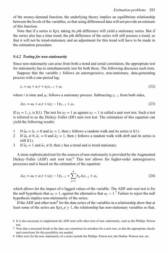
Estimation problems 283
of the money-demand function, the underlying theory implies an equilibrium relationshipbetween the levels of the variables, so that using differenced data will not provide an estimateof this function.
Note that if a series is I(p), taking its pth difference will yield a stationary series. But ifthe series also has a time trend, the pth difference of the series will still possess a trend, sothat it will not be trend-stationary and an adjustment for this trend will have to be made inthe estimation procedure.
9.4.2 Testing for non-stationarity
Since non-stationarity can arise from both a trend and serial correlation, the appropriate testfor stationarity has to simultaneously test for both these. The following discusses such tests.
Suppose that the variable z follows an autoregressive, non-stationary, data-generatingprocess with a one-period lag:
zt = a0 + a1t + a2zt−1 +μt (22)
where t is time and μt follows a stationary process. Subtracting zt−1 from both sides,
�zt = a0 + a1t + (a2 − 1)zt−1 +μt (23)
If a2 = 1, zt is I(1). The test for a2 = 1 as against a2 < 1 is called a unit root test. Such a testis referred to as the Dickey–Fuller (DF) unit root test. The estimation of this equation canyield the following results:
1 If a0 = a1 = 0 and a2 = 1, then z follows a random walk and its series is I(1).2 If a0 = 0, a1 = 0 and a2 = 1, then z follows a random walk with drift and its series is
still I(1).3 If a2 = 1 and a1 = 0, then z has a trend and is trend-stationary.
A more sophisticated test for the sources of non-stationarity is provided by the AugmentedDickey–Fuller (ADF) unit root test.6 This test allows for higher-order autoregressiveprocesses and is based on the estimation of the equation:
�zt = a0 + a1t + (a2 − 1)zt−1 +n∑
j=1
bij�zt−j +μt (24)
which allows for the impact of n lagged values of the variable. The ADF unit root test is forthe null hypothesis that a2 = 1, against the alternative that a2 < 1.7 Failure to reject the nullhypothesis implies non-stationarity of the series.
If the ADF and other tests8 for the data series of the variables in a relationship show that atleast some of the series are I(p), p ≥ 1, the relationship has non-stationary variables so that,
6 It is also necessary to supplement the ADF tests with other tests of non–stationarity, such as the Phillips–Perrontest.
7 Note that a structural break in the data can sometimes be mistaken for a unit root, so that the appropriate checksand corrections for this possibility are needed.
8 Other tests for the non–stationarity of a series include the Phillips–Perron test, the Durbin–Watson test, etc.
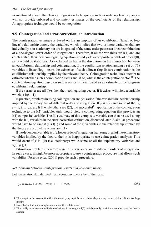
284 The demand for money
as mentioned above, the classical regression techniques – such as ordinary least squares –will not provide unbiased and consistent estimates of the coefficients of the relationship.An appropriate technique would be cointegration.
9.5 Cointegration and error correction: an introduction
The cointegration technique is based on the assumption of an equilibrium (linear or log-linear) relationship among the variables, which implies that two or more variables that areindividually non-stationary but are integrated of the same order possess a linear combinationof a one-degree lower order of integration.9 Therefore, if all the variables are I(1) and arecointegrated, then their cointegrating equation would yield a composite variable of order I(0),i.e. it would be stationary. As explained earlier in the discussion on the connection betweenan equilibrium relationship and cointegration, if the equilibrium relation among a set of I(1)variables is linear (log-linear), the existence of such a linear (log-linear) combination is theequilibrium relationship implied by the relevant theory. Cointegration techniques attempt toestimate whether such a combination exists and, if so, what is the cointegration vector.10 Thecointegration equation based on such a vector is then treated as an estimate of the long-runequilibrium relationship.
If the variables are all I(p), then their cointegrating vector, if it exists, will yield a variablewhich is I(p − 1).
In practice, problems in using cointegration analysis arise if the variables in the relationshipimplied by the theory are of different orders of integration. If y is I(2) and some of the xi,i = 1,2, . . . ,n, are I(1) while others are I(2), the successful11 application of the cointegrationtechnique to the I(2) variables only would yield a cointegrating equation that provides anI(1) composite variable. The I(1) estimate of this composite variable can then be used alongwith the I(1) variables in the error-correction estimation, discussed later. A similar procedurewould have to be used if y is I(1) and some of the xi variables in the relationship implied bythe theory are I(0) while others are I(1).
If the dependent variable is of a lower order of integration than some or all of the explanatoryvariables implied by the theory, then it is inappropriate to use cointegration analysis. Thiswould occur if y is I(0) (i.e. stationary) while some or all the explanatory variables areI(p), p ≥1.
Estimation problems therefore arise if the variables are of different orders of integration.In such a case, it might be more appropriate to use a cointegration procedure that allows suchvariability. Pesaran et al. (2001) provide such a procedure.
Relationship between cointegration results and economic theory
Let the relationship derived from economic theory be of the form:
yt = α0x0 +α1x1 +α2x2 +·· ·+αnxn (25)
9 This requires the assumption that the underlying equilibrium relationship among the variables is linear (or log-linear).
10 Note that not all data samples may show this relationship.11 This really requires an equilibrium relationship among the I(2) variables only, which may not be what the theory
asserts.

Estimation problems 285
If the variables y,x1, . . .,xn are all I(1), the general form of the cointegrating vector, if one isfound, is:
f (y,x1, . . .,xn) = 0
This relationship is log-linear or linear depending upon whether the data was in logs or not.The form of the cointegrating equation is:
yt −α0x0 −α1x1 −α2x2 −·· ·−αnxn = 0 (26)
where x0 represents the constant term. As mentioned earlier, its signs of the coefficients ofthe explanatory variables have to be reversed to arrive at the original equation (25).
Because of potential econometric problems, various econometric checks (discussed later)are applied to check the econometric acceptability of the estimated coefficients. However,even if the estimate is acceptable on the basis of the econometric tests, the estimatedcointegrating vector may still not be a plausible estimate of the true equilibrium economicrelationship. From the perspective of economic theory, this plausibility is judged by checkingwhether the signs of the cointegrating vector are consistent with those implied by the theoryand whether the estimated magnitudes of the normalized cointegrating equation are plausiblein terms of the theory, intuition and estimates obtained by other studies. If this is not so, theestimated cointegrating vector will have to be rejected as an estimate of the true equilibriumrelationship.
Deviations from the equilibrium relationship: the error-correction assumptionfor adjustments in disequilibrium
It was assumed earlier that the equilibrium relationship between the endogenous variableand the vector of explanatory variables is stable and unique. Cointegration literature labelsthis equilibrium relationship – and its estimate by the cointegrating vector – the long-runrelationship.
Since the equilibrium has been assumed to be stable, any deviations from it will becorrected through an adjustment process.12 In cointegration analysis, this adjustment processis often referred to as the dynamic adjustment or as the short-run relationship betweenthe endogenous variable and the explanatory variables. Cointegration techniques assumethat the dynamic adjustment follows a linear or log-linear error-correction process, ratherthan some other one. This process is in the nature of a partial linear adjustment eachperiod.13
The cointegration literature refers to its adjustment estimation technique as “the error-correction model” (ECM). This model specifies the change in the endogenous variable y
12 Engle and Granger (1987) present a theorem showing that cointegration among a set of variables impliesshort-run dynamics that return the variables to the long-run cointegrating relationship. This follows fromthe assumption of the stability of equilibrium and that the cointegrating vector captures the equilibriumrelationship.
13 This error-correction element is somewhat similar to the linear first-order partial adjustment process, as wellas to the error-learning process, both explained in Chapter 8. For comparison, the first-order PAM for theadjustment in y would be yt − yt−1 = γ (y∗
t − yt−1), 0 ≥ γ ≥ 1, where y∗t would be the long-run or desired
value of yt .

286 The demand for money
as a function of last period’s error between the actual and the equilibrium value ofthe dependent variable and of the change in each of the explanatory variables of theequilibrium relationship. Other variables, provided that they are stationary, can also beintroduced in the ECM. The linear specification of the error-correction element of the ECMis specified as:
�yt = θ (yt−1 − y∗t−1) +·· · (27)
where �yt = yt − yt−1,y∗ is the equilibrium value (calculated from the estimated coin-tegrating vector), and y changes each period by the fraction θ of the previous period’sdeviation of the actual value from the equilibrium value y*. For the equilibrium to bestable (equilibrium-reverting), we need θ ≤ 1. The complete ECM equation would havethe form:
�yt = a0 −p∑
i=2
ai�yt−i+n∑
j=1
q∑i=1
bj,t−i�xj,t−i − θECMt−1 +ηt (28)
where the lag lengths p and q have been optimally determined and:
ECMt−1 = yt−1 − α0 −n∑
j=1
αjxjt−1 (29)
9.5.1 Cointegration techniques
The two popular cointegration procedures for determining the equilibrium relationship orrelationships among non-stationary variables are the Engle–Granger (Engle and Granger,1987) and the Johansen – also called the Juselius-Johansen – procedures (Johansen andJuselius, 1990; Johansen, 1988, 1991). The most common application of these procedures iswhen all the variables are I(1).
Engle–Granger method for a reduced-form equation14
For the estimation of the cointegration vector and its associated error-correction dynamicadjustment equation, the Engle–Granger method uses a two-stage procedure. In thefirst stage, it estimates the cointegrating vector among the I(1) variables for a givenequilibrium relationship and tests the residuals for stationarity. If these residuals arestationary, as they should be if all the variables are I(1), the second stage uses them toestimate the dynamic short-run response of the dependent variable by the error-correctionmodel.
The Engle–Granger technique is quite appropriate if all the explanatory variables areexogenous. Often, a model has several endogenous variables, so that it possesses severalequilibrium relationships among its variables. In this case, the Johansen procedure would bepreferable to the Engle–Granger one.
14 A reduced-form equation has only one endogenous variable, whose explanatory variables are all exogenous.

Estimation problems 287
Johansen cointegration procedure for a model with several endogenousvariables15
In a model where more than one variable is endogenous, there would be more than oneequilibrium relationship among the variables. The Johansen cointegration procedure is thenthe preferable one since it treats all the variables in the estimation process as endogenous andtries to simultaneously determine the equilibrium relationships among them. In addition, thisprocedure provides estimates of the cointegrating vectors and the error-correction model inone step. These advantages have made the Johansen procedure the more common one in thecointegration literature.
Assuming that all the variables being considered are I(1), the Johansen procedure (a) takesall the I(1) variables to be as if endogenous and related by a vector-autoregressive (VAR)structural model, (b) uses the maximum likelihood estimation for the VAR model, and(c) derives a set of cointegrating vectors. The number of cointegrating vectors is determinedby the eigenvalue and trace tests. The maximum number of independent equilibriumrelationships that can exist among a set of endogenous variables has to be one less than thenumber of variables.16 Therefore, the maximum number of significant cointegrating vectorsshould be one less than the number of variables in the VAR model.
The propensity of the Johansen procedure to yield several (significant) cointegratingvectors among the variables is an asset but also raises two troublesome issues:
1 Which vector should be treated as the estimate of which one of the equilibriumrelationships among the variables? That is, a choice has to be made among theavailable cointegration vectors for the particular economic relationship being sought.This choice is usually made on the basis of the signs implied by the theory for thecoefficients and the estimated magnitudes of the coefficients falling within a plausiblerange.
2 Any linear combination of the estimated cointegrating vectors is also an admissiblecointegrating vector. Therefore, one can generate an infinite number of combinations,many of which are usually likely to fit the requirements of the appropriate signs andmagnitudes being sought for a specific relationship. The linear combinations can besearched for this purpose. However, this search can easily degenerate into “vector-mining.”
To illustrate, in some applications of the Johansen technique to money-demand estimation,it is found that the elements of none of the cointegration vectors possess signs consistent withthe a priori expectations on the elasticities of the money demand function. Alternatively,these elements could be such as to imply implausible magnitudes of the elasticities. Theseproblems could arise from the limited sample size, inaccuracies in the data, misspecificationin the set of variables, breaks in the data, etc. But it is also possible to argue that, since a linearcombination of the cointegrating vectors is also a cointegrating vector, one could try to findthat linear combination of the cointegrating vectors such that the elements have the desiredsigns and magnitudes in a plausible range. However, this amounts to “mining the vectors,”so that the results often fail to convince other researchers.
15 Such a model would be a structural one.16 Given the assumption of linearity (log-linearity) of the equilibrium relationships among n variables, there can
be at most (n−1) independent relationships among them.

288 The demand for money
To conclude, while the Johansen technique provides econometric evidence on the existenceof long-run relationships among a set of variables, the identification or derivation of thestructural coefficients of the model from the elements of the cointegration vectors can bequite problematical.
9.6 Cointegration, ECM and macroeconomic theory
Economic theory often implies more than one long-run relationship among any given setof economic variables. For example, in the IS–LM model, money demand depends uponnational income and interest rates, while national income – as do interest rates – dependson the money supply, which equals money demand in equilibrium. Assuming these threevariables to be all I(1), such a simultaneous determination of economic variables implies thepossible existence of a maximum of two cointegrating vectors among them. In general, forn variables, there could be (n − 1) independent cointegrating vectors. This poses a problemsince the cointegration technique does not identify a given cointegrating vector with a specificeconomic relationship. For instance, suppose two cointegrating vectors are found amongmoney, income and interest rates. The econometric estimation by itself does not make itclear which one of the cointegrating vectors specifies the money demand relationship. Thishas to be decided by the researcher on the basis of the signs imposed by economic theoryon the coefficients of the money demand relationship and on the basis of the plausibilityof the magnitudes of the elements in the cointegrating vectors. The elements of the selectedcointegrating vector are then taken to specify the respective long-run coefficients of the linear(or log-linear) money demand function.
Now, assuming that a cointegrating vector exists, the ECM can be used to capturethe adjustment of the dependent variable to the long-run equilibrium specified by thecointegrating vector. Among the characteristics of the ECM are:
1 It defines the deviation from the long-run value as the “error” and measures it by theresidual, i.e. the difference between the actual value of the dependent variable and itsestimated value based on the selected cointegrating vector.
2 It specifies the first difference of the dependent variable as a function of this error laggedone period, the I(0) variables and the first differences of the independent I(1) variables.17
Appropriate lags in the latter are introduced at this stage.3 The coefficient of the lagged residual is the error-correction coefficient and specifies the
speed of adjustment of the dependent variable to its long-run value.4 The estimated coefficients measure the short-run movements in the dependent variable
in response to fluctuations in the independent variables.
9.7 Application of the cointegration–ECM technique to moneydemand estimation
To illustrate the application of the cointegration–ECM procedure to money demand, let thelong-run money demand function be:
mdt = a0 + aRRt + ayyt (30)
17 This model is valid only if the estimated error is stationary.

Estimation problems 289
Assume that the data series for m, R and y are all I(1). Let their estimated cointegrating vectorbe (1 − a0 − aR − ay) in which the second, third and fourth elements have the opposite signto that of the respective coefficient on the right-hand side of the equation. Let the estimatedvalue of md from this cointegrating vector be md. That is,
mdt = a0 + aRRt + ayyt
The error-correction model is then specified as:
�mdt = αzt +β(md
t−1 − mdt−1) + γ�xt +ηt (31)
where (mdt−1 − md
t−1) is the lagged error and z is a vector which includes the constant termand any I(0) variables. Since x is the vector of the independent variables which are I(1) andincluded in the cointegrating vector, �xt(= xt − xt−1) is I(0). Under our assumptions on themoney demand function, x would include R and y, which were assumed to be I(1) and arein the theoretical specification of the demand function. Since there are no other independentvariables in this function, z would consist only of the constant term.
But if only m and y were I(1) while R was I(0), the cointegration would be appropriateonly over m and y. If the estimated cointegrating vector met the theoretical restrictions for themoney-demand function and therefore was accepted as the long-run money demand function,the error-correction equation (31) would specify z by a constant term and R, while x wouldbe specified by the single variable y.18
To conclude this section, given that the data on the money stock and income – andpossibly on other variables in the money demand function – are almost always at leastI(1), it is inappropriate to use the standard least-squares regression methods. This hasled to the popularity of the cointegration–ECM procedure for the estimation of moneydemand functions. An appealing feature of this procedure is the separation of the long-runmoney demand function from its dynamic short-run form in a simultaneous econometricestimation of the two. One defect of the Johansen procedure arises if one or moreof the variables are I(0) but have a structural break, which makes their series appearto be I(1).19
9.8 Some cointegration studies of the money-demand function
We examine a few studies that used the cointegration–ECM for their findings. Among these,Baba et al. (1992) considered the standard money-demand equation, with only the interest rateand income as the explanatory variables to be misspecified for several reasons. They claimedthat these variables suffer from the omission of the inflation rate, inadequate inclusion of
18 This procedure poses a conundrum. Monetary theory implies that the level of money demand is a function ofthe level of the interest rate. That is, md = md(R,y). However, what the ECM in this procedure yields is arelationship between �md and R, so that this procedure does not yield the relationship asserted by the theory. Analternative would be to run a least-squares regression between the money demand calculated from the estimatedcointegrating vector and the interest rate. This would be a two-stage procedure for estimation of the long-runmoney demand function, followed by estimation of the ECM.
19 The bounds-testing cointegration procedure (Pesaran et al, 2001) may be preferable in such a case since it doesnot require a priori knowledge on the variables being I(0) or I(1).

290 The demand for money
the yield on money itself, inadequate adjustment for financial innovation in the yields onalternative assets, exclusion of the risk and yield on long-term assets and, finally, improperdynamic specification. On the last item, they considered the partial adjustment model or theusual corrections made for serial correlation, such as the Cochrane–Orcutt technique, to beunacceptable for various reasons.
Baba et al. therefore estimated a more elaborate M1 demand function using thecointegration–ECM technique for the USA for 1960–88. They reported finding a stablecointegrating M1 demand function consistent with theory. Further, their finding was thatthe short-run money demand dynamics were adequately captured by the error-correctionspecification. They found a significant impact of inflation, apart from those of interestrates, on M1 demand. The inclusion of a long-term bond yield, adjusted for risk, was alsosignificant and important for explaining the changes in velocity. However, their variablefor the yield on alternative assets was a construct which included adjustments for thechanging availability of financial instruments and the time required in the learning processfor these instruments to be fully adopted. They concluded that if the yield data is notsuitably adjusted for these factors, the mere inclusion in the estimated equations of theown-interest rates on financial assets will lead to the rejection of parameter constancy andstability.
These findings of the Baba et al. study point to the usefulness of the cointegration–ECMtechnique and the need to specify properly the variables in the money-demand function.They also stressed that financial innovation had been significant. This leads to instabilityof the estimated function unless the financial innovation and its pace are properly capturedby the data. Unfortunately, the method that works best for capturing this in one study fora given country and given period does not often do equally well over other periods or forother countries, so that the methods for capturing innovations remain varied and somewhateclectic.
Miller (1991) used the demand for nominal money balances as a function of real income,the nominal interest rate and the price level. His specification for money included M1,M1A, M2 and M3. The alternatives used for the interest rate were the four to six-monthcommercial paper rate and the dividend/price ratio. The Engle–Granger cointegration–ECM technique was used on the US quarterly data for 1959–87. Of the various monetaryaggregates, only M2 was cointegrated with the other variables; none of the other ones werecointegrated.
Hafer and Jansen (1991) used the Johansen procedure for US quarterly data for 1915–88and for 1953–88. In one part of their study, their variables were real money balances,real income and the commercial paper rate, which is a short-term interest rate. Theyfound a cointegrating vector for M1 for 1915–88, though not for 1953–88, and foundsuch vectors for M2 for both periods. For M1 for 1915–88, the long-run income elasticitywas 0.89 and the long-run interest-rate elasticity was –0.36. For M2, the former was aplausible 1.08 for 1915–88 and a plausible 1.06 for 1953–88. The long-run interest-rateelasticity for M2 was –0.12 for 1915–88 and –0.03 for 1953–88, with both estimatesbeing statistically significant. These estimates, especially the latter one, are much lowerthan the corresponding estimated elasticities in the range –0.15 to –0.5 in many otherstudies.
When Hafer and Jansen replaced the commercial paper rate by the corporate bondrate – a long-term rate – there was still no cointegrating vector for M1 for 1953–88.There was also none for M2 for 1915–88, but there was one for 1953–88. The incomeelasticity for the latter was 1.13 and the interest rate was –0.09. Overall, the authors
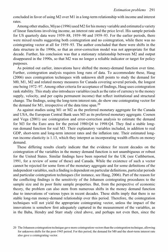
Estimation problems 291
concluded in favor of using M2 over M1 in a long-term relationship with income and interestrates.
Among other studies, Miyao (1996) used M2 for his money variable and estimated a varietyof linear functions involving income, an interest rate and the price level. His sample periodsfor US quarterly data were 1959–88, 1959–90 and 1959–93. For the earlier periods, therewere mixed results suggesting both cointegration and no cointegration, while there was nocointegrating vector at all for 1959–93. The author concluded that there were shifts in thedata structure in the 1990s, so that an error-correction model was not appropriate for thatdecade. Further, his conclusion was that a stationary relationship between M2 and outputdisappeared in the 1990s, so that M2 was no longer a reliable indicator or target for policypurposes.
As pointed out earlier, innovations have shifted the money-demand function over time.Further, cointegration analysis requires long runs of data. To accommodate these, Haug(2006) uses cointegration techniques with unknown shift points to study the demand forM0, M1, M2 and related money measures for Canada covering several periods, the longestone being 1972–97. Among other criteria for acceptance of findings, Haug uses cointegrationrank stability. This study also introduces variables (such as the ratio of currency to the moneysupply, velocity, and per capita permanent income) that reflect institutional and structuralchange. The findings, using the long-term interest rate, do show one cointegrating vector forthe demand for M1, irrespective of the data time span.20
As against studies using M1 or M2 as the preferred monetary aggregate for the Canadaand USA, the European Central Bank uses M3 as its preferred monetary aggregate. Coenenand Vega (2001) use cointegration and error-correction analysis to estimate the demandfor M3 for the Euro area for the period 1980:Q4 to 1998:Q4. They find a stable long-run demand function for real M3. Their explanatory variables included, in addition to realGDP, short-term and long-term interest rates and the inflation rate. Their estimated long-run income elasticity is 1.13, which they interpret as incorporating wealth effects on moneydemand.
These differing results clearly indicate that the evidence for recent decades on thecointegration of the variables in the money demand function is not unambiguous or robustfor the United States. Similar findings have been reported for the UK (see Cuthbertson,1991, for a review of some of these) and Canada. While the existence of such a vectorcannot be rejected for some form of the monetary aggregate and for some definitions of theindependent variables, such a finding is dependent on particular definitions, particular periodsand particular cointegration techniques (for instance, see Haug, 2006). Part of the reason forthe conflicting findings is the sensitivity of the Johansen cointegrating procedures to thesample size and its poor finite sample properties. But, from the perspective of economictheory, the problem can also stem from numerous shifts in the money demand functiondue to innovations of various types in recent decades. These shifts imply that there is nostable long-run money-demand relationship over this period. Therefore, the cointegrationtechniques will not yield the appropriate cointegrating vector, unless the impact of theinnovations is somehow first adequately captured in the measurement of the variables, asin the Baba, Hendry and Starr study cited above, and perhaps not even then, since the
20 The Johansen cointegration technique gave more cointegration vectors than the cointegration technique, allowingfor unknown shifts for the post-1945 period. For this period, the demand for M0 and the short-term interest ratealso gave a cointegrating vector.

292 The demand for money
innovations have been of numerous types and their collective combination has itself beenchanging.
9.9 Causality
Since the ECM incorporates lags of the explanatory and other exogenous variables onthe right-hand side, its estimates are often used to determine the direction of Grangercausality. The criteria for judging one-way versus two-way Granger causality were specifiedin Chapter 7.
9.10 An illustration: money demand elasticities in a periodof innovation
Table 9.1 provides an illustration of the estimates of money demand with a lagged dependentvariable and is based on Goldfeld and Sichel (1990). Part of this table is based on Fair (1987),who presented the estimates of money demand for 27 countries.
Income elasticities in Table 9.1
In Table 9.1, the coefficient of the income variable y is the impact elasticity for the quarterand lies in the range 0.039 to 0.118. The long-run elasticity is obtained by dividing theimpact elasticity by one minus the coefficient of the lagged dependent variable m−1. Thecomputation of long-run elasticity becomes extremely sensitive to small changes as thiscoefficient approaches one. In fact, if this coefficient is one or over one, the partial adjustmentmodel leads to a misspecification in its adjustment mechanism. This is clearly so for theUSA for 1952:3–1979:3, and almost so for 1974:2–1986:4. The estimates for these periodstherefore cannot be relied upon, as a look at the long-run income and interest-rate elasticitiesclearly shows.
Table 9.1 Estimates of money demand
Country Sample period y R1 R2 π m−1 Long-run elasticities
Income Interestc
USAa 1952:3–1974:1 0.131 −0.016 −0.030 −0.771 0.788 0.62 −0.0751952:3–1979:3 0.039 −0.013 −0.002 −0.889 1.007 −5.57 1.8571974:2–1986:4 0.044 −0.018 0.100 −0.823 0.997 14.67 −6
Canadab 1962:1–1985:4 0.071 −0.004 −1.66 0.94 1.18 −0.067UKb 1958:1–1986:1 0.118 −0.005 −0.69 0.44 0.21 −0.009
Source: Goldfeld and Sichel (1990), Tables 8.1 and 8.5, of which Table 8.5 is based on Fair (1987).
Notesa All variables are in logs, except for the inflation rate π (= ln(Pt/Pt−1)). The dependent variable — is real money
balances m, measured by the real value of M1, and y is real GNP. R1 is the commercial paper rate and R2 is thepassbook savings rate at commercial banks.
b All variables are in logs except the interest rate R1 which is in levels. The dependent variable m is real balancesper capita and the scale variable is income per capita. r1 is a short-term rate. The reported estimates are takenfrom Goldfeld and Sichel (1990), Table 8.5, calculated by them from Fair (1987).
c Based on the coefficient of R1.
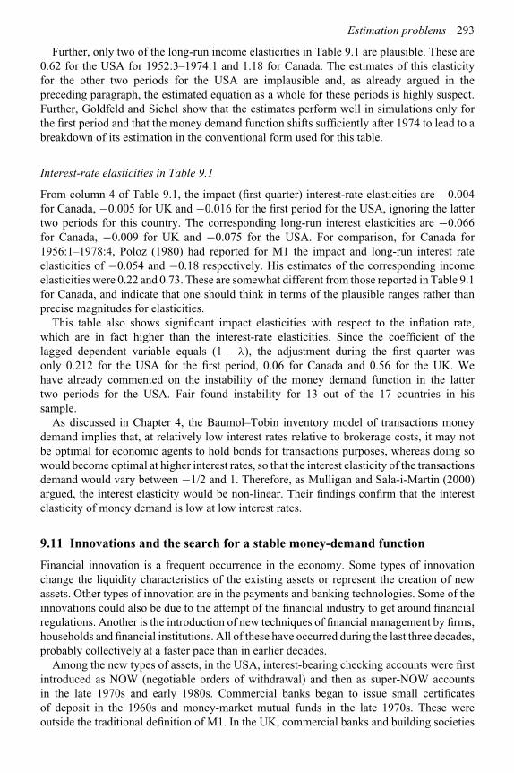
Estimation problems 293
Further, only two of the long-run income elasticities in Table 9.1 are plausible. These are0.62 for the USA for 1952:3–1974:1 and 1.18 for Canada. The estimates of this elasticityfor the other two periods for the USA are implausible and, as already argued in thepreceding paragraph, the estimated equation as a whole for these periods is highly suspect.Further, Goldfeld and Sichel show that the estimates perform well in simulations only forthe first period and that the money demand function shifts sufficiently after 1974 to lead to abreakdown of its estimation in the conventional form used for this table.
Interest-rate elasticities in Table 9.1
From column 4 of Table 9.1, the impact (first quarter) interest-rate elasticities are −0.004for Canada, −0.005 for UK and −0.016 for the first period for the USA, ignoring the lattertwo periods for this country. The corresponding long-run interest elasticities are −0.066for Canada, −0.009 for UK and −0.075 for the USA. For comparison, for Canada for1956:1–1978:4, Poloz (1980) had reported for M1 the impact and long-run interest rateelasticities of −0.054 and −0.18 respectively. His estimates of the corresponding incomeelasticities were 0.22 and 0.73. These are somewhat different from those reported in Table 9.1for Canada, and indicate that one should think in terms of the plausible ranges rather thanprecise magnitudes for elasticities.
This table also shows significant impact elasticities with respect to the inflation rate,which are in fact higher than the interest-rate elasticities. Since the coefficient of thelagged dependent variable equals (1 − λ), the adjustment during the first quarter wasonly 0.212 for the USA for the first period, 0.06 for Canada and 0.56 for the UK. Wehave already commented on the instability of the money demand function in the lattertwo periods for the USA. Fair found instability for 13 out of the 17 countries in hissample.
As discussed in Chapter 4, the Baumol–Tobin inventory model of transactions moneydemand implies that, at relatively low interest rates relative to brokerage costs, it may notbe optimal for economic agents to hold bonds for transactions purposes, whereas doing sowould become optimal at higher interest rates, so that the interest elasticity of the transactionsdemand would vary between −1/2 and 1. Therefore, as Mulligan and Sala-i-Martin (2000)argued, the interest elasticity would be non-linear. Their findings confirm that the interestelasticity of money demand is low at low interest rates.
9.11 Innovations and the search for a stable money-demand function
Financial innovation is a frequent occurrence in the economy. Some types of innovationchange the liquidity characteristics of the existing assets or represent the creation of newassets. Other types of innovation are in the payments and banking technologies. Some of theinnovations could also be due to the attempt of the financial industry to get around financialregulations. Another is the introduction of new techniques of financial management by firms,households and financial institutions. All of these have occurred during the last three decades,probably collectively at a faster pace than in earlier decades.
Among the new types of assets, in the USA, interest-bearing checking accounts were firstintroduced as NOW (negotiable orders of withdrawal) and then as super-NOW accountsin the late 1970s and early 1980s. Commercial banks began to issue small certificatesof deposit in the 1960s and money-market mutual funds in the late 1970s. These wereoutside the traditional definition of M1. In the UK, commercial banks and building societies
294 The demand for money
introduced checkable interest-bearing accounts in the 1980s. In each case, there was alearning period for the public and shifts in the money demand function were evident overmany years.
If the innovations merely change the constant term or the coefficients of the independentvariables in the money demand function, they can be relatively easy to capture in estimationthrough period splitting or the use of dummy constant and interactive variables. However,some of the resulting shifts of the money demand function are much more difficult to captureor cannot be captured, and the researcher ends up with the judgment that the money demandfunction has become unstable.
The desperate search for a stable money demand function
The last three decades have seen a remarkable number of innovations in the monetarysphere. These have resulted in a breakdown of the estimated money demand functionsand a large number of innovations by researchers in their estimating equations andtechniques. The attempts to find a stable demand function have included changes inthe monetary aggregate used as the dependent variable (M1, M2, M3, or their Divisiacounterparts). Other attempts have centered around variations in the arguments of thefunction. These included the use of current income, permanent income, wage income orproperty income, etc., for the scale variable, and the use of short interest rates, long interestrates, the rate of inflation or a composite index of interest rates, etc., for the interest ratevariable.
Still other attempts changed the form of the estimating equation from linear to log-linear andsemi-log-linear, or switched to non-linear functions or tried ones with stochastic coefficients,or used transcendental functions. Some other attempts focused on the proper specification ofthe dynamic adjustment of the actual to desired money balances. The econometric techniqueshave included the classical regression techniques and cointegration–error-correction models,among others.
This prolific variety of attempts and deviations from the standard money demand equationalmost gives one the impression of a field dominated by data mining and the ad hocconstructions of a profession desperate to find a stable money demand function to backits theory. While this may sound a rather harsh assessment, it does serve as a reminder of thesevere difficulties in finding a stable money demand function during the ongoing innovationsof the recent decades.
For the USA, there appears to have been a downward shift in the demand function duringthe 1970s and an upward shift during the 1980s. In these decades, as in the 1990s, actualmoney holdings deviated remarkably from the predictions of most estimated money demandmodels. In terms of velocity, the velocity of M1 increased in the 1970s and decreased in the1980s in a manner not predicted by these models.
Conclusions
Empirical findings generally confirm the homogeneity of degree zero of the demand forreal balances with respect to the price level – and the consequent homogeneity of degreeone of the demand for nominal balances – as discussed in Chapter 3. The income elasticityof real M1 with respect to real income has been established as being less than one, evenin the long run, though some studies show the income elasticity for real M2 to be evenslightly larger than unity. The latter is particularly so for developing economies, in which the
Estimation problems 295
bond and stock markets are not well developed, so that increases in savings are mostlyheld in savings deposits. Real balances do depend on interest rates, with a short-termrate being usually used in the estimation of M1 demand and a longer term one beingused for the estimation of M2 demand. The estimated interest-rate elasticities usually fallin the range from −0.15 to −0.50. In the LDCs, the rate of inflation typically performsbetter in estimation than the rate of interest and is often used in lieu of the latter, withsomewhat similar elasticities. While currency substitution is a theoretical possibility andsome studies do confirm its existence for their data sets, empirical studies have not alwaysfound it to be so significant that the elimination of the return on foreign currencies fromthe money demand function leads to much worse results. Most money demand functionsare, therefore, estimated without this variable. Not much support has been found forthe liquidity trap and it is now hardly ever investigated or even mentioned in empiricalstudies.
The velocity of circulation of M1 is not a constant in either the short or the long run. In theshort run, its annual variation is quite significant even in stable economies without politicaland economic panics. It is about 3 percent to 4 percent for the USA, but can be much higherin less stable economies. Since the income elasticity of M1 is likely to be less than one in thelong run, the long-run expectation for its velocity is that it will increase.
Innovations in the financial sector and in the usage of money by non-financial economicagents in the economy have been very rapid in the last three decades, so that the moneydemand functions estimated with data including this period are often not stable. Further, it iseven more rare to find the estimated functions for both narrow and wide definitions of moneyto be stable for a given country over a given period.
For the open economy, the existence of extensive CS could cause the monetary authority tolose control of the domestic money supply and increase the volatility of exchange rates undera floating exchange rate regime. It would increase the speculative pressures under fixedexchange rates. A common finding in estimations of the open-economy domestic moneydemand function is that the expected change in the exchange rate – which is the proxy on thereturn on holding foreign money relative to that on domestic money – is not significant inexplaining domestic money demand. Such a finding has led to the conclusion that currencysubstitution tends to be extremely low, even in countries like Canada, in which the public oftenholds US dollars in currency or in US dollar bank deposit accounts. However, many studiesalso show that the return on foreign bonds is a significant positive determinant of domesticmoney demand. This could provide indirect evidence on CS: if foreign money balancesprovide monetary services as a medium of payments in the domestic economy, the decreasein their holdings due to an increase in the return on foreign bonds, has to be compensated byan increase in domestic money balances in order to maintain the desired holdings of all mediaof payments. This effect relies on the substitution between the domestic and foreign monies intheir medium-of-payments role, while relying upon substitution between the foreign moneyand foreign bonds in portfolio allocation.
Several of the variables crucial to money demand estimation are not stationary. Thisis especially likely to be so for the monetary aggregates themselves, as well as for theincome and wealth variables. It may or may not also be so for the interest rates in theparticular data set. Consequently, the classical regression techniques do not yield unbiasedand consistent coefficients. Cointegration analysis is an appropriate procedure in this caseand has become quite common in recent years for estimating money demand functions. Itscombination with error-correction modeling has the further advantage that the estimationyields both the long-run and the short-run demand functions.
296 The demand for money
Cointegration procedures represent an attempt to capture the long-run equilibriumrelationship and there should exist a cointegrating vector if such a relationship is stable overthe sample period. However, when long-run relationships are shifting due to innovations andthe impact of the innovations has not been eliminated or somehow captured in the definitionof the variables or the procedure used, the sample data would not incorporate a stable long-runrelationship.
Money demand studies using cointegration techniques for data over the last few decadeshave provided a mixed bag of evidence about the existence of a cointegrating vectorbetween money, income, interest rates and prices. The finding of such a vector has oftenbeen culled from the data by using different definitions of money, different interest ratesand different periods. The last few decades have seen a mixed bag of very significantinnovations related to money demand, so that the long-run money demand function musthave been shifting. Consequently, cointegration studies, like earlier studies using thestandard regression techniques, have not provided convincing evidence of the existence ofa stable long-run money-demand function for the last few decades for Britain, Canada andthe USA.
In studies where acceptable cointegration vectors have been established, an error-correctionmodel has usually also been estimated. As expected, these studies show for quarterly datathat the impact elasticities are relatively quite small and much smaller than the long-runelasticities, indicating that adjustments of money demand to changes in the independentvariables take at least several quarters.
We have not differentiated between the demand functions estimated for the differentsegments of the economy, such as households, firms and financial institutions. There arenumerous studies on these and the interested reader is encouraged to explore them. Thereis a significant difference between the demand for money by households and that by firms,especially large ones. In general, the former tends to be relatively more predictable than thelatter.
Summary of critical conclusions
❖ The income elasticity of the demand for M1 is less than one.❖ The income elasticity of M2 demand is higher than that of M1 demand and is sometimes
estimated to be greater than one.❖ The negative interest elasticity of the demand for money, no matter how it is defined, is
now beyond dispute.❖ Empirical studies do not show convincing evidence of the liquidity trap, even for data
covering the 1930s.❖ M1 has performed better than broader monetary aggregates during some periods and worse
in others. Several recent studies have supported the use of M1 over M2 and broaderaggregates.
❖ For the 1960s and 1970s, estimates based on a partial adjustment model often indicated alow impact (income) elasticity for the first quarter but a long-run elasticity close to one,indicating a slow adjustment of money demand to its long-run level.
❖ Financial innovations during the last three decades have rendered the money demandfunction unstable for this period. Numerous attempts and innovative variations in estimationhave not established a stable demand function, with a specific form and invariantcoefficients, for out-of-sample data.

Estimation problems 297
❖ Most of the variables relevant to the money demand function have proved to be non-stationary. Therefore, most empirical studies now use cointegration analysis with an error-correction model. The latter is also used to judge causality between money and output.
Appendix
The ARDL model and its cointegration and ECM forms
As explained in Chapter 8, the regressors in an autoregressive distributed lag (ARDL) modelinclude the lagged values of the dependent variable and the current and lagged values ofthe explanatory variables. Its estimating equation with p lagged values of the dependentvariable and qj, j = 1,2, . . .,n, values of the n explanatory variables is designated as anARDL(p,q1, . . .,qn) and has the form:
β(L,p)yt = β0x0 +n∑
j=1
βj(L,q)xjt +μt (32)
where L is the lag operator such that Liyi = yt−i, x0 is a constant and (L, p) and (L, q) are thelag polynomials:
α(L,p) = 1 −α1L1 −α2L2 −αpLp (33)
β(L,q) = 1 −β1L1 −β2L2 −αqLq (33′)
In the long run, yt = yt−1 = ·· · = yt−p and xjt = xjt−1 = ·· · = xjt−q, so that L = 1, α(1,p) =(1 −α1 −α2 −αp) and β(1,q) = (1 −β1 −β2 −βq) and the long-run relationship becomes:
yt = β ′0 +
n∑j=1
β ′j x
′jt + νt (34)
where α′0 = α0/(α(1,p),βj = β ′
j (1,q)/(α(1,p),vj = μj/(α(1,p). The error-correction equa-tion of this ARDL model is:
�yt = �β ′0 −
p∑i=2
α′i�yt−i +
n∑j=1
β ′j0�xit −
n∑j=1
q∑i=2
β ′i,t−j�xj,t−i −α(1,p)ECMt−1 +ηt
(35)
where:
ECMt−1 = yt−1 − β −n∑
j=1
βjxjt−1 (36)
α(1, p) measures the speed of adjustment.

298 The demand for money
An illustration: a simple ARDL model
The simplest case of an ARDL model has only one explanatory variable x1 and one-periodlags, so that it is ARDL(1, 1). The estimation equation for this case is:
yt = α0 +α1yt−1 +β0x1t +β1x1t−1 +μt (37)
where μ is white noise. The long-run relation between y and x1 for this equation is obtainedby setting yt = yt−1 and xt = xt−1, so that the long-run equation is:
y = α0/(1 −α1) +{(β0 +β1)/(1 −α1)}x1t +{1/(1 −α1)}μt (38)
where (β0 + β1)/(1 − α1) provides the long-run relationship between y and x. Further, in(38), replacing yt by (yt−1 +�yt) and x1t by (x1t−1 +�x1t), we get:
�yt = α0 − (1 −α1)yt−1 +β0�x1t + (β0 +β1)x1t−1 + νt (39)
which is the short-run ECM representation of (37).Further, from (37), we have:
yt −α1yt−1 = α0 +β0x1t +β1x1t−1 +μt
(1 −α1L)yt = α0 +β0x1t +β1x1t−1 +μt
(40)
Expanding {1/(1 −α1L)}, we have:
1/(1 −α1L) = (1 +α1 +α 21 +·· ·)
Hence, (40) yields:
yt = (1 +α1 +α 21 +·· ·)α0 + (1 +α1 +α 2
1 +·· ·)(β0x1t +β1x1t−1 +μt) (41)
which is another way of stating (37). In this context, (1 + α1 + α21 + ·· · ) (β0 + β1) = (β0 +
β1)/(1 −α1)) provides the long-run relationship between y and x.
Review and discussion questions
1. Empirical studies of the demand for money in the last two or three decades have raisedserious doubts about the stability of the money demand function. What were the maincauses of this instability?
Was the finding of instability related to the particular monetary aggregate used or didit occur across all aggregates? What were the main modifications made in the estimatingequations and in the definitions of the variables in order to reach a stable money-demandfunction?
2. Specify the relevant relationships and discuss how the error-correction model can beused to assess causality between money and (i) nominal income, (ii) real output?
3. Specify the appropriate relationship and discuss the use of cointegration and error-correction estimates to judge (i) long-run, (ii) short-run neutrality of money.

Estimation problems 299
4. Specify the appropriate relationship and discuss whether the cointegration and error-correction estimates can shed any light on the question of whether the deviations of outputfrom its full-employment level are transitory and self-correcting, as the modern classicalmodel asserts. If they were not such as to imply transitory and self-correcting deviationsof output from its full-employment value, do they indicate any role for monetary policyto moderate these deviations?
5. How would you formulate your money demand function for estimation in an empiricalstudy? Comment on the a priori relationships that you expect between your independentvariables and money. Compare your demand function with some roughly similar andsome different ones estimated in the literature.
6. For a selected country and using quarterly data, specify and estimate the money demandfunction. Check and correct for shifts in this function during the period of your study.Try the following variations of the independent variables:
(i) Expected income and permanent income for the scale variable.(ii) Two different interest rates, one short-term and the other medium-term.(iii) A proxy for the expected change in the exchange rate.(iv) Also, do your estimations using the following techniques:
(a) least squares estimation, with a first-order PAM;(b) cointegration with an error-correction model.
(v) Discuss your choice of the functional form of the money demand function and yourchoice of the variables and the econometric techniques used, as well as the data andeconometric problems you encountered.
(vi) Discuss your results, their plausibility and consistency with the theory, and theirrobustness.
7. Discuss: shifts in the estimated coefficients of the money demand function are aslikely to be due to shifts in monetary policy (supply side shifts) as about moneydemand behavior. (This question relates to the identification of demand versus supplyfunctions.)
8. What are the reasons for requiring the use of cointegration techniques in money demandestimation? What would be the disadvantages of using ordinary least squares for suchestimation? If you use both and obtain different estimates, which would you rely on, andwhy?
9. Are there any conceptual problems with the application of the cointegration techniques tomoney-demand functions, or can the estimates from such techniques be relied upon? Inparticular, how can you make certain that the estimated cointegration vector is the moneydemand and not the money supply function or a reduced-form relationship betweenmoney demand and money supply?
10. Specify the Taylor rule. Discuss its estimation by cointegration and error-correctiontechniques, specifying and justifying your choices of the dependent and explanatoryvariables.
11. In the context of interest-rate targeting (as against monetary targeting), suppose youwanted to estimate a St Louis equation for (i) nominal income, (ii) real output, butwith the interest rate as the monetary policy variable. Specify the appropriate equation.Discuss its estimation by cointegration and error-correction techniques.
12. Conduct an empirical study along the lines suggested in the preceding question for acountry of your choice, and discuss your findings for the effectiveness of monetarypolicy pursued through interest rates.

300 The demand for money
13. Design a study to judge whether a central bank of a country uses the interest rate or themoney supply as its operating target of monetary policy. What relationships and testscan you use for this purpose?
References
Baba, Y., Hendry, D.F., and Starr, R.M. “The demand for M1 in the U.S.A., 1960–1988.” Review ofEconomic Studies, 59, 1992, pp. 25–61.
Bae, Y., Kakkar, V., and Ogaki, M. “Money demand in Japan and nonlinear cointegration.” Journal ofMoney, Credit and Banking, 38, 2006, pp. 1659–67.
Coenen, G., and Vega, J.L. “The demand for M3 in the Euro area.” Journal of Applied Econometrics,16, 2001, pp. 727–48.
Cuthbertson, K. “Modelling the demand for money.” In C.J. Green and D.T. Llewellyn, eds, Surveysin Monetary Economics, Vol. 2. Cambridge, MA: Blackwell, 1991.
Davidson, R., and Mackinnon, J.G. Estimation and Inference in Econometrics. New York: OxfordUniversity Press, 1993.
Engle, R.F., and Granger, C.W.J. “Cointegration and error-correction: representation, estimation andtesting.” Econometrica, 55, 1987, pp. 251–76.
Fair, R.C. “International evidence on the demand for money.” Review of Economics and Statistics, 69,1987, pp. 473–90.
Feige, E.L. “Expectations and adjustments in the monetary sector.” American Economic Review, 57,1967, pp. 462–73.
Feige, E.L., and Pearce, D.K. “The substitutability of money and near-monies: a survey of the time-seriesevidence.” Journal of Economic Literature, 15, 1977, pp. 439–70.
Goldfeld, S.M. “The demand for money revisited.” Brookings Papers on Economic Activity, 3, l973,pp. 576–638.
Goldfeld, S.M., and Sichel, D.E. “The demand for money.” In B.M. Friedman and F.H. Hahn,eds, Handbook of Monetary Economics. Amsterdam: North-Holland, 1990, Volume 1, Chapter 8,pp. 299–356.
Hafer, R.W., and Jansen, D.W. “The demand for money in the United States: evidence fromcointegration tests.” Journal of Money, Credit and Banking, 23, 1991, pp. 155–68.
Haug, A.A. “Canadian money demand functions: cointegration-rank stability.” The Manchester School,74, March 2006, pp. 214–30.
Johansen, S. “Statistical analysis of cointegration vector.” Journal of Economic Dynamics and Control,12, 1988, pp. 231–54.
Johansen, S. “Estimation and hypothesis testing of cointegration vectors in Gaussian vectorautoregressive models.” Econometrica, 59, 1991, pp. 1551–80.
Johansen, S., and Juselius, K. “Maximum likelihood estimation and inference on cointegration withapplication to the demand for money.” Oxford Bulletin of Economics and Statistics, 52, 1990,pp. 169–210.
Judd, J.P., and Scadding, J.L. “The search for stable money demand function: a survey of the post-1973literature.” Journal of Economic Literature, 20, 1982, pp. 993–1023.
Keynes, J.M. The General Theory of Employment, Interest and Money. London and New York:Macmillan, 1936.
Miller, S.M. “Money dynamics: an application of cointegration and error-correction modeling.” Journalof Money, Credit and Banking, 23, 1991, pp. 139–54.
Miyao, R. “Does a cointegrating M2 demand relation really exist in the United States?” Journal ofMoney, Credit and Banking, 28, 1996, pp. 365–80.
Mulligan, C., and Sala-i-Martin, X. “Extensive margins and the demand for money at low interestrates.” Journal of Political Economy, 108, 2000, pp. 961–91.
Pesaran, M.H., Shin, Y., and Smith, R.J. “Bounds testing approaches to the analysis of levelrelationships.” Journal of Applied Econometrics, 16, 2001, 289–326.

Estimation problems 301
Poloz, S.S. “Simultaneity and the demand for money in Canada.” Canadian Journal of Economics, 13,1980, pp. 407–20.
Sriram, S.S. “Survey of literature on demand for money: theoretical and empirical work with specialreference to error-correction models.” IMF Working Paper no. 64, 1999.
Sriram, S.S. “A survey of recent empirical money demand studies.” IMF Staff Papers, 47, 2000, 334–65.


Part IV
Monetary policy and centralbanking


10 Money supply, interest rates and theoperating targets of monetary policyMoney supply and interest rates
This is the first of three interrelated chapters on monetary policy and central banking. It startsby examining the goals and operating targets of monetary policy. The two major operatingtargets of monetary policy are the money supply and the interest rate.
This chapter then focuses on the determination of the money supply. While macroeconomicmodels tend to simplify by assuming that the money supply is exogenously determined, theprivate sector in the form of the banks, households and firms also influences the moneysupply.
Key concepts introduced in this chapter
♦ Targeting inflation or its deviation from a desired inflation rate♦ Targeting output and unemployment♦ Interest rate as an operating target♦ Monetary base♦ Currency ratio♦ Demand deposit ratio♦ Free reserves♦ Excess reserves♦ Required reserves♦ Discount/bank rate♦ Mechanical theories of the money supply♦ Behavioral theories of the money supply
This is one of three chapters on some of the central issues of monetary policy. It starts withthe relationships among the goals, intermediate targets and operating targets of monetarypolicy and examines the theoretical justification as well as the implications of adoptingdifferent targets. It then considers the issue of whether the central bank should use the moneysupply or the interest rate as its major monetary policy instrument. It then narrows its focusto the determination of the money supply in the economy, so as to complement the extensivetreatment of money demand in the preceding chapters.
Sections 10.1 and 10.2 present the links between the goals and targets of monetary policy.Sections 10.3 to 10.5 examine the main operating targets of monetary policy commonly

306 Monetary policy and central banking
used by central banks and their justification from macroeconomic analysis.1 Sections 10.6to 10.8 present the determination of the money supply. Section 10.9 covers the applicationof cointegration analysis and error-correction modeling to money supply. Section 10.10considers the central bank’s choice between the monetary base and the interest rate asalternative operating targets.
Stylized facts on the goals and operating targets of monetary policy
The stylized facts on monetary policy depend on the behavior of the central bank and thestructure of the economy. Among these facts are:
1 The central bank has more than one goal. Among its goal variables are output andits growth rate, unemployment, inflation, etc. Currently many central banks focus onreducing the deviation of output from its full-employment level and of inflation from atarget level, with a trade-off between them, as in a Taylor rule.
2 The target inflation rate for many central banks now is a low inflation rate, often in arange of 1 percent to 3 percent.
3 The operating target of monetary policy can be a monetary aggregate or an interest rate.A monetary aggregate was selected for this purpose in some past periods and is still inuse by some central banks. Currently, many central banks in the developed economiesfocus on an interest rate as their primary operating target.
4 The central bank does not control the money supply directly but has to use its instruments,such as the monetary base, for indirectly controlling the money supply.
10.1 Goals, targets and instruments of monetary policy
The eventual purpose of monetary policy is to achieve certain national goals. These havehistorically included full employment (or a low unemployment rate), full-employment output(or a high output growth rate), a stable price level (or a low inflation rate), a stable exchangerate (or a desirable balance of payments position), etc. These variables are simply referredto as “goals” or as “ultimate goals” of monetary policy. However, the central bank cannotachieve these goals directly by its monetary policy instruments, which are variables thatit can operate on directly. Among the instruments available to the central bank are open-market operations and changes in its discount/bank rate at which it lends to commercialbanks and other bodies. These determine the economy’s monetary base. In many countries,the central bank can also change the required reserves (i.e. the minimum reserves thecommercial banks must hold against the public’s deposits with them), which changes the“monetary base multiplier” (i.e. the money supply per dollar of the monetary base). Thesemeasures serve to change the money supply in the economy. Another monetary policyinstrument is the overnight loan rate (called the federal funds rate in the USA) in the marketfor reserves, whose operation induces change in various interest rates in the economy.The next chapter provides further information on the goals and instruments of monetarypolicy.
1 This section requires some prior knowledge of the IS–LM and IS–IRT models of aggregate demand frommacroeconomic courses. A review of these models is provided in Chapter 13.

Operating targets 307
Besides the concepts of goals and instruments, other concepts relevant to monetary policyare those of targets, operating targets and guides. We can broadly define a target variable asone whose value the policy maker wants to change.2 An operating target variable is one onwhich the central bank can directly or almost directly operate through the instruments at itsdisposal. A guide is a variable that provides information on the current and future state ofthe economy.
Between the goals and instruments of monetary policy lie layers of intervening variables.For example, suppose the central bank wants to reduce the inflation rate. To do so, it needsto reduce aggregate demand in the economy. The reduction in aggregate demand usuallyrequires a reduction in investment and/or consumption, which requires an increase in marketinterest rates. Depending on the analysis, discussion or author, these intervening variables canbe referred to as intermediate targets, operating targets or even as instruments. Since a targetvariable is one whose value the central bank seeks to influence or control by the use of thetools at its disposal, any of the intervening variables between the goals and instruments can bereferred to as a target variable. In the preceding example, aggregate demand is an intermediatevariable or target, which the central bank wants to alter by using the intermediate targets of themoney supply and/or interest rates which, in turn, can be altered by changes in the monetarybase and the discount rate. Note that the word “target” can also be used to indicate a desirablevalue of a goal (e.g. inflation) or of an intermediate variable (e.g. the money supply andmarket interest rates).
Given the preceding discussion, Table 10.1 provides a rough classification of monetarypolicy instruments, operating targets, intermediate targets and goals.
While Table 10.1 provides some guidance on the roles and sequence of the variousmonetary policy variables, there is no hard and fast rule for its classification. The central bankuses its tools to hit its operating targets, with the intention of manipulating the intermediatetargets, which are the final ones of the financial system, in order to achieve its goals. Notethat lags enter at each stage of this process, and both the individual lag and the overall lagtend to vary. Further, the duration of the lags and the final impact are not usually totallypredictable.
Table 10.1 Monetary policy tools, target and goals
Policy instruments Operating targets Intermediate targets Goals
Open-market operationsDiscount rateReserve requirements
Short-term interest ratesReserve aggregates
(monetary base,reserve, nonborrowedreserves, etc.)
Monetary aggregates(M1, M2, etc.)
Interest rates (shortand long term)
Aggregate demand
Low unemploymentrate
Low inflation rateFinancial market
stabilityExchange rates
2 Under this broad definition, targets can be ultimate ones (final goals, such as output and unemployment),intermediate ones (such as the money supply or the interest rate) or operating ones (such as the monetary baseor the discount rate). Since a given variable can fall in any one of these categories, there is no hard and clear-cutseparation between these categories.
308 Monetary policy and central banking
10.2 Relationship between goals, targets and instruments,and difficulties in the pursuit of monetary policy
Several issues arise in the selection and use of goals, intermediate variables and operatingtargets or instruments by the monetary authorities. Among these are:
1 Are the relationships between the ultimate goal variables, intermediate variables andoperating targets stable and predictable?
2 Can the central bank achieve the desired levels of the operating targets through theinstruments at its disposal?
3 What are the lags in these relationships, and, if they are long, can the future course ofthe economy be reasonably well predicted?
To illustrate these points, let the relevant relationships be:
y = f (x;Ψ ) (1)
x = g(z;θ ) (2)
where:y = (ultimate) goal variablex = intermediate targetz = policy instrument or operating targetΨ,θ = sets of exogenous variables
The above equations imply that:
y = h(z;Ψ,θ ) (3)
so that z can be used to achieve a desired value of y. However, this can be done reliablyonly if the functional forms f and g are known and these are stable univalued functions.3 Inpractice, given the complex structure of the real-world economies, as well as the existenceof uncertainty and lags in the actual relationships, the precise forms of f, g and h are oftenonly imperfectly known at the time the decisions are made. Further, the coefficients in theserelationships may be subject to stochastic changes. In addition, given the lags in the economy,the policy maker also needs to predict the future values of the coefficients and the exogenousvariables – again, usually an imprecise art.
Hence, the precision and clarity implied by (3) for the formulation of monetary policy andits effects is misleading. In many, if not most instances, the impact of a change in most ofthe potential operating variables on the ultimate goals is likely to be imprecise, difficult topredict and/or unstable. This makes the formulation of monetary policy an art rather than ascience and cautions against attempts to use monetary policy as a precise control mechanismfor “fine-tuning” the goals of such policy.
Another common problem with most target variables is that they are endogenous and theirvalues depend on both demand and supply factors, so that the exogenous shocks to themcould come from either demand or supply shifts. The policy maker may want to offset theeffect of changes in some of these factors but not in all cases, so that it needs to know thesource of such changes before formulating its policy.
3 See also Chapters 9, 14–17 for material relevant to this discussion.
Operating targets 309
10.3 Targets of monetary policy
The two main operating targets usually suggested for monetary policy are:
• monetary aggregates;• interest rates.
The two main targets of monetary policy highlighted in the recent literature are:
• inflation rate (or the price level),4 or its deviation from a desired value;• output, or its deviation from the full-employment level.
There are also other variables that are sometimes used or proposed as the intermediatetargets of monetary policy. Among these is aggregate demand (or nominal national income)and, in the case of relatively open economies, the exchange rate or the balance of payments.For the sake of brevity, this chapter discusses only the relative merits and demerits of monetaryaggregates and the interest rate as the chief operating target or instruments. It also presentssome discussion of the price level and the inflation rate, and the output gap, as the targets ofmonetary policy.
10.4 Monetary aggregates versus interest rates as operating targets
This section relies upon students’ prior knowledge of the IS–LM macroeconomic model(otherwise, see Chapter 13) to distinguish between the relative merits of using the moneysupply versus interest rates as the operating target of monetary policy. The choice betweenmonetary aggregates and the interest rate depends critically upon the policy objective of thecentral bank and the structure of the economy. The following analysis, adapted5 from thatin Poole (1970), takes this objective to be control of aggregate demand,6 since the centralbank can only influence output and inflation, which are its final goal variables, throughmanipulation of aggregate demand. It further assumes that the structure of the economy canbe represented by the IS–LM analysis and diagram. This diagram has aggregate real demandy on its horizontal axis and the real interest rate r on its vertical axis. The commodity marketequilibrium is shown by the IS curve and the money market equilibrium is shown by theLM curve. Their intersection determines real aggregate demand at the existing price level.
4 Price stability is also sometimes designated as a primary policy goal. However, even in such a context, thejustification given for it is that price stability promotes the achievement of full employment and output growth.
5 This adaptation takes the control of aggregate demand rather than that of real output as the objective of monetarypolicy. Poole had treated the two as identical under the assumption that the price level was constant. Since thisassumption is both unnecessary and unrealistic, our discussion is based on the objective of minimizing the varianceof aggregate demand rather than of output.
6 However, note that the literature does also include other goal variables. One of these is the variance of themoney supply, with the choice between the monetary base and the interest rate depending on which instrumentminimizes this variance under shocks to money demand and money supply. In this analysis, when the interestrate is the policy instrument and the money supply is accommodated to money demand, shocks to both moneydemand and money supply affect the money supply. However, when the monetary base is the policy instrument,only the shock to the monetary base (to money supply) multiplier determines fluctuations in the money supply.Therefore, controlling the monetary base leads to smaller fluctuations in the money supply. We do not regard theobjective of minimizing the variance of money supply to be an appropriate goal, and do not present the analysisrelated to it.

310 Monetary policy and central banking
Therefore, the choice between the monetary instruments hinges on the question: whichinstrument provides better control over aggregate demand in the IS–LM framework? Ouranalysis implicitly assumes the Fisher equation for perfect capital markets and an expectedinflation rate of zero, so that the nominal interest rate R is identical with the real interestrate r.
Since the IS–LM analysis has not yet been mathematically covered in this book, thischapter presents only the diagrammatic analyses of monetary versus interest rate targeting.Its mathematical version is presented in Chapter 13, which could be read at this point.
10.4.1 Diagrammatic analysis of the choice of the operating targetof monetary policy
Shocks arising from the commodity market
The IS equation and curve encompass the various components of expenditures, such asconsumption, investment, exports, fiscal deficits, etc., in the economy (see Chapter 13).Several of these are volatile, with investment often being the most volatile component ofexpenditures. Shifts in any of these components shift the IS curve in the IS–LM diagram.
Our analysis starts with the initial equilibrium shown by point a, with coordinates (r0, y0),in Figure 10.1a. Assume that the central bank targets the money supply and holds it constantthrough open market operations or by the use of some other instruments. Shocks to the IScurve7 would then change both r and y. To illustrate, if a positive shock shifts the IS curvefrom IS0 to IS1, aggregate demand will increase from y0 to y1 and the interest rate rise fromr0 to r1. Similarly, a negative shock, occurring, say, in the following period, which shifts theIS curve to IS2, will lower aggregate demand to y2 and the interest rate to r2.
Compare this result with the impact of the same shock if the interest rate had been targeted.This is shown in Figure 10.1b, where the interest rate is assumed to be held fixed by theauthorities at the target rate r0, where the underline indicates that it is exogenously set by thecentral bank. The shifts in the IS curve, first to IS1 and then to IS2, will produce movements
r
yIS
LM
IS2
IS1
y ′2 y0 y ′1
r0
r1
r0
r2
a
r
y IS0
LM
IS2
IS1
y2 y0 y1
(a) (b)
Figure 10.1
7 Shocks originating in the commodity market are to consumption, investment, exports and governmentexpenditures. Of these, investment is considered to be the most volatile element.

Operating targets 311
in aggregate demand, first to y′1 and then to y′
2. This fluctuation between y′1 and y′
2 is clearlygreater than between y1 and y2 in Figure 10.1a, so that targeting the interest rate producesgreater fluctuations in aggregate demand than money supply targeting if the exogenous shocksemanate from the commodity market. Note that such shocks do not produce changes in theinterest rate, since that is being held constant through monetary policy.
Shocks arising from the money market
Now assume that the exogenous shocks arise only in the money market while there are noshocks in the commodity market, so that the IS curve does not shift. Such exogenous shocksin the money market can be to either money demand or money supply, and shift the LMcurve.
Money supply targeting would stabilize the money supply,8 so that disturbances to it donot have to be considered, but not the money demand. Now suppose that money demanddecreases. Given the targeted money supply, the decrease in the money demand will shift theLM curve in Figure 10.2 to the right to LM1 and increase aggregate demand from y0 to y1.Assume that the next period’s shock to the money demand increases it and shifts the LMcurve to LM2, so that aggregate demand falls to y2. The aggregate demand fluctuations arethen from y1 to y2 and the interest rate fluctuations are from r1 to r2.
For interest rate targeting, assume that the real interest rate had been set at r0, as shownin Figures 10.3 and 10.4. Figure 10.3 shows the initial demand curve for nominal balancesas M d and the initial supply curve as M s, with the initial equilibrium interest rate as r0 andthe initial money stock as M0. Now suppose that the money demand curve shifts from M d
0 toM d
1 . Since the interest rate is being maintained by the monetary authority at r0, the monetaryauthority will have to increase the money supplied from M0 to M1. The money stock thereforeadjusts endogenously through an accommodative monetary policy to the changes in moneydemand.
In the IS–LM Figure 10.4, a reduction in the money demand would shift the LM curveto the right from LM0 to LM1. However, given that the monetary authority maintains the
r
y
IS
LM
y2 y0 y1
r2
r0
r1
LM1
LM2
Figure 10.2
8 However, monetary base targeting usually will not do so.

312 Monetary policy and central banking
r
Md
r0
Md1
Ms0 Mst
MM1M0
Figure 10.3
y0
r2
r0
r1
r
y
IS
LM0
LM1
LM2
Figure 10.4
interest rate at r0, the aggregate demand y0 in this figure will be determined by the intersectionof the IS curve and a horizontal line at the target interest rate r0. This is so because theexogenous shift in the LM curve from LM0 to LM1 leads the central bank to undertake anaccommodative money supply decrease sufficient to shift this curve back to LM0. Hence, inspite of any exogenous changes in money demand, aggregate demand would remain at y0
(and the interest rate at r0). Hence, comparing the implications from Figures 10.2 and 10.4,monetary targeting will allow greater fluctuations in aggregate demand and interest rates thaninterest-rate targeting when the exogenous shifts arise from money demand.
This conclusion poses a problem for the policy maker since both types of shocks occur inthe real world. Therefore, the monetary authority has to determine the potential source of thedominant shocks to the economy before making the choice between monetary and interestrate targeting. This is not easy to determine for the future, nor need the same pattern of shocksnecessarily occur over time. Further, since both types of shock do occur, each policy willreduce or eliminate the impact of some types of shocks but not of others.
While many central banks had, for a few years during the late 1970s and sometimes in theearly 1980s, favored monetary targeting, the common practice currently is to set interest rates.
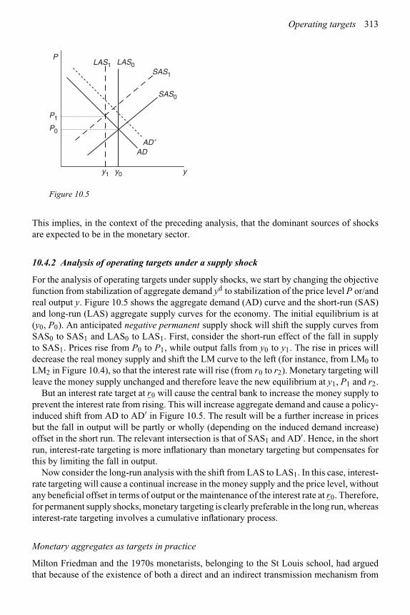
Operating targets 313
P
y1 y0 y
AD
SAS1
P1
P0
SAS0
LAS1 LAS0
AD ′
Figure 10.5
This implies, in the context of the preceding analysis, that the dominant sources of shocksare expected to be in the monetary sector.
10.4.2 Analysis of operating targets under a supply shock
For the analysis of operating targets under supply shocks, we start by changing the objectivefunction from stabilization of aggregate demand yd to stabilization of the price level P or/andreal output y. Figure 10.5 shows the aggregate demand (AD) curve and the short-run (SAS)and long-run (LAS) aggregate supply curves for the economy. The initial equilibrium is at(y0, P0). An anticipated negative permanent supply shock will shift the supply curves fromSAS0 to SAS1 and LAS0 to LAS1. First, consider the short-run effect of the fall in supplyto SAS1. Prices rise from P0 to P1, while output falls from y0 to y1. The rise in prices willdecrease the real money supply and shift the LM curve to the left (for instance, from LM0 toLM2 in Figure 10.4), so that the interest rate will rise (from r0 to r2). Monetary targeting willleave the money supply unchanged and therefore leave the new equilibrium at y1, P1 and r2.
But an interest rate target at r0 will cause the central bank to increase the money supply toprevent the interest rate from rising. This will increase aggregate demand and cause a policy-induced shift from AD to AD′ in Figure 10.5. The result will be a further increase in pricesbut the fall in output will be partly or wholly (depending on the induced demand increase)offset in the short run. The relevant intersection is that of SAS1 and AD′. Hence, in the shortrun, interest-rate targeting is more inflationary than monetary targeting but compensates forthis by limiting the fall in output.
Now consider the long-run analysis with the shift from LAS to LAS1. In this case, interest-rate targeting will cause a continual increase in the money supply and the price level, withoutany beneficial offset in terms of output or the maintenance of the interest rate at r0. Therefore,for permanent supply shocks, monetary targeting is clearly preferable in the long run, whereasinterest-rate targeting involves a cumulative inflationary process.
Monetary aggregates as targets in practice
Milton Friedman and the 1970s monetarists, belonging to the St Louis school, had arguedthat because of the existence of both a direct and an indirect transmission mechanism from

314 Monetary policy and central banking
the money supply to aggregate expenditures, the money supply rather than interest ratesprovided better control over the economy. Partly as an outcome of this advice, most countries –including the USA, Britain and Canada – switched to the targeting of monetary aggregatesafter the mid-1970s (though only until the early 1980s). The monetary aggregates oftensuggested as targets were M1 or M2 – and M4 in Britain – though sometimes even broadertargets were also considered.
Monetary aggregate targeting was predicated on the belief that the relationship betweensuch a target and aggregate demand was stable and had a short and predictable lag. Thiswas certainly the finding of the studies done by the St Louis school. Monetary targetswere pursued in the late 1970s and early 1980s by the monetary authorities in the USA,Canada and UK. However, the functional relationships between the monetary variables andaggregate expenditures, let alone the rate of inflation, proved to be unstable, so that theyhad been abandoned by the 1990s in each of these countries. Among the reasons for thisinstability were financial innovations and changes in the payments technology occurring inrecent decades.9 In terms of experience during the late 1970s and 1980s, direct targeting ofmonetary aggregates increased both the level and the volatility of interest rates considerably,with the latter considered by many economists to be destabilizing for the economy. Attemptsto control the monetary or reserve aggregates directly, as a way of controlling the economy,were abandoned by most central banks in the early 1980s in favor of interest-rate targets asthe control variable. This is not to say that the monetary aggregates are not monitored and thechanges in them not considered in formulating monetary policy. However, for most centralbanks, they have ceased to be the main operating targets.
Interest rates as targets in practice
Monetary policy acts through interest rates on spending, so that the interest rates are closerin the chain of influence on spending. Hence, they are more reliable and more appropriateindicators of the need for action than are the various measures of money supply and themonetary base. In line with this, in financially developed economies such as those of theUSA, Canada and the UK, the central banks believe that interest rates are a major indicatorof the performance of the economy and tend to use them as the preferred guide and operatingtarget of monetary policy.10
There are several measures of interest rates that may be considered, with the usual selectionfor operating purposes being of short-term nominal, rather than long-term or real, rates ofinterest. Historically, the measure commonly used for this purpose used to be the Treasurybill rate. As discussed later in Chapter 11, more recently the USA, UK and Canada have usedan overnight loan rate as an operating target. These countries have well-developed marketsfor overnight loans among financial institutions, with this market serving as the market forthe excess reserves of banks. This market for reserves is known as the Federal Funds marketin the United States and the overnight loan market in Canada and the UK. Such a rate reflectsthe commercial banks’ demand and supply conditions for reserves. The central bank’s policyactions on the monetary base immediately affect the commercial banks’ demand and supply
9 These financial innovations included the payment of interest on checking accounts and the increasing degree ofsubstitution between M1 and near-monies, telephone and on-line banking, etc.
10 In this context, see the discussion in Chapter 11 on the Monetary Conditions Index used by the Bank of Canada.
Operating targets 315
of reserves, thereby changing the overnight interest rate and starting a chain of reactions onother interest rates, and through these on the borrowing and lending, investment and consumerspending, etc., in the economy. A higher rate means that banks are relatively loaned up anda lower rate means that banks have relatively large free reserves, so that they can increaseloans of their own volition.
Problems with the use of interest rates in managing the economy
The observed interest rates are equilibrium rates, so that changes in them could reflecteither changes in demand or in supply conditions or both. Therefore, a rise in the interestrates may be due to an increase in the demand for loanable funds or a decrease in theirsupply, but the central bank may wish to take offsetting action in only one of thesecases. For example, interest rates rise during an upturn in the business cycle. The centralbank may not wish the upturn to be curbed by a decreased supply of funds but alsomay not wish to offset the stabilization effect of interest rates due to an increase in theirdemand. But changes in the equilibrium interest rates do not by themselves provide adequateinformation as to the causes of their rise and therefore as to the policy actions that shouldbe undertaken. Consequently, central banks in practice supplement information on interestrates with other information on demand and supply conditions before making their policydecisions.
A problem with using interest rates as an operational target is that the central bank candetermine the general level of interest rates but not equally well control the differentialsamong them. Examples of these differentials are the loan-deposit spread of commercialbanks, and the spread between deposit rates and mortgage rates, if the latter are variable.Spreads depend upon market forces and can be quite insensitive or invariant to the centralbank’s discount rate. Financial intermediation in the economy is more closely a function ofsuch differentials than of the level of interest rates, so that the ability of the central bank toinfluence the degree of financial intermediation through its discount rate and the overnightloan rate for reserves becomes diluted.
Among other problems is the lag in the impact of changes in the interest rate on aggregatedemand in the economy. Among the reasons for such lags are the costs of adjustment ofeconomic variables such as the capital stock and planned consumption expenditures, andthe indirect income effects of changes in interest rates. There are two aspects of this lag: itslength and variability. The former is often assessed at about six quarters to two years in theUnited States, Britain and Canada. While there is agreement that there is some variability inthe length of the lag, there is no consensus on whether it is so long that changes in interestrates, intended to be stabilizing, can prove to be destabilizing. Within the lag, the impact effect(within the same quarter) of interest rate changes on real aggregate demand is estimated tobe quite low, while the long-run effect is now believed to be very significant.
The actual use of interest rates for stabilization has often been found to be “too little,too late” – though this is usually a result of uncertainty about the need for and the lags inthe effects of monetary policy. This results in its cautious use, no matter what operationalor indicator variable is used. Given the duration of lags and the uncertainty at any timeabout the position of the economy in the business cycle, past experience does indicate thatcentral banks often change the interest rates later and in smaller steps than really needed. Aninitial change is, therefore, often followed by many more in the same direction over severalquarters.
316 Monetary policy and central banking
Money supply under an interest rate target
In market economies, the use by the central bank of the interest rate as its major instrument ofmonetary policy does not imply that it can ignore the money supply altogether. Interest ratesare determined in financial markets, so that if the central bank were to lower its interest rateand not provide the supporting required increase in the money supply, it would find that themarket rates will diverge from its desired ones, so that the intended effects on expenditureswill not be achieved. Hence, an interest-rate policy must be accompanied by an appropriatemoney supply. This topic is addressed in the macroeconomic context in Chapter 13.
10.5 The price level and inflation rate as targets
Targeting the price level
Current discussions of monetary policy often refer to inflation or price targeting as the goalof monetary policy. A stable price level or a low inflation rate is sometimes proposed asthe ultimate goal of monetary policy. For this, it is argued that money is neutral in the longrun, so that the central bank cannot change the level and path of full-employment output,nor should it attempt to do so since such an attempt will only produce inflation. Under thisneutrality argument, what the central bank can do is to ensure a stable value of money, sothat its target should be in terms of the price level or the rate of inflation. Further, a fairlystable price level reduces the risks in entering into long-term financial contracts and fixed realinvestments, and promotes the formulation and realization of optimal saving and investment,which in turn increase output and employment. By comparison, high and variable inflationrates inhibit economic growth by introducing uncertainty into long-term financial contractsand investment.
For the following analyses of the price level and the inflation rate as the monetaryauthorities’ target, we leave aside the comparison of monetary versus interest rates as targetsand focus on aggregate demand as the variable in the control of the monetary authority,and assume that it will adopt the appropriate instrument to achieve the desired level ofaggregate demand. Further, since our analysis is short run, we use a positively slopingshort-run aggregate supply curve rather than a vertical long-run one.
Figure 10.6 assumes that there is a positive demand shock such that the AD curve shiftsto AD1. If the monetary authorities stabilized prices at P0, output would remain unchangedat y0. To achieve this under monetary targeting, the monetary authority would pursue acompensatory decrease in the money supply or an increase in the interest rate to shiftaggregate demand back to AD. Under interest-rate targeting, they would raise the interestrate to achieve the same effect. The net effect of such a monetary policy would stabilize boththe price level and output in the event of exogenous shocks from the money or commoditymarkets.
Figure 10.7a shows the effects of a negative supply shock such that the short-run aggregatesupply curve SAS shifts from SAS0 to SAS1. This will produce an increase in the price levelfrom P0 to P1 and a decrease in output from y0 to y1. Since the price level is not an operationalvariable under the direct control of the central bank, the bank would have to achieve pricestability through a reduction in aggregate demand, which requires a contraction of the moneysupply or a rise in interest rates such that AD is made to shift to AD′. This will, however,decrease output from y0 at P0 to y1 at P1 due to the supply shock and then to y′
1 due tothe contractionary monetary policy and its implied shift of the AD curve to AD′. Hence, the
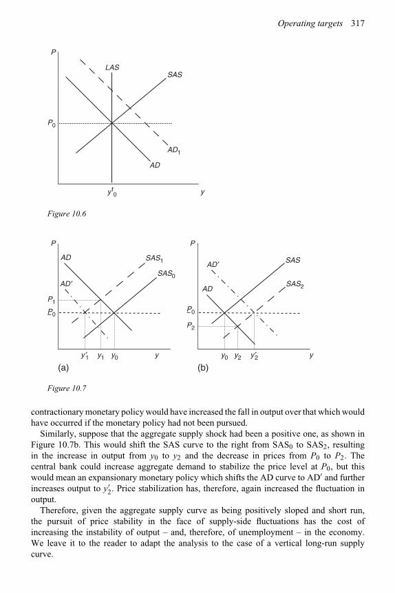
Operating targets 317
P
y f0 y
AD
SAS
P0
AD1
LAS
Figure 10.6
AD SAS1
P1
(a) (b)
P0
SAS0AD ′
P
y ′1 y ′2y1 y2
P
AD ′ SAS
P0
P2
SAS2AD
y0 y0y y
Figure 10.7
contractionary monetary policy would have increased the fall in output over that which wouldhave occurred if the monetary policy had not been pursued.
Similarly, suppose that the aggregate supply shock had been a positive one, as shown inFigure 10.7b. This would shift the SAS curve to the right from SAS0 to SAS2, resultingin the increase in output from y0 to y2 and the decrease in prices from P0 to P2. Thecentral bank could increase aggregate demand to stabilize the price level at P0, but thiswould mean an expansionary monetary policy which shifts the AD curve to AD′ and furtherincreases output to y′
2. Price stabilization has, therefore, again increased the fluctuation inoutput.
Therefore, given the aggregate supply curve as being positively sloped and short run,the pursuit of price stability in the face of supply-side fluctuations has the cost ofincreasing the instability of output – and, therefore, of unemployment – in the economy.We leave it to the reader to adapt the analysis to the case of a vertical long-run supplycurve.
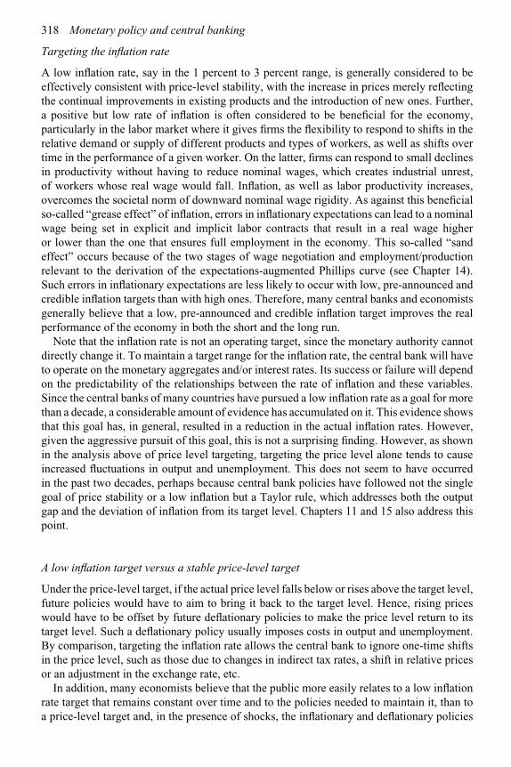
318 Monetary policy and central banking
Targeting the inflation rate
A low inflation rate, say in the 1 percent to 3 percent range, is generally considered to beeffectively consistent with price-level stability, with the increase in prices merely reflectingthe continual improvements in existing products and the introduction of new ones. Further,a positive but low rate of inflation is often considered to be beneficial for the economy,particularly in the labor market where it gives firms the flexibility to respond to shifts in therelative demand or supply of different products and types of workers, as well as shifts overtime in the performance of a given worker. On the latter, firms can respond to small declinesin productivity without having to reduce nominal wages, which creates industrial unrest,of workers whose real wage would fall. Inflation, as well as labor productivity increases,overcomes the societal norm of downward nominal wage rigidity. As against this beneficialso-called “grease effect” of inflation, errors in inflationary expectations can lead to a nominalwage being set in explicit and implicit labor contracts that result in a real wage higheror lower than the one that ensures full employment in the economy. This so-called “sandeffect” occurs because of the two stages of wage negotiation and employment/productionrelevant to the derivation of the expectations-augmented Phillips curve (see Chapter 14).Such errors in inflationary expectations are less likely to occur with low, pre-announced andcredible inflation targets than with high ones. Therefore, many central banks and economistsgenerally believe that a low, pre-announced and credible inflation target improves the realperformance of the economy in both the short and the long run.
Note that the inflation rate is not an operating target, since the monetary authority cannotdirectly change it. To maintain a target range for the inflation rate, the central bank will haveto operate on the monetary aggregates and/or interest rates. Its success or failure will dependon the predictability of the relationships between the rate of inflation and these variables.Since the central banks of many countries have pursued a low inflation rate as a goal for morethan a decade, a considerable amount of evidence has accumulated on it. This evidence showsthat this goal has, in general, resulted in a reduction in the actual inflation rates. However,given the aggressive pursuit of this goal, this is not a surprising finding. However, as shownin the analysis above of price level targeting, targeting the price level alone tends to causeincreased fluctuations in output and unemployment. This does not seem to have occurredin the past two decades, perhaps because central bank policies have followed not the singlegoal of price stability or a low inflation but a Taylor rule, which addresses both the outputgap and the deviation of inflation from its target level. Chapters 11 and 15 also address thispoint.
A low inflation target versus a stable price-level target
Under the price-level target, if the actual price level falls below or rises above the target level,future policies would have to aim to bring it back to the target level. Hence, rising priceswould have to be offset by future deflationary policies to make the price level return to itstarget level. Such a deflationary policy usually imposes costs in output and unemployment.By comparison, targeting the inflation rate allows the central bank to ignore one-time shiftsin the price level, such as those due to changes in indirect tax rates, a shift in relative pricesor an adjustment in the exchange rate, etc.
In addition, many economists believe that the public more easily relates to a low inflationrate target that remains constant over time and to the policies needed to maintain it, than toa price-level target and, in the presence of shocks, the inflationary and deflationary policies

Operating targets 319
that may be needed to maintain the price target. This point becomes important since thetransparency and credibility of policy is important to the public’s expectations on inflationand the impact of monetary policy on the economy. Therefore, central banks have tended toadopt inflation targeting rather than price-level targeting. The popular Taylor rule embodiesthis preference for inflation rather than price-level targeting, with the target inflation rate thatis usually set for developed economies being in the range from 1 percent to 3 percent.
10.6 Determination of the money supply
No matter how the money supply in the economy is defined or measured, several majorparticipants are involved in its determination. They are:
1 The central bank, which, among its other policies, determines the monetary base and thereserve requirements for the commercial banks, and sets its discount rate.
2 The public, which determines its currency holdings relative to its demand deposits.3 The commercial banks, which, for a given required reserve ratio, determine their actual
demand for reserves as against their demand deposit liabilities.11
Some indication of the relative importance of the major contributors to changes in themoney supply would be useful at this point. Phillip Cagan (1965) concluded that, in theUSA, on average over the 18 cycles during 1877 to 1954, the fluctuations in the currencyratio had a relatively large amplitude over the business cycle. They caused about half of thefluctuations in the growth rate of the money stock, while fluctuations in the monetary baseand the reserve ratio accounted for roughly one-quarter each. But, from a secular perspective,by far the major cause of the long-term growth of the money stock was the growth in themonetary base.
Therefore, there is considerable interaction between the behavior of the central bank, thepublic and the commercial banks in the money supply process. This interaction is importantin studying the behavior of the central bank which, as a policy-making body deciding on thetotal amount of money desirable for the economy, must take into account the responses ofthe public and of the commercial banks to its own actions. The behavior of the central bankin the money-supply process becomes a distinctive topic of study, which is pursued later inthis chapter and the next two chapters.
10.6.1 Demand for currency by the public
Fluctuations in the public’s demand for currency relative to its holdings of demand depositsare a significant source of fluctuations in the money supply. The closest substitute – and afairly close one at that – to currency holdings (C) is demand deposits (D), so that most studieson the issue examine the determinants of the ratio C/D, or of the ratio of currency to the totalmoney stock (C/M1), rather than directly the determinants of the demand for currency alone.
The C/D ratio varies considerably, with a procyclical pattern over the business cycle andover the long term. The desired C/D ratio depends upon the individual’s preferences in the
11 These are not the only actors in the money supply process. In particular, in open economies, the balance ofpayments surpluses (deficits) of a country can increase (decrease) its money supply.

320 Monetary policy and central banking
light of the costs and benefits of holding currency relative to demand deposits. Some of thesecosts and benefits are non-monetary and some are monetary.
The non-monetary benefits and costs are related to the non-monetary costs of holding andcarrying currency compared with those of holding demand deposits and carrying checks.They also take into account the general acceptability of coins and notes for making paymentsas against payments by other means. In financially less developed economies, with few bankbranches in the rural areas and with banking usually not open to or economically feasible forlower income groups, even in the urban areas, currency has a clear advantage over checks.However, even in financially advanced economies, cash is almost always accepted for smalleramounts while the use of checks is restricted to payments where the issuer’s credit-worthinesscan be established, or the delivery of goods can be delayed until after the clearance of thecheck through the banks. It is also more convenient to make very small payments in cash thanby writing a check. These aspects of non-monetary costs have changed substantially over timein favor of bank deposits with the expansion of the banking system and the modernizationof its procedures, increasing urbanization, spread of banking machines, common usage ofcredit and debit cards, etc.
As against the greater convenience of currency over bank deposits for transactions, thepossession of a significant amount of currency involves risks of theft and robbery, whichimpose not only its loss but also a risk of injury and trauma to the carrier. The fear of thelatter is often sufficient to deter possession of large amounts of currency in societies wherethis kind of risk is significant. This is so in most countries, with the result that only smallamounts of currency are carried by most individuals at one time or stored in their homes.By comparison, the demand for currency in Japan – a society with a very low rate of theftand robbery – is dominated by its convenience relative to bank deposits. Consequently,few individuals in Japan hold demand deposit accounts, checks are not widely accepted inexchange, even by firms, or given by them for payment of salaries. Many transactions, evenof fairly large amounts, are done in currency.
The monetary costs and benefits of holding currency relative to demand deposits reallyrelate to the net nominal return on the latter since currency does not have an explicit monetaryreturn or service charge, while demand deposits often possess one or both of these. In anycase, even if demand deposits pay interest, there is usually a negative return on them sincebanks incur labor and capital costs in servicing them and must recoup these through a netcharge on them.12
Chapter 4 presented the inventory analysis of the demand for money. This modelis applicable to the demand for currency relative to demand deposits. This was donein Chapter 4. As pointed out there, the problem with an application of this analysisthat takes account only of the monetary cost of using currency versus demand depositsis that it ignores the non-monetary differences in their usage: acceptance in certaintypes of payments, risks of theft and robbery, etc. However, its central conclusion stillholds: the optimal holdings of currency relative to demand deposits will depend on theirrelative costs and the amount of expenditures financed by them. Therefore, assumingboth currency and demand deposits are “normal goods,” an increase in the net cost of
12 One estimate of the average total cost of demand deposits in 1970 was about 2.4 percent of their dollar volume.The cost of time deposits was, by comparison, 0.6 percent if the interest costs were excluded and between5.3 percent and 5.7 percent if the interest costs were included. Approximately 70 percent of the cost associatedwith demand deposits was the cost of processing checks and involved wages, computer time costs, etc.
Operating targets 321
holding demand deposits would increase the demand for currency and hence the C/Dratio.
However, in a time-series context, the major reasons for changes in this ratio have beenthe innovations in shopping, payments and banking practices which have made checkingincreasingly easier and thereby lowered the C/D ratio. In addition, the significant possibilityof theft and robbery – and the consequent risk to the person – with increases over time inmany economies, have kept this ratio quite low or further reduced it. As indicated earlier,Japan, with a low risk from such criminal activities, is an exception to this rule and illustratesthe greater convenience of using currency where a sufficiently wide range of denominationsis made available in bank notes.
For the future, in financially developed economies, smart cards are likely to become a closesubstitute for currency in many transactions that used to be settled in currency since suchcards may prove to be even more convenient than currency and yet not more susceptible totheft. Therefore, the demand for currency as a proportion of total expenditures or of M1 orM2 is likely to continue to decline in the future.
The above arguments imply that the demand function for currency can be written as:
C/D = c(γD,Rh,RD,RT,Y ;payments technology) (4)
where:c = currency-demand deposit ratioγD = charges on demand depositsRh = average yield on the public’s investments in bonds, etc.RD = interest rate on demand depositsRT = interest rate on time depositsY = nominal national income
∂c/∂γD > 0 and ∂c/∂RD < 0 for obvious reasons. We expect ∂c/∂Y > 0, since an increase inY increases transactions that are likely to increase the demand for currency proportionatelymore than for demand deposits. This implies that the currency ratio will increase in theupturns and decrease in the recessions. An increase in the return on both time deposits andbonds is likely to decrease the demand for both currency and demand deposits. Further,currency is needed for small everyday transactions that tend to be inelastic in response tochanges in interest rates, while efficient cash management techniques allow reductions indemand deposits. Hence, the currency ratio will rise with increases in Rh and RT, so that∂c/∂Rh > 0 and ∂c/∂TT > 0. This implies that an increase in the rate of inflation and/orin the nominal interest rate, as usually happens in the upturn of the business cycle, wouldincrease the currency ratio. Conversely, this ratio will fall in a recession. Hence, we expectthe currency ratio to be procyclical (i.e. to rise in upturns and fall in downturns).
As stressed above, the currency ratio also depends upon the security environment and theavailability of alternative modes of payment such as debit and credit cards. The impendinginnovations in creating smart cards that represent electronic purses are likely to reducecurrency demand.
Households not only hold currency and demand deposits but also hold various forms ofsavings deposits, term deposits and their variants. All of these pay interest, and we can specifythe arguments that would lead to the public’s demand function for time deposits or for itsdesired ratio of time to demand deposits. The derivation of these functions is left to thereader.

322 Monetary policy and central banking
10.6.2 Commercial banks: the demand for reserves
Commercial banks hold reserves against their deposits. A part of these reserves is normallyheld in cash (at the tills, in the automatic teller machines or in the bank’s vault) and part isheld in deposits with the central bank. If only a small part of deposits is withdrawn froma bank during a period, the bank does not have to maintain reserves equal to deposits (i.e.follow a 100 percent reserve ratio) but could increase its revenues by lending out a part ormost of its deposits. This leads to fractional reserve banking, where the fraction of depositsheld in reserves may be quite small, as discussed later in this chapter. The reserve ratio isthe ratio of reserves held to deposits.
The central bank often requires the commercial banks to meet a certain minimum ratiocalled the required reserve ratio13 – of their reserves to their deposit liabilities.14 Chapter 11will present the required reserve ratios for several countries. In 1999, this ratio was zero inCanada and the United Kingdom. In the United States, it depended on the amount of depositsand varied between 3 percent and 9 percent for depository institutions.
Banks usually hold reserves in excess of those required to meet the required reserve ratio.Banks also borrow from other banks or the central bank. Reserves held in excess of the sumof required and borrowed reserves are referred to as free reserves – that is, at the bank’sdisposal for use if it so desires.
Free reserve hypothesis
Free reserves for a bank are those it wants to hold in addition to its required reservesand borrowed reserves. Free reserves must be distinguished from excess reserves, whichare actual holdings of cash reserves in excess of the sum of required, borrowed and freereserves. Excess reserves are ones that the bank wants to eliminate either immediately orgradually. The hypothesis for the determination of free reserves is known as the free reservehypothesis.
Required reserves and free reserves depend upon the required reserve ratio or differentialratios imposed by the central bank, discussed in Chapters 11 and 12 on central bank behavior,and upon the total deposits in the bank. The computation of such required reserves is largelymechanical, according to a formula prescribed by the central bank.15
Each bank has to anticipate its deposit liabilities in making its decisions on its reserveholdings. Demand deposits may be withdrawn on demand at any time and individuals’demand deposits in any given bank fluctuate considerably over time as they make depositsand withdrawals. For any given bank over a given period, the totals of new depositsand withdrawals are likely to cancel out to some extent, depending upon its size and thedistribution of its depositors among occupations and industries, between employees andemployers, etc. The degree of uncertainty as to the average levels of deposits in any bank is
13 The next chapter on the central bank discusses required reserve ratios in greater detail. It is now close to zero inmany Western countries, excluding the United States where it is between 3 percent and 10 percent.
14 Some countries, including the United States, have different required ratios for different types of bank liabilitiesor for different financial institutions, depending on their size and nature.
15 The formulae for computing legally required reserves differ between countries, with significant impact on thebehavior of banks toward free reserves and hence toward monetary policy. A significant difference can bewhether the reserves required to be held by a bank are computed as a proportion of its deposits in the currentperiod or some past period, say a few weeks earlier. The former process introduces uncertainty in the amountof required reserves, while the latter does not.
Operating targets 323
thus likely to vary between banks. It is likely to be higher for unit rather than branch banks,small rather than large banks, and banks with a smaller degree of monopoly than those witha greater one. The cancellation process is likely to be still greater for all the banks in theeconomy taken together, so that the overall amounts of demand deposits in the economynormally exhibit a great deal of stability.
For banks, reserves are an asset, in addition to bonds and loans, so that the demand forreserves depends on the returns on the latter. Reserves do not generally earn a monetaryreturn. Their demand should, because of the substitution effect, fall as the rates of return onthe other assets rise, and vice versa.
Under uncertainty, the free reserve hypothesis assumes that banks maximize the expectedutility of their terminal wealth, corresponding to the expected utility maximization by theindividual investor presented in Chapter 5. Therefore, the theory of portfolio selection set outin Chapter 5 can be adapted to explain the bank’s demand for free reserves. Assuming thatthe banks are risk averters, disliking the prospect of ending up with less than the requiredreserves, they would always hold more than the required reserves. Part of these extra reservescould be borrowed, so that the demand for free reserves will depend upon the risks present,the response to risk, the cost of borrowing and the return on other assets in the bank’sportfolio.
A significant element of the risk in falling short of the desired reserves depends on thestructure of the banking system, the size of the bank in question and the diversity of its clientbase. Canadian and British banks tend to be large, with branches all over the country. Theyhave a very diversified client base, so that the daily variance in their deposits is relativelylow. The US banks in the smaller cities and rural areas are often small, have a limited numberof branches and may be dependent on a particular segment of the economy. Consequently,they face higher daily variance in their deposits.
Another significant element of risk in falling short of the desired reserves is related tothe formula specified by the central bank for the minimum reserves that the banks shouldhold against their deposits.16 In the UK, although the reserve requirement is zero (or, rather,non-negative), the banks are expected to meet it on a daily basis. This increases their risk,which to some extent is offset through their ability to borrow reserves in the overnight marketfrom other financial institutions. Canada allows averaging of reserves and deposits over a4 to 5-week period and the United States allows this over 2 weeks, thereby implying less riskfor their banks than for British banks.17
Borrowing by commercial banks from the central bank
Banks borrow reserves from a variety of sources. Banks frequently borrow reserves fromeach other bilaterally and often do so in the context of an organized overnight loan marketsuch as the Federal Funds market in the USA and the Overnight Loan market in Canada. Theycan, depending on regulations, also borrow abroad to supplement their reserves. Borrowingby individual banks from other banks within the system does not change the monetary baseand can therefore be ignored in the determination of the money supply. However, when the
16 Information on these is given in Chapter 11, Table 11.1.17 Another consideration is whether lagged reserve accounting is allowed, i.e. whether the banks can average their
reserves and deposits over a specified past period or have to include the current one. The former involves less risk.
324 Monetary policy and central banking
commercial banks as a whole increase their borrowing from the central bank or from abroad,the monetary base increases and the money supply expands.
In lending to the commercial banks as a whole, the central bank is said to act as the lenderof last resort since the banking system as a whole cannot obtain additional funds from its owninternal borrowing and lending. However, individual commercial banks sometimes treat thecentral bank as their lender of first resort rather than last resort. The terms on which it lendsand the conditions under which its loans are made affect the amounts that the banks wish toborrow from it. In general, borrowing from the central bank can trigger greater oversight bythe central bank into the borrowing bank’s asset management and other practices. Since thisis rarely desired, it acts as a disincentive to borrow.
In the USA, the discount rate – at which the Federal Reserve System lends to its memberbanks – is usually below the three-month Treasury bill rate, so that these banks stand togain by borrowing from the Federal Reserve System. To limit the amounts and frequencyof borrowing, the Federal Reserve Board imposes a variety of formal and informal rules onsuch borrowing. One of the latter is that borrowing from the Federal Reserve System is aprivilege, extended by the Federal Reserve System to its member banks, rather than a rightof the banks. This privilege can be curtailed or circumscribed by conditions if a bank tries touse it indiscriminately.
Canada has experimented with two different methods for setting the bank rate at whichit lends to the chartered banks. Under a fixed bank rate regime adopted from 1956 to 1962and from 1980 to 1994, the bank rate was automatically set each week at 0.25 percenthigher than the average Treasury bill rate that week. Since it was higher than the Treasurybill rate, the chartered banks incurred a loss if they financed their purchases of Treasurybills by borrowing from the Bank of Canada. Such a rate is said to be a “penalty rate”and, by its nature, discourages borrowings. It does not therefore need the support of otherrestrictions on borrowings to the extent that the American discount rate requires. Since1994, the Bank has placed its major focus on setting the overnight loan rate, with anoperating band around it of 50 basis points. This rate is the rate at which the banks andother major participants in the money market make overnight loans to each other. Since1996, the bank rate has been set at the upper limit of the operating range for the overnightloans, so that it is a floating rate and continues to be a penalty rate, irrespective of dailymovements in the market rates. The Bank of Canada influences the Bank Rate by changesin its supply of funds to the overnight market or through its purchases or sales of Treasurybills.
In the United Kingdom, the Bank of England determines daily the rate at which it will lendto the banks. This allows it control over borrowings from it on a daily basis. It also allowsclose control over the interest rates that the banks charge their customers, since these rateshave base rates closely tied to the Bank’s daily rate.
Banks’ demand function for reserves
The free reserve hypothesis, in attempting to explain the demand for free reserves, has totake these differing practices into account and would yield differing demand functions fordifferent countries and periods. However, empirical studies18 have confirmed its implicationthat the earnings on alternative assets influence the amount of reserves held and that the ratio
18 For example, see DeLeeuw (1965), Goldfeld (1966), Frost (1971).

Operating targets 325
of desired reserves to demand deposits cannot be taken as constant for purposes of monetarypolicy.
The preceding arguments imply that the demand function for desired free reserves, FR,can be expressed as:
FR/D = f (R,RBR,RCB) (5)
where:R = average interest rate on banks’ assetsRBR = average return on banks’ reservesRCB = central bank’s discount rate (for loans to the commercial banks)
In (5), ∂f/∂R< 0, ∂f/∂RBR > 0 and ∂f/∂RCB > 0. We have simplified this function by includingaverage interest rates rather than the variety of interest rates that will need to be consideredin practice.
Note that, in (5), R is an average of the nominal returns on Treasury bills, bonds ofdifferent maturities, mortgages and loans to the public, etc. Also note that RBR would be zerofor reserves held in currency and would also be zero if the rest of the reserves were held innon-interest paying deposits with the central bank. Banks will want to increase free reservesif the cost RCB of covering a shortfall in reserves increases and decrease them if the return Rfrom investing their funds rises. Free reserves would also increase if RBR were positive andwere to increase.
10.7 Mechanical theories of the money supply: money supply identities
Mechanical theories of the money supply are so called because they use identities, rather thanbehavioral functions, to calculate the money supply. The money-supply equations resultingfrom such an approach can be easily made more or less complex, depending upon thepurpose of the analysis. We specify below several such equations, starting with the mostelementary one.
An elementary demand deposit equation
Assume that the ratio of reserves held by the banks against demand deposits is given by:
BR = ρD
where:BR = reserves held by banksD = demand deposits in banksρ = reserve ratio
If ρ equals the required reserve ratio, set by the central bank for the banking system, andBR represents the reserves exogenously supplied to it, profit-maximizing banks will createthe amount of deposits given by:
D = (1/ρ)BR (6)
This equation is the elementary deposit creation formula for the creation of deposits bybanks on the basis of the reserves held by them. It suffers from a failure to take note of thebehavior of the banks and the public in the deposit expansion process, so that a more elaborateapproach to the money supply is preferable.

326 Monetary policy and central banking
Common money-supply formulae
Friedman and Schwartz (1963) used a money-supply equation that not only takes account ofthe reserve/deposit ratio of banks but also of the ratio of currency to deposits desired by thepublic. Their ratio is derived simply from the accounting identities:
M = C + D (7)
M0 = BR + C (8)
where:D = demand depositsBR = banks’ reservesC = currency in the hands of the publicM0 = monetary base = BR + C.
The Friedman and Schwartz money-supply formula is derived as follows:
M = M
M0M0 (9)
= C + D
BR + CM0
= 1 + D/C
BR/C + 1M0
= (1 + D/C)(D/BR)
(BR/C + 1)(D/BR)M0
= (1 + D/C)(D/BR)
(D/BR + D/C)M0
Equation (9) separates the basic determinants of the money stock into changes in the monetarybase and changes in the “monetary base multiplier,” defined as (∂M/∂M0), for the monetarybase.19 This multiplier is itself determined by D/BR, the reserve ratio, and C/D, the currencyratio. Of these, the reserve ratio reflects the required reserve ratio and the banks’ demand forfree reserves. The currency ratio reflects the public’s behavior in its demand for currency.Hence, the three determinants of the money stock emphasized by (9) are the monetary base,the currency and the reserve ratios.
Another version of the money-supply formula is:
M = 1(C
M+ BR
D− C
M.BR
D
)M0 (10)
Using this equation, Cagan (1965) examined the contributions of the three elements B, C/Mand BR/D, to M2 over the business cycle and in the long term. He found that the dominant
19 We have designated ∂M/∂M0 the monetary base multiplier, so that it captures the impact of changes in themonetary base on the money supply. Some other authors call it the money multiplier. We have left the latterconcept of multiplier to mean ∂Y /∂M (where Y is national income), as used in Chapters 13 to 15, on themacroeconomy.

Operating targets 327
factor influencing the long-term growth in the money stock was the growth in the monetarybase. Changes in the two ratios contributed little to the secular change in M2. However, forcyclical movements in the money stock the changes in the C/M ratio were the most importantelement, whereas the reserve ratio had only a minor impact and changes in the monetary baseexerted only an irregular influence.
The currency–demand deposit – and hence the currency–money ratio – is influencedstrongly by changes in economic activity and especially by changes in the rate of consumerspending. As we have explained in earlier sections, this ratio varies in the same directionas nominal national income – hence, pro-cyclically – so that a rise in spending in cyclicalupturns increases currency holdings, which lowers the money supply.
The preceding money-supply formula does not differentiate deposits into various typessuch as demand deposits, time and savings deposits, and government deposits nor does itdifferentiate between their reserve requirements. A formula (its derivation is not shown) thatdoes so is:
M =[
1 + c
ρD +ρT t +ρGg + c
]M0 (11)
where t = T/D and g = G/D, T and G represent time/savings deposits and governmentdeposits respectively in commercial banks.
The above formulae are all identities. Which one is used depends upon the rules andregulations about reserve ratios, the availability of statistical data and the further behavioralassumptions that are made. In practice, theories of the money supply go beyond these identitiesand embed the relevant identity in a behavioral theory.
10.8 Behavioral theories of the money supply
A behavioral theory of the money supply process must take into account the behavior of thedifferent participants in this process in order to determine the economic and non-economicdeterminants of the variables being studied. Such a theory studies this behavior in terms ofthe main components of the preceding money supply formulae, such as the currency desiredby the public, the reserves desired by the commercial banks, the amounts borrowed by themand the monetary base which the central bank wishes to provide.
Our earlier discussions on the demand for components of the money supply imply thegeneral form of the money-supply function to be:
M s = M s(RD,RT ,RS ,RL,Rd ,RO,R,Y ,M0) (12)
where:RD = charges on demand depositsRT = interest rate on time depositsRS = short-term interest rateRL = long-term interest rateRd = discount rate (central bank rate for lending to the commercial banks)RO = overnight loan rateRR = required reserve ratio.
As argued in earlier sections, the money supply depends, among other variables, upon thefree reserves desired by the banks and the currency desired by the public. Free reserves depend

328 Monetary policy and central banking
upon RO, Rd , RS and RL since these determine the opportunity cost of holding free reserves.The public’s demand for currency will similarly be a function of RD and RT. It also depends,as argued earlier, on the level of economic activity for which nominal national income Y isa proxy. Finally, the money supply depends upon the monetary base M0.
The monetary base is under the control of the monetary authorities, which can operate itin such a way as to offset the effect of changes in the other variables on the money supply.Alternatively, they may only allow the changes in the other variables to affect the moneysupply in so far as the effect changes the money supply to a desired extent. The monetarybase is, therefore, not necessarily a variable independent of the other explanatory variablesin (12).
Now consider the directions of the effects that are likely to occur in the money-supplyfunction. An increase in the monetary base increases the money supply. An increase innational income increases the currency demand and lowers banks’ reserves and hencedecreases the money supply. An increase in the short-term market interest rate increasesthe profitability of assets which are close substitutes for free reserves and hence decreasesthe demand for free reserves, which increases the money supply. A cut in the discount rate hasa somewhat similar effect. An increase in the yield on time deposits increases their demand bythe public, which lowers the reserves available for demand deposits, so that demand depositsdecrease.
In practice, the estimation of the money-supply function is usually undertaken with asmaller number of variables than those specified in (12). This is partly because of collinearityamong the various interest rates.
Equation (12) specifies the money-supply function and could be applied to the supplyof either M1 or M2 or another monetary aggregate. However, note that the signs of theinterest-rate elasticities could differ among the aggregates. There are three main cases ofdifferences:
1 If the interest rates on demand deposits increase, their demand will increase but thiscould be merely at the expense of time deposits, so that while M1 increases, M2 doesnot do so. Hence, the interest elasticity of demand deposits and M1 with respect to RD
is positive but that of M2 may be positive or zero.2 Since time deposits are excluded from M1, they are part of the opportunity cost of
holding M1. Hence, the elasticity of M1 with respect to the interest rate on time deposits,RT , would be negative. These deposits are, however, part of M2 so that, when theirinterest rate increases, the desired amount of time deposits increases and so does M2.That is, the interest elasticity of M2 with respect to RT is positive.
3 The interest elasticity of M1 would be negative with respect to the return on bonds. Butif the time deposits interest rates rise with this bond rate, the respective interest elasticityof M2 is likely to be zero. However, if the time deposit rates do not increase when thebond rate rises, the public will switch some time deposits to bonds, so that the elasticityof M2 with respect to R would be negative. Therefore, this interest elasticity dependsupon the relationship between RT and R.
Table 10.2 shows the pattern of interest-rate elasticities for M1 and M2. This table alsoincludes the elasticities of M1 and M2 with respect to the return on excess reserves and thecentral bank discount rate on borrowed reserves. Both are negative. The reasons for theseand the other signs shown in Table 10.2 have been explained above.

Operating targets 329
Table 10.2 Money supply elasticities
Interest rate on: M1 M2
Demand deposits + ?Time deposits − +Bonds − ?Excess reserves − −Central bank’s discount rate − −
Interest rate elasticities of the money supply
Empirical studies on money supply are far fewer than on money demand. The following briefreview of the empirical findings on the money supply function confines itself to reporting theelasticities’ estimates for this function.
Rasche (1972) reports the impact and equilibrium elasticities calculated by him for thesupply functions reported by DeLeeuw (1965) for the Brookings model, by Goldfeld (1966)for the Goldfeld model, and for the MPS model developed by the Federal Reserve–MIT–Pennsylvania econometric model project. These studies were for the USA, using data up tothe mid-1960s. Rasche’s calculations of these elasticities are roughly in the ranges reportedin Table 10.3.20
Note that there have been many changes in the United States’ financial markets sincethe 1960s, so that the elasticity ranges reported in Table 10.3 are now mainly useful forpedagogical purposes. These elasticities indicated that the main components of the moneysupply – and the money supply itself – were not exogenous but functions of the interest ratesin the economy. We conclude from Table 10.3 that:
1 Currency demand was negatively related to the time deposit rate, whereas time depositswere positively related.
2 Time deposit holdings were positively related to their own interest rate and negativelyto the Treasury bill rate.
3 Banks increased their borrowing from the Federal Reserve as the Treasury bill rate roseand decreased them as the discount rate increased. Note that the discount rate is the costof such borrowing and the Treasury bill rate represents the return on funds invested bythe banks. Hence an increase in the Treasury bill rate provides an incentive for banks toincrease their loans for a given monetary base, and also to increase their borrowing, giventhe discount rate, from the central bank. Both these factors imply a positive elasticity ofthe money supply with respect to the Treasury bill rate, as shown in Table 10.3.
4 Conversely, while the banks’ free reserves decreased as the Treasury bill increased, theyincreased with the discount rate. The Treasury bill rate represents the amount the bankslose by holding free reserves and is, therefore, their opportunity cost, so that the freereserves fall with the Treasury bill rate. However, these elasticities with respect to thediscount rate are positive since the discount rate is the “return” on free reserves; i.e. ifthey hold adequate free reserves to meet withdrawals, the banks escape having to borrowfrom the central bank at the discount rate.
20 These estimates cover different studies and different periods, and are reported for illustrative purposes only.

330 Monetary policy and central banking
Table 10.3a Interest rate elasticities for the money supply function
Impact b Equilibrium
Currency demandTime deposit rate −0.012 to −0.015 −0.136 to −0.14Treasury bill rate −0.008 to 0.0037 −0.07 to 0.026
Time deposit demandTreasury bill rate −0.038 to −0.15 −0.374 to −1.4Time deposit rate 0.070 to 0.3 0.683 to 2.9
Bank borrowingsTreasury bill rate 0.134 to 0.88 0.50 to 2.625Discount rate −0.186 to −0.98 −0.70 to −2.926
Free reservesTreasury bill rate −2.99 to −3.95 −6.42 to −8.47Discount rate 3.23 to 3.48 6.93 to 7.46
Money supply, excluding time depositsc
Treasury bill rate 0.214 (average over first 6 months)0.267 (average over second 6 months)0.2438 (average over third 6 months)
Money supply, including time depositsd
Treasury bill rate 0.219 (average over first 6 months)0.278 (average over second 6 months)0.258 (average over third 6 months)
a Compiled from Rasche (1972), various tables.b The impact elasticity is over the first quarter following a change in the interest rate.c From Rasche (1972), Table 5.d From Rasche (1972), Table 5.
These reported elasticities are consistent with the analysis presented earlier in thischapter. Even though there have been numerous innovations in the financial markets sincethe 1960s, so that the magnitudes of the actual elasticities are likely to have changed,there is no reason to expect that the signs of elasticities have altered from those reportedabove.
Lags in the money-supply function
The main findings on this show that:
1 The impact elasticities are significantly lower than the equilibrium ones, indicating thatthe adjustments take longer than one quarter.
2 The money supply had positive interest elasticities each month through the first 18 monthsfor which the elasticities were reported.
These findings show that the financial sector did not adjust the money supply to its fullequilibrium level within one quarter. In fact, the second finding points out that the moneysupply continues to change even after six quarters. This finding has been confirmed by manystudies, so that the existence of lags in the response of the money supply to interest-ratechanges can be taken as being well established.

Operating targets 331
10.9 Cointegration and error-correction models of the money supply
There are few cointegration studies on the money supply function and its major components.We draw the following findings from Baghestani and Mott (1997) to illustrate the nature ofempirical findings on money supply and the problems with estimating this function whenmonetary policy shifts.
Baghestani and Mott performed cointegration tests on USA monthly data for three periods,1971:04 to 1979:09, 1979:10 to 1982:09 and 1983:01 to 1990:06, using the Engle–Grangertechniques. Their variables were log of M1, log of the monetary base (B) and an interestrate variable (R). The last was measured by the three-month commercial paper rate for thefirst two periods and by the differential between this rate and the deposit rate paid on SuperNOWs (Negotiable Orders of Withdrawal at banks) introduced in January 1983. Further, thediscount rate was used as a deterministic trend variable, since it is constant over long periods.The data for the three periods was separated since the Federal Reserve changed its operatingprocedures between these periods.
Baghestani and Mott could not reject the null hypothesis of no cointegration among thedesignated variables for 1971:04 to 1979:09. Further, for 1979:10 to 1982:09, while M0and R possessed a unit root, M1 did not, so the cointegration technique was not applied forthis period. The only period which satisfied the requirement for cointegration and yielded acointegration vector was 1983:01 to 1990:06. The error-correction model was also estimatedfor this period. The cointegration between the variables broke down when the period wasextended beyond 1990:06. These results have to be treated with great caution. As indicatedin Chapter 9 on money-demand estimation, cointegration is meant to reveal the long-runrelationships and, for reliable results, requires data over a long period rather than morefrequent observations, as in monthly data, over a few years. The three periods used byBaghestani and Mott were each less than a decade.
For 1983:01 to 1990:06, Baghestani and Mott concluded from their cointegration–ECMresults that the economy’s adjustments to the long-run relationship occurred through changesin the money supply and the interest rate, rather than in the monetary base. Comparingtheir findings across their three periods, we see that changes in the central bank policyregime, such as targeting monetary aggregates or interest rates, are extremely important indetermining the money supply function in terms of both its coefficients and whether thereeven exists a long-run relationship. Further, even regulatory changes such as permitting,after 1980, the payment of interest on checkable deposits can shift the money-supplyfunction.
10.10 Monetary base and interest rates as alternative policyinstruments
The central bank may use either the monetary base or the interest rate as a way of controllingaggregate demand in the economy, or may have to use both. Under certainty and knownmoney supply and demand functions, it needs to use only one of them since the use of eitherof them indirectly amounts to use of the other. To see this correspondence, assume that themoney supply function is given by:
M = M0[C
M+ BR
D− C
M· BR
D
] (13)

332 Monetary policy and central banking
where the meanings of the symbols are as explained earlier. This money supply function canbe written simply as:
M = αM0, (14)
where:
α = 1[C
M+ BR
D− C
M.BR
D
]
where α is the “monetary base (to money supply) multiplier” ∂M/∂M0, though some authorscall it the “money multiplier,” a term that we have more appropriately reserved for ∂Y/∂M ,where Y is nominal national income.
Let the general form of the money demand function be:
md = md(y,R) (15)
where R is the nominal interest rate and y can be the pre-specified actual or desired level ofoutput. In money market equilibrium, we have:
α.M0 = P.md(y,R) (16)
Under certainty, given the policy targets for P at P∗ and y at y∗, (16) can be solved for therelationship between M0 and R, so that the central bank can achieve its objectives by settingthe monetary base M0 at M0∗ and letting the economy determine R, or by setting R at R∗ andletting the economy determine the money supply needed to support R∗. It does not have topursue a policy of setting both M0 and R.
Making the choice between the interest rate and the monetary base as operatingtargets in a stochastic context
In developed economies, adequate reasons for the choice between M0 and R as the optimalmonetary policy instrument arise only if there is uncertainty and unpredictability of the moneysupply and/or demand functions.21 In this scenario, the policy maker may not know whichpolicy instrument would more predictably deliver the target values y∗ and P∗. In general, inthe absence of any sure information, the theory of policy under uncertainty implies that therisk-averting policy maker should diversify by using both policy instruments. However, asPoole’s analysis presented earlier in this chapter (and in Chapter 13) shows, if the main shocksto aggregate demand originate from shifts in the commodity sector, then the money supplyis, in general, the preferable monetary policy instrument. But, if the main shocks to aggregatedemand originate in the monetary sector, the interest rate is, in general, the preferable one(Poole, 1970). The next chapter examines this issue in greater detail.
21 Note that even if the deterministic elements of the two functions are known, there will also be a stochasticcomponent which will be unpredictable.

Operating targets 333
Another reason for the choice between the two instruments can arise because of the natureof the economy. Underdeveloped financial economies usually do not have well-developedbond markets, which prevents the central bank from effectively using open-market operations.However, there may be other ways of changing the monetary base, such as by feedingincreases in the money supply to the government to finance its deficits. In addition, changesin the reserve requirements can be used to change the supply for a given monetary base. Sucheconomies also have fragmented financial markets, along with a large informal financialsector, so that there need not be a close relationship between the interest rate set by thecentral bank and that charged in the various private financial markets. Further, much of theinvestment in these economies may not be sensitive to market interest rates. Therefore, onthe whole for such economies, it is likely that changes in the money supply will be moreeffective, though not perfectly so, in manipulating aggregate demand than will changes inthe interest rate. However, given the imperfections of both policy instruments in controllingaggregate demand, demand management would work better if the central bank were to useboth instruments.
Conclusions
This chapter has examined the implications of adopting different operational targets formonetary policy. For most central banks, the direct target is no longer a reserve aggregate suchas borrowed or non-borrowed reserves, the monetary base or a monetary aggregate (M1, M2,M3 or M4), since these proved to have an unstable relationship with nominal GDP in the1980s and 1990s. The main reason for this instability has been financial innovation leadingto changes in the velocity of circulation, new monetary assets and increased substitutabilitybetween demand deposits and other financial assets.
Even though the role of the money supply has been downgraded in recent years, it remainscritical to the economy’s economic performance. The theory of money supply for any giveneconomy therefore, has to start with the knowledge of whether or not its central bankexogenously determines the money supply, thereby canceling out any undesired changesin it induced by other factors in the economy. If it does so, the final determinant of the moneysupply is central bank behavior. However, if it allows other factors some role in changing themoney supply, a wider analysis of the money supply becomes applicable and the behaviorof the public and of financial institutions also needs to be studied.
The theories of money supply can be specified as either mechanical or behavioral.In practice, most empirical studies combine both approaches in deriving their estimatingequations. These studies show that, over time, changes in the monetary base are the mainelement of changes in the money supply. However, over the business cycle, changes in thecurrency and the reserve ratios also play a very significant role, with the result that theirdeterminants also need to be incorporated into the estimating equations. These determinantsinclude a variety of interest rates in the economy, as well as national income. The estimatedmoney supply functions, especially for M1, usually show negative elasticities with respectto the central bank discount rate and positive elasticities with respect to the Treasurybill rate.
The application of cointegration techniques to the money supply and its determinants isnot as common as for the money demand function. Cointegration requires long runs of datafor reliable results. Since the money supply depends critically upon central bank behavior,periodic changes in the central bank’s targets and money supply rules make it difficult

334 Monetary policy and central banking
to collect sufficient data for reliable cointegration results on the money supply function.However, the reported empirical studies on this function do usually yield signs consistentwith the signs of the interest-rate elasticities implied by the theory.
Summary of critical conclusions
❖ Successful interest-rate targeting, in comparison with monetary targeting, increases theimpact on aggregate demand of investment, net exports, fiscal deficits and other disturbancesin the commodity markets while eliminating the impact of shocks emanating from thefinancial sectors.
❖ Monetary targeting eliminates the impact of fluctuations in the money supply induced bythe private sector and moderates the impact of fluctuations emanating from the commoditymarket.
❖ The public and the banks affect the money supply by changes in the currency ratio and freereserves, so that the central bank must be able to predict these ratios if it is to offset themand control the money supply in the economy.
❖ Empirical studies support a behavioral approach to the money supply and indicate that themoney supply depends on the interest rates in the economy. The estimated money supplyfunctions are sensitive to monetary policy and target regimes.
Review and discussion questions
1. Discuss, using diagrams, the following statement: if the money demand function has ahigh interest inelasticity, the case for a monetary aggregate as against an interest rate asthe central bank’s operating target is strengthened, especially in an economy subject tostochastic shocks.
2. How do central banks manage interest rates in your country and one other country ofyour choice? What consequences for output fluctuations can the central bank expectfrom targeting interest rates?
3. The monetary sector has become increasingly unstable in recent years. Does this meanthat the monetary authority should stay with the pursuit of interest-rate targets and leavethe money supply alone?
4. Note that recessions seem to be caused by either reductions in aggregate demand or inaggregate supply, or by the two acting in concert. What targets should the central bankadopt? Would the optimal choice of the target be the same for reductions in aggregatesupply as for reductions in aggregate demand?
5. “Macroeconomic models assume that the money supply is exogenously specified by thecentral bank. If this is so, there is no purpose to the specification and estimation of moneysupply functions.” Discuss this statement. How would you verify its validity?
6. What happens to the monetary base and the money supply if the government finances afiscal deficit by:
(a) selling bonds to the public;(b) selling bonds to the commercial banks;(c) selling bonds to the central bank;(d) selling bonds to foreigners.

Operating targets 335
If any of these changes the money supply, what policies should the central bank adoptto offset these changes?
7. What happens to the monetary base and the money supply if:
(a) the central bank lowers the discount rate;(b) the central bank lowers the discount rate and also sells bonds to the public;(c) the central bank forbids overnight loans and eliminates the overnight loan market.
8. Show what happens to the money supply if:
(a) the economy enters a boom and interest rates rise;(b) the underground economy with illegal holdings of currency is eliminated;(c) firms give a significant discount for payment in cash rather than credit cards;(d) credit cards are replaced totally by debit cards;(e) both credit and debit cards are replaced by smart cards.
9. Does the central bank have tight control over the money supply? What are the factorsthat weaken the link between the central bank policies and changes in the moneysupply?
10. Would a high (in the limit, 100 percent) reserve requirement imposed on banks strengthencentral bank control over the money supply? If so, why do central banks never imposevery high reserve requirements?
11. Discuss what will happen to the monetary base and the money supply if the central bankstarts paying interest, say at the Treasury bill rate, on commercial bank deposits withit. If it does so, would the interest elasticity of money supply be higher or lower than itwould be under a regime where interest was not paid on such deposits?
12. Specify the behavioral money supply function that captures the behavior of the centralbank, the public and the banks in the money supply process. Discuss and compare itslikely interest-rate elasticities for M1 and M2.
13. Let BR (bank reserves) be:
BR = kD + ER
Assume:
ER = f (R,Rd)D ∂ER/∂R < 0,∂ER/∂Rd > 0
where ER is excess reserves, R is the market interest rate, Rd is the central bank’s discountrate and the meanings of the other symbols are as specified in the chapter. Also, let:
C/D = c
Derive the money supply M s(= C +D) as a function of k , c, R, Rd and M0 (the monetarybase), and specify the signs of its partial derivatives.
14. Given the information in the preceding question,
(i) If k = 0.05, ER = 0.01D, c = 0.2, C + D = 0.03 y, derive M0 as a function of y.Also, derive C, D and BR as functions of y.
(ii) Suppose financial innovations shift the demand for currency such that c becomes 0.1.Derive the monetary base as a function of y. How could the central bank offset theimpact of this shift in currency demand on the money supply? Discuss.

336 Monetary policy and central banking
15. Specify a money supply function in terms of the currency and reserve ratios and themonetary base. Let the real money demand function be:
md = md(y,R) = myy − mRR + FW0 ∂md/∂y > 0,∂md/∂R < 0,∂md/∂W > 0
where FW 0 is financial wealth.
(i) Given the need for money market equilibrium, show how the central bank can useM0 as its monetary policy instrument for changing Y (= Py).
(ii) Given the need for money market equilibrium, show how the central bank can use(a) R, (b) Rd , as its policy instrument for changing Y .
(iii) Given the need for money market equilibrium, how would an increase in the pricesof stocks, which increases FW, change M0, R and Rd?
16. How would you formulate your money supply function for estimation in an empiricalstudy? What would be your definition of the money supply variable? What would be thearguments of your function? Justify each one. Comment on the a priori relationships thatyou would expect between your independent variables and the money supply. Compareyour supply function with some others estimated in the literature, and comment on thedifferences.
17. For a selected country and using quarterly data, specify and estimate the money supplyfunction. Among your independent variables, include at least two different interest rates,one being the discount/Bank rate and the other a market-determined short-term rate.Check and correct for shifts in the money supply function during the period of yourstudy. Carry out your estimations using the following techniques:
(a) least-squares estimation, with a first-order PAM;(b) cointegration with an error-correction model.
Discuss your choice of the functional form of the money supply function and yourchoice of the variables and econometric techniques used, as well as the data andeconometric problems you encountered.
Discuss your results, their plausibility and consistency with the theory, and theirrobustness. Can you explain the estimated shifts in your function by reference to changesin the policies of the central bank?
18. What are the reasons for requiring the use of cointegration techniques in estimating themoney supply? What would be the disadvantages of using ordinary least squares forsuch estimation? If you use both and obtain different estimates, which would you relyon and why?
19. Are there, in general, any problems with the application of cointegration techniques tomoney supply functions, or with the interpretation of estimates? Can these estimates berelied upon? Discuss.
References
Baghestani, H., and Mott, T. “A cointegration analysis of the U.S. money supply process.” Journal ofMacroeconomics, 19, 1997, pp. 269–83.
Cagan, P. Determinants and Effects of Changes in the Stock of Money, 1875–1960. New York: ColumbiaUniversity Press, 1965.
De Leeuw, F. “A model of financial behaviour.” In J.S. Duesenberry et al., eds, The Brookings QuarterlyEconometric Model of the United States. Chicago: Rand McNally, 1965, Ch. 13.

Operating targets 337
Friedman, M., and Schwartz, A.J. A Monetary History of the United States, 1867–1960. Princeton, NJ:National Bureau of Economic Research, 1963.
Frost, P.A. “Banks’ demand for excess reserves.” Journal of Political Economy, 79, 1971, pp. 805–25.Goldfeld, S.M. Commercial Bank Behaviour and Economic Activity. Amsterdam: North-Holland, 1966.Poole, W. “Optimal choice of monetary policy instruments in a simple stochastic macro model.”
Quarterly Journal of Economics, 84, 1970, pp. 197–216.Rasche, R.H. “A review of empirical studies of the money supply mechanism.” The Federal Reserve
Bank of St Louis Review, 54, 1972, pp. 11–19.
11 The central bankGoals, targets and instruments
This chapter focuses on the institutional and historical aspects of the goals, instruments andtargets of monetary policy as they have been pursued by the central banks of the United States,Britain and Canada – with some material on the newly created European System of CentralBanks. This material is intended to widen the discussion beyond the particularities of any onecountry and to provide some indication of the similarities and varieties of central bank practicesin the pursuit of monetary policy.
Key concepts introduced in this chapter
♦ Central banks’ mandates♦ The potential multiplicity of goals of central banks♦ Open market operations♦ Required reserves♦ Discount/bank rate♦ Credit controls♦ Moral suasion♦ Selective controls♦ Overnight loan interest rate♦ Federal Funds rate♦ Administered interest rates♦ Currency boards♦ The competitive supply of money
Economic theory has long recognized the impact of monetary policy upon most of theimportant macroeconomic variables such as output, employment, growth and prices.1
Therefore, in most countries, the control of the money supply and the manipulation ofinterest rates, in so far as these are possible, is entrusted to the central bank rather thanleft to market forces.2 This chapter looks at the basic practical and institutional aspectsof the goals and targets of central bank policies, and related issues such as the regulation of
1 See Chapter 2 for the economic heritage on this, and Chapters 13 to 16 for a modern treatment.2 However, there are economists, belonging to the new monetary school, who espouse competitive issue of money
by private institutions. Such issue of money, even bank notes, by private firms was common in most countriesuntil the twentieth century.

The central bank: goals 339
financial intermediaries. Institutional arrangements and practices are specified for the FederalReserve System of the United States, the Bank of Canada, the monetary arrangements inBritain and the European System of Central Banks, which is the federated central bank forthe European Union. The intention in presenting this material on several countries is to showthe common elements as well as the diversity of monetary arrangements among a group ofcountries.
Section 11.1 examines the historically multiple goals of central banks and Section 11.2investigates their evolution to the present goals, which are price and stability, with outputat full employment. Section 11.3 reviews the instruments by which central banks conductmonetary policy. Sections 11.4 and 11.5 focus on the issues of competition and regulationof the financial sector and interest rates. Section 11.6 provides information on the monetaryconditions index, which is used as a guide to monetary policy. Section 11.7 relates theevolution of goals of the central bank to the Taylor rule. Section 11.8 appends a briefdiscussion of currency boards, which represent an alternative institutional arrangement tocentral banks.
11.1 Historic goals of central banks
The central banks of different countries usually have their own distinctive and somewhatdifferent sets of goals in their mandates from their respective legislative authorities. However,as we shall see in this section, there is also a high degree of similarity in the goals, broadlydefined, among them. Further, the mandate assigned to a given central bank is normally broadenough to allow it a great deal of latitude in the goals it does choose to pursue in practice.We illustrate the types of goals usually assigned to central banks by looking at those for theUSA, Canada and the UK.
Original mandate of the Federal Reserve System in the USA
The Federal Reserve System, referred to as the Fed, is the central bank of the United States.It was set up in 1913 and has a Board of Governors3 with a Chairman at its head. Its monetarypolicy is set by the Federal Open Market Committee (FOMC), which consists of the Boardof Governors and five of the presidents of the twelve Federal Reserve Banks. FOMC sets theFederal Funds rate, which is the rate at which commercial banks trade reserves with eachother through overnight loans.
A publication of the Federal Reserve System of the USA listed the broad objectives of thesystem as:
To help counteract inflationary and deflationary movements, and to share in creatingconditions favorable to sustained high employment, stable values, growth of the country,and a rising level of consumption.
It might have also added the additional objective of promoting a favorable balance ofpayments position. The list of economic goals in the mandates assigned until the 1980sto most central banks was very similar to the above multiplicity of goals.
3 The seven governors are appointed for 14-year terms, which contributes to their independence from the governmentof the day. The Federal Reserve System is made up of 12 regional Federal Reserve Banks, located in differentparts of the USA.

340 Monetary policy and central banking
Original mandate of the Bank of Canada
The Bank of Canada was set up in 1934. It has a board of directors and a Governor, whodecide on monetary policy. The preamble to the Bank Act of 1934, setting up the Bank ofCanada, stated that the mandate of the Bank was to be:
To regulate credit and currency in the best interests of the economic life of the nation, tocontrol and protect the external value of the national monetary unit and to mitigate by itsinfluence fluctuations in the general level of production, trade, prices and employment,so far as may be possible within the scope of monetary action, and generally to promotethe economic and financial welfare of Canada.
This preamble required the Bank of Canada to use monetary policy to achieve multiplegoals. There was an implicit assumption behind the preamble that it was within the Bank’spower to affect not only the rate of inflation and the exchange rate, but also the real – and notmerely the nominal – variables of output and employment. On the latter, the assumption wasthat the Bank could affect the short-run values of these real variables and thereby influencetheir fluctuations.
Evolution of the Bank of England and the goals of monetary policy in the UK
The Bank of England was founded as a private commercial bank in 1694.4 Although aprivately owned bank until 1946, it acted from the very beginning as the banker for theBritish government, under a business arrangement entered into in exchange for large loansmade by the Bank to the British government through its purchase of government bonds. It wasgiven the monopoly of (future) note issue in 1844, when it also withdrew from commercialbanking. Its notes were made legal tender and convertible into gold at a fixed exchange rate.It evolved into a central bank through custom and practice in the eighteenth and nineteenthcenturies, only gradually increasing its responsibility for maintaining orderly conditions inthe money markets and influencing the policies and practices of the other commercial banks.
Given its origin as a private bank and its gradual evolution in practice into a central bank,there was no explicit legislated mandate for the Bank of England to pursue monetary policy inorder to achieve specific national macroeconomic goals, even though it interacted closely withthe government. Its primary goals through the eighteenth and nineteenth centuries seemedto be mainly related to maximizing its own profits and preserving its own solvency. Thiswas consistent with the tenor of traditional classical ideas, which did not possess a theoryof monetary policy for manipulating the economy and did not espouse an active monetarypolicy for stabilizing it.
Since the nationalization of the Bank of England in 1946, the relationship between theBank of England and the government – represented by the Chancellor of the Exchequer, whois the government minister in charge of the Treasury – has gone through two distinct phases.From 1946 to 1997 the government had statutory power over not only the goals but alsothe use of instruments of monetary policy, though the day-to-day operations and the normalbusiness were left to the Bank. The Bank made recommendations to the Chancellor, who hadthe final decision on the goals being pursued. The Bank implemented the policies defined by
4 Its ownership was nationalized in 1946.
The central bank: goals 341
the Chancellor, though with some discretion over the timing of implementation of decisions.Consequently, the goals pursued for the economy through monetary policy were ultimatelythose of the government and depended upon the preferences of the party in power. In 1997,however, the Bank was given operational independence in implementing monetary policy,but the power to set the ultimate goals of monetary policy was retained by the Chancellorand, therefore, by the government.
Given this division of powers in Britain between the Bank of England and the government,it is appropriate to use the term “monetary authority” to encompass both of them in their jointroles of setting the goals and pursuing the implementation of monetary policy. By comparison,in the United States and Canada, the monetary authority will simply be their respective centralbanks.
In practice, the historic goals of the monetary authority in the UK were very similar to thoseof the central banks in the USA and Canada. From 1946 to the early 1980s, these policieswere based on a wide set of goals, including lower unemployment, higher growth, lowerinflation and the maintenance of the exchange rate, under the notion that it was possible toachieve several goals or at least trade off among them through monetary policy.
Mandate of the European Central Bank
The gradual bonding of the European countries during the postwar years and their eventualmerger into the European Union in the 1990s resulted in their monetary unification in thatdecade. The central element of this unification is the European System of Central Banks(ESCB), established under the Maastricht Treaty of 1992. The ESCB consists of the EuropeanCentral Bank (ECB), based in Frankfurt, and the national central banks of the membercountries, and is federalist in structure. The central decision-making body on monetary policyis the ECB’s Governing Council, composed of the national central bank governors5 andthe Executive Board6 of the ECB. The Executive Board, besides running the day-to-dayoperations of the ECB, carries out the decisions of the Governing Council and coordinatestheir implementation by the national central banks in their respective countries.
Since the European Central Bank was set up recently, its mandate reflects current thinkingon monetary policy. Its charter states that the “primary objective” of the European System ofCentral Banks (ESCB) should be to “maintain price stability.” The charter also establishes thecomplete independence of the ECB and the national banks from their various governments,so that they are protected from having to take instructions from governments.
The ESCB uses changes in interest rates as the main operational tool of monetary policy,but continues to attach importance to the evolution of monetary aggregates, especially M3,as a guide for its policies.
Additional mandates of the central banks in the LDCs
Most less-developed countries are unable to raise the revenue internally to cover their fiscal,with the result that they continually incur large fiscal deficits. Some of these tend to be
5 Each of them is appointed for a minimum term of five years and cannot be dismissed by their respectivegovernments.
6 The Executive Board has a President and five members, appointed by the European Council for eight year,non-renewable, terms.

342 Monetary policy and central banking
covered by foreign borrowing by the government, but very often there is still a remainderthat needs to be financed. While such deficits in the richer and financially developed nationsare normally covered by the government borrowing directly from the public through theissue of short- and long-term bonds, the financial markets in the LDCs are too thin tosupport much governmental borrowing. Given this constraint, many governments in theLDCs rely upon the central bank to directly finance the remaining deficit through increasesin the monetary base, or to do so indirectly by the sale of government bonds to thecentral bank.
Hence, while the LDCs have broadly similar mandates for their central banks as in theindustrialized countries, an additional one in practice is that of financing the fiscal deficit.The justification sometimes given for this is that of national interest. In some cases, thedeficit is related to massive development programs, so that the central bank’s financingof the deficit is further claimed to be a contribution to national economic development.However, such a practice makes monetary policy subservient to fiscal policy, and hasimplications for the independence of the central bank from the government and for its controlof inflation.
11.2 Evolution of the goals of central banks
Revision in economic theory and the implied limitation on goals
The 1970s were a period of expansionary monetary policy but were accompanied bystagflation in Western economies. This combination produced a period of increasing doubtsabout the relevance and validity of Keynesian policy prescriptions, which, in turn, proved tobe a fertile ground for the emergence and acceptance of resurgent neoclassical theories. Anearly element in this resurgence was in the revision of the Phillips curve to the expectations-augmented Phillips curve (see Chapter 14), often associated with Milton Friedman. Friedman(1977) argued that there was a short-run trade-off only between the unemployment rateand the deviation of the inflation rate from its expected level. But there was no long-run trade-off between unemployment and inflation. Hence, monetary policy had a verylimited ability to change the unemployment rate. The 1970s also saw the introduction ofthe hypothesis of rational expectations. Lucas, Barro, Sargent and Wallace, Kydland andPrescott and others in the 1970s and 1980s laid the foundations of the modern classicalmodel with rational expectations and the neutrality of systematic monetary policy as its coreelements (see Chapters 14 and 16). Only random monetary policy could affect short-runoutput but such a policy would be meaningless. Systematic increases in money supply, underconditions of symmetric information between the monetary authority and the public, wouldbe anticipated but could not bring about the deviation of employment from its equilibriumlevel.
In the 1980s, the impact of this theoretical revision in the scope of monetary policy was topersuade the central banks of many countries to abandon the multiplicity of goals in favor of aheavy and sometimes sole focus on controlling the rate of inflation. While formal legislativerevision of the traditional mandates of the central banks was rare, in practice there was aconsiderable reduction in the emphasis on using monetary policy to change unemploymentand output. The primary goal of monetary policy became a low inflation rate and the resultingpolicy became one of “inflation targeting.” The success of the inflation targeting policy sincethe 1980s in reducing inflation on a long-term basis, accompanied by increasing output andemployment, has led to a general adoption of inflation targeting as the primary objective

The central bank: goals 343
of central banks in many countries. As of 2002, inflation targeting had been adopted in22 countries, including Canada and New Zealand (which had started this policy), the UK andthe USA. However, the objective of ensuring full employment has not disappeared, sinceboth inflation targeting and output targeting are components of the popular Taylor rule (seeChapters 12 and 13) for setting interest rates.
Evolution of the goals of the monetary authorities in Britain
As discussed earlier, the British monetary authority from 1946 to the early 1980s possesseda multiplicity of goals. While the goal of price stability had been one of those goals and hadreceived increasing emphasis by the end of the 1980s, the sole focus on it was made explicitin 1992 when the Chancellor of the Exchequer announced the adoption of explicit inflationtargets (1 percent to 4 percent) aimed at achieving long-term price stability. This adoptionof an explicit target for the inflation rate represented an explicit abandonment of other goalssuch as those on unemployment and output growth, exchange rate stability and business cyclestabilization.
The Chancellor and the Bank periodically set the inflation target. The official inflationtarget was changed in 1995 by the Chancellor, with the agreement of the Bank of England,to a point target of 2.5 percent. It is currently (2008) at 2 percent, along with a set range foracceptable fluctuations in inflation. The primary objective of monetary policy in Britain isnow explicitly that of price stability and only secondarily growth and employment objectives.The implementation of monetary policy, such as the setting of the Bank rate, since 1997 hasbeen left to the Bank and its Monetary Policy Committee. Goodhart (1989, 1995) providesan excellent statement of central banking from a British perspective.
Evolution of the goals of the Bank of Canada
In the late 1980s, the Governor of the Bank of Canada publicly argued that the mandateof the Bank should be changed to focus only on price stability as its mandated goal.The proposal was considered in 1992 by a parliamentary committee, which decided toleave the Bank’s mandate as it had been specified in the Bank of Canada Act of 1934,i.e. with a multiplicity of goals. However, several successive Governors of the Bank inthe late 1980s and the 1990s have advocated and in practice consistently focused solelyor mainly on the goal of price stability or a low inflation rate. Since 1991 the Bankhas announced explicit targets, with an average of 2 percent and a range of 1 percentto 3 percent, for the core inflation rate. These targets have been set jointly by the Bankof Canada and the Government of Canada.7 Movements in other variables such as theexchange rate and asset prices are taken into account to the extent that they affect therate of current or future inflation. In the case of a deviation of the actual inflation fromthe 2 percent target, the Bank normally aims at bringing inflation back to its targetover a six to eight-quarter period. The Bank uses a Monetary Conditions Index (MCI)(explained later in this chapter), which is a weighted sum of the interest rates and theexchange rate, as an operational guide. It uses the overnight loan rate for reserves asits operational target, with a range of 50 basis points. The Bank Rate – on its loans to
7 In Canada, the inflation target is set every five years. In 2006, the government and the Bank of Canada renewedthe inflation target of 2 percent, with a range of 1 percent to 3 percent.

344 Monetary policy and central banking
banks and some other financial institutions – is now set at the upper limit of the targetrange.
New Zealand’s experiment on the goal of price stability
New Zealand was the first country to explicitly adopt inflation targeting. After an extendedperiod of double-digit inflation for much of the late 1970s and 1980s, as well as unsatisfactorygrowth, major legislative changes were made to the country’s monetary arrangements in themid-1980s and in 1990. Among these was the grant of a limited degree of independence tothe central bank, the Reserve Bank of New Zealand, to formulate and implement monetarypolicy so as to maintain price stability. However, on the formulation of the goals of monetarypolicy, it required the Minister of Finance and the Governor of the central bank to jointlyestablish the specific inflation target, its range and the inflation index to be used for thetarget. This information is communicated to the public. These agreements are renegotiated atcertain intervals and leave a measure of flexibility in meeting changing economic conditions.The target ranges for inflation were 3–5 percent from 1990 to 1992, 0–2 percent from1992 to 1996 and 0–3 percent since 1996. Permissible breaches of the established targetare allowed in special circumstances, such as natural disasters, changes in indirect taxesand significant relative price shocks. The Reserve Bank of New Zealand currently uses theMonetary Conditions Index, a concept pioneered by the Bank of Canada. This index is aweighted sum of an interest rate measure and the exchange rate, and is used as a guide formonetary policy.
The New Zealand pattern is similar to that in Britain, and to some extent that in Canada.Its central bank has operational independence but not total independence over the ultimategoals of monetary policy. The goal is limited to that of price stability by legislation, and thelegislation requires that the target range be set jointly with the government.8
Recent pattern of the goals of monetary policy in the United States
The pursuit of goals by the Federal Reserve System changed in the 1980s and 1990s in amanner similar to that in the other countries discussed above, from the pursuit of multiplegoals during the pre-1980 period to that of price stability. One difference between the Fedand the British and Canadian monetary authorities is that the Fed does not set explicit targetsfor the rate of inflation, though its pursuit of a low rate of inflation consistent with pricestability is not in doubt and is often asserted by the chairman of the Board of Governors ofthe Fed. Taylor (1993) argued that the Fed had effectively moved to a monetary policy rule(see the Taylor rule later in this chapter and in Chapters 12 and 13) incorporating inflationtargeting.
The Fed is more genuinely independent of the United States’ President and governmentthan are the Bank of England or the Bank of New Zealand of their governments, in termsof both the formulation of its goals and their pursuit through its monetary policies. There isno question of the government issuing formal instructions to the Fed on the further pursuitof monetary goals or instruments, of requiring it to write open letters to the governmentexplaining its actions, or of penalties being imposed for a failure to achieve price stability.
8 What is distinctive about the New Zealand case is that the Governor of the Bank can be held responsible forfailure to achieve the announced targets, and sanctions may be imposed for such failure.

The central bank: goals 345
11.3 Instruments of monetary policy
The central bank pursues its monetary policy through the use of one or more of theinstruments at its disposal. The mix of the instruments used depends upon the structureof the economy, especially the financial system, and tends to depend on the stage ofdevelopment of the bond and stock markets. The most common instrument among developedcountries is often the change in interest rates, which is usually supported by open marketoperations.
11.3.1 Open market operations
Open market operations9 are the purchase (or sale) by the central bank of securities infinancial markets, resulting in corresponding increases (decreases) in the monetary base.10
Countries with well-developed financial markets and extensive amounts of public debt tradedin the financial markets usually rely on such operations, which, along with the shiftingof government deposits between the central bank and the commercial banks, are the mostimportant tool for changing the money supply. However, this does not hold a correspondingposition among the countries around the world since its prominent position requires certainpreconditions to be met. The most important of these are:
1 The financial structure of the economy should be well developed, with most of theborrowing and lending being done in the organized financial markets of the countryitself.
2 There should be a relatively large amount of the securities of the kind that the monetaryauthorities are willing to purchase. These are often, though not always, governmentsecurities. A large public debt is thus generally essential.
3 The financial system and markets of the country should be broadly independent of thoseof other countries. Very open economies with perfect capital flows and fixed exchangerates do not possess such independence. To take an extreme example, different statesor regions within a country do not possess an independent financial system and cannotpursue a monetary policy independent of the country. Similarly, members of a currencyor monetary bloc with fixed exchange rates among the member countries cannot pursuemonetary policies independently of that of the bloc. An example of such a bloc is theEuropean Union with fixed exchange rates among the national currencies of the membercountries.
Financially underdeveloped economies generally fail to satisfy the first condition.Individual countries in an economic and/or political union, such as the European Union, maynot fully meet the third condition, so that their national central banks cannot independentlypursue such operations, but may do so in support of the monetary policy set by the central
9 The preponderant part of such operations on the monetary base is usually of a defensive nature, aimed atsmoothing undesired variations in the monetary base.
10 Often, as in the USA, the central bank may conduct open market operations only a few times each year to meetthe economy’s longer term liquidity needs, while leaving borrowing by commercial banks from the central bankto adjust their day-to-day needs. Different countries have different types of arrangements for such temporaryborrowing. In the USA, such borrowing is often done through repurchase agreements between the central bankand the borrowing bank.

346 Monetary policy and central banking
bank of the overall union.11 Many countries of the world fall into one or more of thesecategories. Even in the United States, open market operations were rarely used prior to theSecond World War. Most countries pursue other tools of monetary policy, to supplement, oras an alternative to, open market operations.
Shifting government deposits between the central bank and the commercial banks
The central bank almost always acts as the government’s bank, keeping and managing thegovernment’s deposits. Increases in these deposits with the central bank through paymentsby the public to the government out of their deposits in their commercial banks reducethe monetary base, whereas decreases in such deposits because of increased payments bythe government to the public increase the monetary base. One way of avoiding changesin the monetary base because of payments to the government or receipts from it, is for thegovernment to hold accounts with the commercial banks and use them for its transactions withthe public. The resulting increases and decreases in government deposits with the commercialbanks do not change the monetary base, but transfers of these deposits to the central bankreduce this base.
In Canada, the Bank of Canada manages the distribution of government deposits betweenitself and the chartered banks in Canada as a way of manipulating the monetary base andtherefore as a tool of monetary policy akin to open market operations. In current practice, suchshifting of balances is more convenient and has become more important than open-marketoperations for changing the monetary base over short periods.
11.3.2 Reserve requirements
The imposition of reserve requirements12 has historically been a common tool of controllingmonetary aggregates for a given monetary base. In cases where the markets are too thinfor viable open-market operations, or the monetary base cannot be controlled for somereason, the monetary authorities often attempt to limit the creation of reserves by the bankingsystem through the imposition of, or changes in, reserve ratios against demand depositsand sometimes also against other types of deposits. These ratios can range from 0 percentto 100 percent, though they are often in the range of 0 to 20 percent, with changes in therequired ratio being often of the order of 0.25 percent or 0.5 percent.
Until 1980, the USA had a complex system of reserve requirements for its banks, withdifferent requirements for banks that were members of the Federal Reserve System and thosethat were not, between banks in large cities and others, etc. In 1980, the US Congress imposedmuch greater uniformity on the depository institutions, including banks, thrift institutions andcredit unions. The Fed was given the power to set the reserve requirement between 8 percentand 14 percent on transactions deposits and raise it to 18 percent in special cases. The reserverequirements on personal time and savings deposits were eliminated. In 1998, the reserverequirement was 10 percent on checkable deposits if the bank had checkable deposits abovea certain amount, and 3 percent if these deposits were below this limit. There was no positivereserve requirement on non-checkable time deposits.
11 In the past, this was also often true of the colonies of imperial countries.12 In most countries, the required reserves have to be held by the bank in currency or in deposits with the central
bank. These deposits normally do not pay interest.
The central bank: goals 347
Canada had reserve requirements of 5 percent against demand deposits in charteredbanks from 1935 to 1954, though the banks often kept much higher reserves (sometimesover 10 percent). From 1954 to 1967 the reserve requirement was 8 percent, with theBank of Canada having the power to raise it to 12 percent, though this power wasnever used. By the Bank Act of 1967 the required ratio was raised to 12 percentagainst demand deposits, with 4 percent on notice deposits in Canadian dollars, butthe power of the Bank to vary them was eliminated.13 In 1980 the required reserveratio against demand deposits was fixed at 10 percent, with lower ratios against othertypes of deposits. In early 1992 Canada, in an environment of a highly stable andwell developed financial system, abolished reserve requirements on its banks, leavingthem to determine whatever amounts of reserves they wished to hold. However, theystill have to maintain non-negative settlement balances with the Bank on a daily basis,with any negative balances being offset by overdrafts from the Bank at the bank rate.The average reserves held by the Canadian commercial banks are now usually lessthan 1 percent of demand deposits and sometimes fall as low as 0.1 percent or evenlower.
In Britain, after 1945, the London clearing banks, which are the main clearing banks inBritain, adopted the practice of keeping a minimum reserve ratio of 8 percent of their deposits.Changes in it were never required as an instrument of monetary policy. After 1971, the banksagreed to keep an average of 1.5 percent of their eligible liabilities (mainly their sterlingdeposits) in non-interest bearing deposits with the Bank of England. Even this requirementwas eliminated in 1981, so that the reserve requirement in Britain became zero percent.In 1999, the average ratio of the banks’ non-interest bearing deposits with the Bank ofEngland to the sterling deposits placed with them was about 0.15 percent.
The difference between the reserve requirements in Britain and Canada versus thosein the USA is illustrative. Part of the reason is historical patterns. But part is also dueto the nature of the British and Canadian banks, which tend to be large and country-wide with few failures in the past. Both countries display sufficient confidence in thesolvency of their banks to eliminate positive reserve requirements. Although some of theUS banks are among the largest in the world, many, if not most, of the US banks arerelatively small, confined to a state or a region, with a pattern of bank failures among suchbanks. Higher reserve requirements contribute to their solvency and the public’s confidencein them.
Table 11.1 shows the reserve requirements in 1998 in the G-7 countries, along with thelength of the averaging period.
As Table 11.1 shows, there are considerable variations in the reserve requirements amongthis group of countries. However, the countries with large oligopolistic banking systems tendto have very low, almost zero, reserve requirements. All countries allow some averagingperiod for meeting the reserve requirements, though it is only one day in the British case.Without averaging, or with averaging over only one day, the daily shocks to the banks’deposits and consequently their demand for liquidity result in sharp movements in theovernight interest rates, unless the central bank can manage to monitor these daily and to
13 From 1967 to 1992, the banks also had to meet a secondary reserve requirement. The reserves for this purposewere defined as the excess of primary reserve requirements plus Treasury bills plus loans to investment dealers,to be held against Canadian dollar deposits plus foreign currency deposits of residents with banks in Canada.The secondary reserve requirement was abolished in June 1992.
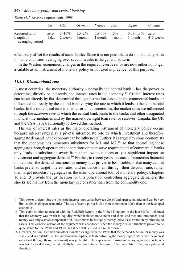
348 Monetary policy and central banking
Table 11.1 Reserve requirements, 1998
UK USA Germany France Italy Japan Canada
Required ratio zero 3–10% 1.5–2% 0.5–1% 15% 0.05–1.3% zeroLength of
averaging period1 day 2 weeks 1 month 1 month 1 month 1 month 4–5 weeks
effectively offset the results of such shocks. Since it is not possible to do so on a daily basisin many countries, averaging over several weeks is the general pattern.
In the Western economies, changes in the required reserve ratios are now either no longeravailable as an instrument of monetary policy or not used in practice for this purpose.
11.3.3 Discount/bank rate
In most countries, the monetary authority – normally the central bank – has the power todetermine, directly or indirectly, the interest rates in the economy.14 Critical interest ratescan be set directly by fiat, determined through instructions issued to the commercial banks, orinfluenced indirectly by the central bank varying the rate at which it lends to the commercialbanks. In the more usual case in market-oriented economies, the market rates are influencedthrough the discount rate at which the central bank lends to the banks and other designatedfinancial intermediaries and by the market overnight loan rate for reserves. Canada, the UKand the USA have traditionally followed this method.
The use of interest rates as the major operating instrument of monetary policy occursbecause interest rates play a pivotal intermediate role by which investment and thereforeaggregate demand in the economy can be influenced. Further, it is argued by some economiststhat the economy has numerous substitutes for M1 and M2,15 so that controlling theseaggregates through open-market operations or the reserve requirements of commercial banksonly leads to substitution away from them, without necessarily a significant impact oninvestment and aggregate demand.16 Further, in recent years, because of numerous financialinnovations, the demand functions for money have proved to be unstable, so that many centralbanks prefer to target interest rates, and influence them through their discount rate, ratherthan target monetary aggregates as the main operational tool of monetary policy. Chapters10 and 13 provide the justification for this policy for controlling aggregate demand if theshocks are mainly from the monetary sector rather than from the commodity one.
14 This power to determine the domestic interest rates varies between closed and open economies and can be verylimited for small open economies. The use of such a power is also more common in LDCs than in the developedeconomies.
15 This claim is often associated with the Radcliffe Report in the United Kingdom in the late 1950s. It claimedthat the economy was awash in liquidity, which included trade credit and short- and medium-term bonds, andmoney was only a small component of it. Restrictions in its supply merely led to its substitution by other liquidassets. This extreme version of the argument was abandoned since the money-demand functions proved to bequite stable for the 1960s and 1970s, but it can still be used in a milder form.
16 However, Milton Friedman and other monetarists argued in the 1960s that the demand function for money wasstable, and more stable than the investment multiplier, so that controlling the money supply rather than the interestrates (and through them, investment) was preferable. The experiment in using monetary aggregates as targetswas briefly tried during the late 1980s but was discontinued because of the instability of the money-demandfunction.
The central bank: goals 349
The central bank, in setting or changing its discount rate, indicates its willingness to letthe commercial banks determine the extent of borrowing from it and thereby changing themonetary base in the economy. Its target for the overnight loan rate for reserves determinesthe rate at which commercial banks borrow from each other. Any announced changes inthese rates act as indicators of the bank’s future intentions about the economy’s interestrates that it will support through its open-market operations, and therefore serve as anindicator of the future stance of monetary policy. The commercial banks and other financialintermediaries usually, though not always, follow the lead given by the discount and theovernight loan rate changes to alter their own interest rates17 – such as the prime rate, thepersonal loan rates and the mortgage rates – as well as in their purchases and sales of marketinstruments. This behavioral pattern results in a shift of the interest rates throughout theeconomy, while leaving the spread between any pair of rates to market forces. Conversely,the central bank’s refusal to change these rates in the face of rising market rates serves todampen the latter.
This discount rate is called the bank rate in Canada and the UK. In the UK, as explainedearlier in this chapter, since 1997 the Bank of England, through the Monetary PolicyCommittee, has had the operational independence to set this rate. Until 1971, a sort of cartelarrangement among the British commercial banks linked the market interest rates on varioustypes of bank deposits to the bank rate. The abolition of this cartel in 1971 made the marketrates more responsive to market forces, though the bank rate set by the Bank of Englandstill continues to be the core rate for the financial markets and changes in it are the majoroperational instrument of monetary policy. Since the British banks as a whole need to achievebalance at the end of each day, the Bank of England can choose on a daily basis the interestrate at which it will provide additional funds to the banking system. Changes in this rateprompt the banks to change the base rates at which they lend to their customers, so thatthe changes in the Bank’s own lending rate cascade through the various interest rates inBritain.
In Canada, the bank rate (at which the Bank of Canada lends to commercial banks)was set by the Bank until 1980. In the 1980s and the early 1990s, it was fixed at1/4 percent above the 91-day Treasury bill rate at its weekly auction of government bonds.Since it was above the Treasury bill rate, it was considered to be a “penalty” rate inthe sense that it imposed a net loss on the borrowing bank, which had the option ofobtaining the needed funds more cheaply by selling from its holdings of Treasury bills.The Bank influenced the Treasury bill rate through its own bids for Treasury bills. Since1994, the Bank has been setting the overnight loan rate – that is, the rate on trades inreserves – with a band of 50 basis points, as an operational target. Since 1996, the bankrate has been set at the upper limit of the operating band specified for the overnightloan rate. Setting the bank rate at this upper limit makes borrowing from the Bank moreexpensive than in the commercial market for reserves and is meant to persuade commercialbanks to meet their reserve needs through their borrowing of reserves in the privatemarkets. However, borrowing from the Bank is treated as a right of the banks ratherthan a privilege. In any case, the Canadian banks consider borrowing from the Bankof Canada as sending out a signal that they have liquidity problems and are reluctant
17 In Canada, the UK and the USA, the ability of the central bank to support its interest rate policy is credible, sothat the market rates adjust immediately to reflect the change in its rate. However, this is not necessarily the casein many other countries, especially in those with underdeveloped financial markets.

350 Monetary policy and central banking
to resort to such borrowing. Any advances are normally for only a few days and oftenovernight.
In the United States, the discount rate is frequently below the market short interest rates.Since banks can make a profit from borrowing from the Fed and then buying marketinstruments, keeping the discount rate below the market rates becomes an incentive forcommercial banks to borrow from the Fed. However, the Fed treats borrowing from it asa privilege rather than a right. Frequent borrowing from the Fed can lead to its refusalto lend again and would invite closer scrutiny of the borrowing bank’s accounts andpolicies. Further, a bank may view its borrowing as a signal to the public that it is in direfinancial need and is not able to conduct its affairs properly, so that it may be reluctant toborrow.18
A change in the discount rate can serve as an instrument of monetary policy in threerespects:
1 It affects the amount of borrowing – which changes the monetary base and the moneysupply – from the central bank.
2 Changes in it – or lack of a change when one was expected – act as a signal to the privatesector of the central bank’s intentions about monetary policy.
3 The central bank’s control over its discount rate provides it with considerable controlover the interest rates in the economy.
The latter two are now the relatively more important reasons for the use of the discountrate as an instrument of monetary policy.
Central bank as the lender of last resort
Borrowing from the central bank at the discount rate is associated with the notion of thecentral bank acting as the lender of last resort in the economy. While commercial banks withinadequate reserves can borrow from those with surpluses, a reserve shortage in the financialsystem as a whole cannot be met in this manner and could force the economy into a liquidityand credit crunch. The discount window – i.e. the ability to borrow from the central bank –is therefore a “safety” valve for the economy.
The discount window also acts as a safety valve for an individual bank that needs reservesbut is unable or unwilling to borrow from private financial institutions. However, in theUnited States, borrowing from the central bank invites the scrutiny of the central bank into theborrowing bank’s management of its affairs and acts as a disincentive to frequent borrowingfrom the central bank, as against borrowing in the market. Further, banks are not permittedto make chronic use of the discount window for meeting liquidity needs.19
18 Given such an attitude, at the time of the subprime financial crisis in August–September 2007 the Fed, whichwanted to ensure the liquidity and solvency of the banking institutions, actively encouraged commercial banksto borrow from it.
19 In Britain, discount houses usually act as intermediaries between the banks and the Bank of England. Banksthat need funds can draw down their balances at the discount houses, sell securities to them or borrowfrom them. If the discount houses need funds, they can either borrow or sell securities to the Bank ofEngland at the bank rate (also called the dealer rate). The latter method is now the more common one.The explanation for this indirect method of banks’ borrowing from the Bank of England is that directborrowing by a bank might be seen as a sign of liquidity problems and could reduce the public’s confidence inthe bank.

The central bank: goals 351
Discount rate and interest rate differentials in the economy
The central bank’s power to set its discount or bank rate does not extend over the differentialsor spreads among the various interest rates in the economy. In particular, the spreads betweenthe commercial banks’ deposit rates and the short-term market rates, such as on Treasurybills and money-market mutual funds, are still outside the direct influence of the central bankand depend upon market forces.
From the perspective of monetary theory, the determinants of the demand for M1 andother monetary aggregates are critical for the impact of monetary policy. These demandswould depend on both the levels and the differentials among interest rates. Since the latterare mainly outside the influence of the central bank, the impact of the changes in the discountrate on the demand for monetary aggregates is correspondingly reduced.
11.3.4 Moral suasion
Moral “suasion” – rather out-of-date term for “persuasion” – refers to the use of the influenceof the central bank upon commercial banks to follow its suggestions and recommendations,such as in exercising credit restraint or diverting loans to specified sectors of the economy.Such suggestions do not possess the force of law, though the threat of converting suggestionsinto legal orders, if necessary, often backs such suggestions. Moral suasion generally workswell in countries with a very small number of large banks and with a long tradition of respectfor the judgment and extra-legal authority of the central bank. Although both the UK andCanada are good examples of this, the Bank of England is especially known for its extensiveuse of moral suasion.
However, moral suasion is not generally appropriate for the large and diverse bankingsystem of the United States, though it has been tried sometimes. An example of the latteroccurred in 1965 when the President and the Federal Reserve laid down guidelines to limitforeign borrowing. This was fairly well adhered to by the member banks, but representeda rare usage of this tool in the USA. This term is also sometimes associated with the rulesimposed by the Fed on banks that attempt to borrow too frequently from it and is, therefore,associated in the US with the use of the discount window.
11.3.5 Selective controls
Selective controls are those with impact on certain sectors rather than upon the overalleconomy. A common example of these is credit controls. The usual reason for suchcontrols is that social priorities may differ from private priorities. Thus the governmentmay wish to divert funds to exports, housing, agriculture, state and local governmentsand to industries believed to be essential to national development. This can includegiving special rediscounting privileges to private commercial export bills. Some cen-tral banks also favor housing and agriculture through favorable discount provision anddirect credit controls, with such support provided under the regulations and guidelinesgiven by the central bank to the commercial banks. However, such support in theUnited States, Canada and the UK is generally fiscal, in the form of tax exemptions,subsidized loans from the government, etc., rather than being an aspect of monetarypolicy.
Another reason for selective controls is to curb the destabilizing nature of certain sectorsor to use the critical position of certain sectors for stabilization purposes. For example,

352 Monetary policy and central banking
on the former, the Federal Reserve limits the stock market credit extended by banks andbrokers on the purchase of securities by setting minimum-margin requirements. These specifythe minimum down payment at the time of purchase. This requirement was, for example,70 percent in 1968 for stocks registered on national security exchanges, so that purchasers ofsuch stocks could borrow only up to 30 percent of the purchase price from banks or brokers.The Federal Reserve can raise these requirements up to 100 percent.
Another example of such controls is those on consumer credit. These often specify, fordesignated durable consumer goods, the minimum down payment at the time of purchaseand the length of time over which the balance has to be paid. Such controls are exercisedin some countries and often go under the name of installment-credit or hire-purchasecontrols. In the USA, the Fed was given the power to impose such controls in the SecondWorld War, in the Korean War and briefly in 1948–49, but does not now possess such apower.
11.3.6 Borrowed reserves
Funds borrowed by commercial banks from the central bank are called borrowed reserves.Those acquired through their sale of securities or through the deposits with them by the publicare called non-borrowed reserves.
The distinction between borrowed and non-borrowed reserves is important since com-mercial banks usually are less willing to lend as high a proportion of the former asof the latter. This occurs since the former are borrowed for short periods and carrythe discount rate, which is usually higher than the commercial paper rate. In addi-tion, there is often a reluctance to borrow, or to borrow repeatedly, since banks viewdoing so as creating doubts in the public’s mind about the borrowing bank’s abilityto manage its affairs properly. There is, therefore, often a stigma attached to suchborrowing. Repeated borrowing also invites closer oversight, which is considered unde-sirable, by the central bank and other regulatory authorities of the bank’s investmentpolicies.
The central bank can vary the amount borrowed from it by varying the discount rate.A decrease in this rate, relative to market interest rates, makes it more tempting for banks toincrease their borrowing.
As against borrowing from the central bank, banks can borrow reserves from each otherat the Federal Funds rate in the overnight loan market for reserves; this is called the FederalFunds market in the USA. This market enables banks to lend their excess reserves to otherbanks that are short of reserves. The central bank controls both its discount rate and theovernight loan rate. The central bank manages the latter by open-market operations in thereserves market; an open-market purchase of bonds by the central bank increases the reservestraded in this market and reduces the rate.
To sum up, individual banks can borrow reserves in the overnight loan market from otherbanks that have excess reserves, through repurchase agreements with the central bank, orfrom the central bank at the discount rate.
11.3.7 Regulation and reform of commercial banks
In addition to its control of the economy through monetary policy, a major function ofcentral banking and its related regulatory authorities is to ensure the continued health of thefinancial system as a whole and of the individual banks. The latter can involve various types
The central bank: goals 353
of regulations, such as restrictions on the amount of credit and the payment of interest,20
restrictions on the type of investments that the financial institutions can make, etc.21
11.4 Efficiency and competition in the financial sector: competitivesupply of money
11.4.1 Arguments for the competitive supplies of private monies
It is a major contention of economic theory that production and exchange are at their mostefficient in perfectly competitive markets. Hence, social welfare is maximized by havingperfect competition in all sectors, including the financial one. Even if the actual marketscannot be made fully competitive, restrictions on competition are damaging to efficiency.These tenets are applicable not only to the markets for consumer and investment goods butalso to the financial markets. As a corollary, some economists have argued that the financialmarkets would be most conducive to maximizing the economy’s output if they were freefrom administrative regulations on the products that financial institutions can supply andthe prices they charge for these. The products supplied by the financial sector are essentiallytypes of financial intermediation, and involve the holdings of assets and the issue of liabilitiesby the financial intermediaries. The prices involved are interest rates in the financial marketsand service charges, etc. imposed by financial intermediaries. Hence, microeconomic theoryimplies that the various types of financial institutions should be allowed to compete with eachother in the various financial markets, such as for demand deposits, savings and time deposits,mortgages, the purchase and sale of shares, mutual funds, trusts management, pension funds,insurance, etc.
Some economists extend this argument to the proposal that the issue of money shouldalso be left unregulated and that there is no need for a central bank.22 In fact, since theexistence of such a bank with its issue of fiat money represents monopoly power over oneaspect of money, its existence and the supply of fiat money reduce social welfare. In linewith this argument, it is proposed that private, competitive firms should be allowed to issuecoins and notes. It is further argued that the power of commercial banks to create insidemoney in the form of demand deposits and other types of near-monies should not be limitedby any imposition of reserve requirements. Nor should there be regulations on the interestrates charged, on ownership, limitations on the encroachment of banks on trust companies,insurance companies, etc., by limiting the products they can supply. As we have mentionedabove, the basis for such proposals is the application of the principle of Pareto optimality ofperfect competition to the provision of monies and other financial products.
20 Until the early 1980s, the USA had imposed specific limits on the payment of interest on bank deposits. Thesewere phased out in the early 1980s.
21 In the USA, until the early 1980s, savings and loan associations were restricted to making mortgage loans. Untilthe late 1990s, commercial banks were not allowed to sell corporate securities, while investment banks coulddo so but were prohibited from commercial banking. The Fed and the Comptroller of the Currency establish theminimum capital requirements (provided by the banks’ shareholders) of the banks’ assets. To encourage trust inthe security of deposits, the Federal Deposit Insurance Corporation (FDIC) insures bank deposits to a specifiedlimit.
22 Selgin (1988) provides a spirited defense of a banking system free from regulation and dismisses the idea behindcentral bank control of the money supply that competitive commercial banks, free to issue banknotes, wouldoverissue notes and deposits for private gain.

354 Monetary policy and central banking
11.4.2 Arguments for the regulation of the money supply
While economists generally accept the propositions on the promotion of competition amongthe firms in the financial sector, few economists accept the proposals on the abolition of thecentral bank, on the elimination of its power to issue fiat money or on the elimination of itspower to monitor and regulate the financial system to ensure its continued health, etc. Thebasic reason for this stand is that the health and stability of the monetary sector is consideredto be vital to the prosperity and functioning of the macroeconomy. Further, variations in thesupply of money are taken to have a strong impact on the real sectors of the economy.
The commercial banking system is inherently fragile and based on trust by the depositorsin the viability of the institutions in which they hold their deposits. A purely competitiveand unregulated system is prone to fluctuations in the degree of this trust and thereforesusceptible to runs by depositors concerned about the security of their deposits. Two basicreasons for this are the fractional reserve practices of banks and their policy of borrowingshort and lending long. Since banks keep reserves, in cash or in deposits with the centralbank, equal to only a small fraction of their deposits, they cannot at short notice meet asudden attempt by depositors to withdraw their deposits in cash. This is further exacerbatedby the portfolio policies of banks under which large proportions of their assets are in bonds,mortgages, loans, etc., which are difficult to convert into cash at short notice or can only becashed with significant losses. Individual banks may also be tempted to engage in high-riskinvestments, with a consequent possibility of losses, which create a loss of confidence in thebank accompanied by a run to withdraw deposits from it.
Given this inherent fragility of a purely private competitive banking system, severalmeasures are taken to ensure the continuation of a high level of confidence in the bankingsystem. One of these is the insurance of individual deposits, usually to a pre-set limit,by a central deposit insurance agency. Another is having a central bank that attempts toanchor the supply of privately created inside money in the economy through its own issueof fiat money, and also attempts to control variations in the aggregate money supply in thenational interest. In addition, the central bank tries to ensure confidence in the financial sectorthrough its regulation and monitoring of financial intermediaries, especially commercialbanks since they supply the most liquid financial assets in the economy and are the creatorsof inside money.
Focusing first on the supply of fiat money by the central bank, one reason for its issueby the central bank is to anchor the privately supplied demand and other types of depositsand therefore the money-supply aggregates in the economy. Another reason concerns theseigniorage – that is, the revenue – emanating from new issues of the monetary base. Thecentral bank is a national institution and its profits are added to the fiscal revenues, sothat it seems to be the obvious recipient of such seigniorage. Further, in many low-incomeeconomies, seigniorage can be a significant proportion of national revenues and are neededfor financing government expenditures.
11.4.3 Regulation of banks in the interests of monetary policy
From the perspective of the central bank, an important aspect of its activities is its regulationof the financial institutions in the economy. Part of this regulation is aimed at the control of themoney supply in the national macroeconomic interest. Another part is aimed at maintaininga sound financial system and encouraging, if necessary, its growth to fit the financial needsof the economy. This supervision often takes the form of regulations on the ownership of

The central bank: goals 355
such institutions, forms of liabilities issued, the kind of assets held and the auditing of theiraccounts. Such supervision is only of minor interest from the standpoint of macroeconomicsprovided it is successful in maintaining a stable and adequate financial system. But it is oftena substantial part of the activities of the central bank and its related agencies, and can becritical for the solvency and efficiency of the financial system of the country.
Monetary economics is closely concerned with those regulations of the monetaryauthorities that affect the liquidity of the economy, especially as reflected in the monetaryaggregates. As discussed earlier, among these regulations the central bank often specifiesthe minimum reserves that commercial banks must maintain against demand deposits. Theinterest rate at which commercial banks can borrow from the central bank is also set bythe central bank rather than based purely on a market mechanism. There may also be otherconditions imposed on such borrowing. The maximum interest rates that commercial banksmay themselves pay on various kinds of deposits are also, in some countries, set by thecentral bank. There may be, and often are, other areas of regulation of commercial banks’behavior.
The basic reason for the close regulation of commercial banks lies in the fact that theyissue demand deposits that are a major part of the money supply, no matter how it is defined.Most of the regulations governing commercial banks are, in fact, aimed at regulating theircreation of demand deposits, with the aim of bringing the total amount of demand depositsand hence the total money supply within the control of the central bank.
Historically, banking in the British tradition arose under a set of customary practices andimposed rules that restricted commercial banks to the issue of demand and savings depositliabilities and the holding of short-term government bonds as assets. Banks were therebyconfined to the highly liquid end of the spectrum of financial assets, leaving other specializedfinancial institutions to the markets for mortgages, insurance, trusts, pension funds, etc. Inaddition, there were also restrictions on bank ownership by non-bank corporations, as wellas on the ownership of the latter by the banks.
This pattern began to change in the second half of the twentieth century, both in the issueof bank liabilities and in their portfolio of assets.23 The changes became more pronouncedduring the 1980s and 1990s, with the financial institutions increasingly being permitted toexpand into other than their traditional financial markets, as well as to own or be closelyassociated with financial institutions in other markets. These changes allowed commercialbanks to issue mutual funds, act as investment brokers for the buying and selling of shares,sell insurance and manage pension funds – and conversely to allow firms formerly engagedin these markets to offer banking services. The result by the end of the twentieth centurywas a breakdown in the USA, Canada and Britain of the barriers between types of financialinstitutions, mergers and eventually larger sizes of the financial firms, as well as much moreaggressive competition in the financial markets.
An aspect of the limitations on banks had been the regulation of the interest rates thatbanks could pay on the demand and savings deposits placed with them. Often this was anattempt to prevent too aggressive a competition for deposits and to ensure the solvencyof banks. An example of this was Regulation Q in the USA during the 1950s and 1960s,under which ceilings were imposed by the Federal Reserve on the interest rates paid by itsmembers on deposits, while many other financial institutions were not subject to such limits.In the interests of promoting competition and removing discriminatory restrictions on banks,
23 In Canada, the chartered banks were first permitted to hold mortgages in the 1950s.

356 Monetary policy and central banking
such ceilings were first gradually raised and then eliminated in the 1970s and 1980s. Theimposition of ceilings on interest rates paid by banks is now rare in financially developedeconomies, and such ceilings do not exist in Canada, the UK or the USA. But they do existin many countries, especially among the LDCs.
11.5 Administered interest rates and economic performance
Manipulating interest rates as guidance to monetary policy or as an aspect of short-termstabilization policies is quite different from setting them over long periods in order to achievesome long-run objectives. Among such objectives is that of attempting to increase the long-rungrowth rate of the economy.
Interest rates represent the cost of investment, which is the increase in the capital stock ofthe economy and an essential requirement for the growth of the economy’s output capacity.Hence, it can be argued that low rates of interest imply higher investment and thereforehigher growth rates for the economy. Many countries, especially LDCs, in the second half ofthe twentieth century, followed this reasoning to set interest rates in the organized marketsof their economies below what would have been determined in unregulated markets. Theserates were usually not adjusted to the rate of inflation, so that the interest rates that couldbe charged often fell below the inflation rate, thereby implying a negative real rate of returnon loans.
Interest is not only the cost of funds borrowed for investment, it is also the return onsavings lent through the financial markets. Neo-classical theory posits a positive relationshipbetween them, so that lower rates of interest imply lower saving. However, the empiricalsignificance of this dependence of saving on interest rates is in considerable doubt. If savingin practice does not depend on interest rates, while investment does so, it could beargued that keeping the rates of interest low would promote growth of the economy on anet basis.
Interest rates, however, also play the role of allocating funds between the various projectsand sectors of the economy. With interest rates below their levels for clearing the markets forloans, administrative mechanisms come into play to allocate the limited funds to the greaterdemand for them. Among these mechanisms are governmental or central bank regulationson the sectors, projects or firms that are to be given credit, rules of the banks themselves,favoritism of bank managers, etc. Corruption often becomes rife in such a context andbecomes a basis for the granting of loans. The end result is the misallocation of funds toprojects and firms, in which the most productive uses do not always or adequately get thefunds. Such misallocation is detrimental to the growth of the economy. Conversely, leavingthe interest rates to be determined in the open and competitive markets for loans promotes theefficient allocation of savings to the variety of investments and thereby increases the growth ofthe economy. This realization by many LDCs in the 1980s and 1990s led to the “liberalization”of interest rates – a term for lifting ceilings or setting them free to be determined by marketforces – in many of them. Such freeing of the interest rates from administrative control is veryoften part of the broader “liberalization” of the economy, through deregulation and decontrolof exchange rates, imports and exports, production and investment, etc., and has resulted inmany cases in increasing the growth rates of those economies.
While all economies have an informal financial sector in which borrowing and lendingtake place other than through the established and regulated financial intermediaries, such asector in the LDCs is larger and more significant relative to their formal financial sector.This sector is not only outside the purview of central bank control and policies, its spread

The central bank: goals 357
between the deposit rates and the loan rates is usually much larger than in the formal sector.The low deposit rates discourage saving while the high loan rates discourage borrowing forproductive investments. Therefore, while the informal sector is vital to the economies of theLDCs, policies which force savers and borrowers to the informal sector through restraints onthe formal sector tend to reduce saving and investment in these economies. This implies arecommendation for the competitive and efficient expansion of the formal sector relative tothe informal one, though not necessarily through statutory restrictions on the latter.
11.6 Monetary conditions index
In 1992, the Bank of Canada defined a Monetary Conditions Index or MCI, which is aweighted average of short-term interest rates and the trade-weighted exchange rate of theCanadian dollar. Roughly, a change in the MCI24 is specified as:
�MCI = �R + (1/3)�ρ
where R is the short-term nominal interest rate, interpreted as the 90-day commercial paperrate, and ρ is the effective exchange rate, interpreted as the exchange rate for the Canadiandollar against the 10 major (G-10) currencies. The reason for the one-third weighting of theexchange rate relative to the interest rate is the Bank of Canada’s belief, based on empiricalwork done therein, that a change in interest rates by 1 percent has three times the impact ofa corresponding change in exchange rates on aggregate demand in the Canadian economy.Given that the effect is in the same direction for both R and ρ, opposite changes in thesevariables offset each other’s effects on the economy. Hence, if an increase in the exchangerate occurs and if the Bank considers the resulting increase in the MCI to be undesirable, theBank responds by inducing a sufficient offsetting reduction in interest rates to keep the MCIunchanged. Alternatively, it can act to manipulate the exchange rate, though it normally doesnot do so.
The MCI is used as a guide for the Bank’s policies. The Bank formulates its expectations onthe state of the Canadian economy and those of its major trading partners, decides also on thedesired rates of inflation and growth in aggregate demand, and determines the target values ofMCI that would achieve these goals. Monetary aggregates, along with other macroeconomicvariables, are used as information variables. The Bank does not specify a target path for theMCI, nor set a target path for the exchange rate, nor try to ensure that its actions result in thespecific ratio of one-third in interest rate to exchange rate changes. The MCI is used as anoperational guide, but the main focus is on its goals defined in terms of aggregate demandand price stability.
The Bank sets the overnight loan rate, with a range of 50 basis points, as its operationaltarget to achieve its desired value of the MCI. It allows the financial institutions and themarkets to determine the actual amounts of the monetary aggregates on the basis of thetargeted overnight loan rate. Its money market operations are used to hold the overnight rate
24 The actual formula is:
MCI = (CP90 − 7.9) + (100/3)(lnG10 − ln 0.8676014)
CP90 is the 90-day commercial paper rate and G10 is the Canadian dollar index against G-10 currencies, withits base value for 1981 set at 1.

358 Monetary policy and central banking
in the specified range. Movements in the overnight rate in turn induce changes in the otherinterest rates and the exchange rate.
The Bank of Canada tries to influence the overnight rate through changes in the settlementbalances25 held with it by the direct clearers, mainly the commercial banks, in the Canadianpayments system. Positive amounts of these balances do not pay interest, but any negativeamounts have to be covered by overdrafts at the bank rate. While such changes in settlementbalances can be brought about by open-market operations, the Bank usually relies upon dailytransfers of government deposits between it and the direct clearers, making such transfers andthe resulting supply of settlement balances its main instrument for changing the monetarybase and exercising control over the economy.
The Bank of Canada believes that uncertainty is inimical to the proper functioning of thefinancial markets and the efficiency of the economy, and that the uncertainty of monetarypolicy can adversely affect saving and investment in the economy. In an attempt to reduce suchuncertainty, changes in the target range for the overnight rate are immediately made knownto the public, and the intended course of the monetary policy of the Bank is continuouslyexplained to the public through publications and speeches of the Governor of the Bank andits officials.
11.7 Inflation targeting and the Taylor rule
Currently, the central banks of Britain, Canada, the USA and many other countries are saidto follow “inflation targeting,” which is the pursuit of an inflation target. However, in reality,they have adopted a Taylor rule (Taylor, 1993; also see Chapters 12 and 13) of the generalform:
rt = r0 +α(yt − y f ) +β(πt −πT) α,β > 0 (1)
where r is the real interest rate to be set by the central bank, y is real output, y f is full-employment output, π is the actual inflation rate, πT is the inflation target of monetarypolicy and the subscript t refers to period t. πT is called the target inflation rate. Similarly,y f is the target output level. (yt − y f ) is (minus of) the output gap. r0 should be the long-runreal interest rate.
The Taylor rule embodies two objectives: stabilizing inflation at its target rate andstabilizing output at its full-employment level. While movements in the inflation rate andoutput are, on average, positively correlated, they are not necessarily so over short periods.Under this rule, monetary policy raises the interest rate if inflation is above target and output isabove its full-employment level. Some proposals for the Taylor rule include other variables,such as the exchange rate.
Note that, in practice, central banks set the nominal interest rate rather than the real one.Consequently, the Taylor rule implies that if πt −πT > 0, the nominal rate would rise morethan the inflation rate, and if πt −πT < 0, the cut in the target real rate would mean that thenominal rate would fall more than the inflation rate. Such a policy is one of “leaning against
25 Settlement balances is the term being currently used to designate the deposits held by designated financialinstitutions, called direct clearers with the Bank of Canada. In the absence of any legally required reserves,these deposits are held voluntarily by the direct clearers and are used to settle their daily imbalances in receiptsand payments against each other. This settlement is done through their accounts at the Bank.
The central bank: goals 359
the wind.” For any given inflation rate, the greater the value of β, the larger will be the changein the real and nominal rates and the stronger the movement to stabilize the inflation rate atits target value.
While monetary policy can use either the interest rate or some monetary aggregate, orsome combination of the two, central banks in Britain, Canada and the USA, as well as inmany other countries, use the interest rate, rather than a monetary aggregate, as the operatingtarget of monetary policy, though the European Central Bank also monitors movements inmonetary aggregates, especially M3, as part of its formulation of monetary policy. The interestrate usually targeted by central banks is the overnight loan rate in the market for reserves,but it could also be the discount/bank rate at which the central bank lends to commercialbanks.
A major advantage of specifying the inflation target in the Taylor rule is that itencourages the transparency of monetary policy and anchors inflation expectations, whichprovides guidance for wage demands, investment plans, etc. Since the 1980s, central banks’achievement of their low inflation targets has increased the credibility of their targetsand policies, which has meant that the public’s inflationary expectations are now closelydetermined by the central bank’s inflation targets (see Chapter 12 on the credibility ofmonetary policy).
Empirically, while none of the central banks has announced its form of the Taylor ruleor even a commitment to it, this rule has performed quite well in econometric studies forBritain, Canada and the USA, as well as for many other countries. Its use has been creditedwith a reduction in inflation from high levels during the 1970s and 1980s to the current lowlevels. It has also been credited with reductions in the volatility of inflation since the 1980s(Clarida et al., 1998; Sims, 2000; Moreno and Rey, 2006). Chapters 13 and 15 provide furtherdiscussion and references on the Taylor rule.
11.8 Currency boards
Some countries, more so in the past but rarely nowadays, had currency boards instead ofcentral banks.26 With a currency board, the country maintains a fixed exchange rate againsta designated foreign currency, and the monetary base – a liability of the currency board – isbacked by its foreign exchange reserves. As these reserves increase – for example, througha balance-of-payments surplus – the currency board increases the monetary base and themoney supply in the economy increases. Conversely, as foreign exchange reserves fall, themonetary base and the money supply are decreased. Other than this, the currency board doesnot have discretion to change the money supply or manage interest rates and therefore cannotpursue domestic monetary policies.
Currency boards were common in the colonies of imperial countries – for example, the UK –during the first half of the twentieth century. They were a means of linking the currency andeconomies of the colonies to those of the imperial country. Further, if the imperial currencywas under the gold standard – that is, with its value fixed in terms of gold – the coloniesalso indirectly adhered to the gold standard. Such currency boards were usually replaced bycentral banks on independence. In other cases, countries, though independent, maintainedcurrency boards with a strict adherence to the gold standard, implying a fixed value of thedomestic currency in terms of gold.
26 As of 1998, currency boards existed in Hong Kong, Argentina, Estonia and Lithuania and a few other countries.

360 Monetary policy and central banking
Note that most of the aspects of this chapter, bearing on the goals, instruments and targetsof monetary policy, do not apply to currency boards.
Conclusions
The monetary sector is central to modern economies and its proper functioning is critical tothe levels of employment, output and growth. As an illustration of this importance, it is nowgenerally agreed that monetary failure caused, or was a major main contributor to, the GreatDepression of the 1930s (Friedman and Schwartz, 1963).
The central bank is the custodian of the health, efficiency and performance of the financialsector. The monetary policy pursued by the central bank is therefore fundamental to theperformance of the economy. This chapter has shown that the goals and the favoredinstruments of central banks have varied over time and differ among countries. Currently, thedominant belief of most central banks is that they can best promote output, employment andgrowth through fairly stable prices. In particular, the belief is that continual or discretionaryattempts to increase aggregate demand through monetary policy do not yield higher outputor reduce business fluctuations over time. Further, monetary policy acts on the economywith a sufficient lag so that, with the future course of the economy being difficult to predictaccurately, the proper formulation of monetary policy is an art and, as such, potentiallysusceptible to error.
In the 1990s the dominant goal, pursued in the European Union, Canada, New Zealand,the UK, the USA, and many other countries, was that of price stability, encompassed in thenotion of inflation targeting, which is the maintenance of a low rate of inflation (about 1 to3 percent). Given the long-run neutrality of money, this goal is sometimes conveyed as anultimate goal and at other times as an intermediate goal towards improving the growth ratesof output and employment in the economy. For Canada, the European Union, New Zealandand the UK the target for the inflation rate is explicitly announced, whereas the USA doesnot announce – and therefore, does not give an explicit pre-commitment to – a pre-specifiedinflation target. However, empirical studies have shown that the Taylor rule (see Chapters 13and 15) performs quite well for all these countries, so that the monetary policies of the centralbanks were not aimed exclusively at an inflation target but rather at the deviations of outputand inflation from their desired long-run levels.
The use of interest rates as operational targets is to be distinguished from a policy offixing them administratively for long periods and at relatively low levels, with the ostensiblepurpose of promoting growth. This was done in many LDCs during the 1970s and 1980s,though there is currently a trend away from this practice. The interest rate is the opportunitycost of loans and should, for the proper allocation of funds in the economy, be determinedby competitive forces in the open markets. Setting them or setting artificially low ceilingson them by administrative action introduces inefficiencies into the financial structure ofthe economy, inimical to the optimal generation of savings, as well as to their allocationby the financial institutions optimally to investment among the sectors of the economy.27
LDCs are especially prone to setting artificially low interest rates on loans in the organized
27 The continual revision of such ceilings in the light of changes in the market interest rates, as is done insome countries, does moderate this argument. But since they are invariably delays and rigidities in changingadministered interest rates, such rates almost always introduce some inefficiency in the financial sectors of theeconomy.

The central bank: goals 361
financial sector. This could also happen in developed economies in which the interest rate isused as an operating target.28
Summary of critical conclusions
❖ Historically, most central banks have had the mandate to pursue a number ofmacroeconomic goals, including price stability, low unemployment and high growth.Achievement of multiple goals is only possible if the economy does allow such a possibilityand the policy maker has enough policy tools.
❖ Since the early 1990s, many economists have recommended – and many central banks havefollowed – inflation targeting. However, the Taylor rule, embodying a trade-off betweendeviations of inflation and output from their desired long-run levels, better describes thecurrent pursuit of monetary policies.
❖ While the interest rate was historically the operating target of monetary policy, a diversion tomonetary targeting occurred during the late 1970s under the impact of St Louis monetarism.This experiment was not considered to be a success in most countries.
❖ Most Western countries have reduced percentage reserve requirements on commercialbanks to levels that are close to zero, which eliminates changes in these requirements as atool of monetary policy.
❖ Since the early 1990s, the most common tools of monetary policy in developed economieshave been changes in interest rates, supported by changes in the money supply induced byopen-market operations and borrowing from the central bank.
Review and discussion questions
1. Historically, what goals were mandated for central banks? Why have the goals pursuedin recent years been narrowed to “inflation targeting”?
2. Can central banks pursue and achieve multiple goals or must they be confined solely tofighting inflation? What goals are embedded in the Taylor rule? Discuss.
3. What is the lender-of-last-resort function of the central bank in modern economies?What is its justification? Should commercial bank borrowing from the central bank be aprivilege or a right? Discuss.
4. Should the United States and Canada follow the example of Britain in giving thegovernment the power to set the ultimate goal or goals of monetary policy, while leavingthe implementation of these to the central bank? Or should Britain follow the exampleof the United States and Canada on this issue? Discuss.
5. What are the tools available to the central bank for controlling the money supply? Discusshow manipulation of each of these tools will change the money supply and how reliableeach tool is likely to be.
6. Why has the use of changes in reserve requirements as a tool of monetary policybeen largely abandoned in Western economies? What were the reasons for the virtualelimination of reserve requirements? Is there a case for their revival and usage as a toolof monetary policy in the context of the country you live in? In LDCs?
28 Many economists contend that the Fed maintained interest rates too low during 2002–2007, thereby contributingto high aggregate demand – as well as to the housing price bubble during these years and its collapse in 2007.

362 Monetary policy and central banking
7. How can central bank discounting cause procyclical movements in the money supply?How can the central bank eliminate such a movement? Discuss.
8. The pursuit of selective fiscal policies in the form of tax exemptions and subsidies iscommon in almost all countries, whereas the usage of monetary policy on a selectivebasis is rare in the financially developed economies. Why? Should the use of selectivemonetary policies be abandoned for the LDCs also?
9. Suppose that for a given economy the preconditions for the effective pursuit of openmarket conditions are not met. What monetary policy tools are likely to be the mosteffective ones for such an economy? Relate your recommended tools to the preconditionsthat are not met.
10. What does financial intermediation mean? What are the different financial intermediariesin your country. Which of their liabilities would you classify as components of themonetary aggregates? Discuss.
11. Suppose that instead of imposing reserve requirements on demand deposits in thecommercial banks, the central bank does the following: require automobile owners tohold $500 of non-interest-bearing deposits with the central bank.
i. How would the determination of the price level differ between the two arrange-ments?
ii. How would the real consequences of the two arrangements differ?iii. Are there any special characteristics of demand deposits or any other reasons that
make one of these arrangements preferable to the other?
12. “Due to fairly radical changes in the structure of the financial sector in recentdecades, the importance of demand deposits has declined considerably and the roleof commercial banks has changed dramatically. The main stream of monetary theoryand practice continues to be directed mainly at demand deposits and commercialbanks as purveyors of checking accounts. But checking deposits are simply onekind of liquid asset and banks are simply one kind of intermediary. Therefore, tosingle out checking deposits and commercial banks for special analytical treatmentis mistaken. Effective control of the economy by the central banks requires controlover all types of liquid assets and over the liabilities of all financial intermediaries.”Discuss.
13. “The standard practice of governments whereby they define the monetary unit isunnecessary and undesirable. The private sector should be encouraged to choose itsown standards in a free competitive market” (Friedrich Hayek). Discuss.
References
Clarida, R., Galí, J. and Gertler, M. “Monetary policy rules in practise: some international evidence.”European Economic Review, 1998, 42, pp. 1033–67.
Friedman, M. “Nobel prize lecture: inflation and unemployment.” Journal of Political Economy, 85,1977, pp. 451–73.
Friedman, M. and Schwartz, A.J. A Monetary History of the United States. Princeton, NJ: PrincetonUniversity Press, 1963.
Goodhart, C.A.E. “Central banking.” The New Palgrave Dictionary of Economics: Money. London:Macmillan, 1989.
Goodhart, C.A.E. The Central Bank and the Financial System. Cambridge, MA: MIT Press, 1995.Moreno, A. and Rey, L. “Inflation targeting in Western Europe.” Topics in Macroeconomics. Berkeley
Electronic Press, 6, 2006, Article 6.

The central bank: goals 363
Selgin, G. The Theory of Free Banking: Money Supply under Competitive Note Issue. Totowa, NJ:Rowman and Littlefield, and the Cato Institute, 1988.
Sims, C.A. “A review of monetary policy rules.” Journal of Economic Literature, 39, 2000,pp. 562–6.
Taylor, J.B. “Discretion versus policy rules in practise.” Carnegie–Rochester Conference Series onPublic Policy, 39, 1993, pp. 195–214.

12 The central bankIndependence, time consistency andcredibility
This chapter focuses on the analytical treatment of three major issues: independence ofthe central bank, time consistency of policies and the credibility of central bank objectivesand policies. Assuming a potential for tradeoffs among goals, this chapter examines thedetermination of the choices made and the potential for conflicts among the monetary andfiscal authorities. This discussion leads to the examination of the independence of centralbanks from governments and legislatures.
This chapter also shows the superiority of intertemporal optimization policies to myopicones, which can have an inflationary bias. Intertemporal optimization over time provides twotypes of policy approaches. One of these is the time-consistent one in which the policy pathfor the current and future periods is derived only once and followed for all future periods. Thesecond approach allows reoptimization every period with an unchanging objective function.
Finally, the chapter investigates the superiority of prior commitment to future objectivesand policies, and credibility of the central bank.
Key concepts introduced in this chapter
♦ Preferences over goals♦ Economy’s constraints on the tradeoff among goals♦ Conflicts among policy makers♦ Central bank independence♦ Myopic optimization♦ Time consistency of policies♦ Reoptimization with an unchanging objective function♦ Credibility of policy and commitment
This chapter focuses on several issues important to the formulation of monetary policy bythe central bank. Among these are the choice among goals and the possibility of conflictsbetween the monetary and fiscal authorities in the attainment of their desired targets and goals.In cases of such conflicts, the ability of the central bank to pursue its own choices becomesimportant and is discussed under the heading of the independence of the central bank.
The other two major issues addressed in this chapter are those of the time consistencyand credibility of policies. The time consistency of monetary policies deals with thequestion of whether the central bank should determine its policies for the future periodswithin its horizon and stick to them, or should retain discretion to reformulate its policies

The central bank: independence 365
as time passes. Discretionary policies can be arbitrary ones, be derived from one-period(“myopic”) optimization or be based on continual intertemporal reoptimization as each periodpasses. Related to the issue of time consistency of policy is the important one of maintainingthe credibility of the central bank among the public and the consequences of a failure tomaintain credibility.
Section 12.1 presents the optimizing framework for making choices among goals andtargets. This analysis follows the utility maximization approach, subject to the constraintson targets set by the economy. Section 12.2 considers the case of two policy makers, thecentral bank in charge of monetary policy and the government in charge of fiscal policy,and shows that there is considerable scope for conflict in the pursuit of these policies.Section 12.3 addresses the important issue of the independence of the central bank from thegovernment. Section 12.4 presents the analyses of policies based on myopic optimization,intertemporal time consistent optimization and intertemporal reoptimization. Finally, Section12.5 examines the credibility of central bank policies and their effectiveness, as well asthe impact on credibility of gradualist versus cold-turkey attempts to lower the rate ofinflation.
12.1 Choosing among multiple goals
As discussed in the last chapter, economic theory and central bank beliefs prior to the 1980shad indicated that several goals could be addressed through monetary policy. For the analysisof such a possibility, this section assumes that the central bank has a multiplicity of goals.Focusing only on the primary goals, the instruments available for achieving the multiple goalsare severely limited in number and scope so that not all the goals can be attained through theuse of monetary policy. Therefore, the central bank has to make a choice among its desiredgoals or combinations of them.
Assume that the central bank’s preferences over the goal variables are consistent andtransitive, so that there exists an ordinal utility function over the goal variables. Fordiagrammatic analysis, the indifference curves between any given pair of these variablescan be derived from this utility function.
Choosing between inflation and unemployment
The goal variables of many central banks include the rate of inflation and the unemploymentrate, which can be a goal variable in its own right or a proxy for the output gap. Assume thatthe central bank’s preferences over these variables can be encompassed in an objective/utilityfunction of the form:
U = U (π,u) (1)
where π is the rate of inflation, u is the rate of unemployment, and Uπ ,Uu < 0. Hence,the indifference curves in the (π , u) space are negatively sloped. Further, it is reasonableto assume that the undesirability – that is, disutility – of each variable keeps on increasing,ceteris paribus, with higher levels of it, so that Uππ ,Uuu < 0. Hence, as the rate of inflationrises, the central bank is willing to accept a higher marginal increase in the unemploymentrate in order to prevent a further rise in the rate of inflation, so that the indifference or tradeoffcurves between the rates of inflation have the usual convex shape, as shown in Figure 12.1by the curves ICB and I′CB. A host of such curves exist, with a curve passing through every

366 Monetary policy and central banking
p
u
PCIG
I ′CB
ICB
p∗CB
u∗CB
Figure 12.1
point in the quadrant. Note that since being on a lower curve is preferred to being on a higherone, the central bank will want to be on the lowest attainable indifference curve.
A common variant of the above objective function is:
U = U (π −π∗,y − yf) Uπ#,Uy# < 0 (2)
where π# = π −π∗,y# = y −yf, so that π# and y# are the respective gaps between the actualand the desired values of π and y. Since the central bank’s choices are limited by constraintsimposed by the economy on the values of π and u that can be attained, the central bank’sdecision problem is optimization of utility subject to these constraints.
The preceding discussion has been in terms of a general utility function. Current monetaryand macroeconomic theory prefers to use an intertemporal, as against a myopic (one period)utility function. The choice between intertemporal and myopic optimization is discussed laterin this chapter in the context of the time consistency debate. Chapter 15 re-visits these issuesin the discussion on the Phillips and new Keynesian curves.
General analysis of the choice among goals when the economy allows a tradeoff
The preceding utility function can be generalized to the case of n variables. The formalanalysis of this general case assumes that the central bank has a utility function:
U = U (x1, . . .,xn) (3)
At this stage, we assume that the central bank’s choice is subject to only one constraint, whichhas the form:
f (x1, . . .,xn;z,Ψ ) = 0 (4)
where:xi = ith goal variablez = vector of instruments available to the central bankΨ = vector of exogenous variables.

The central bank: independence 367
The goal variables can be levels of variables, their growth rates or even such variablesas the output gap and the “inflation gap,” where the gaps are deviations from their desiredlevels. U (.) represents the central bank’s preferences over its goals. These depend uponthe organizational structure of the central bank, the interactions between the policy makers,their perceptions of society’s goals, the structure of the economy and of what is achievable,political pressures, and so on. Equation (4) should properly specify the actual form of theconstraint. However, this form is usually not known, so that the form of the constraint usedby the central bank is that perceived by it and is based on its knowledge of the structure of theeconomy and the political and social environment. However, under imperfect informationon the economy, the relevant constraint perceived by the central bank may not necessarilyor even usually be the actual one imposed by the economy.1 The central bank is taken tomaximize (3) subject to (4) in order to determine its optimal choices among the goals.
The basic objections to the use of a preference function are to its requirements ofconsistency and transitivity in making choices. The central bank’s decisions are made bya host of individuals and its major choices, if consciously made, are by a group. Such groupdecisions in a democratic framework need not necessarily be consistent and transitive, evenat a point in time, let alone over time. Further, the policy makers in the central bank changeover time, so that its preferences are likely to shift over time. Hence, one must be cautious inexplaining the choices among goals made by the central bank within a static utility functionand its implied set of indifference curves, especially when there has been a change in itsmanagement.
In spite of these objections, the preceding analysis furnishes considerable insights into theproblem of choice among alternative goals. Empirical and descriptive studies using data upto the 1980s indicate considerable validity for this analysis and show that the central banksoften manipulated their policy instruments, such as the monetary base and interest rates, ina systematic fashion to address their chosen goal levels.
Choices under the economy’s supply constraint
There are several forms of the economy’s supply constraint relating u and π . Of these, thePhillips curve (see Chapter 15) was proposed in 1958 by A.W. Phillips and soon beganto be treated as the economy’s constraint between inflation and unemployment. Its generalform was:
u = f (π ) f ′ < 0 (5)
This constraint allows the central bank to trade between higher inflation and lowerunemployment. Optimization of the utility function (1) subject to (5) yields the optimalvalues of π and u, with higher inflation rates yielding lower unemployment.
While most Keynesians of the 1960s and 1970s accepted some form of (5) as the economy’sconstraint and explained central banks’ monetary policy under it, many economists, especiallyneoclassical ones, believed that the economy had a vertical Phillips curve for the long run.Their arguments were subsequently refined by Friedman and Lucas (see Chapters 8 and 14)
1 Therefore, there is ample scope for wide differences among political parties, economists, political scientists andthe public, etc., on what they believe can be accomplished by any given set of policies, which may differ fromwhat in fact can be accomplished.

368 Monetary policy and central banking
who asserted that the proper form of the economy’s constraint was the Friedman–Lucasaggregate supply curve, also known as the expectations-augmented Phillips curve. Thisconstraint, under the assumption of rational expectations, is of the form:
(u − un) = f (π − Eπ ) f ′ < 0 (6)
where du/dEπ= 0 and the use of a systematic monetary policy by the central bank changesboth π and Eπ by the same extent, so that (π −Eπ ) would not change. This constraint belongsto the modern classical approach (see Chapters 1 and 14). According to it, unemployment canonly be made to deviate from its natural rate through unanticipated inflation, which, givenrational expectations, requires a random monetary policy. Therefore, there is no tradeoffbetween these variables which systematic monetary policy by the central bank can exploit,so that the recommendation is that the central bank should adopt the target of price stability.Many central banks adopted this economic framework in the 1990s and some economistsadvocated that price stability or a low rate of inflation should be the central bank’s onlygoal variable. Further, in the 1990s, many central banks came to believe that higher ratesof inflation have little to contribute in terms of higher output, while they could lead toescalating inflation and lower output. At the same time, negative rates of inflation areconsidered inimical to full employment because of their potential for causing a recession.Given these beliefs, the utility-maximizing goal rate of inflation would be zero, or a lowpositive inflation rate.
As pointed out earlier, some economists choose to work with the objective function:
U = U (π −π∗,y − yf) Uπ#,Uy# < 0 (7)
where π# = π−π∗,y# = y−yf, so that π# and y# are the respective gaps between theactual and the desired values of π and y. Given this objective function, maintaining theexpectations-augmented Phillips curve as the constraint, as well as assuming that the centralbank does not want to or cannot fool the public by causing unanticipated inflation, impliesthat the optimal values of inflation and output are π∗ and yf, of which the former can beachieved through systematic monetary policy. The latter is not affected by monetary policybut is determined by the long-run performance of the economy.
However, for imperfect competition and price rigidities, the new Keynesians proposea different form of the supply constraint (see Chapter 15) to (6), so that their policyrecommendations would differ from the above. This form is known as the new KeynesianPhillips curve.
The preceding discussion of the Phillips curve, its expectations-augmented version andthe new Keynesian Phillips curve illustrates that the accurate form of the economy’sconstraint is usually not known. There are continual disputes among economists evenabout its general form, less alone the specific one with numerically specified values of theparameters.
12.2 Conflicts among policy makers: theoretical analysis
Another application of the utility approach is to the choices exercised by several (at leasttwo) policy makers over the same set of goal variables. Different policy-making bodies in theeconomy are likely to have different preference functions and hence different indifference

The central bank: independence 369
curves between any given pair of variables. Therefore, the formal optimization analysis fortwo policy makers A and B would be:
(1) For policy maker A:
Maximize UA = UA(x1, . . .,xn) (8)
subject to A’s perceived constraint:
f A(x1, . . .,xn;z,Ψ ) = 0 (9)
(2) For policy maker B:
Maximize UB = UB(x1, . . .,xn) (10)
subject to B’s perceived constraint:
f B(x1, . . .,xn;z,Ψ ) = 0 (11)
The superscripts A and B refer to the policy maker. Since both the utility functions and theperceived constraints can differ, the optimal values of the goals for xA
1 , . . .,xAn will differ
from xB1 , . . .,xB
n , so that working at cross purposes can be a common phenomenon, ratherthan a rare occurrence, among policy makers in the economy. This possibility depends uponthe differences in the utility functions, becoming reinforced by any differences in the policymakers’ perceptions of the actual present and expected course of the economy. In most cases,such conflicts in the understanding of the economy and desirable tradeoffs among objectivesby the fiscal and monetary authorities of a given country tend to be mild. However, they canerupt into open and sometimes acrimonious public debate in times of radical economic andpolitical change and of differences in ideology.
The two principal tools for the control of aggregate demand are monetary and fiscal policies.In a country with an independent central bank, monetary policy is in the control of the centralbank whereas fiscal policy is in the hands of the legislature and the government. The latterdepends on the public for electoral support and generally tends to attach greater undesirabilityto increases in unemployment relative to increases in inflation than does the central bankwhich is usually more vitally concerned with inflation. Formally, in terms of the marginalrates of substitution of the two policy makers, ∂π/∂uCB < (∂π/∂u)G, where CB stands for thecentral bank and G for the government, implying (Figure 12.2) that the indifference curvesof the central bank are steeper than those of the government. This implies that for a givenconstraint f (π,u) = 0, the central bank would adopt a monetary policy aimed at achievinga lower rate of inflation than the government. This is illustrated in Figure 12.2 in whichthe central bank’s indifference curves are shown by ICB, the government’s by IG, and theeconomy’s (common) constraint is shown by PC. The central bank’s optimal choice is for(π∗CB, u∗CB) and the government’s is for (π∗G, u∗G), implying a more expansive stance bythe government for the economy relative to that by the central bank. There therefore existsin this case a conflict between the central bank and the government on the desired rates ofinflation and unemployment for the economy. If each tries to achieve its goals through thepolicy at its command, neither will achieve their own goals.
Over time, the political process may bring about a narrow “consensus range” within whichthe differences between the central bank and the government over the desired goals are
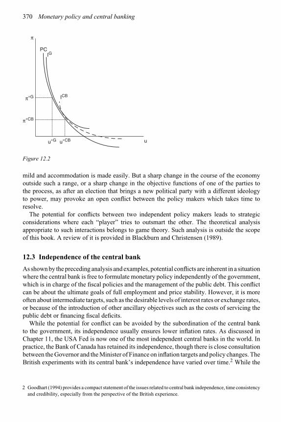
370 Monetary policy and central banking
π
u
PCIG
ICBπ∗G
π∗CB
u∗G u∗CB
Figure 12.2
mild and accommodation is made easily. But a sharp change in the course of the economyoutside such a range, or a sharp change in the objective functions of one of the parties tothe process, as after an election that brings a new political party with a different ideologyto power, may provoke an open conflict between the policy makers which takes time toresolve.
The potential for conflicts between two independent policy makers leads to strategicconsiderations where each “player” tries to outsmart the other. The theoretical analysisappropriate to such interactions belongs to game theory. Such analysis is outside the scopeof this book. A review of it is provided in Blackburn and Christensen (1989).
12.3 Independence of the central bank
As shown by the preceding analysis and examples, potential conflicts are inherent in a situationwhere the central bank is free to formulate monetary policy independently of the government,which is in charge of the fiscal policies and the management of the public debt. This conflictcan be about the ultimate goals of full employment and price stability. However, it is moreoften about intermediate targets, such as the desirable levels of interest rates or exchange rates,or because of the introduction of other ancillary objectives such as the costs of servicing thepublic debt or financing fiscal deficits.
While the potential for conflict can be avoided by the subordination of the central bankto the government, its independence usually ensures lower inflation rates. As discussed inChapter 11, the USA Fed is now one of the most independent central banks in the world. Inpractice, the Bank of Canada has retained its independence, though there is close consultationbetween the Governor and the Minister of Finance on inflation targets and policy changes. TheBritish experiments with its central bank’s independence have varied over time.2 While the
2 Goodhart (1994) provides a compact statement of the issues related to central bank independence, time consistencyand credibility, especially from the perspective of the British experience.

The central bank: independence 371
Bank of England was historically a quasi-private bank, independent of the government, thedominance of the government over the Bank of England was legislated by the Bank Actof 1946, which nationalized its ownership. It also allocated the choice over the goals andtargets of monetary policy to the Chancellor of the Exchequer, representing the government,leaving the Bank of England with a consultative and implemental role. In 1997, the Bankof England and the Monetary Policy Committee were given operational independencetoward the achievement of the inflation target set by the Chancellor. These arrangementswere enacted into law by the Bank of England Act of 1998. Under it, the Chancellorsets the goals of monetary policy – currently a target value of the inflation rate – andthe Bank and the Monetary Policy Committee have the responsibility of formulating andimplementing policies for their achievement. Therefore, as of 1999, Britain allocates onlyoperational but not goal independence to its central bank. At a formal level, this degreeof independence differs from that of the central banks of the Canada and the USA, whichpossess both goal and operational independence. The Bank of England is now one of thenational banks within the federal structure of the European System of Central Banks. TheEuropean Central Bank (ECB) is, by legislation, independent of the government of theEuropean Union.
In many other countries, including many LDCs, the subordination of the central bank tothe fiscal authorities is fairly common in practice, even if the legislation formally makes thecentral bank independent of the government.
Such lack of independence of the central bank in the formulation and pursuit of monetarypolicy represents a threat to the pursuit of appropriate monetary policies for price stability.In fact, many empirical studies for the 1970s and 1980s showed that countries that retainedactual independence of the central bank from the government tended to have lower rates ofinflation; conversely, the lack of independence resulted in higher inflation rates (Alesina andSummers, 1993).
The trend since the 1980s has been strongly towards granting greater or completeindependence. By now, almost all developed economies have independent central banks.
Development strategies in LDCs, financing fiscal deficits and central bankindependence
The issue of central bank independence takes on another dimension in countries that incurlarge and persistent deficits but do not possess adequate capital markets to finance themthrough new issues of public debt, and need the central bank to do so through an expansionof the monetary base. This often happens during wars, even in the developed economies, buthas occurred most noticeably in recent decades in the LDCs.
LDCs tend to have low output per capita and are not able to raise adequate tax revenuefor their desired levels of public expenditures. The latter are in many countries swollen bytheir plans for public development projects or the deficits of their public sector undertakings.Further, their domestic financial markets are under-developed and cannot support much, ifany, government borrowing, and their ability to borrow abroad is also severely limited. Asa result, many LDCs resort to increases in the monetary base, either directly or indirectlythrough the compulsory sale of government bonds to the central bank. This process requiresthe subservience of the central bank and its policies to the fiscal needs of the government,and destroys the central bank’s independent control over monetary policy.
Whether such an arrangement is advantageous to the economy is in considerable doubt.On the positive side is the financing of public projects that would otherwise not have been

372 Monetary policy and central banking
financed, or provision for social objectives such as health, education and alleviation ofpoverty. On the negative side is the subordination of increases in the monetary base to budgetdeficits, with the consequent loss in control by the central bank over monetary policy andover aggregate demand and inflation in the economy. From the perspective of price stability,this loss of independent control of the monetary base by the central bank severely limits itscapacity to control inflation. Many empirical studies have documented that countries withindependent central banks, which are not necessarily obliged to finance the budget deficits,tend to have lower rates of inflation. Another negative aspect of this arrangement is that theborrowing for the public projects thus financed is not done in competitive markets at market-determined rates. Hence, allocative efficiency suffers and private projects that could be moreefficient and could have been undertaken are crowded out. These efficiency losses could beconsiderable and, in the opinion of many economists, have contributed to the low growthof those LDCs that resorted heavily in the past to the financing of governmental deficits byincreases in the monetary base.
While few central banks in developing countries were effectively independent ofthe government prior to the 1990s, the economic arguments and evidence supportingindependence have since then led many developing countries to grant much greaterindependence to their central banks.
Central bank independence in practice
A country can have laws formally legislating the independence of its central bank from thegovernment. However, its independence in practice will usually also depend on additionalfactors, such as the mode of appointment of the bank’s directors, the duration and terms oftheir appointment, their relationship with those in the legislature and the government, powerpolitics, and how the spirit of the law is respected in the country in question. On this point,Cukierman et al. (1993) reported that while legal independence was an important determinantof inflation in the industrialized economies, with a negative coefficient, the rate of inflationwas strongly and positively related to the central bank governor’s rate of turnover, ratherthan to legal independence, in the developing economies.
Hence, legal independence does not always ensure factual independence. In general,the factual independence of the central bank from the government normally depends onits acceptance by the main political parties of the country and substantial support for itamong the public. This acceptance, in turn, depends on the rule of law in the country,the belief in the integrity and commitment of the central bank directors and governorsand the past record of the central bank, as well as the transparency of its policies and itsaccountability.3
Goodhart (1994) finds that central bank independence, if effective, is a way of makingits commitment to price stability more credible and makes the achievement of low inflationmore likely. But he finds no evidence that it lowers unemployment or the “loss ratio,” definedas “the number of extra man-years of unemployment necessary to lower inflation by one percent” (p. 68). Eijffinger and de Hahn (1996) concluded from their review of empirical studiesthat the weight of empirical evidence does support the claim that independence of the centralbank from the government does reduce inflation. However, such independence does not
3 Eijffinger and de Hahn (1996) provide a thorough review of the issues and empirical studies on central bankindependence.

The central bank: independence 373
seem to have increased employment and growth. Further, there were higher rather than lowerdisinflation costs associated with independent central banks.
12.4 Time consistency of policies
The proper design of monetary policies4 over time requires that the central bank havean intertemporal objective function to rank alternative policies and know the economy’sconstraints, as well as possess knowledge of the current and future responses of the economyto its policies and how it intends to set its policies in the future.
A time-consistent policy path is one that is derived from optimizing an intertemporalobjective function subject to the appropriate constraints describing the behavior of theeconomy, with the optimal policy path over time derived once-for-all and followed as timepasses. The latter requires a commitment to pursue the derived set of policies, both in thecurrent and future periods, so that the central bank would have to resist the temptation and thepolitical pressures to deviate from this path. Hence, time consistency of policies is related tothe issues of the independence of the central bank and of a commitment regime under whichthe central bank will maintain a pre-set future policy path.
To illustrate, suppose that the central bank does want to pursue time-consistent policieswith the long-term goal of price stability, while the government has the objective ofgetting re-elected which, given a short-run Phillips curve tradeoff between inflation andunemployment, is enhanced by short-term inflationary monetary policies. The central bankis more likely to resist pressure from the government if it is independent of the politicalprocess. Therefore, the independence of the central bank from the government and thelegislature improves its ability to pursue time-consistent policies. This reasoning is nowwidely accepted, so that, as pointed out earlier, the central banks of most developedcountries and of many emerging ones now possess a high degree of independence of thegovernment.
Time-consistent policies are generally compared with discretionary policies. Discretionarypolicies allow the central bank discretion to deviate or not from the pre-set policy path. Underthem, the central bank retains the right to pursue policies as it thinks fit at the time the policiesare pursued. The set of policy types is:
1 Purely arbitrary policies.2 Myopic (one period) policies. These are derived from myopic (short-term, usually one
period) optimization with short-term goals subject to the constraints for the current periodonly and with expectations taken as exogenously given. Further, under this procedure, thepolicy maker does not give any advance commitment, even on maintaining the objectivefunction, on its future policies.
3 (Intertemporal) reoptimization policies. These policies are derived from intertemporalreoptimization each period for that period and future ones, with an unchangedintertemporal objective function, which is maximized subject to the long-run or multi-period constraints specified by the structure of the economy. Under this procedure, thepolicy maker gives a commitment to maintain the same intertemporal objective functionover time, but the relevant constraints can shift with the passage of time. The optimal
4 Fischer (1990) provides an excellent review of the literature on different types of policies, their evolution andfoundation, as well as a comparison of time-consistent versus discretionary policies.

374 Monetary policy and central banking
policy is followed only for the optimizing period, since the following period’s policy willbe the outcome of that period’s optimization process. Policies of this type are labeled“reoptimization policies” in this chapter and are the outcome of a dynamic reoptimizationprocess performed each period, but the optimal policy is followed for the optimizingperiod only.
4 (Intertemporal) time-consistent policies. These policies are derived from once-for-all intertemporal optimization, with an intertemporal objective function over goals,maximized subject to the long-run or multi-period constraints specified by the structureof the economy. The policy path, once derived, is followed in the initial (i.e. optimizationperiod) and all future periods, so that the optimization exercise is done only in the initialperiod. If the initial period has already passed, optimization is not undertaken in thecurrent period. There is clearly an implicit or explicit commitment to stick to the policypath derived in the initial period.
Compared with the reoptimization procedure, which requires reoptimization each period,time-consistent policies are derived from just one optimization. Note also that the time-consistent optimal policy path (i.e. under once-for-all optimization) does not imply unchangedor identical policies for each period since the period constraints can differ, as, for instance,because of foreseen business cycle fluctuations.
Policies of types 1 to 3 are usually classified as discretionary since the policy maker does notmake a prior commitment to following pre-announced policies for future periods. However,note that “reoptimization policies” are not arbitrary or myopic, and are discretionary onlyin the very limited sense that the policy maker changes the policy pursued from one periodto the next only if the intertemporal reoptimization, with an unchanged objective function,implies such a change.
Contributions in the 1970s and 1980s on the proper design of policies showed that policiesconducted on an arbitrary or myopic basis generally result in poor long-term outcomes. Inparticular, relying on a one-period Phillips curve tradeoff between output or unemploymentand inflation, expansionary policies to boost output above its sustainable level would not keepoutput on average above its long-run level but would generate inflation, possibly acceleratinginflation, on a continuing basis. This result is known as the inflationary bias of myopic,discretionary policies. Over time, this realization would sooner or later lead to the reversalof such policies, so that they would be “time inconsistent.”
Time-consistent and reoptimization policies are clearly preferable to arbitrary policies.From the perspective of sustainable long-run goals, they are also preferable to myopicpolicies. However, it is not clear whether time-consistent policies are also superior toreoptimization policies. Offhand, the intuitive presumption is that the reoptimization policyprocedure is preferable since it maintains continuous policy flexibility and since, withreoptimization at the beginning of each period, it eliminates from decision-making whatis gone and past – a procedure common in economics. However, this intuitive presumptionwas called into question by Kydland and Prescott (1977). The discussion below is basedon their analysis on the optimality of time-consistent policies relative to reoptimizationpolicies.
12.4.1 Time-consistent policy path
To reiterate, a time-consistent policy path is one that maintains the a priori determined timepattern of policies. This pre-determined policy pattern involves the derivation of a policy set

The central bank: independence 375
at the opening of the initial period under intertemporal optimization over all periods and itspursuit as time passes, so that it represents a fixed policy path over time. The predeterminedoptimal policies may, and often are likely to, differ for different periods since each periodhas its distinctive elements.
The following analysis assumes certainty, so that the extension of its implications to thereal-world uncertainty scenario will have to be examined later. For this analysis, assumea fixed two-period horizon and let the objective function of the policy maker over the twoperiods, t = 1, 2, be:
U = U (x1,x2,π1,π2) (12)
where:U = policy maker’s preference function over policiesxt = economic agents’ and the economy’s response in period tπ t = policy variable for period t.
Economic agents are assumed to take account of the policies pursued in making theirdecisions, so that the response of economic agents and the economy depends on the policiespursued. The response functions are:
x1 = x1(π1,π2) (13)
x2 = x2(x1,π1,π2) (14)
Note that since this model does not allow uncertainty, the future values of the variables areknown at the beginning of period 1. We assume that there are no other constraints to be takeninto consideration.
For the intertemporal optimization of the consistent policy path, both policy decisions π1,π2 are made in period 1. To derive these decisions, substitute (13) and (14) in (12). Thisgives:
U (.) = U (x1(π1,π2),x2(x1(π1,π2),π1,π2),π1,π2) (15)
For the optimal values of π1 and π2, the policy maker maximizes U (.) in (15) with respect toπ1 and π2, so that the two Euler conditions can be solved for the optimal values π1
∗ and π2∗.
These policies are derived from a priori optimization, so that they specify the time-consistentpolicy path, as defined above. In general, π2
∗ can differ from π∗1 , so that the time-consistent
policy path need not have time-invariant (i.e. identical) policies.However, for the comparison below with reoptimization policies, we need only to consider
the first-order Euler condition with respect to π2, which is:
[∂U
∂x1· ∂x1
∂π2+ ∂U
∂x2· ∂x2
∂x1· ∂x1
∂π2
]+[
∂U
∂x2· ∂x2
∂π2+ ∂U
∂π2
]= 0 (16)
This simplifies to:
∂U
∂x2· ∂x2
∂π2+ ∂U
∂π2+ ∂x1
∂π2
[∂U
∂x1+ ∂U
∂x2· ∂x2
∂x1
]= 0 (17)

376 Monetary policy and central banking
12.4.2 Reoptimization policy path
Under the reoptimization procedure, the change in the information set from one period to thenext one can be of two types:
• Change in information resulting from the mere passage of time, since with the passageof a period the values of the variables in that period have pre-determined values in futureoptimization.
• Change in information due to shifts in the perceived probabilities and outcomes, eitherresulting from changes in knowledge or from shifts in the nature of the economy.
While the latter types of shift do routinely occur, we will for the time being bar them fromconsideration in the current comparison of time-consistent versus reoptimization policy paths.Therefore, in the current comparison, the definition of a reoptimization policy path is limitedto the consideration of changes in policies resulting from an information shift (not from achange in knowledge or an unanticipated shock to the structure of the economy) that occursnaturally due to the mere passage of time.
For the reoptimization policy path, the policy maker pursues π∗1 in period 1, as derived
above. However, in period 2, the passage of time has relegated π1 and x1 to the past, so thatthe constraints change. Under the discretionary (now myopic one-period) policy, the decisionmade in period 2 is based on the optimization with respect to π2 of the same utility functionas in period 1 but now subject to the constraints applicable at the beginning of period 2. Thatis, optimization in period 2 requires:
maxU = U (x1,x2,π1,π2) (18)
subject to:
x2 = x2(x1,π1,π2) (19)
x1 = x1 (20)
and
π1 = π1 (21)
where the underlining indicates given values. Note that the original first-period constraint(13) is no longer relevant. Substituting (19) to (21) in (18) gives the reoptimization problemas the maximization of:
U (.) = U (x1,x2(x1,π1,π2),π1,π2) (22)
The first-order Euler condition for (22), with utility maximization subject to the onlyremaining policy variable π2, is:
∂U
∂x2· ∂x2
∂π2+ ∂U
∂π2= 0 (23)
Let the solution to (23) be π∗∗2 . The discretionary myopic policy consists of π∗
1 and π∗∗2 ,
compared with the time-consistent policy path of π∗1 and π∗
2 , so that both policy paths share

The central bank: independence 377
the same policy in period 1 but have different policies in period 2. The difference betweenπ∗
2 and π∗∗2 arises because of the difference between (23) and (17). (23) will differ from (17)
unless:
∂x1
∂π2
[∂U
∂x1+ ∂U
∂x2· ∂x2
∂x1
]= 0 (24)
If (24) is not satisfied, which it will not be for many forms of the U (.) and x2(.)functions, π∗∗
2 will differ from π∗2. Since the consistent policy path (π∗
1, π∗2) maximizes
intertemporal utility, (π∗1, π∗∗
2) will yield a lower utility level from the perspective ofboth periods 1 and 2 since the utility function is the same for both periods. That is,U (x1,x2,π
∗1,π
∗2) ≤ U = U (x1,x2,π
∗1,π
∗∗2). Hence the discretionary myopic policy
path is inferior to the time-consistent one. As explained earlier, the reason for thissuboptimality is the passage of time, and that the discretionary policies adopted inperiod 2 ignore the impact of such policies, had they been known in advance, on pastdecisions on π1 and x1. Hence, ex ante maximization of the policy maker’s utilityfunction requires that it must pursue π2
∗ in period 2, even though reoptimization (butwith one period less in the problem) at the beginning of period 2 would yield a differentpolicy π∗∗
2 .In practice, economic agents might know π2
∗ and π2∗∗, and some would find it to their
advantage to have the latter rather than the former pursued, thereby leading to pressureon the policy maker to pursue π2
∗∗. However, ex ante intertemporal optimization suggeststhat the policy maker must resist such pressure. If the policy maker has pre-announced itsfuture policies, it must resist public pressure to change them and should maintain a crediblereputation for sticking to any pre-announced policies.
Impact of a rolling horizon on the optimal policy
In the context of a fixed two-period horizon, optimization in the second period becomesmyopic, which is a factor in the derivation of the Kydland and Prescott (1977) results.However, there is no reason to assume that the central bank will switch from a two-periodto a one-period horizon (and then none!) over time. It is more likely that the length ofthe horizon will remain constant, so that the appropriate analysis will be a rolling one. Inthe two-period context, maintaining the horizon at two periods means a rolling horizonof two periods, so that reoptimization at the beginning of the second period would alsobe over two periods. Consequently, if there is no change in the objective function andits constraints, there will also be no change in the policies derived under optimization atthe beginning of period 1 and of period 2 – as well as at the beginning of periods 3, 4and so on.
A similar argument can be made for longer rolling horizons, as we discuss later.
12.4.3 Limitations on the superiority of time-consistent policies overreoptimization policies
Note that the preceding two-period analysis assumed that the policy maker’s preferencefunction did not shift over time nor was there a shift in the economy’s response functions, sothat the demonstrated superiority of time-consistent over discretionary policies was not due to

378 Monetary policy and central banking
shifts in preferences and/or in private agents’ response functions. These are the fundamentalsof the analysis. If these do shift, the optimal policy path will change, without any implicationabout the merits of one policy over another.
Three considerations on the practical relevance of the superiority of time-consistent overdiscretionary policies need to be noted. One of these is related to the extent of the deviation ofπ∗∗
2 from π∗2. The following discussion provides some intuition on this deviation. If there
are only two periods, as in the preceding analysis, the transition from period 1 to 2 affectsabout 50 percent of the information, so that there could be a very significant differencebetween π∗∗
2 and π∗2.5 But if the horizon is ten years away, the passage of one year will
affect only about 10 percent of the information. In a rolling system, with the horizon alwaysbeing ten years and with a given unchanging structure of the economy, at the end of thefirst year that year will be replaced by a similar tenth year, so that the difference betweenπ∗∗
2 and π∗2 could be even smaller. Knowledge in economics is never precise enough
to allow a high degree of precision, so that a small shift in the optimal policies need nothave much practical significance in terms of the policies pursued or their impact; thus thedifference between time-consistent and reoptimization policies may be of little practicalsignificance.
The second consideration is that, under uncertainty, a time-consistent policy is likelyto prescribe for future periods complicated policies that depend on the outcomes inearlier periods. The central bank could avoid such complicated policy prescriptions bymerely announcing a commitment to its intertemporal utility function and intertemporalreoptimization each period, but not announce the interest rates and money supply it wouldengineer for each period. This would avoid a complex pre-specification of future policies, aswell as avoid having to stick rigidly to these policies if circumstances change in a way thatmakes them inappropriate.
Third, given the existence of uncertainty, the knowledge of the economy and its futureevolution do tend to change with the passage of time. A mere change in knowledge of theeconomy would change the constraints in the optimization exercise by changing the perceivedlikelihood of outcomes and/or their probabilities. Further, unanticipated shifts in the economy– as well as unanticipated shifts in foreign economies that impact on it – occur over time. Inthe preceding model, the unanticipated shifts would be represented by a shift in x1(π1, π2)and/or in x2(x1,π1,π2). Let this shift be such that, under the discretionary procedure, thereoptimization in period 2 implies the optimal policy x∗∗∗
2, different from both x∗2 and
x∗∗2.6 The level of utility attained with x∗
2 and x∗∗∗2 could well be higher or lower than
with x∗2 and x∗∗
2, so that no general judgment can be rendered as to which policy path issuperior.7
Hence, the above analysis of the superiority of time-consistent policies does not strictlyapply if knowledge of the actual constraints or shifts in the constraints themselves occur, sothat a policy maker who sticks rigidly to the a priori time-consistent policy path determined inthe past could end up pursuing inappropriate policies. The greater the change in information
5 In the two-period analysis, optimization in the second period becomes a myopic, rather than an intertemporal,one, which drops the subjective discount and interest rate variables out of the optimization. This would not occurunder a long horizon or a rolling one.
6 π∗∗2 differs from π∗
2 because of the information shift with the passage of time, while π∗∗∗2 differs from π∗∗
2
because of the shift in the economy’s response functions x1(.) and x2(.).7 In addition, for the new x2(.) constraint, π∗
2 and π∗∗2 would no longer represent the optimal policy path.

The central bank: independence 379
and the more significant the unanticipated shocks8 to the economy, the less relevant wouldbe the practical importance of the analytical superiority of time-consistent policies. Intuitionseems to indicate that reoptimization policies, even with an unchanging intertemporal utilityfunction, are likely to become superior if changes in the knowledge of the economy and/orunanticipated shocks are significant.9
Knowledge of the future course of the economy is virtually always inadequate andnew information does arrive in every period, so that, factoring in the new information,reoptimization will almost always tend to yield greater welfare than continuing withthe time-consistent policy path derived some periods earlier. Given the impossibility ofpredicting the probabilities of future outcomes accurately, reoptimization becomes thesuperior procedure by leaving a scope for flexibility and judgment in policies whilemaintaining the same objective function over time.
To conclude, while the analytical superiority of time-consistent over discretionary policiescan be shown under certain assumptions, their practical superiority cannot be taken forgranted. In fact, in cases of limited, vague and imperfect information on future periods andsignificant unanticipated shocks, it seems likely that the reoptimization policy procedurecould prove to be superior. Further, even if there were no new information, a long rollinghorizon would yield policies that are more or less the same as under once-for-all optimization.
Empirical relevance of intertemporal optimization procedures
The empirical relevance of time consistent policies is limited in various ways. For one, itis hard to find a central bank that gives a commitment to maintaining a time-consistentpolicy path. Two, as argued above, there are no gains from such a policy or, if there areany, they are of a second or third degree of significance relative to a policy of reoptimizationwith a maintained objective function under a longish rolling horizon, which is what manycentral banks seem to follow. Three, under shifts in the economy and/or information aboutit, continual reoptimization can provide greater welfare than time consistency. Four, someeconomists have argued that if there were serious losses from failure to follow time-consistentpolicies with a commitment to zero inflation, central banks, governments and society wouldhave realized it and would have implemented procedures to follow such policies, therebyavoiding the implied losses.
Therefore, in practice, many central banks seem to follow intertemporal reoptimizationprocedures with adherence to unchanging objective functions rather than to time-consistentpolicies.
Using the Taylor rule to illustrate time-consistent versus reoptimization policies
Suppose that the central bank has the twin goals of reducing the output gap and the deviationof inflation from its desired level (“inflation gap”) and maximizes its specific intertemporalobjective function (see next section) subject to the economy’s constraints over a long androlling horizon. This would imply a specific time-consistent policy path for the current and
8 Unanticipated shocks are ones that shift the outcomes and/or their probabilities or/and the economy’s responsefunctions, other than those that occur due to the mere passage of time.
9 That is, the present discounted value of utility attained under a fixed time-consistent policy path would be lessthan that under a discretionary policy that had taken account of the changes in information and the shocks.

380 Monetary policy and central banking
future periods. Suppose that this time-consistent path is that specified by the Taylor rule withspecific fixed weights on the output gap and the inflation gap.
Now suppose that the central bank maintains an unchanged objective function butreoptimizes each period over the long and rolling horizon. If economic conditions do notchange, its optimal policy path, as specified by the Taylor rule with fixed coefficients, wouldremain identical to the time-consistent path. But if the economic conditions or their perceptiondo change, then the constraints will shift. Reoptimization is then likely to imply that, whilethe general form of the Taylor rule will not change, its coefficients will. In particular, theweight on the output gap relative to that on the inflation gap will differ from that in thetime-consistent Taylor rule. That is, reoptimization allows the central banker to change theserelative weights as economic conditions or their perception shift. A shift of this nature wouldalso occur if the goal variables do not change but the parameters of the objective functionshift due to a change in the leadership of the central bank.
An illustration: time consistency versus reoptimization for monetary policy
Assume that the objectives of the central bank include output in periods 1 and 2 becausethis would promote output growth under a two-period horizon. Further, assume that outputdepends positively on investment with a one-period gestation lag, and investment is negativelyrelated to inflation above a 2 percent rate. Now suppose that the central bank’s welfarefunction over the two periods is maximized if the central bank gives a credible commitmentthat inflation will be maintained in both periods at 2 percent, so that the public’s expectedinflation rate for period 2 is 2 percent. That is, the resulting levels of investment and outputunder the monetary policy of an inflation rate of 2 percent maintained over the two periodsmaximize the central bank’s discounted level of utility over the two periods. Consequently,the central bank engineers inflation at 2 percent in period 1. Under a time-consistent policy,it would pursue a monetary policy in period 2 that also produces a 2 percent inflation rate inperiod 2.
Now suppose that the central bank were to follow a reoptimization policy procedureand, at the beginning of period 2, would reoptimize its utility function. Under a fixed two-period horizon that started in period 1, this reoptimization would be only over period 2,since period 1 would now be in the past. Since period 2’s investment does not affectperiod 2’s output because of the gestation lag, the central bank feels free to change itsmonetary policy and the resulting inflation from the 2 percent rate. Therefore, in period 2,without affecting its output, the central bank can accede to pressure from the governmentfacing an election, or for financing the fiscal deficit, and abandon its policy of maintainingthe 2 percent inflation rate. Let this imply a monetary policy in period 2 that causes theinflation rate to become 10 percent. If the central bank’s objective function includes onlyinvestment and its effect on output in periods 1 and 2, the fall in investment in period 2 willreduce its attained utility level, so that the deviation from the time-consistent policy pathof 2 percent inflation will be inferior (i.e. yield less utility) to the 2 percent inflation path.In addition, there is a loss in credibility, which would have implications beyond period 2.Therefore, sticking to the time-consistent policy of 2 percent inflation each period would bepreferable.
Now consider the extension of this analysis to reoptimization under a rolling two-periodhorizon with unchanged objective function and constraints. Reoptimization in period 2would yield the same optimal policy path as that at the beginning of period 1. Hence, thepolicies pursued under reoptimization in each period would be identical with those under
The central bank: independence 381
a once-for-all optimization. This conclusion would also hold if the number of periods wereincreased beyond two. Hence, discretion in the sense of reoptimization will not yield lowerutility than time-consistent policies
However, reoptimization will allow the flexibility of modifying the policy path if theobjective function and/or the perception of the constraints shift. An illustration of such shiftsoccurred in late 2007 with the onset of the subprime financial crisis in the USA. Informationon its extent and severity kept changing weekly, if not daily. In response to this crisis, theFed reacted by reversing its earlier policy path, which had been one of monetary tighteningthrough increases in the interest rate. As the perception of the crisis in the mortgage andfinancial markets became more dismal, the Fed resorted again and again to lowering theinterest rate and pumping liquidity into the economy. There was no precedent in the Fed’spolicies for such actions, and a time-consistent policy, formulated as late as early 2007, wouldhave been against it.
12.4.4 Inflationary bias of myopic optimization versus intertemporaloptimization
Intertemporal optimization of either the time-consistent type or period-by-period reoptimiza-tion can also be compared with myopic (one period, short-run) optimization subject to thecurrent one period (short-run) constraint. As a result of the time consistency debate, theinferiority of the latter is now widely accepted. It has also been argued above that such apolicy can have an inflationary bias if the objective is to achieve a level of output above thefull-employment level when the economy does not allow such a possibility.
To illustrate, if we assume that the constraint is of the original Phillips curve type (seeChapter 15), with a negative tradeoff between inflation and unemployment, optimizationof the central bank’s utility function over inflation and unemployment is likely to implythe choice of a positive rate of inflation, say π1
∗, and an unemployment rate u1∗ above
the natural rate un. However, if we now assume that there is no long-run tradeoff betweenanticipated inflation and unemployment, that rational expectations hold and that the short-run tradeoff is really the expectations-augmented Phillips curve (see Chapter 14), attemptsto maintain unemployment at u1
∗ will mean that, over time, the central bank will haveto pursue increasingly more expansionary policies, resulting in accelerating inflation rates.Policy pursued in the posited manner has an inflationary bias, without a long-run reductionin unemployment. This bias arises because of the possibility that the central bank, optimizingover one period and subject to the short-run Phillips curve, chooses an unemployment rateabove the natural one when, in fact, the economy does not allow this possibility over time.This inflationary bias really arises from the central bank’s error in assuming that the economyfollows a simple Phillips curve when in fact it pursues an expectations-augmented one.
An inflationary bias is unlikely to occur under the two intertemporal optimizationprocedures with a long or rolling horizon since the latter would embody the impact of currentinflation on the inflation expected for future periods, so that the losses from future inflationwill be captured in the current intertemporal utility function.
12.4.5 Time consistency debate: modern classical versus Keynesian approaches
The above analyses show that the differences between the Keynesian and the classicalparadigms rest on several distinct elements: short-term optimization versus intertemporal

382 Monetary policy and central banking
optimization, time consistency (stationary optimization) versus reoptimization policies, thenature (subjective or objective) of probabilities and its impact on revisions in information,the possibility of unanticipated shocks, and multiple one-period constraints versus a long-runone. Of these, the clear achievement of the time consistency debate has been to effectivelyeliminate arbitrary and one-period myopic optimization subject to the short-run Phillipscurve, which had been advocated by the Keynesians in the 1950s and 1960s, because it isnot intertemporally optimal and has an inflationary bias. Since the economy is a continuingentity, with consequences of the present on the future, goals and policies determined underthe limitation of a one-period horizon, are neither realistic in terms of how most centralbanks usually behave and how economies function, nor are they now recommended by thenew Keynesians or any other major school.
Further, few economists, classical or Keynesian, advocate arbitrary shifts over time in thecentral bank’s objective function. Their disputes revolve around the economy’s performanceand the tradeoffs that the economy permits or does not permit over time, and the potentialfor future shifts in the economy. On the last point, modern classical economists usually viewthe policy maker’s probabilities of future outcomes as fairly accurate and therefore closeto the objective estimates. Given such prior beliefs, they support time-consistent policiesas being the superior ones for central banks to follow. By comparison, the Keynesianparadigm has historically taken the view that the central bank’s information on futureoutcomes is vague and imperfect, so that the subjective probabilities it holds can be quitedifferent from objective probabilities and can shift as new information becomes available.Further, the central bank has knowledge of these limitations (for example, it does not knowwhat it does not know) and admits the possibility of errors in its subjective probabilities(without knowledge of what the errors will be and how to correct for them ex ante) andof potential future revisions in them. Hence, the Keynesians recommend giving the centralbank a free hand to reformulate its policies anew each period on the basis of intertemporalreoptimization. Note, however, that the Keynesians do not espouse shifts in the goal functionof the policy maker, so that changes in the policies pursued results not from a shift inits preferences over time but from newer and better information emerging on the futurestate of the economy. This becomes a recommendation for reoptimization each periodso as to capture the continual improvements in information. Reoptimization, therefore,has a strong economic rationale whenever information is likely to change significantlyover time.
Therefore, the general Keynesian justification for giving the central bank discretion tocontinually reformulate, if needed, its policies on the money supply and interest rates(though not its ultimate objective function) rests on a foundation not addressed in the proofof the superiority of time-consistent over reoptimization policies. As shown earlier, withunanticipated changes in information occurring over time, the Keynesian reoptimizationprocedure is likely to yield superior policies and is the one currently being followed by mostcentral banks.
12.4.6 Objective functions for the central bank and the economy’s constraints
Objective functions
The objective functions considered in this section assume that the central bank aims atstabilization of the inflation rate rather than the price level. As discussed in Chapter 10,under a price level target the central bank will have to offset any deviations from this target,

The central bank: independence 383
so that a price increase in one period will require the central bank to follow deflationarypolicies in a subsequent period. Under an inflation objective the price level increase will notrequire such deflation. The former policy is therefore likely to induce greater volatility ofoutput and inflation than the latter, though it will also produce greater stability of the pricelevel over time, which will lower long-term price uncertainty. The central banks of mostcountries, including Canada, the UK and the USA, choose to target inflation rather than theprice level.
The objective function U (.) can be specified as linear or non-linear. Assuming that thecentral bank is only concerned with deviations of output and inflation from their desiredlevels, a mixed linear and quadratic form of the objective function is:
U = λ{y − (yf + k)}− ½(π −πT)2 k ≥ 0,λ > 0 (25)
Under this objective function, the central bank attaches positive marginal utility to outputbut negative utility to the inflation gap. This objective function is linear in the “output gap”(y − (yf + k)), where the desired level of output is (yf + k), but quadratic in the deviation ofinflation from its target level π∗. For convenience, (π −πT) will be called the “inflation gap.”λ is the relative weight placed on the output gap versus the inflation gap. A lowervalue of λ means that the weight attached to output increases would be less than toincreases in inflation, so that a central bank with a lower value of λ would follow a morestringent anti-inflationary policy than one with a higher value. In this context, the literaturedefines a “conservative banker” as one with a lower value of λ than that assigned by thepublic.
Since (25) attaches positive utility to the output gap rather than to its quadratic value, itimplies that the central bank does not seek to stabilize output at yf or (yf + k). If k > 0, itsoutput target is above yf, which may be justified by the reasoning that yf is lower than itshould be because of labor market rigidities, monopolistic competition and bottlenecks in theeconomy. A positive value can also arise from public and governmental pressures for a lowerunemployment than the economy can deliver at the full-employment output. Such pressurecould arise because the government believes that the unemployment rate is unacceptablyhigh and/or reducing it will reduce poverty, or because its re-election chances might be hurtby high unemployment.
An alternative form of the objective function in more common use is quadratic in bothterms, as in:
U = −½λ{y − (yf + k)}2 − ½(π −πT)2 (26)10
Whereas (25) included only a role for inflation stabilization around its desired level, (26) alsointroduces a role for output stabilization around (yf + k), since any such deviations involve aloss of utility for the central bank. If k = 0, the central bank wants to stabilize output aroundits full-employment level. But if k > 0, the central bank wants to stabilize output at (yf + k).The interesting question that arises in this context is whether the constraints imposed by theeconomy permit it to do so. The usual long-run constraint does not allow it, but short-runconstraints usually do.
10 Expanding this function yields U = λk{y − yf)−½(π −π∗)2 −½λ{y − yf)2 −½k2, where the first term allowsfor positive utility for output greater than the full-employment level, while the third term introduces a lossfrom deviations of output from the full-employment level and thereby introduces a role for output stabilizationpolicies.

384 Monetary policy and central banking
An illustration of the quadratic intertemporal objective function is provided by the newKeynesian function (see Chapter 15):
− 12Et
⎧⎨⎩
∞∑j=0
β j(λ(x#
t+j − k)2 +π#2t+j
)⎫⎬⎭ k ≥ 0 (27)
where x# is the output gap (= y − yf), so that the target output level is again taken to be thefull-employment level plus k (i.e. x# = y− (yf +k)), and π# is the inflation gap, defined as thedeviation of inflation from its desired target level πT.11 β is the central bank’s time discountfactor and λ is the weight placed by the central bank on the output gap relative to the weighton the inflation gap. This objective function is maximized subject to the economy’s long-runconstraint or the set of short-run constraints for the current and future periods.
The preceding objective functions are relevant if the central bank is concerned only withoutput and inflation. However, a central bank may also wish to include other variables inits objective function. Among these can be exchange rate variability, which could be ofconcern for a highly open economy with floating exchange rates (Ball, 1999), and moneysupply variability, which could make the financial markets more volatile. These would requiremaking suitable modifications to the central bank’s objective function.
Usual specification of the economy’s supply side constraints
Optimization requires that the objective function be maximized subject to the relevantconstraints imposed by the economy on the supply relationship between output and inflation.There are both long-run and short-run versions of these constraints. The usual long-run supplyconstraint specifies that yLR = yf, which states that the economy’s long-run output cannotdiffer from the full-employment one. Both the modern classical and Keynesians subscribeto this long-run constraint. However, differences among them arise on the appropriate formof the short-run supply relationship. For the 1950s and 1960s Keynesians it was the Phillipscurve, which has the form:
u = f (π ) ∂u/∂π < 0
where u is the unemployment rate. Since unemployment and output are negatively related,the PC can also be written as the aggregate supply equation:
y = f (π ) ∂y/∂π > 0
While the original Phillips curve drawn in the (u, π ) space is negatively sloped, that betweeny and π in the (y, π ) space will be positively sloped. A linear or log-linear form of this
11 Some studies assume that the central bank’s objective function is identical with the welfare function of thepublic. In such a function, used by Rotemberg and Woodford (1999), the deviation of inflation from its trend(rather than a pre-set desired inflation rate) has negative utility because this deviation makes it more difficult foreconomic agents to plan for consumption, investment and portfolio allocations. The individual’s welfare also isa function of the output gap since this gap is positively related to fluctuations in jobs and incomes.

The central bank: independence 385
version of the Phillips curve is:
y = yf +απ α > 0
The Phillips curve was a relationship between the actual values of π , u and y.For the modern classical school, the appropriate form of the supply constraint is the
Friedman–Lucas one (see Chapters 14 and 16), whose linear or log-linear form is:
y∗ = yf +α(π −πe) α > 0 (28)
where * indicates the short-run equilibrium level, assumed by classical economists to bethe actual level, in competitive markets. Under rational expectations, πe is replaced by itsrationally expected value Eπ . This short-run aggregate supply function is also known as theexpectations-augmented Phillips curve (EAPC), which occurs because workers sign contractsfor nominal wages on the basis of the price level expected during the contract period, orbecause firms misinterpret an increase in their prices as including a relative price increasewhen it actually does not do so (see Chapter 14). In the long run (by virtue of its definitionthat it is the state in which there are no errors in expectations), πe = π , so that the long-runsupply constraint is simply:
yLR = yf
While the Friedman–Lucas supply equation is the usual specification of the aggregate supplyin time consistency and credibility analyses, the general assessment in the literature (Lucas,1996) is that, in practice, “only small fractions” of the actual deviations of output from itsfull-employment level occur due to errors in inflationary expectations, so that (28) is not asatisfactory equation for explaining (i) the departures from full-employment output, (ii) theway in which monetary policy impacts on output, or (iii) the extent of that impact.
The Friedman–Lucas aggregate supply function is generally not acceptable to Keynesiansand new Keynesians (see Chapter 15), who allow for the impact of demand increases onoutput without a prior impact on inflation. The new Keynesian (NK) models propose aprice-cum-output adjustment constraint derived from intertemporal behavior of the economywith monopolistic firms and staggered price setting (see Chapter 15). One form of such aconstraint (sometimes referred to as the new Keynesian Phillips curve) is specified (Claridaet al., 1999) as:
πt = α(yt − yf ) +βπet+1 + zt α,β > 0 (29)
where z represents supply price shocks, such as those from increases in prices of inputs(including labor) to inflation and represents the contribution of cost-push inflation. A positiveoutput shock that increases the full-employment output decreases inflation through the outputgap. The NK supply function can also be rewritten as:
yt = yf + 1
απt − β
απe
t+1 + 1
αzt α,β > 0 (30)
Under the rational expectations hypothesis, πet+1 = Et πt+1. Taking period t as the current
period, note that, in the NK equation, current output is a positive function of current inflation

386 Monetary policy and central banking
but a negative function of expected future inflation, not of expected inflation in the currentperiod t. New Keynesians accept that for the long run y = yf and π = πe, so that, from(29), while inflation can occur in the long run, output will be invariant with respect to theinflation rate.
Economy’s demand side constraints
If the central bank keeps the money supply constant on an exogenous basis, the relevantdemand side constraints are provided by the IS and LM equations in the case of monetarytargeting and by the IS equation in the case of interest rate targeting.
For the determination of the optimal money supply under monetary targeting, some modelsavoid the complexity of the IS–LM model by assuming a direct quantity theory link betweeninflation and the money supply, as specified by:
π = �M +η
where �M is the growth rate of the nominal money supply and η is a disturbance term.However, such an assumption seems inappropriate for short-run analyses that allow theimpact of money supply changes on real output. It is also inappropriate if the money demandfunction is unstable and the central bank uses the interest rate as its primary monetary policyinstrument. If the central bank targets the market interest rate, the relevant demand sideconstraints are provided by the IS equation and the exogenously specified interest rate (seeChapter 13).
We bypass the issue of whether the money supply or the interest rate is held constantexogenously by assuming that the central bank controls aggregate demand on an exogenousbasis. In this case, one specification of the link between inflation and aggregate demandwould be:
π = �yd +η (31)
where �yd is the growth rate of aggregate demand at the existing price level and η is theerror in the central bank’s control of inflation through its manipulation of aggregate demand.Note that this is quite a limiting assumption, which is also not consistent with Keynesianideas. A more realistic relationship relevant to the short run in which output can respond toaggregate demand changes would be:
π = b�yd +η 0 ≤ b ≤ 1 (32)
In terms of realism, a demand-deficient recession, with output below its full-employmentlevel, would have b < 1. Further, the usual experience of even business cycle upturns fuelledby aggregate demand increases is that output increases for some time prior to increases ininflation (Mankiw, 2001), so that if the short-run models are to explain this occurrence,b must be less than unity for some time and adjust upwards over time. This formulationof the link between aggregate demand and inflation also allows the possibility that not alldemand increases impact on output through price or inflation increases (Lucas, 1996; alsosee Chapter 14, Conclusions). However, this possibility makes the Friedman–Lucas supplyconstraint inapplicable, even though it represents the usual depiction of the economy’s supplyfunction in the time consistency debate.

The central bank: independence 387
The appendix to this chapter provides some mathematics on both myopic and intertemporaloptimization for the optimization problem set out in this section. We also use below theobjective functions and the expectations-augmented Phillips curve to analyze the inflationarybias of discretionary policies and the utility loss from them, and of credibility.
12.5 Commitment and credibility of monetary policy
The discussion above of the time consistency debate touched on the related but distinctconcept of credibility, which is also very relevant in the economy’s response to the centralbank’s policies. To illustrate this concept for monetary policy, start with the central bank’sannouncement in period 1 that it would maintain a 2 percent inflation rate. Now supposethat the central bank took the inflation rate to 10 percent through an expansionary monetarypolicy in period 2. Let the adverse effects of this rate on growth induce the central bank toannounce and implement the reduction of the inflation rate in period 3 back to 2 percent.But the increase in the inflation rate in period 2 would have caused the public to doubt thecentral bank’s commitment to the 2 percent inflation objective and disdain any further rhetoricabout it, so that it would continue to expect higher inflation rates for period 3. As a result,investment and growth are likely to be lower and inflation higher for several periods thanif the central bank had stayed with its original commitment. This is essentially an argumentfor maintaining the credibility of policy. This argument implies that the central bank shouldresist its own temptation, as well as pressures from various groups, including the government,to vary its inflation target. Further, a high level of credibility requires that the central bankshould maintain the transparency of its policies, for example by announcing clearly specifiedpolicies for the future and sticking to them. Changes in the announced policies over time,especially under conditions that were expected, would be suboptimal.
The reputation and credibility of the central bank is an important topic in policy analysis(Barro and Gordon, 1983; Fischer, 1990) since economic agents take their perceptionof the central bank’s actions into account in forming their expectations and determiningwage negotiations, consumption, investment, production, etc. The bank’s credibility canbe established through an acquired reputation of sticking to its pre-announced policies orobjectives. At the level of objectives, the credibility of the central bank’s announced (orperceived) objectives depends on its commitment to them and its ability to achieve them. Thiscredibility is easier to establish if the central bank has only one objective, such as an inflationtarget, rather than independent or conflicting multiple objectives, since their established targetlevels are likely to be more difficult, if not impossible, to achieve simultaneously.12 At thelevel of policies, a credible policy announced by the central bank is one in which the publichas faith because it expects the policy to be implemented and believes that it will attain itsdeclared objectives.
12.5.1 Expectations, credibility and the loss from discretion versus commitment
To illustrate the inflationary bias and loss in utility from discretion (under which the centralbank does not commit itself to following an aggregate demand policy) versus commitment
12 While the Taylor rule has only two, interrelated, targets (the inflation rate and full-employment output), it oftenbecomes difficult to achieve both, so that a tradeoff has to be exercised between inflation and the output level.Favoring the latter level may mean loss of credibility on fighting inflation.
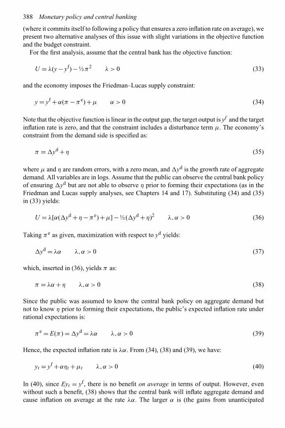
388 Monetary policy and central banking
(where it commits itself to following a policy that ensures a zero inflation rate on average), wepresent two alternative analyses of this issue with slight variations in the objective functionand the budget constraint.
For the first analysis, assume that the central bank has the objective function:
U = λ(y − yf) − ½π2 λ > 0 (33)
and the economy imposes the Friedman–Lucas supply constraint:
y = yf +α(π −πe) +μ α > 0 (34)
Note that the objective function is linear in the output gap, the target output is yf and the targetinflation rate is zero, and that the constraint includes a disturbance term μ. The economy’sconstraint from the demand side is specified as:
π = �yd +η (35)
where μ and η are random errors, with a zero mean, and �yd is the growth rate of aggregatedemand. All variables are in logs. Assume that the public can observe the central bank policyof ensuring �yd but are not able to observe η prior to forming their expectations (as in theFriedman and Lucas supply analyses, see Chapters 14 and 17). Substituting (34) and (35)in (33) yields:
U = λ[α(�yd +η −πe) +μ]− ½(�yd +η)2 λ,α > 0 (36)
Taking πe as given, maximization with respect to yd yields:
�yd = λα λ,α > 0 (37)
which, inserted in (36), yields π as:
π = λα +η λ,α > 0 (38)
Since the public was assumed to know the central bank policy on aggregate demand butnot to know η prior to forming their expectations, the public’s expected inflation rate underrational expectations is:
πe = E(π ) = �yd = λα λ,α > 0 (39)
Hence, the expected inflation rate is λα. From (34), (38) and (39), we have:
yt = yf +αηt +μt λ,α > 0 (40)
In (40), since Eyt = yf, there is no benefit on average in terms of output. However, evenwithout such a benefit, (38) shows that the central bank will inflate aggregate demand andcause inflation on average at the rate λα. The larger α is (the gains from unanticipated
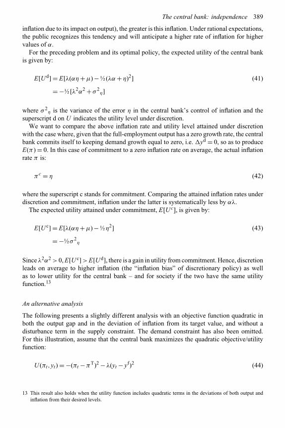
The central bank: independence 389
inflation due to its impact on output), the greater is this inflation. Under rational expectations,the public recognizes this tendency and will anticipate a higher rate of inflation for highervalues of α.
For the preceding problem and its optimal policy, the expected utility of the central bankis given by:
E[U d] = E[λ(αη +μ) − ½(λα +η)2] (41)
= −½ [λ2α2 +σ 2η]
where σ 2η is the variance of the error η in the central bank’s control of inflation and the
superscript d on U indicates the utility level under discretion.We want to compare the above inflation rate and utility level attained under discretion
with the case where, given that the full-employment output has a zero growth rate, the centralbank commits itself to keeping demand growth equal to zero, i.e. �yd = 0, so as to produceE(π ) = 0. In this case of commitment to a zero inflation rate on average, the actual inflationrate π is:
πc = η (42)
where the superscript c stands for commitment. Comparing the attained inflation rates underdiscretion and commitment, inflation under the latter is systematically less by αλ.
The expected utility attained under commitment, E[Uc], is given by:
E[U c] = E[λ(αη +μ) − ½η2] (43)
= −½σ 2η
Since λ2α2 > 0, E[U c]> E[U d], there is a gain in utility from commitment. Hence, discretionleads on average to higher inflation (the “inflation bias” of discretionary policy) as wellas to lower utility for the central bank – and for society if the two have the same utilityfunction.13
An alternative analysis
The following presents a slightly different analysis with an objective function quadratic inboth the output gap and in the deviation of inflation from its target value, and without adisturbance term in the supply constraint. The demand constraint has also been omitted.For this illustration, assume that the central bank maximizes the quadratic objective/utilityfunction:
U (πt,yt) = −(πt −πT)2 −λ(yt − yf)2 (44)
13 This result also holds when the utility function includes quadratic terms in the deviations of both output andinflation from their desired levels.

390 Monetary policy and central banking
where πT is the long-run desired inflation rate.14 Assume, as above, that the central bank’sperceived – and the economy’s actual – aggregate supply relationship is of the Friedman–Lucas (expectations-augmented Phillips curve) type:15
yt = yf +α(πt −πet) α > 0 (45)
For myopic optimization, the expected inflation rate is taken to be given (i.e. it is independentof πt and yt) and the central bank optimizes with respect to πt and yt , taking these given valuesof πe
t. πT and yf to be exogenous to this model. Substituting for yt from (45) in (44) yields:
U (πt,yt) = −(πt −πT)2 −λ(α(πt −πet))
2 (46)
Maximizing this function with respect to πt yields:
πt = (πTt +αλπe
t)/(1 +αλ) (47)
Substituting this value of πt , for given πe, in the objective function (46) yields negativeutility (welfare loss).
If the central bank had followed long-run rather than myopic optimization, it would havehad to treat the expected inflation rate as endogenous. If we assumed the full credibility ofthe central bank’s policy of maintaining inflation at its desired rate, πe
t would equal πTt .
Inserting this in equation (47) yields the long-run result that πt = πTt . Substituting this result
in the supply function yields y equal to yf. Therefore, the objective function (46) yields azero welfare loss. Hence, the failure of the central bank to give an advance commitment toachieving its target inflation rate π∗ for all future periods results in a higher welfare loss thana credible advance commitment. The bank’s mistake in following a myopic policy is that itfails to realize that it can shape expectations and the Phillips curve tradeoff between inflationand output by providing a prior commitment to its policy.
Imposition of goals, constraints and incentives on central banks
The discussion so far in this chapter has shown two distinct sources of inflation bias.16
These are:
• Policy pursued under an incorrect version of the economy’s supply and demand constraintor constraints. In this category would fall the use of the Phillips curve, as against the
14 Depending on the structure of the economy, πT is replaced in some such equations by the last period’s inflationrate.
15 Woodford (2007, equation 2.1) offers the following intertemporal version of this constraint as the new Keynesianaggregate supply function:
πt −π∗t = α ln(yt/yf
t ) +βEt (πt+1 −π∗t+1) +μt α > 0,0 < β < 1
where π∗t is the perceived trend of inflation rate in period t.
16 For the open economy, the central bank may choose to have an objective function that has been modified toinclude disutility of a deviation of the exchange rate (or the balance of payments balance) from its desired level,or its variance. With domestic inflation causing depreciation of the exchange rate, the additional term will tendto reduce the inflationary bias of discretionary policy.

The central bank: independence 391
use of the expectations-augmented Phillips curve. This inflation bias would be due to anerror in the central bank’s knowledge of the economy.
• Policy pursued under the expectations-augmented Phillips curve when the central bankdoes not commit itself to ensuring aggregate demand that will maintain zero inflation onaverage and/or does not have full credibility.
The second source of an inflation bias leads to issues of how to induce or ensure that thecentral bank will follow a zero inflation policy. The literature investigates several scenariosfor achieving it. The simplest would be to mandate the central bank to follow such apolicy.17Another possibility is to provide the central banker with a positive incentive forachieving zero inflation or impose a penalty for deviations from it.18A third possibility isto appoint a central banker who is known to be “conservative” in the sense of attachinga sufficiently higher marginal disutility (compared with society) to inflation than to output(i.e. a sufficiently lower value of λ in the preceding utility functions). It is also importantto protect the central banker from public and governmental pressures to pursue monetarypolicies (e.g. financing a fiscal deficit) that will cause inflation. This raises the question of theindependence of the central bank from the government, discussed earlier in this chapter.Since expectations on central bank policies are important, the central bank’s reputationand credibility in maintaining a low inflation policy also become relevant. Walsh (2003)provides additional discussion of the relevant models on these issues. The next section relatesintertemporal optimization and commitment to the credibility of monetary policy.
12.5.2 Credibility and the costs of disinflation under the EAPC
Credibility becomes especially important in a situation where the actual and expected inflationrates have become high but the central bank decides to pursue a disinflationary policy (i.e.one which reduces the inflation rate) for the current and future periods and announces a targetvalue of πT. Under full credibility, which requires π = πT, as the actual inflation rate is cutby contractionary policies, πe adjusts fully and instantly to πT(= π ), so that (π −πe) remainsat zero and output remains at its full-employment level. With zero credibility, πe would notadjust at all, so that as π is decreased below πe output will fall. Intermediate cases of lessthan full credibility but more than zero will also be accompanied by some loss of output.Therefore, less than full credibility imposes a loss of output in a period of disinflation.
To relate the above to historical experience, money supply targeting in the late 1970s and1980s failed to contain inflation to low rates. Among the reasons cited for this failure of thecentral banks of the USA, UK and Canada, one is that monetary targeting was not pursuedvigorously and maintained long enough. Further, the central banks shifted between targets orpursued multiple targets, often overshot their target inflation rate without later reversing theovershoot, and obscured their targets or the reasons for their failure. Added to these was thepublic’s lack of credibility in the central bank’s commitment and/or ability to achieve lowinflation rates. Another reason for this failure of money supply targeting was the increasinginstability of the money demand function, so that the relationship between inflation, output
17 This is rarely done. The European Central Bank, mandated to follow the sole objective of a zero inflation policy,provides a rare example.
18 This would introduce a third term in the objective function, specifying the incentive or penalty. Such a term isusually made quadratic. This discussion is related to proposals for a contract for the central banker.

392 Monetary policy and central banking
and money supply had become unstable. Once this became known in the 1980s, money supplytargeting was replaced by interest rate targeting.
The 1990s started with the attempts of many countries, including the USA, Canada andthe UK, to lower their rates of inflation. However, the public’s previous experience was withthe higher rates of inflation in the 1980s and the general failure of earlier announcements bytheir central banks of a lower inflation target rate. The credibility of such targets was low,with the consequence that the disinflation process resulted in recessions and loss of output.Therefore, a pertinent issue for the then debate on the appropriate disinflation policy becamewhether or not establishing credibility could be beneficial by itself and what losses mightflow from the lack of credibility. The following parts of this section explore these issues.
To illustrate the issue of the credibility of monetary policy in the context of the Friedman–Lucas supply constraint, assume that the economy starts with identical and high actual andexpected rates of inflation, and that the central bank decides to lower the actual rate of inflation.To achieve this, it follows a restrictive monetary policy, and announces its new policy and thelower inflation rate consistent with that policy. One can imagine several scenarios. In the bestof these, the public believes the central bank and immediately lowers its expected inflationrate to the now lower actual inflation rate, so that the economy maintains full employment.But, in an alternative scenario, if the central bank has gone along this route before but not,in the public’s experience, delivered the requisite contractionary monetary policy and theannounced lower rate of inflation, the public would not find the announcement credible andwould not lower its expected inflation rate correspondingly. Consequently, if the centralbank did in fact deliver the lower announced actual rate of inflation, the expected rate wouldexceed the actual one, so that output would fall below the full-employment level. The lackof credibility was the cause of this fall. By extension, greater rather than lesser credibilityof the central bank would mean a lower shortfall in output. This argument is sometimesused to assert that inflation, possibly even hyperinflation,can be eliminated from an economywithout severe reductions in output and employment – provided that the credibility of thecentral bank is first established by the appointment of appropriate central bank governorswith an established and tough reputation for espousing and establishing price stability.
Consequently, the poor credibility of the central bank introduces a lag in the full impact ofmonetary policy on the economy, and requires the implementation of stronger policies thanwould be otherwise necessary in the interim. The extent of the dilution of its impact and theextension of the length of the lag depend on the “extent of credibility” of the central bank’spolicies.
Credibility and gradualist versus cold turkey policies
Starting from a period of high inflation and low credibility, the restoration of credibilitydepends on the vigor with which the anti-inflationary policies are pursued. The usual analyseson this issue rest on the propositions that the expected inflation rate adjusts to the actualinflation rate with a lag, so that π > πe during the disinflation period, and the adjustment lagof πe is shorter the more severe the recession in output accompanying the disinflation.
The two extreme alternative ways of curbing high inflation are “gradualism” and “coldturkey” policies. Gradualism is a policy of relatively slow reduction in money growth andinflation rates in an attempt to keep the disruption to aggregate demand and output to aminimum during the adjustment to the low desired inflation rate. The economy is thereby notforced into a more severe recession or a rate of unemployment much higher than the naturalone, but the inflation rate falls slowly and takes a longer period to reach the target value.

The central bank: independence 393
In the alternative scenario of the cold turkey policy, the money supply growth rate andaggregate demand are cut drastically, causing the economy to go into a more severe recessionand raising unemployment substantially. The inflation rate falls rapidly. Given such a strongjolt to output and inflation, the public also adjusts rapidly its expectation of inflation to thecentral bank’s target.
Of the two types of policies, the cold turkey solution is clearly the more forceful and drasticpolicy and its impact is often more rapid in lowering the expected rate of inflation, as wellas in creating credibility that the lower rates will be maintained. This faster reduction in theexpected inflation rate means a faster reduction in the actual inflation rate and a reduced lagin the impact of the anti-inflationary policy, which in turn translate into an earlier return tofull employment. As against these benefits, the cold turkey policy usually starts by creatinga deeper recession and greater rise in unemployment than a gradualist policy. Countries tendto follow different combinations of these two policies at different times.
On the costs of disinflationary policies, Ball (1993) reports for his sample a 0.8 percentreduction, on average, of output below its trend level for every percentage point reduction ininflation. Further, he finds that the output costs of anti-inflationary policies tend to be larger ifinflation is reduced gradually over a period of time rather than more rapidly. The cost is likelyto be lower if the policy is credible than if it is not credible, and lower under full credibilitythan under merely rational expectations (Brayton and Tinsley, 1996).
12.5.3 Gains from credibility with a target output rate greater than yf
The credibility of the central bank’s announced inflation rate can yield real gains to theeconomy, as we illustrate in the following model. This model certainty and implicitly assumesthat the central bank has the same utility function as society and that it will achieve the inflationrate that it chooses.
Assume that the central bank wants to choose the optimal values of y and π for its utilityfunction UM:
UM = −γπ2 −[y − kyf]2 γ > 0,k > 1 (48)
where the symbols are as defined earlier. (48) specifies a loss in utility from inflation, as wellas from deviations from the central bank’s pre-specified target output kyf, set in this equationas a proportion of the full-employment output yf. The marginal loss in utility from a unitincrease in output deviation has been normalized at unity.
Again, let the economy’s aggregate supply relationship be of the Friedman–Lucas type,which is:
y = yf +α(π −πe) α > 0 (49)
Substituting (49) in (48) gives:
UM = −γπ2 −[(yf +α(π −πe) − kyf]2 γ > 0 (50)
To find the gains from credibility, we compare the following two extreme cases.
A. There is no credibility and the central bank has to assume the public’s expected inflationrate πe as exogenously given.

394 Monetary policy and central banking
For this case, maximize (50) with respect to π for given πe. This yields the central bank’schoice of π as:
π = α
α2 + γ(kyf − yf) + α2
α2 + γπe (51)
so that the central bank sets its optimal inflation policy to be a function of the expectedinflation rate, the full employment output and the target output. Hence, its target inflationrate will vary as these variables change over time. The inflation rate is positively related toboth πe and (k − 1)yf.
Substituting (51) in (49) yields:
y = yf − α2
α2 + γ(1 − k)yf − αγ
α2 + γπe (52)
Hence, actual output will depend on the target factor k and the expected inflation rate. Ifk = 1, y will not equal yf, even if πe = 0. If k = 1 and πe = 0, y = yf. Further, output is lowerfor higher values of πe. Output can differ from its full-employment level but note that, evenif the former is higher (in the given objective function, higher than kyf), there occurs a lossin utility because of the nature of the assumed quadratic objective function.
B. To see the relative gains from full credibility, now assume that the central bank announcesthe per-period rate of inflation that it intends to achieve and the public fully believes it.In this case, πe = π .
For πe = π , (49) implies that:
y = yf (53)
Therefore, there will not be a loss in output from a disinflationary policy or a gain froman inflationary one, so that, even in the short run, there will not be deviations from fullemployment and their implied loss in utility. Further, the economy enforces k = 1.
Note also that, under full credibility, y = yf whether the central bank’s chosen inflationrate is zero or some positive number. Hence, the output gains from full credibility do notrequire a zero inflation rate, as long as it is known and fully credible. However, with πe = π ,y = yf, so that k = 1. The objective function (48) becomes:
UM = −γπ2 −[(yf − kyf]2 γ > 0 (54)
Maximizing (54) with respect to π yields the condition:
∂U/∂π = −2γπ = 0 (55)
which gives the optimal rate of inflation π∗ as zero. Therefore, for the above model, whilethe gains from credibility occur at any inflation rate, the optimal inflation policy under fullcredibility is that of zero inflation. A positive rate of inflation, even though it may be fullycredible and maintain full-employment output, will yield a lower utility than zero inflation.
Comparing the full credibility results (with y = yf) with those of no credibility, the centralbank can produce higher output by having k > 1 and π > πe. But such deviations from yf

The central bank: independence 395
imply a loss in utility. Further, inflation is positive if there is no credibility and zero if thereis, with the former giving lower utility. Hence, full credibility yields higher utility, lowerinflation and smaller deviations in output from the full-employment level.
12.5.4 Analyses of credibility and commitment under supply shocks andrational expectations
For further exposition of the modeling of credibility, we modify and extend the precedingmodel by again bringing in supply shocks and rational expectations. The model used will be:
UM = −γπ2 −[y − (yf + k)]2 γ,k > 0 (56)19
y = yf +α(π −πe) +μ α > 0 (57)
where μ is a random disturbance to aggregate supply. Note that the objective function (56)differs from that in (48): the output target level now enters the utility function through anadditive rather than a proportional factor.20
We investigate three scenarios for this model.
I. The central bank does not guarantee that the actual inflation rate will be zero but doespre-commit itself to the average inflation rate π being zero. The public believes it andbases its expectations on this average rate, so that πe = π = 0.
Incorporating this restriction into (57) yields:
y = yf +απ +μ (58)
The central bank chooses π to maximize (56) subject to (58), which gives:
π = −βμ+βk (59)
y = yf +αβk + (1 −αβ)μ
where β = α/(α2 + γ ). Hence:
y = yf + α2
α2 + γk + γ
α2 + γμ (60)
However, from (59):
Eπ = βk > 0 for k > 0
19 To allow for a divergence of the central bank’s utility function from society’s, one possibility would be to
define the central bank’s objective function as U M = S −γπ2 −[y− (yf +kM)]2, γ , kM > 0, where S is, say, the
remuneration of the governor of the central bank, and society’s utility function as U S = −γπ2 −[y− (yf +kS)]2,
γ , kS > 0. Such divergence can be used to study performance contracts for central banks. If kM = kS, the centralbank has a different output target from society and, therefore, a different “agenda” (Waller, 1995).
20 The only justification for this change in the objective function from (48) is our desire to present some variationin modeling. As an exercise, the student should derive the results for this section from (48).

396 Monetary policy and central banking
The central bank has given a commitment to π = 0. To meet this commitment when β = 0,it will have to make k = 0 or it would be attempting to fool the public and will not be ableto maintain its credibility. We designate the credible version (with k = 0) of this case as (I′).That is:
I′. Case I above with k = 0, so that the target output level is yf.
Note that the requirement of credibility imposes realism on the objectives of the centralbank. For this credible policy, k = 0, so that:
y = yf + γ
α2 + γμ (61)
π = − α
α2 + γμ (62)
Note that for k = 0, only the rational expectation of inflation Eπ is zero, so that the publicmust be taken to accept that actual inflation will vary over time but maintain its expectedvalue as zero. Further, the expectation of output is stabilized at yf , but its actual level willfluctuate with the actual inflation rate.
II. The central bank guarantees that the actual (rather than the average) inflation rate willbe zero. The public believes it and bases its expectations on it, so that πe = π = 0.
Incorporating this expectations formation into (57) yields:
y = yf +μ (63)
This implies that the central bank cannot achieve k > 0. It must, therefore, give up eitherits target of output greater than the full-employment level or its commitment to a zeroinflation rate.
Further, substituting (63) into the objective function (56) gives:
UM = −γπ2 − (μ+ k)2 γ,k > 0
Maximizing this function with respect to π gives:
∂UM/∂π = −2γπ = 0
so that:
π = 0 (64)
Hence, the optimal inflation rate is zero. However, there may be problems in achieving itsince the model includes random supply shocks that are unpredictable and the central bankmay not be able to implement the policies that will counter their impact on the inflation rate.If the central bank can, in fact, achieve this rate, its optimal inflation policy will be consistentwith its commitment to zero inflation.

The central bank: independence 397
III. The central bank takes πe as given for its decisions while the public forms itsexpectations rationally.
For given πe, maximizing (56) with respect to π and subject to (57) yields:
π = β(απe + k −μ) (65)
where β = α/(α2 + γ ). Assuming rational expectations, so that πe = Eπ ,
πe = (α/γ )k (66)
Equations (65) and (66) imply that:
π = α
γk − α
α2 + γμ (67)
Since Eπ = (α/γ )k , Eπ > 0 for k > 0. Therefore, the equilibrium level of output underrational expectations will be:
y = yf + γ
α2 + γμ (68)
where Ey = yf but y differs from yf.We can now compare inflation and output for the three cases. For this comparison, we will
use for (I) not the general case (k ≥ 0) but (I′), which has a credible commitment to zeroaverage inflation (k = 0). Ey is identical among them. The fluctuations in y are also identicalbetween (I′) and (III). A similar set of implications also holds for the inflation rate. This is aninteresting result into the nature of rational expectations. In (I′), there is a pre-commitment toa credible zero inflation on average. In (III), there is no pre-commitment to any particular rateof inflation but the public, because of its rational expectations, knows and bases its expectedrate on the expected value of the inflation rate adopted by the policy maker. Our conclusionsfrom the above analyses are:
• The identity of results between (I′) and (III) shows that rational expectations act as ifthere were a credible pre-commitment to an average inflation rate, so that it replacesthe need for a pre-commitment. As a corollary, to achieve the benefits of zero inflation,the policy maker does not have to give a pre-commitment as long as it sticks with asystematic zero inflation policy.
• A credible policy is more than just informing the public of the intended policy. It hasto be realistic or it will soon cease to be credible. This requirement imposes limitationson the central bank’s objectives, which in (I′) ensured that the target output was thefull-employment output itself, rather than a higher amount.21
21 Boschen and Weise (2003) provide evidence that inflations in the 1960s, 1970s and 1980s in OECD countrieswere often due to policy makers’ short-term pursuit of high real growth rates – and there was evidence of a linkbetween inflation and national elections.

398 Monetary policy and central banking
• Comparing (I′) and (III) with (II), the expected values of both inflation and outputare the same in all cases but their fluctuations differ. Since γ /(α2 + γ ) < 1, outputfluctuates less and inflation more under (I′) and (III) than under (II). Hence, rationalexpectations reduce the variability of output compared with a policy of zero inflationper period.
Finally, some caveats to the above conclusions. Some of the conclusions are specific tothe assumptions of the above models. Note especially two of these assumptions. One, theassumed quadratic objective function attributes negative utility to even positive deviationsof output from its full-employment level.22 Intuitively, one considers higher output to bemore desirable, so that such positive deviations should have been assigned positive utility.Two, the economy’s constraint has been assumed to have the form of the Friedman–Lucas supply function (i.e. the expectations-augmented Phillips curve). This belongs inthe classical paradigm, whereas the supply constraint of the Keynesian paradigm has adifferent form. We will leave this differentiation to questions at the end of this chapterand to Chapter 15.
Brayton and Tinsley (1996) provide some evidence on the benefits of credibility. Theyfind that the costs in terms of output of disinflation are higher under imperfect credibilitythan under full credibility. Further, they are lower under full credibility than under rationalexpectations.
12.6 Does the central bank possess information superiority?
The success of monetary policy, and its resulting credibility, will depend on knowledgeof the structure of the economy and of the future value of output, prices/inflation, etc.,at the time the policy impacts on the economy. These are practical questions. On thelatter, since there are long lags, say of six quarters, in the impact of monetary policy, thecentral bank must be able to forecast accurately enough the values of the relevant variablesthat far in the future. Such forecasts are prone to error. A more limited requirement ofa useful role for the central bank is that it should possess an informational advantageover the public on forecasting at lag lengths relevant to monetary policy. This can resultfrom superior information gathering and its evaluation of the evidence. Some studies havefound evidence that the US Federal Reserve does possess such superiority (Peek et al.,2003).
12.7 Empirical relevance of the preceding analyses
The analyses of this chapter have assumed special forms of the central bank’s objectivefunctions and the constraints on choices imposed by the economy. Neither of thesemay be valid for any economy or all economies. While the accuracy of the objectivefunction is more difficult to judge from convincing empirical evidence, the empirical
22 This utility function is more in tune with the classical paradigm since it makes the desirable target of monetarypolicy the full-employment level rather than some higher level. A Keynesian might prefer a utility function thatallocates positive utility to positive deviations from full employment.

The central bank: independence 399
estimation of the constraints is quite common. In particular, the aggregate supply equationused in much of this chapter has been the Friedman–Lucas supply function in the formof the expectations-augmented Phillips curve. This function does not yield implicationsconsistent with many, or most, of the stylized facts in Chapters 1 and 14 relatingmoney/inflation to output/unemployment. Therefore, though it has been extensively usedin this chapter and in much of the relevant literature, it is quite likely to be inaccurate asa specification of the short-run supply constraint imposed by the economy on the centralbank’s choices. This would affect the validity and value of the implications drawn in thischapter.
However, it does seem that certain policy recommendations can still be maintained. Amongthese are:
• Intertemporal maximization and its conclusions are preferable to myopic maximization.• The Phillips curve is not a sufficiently valid description of the economy’s short-run
supply constraint, so that the policies derived from it would have an inflationary biasand be especially suspect.
• Credibility of the central bank is important to the success of its policies, especiallywhen it wants to reduce inflation. Given the suspect nature of knowledge of the supplyconstraint, what may be important for the credibility of the central bank is likely to bethe maintenance of its objectives over time, rather than of precise policies derived frominaccurate or imprecise constraints.
• Similarly, given the lack of accurate knowledge of the constraints imposed by theeconomy in both the current and future periods, as well on the actual formation ofexpectations, time-consistent policies may in practice turn out not to be superior toreoptimization policies with an unchanged objective function.
However, it is likely that fine details on the extent of the gains from credibility,especially when there is no difference in output and employment, will not hold up whenthe objective function and the specification of the economy’s constraints are modified toother forms. Nor will fine details on the superiority of time-consistent policies relative toreoptimization ones.
Conclusions
Policy makers need to choose among multiple goals and take account of constraints imposedby the economy on their choices. Since the government and the central bank are likelyto possess different preferences among goals and view these constraints differently, thereexists a potential for conflict between the desired goal levels and the appropriate policies tobe pursued. This potential for conflict tends to be greater when the economy is displayinghigh rates of both inflation and unemployment and tends to be low when the economy haslow rates of both these variables. Such conflicts between central banks and governmentswere more evident during the stagflations of the 1970s and 1980s than they have been sincethen, partly because of the realization that there is no long-run benefit from high inflationrates.
Empirical studies have shown that economies with effectively independent central bankstend to have lower rates of inflation. Therefore, economies with low rates of inflation as asocietal objective should maintain the independence of their central banks.

400 Monetary policy and central banking
The time consistency debate has clearly established the superiority of monetary policiesthat are based on intertemporal optimization as against myopic policies (based on one-period optimization at a time), with the latter being either arbitrary or derived fromone-period optimization subject to a short-run Phillips curve. The latter procedure hasan inflationary bias. Currently, it is not advocated by either the modern classical orthe new Keynesian approaches, but was advocated in the 1950s and 1960s by manyKeynesians.
Time-consistent policy paths are superior to reoptimization policies if there are noshifts in preferences or the economy’s responses over time, as might occur if there is achange in the government or the central bank governor/chairman, if there are shifts in theknowledge of the structure of the economy, or if the central bank’s horizon shortens astime passes. Under uncertainty, a time-consistent intertemporal policy path may requireelaborate policy rules to be specified ex ante. In addition, the benefits of time-consistentoptimization over reoptimization are, at best, likely to be small under the more realisticscenario of a horizon that is long and rolling. The reoptimization procedure is likely tobecome preferable if there are previously unanticipated shifts in the economy’s constraints,which are especially likely to occur under uncertainty of the probabilities of futureoutcomes.
Central banks now accept the conclusion that intertemporal optimization yields betterpolicies than myopic optimization subject to a short-run Phillips curve and that thelatter has an inflationary bias. Hence, they accept the essential contribution of the timeconsistency debate that policies should be formulated with an intertemporal objective functionand must take account of the economy’s anticipated responses and of the anticipatedfuture consequences of policies. Central banks also accept the caution emerging fromthis debate against arbitrary changes in monetary policies if there are no significantshifts in knowledge or of the fundamentals of the economy. Beyond these, monetaryauthorities rarely follow time-consistent policies or their implication of the precise spec-ifications of optimal policies for all future periods and their implementation in thoseperiods.
At the practical level, most central banks maintain discretion to change their policies ifthe economy changes in a significant manner, and have reoptimization powers to decide thepolicy actually pursued in each period, with the understanding or legislated requirement thattheir objectives for the economy do not change. This is currently the practice in the USA,Canada and the UK. Further, limits on the current knowledge of the future course of theeconomy, such as that on the unemployment and growth rates, are recognized in a cautiousapproach to monetary policy; central banks usually change the interest rate in small (usually0.25 percent) steps, leaving open the option of reinforcing this step within a few months, notdoing so, or reversing it as the actual state of the economy reveals itself. This is essentiallya continual reoptimization procedure, with an unchanged utility function, rather than a stricttime-consistent one.
However, no matter what policy is pursued, it is important that the central bank shouldmaintain credibility for its policies. Sticking to pre-announced consistent policies enhancesthis credibility and the effectiveness of the policies pursued. Frequent shifts in policy reducethis credibility, reduce the effectiveness of the policies and also introduce longer lags inthe achievement of the central bank’s targets. Credibility requires that the central bank mustpursue realistic objectives. If its goal is price stability and it has so announced it, and it operatesin the context of a classical-type economy, its target output has to be the full-employmentoutput and not a higher one.

The central bank: independence 401
Appendix
Myopic optimal monetary policy without commitment in a new Keynesianframework
This appendix assumes the new Keynesian quadratic objective function and the newKeynesian supply (price/quantity adjustment) equation (rather than the Friedman–Lucas oneused in the body of this chapter) as the relevant constraint from the economy’s structure.For the following analysis, the new Keynesian objective function is taken to be the quadraticintertemporal objective function:
− 12Et
⎧⎨⎩
∞∑j=0
β j(λ(x#
t+j − k)2 +π#2t+j
)⎫⎬⎭ k ≥ 0 (69)
where x# is the output gap (= y − yf), so that the target output level is the full-employmentlevel plus k(i.e. x# = y − (yf + k)) and π# is the inflation gap, defined as the deviationof inflation from its desired target level πT. β is the central bank’s time discount factorand λ is the weight placed by the central bank on the output gap relative to that on theinflation gap.
For myopic (one-period) optimization, the intertemporal optimization problem of thecentral bank can be replaced by maximization in each period of the function:
−1/2[γ (x#t − k)2 +π#2
t]+ Ht K ≥ 0 (70)
subject to the following new Keynesian supply constraint (new Keynesian Phillips curve)for the current (t) period:
πt = αx#t + ht (71)
where:
Ht = − 12Et
⎧⎨⎩
∞∑j=1
β j(γ (x#
t+j − k)2 +π#2t+j
)⎫⎬⎭ k ≥ 0 (72)
and:
ht = βπet+1 + zt (73)
Note that Ht and ht are given from the perspective of myopic optimization. Treating them assuch assumes that expected future output and inflation are independent of the current outputgap and inflation, so that they are also independent of the policies pursued by the centralbank.23 The central bank maximizes:
−1/2γ (x#t − k)2 − 1/2{(αx#
t + ht) −π∗t)}2 + Ht k ≥ 0 (74)
23 This is clearly unrealistic, which contributes to the undesirability of myopic policies.

402 Monetary policy and central banking
Its first-order condition is:
−γ (x#t − k) −α{αx#
t + ht −π∗t} = 0 k ≥ 0 (75)
Substituting πt = αx#t + ht from the constraint (72) for one of the x#
t in (75) yields:
π#t = −γ
α(x#
t − k) (76)24
Hence, the myopic inflation gap rises with k , which is the amount by which the central bankwants to exceed the full-employment output level. At full employment (i.e. x#
t = 0), thecentral bank will obtain a zero inflation rate if it maintains k = 0. Conversely, the centralbank would ensure deflation by a policy of k < 0. Thus, there is a negative tradeoff betweencurrent inflation above its target level and the current output gap, which the central bank canexercise by choosing its desired value of k .
Equation (76) can also be stated in the form of a supply equation as:
x#t = −α
γπ#
t + k (77)
where x#t is the aggregate demand that the central bank has to ensure for the economy. If
π#t > 0 (i.e. inflation is above target), (77) implies that the central bank reduces aggregate
demand, a policy popularized as “leaning against the wind.”γ is the weight placed by the central bank on the output gap relative to that on the inflation
gap. A central bank that assigns a higher cost to inflation will have a lower value of γ , sothat, from (77), it would maintain aggregate demand and output at a lower level and achievea lower inflation rate.
The central bank can use the money supply or the interest rate as its instrument forachieving the aggregate demand x#
t in (77). If it uses the real interest rate, (77) is substitutedin the IS equation to derive the appropriate real interest rate (rt) to be set by the centralbank. This step requires the specification of the actual form of the IS equation, of whichthere are many forms in the literature. However, for all of them, the central bank reducesaggregate demand by raising the real interest rate, so that if π#
t > 0 0 (i.e. inflation is abovetarget) the central bank raises the real interest rate. In perfect markets, the nominal interestrate (Rt) can be deduced from the Fisher equation (Rt = rt + πe
t). Therefore, to reduceaggregate demand, the central bank raises the nominal interest rate sufficiently to raise thereal interest rate.
If the central bank chooses the money supply as its instrument, it must ensure the moneysupply implied by the IS–LM analysis is required for aggregate demand. For this, the valuesof x#
t and Rt are substituted in the money demand equation to derive the required moneysupply. Since there are many forms of the IS and LM equations in the literature, we do notproceed further with such derivations.
24 Note that assuming rational expectations and substituting for x#t from the budget constraint (29) yields:
π#t = γ (αk + zt +βEtπt+1)
α2 + γ
where the terms involving Eπ can be iterated forward and eliminated, leaving the right side with only parameters.However, the assumption of rational expectations in the context of myopic optimization when the future inflationrates are taken to be independent of the current policy seems questionable.
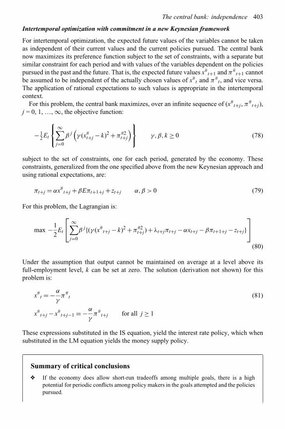
The central bank: independence 403
Intertemporal optimization with commitment in a new Keynesian framework
For intertemporal optimization, the expected future values of the variables cannot be takenas independent of their current values and the current policies pursued. The central banknow maximizes its preference function subject to the set of constraints, with a separate butsimilar constraint for each period and with values of the variables dependent on the policiespursued in the past and the future. That is, the expected future values x#
t+1 and π#t+1 cannot
be assumed to be independent of the actually chosen values of x#t and π#
t , and vice versa.The application of rational expectations to such values is appropriate in the intertemporalcontext.
For this problem, the central bank maximizes, over an infinite sequence of (x#t+j , π#
t+j),j = 0, 1, …, ∞, the objective function:
− 12Et
⎧⎨⎩
∞∑j=0
β j(γ (x#
t+j − k)2 +π#2t+j
)⎫⎬⎭ γ,β,k ≥ 0 (78)
subject to the set of constraints, one for each period, generated by the economy. Theseconstraints, generalized from the one specified above from the new Keynesian approach andusing rational expectations, are:
πt+j = αx#t+j +βEπt+1+j + zt+j α,β > 0 (79)
For this problem, the Lagrangian is:
max −1
2Et
⎡⎣ ∞∑
j=0
β j{(γ (x#t+j − k)2 +π#2
t+j) +λt+jπt+j −αxt+j −βπt+1+j − zt+j}⎤⎦
(80)
Under the assumption that output cannot be maintained on average at a level above itsfull-employment level, k can be set at zero. The solution (derivation not shown) for thisproblem is:
x#t = −α
γπ#
t (81)
x#t+j − x#
t+j−1 = −α
γπ#
t+j for all j ≥ 1
These expressions substituted in the IS equation, yield the interest rate policy, which whensubstituted in the LM equation yields the money supply policy.
Summary of critical conclusions
❖ If the economy does allow short-run tradeoffs among multiple goals, there is a highpotential for periodic conflicts among policy makers in the goals attempted and the policiespursued.

404 Monetary policy and central banking
❖ If the economy does not allow monetary policy to affect output and unemployment evenin the short run – that is, if money is neutral – the adoption of price stability or a lowinflation rate as the single or dominant monetary policy goal becomes more clearly theoptimal policy goal. It also reduces the potential for conflict between monetary and fiscalpolicies.
❖ Central bank independence of the government has been found to reduce the rate of inflation.❖ Time-consistent policies need not be superior to those derived from intertemporal
optimization with an unchanging objective function and a long rolling horizon.❖ Both types of intertemporally optimal monetary policies are superior to myopic policies
and buttress the central bank’s credibility.❖ The credibility of the central bank is essential to its successful reduction of inflation rates.
Credibility is also a factor in reducing the time lags in the adjustment of the expectedinflation rate and of the actual inflation rate.
❖ The credibility of a policy committed to keeping the price level stable imposes a requirementthat the central bank must not try to achieve a target output higher than the full-employmentlevel.
Review and discussion questions
1. Who should determine the economic policy goals for the nation: the governmentdemocratically elected by the public or a central bank whose directors (or governors)are not elected and cannot be made directly responsible to the public? What are some ofthe practices in this respect?
2. It is often argued that independence of the central bank from the government and thelegislature would lead to a lower inflation rate. Why, and under what circumstances isthis likely to happen?
3. The time consistency of policy requires the specification of a policy plan for the future,say for the next five years, and the determination to stick to it. Under what conditions –and shocks – is this a desirable policy? When is it not desirable? Discuss.
4. Show that there can be an inflationary bias in discretionary myopic policies.5. What is the relationship between rational expectations and the credibility of monetary
policy? What do they imply for the relevance of credibility to the success of an anti-inflation program? What do they imply for the choice between a gradualist versus acold-turkey approach to fighting inflation? Discuss.
6. “The time consistency literature suggests that it is always a good thing to have a toughcentral banker who cares about inflation and not at all about unemployment – even ifsociety cares mainly about unemployment.” Discuss.
7. “For pre-specified goals, it is easy for the academic economist to prescribe the course ofmonetary policy for the period ahead. But the devil is in the details: the limitations onthe knowledge of the future course of the economy and its future response to policies,as well as in the implementation of the chosen policies. It is such details that make thesuccessful pursuit of policies an art rather than a science.” Discuss.
8. “Each time the central bank changes its discount rate, there always seems to be plentyof criticism from many economists, some claiming that the change is not needed or toomuch while others claim that it is too little. Is this due to the argumentative dispositionof economists as human beings, as the public seems to suspect, or to the nature of theirdiscipline, or are there other reasons?” Discuss.
The central bank: independence 405
9. Present the IS–LM analysis for the case of negative shifts in the vertical aggregate supplycurve when the targets are (i) aggregate demand, (ii) price stability, (iii) output. Comparethe output and interest rate fluctuations under these targets.
10. Assume that the central bank has the utility function:
U = −u2 − 0.5π2
where U is utility, u is unemployment and π is the inflation rate. Assume that theeconomy imposes a constraint in the form of the Phillips curve. Let this be:
u = 5 − 0.1π
Derive the optimal values of u and π . Compare these optimal values with those under acredible pre-commitment to zero inflation.
11. Given the utility function in the preceding question, assume that the economy has anexpectations-augmented Phillips curve such that:
u − un = −0.1(π −πe)
Derive the optimal values of u and π for (a) exogenously given πe, (b) the rationallyexpected value of πe. Compare these optimal values with those under a credible pre-commitment to zero inflation.
12. Suppose that the economy is such that a positive monetary shock reduces unemployment.Assume that the central bank likes a reduction in unemployment but dislikes an increasein inflation. The public forecasts money growth from the government’s optimizationproblem. How are money growth and inflation determined in this context? If you sowish, you can answer this by specifying a model. What would be the implications of acommitment – i.e. a rule – binding the central bank to a future rate of money growth?Should it do so?
13. What advice would you give the central bank of your country on the appropriate monetarypolicy to follow at the present time? Your answer must specify your assessment of thecurrent state of the economy, and the goals and targets you think the central bank shouldfollow and how they agree with or deviate from those being followed by the centralbank. You must present a detailed analysis of the impact of your suggested policy onoutput, inflation and interest rates.
References
Alesina, A., and Summers, L.H. “Central bank independence and macroeconomic performance: somecomparative evidence.” Journal of Money, Credit and Banking, 25, 1993, pp. 151–62.
Ball, L. “How credible is disinflation? The historical evidence.” Federal Reserve Bank of PhiladelphiaBusiness Review, 1993, pp. 17–28.
Ball, L. “Policy rule for open economies.” In J.B. Taylor, ed. Monetary Policy Rules. Chicago:University of Chicago Press, 1999.
Barro, R.J., and Gordon, D.B. “Rules, discretion and reputation in a model of monetary policy.” Journalof Monetary Economics, 12, 1983, pp. 102–21.
Blackburn, K., and Christensen, M. “Monetary policy and policy credibility: theories and evidence.”Journal of Economic Literature, 27, 1989, pp. 1–45.
406 Monetary policy and central banking
Boschen, J.F., and Weise, C.L. “What starts inflation: evidence from the OECD countries.” Journal ofMoney, Credit and Banking, 35, 2003, pp. 323–49.
Brayton, F., and Tinsley, P. “A guide to FRB/US: a macroeconomic model of the United States.”Federal Reserve Board Finance and Economic Discussion Series, 1996–42, 1996.
Clarida, R., Gali, J. and Gertler, M. “The science of monetary policy: a New Keynesian perspective.”Journal of Economic Literature, 37, 1999, pp. 1661–707.
Cukierman, A., Webb, S.B. and Neyapti, B. “Measuring the independence of central banks and itseffects on policy outcomes.” World Bank Research Review, 6, 1993, pp. 353–98.
Eijffinger, S.C.W., and de Hahn, J. The Political Economy of Central Bank Independence. PrincetonNJ: Princeton University, Special Papers in International Economics, 19, 1996.
Fischer, S. “Rules versus discretion in monetary policy.” In B.M. Friedman, and F.H. Hahn, eds,Handbook of Monetary Economics, vol. II. Amsterdam: North-Holland, 1990.
Goodhart, C.A.E. “Central bank independence.” Journal of International and Comparative Economics,3, 1994. Also in his The Central Bank and the Financial System. London: Macmillan, 1995.
Kydland, F.E., and Prescott, E.C. “Rules rather than discretion: the inconsistency of optimal rules.”Journal of Political Economy, 85, 1977, pp. 473–93.
Lucas, R.E., Jr. “Nobel lecture: Monetary neutrality.” Journal of Political Economy, 104, 1996,pp. 661–82.
Mankiw, N.G. “The inexorable and mysterious tradeoff between inflation and unemployment.”Economic Journal, 111, 2001, pp. C45–C61.
Peek, F., Rosengren, E. and Tootell, G. “Does the Federal Reserve possess an exploitable informationadvantage?” Journal of Monetary Economics, 50, 2003, pp. 817–39.
Rotemberg, J., and Woodford, M. “Interest rate rules in an estimated sticky price model.” In J.B. Taylor,ed., Monetary Policy Rules. Chicago: University of Chicago Press, 1999.
Waller, C.J. “Performance contracts for central bankers.” Federal Reserve Bank of St Louis Review,1995, pp. 3–14.
Walsh, C.E. Monetary Theory and Policy, 2nd edn. Cambridge, MA: MIT Press, 2003.Woodford, M. “How important is money in the conduct of monetary policy?” NBER Working Paper
no. 13325, 2007.

Part V
Monetary policy and themacroeconomy


13 The determination of aggregatedemand
This chapter derives the aggregate demand for commodities in the economy from analyses of thecommodity and money markets. Depending on the central bank’s choice of its primary monetaryinstrument, there are two variants of the money market analysis. In one variant, the central bankcontrols the money supply in a manner that makes it exogenous to the economy. In the othervariant, the central bank controls the interest rate in a manner that makes it exogenous to theeconomy. The first variant leads to the IS–LM analysis of aggregate demand. The second oneleads to the IS–IRT analysis of aggregate demand. The selection between these models for aparticular economy depends on the empirical question: does the central bank make the moneysupply or the interest rate exogenous to the economy?
In both models, monetary and fiscal policies are effective in changing aggregate demand.However, the addition of Ricardian equivalence to both models makes aggregate demandinvariant to fiscal policy changes.
Key concepts introduced in this chapter
♦ IS relationship/curve♦ LM relationship/curve♦ IS–LM analysis♦ Interest rate targeting (IRT)♦ Taylor rule♦ IS–IRT analysis♦ Aggregate demand relationship/curve♦ Ricardian equivalence♦ St Louis equation
This chapter sets out the two variants of the model of aggregate demand that serves asthe workhorse of short-run macroeconomic analysis. The first variant is the IS–LM model,which assumes that the central bank exogenously sets the money supply, and the secondvariant is the IS–IRT model, which assumes that the central bank exogenously sets theinterest rate.
The IS–LM and IS–IRT models aggregate the very large number of goods in the economyinto four types: commodities, money, bonds and labor, with an additional good, “foreignexchange,” for the open economy. Of these goods, money is defined as that good which
410 Monetary policy and the macroeconomy
serves as a medium of payments and bonds are defined as “non-monetary financial assets,”so that they include what are known in everyday parlance as bonds, loans and stocks. Themacroeconomic models analyze the markets for these goods and are basically those orientedtowards the study of general fiscal and monetary policies and their implications for aggregateoutput, employment, interest rates and prices in the short run. The short run in this contextis defined as the analytical (not chronological) period during which the capital stock, laborforce and technology are exogenously given by assumption.
The basic short-run macroeconomic model is known as the IS–LM model if the moneysupply, rather than the interest rate, is exogenously set by the central bank. The correspondingmodel when the interest rate, rather than the money supply, is assumed to be exogenously setby the central bank, can be designated as the IS–IRT model. The choice between the IS–LMand IS–IRT models for the determination of aggregate demand for a given economy is nota matter of dogma or school but depends on the answer to the empirical question: which isthe exogenous monetary policy variable and which is the endogenous one? Therefore, beforeproceeding to the selection of one of these models for a given economy, the appropriateprimary operating target of monetary policy used by the central bank needs to be determined.Hence, the model relevant to one economy can differ from that of another economy if theappropriate operating target is different.
Note that the complete short-run macroeconomic model needs both the aggregate demandand aggregate supply function for commodities in order to determine the price level andaggregate output and employment. The determination of aggregate supply is left to Chapter 14for the classical group of models and to Chapter 15 for the Keynesian group.
13.1 Boundaries of the short-run macroeconomic models
The basic orientation of the short-run macroeconomic models is towards a study of the impactof the general fiscal and monetary policies upon aggregate output and the general price level.There is no attempt to examine their impact upon the relative prices of commodities, sothat these models operate as if in a single commodity world. Further, labor is treated as ifit were a homogeneous input. It is also assumed that the existing capital stock is given andthat while the purchase of commodities for additions to the capital stock (i.e. investment)is made, the productive capacity of the stock does not change because of the gestation lagsbetween purchases of equipment and its use for production. We are, therefore, left withonly one variable input, labor, in the production process. The fixity of capital is one of thedistinguishing characteristics of short-run versus growth models.
The open economy has five basic goods: commodities, money, bonds, labor and foreignexchange. A study of their markets and “prices” requires specification of the demand andsupply for each good, and their equilibrium. Their analysis throughout this chapter is oneof comparative statics, focusing on equilibrium states but with some discussion of out-of-equilibrium adjustments.
13.1.1 Definitions of the short-run and long-run in macroeconomics
The short run is that analytical period in which some variables in the model are held fixed.Therefore, depending upon which variable is being held fixed, there can be many differentdesignations of the short run.
In specifying the macroeconomic model to be short run, rather than a long-run model,one of the variables being held constant is the physical capital stock. Investment in physical
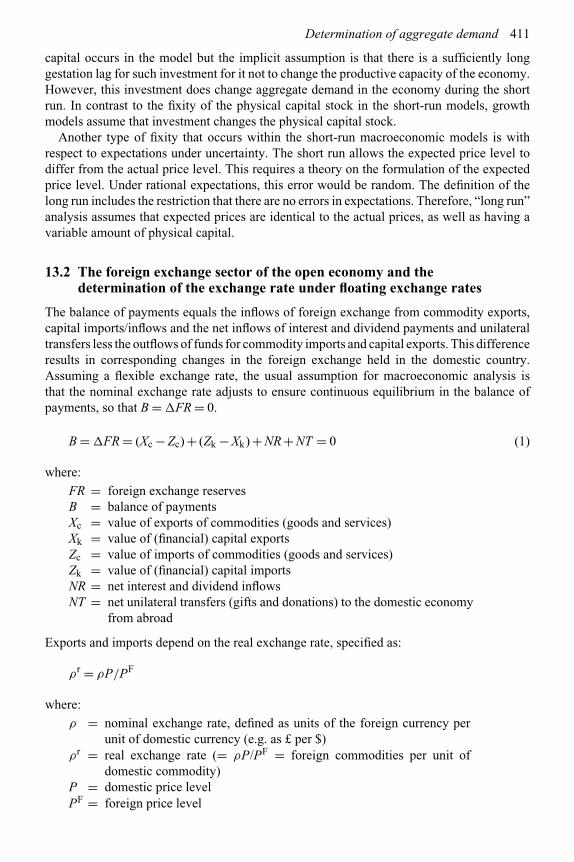
Determination of aggregate demand 411
capital occurs in the model but the implicit assumption is that there is a sufficiently longgestation lag for such investment for it not to change the productive capacity of the economy.However, this investment does change aggregate demand in the economy during the shortrun. In contrast to the fixity of the physical capital stock in the short-run models, growthmodels assume that investment changes the physical capital stock.
Another type of fixity that occurs within the short-run macroeconomic models is withrespect to expectations under uncertainty. The short run allows the expected price level todiffer from the actual price level. This requires a theory on the formulation of the expectedprice level. Under rational expectations, this error would be random. The definition of thelong run includes the restriction that there are no errors in expectations. Therefore, “long run”analysis assumes that expected prices are identical to the actual prices, as well as having avariable amount of physical capital.
13.2 The foreign exchange sector of the open economy and thedetermination of the exchange rate under floating exchange rates
The balance of payments equals the inflows of foreign exchange from commodity exports,capital imports/inflows and the net inflows of interest and dividend payments and unilateraltransfers less the outflows of funds for commodity imports and capital exports. This differenceresults in corresponding changes in the foreign exchange held in the domestic country.Assuming a flexible exchange rate, the usual assumption for macroeconomic analysis isthat the nominal exchange rate adjusts to ensure continuous equilibrium in the balance ofpayments, so that B = �FR = 0.
B = �FR = (Xc − Zc) + (Zk − Xk) + NR + NT = 0 (1)
where:
FR = foreign exchange reservesB = balance of paymentsXc = value of exports of commodities (goods and services)Xk = value of (financial) capital exportsZc = value of imports of commodities (goods and services)Zk = value of (financial) capital importsNR = net interest and dividend inflowsNT = net unilateral transfers (gifts and donations) to the domestic economy
from abroad
Exports and imports depend on the real exchange rate, specified as:
ρr = ρP/PF
where:
ρ = nominal exchange rate, defined as units of the foreign currency perunit of domestic currency (e.g. as £ per $)
ρr = real exchange rate (= ρP/PF = foreign commodities per unit ofdomestic commodity)
P = domestic price levelPF = foreign price level

412 Monetary policy and the macroeconomy
We simplify by assuming that both exports and imports have price elasticities greater thanunity. Therefore, our nominal exports Xc decrease as the real exchange rate ρr (= ρP/PF)rises (which will occur if the domestic price level P rises, ρ rises1 or/and the foreign pricelevel PF falls) since our commodities would become relatively more expensive comparedwith foreign goods. Our exports also increase with an increase in foreign income yF. Similarly,our nominal imports Zc increase if ρr rises (since a unit of our commodities will buymore of foreign ones so that foreign commodities become relatively less expensive) orif domestic income y rises. Capital flows depend upon a range of factors, of which therates of return on domestic and foreign assets are likely to be the most important ones.It will be assumed that capital exports Xk decrease, and capital imports ZK increase, asthe domestic nominal interest rate R rises or the foreign interest rate RF falls.2 Puttingthese ideas formally into (1), the equilibrium condition for the foreign exchange marketbecomes:
[Xc(ρr
−,yF
+) − Zc(ρ
r
+, y+
)]+ [Zk(R+,RF
−,ρ′′e) − Xk(R
−,RF
+,ρ′′e)]+ NR + NT = 0 (2)
where:
y = domestic national incomeyF = foreign national incomeR = domestic nominal interest rateRF = foreign nominal interest rateρ′′e = expected appreciation of the exchange rate
The signs under the variables indicate the signs of the respective derivatives or elasticities.NR (net interest inflows) and NT (net inflows of transfers) tend to be largely exogenous.To the extent that they are not exogenous, their dependence on incomes and interest ratescan be captured in either commodity or capital flows.
We have assumed in the introduction to this chapter that the domestic economy is smallrelative to the rest of the world: that is, the variables PF, yF and RF would not be affectedby changes in our exports and imports of commodities and capital. They are, therefore,exogenous variables whose values are given for our economy. Omitting the variables yF andRF from equation (2) since they are exogenous and omitting ρ′′e for simplification, we areleft with the equation:
[Xc(ρr
−−Zc(ρ
r
+, y+
)]+ [Zk(R+
) − Xk(R−
)]+ NR + NT = 0 (3)
Substituting ρP/PF for ρr in (3) we get:
[Xc(ρP/PF) − Zc(ρP/PF,y)]+ [Zk(R) − Xk(R)]+ NR + NT = 0 (4)
1 Under our definition of the exchange rate, ρ falling (i.e. less £ per $) means that the domestic currency – thedollar – has depreciated, which makes our goods cheaper for foreigners and increases our exports, while makingforeign goods more expensive for us and decreasing our imports.
2 It is also assumed that the other endogenous variables such as incomes, prices and exchange rates are not likelyto significantly affect capital flows from the viewpoint of a purely comparative static analysis.
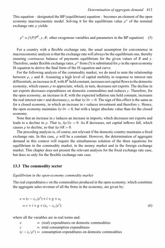
Determination of aggregate demand 413
This equation – designated the BP (equilibrium) equation – becomes an element of the openeconomy macroeconomic model. Solving it for the equilibrium value ρ∗ of the nominalexchange rate ρ yields:
ρ∗ = f (P/PF,y,R; other exogenous variables and parameters in the BP equation) (5)
For a country with a flexible exchange rate, the usual assumption for convenience inmacroeconomic analysis is that the exchange rate will always be the equilibrium one, therebyensuring continuous balance of payments equilibrium for the given values of R and y.Therefore, under flexible exchange rates, ρ∗ from (5) is substituted for ρ in the open economyIS equation to derive the final form of the IS equation and curve.
For the following analysis of the commodity market, we do need to note the relationshipbetween ρ, y and R. Assuming a high level of capital mobility in response to interest ratedifferentials, an increase in R, with RF held constant, increases net capital flows to the domesticeconomy, which causes ρ to appreciate, which, in turn, decreases net exports. The decline innet exports decreases expenditures on domestic commodities and reduces y. Therefore, forthe open economy, an increase in R, with the expected inflation rate held constant, increasesthe real interest rate r and decreases y, so that ∂y/∂r < 0. The sign of this effect is the same asfor a closed economy, in which an increase in r reduces investment and therefore y. Hence,the open economy maintains ∂y/∂r < 0, but with a larger absolute value than for the closedeconomy.
Note that an increase in y induces an increase in imports, which decreases net exports andleads to a decline in ρ. That is, ∂ρ/∂y < 0. As R decreases, net capital inflows fall, whichcauses ρ to decline, so that ∂ρ/∂R > 0.
The preceding analysis is, of course, not relevant if the domestic country maintains a fixedexchange rate. In this case, ρ will be a constant. However, the determination of aggregatedemand in this context will require the simultaneous solution of the three equations forequilibrium in the commodity market, in the money market and in the foreign exchangemarket. This chapter does not present the relevant analysis for the fixed exchange rate case,but does so only for the flexible exchange rate case.
13.3 The commodity sector
Equilibrium in the open-economy commodity market
The real expenditures e on the commodities produced in the open economy, which constitutethe aggregate sales revenue of all the firms in the economy, are given by:
e = (c − zc/ρr) + i + g + xc
= c + i + g + (xc − zc/ρr) (6)
where all the variables are in real terms and:
e = (real) expenditures on domestic commoditiesc = total consumption expenditures(c − zc/ρr) = consumption expenditures on domestic commodities

414 Monetary policy and the macroeconomy
i = (intended) investment3
g = government expenditures on commodities4
zc/ρr = commodity imports (in domestic real terms).
Our exports are already in domestic commodities and are therefore in domestic real terms.zc/ρr(= (PF/ρP)zc) are expenditures in real terms on imported commodities. The reasonfor ρr in the denominator is as follows. zc is the quantity of imported goods bought atforeign prices PF (where F stands for foreign), so that £PFzc (where £ stands for the foreignmoney) is our expenditure in the foreign currency on imported goods. This amount hasto be converted into the domestic currency by dividing by the nominal exchange rate ρ,so that $(PF/ρ)zc is the domestic or dollar price of the imported goods. This nominalamount in dollars has to be deflated into real terms at the domestic price level P to findthe expenditures in domestic real terms on the imported commodities. Therefore, the realvalue of imported commodities in the above equation is not merely zc but (PF/ρP)zc, whichequals zc/ρr.5
In the aggregate over all domestic firms, firms’ output equals their total payments to thefactors of production, which together constitute national income y. National income canbe spent by domestic residents on consumption c (which includes the consumption of bothdomestic and imported goods), on saving s and on payments of net taxes t. Hence,
y = c + s + t (7)
where:
s = (real) private savingt = (real) net taxes paid (net of transfers)
The equilibrium condition for the open economy is:
e = y (8)
In this equilibrium, firms’ revenues e and costs of production y are equal, so that they wouldmaintain production at an unchanged level. But if e > y, firms’ revenues would exceed theircosts and they would be tempted to expand production. If e < y, firms’ revenues would beless than their costs and they would attempt to reduce losses by contracting production.
From (6) to (8), the equilibrium condition for the commodity market can also be stated as:
i + g + xc = s + t + zc/ρr (9)
s = i + (g − t) + (xc − zc/ρr)
Saving is the residual of current output left over after consumption and payment in taxes.This residual may be directly committed for future production in the form of investment,
3 This mode of defining investment excludes “unintended investment,” which mostly consists of commoditiesproduced in the current period and intended for sale but remaining unsold by the end of the period, therebybecoming part of the physical capital stock. The total or accounting measure of investment is the sum of investmentas defined above and unintended investment.
4 Note that government expenditures exclude subsidies and other transfer payments to the public (including firms).5 Some authors do not divide zc by ρr under the assumption that ρr always equals unity or that this is a plausible
enough assumption for the short run. This is done under the implicit assumption that purchasing power parity(PPP) holds, which makes ρr equal to unity. However, PPP does not normally hold, even over periods as long asten or twenty years, let alone periods as short as a month. Therefore, we do not assume that ρr = 1.

Determination of aggregate demand 415
lent to others in exchange for bonds, exchanged for money balances or sent abroad as netexports. Therefore, even in equilibrium, the overall demand for domestic investment goodsis unlikely ever to equal the domestic supply of saving in an open economy in which othergoods, such as bonds, money and foreign goods, exist.
Equilibrium does not always exist in the commodity sector, so that the commodity marketcan have excess demand or supply for some time. Such an excess demand or supply maybe eliminated relatively soon or with a considerable time lag and depends upon the speed ofadjustment towards equilibrium.
13.3.1 Behavioral functions of the commodity market
Further analysis of the commodity market requires specification of the functions for each ofthe variables in the preceding equations. We can proceed further with general forms of thesefunctions or, for simplification, assume linear forms for them. The latter are usually giventhe forms:
c = c(yd ) = c0 + cy(y − t) 0 ≤ cy ≤ 1 (10)
i = i(r) = i0 − irr ir ≥ 0 (11)
t = t0 + tyy 0 ≤ ty ≤ 1 (12)
g = g0 (13)
xc = xc(ρr) = xc0 − xcρρr xc0,xcρ > 0 (14)
zc = xc(yd ,ρr) = zc0 + zcyyd + zcρρr zcy,zcρ > 0 (15)
where r is the real rate of interest and yd (= y − t) is disposable income. Exogenous foreignvariables have been omitted from the equations. Symbols with subscripts are parameters. Wealso have the commodity market equilibrium condition:
e = y (16)
Intertemporal utility maximization subject to the budget constraint implies that consump-tion depends negatively on the real rate of interest, so that (10) should have includedanother term such as −crr on the right-hand side. For the short run, the empiricaldependence of consumption on the rate of interest, for the usual range of interest ratesin the developed economies, is doubtful – and definitely much more doubtful than thedependence of investment on the rate of interest. Further, the impact of such a termwithin the macroeconomic model is identical with that of the dependence of investmenton the rate of interest. Consequently, we have not included the rate of interest in theconsumption function; by implication, the rate of interest will also not be in the savingfunction.6
6 If we believe that saving depends positively on the rate of interest, this can be easily incorporated into the modelby redefining (−ir) to measure the decrease in investment plus the decrease in consumption (or less the increasein saving) induced by the marginal increase in the rate of interest.

416 Monetary policy and the macroeconomy
Note that the preceding equations assume that consumers and firms are free of priceillusion in their consumption and investment decision.7 This assumption is the standard onein macroeconomic models. Further, the preceding consumption and investment functions aresimplified versions of more complicated behavior. In particular, they ignore the dependenceof consumption on consumer confidence and of investment on business confidence,which depend on the expectations of future income, availability of jobs and expecteddemand.
The IS relationship
The preceding equations for the open-economy commodity market imply that:
y =(
1
1 − cy + cyty + 1ρr zcy(1 − ty)
).
[{c0 − cyt0 + i0 − irr + g + xc0 − xcρρr}+ (1/ρr) · {−zc0 + zcyt0 − zcρρr}] (17)8
This equation is the IS equation for the open economy.9 It makes y a function of r and ρr,where ρr = ρP/PF. Replacing ρr by ρP/PF makes y a function of r, ρ, P and PF, in additionto the policy and exogenous variables and parameters. As explained in the preceding sectionon the balance of payments, under flexible exchange rates the equilibrium value ρ∗ of thenominal exchange rate is determined by the balance of payments equilibrium. Replacing ρ
by the determinants of ρ∗ gives the final form of the IS equation. In this equation, y will bea function of P, r, the fiscal policy variables and the exogenous foreign variables PF, rF andyF, but ρ will no longer appear as a separate determinant of y. Since this form is considerablymore cumbersome10 than (17), the standard form of the IS equation, our further analysis ofthe commodity sector will be based on (17) with the understanding that ρr is to be replacedby ρP/PF and ρ is replaced by the determinants of its equilibrium value ρ∗ from the balanceof payments equilibrium condition (4).
However, we do need to derive the sign of ∂y/∂r for the open economy. Under flexibleexchange rates, the earlier balance of payments equilibrium analysis implied that ρ will bea function, among other variables such as P and PF, of the domestic and foreign nominalinterest rates R and RF. Focusing on the relationship between ρ and R, it was shown that anincrease in R, with RF held constant, decreases y. An increase in R, with the expected inflationrate held constant, also increases r. Therefore, for the open economy, ∂y/∂r is negative fortwo reasons: investment is negatively related to r and the increase in r causes an appreciationof ρ and decreases net exports. Hence, the open economy maintains ∂y/∂r < 0, but with alarger absolute value than for the corresponding closed economy.
7 This is not, however, supported by the existing versions of those consumption and investment theories sincethese theories permit substitution between present purchases of commodities for consumption or investment andthose in the future as prices change over time.
8 This is the IS equation without Ricardian equivalence.9 It was given this name since it was originally derived for a closed economy model without a government sector.
Hence, it represented the equilibrium condition i = s.10 In addition, the components of the balance of payments are usually not given commonly accepted simple linear
representations, as is the case of the components of aggregate demand, so that it is difficult to find a linearspecification of the open economy IS equation that embodies the determinants of the equilibrium exchange rate.
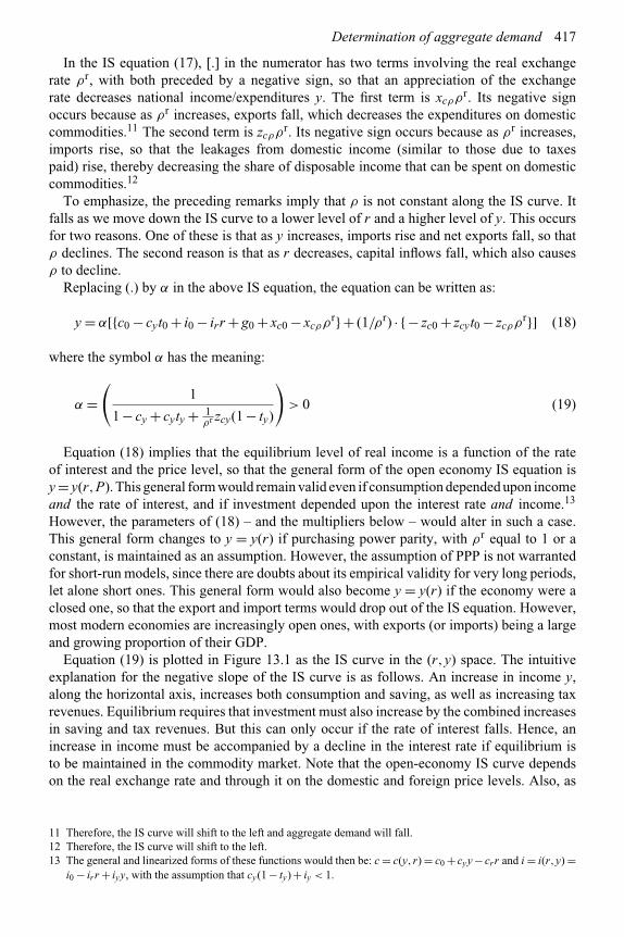
Determination of aggregate demand 417
In the IS equation (17), [.] in the numerator has two terms involving the real exchangerate ρr, with both preceded by a negative sign, so that an appreciation of the exchangerate decreases national income/expenditures y. The first term is xcρρr. Its negative signoccurs because as ρr increases, exports fall, which decreases the expenditures on domesticcommodities.11 The second term is zcρρr. Its negative sign occurs because as ρr increases,imports rise, so that the leakages from domestic income (similar to those due to taxespaid) rise, thereby decreasing the share of disposable income that can be spent on domesticcommodities.12
To emphasize, the preceding remarks imply that ρ is not constant along the IS curve. Itfalls as we move down the IS curve to a lower level of r and a higher level of y. This occursfor two reasons. One of these is that as y increases, imports rise and net exports fall, so thatρ declines. The second reason is that as r decreases, capital inflows fall, which also causesρ to decline.
Replacing (.) by α in the above IS equation, the equation can be written as:
y = α[{c0 − cyt0 + i0 − irr + g0 + xc0 − xcρρr}+ (1/ρr) · {− zc0 + zcyt0 − zcρρr}] (18)
where the symbol α has the meaning:
α =(
1
1 − cy + cyty + 1ρr zcy(1 − ty)
)> 0 (19)
Equation (18) implies that the equilibrium level of real income is a function of the rateof interest and the price level, so that the general form of the open economy IS equation isy = y(r,P). This general form would remain valid even if consumption depended upon incomeand the rate of interest, and if investment depended upon the interest rate and income.13
However, the parameters of (18) – and the multipliers below – would alter in such a case.This general form changes to y = y(r) if purchasing power parity, with ρr equal to 1 or aconstant, is maintained as an assumption. However, the assumption of PPP is not warrantedfor short-run models, since there are doubts about its empirical validity for very long periods,let alone short ones. This general form would also become y = y(r) if the economy were aclosed one, so that the export and import terms would drop out of the IS equation. However,most modern economies are increasingly open ones, with exports (or imports) being a largeand growing proportion of their GDP.
Equation (19) is plotted in Figure 13.1 as the IS curve in the (r,y) space. The intuitiveexplanation for the negative slope of the IS curve is as follows. An increase in income y,along the horizontal axis, increases both consumption and saving, as well as increasing taxrevenues. Equilibrium requires that investment must also increase by the combined increasesin saving and tax revenues. But this can only occur if the rate of interest falls. Hence, anincrease in income must be accompanied by a decline in the interest rate if equilibrium isto be maintained in the commodity market. Note that the open-economy IS curve dependson the real exchange rate and through it on the domestic and foreign price levels. Also, as
11 Therefore, the IS curve will shift to the left and aggregate demand will fall.12 Therefore, the IS curve will shift to the left.13 The general and linearized forms of these functions would then be: c = c(y,r) = c0 + cyy − crr and i = i(r,y) =
i0 − irr + iyy, with the assumption that cy(1 − ty) + iy < 1.

418 Monetary policy and the macroeconomy
y
r
IS
LM
yd
Figure 13.1
shown earlier, the nominal exchange rate ρ declines as the economy moves down the IScurve. But an increase in the domestic price level makes domestic commodities relativelymore expensive than foreign ones and decreases net exports, so that expenditures on domesticcommodities fall and the IS curve shifts to the left for any given interest rate.
The commodity market (partial) multipliers
From the preceding IS equation, some of the various multipliers are:
∂y
∂i0= α =
(1
1 − cy + cyty + 1ρr zcy(1 − ty)
)> 0 (20)
∂y
∂g0= α =
(1
1 − cy + cyty + 1ρr zcy(1 − ty)
)> 0 (21)
∂y
∂t0= (−cy + 1
ρrzcy)α =
( −cy + 1ρr zcy
1 − cy + cyty + 1ρr zcy(1 − ty)
)< 0 (22)
Note that these investment and fiscal multipliers are deceptive and even erroneous for amonetary economy. They are based on the commodity market, which is a very limited part ofthe economy, and ignore the monetary sector, which is also needed for determining aggregatedemand in the economy. Further, they ignore the supply side of the economy. The appropriatemultipliers for the economy are those derived after a general analysis of all the sectors of thewhole economy. Therefore, the usefulness of the above multipliers lies only in studying thedeterminants of the shifts of the IS curve.
13.4 The monetary sector: determining the appropriate operatingtarget of monetary policy
The specification of the monetary sector for any given economy requires the priordetermination of the primary monetary instrument used by its central bank. BenjaminFriedman (1990) provides an extensive discussion of the various instruments and targets of
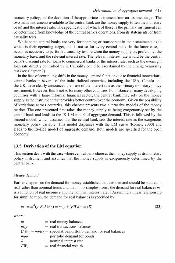
Determination of aggregate demand 419
monetary policy, and the deviation of the appropriate instrument from an assumed target. Thetwo main instruments available to the central bank are the money supply (often the monetarybase) and the interest rate. The specification of which of these is the primary instrument canbe determined from knowledge of the central bank’s operations, from its statements, or fromcausality tests.
While some central banks are very forthcoming or transparent in their statements as towhich is their operating target, this is not so for every central bank. In the latter case, itbecomes necessary to perform a causality test between the money supply or, preferably, themonetary base, and the relevant interest rate. The relevant interest rate would be the centralbank’s discount rate for loans to commercial banks or the interest rate, such as the overnightloan rate directly controlled by it. Causality could be ascertained by the Granger-causalitytest (see Chapter 7).
In the face of continuing shifts in the money demand function due to financial innovations,central banks in several of the industrialized countries, including the USA, Canada andthe UK, have clearly announced their use of the interest rate as the primary monetary policyinstrument. However, this is not so for many other countries. For instance, in many developingcountries with a large informal financial sector, the central bank may rely on the moneysupply as the instrument that provides better control over the economy. Given the possibilityof variations across countries, this chapter presents two alternative models of the moneymarket. The one presented first takes the money supply as being exogenously set by thecentral bank and leads to the IS–LM model of aggregate demand. This is followed by thesecond model, which assumes that the central bank sets the interest rate as the exogenousmonetary policy variable. This model dispenses with the LM curve (Romer, 2000) andleads to the IS–IRT model of aggregate demand. Both models are specified for the openeconomy.
13.5 Derivation of the LM equation
This section deals with the case where central bank chooses the money supply as its monetarypolicy instrument and assumes that the money supply is exogenously determined by thecentral bank.
Money demand
Earlier chapters on the demand for money established that this demand should be studied inreal rather than nominal terms and that, in its simplest form, the demand for real balances md
is a function of real income y and the nominal interest rate r. Assuming a linear relationshipfor simplification, the demand for real balances is specified by:
md = md(y,R,FW 0) = myy + (FW 0 − mRR) (23)
where:
m = real money balancesmyy = real transactions balances(FW 0 − mRR) = speculative/portfolio demand for real balancesmRR = portfolio demand for bondsR = nominal interest rateFW0 = real financial wealth

420 Monetary policy and the macroeconomy
The dependence of money demand on the rate of interest arises from several sources,such as the transactions demand (Chapter 4), the speculative demand (Chapter 5) and theprecautionary and buffer stock demand (Chapter 6). However, for historical reasons relatedto Keynes’s treatment of money demand, the term (FW0 − mRR) is often referred to as thespeculative demand for money.14 We will mostly refer to it as the interest-sensitive moneydemand.
The examination of the money supply process showed that the supply function for moneyshould be specified in nominal terms and that, if the central bank allowed the economyto determine it, it would include the interest rate and real income among its arguments.Alternatively, the central bank could set its level exogenously and achieve it through itscontrol over the reserve base. In line with the latter assumption, we simplify the moneysupply function to:
M s = M (24)
where M is the exogenously determined money stock.Equilibrium in the monetary sector requires that
M = Pmd (25)
Hence, the equilibrium condition in terms of real balances is:
M/P = myy + (FW 0 − mRR) (26)
Equation (26) specifies those combinations of y and R that maintain equilibrium in themonetary market. It is called the LM relationship, where L stands for liquidity preference(i.e. the demand for money) and M stands for the money supply. Note that while the nominalstock of money is exogenously given and in the control of the central bank, the real value ofthat stock, M d/P, depends upon the equilibrium price level P in the economy and incorporateschoices made by the public, including those on its demand for money.
The LM relationship can also be rewritten as:
y = 1
my
[M
P
]+ mR
myR − FW0
my(27)
where 1/my is the real balances multiplier; an increase in real balances by one unit increasesreal income by 1/my.
Equation (27) is plotted in Figure 13.1 as the LM curve. Since ∂y/∂R > 0 in (27), the LMcurve has a positive slope. The intuitive explanation for this slope is: an increase in y alongthe horizontal axis increases the transactions component of the demand for money, requiringthe public to reduce its speculative component mRR, which the public will do only at a higherrate of interest. That is, an increase in real income must be accompanied by an increase inthe rate of interest for equilibrium to be preserved in the monetary sector.
14 Note that the money demand function is often simplified to md = myy − mRR. However, as noted in the text,whether the money demand function is written in this form or as in (23), the interest-sensitive element can alsoarise from the transactions demand analysis presented in Chapter 4. This is especially important since Chapter 5has argued that the modern economy with a variety of riskless assets might not have a positive demand forspeculative balances.

Determination of aggregate demand 421
13.5.1 The link between the IS and LM equations: the Fisher equationon interest rates
The Fisher equation for interest rates asserts that in perfect capital markets, the nominal andreal interest rates are related by the equation:
(1 + R) = (1 + r)(1 +πe) (28)
where R is the nominal interest rate and r the real one. πe is the expected rate of inflation.Assuming low values of re and πe, reπe → 0, so that the preceding equation becomes:
re = R −πe
That is, the real rate that the investor expects to receive equals the nominal rate minus theexpected loss of the purchasing power of money balances through inflation. Comparativestatic analysis with a given money supply does not include the determination of πe so that,for simplification, it can be set at zero or treated as being exogenously determined. Therefore,for simplification, the following analysis assumes that R = r. Alternatively, if inflation didoccur and needed to be incorporated into the money demand function, we could use thesimple form of the Fisher equation, R = r +πe, to write the money demand function as:
md = md(y,R) = myy + (FW 0 − mR(r +πe))
In this case, the LM equation would become:
y = 1
my
[M
P
]+ mR
my(r +πe) − FW0
my(27′)
We choose to base the further development of our model on (27) rather than on (27′), therebyimplicitly assuming a comparatively static, inflation-free environment.
13.6 Aggregate demand for commodities in the IS–LM model
If one focuses on the expenditure and monetary sectors only, the IS and LM curves in the(y,r) space convey the impression that they are enough to determine real income and the rateof interest. This is again incorrect. What is being determined by these markets and curvesis merely the demand for commodities. This demand has to be set against the supply ofcommodities to determine actual real income or output in the economy and the price levelat which this output will be traded. To proceed along this route, we have to first derive fromthe IS–LM analysis the demand for output as a function of the price level.
To derive the demand yd for commodities as a function of the price level P, combine theIS and LM equations (17) and (27): the procedure is to solve the LM equation (27) for r(or R) in terms of y and P, and substitute this value of r in the IS equation (17). The resultingequation is:
yd =(
1
1−cy +cyty + 1ρr zcy(1−ty)+ir
mymR
)·({
c0−cyt0+i0− irmR
FW0
+ irmr
M
P+g0+xc0−xcρρr
}+ 1
ρr
{−zc0+zcyt0−zcρρr}) (29)

422 Monetary policy and the macroeconomy
P
y
AD
Figure 13.2
Equation (29) specifies the aggregate demand for commodities, which is inversely related tothe price level P. (29) specifies those combinations of (y,P) that simultaneously maintainequilibrium in the expenditure and monetary sectors. Figure 13.2 plots equation (29) in the(y,P) space. Designate this curve as the AD (aggregate demand) curve. It has a negativeslope.
Note that our demand function is for an open economy. Specifying ρr = ρ · P/PF andassuming a flexible exchange rate would make the nominal exchange rate ρ endogenous byvirtue of the balance of payments equilibrium condition, so that it will need to be replaced byits function, which does not have a generally accepted form in macroeconomics. The resultingform of the IS equation would become more complex and would also be one that would begenerally less acceptable than (29). Therefore, we do not proceed with this substitution butproceed with (29), while keeping in mind that ρr = ρ · P/PF.
Investment and fiscal multipliers for aggregate demand
The investment and government expenditures multipliers for real aggregate demand nowbecome:
∂yd
∂i0= ∂yd
∂g0=(
1
1 − cy + cyty + 1ρr zcy(1 − ty) + ir
mymR
)
=(
mR
mR − mRcy + mRcyty + 1ρr mRzcy(1 − ty) + irmy
)(30)
These are smaller than those given by (20) and (21) for the expenditure sector alone. Theintuitive explanation for this change is that a given increase in autonomous investment i0increases income through the multiplier, which increases the transactions demand for money.The decreased supply of money balances left for speculative purposes increases interest rates,which forces a reduction in induced investment irr. Total investment, therefore, rises by lessthan the initial increase in autonomous investment. Note that this multiplier becomes zero ifthere are no money balances that can be released from speculative to transactions purposes,as would be the case if mR were zero. Fiscal policy would then have no effect on aggregatedemand.

Determination of aggregate demand 423
The effectiveness of fiscal policy in increasing aggregate demand thus depends not onlyupon the parameters of the expenditure sector but also upon those of the monetary sectorand the foreign trade sector. In particular, fiscal policy cannot affect aggregate demand whenmR = 0; that is, the demand for money – just as its supply – becomes insensitive to the rateof interest.
Money multiplier for aggregate demand
The money supply multiplier, i.e. the increase in aggregate demand for an increase in thenominal money supply, is given by:
∂yd
∂M=(
1
1 − cy + cyty + 1ρr zcy(1 − ty) + ir
mymR
)ir
mR
1
P
=[
ir
mRP − mRPcy + mRPcyty + 1ρr mRPzcy(1 − ty) + Pirmy
](31)
The money multiplier depends upon the relative magnitudes of ir (the interest sensitivityof investment) and mR (the interest sensitivity of money demand). If mR = 0, the moneymultiplier is simply 1/my and if ir = 0, the real balances multiplier is zero. That is,changes in the money supply cannot affect aggregate demand if investment is insensitiveto the rate of interest, i.e. ir = 0, or if the interest rate cannot be changed by monetarypolicy, which occurs in the liquidity trap, i.e. if mR → ∞. In the latter case, any increasein the money supply is absorbed by the infinitely elastic demand for money at theexisting interest rate. This case of an infinitely elastic demand for money at the existinginterest rate is that of the liquidity trap. Following Keynes (1936) and the argumentson this concept in Chapter 2 of this book, we take the view that, while the liquiditytrap is of intellectual curiosity from an analytical standpoint as a limiting case,15 ithas no practical relevance and can be ignored for analyses of the actual functioning ofeconomies.16
Outside the unlikely limits of zero for the money multiplier, the actual magnitude of thismultiplier is of little significance since, given the size of the multiplier, any desired changein aggregate demand can be produced by an appropriate change in the money supply, wherethere is virtually zero difference in cost between changes of different magnitudes in the moneysupply; i.e. within the usual range of operations, a somewhat larger open market operationdoes not cost more than a smaller one.
15 This would be so if the interest rate on bonds were zero. Many economists claim that this was roughly soin Japan at times in the last few decades. However, with the return on bonds being zero, the public, withexcess money balances, is likely to invest the excess in real assets, such as housing, or in domestic and foreignstocks, etc., so that, while there may be a liquidity trap vis-à-vis bonds, it is not likely to occur if all assets areincorporated into the analysis – unless all of them have an expected return equal to zero, which rarely, if ever,happens.
16 The earlier treatment of the liquidity trap was in Chapter 2. We note here again the assertion in Keynes (1936),even though his book was written in the midst of the Great Depression, that he did not consider the liquidity trapto have ever existed in practice.
424 Monetary policy and the macroeconomy
13.6.1 Keynesian–neoclassical synthesis on aggregate demandin the IS–LM model
Empirical findings and analytical development during the 1950s and early 1960s on theinterest elasticities of investment and money demand led to the recognition that, for normallyfunctioning industrialized economies, neither ir = 0 nor mR = 0. Further, such an economydoes not have mR → ∞. Consequently, these extreme cases could be discarded for therelevant macroeconomic analysis, so that the analysis became confined to ir < 0, 0 < mR <∞.Acceptance of these results resulted in what came to be known as the “Keynesian–neoclassicalsynthesis” on the determination of aggregate demand. In this synthesis, as is obvious from thepreceding aggregate demand equation, both monetary and fiscal policies can change aggregatedemand in the economy. Note that this assertion is one about aggregate demand, which equalsnominal national income, and not about output, which equals real national income.
The Keynesian–neoclassical synthesis was upset by Barro’s (1974) contribution of theRicardian equivalence theorem, though the majority of the profession continues to believein the above Keynesian–neoclassical determination of aggregate demand rather than in theform resulting from its incorporation of Barro’s Ricardian equivalence theorem.
13.7 Ricardian equivalence17 and the impact of fiscal policyon aggregate demand in the IS–LM model
While the theory of Ricardian equivalence is not directly relevant to the impact of monetarypolicy, it is relevant to the relative impact of monetary versus fiscal policy on nominal incomein the economy. Ricardian equivalence is the proposition that (bond-financed) fiscal deficitsmerely postpone taxation without changing the economy’s aggregate demand in the currentperiod, as well as in the future. In terms of the IS–LM diagram, Ricardian equivalence impliesthat fiscal deficits and surpluses do not shift the IS curve from its position when the budgetis balanced. This runs counter to the analysis of aggregate demand presented so far in thischapter and to its results on the effects of fiscal policy.
Ricardian equivalence rests on the propositions that, in perfect capital markets,
1 The future tax liability18 imposed by a bond-financed deficit equals the amount of thecurrent deficit.19 This liability arises from the future payment of the interest rate on thebonds and the repayment of the principal amount borrowed.
2 The government supplies exactly the goods that the consumers would have bought ontheir own, so that there is perfect substitutability – in both consumption and production –between government-supplied goods and privately demanded goods.20 Consequently,the arguments of the consumer’s utility function are not the privately bought goods butthe sum of the privately bought and the government-provided goods.
17 Although David Ricardo had raised the main idea behind Ricardian equivalence, he rejected its empiricalsignificance. The modern version of this concept is due to Barro’s contributions (Barro, 1974).
18 The tax liability imposed by a bond is defined as the present discounted value of the future interest paymentsand eventually of the principal at maturity, as specified by the bond.
19 The appendix to this chapter establishes this.20 This assumption is usually not transparent in the standard presentations of Ricardian equivalence since they
normally derive the effects of a deficit created through a reduction in taxes. However, deficits do often comeinto being through an increase in government expenditures. The more general analysis of deficits to cover bothpossibilities requires the above assumption.
Determination of aggregate demand 425
3 Consumers are assumed to have infinitely long lives or to possess an intergenerationalutility function encompassing the utility from their own and their descendants’consumption. This intertemporal utility function can be stated as:
U (.) = U ((cp + cg)1, (cp + cg)2, . . ., (cp + cg)n) (32)
where n can be made arbitrarily large to encompass the period by which the debt usedto finance the current deficit is retired and where cp is privately bought consumer goodsand cg is government-provided consumer goods.
4 The individual maximizes the intertemporal utility function, given the assumptionsof perfect foresight and perfect capital markets, subject to his intertemporal budgetconstraint. This intertemporal personal budget constraint has the form:
�t�tcp
t = �t�t(yt − Tt) t = 1, . . .,n (33)
where T is tax payments/revenues and �t is the discount factor (= 1/(1 − r)t−1) forperiod t. (33) is the usual statement that the present discounted value of the privatelybought goods equals the present value of disposable income.
5 The government’s intertemporal budget constraint, under the assumption of a no ponzischeme21 is:
�t�tcg
t = �t�tTt t = 1, . . .,n (34)
Equation (34) assumes that there is no outstanding debt inherited at the beginning of period 1and asserts that the government-provided goods have to be paid for through taxes overtime. This constraint rules out the monetary financing of deficits and indirectly incorporatestheir financing by a new issue of bonds. The implicit assumption that the discount factors areidentical for the private sector in (33) and the government in (34) requires perfect, unregulatedcapital markets – as well as identical risk premiums for the private sector and the government.Defining the deficit in period t as (cg −T )t , since we have not imposed the requirement thatTi = cg
i, for all i, the government can run a deficit or surplus, or neither, in any particularperiod i. If there is a deficit in period i, with cg
i > Ti, it is covered by issuing bonds at themarket rate of interest, so that higher taxes will have to be paid in the future to cover theinterest on the bonds and their redemption in the future.22
Equations (33) and (34) imply that:
�t�t(cp + cg)t = �t�tyt (35)
which does not include government surpluses and deficits as a variable. Note that y is totalincome, not disposable income.
21 A ponzi scheme is one where the borrower does not expect to eventually pay back his loan.22 Given the public’s resentment over high tax rates and the commonly recognized dependence of labor supply and
tax evasion on the marginal tax rate, we need to recognize – and evaluate the validity of – an implicit assumptionon the labor supply function in establishing the Ricardian equivalence hypothesis. This assumption is that thelabor supply over time is determined by the intertemporal maximization, so that the future labor supply is nota function of the future tax rate. Therefore, high current deficits resulting in high future tax rates do not reducethe future’s labor supply.
426 Monetary policy and the macroeconomy
The public’s choice can now be formulated as: find the total consumption (cpt + cg
t) thatmaximizes (32) subject to (35). This will yield the optimal consumption pattern as:
(cp + cg)t∗ = f (�,PDW) t = 1,2, . . .,n (36)
where:
PDW = �t�tyt (37)
and � is the vector of discount factors. Note that PDW is the present discounted value oftotal income y (rather than of disposable income) so that the optimal total consumption levelsdo not include tax revenues, tax rates or government expenditures among their determinants.Assuming an interior solution and the independence of the present discounted value of wealthfrom fiscal variables, if there is an increase (decrease) in the exogenous supply of government-provided goods in t, the private sector will reduce (increase) its own purchases of goods in tby exactly the same amount, leaving (cp + cg)t invariant to government-provided goods cg
t,tax revenues, deficits and the government debt. That is:
∂(cp + cg)t+i
∂xt+j= 0 for all i, j (38)
where x can be government expenditures, tax revenues or deficits. This result is known asRicardian equivalence.23
Ricardian equivalence is usually stated as the proposition that national saving is invariantwith respect to the fiscal deficit. National saving sn, by definition, is:
snt = yt − (cp + cg)t (39)
where (cp + cg)t is invariant to the size of fiscal deficits. Further, if it is also assumed that ashift in supply from the private to the public good or vice versa has no impact on the aggregateoutput y, ∂yt /∂xt = 0. This assumption means that the efficiency of production by public andprivate sector units is identical, which need not always be valid. Therefore:
∂snt+i
∂xt+j= 0 for all i, j (40)
Hence, snt is invariant with respect to fiscal expenditures and deficits. Further, since national
saving is the sum of private and public saving, where the latter equals the government budget
23 We have stated the assumptions and derivation of the Ricardian equivalence theorem somewhat differently fromBarro’s (1974). In his analysis, the consumer has a time-separable utility function:
U (ct , . . .) = u(ct ) +∞∑
i=t+1
β i−tu(ct )
Such a consumer is sometimes referred to as “dynast.” The consumer maximizes this utility function subjectto Wt−1 = R(Wt − ct ] + yt−1 · ct+i is the consumption of the (t + i)th generation (or the (t + i)th period), W iswealth, y is labor income, R is the intergenerational interest rate and β is the personal discount factor.

Determination of aggregate demand 427
surplus, private saving must fall (rise) by the amount of an increase in this surplus (deficit).This is another way of stating Ricardian equivalence.
The appendix to this chapter relates two of the common propositions of Ricardianequivalence to the evolution of the public debt.
Monetary and fiscal policies in the macroeconomic model withRicardian equivalence
To incorporate Ricardian equivalence into the IS-LM(AD) model of this chapter, we need tomodify its consumption function to accord with the Ricardian results. Designating (cp + cg)tby c′
t and dropping the time subscript t as a simplification for short-run comparative staticanalysis, the short-run Ricardian consumption function c′(y) will be:
c′ = c′(y) = c′0 + c′
yy (41)
Note that c′ refers to the total of privately bought and government-provided goods, anddepends on total income rather than merely on disposable income. Further, there is a changein the meanings of the parameters of the consumption function from those in the neoclassicalmodel presented earlier in this chapter. In (41), c′
y = ∂(cp + cg)/∂y, so that c′y is the sum
of the private and government marginal propensities to consume. Aggregate expendituresin the open economy after the integration of government-provided goods into the precedingconsumption function are now specified by:
e = c′ + i + (xc − zc/ρr) (42)
which no longer includes government expenditures, since these are included in (36). Inequilibrium, e = y, so that (41) and (42) modify the open economy IS relationship to:
y = e = c′ + i + (xc − zc/ρr)
y =(
1
1 − c′y + 1
ρr zcy
)· [{c′
0 + i0 − irr + xc0 − xcρρr}+ (1/ρr) · {−zc0 − zcρρr}] (43)
The aggregate demand function for the open economy becomes:
yd =(
1
1 − c′y + 1
ρr zcy + irmymR
)·
((c′
0 + i0 − irmR
FW0 + irmR
M
P+ xc0 − xcρρr) + 1
ρr(−zc0 − zcρρr)
)(44)
Neither (43) nor (44) includes any of the fiscal variables, so that the changes in governmentexpenditures, taxes and deficits will not shift the IS curve in the IS–LM Figures 13.1 or theAD curve in Figure 13.2, and therefore will have no effects on the macro economy. That is,the fiscal variables cannot be used to change aggregate demand and nominal income in theeconomy, so they do not provide a policy tool for macroeconomic stabilization. Note alsothat, under Ricardian equivalence, fiscal policy does not affect the interest rate.

428 Monetary policy and the macroeconomy
Since the equations of the monetary sector in the neoclassical model are not affected byRicardian equivalence, the only policy tool available for changing aggregate demand andnominal income under Ricardian equivalence is monetary policy. Ricardian equivalence,therefore, buttresses the importance of monetary policy in the economy.24 From (44),Ricardian equivalence changes the money supply multiplier ∂yd/∂M to:
∂yd
∂M=(
1
1 − c′y + 1
ρr zcy + irmymR
)· irmR
1
P
=(
ir
mRP − mRPc′y + 1
ρr mRPzcy + Pirmy
)(45)
Empirical validity of the Ricardian equivalence hypothesis
Ricardian equivalence requires some very strong and seemingly unrealistic assumptions, sothat there are serious questions about its validity. Its validity can be judged on the basisof its assumptions, its implications for the impact of fiscal variables, especially deficits, onaggregate demand and its implications for intergenerational saving behavior.
The impact of fiscal variables on aggregate demand can be tested by the St Louis(monetarist) equation. The St Louis school provided in the late 1960s and early 1970s anempirical procedure for estimating the relationship between nominal income and the moneysupply. This was the estimation of a reduced-form equation of the form:
Yt = α0 +�iaiMt−i +�jbjGt−j +�scsZt−s +μt (46)
where:
Y = nominal national incomeM = vector of the past and present nominal values of the appropriate
monetary aggregateG = vector of the past and present values of the fiscal deficitZ = vector of the other independent variablesμ = disturbance term
The appropriate form of the preceding St Louis equation for testing Ricardian equivalencewould use nominal income as the dependent variable. Its earliest estimation was byresearchers at the Federal Reserve Bank of St Louis (Andersen and Jordan, 1968), whofound25 for the USA that the marginal impact of fiscal policy was positive for the firstyear and then turned negative, with a multiplier of only about 0.05 over five quarters.26
24 This is consistent with the pre-Keynesian emphasis on monetary policy and a general neglect of fiscal deficitsas a policy tool.
25 Another of their findings was that the money aggregates had a strong, positive and rapid impact on nominalincome and this impact was more significant than that of fiscal policy. The marginal money-income multiplierwas about 5 over five quarters.
26 Numerous applications of the St Louis equation showed that the empirical findings from it differed amongcountries, periods and definitions of the policy variables. However, the researchers’ basic conclusion that themoney supply changes have a strong short-term impact on the economy remained fairly robust. Their findingof the insignificance of the impact of fiscal policy on aggregate demand was not, in general, confirmed by otherstudies.

Determination of aggregate demand 429
However, subsequent numerous estimations for different countries and different sampleperiods tended to show that deficits did have a significant positive impact on aggregatedemand.
Ricardian equivalence embodies a special form of the intergenerational saving andbequest function, so that its validity can also be tested directly from the data on savingsand bequests. It has been rejected by household panel studies on intergenerational savingand bequest behavior. Among studies that reject it is that of Carroll (2000), who shows thatBarro’s dynastic model of household consumption and intergenerational saving proves to bea poor description of the behavior of the population, especially of its richest members whocontribute the largest proportion of saving in the economy.
13.8 IS–LM model under a Taylor-type rule for the money supply
A feedback monetary policy rule often proposed for the interest rate policy pursued by thecentral bank is the Taylor rule (Taylor, 1993, 1999). If this rule were adapted to the supplyof money to the economy, the money supply rule would be specified by:
M st = M s
0 −λy(yt − yft) −λπ (πt −πT ) λy,λπ > 0 (47)
where M s0 is determined by the long-run money demand for the given values of yf
t and πT.Implicit in the use of such a rule by the central bank is its acceptance that changes in the moneysupply do change aggregate demand and inflation, and quite possibly short-run (real) outputin a predictable manner, so that monetary policy can reduce the output gap and inflationarypressures in the economy.
13.9 Short-run macro model under an interest rate operating target
Taylor rule
Many central banks, especially in financially developed economies, nowadays choose to usethe interest rate, rather than the money supply, as the primary monetary policy instrument,while leaving the money supply endogenous to the economy. Alvarez et al. (2001) summarizethe current consensus on monetary policy as:
The central elements of this consensus [about the conduct of monetary policy] are thatthe instrument of monetary policy ought to be the short-term interest rate, that policyshould be focused on the short-term interest rate, and that inflation can be reduced byincreasing the short-term interest rate.
Alvarez et al. (2001, p. 219).
Few central banks openly admit to following a specific rule, though several empiricalstudies have shown that they act as if they do so. Among these, the use of the interest rateas the operating monetary policy instrument is often espoused in the form of a Taylor rule(Taylor, 1993, 1999), which is:
rTt = r0 +α(yt − y f) +β(πt −πT ) α,β > 0 (48)

430 Monetary policy and the macroeconomy
where rT is the real interest rate target of the central banks for financial markets, y is realoutput, yf is full-employment output, π is the actual inflation rate, πT is the inflation ratedesired by the central bank, and the subscript t refers to period t. πT is called the targetinflation rate. Similarly, yf is the target output level. (yt − yf) is (minus of) the output gap.The Taylor rule is a feedback rule according to which changes in two indicators, inflationand output, of the actual performance of the economy cause the central bank to change itsreal interest rate target, under this feedback rule, the central bank would increase its targetreal interest rate if actual output (or the demand for it) were too high or if inflation weretoo high, relative to their long-run or desired levels. Taylor used α = 0.5 and β = 0.5,without estimating their values. The usual practice now is to specify the Taylor rule withunspecified values for these parameters, and to estimate them for the country and periodbeing studied. Their relative ratio should reflect the country’s central bank’s responses,over the sample period, to the output gap and the deviation of inflation from its desiredlevel.
Since central banks set the nominal rather than the real interest rate, the Taylor rule is alsooften written as:
RTt = πt + r0 +α(yt − yf) +β(πt −πT) α,β > 0 (48′)
which specifies the nominal interest rate R set by the central bank.The objective of the manipulation of the interest rate by the Taylor rule is to engineer
inflation and output back to their target levels and to do so through a gradual adjustmentpattern. By implication, under the Taylor rule, monetary policy is not used to respond toshocks to the macroeconomy that do not affect the output gap and the deviation of inflationfrom its desired level, so that this rule limits the goals of the central bank to the output gapand inflation.
Under the Taylor rule, as is clear from (48′), if π rises above πT the increase in the targetreal rate will require that the nominal rate has to rise more than the inflation rate; if π fallsbelow πT, a cut in the target real rate will require that the nominal rate has to fall more thanthe inflation rate. Such a policy is sometimes depicted as one of “leaning against the wind.’For any given inflation rate, the greater the value of β, the larger will be the change in thereal and nominal rates and the stronger the movement to stabilize the economy at the targetinflation rate.
Implicit in the Taylor rule are the following propositions about the usual links between theinterest rate, output and inflation:
1 An increase in the real interest rate reduces aggregate demand, which reduces inflation,so that the real interest rate and inflation are negatively related.
2 There is a close positive relationship between output and inflation. Given the structure ofmost economies, there is usually a low positive inflation rate (say, πnairu) when outputis at its full-employment level; inflation rises above πnairu as output rises above itsfull-employment level and falls below πnairu as output falls below that level.27
27 In practice, the price level rarely falls. Rather, deficient demand with output somewhat below the full-employmentlevel leads not to falling prices but to a decrease in the inflation rate (Ball, 1994). The extent of the change ininflation depends on many variables such as the output gap, the expected rate of inflation, changes in the cost ofimported commodities, the rate of increase in the money supply, etc.
The superscript “nairu” stands for “non-accelerating inflationary rate of unemployment.”

Determination of aggregate demand 431
The preceding version of the Taylor rule is a contemporaneous one, in which thecurrent interest rate varies with the current output gap and the “inflation gap,” withthe latter defined as (πt − πT). There are at least three other versions of the Taylorrule in the literature. These include a backward-looking (forward-looking) rule in whichthe current interest rate is set on the basis of past (future) values of the output andinflation gaps. A fourth version derives the Taylor rule from the optimization of aloss function of the central bank. These versions are spelled out in Chapter 15 on theKeynesian paradigm since its current variant (the new Keynesian model) incorporates theTaylor rule.
Note that in the long run yt = yf and πt = πT, rTt = r0, so that r0 has to equal the long-run
real interest rate of the economy. Otherwise, the divergence between the real interest rate setby the central bank and the economy’s real interest rate would cause long-run disequilibriumin the financial markets of the economy, with consequences for the markets for commoditiesand labor, so that neither yf nor πT would be achieved.
In terms of empirical evidence, some form28 of the Taylor rule has often done quite well asthe central bank’s explicit or implicit reaction function for developed, free market economies(Sims, 2001).29 To cite just one empirical study, Clarida et al. (1998) estimate the monetarypolicy rules for France, Germany, Italy, Japan, the UK and the USA. Using a forward-looking version of Taylor’s rule, they report that the central banks of Germany, Japan andthe USA can be implicitly taken to have followed inflation targeting and output stabilizationfunctions.30
An issue actively pursued in further research on the Taylor rule has been whether ornot asset prices and exchange rates should be included in this rule. The argument infavor of their inclusion is that shifts in them can change aggregate demand. However,some part of these shifts are often the result of changes in output and inflation, sothat only the impact of their residual shifts on inflation and output would need to beoffset through monetary policy. Doing so yields extended forms of the Taylor rule.Many empirical studies report that using some form of an augmented Taylor rule,such as incorporating changes in wealth or house prices or exchange rates, leads togreater stabilization of the economy. However, none of these extended forms has comeinto general usage in macroeconomic modeling, so we choose not to present them orincorporate them into the analysis of this chapter. The Taylor rule is re-examined inChapter 15.
28 However, the same form may not do well for all countries or for a given country for all periods. Further,the values of the coefficients may also shift over time, e.g. when the leadership of the central bankchanges.
29 Sims points out that, although simple Taylor rules perform quite well, rules that make the change in the interestrate the dependent variable do better than the original Taylor rule where the dependent variable is the level ofthe interest rate.
30 Kahn and Parrish (1998) discuss the inflation targeting frameworks of various countries, including Canada, theUSA and the UK, and present a table summarizing this information.
Judd and Rudebusch (1998) report that reaction functions of the Taylor rule type summarize well keyelements of US monetary policy during the 1970–1997 period. Levin et al. (1999, 2001) evaluate the robustnessof the estimated policy rules to model uncertainty. Their estimates, from US data for five macroeconomic models,show that a simple version of the inflation and output-targeting rule for the US economy performs quite well.Further, responding to an inflation forecast not longer than a year, the rule does better than for forecasts ofinflation further into the future. Wang and Handa (2007) find that the Taylor rule can also be validly applied toChina, a developing country.

432 Monetary policy and the macroeconomy
Integration of the interest rate as the operating monetary targetinto the macroeconomic model
Our desire in the following analysis is to develop a macroeconomic model that has thesimplicity of the IS–LM one and is comparable with it. In the IS–LM model, the centralbank holds the money supply constant. The corresponding assumption for the interestrate as the monetary policy instrument is that the central bank holds the interest rateconstant. Therefore, for the following analysis, we adopt the assumption that the centralbank sets the real interest rate at a fixed level, rT, which we designate as the “targetrate,” and formulate the macroeconomic model under this assumption. This model canbe used to analyze the impact of changes in this interest rate, irrespective of whetherthe changes are made on a discretionary basis or according to a rule such as theTaylor rule.
The assumption made on monetary policy is that the central bank successfully targetsand sets the economy’s real interest rate r at r0. That is, under this simple targetingpolicy,
r = rT0 (49)
Plotting this interest rate in the (r,y) space of the IS diagram, we have a horizontal line atthe target real interest rate. This is shown in Figure 13.3a by the “interest rate target curve”labeled IRT.31
An alternative to the above assumption of a simple fixed interest rate rule is a simplefeedback rule such as:
r = r0 +λyyd +λPP λy,λP > 0 (49′)
(49′) can also be modified to a Taylor-type rule but with targeting of price level, rather thaninflation, as in:
rTt = r0 +α(yt − yf) +β(Pt − PT) α,β > 0 (49′′)
In (49′) and (49′′), an increase in aggregate demand causes the central bank to raise theinterest rate, so that r and yd are positively related, giving the IRT curve a positive slope, asshown by the IRT curves in Figure 13.3b. An increase in P would not shift the IRT curveunder (49) but would shift those in (49′) and (49′′) upward, from IRT0 to IRT1, indicatingan increase in r at any given level of yd.
Note that, as shown later, under interest rate targeting of whatever type, the money supplybecomes endogenous to money demand, which the central bank accommodates by appropriatechanges in the monetary base. Further, under the simple interest rate targeting in (49), theLM curve becomes horizontal at the set interest rate because the central bank supplies moneyperfectly elastically to the economy. However, the horizontal nature of the LM curve in thiscase does not mean that the economy is in the liquidity trap.
31 Note that the IRT curve replaces the usual LM curve, which is based on the assumption that the central banktargets or sets the money supply. The central bank can target either the interest rate or the money supply, butnot both, so that the LM curve is really not appropriate under interest rate targeting.

Determination of aggregate demand 433
IRT
r
y
(a) (b)
r
y
IRT1
y f
IRT0
r0
r1
Figure 13.3
Although we have a choice of interest rate rules for monetary policy, we will proceed withits simplest version, which is given in (49). While some form of the Taylor rule seems todo quite well empirically for depicting central bank behavior on average and in hindsight,in practice, the adjustment of interest rates by the central bank at any given time does nothappen automatically according to a pre-specified rule and involves considerable discretionand hesitation.32 Further, central bank preferences on the weights put on the output andinflation gaps tend to shift over time,33 as they have done in the USA over the past threedecades with the changes in the chairman of the Federal Reserve System (Clarida et al.,2000). Furthermore, even the assessment of the actual output gap and the current and futurecourse of inflation is usually cloudy, to say the least, and often in dispute.34 Hence, it seemspreferable to present the basic benchmark analysis, intended for general understanding ofthe macroeconomy, on the general nature of the monetary policy instrument rather than onone of the numerous specific forms of the Taylor rule. We therefore proceed with (49) andleave it to the interested reader to derive the aggregate demand functions under (49′) and(49′′) – or one of the other forms of the Taylor rule, some more of which are specified inChapter 15.
32 Both these were remarkably obvious for the US Fed in 2007 in the midst of the subprime financial crisis in theUSA. In fact, John Taylor claimed that the Fed had not followed his rule during 2002 and 2006; had it done so,it would have raised interest rates considerably more than it did, which would have prevented the expansion ofmortgages and other loans at very low interest rates to high-risk borrowers, thereby averting the subprime crisisof 2007.
33 In the United States, this shift usually occurs when there is a change in the Chairman of the Fed, as happenedin 2006 with the change from Alan Greenspan to Ben Bernanke. But there can also be smaller shifts when thecomposition of the Federal Open Market Committee changes.
34 For instance, looking at policy formulation in the USA, 2008 was a particularly cloudy year. It started with fairlyclear signals of a weakening economy and strong expectations of one or more interest rate cuts. By mid-year,because of rising energy and food prices, concern arose about possibly rising inflation. However, the assessmentof the latter was in dispute not only between the Fed Chairman and Wall Street analysts, but, reportedly, alsobetween the Fed policymakers and their own staff economists, and among the members of the Federal OpenMarket Committee.
434 Monetary policy and the macroeconomy
13.9.1 Determination of aggregate demand under simple interest rate targeting
The equation for the aggregate demand (AD) for commodities is obtained jointly from theIS equation for the commodity market and the monetary policy equation determining theinterest rate. Our earlier analysis implies the IS equation to be:
yd = α[{c0 − cyt0 + i0 − irr + g + xc0 − xcρρr}+ (1/ρr) · {−zc0 + zcyt0 − zcρρr}] (50)
where:
α =(
1
1 − cy + cyty + 1ρr zcy(1 − ty)
)> 0 (51)
For monetary policy, in order to reduce unnecessary complexity, as discussed above, weassume the simple monetary policy rule:
r = rT0 (52)
Substitution of (52) in (50) yields the AD equation:
yd = α[{c0 − cyt0 + i0 − irrT
0 + g + xc0 − xcρρr}+ (1/ρr) · {−zc0 + zcyt0 − zcρρr}](53)
The exogenous policy variables in this model are the fiscal ones of g, t0 and ty, while themonetary policy one is rT
0. The respective policy multipliers are ∂yd/∂g = α, ∂yd/∂t0 =[(−cy + zcy(1/ρr))α] and ∂yd/∂rT = −irα. Hence, both fiscal and monetary policies areeffective in increasing aggregate demand. The AD equation is almost the same as the ISequation, so that its investment and fiscal multipliers are identical to the ones derived fromthe IS equation alone.35
Diagrammatic derivation of the AD curve
Aggregate demand in an economy for which the central bank sets the interest rate is given bythe intersection of the IS and the IRT curves. In Figure 13.4a, the intersection of these twocurves at the given interest rate determines the level of the aggregate demand for domesticcommodities. This level is shown as yd. Further, at the given interest rate, a rightward shiftof the IS curve because of increases in investment, government expenditures, exports and theother reasons mentioned above, will increase aggregate demand. A cut by the central bankin the interest rate will also increase aggregate demand.36
Note that the assumption that monetary policy targets the interest rate rather than themoney supply implies that the LM curve is omitted from Figure 13.4a, so that it does notplay a direct role in the determination of aggregate demand (Romer, 2000). Consequently,
35 The AD equation and its multipliers would change under a monetary policy rule that makes the interest ratea positive function of yd. Since there is no change in the qualitative results that we use in later analysis, thecalculation of the AD equation and its multipliers for the interest rate specified as a positive function of y hasbeen left to the interested reader.
36 These results would also hold under a Taylor rule that makes the interest rate a positive function of yd.
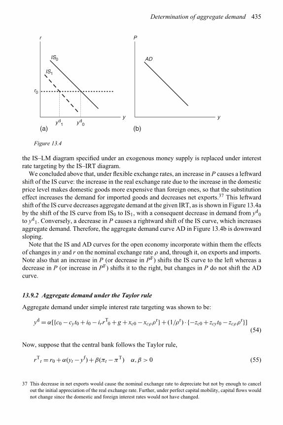
Determination of aggregate demand 435
IS0
r0
IS1
r
yd1 yd
0
y
(a) (b)
P
y
AD
Figure 13.4
the IS–LM diagram specified under an exogenous money supply is replaced under interestrate targeting by the IS–IRT diagram.
We concluded above that, under flexible exchange rates, an increase in P causes a leftwardshift of the IS curve: the increase in the real exchange rate due to the increase in the domesticprice level makes domestic goods more expensive than foreign ones, so that the substitutioneffect increases the demand for imported goods and decreases net exports.37 This leftwardshift of the IS curve decreases aggregate demand at the given IRT, as is shown in Figure 13.4aby the shift of the IS curve from IS0 to IS1, with a consequent decrease in demand from yd
0
to yd1. Conversely, a decrease in P causes a rightward shift of the IS curve, which increases
aggregate demand. Therefore, the aggregate demand curve AD in Figure 13.4b is downwardsloping.
Note that the IS and AD curves for the open economy incorporate within them the effectsof changes in y and r on the nominal exchange rate ρ and, through it, on exports and imports.Note also that an increase in P (or decrease in PF) shifts the IS curve to the left whereas adecrease in P (or increase in PF) shifts it to the right, but changes in P do not shift the ADcurve.
13.9.2 Aggregate demand under the Taylor rule
Aggregate demand under simple interest rate targeting was shown to be:
yd = α[{c0 − cyt0 + i0 − irrT0 + g + xc0 − xcρρr}+ (1/ρr) · {−zc0 + zcyt0 − zcρρr}]
(54)
Now, suppose that the central bank follows the Taylor rule,
rTt = r0 +α(yt − yf) +β(πt −πT) α,β > 0 (55)
37 This decrease in net exports would cause the nominal exchange rate to depreciate but not by enough to cancelout the initial appreciation of the real exchange rate. Further, under perfect capital mobility, capital flows wouldnot change since the domestic and foreign interest rates would not have changed.

436 Monetary policy and the macroeconomy
In this case, the AD equation would become:
yd = α[{c0 − cyt0 + r0 +α(yt − yf) +β(πt −πT) − irrT
0 + g + xc0 − xcρρr}+ (1/ρr) · {−zc0 + zcyt0 − zcρρr}] (56)
which maintains the efficacy of both fiscal and monetary policies in changing aggregatedemand; an increase in fiscal deficits increases aggregate demand, while a rise in the interestrate lowers it.
13.9.3 Aggregate demand under the simple interest rate target andRicardian equivalence
The IS equation under Ricardian equivalence was shown above to be:
y =(
1
1 − c′y + 1
ρr zcy
)· [{c′
0 + i0 − irr + xc0 − xcρρr}+ (1/ρr) · {−zc0 − zcρρr}] (57)
Therefore, the aggregate demand function with Ricardian equivalence and r = rT is:
y =(
1
1 − c′y + 1
ρr zcy
)· [{c′
0 + i0 − irrT + xc0 − xcρρr}+ (1/ρr) · {−zc0 − zcρρr}] (58)
which implies the ineffectiveness of fiscal policies in changing aggregate demand, whilemaintaining the impact of monetary policy on aggregate demand.
13.9.4 The potential for disequilibrium in the financial markets underan interest rate target
Demand for money
The real money demand specified earlier for the 1960s Keynesian–neoclassical synthesis is:
md = md(y,R,FW0) = myy + (FW0 − mRR) 0 < my ≤ 1,0 < mR < ∞ (59)
To cover the possibility that yd (aggregate demand) may not equal ys (aggregate output), wehave to specify whether y in the money demand equation should be yd or ys. Since moneydemand depends upon the planned purchases of commodities, which need to be financedthrough payment in the medium of exchange, money demand would depend on the aggregatedemand for commodities rather on aggregate supply. Therefore, the general money demandequation should be more appropriately specified as:
md = md(yd,R) = myyd + (FW 0 − mRR) 0 < my ≤ 1,0 < mR < ∞ (60)
For perfect capital markets, the Fisher equation on interest rates is:
R = r +πe (61)

Determination of aggregate demand 437
where r is set at rT by the central bank and yd is determined by the AD equation (52) as:
yd = α[{c0 − cyt0 + i0 − irrT
0 + g + xc0 − xcρρr}+ (1/ρr) · {−zc0 + zcyt0 − zcρρr}](62)
Substituting these values of rT and yd in the money demand equation, we get:
md = myα[{c0 − cyt0 + i0 − irrT
0 + g + xc0 − xcρρr}+ (1/ρr) · {−zc0 + zcyt0 − zcρρr}]− mRrT − mrπ
e + FW 0 (63)
Supply of money under interest rate targeting
The money market equilibrium condition is:
M s/P = myα[{c0 − cyt0 + i0 − irrT
0 + g + xc0 − xcρρr}+ (1/ρr) · {−zc0 + zcyt0 − zcρρr}]− mRrT − mRπe + FW 0 (64)
For given P and πe, this equation determines the real money supply M /P required forequilibrium. However, the money market on its own cannot change P, whose movementdepends upon the aggregate demand for commodities relative to their supply. Nor can themoney market change M s (which depends upon the monetary base M0 controlled by thecentral bank) and the monetary base multiplier (∂M /∂M0), which depends on the paymentssystem and public behavior. Therefore, there is no equilibrating mechanism in the moneymarket that will adjust M /P to real money demand, so that unless the central bank providesthe nominal money supply required for money market equilibrium, there is a strong potentialfor disequilibrium in this market.
For the study of dynamic adjustments in disequilibrium, designate the value of M /Pspecified by real money demand as (M/P)d and that specified by the existing nominal moneysupply and price level as (M/P)s. Adopt the plausible hypothesis that if (M/P)d > (M/P)s,the individual members of the public attempt to get additional money balances by sellingbonds, which reduces bond prices, thereby putting upward pressure on the market interestrate. Conversely, if (M/P)d < (M/P)s, the individual members of the public invest theirexcess money holdings by buying bonds, which raises bond prices, thereby putting downwardpressure on the market interest rate.
These movements in the nominal interest rate will produce a deviation of the market-determined interest rate from the target real interest rate plus expected inflation. Thisdiscrepancy will sooner or later produce a sufficient difference and incentive for privatelenders to charge the market-determined rate rather than the central bank’s target rate. Toprevent such a discrepancy, the central bank will need to adjust the monetary base to ensurethat the nominal money supply is suitably adjusted. For our model, it should be specified by:
M s∗ = P[myα{(c0 − cyt0 + i0 − irrT
0 + g + xc0 − xcρρr)
+ (1/ρr) · (−zc0 + zcyt0 − zcρρr)}− mRrT − mRπT + FW 0] (65)
where P is determined by the dynamic adjustments in the commodity market and the termin the [.] specifies real money demand. The star ∗ on M s indicates the endogenous value of

438 Monetary policy and the macroeconomy
the money supply that the central bank needs to achieve if the bond market is to maintain thenominal interest rate at (rT +πe).
Note that (65) replaces the traditional LM equation, but is not really the LM equation, sinceits role now is to endogenously determine the money supply rather than to be an element inthe determination of the price level or of aggregate demand. We will designate it as the M s∗equation, with ∗ standing for money market equilibrium.
The policy problem: providing the money supply neededfor money market equilibrium
Two other considerations need to be added to (65) to determine the money supply that thecentral bank needs to ensure if disequilibrium in the money market at the set interest rateis to be avoided. One, the functions for the variables in (65) will have stochastic terms. Or,alternatively stated, the demand functions for both commodities and money will be stochastic.Two, if there are lags in the system, the appropriate values of the demand for commoditiesand for money will be the expected, rather than the current actual values, for the period whenthe money supply will impact on the economy. These values will involve forecasting errors.In short, it will be difficult for the central bank to predict and provide the money supplyneeded to support its set interest rate in the money market.
If the central bank were to achieve its target inflation rate πT and support its set interestrate, our arguments imply that the money supply would have to be:
M s∗ = P[myα[{c0 − cyt0 + i0 − irrT
0 + g + xc0 − xcρρr}+ (1/ρr) · {−zc0 + zcyt0 − zcρρr}]− mRrT − mRπT + FW 0]+μt (66)
where μt is the stochastic component of money demand. If disequilibrium in the financialmarkets is to be avoided, the actual money supply the central bank would need to provide inperiod t would differ from that specified by (65) by the actual values of μt . The central bankcan provide this money supply through its control of the monetary base exercised throughopen market operations and through changes in reserve requirements or/and by allowingbanks to borrow from it.
The case for allowing borrowing by commercial banks from the central bank
The preceding analysis implies that a central bank that chooses to use the interest rate as itsprimary monetary policy instrument cannot just ignore the money supply.38 Rather, it has toensure an appropriate money supply for equilibrium in the money market. Further, moneydemand may be unstable because of the instability of the IS equation and/or of the moneydemand equation, as has been the case in recent decades. Furthermore, even if money demandis stable, there is likely to be a stochastic element to it. In addition, the central bank doesnot directly control the money supply. Its operative instrument is the monetary base, and themultiplier from the monetary base to the money supply is also likely to be stochastic. Thesefactors individually and collectively cause unpredictability of the appropriate money supply
38 This implies that, even under an interest rate targeting policy, the central bank needs to monitor the monetaryaggregates in the economy. For another view of the benefits from doing so, see Woodford (2007).

Determination of aggregate demand 439
and monetary base. If the central bank is not able to predict and hit its needed amount forequilibrium in the financial markets, it must provide an avenue through which the bankingsystem can, at its own initiative, bring about the required change in the monetary base.Borrowing by commercial banks from the central bank provides such a mechanism and actsas a safety valve against disequilibrium. This role is somewhat distinct from the role of thecentral bank as lender of last resort, which is to guard against a liquidity crisis for individualbanks.
The role of the central bank in accommodating long-term growth in money demand
Since income rises on a long-term basis and inflation increases the price level over time, thereis a secular growth in money demand. This secular growth cannot be accommodated throughborrowing by the commercial banks from the central bank, since such loans are short-termartifacts. Therefore, unless these borrowings are to be allowed to mushroom over time, asthey are never permitted to do, the central bank needs to undertake open market operationsat its own initiative to try and achieve the required monetary base.
Further discussion of changes in the money supply is to be found in Chapter 11 on centralbanking.
13.10 Does interest rate targeting make the money supply redundant?
Interest rate targeting, chosen as the operating target of monetary policy, would make themoney supply redundant if the money supply did not exert an influence on aggregate demandand output independently of the interest rate. Rudebusch and Svensson (2002) find supportfor such redundancy of the money supply. They report, for US data from 1961 to 1996, thatwhile changes in interest rates have a significant effect on output, changes in money do nothave an independent additional influence on output.
However, money supply need not be redundant as an explanatory variable for output, forseveral reasons. Among these, one possibility is that movements in money supply have alagged affect on the long-term interest rate, which affects investment and aggregate demand,so that money supply movements contain information for the future course of output. Anotherexplanation is that changes in the money supply affect the amount and cost of credit, to someextent independently of their impact through interest rates, and the latter have an impact onoutput (see Chapter 16).
Nelson (2002) and Hafer et al. (2007) provide evidence for some independent impact ofthe money supply in explaining output. Hafer and colleagues report, for US data since 1960, astatistically significant impact of money (M2) on output, even after taking account of changesin the real interest rate. Further, movements in both inside and outside money have predictivepower for movements in output. They conclude, therefore, that interest rate targeting doesnot make the money supply redundant in explaining output changes.
Many economies, especially among the LDCs, have fragmented financial markets, withformal and informal financial sectors as well as black (i.e. illegal holdings of) money. In theseeconomies, it is not a priori clear which target of monetary policy would best provide controlover aggregate demand. Offhand, the interest rate seems to be the better instrument forcontrolling the formal financial sector’s impact on commodity demand, while the moneysupply seems to be more effective in controlling the commodity demand fueled by theinformal and black money sectors. Since the two instruments have differential impact onaggregate demand and, especially, on sectoral demands, optimal monetary policy may then
440 Monetary policy and the macroeconomy
pursue the two instruments in LDCs in a less coordinated manner than in financially developedeconomies. In this case, in terms of causation, Granger-causality tests should show two-waycausality between the interest rate and the money supply.
Note that if the money supply does exert an influence on output independent of its impactthrough interest rates, then the interest rate would not be the only useful indicator of the needfor monetary policy, and should not be the only operating target of monetary policy.
13.11 Weaknesses of the IS–LM and IS–IRT analyses ofaggregate demand
The IS–LM and IS–IRT models offer alternative models, depending on the operating targetsof monetary policy, of the determination of aggregate demand for commodities, not thesupply of commodities, output or the price level. The latter are the focus of the next threechapters.
The IS–LM and IS–IRT models suffer from certain weaknesses. Briefly, these are:
1 They do not effectively distinguish between the real interest rate, which determinesinvestment, and the nominal interest rates, which determines the demand for moneyand bonds. From the Fisher equation, the difference between these rates is the expectedinflation rate, the determination of which requires a theory of expectations in addition toa macroeconomic model for determining the inflation rate, which is a dynamic variable.There is no simple way of incorporating these into the IS–LM and IS–IRT models.The simplifying assumption that is then inserted is that the expected inflation rate isexogenous to the model or the model is for comparative static analysis.
2 The IS–LM and IS–IRT models do not recognize more than two distinct financial assets,money and bonds, whereas more than two such assets could enrich the analysis andexplain additional aspects of the macroeconomy. Chapter 16 addresses this concern bydifferentiating credit and loans from bonds.
3 The IS–LM and IS–IRT models are for the short run in which the capital stock, technologyand labor force are held fixed. For certain types of analysis, such as for explainingbusiness cycles and growth, one needs to allow these to vary.
4 The behavioral equations embedded in the standard IS, LM and IRT equations shouldproperly be derived from explicit optimization analysis of rational economic agents, withforward-looking expectations. Some of this analysis is presented in the context of thenew Keynesian IS equation in Chapter 15.
The agenda of macroeconomics in recent decades seems to have been to replace the IS–LMand IS–IRT models by a dynamic stochastic analysis with optimizing agents, who formforward-looking expectations. However, the assumptions adopted to make such modelstractable are such that none has won dominance over the standard IS–LM and IS–IRT modelsas the benchmark models of aggregate demand. In any case, we need to keep in mind whatthese models are meant to do: provide qualitative conclusions on the main determinantsof aggregate demand in a short-run comparative static, not dynamic, context. Admittedly,this is a severely restricted agenda, but it is still a very important one in building one(aggregate demand) of the pillars of macroeconomics. Note that this agenda does not includethe derivation of any qualitative conclusions on the determination of the price level, outputor employment, since any such conclusions would also need the determination of aggregatesupply and equilibrium.

Determination of aggregate demand 441
13.12 Optimal choice of the operating target of monetary policy
The two main operating targets of monetary policy discussed in this chapter have been:
• monetary aggregates;• interest rates.
Chapter 11 used diagrammatic IS–LM analysis to present the central bank’s choice betweenthem if it wants to minimize the fluctuations in aggregate demand, and that chapter shouldbe reviewed as an introduction to the following mathematical one. That analysis and itsfollowing mathematical version were adapted from Poole (1970). Fischer (1990) providesa more extensive discussion and review of the relevant analyses relating instruments totargets of monetary policy. Poole had assumed that the price level was constant. Whilethis was quite a common assumption in the 1960s, it is no longer considered to berealistic or common in modern macroeconomic analysis. Further, taking the price level asconstant, Poole assumed that the central bank’s objective was to minimize the varianceof real output. Since the following analysis does not assume a constant price level andthe central bank can only affect output through aggregate demand and expenditures, itmakes the assumption that the central bank wants to minimize the variance of aggregatedemand.
Using the earlier IS–LM equations for the determination of aggregate demand, the generalstochastic form of the IS and LM equations for the closed economy can be written as:
IS: ydt = −αrrt +μt (67)
LM: (M/P)t = −mRRt + myydt +ηt (68)
where the variables are now defined as deviations from their trend values, so that the constantsin the IS–LM equations have been omitted. The definitions of the symbols are otherwise asgiven earlier in this chapter. μt is the stochastic disturbance to expenditures on commoditiesand ηt is the stochastic disturbance in the money market. μt and ηt are assumed to have a zeromean, be serially uncorrelated and also uncorrelated with each other. They are assumed to beunpredictable and the central bank is assumed to make its decisions prior to observing theiractual values. The right side of (67) specifies expenditures on commodities, with αr capturingthe interest-sensitivity of these expenditures. The right side of (68) specifies money demandin real terms.
This IS–LM model needs to be supplemented by a relationship between rt and Rt . This isprovided, for an economy with perfect capital markets, by the Fisher equation:
Rt = rt +πet (69)
where πet is the expected inflation rate for period t. Holding these expectations constant as a
simplifying analytical assumption, Rt and rt can be treated as identical in the IS–LM model.Hence, replacing Rt by rt in the LM equation, the model becomes:
IS: ydt = −αrrt +μt (70)
LM: (M/P)t = −mRrt + myydt +ηt (71)

442 Monetary policy and the macroeconomy
The central bank observes the values of all terms, except those of the shocks, prior tosetting its policy instrument, which is either Mt or rt . Its objective function is to minimizethe expected variance of aggregate demand around its trend value, i.e.
minimize E(ydt)
2 (72)
Since y has been defined in terms of deviations from its trend, note that the equilibrium valueof yd in the absence of shocks (μ = η = 0) would be zero, so that its variance arises only byvirtue of μ and η being different from zero.
When the money stock is the policy instrument, we need to solve (70) and (71) to deriveyd
t , which is given by:
IS-LM: yd = αrM/P + mRμ−αrη
αrmy + mR(73)
Since Eμ = Eη = 0, E(yd) = (αrM/P)(αrmy+mR) . Hence, noting that the variables in the current
model are being defined in terms of deviations from their trend values, targeting M such thatE(yd
t) = 0 requires M/P = 0, which yields:
yd = mRμ−αrη
αrmy + mR(74)
Therefore, under the assumption that μ and η are uncorrelated and the variance ofαPP is zero, the variance of aggregate demand under the money supply instrument isgiven by:
Em(yd)2 = mR2σμ
2 +αr2ση
2
(αrmy + mR)2(75)
where the superscript m on E indicates monetary targeting.When the real interest rate is the monetary policy instrument, the IS equation (70) alone
needs to be solved for ydt . Under interest rate targeting, setting r such that E(yd
t) = 0, itsvariance becomes:
Er(yd)2 = σμ2 (76)
where the superscript r on E indicates interest rate targeting. Monetary targeting is preferableto interest rate targeting if (75) is less than (76), and vice versa. The former requires:
mR2σμ
2 +αr2ση
2
(αrmy + mR)2< σμ
2 (77)
which simplifies to:
ση2 < σμ
2(
my2 + 2mymR
αr
)(78)
Determination of aggregate demand 443
Hence, if there are only money market shocks but no commodity market shocks (i.e.σμ = 0), then interest rate targeting is preferable since doing so perfectly stabilizesaggregate demand; the LM equation and its disturbance term become irrelevant to thedetermination of aggregate demand. But if there are only commodity market shocks butno money market shocks (i.e. ση = 0), then monetary targeting is preferable since doingso reduces fluctuations in aggregate demand. In this case, with a given money supply, apositive commodity market shock raises the interest rate, which reduces interest-sensitiveexpenditures, thereby reducing commodity demand, so that the original shock to demand ispartially offset.
In the general case, the choice of the policy instrument will depend on the relativemagnitudes of the shocks and the slope of the IS curve (whose slope is −1/αr) relativeto that of the LM curve (whose slope is 1/mr). If, for simplification, the term in parentheseson the right-hand side of (78) were ignored, monetary targeting would be preferable tointerest rate targeting if the stochastic disturbance in the money market were smallerthan in the commodity market. For the money market, assuming that the central bankcan precisely control the money supply but does not know the money demand becauseof the instability of this demand, ση occurs because of the volatility of money demand.For the commodity market, if we were to assume that the instability of commoditydemand arises only because of the instability of investment (though consumption and netexports can also be volatile), σμ occurs because of the volatility of investment demand.These assumptions provide the commonly used, but simplified, statement of the precedingcondition as: monetary targeting is preferable if investment is more volatile than moneydemand, but interest rate targeting is preferable if money demand is more volatile thaninvestment.
The preceding analysis ignores several aspects of the economy. Regarding the moneysupply, the central bank does not directly control the money supply. It controls themonetary base, which provides rather imperfect control over the money supply formost economies. Further, the money supply and money demand functions may beunstable, so that their parameters shift over time, with the shifts being unpredictableat the decision time. Regarding the interest rates, the central bank can set its discountrate and manage the overnight loan rate for reserves, but these need not, dependingon the structure of the financial markets, provide precise control over market ratesor over their differentials. Further, the forms of the IS and LM equations used inthe preceding analysis are fairly simple ones and ignore such elements as expecta-tions and factors, such as the exchange rate and net exports, relevant to the openeconomy.39
Other possible operating targets of monetary policy
In addition to interest rates and monetary aggregate as the operating targets of monetarypolicy, other targets proposed for this purpose include nominal income (or aggregate demand)(see McCallum, 1985; Ireland, 1998) and the price level (see Barro, 1986; Ireland, 1998).The desirability of these targets can be assessed from their welfare effects in the context ofa given welfare objective function of the public or of the central bank.
39 Walsh (2006) explores the effects of variations in the model for determining the optimal policy instrument.

444 Monetary policy and the macroeconomy
Conclusions
The technique of analysis used in this chapter has been one of grouping the relationshipsof the commodity and money market into a single AD equation. This procedure resulted inthe IS-LM model for use when the central bank follows a simple money supply rule and theIS–IRT model when it follows a simple interest rate rule. Which rule is relevant to a giveneconomy? If the money demand function is stable and predictable and the central bank cancontrol the money supply and the interest rate equally well, it does not matter whether thecentral bank follows a simple money supply rule or a simple interest rate rule. But it doesmatter when the money demand function is not stable. In this case, the use of the interest rateas the monetary policy instrument may be preferable.
Ricardian equivalence added to the assumptions of the macroeconomic model impliesthat fiscal policy cannot change aggregate demand. This is so for both the IS–LM andIS–IRT models. With fiscal policy thus made ineffective, monetary policy acquires evenmore importance as the instrument for inducing changes in aggregate demand.
Under interest rate targeting, with the interest rate set exogenously by the central bank, theanalysis of this chapter implies that the financial sector can be omitted from the determinationof aggregate demand and, therefore, from any influence on the economy. However, such animplication is incorrect: to avoid disorderly financial markets, the money supply has to equalthe money demand at the set interest rate. Failure to do so will bring about a different interestrate in the financial markets, with the consequence that the central bank will lose controlover the economy’s interest rates. Another reason for studying the money supply arises if theappropriate macroeconomic model includes bonds and loans as two non-monetary assets,with loans being supplied by the financial sector and with imperfect substitution betweenbonds and loans. The analysis of this case is provided in Chapter 16.
Appendix
The propositions of Ricardian equivalence and the evolution of the public debt
I. Define the amount of outstanding bonds, each with a real value of one unit ofcommodities, at the beginning of period i to be bi, and assume b1 = 0. The bondsissued in period i receive interest in period i+1. The evolution of the value of the publicdebt bi+1 is specified by:
bi+1 =i∑
t=1
φt(cgi−t+1 − Ti−t+1) (79)
where φt is the interest compounding factor (= (1+r)t), which multiplies the past deficitsto arrive at their present value, and r is the real interest rate. (79) specifies the evolutionof the public debt over time under the assumption that there is no default.
To relate Ricardian equivalence to the public debt, we need to incorporate itsassumption that any bonds issued by the government to finance current deficits areredeemed by some future date n which is within the representative individual’s horizon40
40 This horizon can be farther than the representative individual’s expected date of death and will cover the lifetimesof his intended beneficiaries.

Determination of aggregate demand 445
for consumption planning. Since all outstanding government bonds are redeemed at theend of period n, bn+1 = 0. Hence, setting i = n in (79):
bn+1 =n∑
t=1
φt(cgn−t+1 − Tn−t+1) = 0 (80)
so that:
n∑t=1
φtcgn−t+1 =
n∑t=1
φtTn−t+1 (81)
where φt = (1 + r)t . Multiplying both sides of (81) by (1 + r)−n, we get:
n∑t=1
1
(1 + r)n−tcg
n−t+1 =n∑
t=1
1
(1 + r)n−tTn−t+1 (82)
which is the same as:41
n∑t=1
1
(1 + r)t−1cg
t =n∑
t=1
1
(1 + r)t−1Tt (83)
Equation (83) is identical to (34) for the government’s intertemporal budget constraint,assumed earlier in this chapter for the derivation of Ricardian equivalence.
II. If the interest rate paid on bonds and the discount rate are identical, Ricardian equivalenceincorporates the assertion that the present value of the future tax liability42 imposed bythe bonds issued to finance the deficit equals the deficit itself. To show this, let the deficitd be financed by the current issue of bonds b, so that b = d, and designate by PV b thepresent value of the future tax liability. With the payment of the interest Rb at the endof each period and the repayment of the principal P (= b) at the end of period n, PV b isgiven by:
PVb =n∑
t=1
RP
(1 + R)t+ P
(1 + R)n
= P
(n∑
t=1
R
(1 + R)t+ 1
(1 + R)n
)
= P (1) = P (84)43
where R is the nominal interest rate. Since P = b = d, PVb = d, so that the present valueof the future tax liabilities from a bond-financed deficit equals the deficit itself.
41 To see this, write out the preceding equation in its long form (without the summation sign).42 That is, the interest payments prior to redemption and the payment of the principal on the redemption of the
bonds.43 If we let D = 1/(1 + R), the proof uses the mathematical formula:
n∑t=1
Dt =n∑
t=0
Dt − 1 = 1 − Dn+1
1 − D− 1

446 Monetary policy and the macroeconomy
Summary of critical conclusions
❖ Under certainty, or with a stable and predictable money demand function, it does not matterwhether the central bank chooses the money supply or the interest rate as its operatingmonetary policy target. Under uncertainty and stochastic functions, it does matter.
❖ For an economy for which it can be validly assumed that the money supply is the monetarypolicy instrument and is exogenously determined by the central bank, the appropriate modelof aggregate demand is the IS–LM model.
❖ For an economy for which it can be validly assumed that the interest rate is the monetarypolicy instrument and is exogenously determined by the central bank, the appropriate modelof aggregate demand is the IS–IRT model.
❖ The addition of Ricardian equivalence to both models makes aggregate demand invariantto fiscal policy, but does not qualitatively affect the scope and impact of monetarypolicy.
Review and discussion questions
1. For a small open economy with a floating exchange rate whose movements continuouslyensure equilibrium in the balance of payments, draw the locus of points in the IS–LMdiagram (with the interest rate on the vertical axis and real income on the horizontalone) at which equilibrium exists in the foreign exchange market. In this diagram, do wealso need to draw a BP curve (designating the balance of payments equilibrium points)in addition to the IS and LM curves for aggregate demand analysis? Discuss why orwhy not.
2. It is often asserted that there is a national income identity, so that in a closed economywithout a government sector there is an identity between saving and investment. Explorethe implications of this statement by doing the following:
Given a closed economy without a government sector, modify the IS–LM model by theassumption that saving and investment are identical (i.e. equal under all circumstancesand not merely in equilibrium) and answer the following: What is the level of aggregatedemand? Is the LM relationship required for its determination? Is any interest rateconsistent with equilibrium in the commodity market?
Now discuss the following statements: “For purposes of a satisfactory theory of moneysupply and prices, the IS relationship must never be treated as an identity, so that there isonly a national income equilibrium condition.” “A satisfactory macroeconomic modelmust incorporate the potential for disequilibrium between saving and investment, evenin a closed economy without a government sector.”
3. Suppose that the government wants to increase its expenditure g and has the options offinancing it by higher taxes, bond issues or increases in the monetary base. Further, wheng is increased through bond or monetary financing, the central bank can also undertakeoffsetting open market operations. What combinations, if any, of financing methodsand open market operations will allow the following goals to be met in the IS–LMmodel:
(i) no change in aggregate demand;(ii) no change in investment;(iii) no change in aggregate demand and investment?
Determination of aggregate demand 447
4. Present the analysis of the statement that the effects of government deficits on aggregatedemand depend on the way in which the deficit is financed.
Also, analyze the above statement for the following cases:
(i) the central bank is known to follow the rule of stabilizing the growth of the moneysupply;
(ii) government debt (bonds) is only sold to the central bank;(iii) the central bank is known to follow the rule of stabilizing the nominal rate of
interest.
5. The central bank has decided to adopt one of the following money supply rules:
(a) M s = kPy(b) M s = ky
where k > 0. Show their implications for aggregate demand in the context of (i) theIS–LM model and (ii) the IS–LM model with a zero speculative demand for money (i.e.mR = 0). Is each of these policies viable?
6. One of the banking innovations in the 1960s was the payment of interest on certain typesof demand deposits. Assume that interest is paid on money at the rate Rm, which equals(R-x), where x is exogenously determined in nominal terms by market structures and thecost of servicing deposits.
(i) Use the Baumol–Tobin transactions demand model to derive the demand functionfor money.
(ii) Generalizing the above demand function to md(y,R,x), show the behavior of theLM curve for shifts in x and P.
(iii) What is the effect of an increase in x on aggregate demand and the price level in theIS–LM model?
(iv) Assuming that both r and x always increase by the expected rate of inflation, carryout (ii) and (iii) again.
7. “In a closed economy, if the money stock is held constant by the central bank, an increasein the government deficit does not have either short-run or long-run effects on aggregatedemand or the interest rate.” Discuss in the context of the IS–LM model and the IS–LMmodel with Ricardian equivalence.
8. Modify the general IS–LM model of this chapter to the appropriate model for aclosed economy. Specify the IS, LM and aggregate demand equations. What causesthe dependence of aggregate demand on the price level?
9. Assuming that the central bank follows a simple interest rate target rule, modify thegeneral IS–IRT model of this chapter to the appropriate one for a closed economy.Specify its IS and aggregate demand equations. Is the price level P a variable inthese equations? Plot the IS and AD equations and discuss the reasons for theirslopes.
10. Assuming that the central bank follows a simple interest rate target rule, write an essayon the determination of the money supply that would maintain equilibrium in the moneyand bond markets. Discuss how the central bank can ensure this money supply if themoney demand function is unstable and unpredictable.
11. Can monetary and fiscal policies be independent of each other? If not, why is theirindependence postulated in the IS–LM and IS–IRT analyses? Discuss.

448 Monetary policy and the macroeconomy
12. The “crowding out” hypothesis is the statement that fiscal deficits reduce investment; inthe limit, full crowding out means a reduction in investment equal to the fiscal deficit.Is crowding out fully or partially valid in the IS–LM and IS–IRT models? Can completecrowding out occur in the context of (a) a financially advanced economy, (b) a financiallyunder-developed economy?
13. What are the ways or reasons under which fiscal deficits can crowd out privateexpenditures in the determination of aggregate demand? In this discussion, do not forgetthe Ricardian equivalence theorem.
14. In the IS–LM model, discuss how each of the following affect the relative efficacy ofmonetary and fiscal policies:
(a) the interest elasticity of money demand;(b) the interest elasticity of investment;(c) the income elasticity of money demand.
15. “It makes no difference whether government expenditures are financed by taxes orbonds.” Specify a theoretical basis for this statement. Provide at least two reasons whyit may not hold.
16. Discuss the rationale and validity of the following statements: “It makes no differencewhether government expenditures are financed by money or bonds.” “A fiscal deficit hasa larger impact on aggregate demand if it is financed by money than if it is financed bybonds.”
17. An empirical study tested for the Ricardian equivalence theorem by estimating thefollowing equation:
�At = a0 + a1�Bt +μt
where A is the public’s net real financial assets (excluding its holdings of governmentbonds), B is real public debt and μ is a random term. Does a1 = 1 confirm the Ricardianequivalence theorem? US aggregate time series tend to yield a1 = 0. What would thisimply for the validity of the Ricardian equivalence theorem?
Formulate and specify at least one other estimation equation for testing the Ricardianequivalence theorem.
18. Assume that the IS and money demand equations each have a disturbance term. Further,assume that the central bank can control the economy’s interest rate r and money supplyM s except for uncontrollable disturbance terms ηt and νt , so that:
r = rT +ηt
M s = M + νt
Use Poole’s analysis to derive the conditions for preferring interest rate targeting overmoney supply targeting, and vice versa.
Assume that the central bank chooses to target the interest rate in the precedingequation. Derive the money supply that the central bank needs to ensure for equilibriumin the money market. What would happen if it did not ensure this money supply?Discuss.
19. In the preceding question, suppose the central bank uses open market operations to aimat the money supply. Discuss the case for it to allow borrowing from it by commercial

Determination of aggregate demand 449
banks at the latter’s initiative. Is the argument for such borrowing different from thatusually offered for the lender-of-last-resort function of central banks? Discuss.
References
Alvarez, F., Lucas, Jr. R.E. and Weber, W.E. “Interest rates and inflation.” American Economic Review,91, 2001, pp. 219–25.
Anderson, L.C., and Jordan, J.L. “Monetary and fiscal actions: a test of their relative importance ineconomic stabilization.” Federal Reserve Bank of St. Louis Review, 1968, pp. 11–24.
Ball, L.B. “What determines the sacrifice ratio?” In N.G. Mankiw, ed., Monetary Policy. Chicago:University of Chicago Press, 1994.
Barro, R.J. “Are government bonds net wealth?” Journal of Political Economy, 82, 1974,pp. 1095–118.
Barro, R.J. “Recent developments in the theory of rules versus discretion.” Economic Journal, 96,1986, pp. 23–7.
Carroll, C.D. “Why do the rich save so much?” Chapter 14 in J.B. Slimrod, ed., Does Atlas Shrug?Cambridge, MA: Harvard University Press, 2000.
Clarida, R., Galí, J. and Gertler, M. “Monetary policy rules in practise: some international evidence.”European Economic Review, 1998, 42, pp. 1033–67.
Clarida, R., Galí, J. and Gertler, M. “Monetary policy rules and macroeconomic stability: evidence andsome theory.” Quarterly Journal of Economics, 115, 2000, pp. 147–80.
Fischer, S. “Rules versus discretion in monetary policy.” In B.M. Friedman and F.H. Hahn,eds, Handbook of Monetary Economics, vol. II. Amsterdam: North-Holland, 1990, Ch. 21,pp. 1155–84.
Friedman, B.M. “Targets and instruments of monetary policy. “In B.M. Friedman and F.H. Hahn, eds,Handbook of Monetary Economics, vol. II. Amsterdam: North-Holland, 1990, Ch. 22, pp. 1185–230.
Hafer, R.W., Haslag, J.H. and Jones, G. “On money and output: Is money redundant?” Journal ofMonetary Economics, 54, 2007, pp. 945–54.
Ireland, P.N. “Alternative nominal anchors.” Canadian Journal of Economics, 31, 1998, pp. 365–84.Judd, J.P. and Rudebusch, G. “Taylor’s rule and the Fed: 1970–1997.” Federal Reserve Bank of
San Francisco Economic Review, 1998, 3, pp. 3–16.Kahn, G.A. and Parrish, K. “Conducting monetary policy with inflation targets.” Federal Reserve Bank
of Kansas City Economic Review, 1998, pp. 5–32.Keynes, J.M. The General Theory of Employment, Interest and Money. New York: Macmillan, 1936.Levin, A., Wieland, V. and Williams, J.C. “Robustness of simple monetary policy rules under model
uncertainty.” In J.B. Taylor, ed., Monetary Policy Rules. Chicago: Chicago University Press, 1999,pp. 263–99.
Levin, A., Wieland, V. and Williams, J.C. “The performance of forecast-based monetary policyrules under model uncertainty.” Board of Governors of the Federal Reserve System, WorkingPaper 2001–39, 2001.
McCallum, B.T. “On consequences and criticisms of monetary targeting.” Journal of Money, Credit,and Banking, 17, 1985, pp. 570–97.
Nelson, E. “Direct effects of base money on aggregate demand: theory and evidence.” Journal ofMonetary Economics, 49, 2002, pp. 687–708.
Poole, W. “Optimal choice of monetary policy instruments in a simple stochastic macro model.”Quarterly Journal of Economics, 84, 1970, pp. 197–216.
Romer, D. “Keynesian macroeconomics without the LM curve.” Journal of Economic Perspectives,14, 2000, pp. 149–69.
Rudebusch, G.D. and Svensson, L.E.O. “Eurosystem monetary targeting: lessons from US data.”European Economic Review, 46, 2002, pp. 417–42.
Sims, C.A. “A review of monetary policy rules.” Journal of Economic Literature, 39, 2001,pp. 562–6.

450 Monetary policy and the macroeconomy
Taylor, J.B. “Discretion versus policy rules in practise.” Carnegie–Rochester Conference Series onPublic Policy, 39, 1993, pp. 195–214.
Taylor, J.B. Monetary Policy Rules. Chicago: Chicago University Press, 1999.Walsh, C.E. Monetary Theory and Policy. Cambridge, MA: MIT Press, 2006.Wang, S. and Handa, J. “Monetary policy rules under a fixed exchange rate regime: empirical evidence
from China.” Applied Financial Economics, 17, 2007, pp. 941–50.Woodford, M. “How important is money in the conduct of monetary policy?” NBER Working Paper
No. 13325, 2007.

14 The classical paradigm inmacroeconomics
The most enduring tradition in short-run macroeconomics is represented by the classicalparadigm. This chapter covers the various schools and models of this paradigm. Themicroeconomic foundations of the classical paradigm lie in the Walrasian model, presentedin Chapter 3 above. In long-run equilibrium, the models of the classical paradigm imply fullemployment and full-employment output in the economy, and money neutrality, so that thereis no need for the pursuit of fiscal or monetary policies to improve on the already perfectfunctioning of the economy. In short-run equilibrium, deviations from full employment occurdue to errors in price or inflationary expectations. These deviations and the resulting departuresfrom the neutrality of money are transient and self-correcting.
The chapter starts with the stylized facts on the relationship between money, inflation andoutput. To be valid and useful, macroeconomic theories need to be able to explain these facts.
Key concepts introduced in this chapter
♦ The neoclassical model♦ The employment–output relationship/curve♦ The long-run aggregate supply relationship/curve♦ The short-run aggregate supply relationship/curve♦ The natural rate of unemployment♦ Economic liberalism♦ Laissez faire♦ The Great Depression♦ Monetarism♦ The traditional classical approach/theory♦ The modern classical model/theory♦ The new classical model♦ Real business cycle theory♦ Notional versus effective demand and supply functions♦ Ricardian equivalence♦ Pigou and real balance effects♦ Rational expectations♦ Expectations-augmented Phillips curve♦ Friedman and Lucas supply rules

452 Monetary policy and the macroeconomy
Chapter 1 presented a brief definition of the classical paradigm and its component models.Chapter 2 covered the heritage of monetary and macroeconomic theory, and in Chapter 3we presented microeconomic analyses of the demand and supply functions for commodities,money and labor. These chapters should be reviewed at this stage.
Chapter 13, on the determination of aggregate demand, is a prerequisite for this chapter,which takes the determination of aggregate demand as a given for its analysis.
As was pointed out in Chapter 1, there are two major paradigms in short-run macromodeling: classical and Keynesian. The classical paradigm encompasses the traditionalclassical set of ideas, the neoclassical model, the modern classical model and the new classicalmodel. This chapter starts with the neoclassical model and returns to the other two modelstowards the end.
As in earlier chapters, lower case symbols will generally refer to the real values of thevariables and upper case symbols to their nominal values.
Stylized facts on money, prices and output
Monetary macroeconomics is vitally concerned with the empirical relationships betweenmonetary policy, prices, inflation and output. For a macroeconomic theory to be valid anduseful, it must do a reasonable job of explaining these relationships. The stylized facts onthese relationships are:
1 Over long periods of time, there is a roughly one-to-one relationship between the moneysupply and inflation (McCandless and Weber, 1995).
2 Over long periods, the relationship between inflation and output growth is not significantor, if significant, is not robust (Taylor, 1996).1 This is also so for money growth andoutput growth (Lucas, 1996; Kormendi and Meguire, 1984; Geweke, 1986; Wong, 2000),though some studies show a positive correlation between these variables, especially forlow-inflation countries (McCandless and Weber, 1995; Bullard and Keating, 1995),while others show a negative relationship (Barro, 1996).
3 Over long periods of time, the correlation between money growth rates and nominalinterest rates is very high (about 0.7 or higher) (Mishkin, 1992; Monnet and Weber,2001), so that changes in interest rates tend to reflect changes in inflation.
4 In the short run, changes in money supply and interest rates have a strong impact onaggregate demand (Anderson and Jordan, 1968; Sims, 1972).
5 Changes in money growth lead to changes in real output in business cycles (Friedman andSchwartz, 1963a, b). Unanticipated money supply changes affect output (Barro, 1977),as do anticipated ones (Mishkin, 1982) (see Chapter 9). Negative shocks to money supplyhave a stronger impact on output than positive ones (Cover, 1992).
6 Monetary policy increases (decreases) in the short-term interest rate lead to a decline(an increase) in output (Eichenbaum, 1992).
7 On monetary policy dynamics in the short run, monetary shocks build to a peak impacton output and then gradually die out, so that there is a “hump-shaped pattern” of theeffect of monetary policy on output (see Mosser (1992), Nelson (1998) and Christianoet al. (1999) for evidence on the United States, and Sims (1992) for evidence for some
1 In relation to this proposition, Taylor (1996, p. 186) concludes that “there is now little disagreement … that thereis no long-run trade-off between the rate of inflation and the rate of unemployment.”

The classical paradigm 453
other countries) with the peak effect occurring with a lag longer than one year, sometimestwo to three years.
8 As a corollary of the preceding point, the impact of monetary shocks on prices occurswith a longer lag than on output, so that the impact of monetary shocks on output doesnot mainly occur through prior price movements.
9 For the short run, since inflation responds more gradually than output to monetary policychanges, expected inflation also responds more gradually. Therefore, errors in price orinflation expectations do not provide a satisfactory explanation of the response of outputto monetary policy shifts.
10 Unanticipated price movements explain only a small part of output variability. Theimpact of unanticipated, as well as anticipated, monetary shifts on real output do notnecessarily occur through prior price/inflation increases (Lucas, 1996, p. 679).
11 The responses of output and prices to monetary shocks differ over different episodes.They are also stronger for contractionary than for expansionary monetary episodes.
12 Contractionary monetary policies to reduce inflation do initially reduce output signifi-cantly (Ball, 1993), often for more than a year. The cost in terms of output tends to belarger if inflation is brought down gradually rather than rapidly. It is lower if the policyhas greater credibility (Brayton and Tinsley, 1996).
14.1 Definitions of the short run and the long run
Equilibrium in a model is defined as that state in which all markets clear, so that the demandand supply in each market are equal. Another definition is that it is the state from which thereis no inherent tendency to change. The classical paradigm uses the former definition. Thelatter definition is met when the former one is satisfied.
The long run of the short-run macroeconomic model is defined as that analytical periodin which:
1 There are no adjustment costs, inertia, contracts or rigidities, so that all adjustments tothe desired or equilibrium values of its variables are instantaneous.
2 There are no errors in expectations, so that the expected values of the variables areidentical with their actual values. This condition is trivially satisfied if there is certainty.
3 There exists long-run equilibrium in all markets.
Note that these assumptions imply that there are no labor contracts between firms andworkers and no price contracts among firms, so that prices and nominal and real wagesadjust instantly and fully to reflect market forces. However, the long run of the short-runmacroeconomic model still assumes that the capital stock, labor force and technology areconstant.
Given these assumptions, the economy’s resulting long-run employment level is said to bethe “full-employment” level and its long-run output is said to be “full-employment output,”for which our symbol is yf. Note that the long-run – or full-employment – output is not reallythe maximum output that the economy could produce at any time, e.g. if all its resources wereused 24 hours a day. It is also not the equilibrium level of output that would be producedin the short run or the actual output that might be produced when the economy is not inequilibrium. Hence, macroeconomics interprets the term “fully employed” in a special way.It is formally defined as being the level of output and employment that would exist in long-runequilibrium of the short-run macroeconomic model. Intuitively, this corresponds to the levels
454 Monetary policy and the macroeconomy
of output and employment that can be sustained by the economy over the long run with itscurrent supplies of the factors of production and its current technology – given its currenteconomic, political and social structures, as well as the wishes of the owners of the factorsof production.
By comparison with the definition of the long run, the short run in the context of theshort-run macroeconomic model is defined as that analytical period in which:
1 Some variables, especially the capital stock, technology and labor force, are constant.2 There can be adjustment costs, e.g. of adjusting prices, wages, employment and output
to their desired levels, as well as inertia, contracts or/and rigidities of some kind.3 There can be errors in expectations; e.g. the expected values of variables such as prices,
inflation, wages and aggregate demand, differ from their actual values.4 There can be disequilibrium in any or all of the markets.5 The short-run equilibrium values of the various variables can differ from their long-run
values. In particular, the short-run output can be greater or less than its full-employmentlevel.
The actual values of the variables in the economy can differ from their long run andshort-run equilibrium levels for a variety of reasons. This would occur if the actual economyis not even in short-run equilibrium or suffers short-run deviations from full employmentdue to factors other than errors in price expectations. Note that actual output occurs in achronological time period whereas the short run and the long run are analytical, hypothetical,constructs. Illustrating this point by reference to the output of commodities, there are threeconcepts of output: actual output, short-run equilibrium output and long-run equilibrium(full-employment) output.
Also, note that the terms “short run” and “long run” are different in meaning from theircounterparts of “short period” or “short term” and “long period” or “long term.” The formerare analytical constructs indicative of the forces allowed to work in the analysis; the latterare chronological ones and refer to an interval of actual time. In the real world, the economicforces encompassed in both the analytical short run and the long run operate simultaneouslyat every moment of time in the economy. To illustrate, the population and the capital stock arecontinuously changing, so that the analytical forces of the long-run growth models must becontinuously operating in the economy, even over the next day, month or quarter.2 At the sametime, the analytical forces of the short-run macroeconomic models are also simultaneouslyoperating in the economy.
14.2 Long-run supply side of the neoclassical model
Production function
In industrialized, as against agricultural, economies, capital and labor are the dominantinputs in production, while land plays only a minor role and is normally not included inmacroeconomic analysis. With this assumption, the production of commodities is taken to
2 Note that Keynes’s famous remark that “in the long run we are all dead” is not valid under the above interpretationof the long run.

The classical paradigm 455
use only labor and capital as inputs. The production function for the economy – as representedby that for the representative firm – can then be written as:
y = y(n,K) yn,yK > 0;ynn,yKK < 0 (1)
where:y = outputK = physical capital stockn = labor employed.
The physical stock of capital has already been assumed to be constant in the short-runmacroeconomic context of our analysis, so that K = K , where the underlining indicates“constancy” or “exogeneity,” as required by the definition of the short run. Hence, we have:
y = y(n,K) yn > 0,ynn < 0 (2)
With this modification, labor is left as the only variable input, with a positive relationshipbetween output and employment. The assumption of yn > 0 and ynn < 0 is that the marginalproductivity of labor is positive but diminishing: successive increments of labor yield smallerand smaller increments of output.
Labor market in the long run
The specification of the labor market requires specification of the demand and supplyfunctions of labor and its equilibrium condition. Their derivation was presented in Chapter 3.We here present the simplified derivations used in standard neoclassical macroeconomicmodels, which imply that the demand and supply of labor depend only on the real wagerate. However, intertemporal analysis implies that both these functions will also depend onthe real interest rate and future wage rates. On this issue, empirical studies of both labordemand and supply analysis show that, for short periods, neither significantly depends on theinterest rate or the future wage rates for the ranges in which these variables normally fluctuate.Therefore, allowing empirical findings to determine the relevant theoretical assumptions, thefollowing macroeconomic model has labor demand and supply functions that depend onlyon the (current) real wage.
Production analysis assumes that firms maximize profits and operate in perfectlycompetitive markets. Hence, they employ labor until its marginal revenue product equalsits nominal wage rate. Using the price level to divide both of these variables, in perfectcompetition and for the representative firm, profit maximization requires that firms employlabor up to the point where the real value of its marginal product equals its real wage rate.That is,
yn(n,K) = w (3)
where:yn = marginal product of laborw = real wage rate.
Since K is held constant at K , it is omitted from further analysis. Solving (3) for employment n,and designating this value as the demand for labor nd by firms:
nd = nd(w) ∂nd/∂w < 0 (4)

456 Monetary policy and the macroeconomy
Chapter 3 derived the supply function of labor from utility maximization subject to abudget constraint. Its simple version in a single commodity world is:
ns = ns(w) ∂ns/∂w > 0 (5)
where ns is the supply of labor. Note that (5) specifies that the supply of labor dependsupon the real rather than the nominal wage. Hence, workers are free from price illusion,which is the distortion caused when money wage rates and the prices of commoditiesrise by identical proportions but the workers, looking at the rising nominal wage rates,believe that they are better off even though the purchasing power of wages has remainedunchanged.
Long-run equilibrium levels of employment and output
It is important to note that there are no adjustment costs or errors in expectations in thepreceding framework, so that its equilibrium will be the long-run equilibrium, as against ashort-run equilibrium in a model that allows for adjustment costs and expectational errors.
Equilibrium in the labor market requires that:
nd(w) = ns(w) (6)
Since (6) is an equation in only one variable, w, solving it would yield the long-run equilibriumwage rate wLR. This wage rate, substituted in either the demand or the supply function, yieldsthe long-run equilibrium level of employment nLR. This level of employment, substitutedin the production function (2), yields the long-run equilibrium level of output yLR for theeconomy.
Note that nLR equals both the demand and supply of labor at the equilibrium wage.Therefore, at nLR, all the workers who want jobs at the existing wage rate are employedand the firms can get all the workers that they want to employ. This is the definitionof full employment,3 so that the equilibrium level of employment nLR represents fullemployment and, to emphasize this property, can be designated as nf. Its correspondinglong-run equilibrium output level yLR is the full-employment level of output yf.
These conclusions on the labor market equilibrium are that:
n = nLR = nf (7)
From (2) and (7), we have:
y = yLR = yf (8)
Diagrammatic analysis of output and employment in the neoclassical model
Figure 14.1 plots the demand and supply functions of labor, with the usual slopes fordemand and supply curves. Equilibrium occurs at (nLR, wLR). Figure 14.2 plots the
3 The definition of full employment is: it is the level of employment such that all the workers who want jobs at thegoing wage rate have a job, excluding those who are temporarily between jobs during the job search process.

The classical paradigm 457
w
n
ns
nd
nLR
wLR
Figure 14.1
y
y f
nLRn
y
Figure 14.2
production function: output y is plotted against employment n and the curve is labeled y(output). This curve has a positive slope and is concave, representing the assumption ofthe diminishing marginal productivity of labor. The equilibrium level of employment nLR
determined in Figure 14.1 is carried over into Figure 14.2 and implies the equilibrium – andprofit-maximizing – output yf.
From (7) to (8) – and as shown in Figures 14.1 and 14.2 – the equilibrium levels of the realwage rate, employment and output do not depend upon the price level. They are determineduniquely and, in particular, are independent of the demand for commodities. The factors thatwill change these equilibrium values wLR, nLR and yf are shifts in the production function –with implied shifts in the demand for labor – and in the supply of labor. Other shocks tothe economy which do not bring about these shifts will not alter wLR, nLR and yf. Amongthese shocks are changes in the monetary and fiscal policy variables, which change aggregatedemand but do not appear as arguments of the production function and the supply function oflabor. This is a very strong implication for the equilibrium states of the neoclassical model.It implies that aggregate demand policies, such as monetary and fiscal policies, cannot affectthe equilibrium levels of wages, employment and output in the economy. This implicationwill be discussed below at greater length.

458 Monetary policy and the macroeconomy
The irrelevance of aggregate demand for equilibrium output and employmentand its empirical validity
Since yf is independent of the demand side of the economy, the preceding analysisimplies that:
1 Aggregate demand and shifts in it cannot change the equilibrium levels of output,employment, real wage and other real variables. Aggregate demand is irrelevant to theirdetermination.
2 Since the model relies on equilibrium for its results, it has the implicit assumption that theeconomy has adequate and sufficiently fast-reacting equilibrating mechanisms to forceaggregate demand yd into equality with yf continuously or in a short enough period forthe deficit or excess of demand not to affect the production and employment decisionsof firms and/or the consumption demand and labor supply decisions of households.Therefore, we might caricature the adjustment process as: “the equilibrium level ofsupply creates its own demand”4 through the equilibrating variations in prices, wagesand interest rates. This is quite a strong assumption and not all economies in all possiblestages of development or of the business cycle meet it.5
The irrelevance of aggregate demand and, by implication, of monetary and fiscal policies,which can change that demand, for the determination of output and unemployment isan extremely strong implication of the equilibrium properties of the neoclassical model.Comparison of this implication with the stylized facts given at the beginning of this chaptershows that the implication is clearly not valid. Therefore, in the preceding part of theneoclassical model, either the equilibrium assumption must be abandoned, or its specificationsof the production process or of labor demand and labor supply have to be modified. Asdiscussed later, the Lucas supply analysis makes this modification for the production process,while Friedman’s expectations-augmented analysis does so for labor demand and supply.
14.3 General equilibrium: aggregate demand and supply analysis
Chapter 13 and this chapter have so far specified the markets for commodities, money andlabor. The foreign exchange market has been taken to be in equilibrium through appropriatechanges in the exchange rate. We have not specified the market for bonds, which are defined asnon-monetary financial assets, even though this is one of the four goods in the macroeconomicmodel. This omission is justified by Walras’s law, which specifies that in a four-goodeconomy, if three of the goods markets are in equilibrium the market for the fourth goodmust also be in equilibrium. Therefore, at the general equilibrium (yLR, rLR, PLR) in thepreceding analysis, the bond market will also be in equilibrium and can be omitted fromexplicit consideration.
A full view of the economy requires simultaneous consideration of all markets, and generalequilibrium in the economy implies a simultaneous solution to the equilibrium equations forall the three sectors. We consider this in two alternate ways, demand–supply analysis and theIS–LM analysis.
4 This sounds similar to but is really weaker than “Say’s law,’ which is discussed in Chapter 17.5 If this assumption is not valid for an economy at any stage, then the equilibrium properties of the neoclassical
model will not be applicable. The pertinent properties will be those of its disequilibrium analysis.
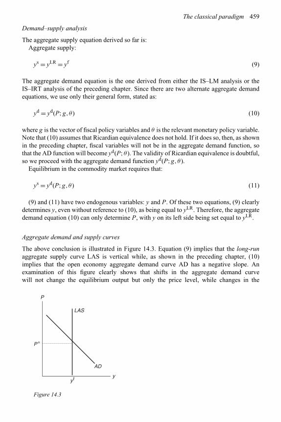
The classical paradigm 459
Demand–supply analysis
The aggregate supply equation derived so far is:Aggregate supply:
ys = yLR = yf (9)
The aggregate demand equation is the one derived from either the IS–LM analysis or theIS–IRT analysis of the preceding chapter. Since there are two alternate aggregate demandequations, we use only their general form, stated as:
yd = yd(P;g,θ ) (10)
where g is the vector of fiscal policy variables and θ is the relevant monetary policy variable.Note that (10) assumes that Ricardian equivalence does not hold. If it does so, then, as shownin the preceding chapter, fiscal variables will not be in the aggregate demand function, sothat the AD function will become yd(P;θ ). The validity of Ricardian equivalence is doubtful,so we proceed with the aggregate demand function yd(P;g,θ ).
Equilibrium in the commodity market requires that:
ys = yd(P;g,θ ) (11)
(9) and (11) have two endogenous variables: y and P. Of these two equations, (9) clearlydetermines y, even without reference to (10), as being equal to yLR. Therefore, the aggregatedemand equation (10) can only determine P, with y on its left side being set equal to yLR.
Aggregate demand and supply curves
The above conclusion is illustrated in Figure 14.3. Equation (9) implies that the long-runaggregate supply curve LAS is vertical while, as shown in the preceding chapter, (10)implies that the open economy aggregate demand curve AD has a negative slope. Anexamination of this figure clearly shows that shifts in the aggregate demand curvewill not change the equilibrium output but only the price level, while changes in the
P
y fy
AD
LAS
P∗
Figure 14.3
460 Monetary policy and the macroeconomy
aggregate supply will change both output and price level. This is a very strong con-clusion and is, as we shall see later in this and the next three chapters, at the heartof the debate on the ineffectiveness of monetary and fiscal policies for the equilibriumstates of the neoclassical model and its related modern classical and new classicalmodels.
Equilibrium output and prices
Equations (9) to (11) determine the long-run equilibrium values of output y and price levelP from:
yLR = yf (12)
P = f (g,θ;yLR) (13)
so that monetary and fiscal policies can change aggregate demand and the price level, but notlong-run output. In the presence of Ricardian equivalence, P = f (θ,yLR), so that changes inmonetary policy and in yLR can change the price level, but fiscal policy cannot do so.
In terms of the general equilibrium neoclassical model, (12) determines output and (13)determines the price level. These equations imply the aggregate demand, monetary and fiscalmultipliers on output as:
∂yLR/∂yd = 0, ∂PLR/∂yd > 0 (14)
∂yLR/∂g = 0, ∂PLR/∂g ≥ 0 (15)6
∂yLR/∂θ = 0, ∂PLR/∂θ > 0 (16)
which clearly indicate that the long-run equilibrium level of output is not responsive tomonetary policies, whereas that of the price level is responsive to these policies.7 This alsoapplies to fiscal policies, except under Ricardian equivalence when fiscal policy affects neitheraggregate demand nor output nor the price level.
Supply shifts
The impact of a change in output on the price level, represented by ∂P/∂yLR, is negative inboth the IS–LM and IS–IRT models, though its magnitude depends on whether the moneysupply or the interest rate is the exogenous monetary policy variable. The basic reason forthe negative impact of output increases on the price level is that an increase in output raisesthe transactions demand for money, which has to be offset by lower prices. We leave it to theinterested reader to derive ∂P/∂y for the IS–LM and IS–IRT models, using the informationgiven in this and the last chapter.
6 ∂PLR/∂g = 0 if Ricardian equivalence holds.7 This model can also be used to derive the quantity theory proposition that, in equilibrium, a change in
the money supply causes a proportionate change in the price level, even though the neoclassical modelencompasses the interest sensitivity of money demand – and therefore allows for a positive speculative demand formoney.
The classical paradigm 461
14.4 Iterative structure of the neoclassical model
Another procedure for studying simultaneous equilibrium in all sectors of the economyemerges if the final equilibrium equation for each of the sectors is examined separately inthe overall problem. The following equations (17) to (22) incorporate information on all thesectors.Production–employment sector:
y = yf (17)
The commodity market IS equation:
y=y(r,P;g,θ )=
⎛⎜⎜⎝ 1
1−cy +cyty + 1
ρrzcy(1−ty)
⎞⎟⎟⎠·
({c0−cyt0+i0−irr+g+xc0−xcρρr}+ 1
ρr
{−zc0+zcyt0−zcρρr})(18)
Fisher equation:
R = (1 + r)(1 +πe) (19)
From the employment–output sector equilibrium, we know that the long-run equilibriumoutput is yf. Substitute this equilibrium level of output into the IS relationship (18), whichyields the long-run equilibrium real rate of interest as rLR
0:
rLR0 = 1
ir
((c0 − cyt0 + i0 + g0 + xc0 − xcρρr)+ 1
ρr
(−zc0 + zcyt0 − zcρρr))
−
(1 − cy + cyty + 1
ρrzcy(1 − ty)
)ir
yf (20)
We now know the long-run equilibrium level of the real interest rate, even without introducingthe monetary sector into the analysis so far.
Money market equilibrium depends on whether the central bank uses the interest rate orthe money supply as the exogenous monetary policy variable. The relevant equations are:LM equation in the IS–LM model:
�M/P = myy + (FW0 − mRR) (21)
Money market equilibrium condition in the IS–IRT model:
M/P = myy + (FW0 − mRR) (22)
The following analysis deals separately with each of these cases.
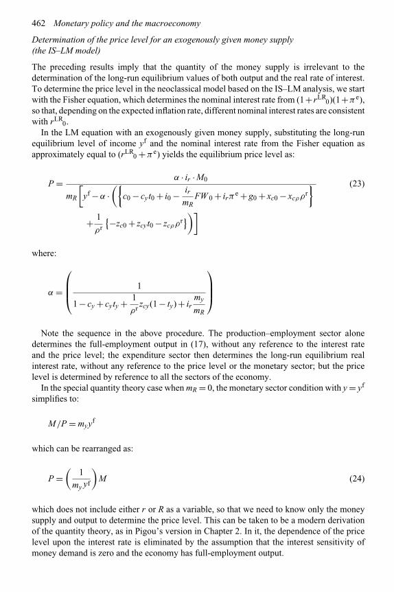
462 Monetary policy and the macroeconomy
Determination of the price level for an exogenously given money supply(the IS–LM model)
The preceding results imply that the quantity of the money supply is irrelevant to thedetermination of the long-run equilibrium values of both output and the real rate of interest.To determine the price level in the neoclassical model based on the IS–LM analysis, we startwith the Fisher equation, which determines the nominal interest rate from (1+ rLR
0)(1+πe),so that, depending on the expected inflation rate, different nominal interest rates are consistentwith rLR
0.In the LM equation with an exogenously given money supply, substituting the long-run
equilibrium level of income yf and the nominal interest rate from the Fisher equation asapproximately equal to (rLR
0 +πe) yields the equilibrium price level as:
P = α · ir · M0
mR
[yf −α ·
({c0 − cyt0 + i0 − ir
mRFW 0 + irπe + g0 + xc0 − xcρρr
}
+ 1
ρr
{−zc0 + zcyt0 − zcρρr})]
(23)
where:
α =
⎛⎜⎜⎝ 1
1 − cy + cyty + 1
ρrzcy(1 − ty) + ir
my
mR
⎞⎟⎟⎠
Note the sequence in the above procedure. The production–employment sector alonedetermines the full-employment output in (17), without any reference to the interest rateand the price level; the expenditure sector then determines the long-run equilibrium realinterest rate, without any reference to the price level or the monetary sector; but the pricelevel is determined by reference to all the sectors of the economy.
In the special quantity theory case when mR = 0, the monetary sector condition with y = yf
simplifies to:
M/P = myyf
which can be rearranged as:
P =(
1
my yf
)M (24)
which does not include either r or R as a variable, so that we need to know only the moneysupply and output to determine the price level. This can be taken to be a modern derivationof the quantity theory, as in Pigou’s version in Chapter 2. In it, the dependence of the pricelevel upon the interest rate is eliminated by the assumption that the interest sensitivity ofmoney demand is zero and the economy has full-employment output.

The classical paradigm 463
Determination of the price level for an exogenously given interest rate(the IS–IRT model)
In the IS–IRT model of the preceding chapter, it was assumed that the central bank sets thereal interest rate, with its level specified as rT
0. Aggregate demand yd is then given by thecommodity market at the given real interest rate. This AD equation is:
yd = y(r T0 ,P;g,θ ) =
⎛⎜⎜⎝ 1
1 − cy + cyty + 1
ρrzcy(1 − ty)
⎞⎟⎟⎠ ·
({c0 − cyt0 + i0 − irr
T0 + g + xc0 − xcρρr
}
+ 1
ρr
{−zc0 + zcyt0 − zcρρr}) (25)
Given output supply at yf, and the real interest rate at rT, this equation determines the pricelevel P.
Policy implications: the ineffectiveness of monetary and fiscal policies in changingoutput and employment
Important policy implications follow from the iterative nature in the long-run equilibriumof the neoclassical model. No matter what is the monetary policy variable, neither monetarynor fiscal policies can affect equilibrium output, since neither appears in (17). Therefore,these policies are useless for increasing the long-run equilibrium levels of employment andreducing the equilibrium level of unemployment. However, with the economy in long-runequilibrium, these policies are not only useless, they are also not needed since the long-runequilibrium employment is at full employment. Hence, in the long run, there is no need orscope for the authorities to pursue policies to increase employment or output, which are bothat their full-employment levels. Any such attempt will be ineffective.
If we compare these implications on the irrelevance of monetary and fiscal policies foroutput and employment with the stylized facts, these implications are clearly invalid. Expan-sionary monetary and fiscal policies do increase aggregate output and lower unemployment,and the reverse is true for contractionary policies. Therefore, the preceding model needs tobe modified in order to be valid and useful. The classical economists do this, as explainedlater, by introducing uncertainty, with errors or misperceptions in expectations, into themodel.
14.4.1 The rate of unemployment and the natural rate of unemployment
The level of unemployment is defined as:
U = L − n (26)
where:U = level of unemploymentL = labor force.
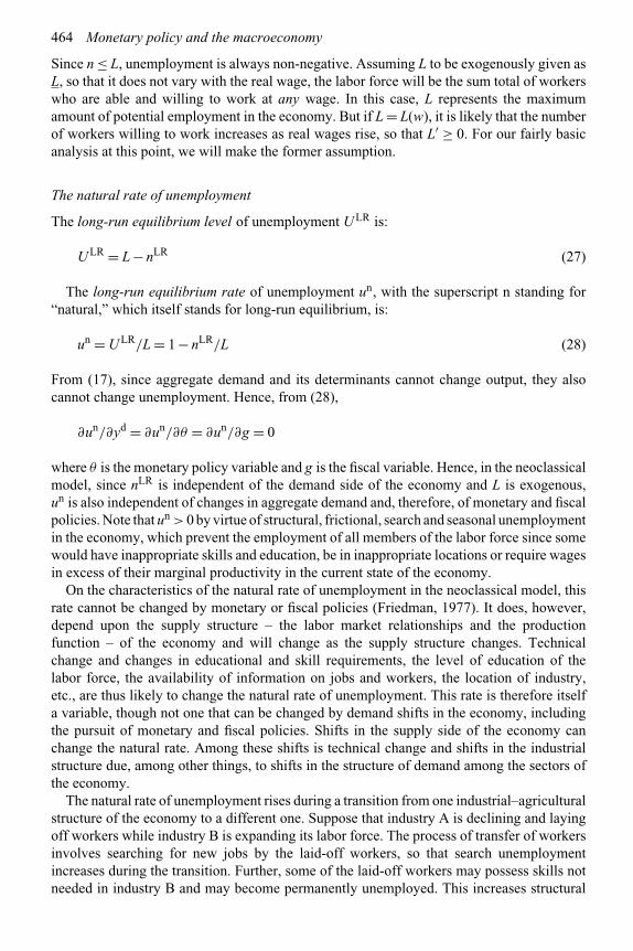
464 Monetary policy and the macroeconomy
Since n ≤ L, unemployment is always non-negative. Assuming L to be exogenously given asL, so that it does not vary with the real wage, the labor force will be the sum total of workerswho are able and willing to work at any wage. In this case, L represents the maximumamount of potential employment in the economy. But if L = L(w), it is likely that the numberof workers willing to work increases as real wages rise, so that L′ ≥ 0. For our fairly basicanalysis at this point, we will make the former assumption.
The natural rate of unemployment
The long-run equilibrium level of unemployment ULR is:
ULR = L − nLR (27)
The long-run equilibrium rate of unemployment un, with the superscript n standing for“natural,” which itself stands for long-run equilibrium, is:
un = ULR/L = 1 − nLR/L (28)
From (17), since aggregate demand and its determinants cannot change output, they alsocannot change unemployment. Hence, from (28),
∂un/∂yd = ∂un/∂θ = ∂un/∂g = 0
where θ is the monetary policy variable and g is the fiscal variable. Hence, in the neoclassicalmodel, since nLR is independent of the demand side of the economy and L is exogenous,un is also independent of changes in aggregate demand and, therefore, of monetary and fiscalpolicies. Note that un > 0 by virtue of structural, frictional, search and seasonal unemploymentin the economy, which prevent the employment of all members of the labor force since somewould have inappropriate skills and education, be in inappropriate locations or require wagesin excess of their marginal productivity in the current state of the economy.
On the characteristics of the natural rate of unemployment in the neoclassical model, thisrate cannot be changed by monetary or fiscal policies (Friedman, 1977). It does, however,depend upon the supply structure – the labor market relationships and the productionfunction – of the economy and will change as the supply structure changes. Technicalchange and changes in educational and skill requirements, the level of education of thelabor force, the availability of information on jobs and workers, the location of industry,etc., are thus likely to change the natural rate of unemployment. This rate is therefore itselfa variable, though not one that can be changed by demand shifts in the economy, includingthe pursuit of monetary and fiscal policies. Shifts in the supply side of the economy canchange the natural rate. Among these shifts is technical change and shifts in the industrialstructure due, among other things, to shifts in the structure of demand among the sectors ofthe economy.
The natural rate of unemployment rises during a transition from one industrial–agriculturalstructure of the economy to a different one. Suppose that industry A is declining and layingoff workers while industry B is expanding its labor force. The process of transfer of workersinvolves searching for new jobs by the laid-off workers, so that search unemploymentincreases during the transition. Further, some of the laid-off workers may possess skills notneeded in industry B and may become permanently unemployed. This increases structural

The classical paradigm 465
unemployment in the economy. That is, the shift in the economy’s industrial structure inducesa transitional increase in the natural rate of unemployment, but it can also imply a long-runshift in that rate.
14.4.2 IS–LM version of the neoclassical model in a diagrammatic form
Figure 14.3 brings together the information in equations (17) to (22). (18) to (22) specify thedownward-sloping AD curve. From (17), since output does not depend on P, the aggregatesupply (AS) curve is vertical at yf. It is often called the “full-employment (yf) curve.”Equilibrium in all the sectors of the economy exists at the point (P∗, yf).
An expansionary monetary policy with an exogenous money supply(the IS–LM model)
Figure 14.4 illustrates the IS–LM model in the (r, y) space. Equation (17) specifies the LAScurve at the full-employment output yf, (18) specifies the IS curve, and (19) and (21) are usedto specify the LM curve. The intersection of the IS and LM curves determines the level ofaggregate demand. General equilibrium in the commodity, money and output sectors requiresthat all three curves intersect at the same point. This is the case shown in Figure 14.4.
We next provide some examples of how the IS–LM analysis and diagram can bemanipulated for comparative static studies. This is done in Figure 14.5 for monetary policy.Suppose that the economy is initially in overall equilibrium at the point a and the moneysupply increases, shifting the LM curve from LM0 to LM1. The new equilibrium betweenthe monetary and expenditure sectors is shown by the point d and represents nominalaggregate demand. But output specified by the output–employment sector is at yf. Sinceaggregate demand at d exceeds the supply of output yf, prices rise. As P rises, the LM curveshifts towards the left. However, the rise in P leaves the IS and AS curves unchanged.Prices will then continue to rise as long as aggregate demand for output exceeds itssupply. This will occur until the leftward shifts in the LM curve due to the price increasestake it sufficiently back (i.e. from LM1 to LM1
′) to pass through the initial equilibriumpoint a. In short, in terms of equilibrium states, an increase in the money supply increases
y f
a
r
y
IS
LMLAS
Figure 14.4

466 Monetary policy and the macroeconomy
y -n
a
y f yd1
r
y
IS
LM1
d
LM0,LM1′
Figure 14.5
d
b
r
y
IS1
LMy-n
IS0
y f yd1
LM ′
Figure 14.6
aggregate demand, without affecting output, and raises prices to a new level, with theincrease in the price level being proportionate to the increase in the money supply. Theinterest rate is unchanged between the old and the new equilibrium positions. Comparingthese implications with the stylized facts given at the beginning of this chapter shows thatthey are not valid for the short run. Therefore, the model presented so far needs to bemodified.
An expansionary fiscal policy with an exogenous money supply
Now suppose that fiscal policy had become expansionary with an increase in governmentexpenditures. This would have increased the real aggregate demand for commodities andshifted the IS curve from IS0 to IS1 in Figure 14.6. Nominal aggregate demand at the point d(at the intersection of the IS1 and LM curves) exceeds output yf. Prices rise, eventually liftingthe LM curve to a new overall equilibrium at point b, with the final LM curve as LM ′. Bothprices and interest rates are higher in the new equilibrium position at b than at the initial oneat point a. Hence, increases in fiscal expenditures increase the equilibrium levels of interestrates and prices. However, they do not change output. The last implication is clearly not validfor the short run.

The classical paradigm 467
14.5 Fundamental assumptions of the Walrasian equilibrium analysis
The preceding analysis has focused on the long-run equilibrium states of the model and is asuccinct macroeconomic version of the Walrasian model in the absence of uncertainty. Thisequilibrium analysis makes four fundamental assumptions, plus a fifth one that specifies thatthe findings are for the certainty case. These are:
(I) Flexible prices and wages, and the stability of marketsThe prices of all the goods in the economy are assumed to be flexible and adjust toequate demand and supply in the relevant market. They increase if there is excessdemand and decrease if there is excess supply. These prices include wages, which isthe price of labor. Wages are flexible in both nominal and real terms.
(II) Perfect market hypothesis8
Each market has perfect competition and clears continuously, so that we can focus onthe study of competitive general equilibrium in the economy and its properties, whilelargely ignoring the disequilibrium values of the variables.
(III) Transparency of equilibrium pricesAll agents, in making their demand and supply decisions, assume that such marketclearance will occur instantly after any disturbance and know or anticipate (or areinformed by an agency such as a “Walrasian auctioneer” or “market coordinator”) theprices at which it will occur. Further, all agents plan to produce, consume, demandmoney and supply labor at only these equilibrium prices.9
(IV) Notional demand and supply functionsAll economic agents assume that they will be able to buy or sell as much as they want toat the long-run equilibrium prices. The demand and supply functions derived under thisassumption are known as notional (as against effective) demand and supply functions.
The Walrasian-based models now also include:(V) Assumptions on uncertainty
If the model assumes certainty, its results provide the long-run equilibrium of theeconomy. Its extension to include uncertainty will produce deviations from this long-run equilibrium, with the nature of the deviations depending on the way uncertainty ishandled in the extended model. When the equilibrium of the economy under uncertaintydiffers from the long-run equilibrium of the model, such an equilibrium is designatedas a short-run equilibrium. One of the causes of such a deviation from the long-runequilibrium is errors in price expectations. However, there can also be many othercauses of such deviations.
The current versions of the Walrasian-based macroeconomic models assume therational expectations hypothesis, with the long-run general equilibrium outcomes usedto specify the rationally expected values of the relevant variables.
The classical equilibrium analysis of the economy and its policy recommendations requirethe applicability of the above fundamental assumptions: flexible prices and wages, continuous
8 A market is perfect if it has perfect competition and is fully efficient, which is defined as continuous/instantaneousmarket clearance. Therefore, a market can be competitive but have slow adjustment of prices, so that it is notefficient.
9 In particular, if there are delays in establishing these prices or communicating their knowledge, it is assumedthat all production and trade are put on hold during the delay and that any such delay does not impose costs oneconomic agents. This is known as recontracting.

468 Monetary policy and the macroeconomy
market clearance, transparency of equilibrium prices and notional demand and supplyfunctions. Each assumption is related to the others but is still distinct. Any one or moreof these assumptions may not be relevant to or valid for a particular stage or at a particulartime in an economy.
As shown above, monetary policy is neutral in the long-run equilibrium states of theneoclassical model since changes in monetary policy affect only the nominal but not thereal variables. Hence, the neoclassical model implies that, in its long-run equilibrium,monetary policy cannot change output and employment in the economy. In fact, with theeconomy at full employment, there is also no need for the pursuit of monetary policy.Conversely, if the above assumptions hold, changes in the money supply also cannot bedetrimental for long-run output and employment in the economy. In particular, decreasesin the money supply will not decrease output and employment and force the economyinto a recession. Monetary policy is benign (harmless) in such a context. Note that theseare assertions about the long-run analytical state, not about the short-run equilibrium ordisequilibrium.
14.6 Disequilibrium in the neoclassical model and the non-neutralityof money
Note that the neoclassical model does not assert that its long-run equilibrium must alwaysexist – as if it were an identity – and therefore it allows the possibility that the economycan be sometimes in short-run equilibrium or in disequilibrium. Further, for the studyof disequilibrium to be a potentially useful exercise requires the belief that the economywill be away from its full-employment equilibrium state for significant periods of time.Intuitively, continuous general equilibrium requires, for example, the belief that an increasein the money supply immediately causes a proportionate increase in the price level and thata decrease in the money supply does not cause a recession in output and employment. Thereis considerable evidence to show that these requirements are not always, or most of the time,met in most real-world economies. Nor did the major proponents in the traditional classicaland neoclassical tradition claim that they did. Among those who allowed for the existence ofdisequilibrium for significant periods of time, and the impact of money supply changes onoutput (i.e. the non-neutrality of money) during disequilibrium, were Hume, Marshall, Fisherand Pigou in the traditional classical school, and Friedman and the St Louis monetarists inthe neoclassical one.
However, when the classical economists allowed for disequilibrium, they maintainedthat any such state of disequilibrium incorporates certain forces brought about by markets(not firms) that will force the economy into equilibrium. Among these forces are pricechanges and the Pigou effect, including the real balance effect. These were touched upon inChapter 3 and will be explored more fully in Chapter 18. We explain them again, thoughbriefly, in the following subsection as a reminder and for completeness of the neoclassicalmodel.
14.6.1 Pigou and real balance effects
The Pigou effect is associated with the contributions of A.C. Pigou (at Cambridge Universityin England in the first half of the twentieth century) in the debate between the traditionalclassical school and Keynes in the 1930s. The Pigou effect is another name for the effect of
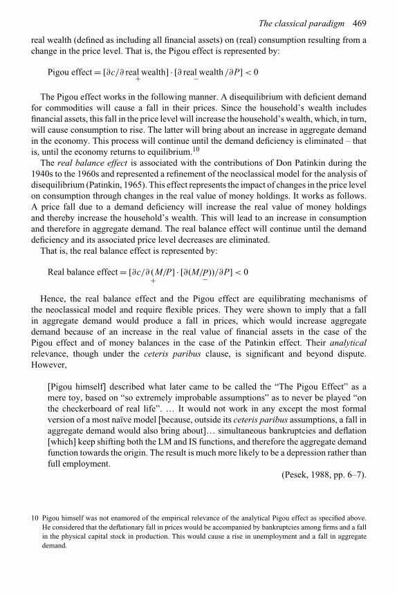
The classical paradigm 469
real wealth (defined as including all financial assets) on (real) consumption resulting from achange in the price level. That is, the Pigou effect is represented by:
Pigou effect = [∂c/∂ real wealth+ ] · [∂ real wealth− /∂P] < 0
The Pigou effect works in the following manner. A disequilibrium with deficient demandfor commodities will cause a fall in their prices. Since the household’s wealth includesfinancial assets, this fall in the price level will increase the household’s wealth, which, in turn,will cause consumption to rise. The latter will bring about an increase in aggregate demandin the economy. This process will continue until the demand deficiency is eliminated – thatis, until the economy returns to equilibrium.10
The real balance effect is associated with the contributions of Don Patinkin during the1940s to the 1960s and represented a refinement of the neoclassical model for the analysis ofdisequilibrium (Patinkin, 1965). This effect represents the impact of changes in the price levelon consumption through changes in the real value of money holdings. It works as follows.A price fall due to a demand deficiency will increase the real value of money holdingsand thereby increase the household’s wealth. This will lead to an increase in consumptionand therefore in aggregate demand. The real balance effect will continue until the demanddeficiency and its associated price level decreases are eliminated.
That is, the real balance effect is represented by:
Real balance effect = [∂c/∂ (+M/P] · [∂(M/P−))/∂P] < 0
Hence, the real balance effect and the Pigou effect are equilibrating mechanisms ofthe neoclassical model and require flexible prices. They were shown to imply that a fallin aggregate demand would produce a fall in prices, which would increase aggregatedemand because of an increase in the real value of financial assets in the case of thePigou effect and of money balances in the case of the Patinkin effect. Their analyticalrelevance, though under the ceteris paribus clause, is significant and beyond dispute.However,
[Pigou himself] described what later came to be called the “The Pigou Effect” as amere toy, based on “so extremely improbable assumptions” as to never be played “onthe checkerboard of real life”. … It would not work in any except the most formalversion of a most naïve model [because, outside its ceteris paribus assumptions, a fall inaggregate demand would also bring about]… simultaneous bankruptcies and deflation[which] keep shifting both the LM and IS functions, and therefore the aggregate demandfunction towards the origin. The result is much more likely to be a depression rather thanfull employment.
(Pesek, 1988, pp. 6–7).
10 Pigou himself was not enamored of the empirical relevance of the analytical Pigou effect as specified above.He considered that the deflationary fall in prices would be accompanied by bankruptcies among firms and a fallin the physical capital stock in production. This would cause a rise in unemployment and a fall in aggregatedemand.

470 Monetary policy and the macroeconomy
Further, the analyses of the real balance and the Pigou effects do not, a priori, provide anyguidance on the time the neoclassical economy will need to return to long-run equilibriumunder their impetus. In particular, the real balance effect can be quite weak, so that theneoclassical economy could react to an exogenous fall in demand by a very slow movementtowards long-run equilibrium and, therefore, remain away from it for a significant period.Hence, it is important to analyze the short run and disequilibrium properties of the neoclassicalmodel and derive its policy implications.
Macroeconomic theory uses two main channels for the effects of money supply changes onaggregate demand. One of these is because changes in the money supply change wealth andreal balances, which changes consumption expenditures (the direct transmission channel).The other is through the effect of money supply changes on interest rates, which changesinvestment expenditures (the indirect transmission channel). The direct effects are consideredto be relatively small over the business cycle, so that most macroeconomic models, includingthe popular IS–LM one, ignore them altogether.11 Consequently, these models embody onlythe indirect transmission channel of monetary policy effects through interest rates.
14.6.2 Causes of deviations from long-run equilibrium
The actual economy may not be in or close to its long-run equilibrium because of:
1 Errors in expectations, either in the commodity or/and in labor markets. The analysisof this scenario is presented in the next section on the short-run equilibrium of theneoclassical model.
2 Costs of adjusting prices, wages, employment and output. The analyses of these variousscenarios are presented in the next chapter on the Keynesian paradigm.
3 The absence of a mechanism for instantly restoring equilibrium. Note that the assumptionof perfect competition does not a priori specify the chronological time needed bythe “invisible hand of competition” to return an economy, following a shock, to itsfull-employment equilibrium.12 Along with the absence of a mechanism for instantlyrestoring the full-employment equilibrium, the competitive economy also does not havean instantaneous mechanism operating in disequilibrium for computing the new pricelevel and informing all firms and households of the new prices of the products. Further,there is no guarantee given to the firms that they could sell all they wanted at these prices,nor is there any guarantee that the workers will receive or recoup the incomes lost whilethey were unemployed. Combining this lack of a guarantee with the plausible possibilitythat firms and households may respond faster than markets to disequilibrium and willdo so on the basis of expectations of the quantity demanded and jobs available, couldproduce a disequilibrium path that keeps the economy out of equilibrium for quite some(chronological) time. This scenario is sketched in the next chapter.
4 Firms are in monopolistic competition with sticky prices (see Chapter 15).
11 This implies that consumption is independent of money balances, which requires that the utility function overgoods be separable between commodities and money balances. Empirically, Ireland (2001a) finds little supportfor a non-separable utility function for US data.
12 Because of this, the Walrasian and neoclassical models were buttressed with some deus ex machina such as theWalrasian auctioneer, tâtonnement (i.e. the process of “groping” towards equilibrium) and recontracting, whichsolved the problem analytically but represented an escape from answering the relevant question of how long ittakes the real-world economies to return to equilibrium.

The classical paradigm 471
14.7 The relationship between the money supply and the price level:the heritage of ideas
The basic comparative static conclusions of the neoclassical macroeconomic model of thischapter were presented several centuries ago. The following quote illustrates them from thewritings of David Hume, one of the founders of classical economics.
Money is nothing but the representation of labor and commodities, and serves only asa method of rating or estimating them. Where coin is in greater plenty – as a greaterquantity of it is required to represent the same quantity of goods – it can have no effect,either good or bad, taking a nation within itself; any more than it would make an alterationin a merchant’s books, if instead of the Arabian method of notation, which requires fewcharacters, he should make use of the Roman, which requires a great many.
(Hume, Of Money, 1752).
This quote is an assertion of the basic proposition of the quantity theory of money: anincrease in the money supply causes a proportional increase in prices. Further, Hume assertsthat changes in the supply of money do not change real output in the economy but correspondto a change in the unit of account. The quantity theory was presented in Chapter 2.
The conclusions of this theory on the proportionate relationship between the money stockand prices, and the inability of the monetary and fiscal authorities to control output andemployment, apply in equilibrium. They do not necessarily apply in disequilibrium – thatis, during the adjustment from one equilibrium to another. In fact, many supporters of thistheory, in Hume’s time and down to the present, have viewed changes in the money stock asexerting a powerful influence on output, employment and other variables in the adjustmentprocess. Hume himself described this process as follows.
Notwithstanding this conclusion, which must be allowed just, it is certain that since thediscovery of the mines in America, industry has increased in all the nations of Europe,except in the possessors of those mines; and this may justly be ascribed, among otherreasons, to the increase of gold and silver. Accordingly, we find that in every kingdom,into which money begins to flow in greater abundance than formerly, everything takeson a new face; labor and industry gain life; the merchant becomes more enterprising,and even the farmer follows his plough with greater alacrity and attention…
To account then for this phenomenon, we must consider, that though the high priceof commodities be a necessary consequence of the increase of gold and silver, yet itfollows not immediately upon that increase; but some time is required before the moneycirculates through the whole state, and makes its effect be felt on all ranks of people.At first, no alteration is perceived; by degrees the price rises, first of one commodity,then of another; till the whole at last reaches a just proportion with the new quantity ofspecie which is in the kingdom. In my opinion, it is only in this interval or intermediatesituation, between the acquisition of money and the rise of prices, that the increasingquantity of gold and silver is favorable to industry.
(Hume, Of Money, 1752).
Hume’s opinions on the disequilibrium path of adjustment serve as a note of cautionagainst total reliance on the comparative static results of the neoclassical model and againstthe belief that the pre-1936 classical economists assumed that the economy always functions

472 Monetary policy and the macroeconomy
in full employment. Hume’s analysis of disequilibrium shows that the economy can be indisequilibrium for some time and that money will not be neutral during this period.
Almost two centuries later, Pigou, a twentieth-century economist in the classical tradition,expressed similar ideas in the following excerpts from his book, Money, A Veil (1941).
Money – the institution of money – is an extremely valuable social instrument, makinga large contribution to economic welfare. … if there were no generally accepted money,many of these transactions would not be worth undertaking, and as a direct consequencethe division of labor would be hampered and less services and goods would be produced.Thus, not only would real income be allocated less satisfactorily, from the standpointof economic welfare, among different sorts of goods, but it would also contain smalleramounts of many, if not of all sorts. … Obviously then money is not merely a veil or agarment or a wrapper. Like the laws of property and contract, it constitutes at the leasta very useful lubricant, enabling the economic machine to function continuously andsmoothly. …
So far everyone would be agreed. But now an important distinction must be drawn.The institution of money is, as we have seen, a powerful instrument promoting wealthand welfare. But the number of units of money embodied in that instrument is, in general,of no significance. It is all one whether the garment, or the veil, is thick or thin. I donot mean, of course, that it is immaterial whether the number of units of money is heldconstant, or is variable in one manner, or is variable in another manner in relation toother economic happenings. I mean that if, other things being equal, over a series ofmonths or years the stock of money contains successively m×1, m×2, m×3. … units,it makes no difference what the value of m is. A doubled value of m throughout meanssimply doubled prices throughout of every type of goods – subject, of course, to the rateof interest not being reckoned for this purpose as a price – and all real happenings areexactly what they would have been with a value of m half as large. The reason for thisis that, money being only useful because it exchanges for other things, a larger quantitydoes not, as with other things, carry more satisfaction on its back than a smaller quantity,but the same satisfaction.
(Pigou, 1941, Ch. 4).
In this quote, Pigou is clearly expressing the long-run equilibrium results following anincrease in the money supply. Note that what is missing in this story are Hume’s conclusionson the impact of changes in the money supply during the ensuing adjustment period. However,as his other writings show, Pigou was quite aware of such an adjustment period and of theimpact of money supply variations in causing fluctuations in employment and output.
14.8 The classical and neoclassical tradition, economic liberalismand laissez faire
The long-run equilibrium analysis of the neoclassical model in this chapter implies that theeconomy functions at full employment, with full-employment output, so that there is no scopefor monetary and fiscal demand management policies for such an economy. Such a viewpointis part of the classical philosophy of economic liberalism, which can be broadly formulatedas stating that the economy performs at its best by itself and that the state cannot improve onits performance. This is usually also supplemented by the proposition that any interventionby the state, even with the intention of improving upon the performance of the economy,
The classical paradigm 473
worsens its performance. These propositions imply that the goods and input markets shouldbe free and that free enterprise should be the desired standard. However, market imperfectionssuch as imperfect competition, oligopoly, monopoly or monopsony, externalities, etc., couldand often do exist in the actual economy. Advocates of the strong form of economic liberalismargue that, even in such cases, the economy should be left as it is and the state should notattempt to eliminate such imperfections; the imperfections are minor and, even when theyare not of minor significance, there is no guarantee that state intervention will achieve a netimprovement since its intervention might eliminate some imperfections while introducingothers. A weaker version of economic liberalism allows the state to intervene to eliminatemarket imperfections through selective policies, though without assigning a role to generalmonetary and fiscal policies.
To be credible, the general liberalism philosophy has its underpinnings in the nation’spolitical, economic and social ideology, and in the public’s perception and goals for theactual economic and social performance of the nation. In its general approach, the underlyingphilosophical basis of liberalism was provided by the utilitarianism approach of JeremyBentham and his followers in the first half of the nineteenth century. The main tenet ofthis approach was that economic agents (households and firms), working in their own bestinterests (utility and profit maximization), would ensure that social welfare was maximized.13
Consequently, the economy should be left alone by the government and regulatory agencies.This policy approach was summarized in the term laissez faire. In its economic aspects, theliberalism philosophy needed a theoretical economic model that could justify its economicpolicy recommendations. This model was provided at the macroeconomic level by thetraditional classical approach in the pre-Keynesian period and is currently the neoclassicalone – with the modern and new classical models among its versions.
The economic and social problems of nineteenth-century Britain, with rapid industrializa-tion and urbanization, were sufficiently acute and transparent to lead to a gradual evolutionof political and economic thought away from liberalism and laissez faire and towards someform of socialism, with support for some degree of state intervention in the economy.This evolution of ideas was widespread during the latter half of the nineteenth centuryand early twentieth century. The Great Depression of the 1930s destroyed the public’s andeconomists’ faith in laissez faire, so that Keynes’s publication of The General Theory in1936, with its encouragement to the state to use monetary and fiscal policies to improveon a poorly performing economy, proved to be timely and readily won acceptance frommost economists and the public. Economic liberalism was eclipsed by Keynesianism for thedecades from the 1930s to the 1970s. The Keynesian approach is the subject of the nextchapter.
In economics, the traditional classical ideas were reformulated and rebottled in the formof the neoclassical theory during the decades of the 1940s to the 1970s. Since the 1970s,these ideas, in the form of the modern classical model and with the agenda of makingmicroeconomics the foundation of macroeconomics, have again become the dominantapproach in macroeconomics. Their return to this dominance detoured briefly throughMonetarism during the 1970s. They are currently supported by the new classical approachdeveloped during the 1970s and the 1980s.
13 The high rates of poverty, even among the “working poor,” and of unemployment in Britain during the heydayof laissez faire economics led the nineteenth-century social reformer, Thomas Carlyle, to label economics asthe “dismal science.” This name for economics still remains as one of its nicknames.

474 Monetary policy and the macroeconomy
14.8.1 Some major misconceptions about traditional classical and neoclassicalapproaches
A common misconception nowadays is that the traditional classical and neoclassicaleconomists believed that the economy functioned well enough to maintain full employmentmost of the time or that it had a fast tendency to return to full employment following adisturbance and a decline in employment. In fact, many believed that “the economic systemis essentially unstable” (Patinkin, 1969, p. 50).14 Another misconception nowadays is thatthe classical and neoclassical economists believed that money was neutral in practice and intheory. In fact, as the business cycle literature of the nineteenth and early twentieth centuriesamply shows, it was a common and strongly held belief that fluctuations in the money supplywere a major cause of recessions, with declines in employment and output, and of booms inreal economic activity.
During the period of traditional classical dominance (mid-eighteenth century to 1936),booms and recessions were common and sometimes quite severe. It was a commonobservation among economists that the velocity of circulation of money did change, and didso over booms and recessions. In fact, many economists believed that there could occur – anddid occur – “extreme alternations of hoarding and dishoarding” (p. 50) because of changesin expectations, and that the changes in the money supply and in its velocity were majorsources of business fluctuations, as attested by Don Patinkin (1972). Further, many economistsbelieved that these fluctuations were:
exacerbated by the “perverse” behavior of the banking system, which expands credit inbooms and contracts it in depressions.
(Patinkin, 1969, p. 51).
Among the reasons for the real effects of money supply and velocity changes was that:
Costs have a tendency to move more slowly than do the more flexible selling prices[i.e. firms’ costs were sticky relative to their final prices]
(Patinkin, 1969, p. 57).
Sticky prices are peculiarly resistant to downward pressure. … [To sum up, itwas generally recognized that] cycles and depressions [are] an inherent feature of“capitalism.” Such a system must use money, and the circulation of money is not aphenomenon which naturally tends to establish and maintain an equilibrium level. Itsequilibrium is vague and highly unstable.
(Patinkin, 1969, pp. 63–64).
In view of such strong effects of money supply variations on employment and output, whatthe traditional classical economists believed was that money was neutral in the long run, butnot in the short run or over the business cycle. Its neutrality in the long run was often less a
14 The various quotes are taken from Patinkin (1969), even though many of them are from passages quoted by himfrom other writers such as Henry Simons, Frank Knight and other economists at the University of Chicago inthe second quarter of the twentieth century and presumably part of the Chicago tradition of classical economics.Patinkin (1972) provides another source of the points made in these paragraphs. Parkin (1986) provides anevaluation of Patinkin’s views.

The classical paradigm 475
matter of analysis than of belief, which was sometimes reflected in the proposition known asSay’s law (see Chapter 18).
On policy issues, in view of the reasons given above, the traditional classical schoolbelieved that:
The government has an obligation to undertake a contracyclical policy. The guidingprinciple of this policy is to change M so as to offset changes in V, and thus generatethe full employment level of aggregate demand MV.
Once a deflation has gotten under way, in large modern economy, there is no significantlimit which the decline of prices cannot exceed, if the central government fails to use itsfiscal powers generously and deliberately.
(Patinkin, 1969, pp. 51, 63).
As the preceding quotes from Patinkin, a foremost neoclassical economist, convincinglyshow, monetary policy was often envisaged and recommended as a stabilization tool. Fiscalpolicy was sometimes, but not commonly, considered a possibility since pre-1936 economicanalysis did not have its analytical basis nor did it have a theory of the aggregate demand forcommodities. The analytical basis for fiscal policy and its recommendation as a major toolfor stabilization of aggregate demand were due to Keynes and the Keynesians. As a counter-reformation, Barro’s Ricardian equivalence theorem (Barro, 1974; see also Chapter 13,Section 13.7) sought to again remove fiscal policy from the set of potential stabilizationtools.
14.9 Uncertainty and expectations in the classical paradigm
The analysis of the neoclassical model so far shows that many of its implications arecontradicted by the stylized facts. In particular, monetary and fiscal policies do change outputand unemployment, as against the model’s implication that they do not. Therefore, the modelhas to be modified. Classical economists do so by introducing uncertainty into the modeland relying on errors in prices expectations. The two models in this stream are the Friedmanmodel, which relies upon wage contracts and errors in price expectations in labor markets,and the Lucas model, which relies on expectational errors by firms in commodity markets.The following analyses deal with the nature of uncertainty and such errors.
The nature of risk, uncertainty and expectations in economics
Events whose outcomes are not known at the moment of decision making used to be classifiedin economics in the first half of the twentieth century into risky ones or uncertain ones. Thedifference between these terms was that an event involves risk if the objective probabilitiesof its outcomes exist and are known, whereas an event involves uncertainty if the objectiveprobabilities of its outcomes do not exist or are not known. Because of the nature of economicevents and/or because of the pervasive imperfection of knowledge involving future outcomes,few economic decisions involve known objective probabilities, so that the standard case ineconomics is one of uncertainty. However, probability theory finds it unmanageable to includemany of the elements of uncertainty such as the vagueness, inadequacy and imperfection ofinformation that distinguish uncertainty from risk. As a consequence, neoclassical economicsoften abandons the above distinction between risk and uncertainty, and treats the latter as ifit were really a case of risk, while Keynesian, especially post-Keynesian, economics often
476 Monetary policy and the macroeconomy
makes a strong distinction between them. For consistency with the literature relevant to thischapter, we shall use the word uncertainty as if it were synonymous with risk.
Note that for uncertain events, it can be validly postulated that the individual formssubjective probabilities of the anticipated outcomes, with such probabilities being basedon whatever knowledge the individual possesses or considers profitable to acquire. Suchknowledge can be highly inadequate and imperfect and even the range of anticipatedoutcomes can differ from the possible ones, so that the subjective probabilities held can behighly erroneous or volatile15 and would also differ among individuals. In general, classicalmacroeconomics ignores these problems with subjective probabilities.
Expectations hypotheses in macroeconomics
The two major hypotheses in economics for constructing the expected value of a variableare the adaptive expectations hypothesis and the rational expectations hypothesis (REH).The former is a statistical procedure, while the latter represents an economic theory ofexpectations. These approaches were used in Chapter 8 to estimate expected and permanentincome for the demand for money function. The hypothesis used in this chapter is that ofrational expectations, estimating the expected rate of inflation, the expected money supply orthe expected level of aggregate demand. The material in Chapter 8 on the rational expectationshypothesis should be reviewed at this stage.
Since the classical macroeconomic models assume that the economy will either stay inequilibrium or soon revert to it, the rationally expected levels of output, unemployment andprices, as of all other endogenous variables, are their long-run equilibrium (full-employment)levels. Their values can therefore be derived from the long-run solution of the model. Whilethis might be acceptable for analytical models that have their focus on the equilibrium valuesof the variables, the practice of monetary policy requires forecasts of the actual values ofthese variables at the time the policy will impact on them. Given the long lags in monetarypolicy, the relevant expectations even by the policy makers are often erroneous. From theperspective of nominal wage contracts, the economic agents must be able to forecast the pricelevel during the duration of the contract. Such forecasts often have errors, so that the real wagereceived usually differs from the real wage expected by firms and workers to accrue from thecontract. We next investigate the impact of expectations on wages, employment and output.
14.10 Expectations and the labor market: the expectations-augmentedPhillips curve
14.10.1 Output and employment in the context of nominal wage contracts
In industrialized economies, the nominal wage between a firm and its workers is established –whether explicitly negotiated or arrived at by implicit arrangement – ahead of the productionand employment decisions by the firm and before the actual price level is known. In arriving
15 Keynes (1936) emphasized the volatility of expectations in financial markets and, therefore, of the volatility ofthe speculative demand for money which is based on these expectations. This volatility, in turn, affected theimpact of monetary policy on the economy. The treatment of subjective probabilities as if they were objectiveones tends to ignore the vagueness and volatility of the former and misses their distinctive aspects and theirimpact on the economy. Keynes and post-Keynesians believe this impact to be important; neoclassical andmodern classical economists ignore it.
The classical paradigm 477
at the contracted nominal wage, firms and workers must base their agreement on the expectedreal wage – that is, the nominal wage divided by the expected price level – rather than the apriori unknown actual real wage which will apply at the time of employment and production.However, firms can continue to adjust their employment as the price level changes, so thattheir decisions on employment, as determined by their demand function for labor, will dependon the actual real wage – equal to the established nominal wage divided by the actual pricelevel. This section modifies the preceding neoclassical labor market analyses to incorporatethese ideas.
To start, consider the household utility maximization, as in Chapter 3, but now with theaddition of uncertainty about the future price level and with labor forming expectations on it.Let the household’s expected price level for the period ahead be Peh. Utility maximizationwould then imply that the supply function of labor is:
ns = ns(weh)
= ns(W/Peh) ns′ > 0 (29)
where:ns = labor supply functionweh = expected real wage, as expected by laborW = actual nominal wagePeh = price level expected by households or workers for the duration of the labor
contract
Designate the inverse of ns(.) as h(n), so that inverting (29) and rearranging yields:
W d = Peh · h(ns) h′ > 0 (30)
where W d is the wage demanded by workers in negotiations. Designate the representativefirm producing the i th product – and being in the i th market – as the i th firm. Prior to theproduction period, the profit-maximizing i th firm in perfect competition would equate itsmarginal product of labor to the expected real wage measured in terms of the firm’s expectedproduct price, so that:
ndi = nd
i(wef
i)
= ndi(W/pef
i) ndi′ < 0 (31)
where:wef
i = expected real wage, based on the i th firm’s expectations of its product pricepef
i = expected product price, as expected by the i th firm.
Aggregating over all firms, let Pef be the average expected price for all firms and nd theaggregate demand for labor. The aggregate demand for labor is given by:
nd = nd(W/Pef) nd′ < 0 (32)
Designating the inverse of nd(.) as f (nd), the nominal wage W o offered in the wagenegotiations by the firms is:
W o = Pef · f (nd) f ′ < 0 (33)
478 Monetary policy and the macroeconomy
Assuming that the market-clearing (that is, with nd = ns = n) nominal wage is negotiated,the wage process based on (30) and (33) would yield the equilibrium nominal wage W c as:
W c = Pef · h(n) = Pef · f (n) (33′)
where the superscript c indicates the contractual nature of the wage.16 W c can be obtainedby directly solving (29) and (32) and has the general functional form:
W c = g(Pef,Peh) ∂g/∂Pef,∂g/∂Peh > 0 (34)
The explanation for the signs of the derivatives is as follows. An increase in the firm’s expectedprice level increases its willingness to agree to higher nominal wages, and an increase in thehousehold’s expected price level makes workers demand higher nominal wages, so that ahigher nominal wage will be set in the wage contracts.17 It is further assumed that this W c
is set for the duration of the labor contract and that workers will supply any amount of labordemanded by firms at W c. That is, for the duration of the wage contract, the ex ante laborsupply curve is to be temporarily ignored in the analysis and the ostensible labor supply ishorizontal, in the neighborhood of the equilibrium, at W c in the (W , n) space.
While the firms negotiate the nominal wage on the basis of their expected price level, profitmaximization by the i th firm implies, as shown by (29), that its employment and productiondecision depends only on its own expected price pef
i rather than on the price level P or theexpected price level, so that its employment depends upon W c and pi. During the productionprocess, the i th firm would know the actual price of its own product as a joint element ofits production and pricing decision, so that actual employment will be based on the actualprices of the firms’ products, rather than on the prices that had previously been expected bythe firms. The average of the former is the actual price level, so that the actual aggregateemployment n by firms is based on the actual real wage w. In the wage contracts context,this actual real wage is given by the contracted nominal wage W c divided by the actual pricelevel P.18 That is, the short-run equilibrium level of employments n∗ is given by:
n∗ = nd = nd(W c/P) nd′ < 0 (35)
Since W c depends upon Pef and Peh, we have:
n∗ = �(W c(Pef,Peh)/P) (36)
where ∂n∗/∂P > 0,∂n∗/∂Pef < 0 and ∂n∗/∂Peh < 0. The explanation for these signsis as follows. As discussed earlier, increases in the firm’s expected price level or/andthe household’s expected price level establish a higher contractual nominal wage duringwage negotiations. This, ceteris paribus, – i.e. without an accompanying change in theprice level – increases the real wage, which reduces employment. But, for the given
16 Note that while the wage contract fixes the negotiated nominal wage, it does not fix the amount of employment,which the firm remains free to choose.
17 W c will be homogeneous of degree one in Pef and Pef, but not in only one of them.18 Hence, there are two stages to the process being considered. In the first stage, the nominal wage is established;
in the second stage, occurring at a somewhat later date, the firm chooses the employment level on the basis ofthe established nominal wage and the actual selling price of its product.

The classical paradigm 479
contractual nominal wage, an increase in the actual price level lowers the real wage andraises employment. However, � is homogeneous of degree zero in Pef, Pef and P, so that aproportionate increase in the expected and actual price levels will not change employment,even though the nominal wage will rise proportionately.
Employment will thus depend upon the duration of the wage contract, upon the expectedprice levels by firms and households during wage negotiations, and upon the actual pricelevel when employment occurs.
From (36) and the production function y = y(n), with yn > 0, we have the short-runequilibrium level of employment y∗ as:
y∗ = φ(Pef,Peh,P) (37)
where ∂y∗/∂P > 0,∂y∗/∂Pef < 0 and ∂y∗/∂Pef < 0. Therefore, for a given contractualnominal wage conditional on expectations,
∂n∗/∂P > 0, ∂y∗/∂P > 0
For most of the commonly used forms of the production and labor supply functions, both n∗and y are homogeneous of degree zero in Pef, Peh and P.
Diagrammatic analysis
Figure 14.7a presents the labor demand nd(W/Pef) and the labor supply ns(W/Peh) curves.Note that the vertical axis in this figure is the nominal wage rate W . The negotiated nominalwage will be set at the equilibrium level W c
0, and has the expected employment level of n*e0 .
An increase in Pef will shift the labor demand curve to the right and a rise in Peh will shiftthe labor supply curve to the left, so that each will raise the nominal wage. However, theformer will increase the expected employment level and the latter will decrease it. If both Pef
and Peh increase proportionately, the two curves will shift proportionately and the nominalwage will increase in the same proportion, without a change in the expected employmentlevel.
W
(a)
w
nd(W c0/P)
n0 n1n
Wc0/P0
Wc0/P1
(b)
nd(W/P ef)ns(W/Peh)
n∗en
W c0
0
Figure 14.7
480 Monetary policy and the macroeconomy
Actual employment is determined not in Figure 14.7a but in Figure 14.7b, now with theactual real wage w, equal to W/P, – in the vertical axis. For the contracted nominal wageW c
0 from Figure 14.7a, and a given price level P0, employment is n0. With the contractednominal wage still at W c
0, a higher price P1, P1 > P0, will lower the actual real value ofthe contracted nominal wage to W c
0/P1 and increase employment to n1 with n1 > n0. Theimplicit labor supply curve is horizontal at W c
0/P in this figure.If there are no errors in expectations – that is, if Pef = Peh = P, actual employment n∗ will
equal n∗e0, as determined in Figure 14.7a, so that we can take this to be the full-employment
level nf or the “expectational (long-run) equilibrium’ level nLR. If P is higher than both Pef
and Peh, n∗ > n∗e0, and vice versa. Therefore, the deviation in employment from its expected
level n∗e is positively related to the errors (P − Pe) in expectations.
Errors in price expectations, the duration of the wage contract and cost-of-livingclauses
This deviation in employment n∗ from its expected level n∗e will occur only during theduration of the wage contract, since the past errors in expectations will be eliminated whenthe wage contract is renegotiated. This is usually done through the “catch-up” cost of livingclauses in labor contracts. Therefore, continuously new errors will be needed to maintainemployment above n∗e. While this can occur for some time – the “people can be fooled someof the time” syndrome – it cannot continue indefinitely – “they cannot be fooled all the time.”The former usually has to take the form of accelerating inflation rates. The latter usuallyoccurs in two ways. One is for the future expectations of inflation to “jump” beyond thepast – experienced – inflation rates in an attempt to capture the potential future accelerationin inflation. The other is to reduce or eliminate the loss in purchasing power through inflationby reducing the duration of wage contracts or by building cost-of-living clauses in them.Therefore, while the errors in expectations can induce increases in employment – and doso during accelerating inflation – such increases can only be short term and not a long-termphenomenon in practice. In particular, these increases cannot be relied upon to occur overlengthy periods or persistently high inflation rates.
A simple illustration with linear functions
Assume that the labor demand and supply functions at the time of wage negotiations are:
ns = b1W/Peh b1 > 0 (38)
nd = a0 − a1W/Pef a0,a1 > 0 (38′)
In equilibrium,
a0 − a1W/Pef = b1W/Peh (39)
so that the contractual nominal wage will be:
W c = a0
[PefPeh
a1Peh + b1Pef
](40)

The classical paradigm 481
Hence, ∂W c/∂Peh, ∂W c/∂Pef > 0 and a proportionate increase in both expectations increasesthe nominal wage rate in the same proportion. The expected equilibrium level of employmentobtained by substituting this equation in the labor supply function is given by:
n∗e = a0b1
[Pef
a1Peh + b1Pef
](41)
so that a proportionate increase in both expectations does not change n∗e. Note that theemployment level is not set in the wage contract and can deviate from n∗e.
At the time of production, with the nominal wage set by the wage contract at W c, the actualreal wage and employment will be:
w∗ = a0
[PefPeh
a1Peh + b1Pef
](1
P
)(42)
n∗ = nd = a0 − a1a0
[PehPef
a1Peh + b1Pef
](1
P
)(43)
Both w∗ and n∗ are homogeneous of degree zero in P, Pef and Peh. If P exceeds both of itsexpectations, the real wage will turn out to be less than its expectation in the wage contract andn will be greater than ne – and vice versa. If there are no errors in expectations, P = Pef = Peh,so that n = nf = a0 −a0a1/(a1 +b1). This expectational equilibrium level of employment isindependent of the price level and is therefore the classical full-employment level. Note thatpositive (negative) expectational errors can induce actual employment to be less (greater)than this full-employment level.
14.10.2 The Friedman supply rule
The preceding types of analyses often assume that:
Pef = P (44)
This assumption is usually justified by the argument that, for profit maximization, each firmonly needs to know the price of its own product – in which it possesses a great deal ofinformation – and its own factor costs, represented by the contractual nominal wage, butdoes not need to know the prices of all the commodities in the economy. Since the averageprice level P in (42) is only a proxy for the average of the individual commodity prices, eachof which is set by the firm supplying the commodity, the firms on average can be expectedto predict P fairly accurately.
By comparison, utility optimization by a household requires knowledge of the general pricelevel in order to calculate the purchasing power of the nominal wage. To know the price levelrequires knowledge of all the commodity prices, which is a degree of knowledge that eachhousehold rarely, if ever, possesses. Hence, it is assumed that households individually andon average in the aggregate cannot predict the price level with sufficient accuracy, so thatPeh can differ from P.

482 Monetary policy and the macroeconomy
With these assumptions, the employment and output supply functions can be restated inthe more specific form:
n∗ = θ (P/Peh) n∗′ > 0,∂n∗/∂P > 0,∂n∗/∂Peh < 0 (45)
y∗ = φ(P/Peh) y∗′ > 0,∂y∗/∂P > 0,∂y∗/∂Peh < 0 (45′)
If P > Peh, w < we, so that labor will prove to be unexpectedly cheaper and firms will employmore than they had expected to employ. Hence, y∗′ > 0, ∂y∗/∂P > 0 and ∂y∗/∂Peh < 0.(45) and (45′) are homogeneous of degree zero in P and Peh.
14.10.3 Expectations-augmented employment and output functions
Since the expectations of both firms and households are negatively related to output y, we cansimplify the notation by replacing them by the single variable Pe. Therefore, the short-runequilibrium output function becomes:
y∗ = y(P/Pe) ∂y/∂P > 0,∂y/∂Pe < 0 (46)
where Pe is now the expected price level for both firms and households.There will not be any errors in expectations when Pe = P. Designate the respective levels
of employment and output when there are no errors in households’ price expectations asnLR (or nf) and yLR (or yf), consistent with the earlier long-run analysis of this chapter inwhich there was perfect foresight so that there were no errors in price expectations. Theseemployment and output values are therefore the long-run equilibrium levels of employmentand output.
The log-linear form of (46) is:
ln y∗ = ln yLR +β(ln P − ln Pe) β > 0 (47)
(47) is the expectations-augmented output function or Friedman’s supply function. Note,again, the difference between the superscript LR, which designates the full-employmentlevel (without errors in expectations), and ∗, which designates the short-run equilibriumlevel in the presence of errors in expectations. Correspondingly, we have for the level ofemployment:
ln n∗ = ln nLR +α(ln P − ln Pe) α > 0 (48)
(48) is the expectations-augmented employment function.Note that the price expectations in these equations refer to those incorporated in wage
contracts. The economy deviates from its full-employment level due to errors in theseexpectations; compared with the full-employment level, output is greater if P > Pe andlower if P < Pe. In the former case, real wages are lower than the full-employment realwage, making it attractive to hire more labor than in the error-free equilibrium; while theopposite holds in the latter case.
Define expectational equilibrium as the state where there are no errors in expectations.That is, it requires that:
Pe = P (49)

The classical paradigm 483
From (47) and (48), in the long-run expectational equilibrium:
n = nLR = nf (50)
y = yLR = yf (51)
which assert that in expectational equilibrium the levels of employment and output are the full-employment levels and are independent of the price level. (47) and (48) assert that deviationsfrom these levels occur because of expectational errors, with positive errors (P > Pe) causingan increase in output and employment, and negative errors (P < Pe) causing a decrease.
14.10.4 The short-run equilibrium unemployment rate and Friedman’sexpectations-augmented Phillips curve
Unemployment U equals (L − n) and the unemployment rate u equals U/L (= 1 − n/L).Therefore, the approximation for the relationship between the log values of u∗, L and n∗ is:
ln u∗ = ln L − ln n∗ (52)
From (48) and (52),
ln u∗ = ln un −α(ln P − ln Pe) α > 0 (53)
where ln un (=ln uLR =ln L−ln nLR) is the natural rate of unemployment. u∗ is theshort-run equilibrium unemployment rate in the presence of errors in expectations. (53)is the expectations-augmented Phillips curve (EAPC), proposed independently by Friedman(1968) and Phelps (1968) as a correction of the Phillips curve. In a dynamic context, P isreplaced by π (the inflation rate) in the Phillips curve equation, so that the usual form of theEAPC is stated as:
ln u∗ = ln un −α(ln π − ln πe) α > 0
Note that several assumptions were needed for deriving this equation. Among these wasthe assumption of market clearance in the labor and commodity markets, an assumption thatmany Keynesians would not accept. Also note that (53) places the burden of all possibledeviations from the natural rate of unemployment on errors in price-level expectations overthe duration of the nominal wage contract.
Implications of the expectations-augmented Phillips curve for fluctuationsin unemployment
The preceding arguments have the following three implications:
(a) Sources of deviations of the unemployment rate from the natural rate, other than those dueto errors in expectations, are ruled out by the EAPC. In particular, the numerous sourcesof deviations considered by the Keynesians and new Keynesians are not captured.19
19 Among these sources of deviations are: lack of labor market clearance, coordination failures amonggoods markets, market inefficiencies such as adjustment lags, market imperfections such as firm and laborimmobility, etc.
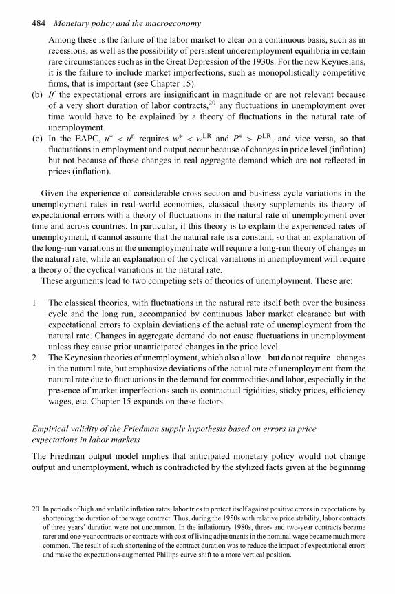
484 Monetary policy and the macroeconomy
Among these is the failure of the labor market to clear on a continuous basis, such as inrecessions, as well as the possibility of persistent underemployment equilibria in certainrare circumstances such as in the Great Depression of the 1930s. For the new Keynesians,it is the failure to include market imperfections, such as monopolistically competitivefirms, that is important (see Chapter 15).
(b) If the expectational errors are insignificant in magnitude or are not relevant becauseof a very short duration of labor contracts,20 any fluctuations in unemployment overtime would have to be explained by a theory of fluctuations in the natural rate ofunemployment.
(c) In the EAPC, u∗ < un requires w∗ < wLR and P∗ > PLR, and vice versa, so thatfluctuations in employment and output occur because of changes in price level (inflation)but not because of those changes in real aggregate demand which are not reflected inprices (inflation).
Given the experience of considerable cross section and business cycle variations in theunemployment rates in real-world economies, classical theory supplements its theory ofexpectational errors with a theory of fluctuations in the natural rate of unemployment overtime and across countries. In particular, if this theory is to explain the experienced rates ofunemployment, it cannot assume that the natural rate is a constant, so that an explanation ofthe long-run variations in the unemployment rate will require a long-run theory of changes inthe natural rate, while an explanation of the cyclical variations in unemployment will requirea theory of the cyclical variations in the natural rate.
These arguments lead to two competing sets of theories of unemployment. These are:
1 The classical theories, with fluctuations in the natural rate itself both over the businesscycle and the long run, accompanied by continuous labor market clearance but withexpectational errors to explain deviations of the actual rate of unemployment from thenatural rate. Changes in aggregate demand do not cause fluctuations in unemploymentunless they cause prior unanticipated changes in the price level.
2 The Keynesian theories of unemployment, which also allow – but do not require– changesin the natural rate, but emphasize deviations of the actual rate of unemployment from thenatural rate due to fluctuations in the demand for commodities and labor, especially in thepresence of market imperfections such as contractual rigidities, sticky prices, efficiencywages, etc. Chapter 15 expands on these factors.
Empirical validity of the Friedman supply hypothesis based on errors in priceexpectations in labor markets
The Friedman output model implies that anticipated monetary policy would not changeoutput and unemployment, which is contradicted by the stylized facts given at the beginning
20 In periods of high and volatile inflation rates, labor tries to protect itself against positive errors in expectations byshortening the duration of the wage contract. Thus, during the 1950s with relative price stability, labor contractsof three years’ duration were not uncommon. In the inflationary 1980s, three- and two-year contracts becamerarer and one-year contracts or contracts with cost of living adjustments in the nominal wage became much morecommon. The result of such shortening of the contract duration was to reduce the impact of expectational errorsand make the expectations-augmented Phillips curve shift to a more vertical position.

The classical paradigm 485
of this chapter. Further, the Friedman model asserts that the effects of monetary policychanges, both anticipated and unanticipated, must go through errors in the price expectationsembedded in wage contracts and a subsequent decrease in real wages. This too is contradictedby the stylized facts: an expansionary monetary policy increases output and reducesunemployment without necessarily producing a prior change in the price level or a decreasein real wages. Therefore, Friedman’s short-run model of commodity supply does notprovide a satisfactory explanation of the short-run impact of monetary policy on outputand unemployment.
14.11 Price expectations and commodity markets: the Lucas supplyfunction
The EAPC is based on the possibility that unanticipated price changes generate expec-tational errors in real wages in the labor market. This emphasis on the labor marketis in some ways more consistent with the Keynesian aggregative analysis, though theexpectations-augmented Phillips curve is associated with Milton Friedman. Neoclassicalanalysis focuses more on the markets for commodities and its microeconomic Walrasianbasis, as in Chapter 3, which implies that the output of each commodity depends uponits relative price. Lucas (1972, 1973) and Sargent and Wallace (1975) modified thecertainty version of the microeconomic model by introducing into it uncertainty and firms’expectations on relative product prices. This section presents one version of the Lucasanalysis.21
Lucas supply function or rule
Assume as in the preceding section that firm i produces good Xi, with the quantity produced asxi and sold at the price pi. The firm buys inputs, of which labor is taken to be the only variableinput. Given the nominal wage W , profit maximization by the firm in perfect competitionimplies that its supply function is given by:
xi = xi(pi/W ) xi′ > 0 (54)
with pi determined in the perfectly competitive market i. While the firm is not directlyconcerned with the price level P, Lucas’s analysis assumes that the nominal wages changeproportionately with the price level, so that P can be used as an index of labor cost.22
Therefore, replacing W by P,
xi = xi(pi/P) xi′ > 0 (55)
21 See Walsh (2003, Ch. 5) for another version of the Lucas model.22 For the price level to serve as an index of labor costs, the nominal wage rate must instantly adjust proportionately
to the actual price level. Hence, there must be nominal wage flexibility and instant adjustment in nominalwages, without any rigidities introduced by labor contracts or money illusion in the labor supply function.Compare this with the expectations-augmented Phillips’ curve, also in the neoclassical tradition, whichassumes that nominal wages do not rise proportionately with the actual price level but do so only withrespect to the expected price level, so that real wages do change because of the unanticipated part ofinflation.

486 Monetary policy and the macroeconomy
For simplification, Lucas assumes that the price pi in market i deviates in percentage termsfrom P by an amount zi which is normally distributed, independent of P and has a zeroexpected value and variance η2. Therefore,
pi = P + zi (56)
Hence, zi (= pi −P) defines the deviation of the i th product’s price from the price level. Theproduct price pi is called the “local price” while zi (= pi/P) is referred to as the “relativeprice,’ so that the change in the local price of the i th product incorporates changes in boththe price level and its relative price. Both increases in the general price level and in the firms’relative product price can occur at any time. The i th firm is assumed to know the price of itsown product but not to know the price level, which it estimates conditional on the informationavailable to it. Given such uncertainty, re-specify (55) as:
xit = xi(pit/E(Pet |It(i)) xi
′ > 0 (57)
where:xit = output in market i in period tE(Pe
t |It(i) = mean (mathematical expectation) of the price level expected for period tby firms in market i , conditional on It(i)
It(i) = information available in market i in period t.
Specify the log-linear form of (57) as:
xit = x∗it + γ [pit − E(Pe
t |It(i))] γ > 0 (58)
where all the variables are now in logs and x∗it is the i th firm’s output under perfect certainty
or if there are no expectational errors. γ is the firm’s response to an increase in its relativeprice.
Lucas (1972, 1973) provides a specific procedure for determining the expected relativeprices. Firms use the available information on aggregate demand and supply movements, andon local and general prices, to form their expectations on the distribution of local and generalprices in the present period.23 This provides them, at the beginning of the current period,with a prior distribution of the expected price level Pe, with mean P and constant varianceσ 2, with this distribution formed prior to the observation of the current local prices.24 Duringperiod t, the firm knows P, σ 2, η2 and observes pi. The (i th) firm uses this knowledge of itslocal price to calculate E(Pe
t |It(i)) as:
E(Pet |It(i)) = P t +[σ 2/(η2 +σ 2)][pit − P t] (59)
where:P t = mean of the prior distribution of expected pricesσ 2 = expected variance of P (“price level variability”)η2 = expected variance of zi (“relative price variability”)σ 2 +η2 = expected variance of pi (“local price variability”).
23 This would include knowledge of past shifts in demand and supply and past variations in local and generalprices, but can also include any available information about the future.
24 These assumptions make the deviation of the relative price a random one.

The classical paradigm 487
The second term on the right of (59) is the correction made to the prior expectation Pt ofthe price level on the basis of the observed local price pit .
Equation (59) was justified on the basis of information available in the i th market whenthe price level is not directly observed. This view of the nature of information was couchedby Lucas (1972) in what has come to be known as the island parable. This parable envisionsthe workers and firms as distributed spatially over islands (or isolated points). The firms donot know about activity (prices and output) on other islands but must forecast the averageprice level (over all the islands) in order to formulate their labor demand and output supplydecisions. To forecast the price level, they use the historic variability of their island price –represented by (η2 +σ 2) – relative to overall variability to forecast the shift of the price levelfrom a prior expected level, and do so as specified in (59).
Rewrite (59) as:
E(Pet |It(i)) = αPt + (1 −α)pit (60)
where α = η2/(η2 + σ 2) ≥ 0, so that α is the expected ratio of the relative price variance tothe total local price variance.
Substituting (60) in (58), we have:
xit = x∗it +αγ [pit − P t] (61)
Integrating (61) over all markets i, with total output supply designated as ys, and replacingthe known local price pit by the actual aggregate price level Pt ,
yst = y∗
t +αγ [Pt − P t] (62)
which is the aggregate supply function based on firms’ expectations about variations in localand general prices. The two components of a firm’s response to an expectation error are: (a) γ ,which is the change in output in response to the expectation error (P −Pe); and (b) α, whichis the revision of Pe from its prior value P. (62) is known as the Lucas supply function or rule.
If η = 0 and α = 0, so that relative prices are expected to be stable, (62) becomes:
yst = yf
t (63)
In this case with η = 0, aggregate supply will not respond to absolute price changes and henceto changes in aggregate demand, with the result that the aggregate supply function will bevertical in the (y, P) space. But if σ → 0 – that is, the price level is expected to be stable, sothat the change in local price is taken to be wholly a relative price change – the aggregatesupply function will become:
yst = y∗
t + γ [Pt − P t]
where γ is likely to be positive since it reflects firms’ responses to an increase in their relativeprices.
Another explanation of the Lucas supply function
Equation (62) was based on price misperceptions. It is to be distinguished from asomewhat similar equation, also attributed to Lucas, which can be derived from the

488 Monetary policy and the macroeconomy
intertemporal substitution of work in household decisions. In this model of intertemporalutility maximization, for given nominal wages in each period and a given current price levelPt , if the expected price level (Pe
t+1) rises, it will decrease the expected future real wage(we
t+1) for the given nominal wage,25 while the current real wage (wt) is unaffected. Hence,from utility optimization, workers will substitute work in the current period (i.e. increasens
t by decreasing their leisure time in t) for work in future periods (i.e. decrease nst+1 by
increasing leisure in t +1). Conversely, they would work – and produce – less in the presentperiod if, at the given current price level, the expected future price is lower and the expectedreal wage higher. Such behavior would produce recessions in output in the latter case andbooms in the former, thus causing real business cycles. However, the empirical significanceof such a model is limited since the observed intertemporal substitution of work in laborsupply decisions on the basis of price movements is too low to imply the larger observedvariations in output over the business cycle, so that we shall ignore it further in this chapter.
Comparing the Friedman and the Lucas supply functions
We are, therefore, left with two types of expectations-based Phillips curve relationships.One of these is Friedman’s expectations-augmented Phillips curve, which is based on errorsin expectations in labor market and contractual rigidities; and the other is Lucas’s supplyfunction, based on errors in the expectations of relative prices in commodity markets. Theformer is sometimes claimed to be an example of the latter under the argument that nominalwages are the “local” price of workers as suppliers of labor and the observed increases inthese nominal wages are used by the workers in forming their expectations on the price leveland the real wage (the “relative price” of labor). However, the theoretical and empirical basesof the two are quite different,26 so that it is preferable to keep them separate for analyticalreasons. But they are similar in spirit in that both maintain full employment unless there areerrors in expectations. Note that the errors in price expectations will be corrected as timepasses since this will provide information on the actual prices. In modern economies, thelag in information on actual prices and inflation rates is often a month or a few months,so that any expectational errors would be corrected fairly soon. Therefore, both the errorsin expectations and the deviation of short-run equilibrium output from the full-employmentoutput will be self-correcting and transient.
14.12 The Lucas model with supply and demand functions
The Lucas supply function derived above is:
yst = y∗
t +αγ [Pt − Pt] (62)
On the aggregate demand function, Lucas (1972, 1973) assumed that:
Y dt = Y d
t−1 + δ +μt (64)
25 Note that this assumption of the rigidity of the future nominal wage in the face of the expected rise in the pricelevel seems unrealistic.
26 In particular, the expectations-augmented Phillips curve requires contractual rigidities in nominal wages whilethe Lucas supply rule does not have such contractual rigidities. In the EAPC, if there is an unanticipated rise inprices, workers’ real wage falls, so that it is the workers who lose. In the Lucas model, the unanticipated rise inprices fools firms and their profits fall.
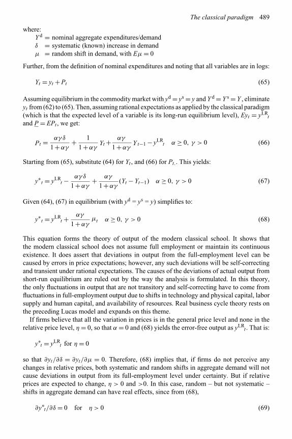
The classical paradigm 489
where:Y d = nominal aggregate expenditures/demandδ = systematic (known) increase in demandμ = random shift in demand, with Eμ = 0
Further, from the definition of nominal expenditures and noting that all variables are in logs:
Yt = yt + Pt (65)
Assuming equilibrium in the commodity market with yd = ys = y and Y d = Y s = Y , eliminateyt from (62) to (65). Then, assuming rational expectations as applied by the classical paradigm(which is that the expected level of a variable is its long-run equilibrium level), Eyt = yLR
t
and P = EPt , we get:
Pt = αγ δ
1 +αγ+ 1
1 +αγYt + αγ
1 +αγY t−1 − yLR
t α ≥ 0, γ > 0 (66)
Starting from (65), substitute (64) for Yt , and (66) for Pt.. This yields:
y∗t = yLR
t − αγ δ
1 +αγ+ αγ
1 +αγ(Yt − Yt−1) α ≥ 0, γ > 0 (67)
Given (64), (67) in equilibrium (with yd = ys = y) simplifies to:
y∗t = yLR
t + αγ
1 +αγμt α ≥ 0, γ > 0 (68)
This equation forms the theory of output of the modern classical school. It shows thatthe modern classical school does not assume full employment or maintain its continuousexistence. It does assert that deviations in output from the full-employment level can becaused by errors in price expectations; however, any such deviations will be self-correctingand transient under rational expectations. The causes of the deviations of actual output fromshort-run equilibrium are ruled out by the way the analysis is formulated. In this theory,the only fluctuations in output that are not transitory and self-correcting have to come fromfluctuations in full-employment output due to shifts in technology and physical capital, laborsupply and human capital, and availability of resources. Real business cycle theory rests onthe preceding Lucas model and expands on this theme.
If firms believe that all the variation in prices is in the general price level and none in therelative price level, η = 0, so that α = 0 and (68) yields the error-free output as yLR
t . That is:
y∗t = yLR
t for η = 0
so that ∂yt/∂δ = ∂yt/∂μ = 0. Therefore, (68) implies that, if firms do not perceive anychanges in relative prices, both systematic and random shifts in aggregate demand will notcause deviations in output from its full-employment level under certainty. But if relativeprices are expected to change, η > 0 and >0. In this case, random – but not systematic –shifts in aggregate demand can have real effects, since from (68),
∂y∗t/∂δ = 0 for η > 0 (69)

490 Monetary policy and the macroeconomy
while:
∂y∗t
∂μt= αγ
1 +αγ= η2 γ
σ 2 +η2(1 + γ )> 0 for η > 0 (70)
Note from (70) that even the random shifts in aggregate demand cause changes in outputonly if firms misinterpret its impact on the price level and believe that some part of theresulting increase in prices is a relative price increase. In conditions of hyperinflation wherethe likelihood and magnitude of general price increases dominate over relative price increases,the public’s expectation is likely to be η = 0, so that even random changes in aggregate demandwill not have any effects on output. In this context, neither systematic nor random demandincreases will change output. Therefore, for hyperinflations, money is likely to be neutral forboth systematic and random increases in the money supply. Hence, even random increasesin the money supply will not always induce increases in output and employment.
Asymmetric information and the impact of systematic demand increases on output
Equation (69) states that systematic demand increases by the policy makers will not changereal output. But, suppose that the policy makers systematically (for example, through the useof a rule such as the Taylor rule) increase demand but in such a way (as by a one-time shift inthe coefficients of the rule followed) that the firms interpret it to be a random increase. This isa case of asymmetric information between the policy maker and the public. This “disguisedor misinterpreted” nature of systematic demand increase will allow the policy maker toincrease real output through the “random multiplier” ∂y/∂μ, whose value is specified by (70).However, the systematic nature of the demand increase will, sooner or later, be observedby firms, leading to two types of change. One, firms will find it optimal to acquire betterinformation so that their likelihood of correctly perceiving a systematic demand increaseas being systematic – rather than erroneously as random – will increase. For this correctlyperceived systematic demand increase, there will be no change in output. Second, firms facedwith repeated increases in the general price level will modify their expectations on prices byincreasing the value of σ 2 relative to η2, so that ∂y/∂μ will decrease. In the limiting case,if there were only systematically induced increases in the price level, firms would adjust theirexpectations such that η2/(σ 2 + η2) → 0, so that ∂y/∂μ will go to zero. That is, systematicdemand increases, disguised or misinterpreted as being random ones, will eventually losetheir efficacy.
The implications of the Lucas model for unemployment
To examine the response of unemployment to changes in aggregate demand, start with thedefinition of unemployment as being (L − n) and use the production function y = y(n),y′(n) > 0, to go from y to u. Then, (68) implies that employment n is a function of the randomdemand term μt but not of the systematic demand term δ. With all variables being in logs,and assuming a log-linear relationship, (68) implies that:
u∗t = un −βμt β ≥ 0 (71)
where u∗ is the short-run equilibrium unemployment rate, β is a positive function of[αγ/(1 +αγ )] with β = 0 if α = 0. First note that δ is not in (71), just as it was not in

The classical paradigm 491
(68), so that ∂u∗t /∂δ = 0. Second, note that α is in (71) through β, just as it was in (68), and
that β > 0 for α > 0 and γ > 0. For β > 0, unemployment decreases if there is a randomincrease in aggregate demand, since the latter would persuade individual firms that the relativedemand and the relative price of their product have increased. That is, for β > 0, (71) impliesa negatively sloped curve in the (y, u) space, which looks like a Phillips curve – but is not thePhillips curve27 – and can be called the “Lucas–Phillips curve.” Hence, there is a seemingtradeoff – for given expectations on general versus relative price increases – between pricelevel increases and output increases in the short run.
However, there is a vital difference between (71) and the standard Phillips curve (forwhich, see Chapter 15). While the latter was envisaged by the Keynesians as a durabletradeoff between price increases (both anticipated and unanticipated) and unemployment,(71) cannot be used as a durable tradeoff for policy purposes. Meaningful policy increasesin demand cannot be random but must be systematic, such as by a constant δ in (64) aboveor according to some established rule, and, under the Lucas analysis, any systematic demandchanges cannot change real output. Further, as argued above, any systematic demand or priceincreases, disguised or misinterpreted as being random ones, will sooner or later lose theirefficacy as their systematic nature becomes understood.
Hence, according to (71), correctly anticipated inflation – such as would be the case ifthe inflation rate were constant or steadily increasing – has a vertical Lucas–Phillips curve,thereby not providing a durable impact of money, prices and inflation on output. This is nowgenerally accepted. However, it is now also accepted that in the short run, monetary policy,whether operating through money supply or interest rates, does affect output and does soearlier than prices and inflation, as indicated in the stylized facts at the beginning of thischapter. It is now generally accepted that these facts cannot be explained in a satisfactorymanner by imperfect information, resulting in temporary price or inflation misperceptions,but must rest on theoretical foundations and empirical factors not encompassed in Lucas’sanalysis.
Empirical validity of the Lucas supply model based on price misperceptionsin the commodity market
The Lucas output model (Lucas, 1972, 1973; Sargent and Wallace, 1976; see alsoChapter 17) implies that anticipated monetary policy would not change output andunemployment. This clearly contradicts the stylized facts given at the beginning of thischapter. Further, the Lucas model asserts that the effects of monetary policy changes, bothanticipated and unanticipated, must go through price level changes and errors in priceexpectations. This too is contradicted by the stylized facts: an expansionary monetarypolicy increases output and reduces unemployment without necessarily producing a priorchange in the price level, as Lucas (1996) concluded later from his assessment of theempirical evidence (see Section 14.16). Therefore, for the short run, the Lucas model does
27 It is not the Phillips curve or the EAPC because these are based on real wages actually falling as inflation occurs,while the Lucas version does not allow this fall. His curve emanates from the firm’s belief that relative pricesare increasing when they are not, so that the perceived inflation rate is below the actual one. Since, under ourassumptions, nominal wages increase proportionately with the actual rate of inflation, the firm’s relative pricemisperceptions imply that the firm’s perception is that the real wage is falling, even though it does not do so.This has the consequence that the firm’s real profits fall even as it supplies more output – so that its outputincrease is likely to be short lived.

492 Monetary policy and the macroeconomy
not provide a satisfactory explanation of the impact of monetary policy on output andunemployment.
14.13 Defining and demarcating the models of the classical paradigm
Evolution of the classical paradigm
The principles of the classical paradigm evolved out of several rather disparate elements. Thedominant one was the economic and political philosophy of liberalism in the first half of thenineteenth century. Its economic analysis was that of individual markets for commodities,factors of production, money and bonds, with competition as the invisible hand guidingeach of them to equilibrium through the adjustment of the relevant price. In this analysis,all prices were flexible and adjusted to bring each market into equilibrium, so that eachmarket cleared at the trading price. Much of this analysis of individual markets was setout in the following rather separate categories: individual commodity and labor markets todetermine relative prices, wages, output and employment; quantity theory for determiningthe price level and the loanable funds theory for determining the interest rate; and businesscycle theories. These distinctive theories nowhere appeared in an integrated format so that onecannot point to the work of any economist prior to Keynes’s book The General Theory (1936)for a statement of an integrated macroeconomic theory or model. In particular, there was nointegrated model that included the consumption and saving functions and the investmentmultiplier, and therefore, no aggregative theory of the commodity market. Further, whilethere was a great deal of discussion about the nature of risk and uncertainty, the abovecomponents of the traditional classical approach did not incorporate it in a meaningfulway. These are the elements of what Keynes labeled in Chapter 1 of The General Theoryas the classical model, though there did not exist in the literature at that time such anestablished and complete macroeconomic model. We have labeled this pre-Keynesian modelthe traditional classical model, in comparison with the subsequent neoclassical and modernclassical models.
Keynes’s The General Theory for the first time provided an integrated macro modelof the economy and also fundamentally altered the way the profession models short-runaggregative economics. He chose to give the foremost place in his model to the commoditymarket, with an analysis incorporating the multiplier and also money demand analysis. JohnHicks (1937) organized Keynes’s ideas on the commodity and monetary sectors into what helabeled the IS–LM framework, and cast the traditional classical model in the same format tofacilitate comparison. The traditional classical model thus recast in the mould of the IS–LMframework, which had been proposed to illuminate Keynes’s ideas, came to be known asthe neoclassical model. The IS–LM model of aggregate demand, combined with the AD–ASmodel for the determination of output and the price level, provided the first formally integratedmacroeconomic model of the classical paradigm. It was elaborated and refined in the decadesup to 1970.
Neoclassical economics with the addition of rational expectations, if there is uncertainty,and an insistence on continuous labor market clearance has been labeled in this book themodern classical model.28 The combination of the modern classical model with Ricardian
28 Note there are many significant differences between the somewhat diffuse ideas of the nineteenth century andthe modern classical model. Among these differences is the explicit commodity market analysis incorporating

The classical paradigm 493
equivalence has been labeled the new classical model. In general, these models of the classicalparadigm do not incorporate market imperfections, that is, deviations from the perfect marketsassumption, which are emphasized in Keynesian economics (see next chapter).
There can be considerable disputes about the proper delineation of the classical schoolsor models. We introduced the following taxonomy in Chapter 1. We elaborate on it here,though at the risk of some repetition. No claim is being made to this taxonomy being auniversal – or perhaps even a majority – one. We have chosen it below for reasons of clarityin separating each model from the others, rather than leaving their differences ambiguous,while maintaining consistency with the writings and folklore in the history of economicsthought.
All the schools of the classical paradigm share the common belief that the real-worldeconomy under consideration – and not just the models – functions at full employment in thelong run and that one of the characteristics of long-run equilibrium is the independence of thereal variables from the financial ones, so that money is neutral in the such equilibrium. Further,all schools share the belief that deviations from the long-run equilibrium can occur in the shortrun but such deviations are self-correcting and transient. States with less than full employmentare, therefore, states of disequilibrium during which the economy continues to adjust towardsits full-employment equilibrium – and not away from it, A major difference among theseschools is whether the real-world economy adjusts so fast as to have continuous equilibrium,so that it will not show any evidence of disequilibrium, even though disequilibrium remainsa hypothetical state within the model.
The traditional (pre-Keynesian) classical ideas
This section lays out our interpretation and distillation of the writings of the pre-Keynesianeconomists. Their ideas were not expressed or formulated in terms of a compact model, andthe analysis of the expenditure sector (the IS curve) and the multiplier was not available tothem. Their common belief was that output and employment in the long run equilibriumdepended upon the real sector’s relationships only and were independent of the monetarysector. The economy’s interest rate was determined by the theory of loanable funds, whichin modern terminology corresponds to the market for bonds (see Chapter 19). Further, thequantity theory for the determination of the price level applied in equilibrium. But outsidethis equilibrium, changes in the money supply could change output and employment. Notonly could the money supply affect the real sector in this way, the economy was consideredto be very prone to fluctuations in output and employment. Many of these fluctuations wereattributed to money supply shocks or the response of the money supply to real shocks.In particular, most of the classical economists did not believe that the economy functionedso well that it always maintained full employment or that it did so most of the time.In fact, recessions and crises – many of them originating in the banking sector or financialspeculation or occurring due to the response pattern of the financial sector to real shocks –were common, and widely recognized as such, during the nineteenth century. Hence, thetraditional classical school did not assume continuous full employment or that it existed mostof the time.
the multiplier concept, the interest sensitivity of money demand, the elimination of the direct transmissionmechanism of money supply effects on nominal income, explicit analysis of government deficits and theirimplied future taxes, rational expectations, etc.

494 Monetary policy and the macroeconomy
The neoclassical model
This model was an attempt to bottle the main ideas of the pre-Keynesian classicaleconomists into a compact modern macroeconomic model. This process was initiated byHicks in 1937, who borrowed the IS–LM analysis from Keynes’s work and used it as atechnique for interpreting the traditional classical ideas, thereby re-incarnating those ideasinto the neoclassical model. The neoclassical model continued to have both equilibriumand disequilibrium aspects and did not assume instantaneous market clearance. In this, itrepresents the ideas of the pre-Keynesian classical economists more faithfully than does themodern classical model.29
The modern classical and new classical models
The certainty version of the modern classical model modifies the neoclassical model byadding the assumption of continuous market clearance, especially of the labor market at thefull-employment level. By doing so, it ignores the disequilibrium properties and multipliersof the neoclassical model as being irrelevant in practice. The uncertainty version of this modeladds in the rational expectations hypothesis. Some economists would also add to this mix theassumption of Ricardian equivalence. However, our definition of the modern classical modelexcludes this assumption, only making it part of the new classical model. This differentiationmeans that, under our definitions, fiscal policy would change aggregate demand in the modernclassical model but not in the new classical model.
Hence, under our designations, the constituents of the modern classical model are:
1 the neoclassical model, modified by the additions of:2 uncertainty, with deviations of output and employment from their long-run values due to
errors in price expectations;3 the rational expectations hypothesis, which implies that the errors in expectations will
be random;4 continuous market clearance (especially of the commodity and labor markets).
The constituents of the new classical model are:
1 the modern classical model, modified by the addition of:2 Ricardian equivalence.
Note that both the modern classical and the new classical models do possess money supplychanges as a policy tool for changing aggregate demand in the economy, but, of the two,only the modern classical model allows fiscal policy to change aggregate demand. For thelong run, both these models imply the neutrality of money in the full-employment state, sothat the impact of the money supply and velocity changes can only be on the price leveland not on real output and employment. Further, for the short run, unanticipated changesin money supply and velocity can cause deviations of short-run output and employment
29 This modern classical model is also different from the traditional classical model in other ways. One of theserelates to the existence of speculative balances in the modern classical model, whereas the quantity theorycomponent of the traditional classical model did not have such balances.

The classical paradigm 495
from their long-run values, but, given rational expectations, these deviations will be transientand self-correcting as new information on prices becomes available. Therefore, both themodern classical and the new classical models imply that there is neither a need nor scopefor systematic monetary policy for changing the levels of output and employment in theeconomy, so that such policies should not be pursued. These ideas are further explored inChapters 15 and 17.
14.14 Real business cycle theory and monetary policy
Business cycles are cyclical fluctuations in the economy’s output and employment in real, notanalytical, time. Their explanation relates to the short term, which is a chronological conceptof time, rather than the analytical short run or long run.
Real business cycle theory is an offshoot of the modern classical model and asserts thatbusiness fluctuations occur only in response to shocks to the fundamental determinants oflong-run output and employment (e.g. see Prescott, 1986; Christiano and Eichenbaum, 1992;Romer, 1996, Ch. 4). These determinants are technology, which determines the productionfunction and the demand for inputs, and the supply of factor inputs. Among the determinantsof the latter are preferences, including those on labor supply, which depends on the labor–leisure choice and the stock of resources. Shifts in the production function or input suppliesalter long-run equilibrium output, as well as being a source of cyclical fluctuations in output.The real business cycle theory derives the fundamental determinants of business cycles fromthe general macroeconomic models of the classical paradigm.
Explicitly, or by omission, real business cycle theory also holds that shifts in aggregatedemand, no matter what their source, do not cause changes in output and employmentand therefore do not cause business cycle fluctuations. Therefore, changes in consumption,investment, exports, money supply and demand (or the central bank’s interest rate policy) orfiscal deficits cannot change output and employment. This exclusionary proposition is derivedfrom the properties of the long-run equilibrium of the modern classical model. To be valid,it requires perfectly competitive markets and also that long-run equilibrium is continuouslymaintained in the economy.
The policy implication of real business cycle theory, as of the modern classical modelof which it is an elaboration, is that systematic monetary (and fiscal) policies cannot affectoutput and employment, so that they cannot be used to moderate the business cycle. Thecritical elements for this implication are the Friedman–Lucas supply equation and rationalexpectations, according to which anticipated changes in prices, inflation and monetary policycannot affect output. Therefore, the Taylor rule, under which systematic monetary policymanipulates aggregate demand by changing the interest rate in response to the output gapand the deviation of inflation from its target rate, can only be useful in controlling inflation butnot in moderating the output gap. According to the modern classical school, while randommonetary policy can change aggregate demand, the central bank cannot predict and thereforecannot offset the random fluctuations in the private components of aggregate demand. In short,in the new classical model, monetary policy and the Taylor rule have no legitimate role inmoderating or reducing the duration of business cycles.
Intuitively, the problem with the real business cycle theory is most evident in its explanationof recessions. It attributes recessions to a fall in labor productivity and/or an increase in thepreference for leisure. The objections to these explanations are succinctly stated by the quip:recessions occur because “workers forget how to do things” (“lose some of their knowledge”)and/or because they decide to become lazier for some time, thereby causing the recessionary

496 Monetary policy and the macroeconomy
fall in output! Neither of these explanations is plausible, so the validity of the real businesscycle theory is highly doubtful. Looking at upturns in business cycles, the real business cycletheory attributes upturns to increases in productivity and/or increases in the preference forwork over leisure. The latter is hardly plausible over the length of upturns in the economy,while the former is highly plausible. Here, however, it is the plausibility of the assertion ofreal business cycle theory that aggregate demand increases cannot also be a source of upturnsthat is highly doubtful.
The real business cycle propositions rest on the assumption that all markets can be taken tobe competitive and efficient (i.e. continuous equilibrium) in the economy. This assumptionis not consistent with models of the Keynesian paradigm, since they incorporate marketimperfections and/or failure of the economy to achieve long-run equilibrium instantly aftera demand shock. In these models, shifts in aggregate demand, whether through shifts ininvestment and other private sector variables or in monetary and fiscal policy, can producechanges in output and be a source of, or contribute to the continuation of, business cycles. Morespecifically on monetary policy, market imperfections can create non-neutrality of money,so that fluctuations in the money supply can add to output fluctuations. Conversely, theappropriate monetary policy can reduce the severity of cyclical fluctuations due to aggregatedemand shocks coming from the private sector. Further, Keynesians do not deny that shifts inthe fundamental determinants of output, mentioned above, can also cause output fluctuations.
Therefore, the core of the debate about the validity of real business cycle theory is not aboutwhether shocks to technology and factor inputs can cause cyclical fluctuations, for that is not indispute. It is rather about whether shocks to aggregate demand can cause such fluctuations andwhether monetary policy can moderate them. Real business cycles and the modern classicalschool deny that they can, or do so in a significant manner, while Keynesians assert that theycan do so. This issue is easily testable by the appropriate causality tests. The consensus on theempirical evidence seems to be that the major part (in some estimates, as large as 70 percent)of the fluctuations in output can be attributed to productivity shocks. This is a testament to thesuccess of real business cycle theory, as compared with Keynesian ideas from the 1940s tothe 1970s that had attributed most business cycle fluctuations to shifts in aggregate demand.However, the empirical evidence leaves a very significant part of the fluctuations in output thatcannot be explained by shifts in technology and preferences. Overall, the empirical evidence,as well as intuition, seems to indicate that fluctuations in aggregate demand, in addition tochanges in technology and preferences, do cause fluctuations in output and employment andthat money supply growth is positively related to output growth. Therefore, real businesscycle theory is not strictly valid, and monetary policy can be pursued in appropriate cases toreduce output fluctuations.
The exponents of the real business cycle theory also prefer to test this theory bythe calibration and simulation of models rather than by the econometric testing of theirhypotheses. The former procedure requires a priori specification of the likely values of theparameters, on which there can be considerable doubts. Further, the findings may not be robustto small changes in these assumed values, or consistency with the empirical observations mayrequire implausible values. Consequently, this testing procedure and its reported findings havenot won general acceptance.
There seem to be at least two major contributions of the real business cycle theory.One, it has firmly established that changes in technology and preferences do cause cyclicalfluctuations in output and may do so significantly more than fluctuations in aggregatedemand. Two, the approach initiated by the real business cycle agenda to macroeconomicmodeling is now firmly established. This approach requires that macroeconomics be based on

The classical paradigm 497
optimization over time by individual economic agents in a dynamic context. This stochasticdynamic intertemporal approach to macroeconomics permeates current macroeconomicmodels, including the new Keynesian model, which is presented in the next chapter. Themajor deficiency and unrealistic assertion of the real business cycle theory is that it deniesdemand shifts any role in output fluctuations.
The empirical evidence on the impact of changes in aggregate demand on output is oftenon the impact of money supply changes, which change aggregate demand, on output. Theinfluential study by Friedman and Schwartz (1963a,b) used evidence from over 100 yearsof US data to show clear evidence that money supply changes lead, and therefore Granger-cause, changes in real economic activity. However, inside money (i.e. deposits in banks)is the largest component of money. Subsequent contributions by other authors showed thatdeposits respond to macroeconomic disturbances, so that money is more highly correlatedwith lagged output than with future output; i.e. deposits lag rather than lead output. However,monetary aggregates such as M2 still lead output. Further, if the central bank uses the interestrate as its operating monetary policy target, and money supply responds endogenously to it,the evidence seems to show that changes in interest rates lead output.
To conclude, empirical evidence shows that while shocks to real factors such as technologyand preferences do cause fluctuations in output, shocks to monetary policy variables of moneyand interest rates also do so. Models of the modern classical school and real business cycletheory do not provide a satisfactory explanation for the latter finding. In recent years, stickyprice and inflation models of the new Keynesian school have been proposed to explaineconomic fluctuations. An example of these studies is provided by Ireland (2001b).
14.15 Milton Friedman and monetarism
Milton Friedman occupies a special place in the counter-reformation from Keynesianeconomics to the neoclassical and eventually to the modern classical theories, though hisideas are, in many ways, closer to the neoclassical economics of the 1960s and 1970s thanto the modern thinking. In the 1950s, Friedman argued and showed through his theoreticaland empirical contributions that “money matters” – that is, changes in the money supplychange both nominal and real output – is against the then general view of the Keynesians thatchanges in the money supply brought about through monetary policy did not significantlyaffect the economy, or did so unpredictably.30 He argued and tried to establish throughempirical studies that, as far as nominal national income was concerned, the money-incomemultiplier was more stable than the investment-income multiplier, so that monetary policywas more predictable than fiscal policy in its impact on nominal national income. However,Friedman held that major instability in the US economy had been produced or, at the veryleast, greatly intensified by monetary instability and that major depressions were associatedwith monetary contractions, prior to and after the establishment of the Federal Reserve Systemin 1913. Therefore:
The first and most important lesson that history teaches about what monetary policycan do … is that monetary policy can prevent itself from being a major source ofeconomic disturbance. [However, while] monetary policy can contribute to offsettingmajor disturbances in the economic system arising from other sources … we simply
30 See Chapter 2 for the elucidation of his 1956 article.
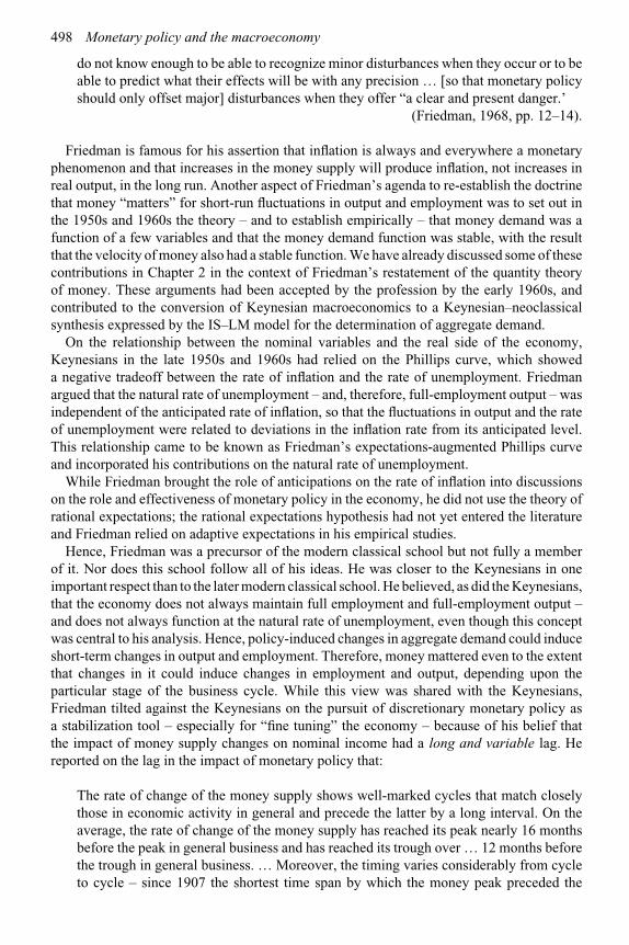
498 Monetary policy and the macroeconomy
do not know enough to be able to recognize minor disturbances when they occur or to beable to predict what their effects will be with any precision … [so that monetary policyshould only offset major] disturbances when they offer “a clear and present danger.’
(Friedman, 1968, pp. 12–14).
Friedman is famous for his assertion that inflation is always and everywhere a monetaryphenomenon and that increases in the money supply will produce inflation, not increases inreal output, in the long run. Another aspect of Friedman’s agenda to re-establish the doctrinethat money “matters” for short-run fluctuations in output and employment was to set out inthe 1950s and 1960s the theory – and to establish empirically – that money demand was afunction of a few variables and that the money demand function was stable, with the resultthat the velocity of money also had a stable function. We have already discussed some of thesecontributions in Chapter 2 in the context of Friedman’s restatement of the quantity theoryof money. These arguments had been accepted by the profession by the early 1960s, andcontributed to the conversion of Keynesian macroeconomics to a Keynesian–neoclassicalsynthesis expressed by the IS–LM model for the determination of aggregate demand.
On the relationship between the nominal variables and the real side of the economy,Keynesians in the late 1950s and 1960s had relied on the Phillips curve, which showeda negative tradeoff between the rate of inflation and the rate of unemployment. Friedmanargued that the natural rate of unemployment – and, therefore, full-employment output – wasindependent of the anticipated rate of inflation, so that the fluctuations in output and the rateof unemployment were related to deviations in the inflation rate from its anticipated level.This relationship came to be known as Friedman’s expectations-augmented Phillips curveand incorporated his contributions on the natural rate of unemployment.
While Friedman brought the role of anticipations on the rate of inflation into discussionson the role and effectiveness of monetary policy in the economy, he did not use the theory ofrational expectations; the rational expectations hypothesis had not yet entered the literatureand Friedman relied on adaptive expectations in his empirical studies.
Hence, Friedman was a precursor of the modern classical school but not fully a memberof it. Nor does this school follow all of his ideas. He was closer to the Keynesians in oneimportant respect than to the later modern classical school. He believed, as did the Keynesians,that the economy does not always maintain full employment and full-employment output –and does not always function at the natural rate of unemployment, even though this conceptwas central to his analysis. Hence, policy-induced changes in aggregate demand could induceshort-term changes in output and employment. Therefore, money mattered even to the extentthat changes in it could induce changes in employment and output, depending upon theparticular stage of the business cycle. While this view was shared with the Keynesians,Friedman tilted against the Keynesians on the pursuit of discretionary monetary policy asa stabilization tool – especially for “fine tuning” the economy – because of his belief thatthe impact of money supply changes on nominal income had a long and variable lag. Hereported on the lag in the impact of monetary policy that:
The rate of change of the money supply shows well-marked cycles that match closelythose in economic activity in general and precede the latter by a long interval. On theaverage, the rate of change of the money supply has reached its peak nearly 16 monthsbefore the peak in general business and has reached its trough over … 12 months beforethe trough in general business. … Moreover, the timing varies considerably from cycleto cycle – since 1907 the shortest time span by which the money peak preceded the

The classical paradigm 499
business peak was 13 months, the longest 24 months; the corresponding range at troughsis 5 months to 21 months.
(Friedman, 1958; see Friedman, 1969, p. 180).
With such a long and variable lag between changes in the money supply and nominalincome, the monetary authorities cannot be sure when a policy-induced increase in the moneysupply would have its impact on the economy. Such an increase in a recession may not,in fact, increase aggregate demand until the following boom, thereby only increasing therate of inflation at that time. Consequently, Friedman argued that discretionary monetarypolicy, intended to stabilize the economy, could turn out to be destabilizing. Friedman’srecommendation on monetary policy was, therefore, that it should maintain a low constantrate of growth, as stated by him in:
There is little to be said in theory for the rule that the money supply should grow ata constant rate. The case for it is entirely that it would work in practice. There arepersuasive theoretical grounds for desiring to vary the rate of growth to offset otherfactors. The difficulty is that, in practice, we do not know when to do so and by howmuch. In practice, therefore, deviations from the simple rule have been destabilizingrather than the reverse.
(Friedman, 1959).31
Therefore, while both Friedman and the modern classical economists are opposed to thepursuit of discretionary monetary policy, they arrive at this position for quite different reasons.For Friedman, money supply changes can change output and employment but the long andvariable lags in this impact make a discretionary policy inadvisable; over time; it couldmake the economy perform worse rather than better. For the modern classical economists,the economy maintains full employment except for transitory and self-correcting deviationsfrom it due to random errors in price expectations, so that systematic policy changes in themoney supply cannot change output and employment, but only the price level. Further, forthis school, the lags in the impact of systematic money supply changes on nominal nationalincome are not significant.
On the transmission mechanism from money supply changes to income changes, Friedmansupported Fisher’s direct transmission mechanism (from money supply changes directly toexpenditures) over the indirect one (from money supply to interest rates to investment in theKeynesian and IS–LM models). Neoclassical and modern classical models espouse the latterrather than the former.
Monetarists and the St Louis equation
Monetarism and monetarists have been defined in a variety of ways. In a very broadsense, monetarism is the proposition that “money matters” in the economy. In this sense,Friedman, Keynes and the Keynesians32 were all monetarists, while the modern classical
31 The above prescriptions for policy were repeated in Friedman (1968).32 This was not true of many Keynesian models popular in the 1950s and 1960s. Some of these relegated money to a
minor role, since they claimed that money was only a small part of the economy’s liquidity, which included tradecredit, etc. Other models claimed that the price level and the inflation rate were an outcome of the struggle between

500 Monetary policy and the macroeconomy
school is less monetarist since it downplays the impact of money supply changes on thereal variables of the economy. In a narrow sense, monetarism as a label was associatedwith the St Louis school in monetary and macroeconomics. We shall define monetarismin this narrow sense. The St Louis school provided in the late 1960s and early 1970s anempirical procedure for estimating the relationship between nominal income and the moneysupply. This was the estimation of a reduced-form equation (Andersen and Jordan, 1968) ofthe form:
Yt = α0 +�iaiMt−i +�jbjGt−j +�scsZt−s +μt (72)
where:Y = nominal national incomeM = nominal value of the appropriate monetary aggregateG = value of the appropriate fiscal variablesZ = vector of the other independent variablesμ = disturbance term.
Equation (72) is called the St Louis monetarist equation and was presented earlierin Chapter 8. While its common form used nominal income as the dependent variable,the dependent variable can be changed, depending upon the researcher’s interest, to realoutput, the unemployment rate, the rate of inflation or some other endogenous variable.In general, the St Louis equation is a reduced-form estimation equation of the short-run macro models, with the monetary aggregates and the fiscal variables being taken asexogenous.
The St Louis equation has become a popular method for determining the impact of monetaryand fiscal policies on nominal national income and other variables. Its initial estimation byresearchers at the Federal Reserve Bank of St Louis (Andersen and Jordan, 1968) showed thatthe money aggregates had a strong, positive and rapid impact on nominal income, this impactbeing more significant than that of fiscal policy. The marginal money-income multiplierwas about 5 over five quarters, while the marginal impact of fiscal policy was positivefor the first year and then turned negative, with a multiplier of only about 0.05 over fivequarters.33 These findings were consistent with Friedman’s stance, except that the estimationsof the St Louis equation indicated a much shorter and more reliable lag than Friedman hadfound. Therefore, contrary to Friedman’s recommendations and consistent with those of theKeynesians, monetarism was consistent with the stance that monetary policy could be usefulfor short-term stabilization.
The St Louis monetarism represented a transitional stage in the transition from Keynesianascendancy in economics in the decades before 1970 to the ascendancy of the neoclassicaland modern classical schools in the 1980s and 1990s. In many ways, it was an amalgam ofKeynesian and Friedman’s ideas in macroeconomics, and led the way to the re-emergenceof the classical doctrines. While its theoretical underpinnings have not survived, its impact
firms and unions over relative income shares. Still others claimed that firms followed a full-cost pricing policy,with the money supply accommodating itself to the resulting price level because the central bank did not wantthe unemployment rate to rise.
33 Numerous applications of the St Louis equation showed that its empirical findings differed among countries,periods and the definitions of the policy variables. However, their basic conclusion, that money supply changeshave a strong short-term impact on the economy, remained fairly robust.

The classical paradigm 501
on monetary policy has proved to be longer lasting. On this, its contributions were thatmoney matters, that the control of the money supply is important for containing inflation andthat the responsibility for inflation rests with the central bank.
14.16 Empirical evidence
One way of assessing the empirical validity of the implications of the classical models isby comparing their implications with the stylized facts set out early in this chapter. Forthe long run, the classical models imply that output and unemployment in the economy areindependent of the money supply, price level and inflation, while the relationship betweenmoney supply and price level is proportionate. Both implications seem to be confirmed by dataover long periods of time (Kormendi and Meguire, 1984; Geweke, 1986; McCandless andWeber, 1995; Taylor, 1996; Lucas, 1996), though some studies show a positive correlationbetween output and inflation in a general context of low inflation (McCandless and Weber,1995) while others show a negative one, especially at higher inflation rates (Barro, 1996).
On the short-run or dynamic impact of an expansionary monetary policy, i.e. anexpansionary money supply and/or decrease in interest rates, the modern classical modelimplies, through the Friedman–Lucas supply analysis, that prices and inflation will increase.If the increase is unanticipated, output will rise and unemployment will fall; if it is anticipated,there will be no change in output and unemployment. However, as the stylized facts show, thedynamic response of output and unemployment to an expansionary monetary policy is hump-shaped: output first increases (and unemployment falls) for several quarters, and then beginsto decrease (Sims, 1992; Ball, 1993). This evidence contradicts the response pattern impliedby the modern classical school. Further, while the impacts of anticipated and unanticipatedmonetary policy can sometimes be different, this difference is not always significant. In anycase, an anticipated monetary policy usually does have a significant impact on output andunemployment, and unexpected price and inflation changes explain only a small fraction ofthe output changes that occur. Further, the real effects of monetary policy do not proceedthrough prior changes in prices and inflation rates, as asserted in the Friedman and Lucassupply rules (Lucas, 1996).
Therefore, the inescapable conclusion is that while the modern classical model does providean acceptable long-run relationship between money and output/unemployment (i.e. moneyand monetary policy are neutral), it does not provide a satisfactory short-run theory of theimpact of money and monetary policy on output and unemployment.
This chapter has presented the analyses of the classical paradigm in short-run macroeco-nomics. How does it perform empirically? For this, we rely on the assessment provided byRobert E. Lucas, who is associated with the modern classical school and has been a majorcontributor to it.
Lucas on the neutrality versus non-neutrality of money
In the “Nobel lecture” (1996), given on his receipt of the Nobel Prize in economics, RobertLucas noted that:
In summary, the prediction that prices respond proportionately to changes in the long-run,deduced by Hume in 1752 (and by many other theorists, by many different routes, since),has received ample – I would say decisive – confirmation, in data from many times andplaces….

502 Monetary policy and the macroeconomy
The observation that money changes induce output changes in the same directionreceives confirmation in some data sets but is hard to see in others. Large-scale reductionsin money growth can be associated with large-scale depressions or, if carried out in theform of a credible reform, with no depression at all.
(Lucas, 1996, p. 668; italics added).
Sometimes, as in the U.S. Great Depression, reductions in money growth seem to havelarge effects on production and employment. Other times, as in the ends of the post-WorldWar I European hyperinflations, large reductions in money growth seem to have beenneutral, or nearly so. Observations like these seem to imply that a theoretical frameworksuch as the Keynes–Hicks–Modigliani IS/LM model, in which a single multiplier isapplied to all money movements regardless of their source or predictability, is inadequatefor practical purposes.
(Lucas, 1994, p. 153; italics added).
Note that this quote states that changes in the money supply need not always be neutral andcan (not must) have large real effects, lasting over a considerable period. But the modernversions of the classical paradigm do not provide a theory to explain such significant instancesof the non-neutrality of money.
Lucas on the validity of the modern classical analysis for the short run
Lucas claims that “Macroeconomic models with realistic kinds of monetary non-neutralitiesdo not yet exist.” (Lucas, 1994, pp. 153–4). “… anticipated and unanticipated changes inmoney growth have very different effects” (1996, p. 679). However, on the models thatattribute this non-neutrality to unanticipated or random changes in the price level, the evidenceshows that:
Only small fractions of output variability can be accounted for by unexpected pricemovements. Though the evidence seems to show that monetary surprises have real effects,they do not seem to be transmitted through price increases, as in Lucas (1972).
(Lucas, 1996, p. 679; italics added).
Note that this quote indicates that money supply changes do not have to first causechanges in prices before they affect real output. That is, output may change in response tomonetary policy changes, even though the markets might not first or ever adjust prices. Thisimplies that an expansionary monetary policy would produce output increases before beingreflected in inflation (Mankiw, 2001). This is a powerful indictment of the long-run classicalparadigm with its underlying assumption at both the microeconomic and macroeconomicslevels, which is that following an increase in demand, prices are first adjusted by markets,and this is followed by adjustments in quantities demanded and supplied by economicagents.
Lucas on the state of macroeconomic theory
Little can be said to be firmly established about the importance and nature of the realeffects of monetary instability, at least for the U.S. in the postwar period. Though it iswidely agreed that we need economic theories that capture the non-neutral effects of

The classical paradigm 503
money in an accurate and operational way, none of the many available candidates iswithout serious difficulties.
(Lucas, 1994, p. 153; italics added).
Hence, given the above assessment by Lucas, it is fair to conclude that the short-runmodern classical models, based on his model of price misperceptions in the commoditymarket and/or on Friedman’s errors in expectations occurring in wage contracts, fail toprovide a satisfactory explanation of the empirical evidence on the impact of monetarypolicy on output, employment and unemployment. We must therefore continue the searchfor additional theories of such impact. The next chapter looks at various theories in theKeynesian paradigm, and their success in this objective.
Conclusions
The traditional classical model, dominant through most of the nineteenth and early twentiethcenturies, was a somewhat disorganized set of ideas, for which we can envisage fullemployment as the long-run equilibrium state but with the existence of disequilibriumbeing a distinct possibility. Changes in the money supply affected employment and outputand caused business cycle fluctuations. The main components of the traditional classicalanalysis were the quantity theory of prices and the theory of the rate of interest. Therewas no specific theory of employment and output, though there was a general belief that,after a monetary disturbance, the economy eventually returns to its full-employment level.There was also no treatment of the product market with its concept of the investmentmultiplier.
The neoclassical model reorganized the traditional classical analysis into a compact form,based on the IS–LM apparatus, and explicitly incorporated into it the analysis of the productmarket through the IS curve. It also replaced the quantity theory by a general equilibriumdetermination of the price level. In a departure from many other treatments of the neoclassicalmodel, our version, presented in this chapter, emphasizes both its equilibrium – at thefull-employment level – and disequilibrium analyses. In particular, it does not assumethat the latter can be ignored for applications to real-world economies and in its policyrecommendations.
In our definitions of the various schools that have evolved out of the neoclassical school,the addition of the assumptions of rational expectations and continuous equilibrium to theneoclassical model turns it into the modern classical model, which allows for short-rundeviations from full employment due to errors in expectations. Adding further the doctrineof Ricardian equivalence to the modern classical model defines the new classical model. Thislatter model implies that fiscal deficits do not even affect the commodity market equilibriumor aggregate demand in the economy, so that the fiscal variables cannot be used as a policytool. However, the money supply remains a policy tool for changing aggregate demand inthe economy.
The implications drawn from the neoclassical model are usually for its full-employmentequilibrium states. For such states, output is also at the full-employment level. Further, sincethe neoclassical economists usually assume that equilibrium is restored within a reasonableor acceptable period of time, the neoclassical prescription is that the economy should beleft alone to achieve equilibrium. Monetary and fiscal policies should not be pursued. Ifpursued, they cannot affect the equilibrium real values of the macroeconomic variables, butwould only change the nominal values. Few economists and central banks accept these

504 Monetary policy and the macroeconomy
propositions for the short-run impact of monetary and fiscal policies. Most, if not all,central banks actively pursue monetary policies to modify the short-run performance ofthe economy.
Versions of the equilibrium part of the neoclassical model provided, in the past, thetheoretical basis for the schools in political economy known as Reaganomics in the USAand Thatcherism in Britain. These philosophies of political economy advocated the cessationof any attempts by the monetary and fiscal authorities to change real output and employmentin the economy, and the restriction of monetary policy solely to the goal of price stabilization.These schools are no longer popular.
The short-run version of the modern classical model, in which deviations of output fromthe full-employment level occur through errors in expectations due to unanticipated priceinflation, is clearly not valid. This is clearly so, as a comparison of this model’s implicationwith the stylized facts on the impact of anticipated monetary policy on output, set out atthe beginning of this chapter, show. Further, according to Lucas, who is one of the majorcontributors to this model, “only small fractions” of the actual deviations occur due to errors inprice expectations, so that the classical paradigm does not explain the major part of the actualdeviations from full employment. Correspondingly, the expectations-augmented Phillipscurve and the Friedman and Lucas supply rules do not explain the major part of the deviationsof the rate of unemployment from the natural rate. Bluntly put, in Lucas’s assessmentof the empirical evidence the classical model is not a satisfactory one for explaining (i)the departures from full-employment output and from full employment of workers, (ii) theway in which monetary policy impacts on output, or (iii) the extent of that impact. Theseconclusions are now generally accepted in the literature, so that the Friedman–Lucas notionof price misperceptions resulting from imperfect information in a model with price andwage flexibility is no longer considered to be an appropriate explanation of the short-runnon-neutrality of monetary policy. It is therefore important to provide other reasons for it.The Keynesian paradigm provides additional and distinctive explanations for this short-runnon-neutrality. The next chapter sets out the Keynesian paradigm and evaluates its empiricalvalidity.
Summary of critical conclusions
❖ In the long-run general equilibrium of the economy, the quantity of money is neutral andmonetary policy cannot be used to increase or decrease the level of output or unemployment.It can only change the nominal value of aggregate demand, the price level and the rate ofinflation.
❖ In the short run, the introduction of uncertainty and expectations into the neoclassical modelby Friedman and Lucas produces a short-run equilibrium in which employment and outputdiffer from the long-run levels due to errors in price expectations.
❖ The assessment of the empirical evidence indicates that, in the short run, output andemployment do depend on monetary and fiscal policies.
❖ The major part of the observed impact of monetary policy does not first go through changesin prices nor occur because of errors in price expectations, as it must do in the modernclassical model.
❖ Consequently, the models of price/inflation misperceptions are inappropriate for explainingshort-run deviations in output, employment or unemployment from their long-run levels,or the short-run non-neutrality of money.
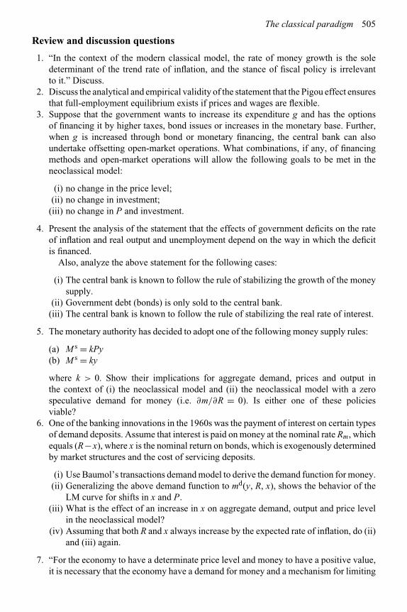
The classical paradigm 505
Review and discussion questions
1. “In the context of the modern classical model, the rate of money growth is the soledeterminant of the trend rate of inflation, and the stance of fiscal policy is irrelevantto it.” Discuss.
2. Discuss the analytical and empirical validity of the statement that the Pigou effect ensuresthat full-employment equilibrium exists if prices and wages are flexible.
3. Suppose that the government wants to increase its expenditure g and has the optionsof financing it by higher taxes, bond issues or increases in the monetary base. Further,when g is increased through bond or monetary financing, the central bank can alsoundertake offsetting open-market operations. What combinations, if any, of financingmethods and open-market operations will allow the following goals to be met in theneoclassical model:
(i) no change in the price level;(ii) no change in investment;(iii) no change in P and investment.
4. Present the analysis of the statement that the effects of government deficits on the rateof inflation and real output and unemployment depend on the way in which the deficitis financed.
Also, analyze the above statement for the following cases:
(i) The central bank is known to follow the rule of stabilizing the growth of the moneysupply.
(ii) Government debt (bonds) is only sold to the central bank.(iii) The central bank is known to follow the rule of stabilizing the real rate of interest.
5. The monetary authority has decided to adopt one of the following money supply rules:
(a) M s = kPy(b) M s = ky
where k > 0. Show their implications for aggregate demand, prices and output inthe context of (i) the neoclassical model and (ii) the neoclassical model with a zerospeculative demand for money (i.e. ∂m/∂R = 0). Is either one of these policiesviable?
6. One of the banking innovations in the 1960s was the payment of interest on certain typesof demand deposits. Assume that interest is paid on money at the nominal rate Rm, whichequals (R−x), where x is the nominal return on bonds, which is exogenously determinedby market structures and the cost of servicing deposits.
(i) Use Baumol’s transactions demand model to derive the demand function for money.(ii) Generalizing the above demand function to md(y, R, x), shows the behavior of the
LM curve for shifts in x and P.(iii) What is the effect of an increase in x on aggregate demand, output and price level
in the neoclassical model?(iv) Assuming that both R and x always increase by the expected rate of inflation, do (ii)
and (iii) again.
7. “For the economy to have a determinate price level and money to have a positive value,it is necessary that the economy have a demand for money and a mechanism for limiting
506 Monetary policy and the macroeconomy
its supply.” Discuss in the context of (a) the quantity theory, (b) neoclassical economicswith an exogenous money supply, and (c) privately issued monies.
8. “In a closed economy, if the money stock is held constant by the central bank, an increasein the government deficit does not have either short-run or long-run effects on aggregatedemand and output.” Discuss in the context of the neoclassical model and the newclassical model (with rational expectations and Ricardian equivalence).
9. Discuss whether the existence of business cycles and the observed positive correlationbetween real and monetary variables mean that the modern classical models are neithervalid nor relevant for policy purposes.
10. Specify a model that generates real business cycles only. Discuss whether this modelallows for the observed cyclical correlation between money and output.
11. Present the new classical model (with rational expectations and Ricardian equivalence).Analyze the role of monetary policy in this model.
How would this model explain the major recession in the early 1990s in most developedeconomies? What monetary policies – if any – are consistent with this model formoderating the effects of the recession on output and unemployment?
12. Discuss the proposition that a change in the rate of growth of the money supply will notaffect output and unemployment in the short run, as well as in the long run, if wages andprices are fully flexible.
13. “The rate of money growth is the sole determinant of aggregate demand and the trendrate of inflation, and the stance of fiscal policy is irrelevant.” Discuss.
14. “In response to demand shocks, short-term price adjustments by markets occur earlierthan quantity adjustments at the level of both the firm and the economy.” Discussthe relevant theory behind this statement. Also, discuss its empirical validity at themacroeconomic level.
15. The “crowding out” hypothesis asserts that investment is crowded out by fiscal deficits.Is it fully or partially valid in (i) the IS–LM model, (ii) the neoclassical model, or (iii) thelong-run equilibrium of the modern classical approach? As part of your answer, discuss:can complete crowding out occur in the context of (a) a financially advanced economy,(b) a financially under-developed economy?
16. The 1970s monetarism and the new classical school are sometimes lumped under thesame banner. How do these schools view the existence of short-run unemployment inthe economy and what policies does each imply for curing it? What role do the schoolsassign to monetary policy in this respect?
17. What are main tenets of the modern classical school and how do they differ from thoseof the traditional classical school?
Discuss critically the contributions of the modern classical school to our understandingof the role and limitations of monetary and fiscal policies for stabilization, and comparethese with those of the neoclassical model.
18. Discuss the empirical validity of the implications of the modern classical model for(i) the long run, (ii) the short run.
19. What is the empirical assessment by Lucas of the importance of short-run fluctuations inunemployment and output due to errors in expectations? Discuss other possible reasonsfor such fluctuations.
20. How do (i) real business cycle theory, (ii) Friedman–Lucas supply analysis, explain fluc-tuations in unemployment over the business cycle? What is the impact on unemploymentof changes in aggregate demand in these models? How would you test the validity ofthe implications of these theories?

The classical paradigm 507
21. If the central bank cannot change output and unemployment through systematic moneysupply changes and its induced changes in the anticipated inflation rate, should it tryto do so by changes in the unanticipated inflation rate? If such unanticipated inflationrequires a random change in the money supply, how can the central bank achieve this?What will be the effect of such a random change on output and unemployment, and whatconclusions can be drawn on the advisability of such a monetary policy? Discuss.
References
Andersen, L.C., and Jordan, J.L. “Monetary and fiscal actions: a test of their relative importance ineconomic stabilization.” Federal Reserve Bank of St. Louis Review, 50, 1968, pp. 11–24.
Ball, L. “How credible is disinflation? The historical evidence.” Federal Reserve Bank of PhiladelphiaBusiness Review, 1993, pp. 17–28.
Barro, R.J. “Are government bonds net wealth?’ Journal of Political Economy, 82, 1974, pp. 1095–118.Barro, R.J. “Unanticipated money growth and unemployment in the United States.” American Economic
Review, 67, 1977, pp. 101–15.Barro, R.J. “Inflation and growth.” Federal Reserve Bank of St. Louis Review 78, 1996, pp. 153–69.Brayton, F., and Tinsley, P. “A guide to FRB/US: a macroeconomic model of the United States.”
Federal Reserve Board Finance and Economic Discussion Series, 1996–42, 1996.Bullard, J., and Keating, J.W. “The long-run relationship between inflation and output in postwar
economies.” Journal of Monetary Economics, 36, 1995, pp. 477–96.Christiano, L.J., and Eichenbaum, M. “Current real-business-cycle theories and aggregate labour-
market fluctuations.” American Economic Review, 82, 1992, pp. 430–50.Christiano, L.J., Eichenbaum, M., and Evans, C. “Monetary policy shocks: What have we learned and to
what end.” In J. Taylor and M. Woodford eds, Handbook of Macroeconomics, vol. 1A. Amsterdam:Elsevier North-Holland, 1999, pp. 65–148.
Cover, J.P. “Asymmetric effects of positive and negative money supply shocks.” Quarterly Journal ofEconomics, 107, 1992, pp. 1261–82.
Eichenbaum, M. “Comments: interpreting the macroeconomic time series facts: the effects of monetarypolicy.” European Economic Review, 36, 1992, pp. 1001–11.
Friedman, B.M. “The LM curve: a not-so-fond farewell.” NBER Working Paper no. 10123, 2003.Friedman, M. “The supply of money and changes in prices and output” (1958). Reprinted in M. Friedman
The Optimum Quantity of Money and Other Essays. Chicago: Aldine, 1969, pp. 171–87.Friedman, M. A Program for Monetary Stability. New York: Fordham University Press, 1959.Friedman, M. “The role of monetary policy.” American Economic Review, 58, 1968, pp. 1–17.
Reprinted in Milton Friedman, The Optimum Quantity of Money and Other Essays. Chicago: Aldine,1969, pp. 95–110.
Friedman, M. “A theoretical framework for monetary analysis.” Journal of Political Economy, 78,1970, pp. 193–238.
Friedman, M. “Nobel prize lecture: inflation and unemployment.” Journal of Political Economy, 85,1977, pp. 451–73.
Friedman, M., and Schwartz, A. “A monetary history of the United States, 1867–1960.” Chicago:University of Chicago Press, 1963a.
Friedman, M., and Schwartz, A. “Money and business cycle.” Review of Economics and Statistics, 45,1963b, pp. 32–64.
Geweke, J. “The superneutrality of money in the United States: an interpretation of the evidence.”Econometrica, 54, 1986, pp. 1–22.
Hicks, J.R. “Mr. Keynes and the classics: a suggested interpretation.” Econometrica, 5, 1937,pp. 147–59.
Hume, D. Of Money (1752). Reprinted in The Philosophical Works Of David Hume, 4 volumes. Boston:Little, Brown, 1954.

508 Monetary policy and the macroeconomy
Ireland, P.N. “Money’s role in the monetary business cycle.” NBER Working Paper no. 8115,2001a.
Ireland, P.N. “Sticky-price models of the business cycle: specification and stability.” Journal ofMonetary Economics, 47, 2001b, pp. 3–18.
Keynes, J.M. The General Theory of Employment, Interest and Money. New York: Macmillan, 1936.Kormendi, R.C., and Meguire, P.G. “Cross-regime evidence of macroeconomic rationality.” Journal
of Political Economy, 92, 1984, pp. 875–908.Lucas, R.E., Jr. “Expectations and the neutrality of money.” Journal of Economic Theory, 4, 1972,
pp. 103–24.Lucas, R.E., Jr. “Some international evidence on output–inflation tradeoffs.” American Economic
Review, 63, 1973, pp. 326–34.Lucas, R.E., Jr. “Comments on Ball and Mankiw.” Carnegie-Rochester Series on Public Policy, 41,
1994, pp. 153–5.Lucas, R.E., Jr. “Nobel lecture: monetary neutrality.” Journal of Political Economy, 104, 1996,
pp. 661–82.McCandless, G.T., Jr., and Weber, W.E. “Some monetary facts.” Federal Reserve Bank of Minneapolis
Quarterly Review, 19, 1995, pp. 2–11.Mankiw, N.G. “The inexorable and mysterious tradeoff between inflation and unemployment.”
Economic Journal, 111, 2001, pp. C45–61.Mishkin, F.S. “Does anticipated aggregate demand policy matter?” American Economic Review, 72,
1982, pp. 788–802.Mishkin, F.S. “Is the Fisher effect for real? A reexamination of the relationship between inflation and
interest rates.” Journal of Monetary Economics, 30, 1992, pp. 195–215.Monnet, C., and Weber, W. “Money and interest rates.” Federal Reserve Bank of Minneapolis Quarterly
Review, 25, 2001, pp. 2–13.Mosser, P. “Changes in monetary policy effectiveness: evidence from large macroeconomic models.”
Federal Reserve Board of New York Quarterly Review, 17, 1992, pp. 36–51.Nelson E. “Sluggish inflation and optimising models of the business cycle.” Journal of Monetary
Economics, 42, 1998, pp. 302–22.Parkin, M. “Essays on and in the Chicago tradition.” Journal of Money, Credit and Banking, 18, 1986,
pp. 104–21.Patinkin, D. Money, Interest and Prices. 2nd edn. New York: Harper & Row, 1965.Patinkin, D. “The Chicago tradition, the quantity theory, and Friedman.” Journal of Money, Credit and
Banking, 1, 1969, pp. 46–70.Patinkin, D. “Friedman on the quantity theory and Keynesian economics.” Journal of Political Economy,
80, 1972, pp. 883–905.Pesek, B.P. Microeconomics of Money and Banking and Other Essays. New York: Harvester
Wheatsheaf, 1988.Phelps, E.S. “Money-wage dynamics and labor market equilibrium.” Journal of Political Economy,
76, 1968, pp. 678–711.Pigou, A.C. “Money, a veil?” In The Veil of money. London: Macmillan, 1941, Ch. 4.Prescott, E.C. “Theory ahead of business cycle measurement.” Carnegie-Rochester Conference Series
on Public Policy, 25, 1986, pp. 11–44.Romer, D. Advanced Macroeconomics. New York: McGraw-Hill, 1996.Sargent, T.J., and Wallace, N. “Rational expectations, the optimal monetary instrument, and the optimal
money supply rule.” Journal of Political Economy, 83, 1975, pp. 241–54.Sargent, T.J., and Wallace, N. “Rational expectations and the theory of economic policy.” Journal of
Monetary Economics, 2, 1976, pp. 169–83.Sims, C.A. “Money, income and causality.” American Economic Review, 62, 1972, pp. 540–2.Sims, C.A. “Interpreting the time series facts: the effects of monetary policy.” European Economic
Review, 36, 1992, pp. 975–1000.
The classical paradigm 509
Taylor, J.B. “How should monetary policy respond to shocks while maintaining long-run pricestability? – Conceptual issues.” In Achieving Price Stability, Federal Reserve Bank of Kansas City,1996, pp. 181–95.
Walsh, C.E. Monetary Theory and Policy. 2nd edn. Cambridge, MA: MIT Press, 2003.Wong, K. “Variability in the effects of monetary policy on economic policy.” Journal of Money, Credit,
and Banking, 32, 2000, pp. 179–98.
15 The Keynesian paradigm
The Keynesian tradition differs from the classical one in not assuming that the economy isalways in equilibrium with full employment or, if out of equilibrium, tends on its own tofull employment within a reasonably short time. This was the core assertion of Keynes’sThe General Theory, published in 1936, and remains at the core of all models withinthe Keynesian tradition. This assertion has the corollary that appropriate macroeconomicpolicies could improve on the functioning of the economy. Most central banks do follow thisrecommendation.
The Keynesian model has been evolving ever since its basis was laid in Keynes’scontributions in 1936. It has gone through many versions, with different versions taking centrestage at different stages in its evolution and many coexisting simultaneously. Its latest versionis the new Keynesian model.
Key concepts introduced in this chapter
♦ Involuntary unemployment♦ Phillips curve♦ Demand-deficient Keynesian model♦ NeoKeynesian model♦ New Keynesian model♦ Notional demand and supply functions♦ Effective demand and supply functions♦ Sticky prices♦ Staggered wage contracts♦ Implicit employment contracts♦ Efficiency wages♦ Taylor rule♦ New Keynesian Phillips curve
This chapter reviews the Keynesian ideas on short-run macroeconomics. To start, the materialon the Keynesian paradigm in Chapter 1 should be reviewed. That presentation argued thatthe Keynesian paradigm was the study of the pathology of the macroeconomy: it focuses onthe causes, implications and policy prescriptions for the deviations of the economy from itsWalrasian general equilibrium position and holds that the pursuit of appropriate monetaryand fiscal policies can shorten the extent and/or duration of the deviation. Since there can be

The Keynesian paradigm 511
many causes of such deviations, their appropriate study requires not one unified model butmany, some of which will be variations on the same theme, but there could also be modelsthat are incompatible with one another. As such, there is no one model that can lay claim tobe the Keynesian model. This chapter provides a small sample of the diversity of Keynesianmodels.
Since the classical model implies only transitory and self-correcting deviations fromfull employment, its emphasis tends to be on finding the long-run relationships. Sincethe Keynesian paradigm holds that deviations from full employment may not always betransitory and self-correcting, its focus is on finding the short-run dynamic relationships andthe policies appropriate to them.1 Keynes himself had expressed his strong disapproval ofthe long-run focus of classical macroeconomics in his time (and continuing at the presenttime) in:
But this long run is a misleading guide to current affairs. In the long run we are all dead.Economists set themselves too easy, too useless a task if in tempestuous seasons theycan only tell us that when the storm is long past the ocean is flat again.
(Keynes, 1923, p. 80).
Keynesianism is a living tradition, evolving and refining its ideas over time, so that thereare several versions of the Keynesian approach. The original version was Keynes’s own ideasas set out in The General Theory (1936), followed by a number of evolving and quite diverseversions of the Keynesian framework,2 representing a broad and often somewhat disparateset of ideas. While some of the earlier versions of Keynesianism are still part of its currentmainstream, its most recent version is the new Keynesian (NK) one, which emerged onlyin the 1990s. Given this diversity, one needs to focus on the core themes in the Keynesianparadigm as a whole.
The common strands in the Keynesian approaches, broadly defined, are the reliance onsome form of market imperfections and the angst over the performance of the economy,especially of the labor and commodity markets. Additional themes in the Keynesianliterature, as in Keynes’s The General Theory, are: the impact of changes in aggregatedemand on output and employment, animal spirits (economic agents’ psychology) anddegree of confidence, market psychology, a consumption function that bases actualconsumption on actual income through the multiplier, liquidity preference, presence ofuncertainty and the possibility of default in financial markets (so that not all bondscan be assumed to be one-period riskless ones), moral hazard and contagion in finan-cial markets, and macroeconomic instability rather than stability. While we touch onsome of these topics at various places in this book, most are left to more specializedstudies.
Keynesian models reject the perfectly competitive functioning of the labor market.Over time, given the complexity of this market, different Keynesian models have resorted
1 Therefore, in empirical analysis using cointegration and error-correction techniques, the concern of the classicalanalysis is mainly with the properties of the cointegrating vector, while that of the Keynesian paradigm is mainlywith the coefficients of the error-correction equation.
2 There is considerable dispute as to whether any of the Keynesian models represents Keynes’s own work. A closereading of Chapters 2 and 3 of The General Theory shows that they do not. It is therefore appropriate tomake a distinction between the Keynesian models and Keynes’s own analysis, though the former arose outof interpretations of the latter.

512 Monetary policy and the macroeconomy
to different simplifying assumptions about it. At the risk of oversimplification, thesewere that:
(i) The nominal wage is fixed (1940s and early 1950s).(ii) The nominal wage is variable but the supply of labor depends on the nominal and not
the real wage (1950s and 1960s).(iii) The structure of the labor market can be replaced by the Phillips curve (late 1950s and
early 1960s) or the expectations-augmented Phillips curve (late 1960s).(vi) The demand and supply of labor depend on the expected real (not nominal) wage, but
the expectations on prices, needed to derive the expected real wage from the negotiatednominal wage, are subject to errors and asymmetric information between firms andworkers (1970s and 1980s). Wage contracts are in nominal terms and staggered overtime.
(v) The focus of the Keynesian analysis is on states other than full employment, so thatthe notional demand and supply functions of Walrasian and neoclassical economics arenot applicable. The applicable concepts are those of effective demand and supply andthe equilibrium – or “temporary equilibrium” as it is called by some writers – betweenthem can occur at less than full employment and have different dynamic propertiesfrom those of neoclassical economics or its disequilibrium analysis. Such analysis issometimes presented in the form of quantity-constrained models (1970s and 1980s).
(vi) In the labor market, the real wage is an efficiency real wage that can be rigid in theshort run. In addition, commodity prices are sticky. Labor markets also have implicitcontracts and firm-specific skills. In the commodity market, prices are sticky becauseof menu costs (1980s and 1990s).
(vii) The economy has forward-looking, monopolistically competitive firms that optimizeintertemporally, yielding staggered, discrete adjustment of individual commodityprices. In the aggregate, this results in an NK Phillips curve relationship with theprice level adjusting more slowly than in a Walrasian economy with money neutrality.Further, on monetary policy, the forward-looking optimizing central bank follows aTaylor rule for setting its interest rate (after about the mid-1990s).
The intention of this chapter is not to go through each of the various versions of theKeynesian approach but to present just three versions to show the general pattern and varietyof their reasoning and implications for monetary and fiscal policies. The common themeamong these versions of the Keynesian ideas is that money is not neutral in the short runand that aggregate demand management can help to improve on its performance. The modelsthat will be used to show this are the disequilibrium or temporary equilibrium (also calledthe demand-deficient) model, the Phillips curve model and the NK model. Our presentationwill cover the following models and ideas:
(I) The demand and supply functions are as in the neoclassical model but the labor marketdoes not always clear, or clear fast enough, in notional terms. Further, economic agentsreact faster than markets to disequilibrium once it has emerged. The models used for thispresentation are the effective (deficient) demand ones with involuntary unemployment.
(II) The individual equations of the labor market are replaced by the Phillips curve as amode of encapsulating the behavior of the labor market and variations in it.
(III) There are various aspects, such as staggered nominal wage contracts, implicit contracts,efficiency wages, menu costs, etc., that affect the functioning of the labor and

The Keynesian paradigm 513
commodity markets. These somewhat disparate ideas, as compared to an integratedmacroeconomic model, can be grouped under the label of NeoKeynesian economics.
(IV) The final model presented is that of the integrated NK approach, encompassing an NKprice adjustment process (the NK Phillips curve) and a Taylor rule to set the economy’sreal interest rate. This approach differs from the preceding ones by using a stochasticintertemporal general equilibrium model with monopolistically competitive firms toderive the price adjustment equations of the macroeconomic model.
Keynesian models omitted from our presentation
In particular, the models that are within the Keynesian tradition but have been omitted fromthis chapter are:
(a) Those that assume that the supply of labor depends in some way on the nominal wageand not merely on the real one. The extreme form of this hypothesis, that the nominalwage is rigid downwards, is also not presented. The latter was popular in the 1940sand 1950s and the former was common in the 1960s. Neither is now in vogue amongKeynesian economists.
(b) The labor market clears but the supply of labor depends on the expected real wage,and price expectations are subject to imperfect and asymmetric information. Since sucha model involves uncertainty and expectations, its presentation is to be found in thepreceding chapter’s analysis of the expectations-augmented Phillips curve (EAPC).
(c) Many Keynesians in the 1950s and the 1960s argued that inflation was due to themarket power of monopolistic firms and/or labor unions. In some of these (cost-push)models, unions pushed for higher wages, firms followed a full-cost pricing policy andthe central bank accommodated the money supply to the price level so as not to raise theunemployment rate.
On the product, money and bond markets, most Keynesians up to the mid-1990s seemedwilling to accept the assumption that the central bank exogenously provides the money supplyto the economy, as well as the IS–LM model’s Keynesian–neoclassical synthesis of aggregatedemand, which had evolved by the 1960s. The more recent (post-mid-1990s) new Keynesianmodels discard the LM curve, assuming that the central bank exogenously sets the interestrate or follows a Taylor rule on it, and combine it with an IS equation. The relevant IS–LMand IS–IRT models of aggregate demand in the open economy were presented in Chapter 13.This chapter takes their analysis of aggregate demand as given.
A caution on the categorization of Keynesian models
The following cautionary notes at this stage might provide some general guidance incomparing the neoclassical and Keynesian paradigms.
1 Keynesians in general accept the specification and conclusions of the classical paradigmon the long-run equilibrium of the economy. That is, in long-run equilibrium, theeconomy will have full employment and money neutrality. However, the Keynesianmodels differ from the classical paradigm in their conclusions about the short-run andshort-term functioning of the economy. In particular, they focus on those deviations fromlong-run equilibrium that are not necessarily transient and self-correcting.

514 Monetary policy and the macroeconomy
2 It is often contended that the distinguishing difference between the classical andKeynesian paradigms is that the former assumes the flexibility of nominal wages and/orprices, while the latter assumes them to be rigid. As will be shown in this chapter, therigidity of nominal wages and/or prices is not a necessary component of some of theKeynesian versions. This is not to say that the Keynesian models cannot be based onsuch an assumption; it is rather to assert that they do not necessarily require such anassumption and that the qualitatively distinct Keynesian policy results can be derivedwith flexible prices and nominal wages provided that the condition of instantaneousmarket clearance is not imposed.
3 Further, the Keynesian models do not necessarily need to rely upon irrational (such asprice illusion) or myopic (one-period optimization) economic behavior but can derivetheir distinctive conclusions under the rational demand and supply behavior of economicagents, given the conditions that come about in the relevant markets.
4 It is sometimes contended that while the Keynesian models study disequilibrium inthe economy, classical models study its equilibrium properties. However, while someKeynesian models do focus on disequilibrium, others, such as the NK model, imposethe requirement of general equilibrium, in which all markets are assumed to clear.
5 It is also often contended that, while the (current) models of the classical paradigmare based on micro foundations with optimal behavior by economic agents, those ofthe Keynesian models are not so based. This is not always so. The current crop ofnew Keynesian models derives its macro relationships from micro foundations withoptimizing behavior.
Sections 15.1 to 15.4 present three of the main versions of the Keynesian model.Section 15.5 derives the reduced-form Keynesian relationship between output and the moneysupply. Section 15.6 presents the empirical assessment of the validity of the Keynesian model.
15.1 Keynesian model I: models without efficient labor markets
A market is efficient if it instantly restores equilibrium following any shift in demand orsupply. Conversely, an inefficient market is one that does not have instantaneous marketclearance. In the context of the labor market, note that this market is really very many diversemarkets, separated by skills, location, different firms, and so on, and often with implicitlong-term contracts and insider–outsider trading, etc. These factors provide plenty of scopefor those who want to assume that the labor market is not efficient, while leaving others toassume that it can be taken to be efficient, or approximately so, for macroeconomic analysis.
Keynes (1936) argued that in a monetary economy the worker is generally paid a wagerate that is not guaranteed in terms of its purchasing power but is, rather, a nominal wagerate. It is the nominal wage rate that is negotiated between an employee or his union and theemployer. Once a nominal wage rate has been set in an explicit or implicit contract, undernormal economic circumstances neither the employee nor his union seems willing to accepta cutback in the set wage rate. However, while workers are not willing to accept a cutback innominal wage rates, they seem more willing to tolerate a reduction in the purchasing powerof their nominal wage if this is brought about by changes in the purchasing power of money.3
3 This is, however, a short-term phenomenon in the modern industrialized economy. Workers and their unionsare nowadays sufficiently sophisticated to realize the losses in real income due to inflation and try to base the

The Keynesian paradigm 515
A simple version of this (“rigid wage”) model, in which the nominal wage rates are assumedto be rigid downwards, was an early version (1940s and 1950s) of the Keynesian model. Thiswas supplanted in the 1950s and 1960s by a “nominal wage model” in which the supply oflabor depended on the nominal wage rate, which was flexible and determined by the labormarket.4 However, these two models are not now seriously included among the models ofthe Keynesian paradigm and are omitted from this edition. Those still interested in theirexposition can find the latter in Handa (2000, Ch. 15) or Patinkin (1965, Ch. 13). However,we note in passing that the assumptions of this nominal-wage model did not include therigidity of nominal wages and prices, or of real wages, nor did it imply it. Further, this modelassumed market clearance, but at the equilibrium nominal, not real, wage.
The assumption of labor supply depending on the nominal rather than the real wage impliesmoney illusion or myopia by labor, which is empirically not valid over any extended periodof time. Many Keynesians and especially post-Keynesians have argued that Keynes’s TheGeneral Theory did not make this assumption but agreed with the neoclassical assumptionthat workers would base the supply of labor on the purchasing power of the nominal wage,i.e. on the real wage rate. They also argue that Keynes assumed that the modern economy, withnumerous industries and firms and with decentralized wage negotiations, does not possessa mechanism that would ensure that the labor markets are normally in equilibrium at fullemployment with an equilibrium real wage. Hence, the claim being made under this argumentis that the major distinction between the Keynesian and the neoclassical models is that, whilethe neoclassical model makes the assumption of labor market equilibrium as the usual state,Keynes did not do so. That is, Keynesian models of this type specify the labor market demandand supply functions as:
nd = nd(w) ∂nd/∂w < 0 (1)
ns = ns(w) ∂ns/∂w > 0 (2)
These behavioral functions are identical with those in the neoclassical model. However, onthe basis of the empirical belief that the labor markets are usually not in long-run equilibrium,there is no assumption of labor market equilibrium in this type of Keynesian model. Sincefirms are assumed to be able to hire the amount of labor that they demand, the market clearancecondition (n = nf = nd = ns) of the neoclassical model is replaced by:
n = nd ≤ ns (3)
Note that (3) does not assume that labor market equilibrium at full employment willnever exist in the economy. This equation implicitly assumes that the modern capitalisteconomy does not possess sufficient mechanisms to ensure continuous full-employmentequilibrium or achieve it within a reasonable period of time after a shock. Further, such an
negotiated wage on the expected rate of inflation. If the actual inflation rate is higher than the expected one,workers try to get compensation for it at the next round of wage negotiations, so that in the long run labor supplywill be effectively based on the real wage rather than on nominal wages. We will return to these considerationsat a later stage in this chapter.
4 The above is clearly a rather simplified picture of the wage bargain. A somewhat better picture emerges if it isassumed that workers supply labor on the basis of the expected real wage rate and the expectations are explicitlymodeled. This is particularly so when nominal wage rates and prices are rising and it is difficult for workers toperceive the actual change in the real wage rate.
516 Monetary policy and the macroeconomy
economy can get stuck at a level of employment below full employment, and these levels canalso be equilibrium states.5 That is, the Keynesian models allow the possibility of multiplemacroeconomic equilibria, each with a different level of output and unemployment. Oneof these equilibria is that of full employment, so that we have to distinguish between thefull-employment equilibrium and other equilibria with less than full employment.
The justification for involuntary unemployment
Designate the long-run equilibrium (full-employment) level of employment as nf , and the rateof unemployment consistent with it as un · un is the natural or Walrasian (full-employment)equilibrium rate of unemployment consistent with the structure of the economy, includingany wage rigidities such as specific skills, minimum wage laws, labor unions and workpreferences. Also designate the short-run equilibrium unemployment rate as u∗, which differsfrom un due to errors in price expectations and the costs of adjusting prices, employment,output, etc. Separate the two components of u∗ due to expectations errors, which is anelement of the short-run modern classical model (see Chapter 14), and those due to adjustmentcosts, some of which underlie many Keynesian models (see Section 15.3), as u′∗ and u′′∗,respectively with u∗ = u′∗ + u′′∗.
Note the identity.
u ≡ un + (u∗ − un) + (u − u∗) (4)
If there are no errors in price expectations and no adjustment costs, u∗ (short-run equilibriumunemployment rate) will be identical with un (long-run equilibrium unemployment rate).Since the actual economy cannot be expected to be always and at every instant in equilibrium,or, as Keynes would have claimed, in equilibrium most of the time, (u − u∗) would notalways equal zero. Define ui ≡ u − u∗, where ui is the deviation of unemployment from itsshort-run equilibrium value. With un + (u∗ −un) as the short-run equilibrium unemploymentrate, ui will be indicative of the failure of the economy to be in either short-run or long-runequilibrium. ui is usually labeled the involuntary unemployment rate. Its value can be positive,zero or negative, with a negative value likely to occur near the peak and a positive value nearthe trough of the business cycle. From the perspective of the actual economy and policy,ui would be zero only if the economy, not the model, is operating in equilibrium. From theperspective of a model, ui would be zero in the solution of the model if the analytical conditionof short-run equilibrium is imposed in deriving the solution. Keynes and the Keynesians (otherthan the new Keynesians) used the former perspective and argued that the actual economyis usually not in equilibrium. Further, given their focus on deficient demand rather than onexcess demand, their analysis implied positive involuntary unemployment when demand isdeficient relative to the short-run equilibrium output level.
Keynesians argue, therefore, that the authorities should keep a close watch on the economyand, when there is significant involuntary unemployment due to a deficiency in aggregatedemand, they should use monetary and/or fiscal policies to increase demand by an appropriateamount. If they succeed, the economy will eliminate such involuntary unemployment andperform at its full employment potential.
5 The term “equilibrium” is defined here as a state from which there is no inherent tendency to change. It specifiesthe values of the endogenous variables implied by the model for a specified set of values of the exogenous variablesin the model.

The Keynesian paradigm 517
The class of models that fit the preceding remarks are often called “deficient-demandmodels,” though they allow the absence of deficient demand in the limiting case of fullemployment. The following subsection presents an example of a deficient-demand analysis,noting that there can also be other versions that fall into this category.
15.1.1 Keynesian deficient-demand model: quantity-constrained analysis
Keynes had argued that the economy may not always generate aggregate demand equalto the full-employment supply of commodities. The former comes from the decisions ofvery many households, firms and the government (and exports in the open economy) in theform of consumption, investment and government expenditures. The latter is generated byfirms, which undertake production to meet expected sales. There is no a priori reason forthe two to be equal. The two could, however, be brought into equality by efficient marketsthat adjust the price to the equilibrium level. However, Keynes argued that the marketswere not efficient (i.e. following a shift in demand or supply, adjusting the price instantly toequate demand and supply), so that firms and households would make their production andconsumption decisions in response to expected demand and incomes, rather than to changes inthe market price. In brief, markets were sluggish in their adjustment, and firms and householdsreacted faster than markets. This implies that firms would base their output and investmenton expected demand, so that changes in aggregate demand would change aggregate outputand employment. Households, in deciding on their consumption expenditures, reacted totheir expected income and job prospects and not merely to their real wage rate, so that theirconsumption, and therefore aggregate demand, would respond to their job prospects. Hence,a fall in aggregate demand would reduce output and employment, which would, in turn,worsen incomes and job prospects and lower consumption (Clower, 1965; Patinkin, 1965;Leijonhufvud, 1967, 1968).
Writing in the Great Depression, Keynes argued that the economy often functions belowits full-employment level. While a depression has not been experienced since the 1930sby the major economies, all economies do suffer periodic recessions. Keynes’s factualstatement is generally taken to be correct for recessions.6 The most plausible reason foroutput falling below its full-employment level is a demand deficiency originating witha fall in aggregate demand. To show this, start with the initial state of full-employmentequilibrium in the economy and assume that aggregate demand falls for some reason,thereby creating deficient demand relative to the full-employment level. Following the ideasof the preceding section, assume that the labor market does not instantly clear, so thatsome of the workers become involuntarily unemployed because of the fall in aggregatedemand. These workers will not receive the wage they would have got if they had beenable to sell their labor according to their supply curve. Their lack of income forces themto reduce their demand for commodities and real balances below that specified by theirWalrasian functions as derived in Chapter 3 and the neoclassical functions specified inChapter 14. Hence, these latter functions are not “effective” – that is, operational – in thestate of involuntary unemployment. They can only be effective if there is full employmentin the economy and workers could sell all the labor they wanted to at the existingwage rate.
6 It is a well-established stylized fact that virtually all recessions have a fall in aggregate demand and a fall inoutput, as well as a fall in the inflation rate.
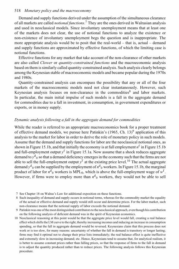
518 Monetary policy and the macroeconomy
Demand and supply functions derived under the assumption of the simultaneous clearanceof all markets are called notional functions.7 They are the ones derived in Walrasian analysisand used in neoclassical models. Since involuntary unemployment means that at least oneof the markets does not clear, the use of notional functions to analyze the existence ornon-existence of involuntary unemployment begs the question and is inappropriate. Themore appropriate analysis would be to posit that the real-world – that is, actual – demandand supply functions are approximated by effective functions, of which the limiting case isnotional functions.
Effective functions for any market that take account of the non-clearance of other marketsare also called Clower or quantity-constrained functions and the macroeconomic analysisbased on them is similarly called quantity-constrained analysis. Such analysis clearly belongsamong the Keynesian stable of macroeconomic models and became popular during the 1970sand 1980s.
Quantity-constrained analysis can encompass the possibility that any or all of the fourmarkets of the macroeconomic models need not clear instantaneously. However, suchKeynesian analysis focuses on non-clearance in the commodities8 and labor markets.In particular, the main initial impulse of such models is a fall in the aggregate demandfor commodities due to a fall in investment, in consumption, in government expenditures orexports, or in money supply.
Dynamic analysis following a fall in the aggregate demand for commodities
While the reader is referred to an appropriate macroeconomics book for a proper treatmentof effective demand models, we pursue here Patinkin’s (1965, Ch. 13)9 application of thisanalysis to the market for labor in order to derive the role of monetary policy in such models.Assume that the demand and supply functions for labor are the neoclassical notional ones, asshown in Figure 15.1b, and that initially the economy is at full employment nf in Figure 15.1band full-employment output yf in Figure 15.1a. Now assume that a shock reduces aggregatedemand to yd
0 so that a demand deficiency emerges in the economy such that the firms are notable to sell the full-employment output yf at the existing price level.10 The actual aggregatedemand yd
0 can be supplied by the employment of nd0 workers. In Figure 15.1b, the marginal
product of labor for nd0 workers is MPL0, which is above the full-employment wage of wf .
However, if firms were to employ more than nd0 workers, they would not be able to sell
7 See Chapter 18 on Walras’s Law for additional exposition on these functions.8 Such inequality of demand and supply occurs in notional terms, whereas for the commodity market the equality
of the actual or effective demand and supply would still occur and determine prices. For the labor market, suchnon-clearance means that the notional supply of labor exceeds the notional demand.
9 Patinkin was one of the most distinguished contributors to the neoclassical approach, even though his contributionon the following analysis of deficient demand was in the spirit of Keynesian economics.
10 Neoclassical reasoning at this point would be that the aggregate price level would fall, creating a real balanceeffect which shifts the LM curve to the right, thereby increasing incomes and inducing an increase in consumptionspending, so that the fall in aggregate demand would be reversed. Keynesians claim that this process does notwork or is too slow, for many reasons: uncertainty of whether the fall in demand is transitory or longer lasting;firms may find it optimal not to change their price lists immediately; the real balance effect is quite ineffectiveand extremely slow in increasing demand; etc. Hence, Keynesians tend to assume that, for analytical realism, itis better to assume constant prices rather than falling prices, so that the response of firms to the fall in demandis to adjust the quantity produced rather than to reduce prices. The following analysis follows this Keynesianprocedure.
The Keynesian paradigm 519
nd0 n f
n
y
(a) (b)
y f
yd0
y
nd0 n f
n
w
MPL0=w ′0w f
w ″0
nd′ nd
ns
Figure 15.1
the extra output so that their marginal revenue product would be zero. Hence, if aggregatedemand fell to yd
0, firms would cut employment to only nd0 workers.11
Extending this argument to Figure 15.1b, the employed nd0 workers can be paid nominal
wage rates which can change, as can the price level, with the resultant real wage beinganywhere within the range w′
0 and w′′0, without a change in the firms’ employment of nd
0
workers, so that real wage rates could drift up or down from the initial equilibrium levelof wf .12 Hence, the decrease in employment (from nf to nd
0) can be accompanied by eitheran increase or a decrease in the real wage rate of the employed workers. Wages may thereforefollow a pro-cyclical or counter-cyclical pattern: some recessions and some parts of a givenrecession could show wages falling while others show them to be rising. If wages rise, itcould be claimed that the rise in wages is the cause of falling employment, when this rise isitself only an effect while the true cause was the initial fall in aggregate demand.
The above effects are only partial or initial ones. Since the unemployed workers do notreceive any income, they cut back on their consumption demand. Further, if wages were cutbelow wf , the lower incomes of the employed would also lead to a reduction in consumption.13
The consequent fall in aggregate demand further reduces the effective demand for labor14
and acerbates the recessionary effects derived in the preceding paragraph.The essential components of the preceding analysis are:
(a) The economy’s industrial and market structures do not lead to instant market clearancein all markets, so that rational firms cannot assume this to be so, and must react in their
11 As against this dynamic reaction, neoclassical economics claims that firms will cut prices, not output, in responseto a fall in aggregate demand; or that markets will act fast enough to deliver the lower prices for all commoditiessufficiently to allow firms to sell all they want before individual firms react by cutting their production. Intuitiveknowledge of the economy tends to favor the Keynesian response pattern.
12 Real wages will rise if the price level falls faster than nominal wages, they will fall if the price level falls moreslowly than nominal wages, and will stay constant if both prices and wages fall in the same proportion.
13 The fall in employment usually increases, among the employed workers, the subjective risk of staying employed,so that such workers also tend to cut back on consumption in order to increase precautionary saving to providefor the eventuality of becoming unemployed.
14 The new demand curve is not the neoclassical notional one nd but an effective one, and one cannot proceed withanalysis using nd.
520 Monetary policy and the macroeconomy
production and labor demand strategy to emerging demand conditions for their productsas they see fit. They react faster than markets to changes in demand for products andlabor.
(b) There is no coordinating mechanism or coordinating agency (such as the Walrasianauctioneer with costless and open recontracting while adjustments to a new equilibriumare going on) in the economy which will work out the equilibrium wages, employment,output and prices instantly following shifts in demand and supply. Markets arecompetitive and tâtonnement towards equilibrium values may occur, but takes time,during which firms and workers make decisions on employment.
(c) There is no nominal wage or price rigidity. Prices and wages would be market determinedif the markets were efficient or at least adjusted faster than economic agents in responseto shocks.
(d) Firms and households are rational and react to the conditions that they face in the absenceof perfect markets.
The lack of perfect market structures ensuring instantaneous adjustment to equilibriumor the lack of a coordinating mechanism or agency – with firms and workers not waitingout this process but responding faster than the sluggish markets to a fall in demand is thecritical reason in effective demand models why an economy in which a demand deficiencyhas emerged need not rapidly move to the full-employment level. Critical to the dynamicresponses of economic agents are their rationally expected values (of aggregate demand,prices and employment) that apply in the period (day, month, quarter, etc.) ahead. Theirestimates of these expectations are reflected in some way by economic/business analysts’indices of business and consumer confidence.
It seems reasonable to posit that a very mild fall in aggregate demand in an overall timepath of full employment can leave both business and consumer confidence intact and notproduce a reduction in output and employment, whereas a more significant one or/and over alonger period, especially when backed by past experienced recessions, would produce a lossin such confidence and take the economy onto a dynamic path to involuntary unemploymentlevels. The irony of this remark is that the deliberate pursuit of aggressive Keynesian policiesto maintain aggregate demand at the full-employment level leads to a dynamic response byconsumers and firms which maintains full employment; but a policy of leaving the economyalone, as the classical economists recommend, brings into play dynamic responses whichtake the economy away from full employment. In support of this contention, the Westerneconomies experienced very shallow and short recessions during the Keynesian period ofthe 1950s and 1960s, whereas the recessions lengthened and worsened with the resurgenceof classical economics in the 1980s and 1990s.
Note that new Keynesian models of the post-1990 variety replace the assumption thateconomic agents react faster than sluggish markets by the assumption that firms are pricesetters because they are in monopolistic competition.
Optimal monetary policy in the Keynesian demand-deficient economy
To derive the optimal role and impact of monetary and fiscal policies in such a context,assume that the economy is now at nd
0 of employment and yd0 of output in Figures 15.1a and
15.1b, and suppose the monetary authorities pursue an expansionary monetary policy. Thisincreases aggregate demand in the economy, thereby shifting the nd curve from nd′
towardsnf and increasing output beyond yd
0. Since output increases in response to the increase in

The Keynesian paradigm 521
aggregate demand, prices may or may not increase. The increase in prices will depend onhow deficient the earlier demand was and how large was the earlier excess capacity in theeconomy, but, in any case, prices will not rise in proportion to the increase in the moneysupply.15 The expansionary monetary policy would have succeeded in increasing output inthe economy. But once the economy has reached yf – that is, there no longer exists any demanddeficiency further expansions in the money supply will not increase output but merely causea proportionate increase in the price level. This limiting case of demand-deficient analysis is,of course, the neoclassical full-employment case, in accord with the Keynesians’ claim thattheir analysis is the more general one and encompasses the neoclassical full-employment andclassical cases as a limiting case.
These arguments imply that there is no straightforward or linear relationship betweenincreases in the money supply and real output, or between the rate of inflation and the levelof unemployment. These relationships depend upon the state of the economy and the extentof the monetary expansion. Further, the transmission of the impact of money supply increaseson output does not always require or go through price level increases.
The economy’s responses to excess demand
We have so far considered the dynamics of a decline in demand from a full-employmentlevel. But suppose aggregate demand increases when there already exists full employmentand the economy starts with the natural rate of employment. The dynamic response patternsof firms and workers should be basically consistent, though in opposite directions, in thetwo situations since these would be based on their rational response behavior patterns, butthe economy’s constraints would be quite different between these cases. On the former,the individual firm, seeing an increase in the demand for its product, would tend to increaseproduction through increases in employment, overtime worked, increased effort of employeesand increases in efficiency. Each of these is feasible in the short run, with the increase inemployment, beyond an initial full-employment level, occurring through increased workinghours of part-time workers, through students delaying resumption of studies and throughincreases in the overtime put in by employed workers, etc.16 While such increases inemployment and output above their full-employment levels can and do occur, as long drawn-out booms indicate, their scope is constrained by the economy’s short-run flexibility forthese variables. Hence, while the increases in aggregate demand can and do increase outputand employment in the short run beyond their full employment levels – and the economycan go below its natural rate of unemployment – the increase in prices is more likely, andfaster, than the fall in prices in response to a decline in demand from the full-employmentlevel.
Most central banks now believe that changes in aggregate demand do produce changes inthe economy’s output and that the economy sometimes operates below full employment andsometimes above it. Evidence of these is provided by the current popularity of the Taylorrule, which tries to limit the gap between actual output and full-employment output, as wellas the deviation of inflation from a target level, by the impact of monetary policy on aggregatedemand.
15 The real wage may rise or fall, depending upon where it was earlier in relation to wf .16 However, they cannot be sustained over time (e.g. workers get tired of putting in undesired overtime) and such
increases in employment cannot be assumed for the long run.
522 Monetary policy and the macroeconomy
The eclipse of the deficient-demand analysis
The above deficient-demand analysis was bypassed by new developments, especially thenew Keynesian modeling, in the Keynesian paradigm during the last quarter of the twentiethcentury. One reason for this was that its theoretical development had reached a dead end.Further, it was not intellectually challenging in the context of precise mathematical modeling,especially of macroeconomic dynamics, which had come to dominate macroeconomics.An additional reason was the adoption by the new Keynesians of the intertemporal generalequilibrium methodology under imperfect competition, which, by the nature of its assumptionof general equilibrium, excluded the dynamic effects of deficient demand. However, thisintellectual shunting aside of deficient-demand analysis does not necessarily affect its validity,so that it remains a component analysis of the Keynesian paradigm.
15.2 Keynesian model II: Phillips curve analysis
Phillips curve
In 1958, A.W. Phillips, on the basis of statistical observations for the UK proposed a negativerelationship between the rate of nominal wage growth and the rate of unemployment. Thiswas subsequently extended to show a negative relationship between the rate of inflation andthe rate of unemployment, with the name “Phillips curve” being attached to both of theserelationships. During the late 1950s and the 1960s, Keynesian economics came to embracethis curve, incorporating it in preference to a structural specification of the labor market, asin equations (1) to (3).
Phillips (1958) had plotted the rate of change of nominal wages against the rate ofunemployment for the UK over several periods from 1861 to 1957, and found that the datashowed a downward-sloping curve. That is, the plotted relationship was of the form:
◦W = f (u) (5)
where◦
W is the rate of increase of the nominal wage rate and f ′ < 0. One explanation for (5)is that unemployment represents the degree of labor market tightness, so that the higher thelevel of unemployment, the smaller will be the increase in the nominal wage.
Equation (5) soon evolved into its inverse and then into a relationship of the form:
u = g(π ) (6)
where g′ < 0. This relationship is drawn as the PC curve in Figures 15.2a and 15.2b.The transition from (5) to (6) comes from the link between the nominal wage rate and
inflation: nominal wages represent the main element of the cost of production, so that anincrease in nominal wages will induce firms to increase their prices; alternatively, an increasein prices causes labor to ask for compensation in the form of wage increases. Hence, there isa positive relationship between
◦W and π , which, when substituted into (5), yields (6).
The estimated forms of the Phillips curves proved to be convex to the origin. To explainthis curvature, it was argued that the response of nominal wages to excess demand wasnon-linear, and that decreases in unemployment caused successively greater increases innominal wages. Further, a decrease in employment induces a smaller decline in wages than theincrease in wages brought out by a corresponding increase in job vacancies, so that increases
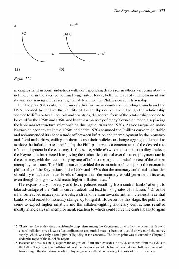
The Keynesian paradigm 523
PC
u
p
(a)
EAPC
u − un
p − p e
(b)
Figure 15.2
in employment in some industries with corresponding decreases in others will bring about anet increase in the average nominal wage rate. Hence, both the level of unemployment andits variance among industries together determined the Phillips curve relationship.
For the pre-1970s data, numerous studies for many countries, including Canada and theUSA, seemed to confirm the validity of the Phillips curve. Even though the relationshipseemed to differ between periods and countries, the general form of the relationship seemed tobe valid for the 1950s and 1960s and became a mainstay of many Keynesian models, replacingthe labor market structural relationships, during the 1960s and 1970s. As a consequence, manyKeynesian economists in the 1960s and early 1970s assumed the Phillips curve to be stableand recommended its use as a trade off between inflation and unemployment by the monetaryand fiscal authorities, calling on them to use their policies to change aggregate demand toachieve the inflation rate specified by the Phillips curve as a concomitant of the desired rateof unemployment in the economy. In this sense, while (6) was a constraint on policy choices,the Keynesians interpreted it as giving the authorities control over the unemployment rate inthe economy, with the accompanying rate of inflation being an undesirable cost of the chosenunemployment rate. The Phillips curve provided the economic tool to support the economicphilosophy of the Keynesians in the 1960s and 1970s that the monetary and fiscal authoritiesshould try to achieve better levels of output than the economy would generate on its own,even though doing so would mean higher inflation rates.17
The expansionary monetary and fiscal policies resulting from central banks’ attempt totake advantage of the Phillips curve tradeoff did lead to rising rates of inflation.18 Once theinflation reached unacceptable levels, with a momentum towards further increases, the centralbanks would resort to monetary stringency to fight it. However, by this stage, the public hadcome to expect higher inflation and the inflation-fighting monetary contractions resultedmostly in increases in unemployment, reaction to which could force the central bank to again
17 There was also at that time considerable skepticism among the Keynesians on whether the central bank couldcontrol inflation, since it was often attributed to cost-push forces, or because it could only control the moneysupply, which was only a small part of liquidity in the economy. The latter point was discussed in Chapter 2under the topic of the Radcliffe report.
18 Boschen and Weise (2003) explore the origins of 73 inflation episodes in OECD countries from the 1960s tothe 1980s. They report that inflation often started because, out of a belief in the short-run Phillips curve, centralbanks sought the short-term benefits of higher growth without considering the costs of disinflation later.
524 Monetary policy and the macroeconomy
pursue a monetary expansion, thereby producing a “stop–go” policy pattern. The role ofexpectations proved vital to the impact of changes in inflation on output and unemployment,and led to the modification of the Phillips curve to the expectations-augmented curve.
The expectations-augmented Phillips curve19
The Phillips curve was challenged by Milton Friedman and the monetarists in the 1960sand 1970s. They argued that if inflation were perfectly anticipated, the labor contractswould reflect it so that the nominal wage would increase by the expected rate of inflation.Consequently, the expected inflation rate would not affect the real wage rate, employmentor output. Hence, at the expected inflation rate, the unemployment rate would be the naturalrate so that only the unanticipated rate of inflation would cause deviations in the actual fromthe natural rate by reducing the real cost of labor and other inputs. That is, according toFriedman, the proper relationship between u and π is not (6) but has the form:
(u∗ − un) = f (π −πe) (7)
with f ′ < 0 and f (0) = 0. un is the long-run equilibrium unemployment rate, while u∗is the short-run equilibrium unemployment rate in the presence of errors in inflationaryexpectations. In the limiting case of expectational equilibrium, an aspect of the “long run,”π = πe and u∗ = un. (7) is the expectations-augmented Phillips curve, as shown as the curveEAPC in Figure 15.2b. Its analysis and policy implications were presented in Chapter 14.
Empirical research and the widespread experience of stagflation in the mid and late 1970s inthe industrialized economies seemed to show that (6) was unstable in a period of acceleratinginflation. Further, (7) seemed to perform much better in such periods, especially at high andaccelerating rates of inflation. In response to this analysis and evidence, Keynesian modelsafter the 1970s tended to drop the Phillips curve as a primitive element of their models,though most such models can generate some form of it as an implication. Its most frequentresurgence is in the form of the new Keynesian Phillips curve, which is rather more in thenature of firms’ output–price adjustment equation than a true Phillips curve based on labormarket behavior.
The relationship between the Phillips curve and the expectations-augmentedPhillips curve
To look at the relationship between the actual Phillips curve and the expectations-augmentedPhillips curve, start with the identity:
u ≡ un + (u∗ − un) + (u − u∗)
where u is the actual unemployment rate, u∗ is the short-run unemployment rate in thepresence of errors in price expectations and un is the long-run equilibrium unemploymentrate. From the Friedman and Lucas analyses in Chapter 14, we have:
u∗ − un = f (π −πe)
19 The formal derivation of this curve is presented in Chapter 14, which discusses uncertainty and expectations.
The Keynesian paradigm 525
Therefore,
u = un + f (π −πe) + (u − u∗) (8)
The Phillips curve focuses on the determinants of (u−un). There could be many determinantsof this difference. One of these relies on errors in price or inflationary expectations. Keynesianmodels provide several other determinants, with only one of them being the demand-deficientanalysis. New Keynesian models, presented later in this chapter, provide another form of thePhillips curve, which arises from monopolistic competitive behavior in commodity marketsand price adjustment costs.
To emphasize the rarely recognized point about (8), the expectations-augmented Phillipscurve is a component of the Phillips curve analysis, but may not even be the most significantpart empirically. However, in view of this relationship between the curves, the Phillips curvedoes shift if there is a change in expectations of inflation, but this is only a part of the story.
The Phillips curve as specified by (6) or (8) is also different from the new KeynesianPhillips curve discussed later in this chapter.
15.3 Components of neoKeynesian economics
We group under this heading the economic theories developed since the 1970s to provide afoundation for the Keynesian tenets that involuntary unemployment can exist in the economyand that changes in aggregate demand in the economy can affect output, at least in the shortrun. These theories have in many ways supplanted the traditional Keynesian (nominal wage,demand-deficient and the original Phillips curve) models presented in the earlier sections ofthis chapter. We will present three of these theories. They are the efficiency wage theoryleading to real wage rigidity, a theory of rigid or sticky prices based on sluggish priceadjustments, and a theory of implicit contracts leading to labor hoarding. These are used insome combination to derive the neoKeynesian conclusions that monetary policy, throughaggregate demand, affects output and is not neutral in the short run, though it is neutral inthe long run.
15.3.1 Efficiency wage theory
While the neoclassical and Keynesian theories presented so far in this book have taken theeffort put in by each worker on the job to be constant, the efficiency wage model proposedby Akerlof (Yellen, 1984; Shapiro and Stiglitz, 1984) assumes that this effort is a functionof the worker’s wage. It can also be a function of other variables such as the unemploymentrate and the unemployment benefits that also affect the opportunity cost of the job. In orderto accommodate the concept of a variable effort on the part of workers, the firm’s productionfunction is modified from the usual one of:
y = f (n,K) fn > 0, fnn < 0
to:
y = f (e(w)n,K) fe, fn > 0, fee, fnn < 0, ew > 0,eww < 0 (9)
where e designates “effort,” taking this to be a measurable variable. (9) keeps the capitalstock constant for short-run analysis. Effort e is a function of the real wage rate w. Paying the

526 Monetary policy and the macroeconomy
workers more than the market clearing wage tends to increase their productivity by reducingshirking by workers, reducing turnover of workers, improving the average quality of jobapplicants and improving morale in the firm.
Focusing only on the shirking element, most jobs do not rigidly force the workers towork at a pre-set pace with a pre-specified productivity but allow them some leeway in theirlevel of performance. Workers could, therefore, “shirk” on the job, thereby lowering theirproductivity or requiring the firm to prevent shirking through performance monitoring by“inspectors,” which imposes additional costs on the firm. If the worker is paid the marketwage only, and is fired if caught shirking, he could obtain another job at the same wage andtherefore would only lose by the extent of his search costs. But if he is paid a wage higherthan the market wage, he has an incentive not to shirk and thereby lose a job with a betterwage than he can get if he shirked and was fired for doing so. The absence of shirking, inturn, increases the worker’s effort and productivity. The firm therefore has an incentive topay its workers more than the market clearing wage. For optimization, the wage paid willbe that which yields the lowest labor cost per efficiency unit – that is, with labor measuredin terms of its efficiency. Designate this optimal wage, known as the efficiency wage, asw∗. The profit-maximizing firm will then employ labor up to the point at which its marginalproduct equals its real wage, that is, by:
∂y/∂n = e(w∗) f ′(e(w∗)n,K) = w∗ f ′(e(w∗)n,K) = ∂f /∂(e(w∗)n) > 0 (10)
In equilibrium, all firms would pay the real wage w∗, assuming it to be greater than labor’sreservation wage.
The efficiency wage models assume the neoclassical labor demand and supply functions,with both demand and supply being functions of the real wage, so that the labor marketis represented by Figure 15.3. At the wage w∗, higher than the market clearing wage,nd
0 < nf < ns0, so that employment at n∗ is less than full employment and there exists
involuntary unemployment equal to (ns − nd). These unemployed workers are willing toaccept the wage w∗ or wf or even somewhat lower wages but their competition for jobs willnot reduce the market wage, since such a lower wage will be below the efficiency wage w∗and reduce the productivity of firms’ existing employees and their profits. Consequently,the labor market will maintain involuntary unemployment equal to (ns − nd) in the longrun. Since such involuntary unemployment is a long-run feature of the labor market, itcan be called the long-run involuntary unemployment. Because of its long-run nature,
w∗w f
n∗= nd0 nf ns
0
n
w
nd
ns
Figure 15.3

The Keynesian paradigm 527
some economists propose its incorporation into the notion of structural unemployment andredefine the natural rate to encompass it. However, since the determinants of structuralunemployment and of such long-run involuntary unemployment are quite different, we preferto keep them as separate concepts. Nor do we merge the latter into the classical conceptof the natural rate of unemployment. In the efficiency wage context, the long-run rate ofunemployment will, therefore, be the classical natural rate plus efficiency-based long-runinvoluntary unemployment.
To explain the effects of a fall in demand on employment, rewrite (10) as:
pie(w∗)f ′(e(w∗)n,K) = Pw∗ = W ∗ (11)
where pi is the price of the firm’s product, P is the price level and W ∗ is the nominal wageequal to Pw∗, with w∗ still the efficiency real wage. (11) can be rewritten as:
e(w∗)f ′(e(w∗)n,K) = (P/pi)w∗ (12)
Now assume that there is a decline in the demand for the firm’s product such that its relativeprice (pi/P) falls. This will not change the firm’s efficiency real wage w∗, but its demandcurve for labor will shift down and its employment will fall. Conversely, an increase in therelative price of the firm’s product will leave the efficiency real wage unchanged but increaseits demand for labor and employment.
Now suppose that all product prices increase proportionately, so that we can use either(10) or (12). These equations imply that a change in the price level will not bring about achange in the efficiency wage w∗ or the equilibrium values of employment n∗ or involuntaryunemployment ui∗ in the economy. That is, this version of the efficiency wage theory doesnot imply that a change in aggregate demand – due to monetary or fiscal policy or otherexogenous changes – will change aggregate employment and output. For this, we need tobring in the neoKeynesian theory of price stickiness, presented in the next subsection.
The efficiency wage theory implies long-run involuntary unemployment in the economy.20
It can also be used to buttress the Keynesian claim that, following a fall in demand, theeconomy could move to an equilibrium with a still higher level of unemployment. For this,it is preferable to modify the effort function to a more realistic one as e = e(w,u), where∂e/∂w ≥ 0 and ∂e/∂u ≥ 0, so that as unemployment rises, the firm can lower the efficiencywage necessary to get the maximum effort from the workers. In this case, a tradeoff willexist between the optimal efficiency wage and unemployment in the economy. A given fallin aggregate demand will, then, imply an equilibrium with a higher level of unemploymentand a lower efficiency wage.
15.3.2 Costs of adjusting employment: implicit contracts and labor hoarding
The neoKeynesians also argue that it is optimal for firms and workers to enter into long-termimplicit and explicit employment contracts. Such contracts are optimal for the firm becauseof the cost of hiring and training workers and the firm-specificity of skills acquired throughtraining and learning on the job, so that the productivity of such a skilled worker will be
20 It also explains the existence of dual markets, wage distributions among workers with identical skills and certaintypes of wage and job discrimination.
528 Monetary policy and the macroeconomy
greater than of new hires. The worker also benefits from this higher productivity throughhigher wages in his existing firm than if he were to quit and join other firms. This mutualbenefit from continued employment implies that the firm will try to retain its skilled workersif it can do so through a period of reduced demand for its output, rather than laying them offimmediately. The firm therefore finds it optimal to lay off fewer workers than is justified bythe fall in demand, leading to a form of labor hoarding during recessions (Okun, 1981). Suchhoarded labor works less hard during recessions because there is less work to do, or is oftendiverted to such tasks as maintenance. If a worker is laid off, he also has an incentive to waitto be recalled by his old employer rather than immediately accept a job with another firm inwhich his productivity and wage will be lower. Hence, reductions in aggregate demand inthe short run partly lead to labor hoarding, with a consequent fall in average productivity,and partly to an increase in unemployment, with some of the laid-off workers being put onrecall and voluntarily waiting to be recalled rather than actively searching for jobs.
Conversely, the implicit agreement between firms and workers also means that workersaccommodate increases in demand for the firm’s output with increased effort, even in theabsence of wage increases. Hence, output fluctuates more than employment over the businesscycle, and the fact that the economy is in its long-run full-employment state is not a barrierto short-run increases in output.
15.3.3 Price stickiness 21
NeoKeynesian theory assumes that while some goods in the economy are homogeneousand are traded in perfectly competitive markets, most goods, especially at the retail level,are differentiated by firms in some characteristic or other. Such differentiation is often in theform of differences in color, packaging, location, associated services, or just established brandloyalty. Such differentiation in practice is usually not enough to create a monopoly for thefirm but enables it to function in a monopolistically competitive manner. Profit maximizationby a monopolistically competitive firm implies that it is not a price taker, as are firms underperfect competition, but a price setter with a downward-sloping demand curve for its product.Consequently, increases in the price it sets do not reduce its sales to zero, nor do reductionsin it allow it to capture the whole market for its industry. As a price setter, the firm sets theprofit-maximizing price and supplies the output demanded at this price.
Changing the set price imposes a variety of costs, collectively known as menu costs.Examples of these are: reprinting price lists and catalogues, informing customers, re-markingthe merchandise, etc. These costs, though often relatively small as a percentage of theprice of the firm’s product, can still be greater than the gain in revenue from a small pricechange. Further, even if there is a net gain from changing the price following an increase indemand, it may not be enough to persuade the firm to immediately raise its price, since theinconvenience and costs to the firm’s customers of frequent price changes are likely to beresented. Consequently, the firm may not find it optimal to respond to demand changes withprice changes unless the demand changes imply large enough price changes. Over time, asdemand increases occur, the optimal price change becomes large enough for the firm to bewilling to incur the menu costs and change the actual price of its product.
These arguments imply that a monopolistically competitive firm will change its priceinfrequently, but will respond to intervening changes in demand by changing its output at the
21 For an exposition of this approach, see Ball et al. (1988).

The Keynesian paradigm 529
existing price. In the long run, the price will adjust to demand and, even in the short run, if thedemand increase is large enough, the price adjustment will occur. In the economy as a whole,an increase in aggregate demand will cause some sectors and firms, especially those withmore competitive markets, to adjust their prices faster, while others will not immediately doso but will respond to demand changes with supply changes. Consequently, an increase inthe aggregate demand will be partly met with an increase in prices and partly by an increasein output.
The increase in aggregate output to meet an increase in aggregate demand requiresan increase in employment. Even if the economy was initially in its long-run state, theefficiency wage theory, unlike the classical theory, implies that there would exist, in thislong-run state, the involuntary unemployment of workers and that these workers are willingto accept jobs at the existing real wage. Hence, the increase in aggregate demand will beaccommodated through an increase in employment and output, without necessarily a changein real wages.
Conversely, a decrease in the demand for the products of the firm in monopolisticcompetition need not immediately cause it to lower its price unless the implied optimalprice reduction was sufficiently large. Again, taking the economy to be a mix of firms inperfect and monopolistic competition, decreases in aggregate demand would partly result ina fall in the price level and partly in a reduction in the output supplied. The latter will causefirms to reduce their employment. However, as the efficiency wage theory argued, this fallin employment need not lead to a competitive reduction in the real wage.
Under the sticky price hypothesis, macroeconomic fluctuations, sometimes large ones, canarise from even small menu costs. Suppose that, because of a reduction in the money supply,aggregate demand falls and there is a corresponding fall in each firm’s demand. If a givenfirm lowers its price, it moves along the new demand curve and not the old one. Its gain inrevenue from this movement is relatively small and, because of menu costs, a lower pricemay not increase its profits, so that it does not reduce its price. Instead, it reduces its outputto meet the new, lower, demand at the pre-existing price. With each firm behaving in thismanner, aggregate output will fall. However, if all firms reduce their prices simultaneously,the price level will fall, real money balances in the economy will rise and the economy’s andthe firm’s demand curves will shift back to their original position, so that there will be nodrop in the firm’s or the economy’s output.
Sticky prices provide a justification based on menu costs for an upward-sloping short-run aggregate supply curve. This justification is different from that for the Phillips curveor its expectations-augmented version, and is also different from that for the Lucas supplyrule. Its extreme version is the simplification that no firms would change prices in responseto demand changes, so that the aggregate price level can be taken as constant. In thisversion, shown in Figure 15.4a, the price level is constant at its initial level P0 givenby the point a. The LAS curve shows the aggregate supply as yf . Prices are sticky atP0, so that we can specify a short-run aggregate supply curve SAS which is horizontalat P0. An increase in aggregate demand from AD0 to AD1 leads to the supply of outputy1 at the sticky price P0. Conversely, a decrease in the aggregate demand from AD0
to AD2 leads to the supply of output y2, but again without an accompanying changefrom the sticky price level P0. Transient and small changes in aggregate demand aretherefore accommodated by the change in output, with an accompanying employment change.Cumulative changes in the same direction – or large aggregate demand changes – will,however, cause increases in prices, so that the long-run response to such changes is taken tobe along the LAS curve.

530 Monetary policy and the macroeconomy
y2
(a) (b)
yy1
P0 SAS
AD1AD0AD2
PLAS
y f
a
y
P
AD0
y f
P0 a
LAS
SAS curve whenonly some firmshave sticky prices
AD2
AD1
Figure 15.4
An economy with a mix of perfectly competitive (without sticky prices) and monopo-listically competitive industries will have an SAS curve that is upward sloping rather thanhorizontal at the initial price level. Further, not all firms with sticky prices will experiencesticky prices at the same time, so that the revision of prices will be staggered over time.22
These arguments imply that the aggregate supply curve will not be horizontal but will have apositive slope, with this slope being less than if none of the firms experienced sticky prices.The nature of this curve is shown in Figure 15.4b. It assumes that outside a certain range,defined by AD1 and AD2, of the change in aggregate demand, it becomes profitable for allfirms to change their prices. Within this range, the short-run aggregate supply curve has apositive slope with some prices remaining unchanged.
The term “menu costs” suggests small costs of changing individual prices. However, asshown above, these small costs can have “large” implications in terms of the impact ofmonetary policy on output and the departure from its neutrality. This result is sometimesused to make the assertion: “small nominal rigidities can have large real effects.”
An implication of this menu cost approach to price stickiness is that since the firm’sdecision to change its price, given the menu costs, rests on whether the price change willincrease or reduce its profits, it will adjust its price faster the greater the change in demand.The quicker prices adjust, the smaller will be the effect of aggregate demand increases onreal output. Hence, larger changes in demand are likely to produce smaller real effects and,beyond a certain point, no increase in output. Sticky prices also reduce the real impactof demand increases in an inflationary environment. In a high inflationary environment,since prices are rising anyway, sticky price firms will find it profitable to adjust their pricesmore rapidly than in a zero or low inflation environment. This will reduce the increase inoutput.
22 The staggered nature of this process can be captured in a Calvo adjustment process (Calvo, 1983) under whichthe representative firm decides on the probability (1−θ ) that it will adjust its price this period and the probabilityθ that it will not do so. Assuming these probabilities to be independent of the time when it last adjusted its price,the average time for which the representative firm’s price remains fixed is 1/(1 − θ ).
The Keynesian paradigm 531
Importance of staggered price and wage adjustments
NeoKeynesian theories and the new Keynesian model (see below) assert that price (andnominal wage) adjustments are staggered over time rather than occurring simultaneously ina context of price-setting firms. To illustrate the importance of this point, start with an initiallevel of real aggregate demand that is in equilibrium with aggregate supply. Assume that anexpansionary monetary policy increases aggregate demand at the existing level of prices (andnominal wages), so that relative prices (and relative and absolute real wages) are also at theirinitial levels. The increase in aggregate demand increases the demand for each commodity.Further, assume that the price-setting firm has increasing marginal cost. The response to theincrease in aggregate demand would then be as follows.
• If all firms adjusted their prices simultaneously and continuously, all prices would riseat the same time and relative prices would not change, so that individual firms wouldnot have an incentive to increase output. Further, the price level would rise in the sameproportion as the initial increase in aggregate demand, so that aggregate demand at thenow higher price level would revert to its initial real value and demand pressure onprices would be eliminated. Therefore, monetary policy would be neutral. If the initialincrease in aggregate demand were due to an increase in the money supply, the real valueof the money supply would revert to its initial level. If the initial increase in aggregatedemand were due to a central bank’s action to lower the interest rate, the price levelwould continue to rise until the central bank reverses its action and raises the interestrate (see Wicksell’s pure credit economy analysis in Chapter 2), which is needed toreturn investment and consumption to their initial levels.
• If individual prices are adjusted in a staggered (rather than simultaneous) manner anddiscretely, rather than continuously, as in the sticky price theory, there would be slowadjustment of individual prices23 and hence of the price level, so that the real valueof aggregate demand would remain higher than in the initial equilibrium and the firmswould be producing greater output. Hence, an expansionary monetary policy would haveresulted in greater output during the adjustment process and would not be neutral.
• In the long run, once all adjustments are completed, all prices would have adjusted, sothat relative prices and output would be as in the initial equilibrium. The price levelwould have increased in proportion to the increase in aggregate demand and monetarypolicy would become neutral.
• For a given increase in demand and, therefore, in the marginal revenue of themonopolistically competitive firm, the speed at which the price level adjusts to itslong-run value depends on the elasticity of marginal cost. For a given increase indemand, the flatter the firm’s marginal cost curve and the smaller the increase in thefirm’s price, the greater the increase in output24 and the slower the return to long-run
23 This process has been likened to the movement of a chain gang (whose members are tied together by a chain).Usually, the larger the number of members of the chain gang and/or the shorter the chain, the more slowly wouldthe chain gang tend to move.
24 This argument is sometimes stated as follows. For monopolistic firms, the profit-maximizing intersection of themarginal cost and marginal revenue curves is below the firm’s price, so that small increases in demand will beaccommodated by an output increase as long as marginal cost remains below this price. However larger demandincreases that push marginal cost above the price will cause the firm to raise its price, though this is accompaniedby a relatively smaller or zero output increase.

532 Monetary policy and the macroeconomy
monetary neutrality. In the context of monopolistic competition (which itself is a “smalldeparture” from the perfectly competitive economy) and interpreting the low elasticityof marginal cost and therefore of the firm’s relative price as a “real rigidity,” this point issometimes stated as the proposition: in response to changes in aggregate demand, smallreal rigidities can generate substantial “nominal rigidity” of the price level, which, inturn, can cause substantial departures from the neutrality of monetary policy (Blanchard,2000, pp. 1390–91).
Note that the above conclusions pertain to monopolistic competition in commoditymarkets. The assumption of monopolistic competition seems to be less realistic for labormarkets, and may or may not be essential to support the preceding results. However, labormarkets are heterogeneous and also have departures from perfect competition and “rigidities.”At least some of them are encompassed in Keynes’s arguments about labor markets and themore recent implicit contract and efficiency wage theories, as well as in the theory of staggerednominal wage contracts under uncertainty (see Chapter 14 on the expectations-augmentedPhillips curve).
15.4 New Keynesian (NK) macroeconomics
The new Keynesian (NK) school in macroeconomics emerged in the 1990s (Clarida, Galiand Gertler (CGG), 1999; Gali, 2002). Its general philosophy is in the Keynesian traditionand its major components are from the neoKeynesian collection of ideas. While the latterwas a disparate rather than a tightly specified macroeconomic model, the NK school offersa tightly specified, integrated macroeconomic model that rebottles and re-flavors some ofthe neoKeynesian ideas, such as that of sticky prices, while abandoning or ignoring others,such as the efficiency wage theory and nominal wage theory. It has also adopted the Taylorrule (see Chapter 13) for the formulation of monetary policy. Its major departure fromprevious Keynesian economics comes from its methodology. While the methodology ofearlier Keynesian thought had been somewhat eclectic and had usually used one-periodcomparative static analysis, the new Keynesian school adopts for its methodology stochastic,intertemporal optimization and market clearance, which are the hallmark of the modernclassical school, especially its real business cycle theory. It also adopts the latter’s rationalexpectations hypothesis (REH). For its distinctive results, the new Keynesian school relies onstaggered price adjustments by monopolistically competitive firms and the assumption thatthe central bank sets the interest rate, not the money supply, and does it through a forward-looking Taylor rule derived from optimization of the objective function of the central bank.The resulting model has become known as the NK model. Its use of the interest rate, withthe money supply made endogenous, as the critical determinant of aggregate demand, is inthe tradition of Wicksell’s model for the pure credit economy (see Chapter 2), so that it hassometimes been called a “neo-Wicksellian” model.
While the standard NK model, as presented below, is based on imperfections in commoditymarkets, it assumes that the markets for non-monetary financial assets are complete andwork perfectly, with perfect substitution among all non-monetary financial assets, so thatthe distinction between bonds and loans/credit is irrelevant. However, another innovation byKeynesians during the last two decades has emphasized imperfect substitution between thesefinancial assets, leading to the extension of macroeconomic modeling to incorporate creditas a separate asset from money and bonds. The distinction between these two types of assetsand its implications for monetary policy are presented in the next chapter.

The Keynesian paradigm 533
The following subsections present the main new Keynesian ideas on the commodity andlabor markets and on monetary policy. For the formal model, it relies on CGG (Clarida et al.,1999, Ch. 5). Walsh (2003) presents an in-depth review of new Keynesian models.
15.4.1 NK commodity market analysis
The NK closed economy (expectational) IS equation for equilibrium in the commoditymarket is:
yt = ct + it + gt
where c is real consumption, i is real investment and g is real government expenditureson commodities. In the NK model, both households and firms pursue intertemporaloptimization and use rational expectations to predict the future values of the relevant variables.Intertemporal optimization by households implies that current consumption will depend onthe real interest rate and both the current and future levels of actual output (not the long-runequilibrium level), as in the life-cycle and permanent income hypotheses of consumption.Intertemporal optimization by firms implies that current investment will depend on the realinterest rate and the future desired capital stock, which will depend on the future demandfor commodities. Consequently, the current demand for commodities will depend on thefuture demand for commodities by households and firms and the real interest rate. Hence,the general form of the NK IS equation for equilibrium in the commodity market is:
yt = f (yt+1,rt,gt)
where g is taken to represent all sources of expenditures other than consumption andinvestment, as well as demand shocks. The NK model of CGG states this closed-economy“expectational IS relationship” for equilibrium in the commodity market as:
xt = f (xt+1,rt,gt)
where xt = yt −yf , so that x represents the output gap. Assuming rational expectations and theFisher equation, CGG approximate the preceding relationship by the log-linear expression:
xt = Et(xt+1) −ψ(Rt − Etπt+1) + gt (13)
Further, CGG assume that g follows a first-order autoregressive process, given by:
gt = αgt−1 +μt
where μ is a random variable with zero mean and constant variance. Note that, sinceboth consumption and investment are (only) forward looking and the rational expectationshypothesis is applied to their forward values, the past levels of expenditures do not affecttheir current levels.25 Only the expectations of their future levels do so. Therefore, persistence
25 Habit persistence in consumption is excluded from the model, as is the impact of past incomes through theirimpact on the inherited capital stock.

534 Monetary policy and the macroeconomy
(i.e. the impact of the past on the present) had to be introduced into the IS equation throughthe specification of g.
Note that iterating (13) forward yields the NK IS equation as:
xt = Et
⎡⎣ ∞∑
j=0
−�(Rt+j −πt+1+j + gt+j
⎤⎦ (14)
15.4.2 NK price adjustment analysis
For the price adjustment process, the new Keynesian school assumes monopolistic compe-tition in commodity markets and that each firm sets its product price so as to maximize itsprofits subject to the cost and frequency of expected future price adjustments. The latterimplies that the firms set prices as in the menu-cost theory (presented earlier), with staggeredprice adjustments at different times by different firms in the economy.26 However, the NKliterature specifies the firm’s price adjustment using a time-contingent pattern specified byCalvo (1983). Under this pattern, the representative firm decides on the probability θ thatit will keep its price fixed this period, so that the probability that it will adjust its priceis (1− θ ).27 θ is assumed to be independent of the time when the firm last adjusted its price,so that the adjustment made this period is independent of the past history of adjustments.Hence, the average time for which the representative firm’s price remains fixed is 1/(1−θ ).28
However, θ will depend on the expected future price adjustments, as will the current priceadjustment.
The profit-maximizing price adjustment by a price-setting firm will depend on its marginalcost. This marginal cost rises with the level of output and the prices of inputs, which areproxied by the price level. Therefore, in logs, the representative firm’s desired price p∗
t forits product can be expressed as:
p∗t = Pt +αxt (15)
where P is the (log of the) price level, taken to proxy input costs, and x, as before, is the(log of the) representative firm’s share of the deviation of output from its full-employmentlevel, with α representing the responsiveness of desired prices to the level of activity x.However, because price adjustment is only periodic, the price pt to which the firmadjusts in the current period t is determined by a weighted average of the current and
26 Eichenbaum and Fisher (2007) estimate, for their revision of the imperfect competition model (to allow variableelasticity of demand and firm-specific capital), that firms re-optimize prices on average every two quarters, ratherthan every two years, which implies a high degree of price inertia in the version without these modifications.They also find that the Calvo-style models of only periodic price adjustments can account for the behavior ofpost-war inflation in the USA.
27 Alternatively, the proportion (1 − θ ) of firms can be assumed to change their prices in any given period, whilethe remainder do not do so. In this case, each firm has the same probability, (1 − θ ), of being a price-adjustingfirm, irrespective of when it last adjusted its price. Some economists have suggested that θ should be determinedendogenously and allowed to vary.
28 In a quarterly model, θ = 0.75 implies that the price is adjusted on average once a year.

The Keynesian paradigm 535
future expected price adjustments, so that:
pt = λ
∞∑j=0
(1 −λ)jEtp∗t+j 0 < λ ≤ 1 (16)29
where λ is the rate at which price adjustments will be made.The price level is the average of all prices in the economy, so that it is a weighted average
of all the prices adjusted in the past. Hence:
Pt = λ
∞∑j=0
(1 −λ) jEtpt−j (17)
Rewrite (16) and (17) as:
pt = λp∗t + (1 −λ)Etpt+1 (18)
Pt = λpt + (1 −λ)Pt−1 (19)
From (15), (18) and (19), and using πt = Pt − Pt−1, we get:
πt = Etπt+1 +[αλ2/(1 −λ)]xt (20)30
Hence, current inflation is a function of the current output gap and next period’s expectedinflation rate. Note that λ is the frequency of price adjustments and α is the responsivenessof the firm’s desired price to the level of output relative to its full-employment level. Lowervalues of λ and α mean less responsiveness of inflation to current activity levels. (20) impliesthat higher future levels of inflation will raise the current inflation rate. Further, the lower theproduction relative to its full employment level, the lower will be the current inflation.
CGG state the economy’s short-run supply or price/inflation adjustment equation as:
πt = γ xt +βEtπt+1 + zt (21)
where x is now the deviation of the economy’s output from the full-employment level and zt
represents shocks, such as to the monopoly markup, that affect marginal cost; zt is sometimesreferred to as the “cost-push” element of inflation. γ is a decreasing function of θ , so that thelonger the price remains sticky or unchanged, the less the elasticity of inflation to the outputgap. CGG specify zt by:
zt = ρzt−1 + νt
29 Desired prices further in the future have a lower weight because the possibility of price adjustments before thatdate is greater.
30 The price adjustment process can also be derived from the following intuitive argument. πt is a function ofπe
t+1 and mct , where mc is marginal cost, which affects price-adjustments since profit-maximizing firms wantto equate marginal revenue to marginal cost. Future inflation affects current inflation because firms smoothenprice changes to reduce the costs of changing prices. Since marginal cost mc rises with an increase in output, itdepends on the output gap x. Replacing mc by x, we get πt = f (πe
t+1,xt ).
536 Monetary policy and the macroeconomy
where v is a random variable with zero mean and constant variance,31 so that zt follows astochastic first-order regressive process.
In terms of the impact of monetary policy on inflation, prices adjust gradually to theprice level that would have occurred if the economy had remained at full employment.If firms expect a lower money supply in the future, they will also expect lower prices in thefuture. Their optimal response is to start by lowering current prices, which increases currentreal-money supply and output. Hence, the forward-looking response to future money supplyshocks is to smoothen inflation over time but to make current output a negative function offuture money supply changes.
New Keynesian economics considers the price adjustment equation (21) as its versionof the Phillips curve, since it relates the inflation rate to the output gap, so that it is oftenreferred to as the new Keynesian Phillips curve (NKPC). However, the original Phillips curvereflected labor market behavior, whereas the usual NK price adjustment analysis does notincorporate an explicit analysis of the labor market, though one can be appended to the NKmodel. This represents a glaring omission of the NK model, which is especially strikinggiven the role assigned to labor markets and their imperfect functioning in Keynes’s ownanalysis and those of the Keynesian models preceding the NK model. Since the analyticalbasis and form of (20) are derived from the optimal response to changes in demand alongthe marginal cost curve of the firm, rather than from the behavior of labor markets, callingit a Phillips curve is a misnomer.32 The CGG version of the NK model does not explicitlyspecify labor demand and supply, and does not lay out the process for the determination of orchanges in nominal or real wages. Given this, the only explicit basis for price adjustment andinflation comes from the positive slope of the marginal cost curve and the gradual adjustmentof prices. Variations in work effort, as in the implicit contract and labor hoarding theory,which would produce shifts of the marginal cost curve over the business cycle, are alsoneglected.33
Further, note that given the usual upward slope of the marginal cost curve, output changescannot occur unless they are accompanied by price changes. Therefore, (20) cannot explainhow monetary policy can, at least sometimes, change output without prior or accompanyingchanges in prices/inflation.
The price/inflation adjustment process (20) replaces the short-run aggregate supplyfunction of the AD–AS models, based on the labor market and production analysis in classicalmodels and the traditional Phillips curve in Keynesian models. Iterating (21) forward yields:
πt = Et
⎡⎣ ∞∑
j=0
β j(λxt+j + zt+j)
⎤⎦ (22)
31 z can be interpreted as representing deviations from a linear impact of the output gap on marginal cost, but itcan also encompass other sources of deviations. See Gali and Gertler (1999), Clarida et al. (CGG) (1999, page1667, footnote 15).
32 Equation (20) is also different from the expectations-augmented Phillips curve (EAPC) since its right-hand sidehas the inflation rate expected for future periods, whereas the EAPC referred to the deviation of the currentinflation rate from its own expected level.
33 Further, since the basis for inflation lies in the positive slope of the marginal cost curve, inflation could not beexplained by the output gap if marginal cost was constant with respect to the output gap. This is especially likelyto be so given variations in labor effort and labor hoarding.

The Keynesian paradigm 537
so that the current inflation rate depends on the current and future output gaps: firms setcurrent prices on the basis of the expectation of future marginal costs, which vary with futuredemand relative to the full-employment output.
Long-run supply function in the NK model
The long-run commodity supply function for the new Keynesian model, as for themodern classical model, is based on the assumptions of perfect price and wage flexibility,absence of adjustment costs, and is derived from intertemporal optimization by firms andconsumers/workers. This long-run commodity supply is at the full-employment level andis independent of aggregate demand and its determinants, so that the long-run value of theoutput gap, xLR, is zero. In addition, in (21), with stochastic errors set at zero for the long-runanalysis, zt = zt−1. Hence, for the long run, the price adjustment equation becomes:
πLRt = βEtπ
LRt+1 + vt (23)
which makes current inflation a function only of future expected inflation, rather than ofcurrent aggregate demand and supply.
15.4.3 Other reasons for sticky prices, output and employment
The NK sticky information hypothesis
To get around the invalidity of the forward-looking NKPC based on sticky prices and tointroduce inflation inertia, Mankiw and Reis (2002, 2006a,b) propose a staggered “stickyinformation” hypothesis as a basis for a price adjustment equation. Under this hypothesis,information is costly to acquire and process, so that it is updated only periodically. Adoptingthe Calvo process to staggered information, a fraction λ of the firms update their informationeach period and adjust their price, while (1 − λ) are “inattentive.” The adjusting firms areagain drawn randomly from all firms, so that the current price level is a weighted average ofpast prices, rather than of the future expected price.
Pt = λ
∞∑j=0
(1 −λ) jPt−j 0 < λ ≤ 1 (24)34
We do not specify the Mankiw and Reis model further and leave it to the reader. Suffice it tosay that the price adjustment process in (24) is backward looking and generates persistencein inflation, unlike the sticky prices process. Similar sticky information processes can also beattributed to consumers and workers. While this adjustment process is closer to the traditionalPhillips curve or one with static or adaptive expectations, Mankiw and Reis argue that thesticky information hypothesis provides a preferable foundation for inflation inertia in termsof microeconomic optimization.
34 In the determination of the current price level, price levels further in the past would have relatively lower weightssince they would also be incorporated in more recent price levels.

538 Monetary policy and the macroeconomy
Other reasons for staggered and hesitant price and production strategies
One source of staggered price and output adjustments in response to a shift in demand orsupply functions is the hypothesis that the monopolistically competitive firm faces adjustmentcosts of changing prices, output and employment. For any one of these three variables, thesimplest such hypothesis posits a quadratic cost function for the adjustment from last period’slevel of the variable, whose minimization implies that it will adjust partially each period35
(see Chapter 8 for an analysis based on adjustment costs). Aggregating the adjustment costof all three variables, cost minimization will imply the partial adjustment each period of thefirm’s product price, employment and output, with the changes made becoming a functionof last period’s price and output, so that there will occur short-run persistence, with decay,in output, employment and price variations over time.
Another source of staggered adjustments by the firm arises from the nature of the flow ofinformation and risk aversion by firms. Leaving aside the possibility, considered above, ofinformation being sticky, information is not only costly to process, it arrives in a discrete,staggered manner and is usually inadequate and ambiguous and often contains contradictorysignals. In terms of its signal, such information is not only incomplete and fuzzy (meaningvague) but also “dirty,” by which we mean that different parts of it provide signals contraryto those coming from other parts, so that the overall message is not transparent. To illustrate,suppose that the firm relies on a number of leading indicators of the economy’s aggregatedemand and output levels in predicting the demand for its product, these being of the typecommonly used by the central bank and economic analysts. Usually, at a given time, whileincoming data on some leading indicators of real output might signal a future decline inaggregate demand and output, the data on some others would point to an increase, while therelevant data on many other indicators would still not be available. Hence, altogether, theinformation is not only incomplete but its overall signal is fuzzy and dirty, so that there is“fundamental uncertainty” rather than merely knowable, risk-based information.36 In sucha context, suppose that the firm forms a subjective probability distribution on the change ineconomic activity in the quarter ahead, with the expected mean being a negative one. Beingrisk averse, it reduces its own output and price not by the amount that it would do if thestandard deviation of the distribution was zero – that is, it was sure of a decline and of itsamount – but by a lesser amount. Further, given the fuzziness and dirtiness of the signal,37 thefirm would be averse to adopting measures that would be more costly to reverse. The declinein the risk-averse firm’s production may then be achieved not by laying off a sufficient numberof workers, but by reducing their effort, as explained by the implicit contract theory, and anycut in its product price may be implemented by introducing discounts and special offers,rather than by a published cut in its product price. If the information over the quarter doesnot change, and the expectation of a decline becomes firmer, it could follow through in thefollowing quarter with another reduction. But if the new information indicates a movement
35 Among other studies with such an assumption, Ireland (2001) reports support for the assumption that firms facea quadratic cost of price adjustment rather than inflation adjustment.
36 Post-Keynesians emphasized the fundamental nature of uncertainty as arising from inadequate, internallyconflicting and staggered arrival of information, whose overall assessment could shift with each new bit ofinformation. By comparison, the modern classical, and even the new Keynesian, models assume knowable,internally consistent and adequate information.
37 Under this nature of the available information, news and rumors can play a significant part in revisions ofexpectations and decisions.

The Keynesian paradigm 539
of the distribution to a smaller decline in economic activity than had seemed earlier, it maydecide not to undertake a further reduction. However, if the revision in information indicatesa pick-up in economic activity, so that the earlier assessment is now itself assessed to beincorrect, the firm can easily reverse the reduction in its own price and production. Hence,the firm’s usual risk-averse strategy amounts to its pursuing hesitant, staggered price andproduction strategies in small steps over time. Given the collection of firms, with differentsources of data (e.g. because they are in different industries) and different assessments of thesubjective probability distributions, the economy as a whole would have undergone staggeredand gradual price and production adjustments.
Note that this mode of information and action is no different in nature from that of the centralbank, which, even with all the data and information at its disposal in modern economies, stillfinds the incoming information at any given point in time to be incomplete, fuzzy and dirty.Its use of its policy instrument, whether the money supply or the interest rate, also tends to behesitant, in small steps, and often leaves the door open for no further change, another changein the same direction or a reversal of the previous change.
To conclude, there can be many sources of stickiness of prices, output and employment.Collectively, they provide a very robust basis for a gradual adjustment pattern in thesevariables, as opposed to complete and instantaneous adjustments, in response to demandand supply shifts.
15.4.4 Interest rate determination
New Keynesian economics has adopted the currently popular assumption that the centralbank uses the interest rate, rather than money supply targeting, as its main instrument ofmonetary policy and acts as if it decides on the interest rate through a Taylor rule.38 With theinterest rate as the primary monetary policy instrument, the central bank adjusts the monetarybase to ensure equilibrium in the money and other financial markets, so that the money supplybecomes an endogenous variable and is no longer relevant to the determination of aggregatedemand, output, employment, the price level or inflation. It can thus be removed from themacroeconomic analysis for the determination of these variables. As argued in Chapter 13, theendogenous determination of the money supply by money demand makes the LM equationand LM curve irrelevant to macroeconomic modeling.
Different forms of the Taylor rule
As discussed in Chapter 13, the Taylor rule is a feedback rule that makes the economy’sinterest rate a function of the output gap and the deviation of the inflation rate from the targetrate, so that the interest rate responds to deviations of output and inflation from their long-runvalues. There are three basic forms of this rule, as follows.Contemporaneous Taylor rule (Taylor, 1993):
rTt = r0 +αxt +β(πt −πT) α,β > 0 (25)
38 This is supported, among others, by Taylor (1993), Rudebusch (1995) and Clarida et al. (1999, 2000). Levinet al. (1999, 2001) report for US data that a simple version of the inflation and output-targeting rule for theUS economy does quite well and that responding to an inflation forecast, not longer than a year, performs betterthan forecasts of inflation farther into the future.

540 Monetary policy and the macroeconomy
Backward-looking Taylor rule:
rTt = r0 +αxt +β(πt−1 −πT) α,β > 0 (26)
Forward-looking Taylor rule:
rTt = r0 +αEtxt+1 +β(Etπt+1 −πT) α,β > 0 (27)
In these rules, r0 is often taken to represent the long-run interest rate. However, since thecentral bank’s current decision is usually relative to the previous period’s interest rate, somestudies modify the Taylor rules to incorporate the last period’s interest rate and, in order tointroduce interest rate smoothing,39 sometimes also the deviation Drt−1 of the last period’sinterest rate from its long-run equilibrium level. Doing both of these modifies the above rulesto the following ones.Contemporaneous Taylor rule with persistence/smoothing:
rTt = rt−1 +λDrt−1 + (1 −λ)[αxt +β(πt −πT)] α,β > 0,0 ≤ λ ≤ 1 (28)
Backward-looking Taylor rule with persistence/smoothing:
rTt = rt−1 +λDrt−1 + (1 −λ)[αxt +β(πt−1 −πT)] α,β > 0,0 ≤ λ ≤ 1 (29)
Forward-looking Taylor rule with persistence/smoothing:
rTt = rt−1 +λDrt−1 + (1 −λ)[αEtxt+1 +β(Etπt+1 −πT)] α,β > 0,0 ≤ λ ≤ 1
(30)
In these rules, Drt−1 is the deviation of the last period’s interest rate from its long-runequilibrium level. The backward-looking (forward-looking) rule can be augmented to includeadditional backward (forward) output and inflation gaps.
Because of lags in the impact of monetary policy, a forward-looking Taylor rule ispreferable to the contemporaneous and backward-looking ones. There is almost always atime lag, estimated at about six quarters or so for many Western economies, between thechange in the interest rate and its impact on inflation and the output gap, so that currentmonetary policy should be formulated to address future inflationary pressures. If interestrates were increased in response to current inflation, their impact would occur at a futuredate when inflation is likely to have become different from the current rate, so that thepolicy could have an undesired impact. Although it is difficult to accurately predict futureinflationary pressures, it may still be preferable to use a forward-looking Taylor rule.
Note that the convexity of the Phillips curve implies that inflation will react more strongly,and output less strongly, to a positive increase in aggregate demand than they would doto a corresponding decrease in aggregate demand: in absolute terms, a given increase indemand will increase inflation more than the decrease in inflation caused by a correspondingdecrease in demand. Therefore, in order for the Taylor rule to reflect the asymmetric effectsof aggregate demand changes on inflation and output, it too would have to be asymmetric.
39 A simple modification of the Taylor rule to allow interest rate smoothing does so by introducing the adjustmentpattern: rT
t = ρrt−1 + (1 −ρ)rT, 0 ≤ ρ ≤ 1.

The Keynesian paradigm 541
The form of the Taylor rule can be specified a priori or on an empirical basis, orthrough optimization of the central bank’s objective function. The empirical basis relieson estimations, which usually favor a backward-looking rule. However, there are also twoother ways of deriving the appropriate form of the Taylor rule. One of these comes fromthe argument that interest rate changes usually start to impact output and inflation only afterseveral quarters and then continue to do so for several more quarters. If the central bank wantsto set the current interest rate to address future output and inflation gaps, the appropriate formof the Taylor rule would have to be forward looking but with a distributed lag pattern overseveral quarters, quite possibly more than eight. The second form of the appropriate versionof the Taylor rule is derived by optimization of a welfare loss function. The NK model takesthis route. This is presented in the next section.
New Keynesian derivation of the forward-looking Taylor rule
While the Taylor rule can be stated as an institutional datum, some new Keynesians (CGG,1999) prefer to derive it from the central bank’s objective function. For this, the objectivefunction is taken to be an intertemporal one over current and future output gaps and inflation,and is usually specified as the negative of a quadratic “loss function,” so that it has the form:
−1
2Et
⎧⎨⎩
∞∑j=0
β j(
γ x2t+j +
(πt+j −πT
)2)⎫⎬⎭ (31)40
where x is the output gap, so that the target output level is assumed to be the full-employmentlevel. πT is the target inflation rate, β is the central bank’s time discount factor41 and γ isthe weight on the output gap relative to that on inflation (or the “inflation gap,” defined asthe difference between the actual inflation rate and the target one). γ is a function of thepreference and technology parameters. If the target inflation rate generates the actual trend,the inflation gap will also represent the deviation of current inflation from the trend.
The central bank maximizes (with respect to x and π ) the above objective function (i.e.minimizes the quadratic loss function) subject to the linear constraints specified by the ISequation and the price adjustment equation imposed by the economy (CGG, 1999). Doingso for the optimal or target real interest rate, and using Etπt+1 to represent the rationallyexpected future levels of inflation, yields the target interest rate as:
rTt = α +λxxt +λπ (Etπt+1 −πT) λx,λy > 0 (32)
In this derivation of the central bank’s policy rule, the policy responds to the expectedfuture inflation rate rather than to the current one, unlike that in the standard Taylor rule.It is, therefore, a “forward looking” version of the Taylor rule and can be labeled the NKTaylor rule. In the long run, since the economy functions at full employment, xLR = 0.
40 Note, for comparison, that Rotemberg and Woodford (1999) base the central bank’s objective function on therepresentative individual’s welfare function. In this function, the deviation of inflation from its trend (rather thanthe inflation rate itself) has negative utility because this deviation makes it more difficult for economic agents toplan for consumption, investment and portfolio allocations. The individual’s welfare also depends on the outputgap since this gap is associated with fluctuations in employment and income.
41 Some studies identify this discount factor as the representative household’s one.

542 Monetary policy and the macroeconomy
Further, in the long run, since the central bank is taken to be able to achieve its targetinflation rate, (Etπt+1 −πT)LR = 0. Therefore, α = rLR. Hence, the CGG “forward-lookingTaylor rule” becomes:
rTt = rLR +λxXt +λπ (Etπt+1 −πT) λx,λπ > 0 (33)
where rLR is determined by the long-run supply function for commodities and the ISequation (13). Since perfect capital markets are being assumed, the long-run nominal interestrate RLR, with πe = πLR = πT, is given by the Fisher equation as:
RLR = rLR +πT
Further, CGG (1999) allow for interest rate smoothing by letting the actual real interest ratebe set by the central bank as:
rt = ρrt−1 + (1 −ρ)rTt−1 (34)
where rTt−1 is specified by lagging (33).
Monetary policy in the NK model
The CGG version of the Taylor rule implies that the central bank should raise the real interestrate if a positive shock to aggregate demand increases the inflation rate above its targetlevel and/or output above its full-employment level. Hence, since the central bank usuallymanipulates the nominal rate in the financial markets, it should raise the nominal rate morethan the inflation rate.
For positive permanent increases in the aggregate supply of commodities, CGG assumethat such a policy would raise permanent income and increase aggregate demand to the sameextent, so that the output gap will not change. Nor will there be any pressure on inflation.Therefore, monetary policy would not have to respond to permanent supply shocks. However,the required assumption for this result is that the time path of the increase in aggregate demandwill match that in aggregate supply.42 While consumption does respond to permanent income,the short-run marginal propensity to consume out of permanent income is less than unity,so that consumption will rise by less than aggregate supply. If the other components ofaggregate demand do not rise by exactly enough to fill the gap between increasing aggregatesupply and increasing consumption, aggregate demand will increase less than aggregatesupply. In this eventuality, output demand and short-run output will fall below the full-employment levels, creating a negative output gap, and will also lower inflation below itstarget level. Consequently, the Taylor rule will imply that the real interest rate will have to bereduced as a short-run measure. As against this tendency, the increase in the productivity ofcapital accompanying the increase in full-employment output may induce firms to increaseinvestment, which will increase aggregate demand. Further, positive shocks to output are
42 This evokes memories of Say’s law, which was the assertion that increases in full-employment output willautomatically increase demand to the same extent (see Chapter 18). Keynes made the objection to such anautomatic response the cornerstone of his economics, and Keynesians usually adhere to it. It should not bemade, explicitly or implicitly, a part of new Keynesian economics.
The Keynesian paradigm 543
sometimes accompanied by increases in consumer and business confidence, with euphoria andexuberance, which can raise stock prices, investment and consumption, thereby increasingaggregate demand. Hence, there is no guarantee that aggregate supply shifts will, or usuallydo, increase aggregate demand to the same extent. Therefore, the short-run policy responseunder the Taylor rule cannot be predicted a priori but will depend on the actual increase inaggregate demand relative to the increase in aggregate supply. Hence, monetary policy willhave to respond in an appropriate manner to shifts in supply.
Although NK models rely on sticky prices, they, just like the Friedman–Lucas supply rulein the absence of sticky prices, imply that the central bank can reduce inflation without anycost in terms of output as long as expectations of inflation change at the same rate as inflationitself. The latter would require the pursuit of a credible policy, announced sufficiently inadvance to allow firms to change their price adjustments. If the revision in policies from pastpatterns of higher inflation is not sufficiently credible or is not announced in sufficient time,disinflation will impose reductions in output.
15.4.5 Variations of the overall NK model
The NK model has several versions, with their common feature being that there are threeequations: an IS-type equation for commodity market equilibrium, a Taylor rule for theinterest rate and an aggregate supply or price-adjustment (the “NK Phillips” curve) equation.To illustrate this diversity of versions, we specify below Woodford’s (2007) version of theNK model.
Woodford’s specification of what he calls an “intertemporal IS relation,” derived from anEuler equation of the timing of aggregate expenditures, is:
ln(yt/yft ) = Et[ln(yt+1/yf
t+1) −σ [Rt − Etπt+1 − rnt ] (35)
where y is (real) output of commodities, yf is its long-run equilibrium (full-employment)level;43 R is the one-period nominal interest rate on riskless assets, r is the real interest rateand rn is its long-run equilibrium (full-employment) value; and π is the inflation rate. Futurevalues of the variables are rationally expected ones. There is a strong intertemporal elementembodied in this equation. Compared with the usual IS equation that has y on the left-handside, the preceding equation is specified in the form of the output gap yt+1/yf
t+1 to facilitatethe solution of the model.
The aggregate supply or price/inflation adjustment equation is:
πt −π∗t = α ln(yt/yf
t ) +βEt(πt+1 −π∗t+1) +μt α > 0,0 < β < 1 (36)
where π∗t+1 is the perceived or expected rate of trend inflation at time t.44 The disturbance
termμ incorporates exogenous cost-push elements. This equation is interpreted as a log-linearapproximation of the staggered price dynamics in Calvo (1983). In this equation, if firms donot reoptimize their prices in a period, they automatically increase them at the trend inflationrate π∗, so that a change in their relative price only comes about through reoptimization.
43 The long-run equilibrium values are determined by exogenous real factors such as production technology,population and household preferences.
44 If economic agents expect that the central bank will achieve its target for the trend inflation rate, π∗t+1 will
equal this target trend rate.
544 Monetary policy and the macroeconomy
The third equation is the monetary policy one, specified by:
Rt = r∗t +π∗
t +λπ (πt −π∗t) +λy ln(yt/yf
t ) (37)
where π∗t is the central bank’s inflation target for period t and r∗
t is the bank’s perceivedvalue of the economy’s equilibrium real interest rate in period t. Both these variables aretaken to be exogenous, with shifts in them reflecting shifts in attitudes within the centralbank. It is further assumed that π∗
t follows a random walk with mean zero, so that:
π∗t = π∗
t−1 + vπt (38)
The complete model and its derivation and implications can be found in Woodford(2007, pp. 3–8).
15.4.6 Money supply in the NK model
The NK model does not explicitly have money supply in any of its (three) core equations,even though they determine the price level and the inflation rate. It would therefore seem thatits determination of these variables is independent of the money supply and its growth rate,so that the central bank could ignore monetary aggregates and the money demand functionaltogether. It would also seem from its price adjustment equation, derived from firm’s profitmaximization, that the price level and the inflation rate are determined by the actions of firmsin setting relative prices. These conclusions would be erroneous for the NK model.
Monetary policy in the NK model is determined by the central bank through its pursuitof a Taylor-type interest rate rule. Chapter 13 had argued that, if the central bank wants toachieve the interest rate that it sets (under this rule or otherwise), it must ensure the appropriatemoney supply in the economy. It had also argued that this money supply would be the onethat ensures equilibrium in the money market, so that it must equal the money demanded atthe set interest rate and the economy’s values of the other determinants of money demand.To illustrate, assume that the money demand function has the linear form:
md = md(yd,R,FW0) = myyd + (FW0 − mRR) +ηt (39)
where 0 < my ≤ 1, 0 < mR < ∞ and ηt is a disturbance term. The definitions of the symbolsin this and the following equations are as given in Chapter 13. For perfect capital markets,the Fisher equation on interest rates is:
R = r +πe + vt (40)
where vt is a disturbance term. Under a real interest rate rule, r is set at rT by the central bankand yd is determined above by the AD equation. Using, for illustration, the linear commoditysector model specified in Chapter 13 for the open economy, the AD equation is:
yd =α[{c0−cyt0+i0−irrT+g+xc0−xcρρr}+(1/ρr)·{−zc0+zcyt0−zcρρr}]+μt
(41)
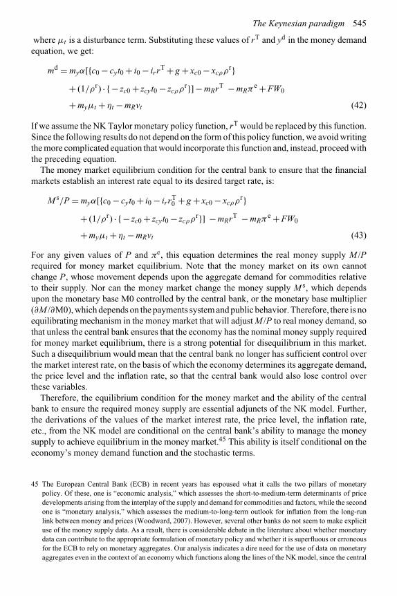
The Keynesian paradigm 545
where μt is a disturbance term. Substituting these values of rT and yd in the money demandequation, we get:
md = myα[{c0 − cyt0 + i0 − irrT + g + xc0 − xcρρr}
+ (1/ρr) · {− zc0 + zcyt0 − zcρρr}]− mRrT − mRπe + FW0
+ myμt +ηt − mRvt (42)
If we assume the NK Taylor monetary policy function, rT would be replaced by this function.Since the following results do not depend on the form of this policy function, we avoid writingthe more complicated equation that would incorporate this function and, instead, proceed withthe preceding equation.
The money market equilibrium condition for the central bank to ensure that the financialmarkets establish an interest rate equal to its desired target rate, is:
M s/P = myα[{c0 − cyt0 + i0 − irrT0 + g + xc0 − xcρρr}
+ (1/ρr) · {− zc0 + zcyt0 − zcρρr}] − mRrT − mRπe + FW0
+ myμt +ηt − mRvt (43)
For any given values of P and πe, this equation determines the real money supply M /Prequired for money market equilibrium. Note that the money market on its own cannotchange P, whose movement depends upon the aggregate demand for commodities relativeto their supply. Nor can the money market change the money supply M s, which dependsupon the monetary base M0 controlled by the central bank, or the monetary base multiplier(∂M /∂M0), which depends on the payments system and public behavior. Therefore, there is noequilibrating mechanism in the money market that will adjust M /P to real money demand, sothat unless the central bank ensures that the economy has the nominal money supply requiredfor money market equilibrium, there is a strong potential for disequilibrium in this market.Such a disequilibrium would mean that the central bank no longer has sufficient control overthe market interest rate, on the basis of which the economy determines its aggregate demand,the price level and the inflation rate, so that the central bank would also lose control overthese variables.
Therefore, the equilibrium condition for the money market and the ability of the centralbank to ensure the required money supply are essential adjuncts of the NK model. Further,the derivations of the values of the market interest rate, the price level, the inflation rate,etc., from the NK model are conditional on the central bank’s ability to manage the moneysupply to achieve equilibrium in the money market.45 This ability is itself conditional on theeconomy’s money demand function and the stochastic terms.
45 The European Central Bank (ECB) in recent years has espoused what it calls the two pillars of monetarypolicy. Of these, one is “economic analysis,” which assesses the short-to-medium-term determinants of pricedevelopments arising from the interplay of the supply and demand for commodities and factors, while the secondone is “monetary analysis,” which assesses the medium-to-long-term outlook for inflation from the long-runlink between money and prices (Woodward, 2007). However, several other banks do not seem to make explicituse of the money supply data. As a result, there is considerable debate in the literature about whether monetarydata can contribute to the appropriate formulation of monetary policy and whether it is superfluous or erroneousfor the ECB to rely on monetary aggregates. Our analysis indicates a dire need for the use of data on monetaryaggregates even in the context of an economy which functions along the lines of the NK model, since the central

546 Monetary policy and the macroeconomy
Taylor-type money supply rules and the relevance of money supply
If the money demand function were stable and all disturbance terms in (43) were equalto zero, substitution of the Taylor rule for the interest rate in the money market equilibriumcondition would yield a money supply function that is itself a type of Taylor rule. For instance,substituting a Taylor interest rate rule of the form:
rTt = r0 +α(yt − yf ) +β(πt −πT) α,β > 0 (44)
for the interest rate in the preceding linear money demand function, yields:
md = myyd +{FW0 − mRπe − mR(r0 +α(yt − yf ) +β(πt −πT))} (45)
so that, for money market equilibrium, the money supply rule would be:
M s = P[myyd +{FW0 − mRπe − mR(r0 +α(yt − yf ) +β(πt −πT))}] (46)
This equation provides the money supply rule that would deliver identical values of theendogenous variables, including the interest rate, under the posited equations for the economy.It is a Taylor-type rule since it makes the money supply a function of the output andinflation “gaps.”
However, if the money demand function is not stable and predictable, the preceding moneysupply rule will have unstable and unknown values of the parameters my and mr , so that thecentral bank will not know the precise amount of money to supply to the economy. Sincethis has been the case in recent decades in economies undergoing considerable financialinnovation, following a money supply rule has proved to be inferior to following an interestrate rule for controlling aggregate demand.
However, this conclusion need not make the money supply redundant for monetary policyif some of the impact of the money supply on output and inflation were independent of interestrates. For the USA, while Rudebusch and Svensson (2002) find support for the redundancyproposition, Nelson (2002) and Hafer et al. (2007) reject such redundancy; money has animpact on output even after controlling for the impact of interest rates on output. Among thereasons offered in Chapter 16 for such a finding is that changes in the money supply couldaffect the cost and amount of credit, which could have an effect on output other than throughinterest rates.
Hence, for the NK model, we conclude that, although monetary aggregates do not appearin the NK model’s equations, the conduct of monetary policy for this model is not merely theselection and pursuit of a Taylor rule for the target interest rate, it also includes the pursuitof an appropriate policy on the relevant monetary aggregates.46 This remains so whetherthe money demand function is stable and known, or not stable and known. The former case
bank needs to ensure the appropriate money supply or face a disconnect between its set interest rate and themarket rate.
46 Therefore, it is erroneous to conclude that “money plays no role in the current consensus macroeconomic modeland in the conduct of monetary policy.” Its erroneous nature can be easily seen if the central bank were to runan experiment that lowers the interest rate but leaves the money supply unchanged or decreases it. In such anexperiment, a disconnect would appear between the central bank’s target rate and the market rate – and theeconomy’s aggregate demand would evolve on the basis of the market rate.
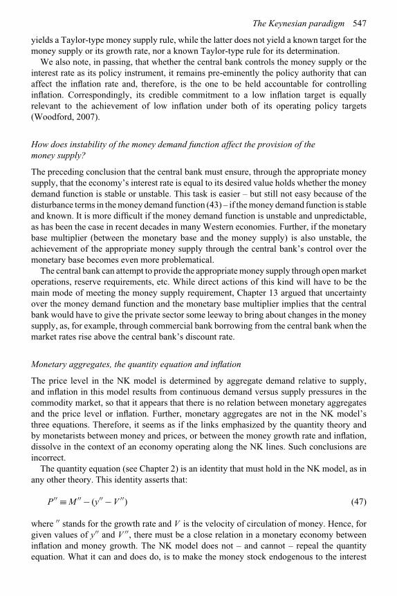
The Keynesian paradigm 547
yields a Taylor-type money supply rule, while the latter does not yield a known target for themoney supply or its growth rate, nor a known Taylor-type rule for its determination.
We also note, in passing, that whether the central bank controls the money supply or theinterest rate as its policy instrument, it remains pre-eminently the policy authority that canaffect the inflation rate and, therefore, is the one to be held accountable for controllinginflation. Correspondingly, its credible commitment to a low inflation target is equallyrelevant to the achievement of low inflation under both of its operating policy targets(Woodford, 2007).
How does instability of the money demand function affect the provision of themoney supply?
The preceding conclusion that the central bank must ensure, through the appropriate moneysupply, that the economy’s interest rate is equal to its desired value holds whether the moneydemand function is stable or unstable. This task is easier – but still not easy because of thedisturbance terms in the money demand function (43) – if the money demand function is stableand known. It is more difficult if the money demand function is unstable and unpredictable,as has been the case in recent decades in many Western economies. Further, if the monetarybase multiplier (between the monetary base and the money supply) is also unstable, theachievement of the appropriate money supply through the central bank’s control over themonetary base becomes even more problematical.
The central bank can attempt to provide the appropriate money supply through open marketoperations, reserve requirements, etc. While direct actions of this kind will have to be themain mode of meeting the money supply requirement, Chapter 13 argued that uncertaintyover the money demand function and the monetary base multiplier implies that the centralbank would have to give the private sector some leeway to bring about changes in the moneysupply, as, for example, through commercial bank borrowing from the central bank when themarket rates rise above the central bank’s discount rate.
Monetary aggregates, the quantity equation and inflation
The price level in the NK model is determined by aggregate demand relative to supply,and inflation in this model results from continuous demand versus supply pressures in thecommodity market, so that it appears that there is no relation between monetary aggregatesand the price level or inflation. Further, monetary aggregates are not in the NK model’sthree equations. Therefore, it seems as if the links emphasized by the quantity theory andby monetarists between money and prices, or between the money growth rate and inflation,dissolve in the context of an economy operating along the NK lines. Such conclusions areincorrect.
The quantity equation (see Chapter 2) is an identity that must hold in the NK model, as inany other theory. This identity asserts that:
P′′ ≡ M ′′ − (y′′ − V ′′) (47)
where ′′ stands for the growth rate and V is the velocity of circulation of money. Hence, forgiven values of y′′ and V ′′, there must be a close relation in a monetary economy betweeninflation and money growth. The NK model does not – and cannot – repeal the quantityequation. What it can and does do, is to make the money stock endogenous to the interest

548 Monetary policy and the macroeconomy
rate target and the price level, with the latter determined by the aggregate demand and supplyof commodities.47 Therefore, the more illuminating form of the quantity equation for the NKmodel is:
M ′′ ≡ P′′ + y′′ − V ′′ (48)
To conclude, the distinctiveness of the NK model does not lie in that it severs the linkbetween the monetary aggregates and the price level or inflation. Its distinctiveness on thislink arises merely from its assumption that the central bank sets an interest rate target, whichoffers a different route for the determination of aggregate demand than a money supply targetpolicy would. The related aspect of its distinctiveness is that the pursuit by the central bankof the interest rate as its monetary policy instrument makes the money supply endogenous tothis interest rate, output and the money demand function. However, the central bank cannotjust ignore the money supply: if it is not to lose control over the market interest rate, it has toensure that the appropriate money supply is provided to the economy.
Note that (48) provides an easier route to the money supply that the central bank needs toprovide: its growth rate has to equal the sum of the inflation rate and the output growth rateless the rate of change of velocity.
15.4.7 NK business cycle theory
The various models of the Keynesian paradigm imply that aggregate demand changes producechanges in output, as do shifts in the production function and labor supply, so that theirexplanations of the business cycle allow both shifts in aggregate demand and supply factorsto be a potential cause of the business cycle. Therefore, from the perspective of monetarypolicy, monetary policy can be potentially a cause of business cycles as well as beinguseful in reducing their severity and duration. In fact, most central banks do habituallymanipulate monetary policy to moderate inflation and the output gap, thereby subscribingto the implication of the Keynesian paradigm that monetary policy can moderate outputand employment fluctuations, as well as maintain inflation within an acceptable range. Thispolicy practice has been confirmed by the estimation of some form of the Taylor rule formany countries over many periods.
New Keynesians base their explanations of business cycles on sticky prices or stickyinflation, as opposed to the flexible price assumption of the real business cycle theory(see Chapter 14). In the NK model, the potential sources of fluctuations in output includeshifts in aggregate demand due to shifts in investment, consumption, exports, fiscal andmonetary policy, etc. Conversely, output fluctuations due to aggregate demand shocks canbe moderated by monetary policy. Further, the new Keynesians’ use of the Taylor rule onthe formulation of monetary policy embeds in monetary policy an automatic stabilizer since,under this rule, an output gap (with actual output below the full-employment level) triggersan expansionary reduction in the interest rate.
Note that once both demand and supply sources of business cycle fluctuations are allowed,their relative importance is likely to vary over different business cycles and for differentcountries. One stance on the explanation of business cycles is the proposition that changes
47 Note that this mode of determination of the price level is shared by the monetarist, neoclassical and Keynesianmacroeconomic models.

The Keynesian paradigm 549
in technology, possibly due to the revolution in information technology (IT), have been thedominant cause of actual business cycle fluctuations in industrialized economies in recentdecades, and that while aggregate demand fluctuations can cause business cycles, they havenot been the dominant source. There does seem to be substantial econometric support for thisproposition.
To provide one illustration out of the many available studies on this topic, Ireland (2001)tests a new Keynesian dynamic, stochastic general equilibrium model of the business cycle forthe USA over the period 1959:1 to 1998:4. His model includes sticky prices (or inflation) andadopts the nominal interest rate as the monetary policy variable, with an additional assumptionon the cost of adjusting physical capital. This study reports that the model performs betterwith costs of adjusting prices rather than inflation. He also finds that persistence in inflationis due more to exogenous real shocks, i.e. to preferences and technology, than to largeadjustment costs.
15.5 Reduced-form equations for output and employment in theKeynesian and neoclassical approaches
The fundamental implication of the various forms of Keynesian models is that, in conditionsof aggregate demand deficiency and less than full employment, aggregate output dependsupon aggregate demand and therefore on the demand management policy variables of fiscalexpenditures, taxation and the money supply. On the impact of monetary policy on realoutput, the Keynesian analyses imply that:
1 This impact will depend upon the existing demand deficiency in the economy, so thata linear relationship between real output and the money supply, with constant coefficients,is not a proper representation of the Keynesian implications.
2 Both the unanticipated and the anticipated values of the money supply – as also of thefiscal variables – will affect output equally, as against the modern classical assertion thatonly the unanticipated values do so.
Keynesian reduced-form equations
A simple linear equation for capturing the dependence of output on the policy variables is:
dy = λg(Dy)dg +λM (Dy)dM λg ≥ 0 (49)
where Dy is the output gap (yf −y), λg and λM are functional symbols, and M is the relevantmonetary policy instrument. λM is non-negative if this instrument is the money supply andnon-positive if it is the interest rate.48 As shown in the preceding sections, λg and λM dependupon the existing demand deficiency in the economy49 and cannot be taken to be constants.
48 In the demand-deficient cases, λg , λM will be non-zero, without being constant, while in the limiting case oflong-run equilibrium (i.e. full employment), λg , λM = 0.
49 This makes them state-contingent, while the Calvo price adjustment process of the NK model makes them time-contingent since, in this process, firms adjust prices on a time schedule, though it is one which is determined bythe economic environment that they face.

550 Monetary policy and the macroeconomy
For a dynamic context, define dy = yt − yt−1, dg = gt − gt−1, dM = Mt − Mt−1, so that(49) becomes:
yt = [yt−1 − (λg(Dyt−1)gt−1 +λM (Dyt−1)Mt−1)]+λg(Dyt−1)gt +λM (Dyt−1)Mt (50)
In line with (50), an equation popular for empirically testing the Keynesian model is:
yt = a0 +λg(Dyt−1)gt +λM (Dyt−1)Mt +μt λg,λM ≥ 0 (51)
where a0 equals [yt−1−(λggt−1+λM Mt−1)],μt is a random term, and all variables are in logs.a0 is sometimes replaced by a term of the form αyt−1 to capture persistent patterns in output,and yt and yt−1 are sometimes defined to be deviations in output from its full-employmentlevel.
Another form of the above Keynesian equation uses the deviation of unemployment fromits natural rate in place of the output gap, and can be specified as:
yt = a0 +λg(ut − unt)gt +λM (ut − un
t)Mt +μt (52)
where u is the unemployment rate, un is the natural (or full-employment) rate of unemploy-ment and λg and λm are functional symbols. λg(ut −un
t) and λM (ut −unt) need not be linear
functions.
Comparison of the NK and modern classical estimating equations
Note that the modern classical equation corresponding to (52) is:
yt = yLR + bg(gt − get) + bM (Mt − Me
t) +μt (53)
where bg , bM > 0 and the superscript e indicates the expected value of the variable in question.In expectational equilibrium with gt = ge
t and Mt = Met , (53) becomes:
yt = yLR +μt (54)
which states the modern classical conclusion that if there are no errors in expectations, theonly deviations around the full-employment output that can occur have to be random ones.
In the modern classical model, since any impact of money supply increases and fiscaldeficits on output must first cause an increase in individual prices or the price level, the moreappropriate equations for testing the modern classical model are:
yt = a0 + γ1(P − EPt) + γPEPt +μt (55)
yt = a0 + γ1(π − Eπt) + γπEπt +μt (56)
where EP and Eπ are the rationally expected values. The equilibrium version of the modernclassical model implies that the estimated values of γP and γπ will be zero, so that monetarypolicy changes will be neutral.

The Keynesian paradigm 551
15.6 Empirical validity of the new Keynesian ideas
One way to judge the empirical validity of the NK model is to compare its implications withthe stylized facts listed in Chapters 1 and 14 on the relationship between money, inflation andoutput. For the long run, the NK model holds that there is no relationship between moneyor inflation and output, as does the modern classical school, so that the stylized short-runfacts are really the relevant ones for judging their relative validity. For the short run, the NKmodel clearly explains more of the stylized facts or does so better than the modern classicalmodel. In particular, it explains the hump-shaped pattern of the impact of monetary changeson output and the longer lag in the impact on money of inflation than on output (Nelson, 1998;Sims, 1992; Christiano et al., 1999). Wong (2000) finds that long-run monetary neutralityand short-run price stickiness hold for the United States. While the NK approach implies anunchanging pattern of impulse responses over time to monetary shocks, Wong finds that theactual responses differ during different episodes and are stronger for negative shocks thanfor positive ones.
Rudd and Whelan (2003) test the forward-looking NK output equation, which asserts thatthe current inflation is positively related to the future output gap. They find that this equationdoes very poorly for US data: empirically, current inflation is negatively, not positively,related to the future output gap. One reason for this poor performance is that there is a highdegree of persistence in inflation, which depends heavily on its own lagged values (see alsoMaria-Dolores and Vazquez, 2006).
The NK school relies on sticky prices and nominal wages for the dynamic impact ofmonetary policy on output. Christiano et al. (2001) find that wage stickiness rather than pricestickiness seems to be the more relevant factor in explaining this dynamic impact. However,Mankiw (2001, p. C52) points out that the NK price adjustment equation based on sticky prices“is completely at odds with the facts. In particular, it cannot come even close to explainingthe dynamic effects of monetary policy on inflation and unemployment.” Mankiw lists threeinvalid implications of the NKPC. One, it implies that a fully credible disinflation causes anincrease in output, since its announcement leads firms to reduce their price increases evenbefore the money supply growth rate is reduced. This causes an increase in the real moneysupply, which leads to higher output and lower unemployment. This is invalid since inflationrises in booms and falls in recessions and the commonly observed result of a decrease inthe money supply is disinflation accompanied by a rise in unemployment. Two, in the NKprice adjustment process, individual prices adjust intermittently so that the price level adjustsslowly to shocks. However, the change in prices as measured by the inflation rate adjustsinstantly, so that the model does not generate persistence in inflation. What is observed inreality is that the impact of a shock to inflation builds up gradually over several quarters, sothere is considerable persistence in inflation. Three, the NKPC does not generate plausibleimpulse response functions in inflation and unemployment following a monetary policyshock. Empirical data shows that a monetary policy shock affects unemployment for sometime after the shock, while the shock has a delayed and gradual effect on inflation. Mankiwconcludes that a backward-looking price adjustment process, with inflation inertia, is neededto explain the observed behavior of inflation.
Many empirical studies find support for some form of the Taylor rule. However, Levin et al.(1999, 2001) report that their estimates from US data for five macroeconomic models showthat a simple version of the inflation and output-targeting rule for the US economy does quitewell. Further, a simple autoregressive model of the interest rate has sometimes performedbetter than the Taylor rule, as Depalo (2006) reports for Japan. Moreover, estimates of the

552 Monetary policy and the macroeconomy
Taylor rule tend to show that its coefficients do shift with changes in the leadership of thecentral bank. This is quite plausible since these coefficients reflect central bank preferences onresponses to inflation and the output gap, etc., as the NK derivation of the Taylor rule shows.
Note that, to derive their particular form of the Taylor rule, NK models assume that the trueforms of the central bank’s objective function and the model are known. These are rarely,if ever, known, so that the superior performance of a specific optimal Taylor rule, derivedfrom a specific model and an objective function, relative to simple Taylor rules, cannot betaken for granted. Given the uncertainty about the future course of the economy and errors inforecasting, it may be better to just specify the central bank’s objectives on inflation, outputand any other targets, while leaving their actual coefficients to vary with the central bank’sappraisal of the circumstances. In this case, the central bank would commit itself only topursuing certain objectives rather than to a set instrument rule such as a specific Taylor rule.Svensson (2003) provides an excellent and detailed discussion of this issue. This conclusionis consistent with that in Chapter 12 on time consistency and credibility: the conclusionthere was that, given uncertainty about the appropriate form of the economy’s constraintsand how they might evolve over time, it might be preferable for the central bank to commititself to objectives in the context of intertemporal reoptimization rather than to a precisetime-consistent path of policies or to a policy rule.
15.7 Conclusions
This chapter has presented three versions of the Keynesian model and a neoKeynesian model.These attest to its evolutionary nature. The future is likely to see additional contributions andversions of the general Keynesian stance that money is not neutral in the short run, while itcould – and is likely to be – neutral in the long run.
We arrange the concluding comments for this chapter into various categories, as follows.
Keynes on the wage bargain and the rigidity of wages
A major point of disagreement between the classical and Keynesian ideas is on the natureof the labor market. Keynes himself considered his objections to the classical model’sassumptions on the labor market as being the most fundamental departures from classicalideas. He expressed his ideas on this as follows:
But the … more fundamental objection [to the classical model] … flows from ourdisputing the assumption that the general level of real wages is directly determinedby the character of the wage bargain. … For there may be no method available to laboras a whole whereby it can bring the wage-goods equivalent of the general level of money-wages into conformity with the marginal disutility of the current volume of employment.There may exist no expedient by which labor as a whole can reduce its real wage to agiven figure by making revised money bargains with the entrepreneurs. …
Though the struggle over money-wages between individuals and groups is oftenbelieved to determine the general level of real wages, it is, in fact, concerned with adifferent object. Since there is imperfect mobility of labor, and wages do not tend toan exact equality of net advantage in different occupations, any individual or group ofindividuals, who consent to a reduction of money-wages relatively to others, will suffera relative reduction in real wages, which is a sufficient justification for them to resistit. On the other hand it would be impracticable to resist every reduction of real wages,
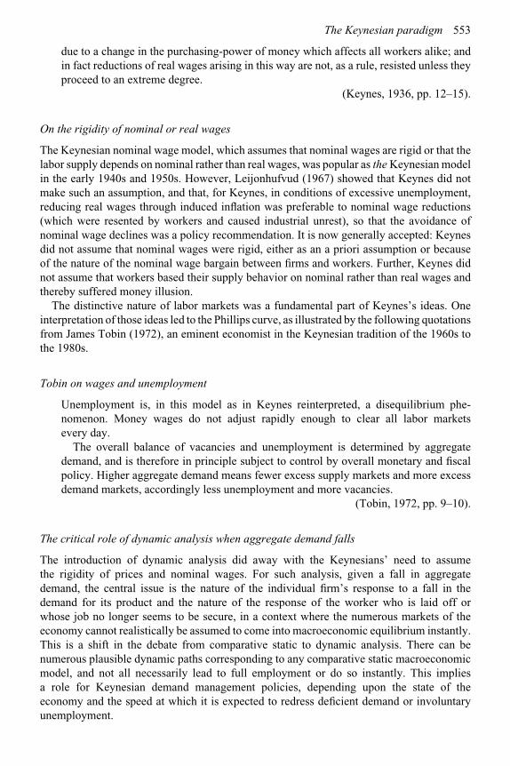
The Keynesian paradigm 553
due to a change in the purchasing-power of money which affects all workers alike; andin fact reductions of real wages arising in this way are not, as a rule, resisted unless theyproceed to an extreme degree.
(Keynes, 1936, pp. 12–15).
On the rigidity of nominal or real wages
The Keynesian nominal wage model, which assumes that nominal wages are rigid or that thelabor supply depends on nominal rather than real wages, was popular as the Keynesian modelin the early 1940s and 1950s. However, Leijonhufvud (1967) showed that Keynes did notmake such an assumption, and that, for Keynes, in conditions of excessive unemployment,reducing real wages through induced inflation was preferable to nominal wage reductions(which were resented by workers and caused industrial unrest), so that the avoidance ofnominal wage declines was a policy recommendation. It is now generally accepted: Keynesdid not assume that nominal wages were rigid, either as an a priori assumption or becauseof the nature of the nominal wage bargain between firms and workers. Further, Keynes didnot assume that workers based their supply behavior on nominal rather than real wages andthereby suffered money illusion.
The distinctive nature of labor markets was a fundamental part of Keynes’s ideas. Oneinterpretation of those ideas led to the Phillips curve, as illustrated by the following quotationsfrom James Tobin (1972), an eminent economist in the Keynesian tradition of the 1960s tothe 1980s.
Tobin on wages and unemployment
Unemployment is, in this model as in Keynes reinterpreted, a disequilibrium phe-nomenon. Money wages do not adjust rapidly enough to clear all labor marketsevery day.
The overall balance of vacancies and unemployment is determined by aggregatedemand, and is therefore in principle subject to control by overall monetary and fiscalpolicy. Higher aggregate demand means fewer excess supply markets and more excessdemand markets, accordingly less unemployment and more vacancies.
(Tobin, 1972, pp. 9–10).
The critical role of dynamic analysis when aggregate demand falls
The introduction of dynamic analysis did away with the Keynesians’ need to assumethe rigidity of prices and nominal wages. For such analysis, given a fall in aggregatedemand, the central issue is the nature of the individual firm’s response to a fall in thedemand for its product and the nature of the response of the worker who is laid off orwhose job no longer seems to be secure, in a context where the numerous markets of theeconomy cannot realistically be assumed to come into macroeconomic equilibrium instantly.This is a shift in the debate from comparative static to dynamic analysis. There can benumerous plausible dynamic paths corresponding to any comparative static macroeconomicmodel, and not all necessarily lead to full employment or do so instantly. This impliesa role for Keynesian demand management policies, depending upon the state of theeconomy and the speed at which it is expected to redress deficient demand or involuntaryunemployment.

554 Monetary policy and the macroeconomy
We illustrate the central issues from this perspective by the following two quotes.
Leijonhufvud on Keynes’s methodology
Keynes’s theory was dynamic. His model was static. The method of trying to analyzedynamic processes with a comparative static analysis apparatus Keynes borrowed fromMarshall. … The initial response to a decline in demand is a quantity adjustment. … Thestrong assumption of “rigid” wages is not necessary to the explanation of such systembehavior. It is sufficient only to give up the equally strong assumption of instantaneousprice adjustments.
(Leijonhufvud, 1967, pp. 401–03; italics added).
Patinkin on effective demand analysis
Involuntary unemployment can have no meaning within the confines of static equilibriumanalysis. Conversely, the essence of dynamic analysis is involuntariness: its domainconsists only of positions off the [notional] demand or supply curves. …
First, we see that involuntary unemployment can exist in a system of perfectcompetition and wage and price flexibility. … Second, we see that a deficiency incommodity demand can generate a decrease in labor input without requiring a priorincrease in the real wage rate.
(Patinkin, 1965, pp. 323–24).
And the assumption … that, granted flexibility, these [dynamic] forces will restore theeconomy to a state of full employment, is an assumption that … [a full employment]equilibrium position always exists and that the economy will always converge to it. Morespecifically, it is an assumption that just as the “market” can solve the system of excessdemand equations (of the neoclassical model), when the level of real income is heldconstant during the tâtonnement, so can it solve it when the level of real income (andhence employment) is also permitted to vary.
(Patinkin, 1965, p. 328).
The points made in these quotes are now generally accepted. Keynes’s analysis wasnot comparative static or Walrasian equilibrium analysis based on the assumption ofinstantaneous market-clearing price adjustments with perfect competition in response toexcess demand or supply, but focused on the dynamic adjustments made by firms when theseconditions did not hold. If the Walrasian market adjustments in prices towards equilibriumwere slow, then, quite plausibly, a shortfall in demand would result in reductions in output andemployment for periods of significant length. If the economy was beset by fresh disturbancesarising frequently, such as through bouts of pessimism or optimism about the future amongfirms’ managers and households, the disequilibrium state would be a persistent phenomenon,with varying levels of employment or output.
NeoKeynesian and new Keynesian economics
NeoKeynesian economics came into being in an attempt to rebuild the Keynesian frameworkafter the decline of faith in the 1970s in the Keynesian models and their policy prescriptions,and the resurgence of classical economics in the 1980s and 1990s. NeoKeynesian economics
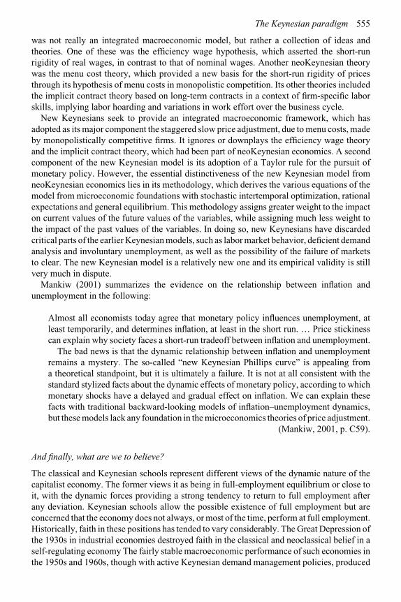
The Keynesian paradigm 555
was not really an integrated macroeconomic model, but rather a collection of ideas andtheories. One of these was the efficiency wage hypothesis, which asserted the short-runrigidity of real wages, in contrast to that of nominal wages. Another neoKeynesian theorywas the menu cost theory, which provided a new basis for the short-run rigidity of pricesthrough its hypothesis of menu costs in monopolistic competition. Its other theories includedthe implicit contract theory based on long-term contracts in a context of firm-specific laborskills, implying labor hoarding and variations in work effort over the business cycle.
New Keynesians seek to provide an integrated macroeconomic framework, which hasadopted as its major component the staggered slow price adjustment, due to menu costs, madeby monopolistically competitive firms. It ignores or downplays the efficiency wage theoryand the implicit contract theory, which had been part of neoKeynesian economics. A secondcomponent of the new Keynesian model is its adoption of a Taylor rule for the pursuit ofmonetary policy. However, the essential distinctiveness of the new Keynesian model fromneoKeynesian economics lies in its methodology, which derives the various equations of themodel from microeconomic foundations with stochastic intertemporal optimization, rationalexpectations and general equilibrium. This methodology assigns greater weight to the impacton current values of the future values of the variables, while assigning much less weight tothe impact of the past values of the variables. In doing so, new Keynesians have discardedcritical parts of the earlier Keynesian models, such as labor market behavior, deficient demandanalysis and involuntary unemployment, as well as the possibility of the failure of marketsto clear. The new Keynesian model is a relatively new one and its empirical validity is stillvery much in dispute.
Mankiw (2001) summarizes the evidence on the relationship between inflation andunemployment in the following:
Almost all economists today agree that monetary policy influences unemployment, atleast temporarily, and determines inflation, at least in the short run. … Price stickinesscan explain why society faces a short-run tradeoff between inflation and unemployment.
The bad news is that the dynamic relationship between inflation and unemploymentremains a mystery. The so-called “new Keynesian Phillips curve” is appealing froma theoretical standpoint, but it is ultimately a failure. It is not at all consistent with thestandard stylized facts about the dynamic effects of monetary policy, according to whichmonetary shocks have a delayed and gradual effect on inflation. We can explain thesefacts with traditional backward-looking models of inflation–unemployment dynamics,but these models lack any foundation in the microeconomics theories of price adjustment.
(Mankiw, 2001, p. C59).
And finally, what are we to believe?
The classical and Keynesian schools represent different views of the dynamic nature of thecapitalist economy. The former views it as being in full-employment equilibrium or close toit, with the dynamic forces providing a strong tendency to return to full employment afterany deviation. Keynesian schools allow the possible existence of full employment but areconcerned that the economy does not always, or most of the time, perform at full employment.Historically, faith in these positions has tended to vary considerably. The Great Depression ofthe 1930s in industrial economies destroyed faith in the classical and neoclassical belief in aself-regulating economy The fairly stable macroeconomic performance of such economies inthe 1950s and 1960s, though with active Keynesian demand management policies, produced

556 Monetary policy and the macroeconomy
shallow and short-lived recessions and led to a slow revival first of classical economics underthe rubric of the Keynesian–neoclassical synthesis. The Keynesian policy errors in the 1970s,resulting in stagflation, tended to restore faith in the general classical position. While thedominant school in the last three decades of the twentieth century seemed to be the classicalone, the Keynesian doctrines, rejuvenated and reformulated, seemed to reclaim dominancetoward the end of the twentieth century. Its currently popular, or rather fashionable, formis that of the NK model, which adopts the market-clearance, general equilibrium, rationalexpectations agenda of the modern classical school, but adds to it market imperfections andsticky prices or information.
The economics profession does not possess empirical evidence sufficient to convinceall economists to accept one paradigm and discard the other, and the performance of theeconomy seems to suit one paradigm at one time and the other one at other times, so thatmany economists keep an open mind, applying their overall knowledge depending upon thestate of the economy. Most economists also maintain a fair degree of skepticism.
Given the uncertainty about the true nature of the macroeconomy and disagreements amongeconomists about the correct workhorse for the economy, the practitioners of monetary policy,the central banks, do not follow a time-invariant commitment strategy to any particularmodel or its implications. Rather, as Chapter 12 argued, they follow a commitment strategyonly with regard to their objectives. In their policies, they follow an active agenda, asthe Keynesians in general recommend, for guiding the short-run evolution of output andemployment through changes in the money supply and/or interest rates, while subscribing tothe classical economists’ belief that monetary policy cannot affect the long-run evolution ofthe real variables.
The current fashion in macroeconomics is to base its foundations strictly and solely onmicroeconomic intertemporal stochastic general equilibrium foundations. The followingquote provides a caution against this practice.
Economists often aspire to make our discipline like physics. Just as there are todaytwo “economicses” – micro and macro … – there are also two “physicses”: quantumtheory, which describes the behavior of the tiniest particles of matter, and Newtonianmechanics (as amended by the theory of relativity), which applies to larger bodies.One of the challenges that physicists face is to integrate the two. As the distinguishedmathematician Roger Penrose has pointed out, however, the way to do it is clearly notsimply to take the principles of quantum theory and apply them wholesale to largerbodies. Doing so leads, in Penrose’s classic example, to concluding that a basketball canbe in two places at once. … Simply applying to aggregate economies what we knowabout the behavior of rational, profit- or utility-maximizing individual agents leads topatent contradictions of the economic world in which we live.
(B.M. Friedman, 2003, p. 10).
Summary of critical conclusions
❖ An abiding theme of the Keynesian paradigm, originating with Keynes’s The GeneralTheory, is the failure of the economy to attain Walrasian general equilibrium. Many ofits models assert that this failure is especially symptomatic of the labor market, so thatinvoluntary unemployment is a common occurrence in real-world economies.
The Keynesian paradigm 557
❖ Early (1940s and 1950s) Keynesian models were based on nominal wage rigidity or priceillusion by labor.
❖ In the 1960s and 1970s, Keynesian models were often based on the Phillips curve.❖ The Keynesian effective demand model posits that the rational dynamic responses by firms
and households to conditions of inadequate demand and involuntary unemployment do notalways take the economy to full employment or do so within an acceptable period.
❖ The neoKeynesian theories rely on rational long-run behavior, resulting in implicitcontracts, staggered wage contracts, sticky prices, menu costs, etc.
❖ The new Keynesians base their macroeconomic model on the microeconomic foundationof forward-looking, optimizing economic agents holding rational expectations and withthe economy operating in general equilibrium. Their distinctiveness from the modernclassical model, which has a similar methodology, lies in that they assume monopolisticallycompetitive firms, sticky prices and the Taylor rule for the central bank’s monetarypolicy.
Review and discussion questions50
1. “In response to demand shocks, short-term quantity adjustments occur earlier thanprice adjustment at the level of both the firm and the economy.” Discuss the relevanttheory behind this statement. Also, discuss its empirical validity at the macroeconomiclevel.
2. Discuss in the context of the effective demand and Phillips curve Keynesian models:excluding dynamic effects, an increase in the stock of money and a fall in nominal wageshave essentially the same effects at a time of involuntary unemployment.
3. Discuss in the context of the neo- and new Keynesian models: excluding dynamic effects,an increase in the stock of money and a fall in nominal wages have essentially the sameeffects at a time of involuntary unemployment.
4. (a) Describe a simple fixed-price short-run macroeconomic model (with flexiblenominal wages) and compare it with a conventional market-clearing model.Compare their predictions for the effectiveness of monetary and fiscal policies.
(b) Describe a simple short-run macroeconomic model with flexible prices but fixednominal wages and compare it with a conventional market-clearing model (withflexible nominal wages). Compare their predictions for the effectiveness of monetaryand fiscal policies.
(c) Describe a simple short-run macroeconomic model with a fixed price and fixednominal wages and compare it with a conventional market-clearing model. Comparetheir predictions for the effectiveness of monetary and fiscal policies.
5. You are given the following fixed-price, closed-economy, IS–LM model:
IS: y = c[(1 − t1)(y + b/r),M + b/r]+ i(r,y) + g
LM : M = md(R,y,M + b/r)
Fisher equation: with an exogenously specified expected inflation rate at zero.
50 Unless a symbol is specifically defined in a question, its definition is as in the text.

558 Monetary policy and the macroeconomy
The government’s budget constraint is:
dM + db/r = g − t1(y + b/r)
where b is the number of consols, each paying $1 per period in perpetuity. P is normalizedto unity. Wealth is held only in money and bonds.
(a) Explain the differences between the IS and LM relationships in this question andthose used in this chapter and Chapter 13.
(b) Explain the government budget constraint.(c) Using IS–LM diagrams, derive the short-run and long-run equilibrium effects on
output of a permanent increase in g financed by (i) money creation, (ii) bond creation.Under what conditions are these policies stable?
(d) How are your results affected if bonds are not part of net wealth?(e) Does this model explain some of the differences between the Monetarists and the
Keynesians on the relative efficacy of monetary versus fiscal policies?
6. Suppose that business pessimism reduces investment such that aggregate demandbecomes less than full employment income at all non-negative rates of interest. UseIS–LM analysis to answer the following:
(a) Are there positive equilibrium levels of y, r and P in the neoclassical model?(b) Are there positive equilibrium levels of y, r and P in the Keynesian fixed-price
model? In the Keynesian nominal wage model (without fixed prices)?
What processes will take the economy to these levels?7. “From the time of Say and Ricardo the classical economists have taught us that the supply
creates its own demand … (and) that an individual act of abstaining from consumptionnecessarily leads to … the commodities thus released … to be invested … so that an actof individual saving inevitably leads to a parallel act of investment … Those who thinkthis way are deceived. They are fallaciously supposing that there is a nexus which unitesdecisions to abstain from consumption with decisions to provide for future consumption,whereas the motives which determine the latter are not linked with the motives whichdetermine the former.” (Keynes, 1936, pp. 18–21). Explain this statement.
If investment and saving depend on different determinants, what are these determinantsand how is the equality of saving and investment in the economy ensured? Or does italso become an identity? If it is not an identity, outline the possible scenario of the likelyadjustment pattern in the economy following an exogenous decrease in consumption.
8. Suppose the central bank pegs the price level by using money supply changes throughopen market operations. Present the IS–LM analysis incorporating this money supplyrule and show the implications for the money supply, aggregate demand and output ofan exogenous increase in autonomous consumption. Is the effect on interest rates less orgreater under this money supply rule than if the money supply were held constant.
9. Start with the neoclassical model and assume that its equilibrium solution is (yf , nf ,r∗, P∗). Suppose a reduction in investment reduces aggregate demand. Discuss thefollowing:
(a) Within the context of the neoclassical model, analyze the behavior of firms if theyface imperfect competition and are hit with a fall in the demand for their products.If this analysis shows that employment is reduced below nf , present the likely
The Keynesian paradigm 559
consumption response of households. If these responses of firms and householdsimply a movement away from (yf , nf , r∗, P∗), what equilibrating mechanisms willcome into play to bring the economy back to (yf , nf , r∗, P∗)? Which do you think ismore powerful and has a faster response: the economy’s equilibrating mechanisms orthe (contrary) responses of firms and households which worked to take the economyaway from (yf , nf , r∗, P∗)?
(b) In the context of a Keynesian model with nominal wage contracting, redo thequestions in (a).
(c) Within the context of a neoKeynesian model, redo the questions in (a).
10. “The classical theory dominates the economic thought, both practical and theoretical,of the governing and academic classes of this generation, as it has for a hundred yearspast. … [But it is] applicable to a special case only and not to a general case, the situationit assumes being a limiting point of the possible positions of equilibrium.” (Keynes,1936, p. 3).
(a) What are the traditional classical (also neoclassical and modern classical) andKeynesian definitions of equilibrium? How are they related? Can there exist anunderemployment equilibrium in their models under each of these definitions?
(b) If you adopt the Keynesian definition of equilibrium, was the traditional classicalmodel a special case of any of the Keynesian models? Of the new Keynesian model?
(c) Are the neoclassical and modern classical models also special cases of any of theKeynesian models?
11. Keynes argued that an economy could be in equilibrium with a substantial amount ofinvoluntary unemployment, but other economists took the stand that an equilibrium inwhich an important market does not clear is a contradiction in terms. Explain the notionsof equilibrium involved, Keynes’s justification for his position, and his opponents’justification for theirs.
12. Distinguish between Keynesian unemployment caused by an aggregate demand defi-ciency and classical unemployment due to real wages being above the full-employmentlevel. What can monetary policy do to reduce each of these?
13. One way of capturing the degree of indexation of nominal wages is by specifying thewage contract as:
W − W0 = α(P − P0) 0 < α < 1
where W0 and P0 are the nominal wage and price levels at the time of the negotiation ofthe wage contract and all variables are in logs. α = 1 indicates full indexation.
Compare the aggregate supply curve when W is indexed to P withα < 1 with the curvesin the fixed nominal wage Keynesian model and the flexible nominal wage neoclassicalmodel. What are the implications of α = 1 for the responsiveness of output and theprice level to (a) aggregate demand shocks, (b) aggregate supply shocks? In this case,would the aggregate supply curve differ from the aggregate supply curve with a flexiblenominal wage?
Show that real output is less sensitive and the price level more sensitive to changes inthe money supply if α is greater.
14. J. R. Hicks, in the 1937 article in which he proposed the IS–LM analysis, argued thatKeynes’s General Theory did not represent a major break with the classical tradition.

560 Monetary policy and the macroeconomy
In particular, he maintained that the main insight it contained was into the conditionsexisting during a depression or a deep recession. Was this claim valid?
Have Keynesians contributed anything further since Keynes’s General Theory? Doesthe above claim apply to the various Keynesian models?
Does the modern classical approach provide an adequate analysis of the economicconditions in recessions and depressions, or does the profession still need the Keynesianapproaches for its analysis?
15. “Keynes argued that wage stickiness was probably a good thing, that wage andprice flexibility could easily be destructive of real economic stability. His reasoningwent like this. In a monetary economy, the nominal interest rate cannot be negative.Hence the real interest rate must be at least equal to the rate of deflation. … Ifwages and prices were to fall freely after a contractionary shock, the real interest ratewould become very large at just the wrong time, with adverse effects on investment.The induced secondary contraction would only worsen the situation.” (Solow, 1980).Discuss the validity of these arguments. Do they apply also to the modern classicalmodel?
16. Keynes (1936) argued that, from a policy perspective, everything that can be achieved bya nominal wage cut can be more effectively achieved through an appropriate monetarypolicy.
(a) Does this statement hold in the deficient-demand Keynesian model for a negativeshock to (i) aggregate demand and (ii) aggregate labor productivity?
(b) Does this statement hold in the new Keynesian model for a negative shock to(i) aggregate demand and (ii) aggregate labor productivity?
17. “Keynesianism and new Keynesianism are fundamentally inconsistent in so far as theirwage hypotheses are concerned. Keynesianism asserts nominal wage rigidity, at leastdownwards, while the new Keynesianism does not allow either nominal or real wagerigidity.” Discuss.
18. In the last two decades of the twentieth century, many economists believed thatKeynesian economics give little or even wrong prescriptions for dealing with thecurrent economic problems in the United States (or British or Canadian) economy. Whatjustifies such comments? What are your views on this issue and how would you justifythem?
19. How does the new Keynesian model differ from the earlier Keynesian deficient-demandmodel? How does it differ from the modern classical one? Which of the three modelswould explain involuntary unemployment in a recession following a fall in aggregatedemand?
20. “Every major inflation has been produced by monetary expansion” (Friedman, 1968).Does this assertion hold for the NK model, whose equations do not even include amonetary aggregate as a variable?
21. “Because monetary shocks have a delayed and gradual impact on inflation, in essence weexperience a credible announced disinflation every time we get a contractionary shock.Yet we don’t get the boom that the (new Keynesian) model says should accompany it.This means that something is fundamentally wrong with this model.” Discuss the validityof the preceding observation. In particular, is this observation valid for contractions inmonetary policy that were unanticipated when the policy was first announced? Whatdoes the new Keynesian model imply on this issue? If it is fundamentally wrong, howmight the new Keynesian model be modified to fit the facts?
The Keynesian paradigm 561
22. “It is now well established that a contractionary monetary shock increases unemploymentbefore reducing inflation and that the peak impact on unemployment precedes the peakimpact on inflation.” Discuss how well these observations are explained by (i) the modernclassical model, (b) the new Keynesian model, and (c) any one other Keynesian modelof your choice.
References
Ball, L., Mankiw, N.G. and Romer, D. “The new Keynesian economics and the output–inflationtrade-off.” Brookings Papers on Economic Activity, 19, 1988, pp. 1–65.
Blanchard, O. “What do we know about macroeconomics that Fisher and Wicksell did not?” QuarterlyJournal of Economics, 65, 2000, pp. 1375–409.
Boschen, J.F. and Weise, C.L. “What starts inflation: evidence from the OECD countries.” Journal ofMoney, Credit and Banking, 35, 2003, pp. 323–49.
Calvo, G. “Staggered prices in a utility maximizing framework.” Journal of Monetary Economics, 12,1983, pp. 383–98.
Christiano, L.J., Eichenbaum, M. and Evans, C. “Monetary policy shocks: what have we learned and towhat end?” In J. Taylor and M. Woodford, eds, Handbook of Macroeconomics, Vol. 1A. Amsterdam:Elsevier North-Holland, 1999, pp. 65–148.
Christiano, L.J., Eichenbaum, M. and Evans, C. “Nominal rigidities and the dynamic effects of a shockto monetary policy.” NBER Working Paper no. 8403, 2001.
Clarida, R., Gali, J. and Gertler, M. “The science of monetary policy: a new Keynesian perspective.”Journal of Economic Literature, 37, 1999, pp. 1661–707.
Clarida, R., Gali, J. and Gertler, M. “Monetary policy rules and macroeconomic stability: evidence andsome theory.” Quarterly Journal of Economics, 115, 2000, pp. 147–80.
Clower, R. “The Keynesian counter-revolution: a theoretical appraisal.” In F.H. Hahn andF.P.R. Brechling, eds, The Theory of Interest Rates. London: Macmillan, 1965.
Depalo, D. “Japan: the case for a Taylor rule? A simple approach.” Pacific Economic Review, 11, 2006,pp. 527–46.
Eichenbaum, M. and Fisher, J.D.M. “Estimating the frequency of price re-optimization in Calvo-stylemodels.” Journal of Monetary Economics, 54, 2007, pp. 2032–47.
Friedman, B.M. “The LM curve: a not-so-fond farewell.” NBER Working Paper no. 10123, 2003.Friedman, M. “The role of monetary policy.” American Economic Review, 58, 1968, pp. 1–17. Reprinted
in Milton Friedman, The Optimum Quantity of Money and Other Essays. Chicago: Aldine PublishingCo. 1969, p. 106.
Gali, J. “New perspectives on monetary policy, inflation and the business cycle.” NBER Working Paperno. 8767, 2002.
Galí, J. and Gertler, M. “Inflation dynamics: a structural econometric analysis.” Journal of MonetaryEconomics, 44, 1999, pp. 195–222.
Hafer, R.W., Haslag, J.H. and Jones, G. “On money and output: Is money redundant?” Journal ofMonetary Economics, 54, 2007, pp. 945–54.
Handa, J. Monetary Economics. London, Routledge, 2000.Hicks, J.R. “Mr. Keynes and the classics: a suggested interpretation.” Econometrica, 5, 1937,
pp. 147–59.Ireland, P.N. “Sticky-price models of the business cycle: specification and stability.” Journal of
Monetary Economics, 47, 2001, pp. 3–18.Keynes, J.M. A Tract on Monetary Reform. London: Macmillan, 1923.Keynes, J.M. The General Theory of Employment, Interest and Money. New York: Macmillan, 1936.Leijonhufvud, A. “Keynes and the Keynesians.” American Economic Review, Papers and Proceedings,
57, May 1967, pp. 401–10.Leijonhufvud, A. On Keynesian Economics and the Economics of Keynes. New York: Oxford
University Press, 1968.

562 Monetary policy and the macroeconomy
Levin, A., Wieland, V. and Williams, J.C. “Robustness of simple monetary policy rules under modeluncertainty.” In J.B. Taylor, ed., Monetary Policy Rules. Chicago: University of Chicago Press,1999, pp. 263–99.
Levin, A., Wieland, V. and Williams, J.C. “The performance of forecast-based monetary policy rulesunder model uncertainty.” Working Paper 2001-39, Board of Governors of the Federal ReserveSystem, 2001.
Mankiw, N.G. “The inexorable and mysterious tradeoff between inflation and unemployment.”Economic Journal, 111, 2001, pp. C45–C61.
Mankiw, N.G. “Pervasive stickiness.” American Economic Review, 96, 2006a, pp. 164–9.Mankiw, N.G. “Sticky information in general equilibrium.” NBER Working Paper no. 12605, 2006b.Mankiw, N.G. and Reis, R. “Sticky information versus sticky prices: a proposal to replace the new
Keynesian Phillips curve. Quarterly Journal of Economics, 117, 2002, pp. 1295–328.Maria-Dolores, R. and Vazquez, J. “How does the new Keynesian monetary model fit in the U.S. and the
Eurozone? An indirect inference approach.” Topics in Macroeconomics, 6, 2006, article 9, pp. 1–49.Nelson, E. “Sluggish inflation and optimising models of the business cycle.” Journal of Monetary
Economics, 42, 1998, pp. 302–22.Nelson, E. “Direct effects of base money on aggregate demand: theory and evidence.” Journal of
Monetary Economics, 49, 2002, pp. 687–708.Okun, A. Prices and Quantities: A Macroeconomic Analysis. Washington DC: Brookings Institution,
1981.Patinkin, D. Money, Interest and Prices. New York: Harper and Row, 1965.Phillips, A.W. “The relation between unemployment and the rate of change of the money wage rates
in the U.K. 1861–1957.” Economica, 25, 1958, pp. 283–99.Rotemberg, J. and Woodford, M. “Interest rate rules in an estimated sticky price model.” In J.B. Taylor,
ed., Monetary Policy Rules. Chicago: University of Chicago Press, 1999.Rudd, J. and Whelan, K. “Can rational expectations sticky price models explain inflation dynamics.”
at www.federalreserve.gov/pubs/feds/2003/200346, 2003.Rudebusch, G.D. “Federal reserve interest rate targeting, rational expectations and the term structure.”
Journal of Monetary Economics, 35, 1995, pp. 245–74.Rudebusch, G.D. and Svensson, L.E.O. “Eurosystem monetary targeting: lessons from US data.”
European Economic Review, 46, 2002, pp. 417–42.Shapiro, C. and Stiglitz, J.E. “Equilibrium unemployment as a worker discipline device.” American
Economic Review, 74, 1984, pp. 433–44.Sims, C.A. “Interpreting the time series facts: the effects of monetary policy.” European Economic
Review, 36, 1992, pp. 975–1000.Solow, R. “On theories of unemployment.” American Economic Review, 70, 1980, pp. 1–11.Svensson, L.E.O. “What is wrong with Taylor rules? Using judgment in monetary policy through
targeting rules.” Journal of Economic Literature, 41, 2003, pp. 426–77.Taylor, J.B. “Discretion versus policy rules in practise.” Carnegie-Rochester Conference Series on
Public Policy, 39, 1993, pp. 195–215.Tobin, J. “Inflation and unemployment.” American Economic Review, 62, 1972, pp. 1–18.Walsh, C. Monetary Theory and Policy, 2nd edn. Cambridge, MA: MIT Press, 2003.Wong, K. “Variability in the effects of monetary policy on economic policy.” Journal of Money, Credit,
and Banking, 32, 2000, pp. 179–98.Woodford, M. “How important is money in the conduct of monetary policy?” NBER Working Paper
no. 13325, 2007.Yellen, J.L. “Efficiency wage models of unemployment.” American Economic Review, 74, 1984,
pp. 200–5.

16 Money, bonds and credit in macromodeling
For the short-run macroeconomic analysis, this chapter differentiates between two types of non-monetary financial assets: bonds and credit, of which bonds are long-term financial instrumentsand credit represents short-term assets. The distinctive aspect of credit relies upon adverseselection, moral hazard, and monitoring and agency costs, which provide a basis for creditrationing in quantity. Credit is treated in this chapter as the variable element of working capitalin the short-run. The distinctive impact of credit on economic activity is designated the creditchannel.
An important element of credit is bank loans. The distinctive impact of bank loans oneconomic activity occurs through the bank lending channel.
Key concepts introduced in this chapter
♦ Adverse selection♦ Moral hazard♦ Monitoring and agency costs♦ Credit versus bonds♦ Credit rationing♦ Credit market equilibrium♦ Bank loans♦ Working capital♦ Indirect production function
The IS–LM and IS–IRT models belong to a context that assumes perfect substitution amongnon-monetary financial assets, which means that all non-monetary assets, as well as theirdifferent types, are perfect substitutes, so that the distinctive elements of bonds, stocksand loans, as well as the distinctions between short- and long-term bonds, government andcorporate bonds, etc., can be omitted from the analysis, and all such assets can be encompassedin a composite financial asset which is labeled “bonds.” Hence, the assumption of perfectfinancial markets leaves the macroeconomic model with only two financial assets, money(which functions as a medium of payments) and bonds (which do not), and only two financial

564 Monetary policy and the macroeconomy
markets, which are the markets for money and bonds.1 In the case where the central banksets the money supply, the money market is specified by the LM equation (see Chapter 13).In the standard IS–LM analysis, an increase in the money supply decreases the interest rateon bonds, which increases investment and aggregate demand.
The extension of the perfect markets (i.e. perfect competition, perfect information andmarket efficiency) hypothesis to non-monetary financial assets implies the irrelevance ofthe composition of financial assets in firms’ and households’ portfolios and liabilities. Forsuch a scenario, Modigliani and Miller (1958) provided the Modigliani–Miller theorem,which showed that, under perfect markets and ignoring differential tax treatments, the firm’scombination of bond and equity financing was irrelevant to its output and employment, aswell as to its profits which would depend on technology, inputs and consumer tastes. Further,Fama (1980) showed that whether the public holds money, bonds or stocks is irrelevant to realeconomic outcomes, which depend only on technology, tastes and resources. Hence, underthe perfect financial markets hypothesis, financial assets and their distinctive characteristicswere irrelevant for the real variables of the economy and there was no need to separate theminto money, bonds, stocks, loans, etc. An intuitively unrealistic implication of these results isthat credit crunches2 and bank panics/runs3 would have no impact on output and employment,even though such impact is often observed in recessions.4
As against the assumption of perfect markets, the central theme of neoKeynesian andnew Keynesian economics is market imperfections.5 Applied to financial markets, marketimperfections between bonds, stocks and loans imply that they are not perfect substitutesfor each other since each has quite distinctive characteristics. Further, each of theseassets has many distinctive sub-categories. For example, among bonds there are short-term and long-term bonds, and there are low-risk bonds issued by some governments andhigh-risk ones issued by some corporations. Therefore, an extreme emphasis on marketimperfections would lead to the consideration of very many different non-monetary financialassets.
However, aggregation is essential to macroeconomics, so that it needs to use the smallestnumber of composite goods that will adequately explain the desired macroeconomic aspectsof the economy. For financial assets, the general consensus until about the 1980s was thattwo composite assets, money and bonds, are adequate for explaining the impact of monetary
1 In the limiting case, the assumption of perfect markets, combined with perfectly competitive and efficient markets,implies the neutrality of both money and bonds, so that all financial assets become irrelevant to the determinationof output and employment.
2 A credit crunch is a sharp decline in the supply of credit, especially bank loans.3 A bank panic or run is characterized by a strong shift in the desired currency/deposit ratio of depositors.4 An illustration of this comes from explanations of recessions and depressions. In the context of the Great
Depression of the 1930s, under the implications of perfect markets, money and shifts in the financial structurewould have no impact on real variables, so that the Great Depression would have been solely due to real causes,as specified in the real business cycle theory. Further, models that allow money non-neutrality, but in whichall non-monetary assets are identical, explain the monetary contribution to the Great Depression by citing onlydecreases in the money supply due to the collapse of the banking system as a cause or contributory factor, butotherwise deny credit shortages any role. The financial imperfections hypothesis uses both the decrease in themoney supply and the credit restrictions and shortages among the causes of the Great Depression and its duration.There is now significant empirical evidence to support this position.
5 Information imperfections that lead to special financial arrangements for some borrowers, such as in the form ofloans rather than bonds, imply that the structure of the financial system determines the sources and uses of fundsand can affect real outcomes in the economy.
Money, bonds and credit 565
policy on output and prices/inflation. However, some economists, especially new Keynesians,now believe that because of significant information imperfections a classification of financialassets into three or more assets can explain some monetary policy effects that are not wellexplained by the two-asset, money and bonds, classification. This chapter examines thisissue and specifies a macroeconomic model with money, bonds and credit, which is defined toinclude loans. Its emphasis on imperfections in financial markets leads to models with a creditchannel, in addition to the bond interest rate channel of the transmission of monetary policyon aggregate demand. In some models, information imperfections lead to credit rationing(Stiglitz and Weiss, 1981).
For intuition, it would be useful first to review the main characteristics of the non-monetaryfinancial assets in the economy. Bonds in the real-world financial markets are marketablein both primary and secondary markets and their buyers and sellers incur brokerage costs.Marketed bonds do not need any specific collateral, other than the assets of the firm if it wereto become bankrupt, nor do they need the credit-worthiness of the issuer of the bond to beestablished on a one-to-one basis. In terms of the returns on them, their coupon payments andmaturity dates are set when they are issued and their price at their maturity date is known inadvance. Bonds can be long-term or short-term. The latter, when issued by firms, are called“commercial paper.”
A useful definition of credit is short-term debt, including loans of various types, whichneeds to be rolled over after a short period, so that its amount can be taken to be variable duringthe short-run. This definition places commercial paper, along with loans and trade credit,among the components of credit. In line with this definition, this chapter defines “bonds”as marketable debt instruments other than commercial paper of firms, and all bonds issuedby the government. Of the components of credit, bank loans (including lines of credit) aremade directly to customers by financial institutions6 (designated in this chapter as “banks”)and trade credit is extended by firms directly to their customers. More so than bonds, loansand trade credit depend on the direct (as opposed to market) evaluation by the lender of thecredit-worthiness of the borrower, which is determined from the individual circumstances ofthe borrower as well as the state of the markets and the economy.
In general, borrowing through credit can be arranged at short notice and the terms of someof the credit are such that they can be repaid by the borrower or recalled by the lender atany time.7 Often, for bank loans and trade credit, the credit interest rate is adjustable bythe lender even during the duration that the loan is held. The coupon rate on short-termcommercial paper gets adjusted at maturity, which occurs only a short period after its issue.As compared with this short-term variability, the coupon on medium- and long-term bondscannot be adjusted until their maturity, which does not occur for quite some time aftertheir issue. Although the demand for such bonds can fall, this triggers an increase in theiryield in the secondary bond markets, but neither the pre-set time pattern of the coupon ratepromised by the issuer nor the amount made available to the issuer usually changes until theirmaturity.
To create a strong analytical distinction between bonds and credit, this chapter assumesthat these adjustments in the coupon rate and the amount lent through bonds can occur in the
6 Kashyap and Stein (1994) show that banks in the USA dominate loan financing and the financing of small andmedium-sized firms.
7 Given this feature, for loans, the lender can re-assess the credit-worthiness of the borrower at any time and reduceor recall the loan or ask for additional collateral.
566 Monetary policy and the macroeconomy
long-run but not in the short-run, so that the amount of funds available to firms from bondissues is given for short-run macroeconomic analysis. By comparison, our assumption is thatboth the amount of credit (including loans and commercial paper) made available to firmsand the credit interest rate can be varied in the short-run. In terms of correspondence with thereal-world financing arrangements, the preceding strong distinction provides some guidanceon where different types of bonds should be slotted. Since our concern is with credit to theprivate sector, short-term corporate bonds8 (“commercial paper,” including “finance paper”)need to be slotted in “credit,” along with the loans made directly by banks to firms, sinceboth provide short-term financing to firms and their interest cost to the issuer is frequentlyadjustable. Hence, short-run variability in the quantity and cost to the private sector is ourbasis for the distinction between credit and bonds, not marketability versus non-marketability;commercial paper is marketable whereas loans are not, but both are being slotted in credit.Therefore, our analytical concept of credit includes loans and short-term corporate bonds,but not longer-term bonds or government bonds. By implication, our analytical concept ofbonds only includes medium- and long-term marketed corporate bonds and all governmentbonds.
Looking now at stocks, stocks/equities in the real-world financial markets do not have amaturity date and most types of stocks do not promise any coupon payment. Existing stockscan only be traded in the secondary/stock market at a price that continually fluctuates. Sincetheir price depends on the expectation of uncertain future dividends, themselves dependenton the uncertain profitability of the firm issuing them, their yield usually has a higher degreeof uncertainty than bonds, which have pre-specified coupon payments and a maturity date,and loans. However, unlike loans, stocks do share with bonds the characteristic that they donot need any collateral up front, nor do they need the credit-worthiness of the issuer to beestablished on a one-to-one basis.
Given these differences, one could argue that macroeconomic models need to treat money,credit, bonds and stocks as distinct financial assets in the sense that no pair has perfectsubstitution, so that the overall macroeconomic model needs to have three non-monetaryassets and their three rates of return. However, doing so increases the analytical complexityof the macroeconomic analysis beyond the simplicity of the IS–LM or IS–IRT models, whichhave only one non-monetary financial asset and only one rate of return, so that convincingreasons in terms of the relative impact of shifts in the bonds, loans and stock markets onthe economy have to be provided to justify the extension of the macroeconomic model toincorporate three non-monetary financial assets.
This chapter follows other studies that incorporate financial imperfections in limiting theclassification of financial assets to just three assets, money, bonds and credit, with stocks stilllumped in bonds, and builds a simple form of the macroeconomic model incorporating thesethree assets. Among several good reviews on the credit channel are Bernanke (1992–93),Kashyap and Stein (1993, 1997), Hubbard (1995), Bernanke et al. (1999) and Walsh(2003, Ch. 7).
Note that Walras’s law allows one of the markets to be omitted from explicit analysis.Following the usual convention in the IS–LM and IS–IRT analyses, this chapter omits theexplicit analysis of the bond market, so that the financial markets explicitly analyzed will bethose of money and credit.
8 Some types of such bonds (asset-backed bonds) require backing by other securities, which serve as collateral,which is also often needed for loans.
Money, bonds and credit 567
For aggregate demand in the macroeconomic model, this chapter draws on the model inBernanke and Blinder (1988) for the supply of loanable funds.9 For the aggregate supply ofcommodities, this chapter relies on the indirect production function, in which working capitalbecomes an input, along with labor and physical capital in production, with physical capitaltaken to be fixed in the short-run, as in the usual textbook AS–AD model. Workingcapital plays the role of an input in a monetary economy by facilitating the purchases ofinputs (including labor, raw materials and intermediate goods) and allowing the revenuefrom sales to accrue to the firm with a lag. This chapter adopts the plausible hypothesis thatworking capital can vary in the short-run. Since working capital is an input in the indirectproduction function, a decrease in it reduces the purchases of labor and other inputs, andthereby reduces output.10
Working capital
Working capital includes all funds that the firm uses to facilitate its purchases of inputs andproduction, and sales of its output. The firm may obtain its working capital from its retainedearnings, equity issues, bond issues and loans (including the use of overdrafts or lines ofcredit) – or save on the need for working capital by arranging trade credit. In the long-run,the firm can vary each of the sources of working capital. However, for the short-run analysis,the amount of working capital prearranged by the firm through its retained earnings and issueof bonds (including equities) is taken to be predetermined11 and not variable. Hence, for theshort-run of our model, the only component of working capital that is allowed to vary is thatobtained through credit.12
Motivating the analysis of the credit market
The study of the money and financial markets would be irrelevant for the determination ofoutput, employment and other real variables if money and non-monetary financial assets wereneutral. While such a proposition is implicitly held by virtually all macroeconomic models forthe hypothetical, analytical long-run, few macroeconomic models imply it for the short-run,especially in the context of uncertainty, adjustment costs and imperfect competition. In fact,the short-term behavior of the economy is clearly such as to convince the public, economicanalysts, central bankers and governments that movements in money and credit, and notmerely their unanticipated components, alter output and employment. This can be clearlyseen from the very active pursuit of monetary policy by many central banks to stabilize theeconomy’s output around its long-run growth path. It is also obvious from the declines in
9 Bernanke and Blinder provide a commonly used macroeconomic model with money, bonds and loans asfinancial assets. However, their analysis focuses only on the aggregate demand for output. Kiyotaki and Moore(1997) present another loan-based model intended to explain credit cycles. Their models, along with others, aresummarized in Walsh (2003, Ch. 7).
10 The asset-backed commercial paper crisis in USA in 2007 illustrates this role extremely well. Cutbacks inthe amount made available in this market meant a severe tightening of credit, with a subsequent cutback inproduction.
11 Remember, bonds in our model have been defined to exclude issues of commercial paper as a way ofsupplementing working capital in the short-run.
12 Kashyap et al. (1993) and Gertler and Gilchrist (1994) found that commercial paper issuance by large firmsexpanded during periods of tight credit while those by small firms declined, which represents a flight to quality(i.e. to lower risk loans) by the lenders.
568 Monetary policy and the macroeconomy
output and rises in unemployment caused by currency, credit and exchange crises.13 Moneyand credit are, therefore, definitely not neutral in the short-run.14 This needs to be reflectedby the macroeconomic models. The IS–LM and IS–IRT models, at best, do this job poorlyand need to be modified to achieve more realistic implications on the impact of a shortageof credit on production. That is, the effects of credit are mainly due to variations in its total,rather than to changes in its composition.
Definitions of credit and loans
If we accept that credit should be treated as distinct from bonds, what should be its definitionfor macroeconomic analysis? Should it be defined as synonymous with bank loans, as in muchof the literature on this topic? We choose to define it as all short-term loans to the privatesector, whether marketable or not. As such, its major components are trade credit (providedby suppliers of commodities to buyers), short-term corporate bonds, and loans by banksand other lenders. Therefore, under our definition of credit, loans are just one component ofcredit.
Our choice of credit rather than merely loans as the distinctive non-monetary financial assetis partly due to our emphasis on credit as the variable component of working capital in theshort-run and the impact of variations in it on the production of commodities. Another reasonis our belief that information imperfections, discussed in the next section, which are usuallybehind the treatment of loans as a distinctive financial asset, really affect all financial assets,including trade capital, short-term bonds and long-term bonds, rather than merely loans.Admittedly, banks, when making loans on a personal basis, cope with market imperfections ina different way to financial markets, but our belief is that this difference is less important thanthat between short-run variability (for all forms of credit) versus non-variability (for bonds),which is what is needed to distinguish between short-run and long-run effects. Further, tradecredit and bank loans suffer in a very similar fashion from market imperfections. In addition,an advantage of including bank loans, trade credit and commercial paper within the singlecategory of credit is that if changes in one of them offset to some extent changes in another,only the net change in the total becomes relevant for the analysis.15
In any case, if one chooses, credit can be replaced by loans in this chapter, without changingthe gist of its arguments.
Links between credit and economic activity and between credit and monetarypolicy: lessons of the 2007 subprime asset crisis for macroeconomic analysis
The 2007 crisis in the subprime asset-backed credit market (ABCM) in the USA, and itsimpact on housing construction and real economic activity generally in the USA and the
13 To illustrate, in 2007, during the crisis in the subprime financial markets, speeches and reports on its impact oneconomic activity often carried headings such as “Heading for the rocks: will financial turmoil sink the worldeconomy?”
14 Their non-neutrality was starkly illustrated during the subprime mortgage crisis in the USA during 2007, whenthe reappraisal of risk on mortgage-backed securities led to the drying up of the demand for short-term securitiesby financial institutions and caused fears that the shortage of working capital would lead to cutbacks in productionand a recession in the US economy, and in the world economy.
15 Several studies report that a tightening of bank loans leads to an increase in commercial paper issued by largerfirms.

Money, bonds and credit 569
world, illustrates how shifts in the availability of credit affect real economic activity andhow the availability of money affects that of credit, so that neither credit nor money isneutral for real economic activity. House prices in the USA had shot up during 2001 to2006 to such an extent that the rise was generally considered to be a bubble. This risehad been prompted by shifts in investment after the collapse of stock prices due to thecrash in Internet stocks in 2001–02, and by exceptionally low interest rates during 2001 to2006. As house prices rose, the demand for housing was further boosted by the practiceof mortgage lenders to ease the terms for obtaining mortgages: some mortgages were for100 percent of the purchase price of a house, even to customers who did not have theincome to cover the projected monthly mortgage payments. This practice did not pose aserious problem as long as house prices continued to rise sufficiently fast, since the priceincrease provided a cushion for both buyers and lenders. However, house prices beganto stabilize and then to fall in 2006. Further, interest rates began to rise. The result wasan increase in mortgage defaults and a heightened perception of the riskiness of suchmortgages.
Collections of the initial mortgages and other credit, such as installment credit on purchasesof cars, were bundled into marketable securities, with the former serving as collateral for thelatter. The securities usually had terms of 30 to 60 days, similar to that on Treasury bills, andwere called asset-backed commercial paper. Since they carried a higher yield than Treasurybills but seemed to be equally liquid and safe investments, they proved attractive to manylenders as a component of their portfolios. They were bought by (production) firms, as well asby commercial and investment banks, etc. Once house prices in the USA began to fall and therisks of mortgage default rose, the riskiness and eventually illiquidity of such asset-backedcommercial paper became apparent, so that the demand for them fell drastically, while theinterest rates on them rose. With many issuers of such bonds unable to roll them over, therisk of default in this market rose significantly. This reduced the flow of funds for workingcapital to firms, affecting their production. The possibility of such a default also affectedthe holders of such securities, reducing their liquidity and profitability. Since many banksand other firms in the USA and many other countries held such securities, the crisis in thesubprime (high-risk) market threatened to become a general financial crisis, which in turnthreatened to deplete the amount of working capital for firms in production and send the USAand the world economies into a recession.
The subprime crisis could be viewed as one of the short-run liquidity, rather than long-term solvency, of most financial institutions holding the mortgage-backed securities. Aspart of attempts to limit the impact of the subprime crisis, central banks in the USA,Europe and other affected countries pursued an aggressive expansionary monetary policyby increasing the money supply through open market operations, cutting discount rates andopenly calling for commercial banks to borrow funds as needed from the central bank.In the USA, the Fed increased the money supply very significantly, cut its discount rateby 1 percent (and openly encouraged bank borrowing at this rate), following this by a cutin the federal funds rate by ½ percent, with subsequent cuts occurring gradually. In spiteof the aggressive actions taken by several central banks, the fallout of the subprime crisisfor real economic activity remained uncertain for quite some time: while the projectionsof the real growth rates of the world economy were cut, such a reduction was nominalfor the optimistic scenarios and drastic for the pessimistic ones, with the latter forecastinga severe world recession. However, it was soon clear that, by reducing the workingcapital of firms, the subprime crisis had the potential to cause a recession in output andthat aggressive expansionary monetary policy did moderate but not eliminate this effect.

570 Monetary policy and the macroeconomy
The day-by-day and week-by-week pronouncements of central banks and economic analystsduring this period did also highlight the very considerable uncertainty of the extent of theneed for monetary policy and the difficulty of formulating the appropriate policy in a timelyfashion.
Briefly, firms habitually rely on credit to conduct their production, so that a credit crisis,by reducing the credit made available to firms, is likely to reduce their production in theshort-run. If the credit markets do not provide the needed liquidity in sufficient amountsand in a timely manner, a credit crisis tends to evolve into an economic one, in which theeconomy goes into a recession. The standard IS–LM, AD–AS model does not provide a linkfrom credit to production, so the subprime crisis cannot be explained by using it. This chaptertries to provide a model that links credit to the production activities of firms and also linkscredit to the money supply.
16.1 Distinctiveness of credit from bonds
16.1.1 Information imperfections in financial markets
The information that borrowers and lenders bring to their exchanges and the ability ofborrowers to change the probability of default play an important role in the nature of creditcontracts, the ability of credit markets to match borrowers and lenders, and the role playedby the interest rate and credit rationing in the allocation of credit among borrowers. Giventhat there is a risk of default by a borrower, risk-averse lenders base their decision to lend onthe expected return while borrowers need only base their decision to borrow on the interestrate that they have to pay. While the terms of the loan usually guarantee the latter, they donot guarantee the probability of not defaulting. Credit-rationing models imply that lenderswill not raise interest rates beyond the point at which their expected return begins to decline,even though some (higher risk) borrowers are willing to pay higher interest rates (Jaffee andRussell, 1976; Stiglitz and Weiss, 1981). In this case, the credit market “equilibrium” wouldbe characterized by an excess demand for credit, so that there would be quantity rationing(through the amount lent), in addition to price rationing through the interest rate.
“Credit rationing” occurs if, at the going interest rate, lenders supply a smaller amount thanthe borrowers want to obtain. In addition, among borrowers willing to pay the going interestrate, some borrowers receive credit while others do not. In fact, the latter may be willing topay a higher interest rate but may still not get the credit. Hence, there is an unsatisfied demandfor credit that is not eliminated by a rise in the interest rate. Consequently, equilibrium in thecredit market is characterized by the equilibrium interest rate and credit rationing (Jaffee andStiglitz, 1990; Stiglitz and Weiss, 1981).
Information imperfections16 in financial markets occur because of adverse selection, moralhazard, and monitoring and agency costs – and because of the undeveloped and segmentednature of the financial sector of some economies. Under uncertainty, different borrowers canhave different probabilities of repayment (versus default). If the lender can observe these
16 Akerlof (1970) illustrated the role of information imperfections in the used car market by assuming that usedcar sellers know the quality of the car but buyers do not. The latter view lower prices set by sellers as indicativeof poorer quality, so that lowering the price does not increase demand. Therefore, in the used car market, anexcess supply of cars need not be cleared by a lower price. In fact, there may be no price at which supply equalsdemand.
Money, bonds and credit 571
probabilities and if they are not affected by the decision to lend, lenders can accuratelyrank the borrowers on the basis of their expected return and make loans to those who willyield the highest expected return. In practice, lenders cannot actually observe the borrower’sprobability of repayment or rely upon this probability remaining invariant. To illustrate, startwith equilibrium in the credit market at the current expected return and assume that thereis an unsatisfied demand by borrowers at this equilibrium. Given this unsatisfied demand atthe equilibrium interest rate, suppose that the lenders were to increase the interest rate. Atthe higher rate, some borrowers, including those with less risky projects, might no longerfind it profitable to borrow, while those with riskier projects may still be willing to borrow.This shift among the borrowers in the probability of repayment as the interest rate rises will,from the lender’s viewpoint, represent adverse selection.17 This shift in the mix of borrowersto those with lower probabilities of repayment will lower the lender’s expected return, eventhough the credit interest rate has risen, so that, beyond a critical credit interest rate,18 lenderswill not find it to their advantage to raise the interest rate, or increase their loans, in spiteof any unsatisfied loan demand. Rather, they will ration their funds among the borrowers onsome basis, such as adequate and acceptable liquid collateral or their balance sheet position,other than merely the willingness to pay the going interest rate. This credit interest rate, then,is the equilibrium rate, though with rationing. Hence, borrower heterogeneity and adverseselection results in credit rationing at the equilibrium credit interest rate because lenders findit unprofitable to raise the credit interest rate, even in the face of the excess demand forloans.
Moral hazard arises when borrowers can choose among projects with different degrees ofrisk and lenders cannot monitor this choice. Higher credit rates of interest can entice borrowersto use the funds for riskier projects, which will reduce the lender’s expected return. Just asin the case of adverse selection, moral hazard results in credit rationing at the equilibriuminterest rate.
Further, under the imperfection of information available to the lender, once a loan hasbeen arranged, the borrower may have an incentive to under-report the success of theproject – and some borrowers may have an incentive to default on the loan. To offset thistendency, as well to contain the rise in risks due to adverse selection and moral hazard,lenders can resort to monitoring, on their own or through an agent, the projects financedwith the loans. However, doing so involves some costs, usually labeled as monitoring andagency costs. These costs reduce the return, as well as the expected return, from the loanto the lender, while the cost to the borrower of the loan remains at the interest rate. Suchcosts would be especially applicable where the payment to the lender is positively relatedto the success of the project financed with the borrowed funds, so that the borrower wouldhave an incentive to under-report the profitability of the project.19 Agency and monitoringcosts do not arise where the firm uses its internal funds but do arise when it borrows, sothat they raise (“drive a wedge”) the relative costs of external versus internal funds, with
17 In the used car example in Akerlof (1970), as used car prices fall, sellers of poorer quality cars (“lemons”) willbe more willing to sell their cars than the sellers of better quality ones, so that there will be adverse selection bythe sellers in the quality of the cars offered for sale.
18 This critical rate is one at which the fall in the probability of repayment is more than proportional to the rise inthe loan rate. Therefore, the lenders’ expected return function has a local maximum at the critical loan rate.
19 Among the contributions to the effect of adverse selection, moral hazard, monitoring and agency costs on creditmarkets are Jaffee and Russell, 1976; Jaffee and Stiglitz, 1990; Stiglitz and Weiss, 1981; Williamson, 1987 andBernanke and Gertler, 1989).

572 Monetary policy and the macroeconomy
this differential in costs increasing with the proportion of external to internal funds. Sincerecessions worsen firms’ balance sheets and also reduce the availability of internal funds,they increase agency costs, thereby reducing investment, thereby worsening the recession.Hence, imperfect information in credit markets can amplify the impact of shocks to theeconomy.
From the borrowers’ practical perspective, the impact of information imperfections andtransactions costs means that either some firms are unable to raise funds in the bond marketor they find it less costly to borrow from banks (henceforth, this term includes other providersof credit) rather than through the bond market, so they have to rely on loans and trade creditfor all or some of their borrowing needs. In practice, while all firms rely to some extent oncredit for short-term financial needs, small and medium-sized firms – as well as householdswho need to borrow – needing relatively small amounts do so to a much greater extent.They get barred from the bond markets because of the high transactions costs of bond issues.Firms can also get barred from the bond markets because of high monitoring costs, whichrequire direct assessment by a lender before it will lend. Such firms have to rely on loansand trade credit for their external finance. On the lender’s side of the credit market, providersof loans and trade credit have an advantage over the bond market because of their betterability to individually assess and monitor the creditworthiness of the borrower.20 They alsohave a cost advantage in being able to lend relatively small amounts. In any case, they caneffectively offer lower costs of credit than the bond market to some types of borrowers,especially small and riskier ones. This is also so for borrowing by consumers for purchasesof durable goods.
To conclude, while information imperfections can play an important role in both creditand bonds markets, their role is stronger in credit markets since credit is short-term andneeds to be renewed often. They strengthen the distinction between bonds and credit beyondmerely the difference in marketability and provide a justification for the separation betweenbonds and credit markets for macroeconomic analysis. This distinction should be positivelyrelated to the degree of information imperfections. It would be more intense for small thanfor large firms. It would be also more intense, on the whole, in financially underdevelopedthan in developed economies, so that production units in the former would have to rely moreon internal sources of funds (often savings of owners and close relatives) and, when theydo, rely more on small loans and trade credit provided under informal arrangements than on(marketed) bond issues.
Impact of monetary policy on firms’ balance sheets andborrowers’ creditworthiness
Monetary policy has both direct and indirect effects on firms’ financial positions and thereforeon their ability to obtain external funds.21 Since firms usually have some variable-ratecredit, a tight monetary policy, by raising interest rates, increases their interest payments.In addition, the rise in the interest rates may also cause a decrease in the prices of theirassets and reduce the value of their collateral. These direct effects of monetary policy on the
20 Over time, the bank lending to a firm acquires an information advantage relative to other banks, with otherlenders left with an information disadvantage, so that the firm becomes dependent on a particular bank.
21 Empirical evidence showing that internal finance is cheaper than external finance and that balance sheets matteris now quite well established (Bernanke, 1992–93).
Money, bonds and credit 573
firms’ balance sheets are supplemented by an indirect effect, which occurs because a tightmonetary policy reduces the demand for their products and their revenues. Therefore, boththe direct and indirect effects of the tight monetary policy tend to reduce the creditworthinessof borrowers.
The preceding discussion provides two subdivisions of the way the credit markets affectthe economy. These are:
• The pure credit channel. This affects the amount supplied of credit, for givencreditworthiness of borrowers, as well as its interest cost. A component of the pure creditchannel is the bank-lending channel, which emphasizes the special nature of bankcredit and the role of banks in the economy.
• The balance sheet channel. This affects the demand for credit and the creditworthinessof borrowers.22
Market imperfections and the bank lending channel
Monetary policy affects the supply of bank loans and the banks’ demand for short-termcorporate paper. Banks rely mostly on deposits for virtually all of their funds. A contractionarymonetary policy reduces these deposits. While banks are nowadays able to borrow directlyin financial markets by issuing marketable liabilities, such as certificates of deposit andshort-term bonds, these instruments are not perfect substitutes for deposits since they bear ahigher interest rate than bank deposits, nor is the demand for such bank liabilities perfectlyelastic.
Looking at the portfolios of “commercial banks” (using this term for a wide variety offinancial institutions), the two distinct types of assets, in addition to reserves, held by banksare bonds and credit (which under our definition includes loans and commercial paper). Ingeneral, commercial banks usually do not hold stocks. A considerable proportion of the loansmade by banks is often to small and medium-sized firms or consumers, who choose to takeloans from banks which specialize in monitoring and enforcing contracts, because it is lessexpensive for them to borrow on a one-to-one basis than in the bond and stock markets. Largefirms also finance a part of their working capital by short-term finance paper, which carrieslower interest costs than longer-term bonds.
Therefore, the core aspects of the bank-lending channel are the lack of close substitutesfor deposits on the liability side of the banks’ balance sheets and the lack of close substitutesfor credit (i.e. bank loans and short-term paper) for borrowers. As a result of the former,contractionary open-market operations shrink the banks’ deposit base. If they try to offsetthis shrinkage by borrowing in the bond and equity markets, this increases the relative cost oftheir funds. Hence, banks’ response to the shrinkage of their deposit base reduces the supplyof loanable funds and raises the rates charged. On the borrowers’ side, from the balance sheetmechanism explained above, the worsening of their balance sheets means that some of theborrowers will be squeezed out of the credit market while others will have to pay higherrates.
The relative amounts and significance of credit versus bonds is a relevant considerationin deciding whether a separate credit market needs to be considered explicitly for
22 Since recessions reduce sales and worsen balance sheets, the worsening of the balance sheet will reduce theaffected firm’s access to credit and raise its cost, even though bond interest rates may have fallen.

574 Monetary policy and the macroeconomy
macroeconomic analysis. Empirically, borrowing in the form of loans rather than bond issuesis very much more important in countries with underdeveloped bond and stock markets thanin the financially developed economies. Even for the latter, some economists claim thatloans are significant enough in size and macroeconomic impact to be explicitly modeledapart from the bond market (Kashyap and Stein, 1993, 2000), although the usual mode ofmacroeconomic analysis chooses not to do so for such economies and uses the IS–LM orIS–IRT model.
Formally, the distinction between bonds and credit is not needed if either the borrowers orthe lenders are indifferent between them: from a macroeconomic perspective, the separatemodeling of bonds and credit is needed only if loans and other forms of credit are subjectto quantity constraints23 (i.e. rationed) on some basis other than their cost, and/or thecredit rates of return/interest are different from and not perfectly correlated with the bondinterest rate. The greater the slippage between the two rates or the more important therationing constraint, the more relevant becomes the need for a separate analysis of thecredit market. Loan rationing by banks and the differential in credit and bond interestrates are likely to be greater if the financial markets are fragmented, as often occursin financially underdeveloped economies, or regulated. Examples of the latter are legallimitations on interest rates24 and controls on amounts or proportions of bank portfoliosallocated to credit to specific sectors of the economy. Many economists believe that ineconomies with competitive and efficient financial systems, the distinctive and significantrole of the credit channel vis-à-vis the bond channel does not arise from the credit supplyside, and therefore not from the role of banks in lending, but from the demand side, sothat the borrowers’ creditworthiness plays an important role. That is, the supply side ofthe credit channel, especially the lending one, is not significant while the balance sheetone is.25
Given our intent of formulating the simplest model incorporating credit as a distinctivefinancial asset, we stylize the preceding remarks in the following manner. Since differentfirms rely on credit to somewhat different degrees for their working capital, we attributeto the representative firm the average amount of funds raised through credit by all firms.This firm would, then, have a part of its funds raised through credit, with the remainderbeing from retained earnings or raised through bonds (including stocks), but the short-runvariations in its working capital will come only from credit. Even for credit, for reasons of
23 There is effective quantity rationing in the loan market if banks lend different amounts at any given loan rate.Such rationing does not occur in perfectly competitive markets, but the loan market, with one-to-one lendingand customary monopolistic relationship established over time between a bank and its borrowers, is likely todisplay effective quantity rationing in the short-run.
24 A historical illustration of this from the USA is Regulation Q, which limited the interest rate that banks couldpay on their deposits. Such limits were eliminated in the 1970s. However, they remain common in many lessdeveloped economies.
25 Ashcroft (2006) uses affiliation with a bank holding company as a proxy for financial constraints to studythe behavior of banks in the USA. While small banks tend to react strongly to monetary policy changes,their behavior is counterbalanced by those of other banks, so that on average the distinct effect of monetarypolicy through bank loans is insignificant. Ashcroft and Campello (2007) examine loans extended to smalllocal businesses by small subsidiary banks with the same holding company but operating in differentgeographical areas of the USA. Their findings show that cross-sectional variations are not due to theresponse of bank lending to monetary policy but depend on the creditworthiness of borrowers. These studiestherefore support the balance sheet channel as against the bank lending channel for impact of monetarypolicy.

Money, bonds and credit 575
analytical simplification, our analysis will ignore short-run variations in trade credit. Ourstylized definitions and assumptions for short-run analysis are as follows:
• “Banks” are defined as being retail banks and include moneylenders as well as otherfinancial institutions that provide loans, usually on a one-to-one basis. For short-run analysis, banks are assumed not to hold bonds and stocks in their portfolios or,alternatively, these holdings are treated as constant in the short-run but variable in thelong-run.
• Credit constitutes a positive fraction of the working capital of firms. A decrease in creditdecreases the amount of working capital.
• While bonds and retained earnings of firms provide some fraction of the working capitalof firms, the amount raised through them for working capital cannot be changed in theshort-run, though it can be varied in the long-run.
• The working capital of firms is an argument in the indirect production function of therepresentative firm, with output a positive function of working capital.
16.2 Supply of commodities and the demand for credit
The representative firm engages in production and has to pay for its inputs, including laborservices,26 prior to sales. The funds used for such payments are the firm’s “working capital.”27
If the firm holds inadequate funds relative to the payments to be made, it has to reduce itspurchases of inputs, which reduces output. While such usage can be introduced through acash-in-advance constraint, we choose the different route of introducing working capitalin the indirect production function (see Appendix B to this chapter).28 As Appendix Bshows, working capital, in addition to the firm’s use of labor and physical capital, is adeterminant of output, so that the indirect production function of the representative firm canbe specified as:
y = y(n,K,kw) (1)
This production function is assumed to be twice differentiable, with the first derivatives beingpositive and the second negative. n is the number of workers, kw is real working capital and Kis the exogenously given (for short-run analysis) physical capital stock. Henceforth omittingK from the production function, this function becomes:
y = y(n,kw) (2)
Our assumptions above were that part of the working capital is raised through somecombination of bonds, retained earnings and loans. Since the use of working capital arisesfrom the need to pay labor (and for other inputs), profit maximization by the firm impliesthat the demand for working capital will depend on the real wage rate and on the real interest
26 The following analysis uses the number of workers employed as the proxy for all inputs, and the wage rate asthe proxy for their cost.
27 The notion of working capital is not new in the literature. To illustrate, Keynes (1937) used loans as a constrainton investment undertaken by firms. It has also been used as a variable in the production function in some studies.
28 This is justified by the argument that if the working capital is inadequate, the firm has to take some of its workersfrom production and divert them to facilitating purchases of inputs and sale of output.

576 Monetary policy and the macroeconomy
rate levied on the funds raised for this purpose.29 Hence, the demand for working capital isgiven by:
kw,d = kw,d(w−,rL− ) (3)
where rL is the interest rate on credit, which is the short-run variable part of working capital.The signs under the variables are those of the respective partial derivatives. ∂kw,d/∂w isnegative since an increase in the wage rate reduces the employment of labor, which reducesthe need for working capital. Since rL is the interest cost of the working capital financedthrough credit, ∂kw,d/∂rL is negative.
One of our stylized assumptions above was that, in the short-run, changes in the supplyof or demand for bonds do not affect the amount of funds made available to a firm, nor dosuch changes affect the interest cost of the pre-existing bonds issued by the firm, so that, forshort-run analysis, this cost becomes part of the fixed cost of the firm. Therefore, short-runproduction analysis only needs to take account of the real cost of credit but not of the bondrate, thereby making output, the demand for labor, real working capital and credit functionsof the real wage rate and the real credit interest rate.
Supply function for commodities
For the short-run indirect production function (2), the Euler conditions for profit maximizationby the firm yield the demand for labor as nd = nd(w,rL). Assuming the simple labor supplyfunction as ns = ns(w), labor market equilibrium implies that n = n(rL). Substituting thisfunction in the production function yields the supply of output as:
ys = ys(rL) (4)
The reason why ∂ys/∂rL ≤ 0 is that an increase in rL reduces the working capital usedby the firm, which, given the specification of the indirect production function, reduces itsoutput. ∂ys/∂rL = 0 if the working capital held by the firm exceeds the maximum neededfor purchases of labor and other inputs. The analysis of this maximum is illustrated inAppendix A.
Demand function for credit
Further, for short-run analysis, profit maximization by the firm with the posited short-runproduction function implies, as shown in Appendix B, that the bond rate can also be omittedfrom the demand function for loans, so that:
Ld/P = ψ(w−,RL− ) (5)
where Ld is the nominal demand for credit and ψ(w,RL) is the real demand. Since we do notwish to explicitly model the labor market in this chapter, we replace the wage rate by output.With an inverse relationship between w and y, rewrite (5) as:
Ld/P = ψ(y+,RL
−) (6)
29 Appendix B expands on the nature and role of working capital in production, and its cost.

Money, bonds and credit 577
Note that, as shown in Appendix A, the firm’s demand for credit has an upper limit defined byits overall need to finance the purchases of inputs. However, its actual demand for credit willbe less than this limit since some of the working capital needs will have been prearranged byother sources, such as bonds and retained earnings.
16.3 Aggregate demand analysis incorporating creditas a distinctive asset30
16.3.1 Commodity market analysis
The commodity market of our open economy model is specified in the customary mannerand encompassed in the standard IS equation and curve. Drawing on the familiar analysisof the IS market for the open economy, the general form of the IS equation for the openeconomy is:
y = y(r−,rL
−,P−
) (7)
where P is the domestic price level. In this function, the dependence of y on both r and rL
occurs because the real cost of raising funds for investment and working capital is givenby r for the proportion raised by the representative firm through bonds (with the same rateacting as the opportunity cost of using retained earnings) but by rL for the proportion raisedthrough credit.31 The dependence of y on P in the open-economy IS equation occurs becauseof substitution between domestic and foreign commodities (see Chapter 13).32 The IS curverelated to (7) has the usual negative slope whether r or rL is on the vertical axis, and shiftswith a change in P.
16.3.2 Money market analysis
Money market equilibrium
Assume that households and (production) firms (as against banks and moneylenders) do nothave the choice of making loans33 but can hold, among their assets, bonds (which includesavings deposits, money market mutual funds, stocks, etc.) as the alternative to holdingmoney. Assuming, as usual, an exogenous pre-determined level of financial wealth, FW0,
30 The basic structure of the commodity and money markets, and of the specification of bank loan supply, drawsheavily on Bernanke and Blinder (1988). These authors point out that the standard IS–LM model incorporatesan asymmetrical treatment of the banks’ liabilities and assets. The former, through checkable deposits, areincorporated in the IS–LM model while the asset side is ignored. Their model modifies the IS–LM componentof macroeconomic models, but not the output supply analysis of these models.
31 If the credit market has quantity rationing in addition to that exercised by the loan rate, so that different amountsof credit are made at a given interest rate and the amount lent affects investment or consumption, the amountloaned becomes an additional argument in the IS function.
32 This occurs when purchasing power parity (PPP) is not imposed on the model. PPP rarely holds in the economyeven over long periods, and the reversion to it is remarkably slow. Its assumption is inappropriate in a short-runmodel.
33 This assumption could be questionable for economies with large informal financial markets.

578 Monetary policy and the macroeconomy
to be allocated to money and bonds, the standard analysis of the demand for real balances(md) specifies the money demand function (see Chapter 13) as:
md = md(y+,R−;FW0+ ) (8)
where md is real money demand, y is real national income and R is the nominal bond rate.For perfect capital markets, R and r are related by the Fisher equation:
(1 + R) = (1 + r)(1 +πe) (9)
where πe is the expected rate of inflation. Assuming πe to be exogenously set (forsimplification, at zero) or choosing to ignore it because our analysis will be a comparativestatic one, (1+πe) is suppressed in our further analysis, so that we treat R and r as being equal(Bernanke and Blinder, 1988). Hence, the preceding money demand equation becomes:
M s = P · md(y,r;FW0) (10)
For a given money supply M s, money market equilibrium specifies the usual LM equation as:
M s = P · md(y,R;FW0) (11)
Defining M s narrowly as the sum of currency C in the hands of the public and bankdeposits D, M s ≡ C + D. However, we also have M0 ≡ C + (RR + FR), where M0 is themonetary base M0. Therefore, the money supply is determined (see Chapter 10) as:
M s ≡ M0[C
M+ (RR + FR)
D− C
M· (RR + FR)
D
] (12)
where C/M is the currency ratio, RR/D is the required reserve ratio, FR/D is the free reserveratio and (RR+FR)/D is the (actual) reserve ratio. Hence, the form of the LM equation thatis more appropriate for the pursuit of monetary policy than one with an exogenous moneysupply is:
M0[C
M+ (RR + FR)
D− C
M· (RR + FR)
D
] = P · md(y,r) (13)
The central bank controls the monetary base M0 and the required reserve ratio RR/D, whilethe public determines the currency ratio C/M and the banks determine the free reserveratio FR/D.
Supply of bank loans
In the short-run, the supply of credit (loans, short-term commercial paper, trade credit, etc.)comes from various sources: it is provided by financial institutions, markets in short-termcorporate bonds and suppliers to buyers of commodities. Of these, it is easiest to model

Money, bonds and credit 579
the supply of credit by banks, so that the supply of credit is usually modeled as the supplyof loanable funds by banks. Except for small other items, banks hold required reserves(RR), free reserves (FR), bonds (B) and credit (including loans) L on the asset side of theirbalance sheet, and have deposits D as liabilities, so that their balance sheet provides theidentity:
Bd + Ls + FR ≡ (1 − γ )D
where γ is the required reserve ratio RR/D and the superscripts d and s refer to demandand supply respectively. Under our definitions above, B refers to longer-term bonds and L(for credit) includes loans and short-term commercial paper. For a given monetary base M0,an increase in the banks’ desired or required reserves or in the currency/demand depositratio reduces the amount banks allocate to credit and bonds and raise the loan and bondrates. An increase in the monetary base increases the money supply, bank reserves, thedemand for bonds and the supply of credit. The latter reduces the return on both these assets.The allocation of funds between bonds and credit depends on their relative risks, which, asdiscussed earlier, depend on the creditworthiness of the borrowers. An increase in the relativeriskiness of credit, as caused by a recession or other adverse shocks to the balance sheetsof the borrowers, will decrease the amount of credit provided by banks and increase that ofbonds, representing a “flight to quality.”
In view of the banks’ balance sheet identity above, the impact of monetary policy on theirassets depends on its impact on their budget constraint, which depends on their ability tosubstitute between the various types of their liabilities. Among these liabilities are demandand savings deposits, which are initiated by the public, and other short-term liabilities (such asmarketed certificates of deposit (CD)) initiated by the banks. If banks can protect the sum oftheir liabilities from restrictive monetary policies, for example by offsetting a policy-inducedfall in the monetary base and deposits by increasing the sales of their marketable liabilitiesdomestically or by borrowing abroad, they will eliminate the impact of the monetary policyon the credit provided by banks – and, through the bank-lending channel, on the credit interestrate. This is more likely to occur in financially developed economies than in underdevelopedones. Our assumption on this is that the banks cannot do so even in the financially developedeconomies, so that restrictive monetary policies reduce banks’ deposits and their supply ofcredit, and raise the credit interest rate.
16.3.3 Credit market analysis
Supply of credit
Portfolio selection behavior by deposit-taking banks implies that their holdings of freereserves, credit and bonds depend on the nominal rate of return R on bonds, the nominalrate of return RL on credit and on their “scale variable” (1 − γ )D, so that the banks’ supplyfunction for credit is:
Ls,B = λ(RL
+,R+
)(1 − γ−
)(D+
) (14)
where Ls,B is the supply of funds by commercial banks in credit markets.The financial system in virtually all economies has a complex, layered structure, with
some financial institutions borrowing from others, and the latter borrowing from still others.
580 Monetary policy and the macroeconomy
If we place commercial banks, which take deposits from the public, at the apex34 of atriangle designating this system, we can envisage lower layers of financial institutionsborrowing from those above it. The earlier analysis of market imperfections, leadingto adverse selection, moral hazard, and monitoring and agency costs, applies to suchborrowing by the lower layers from higher layers of financial institutions, so that theallocation of such credit among the layers is characterized by both the credit interest rateand credit rationing. It will also depend on the net worth of the borrowing units and theperceived riskiness of lending to them. These will in turn depend on the composition oftheir portfolios of assets. At the bottom of the triangle depicting the layers of financialinstitutions, the assets of such institutions will consist of credit provided to productionfirms and households, so that the riskiness of credit provided to financial institutions willdepend on the riskiness of credit to firms and households. Hence, the supply of credit bythe financial system cannot be analyzed purely from the perspective of the balance sheetof the commercial banks, so that even if the monetary base does not change, the supplyof credit could vary with shifts in the riskiness of credit along the layers of the financialsystem.
Somewhat distinct from the layers of financial institutions is the layered structure ofcredit itself. In developed financial systems, credit is more than loans extended by acommercial institution that has a fair knowledge of the risks in them and holds themto maturity. The initial credit or loans can be bundled in various ways and resold asmarketable securities, so that the underlying risk can become obscured, even to otherfinancial institutions. Further, the marketable securities thus created can, in turn, beused as collateral/backing for borrowing by their holders, thus leading to a multiplecreation of credit that is not captured by the bank deposit creation process, as well asto further lack of transparency of risk through the credit layers. As discussed above inthis chapter, the asset-backed commercial paper crisis, originating in the USA in 1970and spreading to many other developed countries, highlighted such multiple creation ofcredit, along with the potential for obscured risks along the layered structure of the creditsystem.
Therefore, the supply of credit is more than simply a matter of loans being extended toultimate borrowers by the banks themselves, with the risks in such loans evaluated reasonablywell by the lending bank. With risk obscured in the layers of the credit supply, shifts in thecreditworthiness of borrowers can reverberate through the credit supply chain and impact onboth the credit interest rate and, sometimes more so, on the quantity of credit extended at thevarious layers,being eventually reflected in changes in credit rationing to production firmsand households. Therefore, we specify the supply of credit as:
Ls = Ls(λ(RL
+,R+
)(1 − γ−
)D+
,ρ) (15)
where Ls is the overall supply of funds in credit markets and ρ is a (very simplistic) proxyfor risk, credit rationing and structure of the credit system, so that shocks to ρ can come fromshocks to any of these factors. If ρ does not change, fluctuations in credit supply will mainlyreflect fluctuations in the supply of bank loans.
34 In a system where the central bank is the lender of last resort, the central bank is really at the apex.

Money, bonds and credit 581
Demand for credit
The demand function for the nominal value Ld of credit was derived earlier from productionanalysis as:
Ld = P ·ψ(R−
L, y+
) (16)
As discussed earlier, under imperfect information, the creditworthiness of the borrower isa significant element in addition to the promise to pay the interest payments on loans anddetermines the expected return to the lender, as encompassed in the balance sheet channeldiscussed earlier. For simplicity, creditworthiness may be taken to be proxied by currentoutput y, though it will also depend on the expected future output, so that creditworthinessis not entered as an additional argument in the credit demand function.
Credit market equilibrium
From the above, the credit market equilibrium condition is:
P.ψ(R,y) = Ls[λ(RL,R)(1 − γ )D,ρ] (17)
We will designate this equilibrium equation for the credit market as the “CC equation.”35
Since it was assumed earlier that the expected inflation rate is exogenously given and, forconvenience, set at zero, RL = rL and R = r. Hence, the CC equation can be rewritten as:
P.ψ(rL,y) = Ls[λ(rL,r)(1 − γ )D,ρ] (17′)
Note that this equilibrium condition hides many salient aspects of the credit market in ρ
and only explicitly captures the bank-lending channel under the ceteris paribus clause of noalteration in the riskiness and quantity of credit.
16.3.4 Determination of aggregate demand
For comparative static analyses, the IS equation (7), the LM equation (13) and the loan marketCC equation (17) specify the three equations needed for deriving aggregate demand.36 Theycan be solved for ρ,r (or for R, given πe) and aggregate demand yd in terms of the values ofthe exogenous monetary policy variables γ and M s, and the fiscal policy variables.
35 Bernanke and Blinder (B&B) (1988) do not derive the demand for loans but instead assume a priori the loandemand function to be:
Ld = Ld(R−,R+
L, y+
)
Hence, the B&B loan market equilibrium condition is:
Ld(r,rL,y) = λ(RL,R)(1 − γ )D
36 This model of aggregate demand would be very similar to that of Bernanke and Blinder (B&B) (1988) if creditwere defined as bank loans and our emphasis on quantity rationing and the layered structure of credit and financialinstitutions, designated by ρ, were ignored.
582 Monetary policy and the macroeconomy
For this purpose, first combine the IS and credit market equilibrium equations byeliminating RL to derive the “IS–CC equation.” The general form of this equation is:
yd = yd(r,P, (1 − γ )D;g,ρ) (18)
where g stands for the fiscal policy variables. In (18), ∂r/∂y < 0 since a rise in r reducesinvestment, as for the IS curve, so that the IS–CC curve has a negative slope in the (r,y)space. However, note that while the IS curve is independent of the money market, the IS–CCcurve shifts with changes in the monetary base M0, the currency ratio C/D and the requiredreserve ratio γ , which together determine deposits D. Shifts in this curve can also occurbecause of shifts in M0 and ρ.
If credit and bonds are perfect substitutes37 for either the borrowers or the lenders, sothat RL = R and the supply of credit is not rationed on a basis other than their rate ofreturn, or if commodity demand does not depend on the loan interest rate, the IS–CCequation degenerates to the IS one, so that its combination with the LM equation makesthe model the standard IS–LM curve for determining aggregate demand. However, intuitiveand empirical information on the economy seems to indicate that these conditions arenot likely to be met for the financially developed economies,38 and even less so for thefinancially underdeveloped economies. Further, our model assigns distinctive short-run rolesto credit and bonds in the production sector, so that they cannot be perfect substitutes in ourmodel.
16.4 Determination of output
In the Blinder and Bernanke (B&B) (1988) analysis, variations in aggregate demand cannotchange output unless there are imperfect price adjustments, such as when prices are sticky,irrespective of whether bonds and credit are perfect substitutes or not. But if the economyhas imperfect price adjustment and if bonds and credit are not perfect substitutes, the B&Bmodel implies different effects of monetary policy on aggregate demand, and consequentlyon output, from those in the IS–LM model. This also applies to our model.
Given our assumption for comparative static analysis that πe = 0, R = r and RL = rL, thefour endogenous variables in these three equations are y, P, r and rL. Combining the IS, LMand CC equations to eliminate r and rL, we end up with the aggregate demand equation:
yd = yd(P−;m,g,ρ) (19)
where m is a monetary policy variable (money supply and/or interest rate) and g is a fiscalpolicy one. The commodity supply side of our model has a production sector in which creditand bonds play different roles: changes in credit change the working capital of firms. Itsearlier analysis gave the commodity supply function as:
ys = ys(rL− ,ρ) (20)
37 The assessment of the literature on this point by Kashyap and Stein (1994) is that loans and bonds are not perfectsubstitutes.
38 For this assessment of the empirical information, see Kashyap and Stein (1994).

Money, bonds and credit 583
Therefore, equilibrium in the commodity markets yields the output equation as:
y = yd(P;m,g,ρ) = ys(rL,ρ) (21)
The credit market equilibrium condition derived earlier was:
P · Ld(rL,y) = Ls[λ(rL,r)(1 − γ )D,ρ] (22)
The output equation (21), the CC condition (22) and the LM condition (13) can be combinedby eliminating r and rL. This yields the output produced as:
y = y((1 − γ )D;g,ρ) ∂y/∂((1 − γ )D) > 0 (23)
Note that in our model the monetary policy variables determine the supply of loans, whichenters as one of the components of working capital in the indirect production function.Hence, there is a positive relationship between y and (1 − γ )D, so that an expansionary(contractionary) monetary policy increases (decreases) output.39 Output also depends on ρ,our proxy for the riskiness and quantity of credit. If we interpret an increase in ρ as a looseningof credit rationing, y would depend positively on ρ.
16.5 Impact of monetary and fiscal policies
Impact of monetary policies on credit conditions
First, consider the impact of a tight monetary policy that increases both the bond and creditinterest rates, thereby decreasing investment and the aggregate demand for commodities.Such an effect on aggregate demand also occurs in the standard IS–LM analysis. Inaddition, in our model, the fall in aggregate demand worsens business conditions forfirms, thereby reducing their net worth and increasing the riskiness of credit, so thatbanks reduce the proportion of the portfolio that they wish to allocate to credit. Thisaction will reduce the credit supply and further increase the credit interest rate. However,a sufficient shift of the banks’ portfolio to bonds could end up increasing the banks’demand for bonds, so that the overall effect on the bond rate would become negative.40
A smaller shift would still leave the bond rate higher, but moderate its increase. Therefore,in our money–bonds–credit (M–B–C) model, a tight monetary policy could lead toa smaller increase in the bond rate or a fall in it, while raising the credit interestrate. In any case, the spread between the credit interest rate and the bond rate willincrease.
The impact of a contractionary monetary policy on short-run output proceeds throughtwo channels. One is through the restriction in aggregate demand, which decreases outputand prices if there are market imperfections of the type emphasized by the new Keynesians
39 The limit to the expansionary impact occurs if monetary policy increases the supply of working capital beyondits maximum demand as output increases.
40 Bernanke and Blinder (1988) cite March to July 1980 as a period during which a tight monetary policy in theUSA reduced the government bond rate. Bernanke (1983) attributed the length of the Great Depression to areduction in the supply of loans arising from the increase in their riskiness and banks’ demand for increasedliquidity/reserves due to an increase in the possibility of runs on them.

584 Monetary policy and the macroeconomy
(see Chapter 15), but only decreases the price level if there are no market imperfections.The other channel of impact proceeds through the policy’s impact on working capital: thecontractionary monetary policy decreases the availability of credit and reduces the workingcapital of firms, which reduces their output. Therefore, the contractionary monetary policyreduces short-run output whether there are market imperfections or not, but the reduction inoutput is likely to be greater if there are market imperfections.
An expansionary monetary policy will improve business conditions by increasingaggregate demand and the sales made by firms. This will make credit to firms less risky andtilt the banks’ portfolio composition towards credit from bonds. The expansionary monetarypolicy will lower both the credit and bond rates, while the portfolio composition shift willlower the credit interest rate further and moderate the fall in the bond rate. These will increaseaggregate demand in the economy and would decrease output under a new Keynesian contextof market imperfections. In addition, the greater availability of credit will increase the workingcapital of firms and, unless they were already at the maximum level needed for the currentlevel of production, would increase output.
Impact of fiscal policies
An expansionary fiscal policy, with deficits financed by bond issues, will increase aggregatedemand in the usual manner in the IS–LM and AD–AS analysis. This will increase output ifthere are market imperfections. The expansionary fiscal policy will also raise the bond rate,thereby causing a readjustment of banks’ portfolio such as to decrease their credit supply.This has two effects. One is to raise the credit interest rate; the portfolio shift to creditfrom bonds will further increase the bond rate while moderating the increase in the creditinterest rate. The second effect of the decrease in the supply of credit, and of the increase inthe credit interest rate, is to reduce the working capital of firms, which will reduce output.Hence the expansionary fiscal policy has two contrary effects: in the presence of marketimperfections, the increase in output due to the increase in aggregate demand, and the fall inoutput because of the decrease in working capital. The net effect is indeterminate when thereare market imperfections. However, in the absence of such imperfections, the net effect will benegative: the expansionary fiscal policy will decrease output. The impact of a contractionaryfiscal policy will be the opposite.
Impact of other causes of variations in credit supply or demand
Suppose that the riskiness of credit increases because of a negative shock, as would occurin a downturn in the economy, and adversely affects firms’ ability to repay credit providedto them. This would reduce banks’ supply of credit, so that, given bank deposits, the banks’demand for bonds would rise.41 While the decreased supply of credit will raise the creditinterest rate, the increased demand for bonds will lower the bond rate. The latter, as in theIS–LM model, will increase aggregate demand, which could, if there are new Keynesianmarket imperfections, increase output. However, the decrease in credit will reduce firms’working capital and output. Hence the net effect on output is indeterminate in the presenceof market imperfections, but would be negative otherwise.
41 The banks’ demand for free reserves may also rise, though, in many modern economies, changes in free reservestend to be of minor significance.

Money, bonds and credit 585
A negative productivity shock would reduce productivity and demand for both labor andworking capital. It also affects firms’ ability to repay their loans and their borrowing throughshort-term corporate paper, so that it increases their risk. Therefore, a productivity shockwould decrease output more in the short-run than in the long-run because of its impact onthe short-run supply of credit.
Relative size of impact on small versus large firms
Our model relates credit supply and the credit interest rate to the working (and possiblyphysical) capital of firms and thereby to their short-run production/output of commodities.On this basis, assume that a decrease in the supply of credit reduces the working capitalof the borrowing “small” firms and their production more than it does that of relativelylarge firms which have prearranged their short-run working capital needs through issues ofbonds and retained earnings at the beginning of the current short-run. Further, there wouldbe a flight to quality (less risky loans) as credit supply decreases, so that there would bedifferential effects; the effect will be more severe on the more credit-dependent small andintermediate-sized firms.
If the number of firms that rely on credit to facilitate production is significant enough in theeconomy, a decrease in the supply of credit will produce a fall in the output of the borrowingfirms and, therefore, of the economy. A corresponding decrease in the demand for bonds willnot elicit a similar impact in the short-term since this would not reduce funds already raisedthrough bond issues and so will not reduce the working capital of firms. It may, however,affect the ability and cost of raising funds for the future through subsequent bond issues.Therefore, in the short-run, the impact on production and employment would be greater andoccur faster for a decrease in the credit interest rate and/or the supply of credit than of acorresponding fall in the bond rate or decrease in the demand for bonds.
16.6 Instability in the money and credit markets and monetary policy
Controllability of credit supply by the central bank
Assuming that the credit market is an important independent source of effects on real output,the relevant question from the perspective of central bank policy is whether or not it cancontrol the demand or supply of credit in some manner or control the credit interest rate.Since credit is fungible between bank loans, trade credit and short-term commercial paper,and trade credit has a certain amount of elasticity, a mild restrictive monetary policy thatreduces bank loans somewhat may just be offset by an extension of trade credit, withoutany impact on working capital. This would eliminate the direct impact of the contractionarypolicy on output supply. Consequently, only the demand channel of monetary policy effectswould be relevant. By comparison, a contractionary monetary policy severe enough to reduceworking capital overall would have effects on both the supply side and the demand side. Thisimplies a non-linear impact of monetary policy on output. The converse should roughly applyfor the effects of expansionary monetary policies.
Central banks in several countries, such as the USA and Canada, pursue monetary policythrough changes in the monetary base or/and the bond interest rate but do not pursue policiesthat directly affect the demand or supply of credit or the credit interest rate. Indirect centralbank control of the supply of credit by banks through changes in the monetary base, broughtabout by open market operations, occurs through the latter’s impact on bank deposits.

586 Monetary policy and the macroeconomy
To the extent that the impact of a decrease in the monetary base on bank deposits is neutralizedby banks through borrowing in the bond markets, such as by the sale of the banks’ own short-term bond issues (such as certificates of deposit in the USA) to the public, the central bank’scontrol over the loan supply by banks through changes in the monetary base will be diluted.
General monetary policies are likely to differentially affect both the credit and the bondmarkets in a manner determined by the economy and the lenders’ portfolio decisions. Theycannot be selectively targeted to the credit market alone. Therefore, their pursuit wouldbe a somewhat undiscriminating instrument for manipulating the credit supply and/or itsinterest rate alone. However, central banks in many countries do pursue distinct policiesaffecting the credit market. Among such policies are selective ones that set the interest rateson credit or specify the allocation of banks’ portfolio, or order specified increases in creditto specific sectors such as agriculture, exports and housing. To illustrate, on the purchase ofdurable consumer goods financed through installment credit,42 some central banks set thedown/initial payment and the period over which the loan has to be repaid.
Short-run versus long-run effects in Keynesian and neoclassical models
The preceding analysis has been short-run. In this short-run, changes in credit change firms’working capital, which alters output and employment. They also change aggregate demandthrough their impact on the credit and bond rates and, through them, on investment andconsumption. If the economy is Keynesian, with imperfectly competitive firms setting pricesand with some form of price rigidity (e.g. due to menu costs under a Calvo-type priceadjustment mechanism), a change is demand produces a change in both output andprices (Clarida et al., 1999). Therefore, the Keynesian economy has two mechanisms, whichtogether produce a change in output following a change in supply of loans. But if the economyis neoclassical, with perfect competition in all markets, changes in aggregate demand bringabout a change only in the price level, so that a change in credit supply would alter outputonly through its impact on working capital. Therefore, in the short-run, a restrictive monetarypolicy would produce a decline in output in both the neoclassical and Keynesian models, butwith a greater decline in the Keynesian case.
In the long run, changes in credit are only one mode of adjusting working capital, sinceretained earnings and bonds can also be used for this purpose. The economy will then havethe amount of working capital required for output at the full-employment level, and changesin credit will not affect output. Further, the short-run price and nominal wage rigidity adducedby Keynesians will not exist in the long-run, so that changes in aggregate demand will notcause output to differ from its full-employment level. Hence, there is long-run neutralityof loans, just as of the money supply, whether the model is neoclassical or Keynesian andirrespective of whether a distinction is made between credit and bonds.
The financial instability hypothesis
Hyman Minsky (1986), along with other economists in the post-Keynesian tradition, arguesthat the financial sector is inherently unstable and possesses the capacity for destabilizing thereal economy. The following provides some flavor of these arguments. As a boom progresses,firms increase their investment spending. To finance it, they increase their debt relative to their
42 Such policies go under the name of hire-purchase or installment-credit controls.

Money, bonds and credit 587
income flows, with their debt instruments becoming increasingly speculative. The financialmarkets are willing to absorb these during the boom as firms’ profits rise and the financialmarkets, in an atmosphere of euphoria/exuberance and of “easy money,” assess the risk ofbond holdings to be relatively low. This euphoria also reduces the degree of risk aversion oflenders. The resulting disregard for risk leads to an expansion of credit, some of it extremelyrisky, which makes the financial sector vulnerable to a variety of shocks,43 some of whichcan trigger a financial crisis. During this crisis, there occurs a reassessment of the riskinessof bonds and credit, as well as increasing risk aversion, so that the supply of funds to thecredit market falls and their cost rises. The consequence is tighter credit, with access to fundsbecoming closed to some firms and reduced for others. This forces firms that rely on suchfunds for working capital and for financing short-term investment, e.g. in inventories, to cutback on them. The crisis may also be accompanied by cutbacks in consumer expenditure.These bring about reductions in production and investment in the economy as a whole.The resulting fall in profits intensifies the trend toward tighter credit and rising interestcosts. The boom-time euphoria gets replaced by pessimism and panic during the downwardspiral.
This story can be embellished by that on the existence of herds (Chari and Kehoe, 2002) infinancial markets. In the absence of hard information on the future profitability or solvencyof borrowers, in some cases, though not in others, an increasing perception of risk by somelenders is followed by a similar reassessment of risk by other lenders, so that the funds madeavailable to borrowers as a whole decrease and trigger a decrease in production. Conversely,in some cases, though not in others, a decreasing perception of risk and aggressive lending bysome financial institutions evokes a similar response from others, causing a general stampedetoward easier credit, resulting in production increases. Business and consumer confidenceon the future course of the economy, aggregate demand and job availability, are also quitesusceptible to the herd phenomenon.
16.7 Credit channel when the bond interest rate is the exogenousmonetary policy instrument
Chapter 13 argued that the central bank might use the interest rate as its primary instrument ofmonetary policy and might follow a Taylor rule for this purpose. This changes the precedinganalysis by making the supply of money endogenous. In this context, suppose that the centralbank pursues an expansionary monetary policy by lowering the bond interest rate. This hastwo immediate effects. One, to ensure equilibrium in the financial markets, the central bankhas to ensure an adequate money supply by increasing the monetary base. Two, the declinein the bond rate makes credit more attractive in banks’ portfolios, which causes banks toincrease their supply of credit for a given money supply. This substitution of credit forbonds lowers the credit interest rate, which induces firms to take more loans. Hence, theexpansionary monetary policy increases credit in the economy, which increases workingcapital. Therefore, the effects of an expansionary monetary policy implemented through adecrease in the bond rate are similar to those analyzed above for an expansion of the moneysupply.
43 Examples of such shocks include interest rate increases by the central bank in order to fight inflationary pressures,unexpected default by some borrowers, lower realized profits by firms than were expected, etc.

588 Monetary policy and the macroeconomy
However, note that the impact on working capital is more directly through the moneysupply and less through interest rates.
16.8 The informal financial sector and financial underdevelopment
All economies also have an informal financial sector. Borrowers in this market usually donot have access to credit from the organized financial institutions such as banks, bond andstock markets, etc., but have to borrow from “moneylenders.” This informal financial sectorshares many of the characteristics of the “organized loan market” mainly operated by banks:normally, a particular borrower has access to credit from one or a few lenders, the creditis based on personal knowledge of the borrower and can often be recalled on demand orshort notice. Therefore, for our analysis, the loan market can be taken to encompass creditgiven in both the organized and the informal financial sectors. Adding in the latter makesthe credit market much more significant in economies with a substantial informal financialsector.
The existence of credit markets with quantity rationing means that the amount of creditextended is likely to be more closely related to the money supply than the credit interest rateis to the bond rate. This is especially so in financially underdeveloped economies in which theinterest rates charged in the informal financial sector are likely to be only loosely related to thebond rates in the organized financial markets. In this case, the best monetary policy instrumentis more likely to be the money supply rather than the interest rate. Consequently, even if theinterest rate proves to be the more appropriate instrument in developed economies, as someestimations of the Taylor rule show (see Chapter 13), it need not be so for the developingeconomies.
16.9 Bank runs and credit crises
The financial system is prone to several special characteristics. Among these is contagionand runs, which create “sympathetic co-movements” in asset prices and liquidity.
Contagion is the spread of similar sentiments across financial institutions and instruments.For example, at the level of institutions, a widespread belief that a bank is about to fail leadsto suspicions of the vulnerability of some other banks. At the level of assets, for example,a decline in the share prices of a firm in a particular industry leads to declines in the shareprices of other firms. Contagion, therefore, leads to sympathetic co-movements across theinstitutions and assets of the financial system, and can be empirically observed in the self-reinforcing character of declines in asset prices. They also lead to a “herd movement” inwhich traders and individual investors rush to avoid losses by selling their asset holdings.
A run occurs because financial institutions typically hold assets with a longer maturity thantheir liabilities. In the case of banks, banks’ liabilities are mainly withdrawal of deposits ondemand, while their assets mainly consist of short-term bonds, loans, mortgages, etc. If thereis sudden widespread withdrawal of deposits (a run), the bank’s assets cannot be liquidatedsoon enough to meet the withdrawals, thereby forcing losses if the assets were liquidated atshort notice, or insolvency for the bank. In addition, contagion can spread a run on one bankto other banks. Similar problems can afflict other financial institutions.
Financial systems have evolved several mechanisms to counter runs and contagion. Amongthese are the markets for trading reserves on an overnight basis (the federal funds market inthe USA), the lender-of-last-resort function of central banks (see Chapter 11), insurance ofbank deposits, and banking supervision to ensure proper financial practices. However, while

Money, bonds and credit 589
these reduce the possibility of runs, runs can and still do occur even in financially developedeconomies.
The relevance for the credit channel of runs on financial institutions and contagion amongthem is that their occurrence affects the availability and cost of credit in the economy, whichcan have real effects. Consequently, one of the roles of the central bank is to prevent theiroccurrence and, if they do hit, mitigate their effects on the financial system and the economy.
16.10 Empirical findings
As discussed in Chapter 2, monetary policy can affect aggregate demand through a numberof transmission channels or mechanisms. Of these, the direct channel operates through thespending of excess money balances directly on commodities, while the indirect channeloperates through a change in the interest rate, which alters investment. The indirecttransmission channel is embodied in the IS–LM framework. The impact of money on outputthrough these two channels has been labeled by some authors the “money view,” as againstthe credit channel. The open economy also allows monetary policy to affect the balance ofpayments, changes which impact on domestic expenditure and output.
Among studies that did not find a significant independent impact of the loan channel onoutput are those of Oliner and Rudebusch (1996) and Driscoll (2004). Driscoll uses paneldata from states within the USA to examine the impact of bank lending on output. He findsthat shifts in money demand have large and statistically significant effects on the supply ofbank loans, so that monetary policy can affect the latter. However, bank loans only havesmall, statistically insignificant, impact on output. Therefore, the bank lending channel is nota significant, independent contributor to the impact of monetary policy on output. Note thatmost such findings relate to the impact of bank loans, not of credit as a whole, on output.This chapter implies that changes in the overall credit supply affect output. If shifts in bankloans were offset by responsive shifts in other forms of credit, which are trade credit andshort-term commercial paper, shifts in bank loans would not affect output.
Further, the regression of output on the money supply yields an estimate of the total impactof shifts in it on output. Since money supply and credit often tend to move together, in aregression of output on money the regression coefficient of money would tend to includewithin it at least some of the impact of changes in credit on output. If the estimation is thenextended to include credit, in addition to money, as an explanatory variable, the marginalincrease in predictive power may not prove to be significant. This is especially so for bankcredit since bank credit and bank deposits move together because they reflect different sidesof the banks’ balance sheet. This makes it difficult to find a separate impact of bank loans inaddition to that of money (King, 1986; Romer and Romer, 1990; Ramey, 1993; Walsh, 2003,Ch. 7). However, as the asset-backed security crisis in the USA in 2007 illustrates, shifts inthe riskiness of credit and its perception and in the supply of credit can have distinct effectson output. Significant shifts of this kind tend to occur rarely, so that their impact may bemore visible in detailed case studies of episodes in which the movement of credit divergedfrom that of money supply.
On this issue, Bernanke and Blinder (1988) compared the correlations between the growthrates of (nominal and real) GNP and money with those between GNP and credit44 for the USA.
44 The money measure used was M1. Credit was “the sum of intermediated borrowing by households andbusinesses” from Flow of Funds data.

590 Monetary policy and the macroeconomy
The correlations of GNP with money were higher for 1953:1–1973:4 than for credit butlower for 1979:4–1985:4. They also used simple least squares to estimate money and creditdemand functions incorporating a partial adjustment model. While they could not check forparameter instability, the variance of the residual of the money demand equation was smallerfor 1974:1–1979:3, but larger for 1979:4–1985:4, than that of the credit demand equation.They concluded that money demand shocks became relatively greater in the 1980s. Whilesuch evidence is suggestive rather than compelling and does not establish the direction ofcausality, Bernanke and Blinder claim that it may now be better for central banks to targetcredit rather than money.
Among studies supporting a distinctive lending channel, Kashyap and Stein (1993, 2000)45
provide evidence supporting the distinction between loans and bonds and show that neitherbanks nor firms were indifferent between them. Consequently, changes in the loan interest rateor the loan supply have a different impact on aggregate demand than a corresponding changein the bond rate and the demand for bonds. In addition, this chapter’s analysis views creditas providing part of the working capital needs of small and intermediate firms. A decrease inthe availability of credit relative to their demand forces a decrease in their working capitaland in their production, so that credit has a distinctive impact on both aggregate demandand supply in the economy. Bernanke (1986) finds that lending shocks have a sizeableeffect on aggregate demand. Bernanke and Blinder (1992) report that as banks adjust theircredit in response to monetary shocks, the decline in credit reduces output growth. Gertlerand Gilchrist (1994), among many other studies, report that monetary tightening, such asby an increase in the interest rate, by the Fed often leads to a decline in bank loans tosmall firms and that the inventory investment of small firms is especially sensitive to suchchanges.
However, even if credit is an endogenous variable and changes in it are not sufficientlyexogenous to changes in money or the bond rate, the credit structure of the economy shapesthe dynamic response of real economic activity to monetary policy, so that it could still playan important role in the way that the impact of financial disturbances is propagated in theeconomy. Intuition indicates that the composition of spending among industries, firms andconsumers does depend on the credit and bond structure of the economy. The compositionalrelevance of the credit channel can be established by examining shifts in the composition ofeconomic activity among industries and firms in response to monetary policy shocks, and issupported by several empirical studies (see Kashyap et al., 1993; Gertler and Gilchrist, 1994;Lang and Nakamura, 1995; Ludvigson, 1998). To illustrate, Ludvigson reports that a tightmonetary policy reduces bank consumer loans, which reduces real consumption expenditures,so that the composition of aggregate expenditures changes.46
Since different economies, especially financially developed as opposed to undevelopedeconomies, can have different bond and credit structures, international comparisons of theoverall impact of monetary policy on output may provide some, though indirect, evidenceon the relative importance of the credit channel. More direct evidence would have to comefrom the compositional effects of monetary policy among industries, firms and consumers.
45 Kashyap and Stein (2000) demonstrate that lending by small banks is relatively more sensitive to monetary policy.However, Ashcraft (2006) and Ashcraft and Campello (2007) report that the average impact of monetary policyon lending by banks is not statistically significant, while changes in the creditworthiness of borrowers, andtherefore the balance sheet channel, do affect the response of bank lending to monetary policy.
46 Note that the empirical evidence of the compositional effects does not provide much guidance on the magnitudeof the quantitative importance of credit effects in the overall impact of monetary policy on output.

Money, bonds and credit 591
These effects should differ among countries and be most visible in comparisons between thefinancially developed and the undeveloped economies.
Conclusions
The extensive consideration of market imperfections in macroeconomic modeling in recentyears has extended to their role in financial markets. The imperfections in credit marketsarise from adverse selection, moral hazard and monitoring and agency costs, and financialunderdevelopment. Consequently, bonds and credit, which includes loans, are not perfectsubstitutes, so that their different characteristics can be better accommodated by classifyingfinancial assets into three categories, money, bonds and credit, rather than two, money andbonds, which is the pattern of the IS–LM and IS–IRT models. The addition of informationimperfections and credit help to explain many of the distinctive features of financial marketsand their impact on the real economy.
This chapter relies on the addition of two innovations to the IS–LM and IS–IRT modelsof aggregate demand. One of these is to use information imperfections to draw a distinctionbetween bonds (including equities) and credit. The other is the use of an indirect productionfunction, which has working capital as an input since it facilitates the purchases of inputs(labor, raw materials and intermediate goods) bought prior to production and sales. Workingcapital usually comes from retained earnings, bonds (including stocks) and credit (includingloans). Of these, this chapter’s model simplified the analysis by assuming that the amount ofworking capital obtained by the firm from retained earnings and bonds does not vary in theshort-run, but can be varied by the firm in the long-run.
Expansionary monetary and fiscal policies have somewhat different effects on outputin our model. An expansionary monetary policy increases credit supply and reduces thecredit interest rate, as well as increasing aggregate demand. An expansionary fiscal policyincreases output in a new Keynesian model with market imperfections, but not in aneoclassical one (without market imperfections). The monetary policy, in our model, butnot in the new Keynesian or neoclassical ones, increases the amount of working capital andoutput. Therefore, the expansionary (contractionary) monetary policy causes an unambiguousincrease (decrease) in output.
Imperfections in financial imperfections imply that the decrease in credit in financial panicsor runs will add to the impact of any decrease in the money supply on output. This reasoningimplies that the contractionary impact of the financial sector in the Great Depression ofthe 1930s occurred not only through the decrease in the money supply but also throughmuch more intense credit rationing, which worsened the fall in output and extended itsduration.
Note that our definition of loan suppliers included moneylenders among banks. Developingeconomies have a larger proportion of firms that rely on loans rather than bond issuesfor their working capital needs. They also have a relatively large informal financialsector. Our analysis shows that the impact on production of a fall in the supply of loansis likely to be more intense and speedier in developing economies than in financiallydeveloped ones.
Since a change in the money supply is positively related to changes in the amount andcost of credit, the credit channel intensifies the impact of monetary policy on aggregatedemand beyond that encompassed in the “money view,” i.e. monetary transmission effectson aggregate demand through the bond interest rate. Further, the overall effect of moneyon output now includes, in addition to effects through aggregate demand, a working capital

592 Monetary policy and the macroeconomy
effect, since credit, but not money itself, is a component in the proposed short-run productionfunction.
There are vertical layers among the institutions that provide credit. The link betweenmoney supply and these credit layers tends to be imprecise, so that the supply of creditcannot be controlled accurately enough by monetary policy. Hence the central bank mayonly be able to moderate, but not fully offset, the effects of a credit crisis, arising say froma heightened perception of the riskiness of lending to borrowers in credit markets, on outputand employment, through an expansionary monetary policy. The credit channel, therefore,can dilute the central bank’s control of the economy, especially during a credit crunch orcredit euphoria.
Appendix A
Demand for working capital for a given production level in a simplestylized model
To illustrate the firm’s demand for working capital and the differentiation between it andthe firm’s money holdings, we adapt Baumol’s (1952) inventory analysis of the demand formoney as a medium of payments in the presence of an alternative financial asset. The twofinancial assets in the following analysis are money and loans/credit. We assume that the firmpurchases its input (labor, raw materials and intermediate inputs) and has to pay for themin an even stream during the period. These payments are made in advance of productionand sales, with sales assumed to occur only at the end of the period. For simplification, thevalues of the purchases and sales revenues are assumed to be identical. The firm finances itspurchases through a loan, arranged from a bank at the beginning of the period in the form ofan overdraft. The loan to the firm is repaid at the end of the period from its sales revenue.
Let the total cost of inputs (and the sales revenue) equal $Y . The firm is assumed towithdraw from its overdraft the amounts needed for its payments in an even stream throughthe period, with the amount drawn each time being $z and the number q of withdrawals equalto Y/z. Since the firm will withdraw z at the beginning of the period, after an interval equal to1/q of the period, after another interval equal to 1/q, and so on, the average amount withdrawnand spent on purchases is:
Kw,d = z + z(q − 1)/q + z(q − 2)/q +· · ·+ z/q
= (q + 1)z/2 = ½ Y + ½ z (24)
Since qz = Y , the firm’s average money balances will equal M/2, so that:
Kw,d = ½ Y + M (25)
Hence, the demand for working capital is greater than for money balances. In real terms, thisdemand becomes:
Kw,d/P = ½ y + m (26)
where y = Y/P and m = M/P.Equation (25) specifies the maximum amount of working capital needed by the firm to
finance a given amount of purchases of inputs. The firm can economize on its working capital
Money, bonds and credit 593
by reducing its output or/and by diverting some of its labor to save on working capital. Fora given maximum need for working capital, the firm may also be able to substitute to someextent trade credit for loans, but this will also usually involve some diversion of labor tomake alternative trade credit arrangements with the suppliers and buyers from the firm. Thispossibility is investigated in Appendix B.
In the long run, the firm can provide for its working capital needs through bonds, retainedearnings, trade credit and loans. Of these, in the short-run, credit is the only component thatis taken to be variable in this chapter.
Appendix B
Indirect production function including working capital
The firm’s demand for working capital is the average amount of the “funds” that it wants tohold in order to carry out its purchases of labor services and other inputs (raw materials andintermediate goods). The following analysis justifies the appearance of working capital as aninput in the production function and the determination of its optimal amount through profitmaximization.
Assume that the firm’s output depends on its physical capital and the part of its employmentthat it uses directly as an input in production. However, it has to divert some of its workersto carrying out transactions involving purchases of inputs and the sale of its output. If thefirm held only a small and relatively inadequate amount of working capital, it would haveto employ workers in juggling its working capital to carry out the required transactions ofpurchase and sale of commodities, as well as payments to workers. Firms usually use a mixof trade credit and their own working capital.47 However, arranging and using the formerimplies a relatively higher amount of labor time than if the firm holds adequate workingcapital. The use of working capital, therefore, allows the firm to economize on the workersit has to divert to making payments.
The preceding arguments yield the representative firm’s production function as:
y = y(n1) ∂y/∂n1 > 0,∂2y/∂n12 < 0 (27)
where y is the firm’s output and n1 is the amount of labor directly involved in production.Total employment by the firm is n1 + n2, where n2 is the labor used in the payments andreceipts processes so that:
n1 = n − n2 (28)
where n is total employment. For given n, ∂n1/∂n2 < 0.For the labor used in carrying out exchanges, and using the firm’s output y as the proxy
for the number of transactions involved in purchasing inputs, the use of n2 workers is takento be given by:
n2 = n2(kw,y) (29)
47 Guariglia and Mateut (2006) report on the existence of substitutability between trade credit and credit (loans) atthe micro level for the UK, and that this substitution weakens the loan channel.
594 Monetary policy and the macroeconomy
where kw(= Kw/P) is the firm’s real working capital, ∂n2/∂kw ≤ 0 and ∂n2/∂y > 0. Thespecific form of n2(.) would depend on the trading and payments technology of the economyand would shift with that technology. Innovations in the financial system, such as the use ofdirect deposit of salaries into the workers’ accounts and payments to suppliers by electronictransfers, would reduce the demand for real balances for transactions associated with a givenlevel of output and shift the transactions technology function. It will also depend on theavailability and the flexibility of trade credit.
From (27) to (29),
∂y
∂kw= ∂y
∂n1
∂n1
∂n2
∂n2
∂kw≥ 0
A specific form of (29) is the proportional expression:
n2/y = φ(kw/y) (30)
where φ′ = ∂φ/∂(kw/y) ≤ 0. For this function, the firm reaches “saturation” in real balancesrelative to its output when φ′ = 0, which will occur when the firm holds the maximum amountof working capital, as derived in Appendix A. From (27) to (30),
y = y(n − y ·φ(kw/y)) (31)
which can be rewritten as the indirect production function:
y = f (n,kw) (32)
where ∂y/∂kw ≥ 0. Hence, the use of working capital by the firm increases its output, withits marginal product being positive up to the saturation point kw,max. Up to this point, theuse of working capital allows the firm to reduce the labor allocated to payments, therebyincreasing the labor allocated directly to production, which increases the firm’s output for agiven amount of employment.
Profit maximization and the optimal demand for working capital
The firm is assumed to operate in perfect competition in all (output and input) markets andto maximize profits. Its profits are given by:
� = PF(n,kw) − Wn − RL · Pkw − F0 (33)
where � is profits, P is the price level and F0 is fixed cost, which includes the firm’scommitment to pay interest on its existing bonds. n is employment, W is the nominal wagerate and kw is the amount used of real working capital.
The first-order conditions for maximizing profits with respect to n and kw, are:
P · ∂F/∂n − W = 0 (34)
P · ∂F/∂kw − P · RL = 0 (35)
Money, bonds and credit 595
Solving (34) and (35) yields the demand functions:
nd = nd(w,RL) (36)
kw,d = kw,d(w,RL) (37)
where w = W/P. The supply of output is given by substituting (36) and (37) in the indirectproduction function (32). Its functional form is:
y = f (w,RL) (38)
With πe = 0, this function becomes y = f (w,RL).
Demand for credit
The short-run nominal demand for credit is given by:
Ld = Pkw,d(w,RL) − Kw# (39)
where Kw# is the nominal amount of working capital prearranged through bonds and retainedearnings. Short-run variations in Pkw,d, therefore, produce corresponding variations in theshort-run demand for loans. Hence:
Ld/P = ψ(w,RL;Kw#) (40)
Summary of critical conclusions
❖ Adverse selection, moral hazard and monitoring and agency costs imply quantity creditrationing, in addition to rationing by the interest rate charged.
❖ Imperfections in financial markets lead to a distinction between bonds and credit.❖ Firms need working capital to facilitate the purchases of inputs and sale of output, so that
it becomes an argument of their indirect production function.❖ The assumption that the funds raised through bonds (including stocks) are given in the
short-run, while those raised through credit (especially trade credit and bank loans) arevariable, allows monetary policy to change the working capital of firms and its cost, so thatit has a direct impact on the supply of commodities in the economy.
❖ The credit channel is one of several channels that determine the magnitude and lags in theimpact of monetary policy on output.
❖ It is difficult to empirically estimate the marginal impact of the lending channel on theeconomy’s relationship between money and output. However, its impact can be establishedconvincingly in terms of its effects on the composition of expenditures among small andlarge firms, and between firms and households, and of output among industries.
❖ The credit channel is likely to be relatively more important in financially underdevelopedeconomies than in financially developed ones.
Review and discussion questions
1. Discuss the main characteristics of money, bonds, credit and equities/stocks in actualfinancial markets. What is gained and what is lost by having a macroeconomic model

596 Monetary policy and the macroeconomy
with only two financial assets, money and bonds, with the latter including credit andequities?
2. Discuss the sources of imperfections in credit markets and their role in quantity andinterest rate rationing.
3. Specify a model of aggregate demand with three financial assets, money, bonds andcredit.
4. Given your model of aggregate demand when there are three financial assets, money,bonds and credit, and the standard classical production function, would disturbances inthe loan market cause changes in output and employment? Your answer should presentthe determination of output and employment in this model.
5. Given your model of aggregate demand when there are three financial assets, money,bonds and credit, show how the new Keynesian model allows shifts in the credit marketto alter output and employment.
6. What is working capital? Justify its inclusion in a production function and showthe impact of a decrease in working capital on the supply of short-run output andemployment.
7. Given your model of aggregate demand with three financial assets (money, bondsand credit) and the indirect production function with working capital (but withoutthe new Keynesian Phillips curve), how can monetary policy produce an increase inshort-run output and employment? Can it do so in long-run output and employment?Discuss.
8. Given your model of aggregate demand with three financial assets (money, bondsand credit) and the indirect production function with working capital and the newKeynesian Phillips curve, what are the effects of a contractionary monetary policyon output and employment in the short-run? What are its effects in the long run?Discuss.
9. Discuss why the credit channel is likely to be more important in financially devel-oping economies than in developed ones, and discuss its implications for the choicebetween the money supply and the interest rate as the appropriate monetary policyinstrument.
10. Discuss the significance of the credit channel in changing aggregate demand andoutput. What limitations, if any, on this significance are imposed by the addition of theexpectations-augmented Phillips equation? What limitations, if any, on this significanceare imposed by the addition of short-run money neutrality?
References
Akerlof, G. “The market for ‘lemons’: quality uncertainty and the market mechanism.” QuarterlyJournal of Economics, 84, 1970, pp. 488–500.
Ashcraft, A.B. “New evidence on the lending channel.” Journal of Money, Credit and Banking, 38,2006, pp. 751–75.
Ashcraft, A.B. and Campello, M. “Firm balance sheets and monetary policy transmission.” Journal ofMonetary Economics, 54, 2007, pp. 1515–28.
Baumol, W.J. “The transactions demand for cash: an inventory theoretic approach.” Quarterly Journalof Economics, 66, 1952, pp. 545–56.
Bernanke, B.S. “Nonmonetary effects of the finanical crisis in the propagtion of the Great Depression.”American Economic Review, 73, 1983, pp. 257–76.
Bernanke, B.S. “Alternative explanations of the money–income correlation.” Carnegie-RochesterConference Series on Public Policy, 25, 1986, pp. 49–99.
Money, bonds and credit 597
Bernanke, B.S. “Credit in the macroeconomy.” Federal Reserve Bank of New York Quarterly Review,18, 1992–93, pp. 50–70.
Bernanke, B.S. and Blinder, A.S. “Credit, money, and aggregate demand”. American Economic ReviewPapers and Proceedings, 78, 1988, pp. 435–39.
Bernanke, B.S. and Blinder, A.S. “The federal funds rate and the channels of monetary transmission.”Amercian Economic Review, 82, 1992, pp. 901–21.
Bernanke, B.S. and Gertler, M. “Agency costs, net worth, and business fluctuations.” AmericanEconomic Review, 79, 1989, pp. 14–31.
Bernanke, B.S., Gertler, M. and Gilchrist, S. “The financial accelerator in a quantitative businesscycle framework.” In J.B. Taylor and M. Woodford, eds, Handbook of Macroeconomics, vol. 1C.Amsterdam: Elsevier North-Holland, 1999, pp. 1341–93.
Chari, V.V. and Kehoe, P.J. “On the robustness of herds.” Federal Reserve Bank of MinneapolisWorking Paper no. 622, 2002.
Clarida, R., Gali, J. and Gertler, M. “The science of monetary policy: a new Keynesian perspective.”Journal of Economic Literature, 37, 1999, pp. 1661–707.
Driscoll, J.C. “Does bank lending affect output? Evidence from the U.S. states.” Journal of MonetaryEconomics, 51, 2004, pp. 451–71.
Fama, E. “Banking in the theory of finance.” Journal of Monetary Economics, 27, 1980, pp. 39–57.Gertler, M. and Gilchrist, S. “Monetary policy, business cycles and the behavior of small manufacturing
firms.” Quarterly Journal of Economics, 109, 1994, pp. 309–40.Guariglia, A. and Mateut, S. “Credit channel, trade credit channel, and inventory investment: evidence
from a panel of UK firms.” Journal of Banking and Finance, 30, 2006, pp. 2835–56.Hubbard, R.G. “Is there a credit channel for monetary policy?” Federal Reserve Bank of St. Louis
Review, 77, 1995, pp. 63–77.Jaffee, D. and Russell, T. “Imperfect information, uncertainty and credit rationing.” Quarterly Journal
of Economics, 90, Nov. 1976, pp. 651–66.Jaffee, D. and Stiglitz, J.E. “Credit rationing.” In B. Friedman and F. Hahn, eds, The Handbook of
Monetary Economics, Vol. II. Amsterdam: North-Holland, 1990, pp. 837–88.Kashyap, A.K. and Stein, J.C. “Monetary policy and bank lending.” In N.G. Mankiw, ed., Monetary
Policy. Chicago: University of Chicago Press, 1994, pp. 221–56.Kashyap, A.K. and Stein, J.C. “The role of banks in monetary policy: A survey with implications for
the European monetary union.” FRB of Chicago Economic Perspectives, 21, 1997.Kashyap, A.K. and Stein, J.C. “What do one million observations on banks have to say about the
transmission of monetary policy?” American Economic Review, 90, 2000, pp. 407–28.Kashyap, A.K., Stein, J.C. and Wilcox, D.W. “Monetary policy and credit conditions: evidence from
the composition of external finance.” American Economic Review, 83, 1993, pp. 78–98.Keynes, J.M. “Alternative theories of the rate of interest.” Economic Journal, 47, 1937,
pp. 241–52.King, S.R. “Monetary transmission: through bank lending or bank liabilities.” Journal of Money, Credit
and Banking, 18, 1986, pp. 290–303.Kiyotaki, N. and Moore, J. “Credit cycles.” Journal of Political Economy, 105, 1997, pp. 211–48.Lang, W.W. and Nakamura, L.I. “ ‘Flight to quality’ in bank lending and economic activity.” Journal
of Monetary Economics, 36, 1995, pp. 145–64.Ludvigson, S. “The channel of monetary transmission to demand: evidence from the market for
automobile credit.” Journal of Money, Credit and Banking, 30, 1998, pp. 365–83.Minsky, H.P. Stabilising an Unstable Economy. New Haven, CT: Yale University Press, 1986.Modigliani, F. and Miller, M.H. “The cost of capital, corporate finance, and the theory of investment.”
American Economic Review, 48, 1958, pp. 261–97.Oliner, S.D. and Rudebusch, G.D. “Is there a broad credit channel for monetary policy?” Federal
Reserve Bank of San Francisco Economic Review, 1, 1996, pp. 300–09.Ramey, V. “How important is the credit channel in the transmission of monetary policy?” Carnegie-
Rochester Conference Series on Public Policy, 39, 1993, pp. 1–45.
598 Monetary policy and the macroeconomy
Romer, C.D. and Romer, D.H. “New evidence on the monetary transmission mechanism.” BrookingsPapers on Economic Activity, 1, 1990, pp. 149–98.
Stiglitz, J. and Weiss, A. “Credit rationing in models with imperfect information.” American EconomicReview, 71, 1981, pp. 393–410.
Walsh, C.E. Monetary Theory and Policy, 2nd edn. Cambridge, MA: MIT Press, 2003.Williamson, S.D. “Costly monitoring, loan contracts and equilibrium credit rationing.” Quarterly
Journal of Economics, 102, 1987, pp. 135–45.

17 Macro models and perspectives on theneutrality of money
This chapter continues the discussion of the effectiveness of monetary policy. It starts with thecompact Lucas–Sargent–Wallace model, which is a popular platform for the modern classicalapproach. It then examines popular Keynesian and new Keynesian compact models. Theemphasis of this chapter is on the presentations of compact, testable models and their findings.
Economists’ and central bankers’ thinking on the relevance and impact of monetary policyis presented in the conclusions.
Key concepts introduced in this chapter
♦ Monetary policy ineffectiveness proposition♦ Neutrality of money♦ Lucas–Sargent–Wallace model♦ Lucas critique of estimated equations♦ Keynesian supply rule♦ New Keynesian Taylor rule♦ New Keynesian IS equation♦ New Keynesian model♦ Hysteresis
The use of compact models to examine the impact of monetary policy on the macroeconomyis common in the macroeconomic literature. This chapter examines several of these models.For the modern classical approach, we have selected the Sargent and Wallace (1976) model.For the Keynesian and new Keynesian approaches, we have selected the models of Gali(1992), Clarida et al. (1999) and Levin et al. (2001) for the closed economy, and that of Ball(1999, 2000) for the open economy.
Sections 17.1 and 17.2 analyze the effects of systematic and unanticipated money supplychanges on output and prices in the context of the Lucas–Sargent–Wallace model. Section17.3 shows the validity of the Lucas critique in this model. Sections 17.4 to 17.7 coverthe empirical evidence on the issue of monetary neutrality. Sections 17.8 and 17.9 presentcompact forms of the new Keynesian models and examine their validity. Section 17.10 sumsup the empirical evidence on money neutrality and Section 17.11 suggests getting awayfrom dogma. Section 17.12 provides a brief comment on hysteresis in the overall context oflong-run money neutrality.
The conclusions of this chapter present a summing-up of our knowledge as reflected in thewritings of some of the major protagonists on the neutrality debate.

600 Monetary policy and the macroeconomy
17.1 The Lucas–Sargent–Wallace (LSW) analysis of the classicalparadigm
The Lucas (1972, 1973) model presented in Chapter 14 serves as the underlying supplybehavior of the modern classical approach. Based on this supply rule, the 1976 Sargent–Wallace model and its variants represent the most commonly used format for deriving theimplications of the modern classical model and testing them. Since this model is basedon Lucas (1972, 1973) and incorporates the Lucas supply function, we refer to it as theLucas–Sargent–Wallace (LSW) model. It explicitly specifies the markets for commoditiesand money, with the assumption of equilibrium in these markets. However, the labor marketis not explicitly modeled but is replaced, in conjunction with the production function, by theFriedman–Lucas supply function.
For our presentation of this model, we specify the change in the supply of commoditiesby stating the expectational error-based Lucas supply function or rule1 as:
Dyst = αDyt−1 +β( pt − pe
t) +μt 0 ≤ α ≤ 1,β > 0 (1)
where all lower-case variables are in logs, the superscripts s and d stand respectively forsupply and demand, and:
y = outputyf = full employment outputDyt = output gap (= yt − yf
t )p = price levelpe = expected price level, with expectations formed one period earlierμ = random term.
Note that Dy is the deviation from full-employment output and not the previous period’soutput. μ and the other random terms in this chapter have a zero expected value and areindependent of the other variables in the model. Equation (1) differs from the Friedman–Lucas supply rule derived in Chapter 14 by including a lagged term in output, with α > 0.This is done in order to capture the commonly observed serial correlation of output overtime. This alteration can be explained by adducing adjustment costs for employment, so thatthe marginal product of labor depends on both the current and last period’s output.2 Notethat (1) also differs from the Friedman–Lucas supply rule in that it allows an output gapto exist even when there are no errors in price expectations: current output can differ fromits full-employment level if there was an output gap in the preceding period. However, theoutput gap gets eliminated at the rate α per period. (1) also allows the full-employment outputto change between periods. As shown in Chapter 13, the dependence of ys
t on (pt − pet) can
be justified through the expectations-augmented Phillips curve, with nominal wages eitherfixed for the duration of the labor contract or fully flexible but with imperfect informationabout the price level and with expectational errors in perceived relative prices.3
1 We are subsuming the expectations-augmented Phillips curve in the Lucas supply rule in this chapter.2 Such a term is needed for classical models since, in its absence, the deviations of output from full employment
would depend only upon errors in expectations. Since the current classical models also assume rational expectationsin which the errors in expectations are random, (1) with rational expectations would imply that output variationsover time would be only random, even though business cycles show serial correlation in output.
3 Lucas (1973) specifies that production takes place on isolated points called islands; the selling price on theisland is known but prices on other islands are not known. The demand for labor is a function of the real

Macro models and perspectives 601
The demand for output is specified as:
ydt = θ (mt − pt) +ηt θ > 0 (2)
where:yd = aggregate demandm = nominal money supplyη = random term.
Again, all variables are in logs. (2) represents the aggregate demand function and is a reduced-form relationship derived from the IS–LM relationships. It ignores fiscal policy for tworeasons. One is that the effects of monetary and fiscal expansions in the IS–LM modelsare similar, so that keeping only one policy variable simplifies the model. In this sense,fiscal policy does influence aggregate demand and its stance is proxied in (2) through mt .The other reason is that the new classical model with Barro’s Ricardian equivalencetheorem, outlined in Chapter 13 above, implies that fiscal deficits do not change aggregatedemand. Only increases in the money supply do so, with the result that (2) becomes theaccurate representation of the aggregate demand function, irrespective of the fiscal policystance.
Equation (2) differs from the aggregate demand function in Lucas’s model in Chapter 14by making explicit the role of the nominal money supply in the determination of aggregatedemand. But it also necessitates the specification of the money supply function, which isdone by the monetary policy rule:
mt = m0 + γ Dyt−1 + ξt γ < 0 (3)
Equation (3) makes the plausible assumption that the monetary authority increases the moneysupply if Dyt−1 < 0, i.e. if output last period was below the full employment level.
The equilibrium condition for the commodity market is:
yt = ydt = ys
t (4)
which also translates to:
Dyt = Dydt = Dys
t
The above model has to be supplemented by an expectations hypothesis. Assuming therational expectations hypothesis (REH), we have:
pet = Ept (5)
where Ept represents the expected price conditional on information available at the beginningof period t and (pt−Ept) is a random variable with zero mean. In particular, pt−1 is part ofthis information set.
wage rate in terms of the island price, which on average in the aggregate for all islands equals the actual price,while the supply of labor is a function of the expected real wage in terms of the expected price level over allislands.
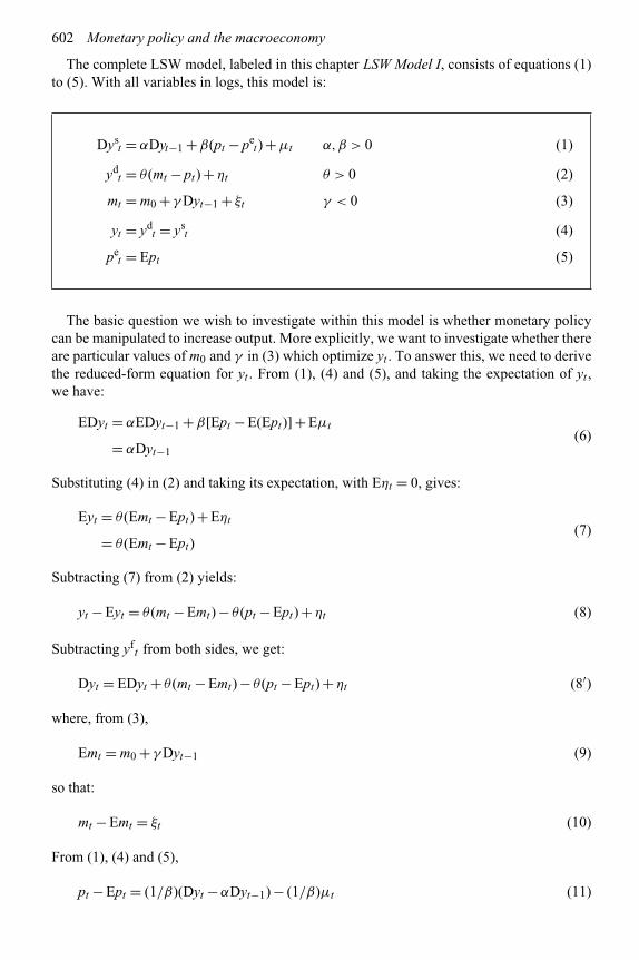
602 Monetary policy and the macroeconomy
The complete LSW model, labeled in this chapter LSW Model I, consists of equations (1)to (5). With all variables in logs, this model is:
Dyst = αDyt−1 +β(pt − pe
t) +μt α,β > 0 (1)
ydt = θ (mt − pt) +ηt θ > 0 (2)
mt = m0 + γ Dyt−1 + ξt γ < 0 (3)
yt = ydt = ys
t (4)
pet = Ept (5)
The basic question we wish to investigate within this model is whether monetary policycan be manipulated to increase output. More explicitly, we want to investigate whether thereare particular values of m0 and γ in (3) which optimize yt . To answer this, we need to derivethe reduced-form equation for yt . From (1), (4) and (5), and taking the expectation of yt ,we have:
EDyt = αEDyt−1 +β[Ept − E(Ept)]+ Eμt
= αDyt−1
(6)
Substituting (4) in (2) and taking its expectation, with Eηt = 0, gives:
Eyt = θ (Emt − Ept) + Eηt
= θ (Emt − Ept)(7)
Subtracting (7) from (2) yields:
yt − Eyt = θ (mt − Emt) − θ (pt − Ept) +ηt (8)
Subtracting yft from both sides, we get:
Dyt = EDyt + θ (mt − Emt) − θ (pt − Ept) +ηt (8′)
where, from (3),
Emt = m0 + γ Dyt−1 (9)
so that:
mt − Emt = ξt (10)
From (1), (4) and (5),
pt − Ept = (1/β)(Dyt −αDyt−1) − (1/β)μt (11)
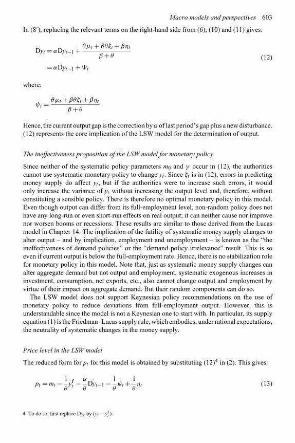
Macro models and perspectives 603
In (8′), replacing the relevant terms on the right-hand side from (6), (10) and (11) gives:
Dyt = αDyt−1 + θμt +βθξt +βηt
β + θ
= αDyt−1 +�t
(12)
where:
ψt = θμt +βθξt +βηt
β + θ
Hence, the current output gap is the correction by α of last period’s gap plus a new disturbance.(12) represents the core implication of the LSW model for the determination of output.
The ineffectiveness proposition of the LSW model for monetary policy
Since neither of the systematic policy parameters m0 and γ occur in (12), the authoritiescannot use systematic monetary policy to change yt . Since ξt is in (12), errors in predictingmoney supply do affect yt , but if the authorities were to increase such errors, it wouldonly increase the variance of yt without increasing the output level and, therefore, withoutconstituting a sensible policy. There is therefore no optimal monetary policy in this model.Even though output can differ from its full-employment level, non-random policy does nothave any long-run or even short-run effects on real output; it can neither cause nor improvenor worsen booms or recessions. These results are similar to those derived from the Lucasmodel in Chapter 14. The implication of the futility of systematic money supply changes toalter output – and by implication, employment and unemployment – is known as the “theineffectiveness of demand policies” or the “demand policy irrelevance” result. This is soeven if current output is below the full-employment rate. Hence, there is no stabilization rolefor monetary policy in this model. Note that, just as systematic money supply changes canalter aggregate demand but not output and employment, systematic exogenous increases ininvestment, consumption, net exports, etc., also cannot change output and employment byvirtue of their impact on aggregate demand. But their random components can do so.
The LSW model does not support Keynesian policy recommendations on the use ofmonetary policy to reduce deviations from full-employment output. However, this isunderstandable since the model is not a Keynesian one to start with. In particular, its supplyequation (1) is the Friedman–Lucas supply rule, which embodies, under rational expectations,the neutrality of systematic changes in the money supply.
Price level in the LSW model
The reduced form for pt for this model is obtained by substituting (12)4 in (2). This gives:
pt = mt − 1
θyf
t − α
θDyt−1 − 1
θψt + 1
θηt (13)
4 To do so, first replace Dyt by (yt − yft ).

604 Monetary policy and the macroeconomy
Equation (13) implies that ∂pt/∂mt = 1. Hence, since both p and m are in logs, prices riseproportionately with the overall increase in the nominal money supply, whether it is due tothe systematic factors γ and m0 or the random component ξt .
To find pet , since pe
t = E(pt), taking the rational expectation of (13) implies that:
pet = E(mt) − (1/θ )yf
t − (α/θ )Dyt−1 (14)
From (14) and (9),
pet = m0 − (1/θ )yf
t +{γ − (α/θ )}Dyt−1 (15)
In (14) and (15), ∂pet/∂Emt = 1, so that the expected price level rises proportionately in the
same period with the systematic component of the nominal money supply, and responds tothe policy parameters γ and m0, but not to the random part ξt of the money supply. Hence,increases in systematic money supply (and systematic demand) proportionately change boththe price level and the expected price level but do not cause a change in output, whereasrandom changes in the money supply change the price level and output but not the expectedprice level.
Diagrammatic analysis of output and price level in the LSW model
The effect of a systematic monetary increase in the LSW model is shown in Figure 17.1. From(2), the aggregate demand curve AD has a negative slope and shifts to the right from AD0 toAD1 with a monetary expansion. From (1), the (short-run) aggregate supply curve SAS hasa positive slope and shifts to the left from SAS0 to SAS1 with an increase in the expectedprice level. Since the latter, from (14), increases proportionately with a systematic monetaryexpansion, such a monetary expansion results in proportionate shifts of both curves, and theeconomy goes directly from point a to point c without an intermediate increase in output.However, a random increase in the money supply cannot be anticipated, so that the expectedprice level does not increase as a result and the supply curve does not shift from SAS. Butthe demand curve does go from AD0 to AD1, with the new equilibrium at point b causing anincrease in both prices and output. Hence, while the systematic increases in money supplydo not bring about an increase in output, unexpected changes in it do so.5
y
P
AD0
AD1
SAS0
y0
P0
P1
SAS1
b
a
c
Figure 17.1
5 If we continue the story further, the unexpected increase in the current price level will have become anticipatedin the following period, so that, barring new sources of shifts in aggregate demand and supply, the economy will

Macro models and perspectives 605
17.2 A compact (Model II) form of the LSW model
Since the price level is a function of the money supply and the expected price level is afunction of the expected money supply, the above model with rational expectations is oftenreplaced by the following more compact one, labeled by us as the LSW Model II.
Lucas supply rule:
Dyt = αDyt−1 +β(mt − met) +μt α,β > 0 (16)
Money supply rule:
mt = m0 + γ Dyt−1 + ξt γ < 0 (17)
Rational expectations:
met = Emt (18)
Note that the assumption of equilibrium in the commodity market has already beenincorporated in (16). From (17) and (18),
mt − met = ξt (19)
Hence, from (16) and (19),
Dyt = αDyt−1 +βξt +μt (20)
where Dyt is again independent of the systematic monetary policy parameters m0 andγ , so thatchanges in these parameters will not change yt . Hence, the policy invariance result also holdsin this model. Note that this is a strong and seemingly surprising result: monetary policy cannotcorrect for the output gap that arises because of persistence in the model. Even if yt < yf
t ,an expansionary systematic monetary policy cannot reduce the output gap, nor increase it.Further, the sources of the output gap are persistence, random disturbances and fluctuationsin the full-employment output, with actual output lagging behind the full-employment level.These provide the basis for the real business cycle (RBC) theories. Given that 0 < α < 1, thedeviations of output from its full-employment level are self-correcting over time.
For another – though misleading – pattern of derivation in the above model, we havefrom (17):
Emt = m0 + γ Dyt−1 (21)
be at point c after the current period. Therefore, the increase in output is likely to be short lived. Its duration willdepend upon the time it takes the public to correct for erroneous price expectations.

606 Monetary policy and the macroeconomy
so that, from (16), (18) and (21):
Dyt = αDyt−1 +βmt −β(m0 + γ Dyt−1) +μt
= (α −βγ )Dyt−1 −βm0 +βmt +μt
(22)
In (22), Dyt depends upon the policy parameters m0 and γ , so that we get the impression thatoutput will depend upon systematic monetary change. However, this would be erroneous sincesubstituting (17) in (22) to eliminate mt again gives (20), which establishes the systematicpolicy irrelevance result.
17.3 The Lucas critique of estimated equations as a policy tool
Suppose the economic researcher were to use (20) to set up an estimating equation of the form:
yt = a0 + a1�Yt + ξt a1 ≥ 0 (23)
where y is output, Y is nominal aggregate demand and ξ is white noise, and found theestimated value of a1 to be positive (i.e. â1 > 0). As argued above, if the policy makerincreased aggregate demand by more than was experienced during the estimation period,a1 would shift, so that â1 would no longer be the relevant magnitude under the reviseddemand policy. Hence, a maintained shift in the expansion of demand does not leave theestimated parameters constant. This is known as the Lucas critique of estimated functions ofthe Lucas–Phillips curve type; if the underlying model of the economy is as set out by Lucas,the parameters of functions such as (23) are not invariant with respect to policy shifts.
Lucas (1973) estimated a variant of (23) for a cross section of countries and found thatcountries with low rates of inflation (such as the USA in the 1950s and 1960s) showedevidence of a positive relationship between output and demand increases while those withhyper-inflation (such as Argentina in the 1950s and 1960s) did not. He thereby concludedthat this relationship shifts as inflation increases, and that the Phillips curve tradeoff does nothold at high and persistent rates of inflation.
Similarly, an estimating equation with unemployment u as the dependent variable would be:
ut = b0 + b1�Yt + ξt b1 ≤ 0 (24)
Note that an estimated function such as (24) does not distinguish between the expectations-augmented Phillips curve, based on errors in price level expectations in labor markets, andthe Lucas supply rule, based on errors in relative commodity prices, so that the estimatedcoefficients would reflect the influence of both types of errors. Equations such as (23) withoutput as the dependent variable or (24) with unemployment as the dependent variable havebeen estimated for a variety of countries and for a variety of time periods. Lucas’s conclusion,that such functions are often unstable under demand policy shifts, is now well established.6
6 Another aspect of the preceding discussion and of the Lucas critique is that economic agents learn from experience,so that their expectations shift if policy shifts. This brings us back to the question of the expectations hypothesesand the role of learning in them. A number of learning mechanisms have been proposed and the speed at whichexpectational errors are eliminated is derived for them. However, they go beyond the concerns of this book andare not examined herein.

Macro models and perspectives 607
However, another of Lucas’s conclusions was that systematic demand increases do not changereal output and unemployment. This has not always been supported in empirical studies, asthe stylized facts on money and output at the beginning of Chapter 14 show.
The Lucas critique in the LSW model
To check on the applicability of the Lucas critique in the LSW model comprising equations(16) to (18), restate (22) compactly as:
yt = a0 + a1yt−1 + a2mt +μt (25)
where a0 = yft − (α − βγ )yf
t−1 − βm0, a1 = (α − βγ ) and a2 = β. If (25) is estimated, itwould yield the estimated values of a1 and a2 as â1 and â2. If â2 > 0, it would be tempting toconclude that the authorities could increase the money supply to increase output. However,as we have shown earlier in Section 17.2, this would not be a valid conclusion. A policychange in the money supply rule would mean a shift in the values of m0 or/and γ . But, asthese shift, a1 and a2 in (25) would shift, as can be seen from a glance at (22), of which (25)is only the compact form. Hence, it cannot be assumed that a1 and a2 are invariant to a policychange. The Lucas critique therefore applies to (25), so that this equation cannot be used as atradeoff for policy formulation. Further, (25) cannot be used for regression estimates acrosspolicy regimes since such estimation assumes constant parameters.7
17.4 Testing the effectiveness of monetary policy: estimates based onthe Lucas and Friedman supply models
The Friedman–Lucas supply function can be stated with output, employment, unemploymentor another real variable, such as the real rate of interest as the dependent variable, and with theexpectational errors in absolute prices, in aggregate demand or with just money supply as theindependent variable. From a monetary policy perspective, the form of the Friedman–Lucassupply function that is usually tested is:
yt = a0 + a1(Mt − M et) +�ja
′jzjt +μt a1 > 0 (26)
where:M = nominal money supplyM e = expected nominal money supplyzj = other exogenous variablesμ = random term.
Equation (26) focuses on money supply as the sole policy variable determining aggregatedemand. Under rational expectations,
M et = EMt (27)
7 For consistent and unbiased estimates using data from a given policy regime – i.e. with constant true values of m0
and γ− estimate (21) and (25). Since there are five reduced form coefficients (a0, a1, a2, m0 and γ ) in equations(24) and (26), while there are only four structural ones (m0, γ , α, β) in (16) to (18), cross-equation restrictionsimplied by (25) will have to be imposed and a simultaneous estimation procedure used.

608 Monetary policy and the macroeconomy
where EMt is proxied by its estimated value EMt = Mt . Similarly, if needed, the estimatedforms of the other variables in (26) can be used to modify this equation, but are omitted here.Therefore, the estimated form of (26) becomes:
yt = a0 + a1(Mt − Mt) +�ja′jzjt +μt a1 > 0 (28)
Equation (28) is a commonly used form of the modern classical output hypothesis for theshort run. In the long run, M = M , so that money supply changes cannot affect y.
17.4.1 A procedure for segmenting the money supply changes into theiranticipated and unanticipated components
To estimate (28), we need the value of M et . Its value is usually the one specified by the
REH and is a function of the information available to the economic agent. Assuming thatthe central bank controls the national money supply, the relevant knowledge would be thatof the public on central bank behavior and on the policy rule that the central bank follows.Assume that this is a rule that gives the money supply function as:
Mt = �iαixit (29)
where xt is a set of exogenous and predetermined variables. Adding in a disturbance term η
gives the money supply rule function:
Mt = �iαixit +ηt (30)
Under the REH, the public is assumed to know the policy function (29) and use the estimatedvalues αi from (30) to calculate the estimated value Mt , where Mt is the rational expectations’proxy for the anticipated money supply, so that:
ηt = Mt − Mt (31)
ηt is the proxy, under the rational expectations hypothesis, for the unanticipated moneysupply.
The nested form of the Lucas model
The nested form of (28) and (26), incorporating both ηt and M , specifies the linear (orlog-linear) estimating equation as:
yt = β0 +β1Mt +β2ηt +�jγjzjt +μt (32)
If β1 = 0, the anticipated values of money supply do not affect real output, so that this finding
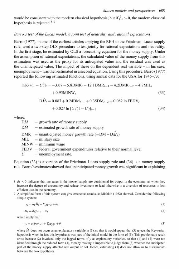
Macro models and perspectives 609
would be consistent with the modern classical hypothesis; but if β1 > 0, the modern classicalhypothesis is rejected.8,9
Barro’s test of the Lucas model: a joint test of neutrality and rational expectations
Barro (1977), in one of the earliest articles applying the REH to the Friedman–Lucas supplyrule, used a two-step OLS procedure to test jointly for rational expectations and neutrality.In the first stage, he estimated by OLS a forecasting equation for the money supply. Underthe assumption of rational expectations, the calculated value of the money supply from thisestimation was used as the proxy for its anticipated value and the residual was used asthe unanticipated value. The impact of these on the dependent real variable – in his case,unemployment – was then estimated in a second equation. Using this procedure, Barro (1977)reported the following estimated functions, using annual data for the USA for 1946–73:
ln[U/(1 − U )]t = −3.07 − 5.8DMRt − 12.1DMRt−1 − 4.2DMRt−2 − 4.7MILt
+ 0.95MINWt (33)
DMt = 0.087 + 0.24DMt−1 + 0.35DMt−2 + 0.082 ln FEDVt
+ 0.027 ln [U/(1 − U )]t−1 (34)
where:DM = growth rate of money supplyDM = estimated growth rate of money supply
DMR = unanticipated money growth rate (=DM−D∧Mt)
MIL = military sizeMINW = minimum wageFEDV = federal government expenditures relative to their normal levelU = unemployment rate.
Equation (33) is a version of the Friedman–Lucas supply rule and (34) is a money supplyrule. Barro’s estimates showed that unanticipated money growth was significant in explaining
8 β1 < 0 indicates that increases in the money supply are detrimental for output in the economy, as when theyincrease the degree of uncertainty and reduce investment or lead otherwise to a diversion of resources to lessefficient uses in the economy.
9 A simplified form of this system can give erroneous results, as Mishkin (1982) showed. Consider the followingsimple system:
yt = a1Mt +�jgjzjt + θt (1)
Mt = b1yt−1 +�t (2)
which imply that:
yt = a1b1yt−1 +�jgjzjt + θt (3)
where Mt does not occur as an explanatory variable in (3), so that it would appear that (3) rejects the Keynesianhypothesis when in fact this hypothesis was part of the initial model in the form of (1). This problematic resultarose because (2) involved only the lagged terms of y as explanatory variables, so that (1) and (2) were notidentified through the reduced form (3), thereby making it impossible to judge from (3) whether the anticipatedpart of the money supply affected real output or not. Hence, estimating (3) does not allow us to discriminatebetween the two hypotheses.
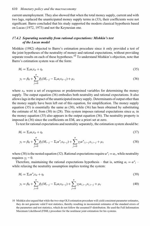
610 Monetary policy and the macroeconomy
current unemployment. They also showed that when the total money supply, current and withtwo lags, replaced the unanticipated money supply terms in (33), their coefficients were notsignificant. Barro concluded that his study supported the modern classical hypothesis basedon Lucas (1972, 1973) and not the Keynesian one.
17.4.2 Separating neutrality from rational expectations: Mishkin’s testof the Lucas model
Mishkin (1982) objected to Barro’s estimation procedure since it only provided a test ofthe joint hypotheses of the neutrality of money and rational expectations, without providingseparate results on each of these hypotheses.10 To understand Mishkin’s objection, note thatBarro’s estimation system was of the form:
Mt = �iαixit +ηt (35)
yt = β0 +n∑
j=0
βj(Mt−j −�iαixit−j) +μt (36)
where xit were a set of exogenous or predetermined variables for determining the moneysupply. The output equation (36) embodies both neutrality and rational expectations. It alsoallows lags in the impact of the unanticipated money supply. Determinants of output other thanthe money supply have been left out of this equation, for simplification. The money supplyequation (35) is essentially the same as (30), while (36) has been obtained by substitutingthe estimate of Mt from (30) in (28). This system imposes rational expectations since αi inthe money equation (35) also appears in the output equation (36). The neutrality property isimposed in (36) since the coefficients on EMt are a priori set at zero.
To test for rational expectations and neutrality separately, the estimation system should be:
Mt = �iαixit +ηt (37)
yt = β0 +n∑
j=0
βj(Mt−j −�iα∗ixit−j) +
n∑j=0
γjα∗i,t−jxi,t−j +μt (38)
where (38) is the nested equation (32). Rational expectations require α∗i =αi, while neutrality
requires γj = 0.Therefore, maintaining the rational expectations hypothesis – that is, setting αi = α∗
i –while relaxing the neutrality assumption implies testing the system:
Mt = �iα∗ixit +ηt (39)
yt = β0 +n∑
j=0
βj(Mt−j −�iαixit−j) +n∑
j=0
γjαi,t−jxi,t−j +μt (40)
10 Mishkin also argued that while the two-step OLS estimation procedure will yield consistent parameter estimates,they do not generate valid F-test statistics, thereby resulting in inconsistent estimates of the standard errors ofthe parameters and test statistics, which do not follow the assumed F-distribution. He used the Full InformationMaximum Likelihood (FIML) procedure for the nonlinear joint estimation for his systems.
Macro models and perspectives 611
The null hypothesis of neutrality – that is, γj = 0 – can be tested by comparing the estimates ofthe system (39) and (40) with those from (35) and (36). Maintaining the neutrality hypothesiswhile testing for rational expectations requires estimating:
Mt = �iαixit +ηt (41)
yt = β0 +n∑
j=0
βj(Mt−j −�iα∗ixit−j) +μt (42)
The null hypothesis of α∗i = αi is tested by comparing the estimates from (41) and (42)
against those from (35) and (36).Mishkin’s tests for the USA on quarterly data for 1954–76 used unemployment and output
as the dependent variables, and nominal GNP and the rate of inflation among the independentvariables. He reported that while the REH was not rejected by the data, neutrality was. Further,the estimated coefficients of the anticipated and unanticipated demand variables were verysimilar in magnitude. Therefore, Mishkin’s results supported the Keynesian hypothesis andrejected the modern classical one on the key issue of the neutrality of anticipated aggregatedemand and of demand management policies. These results did not reject the REH, which ismerely a procedure for modeling expectations and, as noted earlier, is not a priori inconsistentwith either the Keynesian or the modern classical theories.
Among several other studies, Frydman and Rappoport (1987) also tested for the distinctionbetween the impact of anticipated and unanticipated monetary policy by examining the impactof the growth rate of money on output. Their findings reject this distinction for the short-run determination of output, with this rejection robust to different specifications of rationalexpectations and of the employment level of output.
We conclude that there is by now very substantial evidence that this distinction is notvalid and, further, that anticipated monetary policy is not neutral, at least for the short run.These findings are not surprising in view of the stylized facts listed at the start of Chapter 14.Therefore, models of the Lucas and the Sargent and Wallace variety do not provide a usefulbasis for macroeconomic analysis and policy.
17.5 Distinguishing between the impact of positive and negativemoney supply shocks
It is sometimes argued that decreases in the money supply are likely to have a stronger impactthan increases in it. There can be several reasons for this. Among these are:
1. A decrease in the money supply represents a decrease in credit in the economy, so thatborrowers are forced to curtail their economic activities, and this reduces output in theeconomy. By comparison, an increase in the money supply means a greater willingnessby the financial intermediaries to lend, which does not result in the same urgency toborrow as a decrease in loans to repay.11
2. Contractionary policies are likely to be pursued during booms with full employment anda high demand for investment and additional borrowing, whereas expansionary policiesare likely to be pursued during recessions when firms generally face inadequate demand
11 An analogy sometimes used is that one can pull on a string but not push on it.

612 Monetary policy and the macroeconomy
for their products, often have excess capacity and do not have enough incentive toincrease their investment and borrowing. That is, the impact of the two types of policiesalso depends on the phase of the business cycle with which the two are associated.
3. The economy is likely to possess some downward rigidity in prices and nominal wageswhereas it possesses a higher degree of flexibility for increases in them. Decreases in themoney supply run into this downward rigidity and are more likely to have real effects,while most or all of the impact of increases in the money supply could be only on pricesand the nominal but not the real value of output.
The Barro and Mishkin tests can be modified to test for this differential impact. We illustratethis by modifying the Friedman–Lucas supply function to:
yt = a0 + a+1M u
t +�ja′jzjt +μt (43)
and its nested form (32) to:
yt = a0 + a+1M u+
t + a−1M u−
t +β+1M e+
t +β−1M e−
t +�jαjzjt +μt (44)
where:M u+ = unanticipated increase in the money supplyM u− = unanticipated decrease in the money supplyM e+ = expected (anticipated) increase in the money supplyM e− = expected (anticipated) decrease in the money supply
and zj are the other variables in the determination of output. The other aspects of theestimation procedures of Barro and Mishkin remain as specified earlier. In particular,the actual estimation should allow for lags and other independent variables. The Mishkin(1982) procedure specified above can be suitably modified to check on neutrality, rationalexpectations and asymmetrical effects.
Some empirical studies do report evidence of the asymmetrical effects – and non-neutrality – of monetary policy. Our earlier arguments suggest the possibility that negativeshocks to money have greater impact than positive ones. For example, Cover (1992), usingMishkin’s (1982) procedure, finds for US quarterly data that positive shocks to M1 had noeffect on output, whereas negative ones did so. Ratti and Chu (1997) confirm for Japan theasymmetry between the effects of positive and negative shocks. They further report thatunanticipated changes in a wide definition of money did not have a significant impact onoutput in Japan.
17.6 LSW model with a Taylor rule for the interest rate
As Chapter 13 pointed out, in recent decades many central banks have chosen to set the interestrate rather than the money supply. Assume that the central bank uses a contemporaneousTaylor rule with price level targeting12 of the form:
rTt = r0 +λy(yt − yf ) +λP(Pt − PT) λy,λP > 0 (45)
There are two ways of integrating this rule in the LSW framework. One is to use the moneydemand function to derive the endogenous money supply that keeps the financial markets in
12 This has been done to avoid having the price level in some equations and the inflation rate in others within ourmodel. P is the log of the price level and T indicates its target value.

Macro models and perspectives 613
equilibrium (see Chapter 13) and then use the resulting money supply function in the rest ofthe LSW model. The other method is to replace the money supply function in the originalLSW model by the Taylor rule and make appropriate changes in the aggregate demandequation. The following derivations are based on the second method.
For the linear forms of the various functions, the IS equation for the open economy derivedin Chapter 13 was:
yd = α[{c0 − cyt0 + i0 − irr + g + xc0 − xcρρr}+ (1/ρr).{− zc0 + zcyt0 − zcρρr}] (46)
where:
α =(
1
1 − cy + cyty + 1ρr zcy(1 − ty)
)> 0
and ρr =ρP/PF. The definitions of the symbols are as given in Chapter 13. For simplification,assume the general form of the IS equation to be:
ytd = y0 − θ1rT − θ2Pt (47)
The resulting LSW model with the stochastic forms of the preceding IS equation and theTaylor rule and all variables in logs is:
Dyst = αDyt−1 +β(Pt − Pe
t) +μt α,β > 0 (48)
ydt = θ0 − θ1rt − θ2Pt + νt θ1,θ2 > 0 (49)
rt = rTt +η1t (50)
rTt = r0 +λyDyt +λP(Pt − PT) +η2t λy,λP > 0 (51)
yt = ydt = ys
t (52)
Pet = EPt (53)
where Dy = yt − yf , μ is supply shocks, ν is IS shocks, η2 is the monetary policy shock andη1 is the stochastic slippage in the control of the economy’s interest rate by the central bank.All disturbances are taken to be white noise.
Taking the rational expectation of the aggregate supply equation (48), we have:
EDyst = αEDyt−1 +β[EPt − E(EPt)]+ Eμt
= αDyt−1
(54)
so that:
Dyst − EDys
t = β(Pt − EPt) +μt (55)
614 Monetary policy and the macroeconomy
Further, from (48) and (53):
Pt − EPt = (1/β)(Dyt −αDyt−1) − (1/β)μt (56)
Now, taking the rational expectation of the IS equation (49), we have:
Eydt = θ0 − θ1Ert − θ2EPt (57)
Subtracting (57) from (49) yields:
ydt − Eyd
t = −θ1(rt − Ert) − θ2(Pt − EPt) + νt (58)
where rt is given by:
rt = r0 +λyDyt +λP(Pt − PT) +η2t +η1t (59)
so that:
Ert = r0 +λyEDyt +λP(EPt − PT) (60)
Hence:
rt − Ert = λy(Dyt − EDyt) +λP(Pt − Ept) +η2t +η1t (61)
Substituting (61) in (58) and imposing equilibrium, so that yt = ydt = ys
t , and Dyt = Dydt =
Dyst , we have:
yt − Eyt = −θ1{λy(Dyt − EDyt) +λP(Pt − EPt) +ηt}− θ2(Pt − EPt) + νt (62)
where ηt = η1t +η2t . Since yt − Eyt = Dyt − EDyt , where Dy = y − yf , (62) becomes:
Dyt = EDyt − θ1λyDyt + θ1λyEDyt − θ1λP(Pt − EPt) − θ1ηt − θ2(Pt − EPt) + νt (63)
(1 + θ1λy)Dyt = (1 + θ1λy)EDyt − (θ1λP + θ2)(Pt − EPt) − θ1ηt + νt
= [{(1 + θ1λy)αDyt−1 − (1/β)(θ1λP + θ2){(Dyt −αDyt−1) −μt}− θ1ηt + νt
{(1 + θ1λy) + (1/β)(θ1λP + θ2)}Dyt
= {(1 + θ1λy) + (1/β)(θ1λP + θ2)}αDyt−1 −{(1/β)(θ1λP + θ2)}μt − θ1ηt + νt (64)
Replacing {(1 + θ1λy) + (1/β)(θ1λP + θ2)} by a1 and {(1/β)(θ1λP + θ2)} by a2, we get:
Dyt = αDyt−1 − (a2/a1)μt − (1/a1)θ1ηt + (1/a1)νt (65)
where α is the fraction by which the economy, on its own, adjusts the current period’s outputgap as a fraction of last period’s gap. It is independent of the systematic policy parametersλy, λP embodied in the Taylor rule. However, random IS shocks (μ), monetary sector shocks(η1) and policy shocks (η2) do impact on the output gap, with this impact a function of variousparameters, including those of policy. This conclusion is similar to that derived earlier from

Macro models and perspectives 615
the LSW model with a money supply function. In particular, systematic policy parameters donot affect output in both models. This is especially surprising in the current model with theTaylor rule, which explicitly targets the output gap. This finding highlights the point that, inthis model, the driving conclusions on output are given by the nature of the supply rule andthe expectations hypothesis, not by the monetary policy rule, which determines systematicmonetary policy. In the LSW model, this supply rule is the Lucas rule. Replacing it by aKeynesian or NK supply function is essential for showing the effectiveness of systematicpolicies in changing the output gap.
Note that the policy parameters do affect the impact on output of each of the disturbances.
17.7 Testing the effectiveness of monetary policy: estimates fromKeynesian models
17.7.1 Using the LSW model with a Keynesian supply equation
A Keynesian supply function would differ from the Lucas one in several ways. One, it wouldallow both anticipated and unanticipated money supply changes to affect output. Two, asargued in Chapter 15, the effect of money supply changes on output would depend on thestate of the economy and the degree of involuntary unemployment. Three, in Keynesianmodels, the impact of money supply changes on output can occur without a prior change inthe price level, so that the LSW(II) model with the money supply as an explanatory variableis preferable to the LSW model with the price level. Further, note that, in the Keynesiancontext, the dependence of yt on yt−1 occurs because Keynesian models allow for staggeredwage contracts longer than one period as well as the gradual adjustment of output to shocks.
Adapting the Friedman–Lucas supply function to a Keynesian format by replacing theunanticipated money supply (mt – me
t) by the total money supply mt gives:
Dyt = αyt−1 +βtmt +μt α,β > 0 (66)13
where the definitions of the symbols are as given earlier. As a reminder, note that the lower-case letters are logs of variables and Dy is the deviation from the full-employment leveland not a change from the previous period’s level. For Keynesian models, since the moneymultiplier depends on the state of the economy, the value of βt should be a function of theoutput gap.
If we specify the complete model as consisting of the money supply function (17) and theKeynesian output supply function (66), we find that:
Dyt = (α +βtγ )Dyt−1 +βtm0 +μt +βtξt (67)
where Dyt depends upon the policy parameters m0 and γ , which can be used to achieve thedesired objectives with respect to yt , and upon the money multiplier βt , as well as on theprevious period’s deviation from full-employment output.
Equation (67) is not an appealing format for the Keynesian supply function. A better formatseems to be one where the deviation of output from its full-employment level depends not
13 β in true Keynesian models would properly not be a constant but would be a function of the deviation of outputfrom full-employment level. However, Sargent and Wallace (1976) proposed Dyt = αDyt−1 +βmt +μt as theKeynesian reduced-form equation, with a constant β, and it is frequently cited as such.
616 Monetary policy and the macroeconomy
on the money supply but on its change. The output supply function consistent with thisidea is:
Dyt = αDyt−1 +βt(mt − mt−1) +μt, α,β > 0 (68)
The LSW money supply rule (17) can also be reformulated as:
mt − mt−1 = γ1(yt−1 − yt−2) − γ2(yft−1 − yf
t−2) + (ξt − ξt−1) γ1,γ2 < 0 (69)
This modification of the LSW money supply rule allows for differential response of themoney supply to changes in actual output versus changes in full-employment output. Sinceγ1, γ2 < 0, the monetary authority decreases the money supply if the actual output rose lastperiod and increases it if there was a rise in the full-employment output.
Equations (68) and (69) yield:
Dyt = αDyt−1 +βtγ1(yt−1 − yt−2) −βtγ2(yft−1 − yf
t−2) +μt +βt(ξt − ξt−1) (70)
which implies that the monetary authority can change its policy parameters γ1, γ2 to affectoutput deviations from full employment. Therefore, policy irrelevance does not occur in thisKeynesian model, irrespective of any assumption on the rationality of expectations. However,the Lucas critique will still apply since the coefficient of yt−1 in (70) depends on the monetarypolicy parameters γ1 and γ2, which will change with a policy shift.
17.7.2 Gali’s version of the Keynesian model with an exogenous money supply
Chapter 15 reported the findings from Mishkin’s (1982) test from reduced-form equationsthat money was not neutral while rational expectations were valid.
Gali (1992) uses a structural model that is Keynesian with a Phillips curve. His model, inlogs, is:
IS equation:
yt = μst +α −σ (Rt − E�pt−1) +μIS
t (71)
LM equation:
mt − pt = φyt −λRt +μmdt (72)
Money supply process:
�mt = μmst (73)
Phillips curve:
�pt = �pt−1 +β(yt −μst) (74)
where the symbols designate the logs of the relevant variables, except for R (which standsfor the level of the nominal interest rate). μs, μIS, μmd and μms are the stochastic processesfor output supply, expenditures, money demand and money supply respectively. The IS andLM equations are consistent with the Lucas model, except that they provide greater detail.

Macro models and perspectives 617
The major difference between this Keynesian model and the LSW models lies in thespecification of output supply. Gali specifies it by the Phillips curve, so that changes inthe inflation rate between periods determine the variations μs in output from its equilibriumlevel, whereas the LSW model uses relative price misperceptions to explain such deviations.In the Gali model, output can change due to supply shocks through μs, or demand shocks dueto μIS, μmd or μms. Positive demand shocks increase both output and prices while positivesupply shocks increase output and decrease prices. Monetary shocks are transmitted to thereal sector only through changes in the interest rate.
The segregation of the experienced shocks into four different types requires specialassumptions on their origin or impact. Gali separated the supply shocks from the demandshocks by the assumption that the former have long-run effects on output while the latter donot. The IS shocks were separated from the money market shocks by the assumption thatthe latter do not have contemporaneous impact on aggregate demand in the same quarter,since their impact occurs through the changes in interest rates impinging on investment. Themoney demand and supply shocks were separated under three alternative assumptions, whichwe do not report here.
Gali’s data was quarterly for the USA for 1955:I to 1987:IV. The monetary aggregateused was M1 and the interest rate was represented by the three-month Treasury bill rate.The findings supported the Keynesian claim that demand shocks do cause output changeswhile rejecting its claim that they, rather than supply shocks, were the dominant source ofoutput fluctuations. Supply shocks had a substantial deflationary impact and accounted forabout 70 percent of output variability over the business cycle. However, their impact on thenominal interest rate was small.
Increases in M1 increased output, reaching a peak in about four quarters, accompanied byincreases in inflation and nominal interest rates but decreases in the real rate. While the moneysupply shocks accounted for most of the short-run variability of the nominal and real interestrates and for some variability in output over the business cycle, there was no long-run effecton output or the real rate, though this result really emanates from the built-in assumptions,but only on the inflation rate. Money demand shifts had a much faster impact on prices thanmoney supply shifts and significant impact on real balances, but little influence on outputvariability or the real rate.
The impact of the IS shocks on output started within the same quarter as the shock, clearlyjust a result of the assumptions made, reached a peak two quarters after the shock but almostvanished after four quarters. However, such shocks had permanent effects on money growth,inflation and the nominal rate. While they increased the nominal rate, they first increasedthe real rate but, because of their impact on inflation, soon led to a decline in the real rate,which returned to its initial level about two years after the shock. IS shocks accounted for asubstantial part of the business fluctuations.
Gali’s findings, therefore, support the Keynesian conclusions that demand shocks do causevariations in output. Further, money supply variations had a longer-lasting impact on outputthan IS shocks. However, the major source of the variations in output was supply ratherthan demand shocks. Demand shocks did not produce long-run effects on output and the realrate of interest.14 While Gali’s model did not distinguish between positive and negative
14 Note that these findings are affected by the assumptions made to segment the shocks to the economy, so thatany errors in these assumptions could lead to erroneous results. For example, if aggregate demand changes docause long-run changes in output, such impact would have been erroneously attributed to supply factors.
618 Monetary policy and the macroeconomy
money supply shocks or test for asymmetry in their effects, it can clearly be modifiedto do so.
In another study, for a large number of countries, Bullard and Keating (1995) used vectorautoregression to investigate the impact of inflation on output. In their procedure, theyidentified the permanent component of inflation as being due to permanent changes in themoney growth rate while exogenous shocks to output were taken to cause only transitoryshocks to inflation. Their finding was that permanent shocks to inflation did not permanentlyincrease the level of output for most of the countries but did do so for certain low-inflationcountries. In general, the estimated effects were positive for low-inflation countries, andlow or negative for high inflation countries. Money is not neutral under these findings. Thispattern of the effects of inflation on output seems to reflect the opinion of most monetaryeconomists.
17.8 A compact form of the closed-economy new Keynesian model
The following presents a compact model of the new Keynesian model along the linesdiscussed in Chapter 15 (Bernanke and Woodford, 1997; Clarida et al. (Clarida, Gali andGertler, CGG), 1999; Levin et al. 1999, 2001). It has three core equations: the IS equation,the output supply equation and the monetary policy rule.
IS equation:
xt = Et(xt+1) −ψ(Rt − Eπt+1) + gt (75)
where x = y − yf , r is real interest rate while R is the nominal rate, π is the inflation rateand g represents all sources of expenditure (e.g. government deficits) other than investment.Optimizing forward-looking consumers and firms, the Fisher equation for perfect capitalmarkets (so that rt = Rt − Eπt+1) and rational expectations have been incorporated in thisderivation of the IS equation.
Price adjustment process (“new Keynesian Phillips curve”):
πt = αxt +βEtπt+1 + vt (76)
where x is the output gap, acting as a proxy for marginal cost, mc, which rises with anincrease in output. Firms rationally anticipate future inflation and smooth price adjustments.vt = ρvt−1 +ηt and η is a random variable with a zero mean and constant variance. Besidesother sources of disturbances, it can encompass deviations from the linear impact of theoutput gap on marginal cost.15
The preceding price adjustment equation can be rewritten as the output supply equation:
xt = (1/α)πt − (β/α)Etπt+1 − (1/α)vt (77)
In this format, the output gap responds to both current and future inflation.
15 See Gali and Gertler (1999), Clarida et al. (1999, p. 1667, fn 15).
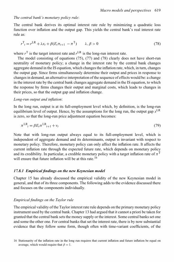
Macro models and perspectives 619
The central bank’s monetary policy rule:
The central bank derives its optimal interest rate rule by minimizing a quadratic lossfunction over inflation and the output gap. This yields the central bank’s real interest raterule as:
rTt = rLR +λxt +β(Etπt+1 −πT) λ,β > 0 (78)
where rT is the target interest rate and rLR is the long-run interest rate.The model consisting of equations (75), (77) and (78) clearly does not have short-run
neutrality of monetary policy; a change in the interest rate by the central bank changesaggregate demand in the IS equation, which changes the inflation rate, which, in turn, changesthe output gap. Since firms simultaneously determine their output and prices in response tochanges in demand, an alternative interpretation of the sequence of effects would be: a changein the interest rate by the central bank changes aggregate demand in the IS equation, to whichthe response by firms changes their output and marginal costs, which leads to changes intheir prices, so that the output gap and inflation change.
Long-run output and inflation:
In the long run, output is at its full-employment level which, by definition, is the long-runequilibrium level of output. Hence, by the assumptions for the long run, the output gap xLR
is zero, so that the long-run price adjustment equation becomes:
πLRt = βEtπ
LRt+1 + vt (79)
Note that with long-run output always equal to its full-employment level, which isindependent of aggregate demand and its determinants, output is invariant with respect tomonetary policy. Therefore, monetary policy can only affect the inflation rate. It affects thecurrent inflation rate through the expected future rate, which depends on monetary policyand its credibility. In particular, a credible monetary policy with a target inflation rate of πT
will ensure that future inflation will be at this rate.16
17.8.1 Empirical findings on the new Keynesian model
Chapter 15 has already discussed the empirical validity of the new Keynesian model ingeneral, and that of its three components. The following adds to the evidence discussed thereand focuses on the components individually.
Empirical findings on the Taylor rule
The empirical validity of the Taylor interest rate rule depends on the primary monetary policyinstrument used by the central bank. Chapter 13 had argued that it cannot a priori be taken forgranted that the central bank sets the money supply or the interest. Some central banks set oneand some the other one. For central banks that set the interest rate, there is by now substantialevidence that they follow some form, though often with time-variant coefficients, of the
16 Stationarity of the inflation rate in the long run requires that current inflation and future inflation be equal onaverage, which would require that β = 1.

620 Monetary policy and the macroeconomy
Taylor rule, even when they do not explicitly announce this as their practice (see Chapter15, Section 15.6). In general, the likelihood of a finding of the Taylor rule is very high forcentral banks that attempt to stabilize aggregate demand and control inflation through interestrates. However, since the coefficients of the Taylor rule depend on central bank preferencesand the economy’s constraints, there will be differences in the estimated coefficients of theTaylor rule among countries and even among different monetary policy regimes (e.g. with adifferent head of the central bank) of any given country.
In any case, central banks do not explicitly disclose their form of the Taylor rule andits coefficients for the output gap and the deviation of inflation from its target level, sothat it needs to be estimated from ex post data. While some form of the Taylor rule doesquite well empirically, its consistency with the new Keynesian models requires a forward-looking version. Levin et al. (1999, 2001) present the estimated coefficients of the Taylorrule from several studies, with the coefficients, and sometimes the rule itself, differing quitesignificantly between the studies. They conclude that a simple version of the inflation andoutput-targeting rule for the US economy performs quite well for the USA, and that a robustpolicy rule includes responses to a short-horizon forecast of inflation, not exceeding one year,and the current output gap. It also incorporates a high degree of policy inertia.
Maria-Dolores and Vazquez (2006) compare the performance of four (contemporaneous,backward-looking, a priori forward-looking, and the forward-looking rule derived from thecentral bank’s optimization of its loss function) types of Taylor rule. They report that the newKeynesian model does much worse with a rule derived from the central bank’s optimizationthan the backward-looking and the simple a priori forward-looking rules. Further, a simpleautoregressive model of the interest rate can sometimes do better than the Taylor rule, asDepalo (2006) reports for Japan.
Empirical findings on the new Keynesian price adjustment equation
Rudd and Whelan (2003) test the general form of the forward-looking NK output equation:
πt = λxt +βEtπt+1 + vt (80)
where x can be specified as the output gap or the deviation of the unemployment rate from thenatural one. They report that this equation performs very poorly for USA data. Empirically,current inflation is negatively, not positively, related to the future output gap; intuitively put,inflation is a negative leading indicator of future output. One reason for such a result couldbe that their proxy used for full-employment output is a poor one. A second reason could bethat, since marginal cost is unobservable, the output gap in the NKPC was used as a proxy forreal marginal cost (i.e. the ratio of marginal cost to price), but may be a poor proxy. Anotherproxy that has been suggested for the real marginal cost is labor’s share in income (Gali andGertler, 1999), but this also has not given much better results.
A third reason for the poor performance of the NKPC could be the high degree of persistencein inflation, which depends heavily on its own lagged values (Rudd and Whelan, 2003; Maria-Dolores and Vazquez, 2006). To capture this persistence, one suggestion is to replace theNKPC by a hybrid rule, say of the form:
πt = δ1
n∑i=1
πt−i +α
∞∑j=0
β jEtxt+j (81)

Macro models and perspectives 621
A simpler form of this equation would use, for the lagged terms, only last period’s inflationrate. However, for the NKPC, the justification for the backward-looking, rather than theforward-looking, inflation term on the right-hand side is problematical: for one thing,interpreting (81) as a form of (80) would be a denial of rational expectations. Further, sincepersistence plays a big part in inflation, the estimate α may not prove to be significant, sothat (81) would reduce to just a form of static expectations. However, even if α proves to besignificant, the estimated contribution of the forward output gaps may prove to be relativelysmall. Moreover, the estimated coefficients of this equation may shift with policy, so that theLucas critique applies to them.
Further, as mentioned in Chapter 15, Mankiw (2001) provides three inconsistenciesbetween this sticky price adjustment equation and the stylized facts about the relationshipbetween inflation and unemployment. Among these inconsistencies are that this process doesnot generate persistence in inflation but does generate implausible dynamic adjustments ininflation and unemployment in response to monetary shocks. This study reports that therelationship that best fits the facts is the backward-looking one:
πt = βπt−1 +α(ut − un) + vt (82)
which is closer to the traditional Phillips curve, or to one with static or adaptive expectations.To provide a theoretical justification consistent with the current intertemporal optimizingapproach in new Keynesian economics, Mankiw and Reis (2002, 2006a,b) replace the stickyprice process by a sticky information one. The latter implies a backward-looking inflationaryprocess which generates persistence in inflation, so that there is a significant differencebetween the sticky price adjustment and the sticky information equations of the Phillips curve.
17.8.2 Ball’s Keynesian small open-economy model with a Taylor rule
Ball (1999, 2000) presents the following compact Keynesian model, with all variables inlogs, for a small open economy:
IS equation:
yt = −βrt−1 + δet−1 +λyt−1 + εt (83)
Phillips curve:
πt = πt−1 +αyt−1 + γ (et−1 − et−2) +ηt (84)
Exchange rate determination:
et = θrt + νt (85)
In these equations, y is the log of output, r is the real interest rate, e is the log of the realexchange rate17 (a higher value of e means appreciation of the domestic currency), π isthe current inflation rate and ε,η and ν are white noise terms. All parameters are taken to
17 For small open economies, the literature indicates that the central bank’s policy function should include theexchange rate in addition to inflation and output among its variables (see, for example, Ball, 1999, 2000), thoughrules excluding the exchange rate also seem to do quite well.

622 Monetary policy and the macroeconomy
be positive. (83) is an open-economy IS equation, with commodity demand depending on the(lagged values of the) real interest rate and the real exchange rate. (84) is an open-economybackward-looking price/inflation adjustment relationship, with the change in the inflationrate a function of lagged output and the lagged change in the exchange rate. The change inthe exchange rate affects inflation through imports since depreciation increases import prices,which increases the domestic price level. (85) has a negative relationship between the interestrate and the exchange rate; an increase in the domestic interest rate increases capital inflowsinto the domestic country, which causes an appreciation of the domestic currency (i.e. theexchange rate rises). This model clearly embodies the short-run non-neutrality of aggregatedemand and therefore of monetary policy, and is consistent with the new Keynesian stickyprice hypothesis.
The preceding model is missing an equation for the money market. Such an equation can bethe LM equation under the assumption of an exogenous money supply or an interest rate policyrule, such as the Taylor rule. Ball assumed that the central bank sets the real interest rate as:
rt = a0rt−1 + aπ [E(πt+4|It) −πt∗]+ ayygapt +μt (86)
where πt∗ = πt − γ et−1; that is, the central bank makes the desired long-run inflation rate
invariant to changes in the exchange rate by filtering out the impact of lagged exchange ratechanges on the current inflation rate.18 y gap is the output gap, defined as the deviation ofoutput from its full-employment level.
17.9 Results of other testing procedures
The findings in numerous empirical studies have ranged back and forth against the neutralityassumption. We do not intend to review many more studies but do consider the findingsof a different type of study to be worth mentioning. As against the use of compact (small)reduced-form models reported above from the works of Barro, Mishkin, Gali, and Bullardand Keating, Mosser (1992) based her findings on four large structural macroeconometricmodels, well established in the late 1980s and 1990s.19 These were used to generate theelasticities of real output, real interest rates and various other real variables with respect tomonetary variables such as M1 and non-borrowed reserves held by banks. The estimatedelasticities were significant not only for the first four quarters but for periods longer than12 quarters for many of the real variables. For real output, the elasticities were positive andcontinued to increase up to 12 quarters, and were significant (either positive or negative)even at 40 quarters. Hence, not only were the monetary variables not neutral, the estimatedlags were very long.
17.10 Summing up the empirical evidence on monetary neutrality andrational expectations
The results reported from Mishkin (1982), Gali (1992), Mosser (1992) and Ball (1999, 2000),as against Barro’s (1977), supported the Keynesian theory and rejected the modern classical
18 To illustrate, for China, Wang and Handa (2007) estimate (83) to (85) by a simultaneous equations techniqueand estimate the Taylor-rule equation (86) using cointegration and error-correction modeling. They find supportfor both this rule and the above model for China, a developing economy.
19 These were: the Bureau of Economic Analysis model, the Data Resources Inc. model, the Federal ReserveBoard/MPS model and the Wharton Econometric Forecasting Associates model.

Macro models and perspectives 623
one on the critical difference between them on the neutrality of anticipated money supplychanges and the continual clearance of all markets. This implies rejection of the Friedman–Lucas supply rule, which incorporates the neutrality of anticipated money supply changes.In general, in spite of its optimizing microeconomic foundations and their intellectualappeal, the modern classical macroeconomic models have not been an unqualified empiricalsuccess.
Another aspect of neutrality modeling worth noting is that the supply functions usedembody either neutrality (for classical models) or non-neutrality (for Keynesian models) ofsystematic monetary policy. However, empirical evidence suggests that systematic monetarypolicy can be neutral sometimes and non-neutral at other times, and that the “degree of non-neutrality” can be variant in intermediate cases, though it is a priori difficult to separate thesecases (Lucas, 1994, 1996). These results need not come as a big surprise; the various theoriespresented in Chapters 14 and 15 indicate that there can be very many different causes of non-neutrality in the economy: staggered wage contracts and the lagged adjustment of nominalwages to prices; disequilibrium factors in the neoclassical model; deficient demand in theKeynesian model; relative price errors in a Lucas-type model; sticky prices in certain markets,sticky information and sticky pensions and other predetermined sources of incomes, etc.Consequently, if our estimating equation allows only the black/white scenario of neutralityversus non-neutrality, when part of the data is from a neutral sample and part is from a non-neutral one, we are likely to get a mixed bag of empirical results, varying with the relativeweights of the two types of data in our sample.
Overall, while there is a somewhat mixed bag of empirical studies favoring one or theother of these hypotheses, the empirical evidence seems more often to favor the short-runnon-neutrality of money rather than its neutrality. The evidence also seems to favor the findingthat there is a difference between the effects of rationally anticipated money supply changesand those of unanticipated price changes, but both can have short-run effects on real output.
By comparison, the empirical evidence on the rationality of expectations does not, ingeneral, reject it. In any case, its assertion that economic agents take account of all availableinformation rather than merely that on the past, seems to be incontrovertible. However,at the level of implementation, whether this hypothesis justifies the interpretation of themodern classical approach that the expected values for the next few quarters or even yearsare the long-run equilibrium ones is highly doubtful. The more realistic interpretation clearlyseems to be the Keynesian one: the rationally expected values are related to the actual futurevalues, which depend on the actual performance of the economy, which is not necessarilythe full-employment one, and the stage of the business cycle.
17.11 Getting away from dogma
The LSW model makes the implicit assumption, derived from perfectly competitive andefficient markets, that changes in output occur only in response to changes in prices. As someof the models argue, competitive markets do not necessarily have instantaneous restorationof prices to their equilibrium levels after a shock. If markets are slow to adjust but economicagents react faster to changes in demand or supply shocks, economic agents may changetheir output, employment, consumption and investment without a prior (or “full”) change inprices and wages. Given the sluggish adjustment of prices and wages by markets, appropriatemodels for the economy must also consider the possibility of firms’ responses to actual andexpected changes in demand and workers’ responses to the expected and actual changesin employment. In such a context, output and employment may respond to policy measures

624 Monetary policy and the macroeconomy
without the impact of these policies first occurring through a price change. Chapter 14 supportsthis proposition by a quote from Robert Lucas, Jr, that is worth repeating here:
Sometimes, as in the U.S. Great Depression, reductions in money growth seem to havelarge effects on production and employment. Other times, as in the ends of the post-World War I European hyperinflations, large reductions in money growth seem to havebeen neutral, or nearly so.
(Lucas, 1994, p. 153).
Anticipated and unanticipated changes in money growth have very different effects.[However, on the models that attribute this non-neutrality to unanticipated or randomchanges in the price level, the evidence shows that] only small fractions of outputvariability can be accounted for by unexpected price movements. Though the evidenceseems to show that monetary surprises have real effects, they do not seem to be transmittedthrough price increases, as in Lucas (1972).
(Lucas, 1996, p. 679, italics added).
These quotes, and the inconsistency of the implications of the Friedman–Lucas supplyequation with the stylized facts set out at the beginning of Chapter 14, are convincing evidencethat this supply equation is not valid for most or all modern economies.
17.11.1 The output equation revisited
Our preceding arguments and empirical assessment can be captured by using the identity:
y ≡ yf + (y∗ − yf ) + (y − y∗) (87)
where y is the actual output, yf is the long-run output in the absence of errors in expectations,and y∗ is the short-run equilibrium unemployment rate in the presence of errors inexpectations. The Friedman and Lucas supply analyses (see Chapter 14) imply that:
y∗ − yf = f (P − Pe) (88)
Therefore,
y = yf + f (P − Pe) +[(y − y∗)|�Y /�P] (89)
where [(y − y∗)|�Y /�P] is meant to indicate the deviation of actual output from the short-run value, resulting from errors in price expectations in the labor and commodity markets.Hence there are two reasons for deviations from full-employment output. One of these occursthrough price changes. For these deviations, the Friedman and Lucas supply analyses implythat, for perfect markets and rational agents, it is not the price change itself that is relevantbut the deviation of the price level from its expected value. The second reason for deviationsarises from the changes in aggregate demand or supply that do not proceed through pricelevel changes. These are captured through the term listed as [(y − y∗)|�Y /�P], which hasnumerous potential causes and may occur in some stages of the economy but not in others.If none of them operate in a particular context, this term would be zero, so that anticipatedchanges in demand induced by anticipated monetary and fiscal policies would not have any

Macro models and perspectives 625
impact on output. But, as the Keynesians argue, the term need not be zero in all potentialcases. Hence, expansionary monetary and fiscal policies may change the price level buttheir impact on output is unlikely to be fully reflected through price changes. In Lucas’sassessment, only a fraction is so reflected, so that the larger part of the impact of money supplychanges on output seems to occur through the term [(y − y∗)|�Y /�P], whose determinantsneed to be specified. The Keynesian paradigm indicates several of them, but there may stillbe others.
While Keynesian models allow the relationship between output and inflation in period t todepend on expected inflation in future periods (t + 1, and so on) they do not incorporate thedeterminants and effects of errors in expectations (Pt − Pe
t) or (πt −πet) during the current
period. Classical models do so but suffer from their failure to incorporate the determinantsand effects of [(y − y∗)|�Y /�P] in their models. Addressing these deficiencies in a singlemodel may help in addressing Lucas’s criticism, quoted above, of existing macroeconomicmodels: there is no generally accepted model in which reductions in money growth sometimes“seem to have large effects on production and employment” while, at other times, “largereductions in money growth seem to have been neutral, or nearly so” (Lucas, 1994,pp. 153–4).
17.11.2 The Phillips curve revisited
For explaining the observed levels of unemployment, the preceding arguments imply thatthe appropriate form of the Phillips curve should be derived from the identity:
u ≡ un + (u∗ − un) + (u − u∗) (90)
where un is the natural rate of unemployment and u* is the short-run equilibriumunemployment rate in the presence of errors in price expectations. From the Friedman andLucas analyses, we have,
(u∗ − un) = g(π −πe) (91)
Therefore,
u = un + g(π −πe) +[(u − u∗)|�Y /�P] (92)
The term [(u−u∗)|�Y /�P)] means that (u−u∗) is conditional on changes in real aggregatedemand. If the price level changes do fully reflect the change in nominal aggregate demand,real aggregate demand will not change, so that [(u − u∗)|�Y /�P] will be zero. But ifreal aggregate demand does change, the unemployment rate will change. To illustrate, theimpact of an expansionary monetary policy on aggregate demand, which does not proceedthrough a change in the price level, will change the actual unemployment rate. The newKeynesian models provide reasons why the third term on the right-hand side of (90) neednot be zero.
The implication of the second term on the right-hand side of (90) for the simple Phillipscurve (stated as u = f (π )) is that the Phillips curve for a period t will shift if the inflation rateexpected for period t changes. While the new Keynesian models do incorporate the effectof future inflation on the relationship between current inflation and current output, they donot incorporate the effect of errors between the inflation rate in period t and the inflation rate

626 Monetary policy and the macroeconomy
expected for period t itself. While the classical economics models of Lucas and Sargent andWallace incorporate this element, they do not incorporate the third term on the right-handside of (90). We conclude that the appropriate Phillips curve needs to incorporate elementsof both the modern classical analysis and the Keynesian analysis, with plenty of possibilityof revisions, corrections and new theories to fill in the gaps.
17.12 Hysteresis in long-run output and employment functions
The new Keynesian and the modern classical approaches agree that long-run employmentand output are independent of inflation and aggregate demand, which also makes themindependent of the short-run performance of the economy. This implies the absence ofhysteresis, which is broadly defined as the impact of the short run on the long-run performanceof the economy. While this absence is analytically taken for granted and is hard to establishempirically, there is some evidence that long-run, or at least long-term, employment dependson the duration and extent of booms and recessions in the economy, and hence on short-runaggregate demand factors.20
Conclusions
There are considerable disputes on the underlying macroeconomic model of the economy.The classical propositions of the Friedman–Lucas supply rule propose a relationship in whichoutput is invariant to anticipated inflation and anticipated money supply, while it may not beinvariant to the unanticipated values of these variables. There is considerable evidence bynow that anticipated monetary policy is not neutral, at least in the short run. This rejectionof the central doctrines of the modern classical school opened the way in the 1990s for theresurgence of Keynesian approaches, culminating in the new Keynesian model. This modelfollows the agenda of the modern classical school that macroeconomic theory has to be basedon microeconomic foundations with rational expectations. The core parts of this model areits forward-looking price adjustment equation and the Taylor rule for interest rate setting.Unfortunately, both of these have been strongly rejected in favor of their backward-lookingversions.
This chapter has also suggested that the equations for output and unemployment needto encompass several sources of deviations from full employment. One of these sources iserrors in expectations, incorporated in the modern classical models, but there are also manyother such sources, some of which are incorporated in the Keynesian and new Keynesianmodels. Further, in addition to the fact that the impact of monetary policy is not neutral, aconsiderable part of its impact on output and unemployment does not go through price levelchanges.
Assessment on the choice of the variable (money supply or interest rate) that should beexogenously set by the central bank:
We didn’t abandon the monetary aggregates, they abandoned us.(Gerald Bouey, Governor of the Bank of Canada in the late 1980s).
20 For instance, Mankiw (2001) suggests a relationship in which the long-run unemployment is a function of theactual short-term unemployment rate.

Macro models and perspectives 627
The profession’s assessment on the neutrality of money and discretionary monetary policy:
In their summing up of the effect of monetary changes on output, Milton Friedman and AnnaSchwartz (1963) wrote the following:
On the non-neutrality of money:
Three counterparts of such crucial experiments [of physical science] stand out in themonetary record since the establishment of the Federal Reserve System. On threeoccasions, the System deliberately took policy steps of major magnitude which cannotbe regarded as necessary or inevitable economic consequences of contemporary changesin money income and prices. Like the crucial experiments of the physical scientist, theresults are so consistent and sharp as to leave little doubt about their interpretation. Thedates are January–June 1920, October 1931, and July 1936–January 1937. These werethree occasions … when the Reserve System engaged in acts of commission that weresharply restrictive … each was followed by sharp contractions in industrial production …declines within a twelve-month period of 30 per cent (1920), 24 per cent (1931), and34 percent per cent (1937), respectively.
(Friedman and Schwartz, 1963, pp. 688–9).
The magnitude of the real effects in these examples is remarkable. Lest it be thought that onlymonetary contractions have real effects, Friedman and Schwartz (1963, p. 690) also citedthree very significant episodes where monetary expansions by the Federal Reserve Systemcaused large increases in industrial production.
Laurence Ball and N. Gregory Mankiw (1994), two of the foremost new Keynesians, write:
On the non-neutrality of money:
We believe that monetary policy affects real activity. The main reason for our belief is theevidence of history, especially the numerous episodes in which monetary contractionsappear to cause recessions. … monetary contractions are a major source of U.S.business cycle.
(Ball and Mankiw, 1994, pp. 128–9).
On the nineteenth-century classical and Friedman’s views on the neutrality of money:
The [pre-Keynes] classical economists never suggested that money was neutral in theshort run [but did offer] the key insight … that money is neutral in the long run.
(Ball and Mankiw, 1994, p. 132).
On the sources of the non-neutrality of money:
We believe that price stickiness is the best explanation for monetary non-neutrality…many prices change infrequently… (though) many (other) prices in the economy arequite flexible. … Other economists, however, accept monetary non-neutrality but resistthe assumption of sticky prices. They have been led to develop models of non-neutralitywith flexible prices.
(Ball and Mankiw, 1994, pp. 131, 134–5).

628 Monetary policy and the macroeconomy
On the influence of monetary policy and the role of the central banks, Ball and Mankiwassert that:
The Fed is a powerful force for controlling the economy…. Policymakers and the pressbelieve that monetary policy can speed up or slow down real economic activity.
(Ball and Mankiw, 1994, 132–3).
On the new Keynesian model
The new Keynesian model is the latest of the macroeconomic models to appear on the scene.It differs from the earlier Keynesian approaches by explicitly deriving its components frommicroeconomic, intertemporal foundations and rational expectations. In this, it follows thepattern of the modern classical models but differs from the latter by its addition of marketimperfections and price stickiness. As Mankiw (2001) points out:
[Since the time of David Hume, it has been well known that] a monetary injection firstincreases output and inflation, and later increases the price level (p. C46).
The so-called “new Keynesian Phillips curve” is appealing from a theoreticalstandpoint, but it is ultimately a failure. It is not at all consistent with the standarddynamic effects of monetary policy, according to which monetary shocks have a delayedand gradual effect on inflation. We can explain these facts with traditional backward-looking (original Phillips curve) models of inflation–unemployment dynamics, but thesemodels lack any foundation in the microeconomic theories of price adjustment.
(Mankiw, 2001, p. C52).
Further, the new Keynesian derivation of the monetary policy rule in the form of a forward-looking Taylor rule does not fare any better when compared with a backward-lookingTaylor rule.
How do the above views of Keynesians compare with those of Lucas (1994), who isassociated with the modern classical school and has been a major contributor to it? Some ofhis views are:
On the variant neutrality and non-neutrality of money:
Sometimes, as in the U.S. Great Depression, reductions in money growth seem to havelarge effects on production and employment. Other times, as in the ends of the post-WorldWar I European hyperinflations, large reductions in money growth seem to have beenneutral, or nearly so. Observations like these seem to imply that a theoretical frameworksuch as the Keynes–Hicks–Modigliani IS/LM model, in which a single multiplier isapplied to all money movements regardless of their source or predictability, is inadequatefor practical purposes.
(Lucas, 1994, p. 153).
On the lack of adequate knowledge and absence of theories of the variant non-neutralityof money:
Little can be said to be firmly established about the importance and nature of the realeffects of monetary instability, at least for the U.S. in the postwar period. Though it iswidely agreed that we need economic theories that capture the non-neutral effects of
Macro models and perspectives 629
money in an accurate and operational way, none of the many available candidates iswithout serious difficulties. (p. 153).
Macroeconomic models with realistic kinds of monetary non-neutralities do not yetexist (1994, pp. 153–54). … anticipated and unanticipated changes in money growthhave very different effects (1996, p. 679).
[However, on the models that attribute this non-neutrality to unanticipated or randomchanges in the price level, the evidence shows that] only small fractions of outputvariability can be accounted for by unexpected price movements. Though the evidenceseems to show that monetary surprises have real effects, they do not seem to betransmitted through price increases, as in Lucas (1972).
(Lucas, 1996, p. 679).
In the “Nobel Lecture” (1996), given on his receipt of the Nobel Prize in economics, RobertLucas added that:
In summary, the prediction that prices respond proportionately to changes in the longrun, deduced by Hume in 1752 (and by many other theorists, by many different routes,since), has received ample – I would say decisive – confirmation, in data from manytimes and places. The observation that money changes induce output changes in the samedirection receives confirmation in some data sets but is hard to see in others. Large-scalereductions in money growth can be associated with large-scale depressions or, if carriedout in the form of a credible reform, with no depression at all.
(Lucas, 1996, p. 668).
A central banker’s opinions on the neutrality of money, lags and the art ofmonetary policy
What do central bankers, who are the real-world practitioners of monetary policy, in factbelieve and do? In 1997, the central banks of both Canada and the USA had their declaredobjective as that of aggressively promoting price stability. Both used interest rates, ratherthan monetary aggregates, as their target and instrument variables. On the dynamics of theirpolicies, a speech by the Governor of the Bank of Canada on October 7, 1997, expressed thestance of the Bank’s policy as:
Too much monetary stimulus can lead to an exhilarating temporary burst of economicactivity. But it will almost certainly also lead to inflation-related distortions thatundermine both the expansion and the economy’s efficiency over the longer term.The end-result, as we know only too well from past experience, is high interest rates,punishing debt loads, recession, and higher unemployment.
A further complication is that it takes between a year to a year and a half for theeconomy to fully respond to changes in the degree of monetary stimulus … you want tolook way ahead to see what is coming, and you want to take action early … That is whymonetary policy must focus on future, rather than the present, and why the Bank mustact in a forward-looking pre-emptive manner.
(Gordon Thiessen, Governor of the Bank of Canada, 1997)21.
21 “Challenges ahead for monetary policy.” Remarks to the Vancouver Board of Trade, 7 October 1997.

630 Monetary policy and the macroeconomy
Collectively, these assessments of economists from the Keynesian and classical traditionsand of a central banker show a high degree of agreement that, in the short run, moneycan be non-neutral, and more likely to be non-neutral than neutral. However, ignoring thepossibility of hysteresis, there is also broad agreement and substantial evidence that long-runoutput growth is independent of money supply growth.22 While these conclusions indicatemuch less divergence on the nature of the economy than the formal models of the differentschools convey, there is little agreement on the sources and extent of the potential short-runnon-neutrality. There can be several possible sources of non-neutrality, as discussed in thefirst part of these conclusions, and the reasons for and the extent of non-neutrality can differat different times and in different countries.
Summary of critical conclusions
❖ For many economies, the central bank’s control of the interest rate as the variable ofmonetary policy provides a better tool for management of aggregate demand in theeconomy.
❖ The LSW model, incorporating the Friedman–Lucas supply function and rationalexpectations, is often used as the compact form of the modern classical model for short-runmacroeconomics. Its policy recommendation is that the central bank should not use changesin the money supply to attempt changes in output and unemployment in the economy.
❖ While a negative relationship between the rate of unemployment and the rate of inflationseemingly occurs in the LSW model, the coefficients of such a relationship are not invariantto shifts in monetary policy. The Lucas critique would apply to such a relationship.
❖ The LSW model modified by the Keynesian supply function, as well as the new Keynesianmodels, allows systematic monetary policy to change output and unemployment in theeconomy.
❖ It is by now well established that monetary policy is not neutral in the short run.❖ However, a great deal of controversy remains on the reasons for the short-run non-neutrality
of monetary policy.
Review and discussion questions
1. What evidence would you need to establish whether or not money supply changeshave been the main cause of changes in nominal income? What procedure can youuse to determine the direction of causality between the changes in money and inincome?
2. Specify the hypotheses on the natural rate of unemployment and the rational expectations.Discuss the logical and historical relationship between them.
Discuss, for each concept, whether disequilibrium in the economy is consistent withit or not. If it is, discuss the role and usefulness of monetary policy in this state.
3. Discuss the evolution of the 1970s Monetarists’ claim that “only monetary policy iseffective” to the doctrines of the modern classical school that “no foreseen monetarypolicy is effective” and “no systematic monetary policy is effective.” Would Friedmanhave subscribed to any of these propositions?
22 This does not imply that output growth is independent of innovations in the financial sector. For this analysis,see Chapter 24.

Macro models and perspectives 631
4. Inflation and unemployment are two crucial economic items of interest to the public.Is it possible to explain one without the other? Present at least one theory that explainseach independently of the other and one theory that establishes their interdependence.Is there a genuine difference between these theories or do they merely represent adistinction between the impact and long-term effects of an exogenous change to theirdeterminants?
5. Present a model with rational expectations and the Friedman–Lucas supply function.If policy makers and the public have the same information, can stabilization policies ina stochastic context change aggregate demand and output (i) in the short run, (ii) in thelong run?
6. Present a model with rational expectations and the new Keynesian supply function. Ifpolicy makers and the public have the same information, can stabilization policies ina stochastic context affect aggregate demand and output (i) in the short run, (ii) in thelong run?
7. Why do models with rational expectations have difficulty in explaining the persistenceof output from its trend and unemployment from the natural rate? What are some ofthe reasons given for this persistence? If this persistence were incorporated in them,what would be their implications for the effectiveness of monetary policy: could activistmonetary policy stabilize output and the unemployment rate? Discuss in the context ofa specific model embodying such persistence.
8. Outline the development and current theoretical status of the tradeoff between theunemployment rate and the rate of inflation.
9. “Between 1930 and 1990, macroeconomic theory went through a full circle. The classicalview of the 1920s was discarded in the 1930s and 1940s by Keynesian theory, but thelatter, in turn, was gradually eroded to the point that the dominant theory by the 1980shad again become a form of the classical one.” Discuss.
10. “In the past forty years, macroeconomic theory has come full circle. The Keynesianviews of the economy were discarded in the mid-1970s by the resurgent classical theory,but the latter, in turn, has been eroded to the point that the dominant theory is again aform of the Keynesian one.” Discuss.
11. Modern classical macroeconomics argues that anticipated monetary policy does not havereal effects. The new classical macroeconomics argues that anticipated fiscal policyalso does not have real effects. Adapt the Lucas–Sargent–Wallace model to explicitlyincorporate both of these propositions. From this model, what would you conclude forthe effects of (i) an anticipated bond-financed deficit, (ii) an anticipated money-financeddeficit? Specify your procedure and estimating equations for testing the validity of yourconclusions.
12. Consider an economy with the following structure:Aggregate demand:
yt = Mt − Pt +μt (A quantity theory type equation)
Aggregate supply:
yt = yft + γ (Pt − Pe
t) +ηt
where the symbols have the usual meanings and are in logs. μ and η are random errors.
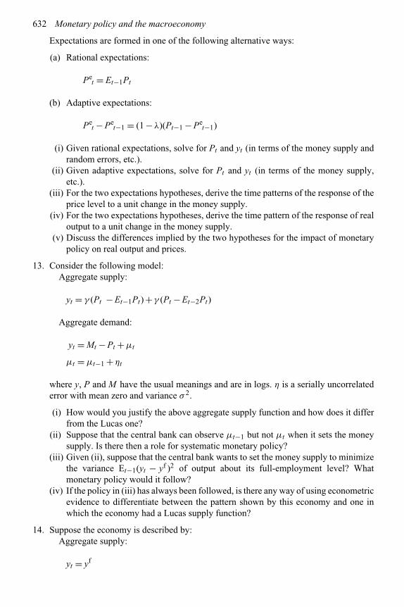
632 Monetary policy and the macroeconomy
Expectations are formed in one of the following alternative ways:
(a) Rational expectations:
Pet = Et−1Pt
(b) Adaptive expectations:
Pet − Pe
t−1 = (1 −λ)(Pt−1 − Pet−1)
(i) Given rational expectations, solve for Pt and yt (in terms of the money supply andrandom errors, etc.).
(ii) Given adaptive expectations, solve for Pt and yt (in terms of the money supply,etc.).
(iii) For the two expectations hypotheses, derive the time patterns of the response of theprice level to a unit change in the money supply.
(iv) For the two expectations hypotheses, derive the time pattern of the response of realoutput to a unit change in the money supply.
(v) Discuss the differences implied by the two hypotheses for the impact of monetarypolicy on real output and prices.
13. Consider the following model:Aggregate supply:
yt = γ (Pt − Et−1Pt) + γ (Pt − Et−2Pt)
Aggregate demand:
yt = Mt − Pt +μt
μt = μt−1 +ηt
where y, P and M have the usual meanings and are in logs. η is a serially uncorrelatederror with mean zero and variance σ 2.
(i) How would you justify the above aggregate supply function and how does it differfrom the Lucas one?
(ii) Suppose that the central bank can observe μt−1 but not μt when it sets the moneysupply. Is there then a role for systematic monetary policy?
(iii) Given (ii), suppose that the central bank wants to set the money supply to minimizethe variance Et−1(yt − yf )2 of output about its full-employment level? Whatmonetary policy would it follow?
(iv) If the policy in (iii) has always been followed, is there any way of using econometricevidence to differentiate between the pattern shown by this economy and one inwhich the economy had a Lucas supply function?
14. Suppose the economy is described by:Aggregate supply:
yt = yf

Macro models and perspectives 633
Aggregate demand and fiscal policy:
yt = α0 +α1(Mt − Pt) +α2Et−1(Pt+1 − Pt) +α3zt +μt α1,α2,α3 > 0
zt = γ0 + γ1zt−1 +ηt
Money supply:
Mt = M0 + νt
where all variables are in logs. μ, η and ν are random disturbance terms. y, M and Phave the usual meanings, and z is a real fiscal variable.
Find the equilibrium solutions for yt and Pt . How do systematic or anticipated changesin the nominal money supply M0 affect yt and Pt? How would unanticipated changes inthe nominal money supply Mt affect yt and Pt? How would anticipated and unanticipatedchanges in the fiscal variable affect yt and Pt?
15. Suppose the output supply in the model of question 14 is not the full-employment levelbut is determined by demand. Re-do the answers to question 14.
16. Suppose the supply function in the model of this question 14 is changed to:
yt = yf + γ (Pt − Et−1Pt) γ > 0
Re-do the answers to question 14.17. Suppose the price level in question 14 is fixed at P (making the model a fixed price one,
compared with the preceding flexible price model). Re-do the answers to this question.18. Specify the three types (backward-looking, contemporaneous and forward-looking) of
the Taylor rule on interest rates, and discuss their validity. Why does the forward-lookingform implied by the new Keynesian model seem to do badly relative to the others, andespecially relative to the backward-looking one?
19. Write the general dynamic form of the sticky-price new Keynesian Phillips curve as:
πt = βEtπt+1 +α(ut − un) + vt
where π is the inflation rate, u is the unemployment rate, un is the natural rate, vt =ρvt−1 +ηt and η is a random variable with a zero mean and constant variance. Mankiw(2001) argues that this relationship is not valid and that the general form of the validrelationship is backward-looking in inflation. Its corresponding form would then be:
πt = βπt−1 +α(ut − un) + vt
Is this form consistent with the original Phillips curve? Provide the theoreticaljustification for it offered by the sticky information model, and critically evaluate thiscontribution.
20. Given the generally poor performance of the forward-looking forms of the Taylor rule andthe Phillips curve implied by the NK model, especially relative to their backward-lookingsimpler versions, discuss whether the new Keynesian reformulation of Keynesianism hasproved to be a failure. If this is so, are there any elements of the NK ideas that shouldbe preserved in further research?

634 Monetary policy and the macroeconomy
References
Ball, L. “Policy rules for open economies.” In J.B. Taylor, ed., Monetary Policy Rules. Chicago: ChicagoUniversity Press, 1999.
Ball, L. “Policy rules and external shocks.” NBER Working Paper no. 7910, 2000.Ball, L., and Mankiw, N.G. “A sticky-price manifesto.” Carnegie-Rochester Series on Public Policy,
41, 1994, pp. 127–51.Barro, R.J. “Unanticipated money growth and unemployment in the United States.” American Economic
Review, 67, 1977, pp. 101–16.Bernanke, B.S., and Woodford, M. “Inflation forecasts and monetary policy.” Journal of Money, Credit
and Banking, 29, 1997, pp. 653–84.Bullard, J., and Keating, J.W. “The long-run relationship between inflation and output in postwar
economies.” Journal of Monetary Economics, 36, 1995, pp. 477–96.Chu, J., and Ratti, R.A. “Effects of unanticipated monetary policy on aggregate Japanese output: the
role of positive and negative shocks.” Canadian Journal of Economics, 30, 1997, pp. 722–41.Clarida, R., Gali, J. and Gertler, M. “The science of monetary policy: a new Keynesian perspective.”
Journal of Economic Literature, 37, 1999, pp. 1661–707.Cover, J.P. “Asymmetric effects of positive and negative money shocks.” Quarterly Journal of
Economics, 107, 1992, pp. 1261–82.Depalo, D. “Japan: the case for a Taylor rule? A simple approach.” Pacific Economic Review, 11, 2006,
pp. 527–46.Friedman, M., and Schwartz, A.J. A Monetary History of the United States, 1867–1960. Princeton, NJ:
Princeton University Press, 1963.Frydman, R., and Rappoport, P. “Is the distinction between anticipated and unanticipated growth
relevant in explaining aggregate output?” American Economic Review, 77, 1987, pp. 693–703.Gali, J. “How well does the IS–LM model fit post-war U.S. data?” Quarterly Journal of Economics,
107, 1992, pp. 709–38.Gali, J. and Gertler, M. “Inflation dynamics: a structural econometric analysis.” Journal of Monetary
Economics, 44, 1999, pp. 195–222.Levin, A.T., Wieland, T.V. and Williams, J.C. “Robustness of simple monetary policy rules under
model uncertainty.” In J.B. Taylor, ed., Monetary Policy Rules. Chicago: University of Chicago,1999, pp. 263–99.
Levin, A.T., Wieland, T.V. and Williams, J.C. “The performance of forecast-based monetary policyrules under model uncertainty.” Federal Reserve System Working Paper no. 2001-39, 2001.
Lucas, R.E., Jr. “Expectations and the neutrality of money.” Journal of Economic Theory, 4, 1972,pp. 103–24.
Lucas, R.E., Jr. “Some international evidence on output–inflation tradeoffs.” American EconomicReview, 63, 1973, pp. 326–34.
Lucas, R.E., Jr. “Comments on Ball and Mankiw.” Carnegie-Rochester Series on Public Policy, 41,1994, pp. 153–5.
Lucas, R.E., Jr. “Nobel lecture: monetary neutrality.” Journal of Political Economy, 104, 1996,pp. 661–82.
Mankiw, N.G. “The inexorable and mysterious tradeoff between inflation and unemployment.”Economic Journal, 111, 2001, pp. C45–C61.
Mankiw, N.G., and Reis, R. “Sticky information versus sticky prices: a proposal to replace the newKeynesian Phillips curve.” Quarterly Journal of Economics, 117, 2002, pp. 1295–328.
Mankiw, N.G., and Reis, R. “ Pervasive stickiness.” American Economic Review, 96, 2006a, pp. 164–9.Mankiw, N.G., and Reis, R. “ Sticky information in general equilibrium.” NBER Working Paper no.
12605, 2006b.Maria-Dolores, R., and Vazquez, J. “How does the new Keynesian monetary model fit in the
U.S. and the Eurozene? An indirect inference approach.” Topics in Macroeconomics, 6, 2006,article 9, pp. 1–49.

Macro models and perspectives 635
Mishkin, F.S. “Does anticipated aggregate demand policy matter? Some further econometric results.”American Economic Review, 72, 1982, pp. 788–802.
Mosser, P. “Changes in monetary policy effectiveness: evidence from large macroeconomic models.”Federal Reserve Board of New York Quarterly Review, 17, 1992, pp. 36–51.
Rudd, J., and Whelan, K. “Can rational expectations sticky price models explain inflation dynamics?”At www.federalreserve.gov/pubs/feds/2003/200346, 2003.
Sargent, T.J., and Wallace, N. “Rational expectations and the theory of economic policy.” Journal ofMonetary Economics, 2, 1976, pp. 169–83.
Wang, S., and Handa, J. “Monetary policy rules under a fixed exchange rate regime: empirical evidencefrom China.” Applied Financial Economics, 17, 2007, pp. 941–50.

18 Walras’s law and the interaction amongmarkets
This chapter focuses on Walras’s law, which is fundamental to macroeconomic analysis.It underlies the IS–LM model, which has four goods – commodities, money, bonds andlabor – but has explicit analysis of only three of them. The foundations of Walras’s law and itsvalidity in disequilibrium are rigorously examined in this chapter. This is also done for Say’slaw. The analyses of Walras’s and Say’s laws are followed by the derivation of their jointimplications for the dichotomy between the real and the monetary sectors, and the neutrality ofmoney.
The Pigou and real balance effects concern the impact of changes, brought about by changesin the price level, in the value of financial assets and of real balances, respectively, on thedemand for commodities. They played a key role in doctrinal disputes on whether an economyfunctioning below full employment would return to full employment. This chapter examinestheir nature and empirical relevance.
These discussions are followed by analyses of effective Clower and Drèze demand andsupply functions versus notional ones.
Key concepts introduced in this chapter
♦ A law versus an equilibrium condition♦ Walras’s law♦ Say’s law♦ Dichotomy between real and monetary sectors♦ Pigou effect♦ Real balance effect♦ Notional demand and supply functions♦ Clower effective demand and supply functions♦ Drèze functions
There are very few propositions in economics that have been considered to be so far beyonddispute as to be labeled “laws.” Among these are Walras’s law and Say’s law. The formerrepresents a constraint on all goods in the economy while the latter represents a constraint onthe commodity market alone. This chapter will consider these laws for the closed economy,though the arguments can be easily extended to the open economy.
A statement in economics worthy of being called a law must be more than a behavioralrelationship or an equilibrium condition – both of which are not necessarily valid at agiven time for a given economy – since, otherwise, there would not be a special reason

Walras’s law 637
for assigning it a distinctive term with the compelling connotation that the word “law”possesses. Hence, while there can be several ways of defining what can be designated as alaw in economics, we will define it as a statement that holds without exception under anyand all conditions, so that it is an identity – or, if one is willing to be more tolerant, it mustbe a statement that approximates this degree of applicability. There are very few statementsof this nature in microeconomics, let alone in macro or monetary economics.1 The classicalparadigm asserts that Walras’s law is one of this extremely select group. However, as wediscuss in Section 18.8 below, there are serious and well-founded arguments against itsbeing a law or an identity. In particular, while it holds in the general equilibrium statesof the economy, its implications for the dynamic analysis of prices, wages and interestrates need not be always valid. Hence, we conclude that it is not an identity and, therefore,not a law.
Say’s law asserts that the supply of commodities creates an equal demand for them. Thischapter shows that it does not hold as an identity in the modern economy with financial assets,so that it is clearly not a law for the modern economy. It really should not be a part of anymodern macroeconomic analysis.
Sections 18.1 to 18.3 present the derivation of Walras’s law and its implications.Section 18.4 deals with Say’s law and finds it inappropriate for monetary economies.Section 18.5 discusses the implications of the joint assumption of Walras’s law and Say’slaw for the neutrality of money and the dichotomy between the real and monetary sectors.Sections 18.6 and 18.7 present the wealth and real balance effects. Both these concepts havealready been presented in Chapter 3 in the context of the Walrasian general equilibriummodel of the economy. Sections 18.8 to 18.12 examine the conditions for the breakdown ofWalras’s law and the implications of this breakdown.
18.1 Walras’s law
Walras’s law is the statement that for any economy, over any given period of time, the sum ofthe market values of all the goods demanded must equal the sum of the market values of allthe goods supplied. For the closed economy,2 we define “goods” in this chapter, as in earlierchapters, to refer to commodities, money, labor (or leisure) and non-monetary financial assets(“bonds”).
To explain Walras’s law intuitively for a pure exchange economy, first start with theconstraint on the individual’s demands for goods. Assume that the individual initiallypossesses some commodities, some money and some bonds,3 and that their total nominalvalue at current market prices is his nominal wealth ψ . He will also want to supply somelabor, with a nominal labor income at current wage rates being equal to Y . Assuming thathe spends this amount to acquire the commodities, money and bonds that he wants to hold
1 Another proposition that is sometimes referred to as a law is the “law of one price,” which in international tradetranslates to absolute purchasing power parity between countries. However, it is often rejected by empiricalevidence, so that it cannot be properly regarded as a law.
Another proposition often labelled as a law is that “the demand curves for commodities slope downwards.”However, this is violated for many goods, such as those with snob appeal, which have upward-sloping demandcurves. Therefore, even this proposition is not an identity and not really a law.
2 The open economy has an additional good in the form of foreign exchange held by the private and public sectors.3 Bond holdings can be positive (making the individual a net lender) or negative (making the individual a net
borrower).

638 Monetary policy and the macroeconomy
or use in the current period,4 the total value ψ of his initial holdings of goods plus his laborincome Y must equal his total expenditures on commodities, money and bonds. Since theindividual’s total expenditures on his purchases of commodities, money and bonds must sumto [ψ + Y ], the demand for any one of these three goods can be derived by subtracting hisexpenditures for the other two goods from [ψ + Y ].
If we now sum over all the individuals in the economy, the aggregate initial holdingsof goods (including labor) plus the current national output becomes their supply and theaggregate expenditures on them become the value of the quantities demanded. Further, thetotal value of all the goods demanded must equal the total value of all the goods supplied.This is Walras’s law, and it is the aggregate counterpart of the individual’s budget constraint.It is often simplified to the statement that the supply of all goods in the economy must equalthe demand for all goods in the economy.
Deriving Walras’s law for a five-good closed economy
We prove Walras’s law for a closed economy with a government sector and for its fivegoods – commodities, money, bonds, equities, and labor.5 The assumption basic to Walras’slaw is that there is no “free” disposal of goods (i.e. economic agents do not just throw themaway) so that the goods that are produced or inherited from the past are either consumed,demanded for some other reason (such as for carrying to the future as saving in the form ofcommodities) or exchanged against money or bonds. Assume that the closed economy hasthree economic agents – households, firms and the government (including the central bank) –so that there are several budget constraints to consider in the analysis. The definitions of thesymbols in the constraints are given after the specification of the constraints, which are asfollows.
HOUSEHOLDS’ BUDGET CONSTRAINT
This constraint specifies that the payments by households for all goods (commodities, money,bonds and equities) bought must equal the funds available from the initial endowments (i.e.inherited stocks) of goods, labor income and the profits received from firms as distributedprofits. That is:
pccdh + pcm
dh + pbbd + peed ≡ pcc
s + M h + pbbs + pees + Wns +πdis (1)
FIRMS’ BUDGET CONSTRAINTS
Firms face three constraints. The first one specifies that the funds available to the firms fromthe sales of their products (to households for consumption, to other firms for investment andto government) and of new equities must equal the sum of the payments to the labor employedand funds used for the firm’s investments, money holdings or distributed profits. The firms’second constraint specifies that total profits can be either distributed or retained/undistributed
4 We have assumed that the individual is a supplier of labor services and firms are the buyers of such services.5 We have included three financial goods, money, bonds and equities, in the following analysis in order to show
that the separate treatment of equities does not destroy Walras’s law. Note that in the rest of this book and inmonetary economics generally, “bonds” are defined to include all non-monetary assets and therefore would alsoinclude equities.

Walras’s law 639
by the firm. The third constraint specifies that the firm’s investment must be financed fromits retained earnings and the issue of new equities.
pc (csh + i + g) + pe (es − es) + M f ≡ Wnd + pc i + pc mdf +πdis (2)
π ≡ πdis +πundis (3)
pci ≡ πundis + pe (es − es) (4)
GOVERNMENT’S BUDGET CONSTRAINT
This constraint specifies that the government must finance its deficits or surpluses by theissue of new money and bonds.
pc (g − t) ≡ (M s − M s) + pb (bs − bs) (5)
The definitions of the symbols in the preceding five identities are:
pc price of commoditiespb price of government bondspe price of equitiesW nominal wage rate = rental price
of laborcsh supply of commodities to
householdscsf total supply of commodities by
firms (≡ csh + i + g)m real money balancesM nominal money stockb quantity of bondse quantity of equitiesn number of workers (labor)c existing stocks of commodities
(held by households)
M existing nominal money stock(held by households and firms)
b existing stock of bonds (issuedby the government, held byhouseholds)
e existing stock of equities (issuedby firms, held by households)
g real government expenditures oncommodities
t government’s tax revenuesi real investment by firmsπ total nominal profits of firmsπdis nominal distributed profitsπundis nominal retained (undistributed)
profits of firms
The superscripts d and s stand for demand and supply respectively. The superscriptsh and f stand for households and firms respectively. Underlining indicates that the valueof the variable is given exogenously or was inherited from the past. Note that cd ≡cdh + i + g, cs ≡ csf + cs and M ≡ M h + M f . For simplification, (1) to (5) makethe usual assumption that only firms issue equities and that only the government issuesbonds.
Note that (1) to (5) are all identities, designated by the use of the symbol ≡, and resultfrom the assumption that nothing is just thrown away by economic agents since doing sowould be irrational. They imply that:
pc (cd − cs) + (M d − M s) + pb (bd − bs) + pe (ed − es) + W (nd − ns) ≡ 0 (6)
where the left-hand side is the sum of the nominal excess demands for commodities, money,bonds, equities and labor. (6) is one of the ways of stating Walras’s law: the sum of the
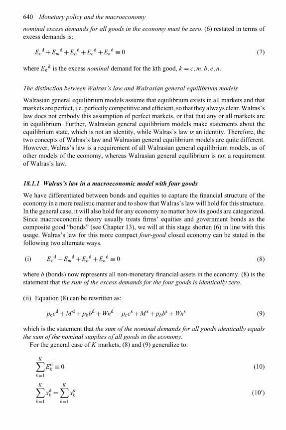
640 Monetary policy and the macroeconomy
nominal excess demands for all goods in the economy must be zero. (6) restated in terms ofexcess demands is:
Ecd + Em
d + Ebd + Ee
d + End ≡ 0 (7)
where Ekd is the excess nominal demand for the kth good, k = c,m,b,e,n.
The distinction between Walras’s law and Walrasian general equilibrium models
Walrasian general equilibrium models assume that equilibrium exists in all markets and thatmarkets are perfect, i.e. perfectly competitive and efficient, so that they always clear. Walras’slaw does not embody this assumption of perfect markets, or that that any or all markets arein equilibrium. Further, Walrasian general equilibrium models make statements about theequilibrium state, which is not an identity, while Walras’s law is an identity. Therefore, thetwo concepts of Walras’s law and Walrasian general equilibrium models are quite different.However, Walras’s law is a requirement of all Walrasian general equilibrium models, as ofother models of the economy, whereas Walrasian general equilibrium is not a requirementof Walras’s law.
18.1.1 Walras’s law in a macroeconomic model with four goods
We have differentiated between bonds and equities to capture the financial structure of theeconomy in a more realistic manner and to show that Walras’s law will hold for this structure.In the general case, it will also hold for any economy no matter how its goods are categorized.Since macroeconomic theory usually treats firms’ equities and government bonds as thecomposite good “bonds” (see Chapter 13), we will at this stage shorten (6) in line with thisusage. Walras’s law for this more compact four-good closed economy can be stated in thefollowing two alternate ways.
(i) Ecd + Em
d + Ebd + En
d ≡ 0 (8)
where b (bonds) now represents all non-monetary financial assets in the economy. (8) is thestatement that the sum of the excess demands for the four goods is identically zero.
(ii) Equation (8) can be rewritten as:
pccd + M d + pbbd + Wnd ≡ pcc
s + M s + pbbs + Wns (9)
which is the statement that the sum of the nominal demands for all goods identically equalsthe sum of the nominal supplies of all goods in the economy.
For the general case of K markets, (8) and (9) generalize to:
K∑k=1
Edk ≡ 0 (10)
K∑k=1
xdk =
K∑k=1
xsk (10′)
Walras’s law 641
where xk is the quantity of the kth good and there are K goods in the economy. (10) or (10′)is the general statement of Walras’s law.
Adjustment costs, which slow the adjustment in the demands and/or supplies of goods sothat their short-run values differ from their long-run ones, do not change the derivationor applicability of Walras’s law, nor does the introduction of uncertainty and rationalexpectations into the model. However, the validity of Walras’s law for dynamic analysisdoes become questionable if the labor and commodity markets do not clear on a continuousbasis. Sections 18.8 to 18.10 will examine this issue.
18.1.2 The implication of Walras’s law for a specific market
Walras’s law by itself does not assert equilibrium in each market or in any one specificmarket, but is a statement covering all markets in the economy. (10) implies that:
EKd ≡ −
K−1∑k=1
Edk (11)
where EKd is excess demand in the K th market. This condition asserts that the excess nominal
demand in the K th market equals the sum of the excess nominal demands in the other (K−1)markets, where we can arbitrarily designate the market for any specific good as the K thmarket. (11) implies that:
If Ekd = 0, fork = 1,...,K − 1, then EK
d = 0 (12)
That is, if there exists equilibrium in K − 1 markets, then there would also be equilibriumin the K th market. (12) is also sometimes used as a way of stating Walras’s law. In generalequilibrium analysis, (11) and (12) allow the analysis to dispense with the explicit treatmentof one of the markets in the economy. Note, however, that such an omitted market continues toexist and to function but its treatment is pushed into the implicit state. Further, the solution ofany of the three markets for the three prices (P,pb,W ) in (9) would be identical, irrespectiveof which market is omitted from the explicit analysis. Furthermore, the general equilibriumvalues of the real variables, such as output, employment, consumption, etc., will also beidentical.
18.2 Walras’s law and selection among the markets for a model
Implications of Walras’s law for general equilibrium analysis
As shown above, Walras’s law permits the general equilibrium conditions for any threeout of the four goods in the closed-economy macroeconomic model to be explicitlyspecified for the solution of the overall equilibrium of the economy. Therefore, thecomplete model can explicitly set out the equations for any of the following four groups ofmarkets:
(I) commodities, money and labor markets;(II) bond, money and labor markets;

642 Monetary policy and the macroeconomy
(III) commodities, bond and labor markets;(IV) commodities, money and bond markets;
Grouping I was used by Keynes, and has become the standard set used in modernmacroeconomics. The neoclassical and the modern classical models also follow this pattern.As is discussed in greater detail in Chapter 19, the traditional classical economists, priorto Keynes, had generally favored grouping II, with the bond market determining theinterest rate in the loanable funds theory, the market for money determining the pricelevel by the quantity theorem, and the labor market determining employment and –through the production function – determining output. Walras’s law implies that each ofthe above sets would provide the same general equilibrium solution of the values of theendogenous variables, even though the explicitly specified three markets differ betweenthe sets.
Implications of Walras’s law for the dynamic analysis of markets
While the different approaches may yield the same general equilibrium values of thevariables, the general pattern of economic analysis identifies a “price” variable with eachmarket. Thus, the price level is the “price” of commodities, and microeconomic analysisidentifies its determination with the demand and supply of commodities. The interest rate issimilarly the one-period “price” of loans/bonds, and microeconomic analysis would identifyits determination by the market for loans/bonds. The wage rate is the rental price of labor,and microeconomic analysis identifies its determination with the labor market. Hence, thereis no “price” left to identify as the price of money, so that there is no price variable that canbe uniquely identified with the demand and supply of money. There can, in fact, be no suchunique variable in a monetary economy since money is itself the good in which the prices ofother goods (commodities, bonds and labor) are measured. Thus, 1/P is sometimes said tobe the value of money(in commodity units) while, at other times, the interest rate is said tobe its opportunity cost, and many pre-Keynesian economists designated its value (in laborunits) as 1/Pw.
This reasoning suggests that, if a model is to capture the dynamic movements ofprices, wages and the interest rate in real-world markets, it needs to take account ofthe empirical reality that the price of a particular good responds in the first instanceto the excess demand only in the market for that good. This price should not respond tothe excess demands for other goods, unless these demands spill over into the excess demandfor the good in question. Therefore, for dynamic analysis, the appropriate assumptionswould be:
∂Pt/∂t = f (Ectd)
∂Rt/∂t = f (Ebtd)
∂Wt/∂t = f (Entd)
where R is the nominal yield on bonds. These dynamic functions seem to be consistentwith common intuition and economic folklore on price adjustments in markets. Severalstudies of the dynamic analysis of the price level and the interest rate have in recent yearsfollowed this pattern: that is, making changes in the price level a function of the commodity