Monash Freeway Upgrades Stage 2 Economic …roadprojects.vic.gov.au › __data › assets ›...
67
www.pwc.com.au Monash Freeway Upgrades Stage 2 Economic Assessment Report VicRoads Monash Freeway Upgrade Stage 2, Economic Assessment Report March 2018
Transcript of Monash Freeway Upgrades Stage 2 Economic …roadprojects.vic.gov.au › __data › assets ›...
www.pwc.com.au
Monash Freeway Upgrades Stage 2 Economic Assessment Report
VicRoads
Monash Freeway
Upgrade Stage 2,
Economic Assessment
Report
March 2018

Disclaimer
This report is a confidential document that has been prepared by PricewaterhouseCoopers (PwC) at the request of VicRoads in connection with our contract to provide commercial and financial advice in relation to the development of a Business Case for the proposed Monash Freeway Upgrade Stage 2 Project (the Project).
The analysis contained in this report has been prepared by PwC from, inter alia, material provided by, and discussions with, VicRoads and third parties including:
Aquenta
WSP
Department of Treasury and Finance (DTF)
Department of Economic Development, Transport, Jobs and Resources (DEDTJR)
Transport for Victoria (TfV)
(together, the Information).
No verification of the Information has been carried out by PwC or any of its respective agents, directors, officers, contractors or employees, and in particular PwC has not undertaken any review of the financial information supplied or made available during the course of the engagement. This report does not purport to contain all the information that VicRoads may require in considering the Project or its procurement.
PwC has based this report on Information received or obtained, on the basis that such Information is accurate and, where it is represented, complete. PwC and its respective agents, directors, officers, contractors and employees make no express or implied representation or warranty as to the accuracy, reliability or completeness of the Information.
PwC will not provide any express or implied opinion (and assumes no responsibility) as to whether actual results will be consistent with, or reflect results of, any financial model outputs.
PwC may in its absolute discretion, but without being under any obligation to do so, update, amend or supplement the Information.
This report is for the sole use of VicRoads in considering the Project and its procurement. The information contained in this paper is strictly confidential and must not be copied, reproduced, distributed, disseminated or used, in whole or in part, for any purpose other than as detailed above without PwC’s express written permission.
Liability limited by a scheme approved under Professional Standards Legislation.

VicRoads PwC i
Contents
Disclaimer i
Executive summary 1
1 Introduction 3
2 Nature of the Economic Assessment 4
3 Scenarios Assessed 10
4 Land Use and Demand Forecast 13
5 Costs 20
6 Benefits 21
7 Economic Analysis Results 51
Appendices 56
Appendix A Vehicle Operating Cost – Austroads 2012 methodology
Appendix B Wider Economic Benefits

VicRoads PwC 1
Executive summary
Purpose of this document This report presents an economic assessment of potential investment in Melbourne’s transport network being considered by the Victorian Government and the Commonwealth Government in relation to problems identified along the Monash Freeway Corridor. Both the Victorian Government and the Commonwealth Government have agreed to each fund $500 million to invest in the Freeway and based on this agreement Stage 1 of the Monash Freeway Upgrade project has already been funded. The purpose of the analysis in this report is to identify a preferred scope for Stage 2 investments.
PricewaterhouseCoopers Consulting Australia Pty Ltd (PwC) has been commissioned by VicRoads to undertake an economic assessment of the Project. This document sets out the methodology and findings of the economic assessment. This report should be read in conjunction with the Monash Freeway Upgrade Stage 2 Business Case.
Economic assessment of the Project Methodology Based on the strategic options assessment, the scope of works for the Monash Freeway Upgrade Project under stage 2 is together referred to as ‘the Project’.
The Project will generate a number of benefits for road users and the Melbourne community. The benefits of the Project include improved network efficiency, reduced congestion, enhanced freight efficiency and improved accessibility along Melbourne’s south-east and outer south-east corridor. The Project will also increase the resilience of Melbourne’s road network and improve liveability and amenity through reduced crashes and improved air quality. These benefits will generate wider economic benefits through improved accessibility to key employment clusters.
A cost benefit analysis (CBA) framework has been applied to estimate net economic benefits based on current Victorian practice, taking into account Victorian Government guidelines1 and the Victorian Auditor-General’s Office recommendations for traffic modelling.2 To align with Commonwealth Government guidelines, the CBA results have also been calculated as sensitivity based on Infrastructure Australia’s June 2017 published economic guidelines.3
An overarching requirement of most economic appraisal guidelines and fundamental principal of CBA is to measure the impact on the community as a whole. This involves identifying and, where possible, quantifying the costs and benefits directly attributable to an initiative.4 As a result, where considered to reflect the nature of this Project, and supported by economic theory and guidelines, along with appropriate parameters for quantification, project-specific benefits have been included in the appraisal.
Results of the detailed economic assessment The economic assessment of the preferred Bundle 3A and Bundle 3B indicates strong economic results in terms of traditional transport benefits (including travel time savings, vehicle operating cost savings and improved network resilience) and also wider economic benefits and relief in terms of the perceived value of congestion. Bundle 3A, which provides the improved access to the south-east
1 DEDJTR Guidelines for Transport Modelling and Economic Appraisal in Victoria (v3.03 May 2017) and DTF (2013) Economic Evaluation for
Business Cases Technical Guidelines, August 2013
2 Victorian Auditor General, 2011, Management of Major Road Projects
3 Infrastructure Australia, 2017 Assessment Framework
4 Infrastructure Australia, 2014, Better Infrastructure Decision-Making, available at:
http://infrastructureaustralia.gov.au/projects/files/Reform_and_Investment_Framework_Guidance.pdf; Victorian Department of Treasury and Finance, 2013, Investment Lifecycle and High Value/ High Risk Guidelines (Stage 2 – Prove - Economics evaluation technical guide), updated August 2013, p 6
VicRoads PwC 2
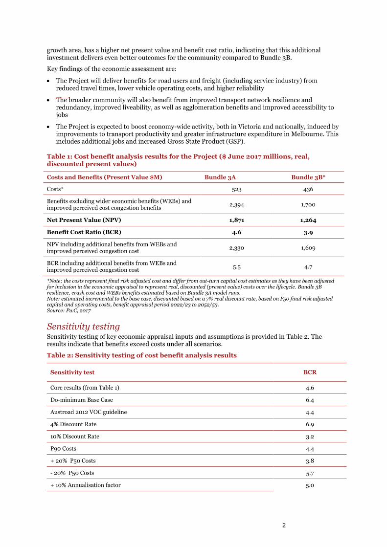
growth area, has a higher net present value and benefit cost ratio, indicating that this additional investment delivers even better outcomes for the community compared to Bundle 3B.
Key findings of the economic assessment are:
The Project will deliver benefits for road users and freight (including service industry) from reduced travel times, lower vehicle operating costs, and higher reliability
The broader community will also benefit from improved transport network resilience and redundancy, improved liveability, as well as agglomeration benefits and improved accessibility to jobs
The Project is expected to boost economy-wide activity, both in Victoria and nationally, induced by improvements to transport productivity and greater infrastructure expenditure in Melbourne. This includes additional jobs and increased Gross State Product (GSP).
Table 1: Cost benefit analysis results for the Project ($ June 2017 millions, real, discounted present values)
Costs and Benefits (Present Value $M) Bundle 3A Bundle 3B*
Costs* 523 436
Benefits excluding wider economic benefits (WEBs) and improved perceived cost congestion benefits
2,394 1,700
Net Present Value (NPV) 1,871 1,264
Benefit Cost Ratio (BCR) 4.6 3.9
NPV including additional benefits from WEBs and improved perceived congestion cost
2,330 1,609
BCR including additional benefits from WEBs and improved perceived congestion cost
5.5 4.7
*Note: the costs represent final risk adjusted cost and differ from out-turn capital cost estimates as they have been adjusted for inclusion in the economic appraisal to represent real, discounted (present value) costs over the lifecycle. Bundle 3B resilience, crash cost and WEBs benefits estimated based on Bundle 3A model runs. Note: estimated incremental to the base case, discounted based on a 7% real discount rate, based on P50 final risk adjusted capital and operating costs, benefit appraisal period 2022/23 to 2052/53. Source: PwC, 2017
Sensitivity testing Sensitivity testing of key economic appraisal inputs and assumptions is provided in Table 2. The results indicate that benefits exceed costs under all scenarios.
Table 2: Sensitivity testing of cost benefit analysis results
Sensitivity test BCR
Core results (from Table 1) 4.6
Do-minimum Base Case 6.4
Austroad 2012 VOC guideline 4.4
4% Discount Rate 6.9
10% Discount Rate 3.2
P90 Costs 4.4
+ 20% P50 Costs 3.8
- 20% P50 Costs 5.7
+ 10% Annualisation factor 5.0

VicRoads PwC 2
Sensitivity test BCR
- 20% Annualisation factor 4.1
+ 20% Benefits 5.6
- 20% Benefits 3.7
Exclude escalation (above real growth) 4.0
Construction Disruption Impact 4.1
Best Case: P50 cost, do-minimum base case, +10% annualisation, ATAP VOC approach
7.0
Worst Case: P90 cost, do-minimum base case, -10% annualisation, Austroad VOC approach
3.3
Note: unless specified estimated incremental to the Base Case, discounted based on a 7% real discount rate, based on P50 capital and operating costs, benefit appraisal period FY23 to FY52, excludes WEBS and improved perceived congestion benefit. Source: PwC, 2017
VicRoads PwC 3
1 Introduction
1.1 Background Melbourne’s south-east and outer south-east5 (the Region) is home to two National Employment and Innovation Clusters (NEICs), Monash and Dandenong, and also key health and education precincts such as Monash Medical Centre, Dandenong Hospital and Monash University. This is a State significant economic region for Melbourne and Victoria, connecting residents and businesses to local, national and international markets vital for economic development, employment, and education. Without further investment, the infrastructure in the Monash Transport Corridor which underpins the movement of people and goods to, from and within this Region will face a number of major problems. Keys problems include increasing congestion and travel times, and diminishing access to strategic employment, education and health clusters.
Acknowledging the many challenges the Region will face, both the Victorian Government and the Commonwealth Government agreed to each fund $500 million to invest in the Freeway and based on this agreement Stage 1 of the Monash Freeway Upgrade project has already been funded. The purpose of the analysis in this report is to identify a preferred scope of Stage 2 investments (“Project”).
PricewaterhouseCoopers Consulting Australia Pty Ltd (PwC) has been commissioned by VicRoads to undertake an economic assessment of the Project.
1.2 Purpose of this document This report sets out the economic assessment undertaken by PwC on behalf of the State and Commonwealth to evaluate the project scope. The purpose of this report is to document the methodology and results of the economic assessment. This report should be read in conjunction with the Monash Freeway Upgrade Stage 2 Business Case.
The remainder of this report is structured as follows:
Chapter 2: Nature of the economic assessment – this chapter presents the overarching methodology and key assumptions for the economic assessment
Chapter 3: Scenarios assessed – this chapter defines the project scope and options evaluated in the economic assessment
Chapter 4: Land use and demand forecasts– this chapter outlines methodology, key assumptions and outputs of the demand forecasting model along with its underlying land use assumptions
Chapter 5: Costs – this chapter outlines the capital costs, operating and maintenance costs of the Project
Chapter 6: Benefits – this chapter presents detailed methodology of the benefit estimation
Chapter 7: Economic analysis results – this chapter presents the results of the economic assessment.
Appendix A Vehicle operating cost - Austroads methodology
Appendix B Wider economic benefits
5 Melbourne’s south-east and outer south-east is defined in this business case as the Bayside, Boroondara, Casey, Cardinia, Frankston, Glen
Eira, Greater Dandenong, Kingston, Knox, Monash, Stonnington and Whitehorse Local Government Areas

VicRoads PwC 4
2 Nature of the Economic Assessment
An overarching requirement of most economic assessment guidelines is that a cost benefit analysis (CBA) framework be applied in order to measure the impact on welfare considering the change in consumer surplus and producer surplus attributable to a transportation or other improvement.
To measure the impact on the community as a whole, a fundamental principal of a CBA is that all costs and benefits attributable to the project should be identified and quantified where possible.67 However economist are principally constrained by the advancement of methodologies, and development of parameters for measurement and monetisation, in order to fully capture the full range of benefits and costs of an initiative. As a result, where considered to reflect the nature of this project, project-specific benefits have been included in the assessment in line with latest guidelines from transport assessment authorities such Infrastructure Australia, Transport and Infrastructure Council etc.
This chapter provides a summary of each form of assessment and sets out the key assumptions and parameters applied.
2.1 CBA framework applied CBA is an appraisal framework that allows costs and benefits of an initiative that fall across different members of the community – potentially at different points in time – to be compared in a consistent fashion.
The main steps of a CBA, outlined in Figure 1, represent the CBA methodology applied to the Project.
6 Infrastructure Australia, 2014, Better Infrastructure Decision-Making, available at:
http://infrastructureaustralia.gov.au/projects/files/Reform_and_Investment_Framework_Guidance.pdf
7 Victorian Department of Treasury and Finance, 2013, Investment Lifecycle and High Value/ High Risk Guidelines (Stage 2 – Prove -
Economics evaluation technical guide), updated August 2013, p 6.

VicRoads PwC 5
Figure 1: CBA framework adopted
Source: PwC, 2017
2.2 Alignment with State and National Guidelines The economic appraisal has been developed based on Australian guidelines and current Victorian practice, and draws upon Australian and international research papers.
The CBA methodology has been developed in consideration with the following Australian guidelines:
Victorian Department of Economic Development Jobs, Transport and Resources (DEDJTR) Guidelines for Transport Modelling and Economic Appraisal in Victoria v3.03 May 2017 (‘DEDJTR 2017 Guidelines’)
Victorian Department of Treasury and Finance (DTF), Investment Lifecycle and High Value/ High Risk Guidelines (Stage 2 Prove economics evaluation technical guide), updated August 2013 (‘Vic DTF 2013 HVHR’)
Australian Transport Council National Guidelines for Transport System Management in Australia, 2006, 5 volumes8 (‘ATC 2006 NGTSM’)
Transport and Infrastructure Council, 2016, Australian Transport Assessment and Planning Guidelines– (‘ATAP 2016 Guidelines’)
8 A draft update to the ATC 2006 National Guidelines for Transport System Management in Australia has been released for stakeholder
comment, but final guidelines have not been released as at September, 2015, and so the updated guidelines have not been applied.
1. Set overall appraisal
framework
• Identify relevant appraisal guidelines• Establish appraisal period, discount rate and other overarching assumptions / parameters
2. Without-project and
project cases
• Define a base case in terms of when transport infrastructure will be implemented• Define Project options
3. Land use and demand forecasting
• Define land use assumptions without transport project network• Transport modellers reflect future demographics and transport infrastructure with and without the
project and estimate transport outcomes in given forecast years• Develop an approach to 'extract' transport outcome measures from the demand model (e.g. travel times
and vehicle kilometres travelled) with and without the project in given forecast years• Apply an appropriate annualisation factor to convert average weekday forecasts to annual estimates• Interpolate and extrapolate forecasts of outcomes to develop a full time profile of outcomes over time
4. Quantify economic
costs
• For Base Case and Project Case, estimate capital and operating costs• Collate incremental costs in each future year (capital and recurrent)• Adjust financial cost for resource cost correction to estimate economic costs in each year
5. Quantify economic benefits
• Translate incremental transport outcomes with the project to economic benefits by applying appropriate economic unit valuations to these outcomes
• Analyse qualitative impacts unable to be quantified
6. Estimate results
• Convert costs and benefits into their equivalent values at the commencement of the appraisal period using discounting
• Determine if total discounted benefits exceed discounted costs• Calculate the benefit cost ratio (BCR) and the Net Present Value (NPV) by option• Test the BCR against changes to underlying parameter assumptions

VicRoads PwC 6
Infrastructure Australia, 2017 Assessment Framework, (‘IA 2017 Guidelines’)
Infrastructure Australia, Reform and Investment Framework Template, Templates for Stage 7 Solution Evaluation (transport infrastructure), December 20139 (‘IA December 2013 RIF’)
Austroads, Guide to Project Evaluation, 2012, “Part 4: Project evaluation data” (‘Austroads 2012’)
To consider specific methodologies required to estimate benefits (e.g. estimating wider economic benefits, or WEBs), other benefit guidance has been considered from international literature and guidelines, such as:
Victorian Auditor General’s Office (VAGO) recommendations regarding accounting for induced demand when forecasting traffic and estimating economic benefits10
United Kingdom Department for Transport (DfT), Transport Analysis Guidance – WebTAG (‘UK DfT TAG’)
NZ Transport Agency (NZTA), Economic evaluation manual, 2013 (‘NZTA 2013 EEM’)
2.3 Key assumptions and parameters The key appraisal assumptions and parameters presented in Table 3 have been assumed for economic assessment of the Project considering the guidelines outlined above.
9 Infrastructure Australia, 2013, Reform and Investment Framework templates (transport Infrastructure), available at:
http://infrastructureaustralia.gov.au/projects/files/Infrastructure_Priority_List_Submission_Template_ Stage_7_Transport.pdf, accessed 1 July 2015.
10 Victorian Auditor General, 2011, Management of Major Road Projects

VicRoads PwC 7
Table 3: General CBA assumptions
Assumption Source and Comments
Real discount rate
7% (real)
4% and 10% (real) sensitivity tests
DEDJTR Guidelines suggest 7% discount rate be applied for core BCR where 4 and 10% discount rates be applied as sensitivity.
Consistent assumption under IA 2017 Guidelines.
Base price year June 2017 Parameters designated in prices prior to the base price year (e.g. 2009 dollars) are inflated to June 2017 dollars based on the Melbourne Consumer Price Index (CPI),11 Victorian Wage Price Index (WPI),12 and Melbourne Producer Price Index (PPI).13
Consistent assumption under IA 2017 Guidelines.
Construction period
FY 2018/19-2021/22:
Post planning and design, construction will commence in fourth quarter of 2019
Provided by VicRoads and Aquenta
Appraisal period Commences in 2022/23 and extends 30 years from the operation start date of 2022/23 to 2051/52
Vic DTF 2013 HVHR suggest that projects should generally be evaluated over the full lifecycle but agencies might want to limit the evaluation period to a shorter duration such as 30 years. To be conservative and align with IA 2017 Guidelines a 30 year appraisal was assumed.
Residual value Calculated based on straight-line depreciation is used to calculate the replacement cost
Vic DTF 2013 HVHR suggests that when the economic life of an asset exceeds the evaluation period of the project, the residual value can be counted as an inflow of benefits in the last year. The residual value should be the lower of:
– The depreciated replacement cost
– The future stream of net benefits at the arbitrary end of the project (discounted back to the present value along with the other costs and benefits).
IA 2017 Guidelines suggest a preference for straight-line depreciation.
Induced demand For BCR results based induced demand outputs have been used to capture changes in route, mode and destinations as modelled by VITM.
DEDJTR Guidelines assess the significance of induced traffic for all major road projects and take account of this when forecasting traffic and estimating the economic benefits.
Of the six types of induced demand suggested by VAGO (2011), The VITM accounts for three types of behavioural change (mode, route and destination).14
11 ABS, 2017 Series id A2325846C Consumer Price Index, Index Numbers ; All groups CPI ; Australia ; Jun 2017
12 ABS, 2017, Series id A2706258V Wage Price Index, Total hourly rates of pay excluding bonuses ; Victoria ; Private and Public ; All industries
; March 2017
13 ABS, 2017, 6427.0 - Producer Price Indexes, Australia, Jun 2017
14 Victorian Auditor General, 2011, Management of Major Road Projects, page 8

VicRoads PwC 8
Assumption Source and Comments
Escalation Cost
4% per annum for capital cost (includes inflation rate)
3% per annum for operating cost(includes inflation rate)
Productivity Growth
1.5% per annum above real growth for business travel
0.75% per annum above real growth for non-business travel
DEDJTR Guidelines recommend to incorporate real escalation that is in excess of RBA’s inflation target rate on 2.5%. The escalation rate is based on the guidance
from TfV 15.
DEDJTR Guidelines recommend core results be presented by applying productivity growth to value of time (1.5% for work time and 0.75% for non-work time), with a sensitivity that excludes this growth. NGTSM (2006) notes that value of time should grow in real terms, as real wages increase over time.
Reliability benefits
Road reliability benefits reported in the core BCR
DEDJTR Guidelines suggest this benefit is calculated using methodology based on the paper “Forecasting and Appraisal Travel Time”, 2008, Hyder Consulting and presented within the core results
Perceived Cost of Congestion Benefits
Travel time benefits from improved perceived congestion reported separately to the core BCR
DEDJTR Guidelines suggest for the interim this benefit be presented outside the core CBA results as a separate additional benefit below the core CBA results.
Wider economic benefits (WEBs)
Agglomeration, imperfect competition and labour supply reported separately to the core BCR
DEDJTR Guidelines suggest that any WEBS calculated be presented outside the core CBA results as a separate additional benefit below the core CBA results.
Source: PwC, 2017 2017; based on Vic DTF 2013 HVHR and VAGO 2011. DEDJTR Guidelines for Transport Modelling and Economic Appraisal in Victoria (v3.03 May 2017)
The economic appraisal has been developed to align with both Victorian guidelines and National guidelines. Perceived cost of congestion benefits and wider economic benefits have been reported separate to the core BCR based on DEDJTR and Infrastructure Australia guidance. Where differences between guidance has been identified, sensitivity analysis have been performed to reflect the impact the alternate methodology would have on the analysis. For example, Section 7.2 addresses two key methodology differences between Infrastructure Australia guidance and Victorian guidance in relation to:
Using a do-minimum base case which considers only funded projects in the base transport network, noting that the core results apply Victorian guidance to use the State’s Reference Case which considers some unfunded projects.
Applying Austroad (2012) methodology to quantify vehicle operating cost, noting that the core results apply ATAP 2017 methodology based on Victorian guidance.
2.4 Cost benefit analysis measures Future costs and benefits are converted to a common time dimension: the present value (PV). Present values are calculated by discounting future values using a recommended discount rate of 7 percent per annum (which reflects the time value of money). The discounted costs and benefits are then combined using specific equations to produce conventional measures of economic performance.
The CBA model produces the following key measures of economic performance:
Net Present Value (NPV) – the difference between the PV of total incremental benefits and the PV of the total incremental costs, which allows the project options to be compared on the same
15 Transport for Victoria, December 2014, Schedule of Escalation Rates, Discount Rates, and other information for Cost Estimates to be used in
Funding Submissions 2015-16

VicRoads PwC 9
basis to allow determination of the greatest net benefit to the community or the most efficient use of resources. The project case option that yields a positive NPV indicates that the (discounted) incremental benefits of a scenario exceed the incremental costs over the evaluation period.
Benefit Cost Ratio (BCR) – ratio of the PV of total incremental benefits to the PV of total incremental costs. A BCR greater than 1.0 indicates that quantified project benefits exceed project costs. However, projects with BCRs less than 1.0 may still be considered to have net benefits if some of the benefits cannot be fully captured within a CBA framework, and such projects may still be considered reflecting that CBA is one of a number of considerations for decision makers.

VicRoads PwC 10
3 Scenarios Assessed
The economic assessment has been developed to compare future outcomes associated with the provision of the Project incrementally to a Base Case where the projects are not implemented. In total the economic assessment considers three scenarios: a Base Case (without project scenario) and two project scenarios. The project scenarios were developed through a multi-criteria analysis which shortlisted four Bundles that were later refined in scope. A final Bundle assessment was then undertaken on these refined scope Bundles to identify a preferred Bundle 3A and its reduced scope Bundle 3B, both now considered for the detailed economic assessment.
Section 3.1 and section 3.2 define the Base Case (without project scenario) and project scenarios respectively for the detailed assessment, including land use and infrastructure assumptions by forecast year (i.e. 2020/21, 2030/31 and 2050/51).
An additional scenario which includes a do-minimum base case has been considered as a sensitivity for Infrastructure Australia (more detail on this scenario has been provided in Section 7.2.1)
3.1 Base Case (without project scenario) The Base Case was developed as part of the traffic modelling undertaken by WSP, based on the State’s Reference Case which forecast land use, population and employment for Melbourne and a reference transport network developed by the State for consistency across Victorian initiatives.
The Reference Case defined by DEDJTR is considered by the State to represent the most realistic future path of infrastructure development, transport outcomes, and population and employment locations expected to occur in Victoria.16
The reference network includes key planned initiatives for Melbourne including Melbourne Metro, CityLink-Tulla Widening, and M80 upgrades.17 Table 4 shows key projects included in the base case in each of the demand forecast years.
Table 4: Projects included in the base case
2021 2031 2051
Ballarat Line Upgrade
Mernda Rail Extension
Hurstbridge Line Upgrade
HCMT Rolling Stock
E-Class Tram Roll Out
Monash Fwy upgrades
Mordialloc Bypass
West Gate Tunnel
CityLInk-Tullamarine Fwy Widening
M80 Upgrade
OSAR Western Package
50 Level Crossing Removals
Local and Arterial Road Upgrades
2021 Network + Melbourne Metro Rail Tunnel Local and Arterial Road
Upgrades
2031 Network + Local and Arterial Road
Upgrades
Source: DEDJTR Guidelines for Transport Modelling and Economic Appraisal in Victoria (v3.03 May 2017)
16 DEDJTR, 2015, Western Distributor Transport Modelling and Evaluation Framework
17 DEDJTR Transport Modelling Reference Case, Model Inputs and Parameters v1.08a
Committed Projects
Planned Projects

VicRoads PwC 11
3.2 Project scenario Project scenarios considered in the economic assessment are the same as Base Case except that investment in the Project is assumed over the period 2018/19 to 2021/22 with 2022/23 the first year of benefits. The land use assumptions in these with-project scenarios are same as the Base Case, based on Victorian Government’s Victoria In Future (VIF) 2016 population and employment projections and described in more detail in Section 4.1.
The economic assessment has been performed on two project scenarios:
1. Bundle 3A
The scope under this Project Scenario includes Freeway widening, Beaconsfield intersection and Oshea Rd extension. As part of the Freeway widening the project will add freeway lanes on the Monash Freeway from Warrigal Road to Eastlink (outbound), Eastlink to Springvale Road (inbound), and between Clyde Road and Cardinia Road (both directions). The scope of works will also upgrade Beaconsfield Interchange to widen the overpass and add east facing ramps, duplicate and extend Oshea Road from Clyde Road to Beaconsfield Interchange; and introduce a collector-distributor between Jacksons Road and Police Road. The project scope will extend managed motorways technology with Lane Use Management System and variable messaging signs from the South Gippsland Freeway to Beaconsfield Interchange.
Figure 2: Map of Bundle 3A – Core freeway with south-east growth area focus
Source: VicRoads (2017)
Table 5: Key elements of Project scope
Component Description
Clyde Road to Cardinia
Road
Additional lanes in both directions from Clyde Road to Cardinia Road
Warrigal Road to
Eastlink
Additional outbound lane from Warrigal Road to Eastlink
Additional inbound lane from EastLink to Springvale Road
Additional inside shoulder on inbound direction from Springvale Road to Warrigal Road
Collector distributor from Jacksons Road to Police Road
New signalised freeway entry ramp at Police Road
Revised access arrangements to enable access to Monash Freeway via
Collector-distributor

VicRoads PwC 12
Component Description
Police Road and access to Eastlink via Jackson Road.
Level 3 Managed
Motorways
Freeway data stations in two sections; between Warrigal Road and EastLink, then South Gippsland Freeway and Clyde Road
Trunk conduit and cabling on north side of Monash Freeway from Clyde Road to Beaconsfield interchange
Lane Use Management Systems of full span gantries, with conduit and cabling from South Gippsland Freeway to Beaconsfield Interchange
Variable messaging signs from South Gippsland Freeway to Koo Wee Rup Road
Beaconsfield
Interchange
New east facing ramps connecting the interchange to the Monash Freeway
Widening of existing overpass
Oshea Road (Bundle 3A
only)
Duplication of Oshea Road between Clyde Road and Soldiers Road
Extension of Oshea Road from Soldiers Road to Beaconsfield Interchange
Public transport and
active transport
infrastructure
New shared use paths from Clyde Road to Soldiers Road, from Soldiers Road to Moodara Road, connections on Clyde Road, connections on Soldiers Road, from Soldiers Road to Beaconsfield-Nar Nar Goon Road, connection over Beaconsfield-Nar Nar Goon Road
Relocate bus stop on Oshea Road near Oshea Road/Clyde Road intersection in both east and west bound directions
New bus stop on Oshea Road (east bound) before Clyde Road intersection
Source: WSP (2017), MFU2 Scope Technical Appendix
2. Bundle 3B
Bundle 3b is a reduced project scope of Bundle 3A. This Project Scenario includes all scope items in Bundle 3A excluding the works to duplicate and extend Oshea Road from Clyde Road to Beaconsfield Interchange.
Figure 3: Map of Bundle 3B – Core freeway with Beaconsfield Interchange upgrade only
Source: VicRoads (2017)
Collector-distributor
VicRoads PwC 13
4 Land Use and Demand Forecast
The economic assessment draws on estimation of the level, composition and location of traffic in the Base Case and Project Case to understand the impact on traveller behaviour and thus quantify related economic benefits. Estimation and forecasting was undertaken by WSP on behalf of the State using Victorian statewide integrated transport model (VITM).
This chapter provides an overview of the approach to incorporate demand forecasts and the underlying land use assumptions.
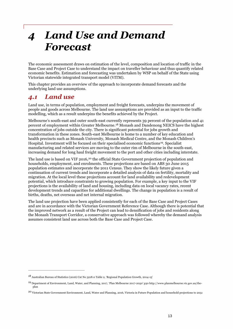
4.1 Land use Land use, in terms of population, employment and freight forecasts, underpins the movement of people and goods across Melbourne. The land use assumptions are provided as an input to the traffic modelling, which as a result underpins the benefits achieved by the Project.
Melbourne’s south-east and outer south-east currently represents 39 percent of the population and 41 percent of employment within Greater Melbourne.18 Monash and Dandenong NEICS have the highest concentration of jobs outside the city. There is significant potential for jobs growth and transformation in these zones. South-east Melbourne is home to a number of key education and health precincts such as Monash University, Monash Medical Centre, and the Monash Children’s Hospital. Investment will be focused on their specialised economic functions19. Specialist manufacturing and related services are moving to the outer rim of Melbourne in the south-east, increasing demand for long haul freight movement to the port and other cities including interstate.
The land use is based on VIF 2016,20 the official State Government projection of population and households, employment, and enrolments. These projections are based on ABS 30 June 2015 population estimates and incorporate the 2011 Census. They show the likely future given a continuation of current trends and incorporate a detailed analysis of data on fertility, mortality and migration. At the local level these projections account for land availability and redevelopment potential, which introduce constraints to growing population. For example, a key input to the VIF projections is the availability of land and housing, including data on local vacancy rates, recent development trends and capacities for additional dwellings. The change in population is a result of births, deaths, net overseas and net internal migration.
The land use projection have been applied consistently for each of the Base Case and Project Cases and are in accordance with the Victorian Government Reference Case. Although there is potential that the improved network as a result of the Project can lead to densification of jobs and residents along the Monash Transport Corridor, a conservative approach was followed whereby the demand analysis assumes consistent land use across both the Base Case and Project Case.
18 Australian Bureau of Statistics (2016) Cat No 3218.0 Table 2, ‘Regional Population Growth, 2014-15’
19 Department of Environment, Land, Water, and Planning, 2017, ‘Plan Melbourne 2017-2050’ p30 http://www.planmelbourne.vic.gov.au/the-
plan
20 Victorian State Government Environment, Land, Water and Planning, 2016, Victoria in Future Population and household projections to 2051

VicRoads PwC 14
Figure 4: Melbourne’s land use
Source: WSP, Victoria in Future 2016 https://www.planning.vic.gov.au/land-use-and-population-research/victoria-in-future-2016
VIF 2016 forecast21 the population of Melbourne to grow from 5.1 million in 2021 to 6.0 million in 2031, a compounded annual growth rate of 1.7%. From 2031, the population then grows at 1.4 percent to 8 million in 2051. As shown in Figure 4, the South – east contributes significantly to this growth. In Melbourne’s south-east and outer south-east, Cardinia and Casey is expected to have the highest population growth of 3.2 percent and 2.3 percent respectively, resulting in 0.16 million and 0.44 million total residents by 2031. Similarly population in other region in the south-east such as Dandenong, Frankston and Glen Eira are expected to grow at 1.3 percent, 0.9 percent and 0.9 percent respectively by 2031. During this time population in Boroondara, Knox, Manningham, Monash, Whitehorse and Yarra Ranges located in the Melbourne’s east and south-east are expected to grow at compounded annual growth rate of 0.9 percent from 1.1 million to 1.2 million in 2031.
4.2 Role of demand forecasts in the economic assessment
4.2.1 Key elements of traffic modelling for economic assessment The traffic modelling that underpins the economic appraisal is undertaken by WSP, using the Victorian Integrated Transport Model developed and maintained by Transport for Victoria (TFV).
The VITM is the standard strategic modelling tool for transport planning investigations in Victoria. This model is a multimodal four-step strategic transport model that uses future population and employment projections to forecast the future impacts of changes to the Melbourne road and public transport networks. The model is therefore a powerful strategic planning tool used by TfV and VicRoads to assist in the planning of road and public transport infrastructure for Victoria, particularly
21 Department of Environment, Land, Water, and Planning, 2017, Victoria in Future Population and household projections to 2051
Population in Melbourne 2016
Population change in Melbourne 2016 to 2031
Employment in Melbourne 2016
Employment change in Melbourne 2016 to 2031

VicRoads PwC 15
for comparing the likely impacts of scenarios under different transport network assumptions. The VITM is therefore a suitable tool for this Project as it requires transport modelling at the strategic level to inform assessment of different road network options.
The most relevant aspects of WSP’s demand modelling for estimating economic benefits are:
Forecasts of total travel demand (across all transport modes) are estimated by VITM for 2020/21, 2030/31 and 2050/51 based upon relationships between demand and the location of activities. Forecasts of the transport network as well as employment and population numbers/locations are key inputs into the VITM model that drive underlying demand for trips. The CBA draws on traffic outputs in these years with extrapolation/interpolation between and following those years in order to develop forecasts of economic benefits.
Demand is modelled across four time periods within a representative weekday (AM peak 7-9AM, inter-peak 9AM-3PM, PM peak 3-6PM and off-peak 6PM-7AM periods) with trip choices constraining choices within a day (e.g. if a user takes public transport to work, they cannot drive home later that night). This is relevant as the CBA should reflect variances across the day and not only during peak periods. The mix of vehicles, trip purposes and levels of congestion will also change throughout the day, impacting both demand outputs and unit cost parameters used to estimate economic benefits.
Vehicle type is modelled per trip – car, commercial vehicles and public transport costs are weighed up by travellers. The CBA is therefore able to measure benefits by vehicle type, reflecting that values of time and vehicle operating costs vary by type of vehicle.
The transport network’s characteristics determine the extent to which demand feeds back into and alters transport costs, e.g. high demand for a road will result in slower travel times (congestion), which will tend to dampen demand for the road (prompting users to switch routes or travel modes). The model seeks to find the equilibrium between routes, modes and destinations such that future travel demand is distributed across the transport network in a realistic fashion.
The model captures multiple sources of induced demand/traveller behaviour in relation to changes in route, mode and destinations. The VITM modelling of travel behaviours assumes users can change modes, routes and destinations in response to changes in the transport network. Total trip numbers between a given origin and destination are not necessarily the same in the Base Case and Project Case.
Table 6: Types of induced demand available in VITM model in response to road improvement
Type Description Incorporated in the VITM model
Changing route Drivers make the same journeys but use the improved route Yes
Changing destination
Drivers decide to travel to more distant destinations because the improvement makes the journey time acceptable
Yes
Changing mode Public transport passengers switch to car because the improvement makes road travel more attractive than rail
Yes
Changing time of travel
Drivers decide to travel in the commuting peak period because the improvement reduces journey times to an acceptable level
No
Making additional journeys
People are willing to make additional car journeys because of the improvement No
Relocated trips People and businesses relocate to take advantage of the improvement and so make journeys that are new to the area
No
Source: Victorian Auditor General, 2011, Management of Major Road Projects, page 8
The VITM was validated using a two-stage process:

VicRoads PwC 16
Network wide validation is based on Melbourne Metro VITM model for base year 2011. It
includes highway screen lines, public transport boarding and mode split.
Project specific validation is for the 2016 forecast. It included traffic volumes validation on
Monash Freeway and arterial roads in the south-east, travel time/speed validation along
Monash Freeway.
4.2.2 Raw demand forecasts The VITM estimates network demand in Melbourne (Base Case) to grow from 86 million car Vehicle Kilometres Travelled (VKT) in 2021 to 99 million in 2031 and then at a Compounded Annual Growth Rate (CAGR) of 1.8 percent to 119 million in 2051.22 With the Monash Freeway upgrades the modelling results show similar trends with a slight increase in overall demand. However, the project results in significant travel time savings for users particularly in the AM peak period (more detail is provided in Section 6.2.1. These benefits result from an improvement in volume capacity ratios derived from the Project.
The modelling indicates that the major beneficiaries of the Project are existing road users. As shown in Figure 5 travel time savings for existing users are 128 million minutes in 2021 and grow to 369 million minutes in 2051 while the new user travel time savings are much lower at 7 million minutes in 2021 and grow to 15 million minutes in 2051.
Figure 5: Travel Time Savings in Project Case compared to Base Case (average day)
Source: PwC, 2017 visualisation, WSP modelling results using Victorian Integrated Transport Model (VITM), Base case and Bundle 3 2021, 2031, 2051 (2017)
The modelling results also indicate that more users travel at higher speeds. Figure 6 shows that compared to the Base Case more commuters travel at speeds greater than 70km/hr and there is significant reduction in travel at speed less than 30km/hr. This reduction in travel at lower speeds results in vehicle operating cost savings.
Figure 6: Kilometres travelled by speed in Project Case compared to Base Case (average day)
Source: PwC, 2017 visualisation, WSP modelling results using Victorian Integrated Transport Model (VITM), Base Case and Bundle 3- 2021, 2031, 2051 (2017)
22 PwC analysis, WSP modelling results using Victorian Integrated Transport Model (VITM), Base case - 2021, 2031, 2051 (2017)
15
17
7
369
278
128
0 50 100 150 200 250 300 350 400
2051
2031
2021
Million minutes
Existing New
Existing users gain maximum benefits
-400
-200
-
200
400
10 30 50 70 90 90+
Kilo
metr
es ('000)
Speed (km/hr)
Increased travel at higher speeds

VicRoads PwC 17
4.3 Incorporating demand forecasts Two adjustments are made to 2020/21, 2030/31 and 2050/51 transport demand outputs to deliver a complete and realistic profile of impacts (and hence benefits) over the economic appraisal period. These adjustments fill in gaps between the available forecast years as well as scale the modelled (‘steady state’) impacts according to how long real-world travellers will take to change their behaviours.23 They include annualisation and interpolation/extrapolation. Recognising that existing users gain majority of the project benefits, project demand is assumed to occur at opening of the project and hence no steady ramp-up of benefits was applied.
4.3.1 Annualisation An annualisation factor of 320 was applied to derive annual benefits from average weekday VITM outputs. As no specific guidance on road annualisation factors is available in the IA 2017 Guidelines, ATAP 2016 Guidelines or Vic DTF 2013 HVHR guidelines, it was necessary to examine traffic statistics for weekdays versus weekends on Melbourne’s road network. This aligned with Victorian Transport Guidelines which state that the specific characteristics of the network in which the project is assessed be considered24
The annualisation factor was calculated at four key points on Monash Freeway based on actual traffic volumes observed East of Warrigal Road, East of Huntingdale Road, East of Springvale Road and East of EastLink. Comparing average traffic volumes on a school term weekday to annual traffic volumes at these road intersections with the Monash Freeway indicate the annualisation factor should range from 321-336 (see Table 7). However to be conservative, the analysis applies 320 as an annualistion factor. Similarly this number is conservative when comparing annualisation factors calculated on surrounding arterial road which are higher than 320 (344 at Oshea Road / Greaves Road / Clyde Road, 328 at Westall Road / Princes Highway, 328 at Springvale Road / Wellington Road) with the exception of Blackburn Road / Wellington Road which is slightly lower at 315 (see Table 8).
Table 7: Traffic volumes – Monash Freeway
Weekday Traffic Volume*
(A)
Annual Traffic Volume
(T)
Annualisation
Factor
(T/A)
East of Warrigal Road 192,812 62,039,632 321
East of Huntingdale Road 207,609 69,357,180 334
East of Springvale Road 182,817 61,537,540 336
East of Eastlink 161,719 54,042,809 334
Note* Represents Average School Term Weekday Traffic Volumes Source: VicRoads, 2017 calculations based on average of days in 2016.
23 Experience has shown that it takes time for transport users to adjust to the changed transport conditions on the network, especially the
improved travel times offered by the new infrastructure. In contrast, transport demand models are based on all information about the network being incorporated instantly by transport users.
24 DEDJTR Guidelines for Transport Modelling and Economic Appraisal in Victoria (v3.03 May 2017)
VicRoads PwC 18
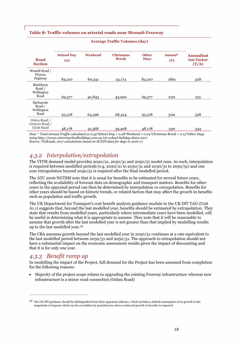
Table 8: Traffic volumes on arterial roads near Monash Freeway
Road Section
Average Traffic Volumes (day)
Annualisation Factor
(T/A)
School Day
(A)
Weekend
Christmas Break
Other Days
Annual^
(T)
Westall Road / Princes
Highway 84,210 60,341 54,174 84,210 28m 328
Blackburn Road /
Wellington Road 69,577 40,843 43,920 69,577 21m 315
Springvale Road /
Wellington Road 93,318 64,396 68,424 93,318 31m 328
Oshea Road / Greaves Road /
Clyde Road 48,178 41,368 39,408 48,178 13m 344
Note ^ Total Annual Traffic calculated as 0.55*School Day + 0.28*Weekend + 0.04*Christmas Break + 0.13*Other Days using http://www.victoriaschoolholidays.com.au/vic-school-holiday-dates-2017 Source: VicRoads, 2017 calculations based on SCATS data for days in 2016-17.
4.3.2 Interpolation/extrapolation The VITM demand model provides 2020/21, 2030/31 and 2050/51 model runs. As such, interpolation is required between modelled periods (e.g. 2020/21 to 2030/31 and 2030/31 to 2050/51) and one year extrapolation beyond 2050/51 is required after the final modelled period.
The ATC 2006 NGTSM note that it is usual for benefits to be estimated for several future years, reflecting the availability of forecast data on demographic and transport matters. Benefits for other years in the appraisal period can then be determined by interpolation or extrapolation. Benefits for other years should be based on historic trends, or related factors that may affect the growth in benefits such as population and traffic growth.
The UK Department for Transport’s cost benefit analysis guidance module in the UK DfT TAG (Unit A1.1) suggests that, beyond the last modelled year, benefits should be estimated by extrapolation. They state that results from modelled years, particularly where intermediate years have been modelled, will be useful in determining what it is appropriate to assume. They note that it will be reasonable to assume that growth after the last modelled year is not greater than that implied by modelling results up to the last modelled year.25
The CBA assumes growth beyond the last modelled year in 2050/51 continues at a rate equivalent to the last modelled period between 2030/31 and 2050/51. The approach to extrapolation should not have a substantial impact on the economic assessment results given the impact of discounting and that it is for only one year.
4.3.3 Benefit ramp up In modelling the impact of the Project, full demand for the Project has been assumed from completion for the following reasons:
Majority of the project scope relates to upgrading the existing Freeway infrastructure whereas new
infrastructure is a minor road connection (Oshea Road)
25 The UK DfT guidance should be distinguished from their appraisal software, which includes a default assumption of no growth in the
magnitude of impacts which can be overridden by practitioners where continued growth in benefits is expected.

VicRoads PwC 19
The demand modelling indicates that majority of users of the new infrastructure will be existing
users of the Freeway. This is evident in the time savings from the Project with existing users
gaining 94% of the benefits.
With only minor induced demand (coming from new users), the impact of ramp up will be minor
as there will only be limited change in overall travel behaviour expected
The above assumption is consistent with the standard approach in the DEDJTR 2016 guidelines which assumes that full demand will occur at Project opening.

VicRoads PwC 20
5 Costs
Capital costs associated with construction, ongoing operations and maintenance of the Project are incorporated in the economic assessment as a comparative point to the economic benefits in the CBA.
This chapter provides an overview of the financial costs detailed in attachment D – Cost Estimate Report and documents the steps followed to incorporate in the CBA methodology.
5.1 Capital, operating and maintenance estimates Capital costs have been included during construction of the project (2019/20-2021/22) and ongoing operating and maintenance costs have been included from the first year of operations (2022/23) to the end of the appraisal period. Capital costs include state management, statutory planning and land acquisition costs
The key components of the cost estimate are:
Direct and indirect costs estimated by Aquenta based on preliminary designs prepared by
VicRoads and its technical adviser. The cost allowance includes provision for State
management and procurement costs
Land acquisition costs estimated based on advice from the Victorian Valuer-General
A P50 risk adjustment that includes both inherent and contingent risk adjustments. Inherent risks include “business as usual” risks such as differences in forecasts of prices and quantities expected to occur during Project delivery. Contingent risks are those risks that arise if the assumptions that form the basis of the capital cost estimate do not prove to be valid or constant, or if there are events that were not foreseen and accounted for in the estimate.
5.2 Economic cost adjustments Nominal costs were adjusted for inclusion in the economic appraisal by incorporating only real escalation in excess of the inflation rate. The nominal costs (P50) were first converted to real (June 2016) dollars and then adjusted for real escalation based on the department’s annual schedule of escalation parameters and adjusted using the mid-point of the Reserve Bank of Australia (RBA) inflation target range 2.5 percent.26
Table 9: Capital Cost ($ million)
Bundle 3A Bundle 3B
Nominal undiscounted (P90) 711 600
Nominal undiscounted (P50) 663 553
Real undiscounted 615 512
Real discounted* 498 415
Note* includes above real escalation Source: PwC, 2017 and Aquenta 2017
26 DEDJTR Guidelines for Transport Modelling and Economic Appraisal in Victoria (v3.03 May 2017)

VicRoads PwC 21
6 Benefits
The Project will generate a number of benefits for road users, the Melbourne community and the economy more broadly. The benefits quantified and monetised in the CBA include direct economic benefits for Victoria. This chapter identifies each benefit assessed and outlines the methodology applied to estimate each.
6.1 Benefits of the Project The Project will provide a number of benefits for Melbourne transport users and for the city’s economy more broadly. These will be as a result of improvements in transport network efficiency and congestion for road users, improved efficiency of freight movement, greater resilience and redundancy in the transport network, a more liveable Melbourne, and improved connectivity and economic development in Melbourne. The key benefits identified and incorporated into the CBA are outlined in Table 10.
Table 10: Economic benefits of the Project
Overarching benefits Benefit category captured in economic assessment
Productivity and growth for Melbourne
Travel time savings from improved traffic flow – cars
Vehicle operating cost savings – cars
Travel time savings from improved reliability – cars
Perceived travel time savings from reduced congestion – cars
Resilience to lane closures on the Monash Freeway
Travel time savings from improved traffic flow – LCV and HCV*
Vehicle operating cost savings – LCV and HCV*
Travel time savings from improved reliability – LCV and HCV*
Safety and environment benefits
Crash cost savings
Environmental benefits
Economy-wide benefits Agglomeration
Imperfect competition
Macroeconomic development in the State and nationwide
Note* :light commercial vehicles(LCV) and heavy commercial vehicles(HCV) together represent commercial vehicles for freight Source: PwC, 2017
The approach to estimating each of the identified economic benefit categories has been based on welfare economic theory, whereby the change in economic value measured is defined by changes in travel conditions in terms of the theoretical concepts listed below:
User benefits – the change in value that is perceived by users of the affected transport services. The change in ‘consumer surplus’27 is comprised of effects on:
27 This appraisal approximates the change in consumer surplus as changes in generalised trip cost (GTC), the measure of the perceived cost of
travel.
VicRoads PwC 22
a. Existing transport users – change in perceived costs of existing road and public transport users (‘transport users’) who do not change behaviour with the project, and
b. New and lost transport users – change in perceived cost of transport users who change their behaviour (different mode or destination compared to the base case).
Resource cost corrections – the opportunity costs of resources expended by undertaking and/or supplying a transport trip, measured from a societal perspective (since the perceived cost of travel as described above does not always reflect the associated change in resource costs). Examples include the cost of tyres, depreciation, insurance and public transport fares.28 Differences between perceived and resource costs arise due to gaps in information, misperceptions, taxes, subsidies and financial transfers
Externalities – effects on other transport system users and non-users. Externalities are measured as the difference between social resource costs and private resource costs. Examples of such externality effects include congestion, road crashes, amenity and environmental effects
Network resilience benefit – Melbourne’s south - east and outer south-east is heavily reliant on the Monash Freeway to access the city and surrounding areas along the corridor. An unplanned lane closure on the Monash Freeway can cause significant delays across the entire transport corridor. Improving capacity in the Corridor will help the Monash Freeway and the broader network be more resilient such that it is better able to handle unplanned incidents and other stop-start conditions
Wider economic benefits – improvements in national output that are not already reflected in user travel costs elsewhere in the appraisal. Agglomeration benefits are one example, as these reflect the benefits collectively experienced by clusters of businesses being brought closer together (in terms of shorter travel times).
The remainder of this chapter documents the detailed methodology applied to quantify above benefits for the Project. It is worth noting, that the above list is not comprehensive as there are additional benefits from the Project not quantified in the CBA. For example:
The Project is expected to generate macroeconomic activity induced through increased expenditure
during construction. During the construction phase GSP and employment will spike while post
construction, productivity improvements associated with the Project will continue to increase
employment and activity
The Project is expected to foster urban renewal and unlock development potential in Melbourne’s east and outer south-east. Urban renewal benefits such second round transport benefits, second round wider economic benefits, avoidable costs, and land value uplift if captured will potentially result in a higher BCR
The Project scope includes upgrades to public transport and active transport infrastructure such as new shared paths and relocating/building new bus stops. The benefits to the public transport users and active transport users as a result of these upgrades have not been quantified.
6.2 User benefits Road users of the Melbourne transport network and in particular the Monash Freeway will be key beneficiaries of the Project. The freeway widening and interchange works at Beaconsfield and Oshea Road will improve transport network efficiency and congestion for road users by providing better connectivity along Melbourne’s south-east and outer south-east corridor.
The user benefits estimated are related primarily to savings in transport user costs due to a reduction in travel times and distances compared with the Base Case:
Travel time savings
28 ATC, 2006, National Guidelines for Transport System Management in Australia, Volume 3, p 58.

VicRoads PwC 23
Reliability benefits
Savings in vehicle operating costs
Perceived congestion benefits
Applying VITM demand model outputs based on consumer surplus theory
The structure of the traffic demand forecasting model determines how the change in consumer surplus is estimated for the purposes of economic analysis. Traffic and demand modelling has been based on variable trip matrix methods that recognise that transport is an intermediate service used to access activities which generate value. Travellers will seek to maximise the net benefit of travel, rather than simply minimise cost and therefore may choose to access more distant destinations if the costs of reaching them decline. In short, there may be any number of behavioural (induced) changes which occur as a result of the project, including travellers changing their mode or their destinations by travelling further.
The simple supply/demand representation is generalised below to identify the change in consumer surplus when these demand changes are captured. The key aspect of this figure is that the number of trips by mode m (e.g. private vehicle) between ij increase to TProject with the Project. Accordingly, the consumer surplus increases from those confined to existing users to include the ‘triangle’ associated with the net benefit enjoyed by the switching users (Figure 7).
Figure 7: Change in consumer surplus with variable trip matrices
Source: PwC, 2017
The total net benefit in the figure above can be explained in terms of the two segments of demand following the introduction of the Project for a particular ij:
Each existing user willing to pay Generalised Cost (GC) GCBase Case given by the intersection of the trip supply and demand curve in the base case but pays only GCProject with the Project. This results in an increase in net benefit of GCBase Case - GCProject for each existing user.
The net benefit enjoyed by switching users (mode or destination switchers) is given by the pink triangle. By definition, switchers were not willing to pay GCBase Case to travel between ij by mode m (otherwise they would have travelled with the base case and comprise an existing user); however, they are prepared to pay at least GCProject. The first new user who switched to ij by mode m would have been willing to pay a price which is slightly less than GCBase Case. Therefore, the net benefit for the user would be slightly below the benefits enjoyed by existing users, i.e. GCBase Case - GCProject. The last few people who decide to switch to ij by mode m would only be willing to pay slightly less than the new trip cost, i.e. GCProject and hence, their net benefit from switching is effectively zero. Therefore, the average increase in net benefit for the switchers is between slightly above zero and

VicRoads PwC 24
slightly less than GCBase Case - GCProject. Therefore, on average, the net benefit to a switcher is 0.5*(GCBase Case - GCProject), i.e. the benefit enjoyed by each switcher is on average half the benefit attained by existing users on that ij. This is commonly known as the ‘rule of half’.
Those who change trip behaviour (mode or destination switchers) are new with respect to their newly chosen alternative and lost with respect to previously chosen alternative. The calculation of the net benefit enjoyed by existing users remains unchanged. However, by introducing the ability for travellers to choose across a range of trip elements means that the method used to calculate net benefit of induced users must be generalised. This is done by first defining new, lost and existing trips (T) as follows:
continuing users of a mode/destinationij =min (TBase Case, TProject)
new tripsij = max(TProject - TBase Case, 0)
lost tripsij = max(TBase Case - TProject Case, 0)
The second step to estimating consumer surplus is to apply the incremental Generalised Travel Cost (GTC) between the base case and the project case, i.e.
continuing user benefits = (GCBase Case - GCProject) * min (TBase Case, TProject)
new user benefits = (GCBase Case - GCProject) * max (TProject - TBase Case,0) * 0.5
lost user benefits = (GCBase Case - GCProject) * max(TBase Case - TProject Case, 0) * 0.5
These calculations are applied in VITM for each time period, travel mode and vehicle class, and then aggregated across each ij pair before being reported to PwC for each component of GTC such as travel time, vehicle operating cost etc.
The following sub-sections describe the methodologies for estimating each individual component of the generalised travel time benefits in a given forecast year.
6.2.1 Travel time savings The Project is expected to reduce congestion and result in significant travel time savings. Figure 8 and Figure 9 show that trips originating around Dandenong and Pakenham gain the most travel time savings. As an example, in 2031, AM peak travel time from Pakenham to Hawthorn/Malvern will be a total of 76 minutes, being 9 minutes quicker than in the Base Case of 85 minutes. In the PM peak period travel time between these zones in the reverse direction will be 13 minutes quicker (the difference between 79 minutes in the Project Case and 92 minutes in the Base Case29). Average speeds for these journeys will be 37 km/hr compared to 32 km/hr in the Base Case, 12 percent faster in the morning peak. In the afternoon peak, average speed will be 17 percent faster in the Project Case compared to Base Case.30
29 Travel time provided by WSP using VITM travel zone 2424 (Pakenham) and 1555 (inner east)
30 Travel speeds provided by WSP using VITM travel zone 2424 (Pakenham) and 1555 (inner east)

VicRoads PwC 25
Figure 8: Travel Time Benefits by Origin – Car, AM Peak (7am - 9am), 2031
Source: WSP modelling results using Victorian Integrated Transport Model (VITM), 2031 Bundle 3 (2017)
Figure 9: Travel Time Benefits by Destination – Car, AM Peak (7am - 9am), 2031
Source: WSP modelling results using Victorian Integrated Transport Model (VITM), 2031 Bundle 3 (2017)
Upgrading the Monash Freeway will reduce travel time of freight moving through the Corridor. This would have positive flow on effects for businesses and institutions in the area that need to deliver goods frequently as part of their daily activities. As a result the service sector would be a significant beneficiary from these freight travel time savings. Figure 10 indicates that the benefits to commercial vehicles trips by origin are dispersed whereas Figure 11 indicates that the benefits to these trips are clustered around Monash as a destination zone.

VicRoads PwC 26
Figure 10: Travel Time Benefits by Origin – Commercial Vehicle, Day, 2031
Source: WSP modelling results for LCV and HCV using Victorian Integrated Transport Model (VITM), 2031 Bundle 3 (2017)
Figure 11: Travel Time Benefits by Destination – Commercial Vehicle, Day, 2031
Source: WSP modelling results for LCV and HCV using Victorian Integrated Transport Model (VITM), 2031 Bundle 3 (2017)
Calculation approach based on VITM demand model outputs
For the purpose of economic quantification, improvements in base travel times are assumed to accrue in the form of consumer surplus to:

VicRoads PwC 27
existing road users who divert to the Project or take advantage of reduced congestion
travellers switching modes of transport due to the improved travel times offered by the Project
travellers switching their origins and/or destinations to access more desirable destinations (which may involve taking longer trips)
Savings in base travel times for the project case have been estimated relative to the base case for existing users and switchers, with the latter estimated based on new and lost user calculations.
The demand model has been specified to estimate the travel time component of generalised trip cost (GTC) savings in terms of person hours for car users (by applying estimates of vehicle occupancies across journey purposes) and public transport users, and in terms of vehicle hours for commercial vehicles.
Approach to monetise
Following the estimation of travel time savings by vehicle type for the Base Case and Project Case, monetisation of travel time benefit involved applying the relevant value of travel time for each of the following four broad user types:
Car (business) – for business purposes, time spent on trips made for business purpose (work travel from, or returning to, the workplace, but excluding commuting) is directly valued by employers at the direct resource cost i.e. the average wage rate. Time spent driving in congested conditions is also perceived as a cost valued at travellers’ average willingness to pay to avoid congested conditions.
Car (non-business) – for non-business journey purposes, time is valued according to travellers’ average willingness to pay for additional leisure time and to avoid travelling in congested conditions.
Commercial vehicles (light and heavy) – these business purpose journeys are also valued at the average wage rates (which can vary by the specific vehicle class). In addition, the freight carried by the vehicles also has an opportunity cost from sitting in traffic. Vehicle classes with greater average freight loads are estimated to have greater values of freight time.
Public transport– passenger journeys are valued according to travellers’ average willingness to pay for additional leisure time while driver time is valued at the average wage rate.
Car (business) and car (non-business) base travel time savings can be valued directly by applying the ATAP 2016 Guidelines to the VITM demand modelling outputs (travel time saving hours). For commercial vehicles a weighted average value of time is required. WSP supplied PwC with VicRoads estimates of 2016 Monash Freeway traffic counts across Austroads vehicle categories. These proportions were applied to the ATAP31 estimates of driver and freight values of time for each class to derive the weighted values of travel time.
The data and parameters used in the valuation of time saving benefits are shown in Table 11.
Table 11: Estimation of base travel time savings for improved traffic flow
Element Input
Data Travel time saving hours (project case versus base case) from the demand model, broken down into:
User types – heavy vehicles, car (business), car (non-business), commercial vehicle and public transport
Time periods – AM Peak, PM Peak, Inter-Peak and Off-Peak.
31 Transport and Infrastructure Council, 2016, Australian Transport Assessment and Planning Guidelines, Road Parameter Value

VicRoads PwC 28
Parameters Unit value of travel time savings (VOTT) (values below are in June 2017 dollars, using ABS’s Victorian Wage Price Index). Australian Transport Assessment and Planning 2016 Road Parameter Values are broken down into user types, with HCV values weighted to reflect Melbourne 2016 vehicle composition on the Monash Freeway.
car (business) = $53.58/hr (resource cost of employee time)
car (non-business) = $16.52/hr (willingness to pay for leisure time)
commercial vehicles (LCV and HCV)= $49.58/hr (wage + freight)
Public transport value of travel time = $14.01/hr (willingness to pay for leisure time).
Calculation (simplified32) 𝑇𝑖𝑚𝑒 𝑠𝑎𝑣𝑖𝑛𝑔 𝑏𝑒𝑛𝑒𝑓𝑖𝑡 = ∑ 𝑇𝑖𝑚𝑒 𝑠𝑎𝑣𝑖𝑛𝑔𝑢𝑠𝑒𝑟 𝑡𝑦𝑝𝑒 ∗ 𝑉𝑂𝑇𝑇𝑢𝑠𝑒𝑟 𝑡𝑦𝑝𝑒
𝑢𝑠𝑒𝑟 𝑡𝑦𝑝𝑒
These time saving benefits are calculated for each of the modelled time periods and are then scaled to annual values using the annualisation factor to reach an annual value for the forecast year.
Source: PwC, 2017 2017
6.2.2 Reliability benefits Reliability can be defined as unpredictable or random variation in journey times. This covers variability in the degree of congestion during the same period each day (e.g. random variability) and incidents. This definition excludes predictable variation associated with regular peaks in demand during particular the times of day, days of week, and seasons (e.g. school holidays) which travellers are assumed to be able to predict.33
The Project is expected to reduce the travel time variability for trips in Melbourne’s south-east and outer south-east. Commuters, businesses and other travellers will be able to plan the time for their journey with more certainty. This means that some travellers will be able to reduce the travel time buffer allowance (the extra time travellers allow to make sure they will reach their destination on time). For example, travel time variability between the two zones directly adjacent to the upgraded Monash Freeway section between Cardinia Road and Clyde Road can reduce by 7 minutes.34
32 Two major extensions were applied in practice: (1) the use of the rule of half for time savings for new and lost users; (2) for public transport
users, ‘time savings’ are actually ‘generalised travel cost’ (GTC) savings. GTC measures the perceived cost of travel, including higher perceived costs of a minute of travel time spent waiting at bus or tram stops compared with a minute spent in vehicle.
33 UK Department for Transport, The Reliability Sub-Objective, TAG Unit 3.5.7, April 2009
34 WSP calculation based on trips between zone 2425 to 2048 travelling outbound in PM peak period.
VicRoads PwC 29
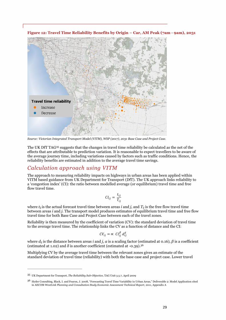
Figure 12: Travel Time Reliability Benefits by Origin – Car, AM Peak (7am - 9am), 2031
Source: Victorian Integrated Transport Model (VITM), WSP (2017), 2031 Base Case and Project Case.
The UK DfT TAG35 suggests that the changes in travel time reliability be calculated as the net of the effects that are attributable to prediction variation. It is reasonable to expect travellers to be aware of the average journey time, including variations caused by factors such as traffic conditions. Hence, the reliability benefits are estimated in addition to the average travel time savings.
Calculation approach using VITM
The approach to measuring reliability impacts on highways in urban areas has been applied within VITM based guidance from UK Department for Transport (DfT). The UK approach links reliability to a ‘congestion index’ (CI): the ratio between modelled average (or equilibrium) travel time and free flow travel time.
𝐶𝐼𝑖𝑗 = 𝑡𝑖𝑗
𝑇𝑖𝑗
where tij is the actual forecast travel time between areas i and j, and Tij is the free flow travel time between areas i and j. The transport model produces estimates of equilibrium travel time and free flow travel time for both Base Case and Project Case between each of the travel zones.
Reliability is then measured by the coefficient of variation (CV): the standard deviation of travel time to the average travel time. The relationship links the CV as a function of distance and the CI:
𝐶𝑉𝑖𝑗 = ∝ 𝐶𝐼𝑖𝑗𝛽 𝑑𝑖𝑗
𝛿
where dij is the distance between areas i and j, α is a scaling factor (estimated at 0.16), β is a coefficient (estimated at 1.02) and δ is another coefficient (estimated at -0.39).36
Multiplying CV by the average travel time between the relevant zones gives an estimate of the standard deviation of travel time (reliability) with both the base case and project case. Lower travel
35 UK Department for Transport, The Reliability Sub-Objective, TAG Unit 3.5.7, April 2009
36 Hyder Consulting, Black, I. and Fearon, J. 2008, “Forecasting Travel Time Variability in Urban Areas,” Deliverable 2: Model Application cited
in AECOM WestLink Planning and Consultation Study Economic Assessment Technical Report, 2011, Appendix A

VicRoads PwC 30
times with the project are associated with reductions in the standard deviation of average journey times.
𝐴𝑣𝑒𝑟𝑎𝑔𝑒 𝑠𝑡𝑎𝑛𝑑𝑎𝑟𝑑 𝑑𝑒𝑣𝑖𝑎𝑡𝑖𝑜𝑛 𝑐ℎ𝑎𝑛𝑔𝑒 (ℎ𝑟𝑠) = ∑𝑇𝑟𝑖𝑝𝑠𝑖𝑗 ∗ ∆( 𝑡𝑖𝑗 ∗ 𝐶𝑉𝑖𝑗
𝑖,𝑗
)
= ∑𝑇𝑟𝑖𝑝𝑠𝑖𝑗 ∗ ∆( 𝑡𝑖𝑗 ∗
𝑖,𝑗
0.16 (𝑡𝑖𝑗
𝑇𝑖𝑗)
1.02
𝑑𝑖𝑗−0.39)
where Tripsij is the number of trips between areas i and j.
Approach to monetise
Valuation of the change in reliability is via the ‘reliability ratio’, i.e. the value of a saved hour of standard deviation of travel time relative to the value of a saved hour of average travel time. Hyder suggests a value of 0.8 for light vehicles and 1.2 for heavy vehicles.37 The data and parameters used in the calculation of reliability benefits are shown Table 12 .
Table 12: Estimation of reliability benefits
Element Input
Data Average standard deviation reduction (project versus base case) from the demand model and subsequent calculations, broken down into:
Time periods – AM Peak, PM Peak, Inter-Peak and Off-Peak
Origins and destinations (O-D) – all modelled O-D pairs
Trip numbers from the demand model, broken down into:
User types – heavy vehicles, car (business) and car (non-business)
Origins and destinations– all modelled O-D pairs
Parameters Reliability ratio by user type were applied to standard deviation within VITM:
– commercial vehicles = 1.2
– car (business) = 1.2
– car (non-business) = 0.8
Calculation 𝑅𝑒𝑙𝑖𝑎𝑏𝑖𝑙𝑖𝑡𝑦 𝑏𝑒𝑛𝑒𝑓𝑖𝑡 = 𝐴𝑣𝑔. 𝑠𝑡. 𝑑𝑒𝑣𝑖𝑎𝑡𝑖𝑜𝑛 𝑟𝑒𝑑𝑢𝑐𝑡𝑖𝑜𝑛 (ℎ𝑜𝑢𝑟𝑠)𝑢𝑥 𝑅𝑒𝑙𝑖𝑎𝑏𝑖𝑙𝑖𝑡𝑦 𝑟𝑎𝑡𝑖𝑜𝑢𝑥 𝑉𝑂𝑇𝑇𝑢
This calculation applies the rule of half to new users and was performed across all vehicle and user types (u) and all travel zones in the transport model. These reliability benefits have been calculated for each of the modelled time periods and provided to PwC in minutes. PwC converted to June 2017 dollars by applying the value of time (𝑉𝑂𝑇𝑇𝑢) in Table 11 and then scaled to annual values using the annualisation factor to reach an annual value for the forecast year.
Source: PwC, 2017 2017
6.2.3 Vehicle operating cost savings In urban conditions such as Melbourne, an improvement in average road travel speeds will be associated with lower vehicle operating costs (VOC) per kilometre for users. In addition, a change in road type or kilometres travelled may also influence the total VOC associated with the Project relative to Base Case.
In making transport decisions users generally consider only some cost (perceived) associated with owning a vehicle such as fuel, car parking, tolls and PT fare savings. This perceived cost generally excludes running costs (fixed and operational) of the vehicle, such as depreciation, repairs and maintenance. However it takes into consideration:
37 Cited in AECOM WestLink Planning and Consultation Study Economic Assessment Technical Report, 2011, Appendix A

VicRoads PwC 31
Additional running costs due to road surface and gradient;
Additional running costs due to any significant speed fluctuations from free flow speed; and
Additional fuel costs due to stopping, such as queuing at traffic signals38
Calculation approach
The calculation approach is based on ATAP 2016 Guidelines which provide VOC equations to estimate the fuel costs associated with travel for 20 vehicle classes (consistent with Austroads vehicle classifications) and for road types freeway (>60 km/hr) and urban/suburban arterial roads (<60 km/hr).39 The equations are based on stop-start and free-flow models and relate average cost per kilometre travelled by a vehicle to the average all day speed on the road.
Stop-start model (for urban arterial): c=A + B/V
Free-flow model (for freeways): c=C0+C1V+C2V2
where, c= vehicle operating cost (cents/km), A, B, C0, C1, C2 = model coefficients, and V= average speed in km/hr.
The stop-start and freeway model parameters applied by VITM are shown in Table 13.
Table 13: Fuel consumption coefficients (litres/100km, June 2013 dollars)
Vehicle Type
Stop – Start Model Free Flow Model
A B C0 C1 C2
Car 8.8017 179.689 9.8014 -0.0785 0.0008
Commercial 45.5089 535.1584 32.0378 -0.2949 0.0040
Note: Commercial Vehicles represent both LCV and HCV Source: Australian Transport Assessment and Planning 2016 Road Parameter Values
In VITM the traffic model outputs (road speeds and vehicle kilometres by vehicle type) were combined with the VOC equations to estimate the VOC in the Base Case and Project Case.40 The other component of perceived cost such car parking and toll were based on the assumptions used in the base transport network for demand modelling. The change in VOC between the base case and option scenarios determines VOC savings associated with the option.
Approach to monetise
The underlying calculations were undertaken in the demand model across all vehicle and all road types. The benefits were calculated for each of the modelled time periods and then scaled to annual values using the annualisation factor to reach an annual value for the forecast year. Table 14 outlines the data, parameters and calculations to estimate the VOC savings.
Table 14: Estimation of vehicle operating cost savings
Element Input
Data Average road speeds from the demand model, broken down into:
Time periods – AM Peak, PM Peak, Inter-Peak and Off-Peak
Road links – all modelled links
Base Case and Project Case
38 RTA, Economic Appraisal Manual, Version 2, Appendix B – Economic Parameters for 2007, pp 4-8.
39 Transport and Infrastructure Council, 2015 National Guidelines for Transport System Management in Australia, p 31-32.
40 These equations are represented directly within VLC’s model.
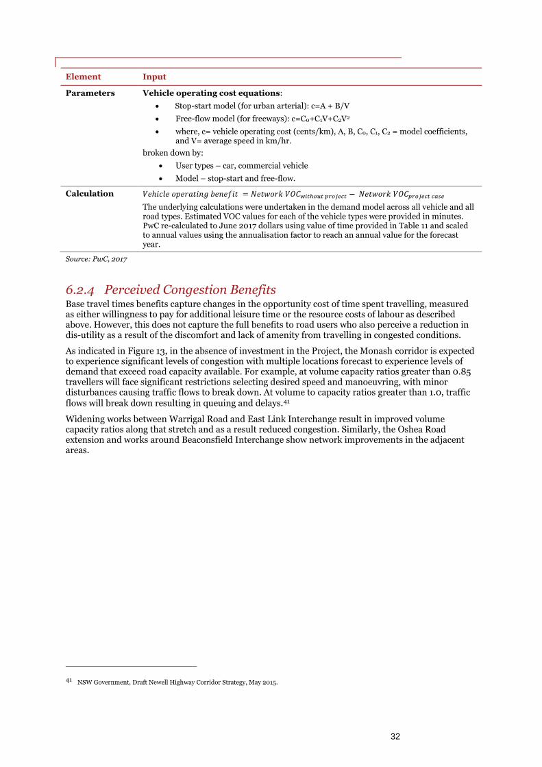
VicRoads PwC 32
Element Input
Parameters Vehicle operating cost equations:
Stop-start model (for urban arterial): c=A + B/V
Free-flow model (for freeways): c=C0+C1V+C2V2
where, c= vehicle operating cost (cents/km), A, B, C0, C1, C2 = model coefficients, and V= average speed in km/hr.
broken down by:
User types – car, commercial vehicle
Model – stop-start and free-flow.
Calculation 𝑉𝑒ℎ𝑖𝑐𝑙𝑒 𝑜𝑝𝑒𝑟𝑎𝑡𝑖𝑛𝑔 𝑏𝑒𝑛𝑒𝑓𝑖𝑡 = 𝑁𝑒𝑡𝑤𝑜𝑟𝑘 𝑉𝑂𝐶𝑤𝑖𝑡ℎ𝑜𝑢𝑡 𝑝𝑟𝑜𝑗𝑒𝑐𝑡 − 𝑁𝑒𝑡𝑤𝑜𝑟𝑘 𝑉𝑂𝐶𝑝𝑟𝑜𝑗𝑒𝑐𝑡 𝑐𝑎𝑠𝑒
The underlying calculations were undertaken in the demand model across all vehicle and all road types. Estimated VOC values for each of the vehicle types were provided in minutes. PwC re-calculated to June 2017 dollars using value of time provided in Table 11 and scaled to annual values using the annualisation factor to reach an annual value for the forecast year.
Source: PwC, 2017
6.2.4 Perceived Congestion Benefits Base travel times benefits capture changes in the opportunity cost of time spent travelling, measured as either willingness to pay for additional leisure time or the resource costs of labour as described above. However, this does not capture the full benefits to road users who also perceive a reduction in dis-utility as a result of the discomfort and lack of amenity from travelling in congested conditions.
As indicated in Figure 13, in the absence of investment in the Project, the Monash corridor is expected to experience significant levels of congestion with multiple locations forecast to experience levels of demand that exceed road capacity available. For example, at volume capacity ratios greater than 0.85 travellers will face significant restrictions selecting desired speed and manoeuvring, with minor disturbances causing traffic flows to break down. At volume to capacity ratios greater than 1.0, traffic flows will break down resulting in queuing and delays.41
Widening works between Warrigal Road and East Link Interchange result in improved volume capacity ratios along that stretch and as a result reduced congestion. Similarly, the Oshea Road extension and works around Beaconsfield Interchange show network improvements in the adjacent areas.
41 NSW Government, Draft Newell Highway Corridor Strategy, May 2015.

VicRoads PwC 33
Figure 13: Volume Capacity Ratio 2031 AM peak (7 – 9 am), Base Case and Project Case
Source: Victorian Integrated Transport Model (VITM), WSP (2017), 2031 Base Case and Project Case
As shown in Figure 14 the reduced congestion as a result of Oshea Road Extension and Beaconsfield Interchange works generates significant travel time savings for trips between Casey and Cardinia. It also improves travel time between Cardinia and Dandenong/Monash employment clusters.
Reduced congestion as a result of Oshea Road Extension and Beaconsfield Interchange works
Reduced congestion as a result of works to widen Freeway
Base Case
Project Case
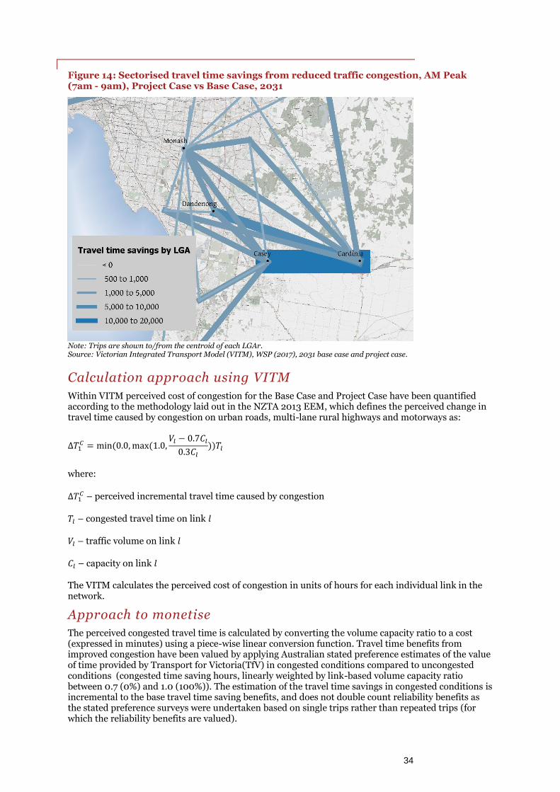
VicRoads PwC 34
Figure 14: Sectorised travel time savings from reduced traffic congestion, AM Peak (7am - 9am), Project Case vs Base Case, 2031
Note: Trips are shown to/from the centroid of each LGAr. Source: Victorian Integrated Transport Model (VITM), WSP (2017), 2031 base case and project case.
Calculation approach using VITM
Within VITM perceived cost of congestion for the Base Case and Project Case have been quantified according to the methodology laid out in the NZTA 2013 EEM, which defines the perceived change in travel time caused by congestion on urban roads, multi-lane rural highways and motorways as:
∆𝑇1𝐶 = min (0.0,max(1.0,
𝑉𝑙 − 0.7𝐶𝑙
0.3𝐶𝑙
))𝑇𝑙
where:
∆𝑇1𝐶 – perceived incremental travel time caused by congestion
𝑇𝑙 – congested travel time on link 𝑙
𝑉𝑙 – traffic volume on link 𝑙
𝐶𝑙 – capacity on link 𝑙
The VITM calculates the perceived cost of congestion in units of hours for each individual link in the network.
Approach to monetise
The perceived congested travel time is calculated by converting the volume capacity ratio to a cost (expressed in minutes) using a piece-wise linear conversion function. Travel time benefits from improved congestion have been valued by applying Australian stated preference estimates of the value of time provided by Transport for Victoria(TfV) in congested conditions compared to uncongested conditions (congested time saving hours, linearly weighted by link-based volume capacity ratio between 0.7 (0%) and 1.0 (100%)). The estimation of the travel time savings in congested conditions is incremental to the base travel time saving benefits, and does not double count reliability benefits as the stated preference surveys were undertaken based on single trips rather than repeated trips (for which the reliability benefits are valued).

VicRoads PwC 35
The data and parameters used in the valuation of time saving benefits are shown in Table 15.
Table 15: Estimation of travel time benefits from reduced traffic congestion
Element Input
Data Travel time saving hours (project case versus base case) from the demand model, broken down by:
User types – car and heavy commercial periods
Parameters Unit value of congested travel time (VoCT) applied in VITM as a proportion to value of time(VoT):
car (business) = 0.11
car (non-business) = 0.34
light commercial vehicles = 0.1 *
heavy commercial vehicles = 0.05*
Calculation (simplified42)
𝐶𝑜𝑛𝑔𝑒𝑠𝑡𝑒𝑑 𝑡𝑖𝑚𝑒 𝑠𝑎𝑣𝑖𝑛𝑔 𝑏𝑒𝑛𝑒𝑓𝑖𝑡
= ∑ 𝐶𝑜𝑛𝑔𝑒𝑠𝑡𝑒𝑑 𝑡𝑖𝑚𝑒 𝑠𝑎𝑣𝑖𝑛𝑔𝑢𝑠𝑒𝑟 𝑡𝑦𝑝𝑒 ∗ 𝑉𝑜𝐶𝑇𝑢𝑠𝑒𝑟 𝑡𝑦𝑝𝑒
𝑢𝑠𝑒𝑟 𝑡𝑦𝑝𝑒
In VITM these congested travel time savings are calculated for each of the vehicle types and converted to minutes. PwC re-calculated to June 2017 dollars using value of time provided in Table 11 and scaled to annual values using the annualisation factor to reach an annual value for the forecast year.
Note*: perceived congestion benefits were aggregated for LCV and HCV and hence the weighted value of time was applied Source: PwC, 2017 and Transport for Victoria Guidelines
6.3 Resource cost corrections The perspective of CBA requires that careful account must be made for actual resources expended and produced. In many cases, private perceptions and valuations of resource flows are the most appropriate method for achieving this accounting and valuation. However, there are several cases where private participants do not adequately perceive actual resource flows with and without the project. A range of resource corrections are therefore required to adjust standard measures of resource savings due to a misalignment of user perceptions versus actual resource use.
In accordance with ATAP 2016 Guidelines, a correction was applied in this CBA to correct for actual resource costs that are borne by or affect travel behaviour changes but are not perceived, and adjustments for transfer payments that are perceived as costs by travellers but do not represent use of any resources.43
Two corrections are required in the CBA to account for the actual flow of resources relative to user perceptions already represented elsewhere: vehicle operating costs and revenue transfer payments.
6.3.1 Vehicle operating cost Car users generally fail or over perceive some of the resource costs they incur. For example, car users will perceive the cost of fuel but may not perceive variable components of vehicle operating cost such as vehicle depreciation, repairs and maintenance and lubricating. A resource correction is thus required to allow for changes in the unperceived resource cost (actual cost) of travel.
Calculation approach
42 Two major extensions were applied in practice: (1) the use of the rule of half for time savings for new and lost users; (2) for public transport
users, ‘time savings’ are actually ‘generalised travel cost’ (GTC) savings. GTC measures the perceived cost of travel, including higher perceived costs of a minute of travel time spent waiting at bus or tram stops compared with a minute spent in vehicle.
43 Transport and Infrastructure Council, Australian Transport Assessment and Planning Guidelines, 2016 M5 Travel behavior Change, pg 15

VicRoads PwC 36
The actual cost was calculated within VITM applying the same methodology as that for perceived VOC as described in Section 6.2.3 using coefficients shown in Table 16.
Table 16: VOC model coefficients for stop-start and free-flow models (litres/100km, June 2013 dollars)
Vehicle Type
Stop – Start Model Free Flow Model
A B C0 C1 C2
Car 12.6514 1315.5178 35.0470 -0.1751 0.0012
Commercial 57.1600 2556.0769 82.2900 -0.5525 0.0053
Note: Commercial vehicles represent both LCV and HCV in VITM Source: Australian Transport Assessment and Planning 2016 Road Parameter Values
Approach to monetise
The difference between the actual and perceived cost were calculated within the VITM for an average weekday for each of the forecast years and provided in minutes. PwC monetised in the CBA by applying value of time provided in Table 11, annualising and inflating to June 2017 prices using ABS Melbourne CPI.
6.3.2 Revenue transfer payments The increase in transport operator revenues stemming from users is ordinarily considered a monetary transfer payment between users and the operator to reflect the resources required to provide the transport services, and hence excluded from CBA. However, from the user’s perspective, tolls and public transport fares are perceived in generalised travel costs when choosing between modes and destinations.44 As the perceived resources are already accounted for (through perceived journey costs in section 6.2.1), there is a need to reflect this additional revenue as a resource correction.
Calculation approach
The resource cost in relation to both tolls and public transport fare should be zero. Thus CBA analysis corrects for the perceived components of this cost by deducting the perceived cost. The difference between the resource cost misperception for the Base Case and Project Case is calculated within VITM as a resource cost correction.
Approach to monetise
Revenue payment transfer corrections are calculated within the VITM for an average weekday for each of the forecast years, and monetised in the CBA by applying an annualisation factor and inflating to $ June 2017 using ABS Melbourne CPI.
6.3.3 Car Parking The resource cost correction for car parking is necessary because the cost contains both unperceived costs and revenue transfers.
Unperceived costs are an adjustment to reflect the fact that in many cases, parking is not being paid by the traveller and as such a correction needs to be applied to reduce the perceived cost of parking. The VITM Economic Module currently assumes that 50% of travellers have their parking paid for, and as such the perceived cost of parking needs to be halved.
44 For example, a project that lowers bus travel times yields direct benefits in generalised travel costs for existing bus users. Importantly, when
the project encourages people to choose to catch a bus instead of driving as previously (i.e. new bus users), it is because in the project case their generalised travel cost is lower by bus than car, even accounting for the travel time and fares. The rule of a half relies on being able to measure the net change in generalised cost from existing bus users as an upper bound estimate of the generalised cost improvement experienced by new bus users. Although the measurement of these existing user benefits is usually based on travel time savings and may not explicitly look at fare component, when new bus user benefits are estimated, the calculated change in generalised trip costs embodies the fare component as the total generalised cost is what is weighed up in the mode choice.
VicRoads PwC 37
Revenue transfers reflect the payment of GST and state levies, and these amounts must be deducted from the parking resource cost.
The resource cost correction is difference between the resource cost and the perceived cost, applied to every traveller which now pays for parking as a result of the project case.
Approach to monetise
Car parking resource cost corrections are calculated within the VITM for an average weekday for each of the forecast years, and monetised in the CBA by applying an annualisation factor and inflating to $ June 2017 using ABS Melbourne CPI.
6.4 Externalities Improving connectivity around the Monash Corridor will translate into an improved quality of life for those living in the east, through improved amenity (e.g. reduced noise, crashes and pollution). A reduction in the number of vehicles moving through residential areas from transferring to the freeway will make communities safer by reducing accidents.
6.4.1 Crash cost savings Crash costs for the Base Case and the Project Case are forecast using crash rates and vehicle trip numbers. The model estimates the number of casualty crashes on each road type (freeway or other roads).
Estimates of the number of crashes are applied to average crash costs by road type in three severity categories: fatal, serious injury and other injury.
An improvement in the road network through the project is likely to have two partially offsetting effects on crash numbers and severity:
improvements for all existing transport users due to improved speeds and road quality
worsening due to additional road travel associated with mode and destination switchers.
Calculation approach
The valuation of crash cost reductions was undertaken by applying VITM forecast VKTs by road type (freeway, and non-freeway) to VicRoads crash rates by speed limit and Victorian crash cost estimates from the ATAP 2016 Road Parameter Values45 that value a single fatal, serious injury and other injury crash.
Crash cost assumptions use the ‘inclusive willingness to pay’ approach which reflects that the cost of an injury or fatality is greater than simply the foregone productivity of individuals involved in road crashes and associated property damage. Costs by crash severity have been weighted by the distribution of casualty crashes by severity at different speed limits across Metropolitan Melbourne over the period 2006 to 2012 to develop estimates of crash costs by road type. The average cost at speeds above 100 km per hour have been categorised as freeway cost and the average at other speeds local road cost.
Approach to monetise
Crash cost savings have been calculated using VITM forecast VKTs for an average weekday for each of the forecast years, and monetised in the CBA by applying the casualty crash cost. The average day results have been annualised and inflated to June 2017 dollars using ABS Victorian WPI. The data and parameters used in the calculation of crash cost savings are shown in Table 17.
45 Transport and Infrastructure Council, 2016, Australian Transport Assessment and Planning Guidelines– PV2 Road Parameter Values.

VicRoads PwC 38
Table 17: Estimation of crash cost savings
Element Input
Data Estimated crash costs from the demand model, broken by:
Time periods – AM Peak, PM Peak, Inter-Peak and Off-Peak
Road types – freeway and highway/local roads
Base Case and Project Cases
Parameters Crash cost savings were derived from casualty crash rates and crash cost as follows:
Crash rates were applied to VITM VKT forecast to calculate number of crashes
Road Type
Casualty crash rate
(accidents/10^8 VKT)
Freeway 6.9
Highway and Local 30.8
Source: VicRoads crash rates, updated in 2010 based on VicRoads (1996), "Accident Analysis by Road Profile Study, Operational Report", January 1996 Table 3.1; VicRoads 2013 Road Crash Information System, Metropolitan Melbourne Casualty Crashes by Speed Limit, All Road Types, 2006 to 2012
Crash cost were calculated based on the weighted average value of crash cost for three severity levels: fatal crash, serious injury crash, other injury crash. The weights applied were based on historic crash counts sourced from RCIS Data at 10km/hr speed intervals. Crashes at speeds above 100km/hr were classified to occur on Freeways whereas crashes at lower speeds were on Highways or local roads.
Road Type
Casualty crash costs
($ June 2017/crash)
Freeway 539,081
Highway and Local 299,124
Source: PwC, 2017 Analysis based on ATAP 2016 Road Parameter values, Table 19 Estimation of crash costs by injury severity, WTP values, June $2013 and RCIS Data as at 21 Nov 2013 “METROPOLITAN MELBOURNE Casualty Crashes by Speed Limit, All Road Types, 2006 to 2012”
Calculation
𝐶𝑟𝑎𝑠ℎ 𝑐𝑜𝑠𝑡 𝑠𝑎𝑣𝑖𝑛𝑔 = ∑ 𝑢𝑛𝑖𝑡 𝑐𝑜𝑠𝑡𝑠𝑒𝑣𝑒𝑟𝑖𝑡𝑦 ∗ (𝑐𝑟𝑎𝑠ℎ𝑒𝑠𝑠𝑒𝑣𝑒𝑟𝑖𝑡𝑦𝑏𝑎𝑠𝑒 − 𝑐𝑟𝑎𝑠ℎ𝑒𝑠𝑠𝑒𝑣𝑒𝑟𝑖𝑡𝑦
𝑜𝑝𝑡𝑖𝑜𝑛)
𝑠𝑒𝑣𝑒𝑟𝑖𝑡𝑦,𝑟𝑜𝑎𝑑 𝑡𝑦𝑝𝑒
Unit crash costs are inflated to June 2017 dollars using ABS Victorian WPI. The benefits are calculated for each of the modelled time periods and are then scaled to annual values using the annualisation factor to reach an annual value for the forecast year.
Source: VITM and PwC, 2017
Additional crash cost saving benefits from Managed Motorways
A component of the Monash freeway upgrade includes extending Managed Motorways technology. This technology is expected to enable the freeway to run efficiently, optimising the flow of traffic, detecting incidents on the freeway and helping the flow to recover from disruptions. One benefit captured in the CBA is a 30 percent reduction in accidents along the Monash Freeway between South Gippsland Freeway and Beaconsfield interchange. This reduction has been based on case studies where lane-use management systems resulted in a 30 - 31% reduction in personal injury crashes.46 The crash cost savings have been monetised by applying the same methodology described above to the
46 US department of transportation Federal Highway Administration, 2010, Synthesis of Active Traffic Management Experiences in Europe and
the United States, pg 9
VicRoads PwC 39
total vehicle kilometres travelled along the 12.76 kilometre47 section of the freeway that will benefit from the lane-use management systems technology. To be conservative, only the benefits of the inbound section have been captured, also reflecting the fact that the inbound section will receive advice about conditions further west whereas the outbound sections will be use to provide information to other Monash Freeway users about disruptions in the newly monitored sections.
6.4.2 Environmental and other externality cost savings The Project is expected to improve urban amenity by diverting heavy traffic to the freeway. Urban amenity impacts are measured between the Base Case and Project Case as improvements in:
Urban separation costs
Nature and landscape costs
Noise costs
Greenhouse/climate change
Air pollution (carbon monoxide, oxides of nitrogen, particulate matter and hydrocarbons)
Water pollution
Calculation approach
The value of benefits or dis-benefits is estimated based on monetary unit values per VKT by vehicle type. The local amenity costs of vehicle traffic used in this CBA are based on the default parameters presented in the Austroads 2012 Guide to Project Evaluation.48 However, the ATC notes that such parameters are default average national valuations of impacts.49
Approach to monetise
Environmental cost savings were calculated for an average weekday for each of the forecast years, and monetised in the CBA by applying an annualisation factor and inflating to June 2017 prices using ABS Melbourne CPI. The cost benefit analysis applies the NGTSM 2006 externality parameters ($/VKT) by vehicle type to the VITM forecast changes in VKTs between the base and project case.
The data and parameters used in the calculation of environmental and other externality benefits are shown in Table 18.
Table 18: Estimation of environmental and other externality cost savings
Element Input
Data Vehicle kilometres travelled (VKT) from the VITM demand model, broken by:
Time periods – AM Peak, PM Peak, Inter-Peak and Off-Peak
Vehicle type – car and commercial vehicle
Base Case and Project Case
Parameters Unit valuation of environmental cost per VKT ($/km), the 2015 dollar values from NGTSM 2006 Appendix C were inflated to June 2017 values using the ABS Consumer Price Index:
Car
LCV
(A)
HCV
(B)
Commercial Vehicle*
=0.6(A)+o.4(B)
Air pollution 3.22 32.46 1.28 20.82
47 Defined in project scope
48 Austroads, Guide to Project Evaluation: Part 4 Project Evaluation Data, 2012, p. 27-35
49 Australian Transport Council (ATC), National Guidelines for Transport System Management in Australia, 2006, vol. 3, p. 73
VicRoads PwC 40
Element Input
Greenhouse 0.39 2.27 0.09 1.46
Noise 1.03 3.37 0.34 2.24
Water 0.49 4.86 0.13 3.10
Nature and landscape
0.43 2.20 0.34 1.5
Urban separation
0.75 3.22 0.29 2.13
Total 6.31 48.38 2.47 31.24
Note* LCV and HCV weighting based on actual vehicle composition data on Monash Freeway 2016 provided by WSP
Source: NGTSM 2006 Appendix C, values in 2005 dollars index to 2017 using CPI;
Calculation
𝐸𝑛𝑣𝑖𝑟𝑜𝑛𝑚𝑒𝑛𝑡𝑎𝑙 𝑠𝑎𝑣𝑖𝑛𝑔 = ∑ $/𝑘𝑚𝑟,𝑣,𝐼 ∗ (𝑉𝐾𝑇𝑟,𝑣𝑏𝑎𝑠𝑒 − 𝑉𝐾𝑇𝑟,𝑣
𝑜𝑝𝑡𝑖𝑜𝑛)
𝑎𝑙𝑙 𝑡𝑦𝑝𝑒𝑠
𝑣
The environmental cost saving is calculated by aggregating benefits across vehicle types (v). The benefits are calculated for each of the modelled time periods and are then scaled to annual values using the annualisation factor to reach an annual value for the forecast year.
Source: PwC, 2017
6.5 Resilience benefits The Monash corridor is one of Melbourne’s most important transport connections, underpinning Melbourne’s economy. The Monash Transport Corridor supports over 4.5 million trips to south-east and outer south-east Melbourne each day, which represents 40 percent of all trips across Greater Melbourne.
Observing data from the VicRoads Road Crash Information System on just few sections of the Monash showed there were more than 283 incidents (including vehicle breakdowns, collisions or obstacles on the road) on the Monash Transport Corridor in 2016, this equates to an average of approximately 5 incidents per week. VicRoads advises that it takes approximately 4.5 minutes to respond to an incident and an additional 9 minutes to clear from the carriageway, however lane closures can vary from short momentary closures to complete freeway closures in the event of a fatal or major collision. When incidents occur, the flow-on impact can be broad across the network, with the resulting congestion lasting much longer than the time taken to clear the original incident. VicRoads advises that road closure and its flow on impacts can last for hours to almost a whole day.
Improving capacity in the Monash Transport Corridor will help the Monash Freeway and the broader network be more resilient. A more resilient network means that the Monash Freeway, and the Monash Transport Corridor, is better able to handle unplanned incidents and other stop-start conditions. As an example, modelling results show that PM peak travel time in 2031 between Pakenham and Inner east is 92.5 mins in the outbound direction when one road is closed and reduces 14 percent to 79 minutes as a result of the project.50 The improved transport network results in road users benefiting from less delays and improved reliability when unplanned incidents occur.
These benefits have been estimated in a probabilistic framework similar to that applied in the 2009 Westlink appraisal.51 This methodology draws from the 2009 study and extends it by applying a more realistic demand response to long term inoperability of parts of the corridor.
50 Travel time provided by WSP using VITM travel zone 2424 (Pakenham) and 1555 (inner east)
51 Ernst & Young, ‘Supporting economic analysis to Victoria’s submission to Infrastructure Australia,’ October 2009
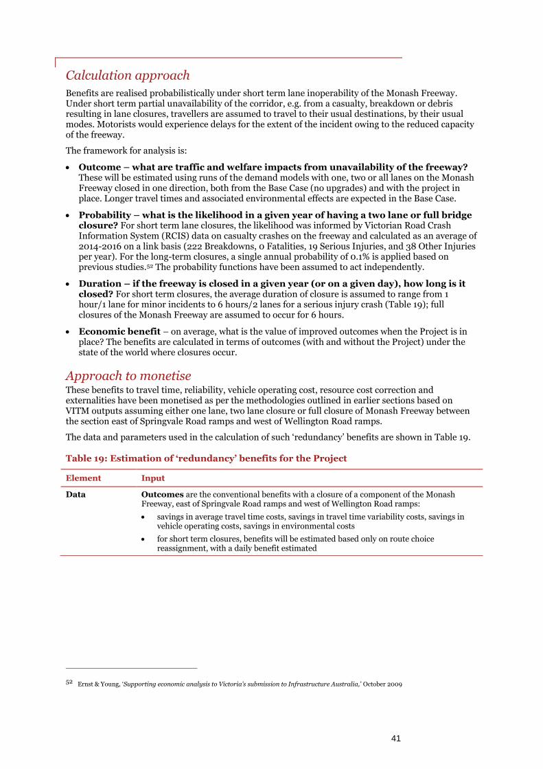
VicRoads PwC 41
Calculation approach
Benefits are realised probabilistically under short term lane inoperability of the Monash Freeway. Under short term partial unavailability of the corridor, e.g. from a casualty, breakdown or debris resulting in lane closures, travellers are assumed to travel to their usual destinations, by their usual modes. Motorists would experience delays for the extent of the incident owing to the reduced capacity of the freeway.
The framework for analysis is:
Outcome – what are traffic and welfare impacts from unavailability of the freeway? These will be estimated using runs of the demand models with one, two or all lanes on the Monash Freeway closed in one direction, both from the Base Case (no upgrades) and with the project in place. Longer travel times and associated environmental effects are expected in the Base Case.
Probability – what is the likelihood in a given year of having a two lane or full bridge closure? For short term lane closures, the likelihood was informed by Victorian Road Crash Information System (RCIS) data on casualty crashes on the freeway and calculated as an average of 2014-2016 on a link basis (222 Breakdowns, 0 Fatalities, 19 Serious Injuries, and 38 Other Injuries per year). For the long-term closures, a single annual probability of 0.1% is applied based on previous studies.52 The probability functions have been assumed to act independently.
Duration – if the freeway is closed in a given year (or on a given day), how long is it closed? For short term closures, the average duration of closure is assumed to range from 1 hour/1 lane for minor incidents to 6 hours/2 lanes for a serious injury crash (Table 19); full closures of the Monash Freeway are assumed to occur for 6 hours.
Economic benefit – on average, what is the value of improved outcomes when the Project is in place? The benefits are calculated in terms of outcomes (with and without the Project) under the state of the world where closures occur.
Approach to monetise These benefits to travel time, reliability, vehicle operating cost, resource cost correction and externalities have been monetised as per the methodologies outlined in earlier sections based on VITM outputs assuming either one lane, two lane closure or full closure of Monash Freeway between the section east of Springvale Road ramps and west of Wellington Road ramps.
The data and parameters used in the calculation of such ‘redundancy’ benefits are shown in Table 19.
Table 19: Estimation of ‘redundancy’ benefits for the Project
Element Input
Data Outcomes are the conventional benefits with a closure of a component of the Monash Freeway, east of Springvale Road ramps and west of Wellington Road ramps:
savings in average travel time costs, savings in travel time variability costs, savings in vehicle operating costs, savings in environmental costs
for short term closures, benefits will be estimated based only on route choice reassignment, with a daily benefit estimated
52 Ernst & Young, ‘Supporting economic analysis to Victoria’s submission to Infrastructure Australia,’ October 2009

VicRoads PwC 42
Element Input
Parameters Probability of closure:
Monash Freeway lane closure 3 percent probability of one lane closure per year and 2 percent probability of two lane closure – this is based on VicRoads Incident Rate, Monash Freeway 2014-2016; and VicRoads advice on average response and clearing times for freeway incidents. Short term closures are assumed to happen independent of one another.
Incident type Frequency
/year Avg. lane closure
Average duration
Fatality 0 Full closure 6 hours
Serious injury 19
2 lanes 6 hours
Other injury 38 2 lanes 2 hours
Break downs – cars, trucks and buses
222 1 lane 1 hour
Source: VicRoads Incident Rate, Incident on Freeway 2014- 2016; VicRoads advice on lane closure, average response and clearing times for freeway incidents.
Monash Freeway full closure probability of 0.2 percent per year (all lanes) assuming a half day closure every 5 years and a 0.1% probability closure.
Calculation The Road Link benefits in the ‘closure’ states of the world are combined with the core benefits (obtained in the state of the world where the Monash Freeway operates without closures) using an adjustment to the annualisation factor.
For example, for a Monash Freeway closure from breakdowns that occur for 1 hour 222 times a year, the closure states of the world occur, on average, for a total of 9 days of the year. As such, under just short term closures, with an annualisation factor of 320, the daily core benefits are multiplied by 311 (= 320 – 9), while the daily benefits of the Monash Freeway during a one lane closure apply for 9 days per year.
Source: PwC, 2017
6.6 Residual value of assets Residual values are recognised in the last year of the evaluation period to represent the unused portion of assets that have lives greater than the evaluation period.
Calculation approach The residual value is calculated using straight-line depreciation based on current Victorian Government guidance. The capital cost is broken into eight broad categories of assets namely: indirect cost, earthworks, pavements, concrete structures, steel structures and information technology. Indicative asset lives from ATC 2006 NGTSM53 were used to calculate asset value at the end of the appraisal period using straight line depreciation of assets.
Monetisation approach Cost were provided by VicRoads/Aquenta in six broad categories namely: indirect, earthworks, pavements, concrete structures, steel structures and information technology (including cabling and infrastructure). As show below the indicative asset lives from ATC 2006 NGTSM54 were used to
53 Australian Transport Council (ATC), National Guidelines for Transport System Management in Australia, 2006, vol. 4, Table 1.5.4:Typical
economic lives for infrastructure assets, p. 44
54 Australian Transport Council (ATC), National Guidelines for Transport System Management in Australia, 2006, vol. 4, Table 1.5.4:Typical
economic lives for infrastructure assets, p. 44
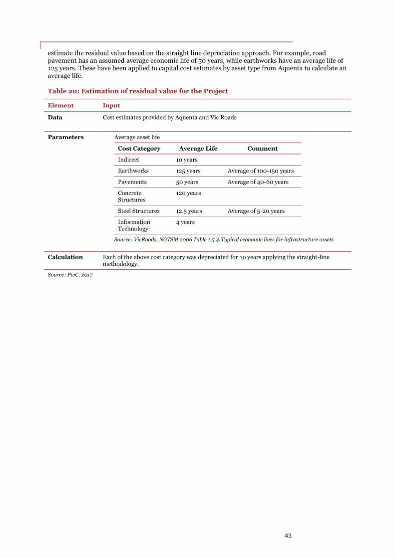
VicRoads PwC 43
estimate the residual value based on the straight line depreciation approach. For example, road pavement has an assumed average economic life of 50 years, while earthworks have an average life of 125 years. These have been applied to capital cost estimates by asset type from Aquenta to calculate an average life.
Table 20: Estimation of residual value for the Project
Element Input
Data Cost estimates provided by Aquenta and Vic Roads
Parameters Average asset life
Cost Category Average Life Comment
Indirect 10 years
Earthworks 125 years Average of 100-150 years
Pavements 50 years Average of 40-60 years
Concrete Structures
120 years
Steel Structures 12.5 years Average of 5-20 years
Information Technology
4 years
Source: VicRoads, NGTSM 2006 Table 1.5.4:Typical economic lives for infrastructure assets
Calculation Each of the above cost category was depreciated for 3o years applying the straight-line methodology.
Source: PwC, 2017

VicRoads PwC 44
6.7 Wider economic benefits Wider economic benefits (WEBs) are improvements in economic welfare that are not typically captured in the traditional cost benefit analysis. These benefits to productivity and labour markets arise from changes in accessibility resulting from transport interventions
The Monash Freeway Upgrade will boost productivity through improved travel times. The reduced travel time during peak hours as described in Section 6.2.1 and in particular to key employment clusters will encourage more people to join the workforce and seek employment. As an example, Figure 15 and Figure 16 indicate that as a result of the project there is a 4 to 5 percent decrease in travel time for trips originating from the key employment clusters – Monash and Melbourne CBD to Dandenong and Pakenham.
Figure 15: Impact on travel time Monash as origin 2031 Project Case compared to Base Case
Source: SGS analysis based on WSP modelling results using Victorian Integrated Transport Model (VITM), 2031 Option 3 compared to Base Case (2017)

VicRoads PwC 45
Figure 16:Impact on travel time CBD as origin 2031 Project Case compared to Base Case
Source: SGS analysis based on WSP modelling results using Victorian Integrated Transport Model (VITM), 2031 Option 3 compared to Base Case (2017)
The improvement during inter-peak hours will translate to an increase in business productivity. This productivity increase can also impact the distribution of employment opportunities, resulting in redistribution of some of Melbourne’s expected growth towards the outer south-east. The Project Case will create agglomeration benefits by improving the accessibility between businesses and higher labour supply productivity benefits.
The Australian Transport Assessment and Planning (ATAP) has recently released a framework for Wider Economic Benefits which is still a draft document for discussion.55 Noting that few concerns have been raised by practitioners in the method suggested by ATAP, PwC has based the methodology on United Kingdom Webtag guidance.
Three sets of WEBs have been considered in this report:
1) WEB1 – Agglomeration impacts (productivity benefits from firms being closer to markets)
2) WEB2 – Labour market impacts (reducing travel costs can have labour supply impacts and can move labour to more or less productive jobs)
3) WEB3 – Output change in imperfectly competitive markets (productivity benefits from firms facing increased competition)
6.7.1 Agglomeration
Agglomeration impacts refer to the affects achieved from the concentration of economies over an area. This is a major factor why cities exist as a centripetal force of urban development rather than the population spreading homogenously across the landscape. Firms derive productivity benefits from
55 Australian Transport Council (ATC), June 2017, Measuring WEBs in Australian Cities

VicRoads PwC 46
being close to one another and from being located in large labour markets. This proximity relates not merely to distance but to greater accessibility from reduced travel time.
In general, transport projects improve accessibility by reducing travel time and consequently bringing economies closer. The increased access to larger product, input and labour markets generates productivity benefits from increased opportunities for input sharing, knowledge/technology spillovers and output sharing.
Calculation approach The calculation approach to measure agglomeration impacts has been based on effective density and productivity changes using Webtag guidance. Effective density, which represents agglomeration, is a function of the generalised cost for business travel and commuting travel. Changes to effective density occur because of changes in generalised travel costs. Next, productivity changes were calculated as a response to the level of effective density between the scenarios. An elasticity of productivity with respect to effective density was applied for each industry sector
Approach to monetisation The data and parameters used in the calculation of agglomeration benefits are shown in Table 21. Intermediate calculations have been performed at the matrix level using VITM output (see Appendix B).
Table 21: Estimation of agglomeration benefits
Element Input to monetise
Data Employment (E) forecasts from VITM land use by:
Travel zone
Industry – using the Australian and New Zealand Standard Industrial Classification (ANZSIC)
GDP per worker (GDPW) using ATAP values with concurrence to VITM travel zones
estimated by SGS Economics & Planning56
Generalised travel costs (g), reflecting the costs of travel estimated in the demand model in the inter-peak only, by:
Travel zone – full matrices of origins and destinations
Mode – car and public transport (logsum)
Parameters Elasticity of productivity (𝝆𝒌), linking output and effective density of the employment location based on TfNSW guidelines for Australia ILTS (see Table 31).
Distance decay parameter (𝜶𝒌), has been set at 1
Calculation The simplified calculation for a single location (i) in a single forecast year (f), for a given industry (k) assuming the decay factor is 1:
𝑊𝐸𝐵1𝑖𝑓
= ∑
[
(
∑𝐸𝑗
𝑓
𝑔𝑖,𝑗𝐴,𝑓𝑗
∑𝐸𝑗
𝑓
𝑔𝑖,𝑗𝐵,𝑓𝑗
)
𝜌𝑘
− 1
]
𝑘
𝐺𝐷𝑃𝑊𝐵,𝑘,𝑓𝐸𝑖𝐵,𝑘,𝑓
Here, i is the travel zone under consideration and j is every other travel zone and modes are represented by m. Total agglomeration benefits are calculated by aggregating benefits across industries and zones (i). The benefits are calculated for each forecast year (see Appendix B for more details).
Source: PwC 2017 and Webtag Appraisal of Productivity Impacts Tag Unit A2.4
56 KPMG, 2015, Estimating WEBs of Transport Projects, 27 July 2015, page 48; Australian Transport Assessment and Planning (ATAP)
Guidelines, Measuring WEBs in Australian cities, June 2017, s3.2.3
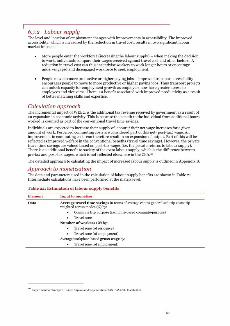
VicRoads PwC 47
6.7.2 Labour supply The level and location of employment changes with improvements in accessibility. The improved accessibility, which is measured by the reduction in travel cost, results in two significant labour market impacts:
More people enter the workforce (increasing the labour supply) – when making the decision to work, individuals compare their wages received against travel cost and other factors. A reduction in travel cost can thus incentivise workers to work longer hours or encourage under-engaged and disengaged workforce to seek employment.
People move to more productive or higher paying jobs – improved transport accessibility encourages people to move to more productive or higher paying jobs. Thus transport projects can unlock capacity for employment growth as employers now have greater access to employees and vice versa. There is a benefit associated with improved productivity as a result of better matching skills and expertise.
Calculation approach The incremental impact of WEB2, is the additional tax revenue received by government as a result of an expansion in economic activity. This is because the benefit to the individual from additional hours worked is counted as part of the conventional travel time savings.
Individuals are expected to increase their supply of labour if their net wage increases for a given amount of work. Perceived commuting costs are considered part of this net (post-tax) wage. An improvement in commuting costs can therefore result in an expansion of output. Part of this will be reflected as improved welfare in the conventional benefits (travel time savings). However, the private travel time savings are valued based on post-tax wages (i.e. the private returns to labour supply). There is an additional benefit to society of the extra labour supply, which is the difference between pre-tax and post-tax wages, which is not reflected elsewhere in the CBA.57
The detailed approach to calculating the impact of increased labour supply is outlined in Appendix B.
Approach to monetisation The data and parameters used in the calculation of labour supply benefits are shown in Table 21. Intermediate calculations have been performed at the matrix level.
Table 22: Estimation of labour supply benefits
Element Input to monetise
Data Average travel time savings in terms of average return generalised trip costs trip weighted across modes (G) by:
Commute trip purpose (i.e. home-based commute-purpose)
Travel zone
Number of workers (W) by:
Travel zone (of residence)
Travel zone (of employment)
Average workplace-based gross wage by:
Travel zone (of employment)
57 Department for Transport, ‘Wider Impacts and Regeneration, TAG Unit 2.8d,’ March 2011

VicRoads PwC 48
Element Input to monetise
Parameters Elasticity of labour supply with respect to effective wages (net of taxes and other transport costs) (εLS) of 0.1 has been found for the UK labour market.58
Lower productivity of workers on the margin of the labour force (η) of 0.69, which is based on available UK evidence that new workers entering the workforce are 31 percent less productive than the average of the current workforce.59
Average tax rate on earnings () of 0.30 to convert the gross earnings into net earnings. This reflects the corporate tax rate in Australia
Calculation The additional output produced by new entrants to the labour force is calculated as shown below. However, only the 30 percent tax wedge of this new output is genuinely additional to the welfare gain made by the employees that is already captured in private travel time savings and therefore the output is multiplied by 0.3060:
𝐺𝐷𝑃𝑓 = ∑∑[−𝜀𝐿𝑆 ((𝐺𝑖,𝑗
𝐴,𝑓− 𝐺𝑖,𝑗
𝐵,𝑓)Ω𝑗
𝑆,𝑓
(1 − 𝜏)𝑦𝑗𝑓
)𝑊𝑖,𝑗𝑆,𝑓
𝜂𝐺𝐷𝑃𝑊𝑗𝑆,𝑓
]
𝑗𝑖
where i is the travel zone of residence, j is the travel zone of employment, and G is the generalised daily return commuting costs from i to j.
Source: PwC, 2017
6.7.3 Imperfect competition Imperfections in product markets mean that firms can charge more for a good or service than it costs to produce. Labour costs in such markets underestimate labour productivity and, therefore, the value of business time savings. The ‘imperfect competition’ benefit of the options accounts for the gap between wages and labour productivity by scaling up the conventional ‘perfect competition’ estimate of business travel time savings.
Calculation approach An up-rate factor is applied to the value of business time savings (both average and variability). 61 This up-rate factor is a combination of the cost-price margin (how imperfect is the market) and the elasticity of demand in the imperfect market (by how much does output rise following a reduction in time savings).
Ideally, the up-rate factor is calculated for each sector or industry within the model; however, in reality this is not plausible. In the UK, the Department for Transport reviewed a number of estimated of price-cost margins within the UK economy. Based on the best estimates available they suggest an imperfect competition ‘up-rate’ parameter of one tenth, or 10%, be applied to the traditional value of business travel times.62 This is based on a price-cost margin of 0.2 and an elasticity of demand of 0.5.
In Australia, data suggests that the imperfect competition parameter may be higher due to a greater degree of market concentration. This concentration implies firms may be able to charge high mark-ups over their marginal costs (in this case the price of labour). However, the conservative UK estimate of 0.1 is applied.
58 UK Department for Transport, Tag Unit A2.4, September 2016, Appraisal of Employment Effects
59 Gregg, P., Johnson, P. and Reed H. ‘Entering work and the British tax and benefit system’, 1999
60 Adapted from Department for Transport, ‘The Wider Impact Sub-Objective, TAG Unit 3.5.14’, August 2012, p. 15 eq. 4.1a
61 Department for Transport, ‘The Wider Impact Sub-Objective, TAG Unit 3.5.14’, May 2012
62 Department for Transport, Transport, Wider Economic Benefits and Impacts on GDP, 2006, p 26.

VicRoads PwC 49
Approach to monetise The data and parameters used in the calculation of imperfect competition benefits are shown in Table 23. Direct benefits accruing to business purpose cars estimated elsewhere in the CBA are multiplied by a factor of 0.1 to quantify imperfect competition benefits.

VicRoads PwC 50
Table 23: Estimation of imperfect competition benefits
Element Input to monetise
Data Average travel time savings and vehicle operating cost savings (conventional benefit) and perceived travel time benefits by:
Business trip purpose (i.e. work-based work-purpose)
Parameters Up rate factor (τ) of 0.1, reflecting the degree to which demand will respond to a change in input costs:
EDP
MCP
, where
P
MCP is the representative price-cost margin (with price (P) and marginal cost (MC ))
assumed to be 0.2
ED is the representative elasticity of demand assumed to be 0.5
Calculation Additional output = τ (business user benefits)
The benefits are calculated for business benefits for each forecast year.
Source: PwC, 2017

VicRoads PwC 51
7 Economic Analysis Results
7.1 Summary of CBA results The economic appraisal of Bundle 3A and 3B are summarised below (Table 24). Economic analysis indicates that whilst both the preferred Bundle 3A and Bundle 3B deliver substantial benefits, Bundle 3A favourably yields higher benefits cost ratio than Bundle 3B. The benefits from the additional works around Oshea Road in Bundle 3A are expected to be significantly higher than the corresponding cost resulting in a higher BCR than Bundle 3B. The benefits for road users and freight are significant due to reduced travel times, lower vehicle operating costs, and improved reliability. The broader community will also benefit from improved transport network resilience and redundancy and improved liveability. In addition, the Project will generate wider economic benefits such as agglomeration benefits and improved accessibility to jobs.
To align with Victorian guidelines, the results for wider economic benefits (WEBs) and improvement in the perceived cost of congestion are presented separately outside the core economic appraisal results. Sensitivity tests were also undertaken to align with Infrastructure Australia’s assessment framework.
The key findings are:
The largest single benefit is travel time savings to existing users, indicating that existing car users rather than new users are main beneficiaries of the project.
The additional freeway lanes on the Monash Freeway from Warrigal Road to Eastlink (outbound) and Eastlink to Springvale Road (inbound) are expected to reduce congestion in the vicinity of the proposed works, in particular resulting in travel time savings for cars user commuting to Monash. Similarly for Bundle 3B the works around Oshea Road and Beaconsfield Interchange is expected to provide travel time benefits to people commuting to and from Dandenong and Cardinia.
The preferred Bundle 3A has higher capital investment than Bundle 3b to deliver the additional works to duplicate and extend Oshea Road from Clyde Road to Beaconsfield Interchange. However Bundle 3A which provides improved access to the south-east growth area, has a higher net present value and benefit cost ratio, indicating that the additional investment delivers even better outcomes for the community compared to Bundle 3B.

VicRoads PwC 52
Table 24: Cost benefit analysis results for the Project ($ June 2017 millions, real, discounted present values)
Costs and benefits Bundle 3A Bundle 3B
Costs Capital costs 498 95% 415 92%
Operating and maintenance costs 25 5% 21 8%
Sub-total costs 523 100% 436 100%
Benefits Transport user benefits
Travel time savings 1,381 58% 1,029 61%
Vehicle operating cost savings 680 28% 460 27%
Improved reliability 255 11% 180 11%
Resilience to lane closures 93 4% 70 4%
Safety and environment benefits
Crash Cost Savings (incl impact of managed motorways)
36 2% 27 2%
Environmental benefits -68 -3% -80 -5%
Residual value 17 1% 14 1%
Sub-total Benefits 2,394 100% 1,700 100%
Results Benefit Cost Ratio 4.6 3.9
Net Present Value 1,871 1,264
Additional Benefits (non-core benefits)
Additional Benefits related to Productivity and Growth for Melbourne
Travel time benefits from improved perceived congestion
19 1% 32 2%
Economic development in Melbourne
Agglomeration 211 7% 150 7%
Labour supply 9 <1% 6 <1%
Imperfect competition 217 8% 157 7%
Results including WEBs
Total Benefits including WEBs and improved perceived congestion benefit
2,853 2,045
Benefit Cost Ratio including WEBs and improved perceived congestion benefit
5.5 4.7
Net Present Value including WEBs 2,330 1,609
*Note: the costs represent final risk adjusted cost and differ from out-turn capital cost estimates as they have been adjusted for inclusion in the economic appraisal to represent real, discounted (present value) costs over the lifecycle. Bundle 3B resilience, crash cost and WEBs benefits estimated based on Bundle 3 model runs. Note: estimated incremental to the Base Case, discounted based on a 7% real discount rate, based on P50 final risk adjusted capital and operating costs, benefit appraisal period 2022/23 to 2052/53. Source: PwC, 2017
7.2 Sensitivity analysis of CBA results This section outlines the results of a number of sensitivity test undertaken to test the robustness of the economic viability of the Project in response to changes in key assumptions.

VicRoads PwC 53
7.2.1 Sensitivities for Infrastructure Australia
As described in Section 2, the methodology for the economic assessment has been developed reflecting both Victorian guidelines and Infrastructure Australia guidelines. However there were two instances where alignment with both guidelines was no possible. This has been addressed by the below two sensitivity tests.
Do-minimum Base Case
The Transport Network Base Case represents the Victorian Government Reference Case which is a combination of committed and planned projects. The network is considered by the state to represent the most realistic transport infrastructure development to support the population, employment, and transport outcomes expected to occur in Victoria (Table 35).
A sensitivity test based on Infrastructure Australia (IA) requirements was undertaken using a do-minimum Base Case which excludes un-committed projects. In 2031, some of the key projects excluded from the network were Dandenong Bypass, South Gippsland Freeway ramp to Hallam Bypass, Westall Road extension, North East Link, Tullamarine Freeway extension, Bulla Road bypass, Hume Freeway upgrades and Eastern Freeway upgrades. The 2051 network excluded Eastlink upgrades, Outer Metropolitan Ring Road, Western Freeway Upgrades.
The results in the do-minimum scenario show higher benefits than the core run (refer Table 25), mainly due to benefits from unassigned public transport (PT) trips. The 2051 do-minimum scenario assumes the 2031 do-minimum PT services (i.e. no PT service improvements between 2031 and 2051) and results in the daily excess PT demand increasing dramatically from 5,000 (2051 base case) to 28,000 (2051 do-minimum). In the VITM excess PT trips are those which are unable to readily reach their destination due to capacity constraint on PT network as part of crowd modelling. Thus, the PT system is unable to satisfy the excess demand which then flows onto the road network.
Table 25: Economic appraisal of the preferred Bundle (June 2017 $millions, real, discounted present values) – Do-minimum Base Case
Costs and Benefits Project Scope, Bundle 3A
Core Results
PV ($m)
Do-minimum
Base Case
PV ($)
Total Cost 523 523
Benefits 2,394 3,327
Net Present Value 1,871 2,804
Benefit Cost Ratio 4.6 6.4
Note: the costs differ from out-turn capital cost estimates as they have been adjusted for inclusion in the economic appraisal to represent real, discounted (present value) costs over the lifecycle Note: estimated incremental to the Base Case, discounted based on a 7% real discount rate, based on P50 capital and operating costs, excludes WEBS and Improved Perceived Congestion Benefit, Resilience Benefits estimated from Core Results. Do-minimum Base Case benefits for resilience and crash cost and WEBs benefits estimated based on Bundle 3 core model runs. Source: PwC, 2017
Vehicle Operating Cost
A sensitivity was undertaken to satisfy Infrastructure Australia by calculating vehicle operating cost savings based on Austroads 2012 guidelines. This differs from the core results which base the calculations on Australian Transport Assessment and Planning 2016 guidelines as per Victorian Government recommendations.
The results from the analysis (see Table 26) demonstrate lower vehicle operating saving benefits when applying the Austroads guidelines.

VicRoads PwC 54
Table 26: Economic appraisal of the preferred Bundle (June 2017 $millions, real, discounted present values) – Austroad 2012 VOC
Costs and Benefits Project Scope, Bundle 3A
Core Results
PV ($m)
IA sensitivity
PV ($)
Total Cost 523 523
Benefits 2,394 2,286
Net Present Value 1,871 1,763
Benefit Cost Ratio 4.6 4.4
Note: Vehicle operating cost calculated at an aggregate level and not on a link by link basis. The costs differ from out-turn capital cost estimates as they have been adjusted for inclusion in the economic appraisal to represent real, discounted (present value) costs over the lifecycle. Note: estimated incremental to the Base Case, discounted based on a 7% real discount rate, based on P50 final risk adjusted capital and operating costs, benefit appraisal period FY23 to FY52, excludes WEBS and Improved Perceived Congestion Benefit Source: PwC, 2017
7.2.2 Other Sensitivities
Sensitivities were also performed on key economic appraisal inputs and assumptions as shown in Table 27
Table 27: Sensitivity testing of economic appraisal results on Bundle 3A
Sensitivity Test for Bundle 3A BCR
Core Results (from Table 24) 4.6
Discount Rate
4% discount rate 6.9
10% discount rate 3.2
Project Cost
P90 Costs 4.4
+20% P50 Costs 3.8
-20% P50 Costs 5.7
Annualisation
+10% 5.0
-10% 4.1
Benefits
+20% benefits 5.6
-20% benefits 3.7
Productivity Growth
Exclude real growth 4.0
Construction Disruption
Construction distruption impact 4.1
Best Case Scenario
P50 cost, do-minimum base case, +10% annualisation, ATAP VOC
approach
7.0
Worst Case Scenario

VicRoads PwC 55
Sensitivity Test for Bundle 3A BCR
P90 cost, do-minimum base case, -10% annualisation, Austroad VOC
approach
3.3
*Note: the costs differ from out-turn capital cost estimates as they have been adjusted for inclusion in the economic appraisal to represent real, discounted (present value) costs over the lifecycle. Note: estimated incremental to the Base Case, discounted based on a 7% real discount rate, based on P50 final risk adjusted capital and operating costs, benefit appraisal period FY23 to FY52, excludes WEBS and Improved Perceived Congestion Benefit Source: PwC, 2017

VicRoads PwC 56
Appendices
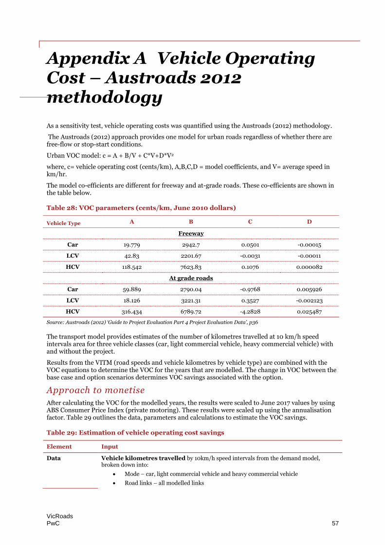
VicRoads PwC 57
Appendix A Vehicle Operating Cost – Austroads 2012 methodology
As a sensitivity test, vehicle operating costs was quantified using the Austroads (2012) methodology.
The Austroads (2012) approach provides one model for urban roads regardless of whether there are free-flow or stop-start conditions.
Urban VOC model: c = A + B/V + C*V+D*V2
where, c= vehicle operating cost (cents/km), A,B,C,D = model coefficients, and V= average speed in km/hr.
The model co-efficients are different for freeway and at-grade roads. These co-efficients are shown in the table below.
Table 28: VOC parameters (cents/km, June 2010 dollars)
Vehicle Type A B C D
Freeway
Car 19.779 2942.7 0.0501 -0.00015
LCV 42.83 2201.67 -0.0031 -0.00011
HCV 118.542 7623.83 0.1076 0.000082
At grade roads
Car 59.889 2790.04 -0.9768 0.005926
LCV 18.126 3221.31 0.3527 -0.002123
HCV 316.434 6789.72 -4.2828 0.025487
Source: Austroads (2012) ‘Guide to Project Evaluation Part 4 Project Evaluation Data’, p36
The transport model provides estimates of the number of kilometres travelled at 10 km/h speed intervals area for three vehicle classes (car, light commercial vehicle, heavy commercial vehicle) with and without the project.
Results from the VITM (road speeds and vehicle kilometres by vehicle type) are combined with the VOC equations to determine the VOC for the years that are modelled. The change in VOC between the base case and option scenarios determines VOC savings associated with the option.
Approach to monetise
After calculating the VOC for the modelled years, the results were scaled to June 2017 values by using ABS Consumer Price Index (private motoring). These results were scaled up using the annualisation factor. Table 29 outlines the data, parameters and calculations to estimate the VOC savings.
Table 29: Estimation of vehicle operating cost savings
Element Input
Data Vehicle kilometres travelled by 10km/h speed intervals from the demand model, broken down into:
Mode – car, light commercial vehicle and heavy commercial vehicle
Road links – all modelled links

VicRoads PwC 58
Element Input
Parameters Vehicle operating cost equations:
c = A + B/V + C*V+D*V2
where, c= vehicle operating cost (cents/km), A,B ,C,D = model coefficients, and V= average speed in km/hr.
Calculation 𝑉𝑒ℎ𝑖𝑐𝑙𝑒 𝑜𝑝𝑒𝑟𝑎𝑡𝑖𝑛𝑔 𝑏𝑒𝑛𝑒𝑓𝑖𝑡 = 𝑁𝑒𝑡𝑤𝑜𝑟𝑘 𝑉𝑂𝐶𝑤𝑖𝑡ℎ𝑜𝑢𝑡 𝑝𝑟𝑜𝑗𝑒𝑐𝑡 − 𝑁𝑒𝑡𝑤𝑜𝑟𝑘 𝑉𝑂𝐶𝑜𝑝𝑡𝑖𝑜𝑛
Estimated VOC values were inflated to June 2017 dollars using ABS Melbourne Consumer Price Index (private motoring). The benefits were calculated for each of the modelled time periods and then scaled to annual values using the annualisation factor to reach an annual value for the forecast year.
Source: PwC, 2017 based on Austroads (2012) ‘Guide to Project Evaluation Part 4 Project Evaluation Data’ p36

VicRoads PwC 59
Appendix B Wider Economic Benefits
Agglomeration impact calculation The additional output attributable to an improvement in transport accessibility of linked employment areas relies on the concept of ‘effective job density’. The effective job density, EJD, of a given employment area, i, is the sum of all of the employment within all other areas, but where this employment is weighted according to how easily its location is reached from i. That is, the effective density of area i in industry k is estimated as:
𝐸𝐽𝐷𝑖𝑘 = ∑
𝐸𝑗𝑘
𝑔𝑗𝑚
𝑗,𝑚
where Ejk is the employment in an area linked to i, and gj
m is the generalised travel cost between i and j by mode m.
The calculation of the additional output from an improvement in effective density due to a transport project is not straightforward due to the different industry responses to increased effective density, the number of transport modes and the spatial diversity of employment location and accessibility changes. The agglomeration impacts were calculated by primarily following Webtag approach.63
Step 1: Estimate inter-peak logsum travel times in the base and project cases. The logsum approach is used to more accurately capture consumer surplus.64 The travel time was monetised using $16.52 as the value of time (see Table 11)65
𝑔𝑖,𝑗𝑆,𝑚,𝑝,𝑓
=𝑙𝑛 ∑ 𝑒(𝜆∙𝐺𝐶𝑖𝑗,𝑚)
𝑚
𝜆
Where: 𝜆 = scaling parameter (-0.3) 𝑚 = a transport mode 𝐺𝐶𝑖𝑗,𝑚 = interpeak travel time (mins) between origin i and destination j for mode m
𝐺𝐶𝑖𝑗,𝑃𝑇 = (𝐼𝑉𝑇𝑖𝑗 + 𝐴𝐸𝑇𝑖𝑗 ∙ 𝐹𝑎𝑐𝑡𝑜𝑟𝐴𝐸𝑇 + 𝑊𝐴𝑇𝑖𝑗 ∙ 𝐹𝑎𝑐𝑡𝑜𝑟𝑊𝐴𝑇)
𝐺𝐶𝑖𝑗,𝑐𝑎𝑟 = 𝑇𝑖𝑗
Where:
𝐼𝑉𝑇𝑖𝑗 = in vehicle time for public transport users from origin i to destination j
𝐴𝐸𝑇𝑖𝑗 = access and egress time for public transport users from origin i to destination j
𝐹𝑎𝑐𝑡𝑜𝑟𝐴𝐸𝑇 = additional factor for public transport users in access and egress time(1.4)66 𝑊𝐴𝑇𝑖𝑗 = wait time for public transport users from origin i to destination j
𝐹𝑎𝑐𝑡𝑜𝑟𝑊𝐴𝑇 = additional factor for public transport users wait time(1.4)67
63 UK Department for Transport, Tag Unit A2.4, September 2016, Appraisal of Productivity Impacts
64 Australian Transport Assessment and Planning (ATAP) Guidelines, Measuring WEBs in Australian cities, June 2017, s3.1.3
65 Non Business travel time was used as proxy for PT travel time as most of the travel time beneficiaries were car users.
66 Australian Transport Council ,2006 National Guidelines for Transport System Management in Australia,Table1.6.1 User Perceived cost unit
values

VicRoads PwC 60
𝑇𝑖𝑗= in vehicle time for car users from origin i to destination j
Step 2: Calculate effective density for each industry and each origin
𝑑𝑖𝑆,𝑘,𝑓
= ∑ ∑𝐸𝑗
𝑆,𝑓
(𝑔𝑖,𝑗𝑆,𝑚,𝑓
)^𝑎𝑘𝑚𝑗
Where
𝑑𝑖𝑠,𝑘,𝑓
= effective density for each industry and each origin
𝐸𝑗𝑠,𝑓
= total employment at each origin location travel zone
𝑔𝑖,𝑗𝑠,𝑚,𝑓
= generalised cost for each origin-destination pair
𝑎𝑘 = decay parameter by industry
Step 3: Calculate productivity impact for each industry and each origin
𝑊𝐸𝐵1𝑖𝑓
= ∑[(𝑑𝑖
𝐴,𝑘,𝑓
𝑑𝑖𝐵,𝑘,𝑓
)
𝜌𝑘
− 1]
𝑘
𝐺𝐷𝑃𝑊𝐵,𝑘,𝑓𝐸𝑖𝐵,𝑘,𝑓
Where
𝐺𝐷𝑃𝑊𝑖𝐵,𝑘,𝑓
= GDP per worker
𝐸𝑖𝐵,𝑘,𝑓
= Employment by sector
𝜌𝑘 = Productivity elasticity
Table 30: Agglomeration data sources
Item Source Notes
Decay parameter by industry Assumed as 1
Productivity elasticity TfNSW 2016 Guidelines68 Elasticity of productivity: Australia(ITLS)
Employment count VITM Land Use Modelling
GDP per worker ATAP values69 Concurrence to VITM travel zones completed by SGS Economics & Planning70
Trips Demand skims from VITM Inter-peak skims for car and public transport users
Source: PwC, 2017 calculations based on TfNSW (2016), ATAP (2017) and SGS Economics & Planning (2017)
67 Australian Transport Council ,2006 National Guidelines for Transport System Management in Australia,Table1.6.1 User Perceived cost unit
values
68 Transport for NSW, Principles and Guidelines for Economic Appraisals, 2016.
69Australian Transport Assessment and Planning (ATAP) Guidelines, Measuring WEBs in Australian cities, June 2017, s3.2.3
70 SGS Economics & Planning, Memo to PwC: ‘Average gross value added per work’, 9 September 2017

VicRoads PwC 61
Table 31: Elasticity of productivity parameters
Industry
ANZSIC 2006
categories
Elasticity of productivity:
Australia(ITLS)
Agriculture A 0.047
Mining B 0.163
Manufacturing C 0.035
Electricity, gas & water D 0.108
Construction E 0.051
Wholesale F 0.034
Retail G 0.003
Accommodation and Food Services H -0.011
Transport & storage I 0.044
Communications J 0.051
Finance and Insurance Services K 0.058
Rental Hiring and Real Estate Services L 0.057
Government Administration and Defence M 0.049
Education and Training N 0.047
Health Care and Community Service O 0.029
Cultural and Recreation Services R 0.032
Personal and Other Services S 0.007
Source: TfNSW (2016) Principles and Guidelines for Economic Appraisal of Transport Investment and Initiatives, page 72
Labour supply The tax revenue increase was calculated for increased labour supply using the following two step approach.71 Data sources for the calculation are set out in Table 32.
Step 1: Estimate the average round trip generalised cost of commuting (𝑮𝒊.𝒋)
Calculate the peak logsum travel times using the same equations as in Step 1 of agglomeration calculation replacing inter-peak with peak travel time skims.
Step 2: Estimate labour supply impact on GDP
𝐺𝐷𝑃𝑓 = ∑∑[−𝜀𝐿𝑆 ((𝐺𝑖.𝑗
𝐴,𝑓− 𝐺𝑖,𝑗
𝐵,𝑓)Ω𝑗
𝑆,𝑓
(1 − 𝜏1)𝑦𝑗𝑓
)𝑊𝑖,𝑗𝑆,𝑓
𝜂𝐺𝐷𝑃𝑊𝑗𝑆,𝑓
]
𝑗𝑖
Where G = average round trip generalised cost of
𝑦𝑗𝑓
= average annual gross income
𝑊𝑖,𝑗𝑆,𝑓
= workers living in origin and employed in j
𝜀𝐿𝑆 = elasticity of labour supply
Ω𝑗𝑆,𝑓
= average annual round trip commuting journeys
𝜏 = tax rate 𝜂 = lower productivity factor
𝐺𝐷𝑃𝑊𝑗𝑆,𝑓
= GDP per worker
71 UK Department for Transport, Web Tag Unit A2.4, September 2016, Appraisal of Employment Effects

VicRoads PwC 62
Step 3 Calculate Wider Impacts – Tax Wedge
𝑊𝑓 = 𝜏 ∗ 𝐺𝐷𝑃𝑓
Where 𝜏 = tax wedge of 30 percent based on Australian effective tax rate
Table 32: Labour supply data sources
Item Source Notes
Average gross weekly wage ABS average earnings72 Concurrence applied from SA2 to travel zone based on area size
Average annual round trip commuting journeys
240 Assuming only weekday work and four weeks annual leave
Workers at residence VITM demand modelling outputs
AM peak demand of blue collar and white collar
Working age population VITM Land use modelling
Elasticity of labour supply 0.1 - Webtag Equation 2 Labour Supply/Employment Impact
Lower productivity factor 0.69 - Webtag Equation 3 Labour Supply/Employment Impact
Tax take 30% - corporate tax rate in Australia73
Source: PwC, 2017 calculations based on ABS (2017), VITM (2017) and UK Department for Transport, Web Tag Unit A2.4, September 2016, Appraisal of Employment Effects
72 Australian Burearu of Statistics, ‘6302 – Average Weekly Earnings’, May 2017
73 Australian Taxation Office, Company tax rates 2016-17, 2017, accessible here: <https://www.ato.gov.au/Rates/Company-tax/>

© 2015 PricewaterhouseCoopers. All rights reserved. PwC refers to the Australian member firm, and may sometimes refer to the PwC network. Each member firm is a separate legal entity. Please see www.pwc.com/structure for further details. Liability limited by a scheme approved under Professional Standards Legislation
www.pwc.com.au