Molles: Ecology 2nd Ed.

POPULATION DISTRIBUTION AND ABUNDANCE

Chapter 9

Molles: Ecology 2nd Ed.

Chapter Concepts

• Physical environment limits geographic distribution of species

• On small scales, individuals within pops. are distributed in random, regular, or clumped patterns; on larger scales, individuals within pop. are clumped

• Population density declines with increasing organism size

• Rarity influenced by geographic range, habitat tolerance, pop. size; rare species vulnerable to extinction

Molles: Ecology 2nd Ed.

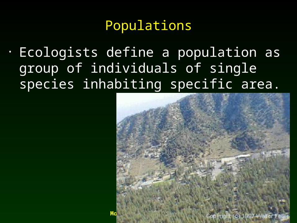
Populations

• Ecologists define a population as group of individuals of single species inhabiting specific area.

Molles: Ecology 2nd Ed.

Habitat

• Physical environmental conditions that allow individuals of species to survive AND reproduce

Molles: Ecology 2nd Ed.

Habitat quality

• Ability of environmental conditions to support repro and survival Habitat area/volume Resource concentration Time

• High habitat quality = organisms acquire many resources; high survival + repro = large pop.

Molles: Ecology 2nd Ed.

Population numbers vary with habitat quality

Po

pula

tion

siz

e

Environmental gradient

Low Optimal High

GoodhabitatPoor

habitatPoorhabitat

Molles: Ecology 2nd Ed.

Distribution Limits

• Physical environment limits geographic distribution of species Organisms can only compensate so much

for environmental variation

Molles: Ecology 2nd Ed.

Geographical range

• Geographic area where species is found Geographic area where species is found (based on macroclimate, salinity, nutrients, (based on macroclimate, salinity, nutrients, oxygen, light, etc.)oxygen, light, etc.)

Molles: Ecology 2nd Ed.

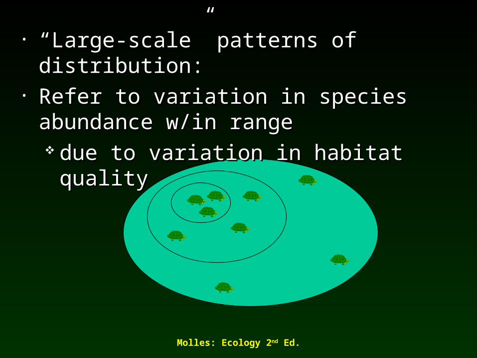
• ““Large-scale” patterns of distribution:Large-scale” patterns of distribution:• Refer to variation in species abundance w/in Refer to variation in species abundance w/in

rangerange due to variation in habitat qualitydue to variation in habitat quality

Molles: Ecology 2nd Ed.

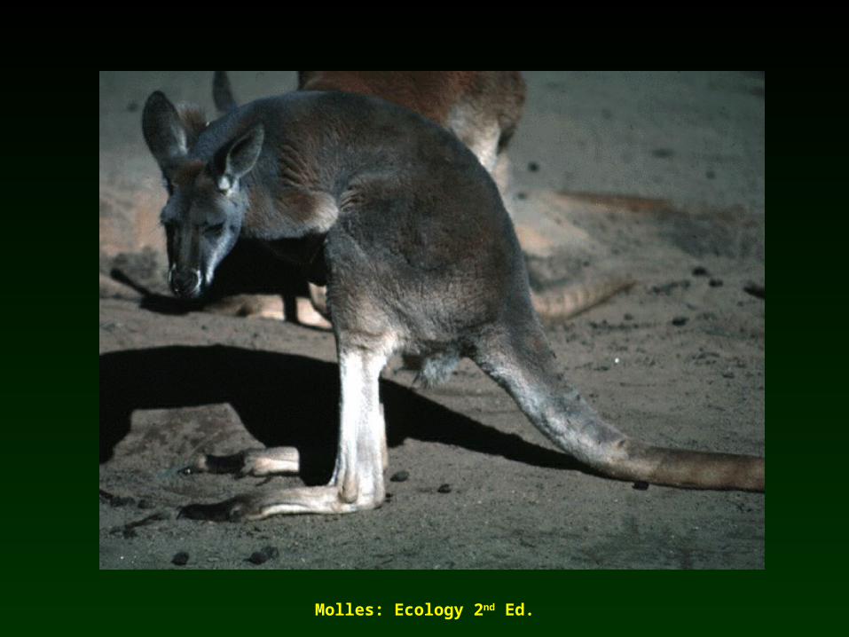
Kangaroo Distributions and Climate

• Caughley - relationship between climate + distribution of three largest kangaroos in Australia

Molles: Ecology 2nd Ed.

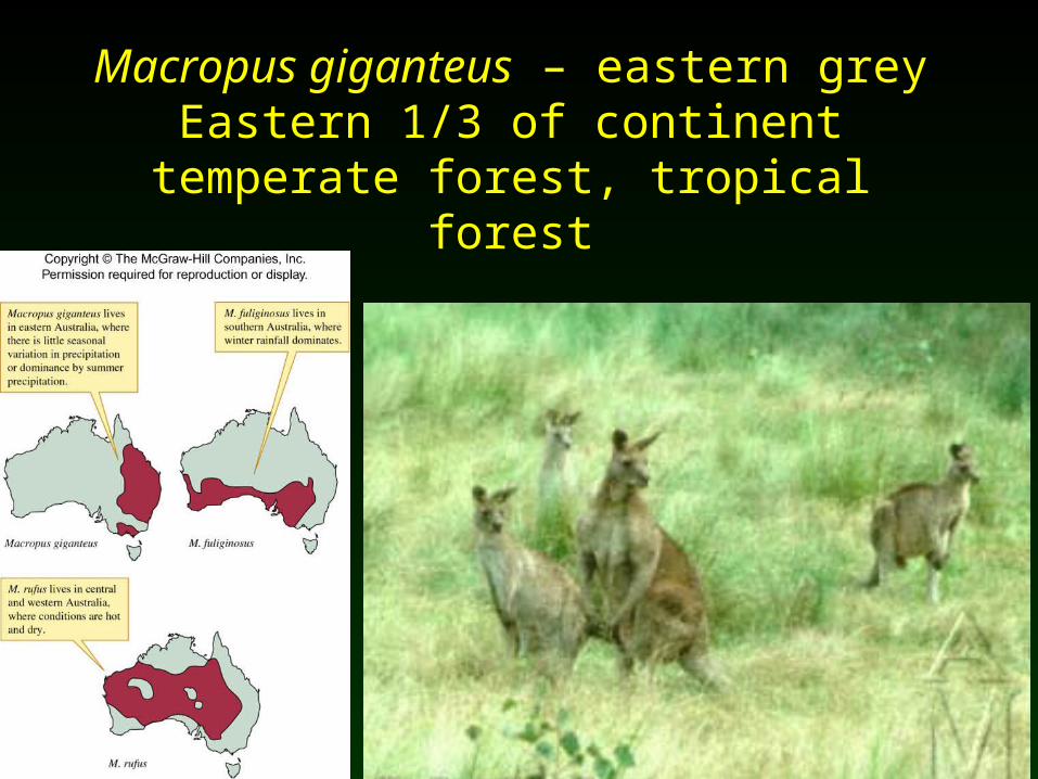
Macropus giganteus – eastern greyEastern 1/3 of continent

temperate forest, tropical forest

Molles: Ecology 2nd Ed.

Macropus fuliginosus – western grey southern and western regions

temperate woodlands and shrubs

Molles: Ecology 2nd Ed.

Macropus rufus – redarid / semiarid interior

Molles: Ecology 2nd Ed.

Fig 9.2Distributions largely based

on climate

Molles: Ecology 2nd Ed.

Kangaroo Distributions and Climate

• Limited distributions may not be directly determined by climate. Climate often influences species

distributions via: food production water supply habitat incidence of parasites, pathogens and

competitors

Molles: Ecology 2nd Ed.

Tiger Beetle of Cold Climates

• Tiger beetle (Tiger beetle (Cicindela longilabrisCicindela longilabris) - higher ) - higher latitudes + elevations than other NA specieslatitudes + elevations than other NA species SchultzSchultz found metabolic rates of found metabolic rates of C. C.

longilabrislongilabris are higher and preferred temps. are higher and preferred temps. lower than other specieslower than other species Physical env. limits species distributionsPhysical env. limits species distributions

Molles: Ecology 2nd Ed.

Fig 9.3

Metabolic rates of Metabolic rates of C. C. longilabrislongilabris higher; higher; preferred temps preferred temps lower than other lower than other beetle speciesbeetle species

Adapted to cool Adapted to cool climatesclimates

Molles: Ecology 2nd Ed.

Distributions of Plants Along a Moisture-Temperature Gradient

• Encelia spp. distributions + variations in temp and precipitation

Fig 9.7

Molles: Ecology 2nd Ed.

Fig 9.5

Molles: Ecology 2nd Ed.

Distributions of Barnacles - Intertidal Gradient

• Organisms in intertidal zone have evolved Organisms in intertidal zone have evolved different degrees of resistance to dryingdifferent degrees of resistance to drying Barnacles - distinctive patterns of zonation Barnacles - distinctive patterns of zonation

within intertidal zonewithin intertidal zone

Molles: Ecology 2nd Ed.

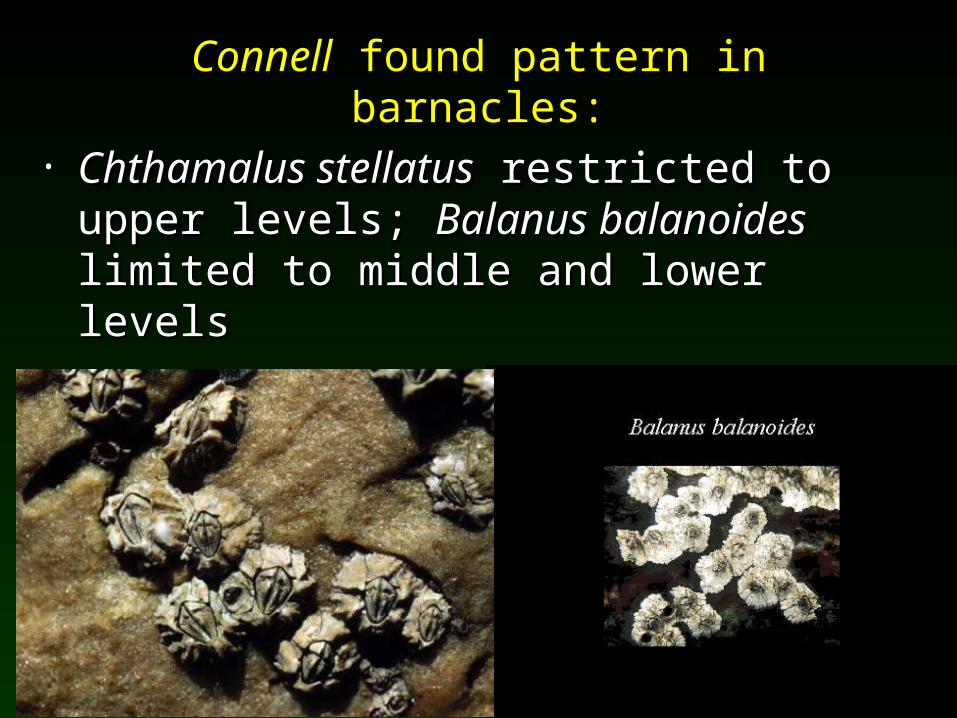
ConnellConnell found pattern in barnacles: found pattern in barnacles:

• Chthamalus stellatusChthamalus stellatus restricted to upper restricted to upper levels; levels; Balanus balanoidesBalanus balanoides limited to middle limited to middle and lower levelsand lower levels

Molles: Ecology 2nd Ed.

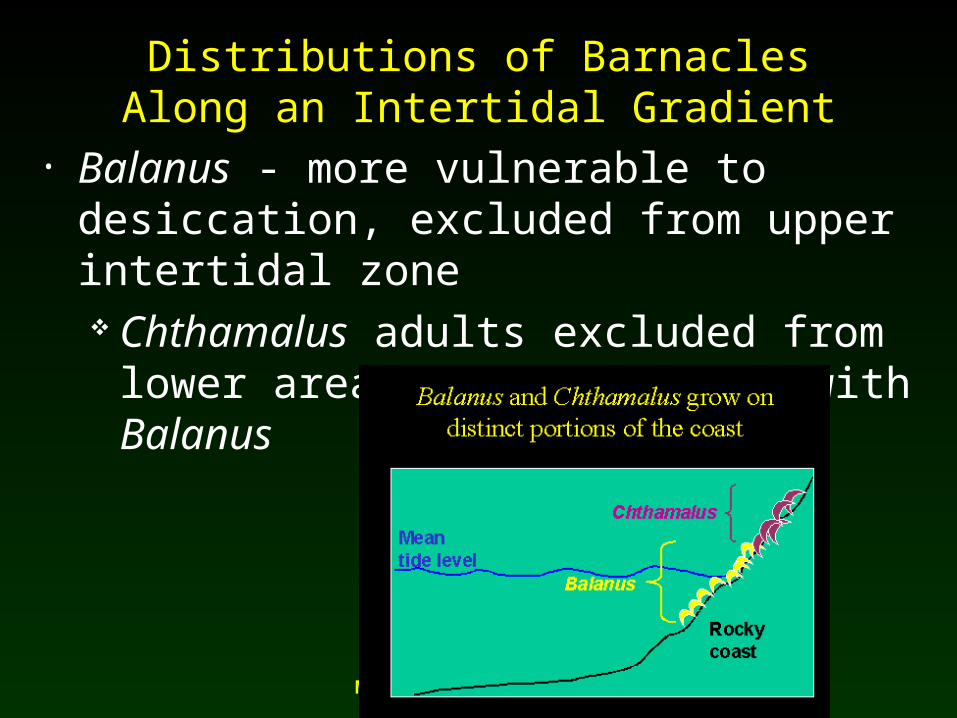
Distributions of Barnacles Along an Intertidal Gradient

• Balanus - more vulnerable to desiccation, excluded from upper intertidal zone Chthamalus adults excluded from lower

areas by competition with Balanus

Molles: Ecology 2nd Ed.

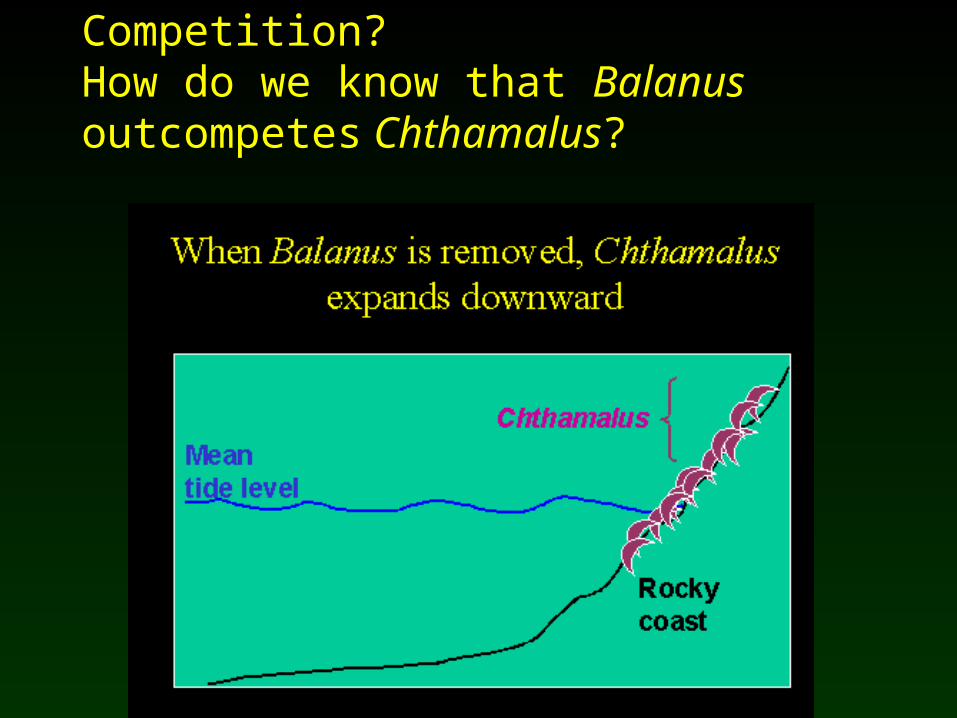
Competition? How do we know that Balanus outcompetes Chthamalus?

Molles: Ecology 2nd Ed.

Fig 9.8

Fig 9.9

Molles: Ecology 2nd Ed.

Distribution of Individuals on Small Scales• Three basic patterns:

Random: equal chance of being anywhere Regular: uniformly spaced

Exclusive use of areas Individuals avoid one another

Clumped: unequal chance of being anywhere Mutual attraction between individuals Patchy resource distribution

Molles: Ecology 2nd Ed.

Fig 9.10

Molles: Ecology 2nd Ed.

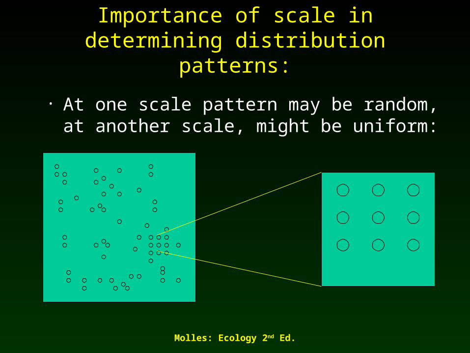
Importance of scale in determining distribution patterns:

• At one scale pattern may be random, at another scale, might be uniform:

Molles: Ecology 2nd Ed.

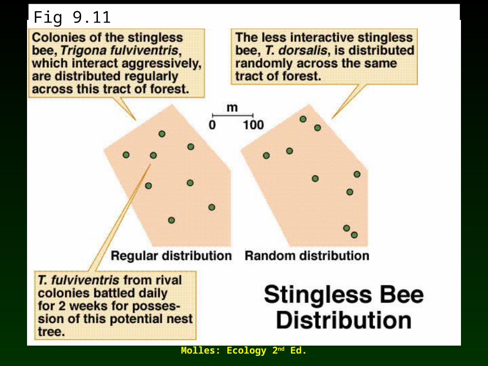
Distribution of Tropical Bee Colonies

• Hubbell and Johnson predicted aggressive bee colonies have regular distributions;

• Predicted non-aggressive species have random or clumped distributions

Molles: Ecology 2nd Ed.

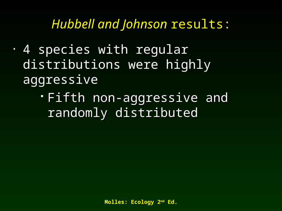
Hubbell and Johnson results:

• 4 species with regular distributions were highly aggressive

Fifth non-aggressive and randomly Fifth non-aggressive and randomly distributeddistributed

Molles: Ecology 2nd Ed.

Fig 9.11

Molles: Ecology 2nd Ed.

What causes overall pattern?

• Behavior!• Aggressive bees were uniformly spaced due

largely to their interactions.• Non-aggressive species were random - did

not interact.

Molles: Ecology 2nd Ed.

Fig 9.10

Molles: Ecology 2nd Ed.

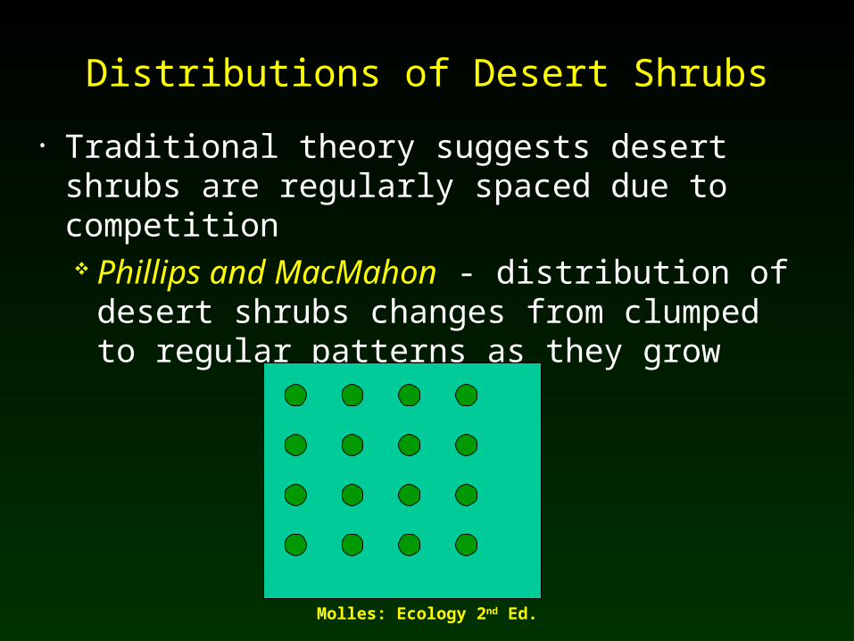
Distributions of Desert Shrubs

• Traditional theory suggests desert shrubs are regularly spaced due to competition Phillips and MacMahon - distribution of

desert shrubs changes from clumped to regular patterns as they grow

Molles: Ecology 2nd Ed.

Hypothesis:

Young shrubs clumped for (3) reasons: Seeds germinate at safe sites Seeds not dispersed from parent areas Asexual reproduction

Molles: Ecology 2nd Ed.

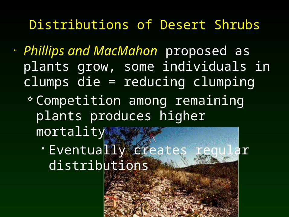
Distributions of Desert Shrubs

• Phillips and MacMahon proposed as plants grow, some individuals in clumps die = reducing clumping Competition among remaining plants

produces higher mortality Eventually creates regular distributions

Molles: Ecology 2nd Ed.

Fig 9.13 - their hypothesis

Molles: Ecology 2nd Ed.

Brisson and Reynolds

• Dug up roots, map distribution of 32 bushes• found competitive interactions with

neighboring shrubs influences distribution of creosote roots

Molles: Ecology 2nd Ed.

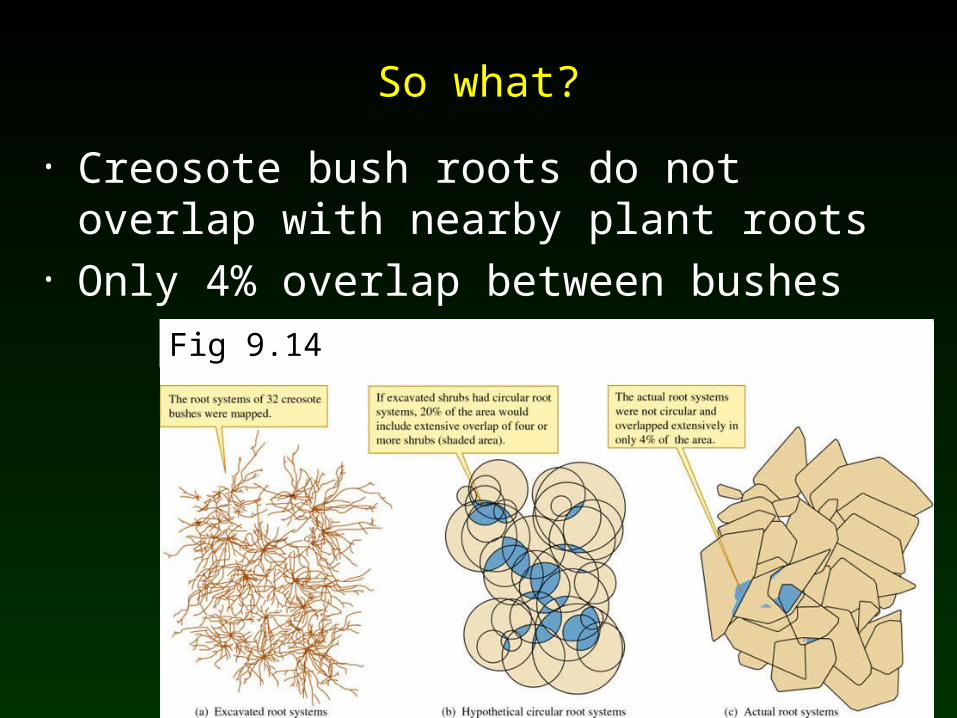
• Creosote bush roots do not overlap with nearby plant roots

• Only 4% overlap between bushes

Fig 9.14

So what?

Molles: Ecology 2nd Ed.

Distributions of Individuals on Large Scales

• Bird Pops North America Root - at continental scale, bird pops have

clumped distributions (Christmas Bird Counts)

Clumped patterns in species with widespread distributions

Fig 9.14

Molles: Ecology 2nd Ed.

Similar distribution pattern for species with small range: few “hot spots”

Fish crow

Fig 9.14

Molles: Ecology 2nd Ed.

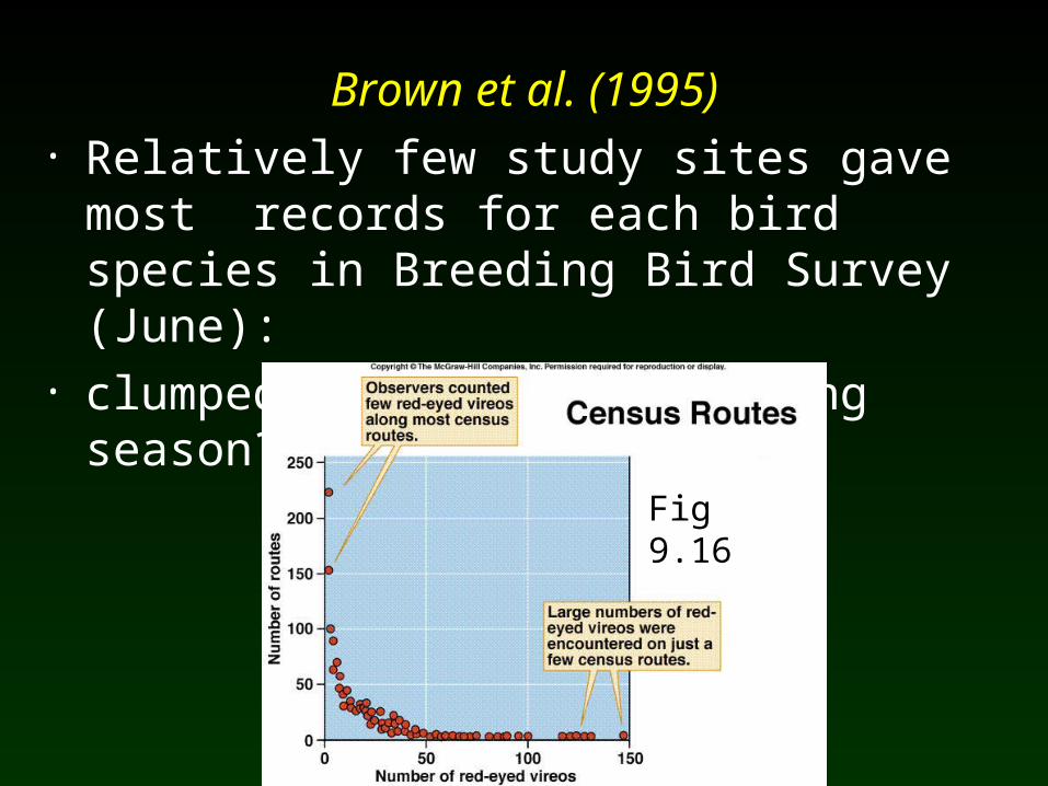
Brown et al. (1995)• Relatively few study sites gave most

records for each bird species in Breeding Bird Survey (June):

• clumped only during breeding season?

Fig 9.16

Molles: Ecology 2nd Ed.

Density = number individuals per unit area/volume

• Sedentary organisms: plot approach• Moving/secretive organisms: mark/recapture• Relative abundance = percent cover, CPUE

Molles: Ecology 2nd Ed.

Estimating density

• Sedentary animals and plants• Plot methods

Area of known size Randomly located plots Count individuals in plots Average / plot Density = average no. / plot area

Molles: Ecology 2nd Ed.

Estimating density

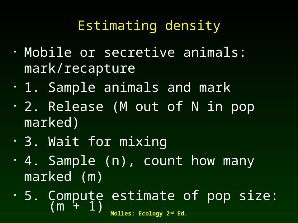
• Mobile or secretive animals: mark/recapture• 1. Sample animals and mark• 2. Release (M out of N in pop marked)• 3. Wait for mixing• 4. Sample (n), count how many marked (m)• 5. Compute estimate of pop size:

• N = M (n + 1)

(m + 1)

Molles: Ecology 2nd Ed.

• Number of animals marked in 1st sample = 100• Total number of animals in 2nd sample = 150• Number of marked animals in 2nd sample = 11

Population = M (n + 1) = 100 (151) = 1258 Size (N) (m + 1) 12

Example: Estimating Population Size from Mark-Recapture

Molles: Ecology 2nd Ed.

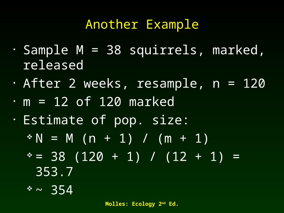
Another Example

• Sample M = 38 squirrels, marked, released• After 2 weeks, resample, n = 120• m = 12 of 120 marked• Estimate of pop. size:

N = M (n + 1) / (m + 1) = 38 (120 + 1) / (12 + 1) = 353.7 ~ 354

Molles: Ecology 2nd Ed.

Example: maple trees

• 20 randomly located plots, 10 x 10 m 20 randomly located plots, 10 x 10 m squares (area = 100 msquares (area = 100 m22))

• Average sugar maple stems per plot = 4.5Average sugar maple stems per plot = 4.5• Unit area for trees = hectare (10,000 mUnit area for trees = hectare (10,000 m22))• Density = 4.5 maples per plot / 0.01 hectare Density = 4.5 maples per plot / 0.01 hectare

plots = 450 maples / haplots = 450 maples / ha

Molles: Ecology 2nd Ed.

Example: zooplankters

• 35 lake water samples, 50 ml each35 lake water samples, 50 ml each• Average copepods per sample = 78Average copepods per sample = 78• Unit volume for zooplankton = litersUnit volume for zooplankton = liters• Sample volume = 0.05 lSample volume = 0.05 l• Density = 78 copepods per sample / 0.05 l Density = 78 copepods per sample / 0.05 l

samplessamples– = 1560 copepods / l= 1560 copepods / l

Molles: Ecology 2nd Ed.

Organism Size and Population Density

• Population density decreases with larger organism size Why? Bigger organisms need more space and

resources Bigger organisms have lower repro rates

Molles: Ecology 2nd Ed.

Damuth (1981)

• Pop density of 307 spp. of herbivorous mammals decreased with increased body size

Fig 9.19

Molles: Ecology 2nd Ed.

Peters and Wassenberg (1983)

• Aquatic invertebrates had higher pop densities than terrestrial invertebrates of similar size; mammals have higher pop densities than

birds of similar sizeFig 9.20

Molles: Ecology 2nd Ed.

Plant Size and Population Density

• Plant population density decreases with increasing plant size Underlying details different from animals

Molles: Ecology 2nd Ed.

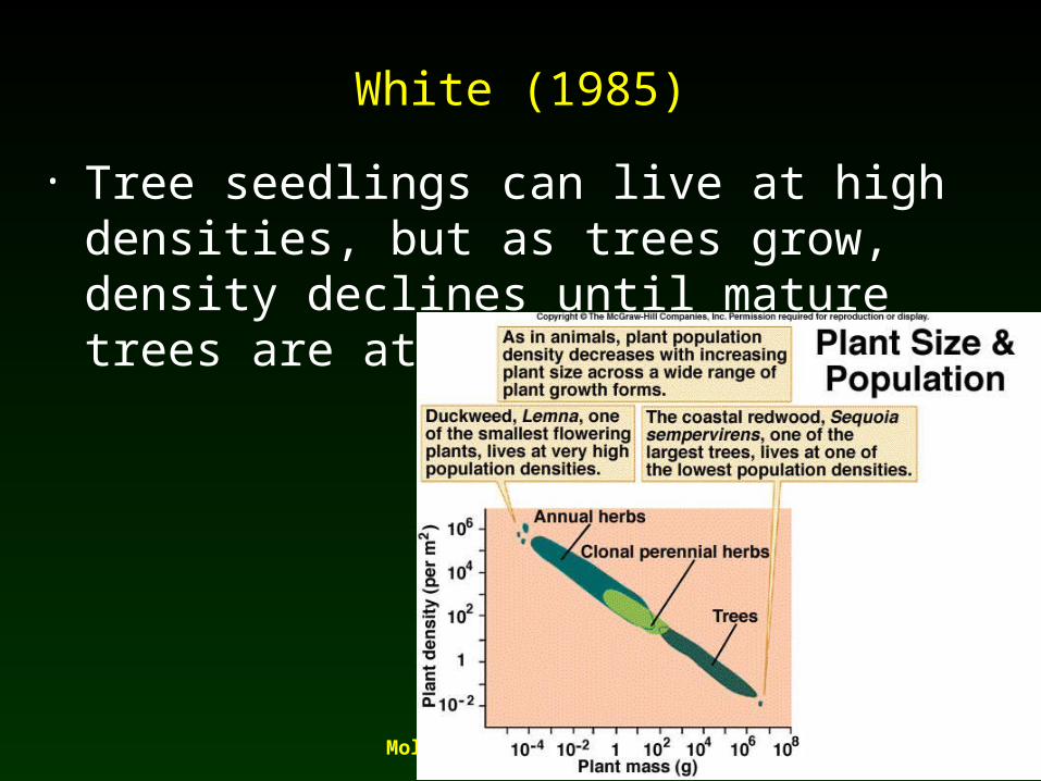
White (1985)

• Tree seedlings can live at high densities, but as trees grow, density declines until mature trees are at low densities

Molles: Ecology 2nd Ed.

Rarity and Extinction

• Rabinowitz - 7 forms of rarity• commonness classification based on (3)

factors: Geographic Range of Species Habitat Tolerance Local Population Size

Molles: Ecology 2nd Ed.

Rarity

• Non-rare populations have large geographic ranges, broad habitat tolerances, some large local populations

• All seven other other combinations create some kind of rarity

• = risk of extinction

Molles: Ecology 2nd Ed.

Rarity

• Rarity I Large Range: Broad Habitat Tolerance:

Small Local Pops Peregrine Falcons

Molles: Ecology 2nd Ed.

Rarity II

Large Range: Narrow Habitat Tolerance: Small Local Pops

Passenger Pigeons

Molles: Ecology 2nd Ed.

Rarity

• Rarity III Small Range: Narrow Habitat Tolerance:

Small Pops Mountain Gorilla

IncreasingIncreasingvulnerability tovulnerability to

extinctionextinction

IncreasingIncreasingRarityRarity

LeastLeastvulnerable tovulnerable to

extinctionextinction

ModerateModeratevulnerability tovulnerability to

extinctionextinction

HighHighvulnerability tovulnerability to

extinctionextinction

HighestHighestvulnerability tovulnerability to

extinctionextinctionOther Example ?Other Example ?

Molles: Ecology 2nd Ed.

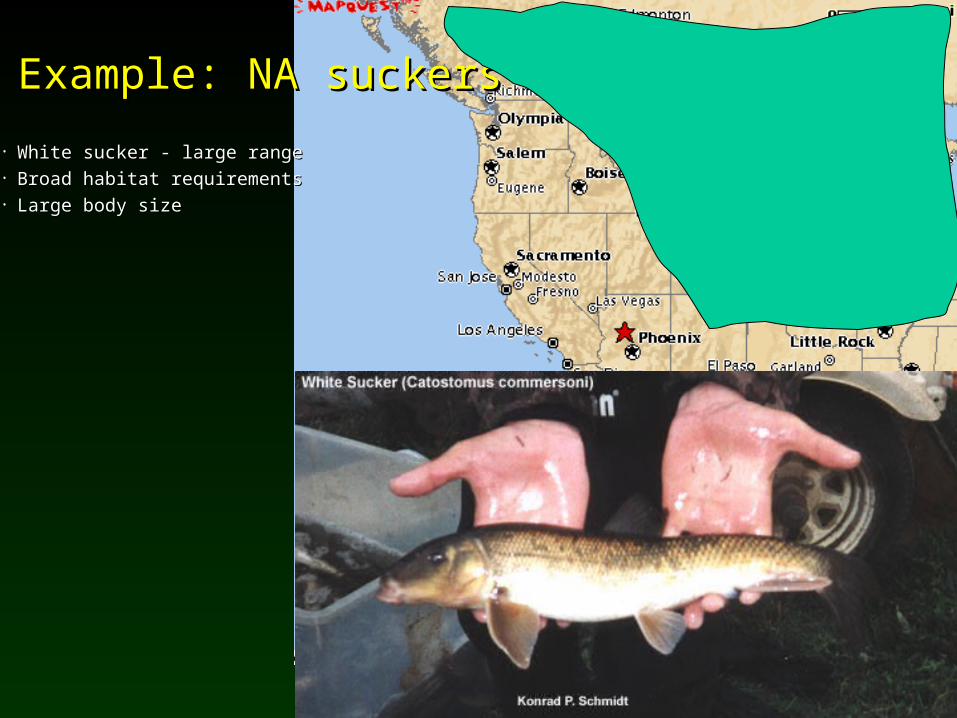
Example: NA suckersExample: NA suckers

• White sucker - large rangeWhite sucker - large range• Broad habitat requirementsBroad habitat requirements• Large body sizeLarge body size

Molles: Ecology 2nd Ed.

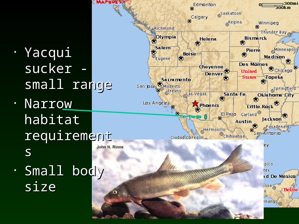
• Yacqui sucker - Yacqui sucker - small rangesmall range

• Narrow habitat Narrow habitat requirementsrequirements

• Small body sizeSmall body size

Molles: Ecology 2nd Ed.

Summary

• Physical environment limits geographic distribution of species

• On small scales, individuals w/in pops. are distributed in random, regular, or clumped patterns; on larger scales, individuals w/in pop. are clumped

• Population density declines with increasing body size

• Rarity influenced by geographic range, habitat tolerance, pop size; rare species vulnerable to extinction

Molles: Ecology 2nd Ed.