Molecular Formula Identification using High Resolution Mass ... · Methode entwickelt, um die...
127
Molecular Formula Identification using High Resolution Mass Spectrometry Algorithms and Applications in Metabolomics and Proteomics Dissertation zur Erlangung des akademischen Grades doctor rerum naturalium (Dr. rer. nat.) vorgelegt dem Rat der Fakult¨ at f¨ ur Mathematik und Informatik der Friedrich-Schiller-Universit¨ at Jena von Dipl.-Ing. Anton Pervukhin geboren am 29. Juli 1982 in Tscheljabinsk
Transcript of Molecular Formula Identification using High Resolution Mass ... · Methode entwickelt, um die...

Molecular Formula Identification using High
Resolution Mass Spectrometry
Algorithms and Applications inMetabolomics and Proteomics
Dissertation
zur Erlangung des akademischen Grades
doctor rerum naturalium (Dr. rer. nat.)
vorgelegt dem Rat der Fakultat fur Mathematik und Informatik
der Friedrich-Schiller-Universitat Jena
von Dipl.-Ing. Anton Pervukhin
geboren am 29. Juli 1982 in Tscheljabinsk
Gutachter:
1. Prof. Dr. Sebastian Bocker, Friedrich-Schiller-Universitat Jena
2. Prof. Dr. Jens Stoye, Universitat Bielefeld
Tag der offentlichen Verteidigung: 8. Dezember 2009
Gedruckt auf alterungsbestandigem Papier nach DIN-ISO 9706

Zusammenfassung
Wir untersuchen mehrere theoretische und praktische Aspekte der Identifikation derSummenformel von Biomolekulen mit Hilfe von hochauflosender Massenspektrometrie.
Durch die letzten Forschritte in der Instrumentation ist die Massenspektrometrie (MS)zur einen der Schlusseltechnologien fur die Analyse von Biomolekulen in der Proteomikund Metabolomik geworden. Sie misst die Massen der Molekule in der Probe mit ho-her Genauigkeit, und ist fur die Messdatenerfassung im Hochdurchsatz gut geeignet.Eine der Kernaufgaben in der MS-basierten Proteomik und Metabolomik ist die Iden-tifikation der Molekule in der Probe. In der Metabolomik unterliegen Metaboliten derStrukturaufklarung, beginnend bei der Summenformel eines Molekuls, d.h. der An-zahl der Atome jedes Elements. Dies ist der entscheidende Schritt in der Identifika-tion eines unbekannten Metabolits, da die festgelegte Formel die Anzahl der moglichenMolekulstrukturen auf eine viel kleinere Menge reduziert, die mit Methoden der automa-tischen Strukturaufklarung weiter analysiert werden kann. Nach der Vorverarbeitung istdie Ausgabe eines Massenspektrometers eine Liste von Peaks, die den Molekulmassenund deren Intensitaten, d.h. der Anzahl der Molekule mit einer bestimmten Masse,entspricht. Im Prinzip konnen die Summenformel kleiner Molekule nur mit prazisenMassen identifiziert werden. Allerdings wurde festgestellt, dass aufgrund der hohenAnzahl der chemisch legitimer Formeln in oberen Massenbereich eine exzellente Massen-genaugkeit alleine fur die Identifikation nicht genugt. Hochauflosende MS erlaubt dieBestimmung der Molekulmassen und Intensitaten mit hervorragender Genauigkeit.
In dieser Arbeit entwickeln wir mehrere Algorithmen und Anwendungen, die dieseInformation zur Identifikation der Summenformel der Biomolekulen anwenden. Im er-sten Teil stellen wir einen Ansatz zur Bestimmung der Summenformel eines Metabolitsdurch seine Masse und die naturliche Verteilung seiner Isotopen vor. Wir fuhren denBegriff “Isotopenmuster” ein und zeigen die Methoden fur dessen schnelle Berechnung.Wir evaluieren unseren Algorithmus auf mehreren experimentellen Datensatzen und er-reichen vielversprechende Ergebnisse mit geringem Fehleranteil fur die Molekule unter1 000 Da fur orthogonale Flugzeitmassenspektrometrie. Des Weiteren haben wir eineMethode entwickelt, um die Aminosauresequenz eines unbekanntes Proteins aus seinerSummenformel sich herzuleiten. Wir formulieren das Problem als mehrdimensionalesEquality-Constrained-Integer-Knapsack-Problem, und prasentieren effiziente Methodender Maßreduktion, um alle Problemlosungen aufzuzahlen.
Im zweiten Teil entwickeln wir mehrere Anwendungen, die unsere algorithmischenAnsatze implementieren und fur die Analyse der MS-Daten kleiner Biomolekule ange-wandt werden konnen. Wir prasentieren Decomp, eine web-basierte Anwendung furdie Massenzerlegung uber einen beliebigen Alphabet, und zeigen ihre Anwendbarkeit alsTeil eines Software-Werkzeuges CompNovo fur die de-novo-Sequenzierung von Peptiden
iii

iv
durch Tandem-MS. Schließlich stellen wir die Java-basierte Software SIRIUS vor, die un-sere Algorithmen zur Identifikation der Summenformel von Metaboliten implementiert,und mit einer leicht bedienbaren graphischen Benutzeroberflache kombiniert.

Acknowledgements
This work would not have been possible without the support of many people.
First of all, I would like to thank Prof. Dr. Sebastian Bocker, who has been a greatsupervisor over these years, sharing lots of ideas, providing dozens of useful insightsinto problems, dedicating much time for his students, and simply supporting them atall levels. For me, working with Sebastian has been an incomparable and very valuableexperience. Also, I would like to thank Prof. Dr. Jens Stoye at Bielefeld University, whohas been for me an example of a brilliant organizer and supportive mentor. Workingwith Jens in the group Genome Informatics in Bielefeld, I could particularly appreciatethe opportunity to study in a motivated and yet very friendly atmosphere, in whichthings were getting managed as if by themselves.
I am grateful to the Deutsche Forschungsgemeinschaft (DFG), which has financed mewithin the Computer Science Action Program (BO 1910/1).
I would like to express my gratitude to Dr. Michael Jung from the bj-diagnostik GmbH,Gießen, for his kindness and immense support over the period of time before beginningthis PhD thesis.
I wish to acknowledge Dr. Dirk Evers, Silke Kolsch, and the whole International NRWGraduate School in Bioinformatics and Genome Research, where I had an opportunityto study during the first one and a half years at Bielefeld University.
I express many thanks to Dr. Hans-Michael Kaltenbach who has been a great officemate in Bielefeld. I am also grateful to Dr. Zsuzsanna Liptak, who has been a greatco-author and, in some sense, an elder tutor for me in my first publications. I have beenlearning from Zsuzsa how to write clear and well-formulated papers with grammaticallycorrect English. I thank Marcel Martin, Henner Sudek, and Matthias Steinrucken whohelped me a lot in getting acquainted with realities of studying at Bielefeld University.I also wish to thank Heike Samuel for her kindness and support during my first days atmy first German university.
For the very useful and successful cooperation, I wish to acknowledge the followingscientists: Dr. Matthias Letzel at Bielefeld University, Dr. Steffen Neumann at LeibnizInstitute of Plant Biochemistry (IPB) Halle, and Andreas Bertsch at Tubingen Uni-versity. I wish to thank Henning Mersch and Jan Kruger for their help with installingDecomp at the Bielefeld University Bioinformatics Server (BiBiServ).
As during this PhD thesis, I had to change the location of my study, I would like tothank Nicole Hinz, Frank Maurer, and Anke Truß who helped me a lot to easily changethe university, and to continue research at Friedrich-Schiller-University Jena.
In particular, I would like to thank my office neighbor Thasso Griebel, who joined ournewly created group at Jena University. I feel myself lucky that he landed at my office,
v

vi
so that we could share a lot of ideas and have many useful discussions, in particular,regarding the software design and development. Without his support in the initial stageof creating SIRIUS, its release would have been much more complicated matter. I thankFlorian Rasche who came recently and could quickly adopt himself in our group, andhe is going to take over in the further development and maintenance of SIRIUS. I alsothank Martin Engler and Franzisca Hufsky for their help with SIRIUS.
I wish to acknowledge Frank Maurer for his help in correcting student assignments, andAnke Truß and Quang Bao Anh Bui for being great coworkers in holding various exercisesand seminars for students. And special thanks to Kathrin Schwotka, our beautifulsecretary, for her kindness and patience in helping us to get done all administrativeduties that typically accompany the academic research.
I thank Malte Brinkmeyer, Thasso Griebel, Florian Rasche, and Anke Truß for proof-reading parts of this thesis.
Finally, I would like to thank my parents, Gennady and Zareen, and my sister Vedanta,who have accepted my long term leaves, and eventual move to Germany. I am deeplygrateful to them for their love and support, whenever being necessary.

Contents
1 Introduction 1
1.1 Structure of the Thesis . . . . . . . . . . . . . . . . . . . . . . . . . . . . . 2
2 Biological Background 5
2.1 Atoms and Molecules . . . . . . . . . . . . . . . . . . . . . . . . . . . . . . 52.2 Proteomics . . . . . . . . . . . . . . . . . . . . . . . . . . . . . . . . . . . 82.3 Metabolomics . . . . . . . . . . . . . . . . . . . . . . . . . . . . . . . . . . 112.4 Mass Spectrometry . . . . . . . . . . . . . . . . . . . . . . . . . . . . . . . 12
2.4.1 Instrumentation . . . . . . . . . . . . . . . . . . . . . . . . . . . . 122.4.2 Experimental Workflow . . . . . . . . . . . . . . . . . . . . . . . . 18
2.5 Mass Spectrometry Data Analysis . . . . . . . . . . . . . . . . . . . . . . 212.5.1 Types of Mass Spectrometric Analysis . . . . . . . . . . . . . . . . 212.5.2 Computational Problems . . . . . . . . . . . . . . . . . . . . . . . 222.5.3 Protein Identification using Databases . . . . . . . . . . . . . . . . 24
3 Decomposition Algorithms 27
3.1 Integer Mass Decomposition . . . . . . . . . . . . . . . . . . . . . . . . . . 273.1.1 Definitions and Problems . . . . . . . . . . . . . . . . . . . . . . . 273.1.2 Enumerating Integer Decompositions . . . . . . . . . . . . . . . . . 29
3.2 Decomposing Real-valued Masses . . . . . . . . . . . . . . . . . . . . . . . 313.2.1 Approximating Number of Decompositions . . . . . . . . . . . . . 33
4 Molecular Formula Identification of Metabolites 37
4.1 Isotope Patterns . . . . . . . . . . . . . . . . . . . . . . . . . . . . . . . . 384.1.1 Isotope Species . . . . . . . . . . . . . . . . . . . . . . . . . . . . . 384.1.2 Isotopic Distributions . . . . . . . . . . . . . . . . . . . . . . . . . 39
4.2 Computing Isotope Patterns . . . . . . . . . . . . . . . . . . . . . . . . . . 414.2.1 Folding Isotopic Distributions . . . . . . . . . . . . . . . . . . . . . 414.2.2 Folding Peak Masses . . . . . . . . . . . . . . . . . . . . . . . . . . 42
4.3 Scoring Candidate Molecules . . . . . . . . . . . . . . . . . . . . . . . . . 444.3.1 Estimating Probabilities of Peak Masses . . . . . . . . . . . . . . . 454.3.2 Estimating Probabilities of Peak Intensities . . . . . . . . . . . . . 46
4.4 Experimental Results . . . . . . . . . . . . . . . . . . . . . . . . . . . . . . 464.4.1 Identification Rates . . . . . . . . . . . . . . . . . . . . . . . . . . 48
vii

viii Contents
5 Deriving Peptide Compositions 535.1 Peptide Molecular Formula Decomposition Problem . . . . . . . . . . . . 54
5.1.1 Related Problems and Solutions . . . . . . . . . . . . . . . . . . . 555.1.2 Multi-dimensional Integer Knapsack . . . . . . . . . . . . . . . . . 57
5.2 Generating Decomposition Matrices and a Mixed Matrix Approach . . . . 595.3 Experimental Results . . . . . . . . . . . . . . . . . . . . . . . . . . . . . . 60
5.3.1 Selecting Good Decomposition Matrices . . . . . . . . . . . . . . . 605.3.2 Comparison with Other Methods . . . . . . . . . . . . . . . . . . . 61
5.4 Summary . . . . . . . . . . . . . . . . . . . . . . . . . . . . . . . . . . . . 625.5 Best Six Matrix Pairs . . . . . . . . . . . . . . . . . . . . . . . . . . . . . 63
6 Application Tools and Cases 716.1 DECOMP . . . . . . . . . . . . . . . . . . . . . . . . . . . . . . . . . . . . 71
6.1.1 Introduction . . . . . . . . . . . . . . . . . . . . . . . . . . . . . . 716.1.2 Implementation and Use . . . . . . . . . . . . . . . . . . . . . . . . 72
6.2 Application Case with CompNovo . . . . . . . . . . . . . . . . . . . . . . 756.2.1 Existing Approaches for De Novo Peptide Sequencing by Tandem
MS . . . . . . . . . . . . . . . . . . . . . . . . . . . . . . . . . . . . 776.2.2 Algorithm Overview . . . . . . . . . . . . . . . . . . . . . . . . . . 796.2.3 Experimental Results . . . . . . . . . . . . . . . . . . . . . . . . . 82
6.3 Rdisop . . . . . . . . . . . . . . . . . . . . . . . . . . . . . . . . . . . . . . 846.3.1 Introduction . . . . . . . . . . . . . . . . . . . . . . . . . . . . . . 846.3.2 Implementation and Use . . . . . . . . . . . . . . . . . . . . . . . . 85
7 SIRIUS 917.1 System Architecture . . . . . . . . . . . . . . . . . . . . . . . . . . . . . . 92
7.1.1 Domain Objects . . . . . . . . . . . . . . . . . . . . . . . . . . . . 927.1.2 Functional Logic Layer . . . . . . . . . . . . . . . . . . . . . . . . . 947.1.3 Presentation Layer . . . . . . . . . . . . . . . . . . . . . . . . . . . 96
7.2 Application Workflow . . . . . . . . . . . . . . . . . . . . . . . . . . . . . 987.2.1 Preparing Input Data . . . . . . . . . . . . . . . . . . . . . . . . . 987.2.2 Analysis Preparation and Parameter Input . . . . . . . . . . . . . 997.2.3 Analyzing Algorithm Results . . . . . . . . . . . . . . . . . . . . . 101
7.3 Summary . . . . . . . . . . . . . . . . . . . . . . . . . . . . . . . . . . . . 103
8 Conclusion 105

1 Introduction
The process of scientific discovery is, in effect,a continual flight from wonder.
Albert Einstein (1879-1955)
All life on this planet basically depends on three types of molecules: DNA, RNA,and proteins. In macroscopic terms, one could visualize a cell roughly analogous to theuniversity library, where DNA are the book shelves holding all information about howthe cell works, RNA are the librarians who transfer books, small pieces of this knowledgeto students representing proteins that perform the actual tasks of the cell. In fact, this israther an oversimplified view: There exist other types of molecules, such as metabolitesthat play a crucial role in maintaining the cell’s structure as well as in the cell growth.
The sequencing of numerous genomes1 in the last two decades has stimulated im-pressive advances in the biological sciences, but emphasized our limited understandingabout the “building blocks” of biological systems. The post-genomic era has progressedby shifting the focus of bioinformatics research from structural towards functional ge-nomics: attention has grown to products of the later steps of protein expression and gen-eral functioning of the cell. For a better understanding of the biochemical and biologicalmechanisms in complex systems, it is necessary to comprehend an organism’s responseto a conditional perturbation at the transcriptome, proteome and metabolome levels.The respective areas are referred to as transcriptomics, proteomics, and metabolomics,while the eventual goal of interpretation of the whole system with its complexities isreferred to as systems biology.
Mass spectrometry has been one of the workhorse analytical tools over the last quar-ter century. Mass spectrometers are extensively used by pharmaceutical companies toanalyze small and thermostable compounds for drug research. With rapid advances ininstrumentation and capability to perform high-throughput analysis, mass spectrometryhas advanced by leaps and bounds and become a central analytical technique for proteinand metabolite research and for the study of biomolecules in general.
One of the key challenges in mass spectrometry-based proteomics and metabolomicsis to establish the identity of sample molecules. In metabolomics each individual com-pound (metabolite) needs to undergo structural elucidation, starting from the elementalcomposition or molecular formula, i.e., the number of atoms of each element. This isan essential step in identifying a metabolite, since a fixed formula reduces the numberof possible molecular structures to a much smaller set that can be further examined forautomatic structure elucidation of molecules. After preprocessing, the output of a mass
1http://www.genomenewsnetwork.org
1

2 1. Introduction
spectrometer is a list of peaks which corresponds to the masses of the sample moleculesand their abundances, i.e., the amount of sample compounds with a certain mass. Inprinciple, molecular formulas of small molecules can be identified using only accuratemasses. However, due to many chemically possible formulas in higher mass regions, ithas become evident that excellent mass accuracy alone is insufficient for the identificationpurposes.
High resolution mass spectrometry allows us to determine the isotope pattern of sam-ple molecules with outstanding accuracy. In this work, we develop several algorithmsthat extensively make use of this information for the identification of the molecular for-mula of sample molecules. To achieve this, we use and extend recently developed efficienttechniques for decomposition of integer and real-valued masses. We present a web-basedtool DECOMP for solving integer and real-valued mass decomposition problems overany arbitrary alphabet including several common “bioalphabets”, such as amino acids,nucleotides, and chemical elements most frequently occurring in nature. We demonstratethe applicability of our decomposition approach for de novo sequencing of peptides usingtandem mass spectra. Moreover, we present a novel algorithm to go one step further anduse the information about the molecular formula to derive the amino acid sequence ofan unknown peptide. To generate all amino acid sequences from a peptide’s molecularformula, our method efficiently solves a joint decomposition of a set of queries on thenumber of elements that each amino acid consists of. The performance of our approachhas been evaluated on both simulated and real proteomics data. Furthermore, we intro-duce Rdisop, a new R package for de novo identification of molecular formulas solely frommasses and isotope patterns measured by high resolution mass spectrometers. Finally,we present the java-based software application, called SIRIUS, that implements all ofour algorithms for identification of the molecular formula of metabolites, and combinesthem with an easy-to-use graphical user interface.
Parts of this dissertation thesis have been published in advance [15, 17, 16, 20], andone further paper is accepted for publication [12]. Decomp is freely accessible at theBielefeld University Bioinformatics Server2 (BiBiServ). Rdisop is distributed as a partof the Bioconductor project, and is publicly accessible at the project website3. SIRIUSis publicly available for download at the project website4, and is distributed for variousoperating systems including Unix/Linux, Windows and Mac OS.
1.1 Structure of the Thesis
This thesis consists of eight chapters. In Chapter 2, an introduction into the basic termsand principles in computational molecular biology, in particular, the emerging fieldsof proteomics and metabolomics, is given. We introduce mass spectrometry (MS) andits biotechnological aspects, and outline the computational problems that arise in itscontext.
2http://bibiserv.techfak.uni-bielefeld.de/decomp/3http://www.bioconductor.org/packages/2.4/bioc/html/Rdisop.html4http://bio.informatik.uni-jena.de/sirius/

1.1 Structure of the Thesis 3
The thesis is organized as follows: The first part (Chapters 3–5) is devoted to thetheoretical concepts of our research. In Chapter 3, we start by a brief detour to existingapproaches for decomposing integer masses, a question that is frequently encountered inthe MS data analysis. We define the relevant problems and introduce available computa-tional solutions, which are further used as a basis in all our algorithms and applications.We also show how to extend the integer decomposition techniques for the analysis ofreal-valued MS data.
Chapter 4 presents a new approach for de novo identification of molecular formulas ofmetabolites, which uses the mass decomposition techniques, and incorporates further in-formation, such as isotopic abundance data. We introduce an isotope pattern and relatednotions, and present methods for the fast simulation of isotope patterns, which is im-portant for the analysis of larger molecules where the search space increases rapidly. Weevaluate our approach on several experimental datasets using different MS techniques,and obtain very promising results with only a tiny proportion of false identifications formolecules below 1 000 Da for orthogonal time-of-flight mass spectrometry.
In Chapter 5, we present a new algorithm that employs the molecular formula in-formation to efficiently infer the amino acid composition of an unknown peptide. Weformulate the problem as a joint set of decomposition queries based on the number ofelements that each amino acid consists of, and present a dimension reduction techniqueto reduce a multi-dimensional problem to a one-dimensional instance. We also providean experimental evaluation of the algorithm performance, both on simulated data andpeptides from experimental mass spectra.
The second part (Chapters 6 and 7) is devoted to the practical aspects of our work.In Chapter 6, we present several application tools that implement our algorithmic ap-proaches, and can be utilized for the MS data analysis of small sample molecules. Wepresent Decomp, a web-based application to find decompositions of a given mass overany arbitrary alphabet. Being designed to solve integer and real-valued mass decompo-sition problems, Decomp is well suited both for the interpretation of MS data and forsolving instances of Money Changing Problem. We then demonstrate its applicability asan essential part of another algorithm, called CompNovo, for de novo peptide sequenc-ing using tandem mass spectrometry. We also present Rdisop, a new R package for theanalysis of small sample molecules using an accurate isotope pattern information.
In Chapter 7, we present the java-based software SIRIUS with the implementation ofall our algorithms for de novo identification of molecular formula of metabolites usinghigh resolution MS data. We describe the architecture and provide some technical detailson implementations and employed technologies. Well-defined structure and managementsystem of our software allow a simple integration of new computation and visualizationfunctionalities to the application. We further describe a basic application workflow andoutline the cornerstones of the data and analysis preparation. We discuss a set of SIRIUSfeatures for the interpretation of the computational results including visualization, dataexport, and searching for molecular formulas in biological databases.
Chapter 8 concludes the thesis by recalling the main results and presenting an out-look on further applications of the molecular formula analysis for the identification ofunknown sample molecules.


2 Biological Background
We start by providing some basic physical and chemical background, which we furtheruse throughout this work. Since the motivation of our work as well as its applicationsand results have their origin in proteomics and metabolomics, this chapter will give anoverview of the central terms and principles of these two emerging fields of scientificresearch. Main focus of our work also lies in the context of mass spectrometry, thus wewill briefly describe the basics of mass spectrometry, and outline the computational chal-lenges that appear in its context. This chapter cannot be a self-contained introductionto mass spectrometry or to the fields of proteomics and metabolomics, and for furtherinformation, the interested reader might have a look at any of the relevant textbooks,e.g., [57, 34,125].
2.1 Atoms and Molecules
Atoms and Isotopes. The word “atom” comes from the Greek word atomos, whichmeans uncuttable: Atoms are basic units of matter that cannot be decomposed chem-ically. Atoms consist of a central nucleus surrounded by negatively charged electrons.The atomic nucleus is made up from positively charged protons and neutrons which haveno charge. Atoms contain the same number of protons and electrons, and thus have nocharge; if this charge is broken, the resulting particle is called an ion.
Atoms are classified according to the number of protons and neutrons in their nucleus.The total number of protons and neutrons is called the nominal mass, or the nucleonnumber of an atom. The number of protons is referred to as the atomic number anddetermines the chemical element of an atom. Atoms with equal atomic numbers sharethe same chemical behavior and cannot be distinguished chemically. The elements mostabundant in living beings are hydrogen (symbol H) with atomic number 1, carbon (C,atomic number 6), nitrogen (N, 7), oxygen (O, 8), and to lesser extent, phosphor (P, 15),and sulfur (S, 16). Throughout this work, we will refer to this set as CHNOPS.
Unlike the fixed number of protons, the number of neutrons of an element can vary:Atoms with equal number of protons and electrons but different number of neutronsdefine the isotopes of an element. For example, carbon has two isotopes that occurin nature, 12C and 13C (the preceding superscript denotes the nucleon number): 12C iscomprised of six protons, six electrons, and six neutrons, whereas 13C carries six protons,six electrons, and seven neutrons.1 The lightest isotope, such as 1H or 12C, is also calledmonoisotopic. Note that the term “monoisotopic” is sometimes referred to as the most
1In fact, carbon has the third radioactive isotope 14C. Radioactive isotopes are usually ignored in massspectrometric analysis.
5

6 2. Biological Background
element (symbol) isotope abundance % mass (Da) av. mass (Da)
hydrogen (H) 1H 99.985 1.0078252H 0.015 2.014102 1.007976
carbon (C) 12C 98.890 12.013C 1.110 13.003355 12.011137
nitrogen (N) 14N 99.634 14.00307415N 0.366 15.001090 14.006727
oxygen (O) 16O 99.762 15.99491517O 0.038 16.99913118O 0.200 17.999160 15.999305
phosphor (P) 31P 100 30.973762 30.973762sulfur (S) 32S 95.020 31.972071
33S 0.750 32.97145934S 4.210 33.96786736S 0.020 35.967081 32.064388
proton (p+, 1H+) 1.00728 Da, neutron (n) 1.008665 Da, electron (e – ) 0.00054 Da
Table 2.1: Natural isotopic distribution: Relative abundance of isotopes and their massesin Dalton.
abundant isotope, but in this work we use this term to refer to the isotope with thesmallest mass. Isotopes of each element are found in nature with certain abundance:For example, the relative abundance of the monoisotopic carbon isotope 12C is 98.89 %,whereas the isotope 13C has the relative abundance of 1.11 %. For abundances of otherisotopes most commonly occurring in nature, see Table 2.1.
Masses of atoms are measured in Dalton (Da), or equivalently in unified atomic weightunits (u). According to International Union of Pure and Applied Chemistry (IUPAC),one Dalton is defined as 1/12 of the mass of one atom of the 12C isotope. In fact, dueto the mass contained in the binding energy of the atom’s nucleus, an atom with nprotons and neutrons has a mass, which roughly, but not exactly, equals to n Da. Thisillustrates the mass defect, the difference between the atom’s nominal mass and the sumof masses of the constituting protons, neutrons, and electrons. For example, the totalmass of 6 protons, 6 neutrons, and 6 electrons is equal to 12.09596 Da, while the 12Cisotope has a mass of exactly 12.0 Da, a difference of about 0.8 %. The average mass ofan element is the expected mass computed with respect to the relative abundances ofisotopes. For example, the average mass of carbon is 0.98890 times the mass of 12C plus0.01110 times the mass of 13C. For the masses of elements listed above, see Table 2.1,while the detailed list of all chemical elements can be found in [4].
Molecules. A molecule is a stable group of two or more atoms joined together bychemical bonds of shared pairs of electrons. A molecular formula indicates the exact

2.1 Atoms and Molecules 7
number of atoms that compose a molecule. Compared to the chemical formula that mayprovide information about the structure and types of chemical bonds, the molecularformula only reflects the amount of atoms in the molecule. For example, the chemicalformula of the amino acid alanine CH3CH(NH2)COOH implies a chain of three carbonatoms, with an α-carbon (see Section 2.2) surrounded by an amino group (NH2), acarboxyl group (COOH), and a methyl group (CH3), whereas the molecular formulaC3H7NO2 tells us only that the molecule contains 3 carbons, 7 hydrogens, 1 nitrogen,and 2 oxygens. Molecules can have different amount of protons and electrons, thus beingpositively or negatively charged. Molecules that pick up a net electric charge are calledions, or in the context of mass spectrometry, they are often referred to as molecular ionadducts.
Chemical Bonding Rules. Atoms in the molecule are held together by the chemicalbonds formed through the pairs of electrons that atoms can share with their neighbours.The number of chemical bonds formed by atoms is often referred to as the valence ofan element. For example, in natural compounds carbon has valence 4, oxygen 2, andhydrogen 1. However, for many elements, the valence varies depending on the moleculeto which this element belongs. For example, phosphor sometimes forms 5 chemical bondsand sometimes only 3. For the physical existence of a molecule as a set of interconnectedelements, certain chemical rules, such as a valence balance and unsaturation, must hold.In its stable state, the molecule is an electrically neutral entity with the same numberof protons and electrons. Therefore, the valence states of all its constituting atoms mustbe balanced. For example, if one atom would have valence +1, meaning it lacks oneelectron, and another atom would have valence −1, meaning it possesses an additionalelectron, then a bond between these two atoms would be formed to complement theirunbalanced valence states.
Another prerequisite of the legitimate compound is the number and types of bondsthat must be present. A molecule only containing single bonds is called saturated, whilethe presence of multiple bonds is known as unsaturation. The degree of unsaturation(DU) [96] formula, also known as rings-plus-double-bonds equivalent (RDBE) [114], helpsto determine the number of different types of bonds in the compound, and therefore canbe used for validation of molecular formulas.
In 1951, Senior [107] proposed a graph-theoretical concept to unify the aspects ofvalence balance and unsaturation. Senior’s theorem outlines the three prerequisites forthe existence of a molecular graph:
1. The sum of valences or the total number of atoms having odd valences is even;
2. The sum of valences is greater than or equal to twice the maximum valence;
3. The sum of valences is greater than or equal to twice the number of atoms minusone.
The first condition corresponds to the valence balance, whereas the third conditionaccounts for connectivity of a molecular graph requiring the number of independent

8 2. Biological Background
cycles in the graph to be nonnegative. The second prerequisite ensures the non-existenceof small molecules such as CH2.
There exist other chemical criteria, such as a nitrogen rule, or a Lewis octet rule, butthey are either rarely used for mass spectrometric analysis, or can be seen as a subsetof Senior’s conditions.
2.2 Proteomics
The word “proteome” was coined in 1994 to denote the total amount of PROTEinsexpressed by a genOME, cell, tissue or organism [91]. More specifically, it is the set ofexpressed proteins at a given time under defined conditions. Unlike the genome, theproteome is very dynamic: Proteins are constantly formed and degraded in different celltypes and their expression is influenced by the environment and events going on insidethe cell, such as cell division and growth state. Proteins participate in almost all cellularprocesses: They are part of the cell membrane, form enzymes that perform biochemicalreactions, and serve as receptors and transmitters in signal transduction. Identificationof all the proteins in a cell or an organism is one of the major tasks of proteomics – thestudy of the proteome.
Protein Structure. Proteins are polypeptides: They form a chain of amino acid mole-cules linked together in a certain order by peptide bonds.
There are 20 different naturally occurring amino acids, all sharing the same commonstructure: A central carbon atom (often denoted by α (alpha) carbon) surrounded byan amino group (HN2), a carboxyl group (COOH), a hydrogen atom and a side chainspecific for the amino acid. The generalized structure of an amino acid is depicted inFigure 2.1. Each amino acid can be denoted either by its full name, symbol, or three-letter abbreviation, see Table 2.2. Note that leucine (L) and isoleucine (I) have identicalmolecular formula and usually cannot be distinguished by mass spectrometry. In thefollowing, we thus consider these two amino acids as one, and talk about 19 standardamino acids.
From the structure shown in Figure 2.1, it is obvious that an amino acid looses awater molecule (H2O) when it is included in the chain. Therefore, when amino acidsare part of a chain, they are commonly referred to as residues. The bonds betweentwo consecutive amino acid residues in the chain are amide bonds, and are denoted aspeptide bonds. Correspondingly, a short chain of amino acids is usually referred to as apeptide. Each peptide has an an unbounded amine group, called the N-terminus, and anunbounded carboxyl group, called the C-terminus. By convention, the peptide sequenceis written as a string of residues (usually denoted by symbols) from the N-terminus tothe C-terminus.
The peptide sequence is the most fundamental attribute of a protein and thereforereferred to as its primary structure: If the sequence is known, the protein is consideredidentified. To determine the complete peptide sequence is, however, not a straightforwardprocess.

2.2 Proteomics 9
Cα
R OH
CH
O
NCα
R
H
CH
O
Cα
HN
H
C
R
O
N
H
Cα
R
CH
OH
H
Residues
H Cα
HN
H
C
R
O
OH N
Amino group Carboxyl group
Side chain
N-terminus C-terminus
a) b)
Peptide bond
Figure 2.1: a) All amino acids have the same common structure. Different amino acidsvary in their side chains. b) A polypeptide is formed by linking togethermultiple amino acids residues.
Protein Synthesis. In modern molecular biology, the word “genome” refers to thehereditary information of an organism encoded in several deoxyribonucleic acid (DNA)molecules, each a double-stranded polymer built from four different nucleic acids, or nu-cleotides: adenine (symbol A), cytosine (C), guanine (G) and thymine (T). The genomeis mainly static and the same for all cells of an organism. The primary structure of aprotein is encoded in a gene, a coding region of the genome.
Protein synthesis is the creation of proteins using DNA and ribonucleic acid (RNA)molecules. RNA molecules are very similar to DNA molecules, except that they aresingle-stranded, use a different ribose in the backbone and have the base uracil (U)instead of thymine (T). To build a new protein, the gene that encodes this proteinmust be transcribed and translated. During the transcription, messenger ribonucleicacid (mRNA) molecules are formed that contain a complementary copy of the geneticinformation. Similar to the genome and the proteome, the transcriptome is the set of allmRNA molecules present in a cell at a certain time. Like the proteome, the transcriptomeis dynamic.
In the translation process, the mRNA molecules, containing the genetic instructionsto make the protein, are first brought to the ribosomes, large ribonucleoproteins that areresponsible for building the protein’s primary structure from amino acids. This processis done with the help of transfer RNA (tRNA) that transfers the amino acids to theamino acid chain. The actual translation is done by the ribosomes that read the mRNAsequence of nucleic acids and for each triplet of nucleotides, or codon, add the encodedamino acid to the so far formed amino acid chain. Codons are consecutive and non-overlapping, that is the next triple of nucleotides after each codon corresponds to thenext codon. The start and the end of the translation process are triggered by specialstart and stop codons. When the ribosome reaches the stop codon, indicating the endof the mRNA sequence, it releases the protein that then folds to its final structure.
This flow of information in a cell,
DNA → transcription → RNA → translation → protein

10 2. Biological Background
amino acid symb. TLC molecular mass (Da)formula mono. average
Alanine A Ala C3H5N1O1 71.0371 71.0788Cysteine C Cys C3H5N1O1S1 103.0091 103.1448Aspartic acid D Asp C4H5N1O3 115.0269 115.0886Glutamic acid E Glu C5H7N1O3 129.0425 129.1155Phenylalanine F Phe C9H9N1O1 147.0684 147.1766Glycine G Gly C2H3N1O1 57.0214 57.0520Histidine H His C6H7N3O1 137.0589 137.1412Isoleucine I Ile C6H11N1O1 113.0840 113.1595Lysine K Lys C6H12N2O1 128.0949 128.1742Leucine L Leu C6H11N1O1 113.0840 113.1595Methionine M Met C5H9N1O1S1 131.0404 131.1986Asparagine N Asn C4H6N2O2 114.0429 114.1039Proline P Pro C5H7N1O1 97.0527 97.1167Glutamine Q Gln C5H8N2O2 87.0320 87.0782Arginine R Arg C6H12N4O1 156.1011 156.1876Serine S Ser C3H5N1O2 87.0320 87.0782Threonine T Thr C4H7N1O2 101.0476 101.1051Valine V Val C5H9N1O1 99.0684 99.1326Tryptophan W Trp C11H10N2O1 186.0793 186.2133Tyrosine Y Tyr C9H9N1O2 163.0633 163.1760
Table 2.2: Amino acid residues with 3-letter-code (TLC), symbol, molecular formula,monoisotopic (mono.) and average masses. The molecular formulas for theresidues are given without terminal H and OH groups.
is referred to as the central dogma of molecular biology. In fact, this is rather an oversim-plified view on the transfer of biological information in a cell: Today, we know other fac-tors, such as an alternative splicing of introns, DNA and RNA editing, post-translationalmodifications (PTM), and others, that make this process more complicated, resulting ina variability of protein molecules translated from a single gene. Here, we omit furtherdetails.
Although DNA, RNA and proteins are the main players in the cell’s life circle and thethree primary types of molecules that biologists study, there are other types of molecules,such as metabolites that play a crucial role in maintaining the cell’s structure. In thenext section, we address metabolites in more detail.

2.3 Metabolomics 11
2.3 Metabolomics
Metabolites are the end products of cellular regulatory processes, and their expressionscan be considered as the ultimate response of biological systems to genetic or environ-mental changes [42]. Metabolomics deals with the systematic study of the metabolismof both endogenous and exogenous metabolites present in biological systems. The word“metabolism” is derived from the Greek word metabole, meaning change, which is appli-cable as metabolism is in a constant and rapid flux. In analogy to genome and proteome,metabolome refers to the total amount of metabolites present in a biological system thatparticipate in metabolic reactions such as growth, maintenance and normal function [57].Metabolites are organic and inorganic species, mostly of small molecular mass. Metabo-lites are usually divided into two categories: primary metabolites are directly involvedin growth, development, or reproduction of an organism, whereas secondary metabolitesare not directly involved in these processes, but have other important biological func-tions. Endogenous metabolites are biochemically synthesized or catabolized within thecell or organism, whereas exogenous metabolites have an external origin, as is the casefor pharmaceuticals and food nutrients consumed by humans.
A typical analytical procedure in metabolomics can be divided in three major steps:First, a biological sample must be collected without causing any change of the metabolo-me: the metabolite molecules must be extracted and eventually undergo chemical deriva-tization. Second, the metabolites are separated by chromatographic techniques, such asgas chromatography (GC) or high performance liquid chromatography (HPLC), see Sec-tion 2.4. Finally, metabolites are identified and quantified using Mass Spectrometry, orNuclear Magnetic Resonance (NMR).
Although metabolomics is closest to the phenotype in the “omics” cascade (see Fig-ure 2.2), there currently exists no single-instrument platform that can analyze all metabo-lites, and the tools for the comprehensive examination of the metabolome are still emerg-ing [13]. In Table 2.3, a list of different strategies is given that are currently employed.The complexity of the metabolome is due to the broad variety of compounds, such aslipids, carbohydrates, vitamins, and others, which comprise the metabolome. Thesecompounds constitute a diverse set of molecular structures when compared to the pro-teome (string of 20 standard amino acids) and transcriptome (string of 4 nucleotides).The majority of metabolites contain only six elements CHNOPS that most frequentlyoccur in living beings. However, metabolites can also contain other elements, such aschlorine (Cl), fluorine (F), and others [72]. This results in a wide variety of chemical(molecular weight, polarity, solubility) and physical (volatile) properties of metabolitesbecoming a challenge for the comprehensive biochemical analysis.
One of the major applications of metabolomics is the detection of biomarkers thatchange as an indicator of the presence of a disease in an individual biological system. Thebiomarkers for certain diseases, such as for reversible myocardial ischemia, can be foundon metabolomic, rather than on genomic or proteomic level [103]. Also, metabolomicshas been employed in a variety of other health applications including pharmacology,pre-clinical drug trials, clinical chemistry, and others. Moreover, the concept of in-dividualized health, such as nutrition or tailored pharmacological treatment based on

12 2. Biological Background
genome
transcriptome
proteome
metabolome
phenotype
What сan happen
What appears tobe happening
What makes it happen
What has happened and is happening
Figure 2.2: The “Omics” cascade contains several levels of the biological system, whichcan be analyzed with regard to the response of the system to disease, genetic,and environmental changes. Of these levels, the metabolome is the mostpredictive of phenotype.
metabolic phenotype will strongly rely on metabolomics technology [124].
2.4 Mass Spectrometry
Mass spectrometry is an analytical technique that has played a key role in emergingof proteomics and metabolomics into mainstream science. In the remainder of thischapter, an introduction to the field of mass spectrometry from both experimental andcomputational points of view is given.
According to Siuzdak [110], a mass spectrometer is “an analytical device that deter-mines the molecular weight of chemical compounds by separating molecular ions accord-ing to their mass-to-charge (m/z) ratio”. As mentioned before, molecular weights aremeasured in Dalton (Da), or equivalently in unified atomic weight units (u). One Dal-ton equals one atomic weight unit (amu) of 1.66 · 10−24 g, which is approximately themolecular weight of one proton. The mass-to-charge is measured in Thompson (Th).
2.4.1 Instrumentation
Very schematically, a mass spectrometer consists of three main parts as shown in Fig-ure 2.3: the ionization source, the mass analyzer, and the detector. Following the sampleintroduction, the analyte is ionized in an ionization source, either operating at atmo-spheric or vacuum pressures. The generation of charged molecules is necessary to enableion manipulation based on its mass-to-charge (m/z) ratio. The sample is then trans-ferred to the mass analyzer that separates the components of the sample in space or time

2.4 Mass Spectrometry 13
Metabolomics Identification and quantification of as many of the com-pounds present in a metabolome sample as possible.
Metabolic profiling Identification and approximate quantification of a large setof metabolites, generally related by one or more specificmetabolite classes, within a metabolite sample. This strat-egy can be also described as metabolite profiling or untar-geted analysis, and provides metabolite identifications wherethe compounds of biological interest are not known a priori.
Targeted analysis Identification and precise quantification of a single or highly-related small set of metabolites within a metabolome sam-ple.
Metabolic fingerprinting High-throughput generation of a global snapshot, or fin-gerprint, of a metabolome sample without regard for theindividual compounds that it contains. Identification andquantification is limited and the strategy is employed fordiscrimination of samples from different biological origins.
Table 2.3: Typical strategies employed in metabolomic analysis.
according to their m/z ratios. After separation, ions are registered by a detector eitherphysically as an ion current or by the detection of orbital frequencies as image currents.Finally, the mass spectrometer’s output – a mass spectrum – is acquired by a connectedcomputer. A mass spectrum is a diagram, with the position of the peak along the hor-izontal axis that ideally indicates the presence of the molecule with the correspondingm/z value in the sample, and the height of the peak, referred to as intensity or relativeabundance, which is proportional to the amount of molecules with this m/z value.
Sample introduction(gas, liquid, solid)
Ion source Mass analyzer Detector PC
Figure 2.3: Schematic principle of the mass spectrometer
In the following, we briefly describe the main ionization sources and mass analyzers.A comprehensive survey with more details about instrumentation can be found in [54].

14 2. Biological Background
Ionization Sources. Although invented in the late 19th century, mass spectrometry(MS) for a long time was restricted to small and thermostable molecules due to thelack of proper techniques to “softly” ionize and transfer ionized molecules from thecondensed phase to the gas phase without excessive fragmentation. This situation waschanged in the late 1980s, with the development of two techniques for the routine andgeneral accumulation of molecular ions of entire biomolecules, namely matrix-assistedlaser desorption/ionization (MALDI) [61,68] and electrospray ionization (ESI) [39,126]that allowed the ionization of higher-value molecules such as proteins. For the develop-ments of these invaluable MS technologies, Koichi Tanaka (MALDI) and John B. Fenn(ESI) were given the Nobel Prize in Chemistry in 2002.
In MALDI, the analytes are dissolved with a matrix solution and a small drop (mi-croliter volume) is spotted on a metal plate and allowed to dry. After drying, the metalplate is transferred to the vacuum system of the mass spectrometer and a laser beamshots onto a matrix, with wave length specific to the matrix. The absorbed energy causesthe matrix to evaporate, releasing the enclosed analyte and ionizing it. The ionization istypically singly-charged protonation, meaning that the ionized molecules carry one ad-ditional proton. Finally, directed by the electric field, ionized molecules are transportedto the mass analyzer. Since only a part of the sample and the matrix is used with eachlaser shot, the same sample can be measured multiple times. Moreover, MALDI platescan be kept and re-used in later experiments, allowing interruptions in the analysis.
In ESI, the analyte is dissolved in a liquid solvent, and is sprayed from a tiny highlycharged needle or capillary into a strong electromagnetic field, resulting in a condensateof small aerosol droplets with a charged surface. The droplets are brought into thevacuum system of mass spectrometer, and as the solvent in the droplets evaporates,they get smaller and smaller, increasing the electric field on the surfaces. When theelectric field becomes strong enough, charged molecules desorb from the surfaces. Theseconditions usually result in multiply protonated ions. Finally, influenced by the electricfield, ions are brought to the mass analyzer. In contrast to MALDI, ESI relies oncontinuous supply of dissolved analytes, which makes it particular suited for couplingwith liquid chromatography, see Section 2.4.2.
Mass Analyzers and Detector. Mass analyzers separate ionized molecules, influencedby the electromagnetic field according to their m/z ratios. Varying in physical principlesand performance standards, there exist several types of mass analyzers that are employedin proteomics and metabolomics. Here, we first introduce several widely used technolo-gies. Since most of our work was performed on high resolution mass spectrometers, wethen introduce several novel techniques, employment of which is increasingly becominga routine technique in modern laboratories, that allows for a precise and comprehensiveanalysis of complex biological systems [81].
The simplest and most frequently used mass analyzers are time-of-flight (TOF) an-alyzers, quadropoles and ion traps. TOF analyzers are usually coupled with MALDI,whereas quadropoles and ion traps come along with an ESI source.
In a TOF analyzer, the ionized analyte is accelerated by an electric field for a certain

2.4 Mass Spectrometry 15
distance. Due to the same force of the electric field applied for all ions, the velocity of aparticular ion depends only on its mass and charge. Assuming the same singly-chargedtype of ions produced by MALDI, an ion’s velocity depends only on its mass. Afteracceleration, ions drift in the field-free tube towards detector. Clearly, the time neededto pass the tube depends on velocity. When a particular ion hits the detector at theend of the tube, the flight time is registered, and the mass of an ion is calculated. Theprinciple of a linear MALDI-TOF instrument is illustrated in Figure 2.4.
Matrix/sample
Laser
Ions
acceleration drift tube
Analyzer Detector
voltageM1 > M2 > M3
Figure 2.4: Illustration of a linear MALDI-TOF mass spectrometer.
Quadrupole analyzer consists of four circular metallic rods arranged parallel to eachother. Each opposite pair of rods is connected together electrically, and a high frequencyalternating voltage applied on the rods produces a high oscillating electromagnetic fieldbetween them. Ions passing through the field will move in spiral trajectories with theradius depending on the m/z value of a particular ion and on the offset voltage of the field.For a specific strength and frequency of applied voltage, only ions within a particular,very confined m/z range will reach the detector, whereas others will be deflected.
Ions traps (IT) function by a similar principle as quadrupole, but the ions are capturedin a confined space of a vacuum system or tube. Ion traps exist in both linear and 3Dform, while the latter is often referred to as a quadrupole ion trap (QIT), or Paul trap.The name is credited to its inventor Wolfgang Paul, who shared the Nobel Prize inPhysics in 1989 for this work. One can think of a QIT trap as a quadrupole with two ofthe rods forming the endcap electrodes and a third bent into the ring electrode betweenthem. Similar to quadrupole, the ions are moved by specific trajectories within the trapby applying an alternating voltage that results in an oscillating electric field inside thetrap. Applying certain voltage causes ions of a particular m/z range to be released fromthe trap; the ejected ions are subsequently recordered by the detector.
The detector is typically build as an electron multiplier, and measures the signal byconverting the kinetic energy of arriving ions into an electric current. The ion currentis registered in equal intervals of time. Since the strength of the current depends on thequantity of ions, the ion current is referred to as the intensity of that particular m/zvalue.
16 2. Biological Background
Mass Accuracy and Resolution. Experimentally measured masses, or m/z values in-evitably have some errors or uncertainties. The total error of mass measurements isgiven as either an absolute, or relative value. An absolute error is typically provided inDalton, or milli-mass unit (mmu), where 1 mmu equals 0.001 Da. A relative error iscommonly given in parts-per-million (ppm), and is also referred to as a mass accuracy.The mass accuracy of 10 ppm for measuring a molecule with mass 1 000 Da is equivalentto an absolute error of 0.01 Da.
The term mass resolution, or resolving power describes an ability of mass spectrom-eter to discriminate between several peaks with small differences in their masses. The
resolution (R) of mass m is calculated as R =m
∆m, with two common ways to determine
∆m residing in two corresponding IUPAC definitions: the ρ percent valley definition andthe peak width definition.
In the ρ percent valley definition, ∆m is defined as the smallest spacing between twoequally intense peaks with a valley between them, while the height of the valley at itslowest point is bigger than ρ percent of either peaks. The typical value for ρ is 10%.
In the peak width definition, ∆m is defined as the width of the peak at a height which isa specified portion of the maximum peak height. According to IUPAC, it is recommendedto always use one of the three values: 50 %, 5% or 0.5 %. A most common standard isto measure the full width of the peak at half of its maximum height, also abbreviated as“FWHM”. The higher values of mass resolution indicate a better separation of peaks.
Because of imperfections in ionization sources and mass analyzers, charged moleculeswith equal m/z values never reach a detector at exactly the same time. For example,in MALDI-TOF mass spectrometers the ions are not shot from exactly the same spoton the matrix, therefore being spread out in 3D space when they enter the electricfield. Thus, their velocities after acceleration may slightly differ. As a result, hitting thedetector at slightly different times, two ions with equal m/z values are registered as one“merged” peak of a certain width. This behavior consequences in worser resolution –ions of similar m/z values may not be distinguished, and in lower mass accuracy – theactual m/z value may not be detected exactly, but only with some tolerance.
Ion Cyclotron Resonance and Orbitrap Mass Analyzers. The introduction and com-mercialization of Fourier transform-ion cyclotron resonance (FT-ICR) mass spectrom-eters with external ionization sources [108] was a breakthrough in terms of the massaccuracy and resolving power of mass spectrometers, with a completely new principle todetermine the masses of charged molecules.
As its name implies, a FT-ICR analyzer is equipped with a cyclotron that acceleratescharged molecules to high energies. The cyclotron contains a Penning trap (a magneticfield with electric plates), and the ions are moving in circles around this magnetic fielddirected by an applied voltage. Under the influence of an oscillating electric field thatis placed perpendicular to the magnetic field, the ions are excited to a larger cyclotronradius. The frequency (or angular velocity) of a particular ion depends on its m/z valueand the strength of the magnetic field applied. Instead of a detector, a pair of plates isused to record a signal from ions that pass close by. Since the ions are moving in packets,

2.4 Mass Spectrometry 17
the frequencies of several ions are recorded simultaneously, resulting in a superposition ofsine waves. The frequency of a particular ion is extracted from this “interlaced” diagramby applying a Fourier transformation. With individual frequencies extracted, it is thenstraightforward to derive the corresponding m/z values.
The resolution and mass accuracy of FT-ICR analyzer are extremely high. However,its employment adds a sizeable economic burden mostly due to the costs of the super-conducting magnet.
Recently, a new type of mass analyzer, called Orbitrap [56], was introduced. Like FT-ICR, Orbitrap follows the same principle to measure the frequency of rotating ions, butinstead of a magnet, an oscillating electric field is used for the acceleration of chargedparticles.
An Orbitrap consists of an outer and inner coaxial electrode that create an electrostaticfield. The ions are injected into the field between electrodes, and influenced by centrifugalforces, start moving around the inner electrode. Additionally, the ions move back andforth forming a harmonic oscillation in orbits along the axis of the electrostatic field. Theoscillating frequency of a particular ion is inversely proportional to its m/z value. Likein FT-ICR analyzer, the m/z value of a single molecule is derived from the superpositionof sine waves of several ions by applying a Fourier transformation. Thus, an Orbitrapanalyzer provides a resolution and mass accuracy similar to FT-ICR, but saves on theusage of the expensive superconducting magnet. The design of Orbitrap analyzer ispatented by Thermo Scientific2.
The development of new mass analyzers catalyzed further improvements of instru-mentation by assembling complex multistage instruments specifically suited for variousexperimental setups. One typical example is a hybrid quadrupole time-of-flight (Q-TOF)mass spectrometer that combines a quadrupole and TOF analyzer. Employing a TOFanalyzer in the last stage allows to achieve a higher mass resolution, and fastens theanalysis, which makes this design better suited for protein and proteome analysis [3].
Tandem Mass Spectrometry. As its name implies, the principle of tandem mass spec-trometry is based on two mass analyzers in tandem. In the first mass analyzer, a partic-ular ion is selected based on its m/z ratio. In the second analyzer, the selected peptideion undergoes a fragmentation step, resulting in the fragment ions of this peptide ion. Inthe second analyzer, masses of the fragment ions are recorded. The spectrum containingmeasured m/z values and intensities of the fragment ions is called an MS/MS spectrum,or product ion spectrum. The peptide ion selected for fragmentation is referred to as aprecursor ion, or parent ion, whereas the fragment ions are called product ions, or daugh-ter ions. A typical experimental setup for tandem MS includes LC/ESI interfaced withseveral quadrupole analyzers. The precursor ions are selected in the first quadrupole,and undergo fragmentation through collision-induced dissociation (CID) in the secondquadrupole, while the third quadrupole measures the resulting MS/MS spectrum.
In CID, the precursor ion is accelerated in vacuum by some electrical potential, andenter the collision chamber, which contains chemically inert gas molecules, typically he-
2http://www.thermo.com/

18 2. Biological Background
lium, nitrogen, or argon. In the chamber, the precursor ion repeatedly collides with gasmolecules resulting in the increase of its potential energy, until a certain fragmentationthreshold is achieved, and the precursor is fragmented into the product ions. For pep-tides, the fragmentation typically occurs at the peptide bond (see Figure 2.1), whichresults in the creation of b-ions and y-ions. The series of b-ions represents a sequenceof increasing m/z values from the N-terminus, with each ion differing from the previousone by the mass of one amino acid. The y-ions are complementary to b-ions, and arecreated on the C-terminus. The fragmentation of other ion types may also occur, i.e.,through loss of ammonia, water, or immonium ion formation. Further details about theion types, and other fragmentation techniques used in tandem MS will be discussed inChapter 6.
2.4.2 Experimental Workflow
Any mass spectrometry-based workflow in proteomics and metabolomics usually consistsof three major experimental stages. First, samples are extracted from the biologicalsource, and optionally undergo further biochemical treatment. For proteins, this includespurification from other cell molecules, such as DNA and metabolites by the means ofprecipitation. For metabolites, the sampling procedure requires the rapid inhibitionof metabolic activity, referred to as quenching, followed by the subsequent release ofmolecules into the suitable medium to facilitate cell lysis. In a second step, the resultingcomplex mixture has to be separated into its individual components. There exist threemajor separation techniques currently employed in the mass spectrometric analysis: 2D-gel electrophoresis (2D-GE), liquid chromatography (LC), and gas chromatography (GC),where the former two are used in proteomics, and the latter two are used in metabolomics.Followed by the analysis in a mass spectrometer, in the last step, the identificationand quantification of the sample molecules is performed. The sample identity can bedetermined either through database search, or de novo, i.e., without prior knowledge.
In the remainder of this section, we briefly describe two major techniques involvedin the sample separation: 2D-gel electrophoresis and liquid chromatography, while thetopic of the sample identification will be addressed in Section 2.5.
2D-gel Electrophoresis. A gel represents a matrix of various spot size, with each spotcontaining a cross-linked polymer. As its name implies, 2D-GE is used to separate theindividual components of a sample in two dimensions, based on two properties of themolecule. For proteins, these properties are usually a molecular mass and isoelectricpoint. Separation of proteins on isoelectric point is performed by isoelectric focusing,where a pH gradient is employed for separation. The proteins are loaded onto a gel ma-trix with immobilized pH gradient, and the matrix is placed in an electric field. Chargedproteins start moving towards negative or positive electrodes until they reach a par-ticular pH value within the gradient, neutralizing their charges. Since the separationon isoelectric point is usually insufficient to separate all proteins, the separation basedon another property – molecular mass, follows. For mass-proportional size separation,proteins have to be first denatured into a linear form and negatively charged. This nec-

2.4 Mass Spectrometry 19
essary preprocessing is achieved by treating proteins with sodium dodecyl sulfate (SDS).Built from polyacrylamide (PA) for this separation technique, gel forms a network ofpores that allows the easier transit of smaller molecules than of larger ones. Directedby a current applied to the second dimension, proteins start moving towards the pos-itive electrode with smaller molecules migrating faster. Since the size of a molecule isconsidered to be sufficiently proportional to its mass, proteins are separation with re-spect to their molecular weights. Gel electrophoresis with SDS and PA is usually calledSDS-PAGE. Finally, the proteins are colored by silver or coomassie blue, making themvisible in the gel. The spots of interest are then picked from the gel either manually orby picking robot, and are subjected to the mass spectrometric analysis.
Protein Digestion. After separation, proteins have to be biochemically dissociated ordigested, i.e., undergo a site-specific cleavage using a protease. Proteases are enzymesthat cut a peptide bond with a release of one water molecule, see Section 2.2. The mostcommon protease in proteomics is trypsin: Trypsin cleaves after each arginine (R) orlysine (K), unless followed by a proline (P). Trypsin is well-suited for mass spectrometry-based proteomics due to several reasons: It allows a high specificity of digestion withrelatively few missed cleavages, and none or very few cleavages at unexpected positions.Furthermore, trypsin is easily obtained and applicable in most experimental setups, andthe resulting peptides follow the “Goldilocks” phenomena: they are neither too long,nor too short, with an average length of 11 residues.
The process of proteins separation using 2D-gel and the subsequent digestion of eachinstance individually is usually expensive, slow, and error-prone. Instead, another set oftechniques under the common term chromatography has emerged, where one first digeststhe protein mixture as a whole, and then performs the separation of individual digestedpeptides. Digestion of all proteins simultaneously significantly speeds up the process,but, on the other hand, makes the subsequent data analysis harder.
Liquid Chromatography. The term “chromatography” defines a set of techniques thatare used to separate a mixture into the individual components. The separation is per-formed by introducing the sample into a mobile phase, or solvent, that moves througha stationary phase, or packing, and the individual molecules are interacting with eitherthe stationary or mobile phase. The more the component interacts with a stationaryphase, the longer it takes for transition. The characteristic time of a molecule to passthrough this system is called a retention time.
Column chromatography is the most widely used type of chromatography for separa-tion of organic compounds. The stationary phase in column chromatography containsa tube made from metal, glass or a synthetic matter. Based on the type of the mobilephase, two methods of column chromatography exist: gas chromatography and liquidchromatography. In gas chromatography, gas is used for the mobile phase, and a liquid,gum, or elastomer for the stationary phase. The instruments for gas chromatography aresimpler in use, and are more efficient in separation than the ones for liquid chromatog-raphy. However, being widely employed in metabolomics, gas chromatography cannot

20 2. Biological Background
be used for separation of non-volatile or thermally labile compounds, such as proteins.Therefore, in the following, we skip further details about gas chromatography and de-scribe its counterpart – liquid chromatography, that can be applied both in proteomicsand metabolomics.
In liquid chromatography, a liquid is used for the mobile phase, and a porous materialfor the stationary phase. Originally, the mobile phase moved through the stationaryphase solely by the gravitation forces. However, to achieve a more practical flow, speed,and a better separation, high-pressure pumps have been introduced some decades ago.Therefore, the technique is often referred to as High-pressure liquid chromatography, orHigh-Performance liquid chromatography (HPLC), and abbreviations HPLC and LC areoften used interchangeably.
In Figure 2.5, a schematic principle of HPLC is depicted. The components appearin the column as bands, each containing a large number of molecules to be separated.Passing through the column, different molecules interact with the stationary phase dif-ferently, thus receiving the individual moving rates. Placed at the outlet of the column,the detector registers the eluted components, and their representation is visualized asa diagram, called chromatogram, by the connected computer. The chromatogram canbe interpreted as a two-dimensional spectrum with a retention time along the horizon-tal axis, and the intensities of the measured components along the vertical axis. Eachchromatographic peak can contain dozens of individual species that further subjected tothe mass spectrometer. For the convenient MS analysis in the subsequent step, LC isusually coupled in-line with liquid-based ESI: The analyte emerging from the outlet ofthe column is directly introduced to the ESI ionization.
Pump
Mobile phase(Solvent)
Injector
Sample
Column Detector
Waste
PC Chromatogram
amou
nt
timeStationary phase
Solvent
Figure 2.5: Illustration of the HPLC principle.
So far, we have described biochemical and biotechnological aspects of the mass spectro-metry-driven analysis. In the next section, we address the topic of analyzing the outcomeof the mass spectrometric experiment, pointing out the existing approaches to performthe data analysis, and computational challenges that arise in this context.

2.5 Mass Spectrometry Data Analysis 21
2.5 Mass Spectrometry Data Analysis
One of the major tasks in mass spectrometry-based proteomics and metabolomics is theidentification of sample molecules. The identification is typically achieved by comparingthe measured mass spectra to a database, or de novo, that is deducing the sample identityfrom the mass spectra without any prior knowledge. Clearly, the data analysis dependson the the type of the measured mass spectra.
For a general overview of identification approaches, see the review articles [29, 32,83, 91]. A detailed overview of identification algorithms can be found in [109], whereasin [91, 83] shorter reviews of more recent advances are given. A detailed discussion ofavailable PFF algorithms is provided in [85]. Further information on experimental andcomputational methods employed in proteomics can be found in books by Patzkill [92],Snyder [113] (experimental), and Eidhammer et al. [34] (computational).
2.5.1 Types of Mass Spectrometric Analysis
Peptide Mass Fingerprinting. Peptide mass fingerprinting (PMF) is a method to iden-tify proteins by comparing its constituent peptide masses to the masses of peptide se-quences derived from the database. In the first step, an intact unknown protein iscleaved in fragments (peptides) by a proteolytic enzyme, commonly trypsin. Masses ofthe peptides are then measured by a mass spectrometer, and compared to the theoreticalmasses of peptide sequences from the database. Theoretical masses are derived from thedatabase sequences that are generated by in silico digestion of all database entries. Aftercomparison, the best matched list of masses with the corresponding protein sequence isreturned as identification. In Figure 2.6, a schematic procedure of PMF is depicted. Acommon instrumentation for PMF approach is a MALDI ionization source, coupled witha TOF mass analyzer.
Protein sampleProtein sequence database
Peptides
digestion
MS experiment
m/z
in silico digestion
Theoretical massfingerprint
m/z
Experimental massfingerprint
comparison
Results
Figure 2.6: Protein identification with PMF.

22 2. Biological Background
The premise behind the PMF approach is that every protein has a unique set of pep-tides and, hence, unique peptide masses. In practice, however, different peptides oftenhave the same or similar masses, requiring other approaches to identify such peptides.A stronger indicator for peptide identity is the peptide sequence itself. Although twopeptide sequences from two different proteins may be the same, this overlap occurs inpractice much less than on the mass level. Using tandem mass spectrometry, the in-formation about a peptide sequence, or a so-called peptide fragment fingerprint, can beobtained.
Peptide Fragment Fingerprinting. For identification, the measured MS/MS spectrumof the fragmented peptide can be compared to the theoretical spectra of every peptidein the database, and the peptide that results in a best match to the measured spectrumcan be reported. Clearly, there can be millions of peptides in a sequence database,therefore it is often impractical to inspect every peptide. Instead, some filtering is usedto restrict the search to only those peptides that can lead to a potential matching. Mostcommonly used filters are the precursor mass and specificity of the enzyme used fordigestion. The result of the mass filtering is a mass interval that defines the constraintson the peptides allowed for further comparisons. If the matching of mass spectra leadsto the identification of several peptides from one protein, the corresponding databasesequence is returned as the protein identification. In Figure 2.7, a schematic illustrationof the PFF approach is shown.
An experimental MS/MS spectrum of the fragmented peptide can be also used for denovo peptide sequencing. In principle, since the fragmentation of the parent ion leads tothe presence of masses of all prefixes and suffixes of the peptide sequence in the measuredMS/MS spectrum, one can reconstruct the sequence by finding peaks in the spectrumthat lie at mass differences of exactly one amino acid to each other. In practice, however,the quality of the measured spectrum is insufficient to perform such an exhaustive searchsuccessfully. Some peaks corresponding to true peptide fragments may be missing, orthe background noise may give rise to additional “false” peaks, thus making the correctinterpretation of the measured spectrum impossible. These and other complications thatare faced while interpreting mass spectra are discussed in the next section, whereas moredetails on the de novo peptide sequencing by tandem MS will be given in Chapter 6 inthe context of the corresponding application study.
2.5.2 Computational Problems
Peak List Construction. As mentioned earlier, in a mass spectrometer, each compoundis detected not exactly at one point of time, but rather over a tiny time interval. That is,for each peak, a collection of intensities is detected over a very short m/z range ratherthan one point, at exactly one m/z value. A spectrum containing a complete set ofintensity measurements at certain small increments of the m/z value is referred to as araw spectrum or raw data. To derive a in a form of peak list, the raw data has to betransformed.

2.5 Mass Spectrometry Data Analysis 23
Protein sample
Protein sequence database
Peptides
digestion
MS experiment
m/zin silico digestion
and filtering
Theoretical fragmentfingerprint
m/z
Selected peptide
comparison
Results
MS/MS experiment
Experimental fragment fingerprint
m/z
Figure 2.7: Protein identification with PFF.
A peak list is a processed form of the raw data, and its construction typically involvesseveral processing steps. In the first step, the m/z values from the raw spectrum haveto be calibrated to eliminate systematic shifts in the measured data. Since the raw dataalso include signals arisen from different forms of noise, in the second step, the effectsof noise have to be removed. This includes a baseline correction, i.e., normalizing thesignal level by eliminating a “drift” along the vertical axis, which commonly occurs dueto chemical noise. Moreover, a spectrum can be rugged, complicating the recognitionof the true peaks amongst noise. Therefore, a smoothing and noise reduction can beperformed. Finally, a peak detection or a peak picking procedure is performed, to collectthe ion signals that correspond to the sample compounds. A detailed introduction tothe peak list construction is out of scope of this introduction; the algorithms for thespectrum processing can be found in [84,76,128].
The m/z values from the processed raw spectrum, together with the peak intensitiesand possibly other features form the peak list. A peak list is typically used as an inputfor the majority of computational methods.
Additional and Missing Peaks. Ideally, a mass spectrum would only consists of peaksthat correspond to the compounds present in the sample. However, the experimentalworkflow including the sample preparation, measurement by a mass spectrometer, andtransformation of a raw spectrum inevitably has some imperfections. The measured

24 2. Biological Background
peak list, thus, can differ from its ideal counterpart encountering some additional andmissing peaks.
Additional peaks mostly appear due to the various types of chemical noise and ran-domly occurring electronic disturbances. Chemical noise can originate from chemicalcontaminants that have been unintentionally introduced during the sample preparation.A typical contaminant is a human keratin from the hair or skin. In MALDI-TOF anal-ysis, noise can occur due to the instability of peptides after the ionization by the lasershot, which results in losses of parts of amino acid side chains. The 100 most com-mon contaminants occurring in proteomic experiments can be found in [31]. Sometimes,peaks of very low intensity, stemming from the random noise, are wrongly interpretedas true peaks by the peak picking software.
Another complication are missing peaks, i.e., peaks that should be present in a peaklist but are not. This happens due to the lack of the analyte ionization, leading to lowabundance of the corresponding compound, or errors by the preprocessing algorithms.
2.5.3 Protein Identification using Databases
In a database-oriented approach, each database protein in silico undergoes the sameexperimental modifications, as the protein to be identified. This commonly includesan enzymatic cleavage and possibly further fragmentation. As a result, a theoreticalspectrum (or spectra) for each protein in a database is created, and subsequently com-pared to the experimental data. Finding a best theoretical match is done by scoringeach theoretical spectrum against the measured spectrum, where a score corresponds tosome degree of similiraty between two spectra. A “hit” defines any score above a certainconfidence level, where the top hit is assumed to be the identity of an unknown protein.If no score above a given significance threshold exist (“no hits”), the protein remainsunidentified.
Theoretically, any method to compare two spectra can serve as a scoring scheme.The simplest example of such comparison is a Peak Counting Score (PCS) that counts anumber of peaks that two spectra have in common. Another example of a scoring metricis sequence coverage, the fraction of the protein sequence covered by the peaks matchedin experimental and theoretical spectra. Scoring techniques that are used in practiceusually derive a final score as a combination of several basic scoring functions.
PMF Algorithms. Historically, first mass spectrometry-based algorithms to identifyproteins were PMF approaches: In 1993, several methods were published that rankprotein sequences by PCS with a certain tolerance on the mass of the measured peak [59,80,130]. PMF approaches are still widely used in practice [60]. For the analysis of highquality samples stemming from the well-characterized organisms, PMF is often able toidentify proteins with high confidence, particularly for organisms with small genomes.
One of the first advanced scoring schemes proposed by Pappin et al. [94] was MOlecularWeight SEarch (MOWSE). MOWSE score takes into account several factors such as thenumber of matched peak masses, mass of the database sequence, and the number ofpeptides in the database with masses similar to the experimental mass. The latter is

2.5 Mass Spectrometry Data Analysis 25
derived from the frequency of occurrence of a particular fragment mass of a protein,assuming the non-uniform distribution of the peptide molecular masses in a database.Based on the MOWSE score, two further probabilistic algorithms have been developed,MASCOT [97] and MS-Fit as a component of ProteinProspector [25].
An important probabilistic measure is the p-value, the probability that the observedmatch between the experimental data and the database entry occurs by chance. MAS-COT also provides a calculation of the significance of each score based on the p-value.A typically used significance threshold is p < 0.05. The significance score is calculatedby taking the negative logarithm of p-value multiplied by a constant. Unfortunately, nofurther details about the actual, proprietary algorithm to calculate a MASCOT scoreare available.
Another probabilistic algorithm is ProFound [134]. It is based on Bayesian Statisticsto score hits using additional background information such as enzyme cleavage infor-mation, presence or absence of particular amino acids in the protein, a protein’s massand sequence, and previous experiments on the sample protein. ProFound assumes theGaussian distribution of mass measurement error, takes into account overlapping andadjacent peptides, and includes additional and missing peaks in its scoring model. As ascore, it returns the probability that the protein suggested from the database originatesfrom the measured spectrum.
An extensive list of PMF algorithms can be found in [109]. A recent evaluation ofPMF approaches using mass spectra gathered on MALDI-TOF instruments revealedthe performance of ProFound to be slightly better than of MASCOT, and both methodswere found to be superior to MS-FIT [23].
One of the drawbacks of PMF algorithms is their sensitivity to the database size.Growing number of database sequences has a direct effect on the significance of databasehits, increasing the probability that the match between the experimental and theoreticaldata occurs by chance. Therefore, for protein identification many laboratories employPMF as a “first run”, and if the results remain uncertain, continue with PFF analysis.
PFF Algorithms. Protein fragment fingerprinting is very similar to PMF approach butapplied to MS/MS spectra. Peptide sequences are identified by comparing the measuredion spectra to the peptide spectra derived either from a protein sequences database, orfrom libraries of experimental spectra identified in previous experiments.
Due to the additional information acquired from the fragmentation, MS/MS-basedapproaches have several advantages over PMF algorithms. Provided significant peptidecoverage, identification algorithms are less sensitive to the database size and various sideeffects such as protein modifications, and can provide results of higher confidence thantraditional PMF. Furthermore, to achieve confident results, PFF methods do not requireall peptides of a target protein to be found, and can handle analysis of complex peptidemixtures.
One of the earliest and still widely used PFF programs is a commercial software SE-QUEST [37,129]. SEQUEST divides the scoring procedure in two steps: the preliminaryscoring employs simple metrics including the intensities of matching peaks, and presence

26 2. Biological Background
and continuity of spectrum ions, to filter out ions that have a very low probability ofbeing a correct peptide. The final scoring evaluates the remaining segments using moresophisticated means, such as a cross-correlation function that computes the correlationbetween the measured and theoretical spectra.
Another popular representative of a non-probabilistic scoring approaches is the open-source program X!Tandem [40], available from the Global Proteome Machine Organi-zation3. It employs nonlinear scoring functions to account for the number and intensi-ties of matching peaks in the measured and theoretical spectra. The reported score isconverted to an expectation value, or E-value, which refers to the expected number ofpeptides with scores equal to or better than the observed score, assuming that peptidesmatch the measured spectrum by random chance.
Originally based on the MOWSE algorithm for PMF search, MASCOT has beenfurther adapted for tandem MS analysis. It uses the parent mass and relative abundancesof corresponding peptide masses as search space constraints; however, no further detailsabout the scoring scheme have been published.
A detailed list of the most widely used PFF tools can be found in [85]. A few re-cent benchmarking studies have compared several publicly available PFF tools on theirsensitivity and specificity. The comparison of PFF packages using data collected onthe low-resolution ESI ion trap instrument from human samples, revealed better sensi-tivity of SEQUEST, while MASCOT and X!Tandem were better at distinguishing truepositives from false positives [67].
One of the major challenges in tandem MS analysis is the assignment of statistical sig-nificance to peptide identifications. Typical estimates of the error rates such as p-value,or E-value, are currently based on empirical assumptions or fitting of the database scoresdistribution (for example, Gaussian). In 2008, a principally different approach, calledMS-GF, was proposed [71], which employs generating functions to establish the theoret-ical estimates of statistical confidence of spectral identifications. Weighted generatingfunctions are computed by the dynamic programming algorithm, and are further usedto derive exact significance scores of spectral matches. The performance of MS-GF wascompared to that of another popular open-source package X!Tandem, and was found tobe significantly superior.
3http://www.thegpm.org/

3 Decomposition Algorithms
One of the key challenges in analyzing the mass spectrometry (MS) data is the assign-ment of the individual peaks to the sample compounds they represent. Given a massof a peak, the obvious way to encounter this problem is to look at which elementarycomponents this mass can be composed of. For the case of integer masses, there existsa lot of work on the mass decomposition problems. Since we address these problems inour applications, and use the decomposing of integer masses as a cornerstone in all ourimplementations, in this chapter, we give a brief overview to the integer mass decompo-sition problems. Followed by a few extensions of the existing algorithmic solutions, wethen show how to integrate the integer decomposition techniques for the analysis of thereal-valued MS data.
3.1 Integer Mass Decomposition
From the algorithmic point of view, the problem of finding decompositions with agiven integer mass and related issues have been frequently addressed in the litera-ture [19, 18, 77]. Here, we outline the decomposition problems relevant to our appli-cations, and mention their typical solutions. We also briefly describe recently developed,more efficient algorithms that we use as a basis for our implementations, and present afew extensions of these algorithms. A detailed survey in the integer mass decompositionalgorithms can be found in, i. e., [19].
3.1.1 Definitions and Problems
Inferring the molecular formula of a sample molecule from its mass M comes to comput-ing a decomposition of M over the masses of its individual components, i. e., consideringM as a non-negative integer linear combination of these masses. We call a set of individ-ual masses an alphabet Σ = a1, . . . , an, where n = |Σ| is the size of the alphabet. Forexample, the proteins alphabet consists of 20 standard amino acids, while 4 nucleotidesbuild the DNA alphabet.
Given an alphabet Σ of size n, we define a decomposition as a n-tuple (c1, . . . , cn),where each entry ci ∈ N0, for i = 1, . . . , n, corresponds to a multiplicity of the i-thelement in Σ. For example, over the alphabet of 4 nucleotides Σ = A,C, G, T, thestrings ACGC and CCGA have the same decomposition (1, 2, 1, 0), or specified usinga symbolic sum A1 + C2 + G1 + T0 = A1C2G1. Decomposition thus can be seen asan unordered representation of a molecular sequence: it allows an abstraction from theorder of molecular components, instead only counting the number of occurrences of eachcomponent in the molecule. We call |c| =
∑ni=1 ci the length of the decomposition c, that
27

28 3. Decomposition Algorithms
equals the overall multiplicity of the decomposition entries. For the example above, thelength of the decomposition (1, 2, 1, 0) equals 4. Decompositions have been frequentlyreferred to in the literature under different names such as compomers [14], Parikh-vectors [104], abelian patterns [35], to name a few. Here, we skip further description ofthe properties of decompositions, they can be found in, i. e., [77].
Formally, the Integer Mass Decomposition Problem (IMDP) can be stated as follows:
Given an alphabet Σ = a1, . . . , an with ai ∈ N, for i = 1, . . . , n, and a massM ∈ N, find all decompositions (c1, . . . , cn) with ci ∈ N0, for i = 1, . . . , n,such that M =
∑ni=1 ciai.
We call M decomposable over the alphabet Σ if at least one such decomposition exists.Different forms of IMDP problem include the following related invariants:
1. Decision Problem: Does a decomposition of M exist?
2. One Instance Problem: Find one decomposition of M?
3. Counting Problem: How many decompositions of M exist?
A decision form of IMDP is known as the Money Changing Problem, or EqualityConstrained Integer Knapsack Problem [1]. The problem is known to be NP-complete,when the input parameters, a mass M and alphabet Σ, vary [79], but can be solved inpseudo-polynomial time by a dynamic programming (DP) algorithm [82]. Two otherproblems can be also solved by the invariants of the DP algorithm, originally proposedby Gilmore and Gomory [51] for the Coin Change Problem, where the decompositionwith the minimal number of coins, or in our terms, with the minimal length, is sought.
Classical Solutions. For the Decision Problem, one builds a one-dimensional booleantable B of size M +1, where B[m] = 1 means that m is decomposable over the alphabetΣ, otherwise B[m] = 0. The table entries are filled using the following simple recurrence:B[0] = 1, B[m] = 0, for 1 ≤ m ≤ a1; and for m ≥ a1,
B[m] =
1 if there exists 1 ≤ i ≤ n with m ≥ ai and B[m− ai] = 1,0 otherwise.
Then, the solution for the Decision Problem requires O(nM) time and O(M) space. If weare interested only in B[M ], we can keep only those table entries that can contribute tothe currently computed value in the recurrence; the remaining entries can be overridden.Doing so, the space complexity is decreased to O(maxi ai). The One Instance Problemcan be solved using the same table by backtracking, in time proportional to the lengthof the decomposition, which can be in the worst case O(M
a1).
For the Counting Problem, a two-dimensional integer table C of size n · (M + 1) canbe constructed, which entry C[i,m] contains the number of decompositions of mass m

3.1 Integer Mass Decomposition 29
over alphabet a1, . . . , ai, for i = 0, . . . , n and m = 0, . . . ,M . The table is initializedwith C[0, 0] = 1, C[0,m] = 0, for m > 0, and is filled using the following recurrence:
C[i,m] =
C[i− 1,m] + C[i,m− ai] if m ≥ ai,C[i− 1,m] otherwise
for 1 ≤ i ≤ n. This solution requires O(nM) time and space complexity. If we onlywant to know the number of decompositions over ai, . . . , an, for each m ≤ M , wecan compute the table row by row, while the previous row can be discarded. Doingso, reduces the space requirements to O(M). Alternatively, if we are only interestedin C[n, M ], we can compute the table column by column, while the columns that areunreachable by the recurrence equation can be dropped. Then, the memory complexityis reduced to O(n maxi ai) and does not depend on M .
For solving the original IMDP problem to find all decompositions with mass M , anintermediate between the above two solutions can be employed: A two-dimensionalboolean table A of size is n · (M + 1) is created, where A[i, m] = 1 means that mis decomposable over an alphabet a1, . . . , ai, for i = 0, . . . , n and m = 0, . . . ,M ,otherwise A[i, m] = 0. We initialize the table with A[0,m] = 1 if and only if m mod a1 =0, for 0 ≤ m ≤ a1. The table is further filled using the recurrence:
A[i,m] =
A[i− 1,m] ∨A[i,m− ai] if m ≥ ai,A[i− 1,m] otherwise
for 1 ≤ i ≤ n. The construction time is O(nM). We denote D(M) as a set of alldecompositions of mass M . Then, D(M) can be generated by a simple backtrackingalgorithm, which requires O(nM) space and O(
∑c∈D(M) |c|) = O(γ(M) · M
a1) running
time, where γ(M) is the number of decompositions of M .
3.1.2 Enumerating Integer Decompositions
Recently, a novel algorithm for the above problems has been introduced [19], which out-performs the classical dynamic programming algorithm in running times and particularlyin space requirements, that are reduced to several orders of magnitude depending on thealphabet in use. Here, we only sketch the algorithm to solve IMDP, further details andevaluations of the algorithms for this and other problems can be found in [19].
Given an alphabet Σ = a1, . . . , an, first a two-dimensional table called ExtendedResidue Table (ER table) of size na1 is computed in time O(na1). Each entry ER(r, i),for r = 0, . . . , a1 − 1 and i = 1, . . . , n, stores the smallest number congruent r moduloa1, which is decomposable over an alphabet a1, . . . , ai. The last column of the tablethus contains the smallest number, which is decomposable over the whole alphabet.The ER table is then used to generate all decompositions of a query mass M using therecursion through the table. As a result, the space requirements of the algorithm is na1,whereas the running time is proportional only to the table size na1 and the number ofdecompositions γ(M), with no direct dependency on the input mass M itself.

30 3. Decomposition Algorithms
Decompositions with Elemental Bounds. Often in applications, we know that samplemolecules have certain bounds on the minimal and maximal amount of elements. Forexample, if we know that our protein molecule must have at least 4 cysteins (C), orat most 2 tryptophans (W), then the peptide sequence A3C5D4W3 is invalid solution,violating the second constraint.
Now, we want to extend the above algorithm for finding all decompositions to makethe results compliant with the provided constraints. For the case with minimal bounds,the modification is trivial: We simply subtract the mass that contributes to the minimalbounds from the query mass, and start the backtracking algorithm with the reducedvalue. After the backtracking is complete, we add each elemental bound to the solution.For example, consider computing all decompositions of mass 100 over the alphabet withthe smallest mass 5, with at least 2 copies must be present in the solution: We run thebacktracking algorithm for mass 90, and after the results are obtained, we modify themby increasing the first entry in each solution vector by 2.
For the maximal bounds, there exist two possible ways to extend the algorithm: Anaive approach is first to generate all decompositions as before, and then, for eachdecomposition, to check if it fits the constraints. This, however, may generate manydecompositions unnecessary. Another possibility is to include the bounds in the back-tracking algorithm itself. In fact, the recursive nature of the backtracking process allowsus to easily do so: while increasing the decomposition entry for the current alphabetelement, we can check if the upper bound is not exceeded. In this case, we enter intothe recursion for the next element, otherwise we discard the partial solution. At theend, we apply the same test for the smallest element, before reporting the result. InFigure 3.1.2, we give the pseudo-code of the find-all-with-bounds algorithm, whichis a slight extension of the recursive find-all algorithm, which was proposed in [19]to find all decompositions with no bounds. Similar to the unbounded version, on eachrecursion step find-all-with-bounds keeps a current query M , a decomposition c,and an index i of the current alphabet element. Additionally, we know the maximalelemental bounds b, and check if they are satisfied for the i-th element (line 11), and forthe first element (line 3). If so, we either step into the recursion for the next element, orreport the resulting decomposition. Here, we skip further description of the algorithm,referring the interested reader to [19] for a detailed discussion.
Analogously to the unbounded version, the running time complexity of find-all-with-bounds is O(na1γ(M)). Clearly, applying the bounds on the resulting decompo-sitions can only decrease the number γ(M). Thus, the usage of find-all-with-boundsalgorithm can lead to a significant improvements of the actual performance dependingon the applied constraints, see Chapter 6.
While the former term na1 in the running time complexity of the algorithm is fixedfor a given alphabet, the number of decompositions γ(M) grows rapidly with increasingM . In Section 3.2.1, we show how to approximate this number for various alphabets.

3.2 Decomposing Real-valued Masses 31
Algorithm find-all-with-bounds (mass M , index i, compomer c, bounds b)1 if i = 1 then2 c1 ←M/a1;3 if c1 ≤ b1 then4 output c; return;5 end if;6 end if;7 lcm← lcm(a1, ai); `← lcm /ai;8 for j = 0, . . . , `− 1 do9 ci ← j; m←M − jai;10 r ← m mod a1; lbound ← ert(r, i− 1);11 while m ≥ lbound and ci ≤ bi do12 find-all-with-bounds(m, i− 1, c);13 m← m− lcm; ci ← ci + `;14 end while;15 end for;16 done.
Figure 3.1: Algorithm for finding all decompositions that satisfy given upper boundson the amount of elements. The algorithm is an extended version of find-all algorithm, originally proposed in [19]. We mark the modified lines withbold type. For a integer M , find-all-with-bounds(M,n, 0) recursivelygenerates all decompositions of M over an alphabet a1, . . . , an, such thateach solution satisfies the elemental upper bounds b1, . . . , bn.
3.2 Decomposing Real-valued Masses
So far, we have learned the algorithmic techniques to decompose integer masses, butin reality, neither masses of biomolecules, nor peak masses from the MS output areintegers. We have thus to transform the integer decomposition problem into a probleminstance with real-valued coefficients, as well accounting for the inaccuracies of the massspectrometer measurement.
Real Mass Decomposition Problem. To this end, we want to find all molecules withmass M0 in the range [Ml,Mu] ⊆ R+, where Ml := M0 − ε and Mu := M0 + ε, for somemass measurement accuracy ε.
Formally, the Real Mass Decomposition Problem (RMDP) can be stated as follows:
Given an alphabet Σ = a1, . . . , an, with aj ∈ R+, for j = 1, . . . , n, ofmonoisotopic masses of elements, and a mass range [Ml,Mu] ⊆ R+, find alldecompositions c = (c1, . . . , cn) with cj ∈ N0, for j = 1, . . . , n, such that
a1c1 + a2c2 + · · ·+ ancn ∈ [Ml,Mu]. (3.1)

32 3. Decomposition Algorithms
This problem is closely related to a well-known Integer Knapsack Problem [70], butinstead of maximizing the profit
∑ni=1 ciai as in a classical knapsack, RMDP looks for
the “profit” that falls into a certain, typically a quite tiny range. Without a loss ofgenerality, we can assume a1 < a2 < · · · < an.
A naive approach is to compute all vectors c with cn = 0 and∑
j ajcj ≤Mu, and thento test if there is some cn ≥ 0 such that
∑j ajcj ∈ [Ml,Mu]. This leads to Θ(Mn−1) run-
ning time, for constant element masses. As an alternative, the preprocessing techniquecan be used: We can compute all possible decompositions up to some upper bound M ,sort them by mass and use binary search; this leads to Θ(Mn) memory requirement.These methods are unsuitable both in theoretical complexity and in practice. For ex-ample, for the alphabet of six elements most abundant in living beings CHNOPS (seeTable 2.1), there exist more than 7 · 109 molecular formulas with mass below 1 500Da.
Instead of straightforward but impractical solutions, we can employ the efficient integerdecomposition techniques described before. For this, the input masses need to be scaledto integers using some precision. We define a blowup factor b ∈ R, corresponding toprecision 1/b, and apply a rounding function φ(x) := dbxe on the coefficients in (3.1).
After modification, our alphabet masses a′j := φ(aj) and upper and lower boundsM ′
l := φ(Ml), M ′u := φ(Mu) of the mass interval form another RMDP instance:
a′1c1 + a′2c2 + · · ·+ a′ncn ∈ [M ′l ,M
′u], (3.2)
but with integer coefficients. Clearly, a new and original equations are not equivalent:modifying coefficients introduces rounding errors, resulting in false positives (solutions ofthe integer coefficient equation with mass not in [Ml,Mu] ) and false negatives (solutionswith mass in [Ml,Mu] that are not part of the output of the integer coefficient equation).Filtering out false positives is straightforward by examining boundaries of (3.1). We nowfocus on the more compelling problem of false negative solutions that lack in the integercoefficient equation.
Let us first consider the lower bound M ′l .
Lemma 3.1. If a solution vector c satisfies∑
j ajcj ≥Ml, then∑
j a′jcj ≥M ′l .
Proof. Clearly,∑
j ajcj ≥ Ml implies∑
j a′jcj ≥∑
j bajcj ≥ bMl. Now, consider twopossibilities: either
∑j a′jcj = bMl, then bMl is integer, and∑
j
a′jcj = bMl = dbMle = M ′l ,
or∑
j a′jcj > bMl, then ∑j
a′jcj ≥ bMl + 1 ≥ dbMle = M ′l .
In both cases,∑
j a′jcj ≥M ′l .

3.2 Decomposing Real-valued Masses 33
In contrast to unmodified lower bound, the upper bound M ′u has to be increased
to guarantee that no solutions of (3.1) are missed. For every element aj ∈ Σ, forj = 1, . . . , n, we define relative rounding errors
∆j = ∆j(b) :=dbaje − baj
aj.
Note that from 0 ≤ dbaje − baj ≤ 1 follows 0 ≤ ∆j ≤ 1aj
. Let ∆ = ∆(b) := max∆jdenote the maximal relative rounding error.
Lemma 3.2. If a solution vector c satisfies∑
j ajcj ≤Mu, then∑
j a′jcj ≤ bMu+Mu∆.
Proof. From∑
j ajcj ≤ Mu follows∑
j bajcj ≤ bMu, or 0 ≤ bMu −∑
j bajcj . Adding∑j a′jcj to both parts leads to
∑j a′jcj ≤ bMu +
∑j(a
′j − baj)cj and our proof follows
from
0 ≤∑
j
(a′j − baj)cj =∑
j
dbaje − baj
ajajcj
≤∑
j
∆jajcj ≤ ∆∑
j
ajcj ≤Mu∆.
So, we find the bounds of the integer coefficient equation as dbMle to bbMu + ∆Muc.One can easily check that these bounds are tight. Before modifying the bounds, wehad to decompose (Mu − Ml)b integers, but the modification introduces Mu∆ extravalues to decompose, while this number is independent of the interval size Mu −Ml.For example, for the elements CHNOPS and the blowup factor b = 105, the maximumrelative rounding error ∆(b) = ∆H(b) = 0.4961178. Thus, for M = 1000 we have todecompose 496 integers more. As we will see in the next section, the running time ofthis approach is dominated by the number of decompositions of these integers, and notby the number of integers itself.
In applications, a blowup factor b, or a precision 1/b is simply a parameter of thedecomposition algorithm and in principle independent of the measurement accuracy ε.To avoid rounding error accumulation, precision is typically chosen one to two orders ofmagnitude smaller than the measurement accuracy.
3.2.1 Approximating Number of Decompositions
The number of decompositions γ(M) for an integer mass M over a1, . . . , an growsrapidly with increasing M , namely with a polynomial of degree n − 1 in M (Schur’sTheorem [127]):
γ(M) ∼ 1(n− 1)! a1 · · · an
Mn−1. (3.3)
Note that this is a rather crude approximation of the true number of decompositions asconvergence is slow. A closer approximation is given in [9], of which three leading terms

34 3. Decomposition Algorithms
are:
1a1 · · · an
Mn−1
(n− 1)!+
Mn−2
2(n− 2)!
n∑i=1
ai +Mn−3
4(n− 3)!(13
n∑i=1
a2i +
∑i<j
aiaj)
. (3.4)
For example, for CHNOPS alphabet this implies that the number of molecules γ(M, ε)with real mass in the interval [M,M + ε] can be approximated as
γ(M, ε) ≈ 3.10657 · 10−9 ε M5 + 8.22867 · 10−7 ε M4
+ 8.05088 · 10−5 ε M3.(3.5)
In Figure 3.2, we plot the number of decompositions for masses up to 2 000 Da overCHNOPS elements. It can be seen that Equation (3.5) gives a very good approximationof γ(M, ε) over CHNOPS elements.
We can use (3.4) to approximate the number of amino acid decompositions γ(M, ε)with mass in the interval [M,M + ε], over the alphabet with 19 standard amino acids (Iand L are indistinguishable):
γ(M, ε) ≈ 1.12687 · 10−55 ε M18 + 2.29513 · 10−51 ε M17 + 2.16611 · 10−47 ε M16. (3.6)
Unfortunately, approximation (3.6) over the amino acids alphabet is very inaccurate formasses below 10 000 Da. To this end, we use an improved version of (3.6) with eightleading coefficients [74]:
γ(M, ε) ≈ 1.12687 · 10−55 ε M18 + 2.29513 · 10−51 ε M17 + 2.16611 · 10−47 ε M16
+ 1.25733 · 10−43 ε M15 + 5.02375 · 10−40 ε M14 + 1.46529 · 10−36 ε M13
+ 3.22832 · 10−33 ε M12 + 5.48395 · 10−30 ε M11.(3.7)
Note also that the true number of amino acid decompositions is oscillating with highintensity. In Figure 3.3, we plot the number of amino acid decompositions with mass upto M , and the true and approximate number of decompositions with mass M for binwidth ε = 0.001 Da, for masses 0 ≤M ≤ 2500 Da.
It can be seen that the number of decompositions grows very fast with the increasingmass, thus for higher mass regions, it soon becomes impractical to look for all possibleinterpretations of a peak based on the mass property alone. In the next chapter, weshow how to take into account peak intensities, commonly available in a peak list, usingthe isotopic information from sample molecules, and to employ this knowledge for denovo identification of the molecular formula of metabolites.

3.2 Decomposing Real-valued Masses 35
0
5000
10000
15000
20000
25000
30000
0 250 500 750 1000 1250 1500
num
ber
of d
ecom
posi
tions
mass[Da]
γ(m)min
maxapprox
3600
3800
4000
4200
4400
992 994 996 998 1000
Figure 3.2: Number of decompositions over the elements CHNOPS for intervals of widthε = 0.001 Da. Minima and maxima taken in intervals of width 1 Da. Truenumber of decompositions in comparison with approximate (3.5) (approx).As is shown in the inlay, γ(M, ε) varies with a periodic function of period ofabout 1 Da.

36 3. Decomposition Algorithms
1
100
10000
1e+06
1e+08
1e+10
1e+12
0 500 1000 1500 2000 2500
num
ber
of d
ecom
posi
tions
mass [Da]
cumulativemax
meanmin
approx
Figure 3.3: Number of amino acid decompositions with mass up to M (cumulative), trueand approximate (approx ) number. Approximate number of decompositionsfrom (3.7) with mass M to M + ε, for ε = 0.001 Da. Maxima (max ), mean,and minima (min) of the true number calculated using bin width 1 Da.

4 Molecular Formula Identification ofMetabolites
In principle, elemental compositions of small molecules can be identified using onlyaccurate output masses. However, even with high mass accuracy (< 1 ppm), thereare many chemically possible formulas obtained in higher mass regions. Recently, it hasbeen shown that this information is, therefore, not sufficient to identify a compound, andother information such as isotopic abundances, also needs to be taken into account [72].Obtaining an accurate isotope pattern from a high resolution mass spectrometer, wewant to use this information to identify the molecular formula of a sample molecule.
Related Approaches. To determine the molecular formula, Kind and Fiehn [72] sug-gested to proceed as follows: First, find all molecular formulas based on the monoisotopicmass of the measured peak list. Then, for every generated candidate molecule, simulateits isotope pattern, and compare it with the measured spectrum. However, the strategyproposed in [72] remained only a suggestion with no implementation or evaluations. Anumber of other experimental studies using a similar setup have been reported in theliterature, e.g., [64, 88, 52]. The most notable results were achieved in [64] using high-performance LC/FTICR-MS interface: almost 500 metabolites in Tomato (Solanumlycopersicum) from the tandem MS dataset were claimed to be newly discovered.
Zhang et al. [132] focused on a related problem for analyzing peptides, but this methodstrongly relies on several ad hoc criteria regarding allowed molecular formulas and em-ploys a heuristic search. Bocker and Rasche [21] proposed a method for the automatedinterpretation of metabolite tandem mass spectra but ignore isotope patterns.
Very recently, a new probabilistic approach was proposed [102] for assigning molecularformulas to the peaks in the measured spectrum using a set of possible formulas andputative biochemical transformations. To enumerate over the complete set of assign-ments of masses to formulas, a Gibbs sampling procedure is employed. Although noreferences or comparisons to existing approaches are provided, the proposed method isvery interesting, and first results on small sample molecules are promising. This methodis also able to include isotopic peaks in the model as additional compounds with respectto the monoisotopic mass. However, this can increase the search space dramatically, andmake the enumeration of the extended full distribution over the formula assignmentsinfeasible in practice.
Algorithmic Pipeline. Our input is a peak list of masses with normalized intensitiesthat corresponds to the isotope pattern of the sample molecule. We want to find thatmolecule’s formula whose isotope pattern best matches the input. To undertake this
37

38 4. Molecular Formula Identification of Metabolites
task we proceed as follows: First, using the decomposition techniques for real-valuedand integer masses described earlier, all molecular formulas are generated that sharethe monoisotopic mass with the input peak list. Second, to filter out those moleculesthat cannot exist in nature due to the chemical consideration, Senior rules are appliedto remove molecular formulas to which no legitimate molecular structure exists (seeSection 2.1 on page 5). Followed by the computation of theoretical isotope patternsfor remaining candidate molecules, each simulated isotope pattern is then matched andranked against the measured peak list, and the pattern with the best score is reported.
The remainder of this chapter is organized as follows: We start by introducing theconcept of isotope patterns, and methods to compute the isotope pattern from themolecular formula of a sample molecule. Then, we discuss a scoring scheme to assess thesimilarity between two isotope patterns for the ranking of candidate molecular formulas.Finally, we evaluate the performance of our approach using several experimental datasetsobtained from different high resolution mass spectrometers.
4.1 Isotope Patterns
The isotope patterns of molecules have always been available in MS measurements,but only recently the mass accuracy and resolution of mass spectrometers have becomesufficient to deduce molecular formulas from such data.
4.1.1 Isotope Species
The mass of a molecule is the sum of masses of its atoms, while its nominal mass is thetotal number of protons and neutrons in these atoms. Clearly, both mass and nominalmass depend on the individual isotopes a molecule is composed of, thus on the isotopespecies of a molecule. We call the isotope species monoisotopic if all its constitutingisotopes are also monoisotopic. The monoisotopic (nominal) mass of the molecule isthe sum of (nominal) masses of the monoisotopic species. For example, the molecule ofadenine triphosphate (ATP) C10H16N5O13P3 has a monoisotopic mass of 506.99575 Da,and its monoisotopic nominal mass equals to 507Da.
The number of isotope species with distinct mass for a molecule with nH hydrogen,nC carbon, nN nitrogen, nO oxygen, nP phosphor, and nS sulfur atoms is
(nH + 1)(nC + 1)(nN + 1)(nO+2
2
)(nO+3
3
)(4.1)
This follows because for an element E with r isotopes, a molecule El consisting of l atomsof the element has
(l+r−1r−1
)different isotope species. In general,
(l+r−1r−1
)possibilities exist
to distribute l identical objects into r groups. For example, a molecule with l nitrogenatoms (Nl) has l+1 isotope species: one consisting only of 14N atoms, one with one 15Natom and l − 1 14N atoms, etc. Noticing that distributing a particular element over itsisotopes is independent of other elements, the formula (4.1) is obtained by multiplyingthe number of possibilities for different elements.
For example, the molecule of ATP has 117 810 isotope species. The probability to ob-serve a certain isotope species is a product of the relative abundances of the constituting

4.1 Isotope Patterns 39
isotopes. In Table 4.1, the first ten isotope species of ATP and their relative abundancesare given.
Formally, we define the mass distribution of an element E by a discrete randomvariable XE with finite space ΩE ⊆ N: For example, XN with state space 14.003074,15.001090 and
P(XN = 14.003074
)= 0.99634 and P
(XN = 15.001090
)= 0.00366
is the random variable of nitrogen. Then, given a molecule consisting of l elements, itsmass distribution X can be expressed as a sum of independent random variables thatcorrespond to the constituting elements:
X := X1 + . . . + Xl,
where Xi ∼ XE , for i = 1, . . . , l, with E being the corresponding element. For example,the mass distribution of a water molecule is the sum of mass distributions of 2 hydrogensand 1 oxygen, XH2O := XH + XH + XO.
Given the isotope species of two molecules, the isotope species of a combined moleculecan be computed straightforward by folding individual species: Species with massesm1,m2 and probabilities p1, p2 contribute to the isotope species with mass m1 +m2 andprobability p1p2 in the combined molecule. After sorting and merging the species withidentical mass, the resulting isotope species of the combined molecule are obtained.
nominal12C 13C 1H 2H 14N 15N 16O 17O 18O 31P mass (Da) mass (Da) abundance %
10 0 16 0 5 0 13 0 0 3 507 506.995751 84.9310
10 0 16 0 4 1 13 0 0 3 508 507.992786 1.55999 1 16 0 5 0 13 0 0 3 508 507.999106 9.5331
10 0 16 0 5 0 12 1 0 3 508 507.999968 0.420510 0 15 1 5 0 13 0 0 3 508 508.002028 0.2038
10 0 16 0 3 2 13 0 0 3 509 508.989821 0.01149 1 16 0 4 1 13 0 0 3 509 508.996141 0.1750
10 0 16 0 4 1 12 1 0 3 509 508.997003 0.007710 0 15 1 4 1 13 0 0 3 509 508.999063 0.003710 0 16 0 5 0 12 0 1 3 509 508.999997 2.2134
Table 4.1: Isotope species of adenine triphosphate (ATP) molecule C10H16N5O13P3,sorted by mass. Isotope species with nominal mass ≥ 509 omitted.
4.1.2 Isotopic Distributions
Unfortunately, even the employment of high-resolution MS usually does not allow toresolve isotope species with identical nominal mass. Instead, these species occur asa single peak in the MS output. To simulate the similar behavior while calculatingthe theoretical peak list, the isotope species with identical nominal mass have to becombined.

40 4. Molecular Formula Identification of Metabolites
Similar to the mass distribution, we define the nominal mass distribution of an elementE by a discrete random variable YE with finite state space ΩE ⊆ N: For example, YN
with state space 14, 15 and
P(YN = 14
)= 0.99634 and P
(YN = 15
)= 0.00366
is the random variable of nitrogen.Given the molecule with n elements, its nominal mass distribution is Y := Y1+. . .+Yl,
where Yi ∼ YE , for i = 1, . . . , l, with E being the corresponding element. We refer tothe resulting distribution of nominal masses as the isotopic distribution of a molecule.For the isotopic distribution of ATP molecule, see its relative abundances in Table 4.2.Note the correlation between X and Y : XE can be seen as a function of YE and E.
The peak at the monoisotopic mass is usually referred to as a monoisotopic peak,and the subsequent peaks as +1, +2, . . . peaks. In an ideal mass spectrum, normalizedpeak intensities would correspond to the molecule’s isotopic distribution. But due tothe imperfection of MS instruments, the actual output contains +1, +2, . . . peaks that,in fact, are superpositions of the isotope species with identical nominal mass. It isreasonable to assume that the mass of such a superposition peak is the mean mass of allisotope species that contribute to its intensity, that is, the species with the same nominalmass as of the superposition peak [101].
nominal mass (Da) 507 508 (+1) 509 (+2) 510 (+3) 511 (+4) 512 (+5)
abundance % 84.9309 11.7175 2.9653 0.3343 0.0469 0.0044mean peak mass (Da) 506.995751 507.998347 509.000220 510.002655 511.004629 512.006961
Table 4.2: Isotope pattern of the ATP molecule C10H16N5O13P3. Peaks with nominalmass ≥ 513 have abundances < 0.001 % and omitted.
Formally, we define a mass function µ : N → R that maps the nominal masses fromTable 2.1 on page 6 to the corresponding real masses: µ(1) = 1.007825, µ(2) = 2.014102,. . . , µ(34) = 33.967867, µ(36) = 35.967081.
Given a molecule with monoisotopic nominal mass N, let X := X1 + . . . + Xl be itsmass distribution, and Y := Y1 + . . . + Yl be its isotopic distribution. Then, the meanpeak mass of the +k peak is
mk =1
P(Y = n + k)
∑P
i ni=n+k
P(Y1 = n1, . . . , Yl = nl) ·(µ(n1) + · · ·+ µ(nl)
). (4.2)
Here, the sum is calculated over all l-tuples (n1, . . . , nl) of non-negative integers thatsatisfy
∑li=1 ni = n + k. We refer to the isotopic distribution together with the mean
peak masses as the molecule’s isotope pattern. See Table 4.2 for the isotope pattern ofthe ATP molecule.
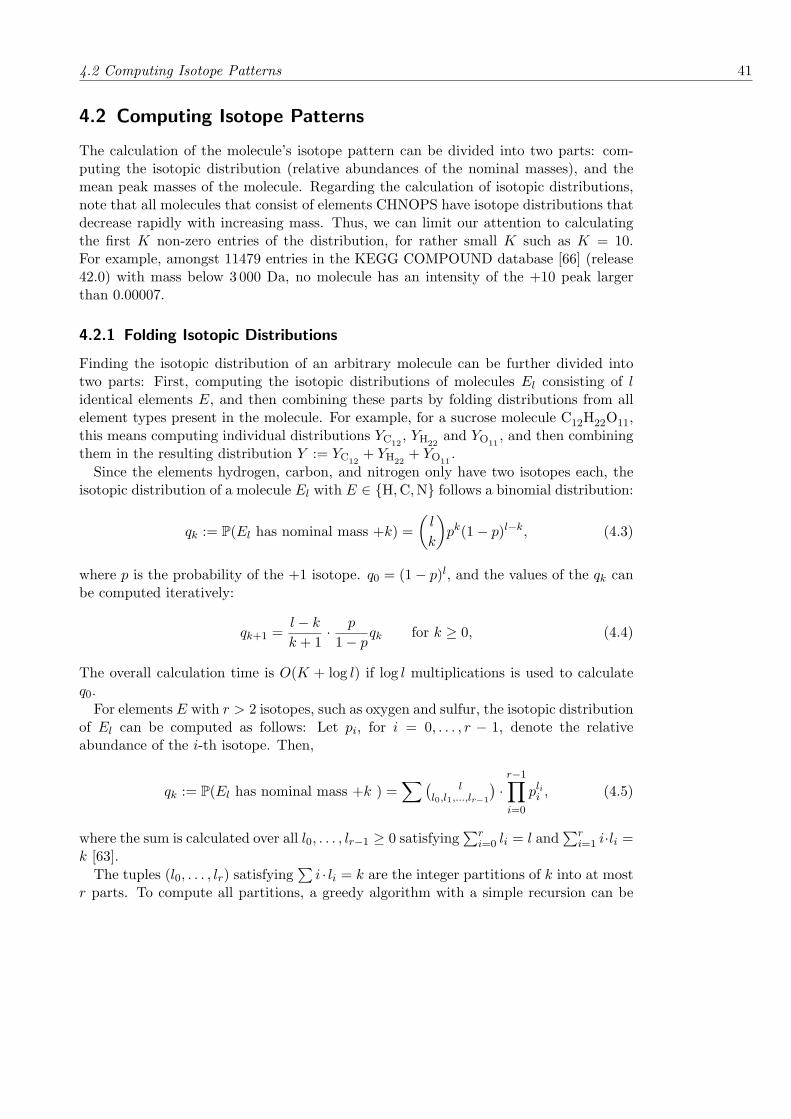
4.2 Computing Isotope Patterns 41
4.2 Computing Isotope Patterns
The calculation of the molecule’s isotope pattern can be divided into two parts: com-puting the isotopic distribution (relative abundances of the nominal masses), and themean peak masses of the molecule. Regarding the calculation of isotopic distributions,note that all molecules that consist of elements CHNOPS have isotope distributions thatdecrease rapidly with increasing mass. Thus, we can limit our attention to calculatingthe first K non-zero entries of the distribution, for rather small K such as K = 10.For example, amongst 11479 entries in the KEGG COMPOUND database [66] (release42.0) with mass below 3 000 Da, no molecule has an intensity of the +10 peak largerthan 0.00007.
4.2.1 Folding Isotopic Distributions
Finding the isotopic distribution of an arbitrary molecule can be further divided intotwo parts: First, computing the isotopic distributions of molecules El consisting of lidentical elements E, and then combining these parts by folding distributions from allelement types present in the molecule. For example, for a sucrose molecule C12H22O11,this means computing individual distributions YC12
, YH22and YO11
, and then combiningthem in the resulting distribution Y := YC12
+ YH22+ YO11
.Since the elements hydrogen, carbon, and nitrogen only have two isotopes each, the
isotopic distribution of a molecule El with E ∈ H,C,N follows a binomial distribution:
qk := P(El has nominal mass +k) =(
l
k
)pk(1− p)l−k, (4.3)
where p is the probability of the +1 isotope. q0 = (1− p)l, and the values of the qk canbe computed iteratively:
qk+1 =l − k
k + 1· p
1− pqk for k ≥ 0, (4.4)
The overall calculation time is O(K + log l) if log l multiplications is used to calculateq0.
For elements E with r > 2 isotopes, such as oxygen and sulfur, the isotopic distributionof El can be computed as follows: Let pi, for i = 0, . . . , r − 1, denote the relativeabundance of the i-th isotope. Then,
qk := P(El has nominal mass +k ) =∑ (
ll0,l1,...,lr−1
)·
r−1∏i=0
plii , (4.5)
where the sum is calculated over all l0, . . . , lr−1 ≥ 0 satisfying∑r
i=0 li = l and∑r
i=1 i·li =k [63].
The tuples (l0, . . . , lr) satisfying∑
i · li = k are the integer partitions of k into at mostr parts. To compute all partitions, a greedy algorithm with a simple recursion can be

42 4. Molecular Formula Identification of Metabolites
employed. However, this approach faces the problem that the number of summands in(4.5) grows rapidly, at least as a polynomial in k of degree r − 1 [123].
Alternatively, the isotopic distributions of oxygen Ol and sulfur Sl can be computedby consecutive folding of the corresponding distributions using a Russian multiplicationscheme discussed below.
Given two discrete random variables Y and Y ′ with state spaces Ω,Ω′ ⊆ N, we cancompute the combined distribution of the random variable Z := Y + Y ′ by folding thedistributions as follows:
P(Z = n) =∑
kP(Y = k) · P(Y ′ = n− k). (4.6)
Computing the first K values of this sum requires O(K2) time. To fold isotopic distri-butions of individual elements, Kubinyi proposed [75] to use a Russian multiplicationscheme: We start with the molecule consisting of a single element E, and using for-mula (4.6) compute the isotopic distributions of molecules with 2, 4, 8, . . . atoms. Forexample,
Z1 + Z2 + Z3 + Z4 + Z5 + Z6 + Z7 =((Z1 + Z2) + (Z3 + Z4)
)+ (Z5 + Z6) + Z7,
where Zi denote independent and identically-distributed (i. i. d.) random variables.Then, we combine these distributions to compute that of El. This adds a logarithmicfactor to the algorithm’s total running time, altogether O(K2 log l).
In applications, the distributions of elements with more than two isotopes can becomputed not on the fly but during preprocessing. For all l ≤ L, a lookup table is createdthat uses O(KL) space for every such element, where L is small: In our applications, themass range of the analyzed biomolecules usually does not exceed 2 000 Da; 128 oxygenatoms already have a mass of about 2 048 Da, being larger than the relevant upperbound.
After the isotopic distributions of individual elements have been computed (C, H, N)or looked up from memory (O, S), we combine them by folding using formula (4.6).Doing so requires O(|Σ| ·K2) time in total.
Note that we can use Fourier transforms of isotopic distributions, and instead of foldingthe distributions, multiply the Fourier transforms [100]. This can eventually substitutethe K2 factor in the algorithm’s running time by the K log K factor. However, as werestrict ourselves to rather small K such as K = 10, this will not speed up the algorithmin practice. Moreover, this approach may face the problem of numerical errors.
4.2.2 Folding Peak Masses
We now move to the more intriguing issue of efficiently calculating the mean peak massesof a distribution. Computing the mean peak mass using formula (4.2) is highly inefficient,because we have to calculate the sum over all isotope species. Pruning techniques havebeen proposed to speed up computation [131], but they result in a drop of accuracy [101].We now present a simple approach to compute the mean masses similar to the foldingof isotopic distributions:

4.2 Computing Isotope Patterns 43
Given two molecules with monoisotopic nominal masses N and N ′, and isotopic dis-tributions Y = Y1 + · · ·+Yl and Y ′ = Y ′
1 + · · ·+Y ′L, respectively. Let mk and m′
k be themean peak masses of the +k peaks, and pk := P(Y = N + k) and qk := P(Y ′ = N ′ + k)denote the respective probabilities. Consider the random variable Z = Y + Y ′ withmonoisotopic nominal mass N = N + N ′.
Theorem 1. The mean peak mass mk of the +k peak of the random variable Z = Y +Y ′
can be computed as:
mk =1∑k
j=0 pjqk−j
·k∑
j=0
pjqk−j
(mj + m′
k−j
)(4.7)
Note that∑k
j=0 pjqk−j = P(Z = N + k).
Proof. Let ~N = (N1, . . . , Nl) ∈ Nl and ~N ′ = (N ′1, . . . , N
′L) ∈ NL be vectors of nominal
masses. We denote∑ ~N :=
∑li=1 Ni and
∑ ~N ′ :=∑L
i=1 N ′i . Let ~Y := (Y1, . . . , Yl) and
~Y ′ := (Y ′1 , . . . , Y
′L) be vectors of the input random variables, and note that
P(~Y = ~N, ~Y ′ = ~N ′) = P(~Y = ~N) · P( ~Y ′ = ~N ′)
due to the independence of the underlying random variables. Finally, we set µ( ~N) =∑li=1 µ(Ni) and define µ( ~N ′) analogously.
Ignoring the normalization factor, we can rearrange formula (4.2) as
P(Z = N + k) · mk =∑
P ~N+P ~N ′=N+k
P(~Y = ~N, ~Y ′ = ~N ′) ·(µ( ~N) + µ( ~N ′)
).
Now observe that this formula can be divided into two independent sums of the form
∑P ~N+
P ~N ′=N+k
P(~Y = ~N, ~Y ′ = ~N ′) · µ( ~N) (4.8)
and a second summand, where µ( ~N) is substituted with µ( ~N ′).

44 4. Molecular Formula Identification of Metabolites
We now concentrate on (4.8):∑P ~N+
P ~N ′=N+k
P(~Y = ~N, ~Y ′ = ~N ′) · µ( ~N)
=k∑
j=0
∑P ~N=N+j
∑P ~N ′=N ′+k−j
P(~Y = ~N)P( ~Y ′ = ~N ′) · µ( ~N)
=k∑
j=0
∑P ~N=N+j
P(~Y = ~N) · µ( ~N)∑
P ~N ′=N ′+k−j
P( ~Y ′ = ~N ′)
=k∑
j=0
∑P ~N=N+j
P(~Y = ~N) · µ( ~N) · P(Y ′1 + · · ·+ Y ′
L = N ′ + k − j)
=k∑
j=0
P(Y ′ = N ′ + k − j)∑
P ~N=N+j
P(~Y = ~N) · µ( ~N)
=k∑
j=0
qk−jpjmj ,
where the last equality follows from the definition of mj ,
mj =1pj
∑P ~N=N+j
P(~Y = ~N) · µ( ~N).
Analogously, we can show that
∑P ~N+
P ~N ′=N+k
P(~Y = ~N, ~Y ′ = ~N ′) · µ( ~N ′) =k∑
j=0
qk−jpjm′j ,
which concludes the proof of the theorem.
The theorem allows us to “fold” mean peak masses of two distributions to computethe mean peak masses of their sum. This means that we can compute the mean massesas efficiently as the distribution itself, i.e., in O(K2 log l) time. This improves on thebest present-day approach [101], substituting the linear running time dependence on thenumber of atoms l by its logarithm.
4.3 Scoring Candidate Molecules
Our task is to distinguish between candidate molecules produced by the decompositionof the monoisotopic mass, and to choose the candidate, whose isotope pattern matchesthe measured peak list best. In Section 4.1, we have seen how to efficiently calculate the

4.3 Scoring Candidate Molecules 45
isotope pattern from the molecular formula. Now we want to compare this simulatedisotope pattern with the measured peak list by matching the pairs of peaks in both.
To assess the similarity between mass spectra, Zhang and Chait [134] and Zhang et al. [133]propose the probabilistic approach employing Bayesian Statistics:
P(Mj |D,B) =P(Mj |B) P(D|Mj ,B)∑i P(Mi|B) P(D|Mi,B)
,
where Mi are the models (the candidate molecules), D is the data (the measured peaklist), and B stands for any prior background information.
Concerning the background information, we first employ the prior knowledge about thecandidate molecules, by assigning the prior probability P(Mj |B) zero for all moleculesbut the decompositions of the monoisotopic mass. Next, we model the chemical bondingrules by setting the prior probability to zero for molecular formulas that do not satisfy theconditions of the Senior’s theorem (see Section 2.1 on page 5). For example, moleculesviolating Senior’s third rule are rare, particularly for natural compounds: less than0.16 % of substances in the KEGG COMPOUND database violate this rule.
Other priors such as the hetero-to-carbon ratio [73] exist that are typically derivedempirically based on the already known compounds. To keep the comparison unbiasedfor unknown molecules, we deliberately avoid further use of such priors.
Next, we assign probabilities to the measured peak masses and intensities. LetP(Mj |mj) denote the probability to detect peak j at mass Mj when its actual massis mj , and P(fj |pj) denote the probability to detect peak j with intensity fj when itsactual intensity is pj . Then, assuming independence, particularly from background in-formation, the probability to observe the measured peak list, given a certain candidatemolecule and background information can be calculated as follows:
P(D|M,B) =∏j
P(Mj |mj)∏j
P(fj |pj) (4.9)
Note that the peak intensities are, in fact, not independent, since they sum up to one,but the product (4.9) can be viewed as a rough estimate of the true probability.
4.3.1 Estimating Probabilities of Peak Masses
As mentioned in Section 2.5.3, experimentalists typically assume that the mass deviationof a mass spectrometer follows the Gaussian distribution with mean zero. Given therelative mass accuracy α of the measurement (in ppm), we can assign the standarddeviation σj := 1
3α 10−6 Mj for peak j, assuming that more than 99.7 % of measurementsbelong to the mass range [−3σj ,+3σj ]. However, we notice that peaks of high intensityreveal better mass accuracy than those of low intensity, which can be referred to thecomplications of extracting the low intensity peaks from the background noise. Our datashows an approximately linear correlation between peak intensity and mass accuracy.To take this into account, we use two mass accuracies α1 (at full intensity) and α0 (atminimal intensity), and calculate the standard deviation for peak j as follows:
σj := 13
(pj α1 + (1− pj)α0
)· 10−6 Mj . (4.10)

46 4. Molecular Formula Identification of Metabolites
Additionally, imperfections in calibrating mass spectrometers lead to a systematic massshift between different peak masses of the same spectrum. This occurs frequently evenfor high resolution MS. To eliminate this error for all masses except the monoisotopicmass, we do not compute the mass differences of the +1,+2, . . . peaks directly butinstead, the difference to the monoisotopic mass, Mj −M0 against mj −m0, for j ≥ 1.
Given a peak with theoretical mass mj , we want to estimate the probability to ob-serve a peak at mass Mj in the measured peak list, or, saying strictly, we calculate theprobability of detecting a mass difference of |Mj −mj | or larger. This probability canbe computed using the complementary error function “erfc”:
P(Mj |mj) = P(mass difference ≥ xj) = erfc( |xj |√
2 σj
)=
2√2π
∫ ∞
ze−t2/2dt (4.11)
with z := |xj |σj
, where x0 = (M0−m0)/m0 and xj = (Mj−M0−mj +m0)/mj , for j ≥ 1,denote the relative mass differences.
4.3.2 Estimating Probabilities of Peak Intensities
Concerning the peak intensities, a systematic shift in the measured data can be observed:The peaks of high intensity are overestimated, while the peaks with low intensity areunderestimated in the measured peak list, see Figures 4.1 and 4.2.
This problem can be attributed to inaccuracies of peak intensity calculation on thepreprocessing step: peak picking algorithms typically determine peak intensities using asignal-to-noise ratio or height above a certain baseline (see Section 2.5.2 on page 22). Thecalculation of the baseline, in turn, is done using some empirical estimates that can beimprecise. These inaccuracies have unequal impact on peaks of different intensities. Toadjust this systematic bias, we introduce a user-defined parameter off . This parameteris added to the measured intensities, which are then re-normalized again. In the nextsection, when evaluating our algorithm, we provide more details on setting the parameteroff .
After applying the correction to the measured data, we observe that log ratios betweenmeasured and theoretical peak intensity log(fj/pj) are roughly normally distributed.Similar to mass differences, we introduce two precision parameters β1 (at full intensity)and β0 (at minimal intensity) to be set (in percent), and compute the standard deviationfor peak j as follows:
σj := 13 log
(1 + pj
β1
100 + (1− pj) β0
100
),
so that more than 99.7 % of ratios log(fj/pj) belong to the range [−3σj ,+3σj ]. Now,the computation of probability P(fj |pj) can be done analogously to (4.11).
4.4 Experimental Results
Datasets. To evaluate our method, two datasets measured on two instruments wereused. Mass spectra with single charge were measured from several organic (macro)mole-cules, composed of elements CHNOPS. For every such spectrum, the molecular formula

4.4 Experimental Results 47
-0.08
-0.06
-0.04
-0.02
0
0.02
0.04
0.06
0.08
0 0.1 0.2 0.3 0.4 0.5 0.6 0.7 0.8 0.9
inte
nsity
diff
eren
ce
measured intensity
off = 0off = +0.02
Figure 4.1: Differences between measured and theoretical peak intensities and mass accu-racies for the FT-ICR dataset in comparison: measured intensities computedwithout correction (crosses), measured intensities computed with correctionoff = +0.02 (circles). The difference is computed as measured peak intensityminus theoretical peak intensity.
of the sample molecule is known. The spectra were acquired over a period of two years;the molecules range in mass from 117 to about 1 000 Da. Peak detection and estimationof the peak masses and intensities were performed using vendor software.
The first dataset consists of 153 peak lists. Electrospray ionization (ESI) experimentswere conducted using the Fourier Transform Ion Cyclotron Resonance (FT-ICR) massspectrometer APEX III (Bruker Daltonik GmbH, Bremen, Germany). The FT-ICR MSwas equipped with a 7.0 T, 160 mm bore superconducting magnet, infinity cell, andinterfaced to an external (nano)ESI ion source. Measured data was externally masscalibrated. The five analysis parameters were chosen as α1 = 3, α0 = 6, β1 = 10,β0 = 90, and off = +0.02.
The second dataset consists of 86 peak lists. ESI experiments were conducted using theoa-TOF mass spectrometer MicrOTOF (Bruker Daltonik GmbH, Bremen, Germany).Quasi-internal mass calibration was used, by measurement of an infused calibrant priorto the compound of interest. For the oa-TOF analysis, the parameters were set to α1 = 5,α0 = 6.5, β1 = 10, β0 = 90, and off = +0.02.
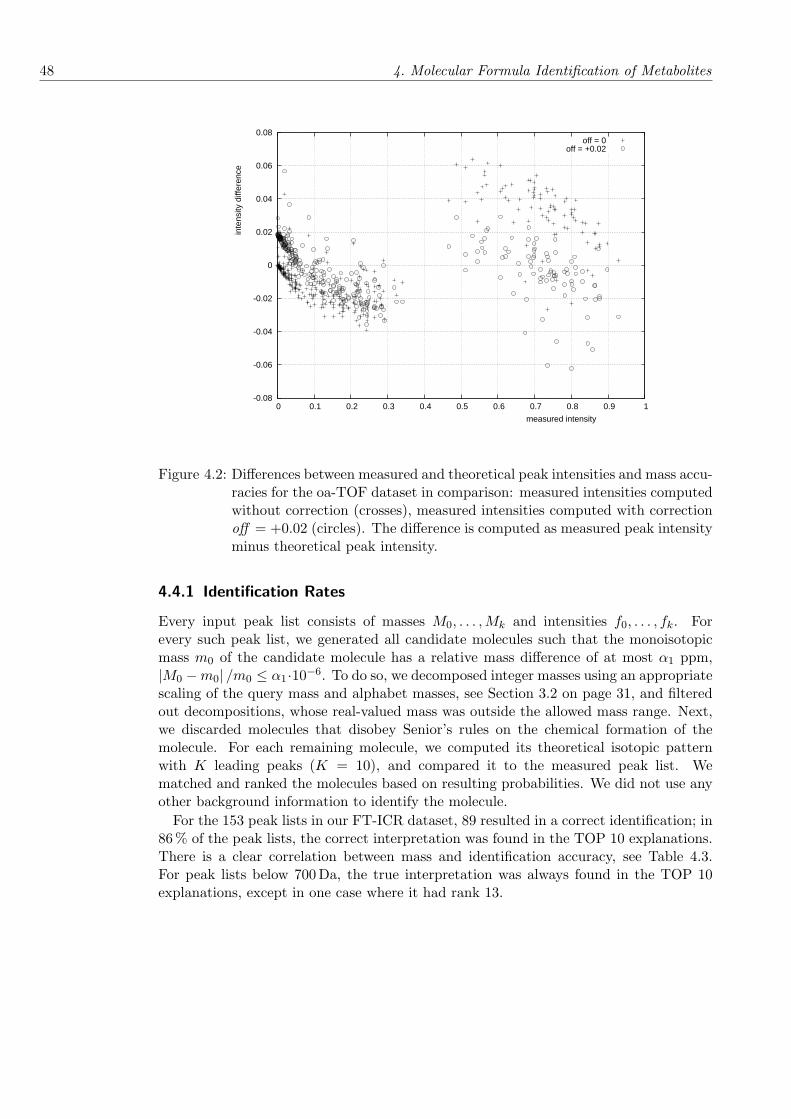
48 4. Molecular Formula Identification of Metabolites
-0.08
-0.06
-0.04
-0.02
0
0.02
0.04
0.06
0.08
0 0.1 0.2 0.3 0.4 0.5 0.6 0.7 0.8 0.9 1
inte
nsity
diff
eren
ce
measured intensity
off = 0off = +0.02
Figure 4.2: Differences between measured and theoretical peak intensities and mass accu-racies for the oa-TOF dataset in comparison: measured intensities computedwithout correction (crosses), measured intensities computed with correctionoff = +0.02 (circles). The difference is computed as measured peak intensityminus theoretical peak intensity.
4.4.1 Identification Rates
Every input peak list consists of masses M0, . . . ,Mk and intensities f0, . . . , fk. Forevery such peak list, we generated all candidate molecules such that the monoisotopicmass m0 of the candidate molecule has a relative mass difference of at most α1 ppm,|M0 −m0| /m0 ≤ α1·10−6. To do so, we decomposed integer masses using an appropriatescaling of the query mass and alphabet masses, see Section 3.2 on page 31, and filteredout decompositions, whose real-valued mass was outside the allowed mass range. Next,we discarded molecules that disobey Senior’s rules on the chemical formation of themolecule. For each remaining molecule, we computed its theoretical isotopic patternwith K leading peaks (K = 10), and compared it to the measured peak list. Wematched and ranked the molecules based on resulting probabilities. We did not use anyother background information to identify the molecule.
For the 153 peak lists in our FT-ICR dataset, 89 resulted in a correct identification; in86 % of the peak lists, the correct interpretation was found in the TOP 10 explanations.There is a clear correlation between mass and identification accuracy, see Table 4.3.For peak lists below 700 Da, the true interpretation was always found in the TOP 10explanations, except in one case where it had rank 13.

4.4 Experimental Results 49
For 86 peak lists in the oa-TOF dataset the correct molecular formula was found inthe TOP 10 interpretations in all but two cases. Moreover, 79 out of 86 compounds wereidentified correctly, which corresponds to an identification rate of over 90 %, see Table 4.3.Better identification results on the oa-TOF dataset with lower mass accuracy show thecrucial importance of including intensity measurements into the candidate evaluation.We note that the intensity accuracy of the oa-TOF instrument is significantly higherthan that of the FT-ICR.
mass no. rank in output list no. molecular formulasrange pl. 1 2 3–5 6–10 11+ int. real chem. time
200–300 13 11 2 0 0 0 67 37.2 8.6 1.5300–400 37 28 5 2 2 0 200 109 10.4 4.3400–500 57 39 6 6 5 1 579.5 318.2 22.8 13.5500–600 7 5 2 0 0 0 1800.4 990.3 59.6 40.1600–700 4 3 0 0 1 0 2668.5 1454 37.3 55700–800 5 0 1 1 1 2 8797.8 4812 247 232800–900 14 3 2 1 3 5 14781.6 8101 534.6 485
900–1000 16 0 1 1 1 13 31805.7 17448 1570 1281
mass no. rank no. molecular formulasrange pl. 1 2–6 11+ int. real chem. time
100–200 7 7 0 0 11.3 7.4 1.9 0200–300 21 21 0 0 60.1 40.1 4.6 1.4300–400 27 26 1 0 297.8 199.7 22.6 8.1400–500 15 14 1 0 725.6 484.1 32.4 17.3500–600 10 7 2 1 1479.1 988.9 54.3 36600–700 1 1 0 0 4600 3080 276 130700–800 2 1 1 0 10336 6909 578 461800–900 3 2 0 1 18172.3 12146 914.3 757
Table 4.3: Number of correct molecular formulas at specific positions of the output list,for the FT-ICR dataset (top) and the oa-TOF dataset (bottom). We reportthe number of peak lists in this mass range (no. pl.), as well as the aver-age number of molecular formulas over all molecules in the mass range (no.molecular formulas). We distinguish between the number of integer decom-positions (int.), the number of decompositions over real-valued masses (real),and the number of those molecular formulas that satisfy chemical bondingrules (chem.). Finally, we give the average running time in milliseconds perpeak list (time).
Regarding the scoring parameter off , for both of our datasets we used the same valueoff = +0.02. We have also tested the robustness of our method by varying different

50 4. Molecular Formula Identification of Metabolites
scoring parameters: Identification accuracy remained relatively stable for small distur-bances of parameter values, confer Table 4.4 and Figures 4.3 and 4.4. In applications,parameters can be estimated using a small training set.
β1 β0 identification raterank1 ( %) top10 (%)
5 70 58.82 86.9315 70 58.82 86.935 80 58.82 85.62
10 70 58.17 86.9310 90 58.17 86.2715 90 58.17 86.2720 70 58.17 85.625 90 57.52 86.275 100 57.52 86.27
10 100 57.52 86.2715 80 57.52 86.2720 80 57.52 86.2720 90 57.52 86.275 110 57.52 85.62
10 80 57.52 85.6220 110 57.52 85.6210 110 56.86 85.6215 100 56.86 85.6215 110 56.86 85.6220 100 56.86 85.62
β1 β0 identification raterank1 ( %) top10 (%)
5 90 91.86 97.675 100 91.86 97.67
10 90 91.86 97.6710 100 91.86 97.6715 90 91.86 97.6715 100 91.86 97.6720 90 91.86 97.6720 100 91.86 97.675 80 90.70 97.675 110 90.70 97.67
10 80 90.70 97.6710 110 90.70 97.6715 80 90.70 97.6715 110 90.70 97.6720 80 90.70 97.6720 110 90.70 97.675 70 89.53 97.67
10 70 89.53 97.6715 70 89.53 97.6720 70 89.53 97.67
Table 4.4: Identification rates for various intensity precisions β1 (at full intensity) and β0
(at minimal intensity), for the FT-ICR dataset (left) and the oa-TOF dataset(right). We set mass accuracies α1 (at full intensity) and α0 (at minimalintensity) to fixed values: α1 = 3, α0 = 6 for the FT-ICR dataset, andα1 = 5, α0 = 6.5 for the oa-TOF dataset. Parameter off is set to +0.02. Onecan see that our method is very robust to small variations of the parameters.
Running Times. All algorithms were implemented in Java, and executed within theSIRIUS software environment, see Chapter 7. All 239 peak lists were analyzed on aPentium M 1.5 GHz processor with blowup b = 5 · 104, using only a few Megabyteof memory. This results in running times of less than 1.3 seconds per peak list for thecomplete analysis of one peak list. Clearly, running times depend on masses of molecules,again see Table 4.3. Increasing the blowup beyond 5 · 104 increased the running times,presumably because the smaller table can be kept in the processor cache.

4.4 Experimental Results 51
40
45
50
55
60
65
70
75
80
85
90
0 0.005 0.01 0.015 0.02 0.025 0.03 0.035 0.04 0.045 0.05 0.055
iden
tific
atio
n ac
cura
cy, %
off
rank1top10
Figure 4.3: Identification rates for various parameters off , for the FT-ICR dataset incomparison: Percentage of correct identifications (crosses), percentage oftrue molecular formulas found in TOP 10 explanations (circles). We setmass and intensity precisions to fixed values: α1 = 3, α0 = 6, β1 = 10,β0 = 90.
40
50
60
70
80
90
100
0 0.005 0.01 0.015 0.02 0.025 0.03 0.035 0.04 0.045 0.05 0.055
iden
tific
atio
n ac
cura
cy, %
off
rank1top10
Figure 4.4: Identification rates for various parameters off , for the oa-TOF dataset incomparison: Percentage of correct identifications (crosses), percentage oftrue molecular formulas found in TOP 10 explanations (circles). We setmass and intensity precisions to fixed values: α1 = 5, α0 = 6.5, β1 = 10,β0 = 90.


5 Deriving Peptide Compositions
In the previous section, we have seen that using only a high quality isotope pattern of asample molecule, it is possible to identify the molecular formula of unknown metabolite.For proteins, one however encounters the problem that the same molecular formula maycorrespond to multiple peptides even when abstracting from the order of amino acids inthe peptide sequence. In this chapter, we present a novel approach to efficiently derivethe amino acid composition of an unknown peptide from its molecular formula.
Novel mass spectrometry techniques allow us to determine the mass of a samplemolecule with very high accuracy of 5 ppm, and sometimes below 1 ppm [89,58]. Thesetechniques are increasingly coupled with high-throughput separation techniques such as(ultra) high performance liquid chromatography (HPLC), and have become one preferredmethod for the analysis of peptides [55, 112]. This setup becomes of high importancein particular when tackling non-trivial issues in proteomics, such as detecting the post-translational modifications [118], or non-ribosomal peptides that are not directly encodedin the genome [6]. With the advent of new MS instruments (Bruker MicrOTOF, ThermoElectron LTQ Orbitrap, Waters SYNAPT-MS), mass spectra with very high mass accu-racy will be routinely acquired for protein identification and quantification in the nearfuture [81].
Given an isotope pattern of an unknown peptide, in theory, one could use an algorith-mic procedure similar to the one described above for the identification of metabolites:one can decompose the monoisotopic mass of the peptide to obtain amino acids candi-date sequences, and then compare and score candidates using their simulated isotopepatterns. However, this approach is infeasible in practice due to the several reasons:First, masses of peptides have to be decomposed over an alphabet of 19 standard aminoacids, compared to 6 elements in CHNOPS, which is used for the majority of metabolites.Thus, the number of possible amino acid decompositions is significantly larger than ofCHNOPS decompositions, see Section 3.2.1 on page 33: There exist about 3.96 · 1011
amino acid decompositions with mass up to 2 500 Dalton, see Figure 3.3. Moreover, sev-eral peptides can have identical molecular formula even when ignoring the order of aminoacids: Besides leucine (L) and isoleucine (I), another example are peptides consisting oftwo glycine (G) versus a single asparagine (N), both with molecular formula C4H8N2O3
(see Table 2.2 on page 10). Using the above scoring procedure, we cannot distinguishbetween amino acids compositions with the same molecular formula, and thus, the sameisotope pattern. In addition, the sample may be contaminated by metabolite moleculesthat have a molecular formula which cannot be explained by any peptide. So, insteadof determining peptide compositions from the isotope pattern directly, it is much morereasonable first to find out the molecular formula of a sample from its isotope pattern,and then to calculate all amino acid compositions that correspond to this molecular
53

54 5. Deriving Peptide Compositions
formula. Using the molecular formula of a sample molecule, we can also easily filter outany contaminant, whose molecular formula cannot correspond to any peptide.
Our input is the molecular formula of an unknown peptide. We want find all aminoacid compositions that match the given molecular formula. We formulate the problemas a joint decomposition of a set of queries on the number of carbon, hydrogen, andother elements that amino acid residues consist of.
The remainder of this chapter is organized as follows: First, we give a formal definitionof a problem and outline its possible solutions. Then, we present our approach based onthe dimension reduction technique that transforms an instance of the multi-dimensionaldecomposition problem to the one-dimensional decomposition problem, which in turncan be efficiently solved using methods presented in Chapter 3. Finally, we provide anexperimental evaluation of the algorithm’s running time, both on simulated data andpeptides from experimental mass spectra. We find that our mixed matrix approach isthe fastest method for generating solutions, and is about two orders of magnitude fasterthan the next best algorithm.
5.1 Peptide Molecular Formula Decomposition Problem
Recall that proteins and peptides are built from five elements hydrogen (symbol H),carbon (C), nitrogen (N), oxygen (O), and sulfur (S). For each amino acid its exactmolecular formula is known, see Table 2.2.
Formally, the Peptide Molecular Formula Decomposition Problem (PMFDP) can bestated as follows:
Given a molecular formula b = (b1, . . . , bd) and a matrix Ad×n = (ai,j) con-taining the abundances of all elements in amino acid residues, with bi ∈ N0
and ai,j ∈ N+, for i = 1, . . . , d and j = 1, . . . , n, where d is the numberof amino acid residues and n is the number of elements that amino acidresidues consist of, find all decompositions x = (x1, . . . , xn) with xj ∈ N0,for j = 1, . . . , n, such that Ax = b.
If we have d = n many equations, then A is a square matrix, and if its rows arelinearly independent, we can compute its inverse A−1. We then only need to checkwhether x = A−1b has only non-negative integer entries, what can be done in constanttime. In the remainder of this chapter, we assume d n.
Considering n = 19 number of amino acid residues that made up from d = 5 elementsCHNOS, we thus search for 19-dimensional vector x using the input molecular formula bover the elements CHNOS. Note that only amino acids methionine (M) and cysteine (C)contain sulfur. Thus, we can use a simple technique to further simplify the problem if ourinput molecular formula contains k sulfur elements: we first distribute these elementsbetween methionine and cysteine, iterating over all k combinations M0Ck, M1Ck−1, . . . ,MkC0. In each case, we reduce the input molecular formula respectively, and computethe decomposions of the resulting formulas over the remaining 17 amino acids A, D, E,

5.1 Peptide Molecular Formula Decomposition Problem 55
F, G, H, K, L, N, P, Q, R, S, T, V, W, Y:
A :=
3 4 5 9 2 6 6 6 4 5 5 6 3 4 5 11 95 5 7 9 3 7 12 11 6 7 8 12 5 7 9 10 91 1 1 1 1 3 2 1 2 1 2 4 1 1 1 2 11 3 3 1 1 1 1 1 2 1 2 1 2 2 1 1 2
,
b =
# carbon
# hydrogen# nitrogen# oxygen
, Ax = b (5.1)
Here, x is a 17-dimensional vector representing the remaining amino acid residues.Finally, after solutions of (5.1) are obtained, for each of the reduced formulas, we
extend each solution vector x by adding the corresponding number of methionine andcysteine, and combine them in our final set of decompositions.
5.1.1 Related Problems and Solutions
Our problem is a special case of a system of linear Diophantine equations. Unlike inPMFDP, the coefficients of matrix A in the linear Diophantine systems can be nega-tive integers. This seemingly negligable relaxation makes a significant impact on thedifferences in the number of solutions of these two problems: while PMFDP is limitedto a finite number of possible explanations, a system of linear Diophantine equationsgenerally has an infinite number of solutions.
To see this, consider an instance of one-dimensional Equality Constrained IntegerKnapsack Problem
a1x1 + a2x2 + · · ·+ anxn = b (5.2)
where aj are integer-valued coefficients satisfying aj ≥ 0, b ≥ 0. We search for all solutionvectors x = (x1, . . . , xn) such that all xj are non-negative integers. Note that if thereexist indices i, j with ai > 0 and aj < 0, as allowed in a linear Diophantine equation,and if (5.2) has at least one solution, then there is an infinite number of solutions.
Our problem can be also seen as d one-dimensional knapsack equations (5.2) thatwe want to solve simultaneously, and is equivalent to a multi-dimensional EqualityConstrained Integer Knapsack Problem. Unlike in a typical formulation of a multi-dimensional Integer Knapsack Problem [70], we are not looking for the maximization ofa set of objective functions, but instead for the exact matches of these functions to theset of given queries.
As for a special case of a more general problem, approaches, that exist for solving asystem of linear Diophantine equations, can be also employed to solve PMFDP. Mostof them have in common to increase the solution vector until an exact hit or a failureis achieved. We call this the branch-and-bound algorithm. In the remainder of thissection, we describe this and other existing methods to solve PMFDP in some detail,and afterwards present our novel mixed matrix approach to efficiently derive the peptidecomposition from its molecular formula.

56 5. Deriving Peptide Compositions
Branch-And-Bound Algorithm One simple method to solve our problem is a branch-and-bound search, which general idea is to add amino acids as long as for each element,the resulting molecule contains at most as many atoms as the input molecule, and toreport exact hits.
The algorithm starts by examining all possibilities for the first amino acid alanine andbranches, then repeats the same for aspartic acid, and so on until it reaches the lastamino acid tyrosine. Then, the algorithm checks whether the number of elements inthe current peptide decomposition is equal to the number of elements in the molecularformula, and output exact hits. The algorithm branches using the recursive calls andon each recursion step it maintains a current decomposition c, an index i of an aminoacid, and the current bounds on the number of carbon, hydrogen, nitrogen and oxygenin the vector b. In Figure 5.1, we provide the pseudo-code of the algorithm. As an
Algorithm branch-and-bound (decomposition c, index i, bounds b)1 if bj = 0 for all j = 1, . . . , d then2 output c;3 return;4 end if;5 ni ← 0;6 while bj >= 0 for all j = 1, . . . , d do7 if i > 1 then8 ci ← ni;9 branch-and-bound(c, i− 1, b);10 else11 c1 ← b1/A1,1;12 if bj = Aj,1 ∗ c1 for all j = 1, . . . , d then13 output c;14 return;15 end if;16 end if;17 bj ← bj −Aj,i for all j = 1, . . . , d;18 end while;19 done.
Figure 5.1: branch-and-bound algorithm for finding all peptide compositions using themolecular formula. For a molecular formula b = (b1, . . . , bd), where d = 4 isthe number of bounds, branch-and-bound(0, k, b) will recursively produceall peptide compositions over matrix Ad×k that satisfy b.
alternative to the branch-and-bound search, we can compute the molecular formulasof all amino acid compositions up to a fixed mass during preprocessing, and employhashing to efficiently find those decompositions matching the input molecular formula.Unfortunately, due to the large number of possible solutions, in practice this approachsuffers from large requirements of memory: Recall that there exist about 3.96 · 1011

5.1 Peptide Molecular Formula Decomposition Problem 57
amino acid decompositions with mass up to 2500 Da.
Decomposition Algorithms In Chapter 3, we have seen how to efficiently solve aninstance of one-dimensional knapsack problem (5.2). Now, as we move to a multi-dimensional problem, a simple algorithm to compute all solutions of Ax = b, is tochoose one row i ≤ d as the master row, then to find all solutions of the one-dimensionalknapsack ai,1x1 + · · · + ai,nxn = bi and, finally, for each solution of the master row tocheck if it also satisfies the other equations of our multi-dimensional knapsack. We callthis the naıve decomposition algorithm. Solutions of the master row can be found bybacktracing through the Extended Residue (ER) table, as described in Section 3.1.2.However, this involves generating many decompositions unnecessarily.
Instead of discarding the false positives after the completion of the recursive algorithmover the master row, we can introduce several ER tables that correspond to other rowsof Ax = b, and perform the backtracing over multiple instances simultaneously: Themultiple decomposition algorithm also picks up a master equation to decompose, buttests during recursion if all other equations of Ax = b besides the master equation canstill be satisfied using the current partial solution. If this is no longer possible, thenthe algorithm stops and discards the current partial solution. Doing so, this approachdoesn’t generate any false positives, but it requires additional memory to store the datafor several decomposition instances.
5.1.2 Multi-dimensional Integer Knapsack
As we have seen in Equation (3.3), the number of mass decompositions over the alphabetof size n increases with a polynomial of degree n − 1. It is thus logical to reduce n asmuch as possible, if we can do so. Actually, the multi-dimensional knapsack allows us tolower n: To this end, we apply a Gaussian elimination to the matrix A to find a lowertriangular matrix L ∈ Rd×d and an upper triangular matrix R = (ri,j) ∈ Rd×n such thatA = LR. Then, Ax = b if and only if Rx = L−1b =: b′, where L−1 is known. Everysolution of the original equation must henceforth satisfy the bottom equation of R,
0 · x1 + · · ·+ 0 · xd−1 + rd,dxd + · · ·+ rd,nxn = b′d (5.3)
that has at most n − d + 1 non-zero coefficients. Now, our idea is to search for alldecompositions of the bottom equation, and for each solution, to test if it is also asolution of Ax = b.
Since all coefficients of the matrix A are integers, we can easily assure that afterapplying Gaussian elimination, the same holds for the coefficients of the output matrixR. On the other hand, we cannot guarantee that ri,j ≥ 0 holds for all coefficients afterGaussian elimination, even if all entries in the matrix A are non-negative. In particular,there may be negative coefficients in the bottom row of R. But as mentioned above,this means that the bottom equation has an infinite number of solutions, provided thatthere exists at least one solution. Therefore, we have to avoid that the bottom row ofR contains negative coefficients. To find Gaussian eliminations arrangements where this

58 5. Deriving Peptide Compositions
condition holds, we may swap the columns and rows of A: We select a permutation π ofthe rows of A, and a permutation σ of the columns of A that brings d columns to thefront but ignores the remaining n− d columns. We have d! possibilities to select π, and(n− d + 1) · · ·n possibilities to select d front rows of A in σ.
We apply the following simple invariant of the Gaussian elimination method in ourcomputations, see the pseudo-code of the algorithm on page 68: Assume that rowsand columns of matrix A have been already swapped. For the sake of simplicity, wewill compute L−1, instead of L. We initialize L−1 = (li,j) ← I as the identity matrixand R← A. We use the row i of matrix R as our master row, and repeat the followingprocedure for i = 1, . . . , d−1 (lines 3-19): We take the element ri,i in the master row, andthe element ri′,i below the main diagonal for each row i′ = i+1, . . . , d, as our multipliersmi and mi′ (lines 9-10), and iterate through columns j = i, . . . , n, and modify elementsin the row i′ as following: ri′,j = mi′ri,j −miri′,j . Then, ri′,i = 0 must hold. Similarly,for columns j′ = 1, . . . , d in the matrix L−1, we modify elements in the row i′ such thatli′,j′ = mi′ li,j′ − mili′,j′ . If ri,i = 0, this operation reduces the rank of the modifiedmatrix R, which is no longer equivalent to the input matrix. In this case, we discardthe partial solution R,L−1 and quit the algorithm (lines 4-5). Otherwise, we furthercheck if all entries of the bottom row of R are non-positive: If so, we negate all entriesof the bottom row (lines 21-23). At last, we test if rd,j ≥ 0 holds for all j = d, . . . , n.Otherwise, we discard R,L−1. Applying different permutations on the input matrix Amight result in the identical bottom rows in the output matrix R. Thus, at last, we haveto filter out matrices with identical bottom rows.
We end up with a set of matrix pairs R,L−1 that all can be used to find solutions ofthe multi-dimensional problem using their bottom rows: Given an input vector b, for onesuch pair R,L−1, we first apply the row permutation π to b, that was used to generate A.Then, we search all solutions of the equation Rx = L−1b as follows: We compute b′ ←L−1b, and apply the decomposition algorithm for the single-dimensional integer knapsackon the bottom equation of Rx = b′. For every decomposition (xd, . . . , xn), we iterateover i = d − 1, d − 2, . . . , 1, and calculate value xi using row i of Rx = b′. We check ifxi ≥ 0 and if xi is integer: Otherwise, we discard the partial solution. At last, we applythe inverse column permutation σ−1 to the solution x. Doing so for all decompositionsof the bottom equation of Rx = b′, assures that we find all solutions of Ax = b. On theother hand, many decompositions might be generated unnecessarily because these areno solutions of Ax = b.
To reduce the number of solutions that are produced “in vain”, we apply one furtherenhancement to the decomposition process: Note that the first row of R contains onlypositive entries, that can be used as upper bounds for each amino acid during backtrack-ing. On each step of the recursion, we thus check if the current solution of the bottomequation doesn’t exceed the upper bound provided by the top equation of Rx = b′. Inthis case, we dynamically update the bound b′0 and step into the recursion for the nextamino acid; otherwise, we discard the partial solution. This enhancement is similar tothe one proposed for the bounds on the amount of elements, see Section 3.1.2 on page 29.But here, instead of fixed upper elemental bounds, we have the constraints provided byanother query and alphabet. Therefore, we can dynamically update the upper bound

5.2 Generating Decomposition Matrices and a Mixed Matrix Approach 59
depending on the decision we made on each recursion step. This enhancement allowedus to improve the performance of our decomposition algorithm by about 30 % (data notshown).
5.2 Generating Decomposition Matrices and a Mixed MatrixApproach
We have run the Gaussian elimination for all 1 · 2 · 3 · 15 · 16 · 17 = 1370880 combinationsof row and column permutations of A, and generate all possible matrix pairs R,L−1.In 43176 cases, the modification routine successfully produced a bottom row with non-negative entries. After filtering out matrices with duplicate bottom rows, only 19 matrixpairs R,L−1 remained, see Section 5.5.
Now, we want to know which of these matrix pairs R,L−1 decomposes the fastest.Different bottom equations generate different number of decompositions that are pro-duced unnecessarily and have to be removed. If we use efficient decomposition methodsfor one-dimensional instances (see Chapter 3), then we can assure that the running timefor computing decompositions is, in fact, linear in the number of decompositions. Then,the number of discarded decompositions is a good estimate for the quality of a matrixpair.
In our evaluations we use the notion of competitive ratio: the ratio between the numberof true solutions and the number of decompositions generated by the bottom equationof a particular matrix pair. Using a training set of molecular formulas to decompose,we can sort out matrices that produce too many additional decompositions, and thushave large competitive ratios. To find the exact number of decompositions that willbe generated by the bottom equation of a particular matrix, we can use the dynamicprogramming techniques mentioned in Chapter 3.
Although well suited for evaluation purposes, in application, one would like to avoidthe explicit calculation of the number of decompositions, because this can be very timeconsuming. But how can we estimate the number of discarded decompositions withoutactually computing them? To answer this question, we recall that the number of de-compositions of some query value over n coprime integers asymptotically behaves likea polynomial of degree n − 1, see Equation (3.3). Since the value we actually want todecompose using the bottom equation (5.3) is b′d =
∑dk=1 ld,kbk, we define
l(b) :=1
(m− 1)! rn−m+1,d · · · rn,d
(∑d
k=1ld,kbk
)m−1
(5.4)
as our indicator, where m is the number of non-zero elements in the bottom row of thematrix R. As we will see in the next section, there is a clear correlation between thisindicator, and the running time of our algorithm.
Now our mixed matrix approach proceeds as follows: Given a vector b to decompose,we calculate the indicators l(b) for every matrix pair R,L−1, and select the matrix pairwith the smallest indicator. Then, we use the bottom equation of the correspondingmatrix R to actually decompose the value
∑dk=1 ld,kbk.

60 5. Deriving Peptide Compositions
5.3 Experimental Results
For evaluations of our method we proceed as follows: We first compute the competitiveratios for all decomposition matrices, and filter out those that produce too many addi-tional solutions. The number of decompositions to be discarded is not a single factorthat has an impact on the running times. Additionally, the time required to discardfalse solutions may vary for different matrices. To better assess the actual performanceof a specific matrix pair, we will apply a slight correction to our indicator. We alsoperform a comparison of the running times of the mixed matrix approach and severalother algorithms on simulated and experimental data.
Datasets. We use two datasets in our evaluations: The first dataset consists of 6 000peptides that have been simulated by in-silico digestion (trypsin) using the Swiss-Protdatabase (release 56.5); duplicate entries have been removed. We take peptides withmasses between 900 and 1 500 Da, and for each mass range of 100 Da, we randomly select1 000 peptides. The second dataset consists of 99 peptides from de novo interpretationsof an experimental tandem mass spectra dataset, acquired on quadrupole ion-trap massspectrometer. The peptides in the second dataset range in mass from about 900 to2 000 Da.
5.3.1 Selecting Good Decomposition Matrices
To filter out matrix pairs that produce too many additional decompositions, for each pairwe compute competitive ratios for all peptides in the simulated dataset. We computethe average competitive ratio over all peptides for ranges of size 100 Da. Competitiveratios of the six best matrix pairs are shown in Figure 5.2. For the remaining 13 pairs,the average competitive ratio is never below 3900 for any pair and any mass range ofsize 100 Da. See Figure 5.3 for the competitive ratios of seven more matrix pairs.
Finding Final Decomposition Matrix. For further evaluation, we chose the six matrixpairs with the best competitive ratios. These matrix pairs are listed in Section 5.5. Foreach matrix pair, we compute the indicator l(b) for the input vector b, and compareit with the actual running time of the algorithm. In Figure 5.4, we have plotted thesevalues for all peptides in the mass range 1000–1100 Da from our simulated dataset.
We can see an almost linear correlation between logarithms of indicators and runningtimes. We also observe a slight shift of the intercept of the linear fit over the y-axisfor various matrices. This corresponds to the differences in running times required forfiltering out additional decompositions. Using a linear fit with the least squares criterion,we derive an affine correction of the indicator from this data, see Figure 5.4. Peptidesfrom other mass ranges reveal a similar correlation (data not shown).
Now, we apply the linear correction to the indicator l(b), and select the matrix withthe minimal value. This matrix is then used to actually decompose the input vector b.Clearly, this is not necessarily the matrix that decomposes the fastest for a particularinput. We want to evaluate how often we hit the matrix pair with the minimal running

5.3 Experimental Results 61
0
5000
10000
15000
20000
25000
1400-15001300-14001200-13001100-12001000-1100900-1000
com
petit
ive
ratio
mass range [Da]
[3 2 -10 -2][-48 30 -150 528]
[-8 7 0 9][8 -4 12 -8]
[-8 4 84 -24][-2 -3 0 45]
Figure 5.2: Competitive ratios of six matrix pairs R,L−1 with the lowest competitiveratios on average for mass ranges of size 100 Da. Matrix pairs are labeled bythe last row of the matrix L−1.
times from the six pairs, see Figure 5.5: For the simulated data, we select the fastestmatrix pair in more than 91.4 % of the cases, resulting in a total loss of performance ofabout 1.35 %. Rates for the experimental dataset are similar: in more than 87.5 % ofthe cases an optimal matrix is chosen, leading to an overall loss of performance of about1.71 %.
5.3.2 Comparison with Other Methods
Finally, we want to evaluate how good the mixed matrix algorithm performs in com-parison with branch-and-bound searching, the naıve decomposition algorithm, and themultiple decomposition algorithm, described in Section 5.1.1. Both the naıve and themultiple decomposition algorithms generate solutions using Extended Residue Table.Note that there exist four possibilities to select one of the rows of the matrix A from(5.1) as the master row for these two methods. We only present the best results of thefour variants.
A comparison of the running times of these approaches is shown in Figures 5.6 and 5.7for the simulated and real data respectively. The performance of the naıve decomposi-tion algorithm was significantly worser than those of all other methods and, therefore,omitted. For both datasets, our mixed matrix approach was greatly superior to therunner-up method, branch-and-bound algorithm: For the simulated dataset, we observe92-fold speedup over the branch-and-bound searching, whereas the real data is processed125 times faster on average. The improvement of the running times over the multipledecomposition algorithm is yet better: We observe a 190 and a 218-fold speedup for the

62 5. Deriving Peptide Compositions
1000
10000
100000
1e+06
1e+07
1400-15001300-14001200-13001100-12001000-1100900-1000
com
petit
ive
ratio
mass range [Da]
[0 -5 65 -10][-90 -135 315 1710]
[36 -6 -30 -24][0 4 -8 -4]
[-12 -30 30 372][4 0 -4 -4]
[-200 220 60 -120]
Figure 5.3: Competitive ratios of seven matrix pairs with rather high competitive ratioscompared to the matrix pairs depicted in Figure 5.2. Values are calculated onaverage for mass bins of width 100 Da. Competitive ratios for the remainingsix matrices have comparable or higher values than the matrices shown here.
simulated and real data respectively. The performance of the mixed matrix approach isabout 33 microseconds per decomposition on average for both datasets. We also observethat the mixed matrix approach significantly outperforms each particular matrix pairalone, see Figure 5.6.
We have also tested the performance of the matrix pairs with five rows, that containa decomposition query for sulfur. Performance for these matrix pairs was in all casessignificantly worser than for the matrix pairs with four rows.
All algorithms were implemented in C++, and the running times were measured onan AMD Opteron-275 2.2 GHz with 6 GB of memory running Solaris 10.
5.4 Summary
We have presented an efficient algorithm to generate all solutions of a multi-dimensionalequality constrained integer knapsack problem. We have demonstrated the applicabilityof our method on the problem of finding all compositions of an unknown peptide usingits molecular formula. The results on both simulated and experimental data reveal theoutstanding performance of our mixed matrix approach, which is about two orders ofmagnitude faster than the runner-up algorithm. In absolute terms, the average runningtime of our algorithm is about 33 microseconds per decomposition.
We can further enhance our method by including more matrix pairs to the selectionof the matrix pair that is finally used for generating decompositions. Moreover, we can

5.5 Best Six Matrix Pairs 63
-14
-12
-10
-8
-6
-4
-2
0
2
4
6
8
-15 -10 -5 0 5 10 15
runn
ing
time
[s]
indicator
[3 2 -10 -2][-48 30 -150 528]
[-8 7 0 9][8 -4 12 -8]
[-8 4 84 -24][-2 -3 0 45]
Figure 5.4: Indicators of running times calculated for peptides in the mass range 1000–1100 Da. Values are plotted in a log-log scale. Lines depict the results of theleast squares fits.
speed up the decomposition procedure by eliminating identical entries in the bottomrow of R, and distributing the resulting value between the amino acids that correspondto the duplicates.
Our mixed matrix approach can be used for any application where all solutions of amulti-dimensional equality constrained integer knapsack [1] are sought. This is neededwhenever searching an optimal solution of the knapsack cannot be modeled via a simplelinear or quadratic objective function. For example, the method can be used to speed upthe search for a molecular formula of an unknown sample molecule, as proposed in [15].Moreover, our approach is applicable for the decision version of the multi-dimensionalknapsack problem. For example, it can be used to find out whether a given molecularformula is originated from the protein molecule. This question is relevant in applicationsto quickly filter out any contaminants in the protein sample.
5.5 Best Six Matrix Pairs
In the first row of each matrix, we give the permutation of amino acids (for R matrices)or elements (for L−1 matrices) that have to be applied before or after using the decom-position matrices. Last rows of the matrices R are divided on the corresponding leastcommon multipliers, see Table 5.1 on page 69.

64 5. Deriving Peptide Compositions
0
100
200
300
400
500
600
1400-15001300-14001200-13001100-12001000-1100900-1000
num
ber
of h
its
mass range [Da]
[3 2 -10 -2] true[3 2 -10 -2] chosen
[-48 30 -150 528] true[-48 30 -150 528] chosen
[8 -4 12 -8] true[8 -4 12 -8] chosen
[-2 -3 0 45] true[-2 -3 0 45] chosen
missed
Figure 5.5: Number of hits of a particular matrix chosen by our estimate (chosen), num-ber of times when a particular matrix is actually the fastest (true) and thetotal number of wrong hits (missed). Number of hits shown for the four,most frequently chosen matrices. Numbers are counted over all peptides ina specific mass range in the simulated dataset.
R1 =
G H R F A D K L N P Q E S T V W Y2 6 6 9 3 4 6 6 4 5 5 5 3 4 5 11 90 4 -6 9 -1 2 -4 -6 0 1 -1 1 -1 -2 -3 13 90 0 -2 7 1 2 4 2 0 3 1 3 1 2 3 7 70 0 0 33 7 6 28 20 0 17 7 13 5 12 21 31 31
L−11 =
C H N O1 0 0 03 -2 0 01 0 -2 03 2 -10 -2
R2 =
H R W F G A K L N P Q D S T V E Y6 6 11 9 2 3 6 6 4 5 5 4 3 4 5 5 90 -30 17 9 -4 -9 -24 -30 -8 -7 -13 -2 -9 -14 -19 -7 90 0 -88 -96 -4 -24 -84 -60 -8 -52 -28 -32 -24 -44 -64 -52 -960 0 0 18 31 32 35 25 62 29 63 116 76 77 34 117 62

5.5 Best Six Matrix Pairs 65
0
0.001
0.002
0.003
0.004
0.005
0.006
0.007
0.008
0.009
1400-15001300-14001200-13001100-12001000-1100900-1000
runn
ing
time
[s]
mass range [Da]
branch-and-boundmultiple decomposer
[3 2 -10 -2][-48 30 -150 528]
[-8 7 0 9][8 -4 12 -8]
[-8 4 84 -24][-2 -3 0 45]
mixed matrix
Figure 5.6: Running times of the algorithms (in seconds) for simulated data. Runningtimes are calculated per decomposition and averaged over all peptides in themass range. We also report the performance of our method with only oneparticular matrix pair applied.
L−12 =
C H N O1 0 0 07 -6 0 0-8 -6 30 0-48 30 -150 528
R3 =
F W Y A G H K L N P Q R S T V D E9 11 9 3 2 6 6 6 4 5 5 6 3 4 5 4 50 1 0 -2 -1 -1 -5 -6 -2 -2 -3 -6 -2 -3 -4 -1 -20 0 9 2 5 1 -7 -9 10 0 7 -9 11 8 -4 21 180 0 0 10 7 14 19 27 14 9 17 36 10 13 16 6 9
L−13 =
C H O N1 0 0 01 -1 0 01 -2 9 0-8 7 0 9

66 5. Deriving Peptide Compositions
1e-06
1e-05
0.0001
0.001
0.01
0.1
800 1000 1200 1400 1600 1800 2000
runn
ing
time
[s]
mass [Da]
branch-and-boundmultiple decomposer
mixed matrix
Figure 5.7: Running times of the algorithms (in seconds) for real data.
R4 =
D E S F G H K L N P Q R A T V W Y4 5 3 9 2 6 6 6 4 5 5 6 3 4 5 11 90 -3 -5 9 -2 2 -14 -18 -4 -3 -7 -18 -5 -8 -11 15 90 0 -8 24 -8 -16 -8 -24 -16 0 -16 -48 -8 -8 -8 24 240 0 0 5 1 6 1 2 2 2 2 5 1 0 1 8 4
L−14 =
C H N O1 0 0 05 -4 0 08 -4 -12 08 -4 12 -8
R5 =
D E Y F G H K L N P Q R S T V W A4 5 9 9 2 6 6 6 4 5 5 6 3 4 5 11 30 -3 9 9 -2 2 -14 -18 -4 -3 -7 -18 -5 -8 -11 15 -50 0 24 24 -8 -16 -8 -24 -16 0 -16 -48 -8 -8 -8 24 -80 0 0 3 7 26 7 18 14 6 14 39 4 4 7 12 7
L−15 =
C H N O1 0 0 05 -4 0 08 -4 -12 0-8 4 84 -24

5.5 Best Six Matrix Pairs 67
R6 =
F K Y A G H D L N P Q R S T V W E9 6 9 3 2 6 4 6 4 5 5 6 3 4 5 11 50 -5 0 -2 -1 -1 -1 -6 -2 -2 -3 -6 -2 -3 -4 1 -20 0 45 24 32 12 112 -3 64 14 56 -3 69 61 8 -7 1040 0 0 12 16 51 11 21 32 7 28 66 12 8 4 19 7
L−16 =
C H O N1 0 0 01 -1 0 0-2 -3 45 0-2 -3 0 45

68 5. Deriving Peptide Compositions
Gaussian Elimination Algorithm (matrix Ad,n)1 L−1 = (li,j)← I;2 R = (ri,j)← A;3 for i = 1, . . . , d− 1 do4 if ri,i = 05 return;6 end if;7 for i′ = i + 1, . . . , d do8 if ri′,i! = 09 mi ← ri,i;10 mi′ ← ri′,i;11 for j = i, . . . , n do12 ri′,j ← mi′ri,j −miri′,j ;13 end for;14 for j′ = 1, . . . , d do15 li′,j′ ← mi′ li,j′ −mili′,j′ ;16 end for;17 end if;18 end for;19 end for;20 if rd,j ≤ 0 for all j = d, . . . , n then21 for j = d, . . . , n do22 rd,j ← −rd,j ;23 end for;24 end if;25 if rd,j ≥ 0 for all j = d, . . . , n then26 output R, L−1;27 return;28 end if;29 done.
Figure 5.8: Gaussian elimination algorithm for finding a lower triangular matrix L ∈Rd×d and an upper triangular matrix R ∈ Rd×n such that A = LR, whereA ∈ Rd×n is the input matrix. The algorithm reports a matrix pair R,L−1
such that all entries of the bottom row of R are non-negative.

5.5 Best Six Matrix Pairs 69
Las
tro
wof
the
mat
rix
R(m
odifi
ed)
lcm
Las
tro
wof
L−
1
11
11
22
22
45
56
88
8-4
12-8
34
46
77
77
1214
1418
2639
8-8
484
-24
12
22
33
45
56
67
84
04
-8-4
11
11
12
33
34
67
84
40
-4-4
510
1016
1617
2227
2933
5658
7377
8-8
010
8-7
6-4
83
56
810
1011
1214
1623
2936
3940
-200
220
60-1
201
11
34
45
77
89
1818
1910
20-1
565
-20
11
11
22
34
67
78
1519
100
-565
-10
24
79
1213
1619
2728
3132
4549
90-9
0-1
3531
517
105
67
712
1317
2021
2831
3133
13
2-1
0-2
12
22
35
56
78
1618
2112
36-6
-30
-24
1825
2931
3234
3562
6263
7677
116
117
12-4
830
-150
528
11
34
56
78
89
2427
2943
321
-12
12-6
25
611
1518
2433
4243
4849
7379
12-1
2-3
030
372
15
68
910
1113
1426
4578
8411
31
19-9
0-6
11
11
12
22
24
812
1318
618
-93
-65
917
2527
4153
8194
101
106
113
171
183
1-2
-50
724
77
811
1212
1619
2128
3251
662
-2-3
045
67
99
1010
1314
1416
1719
2736
2-8
70
9
Tab
le5.
1:19
deco
mpo
siti
onm
atri
xpa
irs
R,L
−1
wit
hdi
stin
ctbo
ttom
row
s.T
hela
stro
wof
the
mat
rix
Ris
show
nm
odifi
ed:
Val
ues
have
been
divi
ded
onth
ele
ast
com
mon
mul
tipl
ier
(lcm
)an
dso
rted
inth
ein
crea
sing
orde
r;ze
roen
trie
sha
vebe
enre
mov
ed.


6 Application Tools and Cases
In the previous chapters, we have been extensively discussing our algorithms to decom-pose integer and real-valued mass spectrometry (MS) data. In this chapter, we presentseveral application tools that implement the described algorithms for de novo identi-fication of sample molecules. We start by describing Decomp, a web-based tool forsolving integer and real-valued mass decomposition problems over any arbitrary alpha-bet of biomolecules. Typical examples include amino acids, nucleotides, and the elementsCHNOPS most frequently occurring in nature. Then, we demonstrate its applicabilityas a part of another algorithm, called CompNovo, for de novo sequencing of peptidesusing tandem mass spectrometry. Finally, we present the Rdisop package that integratesmore data such as accurate isotopic abundances, for identification of molecular formulasof metabolites.
6.1 DECOMP
6.1.1 Introduction
Assume you have a DNA fragment of mass 1896.33 ± 0.05 Dalton and no other infor-mation. What are the possible nucleotide combinations that fall into this mass range?Here, there exist two such DNA molecular formulas: either 6 adenines (amounting to1878.35 Da, plus 18.01 Da for a water molecule) or 2 cytosines, 1 adenine, and 3 guanines(1878.31 Da plus 18.01 Da). Decomp helps to efficiently solve this and other relatedproblems.
Recall that the Real Mass Decomposition Problem (RMDP) can be stated as follows:Given an alphabet of positive, real-valued numbers Σ = a1, . . . , an, a mass M , and amass error ε, find all non-negative integer vectors c = (c1, . . . , cn) such that a1c1 +a2c2 +· · ·+ ancn ∈ [M − ε,M + ε]. If the alphabet elements are positive integers, and no masserror is allowed, the problem is referred to as the Integer Mass Decomposition Problem(IMDP), which decision version is also known as Money Changing Problem (MCP), seeChapter 3 for details.
In mass spectrometry applications, three types of alphabets are most prevalent: 19 stan-dard amino acids that make up protein sequences (isoleucine and leucine are indistin-guishable), 4 nucleotides that constitute to DNA molecules, and 6 chemical elements(CHNOPS) that most frequently occur in nature, and are the major building blocks ofmetabolites.
Existing Approaches. From the algorithmic and combinatorial point of view, a signif-icant amount of biochemical and mass spectrometry literature exists on the problem of
71

72 6. Application Tools and Cases
finding the molecular formula of a sample molecule using its mass, see i.e., [47, 99, 11].There are many other methods such as [102, 64, 73, 52, 115] that exploit the knowledgeabout the molecular formulas for the interpretation of mass spectra. In addition, amultitude of software packages exist to compute the molecular formulas, see i.e., Seth1,ElComp2, HiRes MS3, Elemental Composition Calculator4 and MF finder5, to name afew. To the best of our knowledge, all these packages employ simple exhaustive strate-gies to search for all decompositions of a given mass. Since exhaustive algorithm testsall possible solutions up to the input mass, its performance drops dramatically withthe increasing input mass, if, at all, it becomes possible to complete the task success-fully. Recall that there exist 5.1 · 108 molecular formulas with mass up to 1500 Da over19 standard amino acids.
Additionally, some of these packages are available for one operating system only (Sethand Elemental Composition Calculator for Windows), whereas others are confined toa certain type of alphabet (HiRes MS and MF finder to the masses of the commonchemical elements).
We have developed Decomp, a new application tool to find decompositions of a givenmass over any arbitrary alphabet. It implements the efficient algorithms for solving inte-ger and real-valued mass decomposition problems, and is equipped with an user-friendlyweb-based interface to handle both types of problems conveniently. Thus, Decomp iseasily applicable for both the interpretation of MS data, i. e., for calculating all molecu-lar formulas with a given molecular mass from various types of samples, and for findingsolutions of MCP problems.
Since the algorithmic part has been discussed in detail in Chapter 3, here we focus onthe implementation and the front-end features of our software.
6.1.2 Implementation and Use
Decomp’s algorithms are implemented in C++ and run as a stand-alone program on theBielefeld University Bioinformatics Server6 (BiBiServ). To submit a request to Decompinteractively, a simple web-based interface has been written using a plain HTML, sup-plied with a few JavaScript functions for the validation of the input parameters. Aftersubmission, the program is processed on the dedicated server, and after the computationis complete, results can be retrieved as a text file.
Web Services. Data retrieval from the biological online resources is typically realizedby HTML links to the web pages or by regular, manual downloads and a subsequentintegration of the obtained data. This is both error-prone and time-consuming. The
1http://www.zebra-crossing.de/software/2http://medlib.med.utah.edu/masspec/3http://hires.sourceforge.net/4http://www.wsearch.com.au/5http://www.chemcalc.org/6http://bibiserv.techfak.uni-bielefeld.de/decomp/

6.1 DECOMP 73
introduction of Web Services offers an opportunity to overcome this difficulty and toperform the data exchange in much more reliable and faster way.
Web Services represent software interfaces that interact via network using XML-basedmessages. The structure of these messages, which contain query requests or the corre-sponding results, can be described using a simple object access protocol (SOAP). Anysoftware that is implemented in a programming language, which supports a SOAP inter-face can retrieve data directly from that service. Doing so, the end-user does not evenrealize that the results come from another service.
Web Services have been widely used for the data integration and exchange between het-erogeneous systems [87,8], and have been recently implemented by well-known databasesat European Bioinformatics Institute (EBI) [98], and KEGG database [66].
Decomp offers a Web Service client, which can be used from the command line forbatch processing and other non-interactive uses. The interface is written in Java, and isavailable upon request.
Parameter Input. Decomp is designed to tackle the decomposition problems for bothinteger and real-valued queries. Therefore, in an initial step the appropriate submissionform has to be selected. Since we want to keep the user interface as simple as possible,specifying only a few parameters is necessary for submission; others are either optional,or provided with reasonable default values.
One required parameter is the query mass or masses that can be entered manually,or the file for upload can be specified. Another prerequisite for the submission is todefine the alphabet to be used for the decomposition. For the analysis of MS data,several predefined alphabets of the common types of sample molecules such as aminoacids, nucleotides, and CHNOPS are supplied, and the user can select between themonoisotopic and average isotopic mass distribution. Alternatively, a custom alphabetcan be entered manually or uploaded from the file. Specifying these two parameters isalready enough to successfully submit the input form.
Additionally for the real-valued case, the allowed mass error can be set as an abso-lute (Da) or relative (ppm) deviation from the query mass. Another optional parameteris the computational precision that corresponds to the blowup factor, described in Sec-tion 3.2. It defines the way how the algorithm rounds the real values to integers. Decompprovides an option to calculate the computational precision automatically depending onthe alphabet in use, which in most cases allows user to remain unconcerned about thissetting.
For the query upload, Decomp supports the majority of the most common MS fileformats such as mzData, mzXML, and others. To be recognized as a supported format,the file to upload should have an appropriate extension, i. e., mgf for the Mascot GenericFormat. Other supported file formats can be found in Decomp’s manual7.
The user can specify the constraints on the minimal and maximal amount of elementsin the output molecule. Often in de novo interpretations of tandem MS data, a partialtag or other sample preparation information can suggest such constraints. Specifying the
7http://bibiserv.techfak.uni-bielefeld.de/decomp/manual.html

74 6. Application Tools and Cases
0
10
20
30
40
50
60
70
80
0 300 600 900 1200 1500
runn
ing
time
[s]
mass [Da]
find-allmax(N) = 10
max(S) = 5max(N) = 10 and max(S) = 5
Figure 6.1: Running times of the algorithm find-all (line) and find-all-with-bounds(points) for various elemental bounds in comparison. Decompositions withmass M to M + ε, for ε = 0.0001 Da, computed over the alphabet CHNOPS.
upper and lower bounds for each element allows user to confine the search space to onlyvalid decompositions, e.g., those containing at most 4 sulfur (S), or at least 1 carbon(C). Moreover, providing the bounds on the number of elements can greatly speed up thedecomposition process: We have compared the performance of find-all and find-all-with-bounds algorithms, described in Section 3.1.2, for various elemental constraints,and observed the significant improvement in the running times of the latter algorithmdepending on the constraints provided, see Figure 6.1. To specify the constraints, thesame notation as for decompositions is used: For example, the minimum constraintsCH2 mean that the output molecule must contain at least 1 carbon (C) and 2 hydrogen(H) atoms.
Regarding the modifications of the query mass, Decomp separates these in two groups:the modifications of the entire molecule and the post-translational modifications (PTM).The former apply for any type of sample molecule. The interface provides the list ofpredefined modifications those that commonly occur due to the ionization process orsample preparation. Typical examples are protonation and addition of a water molecule.The latter modify only protein molecules, and can be further divided into fixed andvariable modifications: Fixed modifications apply to all copies of the correspondingamino acid. For example, selecting modification Phosphorylation (S, +80 Da) means

6.2 Application Case with CompNovo 75
that all serines (S) have been phosphorylated. In contrast, variable modifications applyto some, but not necessarily all copies of a relevant amino acid. For instance, choosingmodification Acetylation (M, +42 Da) means that any methionine (M) in the moleculecan be acetylated. The modified amino acid is then specifically marked in the output.Note that introducing variable modifications significantly increases the search space, asthe alphabet size increases, therefore they should be used sparsely.
Decomp’s results are by default ranked with regard to the deviation from the querymass. Several output and filtering parameters allows user to further customize theoutput: for each decomposition, the appearance of the actual mass and deviation inthe output can be specified. Furthermore, the number of solutions to show can berestricted to a certain threshold. Finally, for the atom alphabet, an additional filterfor molecular formulas can be activated that discards irrelevant solutions based on theSenior conditions, described in Section 4.1. Doing so guarantees that only chemicallyvalid compounds will be shown in the output. In Figure 6.2, the submission form fordecomposing the real-valued masses is depicted.
The submission view for the integer queries in general resembles its real-valued coun-terpart, but keeps only parameters relevant for solving integer mass decomposition prob-lems. In particular, the user can select between (1) finding all solutions (default), (2)finding one solution, (3) getting the number of solutions, or (4) deciding whether a queryis decomposable.
Summary. We have presented Decomp, a fast and simple tool for solving various massdecomposition problems, both for facilitating in MS data analysis, and for solving in-stances of MCP problems. An easy-to-use design of our software allows users to quicklysubmit a task by providing a very few required parameters. Decomp is supplied witha detailed manual8 that serves as an extensive guide to all nuances of the submissionprocess and relevant parameters. The results of the program can be used either inde-pendently or as a part of a larger identification pipeline of unknown sample molecules.
6.2 Application Case with CompNovo
In this section, we show the applicability of Decomp as a part of a combinatorialalgorithm, called CompNovo, for de novo sequencing of peptides using different frag-mentation types of tandem mass spectra. We start with the overview of the existing al-gorithms for de novo sequencing of peptides using tandem mass spectrometry. Followedby a brief introduction into several techniques recently appeared for the fragmentationof the tandem mass spectra, we present CompNovo, a novel approach that makes use ofthe complementary information available in the spectra of different fragmentation typesfor de novo peptide identification. CompNovo is being developed by Andreas Bertsch(University Tubingen) and coworkers, and is described in [12].
8http://bibiserv.techfak.uni-bielefeld.de/decomp/manual.html

76 6. Application Tools and Cases
Figure 6.2: Submission form for the real-valued mass decomposition problem.

6.2 Application Case with CompNovo 77
6.2.1 Existing Approaches for De Novo Peptide Sequencing by Tandem MS
The identification of peptide sequences is one of the major goals in mass spectrometry-based proteomics. Approaches that exploit the knowledge of tandem mass spectra arethe current mainstream of the high-throughput protein and peptide identification [83].These approaches can be divided into Peptide fragment fingerprinting (PFF) algorithms,where the reference database with protein sequences is used for the interpretation of themeasured spectra as shown in Section 2.5.3, and de novo sequencing methods, thatinfer the knowledge about the peptide sequence without prior information. While theformer approaches remain the standard strategy for identifying peptides and proteins incomplex mixtures, there exist cases, when no appropriate sequence database is available,or when target databases are subjected to sequencing errors, or composed of homologoussequences in the case of cross-species identification. For these cases, de novo sequencing,i.e., the determination of the peptide sequence directly from the experimental spectrum,may outperform the database searching [91], and become the method of choice for thesuccessful inference of the peptide identity. Moreover, as a result of the interpretation ofthe experimental spectra, de novo sequencing methods often compute short sequences oflength 5–7 amino acids known as tags, that can be further used for searching against thedatabase. This mixture of de novo sequencing and database searching is often referredto as tag-based approaches. Since tag-based methods in the first step of finding putativetags employ exactly the same techniques as de novo sequencing, here, we concentrateon the de novo algorithms. The overview of the existing tag-based approaches can befound, i.e., in [83].
A wide variety of methods exists for de novo peptide sequencing, i.e., [7, 121, 26, 24].Typically, their algorithmic procedure can be divided into two main parts: generationof candidate sequences and scoring. For the first part, the majority of algorithms,i.e., [26,24,122,10,45], employ a notion of the spectrum graph, which nodes represent thespectrum ions and edges represent the differences between m/z ratios of two ions thatcorrespond to the masses of one of the standard amino acids. The candidate sequencesare then computed by traversing this graph.
The algorithm NovoHMM [43] utilizes the hidden Markov model (HMM) to directlyscore the generated sequence. The de novo identification problem has been also for-mulated as the integer linear program (ILP) [30], and this approach demonstrated anexcellent performance compared to other de novo algorithms for the data measured onhigh-quality mass spectrometers.
Scoring of candidate sequences against the measured spectrum has also been the sub-ject of intensive investigations. This is due to the crucial importance of the scoringprocedure for the overall performance of the database-oriented and de novo algorithms.A multitude of different probabilistic scoring schemes, discriminant analysis approaches,and statistical models have been published, i.e., [26, 5, 36]. Even a kinetic fragmenta-tion model to predict complete MS/MS spectra of peptides has been used to score thesimilarity of peptide sequences to the experimental spectrum [135].

78 6. Application Tools and Cases
Novel Fragmentation Techniques. Although some de novo algorithms presented out-standing results on the high-quality spectra, where the majority of the theoretical ionsare available, the overall performance of this technique until recently remained poorcompared to the database-oriented methods. One of the reasons for this inferiority isthe quality of the spectra, in particular, the missing fragment ions obtained from themost widely used collisionally-induced dissociation (CID) of the precursor ions. Usinglow-energy CID as a fragmentation technique allows for the determination of the peptidesequence from the typical ion series, mainly b-ions and y-ions resulting from the cleavageof the peptide bond.
More recently, CID has been complemented by electron-induced fragmentation meth-ods such as electron capture dissociation (ECD) [136] and electron transfer dissociation(ETD) [117]. Both these techniques have in common that the fragmentation of mul-tiply protonated peptide ions is induced upon transfer of electrons to them. In ECDfragmentation, low-energy electrons are directly introduced to the peptide ions, result-ing in fragmentation of the precursor in different types of fragment ions compared tothose produced by other fragmentation methods, such as CID or infrared multi-photondissociation (IRMPD). However, low efficiencies of ECD technique and other experimen-tal difficulties hinder its utilization on the wide scale. Usually, ECD fragmentation isconfined with FT-ICR instruments.
In ETD mode, radical anions derived from, e.g. anthracene or fluoranthene moleculesby chemical ionization, function as electron donors for positively charged peptide ions,resulting in the spectra similar to those obtained by ECD. Whereas CID spectra con-tain b-ions and y-ions and many neutral losses to form a complex mixture of ions, ETDspectra commonly show only c-ions and z-ions as fragment ions. Hence, CID and ETDtechniques mostly contain complementary information, leading to a more complete cov-erage of a peptide sequence with fragment ions.
Horn et al. [62] proposed a method for de novo sequencing of the entire protein utilizingcomplementary information obtained from CID and ECD spectra on a high-resolutionFT-ICR instrument. Utilizing the very accurate mass measurements of FT-ICR-MS/MS,the same group introduced a linear de novo sequencing method, which begins withthe most reliable fragment ion and generates the sequence by simply adding massesof possible amino acids [105]. However, the proposed greedy strategy is unlikely togeneralize well beyond the expensive and rare CID/ECD FT-ICR setup. Moreover, thisapproach may be an overkill, since FT-ICR allows reliable de novo sequencing evenwithout the complementary CID/ECD fragmentations, as shown in [46].
Very recently, Datta et al. [27] presented a method for de novo sequencing of peptidesincluding CID and ETD spectra at the same time. In particular, a machine learningapproach was proposed for learning dependencies between peak types, to improve ona naıve Bayes classifier. However, the performance of this approach heavily relies onthe scoring combined spectra, whereas the focus of our work was on the generation ofpeptide candidates.
Here, we present CompNovo, a novel combinatorial algorithm for de novo sequencingusing CID and ETD spectra from the same peptide. Recent improvements in instrumen-tation made available the ion trap mass spectrometers that are capable to produce CID

6.2 Application Case with CompNovo 79
and ETD spectra from the same precursor ion in a tiny interval of time [117]. Thus, thefocus of CompNovo has been on developing an efficient method for de novo sequencing onmedium-quality mass spectrometers such as ion traps. For generation of candidate pep-tides, CompNovo exploits a divide-and-conquer algorithm and the mass decompositiontechniques described above. The algorithm evaluation shows that employing comple-mentary information obtained from both CID and ETD spectra can improve the denovo identification significantly, and lead to the identification rates that are superior tothose obtained by previous approaches using CID spectra only.
6.2.2 Algorithm Overview
The algorithm consists of two steps: candidate generation and candidate scoring. Fol-lowed by spectrum preprocessing, a divide-and-conquer algorithm recursively divides thespectrum into smaller units until the segment is small enough to be the input for themass decomposition algorithm that produces all amino acid compositions for a givenmass segment. Using this list of compositions, all permutations of sequences are com-puted, and are then scored against the experimental spectra. For each segment the bestscoring sequences are kept and marked as candidates for this segment. After processingall segments, the final list of candidates is created and is scored against the measuredspectra. The candidates scoring consists of two steps: First, very simple spectra are gen-erated from the candidate sequences and scored against the experimental spectra. Thebest candidates are then used in a second scoring step to generate more detailed theo-retical spectra (including additional ion series, losses, and isotope clusters), which are inturn scored against the experimental spectra. The complete pipeline of the CompNovoalgorithm is schematically depicted in Figure 6.3.
In the following, we will discuss individual parts of the algorithm in more detail.
Spectrum Preprocessing. The goal of the preprocessing step is to provide the truey-ions of the CID spectrum for the subsequent divide-and-conquer algorithm. To find asmany true y-ions as possible and to reduce the chance of selecting other types of ions fromthe spectrum, all peaks present in the spectrum are scored using the properties describedbelow. The initial score is the peak’s intensity. For the subsequent scoring steps, thefact that ETD spectra contain abundant peaks of the precursor in almost all cases isused, which allows for calculation of the peptide mass the within the mass toleranceof the tandem MS scan. First, for each peak its isotope pattern is compared to thetheoretical isotope distribution based on the molecular mass of the fragment ion and onthe average elemental composition of peptides with respect to carbon, hydrogen, oxygen,and nitrogen. A simple correlation is used as a multiplicative scoring for this comparison.Doubly charged ions with isotope peaks that correlate well with the theoretical isotopedistribution are converted to singly charged ions and added to the spectrum, or theintensity is added to the corresponding singly charged ion if already present in thespectrum.
For further ranking of y-ions, a simplified version of the probabilistic InsPecT [119]scoring scheme is used. The scores of the witness set of an ion, i.e., the set of all ions

80 6. Application Tools and Cases
Scored ion list
Ion scoring
ETD spectrumCID spectrum
Mass range < 450 Da?
No
YesDecompose
Amino acid compositions
Permute
Scored permutations
Selected pivot ions
Divide range
Right segmentLeft segment
Peptide candidates
Final scoring
Final peptide list
Subsegment candidates
Combine
Pre
proc
essi
ngD
ivid
e-an
d-C
onqu
erFi
nal s
corin
g
Figure 6.3: Illustration of the CompNovo workflow.
that support this y-ion, are used to increase the score. Additionally, the c/z-ions of theETD spectrum are used to provide further evidence that a proposed ion is a true y-ion.All intensities of witness ions are weighted by a factor based on the deviation betweenthe expected and calculated mass positions, and are then added to the intensity of they-ion.
Finally, for each ion and its counterpart with respect to the precursor, it is checked ifa mass decomposition is possible for these ions. If no valid decompositions exist for agiven ion, its score is set to zero. All ions with positive scores can be used as pivot ionsin the following divide-and-conquer step.
Divide-and-conquer algorithm. Peptide sequence candidates are generated using adivide-and-conquer approach, similar to the one proposed in [135]. The main distinc-tion is that, CompNovo uses y-ions as pivot ions, instead of using b-ions. The ideaof the divide-and-conquer algorithm is to recursively divide the spectrum into smallersub spectra until a subspectrum is small enough to be used by the mass decompositionalgorithm to compute all possible peptide sequences. Pivot ions are used to divide thespectrum segment into two smaller subsegments.
The algorithm starts with a highly scored putative y-ion that divides the originalspectrum into two segments. The lower m/z segment corresponds to the suffix of thepeptide sequence and the upper m/z segment corresponds to the prefix of the peptide

6.2 Application Case with CompNovo 81
sequence. If a newly created segment is larger than a given threshold, it is further dividedinto two subsegments using a pivot ion. The same process is repeated for several pivotions, to ensure that the correct sequence is generated, i.e., at least one of the selectedpivot ions is a true y-ion.
If the subsegment is small enough, the mass decomposition algorithm is employed tocompute all possible amino acid decompositions. For each decomposition all possiblepermutations of sequences are generated. To reduce the number of generated sequences,for each permutation its theoretical spectrum is built and scored against the experimentalspectrum; only the best candidates are kept. For subsegments located somewhere in themiddle of the original spectrum, a prefix and suffix are added for the generation of thetheoretical spectra. CID and ETD spectra are handled independently, and then bothscores are added to get a similarity between a sequence and measured spectrum pair.
After the generation of all subsegment candidates is completed, the results are mergedby combining every candidate for the left segment with every candidate for the rightsegment. The merged set is again ranked and reduced to only the best candidates. Theentire process is repeated for several ions and the results are reported for the final scoringof the full-length sequence candidates, see Figure 6.3.
Scoring Candidates. At last, the candidates generated by the divide-and-conquer stepare scored against the experimental spectra. For this, theoretical CID and ETD spectraof the peptides are generated, which are then compared with the experimental spectraand ranked according to the similarity. To consider the discrepancies in the expectedand observed ion positions, the following weighting factor fi,j for peak i in the firstspectrum and peak j in the second spectrum is used:
fi,j =ε− |Pi − Pj ||Pi − Pj |
,
where Pi and Pj denote respective peak positions, and ε is the mass tolerance allowedfor the scoring. Let Ii and Ij denote the intensities of the corresponding peaks. Thesimilarity of two spectra is then computed as follows:
s =
∑i,j
√Ii · Ij · fi,j√∑
i Ii ·∑
j Ij
.
Since the number of candidates can be very large, the scoring procedure is divided intotwo parts: For the calculation of the first score all possible pairs of ions are considered,and those that achieve low ranking are filtered out. For this preliminary comparisonvery simple theoretical spectra are created that consist only of b/y-ions for CID spectraand c/z-ions for ETD spectra. For the second, final score, only the best ion pairs aretaken, so that each ion can have at most one counterpart in the other spectrum. Thepairs are determined using a spectrum alignment algorithm, where the number of pairedions is maximized and the sum of position distances is minimized. The intensities of ionsare ignored by this algorithm. Since for the second score less candidates are compared,

82 6. Application Tools and Cases
the calculation of the theoretical CID spectra is enhanced with more properties of thespectrum, such as a-ions and neutral losses from b- and y-ions. Additionally, doublycharged b- and y-ions are taken into account. Finally, a ranked list of candidate scoresis created and reported as the output of the algorithm.
6.2.3 Experimental Results
Experimental Data Generation. For the parameter estimation and evaluations of Comp-Novo two datasets were used. For the generation of the first, training dataset, nineknown proteins, obtained from Sigma (St. Louis, MO) and Fluka (Buchs, Switzerland)were partitioned into two mixtures, and tryptically digested. The resulting peptide mix-tures were then separated using capillary ion-pair reversed-phase HPLC (IP-RP-HPLC)and subsequently identified by electrospray ionization tandem mass spectrometry (ESI-MS/MS). On-line ESI-MS/MS detection was carried out on a quadrupole ion-trap massspectrometer with electron transfer dissociation capability (Model HCTultra PTM Dis-covery System, Bruker Daltonics, Bremen, Germany). Tandem mass spectra were gen-erated using sequential CID and ETD fragmentation of the same precursor ion. Singlycharged analytes were automatically excluded. For the second dataset of a real life sam-ple, the proteins extracted from Sorangium cellulosum [106], a soil living bacteria, wereused. The experimental setup used for the generation of the second dataset was thesame as described above.
Data Preprocessing. Using the experiments described, training and benchmark datasetswere generated. Since no currently available database search engines support the use ofboth CID and ETD spectrum pairs during the identification process and identificationusing only ETD spectra showed significantly poorer performance with very few iden-tifications found, only CID spectra were used for the annotation of peptides in bothdatasets.
CID spectra from the eight HPLC runs of the known protein mixture were identifiedby MASCOT [97], version 2.1.03. Hits to spectra of doubly and triply charged precursorswith scores larger than 10 were used. To avoid bias towards specific sequences, spectracorresponding to the same combination of the peptide sequence and charge were allowedat most once in the dataset. Peptide sequences with molecular mass above 2000 Dawere excluded. This procedure resulted in a training dataset of 156 pairs of CID/ETDspectra of doubly charged peptides. Only seven pairs of triply charged peptides wereobtained and were handled separately.
The benchmark dataset was identified using MASCOT, version 2.1.03, OMSSA [49],version 2.1.1, and X!Tandem [40], version 07-07-01. The target protein database included9384 protein sequences from S. cellulosum and 86 protein sequences of trypsin andkeratin. To ensure that peptides included in the dataset were correctly identified, allidentifications were extensively verified. Further details about verification procedure canbe found in [12]. Out of 38, 261 MS/MS spectrum pairs, the verification routine kept2, 190 spectrum pairs of doubly charged and 54 of triply charged peptide sequences, andthese were included in the benchmark dataset.

6.2 Application Case with CompNovo 83
Both datasets have been deposited in the Proteomics Identification Database (PRI-DE) [65] and are publicly available under the accession numbers #8689 and #8690.
Parameter Estimation. After the determination of the algorithm parameters usingthe training set, they were applied on the benchmark dataset. The threshold for themaximal mass that can be decomposed was set to 450 Da, and for each subsegment the40 best amino acids compositions were kept. The computation of the divide-and-conqueralgorithm was performed nine times using nine different pivot ions, if available. For thescoring candidates, the 250 top-ranking peptides were kept after the preliminary scoring,and were rescored again using the enhanced CID spectra. The fragment mass tolerance εallowed for scoring was set to 0.4 Da.
Comparison with Other De Novo Algorithms. To evaluate the performance of Comp-Novo, its results on the benchmark dataset were compared with other publicly availablede novo algorithms such as PepNovo [45] (version v2.00) and LutefiskXP [122] (version1.0.5a). Note that both these packages use only CID spectra for the analysis, thereforeCompNovo initially has a benefit through using both, CID and ETD spectra. To eval-uate the improvements that a pair of CID and ETD spectra provides over CID spectraalone, a slightly modified version of CompNovo, called CompNovoCID, was evaluated,that uses the same algorithm but analyses only CID spectra.
The results of this comparison are summarized in Table 6.1 with the number of fullyidentified peptide sequences and the identifications with deviations of one to three missedamino acids compared to the correct sequence. One can see that for all types of identi-fications CompNovo demonstrates the improvements in performance compared to otherpackages. The identification rates range from 28.5 % for correct sequences to 61.8 % forsequences with 3 missed residues, while the total number of correctly identified aminoacids reaches 75.6 %. Moreover, the results show the crucial importance of including theETD spectra in the analysis. Although the CID version of the algorithm already out-performs other algorithms in all categories, this is the inclusion of ETD data that makesthe accuracy of CompNovo’s identifications greatly superior: While CompNovoCID findsonly 9.9 % fully correct sequences, CompNovo makes 28.5 % correct identifications, whichcorresponds to roughly 3-fold improvement in the identification rates upon the inclusionof ETD spectra. Identification performances for the triply charged peptides were muchlower: As the consequence of the decreased coverage of the cleavage sites, the identi-fication rates of CID-based algorithms were decreased dramatically. Out of 54 triplycharged peptides the benchmark dataset, CompNovo identifies 35 % of the amino acidscorrectly, whereas PepNovo assigns the correct residues in 15.2 % of the cases. Note,however, that in the current experimental setup 54 triply charged peptides constituteto only about 2.5 % of the spectra in the benchmark dataset, which might be too smallamount for the rigorous evaluation.
Here, we skip further discussion of the other aspects of the algorithm evaluation, suchas a number of correctly predicted short subsequences, or the influence of the chargestate of the precursor ion on de novo sequencing; further details can be found in [12].

84 6. Application Tools and Cases
LutefiskXP PepNovo CompNovoCID CompNovo
correct peptides 0.0 2.2 9.9 28.5within 1 residue 0.0 3.2 10.1 29.3within 2 residues 1.6 11.5 25.4 54.0within 3 residues 2.9 19.0 32.1 61.8total correct residues 6.9 48.1 56.0 75.6
Table 6.1: Identification rates for different de novo sequencing programs for the bench-mark dataset in comparison. Rates are given as a proportion to the totalamount of 2 190 spectrum pairs in the dataset. For each spectrum pair, onlythe best scoring peptide sequences were considered from each de novo algo-rithm.
Summary. We have presented CompNovo, an efficient algorithm for de novo peptidesequencing using the medium-quality fragmentation data from CID and ETD spectrain combination. Using CompNovo, the applicability of the previously described massdecomposition techniques has been demonstrated, for the efficient candidate generationin the divide-and-conquer procedure. The CompNovo algorithm is available for downloadas a part of the software package OpenMS [116], which offers an open-source C++framework for LC/MS data management and analyses9.
6.3 Rdisop
6.3.1 Introduction
Suppose you are given two peaks with masses 285.075375 and 286.079064 Da and thecorresponding intensities 82.03 % and 17.97 %, and the mass accuracy of your instrumentis about 3 ppm. If you were to use Decomp to try to find out what molecule this peaklist may represent, you would though find all seven candidates that have the monoiso-topic mass in the given mass range correctly, but the true molecule C16H12O5 withmonoisotopic mass 284.068475 Da (plus 1.007278 Da for H+) would be only the fourthcandidate with respect to the deviation of the monoisotopic mass. Clearly, the massinformation alone does not suffice for the unambiguous identification of a compoundeven for higher mass accuracies, i.e., < 1 ppm, [72]. Rdisop helps to efficiently solvethis problem, by taking into account an additional information provided by the isotopepattern of the molecule for the better identification of molecular formula of metabolites.For the above example Rdisop can unequivocally find the correct molecular formula, andclearly distinguish it from other candidates.
There exists a wide variety of tools for identification of small molecules [17,73,52,115].However, some of them have been designed to account only for the peak masses duringthe identification process [17, 115], while others show significant problems usability and
9www.openms.de

6.3 Rdisop 85
data exchange [73,64]. Moreover, none of the existing solutions have been equipped withthe built-in functionality for the statistical analysis of the results.
We have developed Rdisop, a new package to determine the molecular formula ofmetabolite solely from its accurate mass and isotope pattern. It employs efficient tech-niques for the decomposition of molecular masses and simulation of the isotope patterns,and integrates them into a freeware statistical package R10, which in turn provides aexcellent environment for the subsequent statistical data analysis. Employing an algo-rithmic core written in C++, that has been enhanced with an extensive R functionality,Rdisop combines the fastness of the C++ implementations with the modularity andcomprehensiveness of statistical analysis using R.
Rdisop does not provide a graphical user interface, and all operations are performedusing a command line interface. It is possible to add a more elaborate user interfaceon top of this infrastructure, however, the focus of this package was on a programmaticapproach to enable the convenient use of novel algorithmic methods, and their easyintegration with other existing software for the statistical analysis of mass spectrometrydata.
Rdisop is available through Bioconductor [50], an open-source project11 for the collab-orative development of extensible software for computational biology and bioinformatics.Although started as an initiative for the statistical analysis of microarray data, mean-while, Bioconductor has evolved into one of the standard tools for analyzing of varioustypes of high-throughput genomic and metabolomic data [50].
The biological and chemical background on the metabolites and isotope patterns havebeen given in Chapter 4, while the algorithms for the mass decomposition and simulationof the isotope patterns have been extensively discussed in Chapters 3 and 4. Thus, inthe following, we focus on the implementation and usage of our software.
6.3.2 Implementation and Use
The core algorithms in Rdisop are implemented in C++. They have been integratedin the R statistical environment using a package Rcpp, available at Comprehensive RArchive Network (CRAN)12. Rcpp is a tool that facilitates the process of using C++libraries from within the R system, by providing the user with the set of C++ classesthat allows the simple usage of C++ implementations from R, without necessity to knowtechnical details about R API internals.
Like any R package, Rdisop is command-line oriented. The functions are called by theuser, possibly with arguments and options. Any session using Rdisop in R starts withthe command
> library(Rdisop)
that makes the functions of Rdisop available in the R environment.
10http://www.r-project.org/11http://www.bioconductor.org/12http://www.cran.r-project.org/

86 6. Application Tools and Cases
Initialization of Elements and Molecules. The key object in Rdisop is a Moleculethat represents a list containing its molecular formula, an isotope pattern, a score andother properties. There are principally two ways to initialize molecules. The explicitinitialization can be performed by providing the molecular formula to getMolecule()function or using a predefined set of elements: For example, the six most commonelements in living beings, CHNOPS, can be initialized using initializeCHNOPS() func-tion. Most functions in Rdisop operate only a subset of the periodic system of elements(PSE). Alternatively, molecules can be created implicitly by executing the algorithmeither for masses alone using decomposeMass(), or for both masses and intensities usingdecomposeIsotopes() function.
Function getMolecule() returns a list object containing the data for a single elementor composite molecule. For example, an amino acid alanine can be initialized as follows:
> alanine <- getMolecule("CH3CHNH2COOH")> alanine$formula
[1] "C3H7NO2"
> alanine$exactmass
[1] 89.04768
Note that the molecule’s formula is written in a canonical form, and the monoisotopicmass includes decimals, while the nominal mass of alanine equals 89 Da. By default,the elements in use are CHNOPS that are most relevant in metabolomic research. Tocreate a subset of different elements of PSE, one can use another initialization function,for example, as follows:
> newElements <- initializeCHNOPSMgKCaFe()> chlorophyll <- getMolecule("C55H72MgN4O5H", z = 1,+ elements = newElements)> isotopes <- getIsotope(chlorophyll, seq(1,4))> isotopes
[,1] [,2] [,3] [,4][1,] 893.5431133 894.5459715 895.5462516 896.54753129[2,] 0.4117684 0.3176796 0.1793288 0.06834484
In the above listing, an extended set of elements has been created that includes otherelements occurring in metabolites such as magnesium (Mg), kalium (K), calcium (Ca),and iron (Fe). Using this set, a composite molecule chlorophyll has been created thatcontains a metal ion Mg, and is positively, singly charged (z = +1). To examine theleading four isotopes of the chlorophyll, the getIsotope() function was used. For thevisual inspection the isotope pattern can be plotted using the following command:
> plot(t(isotopes), type = "h", xlab = "m/z", ylab = "intensity").

6.3 Rdisop 87
Decomposing Masses. There are two functions that execute the identification algo-rithm: decomposeMass() and decomposeIsotopes(). Given a mass and an error, thedecomposeMass() returns a list of molecules with monoisotopic masses that fall into aspecified mass range:
> molecules <- decomposeMass(57.0214, ppm = 20)
$formula[1] "C2H3NO"
$score[1] 1
$exactmass[1] 57.02146
$charge[1] 0
$parity[1] "e"
$valid[1] "Valid"
$DBE[1] 2
$isotopes$isotopes[[1]]
[,1] [,2] [,3] [,4] [,5][1,] 57.0214640 58.02401863 59.025741860 6.002822e+01 6.103017e+01[2,] 0.9715877 0.02618779 0.002171668 5.238267e-05 4.294902e-07
[,6] [,7] [,8] [,9] [,10][1,] 6.203062e+0 16.303616e+01 6.404216e+01 6.504829e+01 66[2,] 1.087790e-09 4.333328e-13 6.224049e-17 3.043903e-21 0
Here, a single molecule, the amino acid glycine exists with the monoisotopic massthat lies in the specified mass region. In addition to a molecular formula and isotopes,each candidate is supplied with the parity, the validity, and the double-bonds equivalent(DBE), which are simple and frequently used indicators to test the plausibility of a solu-tion. The parity indicates the evenness of the number of electrons in the molecule. Thevalidity is determined by the nitrogen rule, which states that the molecule with an oddnumber of nitrogens should have an odd nominal molecular mass. DBE is equivalent tothe rings-plus-double-bonds equivalent (RDBE) or the degree of unsaturation (DU) [96],
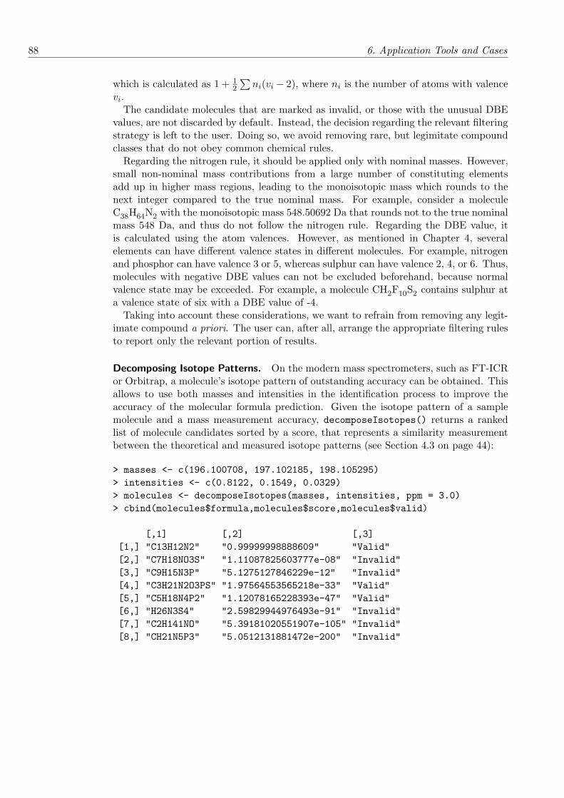
88 6. Application Tools and Cases
which is calculated as 1 + 12
∑ni(vi − 2), where ni is the number of atoms with valence
vi.The candidate molecules that are marked as invalid, or those with the unusual DBE
values, are not discarded by default. Instead, the decision regarding the relevant filteringstrategy is left to the user. Doing so, we avoid removing rare, but legimitate compoundclasses that do not obey common chemical rules.
Regarding the nitrogen rule, it should be applied only with nominal masses. However,small non-nominal mass contributions from a large number of constituting elementsadd up in higher mass regions, leading to the monoisotopic mass which rounds to thenext integer compared to the true nominal mass. For example, consider a moleculeC38H64N2 with the monoisotopic mass 548.50692 Da that rounds not to the true nominalmass 548 Da, and thus do not follow the nitrogen rule. Regarding the DBE value, itis calculated using the atom valences. However, as mentioned in Chapter 4, severalelements can have different valence states in different molecules. For example, nitrogenand phosphor can have valence 3 or 5, whereas sulphur can have valence 2, 4, or 6. Thus,molecules with negative DBE values can not be excluded beforehand, because normalvalence state may be exceeded. For example, a molecule CH2F10S2 contains sulphur ata valence state of six with a DBE value of -4.
Taking into account these considerations, we want to refrain from removing any legit-imate compound a priori. The user can, after all, arrange the appropriate filtering rulesto report only the relevant portion of results.
Decomposing Isotope Patterns. On the modern mass spectrometers, such as FT-ICRor Orbitrap, a molecule’s isotope pattern of outstanding accuracy can be obtained. Thisallows to use both masses and intensities in the identification process to improve theaccuracy of the molecular formula prediction. Given the isotope pattern of a samplemolecule and a mass measurement accuracy, decomposeIsotopes() returns a rankedlist of molecule candidates sorted by a score, that represents a similarity measurementbetween the theoretical and measured isotope patterns (see Section 4.3 on page 44):
> masses <- c(196.100708, 197.102185, 198.105295)> intensities <- c(0.8122, 0.1549, 0.0329)> molecules <- decomposeIsotopes(masses, intensities, ppm = 3.0)> cbind(molecules$formula,molecules$score,molecules$valid)
[,1] [,2] [,3][1,] "C13H12N2" "0.99999998888609" "Valid"[2,] "C7H18NO3S" "1.11087825603777e-08" "Invalid"[3,] "C9H15N3P" "5.1275127846229e-12" "Invalid"[4,] "C3H21N2O3PS" "1.97564553565218e-33" "Valid"[5,] "C5H18N4P2" "1.12078165228393e-47" "Valid"[6,] "H26N3S4" "2.59829944976493e-91" "Invalid"[7,] "C2H141NO" "5.39181020551907e-105" "Invalid"[8,] "CH21N5P3" "5.0512131881472e-200" "Invalid"

6.3 Rdisop 89
[9,] "H20O11" "0" "Valid"
The above listing contains 9 candidate molecules whose monoisotopic masses lie within3.0 ppm from the measured mass of 196.100708 Da. Each candidate can be inspectedon the validity with respect to the nitrogen rule. The true molecule C13H12N2 is clearlyidentified as the top candidate, based on the score of its isotope pattern.
In the mass spectrometry experiment, the measured peak list typically correspondsto some adduct ion, such as [M + H]+ in LC/ESI-MS experiment. In order to obtainthe molecular formula of the actual sample molecule, the adduct can be removed usingsubMolecules() function:
> query <- subMolecules("C5H10NO4", "H")> query$formula
[1] "C5H9NO4"
Similarly, if during the ionisation an in-source fragmenation occurs, the lost fragmentcan be added to the sample molecule using addMolecules() function.
Related Bioconductor Packages. The data from a mass spectrometer is typically ob-tained in the form of a raw machine data. The current release of Bioconductor (version2.4) contains two packages that handle the peak picking of the raw data: MassSpec-Wavelet [33] and XCMS [111]. As the latter contains a wrapper for MassSpecWavelet,we can suggest XCMS to be used to transform the raw data into the input peak listsfor Rdisop. Another package, called CAMERA [120], which is at the time of this writ-ing available only in a Bioconductor development version13, can be used to extract theisotope peaks from the peak lists generated by XCMS.
After the candidate molecular formulas are generated, the results can be furtherqueried in open-access compound databases, including PubChem14 from the NationalCenter for Biotechnology Information (NCBI), and Chemical Entities of Biological In-terest (ChEBI)15, to find out if any information about this compound exists. Note thata match or non-match does not indicate a correct or incorrect formula, but facilitates inthe subsequent validation or structure elucidation steps.
Summary. We have presented Rdisop, a new R package for the identification of themolecular formula of metabolites solely from its accurate mass and isotope pattern asobtained from high resolution mass spectrometers. The efficient algorithm implementa-tions in Rdisop are complemented with the front-end features to perform the subsequentstatistical analysis. The distributions of Rdisop for Unix/Linux and Windows operatingsystems are available under the GNU General Public License (GPL). As other Biocon-ductor packages, Rdisop offers a high level of standardized documentation through thededicated vignette and help pages16.13http://bioconductor.org/packages/devel/bioc/html/CAMERA.html14http://pubchem.ncbi.nlm.nih.gov/15http://www.ebi.ac.uk/chebi/16http://www.bioconductor.org/packages/2.4/bioc/html/Rdisop.html

90 6. Application Tools and Cases
Rdisop fills the need for a simple and efficient tool for experiments in metabolomicson a small scale. For a large scale application, a relevant graphical user interface isan indispensable feature for the successful interpretation of the molecular formulas ofunknown sample fragments. In the next chapter, we address this issue by presentinga standalone program, that complements the efficient computational methods with apowerful graphical user interface for the large scale analysis of MS data.

7 SIRIUS
According to Human Metabolome Project1, there exist about 2 900 common metabolitesthat are detectable in the human body, not accounting for secondary metabolites. Yet,until recently less than 30 % have been identified. Similar is the situation for highereukaryotes: Up to 20 000 metabolites are currently estimated to remain uncharacterizedfor any given organism [41]. This lack of information is mostly due to the high diversityand variability encountered in the metabolome. Consequently, one of the key challengesin metabolomics, analytical chemistry, and other related life sciences is to establish theknowledge of metabolite identity.
As mentioned in the previous chapter, for a small scale application, a multitude ofvarious tools exists for the identification of small molecules. For a large scale analysis ofmetabolomic data, the existing software solutions are mainly concern with the process-ing and storage of the mass spectrometry (MS) data. One of the most recent examplesin this category is MeltDB [87], a web-based program for the preprocessing, annotationand storage of datasets obtained from metabolomic experiments. Other recent solutionsinclude, e.g., TagFinder [78] and mzMine [69]. Whereas the focus of these packages is onthe preprocessing and annotation functionality, the compound identification is mainlyperformed by mass spectral database lookup. Clearly, these methods are confined toidentifying metabolites and chemical compounds that have been included in some refer-ence library. Unlike in evolved genomics and proteomics with a number of existing targetdatabases, the state-of-art in metabolomics is yet under very developmental stage withthe limited number of available databases [28]. Hence, de novo identification solutionsare highly sought. Moreover, the visualization tools often suffer from poor or no supportof computational methods, while the algorithmic tools are usually command line basedand require good understanding of the software environment [86,111].
We have developed a new java-based application SIRIUS (Sum formula Identificationby Ranking Isotope patterns Using mass Spectrometry), which aims at user-orientedsoftware framework for de novo identification of molecular formulas of metabolites us-ing accurate mass spectrometry data. SIRIUS core comprises efficient algorithms forgenerating all elemental compositions for a given mass and error, calculating isotopepatterns for all chemically relevant compositions, and matching and ranking the candi-date molecules against the input spectrum. These computational methods in SIRIUSare combined with a powerful graphical user interface for a fully featured analysis of MSdata. An extensive management system allows simplified data handling, and offers aneasy way to integrate new algorithms and data structures in the application. Througha user-friendly interface, SIRIUS allows user (i) to import datasets in most known mass
1http://www.metabolomics.ca/
91

92 7. SIRIUS
spectrometry file formats, (ii) automatic recognition of molecular ion adducts availablein the input spectrum, (iii) handy visualization of identified molecular formulas andtheir isotope patterns, (iv) customizable export of identification results to common fileformats. For the means of data post-processing, we provide basic functionality to searchfor molecular formulas identified by the algorithm in NCBI PubChem database2.
The remainder of this chapter is organized as follows: we start by describing the sys-tem architecture, and give some technical details on the used libraries. Then, we presenta basic application workflow and outline the cornerstones of the data and analysis prepa-ration. We also give a brief overview of the existing mass spectrometry data formats,and the file formats that are supported by SIRIUS. Finally, we present the applicationfunctionalities for the analysis of algorithm results, including visualization, data export,and searching for molecular formulas in external databases.
7.1 System Architecture
Similar to a typical three-tier application, SIRIUS structure consists of three layers: thepresentation layer, the functional or business logic layer, and the data layer. The pre-sentation layer consists of the graphical user interface (GUI), and is responsible for thedata visualization and processing the user requests to the next, functional layer. Thefunctional logic layer includes the implementations of the algorithms and general utilitycomponents, which can be used at all layers of application. The third layer comprises aset of domain objects (DOs) that represent basic entities used in the problem domain,for which the application is created. Domain objects are typically designed to be madepersistent in a database or flat files, and thus, have to be clearly distinguished fromthe other types of data, such as user interface widgets or algorithm data structures.Separating domain objects from the user interface and algorithms improves the applica-tion scalability and performance. In Figure 7.1, a schematic illustration of the SIRIUSarchitecture is depicted.
7.1.1 Domain Objects
Domain objects typically represent logical entities containing some important informa-tion in the problem domain space [48]. As our problem domain is the identificationof sample molecules using mass spectrometry, the domain objects represent the corre-sponding entities of this domain such as, e.g., chemical elements, compounds, peak listsetc. The diagram of the structure of the domain objects is shown in Figure 7.2.
In general, domain objects should know how to copy and compare themselves to otherdomain objects of the same type. This is of particular importance in the large scaleapplications, as it keeps implementations error free and easily extendable. Since any do-main object can contain references to other domain objects, the copying and comparisonof the whole hierarchical structures can become tedious and error prone. To overcome
2http://pubchem.ncbi.nlm.nih.gov/

7.1 System Architecture 93
Presentationlayer
Functionallayer
Data layer
Domainobjects
Algorithms
GUIVisualization
Web Services
Import
Export
Persist
File
PubChem
DB
File
a) b)
Algorithms:
General Utility Components:
Component Manager
LoggingResource Manager
Desktop Manager
Main Frame Controller
Configuration
Domain Objects Factory
Equaling Hashing Cloning
Mass decomposition
Computing isotope patterns
Scoring candidate formulas
Figure 7.1: a) The three-tier architecture of the SIRIUS framework. b) Schematic rep-resentation of the main SIRIUS components.
this difficulty, any domain object in SIRIUS extends the basic AbstractDomainObjectthat takes the responsibility over the cloning and comparing functionality.AbstractDomainObject has a default implementation of clone(), hashCode(), and
equals() methods using Java Reflection3. To obtain this built-in functionality, theextending class has to only implement getClonePrototype() method and the cloning ofthe collections. If some DO needs a specific implementation, the default behavior of thesemethods can be overridden. Note that this design sets one important requirement on theDOs structure: Domain objects need to form a directed acyclic graph (DAG), otherwisethe default implementations of clone(), hashCode(), and equals() will produce aninfinite recursion and end up with StackOverflowError exception.
All DOs instances have to be created using AbstractDomainObjectFactory. Thisensures that if the implementation of one DO needs to be changed, the other partsof code can remain untouched as long as the new functionality implements the samedomain object interface. This behavior resembles the well known Abstract Factory designpattern [48].
Keeping domain objects as simple as possible enhances the portability, and simplifiestheir integration with the entities from other domains. Thus, domain objects in SIRIUSare realized as Plain Old Java Objects (POJOs). Furthermore, each domain objectshould have a DO interface that abstracts its implementation from other parts of the
3http://java.sun.com/docs/books/tutorial/reflect/

94 7. SIRIUS
Project
- name: String- peaks: List- msSettings: MassSpectrometerSettings- runs: List
Peak
- mass: double- abundance: double
MassSpectrometerSettings
- massError: double- massErrorUnits: String- abundanceError: double- modifications: List
MassSpectrometerModification
- ions: Set- numberMolecules: int- charge: int- type: int- ionMode: String
MultipleElement- amount: int
Element
- symbol: String- name: String- valence: int- isotopes:
IsotopeDistribution
ComposedElement
- sequence: String- dbe: double- elements: List
IsotopeDistribution
- nominalMass: int- peaks: List
Run
- compounds: List- project: Project- algorithmSettings:
AlgorithmSettings
AlgorithmSettings
- alphabet: DecompositionAlphabet- boundaries: AlphabetBoundaries- blowup: double- massPrecisionFull: double- massPrecisionMin: double- abundancePrecisionFull: double- abundancePrecisionMin: double- abundanceCorrection: double
Compound- peaks: List- modifiedCompounds: List
ModifiedCompound- modification: MassSpectrometerModification
- modifiedPeaks: List- candidates: List
ScoredCompoundCandidate- element: Element- distribution: List- scores: List<double>
DecompositionAlphabet
- elements: List
AlphabetBoundaries- min: Map<String, Integer>- max: Map<String, Integer>
*
1
*
1
*
1
* *
1 *
*
*
1*1
*
*
*
*
1
*
*1
1
*
1
1
1
1
1
1
1
*
1
*extends extends
1
Figure 7.2: Overview of the structure of the domain objects in SIRIUS.
functional layer. The DO interfaces are used to make changes in the implementationeasier and faster. Therefore, all algorithms and GUI components should handle onlyinstances typed to these interfaces, not to the actual implementing classes.
7.1.2 Functional Logic Layer
The functional or business logic layer consists of the algorithm implementations and gen-eral utility components that can be used at all application layers, see Figure 7.1. Majoralgorithm implementations in SIRIUS include (i) generating of all elemental decompo-sitions for a given mass and error, (ii) computation of the molecule’s isotope patternfor a given molecular formula, and (iii) scoring the theoretical isotope pattern against agiven measured peak list. Each implementation is clearly encapsulated from other partsallowing the execution of any individual algorithm separately. As algorithms have beendescribed in detail in Chapter 4, here we omit further discussion on their implementa-tions; more details can be found in the documentation to the application programminginterface (API) on the project web page4.
4http://bio.informatik.uni-jena.de/trac/sirius
7.1 System Architecture 95
SIRIUS components are the part of the central functional layer as they can be usedby the top and bottom application layers as well. They include Component Manager,Configuration, Resource Manager, Logging and others, see Figure 7.1. Here, we give abrief introduction to the several basic components, while the description of the remainingunits can be found in the associated API documentation.
Component Manager. Component Manager is the central component in the applica-tion infrastructure. It is responsible for the creation and deletion of other general utilitycomponents at the business logic layer and other layers as well. By keeping the referencesto all existing components, it allows to statically obtain such reference at any level ofthe application. This way, Component Manager acts as a “container” for all other com-ponents. For example, if user is about to create a new domain object, the presentationlayer requests from the Component Manager the reference to the object factory of thecurrent domain, and performs an instantiation.
The initialization of the components in Component Manager is performed in two steps:First, the basic components such as Logging and Configuration, are created. Then, theremaining units are initialized, which by the creation can employ the functionality of thebasic components. For example, if any of the latter initializations fails, the error can betraced back using the Logging component.
Other Utility Components. Configuration component can be used to store variousconfiguration values that are defined at application startup. For the initialization, thecomponent uses the contents of the application configuration XML file that contains alist of configuration key-value pairs. After creation, clients can query the component forthe configuration values giving a corresponding key as a parameter for the query. Thisway, any configuration parameter given at startup ,e.g., the current application versioncan be retrieved from this component.
Clear and verbose logging is vital both for the development and maintenance phaseof any software. The logging responsibility in SIRIUS is handled by the special purposeLogging component, which is built upon a widely used Log4j Library 1.2.145. Log4joffers an extensive functionality for advanced and verbose logging at all applicationlevels. Similar to a typical logging framework, Logging component in SIRIUS dividesthe log output to five different levels: DEBUG, INFO, WARNING, ERROR, FATAL. Note thatthe debug level should be used sparingly, such that at least in production it is completelyleft away from the actual file output. To make the logging available at the presentationlayer, a dedicated Log Panel exists that accumulates the log output and informs userwith notifications.
The component Resource Manager is used to obtain references to any external binaryresources such as images, sounds, videos etc. Each resource used in the application hasits entry in the resource map in Configuration. Using a relevant key, clients can query theResource Manager to provide a Uniform Resource Locator (URL) of the corresponding
5http://logging.apache.org/log4j/

96 7. SIRIUS
resource. One of the basic examples of using the Resource Manager is to provide an iconfile to be shown in the presentation layer.
Another general utility component is a Biological Data Service, which provides anybiochemical data necessary for our analysis, such as the properties of the relevant chem-ical elements that includes, e. g., a distribution of natural isotopes, and valences. Uponthe component creation, this information is initialized from the configuration XML fileusing the XStream Library 1.2.26, which allows a simplified (de-)serialization of XMLfiles, and is used for this task throughout our application. To de-serialize any file intothe application, a Serialization Manager is used, which unmarshalls the contents of thefile available from the hard disk or class loader into the corresponding data structure.Similar, a serialization of any object back to the XML file is performed.
7.1.3 Presentation Layer
The SIRIUS presentation layer consists of the graphical user interface (GUI), which isbased on the standard Java Swing Library7. SIRIUS employs a wide variety of otherSwing-based technologies that can be reused to keep a unified design and simplify theintegration of new functionalities. Here, we only outline several major aspects of the GUIinfrastructure; the remaining parts can be found in the associated API documentation.
Application Desktop. Frames and panels on the application desktop are arranged andmanaged by the docking system of the VLDocking Framework 2.1.48. Using docking, theapplication views can be arranged or docked on the desktop with respect to their respon-sibility, allowing for a simple navigation and customization of the application desktop.Docking of UI components at the SIRIUS application frame is handled by the DesktopManager component. Desktop Manager contains two desktops: a view desktop, whichcorresponds to the full application frame, and a data desktop, which is a segment of theview desktop, and displays the output of the algorithms. Correspondingly, all UI com-ponents are divided in two categories: components that display the algorithm results aregrouped together on the data desktop, while the remaining units are spread around occu-pying the remaining space, and can be toggled on or off depending on the user needs. InFigure 7.4, a typical view of the SIRIUS main frame is shown: views containing the algo-rithm output are tabbed together in the central pane, while other components are placedon the boundaries, including Project Explorer (left), Properties View (left bottom),and Log Panel (bottom). Such layout clearly separates the output of the computa-tional methods from other information, allowing clear navigation and customization ofthe application frame. Adding a new component to the desktop structure is as easy asproviding a component’s unique identifier, a group to which the component belongs, andother supplementary information such as a title and icon.
6http://xstream.codehaus.org/7http://java.sun.com/docs/books/tutorial/uiswing/8http://www.vlsolutions.com/en/index.php

7.1 System Architecture 97
Dialogs and Panels. Dialogs and panels in SIRIUS are based on the JGoodies Forms1.0.79, which provides a powerful and precise layout for the GUI components. Tokeep a standardized look-and-feel, SIRIUS supplies the base classes DefaultDialog andDefaultPanel, which can be extended by newly created GUI components. In addition,UIUtils class provides a set of useful utility functions for the consistent GUI design,including the creation of the default form builders, columns, rows, borders etc.
Wizards. For creation of new projects and analyses, SIRIUS employs Wizard dialogsfrom the SwingLabs Wizard Project (version 0.992)10. An open-source Wizard APIoffers a powerful framework for making the comprehensive wizards by coupling to-gether several settings pages for entering the user input. Although wrapped togetherfor the wizard purposes, the input components in SIRIUS are fully decoupled from theWizard API itself, and can be reused in different from the wizard-based implementa-tions. For example, handling of the algorithm specific parameters is performed on theAlgorithmSettingsPanel, which is used both in a wizard-based creation of each par-ticular analysis and for modifying the default algorithm settings globally.
Application Startup and Shutdown. SIRIUS startup is realized using Swing Appli-cation Framework (SAF) 1.0311, which offers developers a rich set of elements typicalto any Swing-based application, such as lifecycle, session storage, threading and others.SAF has already been successfully integrated in large scale applications for the anal-ysis of phylogenetic [53] data. SIRIUS integrates several SAF features, including theapplication lifecycle and session state functionality.
Each application has a well-defined life cycle, such as launching the application, start-ing the GUI, and shutting down. Each stage has a corresponding method that ourapplication can extend or use the default SAF functionality. For example, SIRIUS over-rides only two methods startup() and shutdown() from the SAF Application class toprovide the specific behavior to the corresponding lifecycle stages, whereas the remainingwork to successfully start and close the application is left to the underlying framework.Upon startup, Application reads the configuration file with application settings thatinclude, e. g., an icon, title, screener, and launches the program. Upon shutdown, vari-ous runtime properties of the application can be stored. These properties can be usedto store small amounts of client specific graphical configuration, including window size,internal frame locations, and other graphical properties. To save this data locally andrestore by the next start, SIRIUS utilizes the session storage functionality of the SAFApplicationContext class.
After starting up SAF default functionally, SIRIUS performs a few more preparationsteps. First, a Component Manager is created, which performs the initialization of alldata layer components, general utilities components, and Desktop Manager. Then, MainFrame Controller is initialized, which, in turn, setups the remaining UI widgets on the
9http://www.jgoodies.com/freeware/forms/10https://wizard.dev.java.net/11https://appframework.dev.java.net/

98 7. SIRIUS
main frame including an icon and main menu. Main Frame Controller is responsiblefor handling all application events coming to the main view. This way, it functions as aController in a Model-View-Controller (MVC) design pattern [44], which is one of thecornerstones of any Swing-based application. Here, we omit further details about theMain Frame Controller. The complete description of this and other components involvedin the application startup can be found in the associated API documentation.
Finally, the application desktop is shown, indicating the readiness of application toreceive and handle user requests. For a “quick start” example, SIRIUS provides somedemo data from the datasets described in Section 4.4. Once this data is uploaded, afew demo projects become available for submission to the identification algorithm. Adetailed survey to the typical application workflow is the topic of the next section.
7.2 Application Workflow
A typical SIRIUS workflow includes the following steps: preparing the input data forthe analysis, setting up and running the algorithm, and analyzing the algorithm results.In this section, we discuss each of these steps in more detail.
7.2.1 Preparing Input Data
A project is a root object in the hierarchy of the SIRIUS domain, and serves as a“portfolio” for the input and output data of the algorithm analysis. Originated from thelaboratory experiment, the input for the computational analysis includes the processedMS data in the form of peak lists, and settings of the mass spectrometer on which thisdata has been obtained. Instrument settings include a mass, an abundance error, and aset of molecular ion adducts typical for this instrument.
In an initial step, the input data has to be added to the project. For an upload of thepeak lists only, user can perform a dedicated Import Data task from the pop-up or filemenu, which reads the MS data from file(s) and adds it to one of the available projects.Alternatively, the input peak lists and machine settings can be entered manually12 in anew project or analysis wizard. The corresponding tasks are, again, available from thepop-up or file menu. After initialization, the input peak list and machine settings canbe reused for multiple analyses within the same project.
To import mass spectrometry data, SIRIUS employs the ProteomeCommons.org IOFramework 6.21 [38], which allows reading most of the available MS data formats. Inthe remainder of this section, we give a short overview of the existing file formats, andprovide recommendations upon conversion of the raw data to file formats supported bySIRIUS.
Supported Mass Spectrometry Data Formats. Following the variety of commercialand custom-build mass spectrometers, a multitude of different MS data formats exists.
12For the peak lists, the file(s) upload is also available.

7.2 Application Workflow 99
All available file formats can be divided into three groups: binary data, plain text, andmore recent XML-based format.
The raw data obtained from a mass spectrometer is stored in a vendor binary fileformat. Several well known binary formats include raw/Xcalibur (Thermo Electron),wiff/Analyst (ABI and MDS Sciex), raw/MassLynx (Waters), and baf (Bruker). Beforecomputational analysis, MS spectra has to be extracted from raw data to ASCII or XMLdata formats. A number of various conversion tools are available for vendor specific fileformats13. Alternatively, the raw data can be converted into a network Common DataForm (netCDF), a binary data format, which is widely used for saving experimental dataincluding MS data14.
Typical examples of the plain text format are mgf (MASCOT), dta (SEQUEST), andpkl (ProteinLynx, Micromass). While saving low resolution or low volume MS data inplain text can be a plausible solution, as far as high resolution or chromatography MSdata is concerned, the usage of ASCII format becomes impractical due to the huge filesize. Moreover, plain text files do not contain precursor scans, thus, lacking valuableinformation for comprehensive computational analysis.
More recently, an open XML file format mzXML [95] has been introduced for stor-ing data generated by mass spectrometry runs, and has been quickly supplied with anumber of tools to convert manufacturer formats, such as Mascot Distiller15, ReAdW,mzBrucker, and others16. However, mzXML has not been designed to contain biologicaldescriptive information. About the same time, the mzData format [90] has been devel-oped with the primary concern of encapsulating the peak lists from raw data, and thedurable archiving of the extracted data in public repositories. As the existence of twoseparate formats for essentially the same purpose has been causing considerable confu-sion and extra programming support, it has been decided to create a new format unifyingmzXML and mzDATA. In June 2009, a joined mzML 1.1.0 format was released underthe guidance of the HUPO Proteomics Standards Initiative (PSI)17, which addresses theproblem of standardizing mass spectrometry-related data formats and vocabulary.
As the importing functionality in our application basically extends the ProteomeCom-mons.org IO Framework, SIRIUS can read all mass spectrometry formats that are sup-ported by this library18. A more detailed list of existing file formats and conversionutilities can be found on the web19.
7.2.2 Analysis Preparation and Parameter Input
After importing the input data, the next step of the SIRIUS application workflow is toset up a new analysis run. To achieve this, user can start a new analysis wizard on theselected project. If no project with relevant data exists, a wizard for the creation of a13http://sashimi.sourceforge.org14http://www.unidata.ucar.edu/software/netcdf/15http://www.matrixscience.com/distiller.html16http://tools.proteomecenter.org/software.php17http://www.psidev.info18http://www.proteomecommons.org/current/531/19http://www.proteomecommons.org,http://tools.proteomecenter.org/software.php

100 7. SIRIUS
new project can be invoked, which also includes the analysis setup. Preparation of anew algorithm run includes the following steps: setting up the algorithm parameters,extracting isotope patterns from the input peak list, and validating the list of compoundsfor the subsequent computational analysis.
Algorithm Parameters. Algorithm parameters include the settings for the mass decom-position algorithm, such as a blowup factor and alphabet (see Section 3.2 on page 31),and for scoring of the isotope patterns (see Section 4.3 on page 44). Furthermore, theuser can specify bounds on the minimal and maximal amount of elements in the candi-date molecule. Often in de novo interpretations of MS data, a partial tag or other samplepreparation information can suggest such constraints. Providing the lower and upperbounds on the number of elements restricts the search space to only relevant candidatemolecules and can significantly speed up the search, see Section 6.1.2 on page 72.
SIRIUS provides the user with reasonable default values for the algorithm parameters.To customize the preferences to his own needs, user can open the Preferences dialogand modify the algorithm settings globally, see Figure 7.3. The applied changes will besaved in the user local workspace and automatically reloaded in any subsequent wizard.
Extracting and Validating Isotope Patterns. To extract isotope patterns, the inputpeak list is parsed and divided into signal groups related to different compounds. A peaklist can also contain several signal groups belonging to the same compound, modifiedby different molecular ion adducts. Typical ion adducts, such as [M + H]+ and [M +Na]+, are provided as a part of the default MS instrument settings, and can be furthercustomized. Identifying modifications is done by calculating mass differences betweenmonoisotopic peak masses. In view of the small number of adducts, we apply a simpleexhaustive search to find all matching mass differences. If there is no prior knowledge onthe source of modification, the user can manually assign one or more adduct types to anisotope pattern. Moreover, if an automatic arrangement of individual peaks to isotopepatterns has failed, each peak can be manually assigned to a proper signal group usinga simple drag-and-drop.
After grouping isotope patterns to compounds, one or more compounds of interest canbe selected for the subsequent identification analysis. Before executing the algorithm, theresults on the approximate number of candidates for each compound can be previewed.To obtain these estimates, we use Equation (3.4) to compute the approximate numberof decompositions for a given mass, error, and alphabet. If the approximate number ofsolutions exceeds a certain customizable threshold, the user receives a notification andcan modify the input before submitting it to the algorithm.
After creation, the analysis is added to the corresponding project, and is shown asits child node in the Project Explorer, see the left pane in Figure 7.4. For the visualinspection of entered data, the contents of each node can be viewed in the Propertiesview, see the left bottom window in Figure 7.4.

7.2 Application Workflow 101
Figure 7.3: The SIRIUS preferences dialog.
7.2.3 Analyzing Algorithm Results
The output of the algorithm is a list of candidate molecular formulas for each compound.Candidates are ranked with respect to the score that reflects the probability that thiscandidate is a true molecular formula for the analyzed compound, see Section 4.3. In theresults view, molecular formulas are listed in the summary table, sorted in decreasingorder of likelihoods. To view an entry in more detail, the user can select and compareseveral theoretical and measured isotope patterns visually.The visual comparison of iso-tope patterns is realized using an open-source JFreeChart Library 1.0.520, which offersan extensive set of functions to create professional quality charts. SIRIUS extends thisrich functionality, e.g., for printing or zooming in the chart for detailed examination ofthe differences between isotope patterns.
Another possibility to analyze the results of the algorithm is to export them to the userworkspace in the form of PDF reports, and open for further evaluation using the defaultsystem or user specified editor. Furthermore, the algorithm results can be exported
20http://www.jfree.org/jfreechart/

102 7. SIRIUS
Figure 7.4: The SIRIUS main frame.
into machine–readable file formats such as plain text and XML documents, that can befurther used as an input in a larger algorithmic pipeline.
Querying Post-processed Data. The candidate molecular formulas can be queried inan open-access NCBI PubChem database to obtain any information available for thecompound with a given molecular formula. The retrieved information can facilitate infurther verification or structure elucidation steps.
PubChem Compound and Substance databases belong to the NCBI Entrez cross-database search system21, which provides a set of tools, Entrez Programming Utilities(eUtils), for the retrieval of Entrez data outside of the regular web query interface. TheNCBI eUtils Web Service22 provides developers an access to eUtils via SOAP protocol.For the short introduction to Web Services, see Section 6.1.2.
For any NCBI Entrez database, a simple search query for one or more molecularformulas can be created using a corresponding database client. SIRIUS employs a sim-ple strategy to search for the compound information: First, the PubChem Compounddatabase is queried, which contains a chemical structural information. If no match isfound, then the PubChem Substance database is searched on the chemical descriptionof the compound. Moreover, the latter can contain the information on the compound
21http://www.ncbi.nlm.nih.gov/sites/gquery22http://www.ncbi.nlm.nih.gov/entrez/query/static/esoap_help.html

7.3 Summary 103
Figure 7.5: Query results to the NCBI PubChem Database.
biological activity. Upon retrieval, the results on putative compounds are shown in thededicated view, see Figure 7.5. Displayed information include a molecule’s name, aCompound ID (CID) or Substance ID (SID), a chemical structure, and other compoundproperties.
7.3 Summary
We have presented SIRIUS, a new java-based software framework for de novo identifi-cation of molecular formulas of metabolites using high-resolution mass spectra. SIRIUSemployes recently developed, efficient computational methods, and combines them with apowerful graphical user interface for the comprehensive analysis of MS data. Well-definedinfrastructure of our application provides a simple way to integrate new computationand visualization functionalities in the framework.
As the focus of our application lies on the computational analysis of MS data, SIRIUS

104 7. SIRIUS
currently supports the export of the analysis results as flat files only. However, aftercontinuous usage of the application, the amount of analyzed data inevitably grows, andsaving this information by means of flat files soon becomes impractical. Therefore, we arecurrently performing further developments to add a database support to our applicationfor the local storage and reuse of the user specific project and analysis data.
Moreover, for execution of particularly memory consuming tasks and for non-interac-tive uses, we are planning to extend SIRIUS to run in the batch processing mode. Forefficient memory usage, any input/output or computationally intensive tasks should beexecuted in a background thread. As our application constantly handles algorithmicallyintensive problems, we would like to enhance current SIRIUS implementations with therich threading functionality of the Swing Application Framework for starting, stopping,and monitoring the progress of background tasks.
SIRIUS is freely available for download at the project website23. SIRIUS distributionsfor various operating systems include Unix/Linux, Windows and Mac OS. Alternatively,the user can deploy and execute the application over the network using Java Web Start24.To run SIRIUS, a Java Runtime Environment (JRE), version 1.5 or newer, is required.Regarding hardware requirements, we recommend at least 256 MB, or better 512 MB offree memory.
To facilitate in further collaborative development, we provide a SIRIUS Trac25, an ex-tensive bug and issue tracking system, which makes the application development processtransparent for the end users, and provides means for an immediate feedback. Follow-ing the SIRIUS Trac, one can (i) examine the list of changes on SIRIUS over the timeline, (ii) learn more about our future plans and milestones looking at the road map,(iii) report a problem or suggestion by creating a new ticket using the guest login, and(iv) view tickets on their resolution state. Finally, SIRIUS Trac includes a completeAPI documentation and a detailed user manual for the guidance to all nuances of theapplication usage.
23http://bio.informatik.uni-jena.de/sirius/24http://java.sun.com/products/javawebstart/25http://bio.informatik.uni-jena.de/trac/sirius

8 Conclusion
In this thesis, we have discussed several algorithms and applications for identification ofsample molecules using high resolution mass spectrometry data.
After the completion of a multitude of various genomes, the bioinformatics research hasprogressed by focusing on the study of different functional levels of biological systemsincluding transcriptome, proteome, and metabolome. These studies allow an under-standing of living organisms at the molecular system level, and provide an insight intothe complex functioning of biological systems.
With the major advances in MS instrumentation, an era of “precision” proteomicshas been recently announced [81]. This implies a routine high-throughput acquisitionof very accurate MS data, such as of several parts-per-million (ppm) mass measurementaccuracy. For metabolomics, this accurate information can greatly facilitate in resolvingits major challenge – the identification of metabolites, whose majority remains unknownto date. So far, this bottleneck has prevented metabolomics to unroll its full potentialin life science. With regards to human health alone, great benefits of metabolomic in-vestigations can be expected: Recent experimental studies have shown the potential ofmetabolomics to provide new biomarkers indicative of human disease [2]. However, incontrast to the emerging fields of genomics and proteomics, the progress in metabolomicsregarding the number of existing computational methods, and applications for the analy-sis of MS data is far from satisfying. Due to the enormous complexity and high dynamicsof the metabolome, the number of available metabolomics databases is limited [28]. Con-sequently, de novo identification solutions are highly sought.
We have presented an algorithm that employs accurate isotopic abundances for iden-tifying the molecular formula of metabolites. Revealing the molecular formula is acrucial step in identifying a metabolite, as it greatly reduces the search space of possiblemolecular structures that can be further examined for automatic structure elucidationof molecules. We have proposed the notion of an isotope pattern, and presented methodsfor the efficient computation of isotope patterns, which is important for the analysis oflarger molecules where the search space increases rapidly. We have evaluated our methodon several datasets obtained from different MS techniques, and achieved results of ex-cellent quality: For orthogonal time-of-flight mass spectrometry, we correctly identifiedmolecular formulas for more than 90 % of the molecules with masses up to 1 000 Da;in other cases the search space was reduced to only a few candidates. Regarding theperformance of our method, it is time and memory efficient and can be executed on acommon desktop computer.
Next, we presented an algorithm to generate all solutions of a multi-dimensional equal-ity constrained integer knapsack problem. This problem arises in the context of findingall amino acid sequences of a peptide with given molecular formula. The results both
105

106 8. Conclusion
on simulated and experimental data demonstrate a superior performance of our mixedmatrix approach which is about two orders of magnitude faster than the second-bestapproach.
Based on the implementations of our algorithms, we have developed several applicationtools that can be used for a small scale analysis of MS data. We have created Decomp,a web-based application for decomposition of integer and real-valued masses over anarbitrary alphabet. Decomp can be applied both for the interpretation of real-valued MSdata and for solving instances of the Money Changing Problem. We have demonstratedthe applicability of our software as a part of another algorithm, called CompNovo, forde novo peptide sequencing using tandem mass spectra. We also have created Rdisop, aR/Bioconductor package for analysis of small sample molecules using an accurate isotopepattern information.
Finally, we have developed the java-based software framework SIRIUS, which imple-ments all the presented algorithms for identification of molecular formulas of metabolites,and combines them with an easy-to-use graphical user interface for the comprehensiveanalysis of MS data. A refined application structure provides a simple way to integratenew computation and visualization methods to the framework. A rich set of SIRIUSpost-processing functionalities, including visualization of isotope patterns, customizabledata export, and searching for molecular formulas in biological databases, is the essentialpart of our software allowing an efficient interpretation of the algorithm results.
Future Work. Although the results computed by our algorithms have achieved a re-markable quality, there are still some unsolved problems.
The current version of our algorithm uses information from only one molecular ionadduct per compound. Combining information from several signal groups belonging tothe same compound (if they exist), could improve identification rates. Since measureddata from different ion adducts of the same compound could be of different quality,our evaluation shows that a simple intersection of candidate lists makes results worse.Instead, a more refined approach is needed. We want to develop a probabilistic modelwhich takes into account the quality of measurements when combining data from multipleadducts. This data can originate from multiply charged ions, so far ignored by ouralgorithm, but upon inclusion, can potentially improve the identification accuracy.
As a more theoretical aspect, one open problem is to improve the approximation ofthe number of decompositions over an alphabet with a considerable number of elements,such as the 20 standard amino acids. This can be achieved by deriving further coefficientsof the polynomial in Equation (3.7) but is far from trivial (Takao Komatsu, personalcommunication).
Regarding our mixed matrix approach for the inference of amino acid compositionfrom a given molecular formula, this work has just started and has further applicationsbeyond the field of proteomics. We are currently conducting evaluations of our methodto compare its performance to other related algorithms such as the one proposed in [93],that solve the general case of a system of linear Diophantine equations with negativecoefficients. Improving existing solutions for the general linear Diophantine systems can

107
have further implications, e.g, for decomposing complex chemical reactions in analyticalchemistry.
Several practical aspects regarding our future work on the SIRIUS software should benoted. SIRIUS is a growing software project, and since its introduction has been subjectto continuous improvement. In release 0.7, called SIRIUS starburst, a novel algorithmfor de novo analysis of metabolites using tandem mass spectra [21] has been integrated,which employs the fragmentation information from several medium-quality mass spectraof the same compound, and searches for the most probable molecular formula thatcan cause the observed fragmentation pattern. In the future SIRIUS releases, we planto integrate other related algorithms such as the one presented in [22], to establish asoftware platform for the comprehensive analysis of metabolites from MS data of varioustypes such as single and tandem mass spectra, fragmentation trees, and others.
Another important aspect of our future work is to evaluate the performance of SIRIUSas an identification tool. We have started addressing this issue by including the func-tionality to search for compounds in the NCBI PubChem database in the current versionof SIRIUS. In future releases, we plan to extend this feature towards fully automatedsearching for molecular formulas in various databases.
We hope that this work is a first step towards the development of efficient compu-tational methods and applications for further discovery and comprehensive analysis ofunknown sample molecules in all species including humans.


Bibliography
[1] K. Aardal and A. K. Lenstra. Hard equality constrained integer knapsacks. In Proc.of Integer Programming and Combinatorial Optimization (IPCO 2002), volume2337 of Lect. Notes Comput. Sc., pages 350–366. Springer, 2002.
[2] B. L. Ackermann, J. E. Hale, and K. L. Duffin. The role of mass spectrometry inbiomarker discovery and measurement. Curr. Drug Metab., 7:525–539, 2006.
[3] R. Aebersold and M. Mann. Mass spectrometry-based proteomics. Nature,422:198–207, 2003.
[4] G. Audi, A. Wapstra, and C. Thibault. The AME2003 atomic mass evaluation(ii): Tables, graphs, and references. Nucl. Phys. A, 729:129–336, 2003.
[5] V. Bafna and N. Edwards. SCOPE: A probabilistic model for scoring tandem massspectra against a peptide database. Bioinformatics, 17:S13–S21, 2001.
[6] N. Bandeira, J. Ng, D. Meluzzi, R. G. Linington, P. Dorrestein, and P. A. Pevzner.De novo sequencing of nonribosomal peptides. In Proc. of Research in Computa-tional Molecular Biology (RECOMB 2008), volume 4955 of Lect. Notes Comput.Sc., pages 181–195. Springer, 2008.
[7] C. Bartels. Fast algorithm for peptide sequencing by mass spectrometry. Biomed.Environ. Mass Spectrom., 19:363–368, 1990.
[8] J. Baumbach. Coryneregnet 4.0 = a reference database for corynebacterial generegulatory networks. BMC Bioinformatics, 8, 2007.
[9] M. Beck, I. M. Gessel, and T. Komatsu. The polynomial part of a restrictedpartition function related to the Frobenius problem. Electron. J. Comb., 8(1):N7,2001.
[10] M. W. Bern and D. Goldberg. EigenMS: De novo analysis of peptide tandem massspectra by spectral graph partitioning. In Proc. of Research in ComputationalMolecular Biology (RECOMB 2005), volume 3500 of Lect. Notes Comput. Sc.,pages 357–372. Springer, 2005.
[11] M. J. Bertrand, P. Thibault, M. J. Evans, and D. Zidarov. Determination ofthe empirical formula of peptides by fast atom bombardment mass spectrometry.Biomed. Environ. Mass Spectrom., 14(6):249–256, 1987.
109

110 Bibliography
[12] A. Bertsch, A. Leinenbach, A. Pervukhin, M. Lubeck, R. Hartmer, C. Baessmann,Y. A. Elnakady, R. Muller, S. Bocker, C. G. Huber, and O. Kohlbacher. De novopeptide sequencing by tandem mass spectrometry using complementary collision-induced dissociation and electron transfer dissociation. Electrophoresis, Jul 2009.Accepted for publication.
[13] R. Bino, R. Hall, O. Fiehn, J. Kopka, K. Saito, J. Draper, B. Nikolau, P. Mendes,U. Roessner-Tunali, M. Beale, R. Trethewey, B. Lange, E. Wurtele, and L. Sum-ner. Potential of metabolomics as a functional genomics tool. Trends Plant Sci.,9(9):418–425, 2004.
[14] S. Bocker. Sequencing from compomers: The puzzle. Theory Comput. Syst.,39(3):455–471, 2006.
[15] S. Bocker, M. Letzel, Zs. Liptak, and A. Pervukhin. Decomposing metabolomicisotope patterns. In Proc. of Workshop on Algorithms in Bioinformatics (WABI2006), volume 4175 of Lect. Notes Comput. Sc., pages 12–23. Springer, 2006.
[16] S. Bocker, M. Letzel, Zs. Liptak, and A. Pervukhin. SIRIUS: Decomposing isotopepatterns for metabolite identification. Bioinformatics, 25(2):218–224, 2009.
[17] S. Bocker, Z. Liptak, M. Martin, A. Pervukhin, and H. Sudek. DECOMP—frominterpreting mass spectrometry peaks to solving the Money Changing Problem.Bioinformatics, 24(4):591–593, 2008.
[18] S. Bocker and Zs. Liptak. Efficient mass decomposition. In L. M. Liebrock, editor,Proc. of ACM Symposium on Applied Computing (ACM SAC 2005), pages 151–157, Santa Fe, USA, 2005. ACM Press.
[19] S. Bocker and Zs. Liptak. A fast and simple algorithm for the Money ChangingProblem. Algorithmica, 48(4):413–432, 2007.
[20] S. Bocker and A. Pervukhin. Inferring peptide composition from molecular for-mulas. In Proc. of Computing and Combinatorics Conference (COCOON 2009),volume 5609 of Lect. Notes Comput. Sc., pages 277–286. Springer, 2009.
[21] S. Bocker and F. Rasche. Towards de novo identification of metabolites by ana-lyzing tandem mass spectra. Bioinformatics, 24:I49–I55, 2008. Proc. of EuropeanConference on Computational Biology (ECCB 2008).
[22] S. Bocker, F. Rasche, and T. Steijger. Annotating fragmentation patterns. InProc. of Workshop on Algorithms in Bioinformatics (WABI 2009), volume 5724of Lect. Notes Comput. Sc., pages 13–24. Springer, 2009.
[23] D. C. Chamrad, G. Korting, K. Stuhler, H. E. Meyer, J. Klose, and M. Bluggel.Evaluation of algorithms for protein identification from sequence databases usingmass spectrometry data. Proteomics, 4:619–628, 2004.

Bibliography 111
[24] T. Chen, M.-Y. Kao, M. Tepel, J. Rush, and G. M. Church. A dynamic program-ming approach to de novo peptide sequencing via tandem mass spectrometry. J.Comput. Biol., 8(3):325–337, 2001.
[25] K. R. Clauser, P. Baker, and A. L. Burlingame. Role of accurate mass measurement(+/- 10 ppm) in protein identification strategies employing MS or MS/MS anddatabase searching. Anal. Chem., 71(14):2871–2882, Jul 1999.
[26] V. Dancık, T. A. Addona, K. R. Clauser, J. E. Vath, and P. A. Pevzner. De novopeptide sequencing via tandem mass spectrometry: A graph-theoretical approach.J. Comput. Biol., 6(3/4):327–342, 1999.
[27] R. Datta and M. Bern. Spectrum fusion: Using multiple mass spectra for de novopeptide sequencing. In Proc. of Research in Computational Molecular Biology (RE-COMB 2008), volume 4955 of Lect. Notes Comput. Sc., pages 140–153. Springer,2008.
[28] K. Dettmer, P. A. Aronov, and B. D. Hammock. Mass spectrometry-basedmetabolomics. Mass Spectrom Rev., 26(1):51–78, 2007.
[29] E. W. Deutsch, H. Lam, and R. Aebersold. Data analysis and bioinformatics toolsfor tandem mass spectrometry in proteomics. Physiological Genomics, 33:18–25,March 2008.
[30] P. A. DiMaggio and C. A. Floudas. De novo peptide identification via tandemmass spectrometry and integer linear optimization. Anal. Chem., 79(4):1433–1446,2007.
[31] Q. Ding, L. Xiao, S. Xiong, Y. Jia, H. Que, Y. Guo, and S. Liu. Unmatchedmasses in peptide mass fingerprints caused by cross-contamination: An updatedstatistical result. Proteomics, 3:1313–1317, 2003.
[32] B. Domon and R. Aebersold. Mass spectrometry and protein analysis. Science,312:212–217, February 2006.
[33] P. Du, W. A. Kibbe, and S. Lin. Improved peak detection in mass spectrum byincorporating continuous wavelet transform-based pattern matching. Bioinformat-ics, 22:2059–2065, 2006.
[34] I. Eidhammer, K. Flikka, L. Martens, and S.-O. Mikalsen. Computational Methodsfor Mass Spectrometry Proteomics. Wiley, 2007.
[35] T. Ejaz, S. Rahmann, and J. Stoye. Online abelian pattern matching. Technical re-port, Bielefeld University, Technische Fakultat der Universitat Bielefeld, AbteilungInformationstechnik, Postfach 10 01 31, 33501 Bielefeld, Germany, January 2008.
[36] J. E. Elias, F. D. Gibbons, O. D. King, F. P. Roth, and S. P. Gygi. Intensity-basedprotein identification by machine learning from a library of tandem mass spectra.Nat. Biotechnol., 22(2):214–219, 2004.
112 Bibliography
[37] J. K. Eng, A. L. McCormack, and J. R. Yates III. An approach to correlate tandemmass spectral data of peptides with amino acid sequences in a protein database.J. Am. Soc. Mass Spectr., 5:976–989, 1994.
[38] J. Falkner, J. Falkner, and P. Andrews. Proteomecommons.org io framework:reading and writing multiple proteomics data formats. Bioinformatics, 23:262–263, 2007.
[39] J. Fenn, M. Mann, C. Meng, S. Wong, and C. Whitehouse. Electrospray ionisationfor mass spectrometry of large biomolecules. Science, 246:64–71, 1989.
[40] D. Fenyo and R. C. Beavis. A method for assessing the statistical significanceof mass spectrometry-based protein identifications using general scoring schemes.Anal. Chem., 75(4):768–774, 2003.
[41] A. R. Fernie, R. N. Trethewey, A. J. Krotzky, and L. Willmitzer. Metaboliteprofiling: from diagnostics to systems biology. Nat. Rev. Mol. Cell Biol., 5(9):763–769, 2004.
[42] O. Fiehn. Metabolomics–the link between genotypes and phenotypes. Plant Mol.Biol., 48(1-2):155–171, 2002.
[43] B. Fischer, V. Roth, F. Roos, J. Grossmann, S. Baginsky, P. Widmayer, W. Gruis-sem, and J. M. Buhmann. NovoHMM: a hidden Markov model for de novo peptidesequencing. Anal. Chem., 77(22):7265–7273, 2005.
[44] M. Fowler. Patterns of Enterprise Application Architecture. Addison-Wesley, 2002.
[45] A. Frank and P. Pevzner. PepNovo: de novo peptide sequencing via probabilisticnetwork modeling. Anal. Chem., 15:964–973, 2005.
[46] A. M. Frank, M. M. Savitski, M. N. Nielsen, R. A. Zubarev, and P. A. Pevzner.De novo peptide sequencing and identification with precision mass spectrometry.J. Proteome Res., 6(1):114–123, September 2007.
[47] A. Furst, J.-T. Clerc, and E. Pretsch. A computer program for the computationof the molecular formula. Chemom. Intell. Lab. Syst., 5:329–334, 1989.
[48] E. Gamma, R. Helm, R. Johnson, and J. Vlissides. Design Patterns. Elements ofReusable Object-Oriented Software. Addison-Wesley, 1994.
[49] L. Y. Geer, S. P. Markey, J. A. Kowalak, L. Wagner, M. Xu, D. M. Maynard,X. Yang, W. Shi, and S. H. Bryant. Open mass spectrometry search algorithm. J.Proteome Res., 3:958–964, 2004.
[50] R. C. Gentleman, V. J. Carey, D. M. B., B. Bolstad, M. Dettling, S. Dudoit,B. Ellis, L. Gautier, Y. Ge, J. Gentry, K. Hornik, T. Hothorn, W. Huber, S. Iacus,R. Irizarry, F. Leisch, C. Li, M. Maechler, A. J. Rossini, G. Sawitzki, C. Smith,

Bibliography 113
G. Smyth, L. Tierney, J. Y. H. Yang, and J. Zhang. BioConductor: Open soft-ware development for computational biology and bioinformatics. Genome Biology,5:R80, 2004.
[51] P. Gilmore and R. Gomory. Multi-stage cutting stock problems of two and moredimensions. Oper. Res., 13(1):94–120, 1965.
[52] A. H. Grange, M. C. Zumwalt, and G. W. Sovocool. Determination of ion andneutral loss compositions and deconvolution of product ion mass spectra usingan orthogonal acceleration time-of-flight mass spectrometer and an ion correlationprogram. Rapid Commun. Mass Spectrom., 20(2):89–102, 2006.
[53] T. Griebel, M. Brinkmeyer, and S. Bocker. EPoS: a modular software frameworkfor phylogenetic analysis. Bioinformatics, 24(20):2399–2400, 2008.
[54] J. Gross. Mass Spectrometry: A textbook. Springer, Berlin, 2004.
[55] W. Haas, B. K. Faherty, S. A. Gerber, J. E. Elias, S. A. Beausoleil, C. E. Bakalarski,X. Li, J. Ville, and S. P. Gygi. Optimization and use of peptide mass measurementaccuracy in shotgun proteomics. Molecular & Cellular Proteomics, 5.7:1326–1337,2006.
[56] M. Hardman and A. A. Makarov. Interfacing the orbitrap mass analyzer to anelectrospray ion source. Anal. Chem., 75(7):1699–1705, 2003.
[57] G. G. Harrigan and R. Goodacre, editors. Metabolic Profiling: Its Role inBiomarker Discovery and Gene Function Analysis. Springer, 2003.
[58] F. He, C. L. Hendrickson, and A. G. Marshall. Baseline mass resolution of peptideisobars: A record for molecular mass resolution. Anal. Chem., 73(3):647–650,2001.
[59] W. J. Henzel, T. M. Billeci, J. T. Stults, S. C. Wong, C. Grimley, and C. Watanabe.Identifying proteins from two-dimensional gels by molecular mass searching ofpeptide fragments in protein sequence databases. Proc. Natl. Acad. Sci. U.S.A.,90(11):5011–5015, 1993.
[60] W. J. Henzel, C. Watanabe, and J. T. Stults. Protein identification: The originsof peptide mass fingerprints. J. Am. Soc. Mass Spectr., 14(9):931–942, 2003.
[61] F. Hillenkamp, M. Karas, R. Beavis, and B. Chait. Matrix-assisted laser desorp-tion/ionization mass spectrometry of biopolymers. Anal. Chem., 63:1193A–1203A,1991.
[62] D. H. Horn, R. A. Zubarev, and F. W. McLafferty. Automated reduction andinterpretation of high resolution electrospray mass spectra of large molecules. J.Am. Soc. Mass Spectr., 11:320–332, 2000.

114 Bibliography
[63] C. S. Hsu. Diophantine approach to isotopic abundance calculations. Anal. Chem.,56(8):1356–1361, 1984.
[64] Y. Iijima, Y. Nakamura, Y. Ogata, K. Tanaka, N. Sakurai, K. Suda, T. Suzuki,H. Suzuki, K. Okazaki, M. Kitayama, S. Kanaya, K. Aoki, and D. Shibata. Metabo-lite annotations based on the integration of mass spectral information. Plant J.,54(5):949–962, Jun 2008.
[65] P. Jones, R. G. Cote, L. Martens, A. F. Quinn, C. F. Taylor, W. Derache, H. Her-mjakob, and R. Apweiler. PRIDE: a public repository of protein and peptideidentifications for the proteomics community. Nucleic Acids Res., 34(Database-Issue):659–663, 2006.
[66] M. Kanehisa, S. Goto, M. Hattori, K. F. Aoki-Kinoshita, M. Itoh, S. Kawashima,T. Katayama, M. Araki, and M. Hirakawa. From genomics to chemical genomics:new developments in KEGG. Nucleic Acids Res., 34:D354–D357, 2006.
[67] E. A. Kapp, F. Schutz, L. M. Connolly, J. A. Chakel, J. E. Meza, C. A. Miller,D. Fenyo, J. K. Eng, J. N. Adkins, G. S. Omenn, and R. J. Simpson. An evaluation,comparison, and accurate benchmarking of several publicly available ms/ms searchalgorithms: Sensitivity and specificity analysis. Proteomics, 5:3475–3490, 2005.
[68] M. Karas and F. Hillenkamp. Laser desorption ionization of proteins with molec-ular masses exceeding 10,000 Daltons. Anal. Chem., 60:2299–2301, 1988.
[69] M. Katajamaa, J. Miettinen, and M. Oresic. Mzmine: toolbox for processing andvisualization of mass spectrometry based molecular profile data. Bioinformatics,22(5):634–636, 2006.
[70] H. Kellerer, U. Pferschy, and D. Pisinger. Knapsack Problems. Springer, 2004.
[71] S. Kim, N. Gupta, and P. A. Pevzner. Spectral probabilities and generating func-tions of tandem mass spectra: a strike against decoy databases. J. Proteome Res.,7(8):3354–3363, 2008.
[72] T. Kind and O. Fiehn. Metabolomic database annotations via query of elemen-tal compositions: Mass accuracy is insufficient even at less than 1 ppm. BMCBioinformatics, 7(1):234, Apr 2006.
[73] T. Kind and O. Fiehn. Seven golden rules for heuristic filtering of molecularformulas obtained by accurate mass spectrometry. BMC Bioinformatics, 8:105,2007.
[74] T. Komatsu. On the number of solutions of the diophantine equation of frobenius- general case. Mathematical Communications, 8:195–206, 2003.
[75] H. Kubinyi. Calculation of isotope distributions in mass spectrometry: A trivialsolution for a non-trivial problem. Anal. Chim. Acta, 247:107–119, 1991.

Bibliography 115
[76] E. Lange, C. Gropl, K. Reinert, O. Kohlbacher, and A. Hildebrandt. High-accuracypeak picking of proteomics data using wavelet techniques. In Proc. of PacificSymposium on Biocomputing (PSB 2006), pages 243–254, 2006.
[77] Zs. Liptak. Strings in Proteomics and Transcriptomics. Algorithmic and Combi-natorial Questions in Mass Spectrometry and EST Clustering. PhD thesis, Uni-versitat Bielefeld, Bielefeld, Germany, May 2005.
[78] A. Luedemann, K. Strassburg, A. Erban, and J. Kopka. TagFinder for the quanti-tative analysis of gas chromatography–mass spectrometry (GC-MS)-based metabo-lite profiling experiments. Bioinformatics, 24(5):732–737, Mar 2008.
[79] G. S. Lueker. Two NP-complete problems in nonnegative integer programming.Technical Report TR-178, Department of Electrical Engineering, Princeton Uni-versity, March 1975.
[80] M. Mann, P. Hojrup, and P. Roepstorff. Use of mass spectrometric molecularweight information to identify proteins in sequence databases. Biol. Mass Spec-trom., 22(6):338–345, 1993.
[81] M. Mann and N. L. Kelleher. Precision proteomics: The case for high resolutionand high mass accuracy. PNAS, 105(47):18132–18138, November 2008.
[82] S. Martello and P. Toth. Knapsack Problems: Algorithms and Computer Imple-mentations. John Wiley & Sons, Chichester, 1990.
[83] L. McHugh and J. W. Arthur. Computational methods for protein identificationfrom mass spectrometry data. PLoS Comput. Biol., 4(2):e12, February 2008.
[84] J. S. Morris, K. R. Coombes, J. Koomen, K. A. Baggerly, and R. Kobayashi.Feature extraction and quantificatioon for mass spectrometry in biomedical appli-cations using the mean spectrum. Bioinformatics, 21(9):1764–1775, 2005.
[85] A. I. Nesvizhskii, O. Vitek, and R. Aebersold. Analysis and validation of proteomicdata generated by tandem mass spectrometry. Nature Methods, 4(10):787–797,September 2007.
[86] S. Neumann, A. Pervukhin, and S. Bocker. Mass decomposition with the Rdisoppackage, October 13 2007. Part of BioConductor 2.2.
[87] H. Neuweger, S. P. Albaum, M. Dondrup, M. Persicke, T. Watt, K. Niehaus,J. Stoye, and A. Goesmann. MeltDB: a software platform for the analysis andintegration of metabolomics experiment data. Bioinformatics, 24(23):2726–2732,2008.
[88] S. Ojanpera, A. Pelander, M. Pelzing, I. Krebs, E. Vuori, and I. Ojanpera. Iso-topic pattern and accurate mass determination in urine drug screening by liquidchromatography/time-of-flight mass spectrometry. Rapid Commun. Mass Spec-trom., 20(7):1161–1167, 2006.

116 Bibliography
[89] J. V. Olsen, L. M. F. de Godoy, G. Li, B. Macek, P. Mortensen, R. Pesch,A. Makarov, O. Lange, S. Horning, and M. Mann. Parts per million mass ac-curacy on an orbitrap mass spectrometer via lock mass injection into a c-trap.Molecular & Cellular Proteomics, 4:2010–2021, 2006.
[90] S. Orchard, L. Montechi-Palazzi, E. W. Deutsch, P.-A. Binz, A. R. Jones, N. Paton,A. Pizarro, D. M. Creasy, J. Wojcik, and H. Hermjakob. Five years of progress inthe standardization of proteomics data 4th annual spring workshop of the hupo-proteomics standards initiative. Proteomics, 7:3436–3440, 2007.
[91] P. M. Palagi, P. Hernandez, D. Walther, and R. D. Appel. Proteome informatics i:Bioinformatics tools for processing experimental data. Proteomics, 6:5435–5444,2006.
[92] T. Palzkill. Proteomics. Kluver Academic Publishers, 2002.
[93] D. Papp and B. Vizvari. Effective solution of linear diophantine equation systemswith an application in chemistry. J. Math. Chem., 39(1):15–31, 2006.
[94] D. J. Pappin, P. Hojrup, and A. Bleasby. Rapid identification of proteins bypeptide-mass fingerprinting. Curr. Biol., 3(6):327–332, 1993.
[95] P. G. A. Pedrioli, J. K. Eng, R. Hubley, M. Vogelzang, E. W. Deutsch, B. Raught,B. Pratt, E. Nilsson, R. H. Angeletti, R. Apweiler, K. Cheung, C. E. Costello,H. Hermjakob, S. Huang, R. K. Julian, E. Kapp, M. E. McComb, S. G. Oliver,G. Omenn, N. W. Paton, R. Simpson, R. Smith, C. F. Taylor, W. Zhu, andR. Aebersold. A common open representation of mass spectrometry data and itsapplication to proteomics research. Nat. Biotechnol., 22(11):1459–66, 2004.
[96] V. Pellegrin. Molecular formulas of organic compounds: the nitrogen rule anddegree of unsaturation. J. Chem. Educ., 60(8):626–633, 1983.
[97] D. N. Perkins, D. J. Pappin, D. M. Creasy, and J. S. Cottrell. Probability-basedprotein identification by searching sequence databases using mass spectrometrydata. Electrophoresis, 20(18):3551–3567, 1999.
[98] S. Pillai, V. Silventoinen, K. Kallio, M. Senger, S. Sobhany, J. Tate, S. Velankar,A. Golovin, K. Henrick, P. Rice, P. Stoehr, and R. Lopez. Soap-based servicesprovided by the european bioinformatics institute. Nucleic Acids Res., 33(WebSever issue):W25–W28, 2005.
[99] S. C. Pomerantz, J. A. Kowalak, and J. A. McCloskey. Determination of oligonu-cleotide composition from mass spectromectrically measured molecular weight. J.Am. Soc. Mass Spectrom., 4:204–209, 1993.
[100] A. L. Rockwood and S. L. Van Orden. Ultrahigh-speed calculation of isotopedistributions. Anal. Chem., 68:2027–2030, 1996.
Bibliography 117
[101] A. L. Rockwood, J. R. Van Orman, and D. V. Dearden. Isotopic compositionsand accurate masses of single isotopic peaks. J. Am. Soc. Mass Spectr., 15:12–21,2004.
[102] S. Rogers, R. A. Scheltema, M. Girolami, and R. Breitling. Probabilistic assign-ment of formulas to mass peaks in metabolomics experiments. Bioinformatics,25(4):512–518, 2009.
[103] M. S. Sabatine, E. Liu, D. A. Morrow, E. Heller, R. McCarroll, R. Wiegand,G. F. Berriz, F. P. Roth, and R. E. Gerszten. Metabolomic identification of novelbiomarkers of myocardial ischemia. Circulation, 112:3868–3865, 2005.
[104] A. Salomaa. Counting (scattered) subwords. B. Euro. Assoc. Theo. Comp. Sci.,81:165–179, 2003.
[105] M. M. Savitski, M. L. Nielsen, F. Kjeldsen, and R. A. Zubarev. Proteomics-gradede novo sequencing approach. J. Proteome Res., 4:2348–2354, 2005.
[106] S. Schneiker, O. Perlova, O. Kaiser, K. Gerth, A. Alici, M. O. Altmeyer, D. Bar-tels, T. Bekel, S. Beyer, E. Bode, H. B. Bode, C. J. Bolten, J. V. Choudhuri,S. Doss, Y. A. Elnakady, B. Frank, L. Gaigalat, A. Goesmann, C. Groeger,F. Gross, L. Jelsbak, L. Jelsbak, J. Kalinowski, C. Kegler, T. Knauber, S. Koni-etzny, M. Kopp, L. Krause, D. Krug, B. Linke, T. Mahmud, R. Martinez-Arias,A. C. McHardy, M. Merai, F. Meyer, S. Mormann, J. Munoz-Dorado, J. Perez,S. Pradella, S. Rachid, G. Raddatz, F. Rosenau, C. Ruckert, F. Sasse, M. Scharfe,S. C. Schuster, G. Suen, A. Treuner-Lange, G. J. Velicer, F.-J. Vorholter, K. J.Weissman, R. D. Welch, S. C. Wenzel, D. E. Whitworth, S. Wilhelm, C. Wittmann,H. Blocker, A. Pohler, and R. Muller. Complete genome sequence of the myxobac-terium sorangium cellulosum. Nat. Biotechnol., 25(11):1281–1289, 2007.
[107] J. Senior. Partitions and their representative graphs. Am. J. Math., 73(3):663–689,1951.
[108] M. W. Senko, C. L. Hendrickson, and M. R. Emmet. External accumulation ofions for enhanced electrospray ionization fourier transform ion cyclotron resonancemass spectrometry. JASMS, 8:970–976, 1997.
[109] I. Shadforth, D. Crowther, and C. Bessant. Protein and peptide identificationalgorithms using ms for use in high-throughput, automated pipelines. Proteomics,5:4082–4095, 2005.
[110] G. Siuzdak. Mass Spectrometry for Biotechnology. Academic Press, 1996.
[111] C. A. Smith, E. J. Want, G. O’Maille, R. Abagyan, and G. Siuzdak. XCMS:Processing mass spectrometry data for metabolite profiling using nonlinear peakalignment, matching, and identification. Anal. Chem., 78(3):779–787, Feb 2006.

118 Bibliography
[112] R. D. Smith, G. A. Anderson, M. S. Lipton, L. Pasa-Tolic, Y. Shen, T. P. Conrads,T. D. Veenstra, and H. R. Udseth. An accurate mass tag strategy for quantitativeand high-throughput proteome measurements. Proteomics, 2:513–523, 2002. Issue5.
[113] A. P. Snyder. Interpreting Protein Mass Spectra: A Comprehensive Resource.Oxford University Press, 2000.
[114] M. D. Soffer. The molecular formula generalized in terms of cyclic elements ofstructure. Science, 127(3303):880, April 1958.
[115] B. Spengler. De novo sequencing, peptide composition analysis, and composition-based sequencing: A new strategy employing accurate mass determination byfourier transform ion cyclotron resonance mass spectrometry. J. Am. Soc. MassSpectrom., 15(5):703–714, 2004.
[116] M. Sturm, A. Bertsch, C. Gropl, A. Hildebrandt, R. Hussong, E. Lange, N. Pfeifer,O. Schulz-Trieglaff, A. Zerck, K. Reinert, and O. Kohlbacher. Openms - an open-source software framework for mass spectrometry. BMC Bioinformatics, 9:163,2008.
[117] J. E. P. Syka, J. J. Coon, M. J. Schroeder, J. Shabanowitz, and D. F. Hunt. Peptideand protein sequence analysis by electron transfer dissociation mass spectrometry.Proc. Natl. Acad. Sci. U.S.A., 101(26):9528–9533, 2004.
[118] S. Tanner, S. H. Payne, S. Dasari, Z. Shen, P. A. Wilmarth, L. L. David, W. F.Loomis, S. P. Briggs, and V. Bafna. Accurate annotation of peptide modificationsthrough unrestrictive database search. J. Proteome Res., 7:170–181, 2008.
[119] S. Tanner, H. Shu, A. Frank, L.-C. Wang, E. Zandi, M. Mumby, P. A. Pevzner,and V. Bafna. Inspect: Identification of posttranslationally modified peptides fromtandem mass spectra. Anal. Chem., 77:4626–4639, 2005.
[120] R. Tautenhahn, C. Bottcher, and S. Neumann. Annotation of lc/esi-ms mass sig-nals. In Proc. of Conference on Bioinformatics Research and Development (BIRD2007), volume 4414 of Lect. Notes Comput. Sc. Springer, 2007.
[121] J. A. Taylor and R. S. Johnson. Sequence database searches via de novo pep-tide sequencing by tandem mass spectrometry. Rapid Commun. Mass Spectrom.,11:1067–1075, 1997.
[122] J. A. Taylor and R. S. Johnson. Implementation and uses of automated de novopeptide sequencing by tandem mass spectrometry. Anal. Chem., 73:2594–2604,2001.
[123] J. van Lint and R. Wilson. A Course in Combinatorics. Cambridge UniversityPress, 2001.

Bibliography 119
[124] S. M. Watkins and J. B. German. Toward the implementation of metabolomicassessments of human health and nutrition. Curr. Opin. Biotechnol., 13(5):512–516, October 2002.
[125] J. T. Watson and O. D. Sparkman. Introduction to Mass Spectrometry: Instru-mentation, Applications, and Strategies for Data Interpretation. Wiley, 2007.
[126] C. Whitehouse, R. Dreyer, M. Yamashita, and J. Fenn. Electrospray interface forliquid chromatographs and mass spectrometers. Anal. Chem., 57:675–679, 1985.
[127] H. Wilf. generatingfunctionology. Academic Press, 1990.
[128] C. Yang, Z. He, and W. Yu. Comparison of public peak detection algorithms formaldi mass spectrometry data analysis. BMC Bioinformatics, 10(4), 2009.
[129] J. R. Yates III, J. K. Eng, A. L. McCormack, and D. Schieltz. Method to correlatetandem mass spectra of modified peptides to amino acid sequences in the proteindatabase. Anal. Chem., 67(8):1426–1436, 1995.
[130] J. R. Yates III, S. Speicher, P. R. Griffin, and T. Hunkapillar. Peptide massmaps: A highly informative approach to protein identification. Anal. Biochem.,214:397–408, 1993.
[131] J. A. Yergey. A general approach to calculating isotopic distributions for massspectrometry. Int. J. Mass Spectrom. Ion Phys., 52(2–3):337–349, 1983.
[132] J. Zhang, W. Gao, J. Cai, S. He, R. Zeng, and R. Chen. Predicting molecular for-mulas of fragment ions with isotope patterns in tandem mass spectra. IEEE/ACMTrans. Comput. Biol. Bioinform., 2(3):217–230, 2005.
[133] N. Zhang, R. Aebersold, and B. Schwikowski. ProbID: a probabilistic algorithm toidentify peptides through sequence database searching using tandem mass spectraldata. Proteomics, 2(10):1406–1412, Oct 2002.
[134] W. Zhang and B. T. Chait. ProFound: an expert system for protein identificationusing mass spectrometric peptide mapping information. Anal. Chem., 72(11):2482–2489, 2000.
[135] Z. Zhang. De novo peptide sequencing based on a divide-and-conquer algorithmand peptide tandem spectrum simulation. Anal. Chem., 76:6374–6383, 2004.
[136] R. A. Zubarev, N. L. Kelleher, and F. W. McLafferty. Electron capture dissocia-tion of multiply charged protein cations. a nonergodic process. J Am Chem Soc,120:3265–3266, 1998.