Molecular Dynamics Simulations of the Liquid/Vapor Interface of Aqueous EthanolSolutions as a Function of Concentration

Ethan Stewart, Roseanne L. Shields, and Ramona S. Taylor*

Department of Chemistry, College of the Holy Cross, Worcester, Massachusetts 01610

ReceiVed: October 4, 2002; In Final Form: January 7, 2003

Molecular dynamics computer simulations are utilized to study the structural and thermodynamic propertiesof the liquid/vapor interface of aqueous ethanol solutions as a function of concentration. In addition, the freeenergy profile for inserting a single ethanol molecule into a 0.059 mole fraction aqueous ethanol solution iscalculated using statistical mechanical perturbation theory. The calculated free energy for solvation of anethanol molecule in the bulk solution, the surface tension as a function of ethanol concentration, and theaverage orientation of ethanol molecules at the solution/vapor interface are in agreement with the correspondingexperimental data. The calculated equilibrium free-energy profile, however, exhibits a barrier to solvationthat is considerably smaller than that predicted by the resistance model for mass accommodation.

I. Introduction

Liquid/vapor interfaces play a key role in many biological,chemical, materials, and environmental processes. For example,gas/liquid interfaces are integral to environmental problems suchas the generation of tropospheric ozone, the formation of cloudcondensation nuclei, the depletion of stratospheric ozone, waterpollution, and acid rain deposition.1 Due to its intrinsicasymmetry and two-dimensionality, the interface between twobulk systems typically has different chemical and physicalproperties than either of the bulk systems. It is often morereactive than either bulk medium. It can enhance or impede theoccurrence of chemical reactions, and it can mediate the transferof chemical species between the two bulk systems. Thestructures of liquid interfaces are much more sensitive to thepresence of adsorbed molecules than solid interfaces. Thus, totruly understand how liquid interfaces participate in variouschemical processes, we need a molecular-level understandingof those types of forces that dictate the underlying structure ofthe interface.

The solution/vapor interfaces of aqueous solutions have longbeen the subject of chemical study. In the early 20th century,surface tension measurements of aqueous alcohol solutionsrevealed that the alcohol molecules were surface active.2,3

Today, direct insight into the microscopic structures of thealcohol solution/vapor interface is available via sum frequencygeneration (SFG) and second harmonic generation (SHG)spectroscopies.4-7 For example, using SFG, Wolfrum and co-workers measured an excess density of methanol molecules atthe solution/vapor interface of aqueous methanol solutions.7

They found that the molecular ordering of the surface methanolmolecules increased as the overall concentration of methanoldecreased.7 Neutron reflectivity measurements provide detailsinto the macroscopic structure of the alcohol-H2O solution/vapor interface.8 Li and co-workers have measured the densityprofiles of both the ethanol and H2O molecules along the normalto the interface for aqueous ethanol solutions with ethanol molefractions below 0.24.8 In addition, they determined both thesurface excess of ethanol molecules and the width of this excess.

Classical dynamics simulations are also commonly used toprobe the structure of the liquid/vapor interface.9-19 Theinformation garnered from these types of calculations iscomplementary to the experimental data described above.Simulations allow one to “see” the structures both of theadsorbed molecules and of the underlying liquid substrate. Inthe early 1990s, Matsumoto and co-workers performed an indepth study of the solution/vapor interface of aqueous methanolsolutions as a function of concentration.10 In agreement withexperiment, this work suggested that methanol preferentiallyadsorbs at the solution/vapor interface at all methanol concentra-tions.10 However, uncertainty existed regarding the actualmolecular composition of the surface region in the concentrationrange of 0.2 to 0.5 mole fraction of methanol. In 1996, Tarek,Tobias, and Klein examined the structural and hydrogen bondingproperties of the interface for a 0.1 mole fraction aqueousethanol solution via molecular dynamics (MD) simulations.13

They, too, observed the segregation of the alcohol molecules,in this case ethanol, toward the liquid/vapor interface. However,no attempt was made to study the structure of the liquid/vaporinterface as a function of bulk ethanol concentration. Mountainexamined the composition profiles for the solution/vaporinterface of aqueous acetonitrile solutions as a function ofconcentration.18 In all cases, acetonitrile was also found to besurface active. Benjamin investigated the thermodynamics,structural, and dynamic properties of the H2O/DMSO solution/vapor interface as a function of DMSO concentration.12

Although DMSO is a very different molecule than either ethanolor methanol, it again segregated toward the liquid/vaporinterface. This segregation, however, was not as substantial asthat observed for ethanol. In addition, Benjamin found anenhancement in the fraction ofgoodhydrogen bonds per H2Omolecule as the interface was approached. This enhancementwas more pronounced for the 0.05 mole fraction DMSO solutionthan for the 0.20 mole fraction solution. Given the differencesin the chemical nature of DMSO and ethanol, it will beinteresting to see if this enhancement of the H2O-H2O hydrogenbonds also occurs in aqueous ethanol solutions.

Aqueous alcohol interfaces have also been useful in advancingour understanding of the process of mass accommodation.14-16,20,21* Corresponding author. E-mail: rtaylor@holycross.edu.

2333J. Phys. Chem. B2003,107,2333-2343

10.1021/jp0271357 CCC: $25.00 © 2003 American Chemical SocietyPublished on Web 02/13/2003

The interaction of small gas-phase molecules with the liquid/vapor interface of aqueous droplets and their subsequentaccommodation into the bulk of the droplet is an integral partof many atmospheric processes.21 Experimental investigationsinto mass accommodation predict that the impinging moleculemust cross a large energy barrier before becoming solvated, oraccommodated, in the bulk liquid.21 In past work, we have usedMD computer simulations to examine the origin of this barrierby simulating the accommodation of a single ethanol moleculeby a H2O droplet.14,15 However, within the constraints of theexperimentally derived resistance model,21 we were unable toreproduce the experimental results. One assumption of theresistance model is that the impinging molecule interacts witha cleanH2O surface.21 Our simulations and the recent experi-ments of Donaldson and Anderson22 question if this is in factthe case. Thus, here we are asking what happens if the impingingethanol molecule is forced to cross an adsorbed ethanol filmbefore becoming solvated within the bulk H2O.

In this work, we have used the OPLS all-atom (OPLS/AA)potential function for ethanol26 and the extended simple pointcharge (SPC/E) potential for H2O23 in conjunction with MDcomputer simulations to explore both the structural and ther-modynamic properties of the solution/vapor interface of aqueousethanol solutions as a function of ethanol concentration. Theaccuracy of any classical simulation is limited by the accuracyof the interaction potential functions employed. Potentialfunctions are available that reproduce many of the bulkproperties of pure ethanol and of pure water. Yet, the ability ofthese potentials to reproduce the interfacial properties of ethanol/water solutions remains undetermined. Comparisons of oursimulation data to the corresponding experimental data suggestthat the combination of the OPLS/AA and SPC/E potentialsboth qualitatively and quantitatively describes the thermody-namic and structural properties of the solution/vapor interfaceof aqueous ethanol solutions. We have also investigated thehydrogen bonding structure of both ethanol and H2O moleculesas a function of their distance from the interface. Unlike theDMSO work of Benjamin,12 we see no concentration effect onthe fraction ofgoodhydrogen bonds between H2O moleculesas a function of distance from the interface. Finally, statisticalmechanical perturbation theory32,33is used to calculate the free-energy profile for inserting an ethanol molecule into a 0.059mole fraction aqueous ethanol solution. This free-energy profiledoes not exhibit the barrier to bulk solvation that is predictedby the resistance model.

II. Method

A. Potential Model. The H2O model employed in thesecalculations is the rigid SPC/E water potential developed byBerendsen and co-workers.23 This potential has been shown toadequately reproduce the surface tension and structural proper-ties of the H2O liquid/vapor interface.24,25 The all-atom OPLS(OPLS/AA) potential of Jorgensen is used to model theinteractions between ethanol molecules.26 Both of these potentialmodels treat the intermolecular interactions via the combinationof a Lennard-Jones 6-12 and a Coulomb potential:

where rij is the distance between atomsi and j in differentmolecules,qi is the charge assigned to atomi, andσij and εij

are the Lennard-Jones parameters. The parameters for the SPC/Eand OPLS/AA potentials are given in Table 1. The intermo-

lecular alcohol-H2O parameters are determined by the Lorentz-Bertholot mixing rules.27

The OPLS/AA potential is a flexible potential that accountsfor both the bond stretching, angle bending and torsionalinteractions. The bond stretching and bending potentials aretreated harmonically. The torsional interactions are determinedfrom the following Fourier series:

Here,φi is the dihedral angle,V1, V2, andV3 are the Fouriercoefficients, andf1, f2, andf3 are the phase angles. The totaltorsional energy is a sum of the torsional energies originatingfrom each torsional anglei.

Because the mass accommodation experiments predict theaccumulation of only a very small concentration of ethanol inthe bulk of the droplet,20,21 we have chosen to investigateaqueous ethanol solutions with less than 0.50 mole fractionethanol concentration. We have collected surface tension,structural and dynamical data for four ethanol/water solutions.These solutions, which are described in Table 2, have ethanolmole fractions (øethanol) of 0.026, 0.059, 0.11, and 0.40. Eachsolution is prepared by randomly replacing H2O molecules inan equilibrated box of SPC/E H2O with ethanol molecules togive the desired ethanol mole fraction. The newly created bulkaqueous ethanol solution is then equilibrated for 200 ps in aNPT ensemble with a pressure of 1 atm. After the bulkequilibration process is complete, thez dimension of the box isincreased by a factor of 3 (as shown in Figure 1) and the newsystem is equilibrated for an additional 500 ps in a NVTensemble with no pressure monitoring. Thezdimension is nowthe direction perpendicular to the two newly created solutionliquid/vapor interfaces. Thex, y, andzdimensions of these fourequilibrated aqueous ethanol solutions, and of a pure ethanolsystem, are given in Table 2.

No data analysis is performed before the initial 500 psequilibration is completed. For the surface tension measure-ments, 10 50 ps trajectories are run in which the data is collectedand analyzed. At each concentration, these 10 surface tensionvalues are averaged to give the reported value. After these 10

U(rij) ) 4εij [(σij

rij)12

- (σij

rij)6] +

qi qj

rij(1)

TABLE 1: Intermolecular Lennard-Jones and CoulombParameters for SPC/E Water23 and OPLS/AA Ethanol26

atom type σ (Å) ε (kcal/mol) q (au)

H (water) 0 0 +0.4238O (water) 3.166 0.1554 -0.8476H (alcohol) 0 0 +0.418O (alcohol) 3.120 0.170 -0.683C (methylene) 3.50 0.066 +0.145C (methyl) 3.50 0.066 -0.180H (alkyl) 2.50 0.030 +0.060

TABLE 2: Summary of System Sizes

ethanol molefraction(øethanol)

no. of watermolecules

no. of ethanolmolecules x× y × z (Å3)

0.026 1485 40 36.30× 36.30× 108.900.059 1285 80 35.87× 35.87× 107.610.11 1029 130 34.86× 34.86× 104.580.40 1260 825 48.73× 48.73× 146.191.00 0 488 36.21× 36.21× 108.63

Utor ) ∑i

{V1i

2[1 + cos(φi + f1i)] +

V2i

2[1 - cos(2φi + f2i)] +

V3i

2[1 + cos(3φi + f3i)]} (2)

2334 J. Phys. Chem. B, Vol. 107, No. 10, 2003 Stewart et al.

trajectories, a 100 ps and a subsequent 200 ps trajectory arerun during which the density profiles, orientational, andhydrogen bonding analyses are completed. The results of thesetwo trajectories are compared to ensure that the calculated valuesare truly equilibrium values.

All of the molecular dynamics simulations are performedusing a modified version of the AMBER 4.0 suite of programs.28

AMBER 4.0 utilizes a Verlet integrator29 to solve the equationsof motion. A step size of 0.001 ps is employed. The temperatureof the simulation cells is maintained at 298 K via the Berendsenscheme30 with a coupling constant of 0.2. All of the bond lengthsin both H2O and ethanol are constrained via the SHAKEalgorithm.31 However, in the ethanol molecules, neither the bondangles nor the torsional angles are constrained. All simulationsutilize a cutoff distance of 11 Å.

B. Potential of Mean Force.The free-energy curve for theinsertion of an ethanol molecule into a 0.059 mole fractionethanol solution is calculated using the thermodynamic pertur-bation approach.32,33Statistical mechanical perturbation theoryhas been widely used to calculate the potential of mean force(PMF) for the association of two entities in a bath of solventmolecules.15,19,34,35The PMF provides a means to quantify theeffect of the bath molecules on the intermolecular interactionof two entities along a reaction coordinate. Here, we have chosenthe reaction coordinate to be the distance along thezdimensionbetween the centers of mass of a single impinging ethanolmolecule and of the box of ethanol and water molecules thatconstitute the 0.059 mole fraction aqueous ethanol solution. Thisis a similar approach to that which was utilized in our earlierwork, which investigated the free energy for the insertion of asingle ethanol molecule into bulk water.14,15

The difference in the calculated free energies between twosuccessive steps along the reaction coordinate is equal to thereversible work,W(z), for this configurational change in thepresence of the bath. The relative free-energy difference betweentwo configurations is calculated as follows:

whereT is the temperature of the system. The difference in theHelmholtz free energies,∆A, is calculated between a reference

system,z0, and a system where the reaction coordinate isperturbed fromz0 to (z0 + ∆z). U(z0) andU(z0 + ∆z) are thepotential energies of the reference system and the perturbedsystem, respectively.⟨‚‚‚⟩z0 indicates that the ensemble averageis calculated relative to the potential energy of the referencestate,U(z0). This ensemble average includes all of the ethanoland H2O bath configurations and all of the internal andorientational degrees of freedom of the impinging ethanolmolecule that keep the centers of mass fixed. A completeequilibrium free-energy curve (orW(z)) as a function of thereaction coordinate is ascertained from a series of suchconfigurations.

Equation 3 is defined in a canonical ensemble (where thenumber of molecules, volume, and temperature are heldconstant) and yields a Helmholtz free-energy difference. In thepresent set of simulations, the total volume of the system isfixed but the free interfaces allow the volume of the liquid phaseto fluctuate. Although no external pressure is applied, the freeenergies calculated from these simulations can be directlycompared to the experimentally measured Gibb’s free energiesbecause the volume of the aqueous ethanol solution is allowedto fluctuate to accommodate the ethanol molecule as it isinserted.

To determine the equilibrium free-energy curves,W(z), forthe accommodation of ethanol by a 0.059 mole fraction aqueousethanol solution, a series of simulations are performed in whichthe center-of-mass of an impinging ethanol molecule is movedby 0.5 Å along the reaction coordinate toward the bulk solution.Each simulation is equilibrated for 50 ps prior to a 100 pstrajectory in which energetic data is collected every 0.005 ps.Toward the minimum in the free-energy curve it becamenecessary to move the impinging ethanol molecules in steps of0.25 Å to ensure that the numerical evaluation of the free energycorresponded correctly to the analytical solution.

III. Results and Discussion

In the following two sections we will examine the equilibriumstructural properties of ethanol/H2O solutions as a function ofconcentration. In addition to pure H2O and pure ethanol, wehave examined the following four ethanol/H2O solutions:øethanol

) 0.026,øethanol ) 0.059,øethanol ) 0.11, andøethanol ) 0.40.The first question we address is the accuracy of our ethanol/H2O model.

A. Surface Tension.Surface tension, or surface free energy(γ), is a measure of the degree of structure possessed by aninterface. For example, at 298 K, the surface tensions of liquidH2O2 and liquid ethanol3 are 72 and 22 dyn/cm, respectively.This difference reflects both the differences in the intermolecularforces that exist within the two bulk liquids and the hydrophobicnature of the of the liquid/vapor interface. Thus, to test if theSPC/E and OPLS/AA potential energy functions are correctlyrepresenting the liquid/vapor interface of an ethanol/H2Osolution, we calculate surface tension as a function of ethanolconcentration and compare our calculations to the existingexperimental measurements.3

Using the theories of Kirkwood and Buff,36-38 the surfacetension of an aqueous solution can be determined in a MDsimulation using the following equation:

whereA is the area of the liquid/vapor interface,VRâ is thepotential energy calculated between sitesR andâ on molecules

Figure 1. Simulation cell for the 0.026 mole fraction aqueous ethanolsolution. A rectangular section of an ethanol/H2O solution is sandwichedbetween two sections of “vapor”. Thez axis is perpendicular to thetwo solution/vapor interfaces. The lengths of the box in thex and ydirections are determined from simulations of bulk solutions of thespecific concentration of interest. All five ethanol concentrations followthis same format. In all cases, the length in thez direction is 3 timesthe length in thex direction. The lengths in thex, y, andz directionsare given in Table 2 for all five systems.

∆A ) -RT ln(⟨exp{-[U(z0 + ∆z) - U(z0)]/RT}⟩z0) (3) γ )

1

2{ 1

2A⟨∑i,j

∑R,â

(∂VRâ

∂rRâ)( 1

rRâ)( rbij‚ rbRâ - 3zij zRâ)⟩} (4)

MD of Liquid/Vapor Interface of Ethanol Solutions J. Phys. Chem. B, Vol. 107, No. 10, 20032335

i and j, rRâ and zRâ are the bond distance and the distance inthe z direction between sitesR and â, and rij and zij are thecorresponding quantities calculated between the centers of massof moleculesi and j. The surface tension values calculated at298 K for the ethanol solutions (closed circles) are given inTable 3 and shown in Figure 2 along with the correspondingexperimental data (open circles).3 The error bars represent onestandard deviation calculated from 10 50 ps trajectories. Thecalculated surface tension of SPC/E water24,25 and OPLS/AAethanol39 at 298 K are also shown in Figure 2. In agreementwith the experimental data, our simulations predict that thesurface tension of the solution decreases as the ethanolconcentration increases. Although, enthalpy favors the totalsolution of the ethanol molecules into the bulk of the liquid,entropic forces push the ethanols toward the liquid/vaporinterface. As shown in Figure 2, the surface tension of anaqueous ethanol solution is approximately that of bulk ethanolafter the addition of only 0.2 mole fraction of ethanol.

Given the simplicity with which the SPC/E and OPLS/AApotentials treat H2O and ethanol molecules, respectively, andthe fact that these two potentials were not developed to worktogether, the agreement between the MD simulations and theexperimental data is quite good. The experimental surfacetension3 for pure ethanol is reported to be 22.03 dyn/cm whereasthe value calculated using the OPLS/AA ethanol potential is19 ( 1 dyn/cm. The comparison between the calculated andmeasured values is not as good at lower ethanol concentrations.

At øethanol) 0.11, the calculated surface tension is 44( 2 dyn/cm compared to an experimental value of 38 dyn/cm. However,using the united-atom OPLS potential energy function forethanol and the SPC/E model for water, Tarek and co-workerscalculated the surface tension of their 0.10 mole fraction solutionto be 54 dyn/cm.13 Thus, we feel that, although the all-atomOPLS potential over-estimates the surface tension, it gives abetter representation of the bonding in the ethanol film presenton the surface of an aqueous ethanol solution than that providedby the OPLS united-atom potential energy function.

B. Equilibrium Surface Structure. (a) Density Profiles.Thedensity profiles of the four ethanol/H2O solutions at 298 K areshown in Figure 3. These profiles are constructed by dividingthe simulation cell shown in Figure 1 into 1.5 Å thick slabsalong thez axis and subsequently calculating the H2O (opencircles) and ethanol (closed circles) densities in each slab. Byvirtue of our simulation geometry, the H2O density profilesexhibit two interfaces with a plateau region in the middle thatcorresponds to the bulk portion of the solution. In all cases, theethanol molecules preferentially reside at the solution/vaporinterface (as indicated by the closed circles). Similar toBenjamin’s work on DMSO/H2O solutions,12 we do find a slightregion of ethanol depletion and H2O enhancement just belowthe solution/vapor interface for theøethanol ) 0.40 solution.However, for low ethanol concentrations (øethanol e 0.11), nodepletion layer is found. These findings are in contrast to thoseof Tarek and co-workers, where an obvious depletion regionof ethanol was noted for a 0.1 mole fraction ethanol solution.13

The density profiles shown in Figure 3 are calculated from a200 ps trajectory that is performed after at least 1 ns of priorequilibration time. However, the density profiles of Tarek andco-workers were calculated during the first 350 ps of equilibra-tion time.13 Recent work by Benjamin on the dynamic behaviorof the surface equilibration process indicates that 350 ps is notadequate for the interface of an aqueous solution to attain itsequilibrium structure.12

The H2O density profiles shown in Figure 3 are fit with ahyperbolic tangent function of the form40

whereFL andFV are the densities of the bulk liquid and vaporphases,z0 is the position of the Gibb’s dividing surface, andtis the interface thickness (i.e., the thickness over which thedensity of the water changes from 90%FL to 10%FL assumingFV is equal to zero). The calculated H2O densities, interfacethicknesses, and locations of the Gibb’s interfaces are given inTable 3. As the concentration of ethanol increases, the densityof H2O in the bulk solution decreases. This decrease is gradualfor øethanole 0.11 but becomes quite dramatic when the ethanolconcentration changes from 0.11 to 0.40 mole fraction. Theinterface thickness also increases as the ethanol concentrationincreases. For the 0.026 ethanol mole fraction solution, theinterface thickness is 0.7 Å larger than that for pure H2O,indicating that even at this low concentration the presence ofthe ethanol molecules at the interface affects the underlying H2Ostructure. The location of the Gibb’s interface reflects thedifferent sizes of the simulation systems. We have provided thevalues ofzGibbsto give the reader some feel for the various sizesof the solution lamellas once the free surfaces have been allowedto equilibrate. In all cases, the distance between the two Gibb’sinterfaces is less by at least 2 Å than what is predicted fromthe equilibration of the bulk solution. (For these values refer tothe x andy box dimensions given in Table 2.)

TABLE 3: Results of Fitting the z-Dependent DensityProfiles of the H2O Molecules with the Hyberbolic TangentFunction Given in Eq 5a

øethanol Fwater(g/cm3) zGibbsb (Å) t (Å)

surface tensionγ (dyn/cm)

0.00 1.002 3.6 66 ((2)0.026 0.99 (17.08 4.3 ((0.1) 61 ((1)0.059 0.94 (15.86 4.6 ((0.1) 52 ((2)0.11 0.85 (14.94 5.1 ((0.1) 44 ((2)0.40 0.38 (21.1 6.3 ((0.3) 28 ((2)1.00 (18.5 6.9 ((0.2) 19 ((1)

a In all cases, the temperature is maintained at 298 K and thex andy box dimensions are held constant at those values indicated in Table2. The results of the surface tension calculations are also given.b The( sign indicates that the simulation cell is centered at zero and thatthere are two interfaces: one at+zGibbs and one at-zGibbs.

Figure 2. Surface tension of aqueous ethanol solutions as a functionof ethanol concentration at 298 K. The open circles are the experimentaldata.3 The closed circles are this work. The error bars represent onestandard deviation of the simulation data. The dashed and solid linesare only meant as a guide for the eye.

F(z) ) 12

(FL + FV) - 12

(FL - FV) tanh[2.1972(z - z0)

t ] (5)

2336 J. Phys. Chem. B, Vol. 107, No. 10, 2003 Stewart et al.

The ethanol density profiles forøethanole 0.11 have been fitwith the following Gaussian distribution assuming a constantethanol density in the bulk of the solution:13

where σe and zfilm are the width and position of the ethanolexcess, respectively. Within the error bars of our fits, nosignificant difference in the width of the excess as a functionof concentration is found. Experiments report widths (aftercorrecting for the surface roughness caused by capillary motion)of the ethanol excess of 6 and 4 Å for 0.022 and 0.10 ethanolmole fraction solutions, respectively.8 Our values fall withinthis range. The ethanol distribution for the 0.40 mole fractionethanol solution is not Gaussian in shape. It is instead better fitwith the hyperbolic tangent function given in eq 5. Here,σe

(given in Table 4) is not the thickness of the ethanol excess butis instead the width over which the ethanol density decays from

90% to 10% of its bulk value. An equilibrated gas phase OPLS/AA ethanol molecule is approximately 4.1 Å in length.26 Thus,this thickness and those found forøethanole 0.11 are consistentwith having a single monolayer of ethanol adsorbed at thesolution liquid/vapor interface. The spatial distribution of ethanolmolecules at the interface is not entirely uniform. Forøethanole0.059, the interfacial ethanol molecules tend to cluster into smallstrands with the methylene carbon atoms of the nearest neighborethanol molecules approximately 5 Å apart.

The surface excess of ethanol,Γethanol, is defined as12

whereNethanolis the total number of ethanol molecules,Fbulk isbulk number density of ethanol,V is the volume enclosed bythe two Gibbs’ dividing surfaces (as defined by the H2O densityprofiles), andSis the total surface area of the interface. (Becauseour simulation cell has two interfaces, the total surface area istwice the surface area of one interface.) The calculated valuesof Γethanolare given in Table 4. As expected for a surface activespecies,Γethanolis a positive number at all four concentrations.Experimentally,Γethanol ranges from 3.1((0.3) × 10-10 mol/cm2 for øethanol ) 0.022 to 5.9((0.5) × 10-10 mol/cm2 forøethanol ) 0.10.8 Our calculated values are smaller than theexperimental values. These differences, however, are consistentwith those found between our calculated and the measuredsurface tension values. The thermodynamic properties of oursimulated solutions correspond to solutions having lowerconcentrations. For example, the experimental values ofγ3 andΓethanol

8 for a 0.045 ethanol mole fraction solution are 47 dyne/cm and 4.6× 10-10 mol/cm2, respectively. These values arecomparable to those we calculated for a 0.11 ethanol molefraction solution.

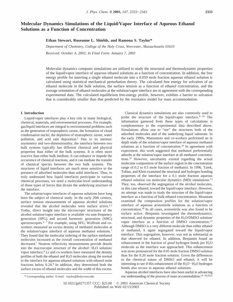
(b) Ethanol Orientations.Figure 4 shows the orientationaldistributions for the ethanol molecules adsorbed at the solution/

Figure 3. Density profiles of the four aqueous ethanol solutions at 298 K. Panels A-D correspond toøethanol ) 0.026, 0.059, 0.11, and 0.40solutions, respectively. The open circles represent the density profiles of the H2O molecules and the solid circles represent the density profiles ofthe ethanol molecules. The solid lines are the fits of the H2O data obtained with the hyperbolic tangent function given in eq 5. With the exceptionof panel D, the dashed lines are the fits to the ethanol data obtained with the Gaussian function given in eq 6 assuming a constant density of ethanolin the bulk of the solution. The ethanol distribution shown in panel D is fit with eq 5 (dashed line).

TABLE 4: Results of Fitting the z-Dependent DensityProfiles of the Ethanol Molecules with the GaussianFunction Given in Eq 6a

øethanol zfilmb (Å) σe(Å) Γethanol(mol/cm2) ((0.5)

0.026 (17.9 4.3 ((0.2) 2.0× 10-10

0.059 (16.8 4.8 ((0.3) 3.4× 10-10

0.11 (16.2 4.9 ((0.5) 4.6× 10-10

0.40c (25.5 4.4 ((0.2) 5.1× 10-10

a In all cases, the temperature is maintained at 298 K. Also shownis the calculated surface excess,Γethanol. b The( sign indicates that thesimulation cell is centered at zero and that an excess of ethanol is foundat each of the two interfaces: one at+zfilm and one at-zfilm. c Theethanol distribution for theøethanol ) 0.40 solution is not Gaussian inshape. It instead has the same shape as the water density distributions.Thus, its film position,zfilm, and film thickness,σe, were calculatedusing the hyperbolic tangent function given in eq 5 and not the Gaussianfunction given in eq 6.

Fe(z) ) Fe0 exp[ - 4(ln 2)(z - zfilm)2

σe2 ] (6)

Γethanol)Nethanol- FbulkV

S(7)

MD of Liquid/Vapor Interface of Ethanol Solutions J. Phys. Chem. B, Vol. 107, No. 10, 20032337

vapor interface. In addition to the four aqueous solutions,orientational data is also provided for pure ethanol. The anglemonitored is that between the surface normal and the C-O bondaxis of ethanol. This angle can vary from 0° to 180° with anangle of 90° corresponding to the bond lying parallel to theplane of the surface. All five curves have been independentlypeak-normalized. In all cases, the hydrophilic end of the ethanolmolecule points into the solution lamella, as indicated by theangle between the surface normal and the C-O bonds beingpeaked aboutθ equal to 180°. The C-O peak distribution isbroader for the higher concentration and pure ethanol solutions(the open symbols in Figure 4) than for the lower concentrationethanol solutions (the closed symbols in Figure 4). This changein the width of the orientational distribution occurs becausefewer molecules are competing for the finite number of surfacesites in the lower concentrations. Thus, the individual ethanolmolecules can minimize the interaction of their hydrophobiccarbon chain with the underlying water molecules. At the higherethanol concentrations, a competition exists between minimizingthe interactions of the carbon chains with the underlying H2Omolecules and packing as many ethanol molecules on the surfaceas possible. An increased ordering as a function of decreasedbulk concentration was also reported in the experimental SFGmeasurements of aqueous methanol solutions.7

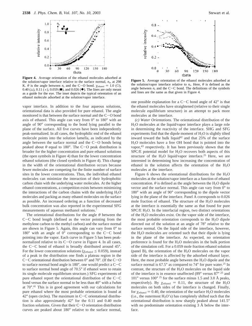
The orientational distributions for the angleθ between theC-C bond length (defined as the vector pointing from themethylene carbon to the methyl carbon) and the surface normalare shown in Figure 5. Again, this angle can vary from 0° to180° with an angle of 0° corresponding to the C-C bondpointing into the vapor. Each curve in Figure 5 has been peak-normalized relative to its C-O curve in Figure 4. In all cases,the C-C bond of ethanol is broadly distributed around 45°.For the lower concentration solutions (øethanole 0.059), insteadof a peak in the distribution one finds a plateau region in theC-C orientational distribution between 0° and 70°. (If the C-Oto surface normal bond angle is 180°, one would predict a C-Cto surface normal bond angle of 70.5° if ethanol were to retainits single molecule equilibrium structure.) SFG experiments ofpure ethanol report the orientational distribution of the C-Cbond versus the surface normal to be less than 40° with a fwhmat 70°.41 This is in good agreement with our calculations forpure ethanol where the most probable orientation is found at42° (open circles). The maximum in C-C orientational distribu-tion is also approximately 42° for the 0.11 and 0.40 molefraction solutions. Given that their C-O orientation distributioncurves are peaked about 180° relative to the surface normal,

one possible explanation for a C-C bond angle of 42° is thatthe ethanol molecules have straightened (relative to their singlemolecule equilibrium structure) in an attempt to pack moremolecules at the interface.

(c) Water Orientations.The orientational distribution of theH2O molecules at the liquid/vapor interface plays a large rolein determining the reactivity of the interface. SHG and SFGexperiments find that the dipole moment of H2O is slightly tiltedinward toward the bulk liquid42 and that 25% of the surfaceH2O molecules have a free OH bond that is pointed into thevapor,43 respectively. It has been previously shown that theSPC/E potential model for H2O recovers both aspects of thisstructure of the H2O liquid/vapor interface.25 Here, we areinterested in determining how increasing the concentration ofethanol in the solution affects the orientation of the H2Omolecules at the interface.

Figure 6 shows the orientational distributions for the H2Omolecules at the solution/vapor interface as a function of ethanolconcentration.θ is defined as the angle between the H2O dipolevector and the surface normal. This angle can vary from 0° to180° with an angle of 90° corresponding to the dipole vectorlying in the plane of the interface. Panel A corresponds to 0.026mole fraction of ethanol. The structure of the H2O moleculesat the interface is essentially the same as that found for pureSPC/E H2O. In the interfacial region, two distinct orientationsof the H2O molecules exist. On the vapor side of the interface,the most probable orientation corresponds to the H2O dipoledirected out of the solution at an angle of 78° relative to thesurface normal. On the liquid side of the interface, however,the H2O molecules are oriented such that their dipole is lyingin the plane of the interface. As expected, no orientationpreference is found for the H2O molecules in the bulk portionof the simulation cell. For a 0.059 mole fraction ethanol solution(panel B), the orientation of the H2O molecules on the vaporside of the interface is affected by the adsorbed ethanol layer.Here, the most probable angle between the H2O dipole and thesurface normal is 67.5° as compared to 74° for pure water.25 Incontrast, the structure of the H2O molecules on the liquid sideof the interface is in essence unaffected (89° versus 87° 25 and101° versus 100° 25 for the surface minus 1.5 and 3.0 Å peaks,respectively). Byøethanol ) 0.11, the structure of the H2Omolecules on both sides of the interface is changed. Finally,for øethanol) 0.40, the orientation of the surface H2O molecules(i.e., the outermost H2O’s) has completely shifted such that theorientational distribution is now sharply peaked about 141.5°with no predominate orientation existing 3 Å below the inter-face.

Figure 4. Average orientation of the ethanol molecules adsorbed atthe solution/vapor interface relative to the surface normal,nz, at 298K. θ is the angle betweennz and the C-O bond.øethanol ) 1.0 (O),0.40 (4), 0.11 (×), 0.059 (b), and 0.026 ([). The lines are only meantas a guide for the eye. The inset depicts the typical orientation of anethanol molecule adsorbed at the solution/vapor interface.

Figure 5. Average orientation of the ethanol molecules adsorbed atthe solution/vapor interface relative tonz. Here,θ is defined as theangle betweennz and the C-C bond. The definitions of the symbolsand lines are the same as that given in Figure 4.

2338 J. Phys. Chem. B, Vol. 107, No. 10, 2003 Stewart et al.

As the concentration of ethanol is increased, the orientationof the vapor-side H2O molecules at first shifts to a smaller angleversus the surface normal and then rapidly shifts toward largerangles. As the ethanol concentration is increased from 0.026 to0.059 mole fraction, the distribution of the H2O molecules hasbroadened and shifted to a smaller angle relative to the surfacenormal. This shift allows more ethanol molecules to adsorb in

the finite number of available surface sites but yet maintainsthe highly structured nature of the H2O surface. However, asthe concentration of ethanol molecules increases beyondøethanol

) 0.059, the highly ordered H2O structure is abandoned inchoice of adsorbing more ethanol molecules at the interface.By øethanol ) 0.40, the H2O structure has completely changedto one in which the dipole moments of the H2O molecule are

Figure 6. Average orientational distribution of the H2O dipole vector relative to the surface normal,nz, as a function of concentration: (solidcurve) orientation of the H2O molecules in the bulk of the solution; (b) orientation of the H2O molecules 3 Å from the surface; (×) orientation ofthe H2O molecules 1.5 Å from the surface; (O) orientation distribution of the H2O molecules at the surface. Panels A-D correspond toøethanol)0.026, 0.059, 0.11, and 0.40, respectively. The lines are a smooth fit to the data.

Figure 7. Orientation distribution of H2O’s OH bond relative to the surface normal as a function of concentration. The definitions of the varioussymbols and panels are the same as that given in Figure 6.

MD of Liquid/Vapor Interface of Ethanol Solutions J. Phys. Chem. B, Vol. 107, No. 10, 20032339

pointing into the bulk liquid. This allows both the oxygen atomand perhaps one of the hydrogen atoms on the H2O moleculesto hydrogen bond with the adsorbed ethanol molecules.

Figure 7 gives another view of the orientational distributionof the H2O molecules at the solution/vapor interface. Here,φ

is defined as the angle between the O-H vector and the surfacenormal. Again, atøethanol) 0.026, the surface structure is verysimilar to that of pure H2O whereφ is peaked at 0° and 120°for the outermost surface H2O’s.25 As the ethanol concentrationapproaches 0.40 mole fraction, this structure changes to onewhere the distribution ofφ is sharply peaked at 180° versusthe surface normal. Having the O-H bonds point 180° into thebulk, places the oxygen atoms in perfect position to hydrogenbond with the surface layer of ethanol molecules.

(d) Hydrogen Bonding.Below we have analyzed the effectof concentration on the H2O-H2O, ethanol-ethanol, and H2O-ethanol hydrogen bonding structure. For DMSO-H2O solutions,Benjamin found that the number of H2O-H2O hydrogen bondsmonotonically decreased as the Gibb’s surface was ap-proached.12 The degree of this decrease seemed to be indepen-dent of concentration. However, when he looked at the numberof hydrogen bonds per H2O molecule divided by the H2O-H2O coordination number, i.e., the fraction ofgoodhydrogenbonds, Benjamin found that the degree of hydrogen bondingwas affected more by the presence of the surface at lowerDMSO concentrations than at higher DMSO concentrations.12

Figure 8 shows a similar analysis of the H2O-H2O hydrogenbonding as a function of concentration for ethanol/H2O solutions.In this analysis, we consider two molecules to be hydrogen-bonded if their O-O separation is less than 3.5 Å, their H-Oseparation is less than 2.6 Å, and their H-OH bond angle isgreater than 140°. It has been demonstrated that the hydrogenbonding information obtained from this type of structuraldefinition is similar to that obtained using a definition basedupon the pair interaction energy.12,13

The top panel of Figure 8 shows the total number of H2O-H2O hydrogen bonds per H2O molecules as a function ofposition along thezdirection for the four solutions. The numberof H2O-H2O hydrogen bonds in the bulk region of the solutionis inversely proportional to the ethanol concentration anddecreases monotonically as the solution/vapor interface isapproached. The lines are a fit of this monotonic decrease withthe hyperbolic tangent function given in eq 5 whereFV andFL

are now defined as the number of hydrogen bonds per H2Omolecule in the vapor phase and liquid phase, respectively.Although the fit of eq 5 to the hydrogen bonding data is not asgood as its fit to the density data, it provides a qualitative pictureof how the presence of the ethanol molecules affect the hydrogenbonding structure of the interfacial H2O molecules. Within theerrors of the fits, no concentration dependence is found for thedistance over which the number of hydrogen bonds per H2Omolecule decays from 90% to 10% of its bulk value. (From thefits, distances of 9.8, 9.4, 9.9, and 10.3 Å are found for the0.026, 0.059, 0.11, and 0.44 ethanol mole fraction solutions,respectively.)

The bottom panel in Figure 8 shows the fraction ofgoodhydrogen bonds. This value is obtained by dividing the numberof hydrogen bonds per H2O molecule by the average coordina-tion number of H2O at a given depth. As in the DMSO work ofBenjamin,12 the probability of finding agood H2O-H2Ohydrogen bond increases as the concentration of ethanolincreases. In the case oføethanol) 0.026 solution, approximately88% of the bulk H2O-H2O nearest-neighbor interactions arevia hydrogen bonding. This number increases to 94% for the

øethanol) 0.40 solution. However, the effect of the interface isnot as clear as that seen in the DMSO work. For all foursolutions, the fraction of good hydrogen bonds does increaseas the H2O molecules approach the surface. However, quanti-tatively, this fraction ofgood hydrogen bonds differs as afunction of concentration. For the low concentrations (øethanol

e 0.059), 93% of the H2O-H2O nearest neighbor interactionsat the interface are via hydrogen bonding; whereas, at the higherconcentrations (øethanole 0.11), 98% of the H2O-H2O nearestneighbor interactions are via hydrogen bonding. Thus, the effectof the interface is less exact.

Figure 9 shows the number of ethanol-ethanol hydrogen bondsper ethanol molecule as a function of concentration. Here, wedefine two ethanol molecules to be hydrogen-bonded if the O-Oseparation is less than 3.5 Å, the O-H separation is less than2.5 Å, and the H-OH bond angle is less than 140° (where His the alcohol not the alkyl hydrogen of ethanol). This definitionis similar to that used by Gao and Jorgensen in their examinationof hexanol-hexanol hydrogen bonding at aqueous interfaces.44

As the interface is approached an enhancement in the numberof ethanol-ethanol hydrogen bonds is found. These numbers,however, are quite small with the maximum number approach-ing one ethanol-ethanol hydrogen bond for the 0.40 ethanol molefraction solution. The orientation of the ethanol molecules at

Figure 8. Top panel: number of H2O-H2O hydrogen bonds per H2Omolecule as a function ofz position for the four aqueous ethanolsolutions: øethanol) 0.40 (O), 0.11 (×), 0.059 (b), and 0.026 ([). Thelines are a fit to the hyperbolic tangent function given in eq 5. Bottompanel: number of H2O-H2O hydrogen bonds per H2O molecule dividedby the z-dependent coordination number of H2O. The dotted, shortdashed, long dashed, and solid lines correspond toøethanol) 0.40, 0.11,0.058, and 0.026 solution, respectively. These lines are a smooth fit tothe data.

2340 J. Phys. Chem. B, Vol. 107, No. 10, 2003 Stewart et al.

the interface precludes more ethanol-ethanol hydrogen bondsfrom occurring.

The average number of ethanol-H2O hydrogen bonds perethanol molecule as a function of distance from the interface isgiven in Figure 10. The same structural definition for a hydrogenbond as that given above is employed here. (Molecules withOwater-Halcohol and Oalcohol-Hwater separations less than 2.6 Åare further considered as possibly being hydrogen-bonded.) Wesee a monotonic decrease in ethanol-H2O hydrogen bonds asthe interface is approached. This decrease is more pronouncedfor the lower ethanol concentrations than for the higher ethanolconcentrations. If the information in Figures 9 and 10 is takentogether, the total number of hydrogen bonds per ethanolmolecule remains fairly constant for theøethanol) 0.40 solutionbut decreases from 2.2 hydrogen bonds per ethanol in the bulkto approximately 1.5 hydrogen bonds per ethanol at the interfacefor the øethanol) 0.059 solution.

As with the H2O-H2O hydrogen bonding data, we have fitthe ethanol-H2O hydrogen bond profiles with the hyperbolictangent function given in eq 5. Although the individual fits toeq 5 are not good as the number of hydrogen bonds approacheszero, the errors systematically overestimate the thickness of theinterface. Thus, these fits provide a qualitative picture of howthe ethanol-H2O hydrogen bond profile is affected by thesolution/vapor interface as a function of concentration. Figure

11 shows the same data as that shown in Figure 10 but dividesit into the number of ethanol-H2O hydrogen bonds per ethanolwhere ethanol is the hydrogen acceptor (top panel) and thenumber of H2O-ethanol hydrogen bonds per ethanol whereethanol is the hydrogen donor (bottom panel). The interfacethicknesses obtain from the fits of these data to eq 5 are givenin Table 5. Again these thicknesses are only qualitatively correct.We quickly see, however, that forøethanole 0.11 the ethanol-H2O hydrogen bonding structure decays from 90% to 10% ofits bulk value over a longer distance when the ethanol moleculeis the hydrogen donor than when the ethanol molecule is thehydrogen acceptor. Because a distinct orientation exists for theethanol molecules at the interface, for an ethanol to be thehydrogen donor, the surface H2O molecules would need to orientthemselves with their dipole vector pointing into the bulksolution. This is in direct contrast to what is found in pure H2O.

Figure 9. Number of ethanol-ethanol hydrogen bonds per ethanolmolecule as a function ofz position. The definitions of various linestypes are same as that given for the bottom panel of Figure 8.

Figure 10. Distribution of ethanol-H2O hydrogen bonds per ethanolmolecule. These data contain those hydrogen bonds where ethanol isacting both as a hydrogen acceptor and donor.øethanol) 0.40 (O), 0.11(×), 0.059 (b), and 0.026 ([). The lines are a fit to the hyperbolictangent function given in eq 5.

Figure 11. Distribution of ethanol-H2O hydrogen bonds per ethanolmolecule. The top panel corresponds to those ethanol-H2O hydrogenbonds where ethanol is acting as the hydrogen acceptor and the bottompanel corresponds to those ethanol-H2O hydrogen bonds where ethanolis acting as the hydrogen donor. The line styles are defined in Figure10 and are a fit of the data to the hyperbolic tangent function given ineq 5.

TABLE 5: Distance Over Which the Number ofEthanol-H2O Hydrogen Bonds Per Ethanol MoleculeDecays from 90% of Its Bulk Value to 10% of Its BulkValuea

ethanol-H2O hydrogen bonding ‘10-90’ distance

øethanol ethanol as H acceptor (Å) ethanol as H donor (Å)

0.026 9.6 5.50.059 11.7 5.90.11 12.9 7.80.40 12.5 15.9

a These distances were determined by fitting the ethanol-H2Ohydrogen bonding profiles with eq 5.

MD of Liquid/Vapor Interface of Ethanol Solutions J. Phys. Chem. B, Vol. 107, No. 10, 20032341

Thus, the likelihood of finding an ethanol-H2O configurationof this sort at the interface is not high and the number of thesetypes of ethanol-H2O hydrogen bonds quickly falls to zero.On the other hand, the orientation of the interfacial ethanolmolecules does not adversely affect the possibility of formingan ethanol-hydrogen-acceptor ethanol-H2O hydrogen bond.Hence, at low concentrations, the idea that H2O moleculesmaintain their strong hydrogen bonding network at the expenseof forming more ethanol-H2O interactions is reinforced. Forøethanol) 0.40, ethanol’s hydrogen donor curve (bottom panel)decays from 90% to 10% of the bulk value over a longerdistance than its hydrogen acceptor curve (top panel). Here,packing more ethanol molecules at the interface becomes thegoverning force for determining the interfacial structure.

C. Potential of Mean Force.The free energy profile for theinsertion of a single ethanol molecule into aøethanol ) 0.059ethanol/H2O solution has been calculated using the thermody-namic perturbation approach, and is shown in the top panel ofFigure 12. The portion of the ethanol and H2O density profilesthrough which the molecule is inserted is shown in the lowerpanel of Figure 12. This density profile corresponds to that givenin Figure 3B but shows only half of the range ofz. The reactioncoordinate is chosen to be the distance between the centers ofmass of the impinging ethanol molecule and of the bulk solution,such that this coordinate is perpendicular to the solution/vaporinterface. The zero of energy is defined to be when theimpinging ethanol molecule is far (>10 Å) from the solutioninterface. The free energy for solvation,∆Gsolv, is a measurementof the free-energy difference between a molecule being solvatedin the bulk of the solution versus the molecule being in the gasphase. Thus,∆Gsolv can be measured directly from Figure 12to have a value of-5.2 kcal/mol. The experimental value for∆Gsolv for an ethanol molecule in pure H2O is-5.0 kcal/mol.45,46

This is very good agreement. As shown in the density profile

for øethanol) 0.059 (bottom panel of Figure 12), the density ofethanol in the bulk of the solution is quite low (<0.1 g/cm3),thus little difference should exist between∆Gsolv for an ethanolmolecule in pure H2O and∆Gsolv for an ethanol molecule in a0.059 mole fraction aqueous ethanol solution. Therefore, wefeel confident that the potentials that we are employing providea quantitative description of the energetics of the ethanol-H2Osystem.

As described earlier in the discussion of surface excess,ethanol is surface active and thus preferentially binds at thesolution/vapor interface. This is confirmed by the broadminimum in the free energy profile between 13 and 18 Å. (TheGibb’s interface for the bulk solution and the peak in the ethanoldensity are located at 15.86 and 16.8 Å, respectively.) The freeenergy for adsorption,∆Gads, which is the calculated energydifference for an ethanol molecule being located in thisinterfacial minimum relative to the gas phase, is-6.1 kcal/mol. Thus, a+0.9 kcal/mol barrier exists between the surfacesite and the bulk solvation site (the difference between∆Gads

and∆Gsolv). No additional activation barrier, however, is foundfor the insertion of an ethanol molecule into a bulkøethanol )0.059 aqueous ethanol solution. The lack of a large barrierbetween the surface site and the bulk solvated site is inagreement with our previous calculations for the insertion of asingle ethanol molecule into bulk H2O15,16 but is in definitedisagreement with the ideas of the resistance model.20,21

Within the resistance model, the mass-accommodation coef-ficient, R, for the insertion of an ethanol molecule into the bulkof a solution can be calculated via21

where∆Gdesorbis equal to-∆Gadsorb, ∆Gsolv‡ is equal to (∆Gsolv

- ∆Gadsorb) when no activation barrier is present,T is thetemperature in Kelvin, andR is the gas constant. Given ourvalues for ∆Gadsorb and ∆Gsolv, the mass accommodationcoefficient for inserting an ethanol molecule into a 0.059 molefraction ethanol solution is 1.0 at 298 K. The experimental valuefor the mass accommodation coefficient for inserting an ethanolmolecule into a dilute ethanol/H2O droplet is 0.0093 at 298 K.20

Previously, we hypothesized that the difference between theexperimental value ofR and that calculated in our simulationsmight be due to the fact that the experimental model onlyallowed the impinging ethanol molecule to interact with acleanH2O surface.15 However, given the surface activity of ethanolin aqueous solutions, real ethanol/H2O solutions have afilm ofethanol on them through which the impinging ethanol moleculewould need to traverse before becoming solvated in the bulksolution. Our current findings suggest that the existence of sucha film is not the difference between the experiments andsimulations and that a more fundamental difference existsbetween the mass accommodation coefficients being measuredin the experiments and those being calculated via the MDsimulations within the resistance model. What this fundamentaldifference is deserves further exploration.

IV. Summary and Conclusions

Molecular dynamics computer simulations have been usedto explore both the structure of the liquid/vapor interface ofethanol/H2O solutions as a function of concentration and tocalculate the mass accommodation coefficient for the insertion

Figure 12. Top panel: free energy profile for the insertion of a singleethanol molecule into aøethanol) 0.059 mole fraction aqueous ethanolsolution at 298 K. Bottom panel: corresponding region of the densityprofile for theøethanol) 0.059 ethanol solution through which the ethanolmolecule is inserted. The open circles correspond to the H2O densityprofile and the closed circles correspond to the ethanol density profile.

R1 - R

)exp(-

∆Gsolv‡

RT )exp(-

∆Gdesorb

RT )(8)

2342 J. Phys. Chem. B, Vol. 107, No. 10, 2003 Stewart et al.

of an ethanol molecule into aøethanol) 0.059 aqueous ethanolsolution. Using a combination of the SPC/E H2O potential23

and the OPLS/AA ethanol potential,26 we have been able toreproduce the experimental surface tension results as a functionof concentration. In addition, the calculated free energy forsolvation in the bulk liquid and the average orientation of ethanolmolecules at the solution/vapor interface agree well with thecorresponding experimental data. Thus, we believe that thiscombination of potential functions adequately describes theaqueous ethanol solution/vapor interface. At all concentrations,ethanol is found to be surface active. Ethanol molecules sit atthe surface with their hydrophobic alkyl tails pointing into thevapor and their hydrophilic alcohol groups pointing into thesolution. Belowøethanol ) 0.11, the orientation of the surfaceH2O molecules seems to be unaffected by the presence of thesurface ethanol molecules. However, aboveøethanol) 0.11, thestructure of the underlying H2O molecules is greatly changed.This may have measurable affects on the surface reactivity andsolvation properties of these interfaces.

Below øethanol) 0.11, the distance over which the number ofethanol-H2O hydrogen bonds decays from 90% to 10% of thebulk number is longer for those hydrogen bonds where ethanolis the hydrogen acceptor as compared to when ethanol is thehydrogen donor. The opposite effect is seen for the 0.40 ethanolmole fraction solution. Together with the ethanol and H2Oorientation data, this seems to support the idea that at lowethanol concentrations maintaining the strong H2O-H2O hy-drogen bonding network is the governing force in determiningthe interfacial structure. While at higher ethanol concentrations,where the orientation of the surface H2O molecules is oppositeto that found in pure H2O, the need to pack more ethanolmolecules at the hydrophobic liquid/vapor interface becomesthe dominant force.

Finally, the mass accommodation coefficient calculated forthe insertion of a single ethanol molecule through the ethanolexcess and into the bulk of an aqueous ethanol solution remainsin disagreement with the experimental measurements of the massaccommodation coefficient.

Acknowledgment. We thank Drs. Liem X. Dang, GregoryK. Schenter, Bruce C. Garrett, and Ilan Benjamin for insightfuldiscussions. We also thank the following organizations for theirsupport of this work: Dreyfus Foundation (Grant # SU-97-048),the Research Corp. (Grant # CC5158), and the AmericanChemical Society, Petroleum Research Fund (ACS-PRF Grant# 36806-GB6).

References and Notes

(1) Schwarzenbach, R. P.; Gschwend, P. M.; Imboden, D. M.EnVi-ronmental Organic Chemistry; John Wiley & Sons: New York, 1993; pp56-254.

(2) MacRitchie, F.Chemistry at Interfaces; Academic Press: NewYork, 1990; pp 12-23, 32-38.

(3) Schofield, R. K.; Rideal, E. K.Proc. R. Soc. London1925, A109,60.

(4) Eisenthal, K. B.Chem. ReV. 1996, 96, 1343.(5) Gragson, D. E.; Richmond, G. L.J. Phys. Chem. B1998, 102,

3847.(6) Miranda, P. B.; Shen, Y. R.J. Phys. Chem. B1999, 103, 3292.(7) Wolfrum, K.; Graener, H.; Laubereau, A.Chem. Phys. Lett.1993,

213, 41.(8) Li, Z. X.; Lu, J. R.; Styrkas, D. A.; Thomas, R. K.; Rennie, A. R.;

Penfold, J. Mol. Phys.1993, 80, 925.(9) Matsumoto, M.; Kataoka, Y.J. Chem. Phys.1989, 90, 2398.

(10) Matsumoto, M.; Takaoka, Y.; Kataoka, Y.J. Chem. Phys.1993,98, 1464.

(11) Benjamin, I.Chem. ReV. 1996, 96, 1449.(12) Benjamin, I.J. Chem. Phys.1999, 110, 8070.(13) Tarek, M.; Tobias, D. J.; Klein, M. L.J. Chem. Soc., Faraday Trans.

1996, 92, 559.(14) Taylor, R. S.; Ray, D.; Garrett, B. C.J. Phys. Chem. B1997, 101,

5473.(15) Taylor, R. S.; Garrett, B. C.J. Phys. Chem. B1999, 103, 844.(16) Wilson, M. A.; Pohorille, A.J. Phys. Chem. B1997, 101, 3130.(17) Somasundaram, T.; Lynden-Bell, R. M.; Patterson, C. H.Phys.

Chem. Chem. Phys.1999, 1, 143.(18) Mountain, R. D.J. Phys. Chem. B2001, 105, 6556.(19) Dang, L. X.; Chang, T.-M.J. Phys. Chem. B.2002, 106, 235.(20) Jayne, J. T.; Duan, S. X.; Davidovits, P.; Worsnop, D. R.; Zahniser,

M. S.; Kolb, C. E.J. Phys. Chem.1991, 95, 6329.(21) Nathanson, G. M.; Davidovits, P.; Worsnop, D. R.; Kolb, C. E.J.

Phys. Chem.1996, 100, 13007.(22) Donaldson, D. J.; Anderson, D.J. Phys. Chem. A1999, 103, 871.(23) Berendsen, H. J. C.; Gigera, J. R.; Straatsma, T. P.J. Phys. Chem.

1987, 91, 6269.(24) Alejandre, J.; Tildesley, D. J.; Chapela, G. A.J. Chem. Phys.1995,

102, 4574.(25) Taylor, R. S.; Dang, L. X.; Garrett, B. C.J. Phys. Chem.1996,

100, 11720.(26) Jorgensen, W. L.; Maxwell, D. S.; Tirado-Rives, J.J. Am. Chem.

Soc.1996, 118, 11225.(27) Allen, M. P.; Tildesley, D. J.Computer Simulations of Liquids;

Oxford University Press: New York, 1987.(28) Pearlman, D. A.; Case, D. A.; Caldwell, J. C.; Seibel, G. L.; Singh,

U. C.; Weiner, P.; Kollman, P.AMBER, 4.0 ed.; University of California:San Francisco, CA 1991.

(29) Verlet, L.Phys. ReV. 1967, 159, 98.(30) Berendsen, H. J. C.; Postama, J. P. M.; van Gunsteren, W. F.;

DiNola, A.; Haak, J. R.J. Chem. Phys.1980, 72, 2384.(31) Ryckaert, J.-P.; Ciccotti, G.; Berendsen, H. J. C.J. Comput. Phys.

1977, 23, 327.(32) Kirkwood, J. G.J. Chem. Phys.1930, 3, 300.(33) Zwanzig, R. W.Chem. Phys.1954, 22, 1420.(34) Huston, S. E.; Rossky, P. J.; Aichi, D. A.J. Am. Chem. Soc.1989,

111, 5680.(35) Smith, D. E.; Dang, L. X.J. Chem. Phys.1994, 100, 3757.(36) Fowler, R. H.Proc. R. Soc.1937, A159, 229.(37) Kirkwood, J. G.; Buff, F. P.J. Chem. Phys.1949, 17, 338.(38) Salomons, E.; Mareschal, M.J. Phys.: Condens. Matter1991, 3,

3645.(39) Taylor, R. S. Manuscript in preparation.(40) Townsend, R. M.; Rice, S. A.J. Chem. Phys.1985, 82, 4391.(41) Stanners, C. D.; Du, Q.; Chen, R. P.; Cremer, P.; Somorjai, G. A.;

Shen, Y. R.Chem. Phys. Lett.1995, 232, 407.(42) Goh, M. C.; Hicks, J. M.; Kemnitz, K.; Pinto, G. R.; Bhattacharyya,

K.; Eisenthal, K. B.; Heinz, T. F.J. Phys. Chem.1988, 92, 5074.(43) Du, Q.; Freysz, E.; Shen, Y. R.Science1994, 264, 826.(44) Gao, J.; Jorgensen, W. L.J. Phys. Chem.1988, 92, 5813.(45) Cabani, S.; Gianni, P.; Mollica, V.; Lepori, L.J. Solution Chem.

1981, 10, 563.(46) Ben-Naim, A.; Marcus, Y.J. Chem. Phys. 1984, 81, 2016.

MD of Liquid/Vapor Interface of Ethanol Solutions J. Phys. Chem. B, Vol. 107, No. 10, 20032343