Molecular BioSystems b707506e - dbkgroup.orgdbkgroup.org/Papers/wilkinson_mbs_ppt08.pdf ·...

Molecular BioSystems b707506e

PAPER

1

Proximate parameter tuning for biochemical networkswith uncertain kinetic parameters

Stephen J. Wilkinson, Neil Benson and Douglas B. Kell

Parameter estimation is a hard, important and usuallyunderdetermined problem. We introduce the constraint thatthe estimated parameters should be as close as possible tostated values in a way that is both deterministic and veryeffective.

Please check this proof carefully. Our staff will not read it in detail after you have returned it.

Translation errors between word-processor files and typesetting systems can occur so the whole proof needs to be read.

Please pay particular attention to: tabulated material; equations; numerical data; figures and graphics; and references. If

you have not already indicated the corresponding author(s) please mark their name(s) with an asterisk. Please e-mail a list of

corrections or the PDF with electronic notes attached — do not change the text within the PDF file or send a revised

manuscript.

Please bear in mind that minor layout improvements, e.g. in line breaking, table widths and graphic placement, are routinely

applied to the final version.

We will publish articles on the web as soon as possible after receiving your corrections; no late corrections will be made.

Please return your final corrections, where possible within 48 hours of receipt, by e-mail to: [email protected]

Electronic (PDF) reprints will be provided free of charge to the corresponding author. Enquiries about purchasing paper

reprints should be addressed via: http://www.rsc.org/Publishing/ReSourCe/PaperReprints/. Costs for reprints are below:

Reprint costs

No of pages Cost for 50 copies Cost for each additional 50 copies

2–4 £180 £115

5–8 £300 £230

9–20 £600 £480

21–40 £1100 £870

.40 £1700 £1455

Cost for including cover of journal issue:

£50 per 50 copies

Proximate parameter tuning for biochemical networks with uncertain; kinetic parameters< {

Stephen J. Wilkinson,ab Neil Bensonc and Douglas B. Kell*ab

Received 18th May 2007, Accepted 26th July 2007

First published as an Advance Article on the web

DOI: 10.1039/b707506e

It is commonly the case in biochemical modelling that we have knowledge of the qualitative

‘structure’ of a model and some measurements of the time series of the variables of interest

(concentrations and fluxes), but little or no knowledge of the model’s parameters. This is, then, a

system identification problem, that is commonly addressed by running a model with estimated

parameters and assessing how far the model’s behaviour is from the ‘target’ behaviour of the

variables, and adjusting parameters iteratively until a good fit is achieved. The issue is that most

of these problems are grossly underdetermined, such that many combinations of parameters can

be used to fit a given set of variables. We introduce the constraint that the estimated parameters

should be within given bounds and as close as possible to stated nominal values. This

deterministic ‘proximate parameter tuning’ algorithm turns out to be exceptionally effective, and

we illustrate its utility for models of p38 signalling, of yeast glycolysis and for a benchmark

dataset describing the thermal isomerisation of a-pinene.

Introduction

Various types of computational modelling are being used both

to understand biochemical systems and to make sense of

existing (often omics) data, especially as part of iterative

experimental design programmes aimed at the serial genera-

tion of new data and hypotheses.1–9

We consider initially the problem of tuning a detailed kinetic

model of a signalling pathway whose stoichiometric structure

is known but in which most of the parameter values have not

been experimentally determined and are therefore highly

uncertain. We assume that very limited time course data of a

few (perhaps only one) participatory species are available. We

would like to ‘fit’ our model to the available data. In this

context, traditional parameter estimation techniques10–12 are

of limited utility13 given the large number of undetermined

model parameters and the relatively few measured variables.

Put another way, the models are typically grossly under-

determined and many combinations of parameters can fit the

measured variables.

The above problem is a very common one for biochemical

and other models, and a common remedy is to use a greatly

reduced model in which the number of unknown parameters

does not swamp the number of measured variables.14–17 This

approach can provide valuable insights but model reduction

techniques often make big structural simplifications to the

original kinetic scheme, thereby discarding the considerable

biological knowledge that went into building them in the first

place. In this paper, therefore, we adopt an alternative appro-

ach in which we retain the detailed kinetic structure of the

model. We navigate the uncertain parameter space using local

sensitivity information in order to match the model with

measured output features. In such an under-defined system

there may well be many distinct parameter combinations that

fit the measured data but we seek those that are closest to the

nominal parameter values rather than those at the extremes of

the parameter space. This turns out to be an extremely

effective method.

One can separate the information required to construct a

detailed ‘forward’ kinetic model of a signalling network into

two types: structural data and kinetic data. Structural data

describe the nodes and links of the signalling network, i.e. the

species, reactions and the stoichiometric quantities of each

species consumed and produced by each reaction together with

effector interactions. Kinetic data consist of the functional

form of the rate equation for each reaction and the values of

the associated kinetic parameters. For many well-studied

signalling networks the structural data are known with a com-

paratively high level of confidence but the kinetic parameters

are known with far less certainty. The proximate tuning

method presented in this paper can use very limited output

data to find reasonable values for the model parameters.

In the next sections we develop the mathematical framework

before presenting some results.

Background

A typical model of a biochemical network consists of a set of

ordinary differential equations that govern the temporal

evolution of the variable species.

aSchool of Chemistry, Princess St, Manchester, UK M1 7DN.E-mail: [email protected]; [email protected];Fax: +44 (0)161 306 4556; Tel: +44bThe Manchester Centre for Integrative Systems Biology, ManchesterInterdisciplinary Biocentre, The University of Manchester, Princess St,Manchester, M1 7DN, UKcPfizer Central Research, Ramsgate Road, Sandwich, Kent, UKCT13 9NJ. E-mail: [email protected]{ Electronic supplementary information (ESI) available: SBMLmodels. See DOI: 10.1039/b707506e

PAPER www.rsc.org/molecularbiosystems | Molecular BioSystems

This journal is � The Royal Society of Chemistry 2007 Mol. BioSyst., 2007, 3, 1–25 | 1

1

5

10

15

20

25

30

35

40

45

50

55

59

1

5

10

15

20

25

30

35

40

45

50

55

59

dX

dt~f X ,hð Þ (1)

X(t0) = X0 (2)

Here, X represents the vector of n species concentrations and

h is the vector of m parameters:

X = [x1 x2…xi…xn]T (3)

h = [k1 k2…kj…km]T (4)

In general, the rate of change of species concentration

variable xi depends on a non-linear function of the concentra-

tion variables and the model parameters.

Parameter uncertainty is taken into account by assigning

each parameter value a nominal value k0j , a lower bound kmin

j

and an upper bound kmaxj

kminj ƒk0

j ƒkmaxj V j (5)

In the absence of experimental measurements, these values

can be arrived at using biological prior knowledge. The

nominal value corresponds to the most likely value whereas the

bounds are reasonable estimates of the smallest and largest

values that the parameter could take. For such intuitive

estimates the bounds are likely to be rather wide, perhaps

spanning several orders of magnitude. However, the lower

bound for a rate constant is constrained by the known flux

through a pathway if metabolic, and cannot be larger than the

diffusion-controlled limit, for instance. Measured parameters,

on the other hand, will have tighter bounds corresponding to

the experimental error. In the unlikely event of a parameter

value being known exactly, the upper and lower bounds can be

assigned the same value ¡ the noise level, without loss of

generality.

Suppose also that we have some measured concentration

time series that we would like our model to reproduce. We

characterize these time profiles by features (peak value, time to

peak, area under curve etc.) that we can write as a general

function of the concentration profiles and the parameters.

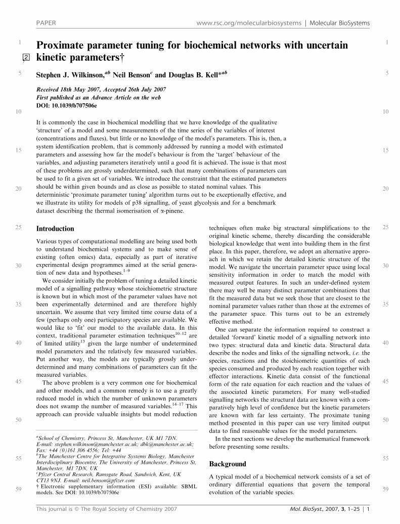
yp~hp hð Þ V p (6)

Here yp is the value of feature simulated by the model for

parameter set h represented by the implicit function hp(h). This

is a sensible strategy since measured data are typically limited

and uncertain such as those illustrated in Fig. 1. It might be the

case that the emphasis is on getting a model output with a peak

value of species A of 0.5 at 60 min. In this case we could use

these two features (i.e. peak value and time to peak, as in

ref. 18,19) to drive the parameter tuning. If on the other hand,

a best fit to the raw time series data is sought, we could define

a separate feature for each measured value at each time point

which the tuning process will seek to match simultaneously.

Examples of both approaches are given later.

In this paper we label the features that we are trying to get

the model to match as ‘target’ features. Whilst these will

usually be measured values, as previously discussed, it may

also be the case that they are simply values that we would

intuitively like the model to emulate (e.g. as in metabolic

engineering11,20–26). Many signalling networks, for example,

have quite well known characteristic response times. Here we

use ‘response time’ in an informal sense meaning the time for

the signalling species of interest to reach peak activation (e.g.

10 min). The modeller would then seek to tune the initial

model to this target value even though it is not (yet) a

measured value.

In general, a model run using the nominal parameter values

will give off-target output features since the parameters have

been estimated without regard either to their measured values

or to those of the output measurements. We would therefore

like to adjust these values so that the simulated target output

feature values of the model are closer to the measured (target)

values. In order to achieve this we propose an iterative scheme

in which the local sensitivity of the required model outputs

with respect to all the parameters is evaluated at each iteration.

This information is then used to predict the smallest step to

take in the parameter space in order to minimize the error

between the model outputs and their target values. The para-

meters are then updated to these new predicted best values and

the ODE model re-run to determine the actual simulated

values of the output features. This iterative loop is then

repeated as the algorithm steps through the parameter space

until the error between the simulated values and the target

values is reduced to a specified tolerance, or stops decreasing,

or the maximum number of iterations is reached. We can list

the key components of the proximate parameter tuning (PPT)

algorithm as follows.

General PPT algorithm

1. Initialise each parameter to its most likely (nominal)

value

2. Run model at current parameter values and compare

outputs to target values

3. If convergence achieved or iteration limit reached then

terminate.

4. Otherwise, calculate sensitivities of model outputs to

each parameter.

5. Use sensitivities to calculate better fitting parameter

values that are proximate to current values and within

minimum/maximum bounds

6. Update current parameters to new values

7. Go to 2.

Fig. 1 Typical time series data for a hypothetical species A.

2 | Mol. BioSyst., 2007, 3, 1–25 This journal is � The Royal Society of Chemistry 2007

1

5

10

15

20

25

30

35

40

45

50

55

59

1

5

10

15

20

25

30

35

40

45

50

55

59

The key steps above are 4. and 5. which can be implemented

in a number of different ways, as briefly discussed below,

to give alternative implementations of the PPT algorithm.

In step 4 we could certainly calculate the first order

sensitivities of the desired model output features with respect

to each parameter. This gives a local linear approximation of

how each varies in the neighbourhood of the current point in

the parameter space. However, for highly non-linear systems,

we may also wish to capture interactions between parameters

via higher order effects. For example, a second order

approximation would be superior to the linear (first order)

approximation, although this improved accuracy would come

at a much greater computational expense. The second order

model would require an estimate of the Hessian matrix

giving the sensitivity of each parameter sensitivity to changes

in that parameter and each of the other parameters in the

model.

Another key consideration in step 4 of the PPT algorithm is

how to calculate the sensitivities. The most general method is

to treat the model equations as a black box and estimate the

sensitivities using small perturbations to the model parameters

and performing a complete simulation after each perturbation.

This has the advantage that it will work for any type of model

and any type of output feature. On the other hand, it may be

possible to calculate sensitivities analytically or using short-cut

methods for certain types of model output without the need to

perform repeated numerical simulations.

Once we have estimated or calculated the sensitivities in

step 4 we also have considerable flexibility as to how we use

them in step 5 to calculate a better set of model parameters.

This is the key part of the PPT algorithm and in general we will

need to solve some sort of optimisation sub-problem in order

to minimize the fitting errors and also stay as close as possible

to the nominal parameter values. In general this will be a

constrained, multi-variable optimisation problem.

For the rest of this paper we use a specific implementation of

the general scheme described above which we call ‘linear

programming-based proximate parameter tuning’ or LP-PPT.

As its name suggests, this implementation involves the solution

of a linear programming (LP) sub-problem27 to calculate

better parameter values (step 5 of the general PPT algorithm

described above). Each sub-problem uses first-order sensiti-

vities and therefore assumes that the contributions of each

parameter to each output feature are linear and independent.

We estimate these sensitivities (step 4) using perturbed simula-

tions of the full model. Despite the assumptions of linearity

implicit in the formulation of each LP sub-problem the method

performs well in the examples discussed below. This is because

of its iterative nature whereby the sensitivity information is

repeatedly updated at each iteration. The steps taken in the

parameter space generally decrease after a handful of iterations

as the algorithm converges on good local solutions.

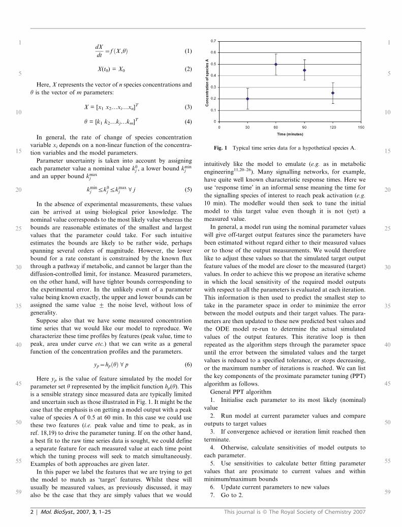
We now provide an illustration of how the LP-PPT

algorithm navigates the uncertain parameter space with the

aim of bringing the model into closer agreement with the target

feature values. In general the parameter space is large since the

upper and lower bounds for each parameter may span several

orders of magnitude. We therefore use variables that describe

the logarithmic (base 10) deviation of each parameter from its

nominal value. Fig. 2 shows how the iterative scheme would

adjust a single parameter in order to match a single target

output feature. For the initial or nominal parameter value

(Iteration 0), the model gives an output feature which is higher

than the target value. In order to find the direction in which to

adjust the parameter, the gradient is calculated (the start of

Iteration 1) and this is used to calculate a new parameter value.

Fig. 2 Hypothetical logarithmic plot of output feature vs. parameter value to illustrate iterative use of local scaled sensitivity to move towards

target value.


1

5

10

15

20

25

30

35

40

45

50

55

59

1

5

10

15

20

25

30

35

40

45

50

55

59

The model is then run at this new parameter value and, if

convergence to the target value has not occurred, the gradient

is calculated at this new parameter value (the start of Iteration

2) and this cycle is repeated until convergence on the target

value is achieved. This process is very similar to Newton’s

method for solving non-linear equations except that in our

case we evaluate the gradients numerically and, in general, we

have multiple targets to meet.

The idea of solving a sequence of linear programming sub-

problems (known as successive linear programming) is also

well a established technique for tackling large-scale non-linear

programming problems arising from engineering applications

in power systems planning and refining scheduling.28,29 It

should also be mentioned that the problem presented in this

paper is a specific instance of a much wider class of ill-posed

inverse problems which have been extensively studied in applied

mathematics. The unique numerical solution of these problems

requires regularization i.e. some additional assumptions con-

straining the decision variables. In this case we penalize the

amount that the parameters deviate from the nominal values

which biases the estimation towards our prior knowledge. There

is a considerable body of work regarding the theoretical

properties of different regularization functions and the choice

of weightings to use30 but detailed discussion of this is beyond

the scope of this paper. The technique has been applied in

biochemical modelling applications in order to reduce the effect

of insensitive parameters during the parameter estimation.31

The linear programming (LP) sub-problem solved at each

iteration r is:

Z~�aa�kkrzX

j

aj Dkzj

rzDk{j

r� �

z�bb�yyrz

X

p

bp Dyzp

rzDy{p

r� � (7)

Minimise:

X

j

Dkzj

r{Dk{j

r� �

{ Dkzj

r{1{Dk{j

r{1� ��

sr{1

p,j ~

c logyg

p

yr{1

p

!z Dyz

pr{Dy{

pr

� �V p

(8)

Subject to:

�kkr§ Dkz

jr{Dk{

jr

� �V j (9)

�kkr§{ Dkz

jr{Dk{

jr

� �V j (10)

�yyr§ Dyz

pr{Dy{

pr

� �V p (11)

�yyr§{ Dyz

pr{Dy{

pr

� �V p (12)

Dkzj

rƒ log

kmaxj

k0j

!V j (13)

Dk{j

rƒ{ log

kminj

k0j

!V j (14)

Note that this is a linear programming problem since it has

an objective function and constraints that are linear with

respect to the decision variables. The logarithmic terms

appearing in some of the equations involve only constant

values for each problem instance and these therefore evaluate

to constant values (right hand sides) for all constraints.

We solve a sequence of sub-problems in which the coeffi-

cients and right hand sides are iteratively varied. The decision

variables for the rth linear programming sub-problem are:

Dkþ9i , Dk{9

i : the positive and negative components of the

logarithm of the fractional deviation of parameter j from its

nominal value after iteration r. So the value of each parameter

j after each iteration r is given by:

krj ~10 Dkz

jr{Dk{

jrð Þ:k0

j V j (15)

Note that we need to include each positive and negative term

explicitly and independently in the LP problem statement. This

is because they have opposite signs in all constraints but have

the same sign in the objective function which seeks to minimize

their sum.

kr: the maximal absolute logarithmic fractional deviation

from the nominal value of all parameters.

Dyþ9n , Dy{9

n : the positive and negative components of the

‘predicted’ logarithmic fractional error of the fitted value

compared to its target value for feature p after iteration r. Note

that the LP sub-problem solves for these quantities exactly but

they are only the predicted actual values. This is because the

LP assumes that parameter sensitivities are locally constant

and have no higher order or interaction terms. Generally this is

not the case and the actual errors between the fitted and target

values after iteration r are calculated by a full simulation of the

original ODE model at the updated parameter values.

yr: the maximal absolute logarithmic fractional error of all

fitted feature values compared to their target values.

The parameters in the linear programming sub-problem (as

opposed to the ODE parameters which are, of course,

variables in the fitting process) are:

ygp: the target value of feature p

k0i , kmin

i , kmaxi : the nominal, minimum and maximum values

for parameter j respectively.

srp;j: the scaled sensitivity of the simulated value (yp) of

feature p with respect to parameter j at iteration r. This value is

calculated numerically by solving the system of ODEs for each

parameter with its value perturbed slightly (0.1%) from the

current value.

a: the penalty associated with the maximal logarithmic frac-

tional deviation of all parameters from their nominal values.

aj: the penalty associated with the logarithmic fractional

deviation of each individual parameter j from its nominal

value.

b: the penalty associated with the maximal logarithmic

fractional error of the fitted value compared to its target value

for all features.

bp: the penalty associated with the logarithmic fractional

error of the fitted value compared to its target value for

feature p.

c: the step length for the feature improvement factor during

each iteration 0 , c , 1.


1

5

10

15

20

25

30

35

40

45

50

55

59

1

5

10

15

20

25

30

35

40

45

50

55

59

In the linear programming formulation summarized above,

the objective function (7) is designed to minimize a linear com-

bination of four terms. The first two terms seek to restrict the

search to proximate points in the parameter space by applying

a penalty to the maximal parameter deviation (first term) and

also including a weighted sum penalizing the individual para-

meter deviations (second term). The third and fourth terms

penalize the error between the simulated and target feature

values. The third term penalizes the maximal error and the

fourth term is a weighted sum of the individual errors which

can be to penalize features differentially depending on the

certainty of their measurement or their perceived importance.

Note the symmetry with which this representation treats the

parameter deviations and the fitting errors. We do not need to

include all the terms but we need one or both of the first two

terms and one or both of the third and fourth terms. In the

examples used in this paper we do not include the second term

(aj~0 V j nor the third term (b = 0). In any case the objective

function defines a trade-off between minimizing the errors and not

straying too far from the nominal parameter values and the

relative values of the penalty coefficients should reflect this.

Usually the former is more important than the latter so we use

bpw�aa V p. For the examples presented in this paper we use:

�aa~1, aj~0 V j, bp~10 V p, �bb~0.

The key constraint is eqn (8) which uses local parameter

sensitivities to adjust the feature values closer to their targets.

This can be seen as a generalization to multiple parameters

of the update formula given in Fig. 2 which was for a single

parameter. The constraint assumes that each parameter

contributes independently and multiplicatively (additively in

the logarithmic space) to each output feature. It ensures that

the optimizer uses first order sensitivity information in order to

adjust the parameters in such a way as to minimize the

predicted penalty at the new point in parameter space. For

multiple features, the optimizer may not be able to match all

the features exactly and therefore seeks the best compromise

parameter adjustment. Note that the actual penalty calculated

at the new point (by direct simulation of the ODEs) is not

likely to be equal to the predicted penalty because of variations

in first order sensitivity and interactions between parameters

(higher order terms). This is the reason for the iterative

approach as exemplified in Fig. 2. For all examples presented

in this paper, the step length improvement factor is unity (c =

1) so we are always taking full steps. For other problems,

however, it may be advantageous to employ an adaptive

strategy whereby the step length is reduced as the error

between the predicted and actual penalties is found to increase.

Taking full steps as we do in all the examples in this paper is an

aggressive ‘un-damped’ strategy and may result in the non-

convergence of the PPT algorithm to a final unique point.

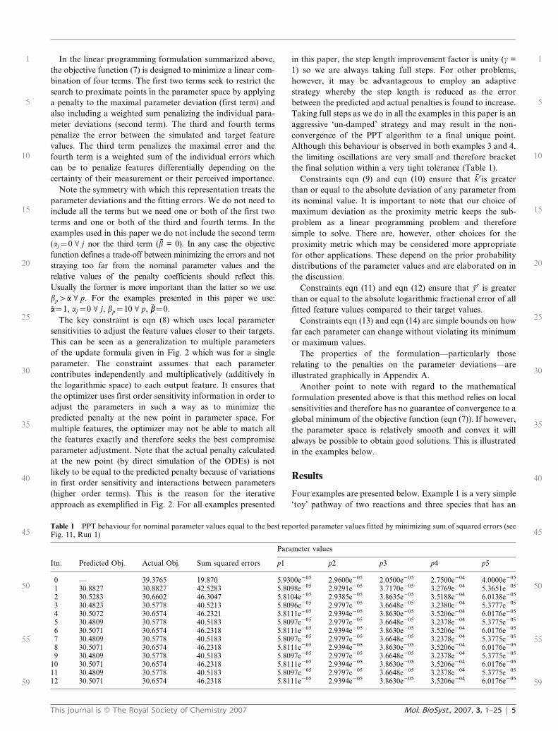
Although this behaviour is observed in both examples 3 and 4.

the limiting oscillations are very small and therefore bracket

the final solution within a very tight tolerance (Table 1).

Constraints eqn (9) and eqn (10) ensure that kris greater

than or equal to the absolute deviation of any parameter from

its nominal value. It is important to note that our choice of

maximum deviation as the proximity metric keeps the sub-

problem as a linear programming problem and therefore

simple to solve. There are, however, other choices for the

proximity metric which may be considered more appropriate

for other applications. These depend on the prior probability

distributions of the parameter values and are elaborated on in

the discussion.

Constraints eqn (11) and eqn (12) ensure that yr is greater

than or equal to the absolute logarithmic fractional error of all

fitted feature values compared to their target values.

Constraints eqn (13) and eqn (14) are simple bounds on how

far each parameter can change without violating its minimum

or maximum values.

The properties of the formulation—particularly those

relating to the penalties on the parameter deviations—are

illustrated graphically in Appendix A.

Another point to note with regard to the mathematical

formulation presented above is that this method relies on local

sensitivities and therefore has no guarantee of convergence to a

global minimum of the objective function (eqn (7)). If however,

the parameter space is relatively smooth and convex it will

always be possible to obtain good solutions. This is illustrated

in the examples below.

Results

Four examples are presented below. Example 1 is a very simple

‘toy’ pathway of two reactions and three species that has an

Table 1 PPT behaviour for nominal parameter values equal to the best reported parameter values fitted by minimizing sum of squared errors (seeFig. 11, Run 1)

Itn. Predicted Obj. Actual Obj. Sum squared errors

Parameter values

p1 p2 p3 p4 p5

0 — 39.3765 19.870 5.9300e205 2.9600e205 2.0500e205 2.7500e204 4.0000e205

1 30.8827 30.8827 42.5283 5.8098e205 2.9291e205 3.7170e205 3.2769e204 5.3651e205

2 30.5283 30.6602 46.3047 5.8104e205 2.9385e205 3.8635e205 3.5188e204 6.0138e205

3 30.4823 30.5778 40.5213 5.8096e205 2.9797e205 3.6648e205 3.2380e204 5.3777e205

4 30.5072 30.6574 46.2321 5.8111e205 2.9394e205 3.8630e205 3.5206e204 6.0176e205

5 30.4809 30.5778 40.5183 5.8097e205 2.9797e205 3.6648e205 3.2378e204 5.3775e205

6 30.5071 30.6574 46.2318 5.8111e205 2.9394e205 3.8630e205 3.5206e204 6.0176e205

7 30.4809 30.5778 40.5183 5.8097e205 2.9797e205 3.6648e205 3.2378e204 5.3775e205

8 30.5071 30.6574 46.2318 5.8111e205 2.9394e205 3.8630e205 3.5206e204 6.0176e205

9 30.4809 30.5778 40.5183 5.8097e205 2.9797e205 3.6648e205 3.2378e204 5.3775e205

10 30.5071 30.6574 46.2318 5.8111e205 2.9394e205 3.8630e205 3.5206e204 6.0176e205

11 30.4809 30.5778 40.5183 5.8097e205 2.9797e205 3.6648e205 3.2378e204 5.3775e205

12 30.5071 30.6574 46.2318 5.8111e205 2.9394e205 3.8630e205 3.5206e204 6.0176e205


1

5

10

15

20

25

30

35

40

45

50

55

59

1

5

10

15

20

25

30

35

40

45

50

55

59

analytical solution and that we use to illustrate the proximate

tuning methodology. In Example 2 we apply the technique to a

model of the p38 MAP kinase signalling pathway for which

very little measured data exist and which is therefore highly

under-constrained. Conversely, in Example 3 we investigate

the performance of the algorithm in a much more constrained

application in which we seek to fit most of the steady state

concentrations in a well-known glycolysis model. This example

also demonstrates the convergence of the method starting from

different nominal points in the parameter space. Finally, in

Example 4 we apply the algorithm to an extensively studied

parameter estimation problem that enables us to compare it to

existing approaches. All examples were solved using Sentero, a

software tool for the modeling and analysis of biochemical

networks that includes the LP-PPT algorithm as one of its

analysis modules. Sentero uses Matlab as the simulation

engine and a third party solver to solve the linear program-

ming sub-problems.

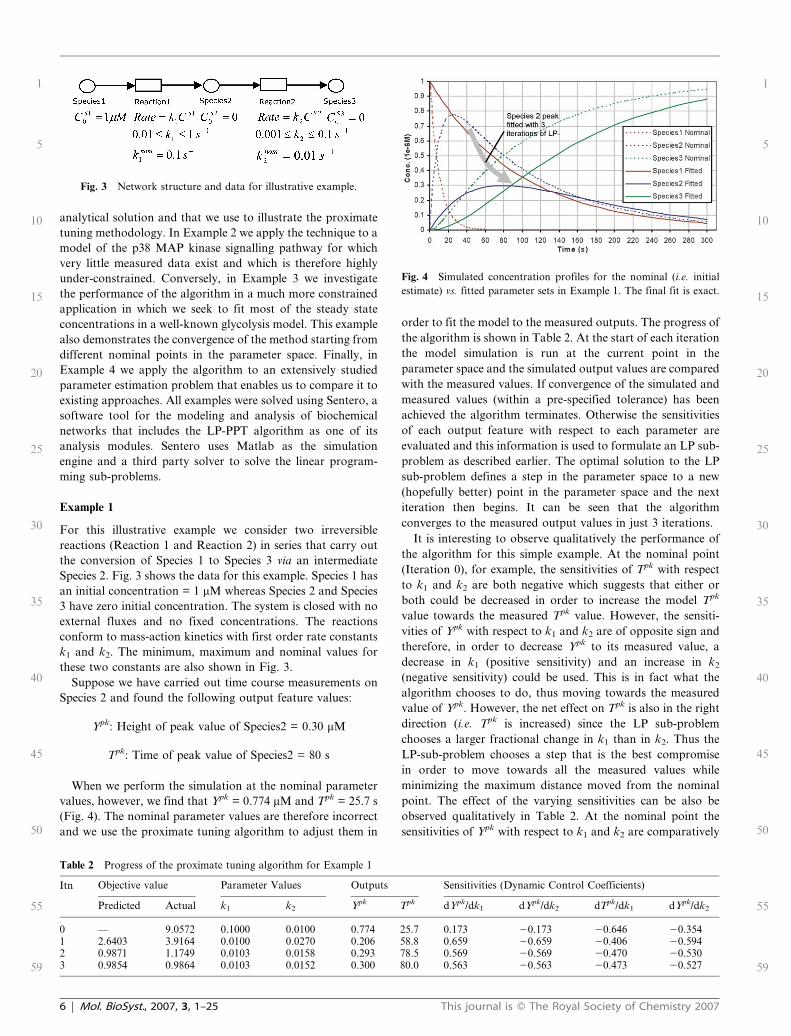
Example 1

For this illustrative example we consider two irreversible

reactions (Reaction 1 and Reaction 2) in series that carry out

the conversion of Species 1 to Species 3 via an intermediate

Species 2. Fig. 3 shows the data for this example. Species 1 has

an initial concentration = 1 mM whereas Species 2 and Species

3 have zero initial concentration. The system is closed with no

external fluxes and no fixed concentrations. The reactions

conform to mass-action kinetics with first order rate constants

k1 and k2. The minimum, maximum and nominal values for

these two constants are also shown in Fig. 3.

Suppose we have carried out time course measurements on

Species 2 and found the following output feature values:

Ypk: Height of peak value of Species2 = 0.30 mM

Tpk: Time of peak value of Species2 = 80 s

When we perform the simulation at the nominal parameter

values, however, we find that Ypk = 0.774 mM and Tpk = 25.7 s

(Fig. 4). The nominal parameter values are therefore incorrect

and we use the proximate tuning algorithm to adjust them in

order to fit the model to the measured outputs. The progress of

the algorithm is shown in Table 2. At the start of each iteration

the model simulation is run at the current point in the

parameter space and the simulated output values are compared

with the measured values. If convergence of the simulated and

measured values (within a pre-specified tolerance) has been

achieved the algorithm terminates. Otherwise the sensitivities

of each output feature with respect to each parameter are

evaluated and this information is used to formulate an LP sub-

problem as described earlier. The optimal solution to the LP

sub-problem defines a step in the parameter space to a new

(hopefully better) point in the parameter space and the next

iteration then begins. It can be seen that the algorithm

converges to the measured output values in just 3 iterations.

It is interesting to observe qualitatively the performance of

the algorithm for this simple example. At the nominal point

(Iteration 0), for example, the sensitivities of Tpk with respect

to k1 and k2 are both negative which suggests that either or

both could be decreased in order to increase the model Tpk

value towards the measured Tpk value. However, the sensiti-

vities of Ypk with respect to k1 and k2 are of opposite sign and

therefore, in order to decrease Ypk to its measured value, a

decrease in k1 (positive sensitivity) and an increase in k2

(negative sensitivity) could be used. This is in fact what the

algorithm chooses to do, thus moving towards the measured

value of Ypk. However, the net effect on Tpk is also in the right

direction (i.e. Tpk is increased) since the LP sub-problem

chooses a larger fractional change in k1 than in k2. Thus the

LP-sub-problem chooses a step that is the best compromise

in order to move towards all the measured values while

minimizing the maximum distance moved from the nominal

point. The effect of the varying sensitivities can be also be

observed qualitatively in Table 2. At the nominal point the

sensitivities of Ypk with respect to k1 and k2 are comparatively

Fig. 3 Network structure and data for illustrative example.

Fig. 4 Simulated concentration profiles for the nominal (i.e. initial

estimate) vs. fitted parameter sets in Example 1. The final fit is exact.

Table 2 Progress of the proximate tuning algorithm for Example 1

Itn Objective value Parameter Values Outputs Sensitivities (Dynamic Control Coefficients)

Predicted Actual k1 k2 Ypk Tpk dYpk/dk1 dYpk/dk2 dTpk/dk1 dYpk/dk2

0 — 9.0572 0.1000 0.0100 0.774 25.7 0.173 20.173 20.646 20.3541 2.6403 3.9164 0.0100 0.0270 0.206 58.8 0.659 20.659 20.406 20.5942 0.9871 1.1749 0.0103 0.0158 0.293 78.5 0.569 20.569 20.470 20.5303 0.9854 0.9864 0.0103 0.0152 0.300 80.0 0.563 20.563 20.473 20.527


1

5

10

15

20

25

30

35

40

45

50

55

59

1

5

10

15

20

25

30

35

40

45

50

55

59

low (¡ 0.173) and the consequence of this is that the LP sub-

problem prescribes the largest possible reduction of k1 down to

its minimum value of 0.01 s21. However, the magnitude of the

Ypk sensitivities increase strongly to (¡ 0.659) at the next point

(Iteration 1). This is indicated by the fact that the algorithm

overestimates that required step and the value of Ypk at the new

point (0.206 mM) is less than its measured value (0.300 mM).

During the next step (Iteration 2) the algorithm corrects this by

slightly increasing the value of k1 from its minimum value.

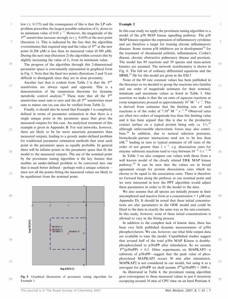
The progress of the algorithm through this 2-dimensional

parameter space is conveniently represented in graphical form

in Fig. 5. Note that the final two points (Iterations 2 and 3) are

difficult to distinguish since they are in close proximity.

Another fact that is evident from Table 2 is that the Ypk

sensitivities are always equal and opposite. This is a

demonstration of the summation theorems for dynamic

metabolic control analysis.18 These state that all the Ypk

sensitivities must sum to zero and the all Tpk sensitivities must

sum to minus one (as can also be verified from Table 2).

Finally, it should also be noted that Example 1 is completely

defined in terms of parameter estimation in that there is a

single unique point in the parameter space that gives the

measured outputs for this case. An analytical treatment of this

example is given in Appendix B. For real networks, however,

there are likely to be far more uncertain parameters than

measured outputs, leading to a grossly under-defined problem

for traditional parameter estimation methods that treat each

point in the parameter space as equally probable. In general

there will be infinite points in the parameter space that fit the

model to the measured outputs. The use of the nominal point

by the proximate tuning algorithm is the key feature that

enables an under-defined problem to be converted into one

that is much better defined—perhaps with a unique solution—

since not all the points fitting the measured values are likely to

be equidistant from the nominal point.

Example 2

In this case study we apply the proximate tuning algorithm to a

model of the p38 MAP kinase signalling pathway. The p38

MAP kinases regulate the expression of inflammatory cytokines

and are therefore a target for treating chronic inflammatory

diseases. Some sixteen p38 inhibitors are in development32 for

the treatment of rheumatoid arthritis, inflammation, Crohn’s

disease, chronic obstructive pulmonary disease and psoriasis.

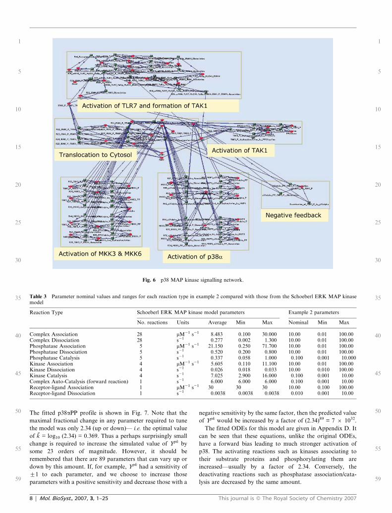
The model has 89 reactions and 59 species and mass-action

kinetics are assumed. The network stoichiometry is shown in

Fig. 6. The full set of ordinary differential equations and the

SBML33 file for this model are given in the ESI.{None of the 89 rate constant values has been published in

the literature so we decided to group the reactions into families

and use order of magnitude estimates for their nominal,

minimum and maximum values as listed in Table 3. One

assertion we make is that the on rates of aqueous reactions at

room temperature proceed at approximately 107 M21 s21. This

is derived from estimates that the limiting rate of such

reactions is of the order of 7.109 M21 s21.34 Observed rates

are often two orders of magnitude less than this limiting value

and it has been argued that this is due to the productive

contact surface on a typical protein being only ca. 1%,35

although unfavourable electrostatic forces may also contri-

bute.36 In addition, due to natural selection pressures,

biomolecule–partner interactions tend not to be less than

nM,37 leading in turn to typical estimates of off rates of the

order of not greater than 1 s21. e.g. dissociation rates for

enzyme–substrate reactions tend to vary between 1024–1 s21.38

In Table 3 we also compare our values with those from a

well known model of the closely related ERK MAP kinase

pathway.39 It can be seen that the values are in broad

agreement except for protein dissociation rates which we

choose to be equal to the association rates. There is therefore

no forward bias along the pathway at our nominal point and

we were interested in how the PPT algorithm would adjust

these parameters in order to fit the model to the data.

We also assume that all species are initially present in their

uncomplexed and inactive form at a concentration = 1 mM (see

Appendix D). It should be noted that these initial concentra-

tions are also parameters in the ODE model and could be

fitted to the data in exactly the same way as the rate constants.

In this study, however, none of these initial concentrations is

allowed to vary in the fitting process.

In addition to the complete lack of kinetic data, there has

been very little published dynamic measurements of p38a

phosphorylation. We can, however, use what little output data

are available to tune the model. Unpublished studies suggest

that around half of the total p38a MAP Kinase is doubly-

phosphorylated to p38aPP after stimulation. So we assume

Ypk(p38aPP) = 0.5. Other experiments on MAPKAP2—a

substrate of p38aPP—suggest that the peak value of phos-

phorylated MAPKAP2 occurs 30 min after stimulation.

MAPKAP2 is not considered in our model, but using it as a

surrogate for p38aPP we shall assume Tpk(p38aPP) = 1800 s.

As illustrated in Table 4, the proximate tuning algorithm

gave convergence to these measured values in just 6 iterations

occupying around 10 min of CPU time on an Intel Pentium 4.

Fig. 5 Graphical illustration of proximate tuning algorithm for

Example 1.


1

5

10

15

20

25

30

35

40

45

50

55

59

1

5

10

15

20

25

30

35

40

45

50

55

59

The fitted p38aPP profile is shown in Fig. 7. Note that the

maximal fractional change in any parameter required to tune

the model was only 2.34 (up or down)— i.e. the optimal value

of k = log10 (2.34) = 0.369. Thus a perhaps surprisingly small

change is required to increase the simulated value of Ypk by

some 23 orders of magnitude. However, it should be

remembered that there are 89 parameters that can vary up or

down by this amount. If, for example, Ypk had a sensitivity of

¡1 to each parameter, and we choose to increase those

parameters with a positive sensitivity and decrease those with a

negative sensitivity by the same factor, then the predicted value

of Ypk would be increased by a factor of (2.34)89 = 7 6 1032.

The fitted ODEs for this model are given in Appendix D. It

can be seen that these equations, unlike the original ODEs,

have a forward bias leading to much stronger activation of

p38. The activating reactions such as kinases associating to

their substrate proteins and phosphorylating them are

increased—usually by a factor of 2.34. Conversely, the

deactivating reactions such as phosphatase association/cata-

lysis are decreased by the same amount.

Fig. 6 p38 MAP kinase signalling network.

Table 3 Parameter nominal values and ranges for each reaction type in example 2 compared with those from the Schoeberl ERK MAP kinasemodel

Reaction Type Schoeberl ERK MAP kinase model parameters Example 2 parameters

No. reactions Units Average Min Max Nominal Min Max

Complex Association 28 mM21 s21 8.483 0.100 30.000 10.00 0.01 100.00Complex Dissociation 28 s21 0.277 0.002 1.300 10.00 0.01 100.00Phosphatase Association 5 mM21 s21 21.150 0.250 71.700 10.00 0.01 100.00Phosphatase Dissociation 5 s21 0.520 0.200 0.800 10.00 0.01 100.00Phosphatase Catalysis 5 s21 0.337 0.058 1.000 0.100 0.001 10.000Kinase Association 4 mM21 s21 5.605 0.110 11.100 10.00 0.01 100.00Kinase Dissociation 4 s21 0.026 0.018 0.033 10.00 0.010 100.00Kinase Catalysis 4 s21 7.025 2.900 16.000 0.100 0.001 10.00Complex Auto-Catalysis (forward reaction) 1 s21 6.000 6.000 6.000 0.100 0.001 10.00Receptor-ligand Association 1 mM21 s21 30 30 30 10.00 0.100 100.00Receptor-ligand Dissociation 1 s21 0.0038 0.0038 0.0038 0.010 0.001 10.00


1

5

10

15

20

25

30

35

40

45

50

55

59

1

5

10

15

20

25

30

35

40

45

50

55

59

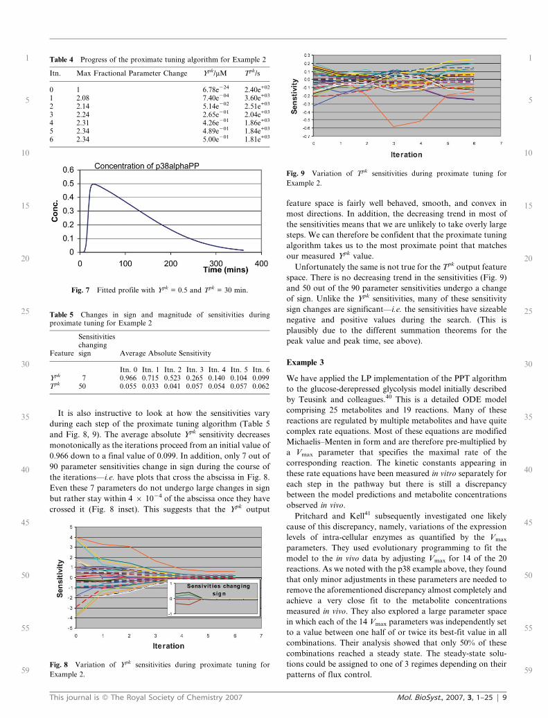
It is also instructive to look at how the sensitivities vary

during each step of the proximate tuning algorithm (Table 5

and Fig. 8, 9). The average absolute Ypk sensitivity decreases

monotonically as the iterations proceed from an initial value of

0.966 down to a final value of 0.099. In addition, only 7 out of

90 parameter sensitivities change in sign during the course of

the iterations—i.e. have plots that cross the abscissa in Fig. 8.

Even these 7 parameters do not undergo large changes in sign

but rather stay within 4 6 1024 of the abscissa once they have

crossed it (Fig. 8 inset). This suggests that the Ypk output

feature space is fairly well behaved, smooth, and convex in

most directions. In addition, the decreasing trend in most of

the sensitivities means that we are unlikely to take overly large

steps. We can therefore be confident that the proximate tuning

algorithm takes us to the most proximate point that matches

our measured Ypk value.

Unfortunately the same is not true for the Tpk output feature

space. There is no decreasing trend in the sensitivities (Fig. 9)

and 50 out of the 90 parameter sensitivities undergo a change

of sign. Unlike the Ypk sensitivities, many of these sensitivity

sign changes are significant—i.e. the sensitivities have sizeable

negative and positive values during the search. (This is

plausibly due to the different summation theorems for the

peak value and peak time, see above).

Example 3

We have applied the LP implementation of the PPT algorithm

to the glucose-derepressed glycolysis model initially described

by Teusink and colleagues.40 This is a detailed ODE model

comprising 25 metabolites and 19 reactions. Many of these

reactions are regulated by multiple metabolites and have quite

complex rate equations. Most of these equations are modified

Michaelis–Menten in form and are therefore pre-multiplied by

a Vmax parameter that specifies the maximal rate of the

corresponding reaction. The kinetic constants appearing in

these rate equations have been measured in vitro separately for

each step in the pathway but there is still a discrepancy

between the model predictions and metabolite concentrations

observed in vivo.

Pritchard and Kell41 subsequently investigated one likely

cause of this discrepancy, namely, variations of the expression

levels of intra-cellular enzymes as quantified by the Vmax

parameters. They used evolutionary programming to fit the

model to the in vivo data by adjusting Vmax for 14 of the 20

reactions. As we noted with the p38 example above, they found

that only minor adjustments in these parameters are needed to

remove the aforementioned discrepancy almost completely and

achieve a very close fit to the metabolite concentrations

measured in vivo. They also explored a large parameter space

in which each of the 14 Vmax parameters was independently set

to a value between one half of or twice its best-fit value in all

combinations. Their analysis showed that only 50% of these

combinations reached a steady state. The steady-state solu-

tions could be assigned to one of 3 regimes depending on their

patterns of flux control.

Table 4 Progress of the proximate tuning algorithm for Example 2

Itn. Max Fractional Parameter Change Ypk/mM Tpk/s

0 1 6.78e224 2.40e+02

1 2.08 7.40e204 3.60e+03

2 2.14 5.14e202 2.51e+03

3 2.24 2.65e201 2.04e+03

4 2.31 4.26e201 1.86e+03

5 2.34 4.89e201 1.84e+03

6 2.34 5.00e201 1.81e+03

Fig. 7 Fitted profile with Ypk = 0.5 and Tpk = 30 min.

Table 5 Changes in sign and magnitude of sensitivities duringproximate tuning for Example 2

Feature

Sensitivitieschangingsign Average Absolute Sensitivity

Itn. 0 Itn. 1 Itn. 2 Itn. 3 Itn. 4 Itn. 5 Itn. 6Ypk 7 0.966 0.715 0.523 0.265 0.140 0.104 0.099Tpk 50 0.055 0.033 0.041 0.057 0.054 0.057 0.062

Fig. 8 Variation of Ypk sensitivities during proximate tuning for

Example 2.

Fig. 9 Variation of Tpk sensitivities during proximate tuning for

Example 2.


1

5

10

15

20

25

30

35

40

45

50

55

59

1

5

10

15

20

25

30

35

40

45

50

55

59

This parameter space, together with the requirement to fit 12

steady-state variables represents a challenging landscape and

we decided to use it to test the PPT algorithm. We were

interested in whether the algorithm could start at randomly

selected points within the parameter space and navigate to the

best fit point that matches the target metabolite concentra-

tions. We randomly sampled 20 points from within the same

parameter space as considered by Pritchard and Kell.41 Note

that they were exploring the vertices of the parameter space

hypercube whereas we sampled uniformly from its interior.

We found that 12 out of the 20 (60%) sampled nominal

points achieved a steady state, which is in broad agreement

with the figure of 50% reported by Pritchard and Kell although

they were sampling from the edge of the parameter space

rather then uniformly from its interior as in this work. The LP-

PPT algorithm achieved a reasonable fit for 11 out of the 20

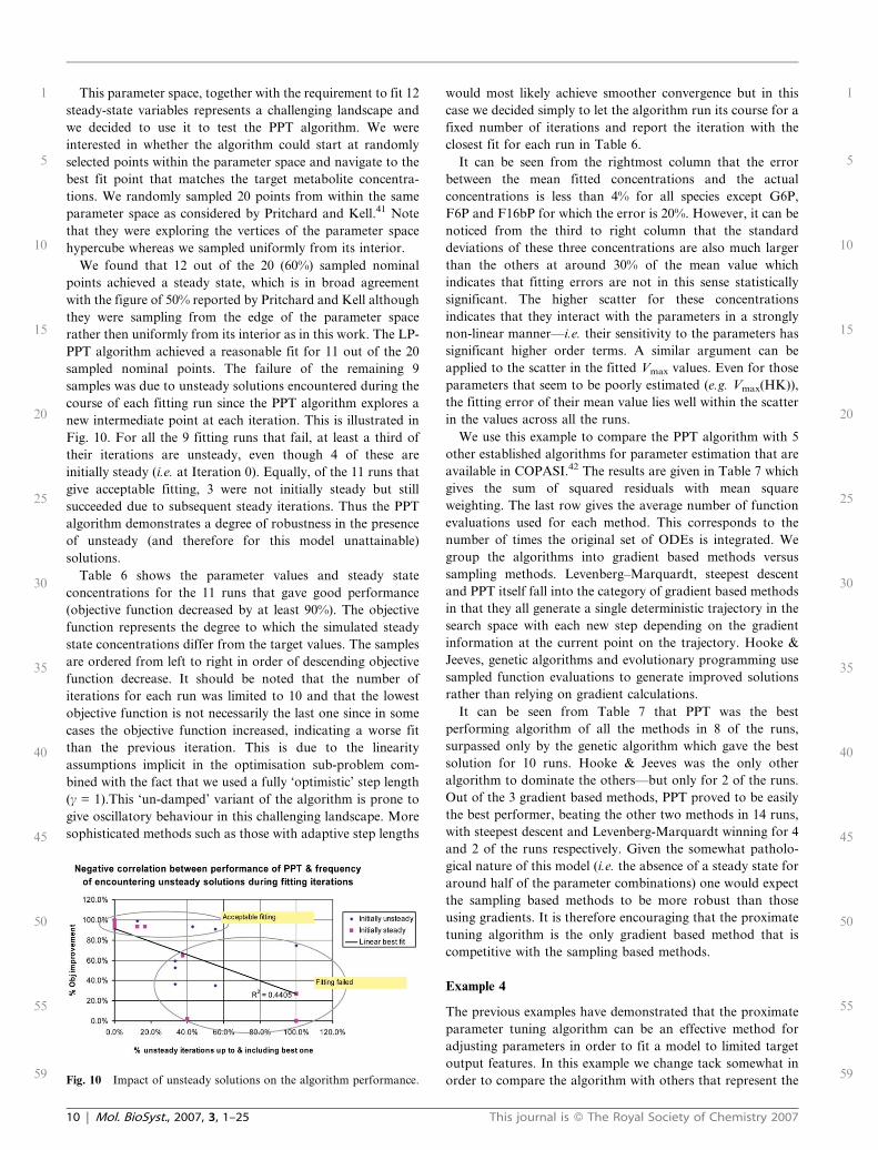
sampled nominal points. The failure of the remaining 9

samples was due to unsteady solutions encountered during the

course of each fitting run since the PPT algorithm explores a

new intermediate point at each iteration. This is illustrated in

Fig. 10. For all the 9 fitting runs that fail, at least a third of

their iterations are unsteady, even though 4 of these are

initially steady (i.e. at Iteration 0). Equally, of the 11 runs that

give acceptable fitting, 3 were not initially steady but still

succeeded due to subsequent steady iterations. Thus the PPT

algorithm demonstrates a degree of robustness in the presence

of unsteady (and therefore for this model unattainable)

solutions.

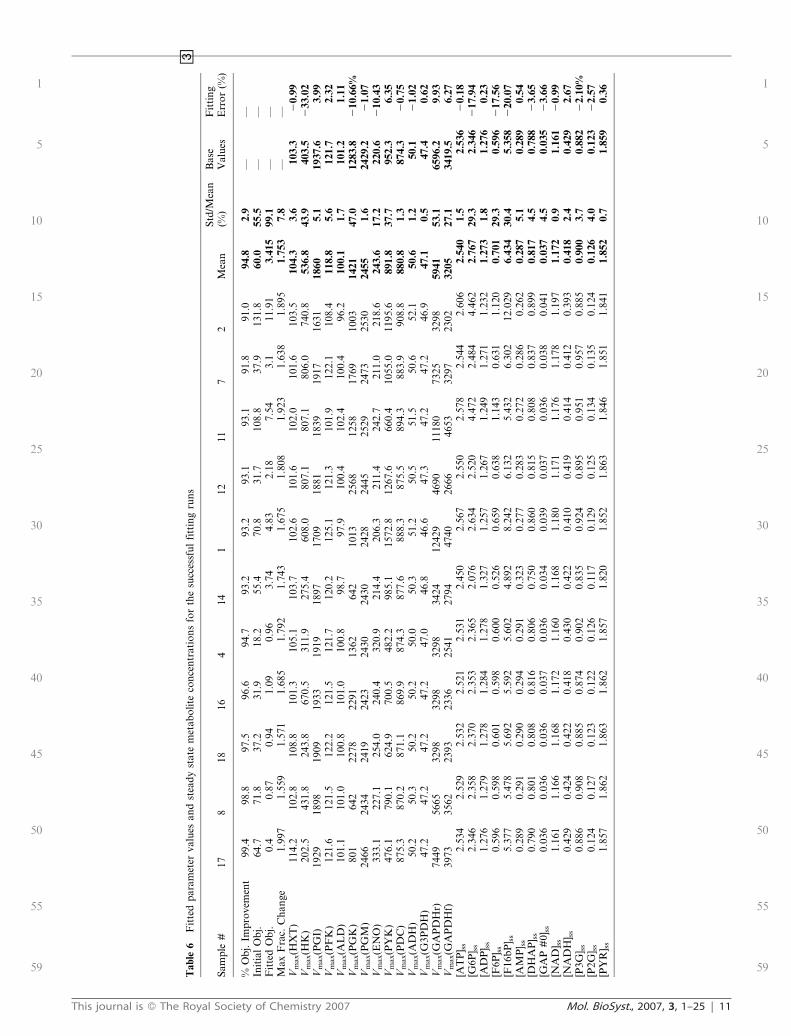
Table 6 shows the parameter values and steady state

concentrations for the 11 runs that gave good performance

(objective function decreased by at least 90%). The objective

function represents the degree to which the simulated steady

state concentrations differ from the target values. The samples

are ordered from left to right in order of descending objective

function decrease. It should be noted that the number of

iterations for each run was limited to 10 and that the lowest

objective function is not necessarily the last one since in some

cases the objective function increased, indicating a worse fit

than the previous iteration. This is due to the linearity

assumptions implicit in the optimisation sub-problem com-

bined with the fact that we used a fully ‘optimistic’ step length

(c = 1).This ‘un-damped’ variant of the algorithm is prone to

give oscillatory behaviour in this challenging landscape. More

sophisticated methods such as those with adaptive step lengths

would most likely achieve smoother convergence but in this

case we decided simply to let the algorithm run its course for a

fixed number of iterations and report the iteration with the

closest fit for each run in Table 6.

It can be seen from the rightmost column that the error

between the mean fitted concentrations and the actual

concentrations is less than 4% for all species except G6P,

F6P and F16bP for which the error is 20%. However, it can be

noticed from the third to right column that the standard

deviations of these three concentrations are also much larger

than the others at around 30% of the mean value which

indicates that fitting errors are not in this sense statistically

significant. The higher scatter for these concentrations

indicates that they interact with the parameters in a strongly

non-linear manner—i.e. their sensitivity to the parameters has

significant higher order terms. A similar argument can be

applied to the scatter in the fitted Vmax values. Even for those

parameters that seem to be poorly estimated (e.g. Vmax(HK)),

the fitting error of their mean value lies well within the scatter

in the values across all the runs.

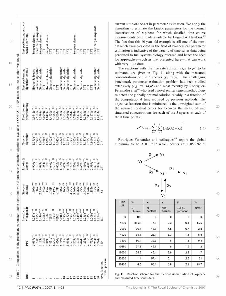
We use this example to compare the PPT algorithm with 5

other established algorithms for parameter estimation that are

available in COPASI.42 The results are given in Table 7 which

gives the sum of squared residuals with mean square

weighting. The last row gives the average number of function

evaluations used for each method. This corresponds to the

number of times the original set of ODEs is integrated. We

group the algorithms into gradient based methods versus

sampling methods. Levenberg–Marquardt, steepest descent

and PPT itself fall into the category of gradient based methods

in that they all generate a single deterministic trajectory in the

search space with each new step depending on the gradient

information at the current point on the trajectory. Hooke &

Jeeves, genetic algorithms and evolutionary programming use

sampled function evaluations to generate improved solutions

rather than relying on gradient calculations.

It can be seen from Table 7 that PPT was the best

performing algorithm of all the methods in 8 of the runs,

surpassed only by the genetic algorithm which gave the best

solution for 10 runs. Hooke & Jeeves was the only other

algorithm to dominate the others—but only for 2 of the runs.

Out of the 3 gradient based methods, PPT proved to be easily

the best performer, beating the other two methods in 14 runs,

with steepest descent and Levenberg-Marquardt winning for 4

and 2 of the runs respectively. Given the somewhat patholo-

gical nature of this model (i.e. the absence of a steady state for

around half of the parameter combinations) one would expect

the sampling based methods to be more robust than those

using gradients. It is therefore encouraging that the proximate

tuning algorithm is the only gradient based method that is

competitive with the sampling based methods.

Example 4

The previous examples have demonstrated that the proximate

parameter tuning algorithm can be an effective method for

adjusting parameters in order to fit a model to limited target

output features. In this example we change tack somewhat in

order to compare the algorithm with others that represent theFig. 10 Impact of unsteady solutions on the algorithm performance.


1

5

10

15

20

25

30

35

40

45

50

55

59

1

5

10

15

20

25

30

35

40

45

50

55

59

Ta

ble

6F

itte

dp

ara

met

ervalu

esan

dst

ead

yst

ate

met

ab

oli

teco

nce

ntr

ati

on

sfo

rth

esu

cces

sfu

lfi

ttin

gru

ns

=

Sa

mp

le#

17

81

81

64

14

11

21

17

2M

ean

Std

/Mea

n(%

)B

ase

Va

lues

Fit

tin

gE

rro

r(%

)

%O

bj.

Imp

rov

emen

t9

9.4

98

.89

7.5

96

.69

4.7

93

.29

3.2

93

.19

3.1

91

.89

1.0

94

.82

.9—

—In

itia

lO

bj.

64

.77

1.8

37

.23

1.9

18

.25

5.4

70

.83

1.7

10

8.8

37

.91

31

.86

0.0

55

.5—

—F

itte

dO

bj.

0.4

0.8

70.9

41.0

90.9

63.7

44.8

32.1

87.5

43.1

11.9

13

.41

59

9.1

——

Ma

xF

rac.

Ch

an

ge

1.9

97

1.5

59

1.5

71

1.6

85

1.7

92

1.7

43

1.6

75

1.8

08

1.9

23

1.6

38

1.8

95

1.7

53

7.8

——

Vm

ax(H

XT

)1

14

.21

02

.81

08

.81

01

.31

05

.11

03

.71

02

.61

01

.61

02

.01

01

.61

03

.51

04

.33

.61

03

.32

0.9

9V

max(H

K)

20

2.5

43

1.8

24

3.8

67

0.5

31

1.9

27

5.4

60

8.0

80

7.1

80

7.1

80

6.0

74

0.8

53

6.8

43

.94

03

.52

33

.02

Vm

ax(P

GI)

19

29

18

98

19

09

19

33

19

19

18

97

17

09

18

81

18

39

19

17

16

31

18

60

5.1

19

37.6

3.9

9V

max(P

FK

)1

21

.61

21

.51

22

.21

21

.51

21

.71

20

.21

25

.11

21

.31

01

.91

22

.11

08

.41

18

.85

.61

21

.72

.32

Vm

ax(A

LD

)1

01

.11

01

.01

00

.81

01

.01

00

.89

8.7

97

.91

00

.41

02

.41

00

.49

6.2

10

0.1

1.7

10

1.2

1.1

1V

max(P

GK

)8

01

64

22

27

82

29

11

36

26

42

10

13

25

68

12

58

17

69

10

03

14

21

47

.01

28

3.8

21

0.6

6%

Vm

ax(P

GM

)2

46

62

43

42

41

92

42

32

43

02

43

02

42

82

44

52

52

92

47

32

53

02

45

51

.62

42

9.2

21

.07

Vm

ax(E

NO

)3

33

.12

27

.12

54

.02

40

.43

20

.92

14

.42

06

.32

11

.42

42

.72

11

.02

18

.62

43

.61

7.2

22

0.6

21

0.4

3V

max(P

YK

)4

76

.17

90

.16

24

.97

00

.54

82

.29

85

.11

57

2.8

12

67.6

66

0.4

10

55

.01

19

5.6

89

1.8

37

.79

52

.36

.35

Vm

ax(P

DC

)8

75

.38

70

.28

71

.18

69

.98

74

.38

77

.68

88

.38

75

.58

94

.38

83

.99

08

.88

80

.81

.38

74

.32

0.7

5V

max(A

DH

)5

0.2

50

.35

0.2

50

.25

0.0

50

.35

1.2

50

.55

1.5

50

.65

2.1

50

.61

.25

0.1

21

.02

Vm

ax(G

3P

DH

)4

7.2

47

.24

7.2

47

.24

7.0

46

.84

6.6

47

.34

7.2

47

.24

6.9

47

.10

.54

7.4

0.6

2V

max(G

AP

DH

r)7

44

95

66

53

29

83

29

83

29

83

42

41

24

29

46

90

11

180

73

25

32

98

59

41

53

.16

59

6.2

9.9

3V

max(G

AP

DH

f)3

97

33

56

22

39

32

33

62

54

12

79

44

74

02

66

64

65

33

29

72

30

23

20

52

7.1

34

19.5

6.2

7[A

TP

] ss

2.5

34

2.5

29

2.5

32

2.5

21

2.5

31

2.4

50

2.5

67

2.5

50

2.5

78

2.5

44

2.6

06

2.5

40

1.5

2.5

36

20

.18

[G6

P] s

s2

.34

62

.35

82

.37

02

.35

32

.36

52

.07

62

.63

42

.52

04

.47

22

.48

44

.46

22

.76

72

9.3

2.3

46

21

7.9

4[A

DP

] ss

1.2

76

1.2

79

1.2

78

1.2

84

1.2

78

1.3

27

1.2

57

1.2

67

1.2

49

1.2

71

1.2

32

1.2

73

1.8

1.2

76

0.2

3[F

6P

] ss

0.5

96

0.5

98

0.6

01

0.5

98

0.6

00

0.5

26

0.6

59

0.6

38

1.1

43

0.6

31

1.1

20

0.7

01

29

.30

.59

62

17

.56

[F1

6b

P] s

s5

.37

75

.47

85

.69

25

.59

25

.60

24

.89

28

.24

26

.13

25

.43

26

.30

21

2.0

29

6.4

34

30

.45

.35

82

20

.07

[AM

P] s

s0

.28

90

.29

10

.29

00

.29

40

.29

10

.32

30

.27

70

.28

30

.27

20

.28

60

.26

20

.28

75

.10

.28

90

.54

[DH

AP

] ss

0.7

90

0.8

01

0.8

08

0.8

16

0.8

06

0.7

50

0.8

60

0.8

15

0.8

08

0.8

37

0.8

99

0.8

17

4.5

0.7

88

23

.65

[GA

P#

0] s

s0

.03

60

.03

60

.03

60

.03

70

.03

60

.03

40

.03

90

.03

70

.03

60

.03

80

.04

10

.03

74

.50

.03

52

3.6

6[N

AD

] ss

1.1

61

1.1

66

1.1

68

1.1

72

1.1

60

1.1

68

1.1

80

1.1

71

1.1

76

1.1

78

1.1

97

1.1

72

0.9

1.1

61

20

.99

[NA

DH

] ss

0.4

29

0.4

24

0.4

22

0.4

18

0.4

30

0.4

22

0.4

10

0.4

19

0.4

14

0.4

12

0.3

93

0.4

18

2.4

0.4

29

2.6

7[P

3G

] ss

0.8

86

0.9

08

0.8

85

0.8

74

0.9

02

0.8

35

0.9

24

0.8

95

0.9

51

0.9

57

0.8

85

0.9

00

3.7

0.8

82

22

.10

%[P

2G

] ss

0.1

24

0.1

27

0.1

23

0.1

22

0.1

26

0.1

17

0.1

29

0.1

25

0.1

34

0.1

35

0.1

24

0.1

26

4.0

0.1

23

22

.57

[PY

R] s

s1

.85

71

.86

21

.86

31

.86

21

.85

71

.82

01

.85

21

.86

31

.84

61

.85

11

.84

11

.85

20

.71

.85

90

.36


1

5

10

15

20

25

30

35

40

45

50

55

59

1

5

10

15

20

25

30

35

40

45

50

55

59

current state-of-the-art in parameter estimation. We apply the

algorithm to estimate the kinetic parameters for the thermal

isomerisation of a-pinene for which detailed time course

measurements been made available by Fuguitt & Hawkins.43

The fact that this 60-year-old example is still one of the most

data-rich examples cited in the field of biochemical parameter

estimation is indicative of the paucity of time series data being

generated to fuel systems biology research and hence the need

for approaches—such as that presented here—that can work

with very little data.

The reactions with the five rate constants (p1 to p5) to be

estimated are given in Fig. 11 along with the measured

concentrations of the 5 species (y1 to y5). This challenging

benchmark parameter estimation problem has been studied

extensively (e.g. ref. 44,45) and most recently by Rodriguez-

Fernandez et al46 who used a novel scatter search methodology

to detect the globally optimal solution reliably in a fraction of

the computational time required by previous methods. The

objective function that is minimized is the unweighted sum of

the squared residual errors for between the measured and

simulated concentrations for each of the 5 species at each of

the 8 time points:

JSSR pð Þ~X5

j~1

X8

i~1

yj p,tið Þ{~yyji

� �2

(16)

Rodriguez-Fernandez and colleagues46 report the global

minimum to be J = 19.87 which occurs at: p1=5.926e25,

Ta

ble

7C

om

pari

son

of

the

pro

xim

ate

pa

ram

eter

tun

ing

alg

ori

thm

wit

h5

pa

ram

eter

esti

ma

tio

na

lgo

rith

ms

av

ail

ab

lein

CO

PA

SI.

#IN

Fm

ean

sth

at

no

solu

tio

nw

as

fou

nd

Ru

nP

PT

Lev

enb

erg

Ma

rqu

ard

tS

teep

est

des

cen

tH

oo

ke

&Je

eves

Gen

etic

alg

ori

thm

Evo

luti

on

ary

pro

gra

mm

ing

Bes

tp

erfo

rmin

galg

ori

thm

over

all

Bes

tp

erfo

rmin

gg

rad

ien

tb

ase

dalg

ori

thm

15

.69

7e2

02

3.2

47e2

01

1.9

09

e202

6.9

09e2

03

1.3

75e2

02

6.0

542

e202

Ho

ok

e&

Jeev

esS

teep

est

des

cen

t2

3.7

98e2

01

1.8

05e2

01

1.6

87

e+00

1.1

91e2

01

3.9

94e2

02

7.5

641

e202

Gen

etic

alg

ori

thm

Lev

enb

erg-m

arq

uard

t3

1.1

33e+

01

2.4

36e+

03

2.4

59

e201

2.0

89e2

02

1.6

67e2

02

3.3

798

e202

Gen

etic

alg

ori

thm

Ste

epes

td

esce

nt

44

.33

8e2

04

1.2

08e2

02

1.8

49

e202

1.2

84e2

02

6.9

30e2

02

8.0

994

e202

PP

TP

PT

52

.81

9e2

01

2.3

60e2

01

1.4

57

e201

1.1

27e2

02

4.6

29e2

02

1.0

499

e201

Ho

ok

e&

Jeev

esS

teep

est

des

cen

t6

7.4

31e+

00

#IN

F#

INF

5.0

40e2

01

3.1

02e2

02

8.4

930

e202

Gen

etic

alg

ori

thm

PP

T7

6.6

86e2

03

2.1

93e2

01

2.1

93

e201

2.5

01e2

02

1.2

63e2

02

5.2

787

e202

PP

TP

PT

81

.42

0e2

04

#IN

F#

INF

9.0

02e2

02

4.0

82e2

02

8.5

003

e202

PP

TP

PT

95

.76

9e2

01

8.0

46e2

01

1.3

02

e+00

8.1

79e2

02

2.2

32e2

02

6.7

386

e202

Gen

etic

alg

ori

thm

PP

T1

07

.11

5e2

01

1.5

85e+

00

1.4

66

e+00

7.4

59e2

01

1.7

17e2

02

2.5

531

e202

Gen

etic

alg

ori

thm

PP

T1

18

.65

4e2

02

1.6

72e+

00

1.6

24

e+00

6.1

93e2

01

2.3

84e2

02

4.9

066

e202

Gen

etic

alg

ori

thm

PP

T1

24

.59

1e2

03

8.5

91e2

01

4.7

53

e202

7.7

77e2

03

2.2

93e2

02

2.5

364

e202

PP

TP

PT

13

5.8

03e2

01

4.5

12e2

01

3.4

67

e201

8.8

76e2

02

9.1

62e2

02

9.7

494

e202

Gen

etic

alg

ori

thm

Ste

epes

td

esce

nt

14

3.3

75e2

03

9.6

49e+

00

6.7

64

e202

7.1

68e2

03

3.5

89e2

02

8.5

433

e202

PP

TP

PT

15

3.4

44e2

01

1.8

48e+

00

1.8

35

e+00

6.6

67e2

02

2.9

77e2

02

1.0

630

e201

Gen

etic

alg

ori

thm

PP

T1

64

.23

4e2

04

1.2

35e+

00

3.9

44

e202

2.4

59e2

03

5.1

57e2

02

5.3

368

e202

PP

TP

PT

17

4.1

05e2

06

3.2

35e2

01

3.2

44

e201

1.4

70e2

01

2.9

15e2

02

6.9

475

e202

PP

TP

PT

18

7.7

33e2

04

1.2

09e+

00

1.1

83

e202

2.3

99e2

02

4.9

10e2

02

5.1

171

e202

PP

TP

PT

19

5.9

84e2

01

4.8

71e2

01

1.2

33

e+00

4.8

71e2

01

2.5

57e2

02

7.1

215

e202

Gen

etic

alg

ori

thm

Lev

enb

erg-m

arq

uard

t2

05

.79

4e2

01

2.8

74e+

02

1.7

00

e+00

2.8

48e2

02

1.6

23e2

02

1.6

233

e202

Gen

etic

alg

ori

thm

PP

TA

ve.

fun

ctio

nev

als

.p

erru

n1

40

18

01

82

27

72

16

21

6—

—

Fig. 11 Reaction scheme for the thermal isomerisation of a-pinene

and measured time series data.


1

5

10

15

20

25

30

35

40

45

50

55

59

1

5

10

15

20

25

30

35

40

45

50

55

59

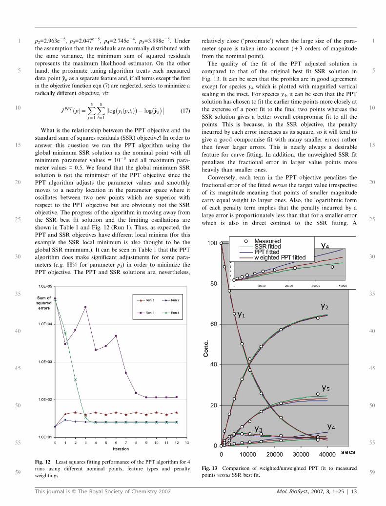
p2=2.963e25, p3=2.047e25, p4=2.745e24, p5=3.998e25. Under

the assumption that the residuals are normally distributed with

the same variance, the minimum sum of squared residuals

represents the maximum likelihood estimator. On the other

hand, the proximate tuning algorithm treats each measured

data point ~yyji as a separate feature and, if all terms except the first

in the objective function eqn (7) are neglected, seeks to minimize a

radically different objective, viz:

JPPT pð Þ~X5

j~1

X8

i~1

log yj p,tið Þ� �

{ log ~yyji

� �� (17)

What is the relationship between the PPT objective and the

standard sum of squares residuals (SSR) objective? In order to

answer this question we ran the PPT algorithm using the

global minimum SSR solution as the nominal point with all

minimum parameter values = 1028 and all maximum para-

meter values = 0.5. We found that the global minimum SSR

solution is not the minimiser of the PPT objective since the

PPT algorithm adjusts the parameter values and smoothly

moves to a nearby location in the parameter space where it

oscillates between two new points which are superior with

respect to the PPT objective but are obviously not the SSR

objective. The progress of the algorithm in moving away from

the SSR best fit solution and the limiting oscillations are

shown in Table 1 and Fig. 12 (Run 1). Thus, as expected, the

PPT and SSR objectives have different local minima (for this

example the SSR local minimum is also thought to be the

global SSR minimum.). It can be seen in Table 1 that the PPT

algorithm does make significant adjustments for some para-

meters (e.g. 88% for parameter p3) in order to minimize the

PPT objective. The PPT and SSR solutions are, nevertheless,

relatively close (‘proximate’) when the large size of the para-

meter space is taken into account (¡3 orders of magnitude

from the nominal point).

The quality of the fit of the PPT adjusted solution is

compared to that of the original best fit SSR solution in

Fig. 13. It can be seen that the profiles are in good agreement

except for species y4 which is plotted with magnified vertical

scaling in the inset. For species y4, it can be seen that the PPT

solution has chosen to fit the earlier time points more closely at

the expense of a poor fit to the final two points whereas the

SSR solution gives a better overall compromise fit to all the

points. This is because, in the SSR objective, the penalty

incurred by each error increases as its square, so it will tend to

give a good compromise fit with many smaller errors rather

then fewer larger errors. This is nearly always a desirable

feature for curve fitting. In addition, the unweighted SSR fit

penalizes the fractional error in larger value points more

heavily than smaller ones.

Conversely, each term in the PPT objective penalizes the

fractional error of the fitted versus the target value irrespective

of its magnitude meaning that points of smaller magnitude

carry equal weight to larger ones. Also, the logarithmic form

of each penalty term implies that the penalty incurred by a

large error is proportionately less than that for a smaller error

which is also in direct contrast to the SSR fitting. A

Fig. 12 Least squares fitting performance of the PPT algorithm for 4

runs using different nominal points, feature types and penalty

weightings.

Fig. 13 Comparison of weighted/unweighted PPT fit to measured

points versus SSR best fit.


1

5

10

15

20

25

30

35

40

45

50

55

59

1

5

10

15

20

25

30

35

40

45

50

55

59

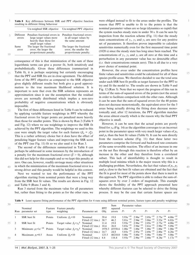
consequence of this is that minimization of the sum of these

logarithmic terms can give a poorer fit, both intuitively and

probabilistically. Given these differences (summarized in

Table 8), it is perhaps surprising but certainly encouraging

that the PPT and SSR fits are in close agreement. The different

form of the PPT objective as compared to the SSR objective

gives slightly different results but both give a good approxi-

mation to the true maximum likelihood solution. It is

important to note that even the SSR solution represents an

approximation since it use the assumption that the residual

errors are normally distributed which implies a non-zero

probability of negative concentrations which is obviously

impossible.

The first of these differences listed in Table 8 can be reduced

by applying variable feature weightings in PPT whereby the

fractional errors for larger points are penalized more heavily

than those for smaller points. This is shown by Run 2 (Table 9

and Fig. 12) where we use weightings to improve the SSR fit

achieved by the PPT algorithm. The weightings we used in this

case were simply the target value for each feature (bp = ygp).

This is a rather arbitrary choice but it does have the effect of

penalizing bigger feature values and improving the SSR score

of the PPT (see Fig. 11) fit so we also used it for Run 3.

The second of the differences summarized in Table 8 can

perhaps be addressed in some instances by the introduction of

a penalty for the maximum fractional error (b . 0), although

this did not help for this example and so we kept this penalty at

zero. One can, however, readily envisage many other situations

in which the minimization of the maximum fractional error is a

strong driver and this penalty would be helpful in this context.

Next we wanted to test the performance of the PPT

algorithm starting from nominal points that were a long way

from the SSR best fit values. The results are shown in Fig. 12

and Table 9 (Runs 3 and 4).

Run 3 started from the maximum value for all parameters

but, rather than fitting to the points as for the other runs, we

were obliged instead to fit to the areas under the profiles. The

reason that PPT is unable to fit to the points is that the

nominal parameter values are so large (dynamics so rapid) that

the system reaches steady state in under 30 s. It can be seen by

inspection from the reaction scheme (Fig. 11) that the steady

state concentrations of y1, y3 and y5 are zero for any positive

set of parameters. It therefore proves impossible to calculate

sensitivities numerically even for the first measured time point

(1020 s) since the steady state has long since been reached. The

concentrations of y1, y3 and y5 are all zero at this time and a

perturbation in any parameter value has no detectable effect

(i.e. their concentrations remain zero). This is all due to a very

poor choice of nominal point.

However, the areas under the concentration profiles have

finite values and sensitivities could be calculated for all of these

species profile areas. We therefore decided to use the total area

under each SSR best fit profile as target features for the PPT to

try and fit the model to. The results are shown in Table 9 and

Fig. 12 (Run 3). Note that we report the progress of this run in

terms of the sum-of-squared errors of the points (not the areas)

in order to facilitate comparison with the other runs. Although

it can be seen that the sum-of-squared errors for the 40 points

does not decrease monotonically, the equivalent error for the 5

areas being actually driving the fitting does decrease mono-

tonically and, after 12 iterations, the PPT algorithm matches

the areas almost exactly which is the reason why the final PPT

objective is small.

However, it can be seen that the actual points are poorly

fitted for y4 (Fig. 14) as the algorithm converges to an incorrect

point in the parameter space with very much larger values of p4

and p5 than the best fit values (Table 9). It can be seen directly

from the reaction scheme (Fig. 11) that these latter two

parameters comprise the forward and backward rate constants

of the same reversible reaction. The effect of an increase in one

on the net flux through this reaction is therefore offset by an

increase in the other and they therefore form a correlated

subset. This lack of identifiability is thought to result in

multiple local minima which is the major reason why this is a

challenging problem. Nevertheless, the fact that values of p1, p2

and p3 close to the best fit values are obtained and the fact that

the fit is good for most of the points show that there is merit in

this approach. The PPT algorithm is able to reduce the sum-of-

squares error by over 2 orders of magnitude. This example

shows the flexibility of the PPT approach presented here

whereby different features can be selected to drive the fitting

process. It may be the case that certain feature spaces are

Table 8 Key differences between SSR and PPT objective functionresulting in different fitting behaviour

Un-weighted SSR objective Un-weighted PPT objective

Differenterrors

Penalises fractional errors inlarge target values moreheavily than those forsmall target values

Penalises fractional errorsin all target values bythe same amount

Sameerror

The larger the fractionalerror, the larger theproportionate penalty.

The larger the fractionalerror, the smaller theproportionate penalty.

Table 9 Least squares fitting performance of the PPT algorithm for 4 runs using different nominal points, feature types and penalty weightings

RunNominalparameter set

Featuretype

Feature penaltyweighting Parameter set

PPTObj.

Sumsquarederrors

Parameter values

p1 p2 p3 p4 p5

1 SSR best fit Points Uniform: bp=10 Nominal 39.4 19.8 5.93e205 2.96e205 2.05e205 2.75e204 4.00e205

Fitted (12 itns.) 30.7 46.2 5.81e205 2.94e205 3.86e205 3.52e204 6.02e205

2 SSR best fit Points Target value: bp=ypg Nominal 11.4 19.8 5.93e205 2.96e205 2.05e205 2.75e204 4.00e205


3 Minimum: pi=1e208 Points Target value: bp=ypg Nominal 1970.3 45558.6 1.00e208 1.00e208 1.00e208 1.00e208 1.00e208


4 Maximum: pi=0.5 Areas Uniform: bp=10 Nominal 125.5 48210.0 5.00e201 5.00e201 5.00e201 5.00e201 5.00e201



1

5

10

15

20

25

30

35

40

45

50

55

59

1

5

10

15

20

25

30

35

40

45

50

55

59

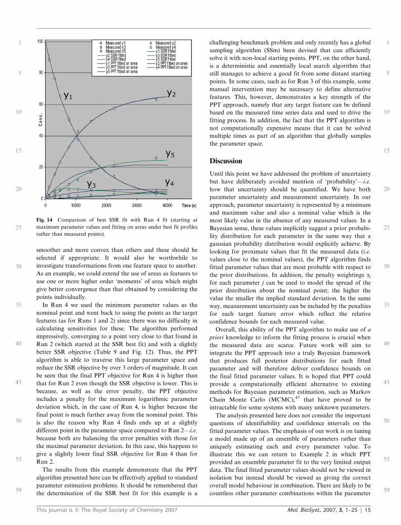
smoother and more convex than others and these should be

selected if appropriate. It would also be worthwhile to

investigate transformations from one feature space to another.

As an example, we could extend the use of areas as features to

use one or more higher order ‘moments’ of area which might

give better convergence than that obtained by considering the

points individually.

In Run 4 we used the minimum parameter values as the

nominal point and went back to using the points as the target

features (as for Runs 1 and 2) since there was no difficulty in

calculating sensitivities for these. The algorithm performed

impressively, converging to a point very close to that found in

Run 2 (which started at the SSR best fit) and with a slightly

better SSR objective (Table 9 and Fig. 12). Thus, the PPT

algorithm is able to traverse this large parameter space and

reduce the SSR objective by over 3 orders of magnitude. It can

be seen that the final PPT objective for Run 4 is higher than

that for Run 2 even though the SSR objective is lower. This is

because, as well as the error penalty, the PPT objective

includes a penalty for the maximum logarithmic parameter

deviation which, in the case of Run 4, is higher because the

final point is much further away from the nominal point. This

is also the reason why Run 4 finds ends up at a slightly

different point in the parameter space compared to Run 2—i.e.

because both are balancing the error penalties with those for

the maximal parameter deviation. In this case, this happens to

give a slightly lower final SSR objective for Run 4 than for

Run 2.

The results from this example demonstrate that the PPT

algorithm presented here can be effectively applied to standard

parameter estimation problems. It should be remembered that

the determination of the SSR best fit for this example is a

challenging benchmark problem and only recently has a global

sampling algorithm (SSm) been devised that can efficiently

solve it with non-local starting points. PPT, on the other hand,

is a deterministic and essentially local search algorithm that

still manages to achieve a good fit from some distant starting

points. In some cases, such as for Run 3 of this example, some

manual intervention may be necessary to define alternative

features. This, however, demonstrates a key strength of the

PPT approach, namely that any target feature can be defined

based on the measured time series data and used to drive the

fitting process. In addition, the fact that the PPT algorithm is

not computationally expensive means that it can be solved

multiple times as part of an algorithm that globally samples

the parameter space.

Discussion

Until this point we have addressed the problem of uncertainty

but have deliberately avoided mention of ‘probability’—i.e.

how that uncertainty should be quantified. We have both

parameter uncertainty and measurement uncertainty. In our

approach, parameter uncertainty is represented by a minimum

and maximum value and also a nominal value which is the

most likely value in the absence of any measured values. In a

Bayesian sense, these values implicitly suggest a prior probabi-

lity distribution for each parameter in the same way that a

gaussian probability distribution would explicitly achieve. By

looking for proximate values that fit the measured data (i.e.

values close to the nominal values), the PPT algorithm finds

fitted parameter values that are most probable with respect to

the prior distributions. In addition, the penalty weightings aj

for each parameter j can be used to model the spread of the

prior distribution about the nominal point; the higher the

value the smaller the implied standard deviation. In the same

way, measurement uncertainty can be included by the penalties

for each target feature error which reflect the relative

confidence bounds for each measured value.

Overall, this ability of the PPT algorithm to make use of a

priori knowledge to inform the fitting process is crucial when

the measured data are scarce. Future work will aim to

integrate the PPT approach into a truly Bayesian framework

that produces full posterior distributions for each fitted

parameter and will therefore deliver confidence bounds on

the final fitted parameter values. It is hoped that PPT could

provide a computationally efficient alternative to existing

methods for Bayesian parameter estimation, such as Markov

Chain Monte Carlo (MCMC),47 that have proved to be

intractable for some systems with many unknown parameters.

The analysis presented here does not consider the important

questions of identifiability and confidence intervals on the

fitted parameter values. The emphasis of our work is on tuning

a model made up of an ensemble of parameters rather than

uniquely estimating each and every parameter value. To

illustrate this we can return to Example 2 in which PPT

provided an ensemble parameter fit to the very limited output

data. The final fitted parameter values should not be viewed in

isolation but instead should be viewed as giving the correct

overall model behaviour in combination. There are likely to be

countless other parameter combinations within the parameter

Fig. 14 Comparison of best SSR fit with Run 4 fit (starting at

maximum parameter values and fitting on areas under best fit profiles

rather than measured points).


1

5

10

15

20

25

30

35

40

45

50

55

59

1

5

10

15

20

25

30

35

40

45

50

55

59

space that give the same fit—possibly some that are closer to

the nominal values since PPT does not guarantee finding the

global optimum. While more data to discriminate them is anti-

cipated, the PPT solution provides a fit to the existing data.

In this paper we offer no theoretical guarantees of

convergence for the PPT algorithm. In fact, as can be seen in

examples 3 or 4, it can exhibit divergent or oscillatory

behaviour in which the size of the steps taken in the parameter

space do not vanish to zero. This has not been a problem for

these examples—we just used a preset number of iterations and

choose the minimum objective of all of them as the final

solution which was good enough. There may, however, be

more pathological systems of ODEs in which LP-PPT fails to

find a reasonable solution at all. Ultimately, the convergence

of the algorithm depends on the accuracy of the linear

approximation that is used by the LP sub-problem to predict

that point in the parameter space that will minimize the

objective function. An analysis of this error for Example 1 is

given in Appendix B. If there are significant higher order terms

and/or strong correlations between parameters then the

discrepancy between the predicted feature errors and the

actual errors at each point in the parameter space may grow to

such an extent that LP-PPT fails. In this case we would need to

reduce the step length or else switch to QP-PPT (Appendix C)

which takes account of second order terms. The error between

predicted and actual errors can be monitored as the algorithm

proceeds and appropriate action can be taken if it gets too high

(switch to QP-PPT, reduce step length etc.)

Despite the potential limitations of LP-PPT caused by its

use of a local linearization at each step, this same approxima-

tion results in a very efficient algorithm in computational

terms since the small linear programming sub-problems can be

solved very quickly. The main computational burden in the

current implementation occurs in Step 4 in which the

sensitivities are estimated numerically therefore requiring at

least one simulation per parameter to be estimated. For the

results reported in this paper we have made no efforts to make

this step more efficient since the longest of our runs took less

than 10 min of CPU time. However, there is certainly scope to

do significantly improve efficiency if, for example, the

algorithm were to be repeatedly solved a part of an intensive

sampling strategy. We use two simulations per parameter since

we estimate the local sensitivity by perturbing each parameter

value upwards and downwards by 0.1% and take the average;

however one perturbation would probably suffice. It may also

be possible to take other short-cuts to reduce the calculation

time. We found that many of the sensitivities do not vary much

from one step to another since the region of feature space is

locally quite flat or the only small steps are being made in the

direction of some parameters. Under these circumstances, the

algorithm could use simple interpolation to approximate

the sensitivities in parameter directions that are only weakly

varying and only perform full updates using perturbed

simulations when necessary. This is analogous to projected

Hessian approximations used in quasi-Newton methods for

nonlinear programming.48

We introduced the PPT algorithm as being applicable for

networks whose structure and kinetics are known with the only

uncertainty residing in the kinetic constants and initial

concentrations. However, PPT can be applied in exactly the

same way to networks in which we do not known the form of

the kinetic equations because we can use lin-log49,50 or other

generalized kinetics51 that can give good approximations over

a wide range. It may also be possible to extend the approach

further problems in which the structure of the biochemical

network is uncertain. In this case, we could postulate a ‘super-

structure’ of all possible interactions and allow the algorithm

to select the smallest subset that best explains the measured

data. To do this exactly would require the solution of a mixed

integer linear programming (MILP) problem in step 5 of the

general PPT algorithm since it requires binary variables to

model the inclusion of each candidate parameter in the fitted

model (see Appendix C). However, we could generate

approximate solutions using the existing LP-PPT implementa-

tion described here. In order to do this the lower bounds on the

rate constant for each uncertain reaction would be set to a

negligible value; small enough to represent the absence of an

interaction (note that we cannot use a lower bound of zero

because the LP-PPT algorithm uses the logarithms of these

quantities). The algorithm would then start from a nominal

point with all rate constants at their minimum values—i.e. the

lower extreme of their ranges rather than at intermediate

values - and, by increasing parameter values, would introduce

the minimal subset of interactions to fit the model to the data.

This would necessitate the use of positive values for the aj

parameters that penalize the inclusion of each parameter j.

This approach has some similarities with the recent work of

Papadopoulos and Brown52 which uses the sum of the

parameter deviations as a proximity metric in order to obtain

‘sparse’ models containing the fewest number of parameters.

A key feature of the LP-PPT algorithm as presented in this

paper is that it is deterministic. For a given starting point and a

pre-set step length, the algorithm will end up at a unique point

in the parameter space after a certain number of iterations.

The only circumstances in which different implementations of

the algorithm might terminate at different end points would be

if there is degeneracy in an LP sub-problem (more than one

solution that gives the optimal objective). In this case different

LP solvers might make different choices about which solution

to select and therefore which direction to step next in the

parameter space. For the LP solver this choice is arbitrary

since all the predicted solutions are equally good but this will

effect the trajectory of the algorithm as a whole is likely to lead

to a different end point. One could easily eliminate this arbitrary

choice by requiring the algorithm to consider all degenerate LP

solutions by performing a simulation at each predicted step in

the parameter space. The algorithm would then select the

predicted point that gave the best actual objective.

In summary the proximate parameter tuning algorithm is a

novel approach for adjusting biochemical models to fit target

output values using prior knowledge about the parameter

values. The algorithm can use any type of output feature and

scales well with the number of output features to be fitted and

the number of uncertain parameters to be adjusted. The

examples presented demonstrate that the algorithm performs

well on a diverse problem set. The approach is deterministic

and is therefore complimentary to those based on random

sampling or evolutionary algorithms.


1

5

10

15

20

25

30

35

40

45

50

55

59

1

5

10

15

20

25

30

35

40

45

50

55

59

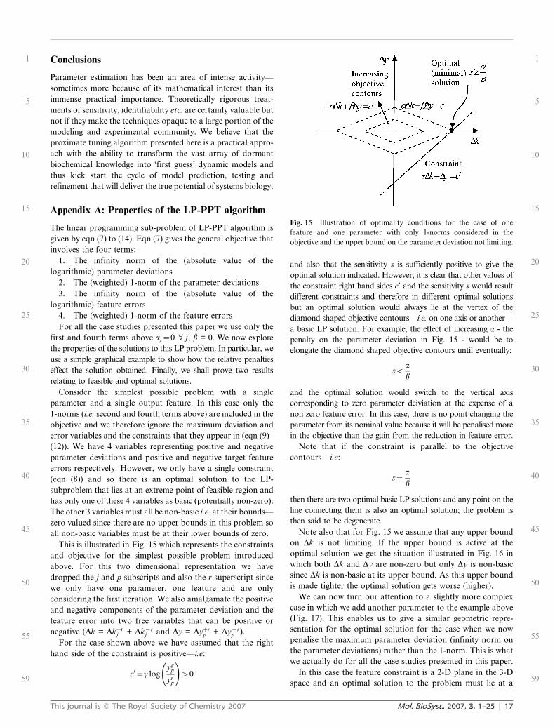
Conclusions

Parameter estimation has been an area of intense activity—

sometimes more because of its mathematical interest than its

immense practical importance. Theoretically rigorous treat-

ments of sensitivity, identifiability etc. are certainly valuable but

not if they make the techniques opaque to a large portion of the

modeling and experimental community. We believe that the

proximate tuning algorithm presented here is a practical appro-

ach with the ability to transform the vast array of dormant

biochemical knowledge into ‘first guess’ dynamic models and

thus kick start the cycle of model prediction, testing and

refinement that will deliver the true potential of systems biology.

Appendix A: Properties of the LP-PPT algorithm

The linear programming sub-problem of LP-PPT algorithm is

given by eqn (7) to (14). Eqn (7) gives the general objective that

involves the four terms:

1. The infinity norm of the (absolute value of the

logarithmic) parameter deviations

2. The (weighted) 1-norm of the parameter deviations

3. The infinity norm of the (absolute value of the

logarithmic) feature errors

4. The (weighted) 1-norm of the feature errors

For all the case studies presented this paper we use only the

first and fourth terms above aj~0 V j, b = 0. We now explore

the properties of the solutions to this LP problem. In particular, we

use a simple graphical example to show how the relative penalties

effect the solution obtained. Finally, we shall prove two results

relating to feasible and optimal solutions.

Consider the simplest possible problem with a single

parameter and a single output feature. In this case only the

1-norms (i.e. second and fourth terms above) are included in the

objective and we therefore ignore the maximum deviation and

error variables and the constraints that they appear in (eqn (9)–

(12)). We have 4 variables representing positive and negative

parameter deviations and positive and negative target feature

errors respectively. However, we only have a single constraint

(eqn (8)) and so there is an optimal solution to the LP-

subproblem that lies at an extreme point of feasible region and

has only one of these 4 variables as basic (potentially non-zero).

The other 3 variables must all be non-basic i.e. at their bounds—

zero valued since there are no upper bounds in this problem so

all non-basic variables must be at their lower bounds of zero.

This is illustrated in Fig. 15 which represents the constraints

and objective for the simplest possible problem introduced

above. For this two dimensional representation we have

dropped the j and p subscripts and also the r superscript since

we only have one parameter, one feature and are only

considering the first iteration. We also amalgamate the positive

and negative components of the parameter deviation and the

feature error into two free variables that can be positive or

negative (Dk = Dkþrj + Dk{r

j and Dy = Dyþrp + Dy{r

p ).

For the case shown above we have assumed that the right

hand side of the constraint is positive—i.e:

c0~c logyg

p

yrp

!w0

and also that the sensitivity s is sufficiently positive to give the

optimal solution indicated. However, it is clear that other values of

the constraint right hand sides c9 and the sensitivity s would result

different constraints and therefore in different optimal solutions

but an optimal solution would always lie at the vertex of the

diamond shaped objective contours—i.e. on one axis or another—

a basic LP solution. For example, the effect of increasing a - the

penalty on the parameter deviation in Fig. 15 - would be to

elongate the diamond shaped objective contours until eventually:

sva

b

and the optimal solution would switch to the vertical axis

corresponding to zero parameter deiviation at the expense of a

non zero feature error. In this case, there is no point changing the

parameter from its nominal value because it will be penalised more

in the objective than the gain from the reduction in feature error.

Note that if the constraint is parallel to the objective

contours—i.e:

s~a

b

then there are two optimal basic LP solutions and any point on the

line connecting them is also an optimal solution; the problem is

then said to be degenerate.

Note also that for Fig. 15 we assume that any upper bound

on Dk is not limiting. If the upper bound is active at the

optimal solution we get the situation illustrated in Fig. 16 in

which both Dk and Dy are non-zero but only Dy is non-basic

since Dk is non-basic at its upper bound. As this upper bound

is made tighter the optimal solution gets worse (higher).

We can now turn our attention to a slightly more complex

case in which we add another parameter to the example above

(Fig. 17). This enables us to give a similar geometric repre-

sentation for the optimal solution for the case when we now

penalise the maximum parameter deviation (infinity norm on

the parameter deviations) rather than the 1-norm. This is what

we actually do for all the case studies presented in this paper.

In this case the feature constraint is a 2-D plane in the 3-D

space and an optimal solution to the problem must lie at a

Fig. 15 Illustration of optimality conditions for the case of one

feature and one parameter with only 1-norms considered in the

objective and the upper bound on the parameter deviation not limiting.


1

5

10

15

20

25

30

35

40

45

50

55

59

1

5

10

15

20

25

30

35

40

45

50

55

59

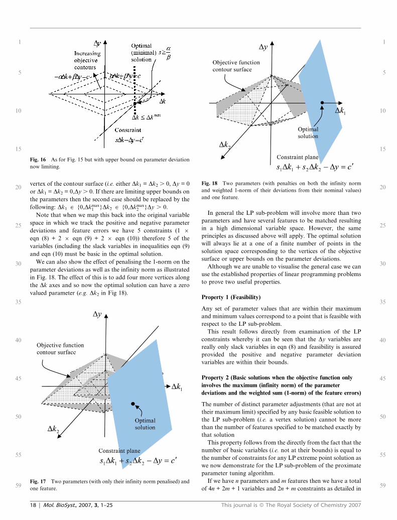
vertex of the contour surface (i.e. either Dk1 = Dk2 . 0, Dy = 0

or Dk1 = Dk2 = 0,Dy . 0. If there are limiting upper bounds on

the parameters then the second case should be replaced by the

following: Dk1 s {0,Dkmax1 }Dk2 s {0,Dkmax

2 }Dy . 0.

Note that when we map this back into the original variable

space in which we track the positive and negative parameter

deviations and feature errors we have 5 constraints (1 6eqn (8) + 2 6 eqn (9) + 2 6 eqn (10)) therefore 5 of the

variables (including the slack variables in inequalities eqn (9)

and eqn (10) must be basic in the optimal solution.

We can also show the effect of penalising the 1-norm on the

parameter deviations as well as the infinity norm as illustrated

in Fig. 18. The effect of this is to add four more vertices along

the Dk axes and so now the optimal solution can have a zero

valued parameter (e.g. Dk2 in Fig 18).

In general the LP sub-problem will involve more than two

parameters and have several features to be matched resulting

in a high dimensional variable space. However, the same

principles as discussed above will apply. The optimal solution

will always lie at a one of a finite number of points in the

solution space corresponding to the vertices of the objective

surface or upper bounds on the parameter deviations.

Although we are unable to visualise the general case we can

use the established properties of linear programming problems

to prove two useful properties.

Property 1 (Feasibility)

Any set of parameter values that are within their maximum

and minimum values correspond to a point that is feasible with

respect to the LP sub-problem.

This result follows directly from examination of the LP

constraints whereby it can be seen that the Dy variables are

really only slack variables in eqn (8) and feasibility is assured

provided the positive and negative parameter deviation

variables are within their bounds.

Property 2 (Basic solutions when the objective function only

involves the maximum (infinity norm) of the parameter

deviations and the weighted sum (1-norm) of the feature errors)

The number of distinct parameter adjustments (that are not at

their maximum limit) specified by any basic feasible solution to

the LP sub-problem (i.e. a vertex solution) cannot be more

than the number of features specified to be matched exactly by

that solution

This property follows from the directly from the fact that the

number of basic variables (i.e. not at their bounds) is equal to

the number of constraints for any LP extreme point solution as

we now demonstrate for the LP sub-problem of the proximate

parameter tuning algorithm.

If we have n parameters and m features then we have a total

of 4n + 2m + 1 variables and 2n + m constraints as detailed in

Fig. 16 As for Fig. 15 but with upper bound on parameter deviation

now limiting.

Fig. 17 Two parameters (with only their infinity norm penalised) and

one feature.

Fig. 18 Two parameters (with penalties on both the infinity norm

and weighted 1-norm of their deviations from their nominal values)

and one feature.


1

5

10

15

20

25

30

35

40

45

50

55

59

1

5

10

15

20

25

30

35

40

45

50

55

59

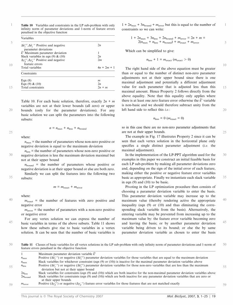
Table 10. For each basic solution, therefore, exactly 2n + m

variables are not at their lower bounds (all zero) or upper

bounds (only for the parameter deviations). For any

basic solution we can split the parameters into the following

subsets:

n = nmax + nless + nbound

where:

nmax = the number of parameters whose non-zero positive or

negative deviation is equal to the maximum deviation

nless = the number of parameters whose non-zero positive or

negative deviation is less the maximum deviation maximal but

not at their upper bound

nbound = the number of parameters whose positive or

negative deviation is at their upper bound or else are both zero.

Similarly we can split the features into the following two

subsets:

m = mexact + merror

where:

mexact = the number of features with zero positive and

negative error

merror = the number of parameters with a non-zero positive

or negative error

For any vertex solution we can express the number of

basic variables in terms of the above subsets. Table 11 shows

how these subsets give rise to basic variables in a vertex

solution. It can be seen that the number of basic variables is

1 + 2nmax + 3nbound + merror but this is equal to the number of

constraints so we can write:

1 + 2nmax + 3nless + 2nbound + merror = 2n + m =2(nmax + nless + nbound) + mexact + merror

Which can be simplified to give:

nless + 1 = mexact (mexact . 0)

The right hand side of the above equation must be greater

than or equal to the number of distinct non-zero parameter

adjustments not at their upper bound since there is one

maximal adjustment and potentially a different adjustment

value for each parameter that is adjusted less than this

maximal amount. Hence Property 2 follows directly from the

above equality. Note that this equality only applies where

there is at least one zero feature error otherwise the kr variable

is non-basic and we should therefore subtract unity from the

left hand side to reflect this i.e.:

nless = 0 (mexact = 0)

so in this case there are no non-zero parameter adjustments that

are not at their upper bounds.

The example in Fig. 17 illustrates Property 2 since it can be

seen that each vertex solution in the horizontal plane only

specifies a single distinct parameter adjustment (i.e. the

maximal adjustment).

In the implementation of the LP-PPT algorithm used for the

examples in this paper we construct an initial feasible basis for

each LP sub-problem by making all parameter deviations zero

and, depending on the sign of the initial error of each feature,

making either the positive or negative feature error variables

basic as appropriate. Finally we instantiate each slack variable

in eqn (9) and (10) to be basic.

Pivoting in the LP optimization procedure then consists of

choosing a parameter deviation variable to enter the basis.

This parameter deviation variable may increase up to the

maximum value (thereby rendering active the appropriate

inequality (eqn (9) or (10) and thus eliminating the corre-

sponding slack variable from the basis). Alternatively, the

entering variable may be prevented from increasing up to the

maximum value by: the feature error variable becoming zero

and leaving the basis; or by another parameter deviation

variable being driven to its bound; or else the by same

parameter deviation variable as chosen to enter the basis

Table 10 Variables and constraints in the LP sub-problem with onlyinfinity norm of parameter deviations and 1-norm of feature errorspenalised in the objective function

Variables

Dkþrj ,Dk{r

j Positive and negative

parameter deviations

2n

kr Maximum parameter deviation 1Slack variables in eqn (9) & (10) 2nDyþr

p ,Dy{rp Positive and negative

feature errors

2m

Total variables 4n + 2m + 1

Constraints

Eqn (8) mEqn (9) & (10) 2nTotal constraints 2n + m

Table 11 Classes of basic variables for all vertex solutions in the LP sub-problem with only infinity norm of parameter deviations and 1-norm offeature errors penalised in the objective function

1 Maximum parameter deviation variable kr

nmax Positive (Dk{rj ) or negative (Dkþr

j ) parameter deviation variables for those variables that are equal to the maximum deviation

nmax Slack variables for whichever constraint (eqn (9) or (10)) is inactive for the maximal parameter deviation variables abovenless Positive (Dk{r

j ) or negative (Dkþrj ) parameter deviation variables for those non-zero variables that are less than the maximum

deviation but not at their upper bound2nless Slack variables for constraints (eqn (9) and (10)) which are both inactive for the non-maximal parameter deviation variables above2nbound Slack variables for constraints (eqn (9) and (10)) which are both inactive for any parameter deviation variables that are zero or

at their upper boundsmerror Positive (Dyþr

p ) or negative (Dy{rp ) feature error variables for those features that are not matched exactly


1

5

10

15

20

25

30

35

40

45

50

55

59

1

5

10

15

20

25

30

35

40

45

50

55

59

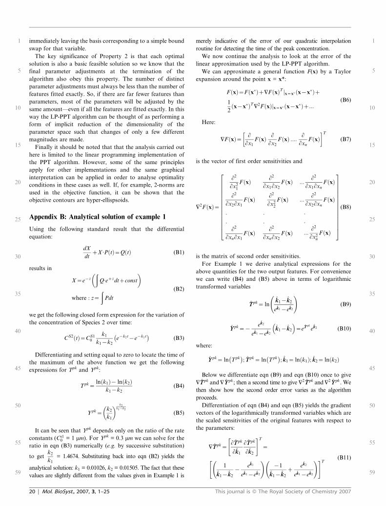
immediately leaving the basis corresponding to a simple bound

swap for that variable.

The key significance of Property 2 is that each optimal

solution is also a basic feasible solution so we know that the

final parameter adjustments at the termination of the

algorithm also obey this property. The number of distinct

parameter adjustments must always be less than the number of

features fitted exactly. So, if there are far fewer features than

parameters, most of the parameters will be adjusted by the

same amount—even if all the features are fitted exactly. In this

way the LP-PPT algorithm can be thought of as performing a

form of implicit reduction of the dimensionality of the

parameter space such that changes of only a few different

magnitudes are made.

Finally it should be noted that that the analysis carried out

here is limited to the linear programming implementation of

the PPT algorithm. However, some of the same principles

apply for other implementations and the same graphical

interpretation can be applied in order to analyse optimality

conditions in these cases as well. If, for example, 2-norms are

used in the objective function, it can be shown that the

objective contours are hyper-ellispsoids.

Appendix B: Analytical solution of example 1

Using the following standard result that the differential

equation:

dX

dtzX :P tð Þ~Q tð Þ (B1)

results in

X~e{z

ðQ:ezzdtzconst

� �

where : z~

ðPdt

(B2)

we get the following closed form expression for the variation of

the concentration of Species 2 over time:

CS2 tð Þ~CS10

k1

k1{k2e{k2t{e{k1t� �

(B3)

Differentiating and setting equal to zero to locate the time of

the maximum of the above function we get the following

expressions for Tpk and Ypk:

Tpk~ln k1ð Þ{ ln k2ð Þ

k1{k2(B4)

Y pk~k2

k1

� � k2k1{k2

(B5)

It can be seen that Ypk depends only on the ratio of the rate

constants (Cs10 = 1 mm). For Ypk = 0.3 mm we can solve for the

ratio in eqn (B3) numerically (e.g. by successive substitution)

to getk2

k1= 1.4674. Substituting back into eqn (B2) yields the

analytical solution: k1 = 0.01026, k2 = 0.01505. The fact that these

values are slightly different from the values given in Example 1 is

merely indicative of the error of our quadratic interpolation

routine for detecting the time of the peak concentration.

We now continue the analysis to look at the error of the

linear approximation used by the LP-PPT algorithm.

We can approximate a general function F(x) by a Taylor

expansion around the point x = x*:

F xð Þ~F x�ð Þz+F xð ÞT x~x�j x{x�ð Þz1

2x{x�ð ÞT+2F xð Þ x~x�j x{x�ð Þz:::

(B6)

Here:

+F xð Þ~ LLx1

F xð Þ LLx2

F xð Þ :::: LLxn

F xð Þ� T

(B7)

is the vector of first order sensitivities and

+2F xð Þ~

L2

Lx21

F xð Þ L2

Lx1Lx2F xð Þ :::

L2

Lx1Lxn

F xð Þ

L2

Lx2Lx1

F xð Þ L2

Lx22

F xð Þ :::L2

Lx2Lxn

F xð Þ

:

:

L2

LxnLx1F xð Þ

:

:

L2

LxnLx2F xð Þ

:

:

:::L2

Lx2n

F xð Þ

266666666666664

377777777777775

(B8)

is the matrix of second order sensitivities.

For Example 1 we derive analytical expressions for the

above quantities for the two output features. For convenience

we can write (B4) and (B5) above in terms of logarithmic

transformed variables

TTpk~ lnkk1{kk2

ekk1{ekk2

!(B9)

YY pk~{ekk2

ekk1{ekk2

kk1{kk2

� �~eTTpk

ekk2 (B10)

where:

YY pk~ ln Tpk� �

; TTpk~ ln Tpk� �

; kk1~ ln k1ð Þ; kk2~ ln k2ð Þ

Below we differentiate eqn (B9) and eqn (B10) once to give

+TTpk and +YY pk; then a second time to give +2TTpk and +2YY pk. We

then show how the second order error varies as the algorithm

proceeds.

Differentiation of eqn (B4) and eqn (B5) yields the gradient

vectors of the logarithmically transformed variables which are

the scaled sensitivities of the original features with respect to

the parameters:

+TTpk~LTTpk

Lkk1

LTTpk

Lkk2

" #T

~

1

kk1{kk2

{ekk1

ekk1{ekk2

!{1

kk1{kk2

zekk2

ekk1{ekk2

!" #T(B11)


1

5

10

15

20

25

30

35

40

45

50

55

59

1

5

10

15

20

25

30

35

40

45

50

55

59

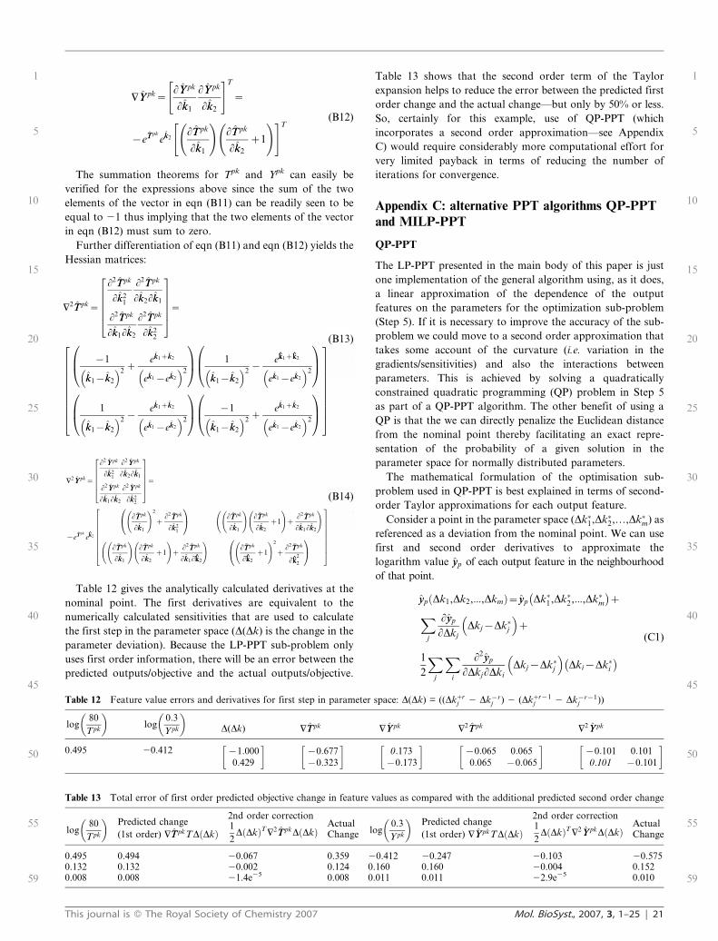
+YY pk~LYY pk

Lkk1

LYY pk

Lkk2

" #T

~

{eTTpk

ekk2LTTpk

Lkk1

!LTTpk

Lkk2

z1

!" #T(B12)

The summation theorems for Tpk and Ypk can easily be

verified for the expressions above since the sum of the two

elements of the vector in eqn (B11) can be readily seen to be

equal to 21 thus implying that the two elements of the vector

in eqn (B12) must sum to zero.

Further differentiation of eqn (B11) and eqn (B12) yields the

Hessian matrices:

+2TTpk~

L2TTpk

Lkk21

L2TTpk

Lkk2Lkk1

L2TTpk

Lkk1Lkk2

L2TTpk

Lkk22

266664

377775~

{1

kk1{kk2

� �2z

ekk1zkk2

ekk1 {ekk2

� �2

0B@

1CA

1

kk1{kk2

� �2{

ekk1zkk2

ekk1 {ekk2

� �2

0B@

1CA

1

kk1{kk2

� �2{

ekk1zkk2

ekk1 {ekk2

� �2

0B@

1CA

{1

kk1{kk2

� �2z

ekk1zkk2

ekk1 {ekk2

� �2

0B@

1CA

26666666664

37777777775

(B13)

+2YY pk~

L2YY pk

Lkk21

L2YY pk

Lkk2Lkk1

L2YY pk

Lkk1Lkk2

L2YY pk

Lkk22

2

66664

3

77775~

{eTTpk

ekk2

LTTpk

Lkk1

!2

zL2TTpk

Lkk21

0@

1A LTTpk

Lkk1

!LTTpk

Lkk2

z1

!z

L2TTpk

Lkk1Lkk2

!

LTTpk

Lkk1

!LTTpk

Lkk2

z1

!z

L2TTpk

Lkk1Lkk2

!LTTpk

Lkk2

z1

!2

zL2TTpk

Lkk2

2

0@

1A

266666664

377777775

(B14)

Table 12 gives the analytically calculated derivatives at the

nominal point. The first derivatives are equivalent to the

numerically calculated sensitivities that are used to calculate

the first step in the parameter space (D(Dk) is the change in the

parameter deviation). Because the LP-PPT sub-problem only

uses first order information, there will be an error between the

predicted outputs/objective and the actual outputs/objective.

Table 13 shows that the second order term of the Taylor

expansion helps to reduce the error between the predicted first

order change and the actual change—but only by 50% or less.

So, certainly for this example, use of QP-PPT (which

incorporates a second order approximation—see Appendix

C) would require considerably more computational effort for

very limited payback in terms of reducing the number of

iterations for convergence.

Appendix C: alternative PPT algorithms QP-PPT

and MILP-PPT

QP-PPT

The LP-PPT presented in the main body of this paper is just

one implementation of the general algorithm using, as it does,

a linear approximation of the dependence of the output

features on the parameters for the optimization sub-problem

(Step 5). If it is necessary to improve the accuracy of the sub-

problem we could move to a second order approximation that

takes some account of the curvature (i.e. variation in the

gradients/sensitivities) and also the interactions between

parameters. This is achieved by solving a quadratically

constrained quadratic programming (QP) problem in Step 5

as part of a QP-PPT algorithm. The other benefit of using a

QP is that the we can directly penalize the Euclidean distance

from the nominal point thereby facilitating an exact repre-

sentation of the probability of a given solution in the

parameter space for normally distributed parameters.

The mathematical formulation of the optimisation sub-

problem used in QP-PPT is best explained in terms of second-

order Taylor approximations for each output feature.

Consider a point in the parameter space (Dk�1,Dk�2,…,Dk�m) as

referenced as a deviation from the nominal point. We can use

first and second order derivatives to approximate the

logarithm value yyp of each output feature in the neighbourhood

of that point.

yyp Dk1,Dk2,:::,Dkmð Þ~yyp Dk�1,Dk�2,:::,Dk�m� �

z

X

j

Lyyp

LDkj

Dkj{Dk�j

� �z

1

2

X

j

X

i

L2yyp

LDkjLDki

Dkj{Dk�j

� �Dki{Dk�i� �

(C1)

(B13)

Table 12 Feature value errors and derivatives for first step in parameter space: D(Dk) = ((Dkþrj 2 Dk{r

j ) 2 (Dkþr{1j 2 Dk{r{1

j ))

log80

Tpk

� �log

0:3

Y pk

� �

D(Dk) +TTpk +YY pk +2TTpk +2YY pk

0.495 20.412 {1:000

0:429

� {0:677

{0:323

� 0:173

{0:173

� {0:065 0:065

0:065 {0:065

� {0:101 0:101

0:101 {0:101

�

(B14)

Table 13 Total error of first order predicted objective change in feature values as compared with the additional predicted second order change

log80

Tpk

� �Predicted change

(1st order) +TTpkTD Dkð Þ

2nd order correction1

2D Dkð ÞT +2TTpkD Dkð Þ

ActualChange log

0:3

Y pk

� �Predicted change

(1st order) +YY pkTD Dkð Þ

2nd order correction1

2D Dkð ÞT +2YY pkD Dkð Þ

ActualChange

0.495 0.494 20.067 0.359 20.412 20.247 20.103 20.5750.132 0.132 20.002 0.124 0.160 0.160 20.004 0.1520.008 0.008 21.4e25 0.008 0.011 0.011 22.9e25 0.010


1

5

10

15

20

25

30

35

40

45

50

55

59

1

5

10

15

20

25

30

35

40

45

50

55

59

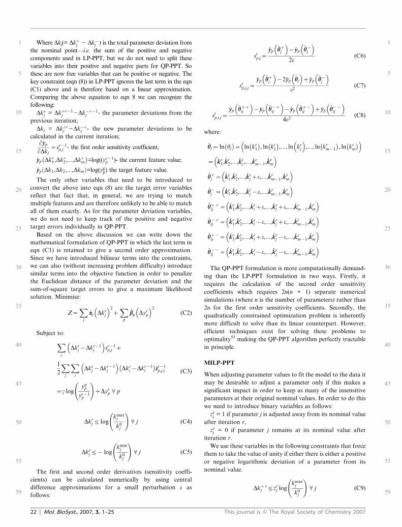
Where Dkj(= Dkþj 2 Dk{j ) is the total parameter deviation from

the nominal point—i.e. the sum of the positive and negative

components used in LP-PPT, but we do not need to split these

variables into their positive and negative parts for QP-PPT. So

these are now free variables that can be positive or negative. The

key constraint (eqn (8)) in LP-PPT ignores the last term in the eqn

(C1) above and is therefore based on a linear approximation.

Comparing the above equation to eqn 8 we can recognize the

following:

Dk�j = Dkþr{1j 2Dk{r{1

j - the parameter deviations from the

previous iteration;

Dkj = Dkþrj 2Dk{r

j - the new parameter deviations to be

calculated in the current iteration;Lyyp

LDkj

~sr{1p,j - the first order sensitivity coefficient;

yyp Dk�1,Dk�2,:::,Dk�m� �

=log((yr{1p )- the current feature value;

yyp Dk1,Dk2,:::,Dkmð Þ=log(ygp) the target feature value.

The only other variables that need to be introduced to

convert the above into eqn (8) are the target error variables

reflect that fact that, in general, we are trying to match

multiple features and are therefore unlikely to be able to match

all of them exactly. As for the parameter deviation variables,

we do not need to keep track of the positive and negative

target errors individually in QP-PPT.

Based on the above discussion we can write down the

mathematical formulation of QP-PPT in which the last term in

eqn (C1) is retained to give a second order approximation.

Since we have introduced bilinear terms into the constraints,

we can also (without increasing problem difficulty) introduce

similar terms into the objective function in order to penalize

the Euclidean distance of the parameter deviation and the

sum-of-square target errors to give a maximum likelihood

solution. Minimise:

Z~X

j

aaj Dkrj

� �2

zX

p

bbp Dyrp

� �2

(C2)

Subject to:

X

j

Dkrj {Dkr{1

j

� �sr{1

p,j z

1

2

X

j

X

i

Dkrj {Dkr{1

j

� �Dkr

i {Dkr{1i

� �ssr{1

p,j,i

~c logyg

p

yr{1p

!zDyr

p V p

(C3)

Dkrj ƒ log

kmaxj

k0j

!V j (C4)

Dkrj ƒ{ log

kminj

k0j

!V j (C5)

The first and second order derivatives (sensitivity coeffi-

cients) can be calculated numerically by using central

difference approximations for a small perturbation e as

follows:

srp,j~

yyp hhzj

� �{yyp hh{

j

� �

2e(C6)

srp,j,j~

yyp hhzj

� �{2yyp hhj

� �zyyp hh{

j

� �

e2(C7)

srp,i,j~

yyp hhzzij

� �{yyp hh{z

ij

� �{yyp hhz{

ij

� �zyyp hh{{

ij

� �

4e2(C8)

where:

hhj~ ln hj

� �~ ln kr

1

� �, ln kr

1

� �,:::, ln kr

j

� �,:::, ln kr

m{1

� �, ln kr

m

� ��

~ kkr1,kkr

2,:::,kkrj ,:::,kk

rm{1,kkr

m

� �

hhzj ~ kkr

1,kkr2,:::,kkr

j ze,:::,kkrm{1,kkr

m

� �

hh{j ~ kkr

1,kkr2,:::,kkr

j {e,:::,kkrm{1,kkr

m

� �

hhzzij ~ kkr

1,kkr2,:::,kkr

i ze,:::,kkrj ze,:::,kkr

m{1,kkrm

� �

hh{zij ~ kkr

1,kkr2,:::,kkr

i {e,:::,kkrj ze,:::,kkr

m{1,kkrm

� �

hhz{ij ~ kkr

1,kkr2,:::,kkr

i ze,:::,kkrj {e,:::,kkr

m{1,kkrm

� �

hh{{ij ~ kkr

1,kkr2,:::,kkr

i {e,:::,kkrj {e,:::,kkr

m{1,kkrm

� �

The QP-PPT formulation is more computationally demand-

ing than the LP-PPT formulation in two ways. Firstly, it

requires the calculation of the second order sensitivity

coefficients which requires 2n(n + 1) separate numerical

simulations (where n is the number of parameters) rather than

2n for the first order sensitivity coefficients. Secondly, the

quadratically constrained optimization problem is inherently

more difficult to solve than its linear counterpart. However,

efficient techniques exist for solving these problems to

optimality53 making the QP-PPT algorithm perfectly tractable

in principle.

MILP-PPT

When adjusting parameter values to fit the model to the data it

may be desirable to adjust a parameter only if this makes a

significant impact in order to keep as many of the insensitive

parameters at their original nominal values. In order to do this

we need to introduce binary variables as follows:

zrj = 1 if parameter j is adjusted away from its nominal value

after iteration r,

zrj = 0 if parameter j remains at its nominal value after

iteration r.

We use these variables in the following constraints that force

them to take the value of unity if either there is either a positive

or negative logarithmic deviation of a parameter from its

nominal value.

Dkzj

rƒzr

j logkmax

j

k0j

!V j (C9)


1

5

10

15

20

25

30

35

40

45

50

55

59

1

5

10

15

20

25

30

35

40

45

50

55

59

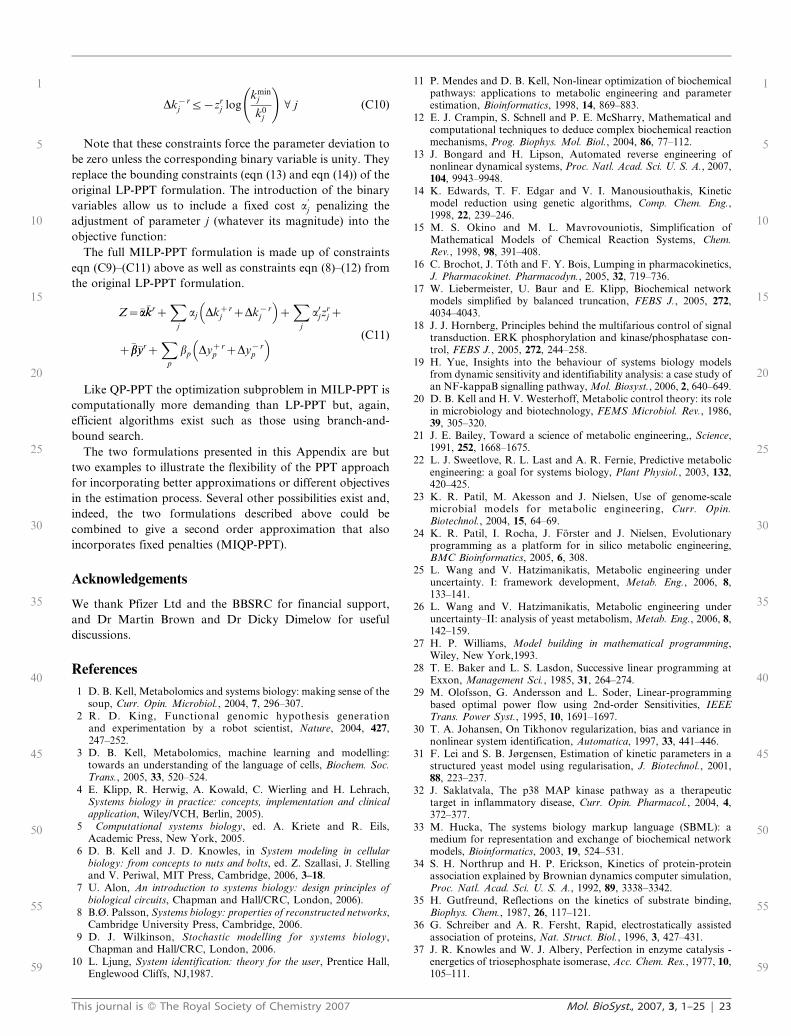
Dk{j

rƒ{zr

j logkmin

j

k0j

!V j (C10)

Note that these constraints force the parameter deviation to

be zero unless the corresponding binary variable is unity. They

replace the bounding constraints (eqn (13) and eqn (14)) of the

original LP-PPT formulation. The introduction of the binary

variables allow us to include a fixed cost a9j penalizing the

adjustment of parameter j (whatever its magnitude) into the

objective function:

The full MILP-PPT formulation is made up of constraints

eqn (C9)–(C11) above as well as constraints eqn (8)–(12) from

the original LP-PPT formulation.

Z~�aa�kkrzX

j

aj Dkzj

rzDk{j

r� �

zX

j

a0jzrj z

z�bb�yyrzX

p

bp Dyzp

rzDy{p

r� � (C11)

Like QP-PPT the optimization subproblem in MILP-PPT is

computationally more demanding than LP-PPT but, again,

efficient algorithms exist such as those using branch-and-

bound search.

The two formulations presented in this Appendix are but

two examples to illustrate the flexibility of the PPT approach

for incorporating better approximations or different objectives

in the estimation process. Several other possibilities exist and,

indeed, the two formulations described above could be

combined to give a second order approximation that also

incorporates fixed penalties (MIQP-PPT).

Acknowledgements

We thank Pfizer Ltd and the BBSRC for financial support,

and Dr Martin Brown and Dr Dicky Dimelow for useful

discussions.

References

1 D. B. Kell, Metabolomics and systems biology: making sense of thesoup, Curr. Opin. Microbiol., 2004, 7, 296–307.

2 R. D. King, Functional genomic hypothesis generationand experimentation by a robot scientist, Nature, 2004, 427,247–252.

3 D. B. Kell, Metabolomics, machine learning and modelling:towards an understanding of the language of cells, Biochem. Soc.Trans., 2005, 33, 520–524.

4 E. Klipp, R. Herwig, A. Kowald, C. Wierling and H. Lehrach,Systems biology in practice: concepts, implementation and clinicalapplication, Wiley/VCH, Berlin, 2005).

5 Computational systems biology, ed. A. Kriete and R. Eils,Academic Press, New York, 2005.

6 D. B. Kell and J. D. Knowles, in System modeling in cellularbiology: from concepts to nuts and bolts, ed. Z. Szallasi, J. Stellingand V. Periwal, MIT Press, Cambridge, 2006, 3–18.

7 U. Alon, An introduction to systems biology: design principles ofbiological circuits, Chapman and Hall/CRC, London, 2006).

8 B.Ø. Palsson, Systems biology: properties of reconstructed networks,Cambridge University Press, Cambridge, 2006.

9 D. J. Wilkinson, Stochastic modelling for systems biology,Chapman and Hall/CRC, London, 2006.

10 L. Ljung, System identification: theory for the user, Prentice Hall,Englewood Cliffs, NJ,1987.

11 P. Mendes and D. B. Kell, Non-linear optimization of biochemicalpathways: applications to metabolic engineering and parameterestimation, Bioinformatics, 1998, 14, 869–883.

12 E. J. Crampin, S. Schnell and P. E. McSharry, Mathematical andcomputational techniques to deduce complex biochemical reactionmechanisms, Prog. Biophys. Mol. Biol., 2004, 86, 77–112.

13 J. Bongard and H. Lipson, Automated reverse engineering ofnonlinear dynamical systems, Proc. Natl. Acad. Sci. U. S. A., 2007,104, 9943–9948.

14 K. Edwards, T. F. Edgar and V. I. Manousiouthakis, Kineticmodel reduction using genetic algorithms, Comp. Chem. Eng.,1998, 22, 239–246.

15 M. S. Okino and M. L. Mavrovouniotis, Simplification ofMathematical Models of Chemical Reaction Systems, Chem.Rev., 1998, 98, 391–408.

16 C. Brochot, J. Toth and F. Y. Bois, Lumping in pharmacokinetics,J. Pharmacokinet. Pharmacodyn., 2005, 32, 719–736.

17 W. Liebermeister, U. Baur and E. Klipp, Biochemical networkmodels simplified by balanced truncation, FEBS J., 2005, 272,4034–4043.

18 J. J. Hornberg, Principles behind the multifarious control of signaltransduction. ERK phosphorylation and kinase/phosphatase con-trol, FEBS J., 2005, 272, 244–258.

19 H. Yue, Insights into the behaviour of systems biology modelsfrom dynamic sensitivity and identifiability analysis: a case study ofan NF-kappaB signalling pathway, Mol. Biosyst., 2006, 2, 640–649.

20 D. B. Kell and H. V. Westerhoff, Metabolic control theory: its rolein microbiology and biotechnology, FEMS Microbiol. Rev., 1986,39, 305–320.

21 J. E. Bailey, Toward a science of metabolic engineering,, Science,1991, 252, 1668–1675.

22 L. J. Sweetlove, R. L. Last and A. R. Fernie, Predictive metabolicengineering: a goal for systems biology, Plant Physiol., 2003, 132,420–425.

23 K. R. Patil, M. Akesson and J. Nielsen, Use of genome-scalemicrobial models for metabolic engineering, Curr. Opin.Biotechnol., 2004, 15, 64–69.

24 K. R. Patil, I. Rocha, J. Forster and J. Nielsen, Evolutionaryprogramming as a platform for in silico metabolic engineering,BMC Bioinformatics, 2005, 6, 308.

25 L. Wang and V. Hatzimanikatis, Metabolic engineering underuncertainty. I: framework development, Metab. Eng., 2006, 8,133–141.

26 L. Wang and V. Hatzimanikatis, Metabolic engineering underuncertainty–II: analysis of yeast metabolism, Metab. Eng., 2006, 8,142–159.

27 H. P. Williams, Model building in mathematical programming,Wiley, New York,1993.

28 T. E. Baker and L. S. Lasdon, Successive linear programming atExxon, Management Sci., 1985, 31, 264–274.

29 M. Olofsson, G. Andersson and L. Soder, Linear-programmingbased optimal power flow using 2nd-order Sensitivities, IEEETrans. Power Syst., 1995, 10, 1691–1697.

30 T. A. Johansen, On Tikhonov regularization, bias and variance innonlinear system identification, Automatica, 1997, 33, 441–446.

31 F. Lei and S. B. Jørgensen, Estimation of kinetic parameters in astructured yeast model using regularisation, J. Biotechnol., 2001,88, 223–237.

32 J. Saklatvala, The p38 MAP kinase pathway as a therapeutictarget in inflammatory disease, Curr. Opin. Pharmacol., 2004, 4,372–377.

33 M. Hucka, The systems biology markup language (SBML): amedium for representation and exchange of biochemical networkmodels, Bioinformatics, 2003, 19, 524–531.

34 S. H. Northrup and H. P. Erickson, Kinetics of protein-proteinassociation explained by Brownian dynamics computer simulation,Proc. Natl. Acad. Sci. U. S. A., 1992, 89, 3338–3342.

35 H. Gutfreund, Reflections on the kinetics of substrate binding,Biophys. Chem., 1987, 26, 117–121.

36 G. Schreiber and A. R. Fersht, Rapid, electrostatically assistedassociation of proteins, Nat. Struct. Biol., 1996, 3, 427–431.

37 J. R. Knowles and W. J. Albery, Perfection in enzyme catalysis -energetics of triosephosphate isomerase, Acc. Chem. Res., 1977, 10,105–111.


1

5

10

15

20

25

30

35

40

45

50

55

59

1

5

10

15

20

25

30

35

40

45

50

55

59

38 A. Fersht, Structure and mechanism in protein science : a guide toenzyme catalysis and protein folding, W. H. Freeman, SanFrancisco, 1999.

39 B. Schoeberl, C. Eichler-Jonsson, E. D. Gilles and G. Muller,Computational modeling of the dynamics of the MAP kinasecascade activated by surface and internalized EGF receptors, Nat.Biotechnol., 2002, 20, 370–375.

40 B. Teusink, Can yeast glycolysis be understood in terms of in vitrokinetics of the constituent enzymes? Testing biochemistry, Eur. J.Biochem., 2000, 267, 5313–5329.

41 L. Pritchard and D. B. Kell, Schemes of flux control in a model ofSaccharomyces cerevisiae glycolysis, Eur. J. Biochem., 2002, 269,3894–3904.

42 S. Hoops, COPASI: a COmplex PAthway SImulator,Bioinformatics, 2006, 22, 3067–3074.

43 R. Fuguitt and J. E. Hawkins, Rate of thermal isomerization ofa-pinene in the liquid phase, J. Am. Chem. Soc., 1947, 69, 461.

44 G. E. P. Box, W. G. Hunter, J. F. MacGregor and J. Erjavec, Someproblems associated with the analysis of multiresponse data,Technometrics, 1973, 15, 33–51.

45 I. B. Tjoa and L. T. Biegler, Simultaneous solution and optimiza-tion strategies for parameter estimation of differential algebraicequation systems, Ind. Eng. Chem. Res., 1991, 30, 376–385.

46 M. Rodriguez-Fernandez, P. Mendes and J. R. Banga, A hybridapproach for efficient and robust parameter estimation inbiochemical pathways, Biosystems, 2006, 83, 248–265.

47 W. R. Gilks, S. Richardson and D. J. Spiegelhalter, Markov chainMonte Carlo in practice, Chapman and Hall, London, 1996.

48 S. J. Wright, Convergence of projected Hessian approximations inquasi-Newton methods for the nonlinear programming problem,IMA J. Numer. Anal., 1986, 6, 463–474.

49 L. Wu, W. Wang, W. A. van Winden, W. M. van Gulik andJ. J. Heijnen, A new framework for the estimation of controlparameters in metabolic pathways using lin-log kinetics, Eur. J.Biochem., 2004, 271, 3348–3359.

50 M. T. A. P. Kresnowati, W. A. van Winden and J. J. Heijnen,Determination of elasticities, concentration and flux controlcoefficients from transient metabolite data using linlog kinetics,Metabol. Eng., 2005, 7, 142–153.

51 M. Savageau, Biochemical systems analysis: a study of function anddesign in molecular biology, Addison-Wesley, Reading, MA,1976.

52 G. Papadopoulos and M. Brown, Feature sensitivity of bio-chemical signalling pathways, IEEE Symp. Comp. Intell. Bioinf.Comput. Biol., 2007, >in press.

53 S. Boyd and L. Vandenberghe, Convex optimization, CambridgeUniversity Press, Cambridge, 2004.


1

5

10

15

20

25

30

35

40

45

50

55

59

1

5

10

15

20

25

30

35

40

45

50

55

59

Authors Queries

Journal: Molecular BioSystems

Paper: b707506e

Title: Proximate parameter tuning for biochemical networks with uncertain kinetic parameters

Editor’s queries are marked like this... U, and for your convenience line numbers are indicated like this... 5.

Query

Reference

Query Remarks

1 Please provide the remainder of the telephone

number for author affiliation a.

2 For your information: You can cite this article before

you receive notification of the page numbers by

using the following format: Mol. BioSyst., 2007, DOI:

10.1039/b707596e.

3 Please supply units for the values in Table 6.

4 Ref. 52: Can this reference be updated yet? Please

supply details to allow readers to access the

reference (for references where page numbers are

not yet known, please supply the DOI).


1

5

10

15

20

25

30

35

40

45

50

55

59

1

5

10

15

20

25

30

35

40

45

50

55

59

Molecular BioSystems b707506e - dbkgroup.orgdbkgroup.org/Papers/wilkinson_mbs_ppt08.pdf ·...

Documents

Transcript of Molecular BioSystems b707506e - dbkgroup.orgdbkgroup.org/Papers/wilkinson_mbs_ppt08.pdf ·...