Mohammad Ali Jinnah- A Numerical Study of Shock Reflection Phenomena in Shock/Turbulence Interaction
9
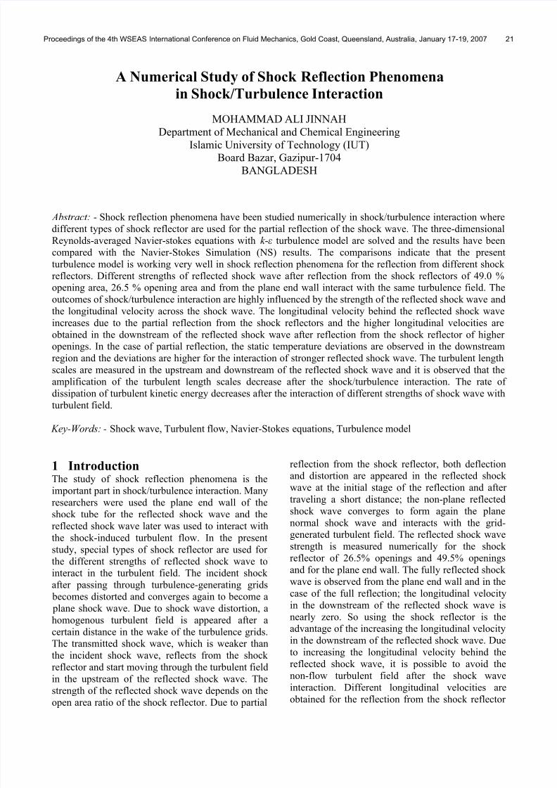
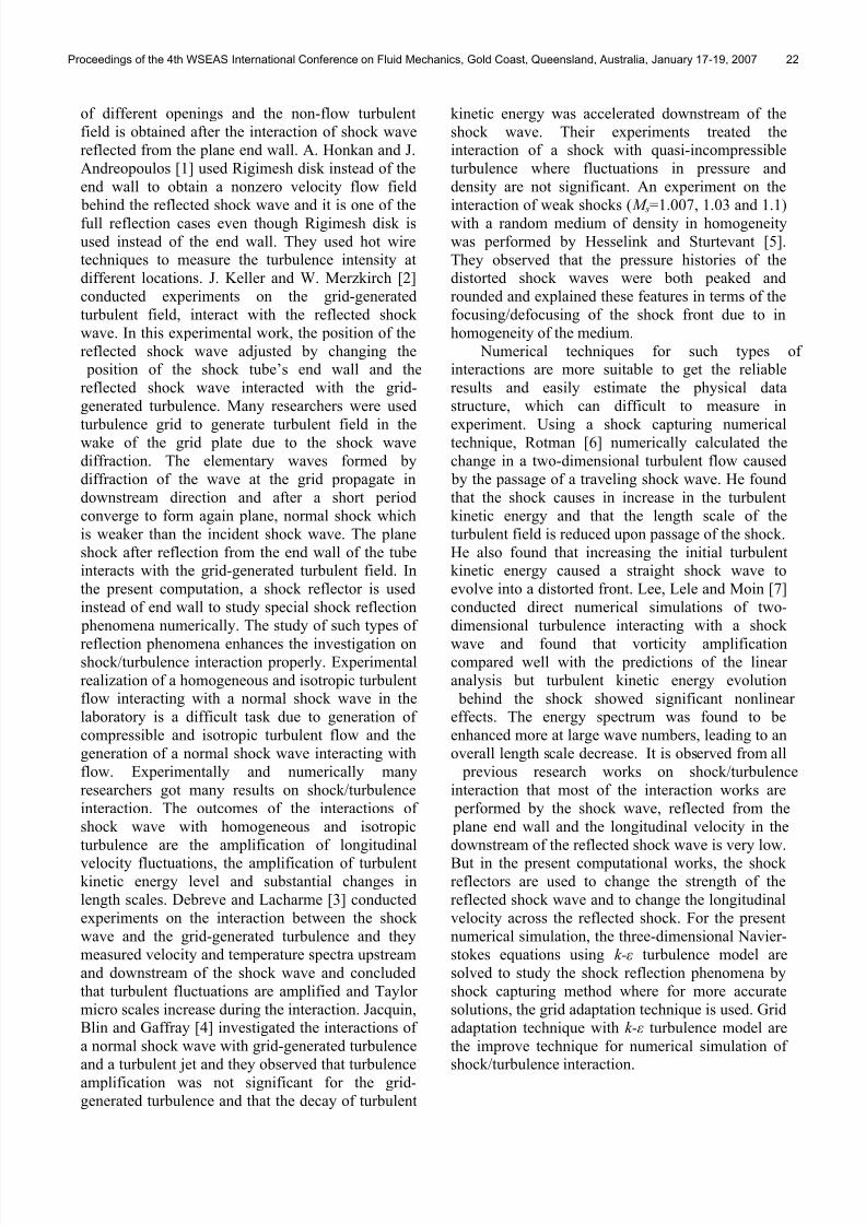
A Numerical Study of Shock Reflection Phenomena in Shock/Turbulence Interaction MOHAMMAD ALI JINNAH Department of Mechanical and Chemical Engineering Islamic University of Technology (IUT) Board Bazar, Gazipur-1704 BANGLADESH Abstract: - Shock reflection phenomena have been studied numerically in shock/turbulence interaction where different types of shock reflector are used for the partial reflection of the shock wave. The three-dimensional Reynolds-averaged Navier-stokes equations with k-ε turbulence model are solved and the results have been compared with the Navier-Stokes Simulation (NS) results. The comparisons indicate that the present turbulence model is working very well in shock reflection phenomena for the reflection from different shock reflectors. Different strengths of reflected shock wave after reflection from the shock reflectors of 49.0 % opening area, 26.5 % opening area and from the plane end wall interact with the same turbulence field. The outcomes of shock/turbulence interaction are highly influenced by the strength of the reflected shock wave and the longitudinal velocity across the shock wave. The longitudinal velocity behind the reflected shock wave increases due to the partial reflection from the shock reflectors and the higher longitudinal velocities are obtained in the downstream of the reflected shock wave after reflection from the shock reflector of higher openings. In the case of partial reflection, the static temperature deviations are observed in the downstream region and the deviations are higher for the interaction of stronger reflected shock wave. The turbulent length scales are measured in the upstream and downstream of the reflected shock wave and it is observed that the amplification of the turbulent length scales decrease after the shock/turbulence interaction. The rate of dissipation of turbulent kinetic energy decreases after the interaction of different strengths of shock wave with turbulent field. Key-Words: - Shock wave, Turbulent flow, Navier-Stokes equations, Turbulence model 1 Introduction The study of shock reflection phenomena is the important part in shock/turbulence interaction. Many researchers were used the plane end wall of the shock tube for the reflected shock wave and the reflected shock wave later was used to interact with the shock-induced turbulent flow. In the present study, special types of shock reflector are used for the different strengths of reflected shock wave to interact in the turbulent field. The incident shock after passing through turbulence-generating grids becomes distorted and converges again to become a plane shock wave. Due to shock wave distortion, a homogenous turbulent field is appeared after a certain distance in the wake of the turbulence grids. The transmitted shock wave, which is weaker than the incident shock wave, reflects from the shock reflector and start moving through the turbulent field in the upstream of the reflected shock wave. The strength of the reflected shock wave depends on the open area ratio of the shock reflector. Due to partial reflection from the shock reflector, both deflection and distortion are appeared in the reflected shock wave at the initial stage of the reflection and after traveling a short distance; the non-plane reflected shock wave converges to form again the plane normal shock wave and interacts with the grid- generated turbulent field. The reflected shock wave strength is measured numerically for the shock reflector of 26.5% openings and 49.5% openings and for the plane end wall. The fully reflected shock wave is observed from the plane end wall and in the case of the full reflection; the longitudinal velocity in the downstream of the reflected shock wave is nearly zero. So using the shock reflector is the advantage of the increasing the longitudinal velocity in the downstream of the reflected shock wave. Due to increasing the longitudinal velocity behind the reflected shock wave, it is possible to avoid the non-flow turbulent field after the shock wave interaction. Different longitudinal velocities are obtained for the reflection from the shock reflector Proceedings of the 4th WSEAS International Conference on Fluid Mechanics, Gold Coast, Queensland, Australia, January 17-19, 2007 21
-
Upload
whitelighte -
Category
Documents
-
view
222 -
download
0
Transcript of Mohammad Ali Jinnah- A Numerical Study of Shock Reflection Phenomena in Shock/Turbulence Interaction
8/3/2019 Mohammad Ali Jinnah- A Numerical Study of Shock Reflection Phenomena in Shock/Turbulence Interaction
http://slidepdf.com/reader/full/mohammad-ali-jinnah-a-numerical-study-of-shock-reflection-phenomena-in-shockturbulence 1/9
A Numerical Study of Shock Reflection Phenomena
in Shock/Turbulence Interaction
MOHAMMAD ALI JINNAH
Department of Mechanical and Chemical Engineering
Islamic University of Technology (IUT)
Board Bazar, Gazipur-1704
BANGLADESH
Abstract: - Shock reflection phenomena have been studied numerically in shock/turbulence interaction where
different types of shock reflector are used for the partial reflection of the shock wave. The three-dimensional
Reynolds-averaged Navier-stokes equations with k-ε turbulence model are solved and the results have been
compared with the Navier-Stokes Simulation (NS) results. The comparisons indicate that the present
turbulence model is working very well in shock reflection phenomena for the reflection from different shock
reflectors. Different strengths of reflected shock wave after reflection from the shock reflectors of 49.0 %opening area, 26.5 % opening area and from the plane end wall interact with the same turbulence field. The
outcomes of shock/turbulence interaction are highly influenced by the strength of the reflected shock wave and
the longitudinal velocity across the shock wave. The longitudinal velocity behind the reflected shock wave
increases due to the partial reflection from the shock reflectors and the higher longitudinal velocities are
obtained in the downstream of the reflected shock wave after reflection from the shock reflector of higher
openings. In the case of partial reflection, the static temperature deviations are observed in the downstream
region and the deviations are higher for the interaction of stronger reflected shock wave. The turbulent length
scales are measured in the upstream and downstream of the reflected shock wave and it is observed that the
amplification of the turbulent length scales decrease after the shock/turbulence interaction. The rate of
dissipation of turbulent kinetic energy decreases after the interaction of different strengths of shock wave with
turbulent field.
Key-Words: - Shock wave, Turbulent flow, Navier-Stokes equations, Turbulence model
1 IntroductionThe study of shock reflection phenomena is the
important part in shock/turbulence interaction. Many
researchers were used the plane end wall of the
shock tube for the reflected shock wave and the
reflected shock wave later was used to interact with
the shock-induced turbulent flow. In the present
study, special types of shock reflector are used for the different strengths of reflected shock wave to
interact in the turbulent field. The incident shock
after passing through turbulence-generating grids
becomes distorted and converges again to become a
plane shock wave. Due to shock wave distortion, a
homogenous turbulent field is appeared after a
certain distance in the wake of the turbulence grids.
The transmitted shock wave, which is weaker than
the incident shock wave, reflects from the shock
reflector and start moving through the turbulent field
in the upstream of the reflected shock wave. The
strength of the reflected shock wave depends on theopen area ratio of the shock reflector. Due to partial
reflection from the shock reflector, both deflection
and distortion are appeared in the reflected shock
wave at the initial stage of the reflection and after
traveling a short distance; the non-plane reflected
shock wave converges to form again the plane
normal shock wave and interacts with the grid-
generated turbulent field. The reflected shock wave
strength is measured numerically for the shock
reflector of 26.5% openings and 49.5% openings
and for the plane end wall. The fully reflected shock
wave is observed from the plane end wall and in the
case of the full reflection; the longitudinal velocity
in the downstream of the reflected shock wave is
nearly zero. So using the shock reflector is the
advantage of the increasing the longitudinal velocity
in the downstream of the reflected shock wave. Due
to increasing the longitudinal velocity behind the
reflected shock wave, it is possible to avoid the
non-flow turbulent field after the shock wave
interaction. Different longitudinal velocities areobtained for the reflection from the shock reflector
Proceedings of the 4th WSEAS International Conference on Fluid Mechanics, Gold Coast, Queensland, Australia, January 17-19, 2007 21
8/3/2019 Mohammad Ali Jinnah- A Numerical Study of Shock Reflection Phenomena in Shock/Turbulence Interaction
http://slidepdf.com/reader/full/mohammad-ali-jinnah-a-numerical-study-of-shock-reflection-phenomena-in-shockturbulence 2/9
of different openings and the non-flow turbulent
field is obtained after the interaction of shock wave
reflected from the plane end wall. A. Honkan and J.
Andreopoulos [1] used Rigimesh disk instead of the
end wall to obtain a nonzero velocity flow field
behind the reflected shock wave and it is one of the
full reflection cases even though Rigimesh disk is
used instead of the end wall. They used hot wire
techniques to measure the turbulence intensity at
different locations. J. Keller and W. Merzkirch [2]
conducted experiments on the grid-generated
turbulent field, interact with the reflected shock
wave. In this experimental work, the position of the
reflected shock wave adjusted by changing the
position of the shock tube’s end wall and the
reflected shock wave interacted with the grid-
generated turbulence. Many researchers were used
turbulence grid to generate turbulent field in thewake of the grid plate due to the shock wave
diffraction. The elementary waves formed by
diffraction of the wave at the grid propagate in
downstream direction and after a short period
converge to form again plane, normal shock which
is weaker than the incident shock wave. The plane
shock after reflection from the end wall of the tube
interacts with the grid-generated turbulent field. In
the present computation, a shock reflector is used
instead of end wall to study special shock reflection
phenomena numerically. The study of such types of
reflection phenomena enhances the investigation onshock/turbulence interaction properly. Experimental
realization of a homogeneous and isotropic turbulent
flow interacting with a normal shock wave in the
laboratory is a difficult task due to generation of
compressible and isotropic turbulent flow and the
generation of a normal shock wave interacting with
flow. Experimentally and numerically many
researchers got many results on shock/turbulence
interaction. The outcomes of the interactions of
shock wave with homogeneous and isotropic
turbulence are the amplification of longitudinal
velocity fluctuations, the amplification of turbulentkinetic energy level and substantial changes in
length scales. Debreve and Lacharme [3] conducted
experiments on the interaction between the shock
wave and the grid-generated turbulence and they
measured velocity and temperature spectra upstream
and downstream of the shock wave and concluded
that turbulent fluctuations are amplified and Taylor
micro scales increase during the interaction. Jacquin,
Blin and Gaffray [4] investigated the interactions of
a normal shock wave with grid-generated turbulence
and a turbulent jet and they observed that turbulence
amplification was not significant for the grid-
generated turbulence and that the decay of turbulent
kinetic energy was accelerated downstream of the
shock wave. Their experiments treated the
interaction of a shock with quasi-incompressible
turbulence where fluctuations in pressure and
density are not significant. An experiment on the
interaction of weak shocks (M s=1.007, 1.03 and 1.1)
with a random medium of density in homogeneity
was performed by Hesselink and Sturtevant [5].
They observed that the pressure histories of the
distorted shock waves were both peaked and
rounded and explained these features in terms of the
focusing/defocusing of the shock front due to in
homogeneity of the medium.
Numerical techniques for such types of
interactions are more suitable to get the reliable
results and easily estimate the physical data
structure, which can difficult to measure in
experiment. Using a shock capturing numericaltechnique, Rotman [6] numerically calculated the
change in a two-dimensional turbulent flow caused
by the passage of a traveling shock wave. He found
that the shock causes in increase in the turbulent
kinetic energy and that the length scale of the
turbulent field is reduced upon passage of the shock.
He also found that increasing the initial turbulent
kinetic energy caused a straight shock wave to
evolve into a distorted front. Lee, Lele and Moin [7]
conducted direct numerical simulations of two-
dimensional turbulence interacting with a shock
wave and found that vorticity amplificationcompared well with the predictions of the linear
analysis but turbulent kinetic energy evolution
behind the shock showed significant nonlinear
effects. The energy spectrum was found to be
enhanced more at large wave numbers, leading to an
overall length scale decrease. It is observed from all
previous research works on shock/turbulence
interaction that most of the interaction works are
performed by the shock wave, reflected from the
plane end wall and the longitudinal velocity in the
downstream of the reflected shock wave is very low.
But in the present computational works, the shock reflectors are used to change the strength of the
reflected shock wave and to change the longitudinal
velocity across the reflected shock. For the present
numerical simulation, the three-dimensional Navier-
stokes equations using k-ε turbulence model are
solved to study the shock reflection phenomena by
shock capturing method where for more accurate
solutions, the grid adaptation technique is used. Grid
adaptation technique with k-ε turbulence model are
the improve technique for numerical simulation of
shock/turbulence interaction.
Proceedings of the 4th WSEAS International Conference on Fluid Mechanics, Gold Coast, Queensland, Australia, January 17-19, 2007 22
8/3/2019 Mohammad Ali Jinnah- A Numerical Study of Shock Reflection Phenomena in Shock/Turbulence Interaction
http://slidepdf.com/reader/full/mohammad-ali-jinnah-a-numerical-study-of-shock-reflection-phenomena-in-shockturbulence 3/9
2 Numerical Methods
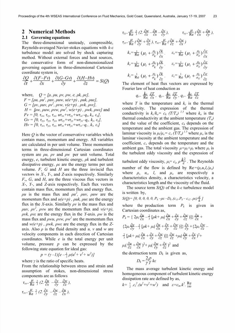
2.1 Governing equations The three-dimensional unsteady, compressible,
Reynolds-averaged Navier-stokes equations with k-ε turbulence model are solved by shock capturing
method. Without external forces and heat sources,the conservative form of non-dimensionalized
governing equation in three-dimensional Cartesian
coordinate system is,
)()()()(
QS z Hv H
yGvG
x Fv F
t Q
=∂−∂
+∂−∂
+∂−∂
+∂∂
where, Q = [ ρ , ρu, ρv, ρw, e, ρk, ρε ],
F = [ ρu, ρu2 , ρuv, ρuw, u(e+p) , ρuk, ρuε ],
G = [ ρv, ρuv, ρv2 , ρvw, v(e+p) , ρvk, ρvε ],
H = [ ρw, ρuw, ρvw, ρw2 , w(e+p) , ρwk, ρwε ] and
Fv = [0, τ xx , τ xy , τ xz , uτ xx+vτ xy+wτ xz –q x , k x , ε x ],Gv = [0, τ xy , τ yy , τ yz , uτ xy+vτ yy+wτ yz –q y , k y , ε y ], Hv = [0, τ xz , τ yz , τ zz , uτ xz +vτ yz +wτ zz –q z , k z , ε z ]
Here Q is the vector of conservative variables which
contain mass, momentum and energy. All variables
are calculated in per unit volume. Three momentum
terms in three-dimensional Cartesian coordinates
system are ρu, ρv and ρw per unit volume. Total
energy, e, turbulent kinetic energy, ρk and turbulent
dissipative energy, ρε are the energy terms per unit
volume. F , G and H are the three inviscid flux
vectors in X -, Y-, and Z -axis respectively. Similarly F v, Gv and H v are the three viscous flux vectors in
X -, Y-, and Z -axis respectively. Each flux vectors
contain mass flux, momentum flux and energy flux.
ρu is the mass flux and ρu2 , ρuv, ρuw are the
momentum flux and u(e+p) , ρuk, ρuε are the energy
flux in the X -axis. Similarly ρv is the mass flux and
ρuv, ρv2 , ρvw are the momentum flux and v(e+p),
ρvk, ρvε are the energy flux in the Y -axis. ρw is the
mass flux and ρwu, ρvw, ρw2are the momentum flux
and w(e+p) , ρwk, ρwε are the energy flux in the Z -axis. Also ρ is the fluid density and u, v and w are
velocity components in each direction of Cartesiancoordinates. While e is the total energy per unit
volume, pressure p can be expressed by the
following state equation for ideal gas:
p = ( γ –1)[e – 21 ρ(u
2+ v
2+ w
2 )]
where γ is the ratio of specific heats.
From the relationship between stress and strain and
assumption of stokes, non-dimensional stress
components are as follows
τ xx= Reµ
32 (2.
xu∂∂ –
yv∂∂ –
z w∂∂ ),
τ yy= Reµ
32 (2. yv∂∂
– z w∂∂ – xu∂∂ ),
τ zz= Reµ
32 (2.
z w∂∂ –
xu∂∂ –
yv
∂∂ ), τ xy= Re
µ (
xv∂∂ +
yu∂∂ ),
τ yz= Reµ
( yw∂∂ +
z v∂∂ ), τ xz= Re
µ (
z u∂∂ +
xw∂∂ )
k x= Re1
x
k
k
t l ∂
∂+ )(σ
µ µ , ε x= Re
1
x
t l
∂
∂+ ε
ε σ
µ µ )(
k y= Re1
y
k
k
t l
∂
∂+ )(σ
µ µ , ε y= Re
1
y
t l
∂
∂+ ε
ε σ
µ µ )(
k z = Re1
z
k
k
t l
∂
∂+ )(σ
µ µ , ε z = Re
1
z
t l
∂
∂+ ε
ε σ
µ µ )(
The element of heat flux vectors are expressed by
Fourier law of heat conduction as
q x= Re
ck xT ∂∂ , q y=
Reck
yT ∂∂ , q z=
Reck
z T ∂∂
where T is the temperature and k c is the thermal
conductivity. The expression of the thermal
conductivity is k c /k o= ck (T/T o )1.5
where k o is the
thermal conductivity at the ambient temperature (T o ) and the value of the coefficient, ck depends on the
temperature and the ambient gas. The expression of
laminar viscosity is µl /µo= cv (T/T o )1.5
where µo is the
laminar viscosity at the ambient temperature and the
coefficient, cv depends on the temperature and the
ambient gas. The total viscosity µ=µl +µt where µt is
the turbulent eddy viscosity and the expression of
turbulent eddy viscosity, µt= c µ. ρ ε
2k . The Reynolds
number of the flow is defined by Re=( ρcucl c /µo ) where ρ
c,u
c , l
cand µ
oare respectively a
characteristics density, a characteristics velocity, a
characteristics length and the viscosity of the fluid.
The source term S(Q) of the k-ε turbulence model
is written by,
S(Q)= [0, 0, 0, 0, 0, P k – ρε –Dk ,(cε1.P k – cε2 . ρε ) k ε ]
where the production term P k is given in
Cartesian coordinates as,
P k = { 2 µt xu∂∂ –
32 [ ρk+ µt( x
u∂∂ +
yv∂∂ +
z w∂∂ )]}
xu∂∂ +
{2 µt yv
∂∂ –
32 [ ρk+ µt( x
u∂∂ +
yv∂∂ +
z w∂∂ )]}
yv
∂∂ +{2 µt z
w∂∂ –
32 [ ρk+ µt( x
u∂∂ +
yv∂∂ +
z w∂∂ )]}
z w∂∂ + µt( y
u∂∂ +
xv∂∂ )2+
µt( z u∂∂ +
xw∂∂ )
2+ µt( y
w∂∂ +
z v∂∂ )
2and
the destruction term Dk is given as,
Dk = T .
2γ
ρ k ε
The mass average turbulent kinetic energy and
homogeneous component of turbulent kinetic energy
dissipation rate are defined by as,
k=21 .ct
2.(u
2+v
2+w
2 ) and ε=cm.k
2.
100Re
Proceedings of the 4th WSEAS International Conference on Fluid Mechanics, Gold Coast, Queensland, Australia, January 17-19, 2007 23
8/3/2019 Mohammad Ali Jinnah- A Numerical Study of Shock Reflection Phenomena in Shock/Turbulence Interaction
http://slidepdf.com/reader/full/mohammad-ali-jinnah-a-numerical-study-of-shock-reflection-phenomena-in-shockturbulence 4/9
The various constants in the k-ε turbulence model
are listed as follows:
c µ=0.09, ct =0.03, cm=0.09, cε1=1.45, cε2=1.92,
σ k =1.00, σ ε=1.30
The following characteristics values are used for
non-dimensionalized in these computations:
Characteristics temperature = 298.00K,Characteristics length = 0.0010 m, Characteristics
pressure = 101000 Pascal, Universal Gas constant = 8.31451, Moleculer weight = 0.029, Ratio of
specific gas constant = 1.4, Characteristics velocity = 292.30 m/s, Characteristics density = 1.1821kg/m3 , Characteristics time = 3.4 µsec, Thermal
conductivity at 0oC = 0.02227 W/m-K, Fluid
viscosity at 0oC = 1.603E-05 Pa.S, Prandtl number
= 0.722, Reynolds number = 21546
The governing equations described above for compressible viscous flow are discretised by the
finite volume method. A second order, upwind
Godounov scheme of Flux vector splitting method is
used to discrete the inviscid flux terms and MUSCL-
Hancock scheme is used for interpolation of
variables. Central differencing scheme is used in
discretizing the viscous flux terms. HLL Reimann
solver is used for shock capturing in the flow. Two
equations for k-ε turbulence model are used to
determine the dissipation of turbulent kinetic energy
and ε the rate of dissipation. The k and ε equations
contain nonlinear production and destruction sourceterms, which can be very large near the solid
boundaries. The upstream of incident shock wave is
set as inflow boundary condition, the properties and
velocities of which are calculated from Rankine-
Hugoniot conditions with incident shock Mach
number. The downstream inflow boundary condition
and wall surface are used as solid boundary
conditions where the gradients normal to the surface
are taken zero. All solid walls are treated as viscous
solid wall boundary. For the two-equation k-ε turbulence model on solid boundaries, µt is set to
zero.
2.2 Grid System and Grid Adaptation
Three dimensional hexahedral cells with adaptive
grids are used for these computations. In this grid
system, the cell-edge data structures are arranged in
such a way that each cell contains six faces which
are sequence in one to six and each face indicates
two neighboring cells that is left cell and right cell
providing all faces of a cell are vectorized by the
position and coordinate in the grid system. The
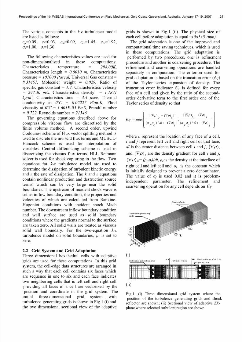
initial three-dimensional grid system with
turbulence-generating grids is shown in Fig.1 (i) and
the two dimensional sectional view of the adaptive
grids is shown in Fig.1 (ii). The physical size of
each cell before adaptation is equal to 5x5x5 (mm). The grid adaptation is one of the improved and
computational time saving techniques, which is used
in these computations. The grid adaptation is
performed by two procedures, one is refinement
procedure and another is coarsening procedure. The
refinement and coarsening operations are handled
separately in computation. The criterion used for
grid adaptation is based on the truncation error (Є T )
of the Taylor series expansion of density. The
truncation error indicator Є T is defined for every
face of a cell and given by the ratio of the second-
order derivative term to the first order one of the
Taylor series of density so that
Є T = max
∇+
∇−∇
∇+
∇−∇
|)(|/)(
|)()(|
,|)(|/)(
|)()(|
jdl
f
jlc
idl
f
ilc
ccρ ρ α
ρ ρ
ρ ρ α
ρ ρ
where c represent the location of any face of a cell,
i and j represent left cell and right cell of that face,
dl is the center distance between cell i and j, )( ρ ∇ i
and )( ρ ∇ j are the density gradient for cell i and j,
)( ρ ∇ lc= ( ρi- ρ j )/dl , ρc is the density at the interface of
right cell and left cell and α f is the constant which
is initially designed to prevent a zero denominator.
The value of α f is used 0.02 and it is problem-
independent parameter. The refinement andcoarsening operation for any cell depends on Є T
Turbulence-generating
grids
Shock reflector
(i)
Turbulence-generating gridsShock reflector of 49.0 %
opening areaTurbulent region
AA BB
(ii)
Fig.1: (i) Three dimensional grid system where the
position of the turbulence generating grids and shock reflector are shown; (ii) Sectional view of adaptive ZX -
plane where selected turbulent region are shown
Proceedings of the 4th WSEAS International Conference on Fluid Mechanics, Gold Coast, Queensland, Australia, January 17-19, 2007 24

8/3/2019 Mohammad Ali Jinnah- A Numerical Study of Shock Reflection Phenomena in Shock/Turbulence Interaction
http://slidepdf.com/reader/full/mohammad-ali-jinnah-a-numerical-study-of-shock-reflection-phenomena-in-shockturbulence 5/9
value and the value of Є T is determined for each face
of a cell. The criterion for adaptation for any cell isRefinement = maximum Є T of six faces of a cell >εr
Coarsening = maximum Є T of six faces of a cell <εc where εr and εc are the threshold values for
refinement and coarsening. In these computations,
the value of εr is used 0.44 and the value of εc is used0.40 and the level of refinement is 3.
In the refinement procedure, the cells are selected
for refinement in which every cell is divided into
eight new sub cells and these new sub cells are
arranged in a particular sequence so that these sub
cells are used suitably in the data-structure. In the
coarsening procedure, the eight sub cells, which are
generated from the primary cell, are restored into the
primary cell. The above three-dimensional
adaptation strategy is an upgraded work of two-
dimensional adaptation developed by Sun andTakayama [8].
3 Results and DiscussionIn this paper, the investigation on shock reflection
phenomena from different shock reflectors is
focused mainly to enhance the reflected shock
utilities in the shock/turbulence interaction. The
incident shock utilities in the shock/turbulence
interaction are the difficult task due to generation of
the homogeneous turbulence field and the
generation of the incident shock simultaneously. Inthat case, the reflected shock utilities in interaction
with grid-generated shock-induced turbulence are
the suitable techniques. Many researchers were used
shock reflection technique from the plane end wall
and they used shock-induced turbulent flow in the
wake of the turbulence grid for the interaction. In
the present computations, different shock reflectors
of 49.0 % and 26.5 % opening area are used to get
the different strengths of reflected shock wave and
these results are compared with the results for the
reflection from the plane end wall. In the present
computations, the time-dependent Reynolds-
averaged Navier-Stokes equations with k-ε turbulence model are solved by the grid adaptation
technique. All the relevant parameters are resolved
with k-ε turbulence model for shock Mach number,
M s = 2.00. Navier-Stokes simulation (NS) is also
performed to observe the present shock reflection
phenomena with the same incident shock wave. The
Navier-Stokes simulation (NS) results are used to
compare with the present simulation results and it is
observed that there have good agreements between
the present simulation results and the NS results.After the partial reflection from different shock
reflectors, different strengths of the reflected shock
wave interact with the same strength of turbulence
field. Shock reflector is the device and it has both
the reflection and transmitting capabilities of the
shock wave. Shock reflectors are classified by the
open area ratio. Two types of shock reflectors are
used which are shown in Fig.2 (i) and (ii). Shock
reflector of 49.0 % opening area has more
transmitting capabilities of the shock wave as
compare to the shock reflector of 26.5 % opening
area. The strength of the reflected shock wave after
partial reflection from the reflector of 49.0 %
opening area is comparatively weaker than the
strength of the reflected shock wave after partial
reflection from the reflector of 26.5 % opening area.
On the other hand, the incident shock Mach number
and the configuration of turbulence grid plate are
same for all computations. So the strength of the
shock induced turbulent flow in the wake of theturbulence grid is same for all types of
computations.
To generate a compressible flow of homogeneous,
isotropic turbulence, turbulence-generating grids are
placed in the shock tube parallel to YZ- plane, which
is shown in Fig.1. The total opening area of
turbulence-generating grids is 51.0 % and the
configuration of the turbulence-generating grids is
shown in Fig.2 (iii). Turbulence-generating grids are
uniform in size and spacing; so the shock wave and
the gas flow following the shock wave after passing
through turbulence-generating grids generate acompressible flow of homogeneous, isotropic
turbulence. The region between the lateral plane AA
and BB in Fig.1 (ii), is treated as the selected
turbulent region. The centerline, along the
longitudinal direction of the turbulent region is
treated as the centerline of the turbulent region. 15
points of equal spacing are taken on the centerline of
the turbulent region and different parameters
(velocity, pressure and temperature etc.) are
computed on these 15 points. The lateral planes
intersect these points and parallel to the YZ -plane are
(i) (ii) (iii)
Fig.2: (i) The configuration of shock reflector of 49.0 %
opening area (ii) The configuration of shock reflector of 26.5 % opening area (iii) The configuration of turbulence-
generating grids
Proceedings of the 4th WSEAS International Conference on Fluid Mechanics, Gold Coast, Queensland, Australia, January 17-19, 2007 25
8/3/2019 Mohammad Ali Jinnah- A Numerical Study of Shock Reflection Phenomena in Shock/Turbulence Interaction
http://slidepdf.com/reader/full/mohammad-ali-jinnah-a-numerical-study-of-shock-reflection-phenomena-in-shockturbulence 6/9
treated as the grid-data planes and the grids inside
the turbulent region cut by the grid-data planes are
the grids on the grid-data plane. The value of the
turbulent parameter on the center line of the
turbulent region is the average value of all the grid
values of that parameter on the grid-data plane and
in the present computations, the grids adjacent to the
boundary are not taken into account due to viscous
effect. The pressure, velocity and temperature etc,
are determined across the reflected shock wave
when the position of the reflected shock wave is in
the turbulent region and the characteristics profiles
of these parameters across the reflected shock wave
are plotted to observe the reflection phenomena. The
longitudinal distance ( X/m) of any point on the
centerline of the turbulent region are determined
from the turbulence-generating girds where m = 5.0
mm, the maximum dimensional length of a grid inthe grid system. The distance, X = 0.0 mm at the
position of turbulence-generating grids. The value,
X/m = 6.9 is the starting point of the centerline and
the value, X/m = 18.2 is the ending point of the
centerline of the turbulent region.
After the shock wave is diffracted through the
turbulence grids, the fluid flow causes the formation
of unsteady, compressible vortices and the vortices
separate from the grids, then merges, dissipates and
forms a compressible turbulent field at some
distance downstream of the grids. It is observed that
near the turbulence grids, the unsteady vorticityfluctuations in the lateral direction are high which
cause more flow fluctuations in the lateral direction.
The vortex fluctuations as well as vortex interaction
change to fully developed turbulence field in the
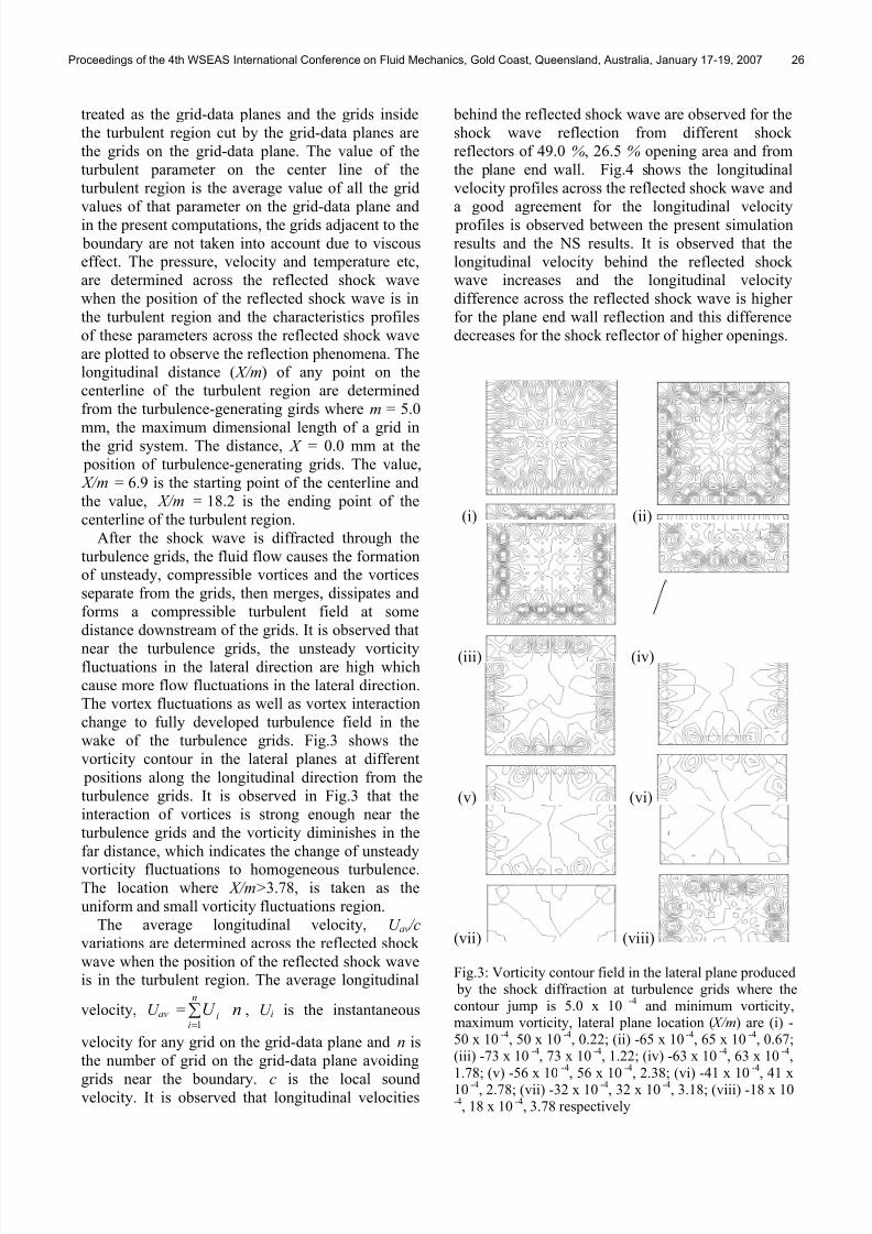
wake of the turbulence grids. Fig.3 shows the
vorticity contour in the lateral planes at different
positions along the longitudinal direction from the
turbulence grids. It is observed in Fig.3 that the
interaction of vortices is strong enough near the
turbulence grids and the vorticity diminishes in the
far distance, which indicates the change of unsteady
vorticity fluctuations to homogeneous turbulence.The location where X/m>3.78, is taken as the
uniform and small vorticity fluctuations region.
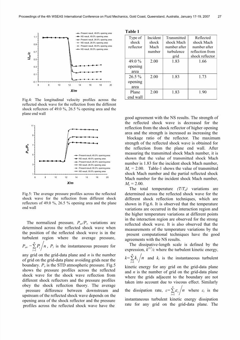
The average longitudinal velocity, U av /cvariations are determined across the reflected shock
wave when the position of the reflected shock wave
is in the turbulent region. The average longitudinal
velocity, U av = nU n
ii∑
=1
, U i is the instantaneous
velocity for any grid on the grid-data plane and n is
the number of grid on the grid-data plane avoiding
grids near the boundary. c is the local soundvelocity. It is observed that longitudinal velocities
behind the reflected shock wave are observed for the
shock wave reflection from different shock
reflectors of 49.0 %, 26.5 % opening area and from
the plane end wall. Fig.4 shows the longitudinal
velocity profiles across the reflected shock wave and
a good agreement for the longitudinal velocity
profiles is observed between the present simulation
results and the NS results. It is observed that the
longitudinal velocity behind the reflected shock
wave increases and the longitudinal velocity
difference across the reflected shock wave is higher
for the plane end wall reflection and this difference
decreases for the shock reflector of higher openings.
(i) (ii)
(iii) (iv)
(v) (vi)
(vii) (viii)
Fig.3: Vorticity contour field in the lateral plane produced by the shock diffraction at turbulence grids where thecontour jump is 5.0 x 10
-4and minimum vorticity,
maximum vorticity, lateral plane location ( X/m) are (i) -50 x 10 -4, 50 x 10 -4, 0.22; (ii) -65 x 10 -4, 65 x 10 -4, 0.67;(iii) -73 x 10 -4, 73 x 10 -4, 1.22; (iv) -63 x 10 -4, 63 x 10 -4,
1.78; (v) -56 x 10-4
, 56 x 10-4
, 2.38; (vi) -41 x 10-4
, 41 x10 -4, 2.78; (vii) -32 x 10 -4, 32 x 10 -4, 3.18; (viii) -18 x 10
-4, 18 x 10
-4, 3.78 respectively
Proceedings of the 4th WSEAS International Conference on Fluid Mechanics, Gold Coast, Queensland, Australia, January 17-19, 2007 26
8/3/2019 Mohammad Ali Jinnah- A Numerical Study of Shock Reflection Phenomena in Shock/Turbulence Interaction
http://slidepdf.com/reader/full/mohammad-ali-jinnah-a-numerical-study-of-shock-reflection-phenomena-in-shockturbulence 7/9
-0.1
0.1
0.3
0.5
0.7
0.9
1.1
6 8 10 12 14 16 18 20
X/m
U
a v
/ c
Present result, 49.0% opening area
NS result, 49.0% opening area
Present result, 26.5% opening area
NS result, 26.5% opening area
Present result, 00.0% opening area
NS result, 00.0% opening area
Fig.4: The longitudinal velocity profiles across thereflected shock wave for the reflection from the differentshock reflectors of 49.0 %, 26.5 % opening area and the plane end wall
1
3
5
7
9
11
6 8 10 12 14 16 18 20
X/m
P a v / P o
Present result, 49.0% opening area
NS result, 49.0% opening area
Present result, 26.5% opening area
NS result, 26.5% opening area
Present result, 00.0% opening area
NS result, 00.0% opening area
Fig.5: The average pressure profiles across the reflectedshock wave for the reflection from different shock
reflectors of 49.0 %, 26.5 % opening area and the planeend wall
The normalized pressure, P av /P o variations are
determined across the reflected shock wave when
the position of the reflected shock wave is in the
turbulent region where the average pressure,
P av = n P n
ii∑
=1
, P i is the instantaneous pressure for
any grid on the grid-data plane and n is the number
of grid on the grid-data plane avoiding grids near the
boundary. P o is the STD atmospheric pressure. Fig.5
shows the pressure profiles across the reflected
shock wave for the shock wave reflection from
different shock reflectors and the pressure profiles
obey the shock reflection theory. The average
pressure difference between downstream and
upstream of the reflected shock wave depends on the
opening area of the shock reflector and the pressure
profiles across the reflected shock wave have the
Table 1
Type of shock
reflector
Incidentshock
Machnumber
Transmittedshock Mach
number after turbulence
grid
Reflectedshock Machnumber after
reflection fromshock reflector
49.0 %
opening
area
2.00 1.83 1.66
26.5 %
opening
area
2.00 1.83 1.73
Plane
end wall
2.00 1.83 1.90
good agreement with the NS results. The strength of the reflected shock wave is decreased for the
reflection from the shock reflector of higher opening
area and the strength is increased as increasing the
blockage ratio of the reflector. The maximum
strength of the reflected shock wave is obtained for
the reflection from the plane end wall. After
measuring the transmitted shock Mach number, it is
shown that the value of transmitted shock Mach
number is 1.83 for the incident shock Mach number,
M s = 2.00. Table-1 shows the value of transmitted
shock Mach number and the partial reflected shock
Mach number for the incident shock Mach number,M s = 2.00.
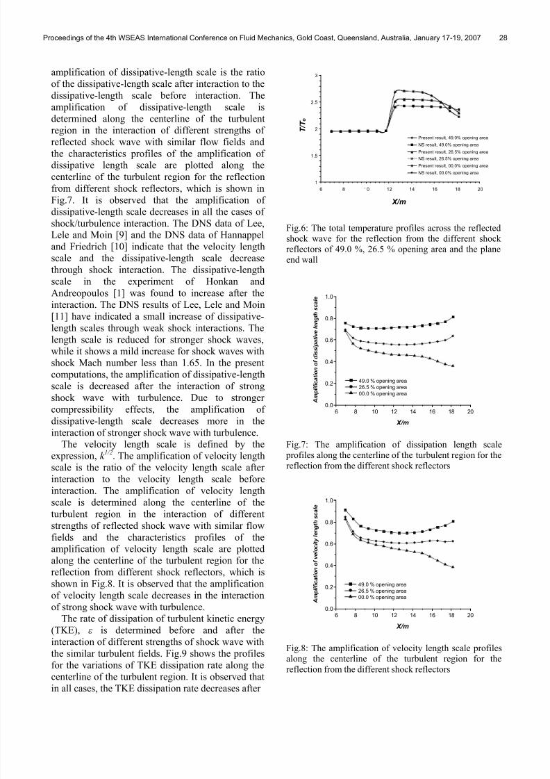
The total temperature (T/T o ) variations are
determined across the reflected shock wave for the
different shock reflection techniques, which are
shown in Fig.6. It is observed that the temperature
variations are occurred in the interaction region and
the higher temperature variations at different points
in the interaction region are observed for the strong
reflected shock wave. It is also observed that the
measurements of the temperature variations by the
present computational techniques have the good
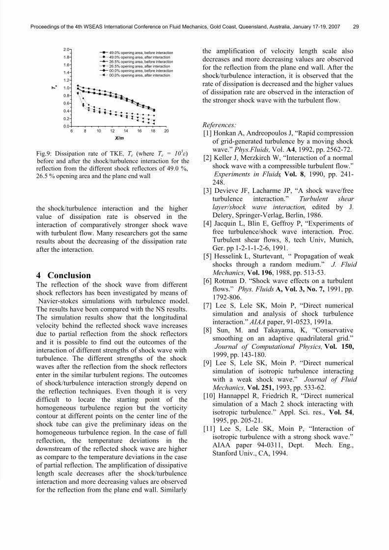
agreements with the NS results.The dissipative-length scale is defined by the
expression, k 3/2
/ ε where the turbulent kinetic energy,
k= nk n
ii∑
=1
and k i is the instantaneous turbulent
kinetic energy for any grid on the grid-data plane
and n is the number of grid on the grid-data plane
where the grids adjacent to the boundary are not
taken into account due to viscous effect. Similarly
the dissipation rate, ε= nn
ii∑
=1
ε where εi is the
instantaneous turbulent kinetic energy dissipationrate for any grid on the grid-data plane. The
Proceedings of the 4th WSEAS International Conference on Fluid Mechanics, Gold Coast, Queensland, Australia, January 17-19, 2007 27
8/3/2019 Mohammad Ali Jinnah- A Numerical Study of Shock Reflection Phenomena in Shock/Turbulence Interaction
http://slidepdf.com/reader/full/mohammad-ali-jinnah-a-numerical-study-of-shock-reflection-phenomena-in-shockturbulence 8/9
8/3/2019 Mohammad Ali Jinnah- A Numerical Study of Shock Reflection Phenomena in Shock/Turbulence Interaction
http://slidepdf.com/reader/full/mohammad-ali-jinnah-a-numerical-study-of-shock-reflection-phenomena-in-shockturbulence 9/9
6 8 10 12 14 16 18 200.0
0.2
0.4
0.6
0.8
1.0
1.2
1.4
1.6
1.8
2.0
T e
X/m
49.0% opening area, before interaction
49.0% opening area, after interaction
26.5% opening area, before interaction
26.5% opening area, after interaction
00.0% opening area, before interaction
00.0% opening area, after interaction
Fig.9: Dissipation rate of TKE, T e (where T e = 105ε)
before and after the shock/turbulence interaction for thereflection from the different shock reflectors of 49.0 %,
26.5 % opening area and the plane end wall
the shock/turbulence interaction and the higher
value of dissipation rate is observed in the
interaction of comparatively stronger shock wave
with turbulent flow. Many researchers got the same
results about the decreasing of the dissipation rate
after the interaction.
4 ConclusionThe reflection of the shock wave from different
shock reflectors has been investigated by means of
Navier-stokes simulations with turbulence model.
The results have been compared with the NS results.
The simulation results show that the longitudinal
velocity behind the reflected shock wave increases
due to partial reflection from the shock reflectors
and it is possible to find out the outcomes of the
interaction of different strengths of shock wave with
turbulence. The different strengths of the shock
waves after the reflection from the shock reflectors
enter in the similar turbulent regions. The outcomes
of shock/turbulence interaction strongly depend onthe reflection techniques. Even though it is very
difficult to locate the starting point of the
homogeneous turbulence region but the vorticity
contour at different points on the center line of the
shock tube can give the preliminary ideas on the
homogeneous turbulence region. In the case of full
reflection, the temperature deviations in the
downstream of the reflected shock wave are higher
as compare to the temperature deviations in the case
of partial reflection. The amplification of dissipative
length scale decreases after the shock/turbulence
interaction and more decreasing values are observedfor the reflection from the plane end wall. Similarly
the amplification of velocity length scale also
decreases and more decreasing values are observed
for the reflection from the plane end wall. After the
shock/turbulence interaction, it is observed that the
rate of dissipation is decreased and the higher values
of dissipation rate are observed in the interaction of
the stronger shock wave with the turbulent flow.
References:[1] Honkan A, Andreopoulos J, “Rapid compression
of grid-generated turbulence by a moving shock
wave.” Phys.Fluids, Vol. A4, 1992, pp. 2562-72.
[2] Keller J, Merzkirch W, “Interaction of a normal
shock wave with a compressible turbulent flow.”
Experiments in Fluids, Vol. 8, 1990, pp. 241-
248.
[3] Devieve JF, Lacharme JP, “A shock wave/freeturbulence interaction.” Turbulent shear layer/shock wave interaction, edited by J.
Delery, Springer-Verlag, Berlin, 1986.
[4] Jacquin L, Blin E, Geffroy P, “Experiments of
free turbulence/shock wave interaction. Proc.
Turbulent shear flows, 8, tech Univ, Munich,
Ger. pp 1-2-1-1-2-6, 1991.
[5] Hesselink L, Sturtevant, “ Propagation of weak
shocks through a random medium.” J. Fluid Mechanics, Vol. 196, 1988, pp. 513-53.
[6] Rotman D. “Shock wave effects on a turbulent
flows.” Phys. Fluids A, Vol. 3, No. 7, 1991, pp.1792-806.
[7] Lee S, Lele SK, Moin P, “Direct numerical
simulation and analysis of shock turbulence
interaction.” AIAA paper, 91-0523, 1991a.
[8] Sun, M. and Takayama, K, “Conservative
smoothing on an adaptive quadrilateral grid.”
Journal of Computational Physics, Vol. 150,
1999, pp. 143-180.
[9] Lee S, Lele SK, Moin P. “Direct numerical
simulation of isotropic turbulence interacting
with a weak shock wave.” Journal of Fluid
Mechanics, Vol. 251, 1993, pp. 533-62.[10] Hannappel R, Friedrich R, “Direct numerical
simulation of a Mach 2 shock interacting with
isotropic turbulence.” Appl. Sci. res., Vol. 54,
1995, pp. 205-21.
[11] Lee S, Lele SK, Moin P, “Interaction of
isotropic turbulence with a strong shock wave.”
AIAA paper 94-0311, Dept. Mech. Eng.,
Stanford Univ., CA, 1994.
Proceedings of the 4th WSEAS International Conference on Fluid Mechanics, Gold Coast, Queensland, Australia, January 17-19, 2007 29