1 | P a g e

Module G:

Turbulent Compressible / Incompressible Flow Over an Isolated Airfoil

Summary…………………………………………….

Problem Statement…………………………………

Problem Setup………………………………..……

Turbulent Compressible Case………………………

Turbulent Incompressible Case……………………

Solution………………………………...……………

Postprocessing and Validation………………………

Summary

This learning module introduces the user to analyzing turbulent external flow past an airfoil.

Two cases are considered—compressible and incompressible flow for various angles of attack.

An already created mesh is used provided in Tutorial 3—External Compressible Flow on the

Senior Design Project Website. The main difference between the two tutorials is that this module

provides the means of validating the obtained results in order for the user to verify the data

obtained is meaningful. This module as mentioned also demonstrates how to successfully change

the parameters in ANSYS Fluent in order to obtain data for incompressible flow. Finally this

module examines the difference between different turbulence methods for a particular angle of

attack.

By having completed this learning module the user with confidence can set up properly turbulent

compressible and incompressible flows across an airfoil in FLUENT. This will be crucial in the

next module—Turbulent Incompressible Flow across a Periodic Airfoil. In the next module it

will be assumed the user knows how to setup the case in FLUENT and special attention will be

paid to the geometry and meshing of the problem as that is where the difficulty lies. This

learning module has exposed the user to the theory of lift and its use in the validation of the

experimental data. Further flexibility of FLUENT is exposed since the mesh has been created in

GAMBIT. By demonstrating in-depth the separation of zones in FLUENT, the user has learned

2 | P a g e

another important tool in proper problem setup since sometimes it becomes necessary to import

mesh files which cannot be viewed in Workbench to have their named zones manipulated.

Finally further validation methods are illustrated to ensure the obtained data makes sense.

Problem Statement:

Consider a symmetrical NACA0012 airfoil of chord length c=1 m. For the compressible

case, the free stream Mach number is 0.8 and for the incompressible case is 2.

The lift coeffiicent and the drag coefficient will be obtained from Fluent for

various angles of attack, α.

Fig.G.1 Airfoil geometry definition

Eq. [1] is used to compute the Reynolds number for both cases—compressible and

incompressible. A Mach number of 0.8 has a velocity approximately 272.0 m/s and a

Mach number of 0.2 is approximately 68 m/s. As it can be seen in both cases, the

Reynolds number is well into the turbulent region since the values are greater than

500,000.

Chord Reynolds Number (1)

where: c is the chord length in meters, V is free-stream velocity in m/s and 70,000 is the

kinematic viscosity for air

Compressible Case

R , Incompressible Case

Problem Setup:

Open ANSYS Fluent. In the Fluent Launcher specify the dimension as 2D. Under

Options select Double Precision for better accuracy.

Under General Options specify the working directory for easier access. This will save

time when saving, reading cases, etc. Press OK.

c=1m 𝑀∞

α

3 | P a g e

Fig.G.2

An already created C-grid mesh (made in Gambit-old Fluent mesh generator) is to be

used for this module. The mesh can be downloaded from:

http://www.engr.uconn.edu/~barbertj/CFD%20Training/Fluent%2012/Tut%2003-

modeling%20external%20compressible%20flow/

Download airfoil.msh file to the working directory. In Fluent, Select File-Read-Mesh.

Double click airfoil.msh.

Fig.G.3 Gambit generated mesh

4 | P a g e

External Turbulent Compressible Flow Across an Airfoil:

Problem Setup-Models:

Keep the defaults in Problem Setup-General.

Fig.G.4

In Problem Setup-Models, double click on the default Viscous-Laminar and specify the

Spalart-Allmaras turbulence method. Under Spalart-Allmaras Production specify

Strain/Vorticity-Based. This turbulence, one equation, model is relatively simple and is

well suited for aerospace applications (wall-bounded flows) and provides good results for

boundary layers subjected to adverse pressure gradients. Press OK.

Fig.G.5

5 | P a g e

Problem Setup-Materials:

In Problem Setup-Materials, double click on Air. Since first we are to analyze turbulent

compressible flow (properties are no longer constant), change the density to ideal gas.

For viscosity specify Sutherland and keep the defaults—Three Coefficient Method. The

Sutherland method is well suited for high-speed compressible flows.

For simplicity purposes let the specific heat and thermal conductivity be constant.

Fig.G.6

Fig.G.7

Finally click on Change/Create. The specified parameters have overwritten the Air

material.

It is important to note that had the specified parameters been saved as a different material

name (without overwriting the pre-existing material) for example compressible_material,

an extra step is required to be taken in order for accurate results to be obtained.

6 | P a g e

In Problem Setup-Cell Zone Conditions, double click on the fluid-16 zone. Next to

Material Name specify the material name, in this case—compressible_material. Press

OK.

Fig.G.8

Note that the Energy Equation has been turned on automatically since density is not

constant anymore. Verify by going back to Problem Setup-Models. Energy-On should

be visible.

7 | P a g e

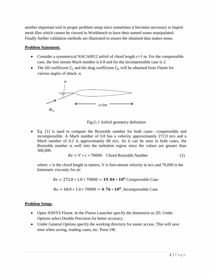
Problem Setup-Boundary Conditions:

Next the Boundary Conditions are specified.

Fig.G.9 Boundary condition definitions – compressible airfoil case

interior

Pressure-far-field

Pressure-far-field

Pressure-far-field

Wall-top

Wall-bottom

8 | P a g e

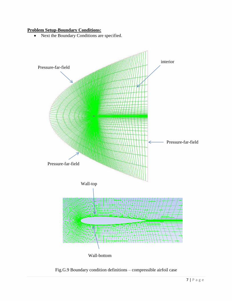
In Problem Setup-Boundary Conditions, verify that the wall-top, wall-bottom zones

are of type wall; that zone interior-1 is of type interior; that zone pressure-far-field-1 is of

type pressure-far-field.

Click on Operating Conditions and verify the operating pressure is set at 101, 325 Pa.

Double click on the pressure-far-field-1 zone.

For the turbulent case which is considered first set the Mach number at 0.8; the gauge

pressure should be left at 0.

The x and y components of flow direction depend on the angle of attack, for example if

angle of attack of 6 degrees is considered, the x-component of flow direction should be

set to the numerical value of while the y-component of flow direction should be

set to the numerical value of and so on for other values of the angle of attack.

For Turbulence-Specification Method, select Turbulent Viscosity Ratio and keep the

default of 10.

Fig.G.10

In the Thermal Tab verify the Temperature is set at 300K. Press OK.

9 | P a g e

Problem Setup-Reference Values:

In Problem Setup-Reference Values, set the reference values to be computed from the

pressure-far-field-1 zone.

Fig.G.11

Solution:

In Solution –Solution Methods, under Scheme select Coupled.

Under Spatial Discretization keep the defaults for Gradient-Least Square Cell Based, and

for pressure-standard.

Specify Second Order Upwind for density, momentum, modified turbulent viscosity and

energy. Doing so will increase the accuracy of the solution however it will take longer to

obtain convergence.

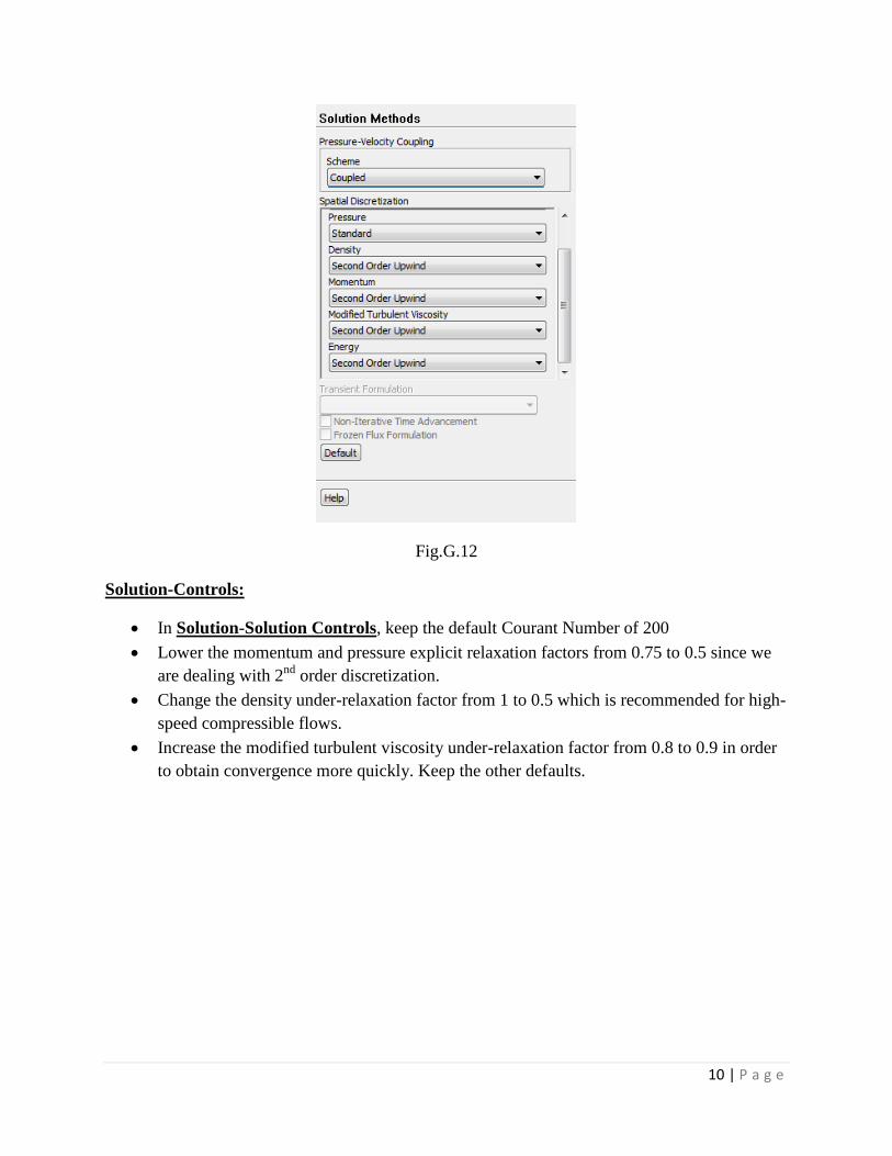
10 | P a g e

Fig.G.12

Solution-Controls:

In Solution-Solution Controls, keep the default Courant Number of 200

Lower the momentum and pressure explicit relaxation factors from 0.75 to 0.5 since we

are dealing with 2nd

order discretization.

Change the density under-relaxation factor from 1 to 0.5 which is recommended for high-

speed compressible flows.

Increase the modified turbulent viscosity under-relaxation factor from 0.8 to 0.9 in order

to obtain convergence more quickly. Keep the other defaults.

11 | P a g e

Fig.G.13

Solution-Monitors:

In Solution-Monitors double click on Residuals. Make sure Print to Console and Plot are

checked.

In Equations specify the absolute criteria as 1e-06 for all 5 equations. Press OK.

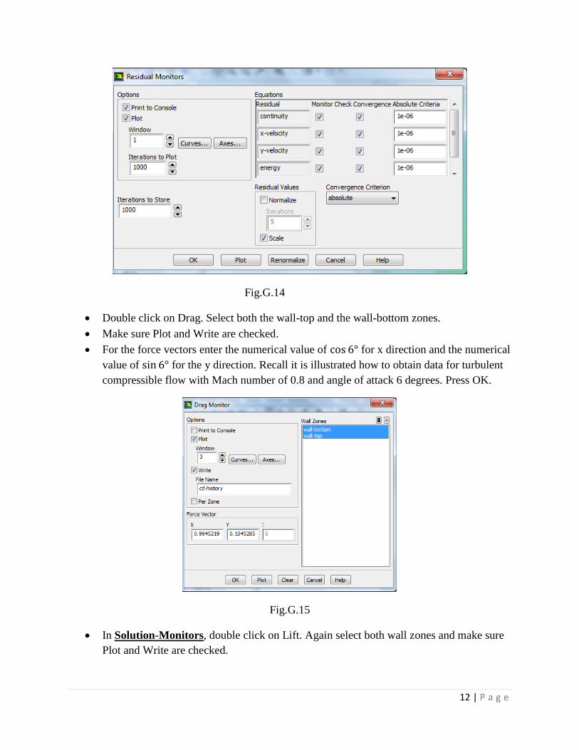
12 | P a g e

Fig.G.14

Double click on Drag. Select both the wall-top and the wall-bottom zones.

Make sure Plot and Write are checked.

For the force vectors enter the numerical value of for x direction and the numerical

value of for the y direction. Recall it is illustrated how to obtain data for turbulent

compressible flow with Mach number of 0.8 and angle of attack 6 degrees. Press OK.

Fig.G.15

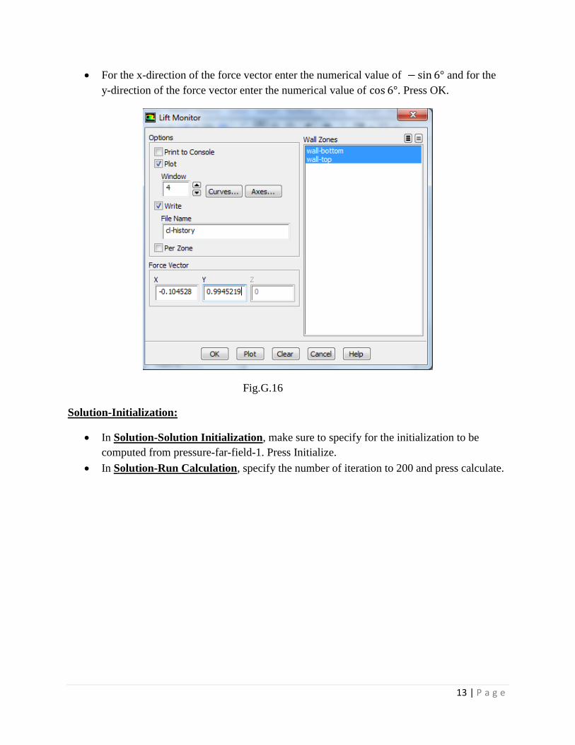
In Solution-Monitors, double click on Lift. Again select both wall zones and make sure

Plot and Write are checked.

13 | P a g e

For the x-direction of the force vector enter the numerical value of and for the

y-direction of the force vector enter the numerical value of . Press OK.

Fig.G.16

Solution-Initialization:

In Solution-Solution Initialization, make sure to specify for the initialization to be

computed from pressure-far-field-1. Press Initialize.

In Solution-Run Calculation, specify the number of iteration to 200 and press calculate.

14 | P a g e

Fig.G.17 Solution residual iteration history

Fig.G.18 Compressible lift coefficient iteration history

15 | P a g e

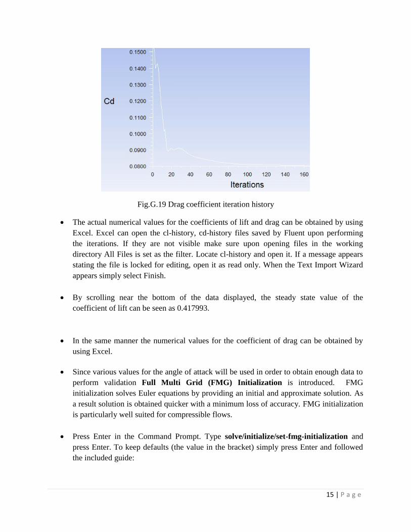
Fig.G.19 Drag coefficient iteration history

The actual numerical values for the coefficients of lift and drag can be obtained by using

Excel. Excel can open the cl-history, cd-history files saved by Fluent upon performing

the iterations. If they are not visible make sure upon opening files in the working

directory All Files is set as the filter. Locate cl-history and open it. If a message appears

stating the file is locked for editing, open it as read only. When the Text Import Wizard

appears simply select Finish.

By scrolling near the bottom of the data displayed, the steady state value of the

coefficient of lift can be seen as 0.417993.

In the same manner the numerical values for the coefficient of drag can be obtained by

using Excel.

Since various values for the angle of attack will be used in order to obtain enough data to

perform validation Full Multi Grid (FMG) Initialization is introduced. FMG

initialization solves Euler equations by providing an initial and approximate solution. As

a result solution is obtained quicker with a minimum loss of accuracy. FMG initialization

is particularly well suited for compressible flows.

Press Enter in the Command Prompt. Type solve/initialize/set-fmg-initialization and

press Enter. To keep defaults (the value in the bracket) simply press Enter and followed

the included guide:

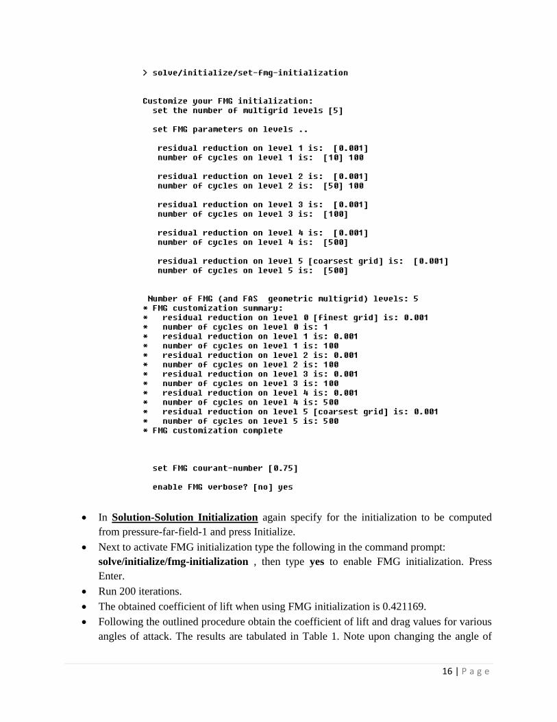
16 | P a g e

In Solution-Solution Initialization again specify for the initialization to be computed

from pressure-far-field-1 and press Initialize.

Next to activate FMG initialization type the following in the command prompt:

solve/initialize/fmg-initialization , then type yes to enable FMG initialization. Press

Enter.

Run 200 iterations.

The obtained coefficient of lift when using FMG initialization is 0.421169.

Following the outlined procedure obtain the coefficient of lift and drag values for various

angles of attack. The results are tabulated in Table 1. Note upon changing the angle of

17 | P a g e

attack the new numerical value must be entered in the pressure-far-field-1 boundary

condition as well as in the drag and lift force monitors. Also remember to both initialize

from the pressure-far-field-1 and to enable FMG initialization for each new angle of

attack under consideration. Depending on the number of significant figures used when

entering various parameters the obtained results might differ slightly from the provided

ones.

External Turbulent Incompressible Flow Across an Airfoil:

Two methods are possible for obtaining data for external turbulent incompressible flow

across the provided airfoil and boundary conditions.

o The first case is to use the already defined pressure-far-field boundary zone which

means the energy equation will have to stay turned on and the material properties

for the air material will remain the same. Specifically the density will remain as

ideal gas and the viscosity will continue to follow the Sutherland model. The only

change will be to lower the velocity in the pressure-far-field boundary

condition—now for the incompressible case it is to be specified as M=0.2. This

method of obtaining results for the incompressible case is very easy to implement

and due to its triviality will be left to the user to explore.

o The second method of obtaining data for the incompressible case is to actually

separate the pressure-far-field boundary zone into two zones which are to be

defined as pressure outlet and velocity inlet. Doing so will enable us to turn off

the energy equation and the material properties for air can now be specified as

constant following the definition of incompressible flow. The issue stems from

the fact that for a pressure-far-field boundary conditions the density must be

specified as ideal gas meaning the pressure-far-field is designed for compressible

analysis. The outlined method will be discussed in depth since new methods of

manipulating the boundary conditions are introduced to the user. This method also

will yield more accurate results than the first method of modeling incompressible

flow discussed in the previous paragraph.

First save the turbulent compressible case and data—File—Write—Case and Data.

In order to manipulate the pressure-far-field boundary and separate it into two distinct zones,

first make sure the geometry is visible (Problem Setup—General—Display and select the

pressure-far-field-1 surface). Recall the limits of the domain (Problem Setup—General—

Scale)—Fig.G.20.

18 | P a g e

Fig.G.20

Then go to the Adapt—Region. Enter the coordinates as outlined in Fig.G.21 and press

Mark.

Fig.G.21

Finally proceed to Mesh—Separate and choose Faces. Select Mark under Options and

specify the created register and zone as outlined in Fig.G.22. Then press Separate.

Fig.G.22

19 | P a g e

The original pressure far field zone is now separated into two zones to be specified as

velocity inlet and pressure outlet as outlined in Fig.G.23:

Fig.G.23 Boundary condition definition for incompressible case

Interior

Velocity-inlet

Velocity-inlet

Pressure-outlet

Wall-top

Wall-bottom

20 | P a g e

In Problem Setup—Materials, double click on air and specify density and viscosity as

constant.

Fig.G.24

In Problem Setup—Boundary Conditions, double click on pressure-far-field-1. That zone

should now be specified as velocity inlet. Specify the free-stream velocity as 68 m/s which is

about 0.2 Mach.

Fig.G.25

21 | P a g e

The pressure-far-field-1:002 zone is specified as pressure outlet.

Fig.G.26

Verify the energy equation in Problem Setup—Models is turned off.

Apart from the described changes specifically energy equation turned off, density and

viscosity being constant, the newly specified velocity-inlet and pressure-outlet boundaries,

everything else remains absolutely the same. Just make sure the reference values are

computed from the inlet—pressure-far-field-1.The same approach is continued to obtain

convergence as outlined in the compressible case.

Post-Processing and Validation:

The first validation to be performed is for the coefficient of lift as a function of the angle

of attack. It will be validated against the equation for the coefficient of lift as provided by

the circulation theory of lift:

(2)

where α is in radians, i.e. ⁄ 0.01745 rad. Eq. [1] is a theoretical model

developed for an ideal flow [incompressible, inviscid].

22 | P a g e

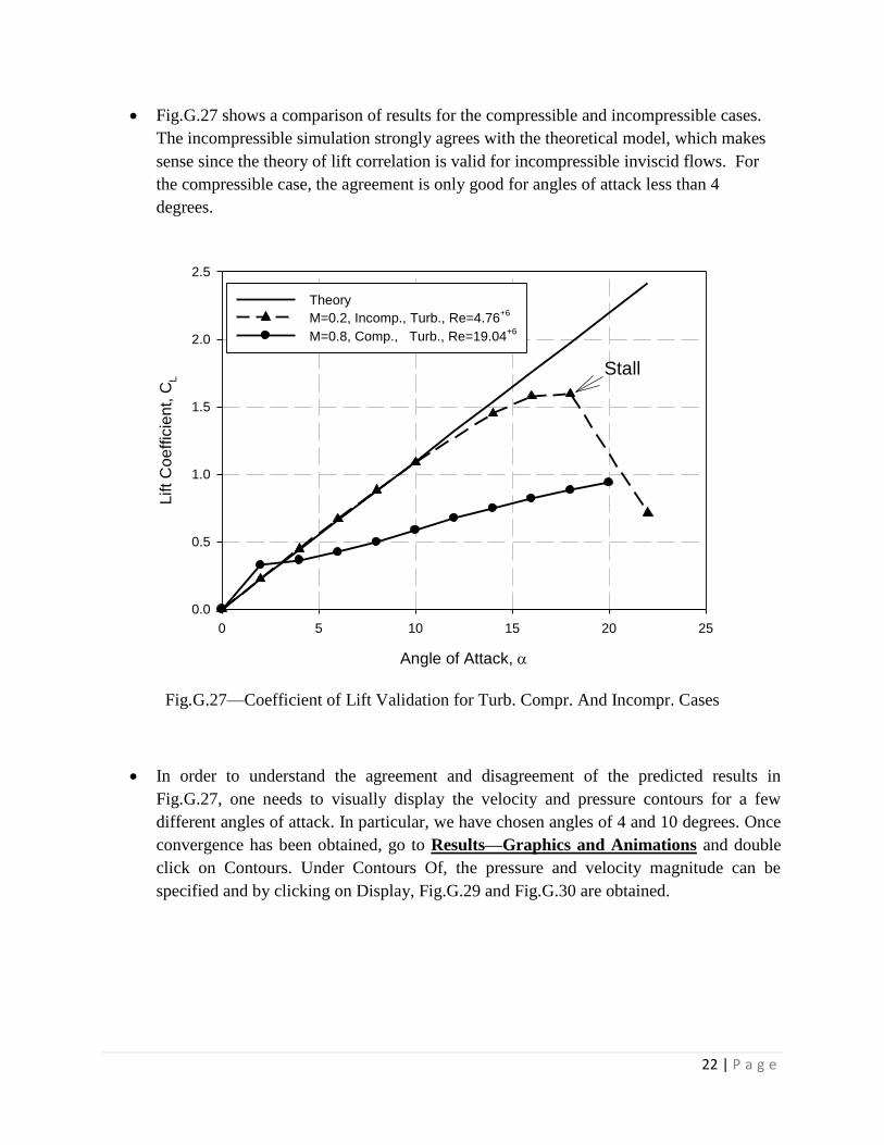
Fig.G.27 shows a comparison of results for the compressible and incompressible cases.

The incompressible simulation strongly agrees with the theoretical model, which makes

sense since the theory of lift correlation is valid for incompressible inviscid flows. For

the compressible case, the agreement is only good for angles of attack less than 4

degrees.

Angle of Attack,

0 5 10 15 20 25

Lift C

oe

ffic

ien

t, C

L

0.0

0.5

1.0

1.5

2.0

2.5

Theory

M=0.2, Incomp., Turb., Re=4.76+6

M=0.8, Comp., Turb., Re=19.04+6

Stall

Fig.G.27—Coefficient of Lift Validation for Turb. Compr. And Incompr. Cases

In order to understand the agreement and disagreement of the predicted results in

Fig.G.27, one needs to visually display the velocity and pressure contours for a few

different angles of attack. In particular, we have chosen angles of 4 and 10 degrees. Once

convergence has been obtained, go to Results—Graphics and Animations and double

click on Contours. Under Contours Of, the pressure and velocity magnitude can be

specified and by clicking on Display, Fig.G.29 and Fig.G.30 are obtained.

23 | P a g e

Fig.G.28

Fig.G.29--Static Pressure Contours in Pascals, =4 degrees, Turbulent Compr. Case

24 | P a g e

Fig.G.30--Velocity Magnitude Contours in m/s, =4 degrees, Turbulent Compr. Case

In Figs.G.29-30, one can see the velocity contours on the upper surface, a supersonic

region [red] is formed and ends in a shock. The shock induces a region of separation or

stall [blue]. The region of separation is less visible in the contours of static pressure,

Fig.G30, where static pressure is approximately constant through a region of separation.

Similar results are observed for the airfoil at =10 degrees, Figs.G.31-32. Again a shock

and region of separation are observed, but the latter is much more accentuated.

For an incompressible flow, the region of separation / stall does not occur until angles of

attack near 18 degrees.

Fig.G.31--Static Pressure Contours in Pascals, =10 degrees, Turbulent Compr. Case

25 | P a g e

Fig.G.32--Velocity Magnitude Contours in m/s, =10 degrees, Turbulent Compr. Case

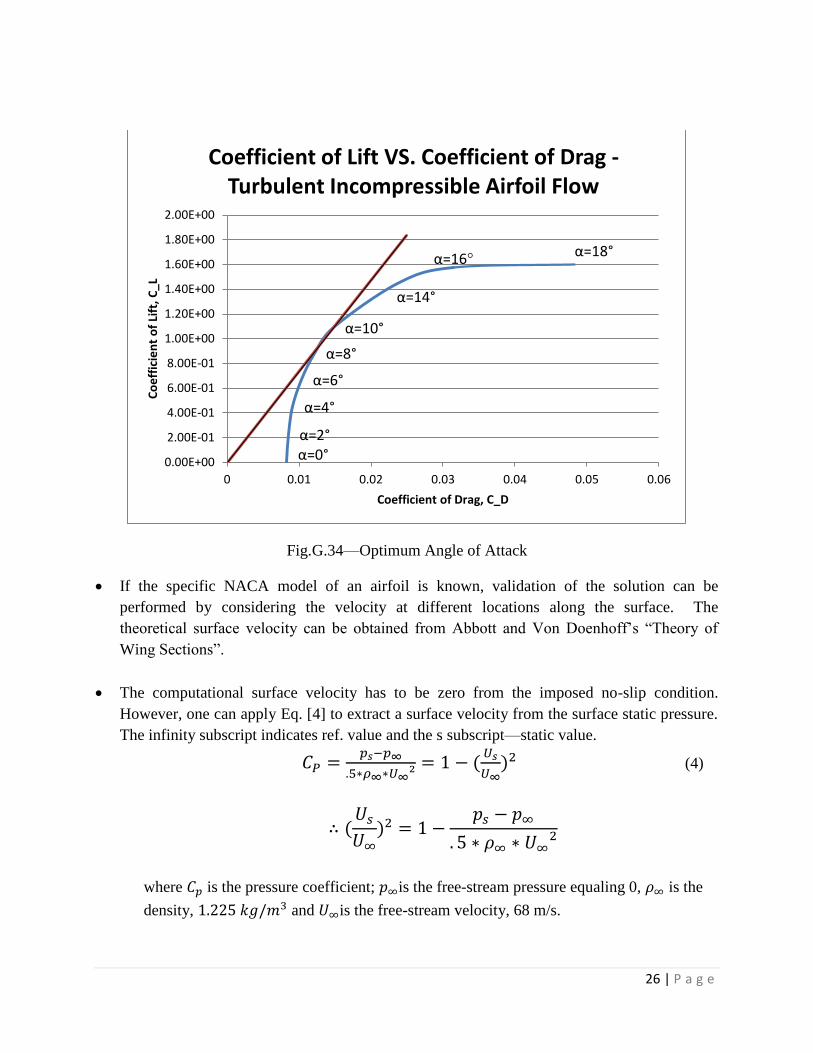
The most efficient angle of attack is represented by the highest L/D ratio. Graphically the

results are shown in Figs.G.33-34. It is evident the most efficient angle of attack for the

turbulent incompressible case [with the energy equation turned off] is around 10 degrees.

Stall occurs around an angle of attack of 18 degrees.

Angle of Attack,

-10 -5 0 5 10 15 20

Lift to

Dra

g R

atio

, C

L/C

D

-80

-60

-40

-20

0

20

40

60

80

Turb. Icompr. Flow, Energy Off

Fig.G.33—Determination of Most Optimum Angle of Attack

26 | P a g e

Fig.G.34—Optimum Angle of Attack

If the specific NACA model of an airfoil is known, validation of the solution can be

performed by considering the velocity at different locations along the surface. The

theoretical surface velocity can be obtained from Abbott and Von Doenhoff’s ―Theory of

Wing Sections‖.

The computational surface velocity has to be zero from the imposed no-slip condition.

However, one can apply Eq. [4] to extract a surface velocity from the surface static pressure.

The infinity subscript indicates ref. value and the s subscript—static value.

(4)

∞

∞

∞ ∞

where is the pressure coefficient; ∞is the free-stream pressure equaling 0, ∞ is the

density, and ∞is the free-stream velocity, 68 m/s.

α=0°

α=2°

α=4°

α=6°

α=8°

α=10°

α=18°

α=14°

α=16°

0.00E+00

2.00E-01

4.00E-01

6.00E-01

8.00E-01

1.00E+00

1.20E+00

1.40E+00

1.60E+00

1.80E+00

2.00E+00

0 0.01 0.02 0.03 0.04 0.05 0.06

Co

eff

icie

nt

of

Lift

, C_L

Coefficient of Drag, C_D

Coefficient of Lift VS. Coefficient of Drag -Turbulent Incompressible Airfoil Flow

27 | P a g e

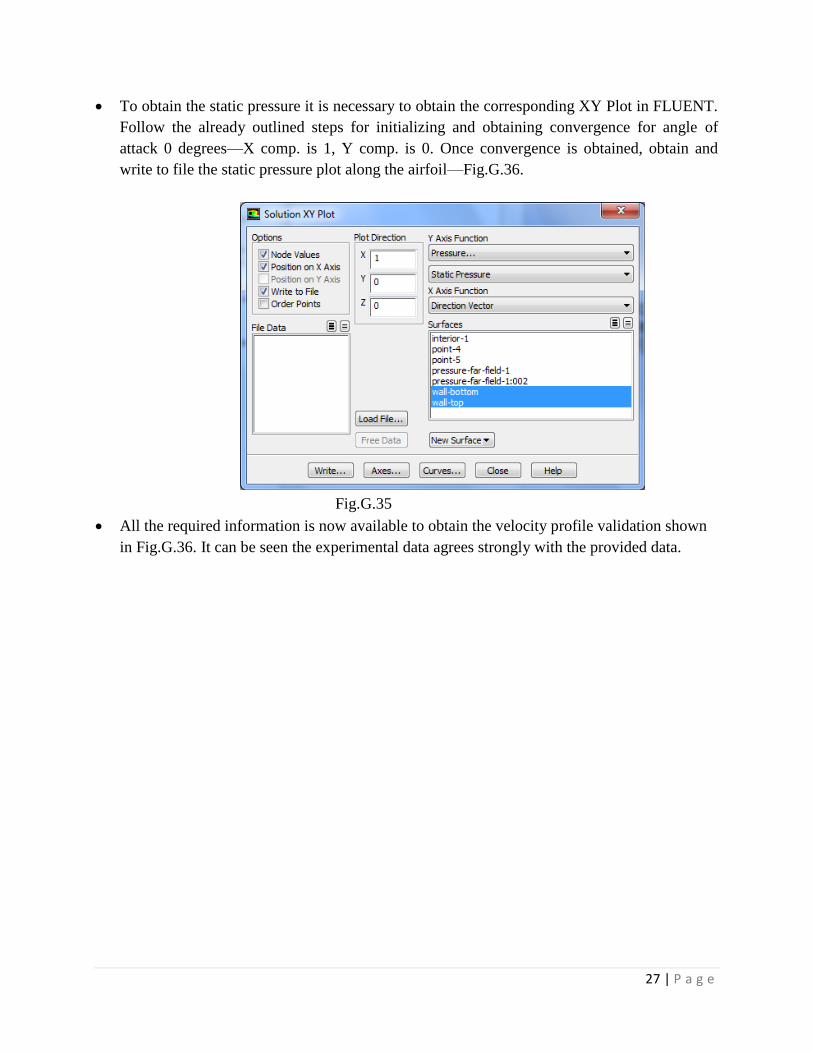
To obtain the static pressure it is necessary to obtain the corresponding XY Plot in FLUENT.

Follow the already outlined steps for initializing and obtaining convergence for angle of

attack 0 degrees—X comp. is 1, Y comp. is 0. Once convergence is obtained, obtain and

write to file the static pressure plot along the airfoil—Fig.G.36.

Fig.G.35

All the required information is now available to obtain the velocity profile validation shown

in Fig.G.36. It can be seen the experimental data agrees strongly with the provided data.

28 | P a g e

NACA0012, =0

Axial Position, x/c

0.0 0.2 0.4 0.6 0.8 1.0

Surf

ace V

elo

city, [u/U

] 2

0.0

0.2

0.4

0.6

0.8

1.0

1.2

1.4

1.6

Abbott & Von Doenhoff

Incomp., Turb., No Energy

Incomp., Turb. Energy

Fig.G.36