Module D: Laminar Flow over a Flat Plate

Summary…..……………………………………………….

Problem Statement…………………………………………

Geometry and Mesh Creation………………………………

Problem Setup………………………………………………

Solution…………………………………………………….

Results

Validation……………………...………...………………...

Mesh Refinement………………………………………..…

Summary

This ANSYS FLUENT tutorial is to leads a user through the basic steps simulating flow over a flat plate.

The steps include setting initial and boundary conditions inputs, setting reference values and residuals and

making sure a converged solution is obtained upon initialization of the problem. Next, the obtained results

are validated against either theoretical or empirical data. This tutorial will focus on two distinct cases. The

first case involves laminar flow without heat transfer, while the second case focuses on laminar flow with

heat transfer. By completing this tutorial the user gains more experience in geometry and mesh creation

as well as proper problem setup in FLUENT. Finally the user is exposed to methods of simulation

validation to ensure the obtained the result are reasonable.

Problem Statement:

Consider the flat plate for which the geometry and the corresponding mesh were created in

ANSYS Workbench:

Fig.D.1

Symmetry

Wall

Outlet Inlet Width,w

Length,L

Air

The inlet velocity, , L=1.0m, w=0.5 m. Also let us assume the density, of the

fluid to be

⁄ and the dynamic viscosity, to be 0.0001

⁄ . The corresponding

Reynolds number can be calculated:

(1)

(

⁄ )

⁄

For an external flow over a flat plate such as the one under consideration, the critical value for the

Reynolds number ( ) after which the flow is to be considered turbulent is 500,000. Hence we

are dealing with laminar flow. Both laminar and turbulent flow can exist along the flat plate and if

the plate is sufficiently large the flow can be assumed to be turbulent.

Geometry Creation:

Start ANSYS Workbench. In Toolbox select the Mesh component system under

Component Systems. Drag it to the Project Schematic. The system can be renamed by

double clicking on the default text ―Mesh‖.

Fig.C.2

Double click the text to rename

the system.

Select the Mesh component system

and drag it to the Project Schematic.

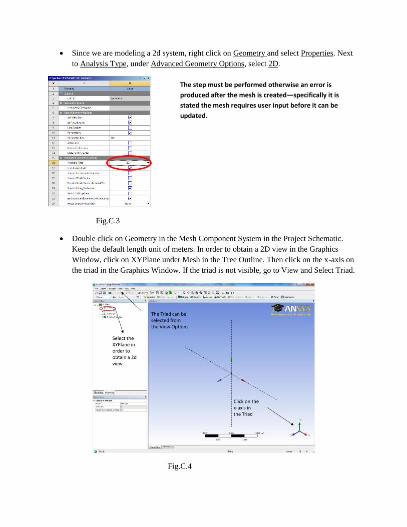
Since we are modeling a 2d system, right click on Geometry and select Properties. Next

to Analysis Type, under Advanced Geometry Options, select 2D.

Fig.C.3

Double click on Geometry in the Mesh Component System in the Project Schematic.

Keep the default length unit of meters. In order to obtain a 2D view in the Graphics

Window, click on XYPlane under Mesh in the Tree Outline. Then click on the x-axis on

the triad in the Graphics Window. If the triad is not visible, go to View and Select Triad.

Fig.C.4

Click on the x-axis in the Triad

The Triad can be selected from the View Options

Select the XYPlane in order to obtain a 2d view

The step must be performed otherwise an error is

produced after the mesh is created—specifically it is

stated the mesh requires user input before it can be

updated.

Next the rectangle representing the flat plate is to be sketched. Select Sketching in the

Tree Outline. Select Rectangle from the Drawing Options. The rectangle is to be drawn

fixed at the origin therefore make sure the letter P is visible in the Graphics window upon

placing the drawing pencil at the origin.

Fig.C.5

Next drag the drawing pencil in the Graphics window from the origin to 1st Quadrant.

The dimensions will be specified later so for now they can be arbitrary.

The “P” means the

shape to be drawn is

fixed at the origin

Select

Sketching to

draw the flat

plate

Select the

rectangle

shape

Fig.C.6

Let us model a flat plate of length 1 meter and width 0.5 meters. Select Dimensions from

under Sketching Toolboxes. Keep the default selection of General. Select one of the

vertical edges in the Graphics Window. By moving away from the edge a ruler can be

seen and by clicking once it will become fixed. In the lower left hand side under Details

View the vertical dimension can be specified. Type 0.5 under Dimensions.

Fig.C.7

Select a

vertical edge

Specify the

vertical

dimensions

Repeat the same procedure, this time select one of the horizontal edges and under details

view specify a length of 1 meter.

Fig.C.8

Fig.C.9

The shape can be manipulated to fit on screen by right clicking zoom to fit in the graphics

window. Then pan or box zoom options can be used to manually adjust drawing view.

Select Modeling from under Sketching Toolboxes. Under XYPlane, select created sketch.

Select Surfaces from Sketches from under Concept. Next to Base Objects under Details

View, select Apply. The order is irrelevant: the Surfaces from Sketches can be selected

first, then the sketch can be selected under XYPlance and then Apply can be clicked.

Finally click Generate to create the body.

Fig.C.10

Fig.C.11

Click on Generate

to create the body

Can be inspected to

see whether body is

created

You can exit the DesignModeler and the geometry will be automatically saved. A

checkmark next to geometry means no issues were found by Workbench. We can now

proceed with meshing the plate.

Mesh Creation:

Double click on Mesh in Project Schematic. In Meshing Options window that appears

upon loading Meshing, select CFD for the Physics Preference. Keep the other defaults.

Press OK.

Under Units, verify that metric units (m, kg, N) are used. Make sure the Advanced Size

Function under Mesh, Sizing is off since we are to manually specify the mesh element

size.

Fig.C.12

For such a basic shape like a rectangle we would like to create a structured mesh meaning

the mesh is to consist of rectangles which are to exhibit a pronounced pattern. Therefore

we have to make sure opposite edges correspond with each other. The way to do this is to

select Mapped Face Meshing under Mesh Control. Select the rectangle in the graphics

window (it should turn green). Click Apply (the rectangle should turn blue now).

Fig.C.13

Under Details, next to Method, the Option Quadrilaterals signifies the mesh is to consist

of rectangular elements.

The structured mesh that is to be created is of size 60X50 meaning there will be 60 mesh

(grid) divisions in the y-dir. and 50 divisions in the x-dir.

Let us mesh the horizontal edges first. Select Sizing under Mesh Control. Select the edge

cube and then select both the upper and lower horizontal edges (hold the ctrl button to

select more than one edge). Select Apply next to Geometry under Details of Sizing.

Under Definition, next to Type select Number of Divisions. Specify 50 divisions and

change the Behavior from Soft to Hard in order to overwrite the default sizing functions

used by Workbench.

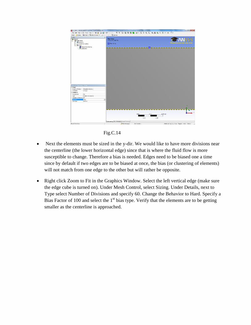
Fig.C.14

Next the elements must be sized in the y-dir. We would like to have more divisions near

the centerline (the lower horizontal edge) since that is where the fluid flow is more

susceptible to change. Therefore a bias is needed. Edges need to be biased one a time

since by default if two edges are to be biased at once, the bias (or clustering of elements)

will not match from one edge to the other but will rather be opposite.

Right click Zoom to Fit in the Graphics Window. Select the left vertical edge (make sure

the edge cube is turned on). Under Mesh Control, select Sizing. Under Details, next to

Type select Number of Divisions and specify 60. Change the Behavior to Hard. Specify a

Bias Factor of 100 and select the 1st bias type. Verify that the elements are to be getting

smaller as the centerline is approached.

Fig.C.15

Repeat the same procedure for the other vertical edge. This time the 2nd

Bias type must be

selected, everything else remains the same as with the previously manipulated vertical

edge.

Fig.C.16

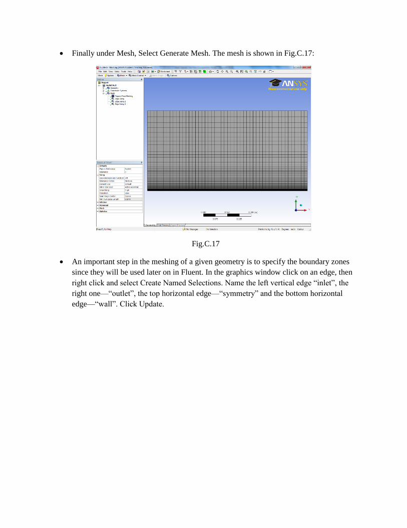
Finally under Mesh, Select Generate Mesh. The mesh is shown in Fig.C.17:

Fig.C.17

An important step in the meshing of a given geometry is to specify the boundary zones

since they will be used later on in Fluent. In the graphics window click on an edge, then

right click and select Create Named Selections. Name the left vertical edge ―inlet‖, the

right one—―outlet‖, the top horizontal edge—―symmetry‖ and the bottom horizontal

edge—―wall‖. Click Update.

Fig.C.18

The mesh can be exported and then loaded in ANSYS Fluent by saving it as a .msh file.

This can be done by selecting Export under File. Save is as a Fluent input file (.msh).

You can now exit Meshing. A checkmark should appear next to Mesh in the Workbench

Project Schematic indicating no problems were found with the created Mesh. Save the

Project to make sure the Geometry and Mesh can be manipulated further if need be.

Geometry and Mesh Creation:

Refer to the Flat Plate—Mesh tutorial (Appendix C) for an in-depth walkthrough of the

flat plate geometry and meshing creation. The mesh to be used in ANSYS FLUENT

should look like the one in Fig. X.

Fig.D.2

Problem Setup:

Open ANSYS FLUENT. In the FLUENT Launcher, make sure the Dimension is

specified to be 2D. For better accuracy under Options select Double Precision (note more

memory will be used). Keep the rest of the defaults. For better convenience, select the

folder in which the flat plate mesh has been saved as the working directory. Press OK.

Fig.D.3

Under Main—File—Read, Select Mesh and open the created Flat Plate Mesh.

Fig.D.4

Problem Setup--General:

In Scale, verify the dimensions as stated in the problem statement and make sure the length units

are meters.

Fig.D.5

Select Check—any errors will be reported. Make sure the minimum volume is positive in order to

make sure a solution can be calculated.

In Display, make sure all surfaces are selected.

Fig.D.6

Keep the defaults in the Solver.

Fig.D.7

Problem Setup--Models:

Keep the defaults in Models. Laminar flow is to be analyzed based on the computed Reynolds

number and since no heat transfer is to be taken into consideration, the energy equation should be

off.

Fig.D.8

Problem Setup--Materials:

In Materials, under Fluid double click on Air. Specify the density and viscosity as given in the

problem statement. The name of the fluid can be changed in order to more accurately express the

input values. Press Change/Create.

Fig.D.9

Problem Setup—Boundary Conditions:

Five zones should exist as the boundary condition zones—the inlet, outlet, centerline and farfield

(as specified in Workbench) as well as the interior of the body. We have to make sure the zones

are of the correct type:

Table D.1

Zone Type

Inlet Velocity-inlet

Outlet Pressure-outlet

Symmetry Symmetry

Wall Wall

Interior-surface_body Interior

Fig.D.10

Problem Setup—Boundary Conditions:

Double click on inlet to specify in the inlet velocity magnitude which is given as 1.0 m/s. Press

OK.

Fig.D.11

Make sure the outlet gauge pressure, in the outlet zone is 0 Pa—since the gauge pressure at the

outlet is the difference of the operating pressure, 1 atm, and the absolute pressure, 1 atm.

Fig.D.12

Under Operating Conditions, verify that the Operating Pressure is 101,325 Pa (1 atm).

Fig.D.13

Problem Setup—Reference Values:

Reference values have to be specified since they will be needed for postprocessing, i.e. skin

friction (Fanning friction). In reference values, under compute from, select the inlet. Verify the

reference values match those that were input as initial and boundary conditions (inlet velocity,

density, viscosity).

Fig.D.14

Solution—Solution Methods:

In Solution—Solution Methods, under Spatial Discretization make sure Momentum is of type

Second Order Upwind. While the convergence will not be as robust as when the First Order

Upwind, the accuracy will be better for the type specified.

Fig.D.15

Solution—Monitors:

In Monitors, under Residuals, click Edit. It is important to specify an absolute convergence

criterion for each residual equation. Doing so will ensure that convergence is achieved, upon

reaching the specified value, for all governing equations on which the solution depends. Set the

absolute criteria to 1e-06 for the three equations. Make sure under Options both Print to Console

and Plot are checked. Enter OK.

Fig.D.16

Solution Initialization:

Before a solution can be calculated the problem must first be initialized. Under Solution

Initialization, under compute from select the inlet. Make sure the x velocity is 1 m/s as given and

the y velocity is set to 0. Select Initialize.

Fig.D.17

Solution—Run Calculation:

Set the number of iterations to 500. Press Calculate. While it can be seen the solution is

converging the absolute convergence criterion that was specified has not been reached. The

calculations can be restarted without having to initialize the problem again. Simply enter the

additional iterations that are to be computed (let‘s keep the 500 iterations that were previously

specified). Enter Calculate again. Upon reaching the specified convergence value the iterations

stop. It can be seen convergence is achieved at the 665th iteration.

Graph D.1—Convergence Residuals

Results:

Let us graph the skin fraction coefficient as well as the velocity profile in the y-direction.

Afterwards the obtained results will be validated against a known solution.

In Results—Plots select XY Plot. Double click it. Make sure Position on X axis is selected as

well as Node Values. In Plot Direction make sure x=1 and y=0 (x will thus become the abscissa

or horizontal coordinate). Select Wall Fluxes from under Y Axis Function and choose Skin

Friction Coefficient. Select the centerline surface. Click Plot.

Fig.D.18

Graph D.2—Skin Friction Coefficient

The graph can be saved as a picture by selecting Save Picture under Main Menu-- File. The

different saving options are explained when Help is pressed. Usually the TIFF or JPEG formats

are best.

The graph can be manipulated –by going back to the XY Plot and selecting curves, the markers

can be replaced by a line with a user chosen color and weight.

Fig.D.19

The graph can be further enhanced by manipulating the y-axis values. By selecting Axes, in the

number format the type can be changed from exponential to float. Make sure to click apply after a

change has been made for a particular axis. The graph produced as a result is shown below:

Graph D.3

Fig.D.20

The plot can be saved by clicking on Write to File

in the Solution XY Plot window. Press Write

afterwards and save the plot as a .xy file. The .xy

file can be then opened in Excel where

dimensional analysis for validation purposes can

be performed. This will be demonstrated later.

Fig.D.21

Results—Velocity Profile XYPlot:

In the Solution XY Plot deselect Position on X Axis and select Position on Y axis since we are to

plot the velocity profile in the y-direction. In Plot Direction set x=0 and y=1. Under X Axis

Function select Velocity and specify X Velocity. Deselect the center_line surface by clicking it

again and select the outlet one. Click Plot.

Fig.D.22

Graph D.4—Velocity Profile

Save the Plot so it can be analyzed later on in Excel.

Results—Graphics and Animations:

The velocity profile can be observed along the axial distance of the flat plate. In Graphics and

Animations, under Graphics double click on Vectors. Set the scale to 0.5 and press display. The

colormap can be moved for better visual representation. That can be done by selecting Options

under Graphics and Animations and by adjusting the colormap alignment under layout. Select

Bottom and click Apply. The colormap scale can be manipulated by selecting colormap under

Graphics and Animations and by changing the type from exponential to general. Press Apply.

Fig.D.23 Fig.D.24

Fig.D.25—Velocity Vectors

Results—Graphics and Animations:

The pressure coefficient can also be visually inspected along the flat plate. In Results—Graphics

and Animations, double click on Contours. Make sure under Options, Filled is checked. Set the

levels to 90 and press display.

Fig.D.26 Fig.D.27

The colormap may have to be adjusted in order to prevent the values from becoming too

clustered. Manipulate the skip option until satisfactory colormap appearance is obtained.

Fig.D.28—Pressure Coefficient Contours

Velocity Validation Based on the Similarity Variable:

After results have been obtained it is critical to validate them against known data in order to make

sure the experimental data obtained from FLUENT makes sense.

The Navier-Stokes equations which are solved to yield the obtained data can be simplified for

boundary layer flow analysis. It can be assumed that the boundary layer is thin and the fluid flow

is primarily parallel to the plate. Hence:

(2)

(3)

H. Blasius, one of Prandtl‘s students was able to solve those equations for flat plate parallel to the

flow. By introducing the dimensionless parameter (the similarity variable) the partial

differential equations are reduced to an ordinary differential equation.

√

(4)

where U is the inlet velocity and is the kinematic viscosity,

The convenience of validating the boundary layer velocity profile in terms of the similarity

variable is that the boundary layer velocity profiles (which depends both on x and y) at any point

along the plate will overlap one another and can be analyzed versus the empirical Blasius

correlation. The procedure of accomplishing this is now explained.

Open FLUENT and load the original flat plate mesh—50X60 grid biased towards the wall

surface(lower horizontal edge). Repeat the steps outlined in this tutorial to obtain convergence.

Another way of doing this is to create a FLUENT Flow system in Workbench through which

FLUENT can be started in the Setup step. The system can be duplicated and changes can be made

(mesh) and updates can automatically be done which eliminates the need to go through the

problem setup in FLUENT for each change made in the mesh (ref. Turbulent Pipe Flow tutorial).

However the user can become more familiar with the software by going through the process

again.

Let us now display the velocity profile at not only the outlet but at three other specific points

along the plate. To do that, lines at those points must be created. Go to Surface—Line/Rake.

Make sure the Line Tool is checked. Specify the following points to create the line— . Specify a name that can easily be recognized and press create.

Proceed to create two more lines—at 0.6m and at 0.8m along the plate.

Fig.D.29

Next go to Results—Plots-XY Plot. Proceed to obtain the boundary layer velocity profile like

before. However this time select not only the outlet surface but the three created lines as well.

The result is displayed in Graph D.6:

Graph D.5—Axial Velocity Plot in FLUENT

Save the XY plot so the data can be manipulated in Excel to obtain the similarity variable.

Open Excel and load the XY plot. Let us first obtain the Blasius correlation. Refering to

Fundametals of Fluid Mechanics by Munson and etc. the following correlation is provided:

Table D.1—The Blasius Solution for Laminar Flow along a Flat Plate

⁄ ⁄

0 0

0.4 0.1328

0.8 0.2647

1.2 0.3938

1.6 0.5168

2.0 0.6298

2.4 0.7290

2.8 0.8115

3.2 0.8761

3.6 0.9233

4.0 0.9555

4.4 0.9759

4.8 0.9878

5.0 0.9916

5.2 0.9943

5.6 0.9975

6.0 0.9990

For the imported experimental data the u/U parameters can simply be created by dividing each

velocity entry by the maximum value. The similarity variable can be then be created at each of

the data points for which the profile was obtained in FLUENT (at x=0.4, x=0.6, x=1, etc); U is

given as 1 m/s and the kinematic viscosity ends up equalling the dynamic one since the density is

stated as 1.0 kg/ ; y varies since the velocity data is given at various points along the vertical of

the plate. Graph D.6 can be thus obtained:

Fluent, Laminar, 50 x 60 Grid

Velocity, u/U

0.0 0.2 0.4 0.6 0.8 1.0 1.2

Sim

ilarity

Variable

,

0

1

2

3

4

5

6

Blasius

Fluent, x/L=0.6

Fluent, x/L=0.8

Fluent, x/L=1.0

Graph D.6—Boundary Layer Profile, FLUENT data for Re=10,000

As it can be seen the obtained experimental data by FLUENT agrees very closely with the Blasius

correlation. Also notice how the boundary layer profiles at each specified points along the plate

lay on top of each other as they should. Only one curve is necessary to describe the velocity at

any point in the boundary layer.

Another way of obtaining validation is if the Blasius correlation is plotted in the y-dir. The

Blasius data needed is provided in the tutorial and validation is performed for various meshes of

the flat plate to determine the most accurate one.

First the original mesh is plotted against the Blasius correlation in Excel. For the experimental

data u/U and y/Y are obtained in the same fashion as discussed previously for dimensionless data

validation (ref. to Nikuradse validation for Turbulent flow in cylindrical pipe module, Appendix

B). Basically the saved .xy plot can be opened in Excel and each entry for the velocity ‗u‘ is

divided by the maximum value for the velocity U. Same is repeated for y.

The experimental data closely agrees with the Blasius solution—Graph D.7.

Graph D.7

The skin friction coefficient data given by FLUENT is validated against the Blasius Solution—

Eq. [5].

√ (5)

(6)

where x is the distance along the plate, in meters

Ref. to Appendix A and B for in-depth discussion of skin friction coefficient.

The validation can be observed in Graph D.8.

0

0.02

0.04

0.06

0.08

0.1

0.12

0.14

0.16

0.18

0.2

0 0.2 0.4 0.6 0.8 1 1.2

y/Y

u/U

Y-axis Velocity Profile Correlation

60X50 Grid, Re=1e04

Blasius Soln

Axial Distance, x/L

0.0 0.2 0.4 0.6 0.8 1.0

Skin

Fri

ction C

oe

ffic

ient, C

f x R

ex

1/2

0.4

0.6

0.8

1.0

1.2

Fluent, Re=10,000

Blasius

Graph D.8—Skin Friction Coefficient Validation

Mesh Refinement:

Refine the flat plate mesh and see if the solution becomes more accurate. This can be done in

three ways—with unstructured mesh, with a 60X200 structured mesh and with a structured

60X50 mesh which is to have a different bias type.

Open the Workbench project used to create mesh (ref. to the Flat Plate—Meshing tutorial). Make

three copies of the existing Mesh by right clicking on mesh and selecting Duplicate. Rename

three created mesh copies ―Unstructured 60X50 Mesh‖, ―60X200 Structured Mesh‖, and ―60X50

opposite bias‖. The Project Schematic should look like the one provided in Fig.D.30:

Fig.D.30

In the Project Schematic, double click on the 60X200 Mesh. Under Mesh in the Outline, select

the edge sizing for the horizontal edges and change the number of divisions from 50 to 200.

Everything else remains absolutely the same. Click Update and export the mesh by selecting

Main Menu—File,Export. Save the mesh as a .msh file. Close the Meshing.

Fig.D.31

Fig.D.32

Open the Unstructured Mesh System in the Project Schematic by double clicking Mesh. In the

Outline delete the Mapped Face Meshing sizing. Click Update. Notice the lack of pattern in the

mesh. Again save the newly created mesh and exit Meshing.

Fig.D.33

Finally let us select a different bias type. Double click on Mesh in Different Bias Type System.

Change bias for the two vertical edges so that there are more elements near the farfield boundary

zone rather than near the centerline zone. Click Update and save the mesh. Exit Meshing.

Fig.D.34

Open FLUENT and for each of the three refined meshes obtain the velocity profile in the y-dir.

xy plot in the same manner as it was obtained for the original mesh. Do not forget to set the

reference values from the inlet as well as to initialize and obtain the convergence. Notice how for

the 60X200 Mesh convergence is obtained after more iteration, since there are more elements in

the mesh.

The xy plots can be opened in Excel and then dimensional analysis can be performed for the

velocity profile in the y-direction. The x-axis signifies u/U, each entry for the velocity is divided

by the maximum velocity for the corresponding mesh while the y-axis displays y/Y which is

obtained by dividing each entry for the distance by the total distance in the y-direction for the flat

plate which is 0.5 meters.

Velocity, u/U

0.0 0.2 0.4 0.6 0.8 1.0 1.2

Ve

rtic

al D

ista

nce

, y/Y

0.00

0.05

0.10

0.15

0.20

0.25

0.30

Blasius

60 x 50, unstructured

60 x 200

Graph D.9

It can be observed in Graph D.9 that the best results are obtained with the 60X50 Unstructured

Mesh (Fig.D.33) and the 60X200 Structured Mesh (Fig.D.32). However it is advisable, when

dealing with problems with simple geometry like the one in this tutorial, to use structured mesh.

Let us now change the geometry, specifically alter the farfield boundary and determine if the

obtained data is more accurate when it is validated against the similarity variable.

Fig.D.35

The new geometry created reflects the farfield boundary is at 15 degree angle with the horizontal.

The shape is created not from sketch but rather the coordinates are specified by plotting points

and then connecting the points to form edges (Concept—Edges from Points). Finally the surface

created is from edges rather than from a sketch (Concept—Surfaces from Edges). Make sure the

corresponding filter is selected—filter by points for point selection to create the four edges, filter

by edges to select the edges to form a surface.

Everything else remains the same—the length of the plate is still 1 meter and the material

properties will stay the same as well. Refer to the meshing tutorial for the flat plate for any issues

arising for the new plate geometry. Next the corresponding mesh is created:

Fig.D.36

The mesh is created in the same way as before. The mesh for the new plate geometry is 50X60

(axial X vertical) with bias of 100 towards the wall surface. Export the mesh into FLUENT.

Obtain converge in the familiar manner and create 2 lines—1 at x=0.6 and another one at x=0.8.

Care must be exercised when creating the lines since the farfield boundary is not constant

anymore—it is linear:

Fig.D.37

Hence the coordinates for the 2 lines to be created are:

Plot boundary layer velocity profile at the outlet and the two created lines and save the xy plot.

0.5 m

y

0.6 m

1.0 m

y’’ y’

0.8 m

Outlet

Wall

Farfield

Inlet

Graph D.10

Velocity, u/U

0.0 0.2 0.4 0.6 0.8 1.0

Sim

ilari

ty V

ari

ab

le,

0

1

2

3

4

5

6

Blasius

50 x 60, x/L=0.6

50 x 60, x/L=0.8

50 x 60, x/L=1.0 [outlet]

Graph D.11

From the dimensional analysis, it seems the further one gets away from the outlet the more

accurate the solution gets. However, regardless of where on the plate the profile is analyzed, the

experimental curves should overlap each other. One explanation is that the discrepancy seen here

is due to the farfield boundary that was changed.