MODULE A: ECOCLASSIFICATION AND ECOSTATUS DETERMINATION · PDF fileriver ecoclassification...
59
Transcript of MODULE A: ECOCLASSIFICATION AND ECOSTATUS DETERMINATION · PDF fileriver ecoclassification...

RIVER ECOCLASSIFICATION MANUAL FOR ECOSTATUS DETERMINATION
(Version 2)
MODULE A: ECOCLASSIFICATION AND ECOSTATUS
DETERMINATION
CJ KLEYNHANS Department of Water Affairs & Forestry, Resource Quality Services, Pretoria MD LOUW Water for Africa, Pretoria

Module A: EcoStatus March 2007 Page Ai
DOCUMENT REFERENCE
Kleynhans CJ, Louw MD. 2007. Module A: EcoClassification and EcoStatus determination in River EcoClassification: Manual for EcoStatus Determination (version 2). Joint Water Research Commission and Department of Water Affairs and Forestry report. WRC Report No.
ACKNOWLEDGEMENTS
All those that have ever been involved in the process of determining PES, Future Desired state, Environmental Management Class, Recommended Ecological Reserve and any other terminology that bears relevance to ecological state.
Module A: EcoStatus March 2007 Page Aii
STRUCTURE OF THE MANUAL
The manual consists of the following modules: • MODULE A: ECOCLASSIFICATION AND ECOSTATUS MODELS
• MODULE B: GEOMORPHOLOGICAL DRIVER ASSESSMENT INDEX (GAI) • MODULE C: PHYSICO-CHEMICAL DRIVER ASSESSMENT INDEX (PAI) • MODULE D: FISH RESPONSE ASSESSMENT INDEX (FRAI) • MODULE E: MACRO-INVERTEBRATE RESPONSE ASSESSMENT INDEX
(MIRAI) • MODULE F: RIPARIAN VEGETATION RESPONSE ASSESSMENT INDEX
(VEGRAI) • MODULE G: INDEX OF HABITAT INTEGRITY This is module A which provides the background to and scientific rationale for the EcoClassification and EcoStatus processes. It also provides the process of determining the EcoStatus and explains the different EcoStatus models used for different levels of assessment.
PURPOSE OF THE MANUAL : MODULE A
§ Describe the concepts on which the EcoStatus approach is based. § Establish and demonstrate its application in terms of EcoClassification as it
relates to Ecological Water Requirement (EWR) determination (as part of the Ecological Reserve), Ecological Reserve monitoring, and the River Health Programme.
§ Provide guidance to specialists and Environmental Water Requirement and River Health Programme technical coordinators in the use of the EcoStatus rule-based models
WHO SHOULD APPLY THESE MODELS?
An experienced river ecologist. NOTE: It is strongly recommended that the user participates in training courses and/or contact the authors of this manual when applying the models
The manual is in two sections. The first section provides an introduction, background, general process and the scientific rationale of the EcoClassification process.
Module A: EcoStatus March 2007 Page Aiii
FIRST SECTION OF THE MANUAL
Chapter 1: EcoClassification: Contains the background, introduction and a description of the EcoClassification process Chapter 2: EcoStatus Introduction: Provides the background, introduction, scientific rationale and concepts of the EcoStatus.
The second section is the 'how to' section, that is, the more traditional manual part.
SECOND SECTION OF THE MANUAL Chapter 3: EcoStatus determination: Contains the explanation of the various EcoStatus models and the use there-of. Chapter 4: Guidance in the use of the EcoStatus Level 4 process: Provides a step by step guidance in the application of the EcoStatus models with specific reference to timing of specialist input.

Module A: EcoStatus March 2007 Page Aiv
EXECUTIVE SUMMARY
1. ECOCLASSIFICATION EcoClassification - the term used for the Ecological Classification process - refers to the determination and categorisation of the Present Ecological State (PES; health or integrity) of various biophysical attributes of rivers relative the natural or close to the natural reference condition. The purpose of the EcoClassification process is to gain insights and understanding into the causes and sources of the deviation of the PES of biophysical attributes from the reference condition. This provides the information needed to derive desirable and attainable future ecological objectives for the river. The steps followed in the EcoClassification process are as follows: • Determine reference conditions for each component. • Determine the Present Ecological State for each component as well as for the
EcoStatus. The EcoStatus refers to the integration of physical changes by the biota and as reflected by biological responses.
• Determine the trend (i.e., moving towards or away from the reference condition) for each component as well as for the EcoStatus.
• Determine causes for the PES and whether these are flow or non-flow related.
• Determine the Ecological Importance and Sensitivity (EIS) of the biota and habitat.
• Considering the PES and the EIS, suggest a realistic and practically attainable Recommended Ecological Category (REC) for each component as well as for the EcoStatus.
• Determine alternative Ecological Categories (ECs) for each component as well as for the EcoStatus for the purposes of providing various scenarios
The EcoClassification process is an integral part of the Ecological Reserve determination method and of any Environmental Flow Requirement method. Flows and water quality conditions cannot be recommended without information on the predicted resulting state, the Ecological Category. Biological monitoring for the River Health Programme (RHP) also uses the EcoClassification process to assess biological response data in terms of the severity of biophysical changes. However, the RHP focuses primarily on biological responses as an indicator of ecosystem health, with only a general assessment of the cause-and-effect relationship between the drivers and the biological responses. 2. ECOSTATUS INTRODUCTION The EcoStatus is defined as
Module A: EcoStatus March 2007 Page Av
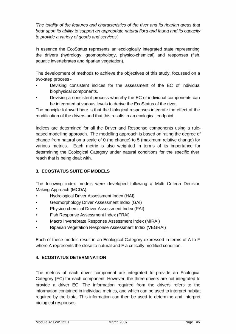
'The totality of the features and characteristics of the river and its riparian areas that bear upon its ability to support an appropriate natural flora and fauna and its capacity to provide a variety of goods and services'. In essence the EcoStatus represents an ecologically integrated state representing the drivers (hydrology, geomorphology, physico-chemical) and responses (fish, aquatic invertebrates and riparian vegetation). The development of methods to achieve the objectives of this study, focussed on a two-step process - • Devising consistent indices for the assessment of the EC of individual
biophysical components. • Devising a consistent process whereby the EC of individual components can
be integrated at various levels to derive the EcoStatus of the river. The principle followed here is that the biological responses integrate the effect of the modification of the drivers and that this results in an ecological endpoint. Indices are determined for all the Driver and Response components using a rule-based modelling approach. The modelling approach is based on rating the degree of change from natural on a scale of 0 (no change) to 5 (maximum relative change) for various metrics. Each metric is also weighted in terms of its importance for determining the Ecological Category under natural conditions for the specific river reach that is being dealt with.
3. ECOSTATUS SUITE OF MODELS The following index models were developed following a Multi Criteria Decision Making Approach (MCDA). • Hydrological Driver Assessment Index (HAI) • Geomorphology Driver Assessment Index (GAI) • Physico-chemical Driver Assessment Index (PAI) • Fish Response Assessment Index (FRAI) • Macro Invertebrate Response Assessment Index (MIRAI) • Riparian Vegetation Response Assessment Index (VEGRAI) Each of these models result in an Ecological Category expressed in terms of A to F where A represents the close to natural and F a critically modified condition. 4. ECOSTATUS DETERMINATION
The metrics of each driver component are integrated to provide an Ecological Category (EC) for each component. However, the three drivers are not integrated to provide a driver EC. The information required from the drivers refers to the information contained in individual metrics, and which can be used to interpret habitat required by the biota. This information can then be used to determine and interpret biological responses.

Module A: EcoStatus March 2007 Page Avi
The fish and invertebrate response indices are interpreted to determine an Instream Ecological Category using the Instream Response Model. The purpose of this model is to integrate the EC information on the fish and invertebrate responses to provide the instream EC. The basis of this determination is the consideration of the indicator value of the two biological groups to provide information on - • Fish: Diversity of species with different requirements for flow, cover, velocity-
depth classes and modified physico-chemical conditions of the water column. • Invertebrates: Diversity of taxa with different requirements for biotopes,
velocity and modified physico-chemical conditions. Due to time and funding constraints, various levels of Reserve determinations can be undertaken. Each of these relates to an Ecological Water Requirement (EWR) method with an appropriate level of detail and EcoClassification process. The EcoClassification process, and specifically the detail and effort required for assessing the metrics, varies according to the different levels. The process to determine the EcoStatus also differs on the basis of different levels of information. There are five EcoStatus levels and they are linked to the different levels of Ecological Reserve determination as follows: • Desktop Reserve method ? Desktop EcoStatus level. • Rapid I Ecological Reserve method ? EcoStatus Level 1. • Rapid II Ecological Reserve methods ? EcoStatus Level 2 • Rapid III Ecological Reserve methods ? EcoStatus Level 3 • Intermediate and Comprehensive Reserve methods ? EcoStatus Level 4 These five levels of EcoStatus determination are associated with an increase in the level of detail required to execute them. As the EcoStatus levels become less complex, less-complex tools must be used (such as the Index of Habitat Integrity). The manual explains these different tools, how they work and when they should be applied.

Module A: EcoStatus March 2007 Page Avii
ABBREVIATIONS
ASPT Average Score Per Taxon DWAF Department of Water Affairs and Forestry EC Ecological Category EcoSpecs Ecological Specifications EIS Ecological Importance and Sensitivity ER Ecological Reserve EWR Ecological Water Requirements FAII Fish Assemblage Integrity Index FHS Fish Habitat Segment FRAI Fish Response Assessment Index GAI Geomorphology Driver Assessment Index HAI Hydrology Driver Assessment Index IHI Index of Habitat Integrity ISP Internal Strategic Perspective IFR Instream Flow Requirements MCDA Multi-Criteria Decision Analysis MIRAI Macro Invertebrate Response Assessment Index PAI Physico-chemical Driver Assessment Index PES Present Ecological State RDM Resource Directed Measures REC Recommended Ecological Category RERM Rapid Ecological Reserve Methodology RHP River Health Programme RU Resource Unit RVI Riparian Vegetation Index SASS South African Scoring System VEGRAI Riparian Vegetation Response Assessment Index
Module A: EcoStatus March 2007 Page Aviii
CONTENTS LIST
DOCUMENT REFERENCE............................................................................................. I
ACKNOWLEDGEMENTS............................................................................................... I
STRUCTURE OF THE MANUAL.................................................................................. II
EXECUTIVE SUMMARY...............................................................................................IV
ABBREVIATIONS .........................................................................................................VII
CONTENTS LIST..........................................................................................................VIII
1. ECOCLASSIFICATION ...............................................................................1-1
1.1. INTRODUCTION.........................................................................................1-1
1.2. PROCEDURE.............................................................................................1-2
1.2.1. Reference conditions ...............................................................................1-4 1.2.2. Present Ecological State .........................................................................1-5 1.2.3. Trend........................................................................................................1-6 1.2.4. PES cause-and-effect relationship ..........................................................1-7 1.2.5. Determine the Ecological Importance and Sensitivity (EIS) ...................1-8 1.2.6. Derive a Recommended Ecological Category (REC).............................1-8 1.2.7. Determine and define alternative Ecological Categories (EC) ...............1-8
1.3. APPLICATION IN ECOLOGICAL RESERVE DETERMINATION.............1-9
1.4. APPLICATION WITHIN MONITORING....................................................1-10
2. ECOSTATUS INTRODUCTION .................................................................2-1
2.1. WHY IS AN INTEGRATED CATEGORY NECESSARY? ..........................2-1
2.2. ECOSTATUS: SCIENTIFIC RATIONALE ..................................................2-2
2.2.1. Ecosystem integrity / health concepts.....................................................2-2 2.2.2. EcoStatus of rivers...................................................................................2-2 2.2.3. Indicators of ecosystem integrity / health ................................................2-3 2.2.4. A layered approach to aquatic ecosystem integrity assessment............2-4 2.2.7. Layer 3: Instream exposure stressors.....................................................2-5 2.2.9. Current approach.....................................................................................2-6
2.3. DETERMINATION OF THE ECOSTATUS.................................................2-7
2.3.1. Concepts of PES and EcoStatus determination .....................................2-7 2.3.2. Rating, ranking and weighting, and integrating.......................................2-8 2.3.7. Methods for EcoStatus integration ........................................................2-11
2.4. ECOCLASSIFICATION STEPS: COMPONENTS AND ECOSTATUS
CATEGORIES...........................................................................................2-12
2.5. SCALE OF ECOSTATUS DETERMINATION..........................................2-13
3. ECOSTATUS DETERMINATION ..............................................................3-1
3.1. ASSESSMENT OF DRIVERS ....................................................................3-1
3.2. USE AND INTERPRETATION OF DRIVER METRICS FOR INSTREAM
Module A: EcoStatus March 2007 Page Aix
BIOLOGICAL RESPONSES.......................................................................3-1
3.3. DETERMINATION OF INSTREAM RESPONSE EC.................................3-1
3.3.1. Instream Response model.......................................................................3-1 3.3.2. Completing the spreadsheet ...................................................................3-3
3.4. DIFFERENT LEVELS OF ECOSTATUS DETERMINATION ....................3-5
3.5. ECOSTATUS LEVEL 4 DETERMINATION................................................3-8
3.5.1. General approach....................................................................................3-8 3.5.2. Level 4 EcoStatus calculation .................................................................3-8
3.6. ECOSTATUS LEVEL 3 DETERMINATION................................................3-9
3.6.1. General process ......................................................................................3-9 3.6.2. Level 3 EcoStatus calculation ...............................................................3-10
3.7. ECOSTATUS LEVEL 2, 1 AND DESKTOP DETERMINATION..............3-11
3.7.1. Desktop EcoStatus ................................................................................3-11 3.7.2. EcoStatus Level 1 and 2........................................................................3-12 3.7.3. Use of higher confidence information from the EcoStatus suite of models
in the EcoQuat model ............................................................................3-13 3.7.4. Comparison of different EcoStatus levels .............................................3-14
3.8. COMPARISON BETWEEN ECOSTATUS EC AND DRIVER ECs .........3-15
4. GUIDANCE IN THE USE OF THE ECOSTATUS LEVEL 4
PROCESS......................................................................................................4-1
4.1. DETERMINATION OF THE PES................................................................4-1
4.2. DETERMINATION OF THE REC...............................................................4-2
4.3. DETERMINATION OF THE ALTERNATIVE ECS .....................................4-2
4.4. DETERMINING ECOLOGICAL CONSEQUENCES..................................4-3
5. REFERENCES ..............................................................................................5-1
Module A: EcoStatus March 2007 Page Ax
LIST OF TABLES
Table 1.1 EcoClassification input into the Ecological Reserve steps....................1-9 Table 2.1 Generic ecological categories for EcoStatus components (modified from
Kleynhans 1996 & Kleynhans 1999)....................................................2-11 Table 2.2 EcoClassification steps and relationship with EcoStatus and component
Ecological Categories ..........................................................................2-12 Table 3.1 Links between IHI and EcoQuat Model ...............................................3-12 Table 3.2 Conversion of ratings, Ecological Categories and associated
percentages..........................................................................................3-13 Table 3.3 Differences between EcoStatus levels in terms of detail addressed. .3-14 Table 3.4 Tools used for different EcoStatus levels ............................................3-15 Table 4.1 Guidelines for the range of ECs to be addressed (DWAF, 2004a) .......4-2
LIST OF FIGURES
Figure 1.1 Flow diagram illustrating the information generated to determine the range of ECs for which EWRs will be determined.................................1-3
Figure 1.2 Illustration of the distribution of Ecological Categories on a continuum1-6 Figure 2.1 Concept of the stressors-risk-end-points propagation ecological model.
Adapted from Karr et al. (1986) and Novotny et al. (2005). ..................2-4 Figure 2.2 Schematic diagram of relationships between controls on catchment
processes, effects on habitat conditions, and aquatic biota survival and fitness. Black boxes indicate controls not affected by land use (adapted from Beechie and Bolton 1999). ............................................................2-6
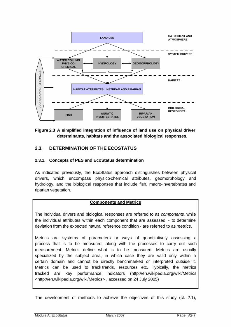
Figure 2.3 A simplified integration of influence of land use on physical driver determinants, habitats and the associated biological responses..........2-7
Figure 2.4 Reserve process indicating the interaction with EcoStatus and Components .........................................................................................2-13
Figure 3.1 Illustration of the Instream spreadsheet ................................................3-3 Figure 3.2 Levels of detail for EcoStatus determination for Reserve and RHP
purposes.................................................................................................3-6 Figure 3.3 EcoStatus Level 4 determination ...........................................................3-8 Figure 3.4 Illustration of the EcoStatus Level 4 model ...........................................3-9 Figure 3.5 EcoStatus Level 3 determination .........................................................3-10 Figure 3.6 Illustration of the summary of an EcoStatus assessment ...................3-16 Figure 4.1 Illustration of the summary of the alternative ECs.................................4-3 Figure 4.2 Illustration of summary of ecological consequences expressed in terms
of impact on EC......................................................................................4-3
Module A: EcoStatus March 2007 Page A1-1
1. ECOCLASSIFICATION
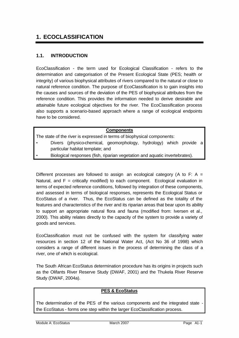
1.1. INTRODUCTION EcoClassification - the term used for Ecological Classification - refers to the determination and categorisation of the Present Ecological State (PES; health or integrity) of various biophysical attributes of rivers compared to the natural or close to natural reference condition. The purpose of EcoClassification is to gain insights into the causes and sources of the deviation of the PES of biophysical attributes from the reference condition. This provides the information needed to derive desirable and attainable future ecological objectives for the river. The EcoClassification process also supports a scenario-based approach where a range of ecological endpoints have to be considered.
Components The state of the river is expressed in terms of biophysical components: • Divers (physico-chemical, geomorphology, hydrology) which provide a
particular habitat template; and • Biological responses (fish, riparian vegetation and aquatic invertebrates).
Different processes are followed to assign an ecological category (A to F: A = Natural, and F = critically modified) to each component. Ecological evaluation in terms of expected reference conditions, followed by integration of these components, and assessed in terms of biological responses, represents the Ecological Status or EcoStatus of a river. Thus, the EcoStatus can be defined as the totality of the features and characteristics of the river and its riparian areas that bear upon its ability to support an appropriate natural flora and fauna (modified from: Iversen et al., 2000). This ability relates directly to the capacity of the system to provide a variety of goods and services. EcoClassification must not be confused with the system for classifying water resources in section 12 of the National Water Act, (Act No 36 of 1998) which considers a range of different issues in the process of determining the class of a river, one of which is ecological. The South African EcoStatus determination procedure has its origins in projects such as the Olifants River Reserve Study (DWAF, 2001) and the Thukela River Reserve Study (DWAF, 2004a).
PES & EcoStatus
The determination of the PES of the various components and the integrated state - the EcoStatus - forms one step within the larger EcoClassification process.
Module A: EcoStatus March 2007 Page A1-2
1.2. PROCEDURE The steps followed in EcoClassification are as follows: • Determination of the reference conditions for each component. • Determination of the PES for each component as well as for the EcoStatus. • Determination of the trend (i.e., movement towards or away from the
reference state) for each component as well as for the EcoStatus. • Determination of reasons for the PES and whether these are flow or non-flow
related. • Determination of the Ecological Importance and Sensitivity (EIS) for the biota
and habitat. • Proposing a realistic and attainable Recommended Ecological Category
(REC) for each component as well as for the EcoStatus by considering the PES and EIS.
• Determination of alternative Ecological Categories (ECs) for each component as well as for the EcoStatus.
These steps will be explained in more detail in the next sections. The flow diagram (Figure 1.1, adapted from DWAF, 2001) illustrates the process.

Module A: EcoStatus March 2007 Page A1-3
Figure 1.1 Flow diagram illustrating the information generated to determine the
range of ECs for which EWRs will be determined
Has the river changed from REFERENCE CONDITIONS due to
anthropogenic influences?
Ecological Category A PESHow much has the
condition/state changed?PES: EC A - F
Is the state still changing?TREND
What caused the changes?CAUSES
What are the origins of the causes?
SOURCES
Considering the EIS and the PES is it important / realistic to improve the
conditions?
IMPROVE MAINTAIN
Determine a realistically-attainable Recommended
Ecological Category
Determine the range of Ecological Categories to be
assessed
yes no
Determine EIS
Module A: EcoStatus March 2007 Page A1-4
1.2.1. Reference conditions The European Water Framework Directive (European Commission, 2000) defines a reference condition as the expected background condition with no or minimal anthropogenic stress and satisfying the following criteria: • It should reflect totally or nearly undisturbed conditions for hydro-
morphological elements, general physical and chemical elements, and biological quality elements.
• Concentrations of specific synthetic pollutants should be close to zero or below the limit of detection of the most advanced analytical techniques in general use.
More specifically, the reference condition describes the condition of the site, river reach or delineation prior to anthropogenic change and is formulated for each component considered in EcoStatus determination (fish, aquatic invertebrates, riparian vegetation, water quality, geomorphology and hydrology) following the process below: • Locate the least-impacted sites, either in the same or in ecologically
comparable river zones. • Use the results of historical ecological surveys before major human impacts.
If this is not possible, consider the use of survey information from ecologically comparable rivers. Use historical aerial photographs and land cover data to get an indication of the degree of catchment changes. The Internal Strategic Perspective (ISP) reports of the Department of Water Affairs and Forestry also provide relevant information.
• Use expert knowledge to derive an approximation of expected natural reference conditions.
Historical information and data, and/or data from reference sites (minimally impacted sites) are used to describe the reference conditions for the channel, hydrology, biota, and the water quality. Due to data limitations and/or the absence of any existing reference sites, the reference condition may not represent an actual natural river state, but rather the best estimate of a minimally impaired baseline state. If the river has not changed, then the PES can be described as being in a natural condition (Category A - see below). (DWAF, 2004a). Ideally, both qualitative and quantitative data are available either from historical origin or from other representative geographical regions. If only qualitative data is available, these can still be used, although this places limitations on the type of metrics that can be calculated and used in the assessment of the ecological quality (Nijboer et al. 2004).
Module A: EcoStatus March 2007 Page A1-5
Metric
Metrics are systems of parameters or ways of quantitative assessment of a process that is to be measured, along with the processes to carry out such measurement. Metrics define what is to be measured. Metrics are usually specialized by the subject area, in which case they are valid only within a certain domain and cannot be directly benchmarked or interpreted outside it. Metrics can be used to track trends and resources. Typically, the metrics tracked are key performance indicators. (http://en.wikipedia.org/wiki/Metrics <http://en.wikipedia.org/wiki/Metrics> , accessed on 24 July 2005). 1.2.2. Present Ecological State The PES of the river is expressed in terms of various components. That is, drivers (physico-chemical, geomorphology, hydrology) and biological responses (fish, riparian vegetation and aquatic invertebrates), as well as an integrated state, the EcoStatus.
The use of the term 'Ecological State' with reference to Drivers
Present Ecological States are determined for driver and response components. The term Ecological when describing the present state of the Drivers can strictly only be used in terms of the EcoClassification process. Therefore the present state categories of geomorphology and fish are both described using the term PES.
A rule-based procedure is followed to assign each component an Ecological Category (the PES) (A to F) using the following information: • Biophysical surveys conducted during the project. • Information and data from historical surveys, databases and reports. • Aerial photographs and videos. • Land-cover data. • Internal Strategic Perspective (ISP) reports of DWAF • Expert knowledge is regularly used to estimate the degree of change to a
particular component.
Ecological Category Definition
A comparison of the present biophysical conditions to the natural reference conditions. Description: The ecological category is used to define and type the ecological condition of a river in terms of the deviation of biophysical components from the natural reference condition. This is done through an assessment of the system drivers (physico-chemical, geomorphology, hydrology) that provide the habitat template for biota and the response of native biotic groups (fish, riparian vegetation and aquatic macro-invertebrates) to this template, as well as the response of native biota to introduced biota.
Module A: EcoStatus March 2007 Page A1-6
A A/B B B/C C C/D D D/E E E/F F
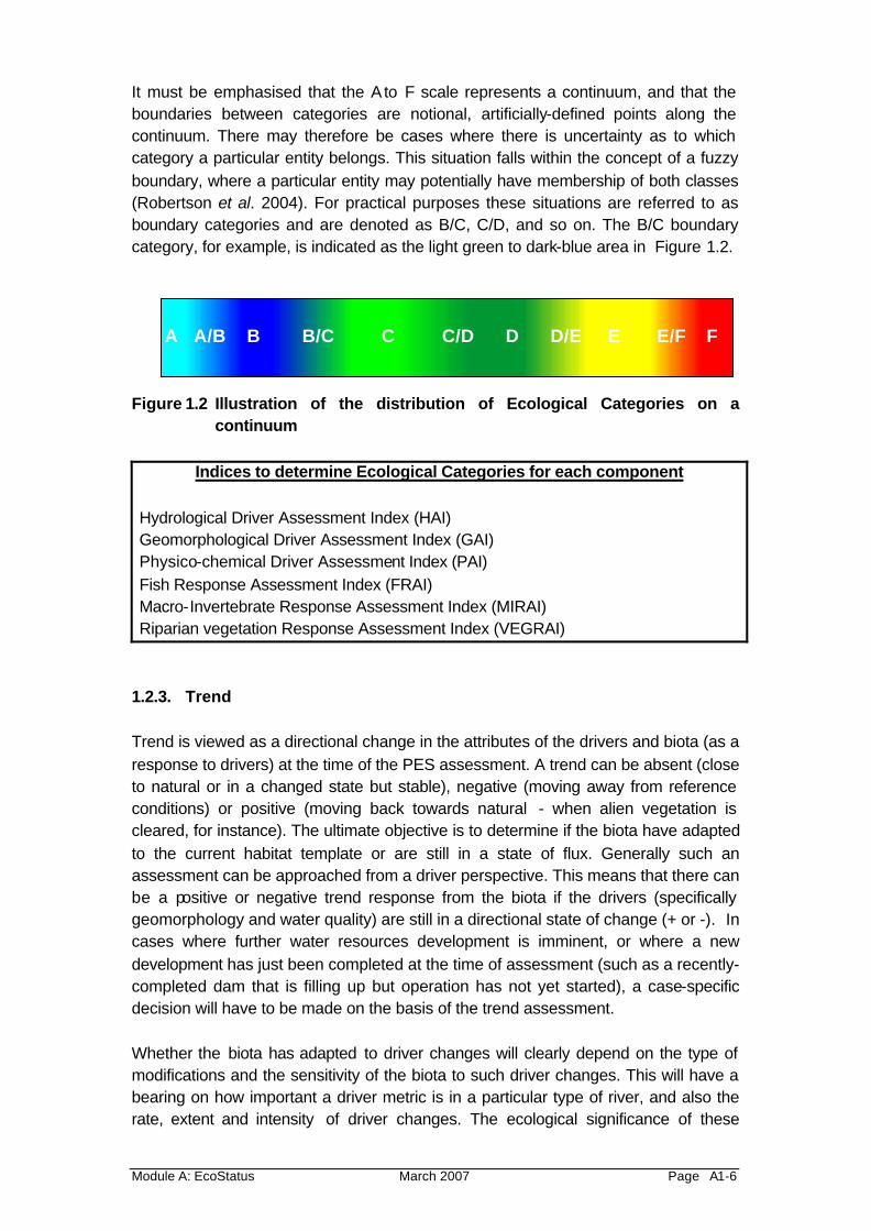
It must be emphasised that the A to F scale represents a continuum, and that the boundaries between categories are notional, artificially-defined points along the continuum. There may therefore be cases where there is uncertainty as to which category a particular entity belongs. This situation falls within the concept of a fuzzy boundary, where a particular entity may potentially have membership of both classes (Robertson et al. 2004). For practical purposes these situations are referred to as boundary categories and are denoted as B/C, C/D, and so on. The B/C boundary category, for example, is indicated as the light green to dark-blue area in Figure 1.2. Figure 1.2 Illustration of the distribution of Ecological Categories on a
continuum
Indices to determine Ecological Categories for each component Hydrological Driver Assessment Index (HAI) Geomorphological Driver Assessment Index (GAI) Physico-chemical Driver Assessment Index (PAI) Fish Response Assessment Index (FRAI) Macro-Invertebrate Response Assessment Index (MIRAI) Riparian vegetation Response Assessment Index (VEGRAI)
1.2.3. Trend Trend is viewed as a directional change in the attributes of the drivers and biota (as a response to drivers) at the time of the PES assessment. A trend can be absent (close to natural or in a changed state but stable), negative (moving away from reference conditions) or positive (moving back towards natural - when alien vegetation is cleared, for instance). The ultimate objective is to determine if the biota have adapted to the current habitat template or are still in a state of flux. Generally such an assessment can be approached from a driver perspective. This means that there can be a positive or negative trend response from the biota if the drivers (specifically geomorphology and water quality) are still in a directional state of change (+ or -). In cases where further water resources development is imminent, or where a new development has just been completed at the time of assessment (such as a recently-completed dam that is filling up but operation has not yet started), a case-specific decision will have to be made on the basis of the trend assessment. Whether the biota has adapted to driver changes will clearly depend on the type of modifications and the sensitivity of the biota to such driver changes. This will have a bearing on how important a driver metric is in a particular type of river, and also the rate, extent and intensity of driver changes. The ecological significance of these

Module A: EcoStatus March 2007 Page A1-7
driver changes will then be fundamental to the natural attributes of the biota in terms of resilience, adaptability and fragility. There will, then, be cases where the hydrology and water quality driver changes have occurred relatively recently but, at the time of the PES assessment, these drivers are stable (a recently-completed expansion of an irrigation area for instance, with associated increases in abstraction from the river and return flows into it). It is probable that the relative rates of change of these driver changes compared to geomorphology and biotic responses will be such that the geomorphology and biota is still in a state of flux. In these cases it will be necessary to make a qualitative interpretation of the rates of change by considering the extent to which the geomorphology and biota are expected to have responded to the driver changes in the short- to medium-term (five years) and long-term (20 years), and estimating the component categories that will prevail in the future. 1.2.4. PES cause-and-effect relationship
Causes
Disturbances and modifications that impact on the condition of a river can generally be viewed as stressors, and are considered as causes of ecological change.
Stressors occur at a particular intensity, duration and frequency that result in a change in the ecological conditions (US EPA 2000). The effect of the impact of stressors on the ecosystem are therefore, regarded as a response. In this context it is useful to consider causes, responses and the ultimate ecological effect in terms in ecological responses primarily related to flow modifications, and those primarily non-flow related, for instance: • A decrease in the abundance of a fish population or the species composition
of a fish assemblage may be interpreted as a response to a change in flow. However, where flow is unmodified, such population and assemblage changes may be attributable to primarily non-flow related causes such as sedimentation and physico-chemical changes.
• A decrease in riparian vegetation may be caused by catchment changes such as physical removal of vegetation by whatever means, with no link to modified flows. Obviously a decrease in riparian vegetation will be flow-related when flow is modified beyond the natural resilience of the riparian vegetation.
• Often however the causes are due to a combination of the impacts of flow and non-flow related sources. An example is sedimentation caused by land-use activities (non-flow related) that can be exacerbated by decreased flows due to irrigation (flow-related).
In the analysis of the cause-and-effect scenarios of the flow and non-flow related responses, it is often useful to define the source of a stressor. This is regarded as an entity or action that releases or imposes a stressor into the water body (US EPA 2000).
Module A: EcoStatus March 2007 Page A1-8
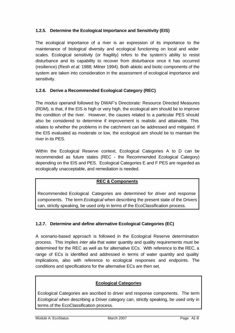
1.2.5. Determine the Ecological Importance and Sensitivity (EIS) The ecological importance of a river is an expression of its importance to the maintenance of biological diversity and ecological functioning on local and wider scales. Ecological sensitivity (or fragility) refers to the system’s ability to resist disturbance and its capability to recover from disturbance once it has occurred (resilience) (Resh et al. 1988; Milner 1994). Both abiotic and biotic components of the system are taken into consideration in the assessment of ecological importance and sensitivity. 1.2.6. Derive a Recommended Ecological Category (REC) The modus operandi followed by DWAF’s Directorate: Resource Directed Measures (RDM), is that, if the EIS is high or very high, the ecological aim should be to improve the condition of the river. However, the causes related to a particular PES should also be considered to determine if improvement is realistic and attainable. This relates to whether the problems in the catchment can be addressed and mitigated. If the EIS evaluated as moderate or low, the ecological aim should be to maintain the river in its PES. Within the Ecological Reserve context, Ecological Categories A to D can be recommended as future states (REC - the Recommended Ecological Category) depending on the EIS and PES. Ecological Categories E and F PES are regarded as ecologically unacceptable, and remediation is needed.
REC & Components
Recommended Ecological Categories are determined for driver and response components. The term Ecological when describing the present state of the Drivers can, strictly speaking, be used only in terms of the EcoClassification process.
1.2.7. Determine and define alternative Ecological Categories (EC) A scenario-based approach is followed in the Ecological Reserve determination process. This implies inter alia that water quantity and quality requirements must be determined for the REC as well as for alternative ECs. With reference to the REC, a range of ECs is identified and addressed in terms of water quantity and quality implications, also with reference to ecological responses and endpoints. The conditions and specifications for the alternative ECs are then set.
Ecological Categories
Ecological Categories are ascribed to driver and response components. The term Ecological when describing a Driver category can, strictly speaking, be used only in terms of the EcoClassification process.
Module A: EcoStatus March 2007 Page A1-9
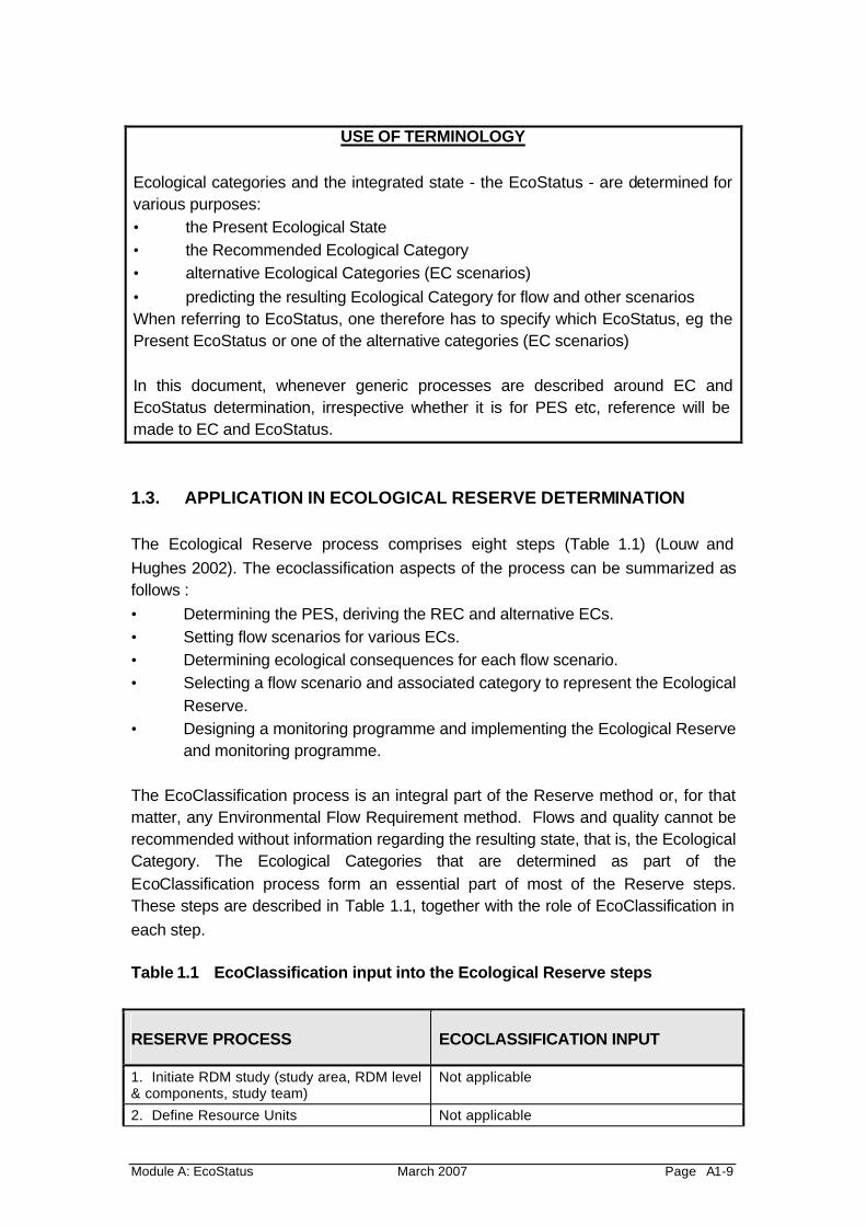
USE OF TERMINOLOGY
Ecological categories and the integrated state - the EcoStatus - are determined for various purposes: • the Present Ecological State • the Recommended Ecological Category • alternative Ecological Categories (EC scenarios) • predicting the resulting Ecological Category for flow and other scenarios When referring to EcoStatus, one therefore has to specify which EcoStatus, eg the Present EcoStatus or one of the alternative categories (EC scenarios) In this document, whenever generic processes are described around EC and EcoStatus determination, irrespective whether it is for PES etc, reference will be made to EC and EcoStatus. 1.3. APPLICATION IN ECOLOGICAL RESERVE DETERMINATION The Ecological Reserve process comprises eight steps (Table 1.1) (Louw and Hughes 2002). The ecoclassification aspects of the process can be summarized as follows : • Determining the PES, deriving the REC and alternative ECs. • Setting flow scenarios for various ECs. • Determining ecological consequences for each flow scenario. • Selecting a flow scenario and associated category to represent the Ecological
Reserve. • Designing a monitoring programme and implementing the Ecological Reserve
and monitoring programme. The EcoClassification process is an integral part of the Reserve method or, for that matter, any Environmental Flow Requirement method. Flows and quality cannot be recommended without information regarding the resulting state, that is, the Ecological Category. The Ecological Categories that are determined as part of the EcoClassification process form an essential part of most of the Reserve steps. These steps are described in Table 1.1, together with the role of EcoClassification in each step. Table 1.1 EcoClassification input into the Ecological Reserve steps
RESERVE PROCESS ECOCLASSIFICATION INPUT
1. Initiate RDM study (study area, RDM level & components, study team)
Not applicable
2. Define Resource Units Not applicable

Module A: EcoStatus March 2007 Page A1-10
RESERVE PROCESS ECOCLASSIFICATION INPUT
3. Define Ecological Categories and recommend one (REC)
Bulk of EcoClassification process: Determination of reference conditions, PES, EIS, REC and alternative ECs
4. Quantify Ecological Reserve Scenarios (flow scenarios)
Setting of flow scenarios for relevant ECs
5. Identify ecological consequences of flow scenarios (Ecological Reserve and operational flow scenarios)
Interpretation of consequences in terms of impact on ECs
6. DWAF Management Class decision making process.
Selection of a Management Class and associated EC
7. Reserve specification Determination of Resource Quality Objectives for specific ECs
8. Implementation design Design of a monitoring programme to monitor achievement of the EC associated with the Management Class
IMPLEMENT AND MONITOR Evaluation in terms of EC.
1.4. APPLICATION WITHIN MONITORING Beechie et al. (2003) point out that there are five types of uncertainty in predictions of habitat capacity : • Predictive uncertainty, which refers to the difference between the modelled
response and the “true” response. • Parameter uncertainty, which refers to the difference between the “true”
parameter (such as an average or a regression coefficient) and the parameter as estimated from the data.
• Model uncertainty, which refers to the difference between the natural system and the mathematical equation used to describe it.
• Measurement uncertainty, which refers to the difference between the “true” value and the recorded value.
• Natural stochastic variation, which refers to the inherent random variability. These uncertainties are also relevant to the Ecological Reserve determination process, where qualitative data, expert knowledge and judgment often have to be used due to a lack of empirical information on ecological requirements in particular. The time frame to obtain such information is usually very limited and the only practical way to deal with this uncertainty is through a well-designed monitoring and assessment process. In the Ecological Reserve context the purpose of monitoring is to determine if the required EC is attained. If this is not the case, monitoring data is used in an adaptive management fashion (Rogers and Bestbier 1997) to reconsider, re-calibrate and possibly re-construct the specifications that have been set for the biophysical components that relate to a particular desired management goal or EC. The procedure of adaptive resource management involves following the EcoClassification process to assess biophysical conditions and responses critically, to determine the
Module A: EcoStatus March 2007 Page A1-11
current EC, resulting from the implementation of the Ecological Reserve specifications, and to compare it with REC. Biological monitoring for the River Health Programme (RHP), also uses EcoClassification to assess data in terms of the severity of changes. However, the RHP focuses primarily on biological responses as an indicator of ecosystem health, with only a vague cause-and-effect relationship between the drivers and the biological responses. Within the concept of adaptive resource management, if the biological integrity indicates the possibility of generally unacceptable conditions (such as indicated by thresholds of probable concern being exceeded (Rogers and Bestbier 1997), more detailed monitoring is indicated to determine the cause and the severity of the problem and to instigate management intervention to rectify the problem. The RHP focuses on the reference conditions and PES steps of the EcoClassification process. ___________________________________________________________________
Module A: EcoStatus March 2007 Page A2-1
2. ECOSTATUS INTRODUCTION
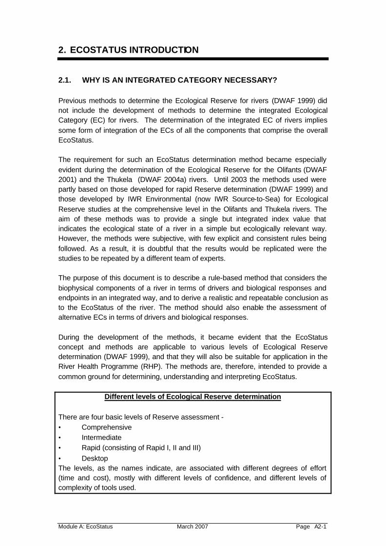
2.1. WHY IS AN INTEGRATED CATEGORY NECESSARY? Previous methods to determine the Ecological Reserve for rivers (DWAF 1999) did not include the development of methods to determine the integrated Ecological Category (EC) for rivers. The determination of the integrated EC of rivers implies some form of integration of the ECs of all the components that comprise the overall EcoStatus. The requirement for such an EcoStatus determination method became especially evident during the determination of the Ecological Reserve for the Olifants (DWAF 2001) and the Thukela (DWAF 2004a) rivers. Until 2003 the methods used were partly based on those developed for rapid Reserve determination (DWAF 1999) and those developed by IWR Environmental (now IWR Source-to-Sea) for Ecological Reserve studies at the comprehensive level in the Olifants and Thukela rivers. The aim of these methods was to provide a single but integrated index value that indicates the ecological state of a river in a simple but ecologically relevant way. However, the methods were subjective, with few explicit and consistent rules being followed. As a result, it is doubtful that the results would be replicated were the studies to be repeated by a different team of experts. The purpose of this document is to describe a rule-based method that considers the biophysical components of a river in terms of drivers and biological responses and endpoints in an integrated way, and to derive a realistic and repeatable conclusion as to the EcoStatus of the river. The method should also enable the assessment of alternative ECs in terms of drivers and biological responses. During the development of the methods, it became evident that the EcoStatus concept and methods are applicable to various levels of Ecological Reserve determination (DWAF 1999), and that they will also be suitable for application in the River Health Programme (RHP). The methods are, therefore, intended to provide a common ground for determining, understanding and interpreting EcoStatus.
Different levels of Ecological Reserve determination
There are four basic levels of Reserve assessment - • Comprehensive • Intermediate • Rapid (consisting of Rapid I, II and III) • Desktop The levels, as the names indicate, are associated with different degrees of effort (time and cost), mostly with different levels of confidence, and different levels of complexity of tools used.
Module A: EcoStatus March 2007 Page A2-2
Why the same EcoStatus approach for Ecological Reserve and River Health Programme?
The determination of the Present Ecological State is common to both the Ecological Reserve and the RHP. The Ecological Reserve and RHP can support each other. Descriptions (by means of Ecological Category) therefore must have the same meaning when they are used in either the Ecological Reserve or the RHP. This implies that the same tools and indices should be used.
2.2. ECOSTATUS: SCIENTIFIC RATIONALE The EcoStatus approach is centred around a number of concepts and principles. 2.2.1. Ecosystem integrity / health concepts Conceptual attributes that comprise ecosystem health (i.e. if this is present the system will be healthy) are summarized by Costanza (1992): • Homeostasis (tendency of biological systems to maintain a state of
equilibrium) • Absence of disease • Diversity or complexity • Stability or resilience • Vigour or scope for growth • Balance between system components Following from these concepts of ecosystem health, the sequence for ecosystem health assessment can be viewed as embracing the following steps (Shaeffer et al 1988): • Identify symptoms of ill health • Identify and measure signs of ill health • Make provisional diagnosis of the causes of ill health • Conduct tests to verify the diagnosis • Make a prognosis • Prescribe treatment 2.2.2. EcoStatus of rivers The following description of the EcoStatus of rivers was found to be the most appropriate to the EcoClassification approach followed in South Africa.
EcoStatus Definition
“The totality of the features and characteristics of the river and its riparian areas that bear upon its ability to support an appropriate natural flora and fauna and its capacity to provide a variety of goods and services" (Iversen et al 2000).
Module A: EcoStatus March 2007 Page A2-3
A river will have a natural/close-to-natural EcoStatus when the components below are close to natural (Iversen et al 2000). a) Hydro-morphology (Geomorphology and Hydrology) The quantity and dynamics of flow reflect almost undisturbed conditions. The continuity of the river allows undisturbed migration of aquatic organisms and sediment transport. Channel patterns, width and depth variations, flow velocities, substrate conditions and both the structure and condition of the riparian zones correspond to almost-undisturbed conditions. b) Water quality • The values of the physico-chemical elements correspond to almost-
undisturbed conditions. • Nutrient concentrations remain within the range normally associated with
undisturbed conditions. • Levels of salinity, pH, oxygen balance, acid neutralising capacity and
temperature remain within the range normally associated with almost undisturbed conditions.
• Synthetic and non-synthetic pollutants are close to zero. c) Biology The taxonomic composition and abundance of the riparian vegetation, phytoplankton, macrophytes, invertebrates and fish correspond very closely to the undisturbed conditions. 2.2.3. Indicators of ecosystem integrity / health Environmental indicators of ecosystem health can be categorized as follows (Yoder et al. 2000; Novotny et al. 2005): a) Stressors These refer to large-scale influences that generally originate from anthropogenic activities, and include point and non-point loadings (including atmospheric deposition), land use influences and changes, and stream modification. b) Exposure indicators These include chemical parameters, whole-effluent toxicity, tissue residues, sediment contamination, habitat degradation and other changes that result in a risk to the biota.
c) Response indicators or biotic assessment endpoints These are the direct measures of ecological integrity or ecological status. Biota is the highest level of effects of propagation of stresses throughout the ecosystem. It is desirable that endpoint indicators express three dimensions of integrity. • Physical integrity implies habitat conditions of the water body that would
sustain a balanced biological community.
Module A: EcoStatus March 2007 Page A2-4
• Physico-chemical integrity (referring both to chemical and physical properties of the water) refers to water and sediments that are not injurious to the aquatic biota.
• A composition of aquatic biota that is balanced, and resembles or approaches that of unaffected similar aquatic systems in the same EcoRegion without invasive species, represents biological integrity.
It is preferable that all three dimensions of endpoint assessment are conducted concurrently ( Novotny et al. 2005). 2.2.4. A layered approach to aquatic ecosystem integrity assessment
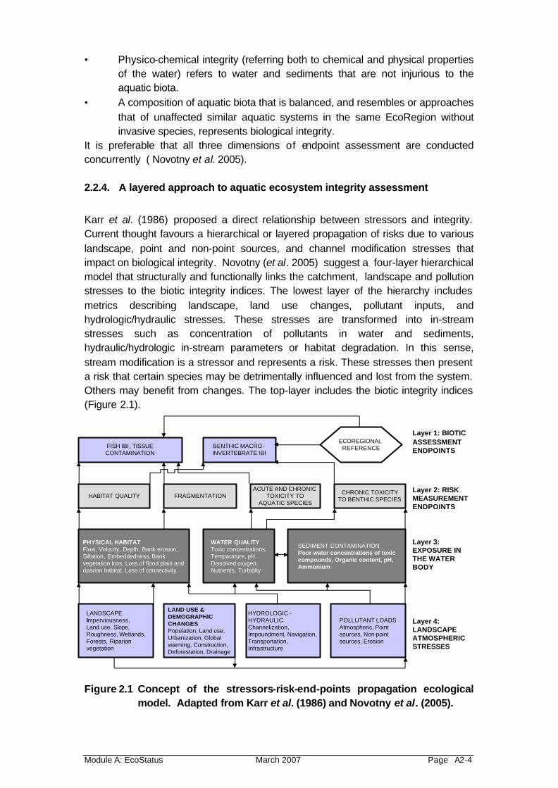
Karr et al. (1986) proposed a direct relationship between stressors and integrity. Current thought favours a hierarchical or layered propagation of risks due to various landscape, point and non-point sources, and channel modification stresses that impact on biological integrity. Novotny (et al. 2005) suggest a four-layer hierarchical model that structurally and functionally links the catchment, landscape and pollution stresses to the biotic integrity indices. The lowest layer of the hierarchy includes metrics describing landscape, land use changes, pollutant inputs, and hydrologic/hydraulic stresses. These stresses are transformed into in-stream stresses such as concentration of pollutants in water and sediments, hydraulic/hydrologic in-stream parameters or habitat degradation. In this sense, stream modification is a stressor and represents a risk. These stresses then present a risk that certain species may be detrimentally influenced and lost from the system. Others may benefit from changes. The top-layer includes the biotic integrity indices (Figure 2.1).
Figure 2.1 Concept of the stressors-risk-end-points propagation ecological
model. Adapted from Karr et al. (1986) and Novotny et al. (2005).
LANDSCAPEImperviousness,Land use, Slope, Roughness, Wetlands, Forests, Riparian vegetation
LAND USE & DEMOGRAPHIC CHANGESPopulation, Land use, Urbanization, Global warming, Construction, Deforestation, Drainage
HYDROLOGIC -HYDRAULICChannelization, Impoundment, Navigation, Transportation, Infrastructure
POLLUTANT LOADSAtmospheric, Point sources, Non-point sources, Erosion
PHYSICAL HABITATFlow, Velocity, Depth, Bank erosion, Siltation, Embeddedness, Bank vegetation loss, Loss of flood plain and riparian habitat, Loss of connectivity
WATER QUALITYToxic concentrations, Temparature, pH, Dissolved oxygen, Nutrients, Turbidity
SEDIMENT CONTAMINATIONPoor water concentrations of toxic compounds, Organic content, pH, Ammonium
HABITAT QUALITY FRAGMENTATIONACUTE AND CHRONIC
TOXICITY TO AQUATIC SPECIES
CHRONIC TOXICITY TO BENTHIC SPECIES
FISH IBI , TISSUE CONTAMINATION
BENTHIC MACRO-INVERTEBRATE IBI
ECOREGIONALREFERENCE
Layer 1: BIOTIC ASSESSMENT ENDPOINTS
Layer 2: RISK MEASUREMENT ENDPOINTS
Layer 3: EXPOSURE IN THE WATER BODY
Layer 4: LANDSCAPE ATMOSPHERIC STRESSES
Module A: EcoStatus March 2007 Page A2-5
2.2.5. Layer 1: Dependent variables; biotic assessment endpoints Indices based on fish and macro-invertebrate assemblages are most often used as measures of species diversity, composition and ecological health. The outcome of such an index evaluation is a single number scoring summary but, each index also has a multimetric dimension. This means that some metrics are more affected by habitat and physical features of the channel and its riparian zone, some by flow characteristics, and some - such as deformities, erosion, lesions and tumours and species diversity - by pollutants (such as siltation, nutrients, toxics) and embeddedness. 2.2.6. Layer 2: Risks - measurement endpoints Risks are viewed as a probabilistic potential for loss of species or genera from a system. Significant risks are associated with pollutants stored in sediments and habitat degradation. Four biological categories are affected by chemical or channel disturbance specific risks - survival, growth, reproduction and fragmentation. However, in some instances invasion by introduced (alien) species can pose a significant risk and influence the ecological risk. The risks include: • Pollutant (physico-chemical) risks (acute and chronic) in the water column.
Key metrics are toxic pollutants, dissolved oxygen, turbidity, temperature and pH.
• Pollutant risk (mostly chronic) in the sediment. Key metrics include toxic pollutants, ammonium, dissolved oxygen in the interstitial layer, organic and clay content.
• Habitat degradation risk. Key metrics include texture of the sediment, clay and organic contents, embeddedness, pools and riffle structure, bank stability, riparian zone quality, canalisation and other stream modifications.
• Fragmentation risk. This risk can result from any factor (biotic or abiotic) that causes decrease in the ability of species to migrate among subpopulations or between portions of their habitat necessary for different life-cycle stages.
Key metrics include: • Longitudinal – presence of dams, weirs and impassable culverts. • Lateral – Lining, embankments, loss of riparian habitat, reduction or
elimination of refugia. • Vertical – lack of the stream-groundwater interchange, thermal stratification /
heated discharges, bottom lined channel. 2.2.7. Layer 3: Instream exposure stressors Generally, these express the level of chemical and bacteriological contamination of water and sediment, channel and stream bank stability, flow and temperature variability and riparian zone effects. Transfer functions link this layer with the landscape inputs. Such functions include pollutant dilution, dissolved oxygen (steady state and variability due to eutrophication), nutrient models, sedimentation, flow and

Module A: EcoStatus March 2007 Page A2-6
temperature. Parameters affecting habitat suitability risk are usually included in the list of metrics defining habitat indices. Some of these are related to hydrological parameters such as high-flow / low-flow frequencies, velocity, frequency of bankfull flows and channel morphology (slope, channel dimensions, pool and riffle sequence, sinuosity). 2.2.8. Layer 4: Catchment stresses Four groups of these stresses can be recognized: • Morphological and riparian factors and stresses. • Land use change stresses. • Diffuse pollutant sources (land and atmosphere) and point source discharges. • Hydrologic changes. 2.2.9. Current approach Beechie and Boulton (1999) propose an approach similar to that of Novotny et al. (2005), where the biological fitness and survival (biological responses) in an aquatic ecosystem are determined through layers or linkages of controls or drivers to processes and to habitat effects (Figure 2.2). The essence of this interpretation is that the direct assessment of the biological response (e.g., using a biological indicator) identifies where ecosystem functions have been impaired, and may suggest causes of impairment (Beechie et al. 2003). This provides the general framework that was used to develop conceptual approaches and assessment models within which the current project was carried out (Figure 2.2).
Figure 2.2 Schematic diagram of relationships between controls on catchment
processes, effects on habitat conditions, and aquatic biota survival and fitness. Black boxes indicate controls not affected by land use (adapted from Beechie and Bolton 1999).
SEDIMENT SUPPLY
HYDROLOGIC REGIME
ORGANIC MATTER INPUTS
NUTRIENT / CHEMICAL
INPUTS
LIGHT / HEAT INPUTS
PHYSICAL HABITAT CHARACTERISTICS
WATER QUALITY AND PRIMARY PRODUCTIVITY
BIOLOGICAL FITNESS AND SURVIVAL
GEOLOGYVEGETATION CLIMATE
GROSS REACH MORPHOLOGYLAND USES
CONTROLS / DRIVERS
PROCESSES
HABITAT EFFECTS
BIOLOGICAL RESPONSES
Module A: EcoStatus March 2007 Page A2-7
Figure 2.3 A simplified integration of influence of land use on physical driver
determinants, habitats and the associated biological responses. 2.3. DETERMINATION OF THE ECOSTATUS 2.3.1. Concepts of PES and EcoStatus determination As indicated previously, the EcoStatus approach distinguishes between physical drivers, which encompass physico-chemical attributes, geomorphology and hydrology, and the biological responses that include fish, macro-invertebrates and riparian vegetation.
Components and Metrics
The individual drivers and biological responses are referred to as components, while the individual attributes within each component that are assessed - to determine deviation from the expected natural reference condition - are referred to as metrics. Metrics are systems of parameters or ways of quantitatively assessing a process that is to be measured, along with the processes to carry out such measurement. Metrics define what is to be measured. Metrics are usually specialized by the subject area, in which case they are valid only within a certain domain and cannot be directly benchmarked or interpreted outside it. Metrics can be used to track trends, resources etc. Typically, the metrics tracked are key performance indicators (http://en.wikipedia.org/wiki/Metrics <http://en.wikipedia.org/wiki/Metrics> , accessed on 24 July 2005) The development of methods to achieve the objectives of this study (cf. 2.1),
FISH AQUATIC INVERTEBRATES
RIPARIAN VEGETATION
FISH AQUATIC INVERTEBRATES
RIPARIAN VEGETATION
HABITAT ATTRIBUTES: INSTREAM AND RIPARIAN
WATER COLUMN: PHYSICO-CHEMICAL
HYDROLOGY GEOMORPHOLOGYWATER COLUMN:
PHYSICO-CHEMICAL
HYDROLOGY GEOMORPHOLOGY
LAND USECATCHMENT AND ATMOSPHERE
SYSTEM DRIVERS
HABITAT
BIOLOGICAL RESPONSES
EC
OR
EG
ION
AL
RE
FE
RN
CE
S
Module A: EcoStatus March 2007 Page A2-8
focussed on a two-step process (Joubert 2004): • Devising consistent indices for the assessment of the EC of individual
biophysical components. • Devising a consistent process whereby the EC of individual components can
be integrated at various levels to derive the EcoStatus of the river. The principle followed here is that the biological responses integrate the effect of the modification of the drivers and that this results in an ecological endpoint (cf. 2.2.4). This endpoint can be quantifiable, or it may be described in a predominantly qualitative fashion, and is presented in the form of a multimetric index. This approach means that: • The driver components are assessed separately (that is, an EC for each
driver) and not integrated at the driver level. However, the individual metrics of all the driver components are assessed in a combined fashion that allows some comparison between metrics of all drivers. This facilitates deriving the cause-and-effect relationships that are required in the interpretation and assessment of particular biological responses.
• The biological responses are assessed separately, but the resulting fish and macro-invertebrate ECs are integrated to provide an indication of the instream EC. The integration of the riparian vegetation EC and the instream EC provides the EcoStatus.
Indices and models
Indices are determined for all the Driver and Response components using a rule-based modelling approach. The names of the models refer to indices, eg Hydrology Driver Assessment Index and Fish Response Assessment Index. 2.3.2. Rating, ranking and weighting, and integrating The basis of the assessment of the importance of the metrics of biophysical components in determining the EC and EcoStatus is a Multi Criteria Decision Analysis approach (MCDA). The MCDA process allows the development of consistent rating systems or indices for the categorisation of ecosystem components and aggregates these mathematically in a theoretically justifiable way. In the current approach, the MCDA input was limited to the elicitation of weights for the aggregation of the subindices and indices (Joubert 2004). 2.3.3. Rating (Scoring) A six-point rating system is followed, where metrics of the drivers and biological responses are scored in terms of the degree to which they have changed compared to the natural or close-to-natural reference (if necessary, half points such as 1.5 and so on can also be used) -
0 = No discernable change from reference/close to reference 1 = Small modification from reference 2 = Moderate modification from reference
Module A: EcoStatus March 2007 Page A2-9
3 = Large modification from reference 4 = Serious modification from reference 5 = Extreme modification from reference
These qualitative ratings are expert knowledge-based, and are assessed by the relevant expert in a particular speciality. It is preferable that the relative difference between for example, 0 – 1 be the same as between 3 – 4 (Joubert 2004). However, this is difficult to control and is currently exclusively based on expert knowledge. In the case of fish, a modified approach is followed where changes in some metrics are interpreted in terms of an increase or decrease. This will be discussed further in the Module D.
Rating
The rating requires different metrics to be scored according to the relative degree of change from reference conditions.
2.3.4. Ranking and weighting The principle of following a ranking-weighting approach is that not all driver or biological response metrics have the same relative ecological significance in all types of rivers. That is, a particular metric may be seriously modified but it may be of relatively low significance in terms of the functioning and integrity of the river. In another river (or a different section of the same river) in a different ecoregional context (Kleynhans et. al 2004), this metric may, however, be of very high ecological importance. Thus, the ranking-weighting process is done separately from the rating and should not be influenced by it. Ranking is done as follows - The metric of the component (driver or biological response) that is considered to be most important in influencing the EC of the component if it changed is ranked as 1. This can be formulated as:
Considering the range from 5 to 0 of each of these metrics, which one would most affect the component (driver or biological response) if it changed from 0 to 5? (irrespective of the rating actually applied) (Joubert 2004). The next most important metric is ranked as 2, then 3, and so on.
Another way of posing this question is: Considering the range from 0 to 5, if a particular component is considered, which metric would contribute most to improving (or decreasing) the PES. The next most important metric is ranked as 2, then 3, and so on.
In terms of geomorphology, the Index of Habitat integrity, fish, invertebrates and riparian vegetation, these components are divided into metric-groups. The questions posed above then apply to each of the metrics in a metric group. In assessing the importance of a metric group in terms of its contribution to the EC of the component,
Module A: EcoStatus March 2007 Page A2-10
a similar ranking procedure is followed - the metric group considered to be the most important in determining the EC of the component is ranked 1, and so on. The ranking procedure is essentially used to guide the weighting process and, except for a check-up function, plays no further role in the calculation of weights and weighted scores. Where it is not possible to distinguish between the relative importance of metrics (or metric-groups), a rank of 1 should be awarded to all metrics. Weighting is done as follows: The metric (or metric-group, cf. above) with a rank of 1 is awarded a weight of 100%. The weight of the metric with a rank of 2 is considered relative to its importance when compared to the metric with a rank = 1, and this can be any percentage lower than 100%. Usually expert knowledge limits the resolution to 10% and sometimes 5%. Where all metrics (or metric-groups) are ranked as 1, they will all receive a weight of 100%.
Weighting
The weighting is required to provide an indication of the importance of the degree that the metrics have changed (that is, the rating) 2.3.5. Calculation of weighted scores The percentage weight of each metric (or metric -group where applicable) is expressed as a proportion of the total of the percentage weights. This value is multiplied by: • the rating, • the total number of metrics considered and • the maximum possible score (5) to provide a weighted score for a metric. Where the weight of all metrics (or metric-groups) is 100%, the original rating will obviously be applicable. 2.3.6. Calculation of ECs for components The calculation of the Ecological Categories of drivers and biological responses is done by totalling the weighted scores and expressing this as a percentage of the maximum. This value indicates the percentage change away from the expected reference and must be subtracted from 100 to arrive at the percentage value that represents the EC. This value is used to place the EC of the component in a particular category that ranges from A to F (Table 2.10). Where metric-groups are used, the same approach is followed for each group.

Module A: EcoStatus March 2007 Page A2-11
However, with metric-groups, the calculation of the overall EC for a component follows a slightly different approach. In this case the EC value for each metric group is multiplied by the weight of the metric group to provide a weighted score for the group as a percentage, which is then related to an EC ( Table 2.1). Table 2.1 Generic ecological categories for EcoStatus components (modified
from Kleynhans 1996 & Kleynhans 1999).
ECOLOGICAL CATEGORY
DESCRIPTION SCORE (% OF TOTAL)
A Unmodified, natural. 90-100
B Largely natural with few modifications. A small change in natural habitats and biota may have taken place but the ecosystem functions are essentially unchanged.
80-89
C Moderately modified. Loss and change of natural habitat and biota have occurred, but the basic ecosystem functions are still predominantly unchanged.
60-79
D Largely modified. A large loss of natural habitat, biota and basic ecosystem functions has occurred.
40-59
E Seriously modified. The loss of natural habitat, biota and basic ecosystem functions is extensive.
20-39
F Critically / Extremely modified. Modifications have reached a critical level and the system has been modified completely with an almost complete loss of natural habitat and biota. In the worst instances the basic ecosystem functions have been destroyed and the changes are irreversible.
0-19
2.3.7. Methods for EcoStatus integration After the Ecological Categories of the driver and ecological response components have been determined (cf.2.3.2), there remains the issue of how to integrate these to provide an indication of the EcoStatus. Deriving the EcoStatus from the Ecological Categories of components is based on the following principles: • The Ecological Categories of the physical drivers (hydrology, geomorphology
and physico-chemical integrity) are not integrated to provide a driver status. • Information on the driver metrics: how different they are from the reference is
considered when assessing the biological responses. This is an expert knowledge approach and the attributes and environmental requirements of the biota should be considered when doing this.
• The biological responses are considered to provide the best indication of the EcoStatus of the river because they integrate the effect of the driver components (cf.Figure 2.2; Beechie et al. 2003)
The steps in deriving the EcoStatus are: • Criteria are considered that provide an indication of the relative indicator
value of the two instream biological groups, fish and invertebrates. These criteria are used to weight the relative importance of these two groups as indicators of instream health. The Ecological Categories of the two biological groups are proportioned according to these weights and combined to provide
Module A: EcoStatus March 2007 Page A2-12
the instream Ecological Category. • The Vegetation Response Assessment Index is used to obtain the riparian
vegetation Ecological Category. • The riparian vegetation Ecological Category and the instream Ecological
Category are integrated based on a proportioning of weights according to the availability of high confidence information. This provides the EcoStatus of the river.
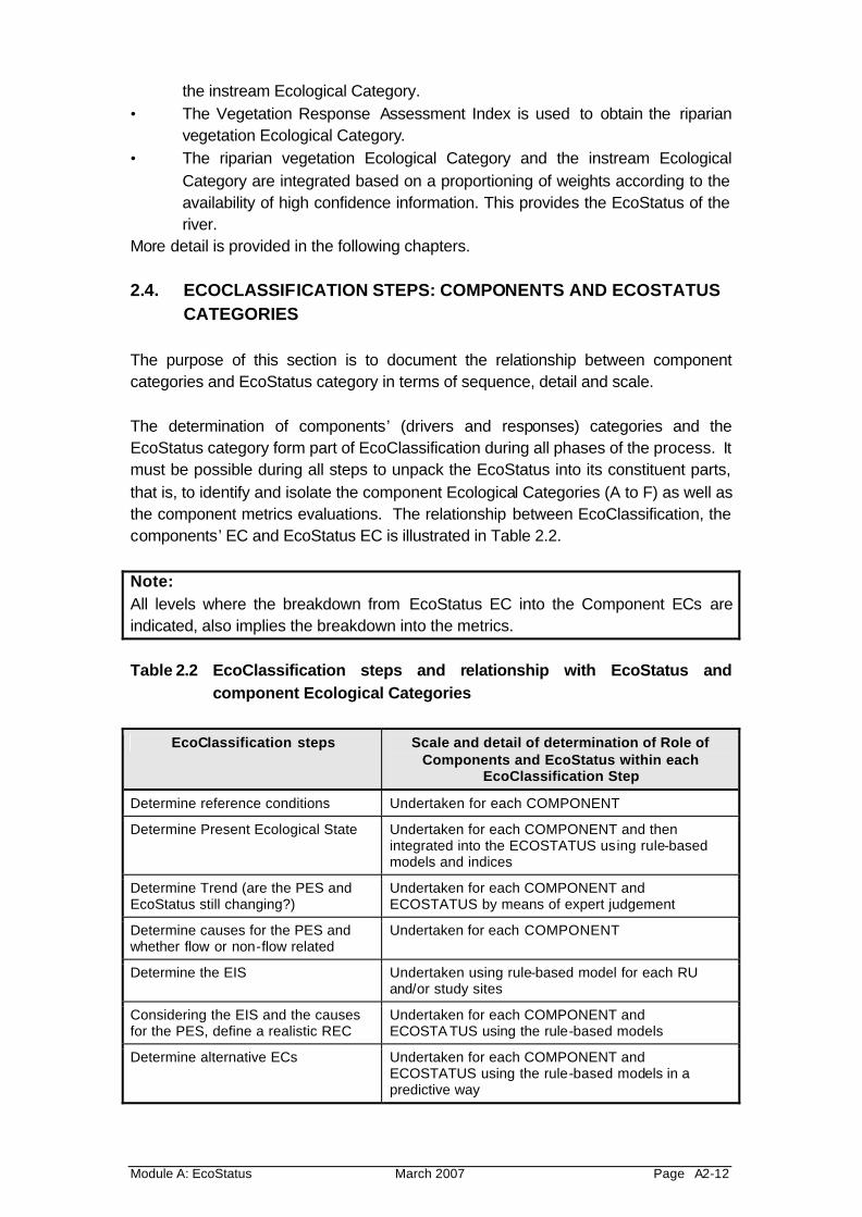
More detail is provided in the following chapters. 2.4. ECOCLASSIFICATION STEPS: COMPONENTS AND ECOSTATUS
CATEGORIES The purpose of this section is to document the relationship between component categories and EcoStatus category in terms of sequence, detail and scale. The determination of components’ (drivers and responses) categories and the EcoStatus category form part of EcoClassification during all phases of the process. It must be possible during all steps to unpack the EcoStatus into its constituent parts, that is, to identify and isolate the component Ecological Categories (A to F) as well as the component metrics evaluations. The relationship between EcoClassification, the components’ EC and EcoStatus EC is illustrated in Table 2.2. Note: All levels where the breakdown from EcoStatus EC into the Component ECs are indicated, also implies the breakdown into the metrics. Table 2.2 EcoClassification steps and relationship with EcoStatus and
component Ecological Categories
EcoClassification steps Scale and detail of determination of Role of Components and EcoStatus within each
EcoClassification Step
Determine reference conditions Undertaken for each COMPONENT
Determine Present Ecological State Undertaken for each COMPONENT and then integrated into the ECOSTATUS using rule-based models and indices
Determine Trend (are the PES and EcoStatus still changing?)
Undertaken for each COMPONENT and ECOSTATUS by means of expert judgement
Determine causes for the PES and whether flow or non-flow related
Undertaken for each COMPONENT
Determine the EIS Undertaken using rule-based model for each RU and/or study sites
Considering the EIS and the causes for the PES, define a realistic REC
Undertaken for each COMPONENT and ECOSTA TUS using the rule-based models
Determine alternative ECs Undertaken for each COMPONENT and ECOSTATUS using the rule-based models in a predictive way
Module A: EcoStatus March 2007 Page A2-13
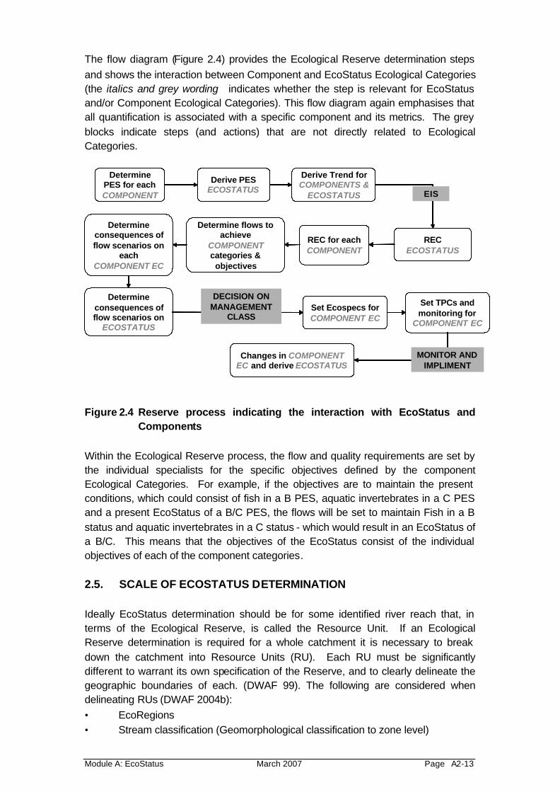
The flow diagram (Figure 2.4) provides the Ecological Reserve determination steps and shows the interaction between Component and EcoStatus Ecological Categories (the italics and grey wording indicates whether the step is relevant for EcoStatus and/or Component Ecological Categories). This flow diagram again emphasises that all quantification is associated with a specific component and its metrics. The grey blocks indicate steps (and actions) that are not directly related to Ecological Categories.
Figure 2.4 Reserve process indicating the interaction with EcoStatus and
Components Within the Ecological Reserve process, the flow and quality requirements are set by the individual specialists for the specific objectives defined by the component Ecological Categories. For example, if the objectives are to maintain the present conditions, which could consist of fish in a B PES, aquatic invertebrates in a C PES and a present EcoStatus of a B/C PES, the flows will be set to maintain Fish in a B status and aquatic invertebrates in a C status - which would result in an EcoStatus of a B/C. This means that the objectives of the EcoStatus consist of the individual objectives of each of the component categories. 2.5. SCALE OF ECOSTATUS DETERMINATION Ideally EcoStatus determination should be for some identified river reach that, in terms of the Ecological Reserve, is called the Resource Unit. If an Ecological Reserve determination is required for a whole catchment it is necessary to break down the catchment into Resource Units (RU). Each RU must be significantly different to warrant its own specification of the Reserve, and to clearly delineate the geographic boundaries of each. (DWAF 99). The following are considered when delineating RUs (DWAF 2004b): • EcoRegions • Stream classification (Geomorphological classification to zone level)
Determine PES for each COMPONENT
Derive PES ECOSTATUS
Derive Trend for COMPONENTS &
ECOSTATUS
REC ECOSTATUS
REC for each COMPONENT
Determine consequences of flow scenarios on
each COMPONENT EC
Set Ecospecs for COMPONENT EC
Set TPCs and monitoring for
COMPONENT EC
Changes in COMPONENT EC and derive ECOSTATUS
DECISION ON MANAGEMENT
CLASS
EIS
Determine consequences of flow scenarios on
ECOSTATUS
MONITOR AND IMPLIMENT
Determine flows to achieve
COMPONENTcategories &
objectives

Module A: EcoStatus March 2007 Page A2-14
• Habitat Integrity • Water quality delineation into units • Groundwater units (if applicable or available) • Operation of the system During a Comprehensive assessment of the Ecological Reserve, sufficient information should be available to apply the EcoClassification for the RU as a whole. This is, for example, aided by an aerial video that is available for the whole river, as well as a habitat integrity assessment for the river. Specific study sites (called IFR or EWR sites) are also selected within each RU, where detailed sampling and surveying are undertaken. Within the Intermediate assessment, less information will be available, and knowledge of the river reach is obtained from ground surveys and local knowledge rather than an aerial survey and video. The process followed is, however, the same as for the Comprehensive assessment. During the Rapid III assessment, RUs are not necessarily identified due to the time constraints associated with a rapid assessment. Available EcoRegion information is used to provide some perspective of RUs and to put the results into context. In essence, the EcoRegions and obvious operational information (if relevant) will inform the RU identification. The EcoStatus information is however targeted more towards the site than the RU due usually to lack of available information about the larger RU. Within the RHP the scale and delineation of the resource for EcoStatus assessment vary widely. EcoRegions form the basis of the assessment and, within these, catchments with similar kinds of impacts are usually combined, while DWAF management units are also taken into consideration. The combination of these is termed assessment units. ___________________________________________________________________

Module A: EcoStatus March 2007 Page A3-1
3. ECOSTATUS DETERMINATION
3.1. ASSESSMENT OF DRIVERS As pointed out (cf.2.3.7), metrics of each driver component are integrated to provide an Ecological Category (EC) for each component. However, the three drivers are not integrated to provide a driver EC. The information required from the drivers refers to the information contained in individual metrics, and which can be used to interpret habitat required by the biota. This information can then be used to determine and explain biological responses. 3.2. USE AND INTERPRETATION OF DRIVER METRICS FOR
INSTREAM BIOLOGICAL RESPONSES The basis of this approach is the general biological response that would be expected from the instream biota and riparian vegetation given a particular combination of driver conditions. The following are the essential aspects of this approach - • As pointed out (cf.2.3.7), metrics of each driver component are integrated to
provide an EC for each component. This provides an overall indication of the habitat template to which the biota would respond.
• However, for the interpretation and assessment of biological responses, individual driver metrics should also be looked at and interpreted. Metrics that indicate, for example, changes in the flow conditions (such as an increase in the frequency of low flow conditions), provide important information as to the way instream biota would respond.
• The reference condition, temporal and spatial characteristics of the habitat are key considerations for the interpretation of habitat and biological responses. Biological responses are determined and explained qualitatively.
3.3. DETERMINATION OF INSTREAM RESPONSE EC 3.3.1. Instream Response model The purpose of this model is to integrate the EC information on the fish and invertebrate responses to provide the Instream EC. The basis of this determination is the consideration of the indicator value of the two biological groups to provide information on: • Fish: Diversity of species with different requirements for flow, cover, velocity
depth classes and modified physico-chemical conditions of the water column. • Invertebrates: Diversity of taxa with different requirements for biotopes,
velocity and modified physico-chemical conditions. The rating of criteria importance is achieved according to the following process: • Rating is done separately for fish and invertebrates. • Each of these criteria is scored in terms of its relative importance as an
Module A: EcoStatus March 2007 Page A3-2
indicator of a diversity of habitat conditions. The score for each of the criteria is expressed on a scale 1 to 5, where 5 = very high indicator value and 1 = very low indicator value.
• The highest score is awarded a weight of 100%, and those lower receive lower weights. Weights are standardized by expressing individual weights as a proportion of the total of all weights.
• Standardized weights are multiplied by the score to provide a weighted score. • The average of all standardized weights is calculated. • The average standardized weights for fish and invertebrates are summed.
The fish and invertebrate average standardized weights are expressed as a proportion of this sum.
• These proportions are multiplied by the fish and invertebrate PES. The resulting values are summed to provide a value that is related to one of the ECs (A to F).
• Confidence in the detail and quality of the fish and invertebrate information respectively is considered by rating information on the two groups according to a scale as follows - 1 - low confidence 2 - low to medium confidence 3 - medium confidence 4 - medium to high confidence 5 - high confidence.
• Low confidence (1) will be where there are derived data and very scarce data. High confidence (5) will be where observed information and ecological knowledge on the biota are available.
• Confidence scores are expressed as a proportion of the sum. These values are multiplied by the respective ECs of the fish and invertebrate groups to provide the instream EC, considering confidence and proportioned accordingly.
The spreadsheet used to determine the Instream Response EC is illustrated in Figure 3.1. Note that only the grey cells have to be completed.

Module A: EcoStatus March 2007 Page A3-3
Figure 3.1 Illustration of the Instream spreadsheet 3.3.2. Completing the spreadsheet The sequence below is followed to complete the spreadsheet. a) Fish Questions to assess the indicator value of fish (cf. Module D for specifications): • What is the natural diversity of fish species with different flow requirements?
Assess according to the number of species with - Requirement for flowing water during all stages of life-cycle. Requirement for flowing water during breeding activities. No requirement for flowing water during any stage of life cycle.
• What is the natural diversity of fish species with a preference for different cover types? Assess according to number of species with a preference for different cover types (marginal vegetation, overhanging vegetation, undercut banks, substrate, instream vegetation, water column).
INSTREAM BIOTA
Imp
ort
ance
S
core
Wei
gh
t
EC
%
EC
Bo
un
dar
y E
C
FISH
1.What is the natural diversity of fish species with different flow requirements 4 902.What is the natural diversity of fish species with a preference for different cover types 3 803.What is the natural diversity of fish species with a preference for different flow depth classes 3 804. What is the natural diversity of fish species with various tolerances to modified water quality 4 100FISH ECOLOGICAL CATEGORY 14 350 81.0 B B/C
AQUATIC INVERTEBRATES1. What is the natural diversity of invertebrate biotopes 3 1002. What is the natural diversity of invertebrate taxa with different velocity requirements 3 1003. What is the natural diversity of invertebrate taxa with different tolerances to modified water quality 3 100AQUATIC INVERTEBRATE ECOLOGICAL CATEGORY 9 300 65.0 C n/aINSTREAM ECOLOGICAL CATEGORY (No confidence) 650 72.5 C n/a
INSTREAM ECOLOGICAL CATEGORY WITH CONFIDENCEC
on
fid
ence
ra
tin
g
Pro
po
rito
ns
Mo
dif
ied
w
eig
hts
Confidence rating for fish information 3.5 0.54 43.62Confidence rating for macro-invertebrate information 3 0.46 30.00
6.5 1.00 73.62INSTREAM ECOLOGICAL CATEOGORY C
n/aECBoundary EC

Module A: EcoStatus March 2007 Page A3-4
• What is the natural diversity of fish species with a preference for different velocity depth classes? Assess according to number of species with a preference for various velocity-depth classes; Fast-Deep, Fast-Shallow, Slow-Deep, Slow-Shallow
• What is the natural diversity of fish species with various tolerances to modified water quality? Assess according to number of species: Intolerant of modified physico-chemical conditions.
Moderately intolerant of modified physico-chemical conditions. Moderately tolerant of modified physico-chemical conditions Tolerant of modified physico-chemical conditions.
• A fish specialist must complete the weight column. The question with the highest importance is weighted as 100% and the rest proportionately lower.
• The fish EC percentage must be copied from the FRAI into the appropriate block.
• Boundary categories must be filled in where relevant (usually 2% on either side of the cut-off between categories).
• Confidence rating of 1 (low confidence) to 5 (high confidence) must be completed by the fish specialist.
b) Invertebrates Questions to assess the indicator value of invertebrates (cf. Module E for more detail): • What is the natural diversity of invertebrate biotopes?
Assess according to the diversity of biotopes present: SIC (Stones In Current), SOC (Stones Out of Current), MVIC (Marginal Vegetation In Current), MVOC (Marginal Vegetation out of Current), Aquatic vegetation, Gravel, Sand, Mud, Water Column etc).
• What is the natural diversity of invertebrate taxa with different velocity requirements? Assess according to the number of invertebrate taxa with different velocity requirements (Very Fast, Fast, Slow, Very Slow)
• What is the natural diversity of invertebrate taxa with different tolerances to modified water quality? Assess according to the number of taxa with a -
High requirement for unmodified physico-chemical conditions (SASS weight 12-15) Moderate requirement for unmodified physico-chemical conditions (SASS weight 7-11) Low requirement for unmodified physico-chemical conditions (SASS weight 4-6) Very low requirement for unmodified physico-chemical conditions (SASS weight 1-3)
• An invertebrate specialist must complete the weight column. The question with the highest importance is weighted as 100% and the rest proportionately lower.
• The invertebrate EC percentage must be copied from the MIRAI into the
Module A: EcoStatus March 2007 Page A3-5
appropriate block. • Boundary categories must be filled in where relevant (usually 2% on either
side of the cut-off between categories). • Confidence rating of 1 (low confidence) to 5 (high confidence) must be
completed by the invertebrate specialist. 3.4. DIFFERENT LEVELS OF ECOSTATUS DETERMINATION Due to time and funding constraints, various levels of Reserve determinations are undertaken, each with its own Ecological Water Requirement (EWR) method and EcoClassification process. These EWR methods are referred to as: • Desktop • Rapid I, II and III • Intermediate • Comprehensive The EcoClassification process, and specifically the detail and effort required for assessing the metrics, varies according to the different levels. The process to determine the EcoStatus also differs on the basis of different levels of information. There are five EcoStatus levels and they are linked to the different levels of Ecological Reserve determination as follows : • Desktop Reserve method ? Desktop EcoStatus Level. • Rapid I Ecological Reserve method ? EcoStatus Level 1. • Rapid II Ecological Reserve methods ? EcoStatus Level 2 • Rapid III Ecological Reserve methods ? EcoStatus Level 3 • Intermediate and Comprehensive Reserve methods ? EcoStatus Level 4 The five levels discussed above have been fixed considering the known constraints regarding the Reserve methods at different levels and the River Health Programme (RHP). However, the combinations of the various tools applied during the EcoStatus levels can be used in different ways. This will usually depend on the site-specific situation, the available information, available expertise, funding and time. The best available information should always be used, for instance: • EcoStatus Level 3 is the method used for the RHP. If hydrology information
is available, the HAI should be undertaken even if other Driver information is not available.
• Desktop EcoStatus Level: It could be that a Desktop level is required for a certain river for which a FRAI has been undertaken. The FRAI will then be used, rather than a Desktop estimate of the fish EC (see details of methods below).
• The RHP mostly focuses on biological responses with only a very generalized indication of cause-and-effect relationships, and is often done for purposes of State-of-Rivers Reports (SoR).
The general relationship between the levels of detail, scale and purpose for the Ecological Reserve and the RHP is indicated in Figure 3.2.
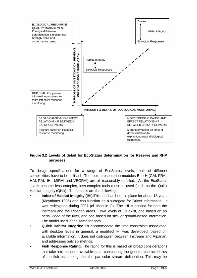
Module A: EcoStatus March 2007 Page A3-6
Figure 3.2 Levels of detail for EcoStatus determination for Reserve and RHP purposes
To design specifications for a range of EcoStatus levels, tools of different complexities have to be utilised. The tools presented in modules B to H (GAI, FRAI, HAI, PAI, IHI, MIRAI and VEGRAI) are all reasonably detailed. As the EcoStatus levels become less complex, less-complex tools must be used (such as the Quick Habitat Integrity (QHI)). These tools are the following: • Index of Habitat Integrity (IHI):This tool has been in place for about 15 years
(Kleynhans 1996) and can function as a surrogate for Driver information. It was redesigned during 2007 (cf. Module G). The IHI is applied for both the Instream and the Riparian areas. Two levels of IHI exist, one based on an aerial video of the river, and one based on site- or ground-based information. The model used is the same for both.
• Quick Habitat Integrity: To accommodate the time constraints associated with desktop levels in general, a modified IHI was developed, based on available information. It does not distinguish between Instream and Riparian, and addresses only six metrics.
• Fish Response Rating: The rating for this is based on broad considerations that take into account available data, considering the general characteristics of the fish assemblage for the particular stream delineation. This may be
ECOLOGICAL RESOURCE QUALITY MANAGEMENT: Ecological Reserve determination & monitoring: Strongly trend-and-conformance based
MORE SPECIFIC CAUSE AND EFFECT RELATIONSHIP BETWEEN BIOTA & DRIVERS:
More informattion on state of drivers (habitat) to explain/understand biological responses.
INTENSITY & DETAIL OF ECOLOGICAL MONITORING
PU
RP
OS
E O
F IN
VE
ST
IGA
TIO
N: R
ES
ER
VE
D
ET
ER
MIN
AT
ION
/ M
ON
ITO
RIN
G
Habitat Integrity
Biological Responses
BROAD CAUSE-AND-EFFECT RELATIONSHIP BETWEEN BIOTA & DRIVERS:
Strongly based on biological response monitoring
RHP, SoR: For general information purposes and more intensive response monitoring
Drivers
Habitat integrity
Biological Responses
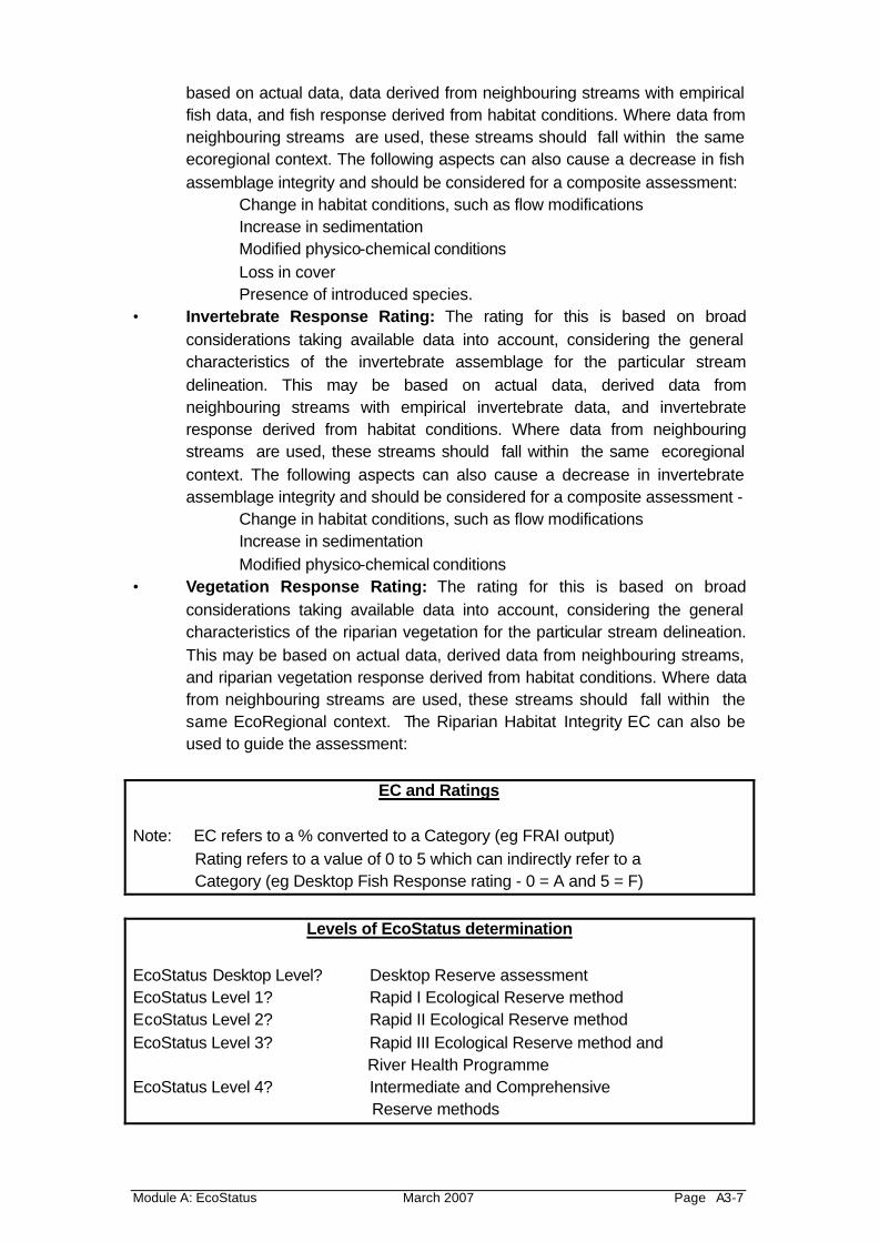
Module A: EcoStatus March 2007 Page A3-7
based on actual data, data derived from neighbouring streams with empirical fish data, and fish response derived from habitat conditions. Where data from neighbouring streams are used, these streams should fall within the same ecoregional context. The following aspects can also cause a decrease in fish assemblage integrity and should be considered for a composite assessment:
Change in habitat conditions, such as flow modifications Increase in sedimentation Modified physico-chemical conditions Loss in cover Presence of introduced species.
• Invertebrate Response Rating: The rating for this is based on broad considerations taking available data into account, considering the general characteristics of the invertebrate assemblage for the particular stream delineation. This may be based on actual data, derived data from neighbouring streams with empirical invertebrate data, and invertebrate response derived from habitat conditions. Where data from neighbouring streams are used, these streams should fall within the same ecoregional context. The following aspects can also cause a decrease in invertebrate assemblage integrity and should be considered for a composite assessment -
Change in habitat conditions, such as flow modifications Increase in sedimentation Modified physico-chemical conditions
• Vegetation Response Rating: The rating for this is based on broad considerations taking available data into account, considering the general characteristics of the riparian vegetation for the particular stream delineation. This may be based on actual data, derived data from neighbouring streams, and riparian vegetation response derived from habitat conditions. Where data from neighbouring streams are used, these streams should fall within the same EcoRegional context. The Riparian Habitat Integrity EC can also be used to guide the assessment:
EC and Ratings
Note: EC refers to a % converted to a Category (eg FRAI output) Rating refers to a value of 0 to 5 which can indirectly refer to a Category (eg Desktop Fish Response rating - 0 = A and 5 = F)
Levels of EcoStatus determination
EcoStatus Desktop Level? Desktop Reserve assessment EcoStatus Level 1? Rapid I Ecological Reserve method EcoStatus Level 2? Rapid II Ecological Reserve method EcoStatus Level 3? Rapid III Ecological Reserve method and
River Health Programme EcoStatus Level 4? Intermediate and Comprehensive
Reserve methods
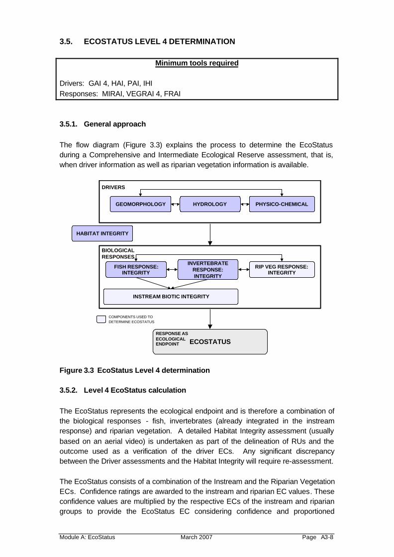
Module A: EcoStatus March 2007 Page A3-8
3.5. ECOSTATUS LEVEL 4 DETERMINATION
Minimum tools required Drivers: GAI 4, HAI, PAI, IHI Responses: MIRAI, VEGRAI 4, FRAI 3.5.1. General approach The flow diagram (Figure 3.3) explains the process to determine the EcoStatus during a Comprehensive and Intermediate Ecological Reserve assessment, that is, when driver information as well as riparian vegetation information is available.
GEOMORPHOLOGY HYDROLOGY PHYSICO-CHEMICAL
FISH RESPONSE: INTEGRITY
INVERTEBRATE RESPONSE: INTEGRITY
RIP VEG RESPONSE: INTEGRITY
HABITAT INTEGRITY
INSTREAM BIOTIC INTEGRITY
ECOSTATUSRESPONSE AS ECOLOGICAL ENDPOINT
DRIVERS
BIOLOGICAL RESPONSES
COMPONENTS USED TO DETERMINE ECOSTATUS
Figure 3.3 EcoStatus Level 4 determination 3.5.2. Level 4 EcoStatus calculation The EcoStatus represents the ecological endpoint and is therefore a combination of the biological responses - fish, invertebrates (already integrated in the instream response) and riparian vegetation. A detailed Habitat Integrity assessment (usually based on an aerial video) is undertaken as part of the delineation of RUs and the outcome used as a verification of the driver ECs. Any significant discrepancy between the Driver assessments and the Habitat Integrity will require re-assessment. The EcoStatus consists of a combination of the Instream and the Riparian Vegetation ECs. Confidence ratings are awarded to the instream and riparian EC values. These confidence values are multiplied by the respective ECs of the instream and riparian groups to provide the EcoStatus EC considering confidence and proportioned

Module A: EcoStatus March 2007 Page A3-9
accordingly. The confidence assessment is done on a similar basis as for the Instream EC (cf 3.3.1) The following figure (taken from the MS Excel spreadsheet) illustrates the procedure (Figure 3.4). NOTE: Only fill in the shaded (grey) cells in spreadsheet / model (see illustrations).
RIPARIAN VEGETATION
EC
%
EC
RIPARIAN VEGETATION ECOLOGICAL CATEGORY 50.0 D
ECOSTATUS
Co
nfi
den
ce
rati
ng
Pro
pori
tons
Mod
ified
w
eig
hts
Confidence rating for instream biological information 3 0.60 38.00Confidence rating for riparian vegetation zone information 2 0.40 20.00
5 1.00 58.00ECOSTATUS C/DEC
Figure 3.4 Illustration of the EcoStatus Level 4 model At this stage of the determination, the information regarding the instream and riparian category and the instream confidence is already available. The confidence rating for riparian vegetation is entered onto the spreadsheet and this will result in calculation the final EcoStatus. The integration of the riparian vegetation EC into the EcoStatus must be carefully considered under particular circumstances. The vegetation could be in much worse condition than the instream biota due to non-flow related sources such as the presence of alien vegetation and/or removal of vegetation. At all times, however, it must be considered whether those attributes of vegetation, specifically in the marginal and lower zone that play a role in the instream integrity, are still functioning. 3.6. ECOSTATUS LEVEL 3 DETERMINATION
Minimum tools required
Drivers: GAI 3, IHI Responses: MIRAI, VEGRAI 3, FRAI
3.6.1. General process The flow diagram (Figure 3.5) explains the process to determine the EcoStatus when applying the Rapid Ecological Reserve Method (Level III) (RERM III) or the River Health Programme. The drivers are assessed in general and not by the driver specialists. Only the instream specialists are involved. An instream specialist that is qualified to undertake the VEGRAI and GAI 3 must be one of the specialists involved.
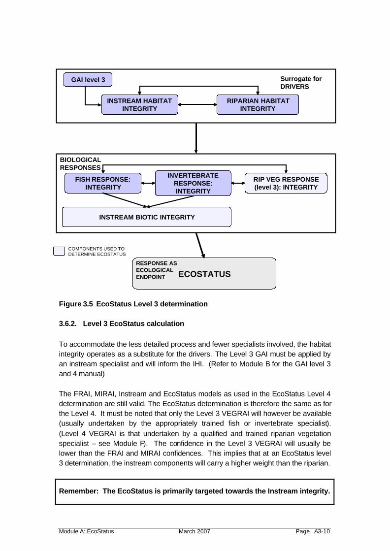
Module A: EcoStatus March 2007 Page A3-10
Figure 3.5 EcoStatus Level 3 determination 3.6.2. Level 3 EcoStatus calculation To accommodate the less detailed process and fewer specialists involved, the habitat integrity operates as a substitute for the drivers. The Level 3 GAI must be applied by an instream specialist and will inform the IHI. (Refer to Module B for the GAI level 3 and 4 manual) The FRAI, MIRAI, Instream and EcoStatus models as used in the EcoStatus Level 4 determination are still valid. The EcoStatus determination is therefore the same as for the Level 4. It must be noted that only the Level 3 VEGRAI will however be available (usually undertaken by the appropriately trained fish or invertebrate specialist). (Level 4 VEGRAI is that undertaken by a qualified and trained riparian vegetation specialist – see Module F). The confidence in the Level 3 VEGRAI will usually be lower than the FRAI and MIRAI confidences. This implies that at an EcoStatus level 3 determination, the instream components will carry a higher weight than the riparian.
Remember: The EcoStatus is primarily targeted towards the Instream integrity.
INSTREAM HABITAT INTEGRITY
RIPARIAN HABITAT INTEGRITY
FISH RESPONSE: INTEGRITY
INVERTEBRATE RESPONSE: INTEGRITY
RIP VEG RESPONSE (level 3): INTEGRITY
INSTREAM BIOTIC INTEGRITY
ECOSTATUSRESPONSE AS ECOLOGICAL ENDPOINT
Surrogate for DRIVERS
BIOLOGICAL RESPONSES
COMPONENTS USED TO DETERMINE ECOSTATUS
GAI level 3

Module A: EcoStatus March 2007 Page A3-11
3.7. ECOSTATUS LEVEL 2, 1 AND DESKTOP DETERMINATION These levels are grouped together as one model, the EcoQuat model (E = EcoStatus and quat = quaternary), which is used for each determination. The EcoQuat model is illustrated in Figure 3.8 and consists of the Quick Habitat Integrity (QHI) Model, the Fish, Invertebrate and Riparian Vegetation Rating and the resulting EcoStatus score. 3.7.1. Desktop EcoStatus
Minimum tools required The basic EcoQuat model is used for the Desktop level which requires the following minimum tools:
Drivers: Quick Habitat Integrity Responses: Fish, Aquatic invertebrate and Riparian vegetation rating
To accommodate the less-detailed process a desktop habitat integrity (using the Quick Habitat Integrity model) that allows for a coarse assessment was developed. This assessment rates the habitat according of a scale of 0 (close to natural) to 5 (critically modified) according to the following metrics :
Bed modification Flow modification Introduced Instream biota Inundation Riparian / bank condition Water quality modification
This Quick Habitat Integrity procedure serves as a substitute for the drivers, as well as playing a role in assessing the EcoStatus. This is necessary because the response information is of low confidence. To accommodate the lack of fish and invertebrate response information, the Quick Habitat Integrity results are brought into the equation to calculate the Instream EC. The Instream EC is therefore a combination of the Quick Habitat Integrity and the Fish and Invertebrate ratings. The riparian vegetation response can be informed by the the riparian / bank condition metrics in the Quick Habitat Integrity. As the EcoStatus is primarily targeted towards the Instream integrity, and as the derived vegetation EC is inherently of lower confidence, the instream EC comprises two thirds of the EcoStatus.

Module A: EcoStatus March 2007 Page A3-12
Figure 3.6 EcoQuat model used for Desktop EcoStatus level (1/3 = proportion of one third , 2/3 = two thirds etc) 3.7.2. EcoStatus Level 1 and 2
The minimum tools required for EcoStatus Level 1 Driver: IHI Responses: Fish, Aquatic Invertebrate and Riparian Vegetation Ratings The only difference from the Desktop EcoStatus Level is the use of the IHI instead of the Quick Habitat Integrity method. The IHI is then used to populate the EcoQuat model using the IHI metric group ratings for the appropriate DHI and other metrics (See Table 3.1) Table 3.1 Links between IHI and EcoQuat Model
ECOQUAT MODEL IHI Bed modification Bed modification metric group (Instream):
Use the highest rating of either of the two metrics (Sediment or benthic growth)
Flow modification Hydrology modification metric (Instream) Inundation Connectivity modification (whichever provides
the highest rating of either the Instream or Riparian)
Bed modification
Flow modification
Introduced biota modification Inundation
Riparian bank condition
Water quality modification
Bed modification
Flow modification
Introduced biota modification Inundation
Riparian bank condition
Water quality modification
QUICK HABITAT INTEGRITY
AVERAGE OF METRICS = QHI
% & EC
FISH RATING INVERTEBRATE RATING
INSTREAM EC
1/3
1/31/3
VEGETATION RATING
ECOSTATUS
1/3
2/3
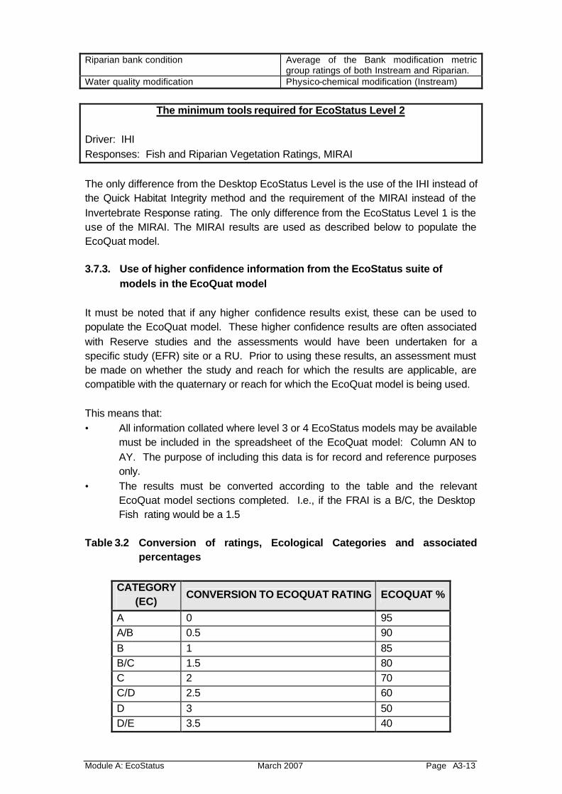
Module A: EcoStatus March 2007 Page A3-13
Riparian bank condition Average of the Bank modification metric group ratings of both Instream and Riparian.
Water quality modification Physico-chemical modification (Instream)
The minimum tools required for EcoStatus Level 2 Driver: IHI Responses: Fish and Riparian Vegetation Ratings, MIRAI The only difference from the Desktop EcoStatus Level is the use of the IHI instead of the Quick Habitat Integrity method and the requirement of the MIRAI instead of the Invertebrate Response rating. The only difference from the EcoStatus Level 1 is the use of the MIRAI. The MIRAI results are used as described below to populate the EcoQuat model. 3.7.3. Use of higher confidence information from the EcoStatus suite of
models in the EcoQuat model It must be noted that if any higher confidence results exist, these can be used to populate the EcoQuat model. These higher confidence results are often associated with Reserve studies and the assessments would have been undertaken for a specific study (EFR) site or a RU. Prior to using these results, an assessment must be made on whether the study and reach for which the results are applicable, are compatible with the quaternary or reach for which the EcoQuat model is being used. This means that: • All information collated where level 3 or 4 EcoStatus models may be available
must be included in the spreadsheet of the EcoQuat model: Column AN to AY. The purpose of including this data is for record and reference purposes only.
• The results must be converted according to the table and the relevant EcoQuat model sections completed. I.e., if the FRAI is a B/C, the Desktop Fish rating would be a 1.5
Table 3.2 Conversion of ratings, Ecological Categories and associated
percentages
CATEGORY (EC)
CONVERSION TO ECOQUAT RATING ECOQUAT %
A 0 95 A/B 0.5 90 B 1 85 B/C 1.5 80 C 2 70 C/D 2.5 60 D 3 50 D/E 3.5 40

Module A: EcoStatus March 2007 Page A3-14
CATEGORY (EC)
CONVERSION TO ECOQUAT RATING ECOQUAT %
E 4 30 E/F 4.5 20 F 5 10
If the RU which the site represents stretches beyond the borders of the quaternary, a decision must be made whether the site is still representative for this quaternary and whether the data can be used. 3.7.4. Comparison of different EcoStatus levels Table 3.3 illustrates the differences between the five EcoStatus levels while Table 3.4 illustrates the use of the different tools usually associated with the different levels. It must be emphasised that, at all levels, the best available information should always be used if applicable for the relevant river reach. More detailed tools than desktop tools can therefore be used if available from other relevant studies (such as detailed hydrology available from water resources planning studies). Table 3.3 Differences between EcoStatus levels in terms of detail addressed.
COMPONENTS Desktop Level 1 Level 2 Level 3 Level 4
DRIVER
Geomorphology GAI 4
Water quality PAI
Hydrology
QHI IHI (instream and riparian)
IHI (instream and riparian)
IHI (instream and riparian) en GAI 3
HAI
RESPONSES
Fish None FRAI FRAI
Invertebrates Rating Rating
MIRAI MIRAI MIRAI
INSTREAM Combination of fish, invert ratings and QHI
Combination of fish, invert ratings and IHI
Combination of fish rating and MIRAI and IHI
FRAI & MIRAI & confidence
FRAI & MIRAI & confidence
Riparian vegetation
Rating Rating Rating VEGRAI 3 VEGRAI 4
ECOSTATUS
EcoStatus
Combination of Instream (2/3) and riparian vegetation (1/3)
Combination of Instream (2/3) and riparian vegetation (1/3)
Combination of Instream (2/3) and riparian vegetation (1/3)
Combination of Instream & VEGRAI. Confidence and weights included
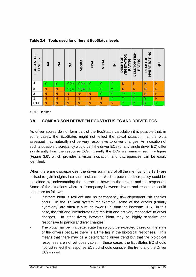
Module A: EcoStatus March 2007 Page A3-15
Table 3.4 Tools used for different EcoStatus levels
EC
OS
TA
TU
S
LE
VE
LS
HA
I
PA
I
GA
I
VE
GR
AI
FRA
I
MIR
AI
IHI
DE
SK
TO
P
VE
GE
TAT
ION
R
AT
ING
DE
SK
TO
P F
ISH
R
AT
ING
DE
SK
TO
P
INV
ER
T R
AT
ING
QH
I
4 Y Y Y (4) Y (4) Y Y Y N N N N
3 N N Y (3) Y (3) Y Y Y N N N N 2 N N N N* N Y Y Y* Y N N 1 N N N N N N Y Y Y Y N DT# N N N N N N N Y Y Y Y
# DT: Desktop 3.8. COMPARISON BETWEEN ECOSTATUS EC AND DRIVER ECS As driver scores do not form part of the EcoStatus calculation it is possible that, in some cases, the EcoStatus might not reflect the actual situation, i.e. the biota assessed may naturally not be very responsive to driver changes. An indication of such a possible discrepancy would be if the driver ECs (or any single driver EC) differ significantly from the response ECs. Usually the ECs are summarised in a figure (Figure 3.6), which provides a visual indication and discrepancies can be easily identified. When there are discrepancies, the driver summary of all the metrics (cf. 3.13.1) are utilised to gain insights into such a situation. Such a potential discrepancy could be explained by understanding the interaction between the drivers and the responses. Some of the situations where a discrepancy between drivers and responses could occur are as follows: • Instream biota is resilient and no permanently flow-dependent fish species
occur. In the Thukela system for example, some of the drivers (usually hydrology) are often in a much lower PES than the instream PES. In this case, the fish and invertebrates are resilient and not very responsive to driver changes. In other rivers, however, biota may be highly sensitive and responsive to particular driver changes.
• The biota may be in a better state than would be expected based on the state of the drivers because there is a time lag in the biological responses. This means that there may be a deteriorating driver trend but that the biological responses are not yet observable. In these cases, the EcoStatus EC should not just reflect the response ECs but should consider the trend and the Driver ECs as well.
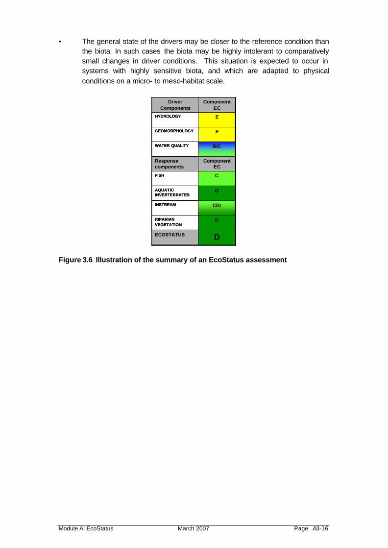
Module A: EcoStatus March 2007 Page A3-16
• The general state of the drivers may be closer to the reference condition than the biota. In such cases the biota may be highly intolerant to comparatively small changes in driver conditions. This situation is expected to occur in systems with highly sensitive biota, and which are adapted to physical conditions on a micro- to meso-habitat scale.
Figure 3.6 Illustration of the summary of an EcoStatus assessment
C/DINSTREAM
DRIPARIAN VEGETATION
DECOSTATUS
DAQUATICINVERTEBRATES
CFISH
Component EC
Response components
B/CWATER QUALITY
EGEOMORPHOLOGY
EHYDROLOGY
Component EC
Driver Components
C/DINSTREAM
DRIPARIAN VEGETATION
DECOSTATUS
DAQUATICINVERTEBRATES
CFISH
Component EC
Response components
B/CWATER QUALITY
EGEOMORPHOLOGY
EHYDROLOGY
Component EC
Driver Components
Module A: EcoStatus March 2007 Page A4-1
4. GUIDANCE IN THE USE OF THE ECOSTATUS LEVEL 4 PROCESS
The EcoStatus model is used in the following ways: • To determine the PES • To derive the Recommended Ecological Category • To derive an alternative Ecological Category • To predict ecological consequences given certain scenarios The rest of this section is provided as guidance for a coordinator / practitioner managing Ecological Water Requirement studies. Note that the Level 3 use is very similar to that of the Level 4. 4.1. DETERMINATION OF THE PES The following provides a step-by-step guidance to apply the EcoStatus Level 4 model at a study site: • The coordinator ensures that all specialists are aware of and understand the
process (specialists should have been exposed to training courses) prior to the first site visit.
• The specialists undertake all required preparatory work prior to going to the field.
• The specialists collate the required information in the field to allow them to complete the respective rule-based models.
• The response specialists require information regarding drivers prior to finalising their rule-based model. The coordinator distributes the rule-based models and information as follows: - Hydrology information to be provided to all specialists. - Geomorphology information to be provided to the riparian vegetation,
fish and invertebrate specialists. - Parallel to this, the physico-chemical information must be provided to
the riparian vegetation, fish and invertebrate specialists. - The vegetation information to be provided to the fish and invertebrate
specialists - Fish and invertebrate specialists to finalise information last and
provide to coordinator. • The aquatic ecologists apply the required weighting to the hydrology and
water quality driver models. • The coordinator obtains the answers to the instream model from the fish and
invertebrate specialists as well as the confidences. • The coordinator finalises the Instream model. • The coordinator obtains the riparian vegetation confidence. • The coordinator runs the EcoStatus model. • In a workshop environment, the weightings are tested with all specialists and
the EcoStatus results finalised. The final results are summarised and
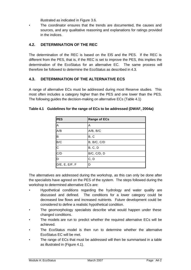
Module A: EcoStatus March 2007 Page A4-2
illustrated as indicated in Figure 3.6. • The coordinator ensures that the trends are documented, the causes and
sources, and any qualitative reasoning and explanations for ratings provided in the indices.
4.2. DETERMINATION OF THE REC The determination of the REC is based on the EIS and the PES. If the REC is different from the PES, that is, if the REC is set to improve the PES, this implies the determination of the EcoStatus for an alternative EC. The same process will therefore be followed to determine the EcoStatus as described in 4.3. 4.3. DETERMINATION OF THE ALTERNATIVE ECS A range of alternative ECs must be addressed during most Reserve studies. This most often includes a category higher than the PES and one lower than the PES. The following guides the decision-making on alternative ECs (Table 4.1) Table 4.1 Guidelines for the range of ECs to be addressed (DWAF, 2004a)
PES Range of ECs
A A
A/B A/B, B/C
B B, C
B/C B, B/C, C/D
C B, C, D
C/D B/C, C/D, D
D C, D
D/E, E, E/F, F D
The alternatives are addressed during the workshop, as this can only be done after the specialists have agreed on the PES of the system. The steps followed during the workshop to determined alternative ECs are: • Hypothetical conditions regarding the hydrology and water quality are
discussed and defined. The conditions for a lower category could be decreased low flows and increased nutrients. Future development could be considered to define a realistic hypothetical condition.
• The geomorphology specialists describe what would happen under these changed conditions.
• The models are run to predict whether the required alternative ECs will be achieved.
• The EcoStatus model is then run to determine whether the alternative EcoStatus EC will be met.
• The range of ECs that must be addressed will then be summarised in a table as illustrated in (Figure 4.1).
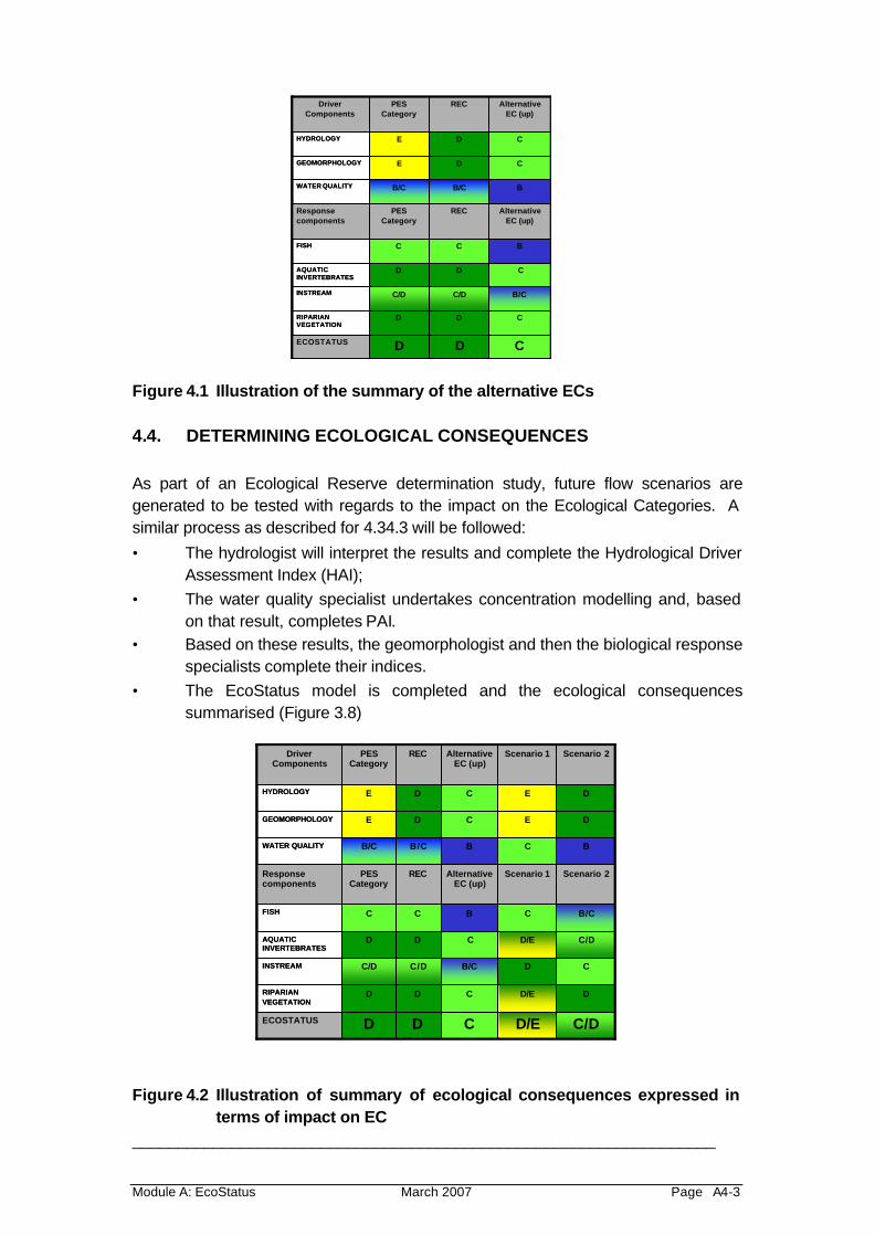
Module A: EcoStatus March 2007 Page A4-3
C
C
B/C
C
B
Alternative EC (up)
B
C
C
Alternative EC (up)
D
D
C/D
D
C
REC
B/C
D
D
REC
D
D
C/D
D
C
PES Category
B/C
E
E
PES Category
INSTREAM
RIPARIAN VEGETATION
ECOSTATUS
AQUATICINVERTEBRATES
FISH
Response components
WATER QUALITY
GEOMORPHOLOGY
HYDROLOGY
Driver Components
C
C
B/C
C
B
Alternative EC (up)
B
C
C
Alternative EC (up)
D
D
C/D
D
C
REC
B/C
D
D
REC
D
D
C/D
D
C
PES Category
B/C
E
E
PES Category
INSTREAM
RIPARIAN VEGETATION
ECOSTATUS
AQUATICINVERTEBRATES
FISH
Response components
WATER QUALITY
GEOMORPHOLOGY
HYDROLOGY
Driver Components
Figure 4.1 Illustration of the summary of the alternative ECs 4.4. DETERMINING ECOLOGICAL CONSEQUENCES As part of an Ecological Reserve determination study, future flow scenarios are generated to be tested with regards to the impact on the Ecological Categories. A similar process as described for 4.34.3 will be followed:
• The hydrologist will interpret the results and complete the Hydrological Driver Assessment Index (HAI);
• The water quality specialist undertakes concentration modelling and, based on that result, completes PAI.
• Based on these results, the geomorphologist and then the biological response specialists complete their indices.
• The EcoStatus model is completed and the ecological consequences summarised (Figure 3.8)
Figure 4.2 Illustration of summary of ecological consequences expressed in
terms of impact on EC _________________________________________________________________
C
C
B/C
C
B
Alternative EC (up)
B
C
C
Alternative EC (up)
D/E
D/E
D
D/E
C
Scenario 1
C
E
E
Scenario 1
C/D
D
C
C/D
B/C
Scenario 2
B
D
D
Scenario 2
D
D
C/D
D
C
REC
B/C
D
D
REC
D
D
C/D
D
C
PES Category
B/C
E
E
PES Category
INSTREAM
RIPARIAN VEGETATION
ECOSTATUS
AQUATICINVERTEBRATES
FISH
Response components
WATER QUALITY
GEOMORPHOLOGY
HYDROLOGY
Driver Components
C
C
B/C
C
B
Alternative EC (up)
B
C
C
Alternative EC (up)
D/E
D/E
D
D/E
C
Scenario 1
C
E
E
Scenario 1
C/D
D
C
C/D
B/C
Scenario 2
B
D
D
Scenario 2
D
D
C/D
D
C
REC
B/C
D
D
REC
D
D
C/D
D
C
PES Category
B/C
E
E
PES Category
INSTREAM
RIPARIAN VEGETATION
ECOSTATUS
AQUATICINVERTEBRATES
FISH
Response components
WATER QUALITY
GEOMORPHOLOGY
HYDROLOGY
Driver Components
Module A: EcoStatus March 2007 Page A5-1
5. REFERENCES
Beechie, RJ, Steel, EA, Roni and Quimby (editors) (2003) Ecosystem recovery planning for listed salmon: an integrated assessment approach for salmon habitat US Dept Commer., NOAA Tech, Memo NMFS-NWFSC-59.183p. Beechie, TJ, and Bolton, S (1999) An approach to restoring salmonid habitat-forming processes in Pacific Northwest watersheds, Fisheries 24(4):6-15. Costanza, R (1992) Towards an operational definition of ecosystem health. In R. Costanza, B. G. Norton, and B. D. Haskell, editors. Ecosystem health: new goals for environmental management. Island Press, Washington, D.C., USA. Department of Water Affairs and Forestry (1999) Resource Directed Measures for Protection of Water Resources., Volume 3: River Ecosystems Version 1.0, Pretoria. Department of Water Affairs and Forestry (2001) DWAF Report No. PB 000-00-5499. Ecological Management Class Report. Prepared by Afridev Consultants and IWR Environmental as part of the Olifants River Ecological Water Requirements Assessment. Department of Water Affairs and Forestry (2004a) DWAF Repot No. PBV000-00-10303. Ecological Reserve Category Report – Reserve Determination Study – Thukela River System. Prepared by IWR Source-to-Sea as part of the Thukela Water Project Decision Support Phase. Department of Water Affairs and Forestry (2004b). DWAF Repot No. PBV000-00-10302. Resource Unit Report – Reserve Determination Study – Thukela River System. Prepared by IWR Source-to-Sea as part of the Thukela Water Project Decision Support Phase. European Commission (2000). Directive 2000/60/EC of the European Parliament and of the Council – Establishing a framework for Community action in the field of water policy. Brussels, Belgium. Iversen, TM, Madsen, BL, and Bøgestrand, J (2000) River conservation in the European Community, including Scandinavia. In: “Global Perspectives on River Conservation: Science Policy and Practice", Edited by P.J. Boon, B.R. Davies and G.E. Petts, John Wiley & Sons Ltd. Joubert, A, 2004 The ecostatus project and mutlicriteria decision analysis: Report and background. Dept of Statistics. University of Cape Town. Prepared for DWAF, RQS.
Module A: EcoStatus March 2007 Page A5-2
Karr, JR, Fausch, KD, Angermeier, PL, Yant PR & Schlosser, LJ (1986) Assessing Biological Integrity in Running Waters: A Method and its Rationale. Special Publication 5, Illinois Natural History Survey, Champaigne. IL. Kleynhans, CJ (1996) A qualitative procedure for the assessment of the habitat integrity status of the Luvuvhu river (Limpopo system, South Africa). Journal of Aquatic Ecosystem Health 5: 41-54 Kleynhans, CJ, Thirion, C, and Moolman, J. (2004). The Development and Refinement of a Level II Ecoregion map for South Africa together with Geomorphological zones for all major Rivers. Project No. 2002-392. Resource Quality Services, Department of Water Affairs and Forestry, Pretoria, South Africa. Louw, MD and Hughes, DA (2002). Prepared for the Department of Water Affairs and Forestry, South Africa. Resource Directed Measures for Protection of Water Resources: River Ecosystems - Revision of a quantity component. Milner, AM (1994) System recovery. In, P.Calow & G.E. Petts (eds.): The rivers handbook. Vol. 2. Blackwell Scientific Publications. London. Nijboer, RC, Johnson, RK, Verdonschot, PFM, Sommerhäuser, M & Buffagni A (2004) Establishing reference conditions for European streams. Hydrobiologia 516: 91–105. Novotny, V,. Bartosova, E, O’Reilly, N & Ehlinger, T (2005). Unlocking the relationship of biotic integrity waters to anthropogenic stresses. Water Research 39: 184-198. Resh, VH, Brown, AV,. Covich, AP,. Gurtz, ME,. Li, HW, Minshall, GW, Reice, SR, Sheldon, AL, Wallace, JB & Wissmar RC (1988) The role of disturbance theory in stream ecology. Journal of the North American Benthological Society. 7: 433-455. Resh, VH, Norris, RH, and Barbour, MT (1995) Design and implementation of rapid assessment approaches for water resource monitoring using benthic macroinvertebrates. Australian Journal of Ecology 20:108-121. Robertson, MP, Villet, MH and Palmer, AR (2004) A fuzzy classification technique for predicting species’ distributions: applications using invasive alien plants and indigenous insects. Diversity and Distributions 10: 461–474. Rogers, KH, & Bestbier, R (1997) Development of a protocol for the definition of the desired state of riverine systems in South Africa. Report on a project executed on behalf of the Department of Environment Affairs and Tourism, Pretoria. Schaeffer, D. J., D. E. Herricks, E. Adwin, and H. W. Kerster. 1988. Ecosystem health: I. Measuring ecosystem health. Environmental Management 12: 445-455.

Module A: EcoStatus March 2007 Page A5-3
U.S. Environmental Protection Agency (2000) Science Policy Council Handbook: Risk Characterization. Washington, DC: Office of Science Policy, Office of Research and Development. EPA 100-B-00-002. Yoder, CO, Miltner, RJ, & White, D (2000) Using biological criteria to assess and classify urban streams and develop improved landscape indicators. Proceedings of the National Conference on Tools for Urban Water Resource Management and Protection, US Environmental Protection Agency, Office Res. Dev., Cincinnati, OH. EPA/625/R-001. __________________________________________________________________