Module 5 Graph Algorithms - Jackson State University

Module 5

Graph Algorithms

Dr. Natarajan Meghanathan

Associate Professor of Computer Science

Jackson State University

Jackson, MS 39217

E-mail: [email protected]

Module Topics

• 5.1 Traversal (DFS, BFS)– Brute Force

• 5.2 Topological Sorting of a DAG– Decrease and Conquer

• 5.3 Single-Source Shortest Path Algorithms (Dijkstra and Bellman-Ford)– Greedy

• 5.4 Minimum Spanning Trees (Prim’s, Kruskal’s)– Greedy

• 5.5 All Pairs Shortest Path Algorithm (Floyd’s)– Dynamic Programming

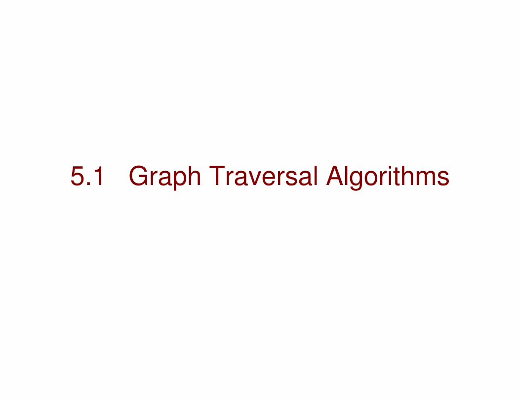
5.1 Graph Traversal Algorithms

Depth First Search (DFS)• Visits graph’s vertices (also called nodes) by always moving away

from last visited vertex to unvisited one, backtracks if there is no adjacent unvisited vertex.

• Break any tie to visit an adjacent vertex, by visiting the vertex with the lowest ID or the lowest alphabet (label).

• Uses a stack

– a vertex is pushed onto the stack when it’s visited for the first time

–a vertex is popped off the stack when it becomes a dead end, i.e., when there is no adjacent unvisited vertex

• “Redraws” graph in tree-like fashion (with tree edges andback edges for undirected graph):

– Whenever a new unvisited vertex is reached for the first time, it is attached as a child to the vertex from which it is being reached. Such an edge is called a tree edge.

– While exploring the neighbors of a vertex, it the algorithm encounters an edge leading to a previously visited vertex other than its immediate predecessor (i.e., its parent in the tree), such an edge is called a back edge.

– The leaf nodes have no children; the root node and other intermediate nodes have one more child.

Pseudo Code of DFS

Example 1: DFS

Source: Figure 3.10: Levitin, 3rd Edition: Introduction to the Design and Analysis of Algorithms,

2012.

DFS• DFS can be implemented with graphs represented as:

–adjacency matrices: Θ(V2); adjacency lists: Θ(|V|+|E|)

• Yields two distinct ordering of vertices:–order in which vertices are first encountered (pushed onto stack)

–order in which vertices become dead-ends (popped off stack)

• Applications:–checking connectivity, finding connected components

• The set of vertices that we can visit through DFS, starting from a particular vertex in the set constitute a connected component.

• If a graph has only one connected component, we need to run DFS only once and it returns a tree; otherwise, the graph has more than one connected component and we determine a forest – comprising of trees for each component.

–checking for cycles (a DFS run on an undirected graph returns a back edge)

–finding articulation points and bi-connected components• An articulation point of a connected component is a vertex that when

removed disconnects the component.

• A graph is said to have bi-connected components if none of its components have an articulation point.

Example 2: DFS

f b c g

d a e

f b c g

d a e

1, 7

2, 3

3, 2

4, 1 5, 6 6, 5

7, 4

Tree Edge

Back Edge

• Notes on Articulation Point– The root of a DFS tree is an articulation point if it has more than

one child connected through a tree edge. (In the above DFS tree,the root node ‘a’ is an articulation point)

– The leaf nodes of a DFS tree are not articulation points.

– Any other internal vertex v in the DFS tree, if it has one or more sub trees rooted at a child (at least one child node) of v that does NOT have an edge which climbs ’higher ’ than v (through a back edge), then v is an articulation point.

DFS: Articulation Points

• In the above graph, vertex ‘a’ is the only articulation point.

• Vertices ‘e’ and ‘f’ are leaf nodes.

• Vertices ‘b’ and ‘c’ are candidates for articulation points. But, they cannot become articulation point, because there is a back edge from the only sub tree rooted at their child nodes (‘d’ and ‘g’ respectively) that have a back edge to ‘a’.

• By the same argument, vertices ‘d’ and ‘g’ are not articulation points, because they have only child node (f and e respectively); each of these child nodes are connected to a higher level vertex (b and a respectively) through a back edge.

a

b c

d

f

g

e

Based on

Example 2

Example 3: DFS and Articulation Points

f b c g

d a e

f b c g

d a e

1, 7

2, 3

3, 2

4, 1 5, 6 6, 5

7, 4

Tree Edge

• In the above new graph (different from the previous example: note edges b –f, a – d and a – e are missing), vertices ‘a’, ‘b’, ‘c’, ‘d’ and ‘g’ are articulation points, because:– Vertex ‘a’ is the root node of the DFS tree and it has more than one child

node– Vertex ‘b’ is an intermediate node; it has one sub tree rooted at its child node

(d) that does not have any node, including ‘d’, to climb higher than ‘b’. So, vertex ‘b’ is an articulation point.

– Vertex ‘c’ is also an articulation point, by the same argument as above – this time, applied to the sub tree rooted at child node ‘g’.

– Vertices ‘d’ and ‘g’ are articulation points; because, they have one child node (‘f’ and ‘e’ respectively) that are not connected to any other vertex higher than ‘d’ and ‘g’ respectively.


f b c g

d a e

f b c g

d a e

1, 7

2, 3

3, 2

4, 1 5, 6 6, 5

7, 4

Tree Edge

• In the above new graph (different from the previous example: note edge a – e and b – f are added back; but a – d is missing):– Vertices ‘a’ and ‘b’ are

articulation points

– Vertex ‘c’ is not an articulation point

Back Edge

a

b c

d

f

g

e


a

b

c

d e

f g

h

i j

k

a

b

c

d e

f g

h

i j

k

DFS TREE

1) Root Vertex ‘a’ has more than one child; so, it is an articulation point.2) Vertices ‘d’, ‘g’ and ‘j’ are leaf nodes3) Vertex ‘b’ is not an articulation point becausethe only sub tree rooted at its child node ‘c’ hasa back edge to a vertex higher than ‘b’ (in thiscase to the root vertex ‘a’)4) Vertex ‘c’ is an articulation point. One of itschild vertex ‘d’ does not have any sub tree rooted at it. The other vertex ‘e’ has a sub tree rooted at it and this sub tree has noback edge higher up than ‘c’. 5) By argument (4), it follows that vertex ‘e’is not an articulation point because the sub treerooted at its child node ‘f’ has a back edge higherup than ‘e’ (to vertex ‘c’); 6) Vertices ‘f’ and ‘k’ are not articulation points becausethey have only one child node each and the child nodesare connected to a vertex higher above ‘f’ and ‘k’.7) Vertex ‘i’ is not an articulation point because the only sub tree rooted at its child has a back edge higher up (to vertices ‘a’ and ‘h’). 8) Vertex ‘h’ is not an articulation point because the only sub tree rooted at ‘h’ has a back edge higher up (to the root vertex ‘a’).

Identification of the Articulation Points of the Graph in Example 5

a

b

c

d e

f g

h

i j

k

Breadth First Search (BFS)• BFS is a graph traversal algorithm (like DFS); but, BFS proceeds in a

concentric breadth-wise manner (not depth wise) by first visiting all the vertices that are adjacent to a starting vertex, then all unvisited vertices that are two edges apart from it, and so on.– The above traversal strategy of BFS makes it ideal for determining

minimum-edge (i.e., minimum-hop paths) on graphs.

• If the underling graph is connected, then all the vertices of the graph should have been visited when BFS is started from a randomly chosen vertex. – If there still remains unvisited vertices, the graph is not connected and the

algorithm has to restarted on an arbitrary vertex of another connected component of the graph.

• BFS is typically implemented using a FIFO-queue (not a LIFO-stack like that of DFS).– The queue is initialized with the traversal’s starting vertex, which is marked

as visited. On each iteration, BFS identifies all unvisited vertices that are adjacent to the front vertex, marks them as visited, and adds them to the queue; after that, the front vertex is removed from the queue.

• When a vertex is visited for the first time, the corresponding edge that facilitated this visit is called the tree edge. When a vertex that is already visited is re-visited through a different edge, the corresponding edge is called a cross edge.

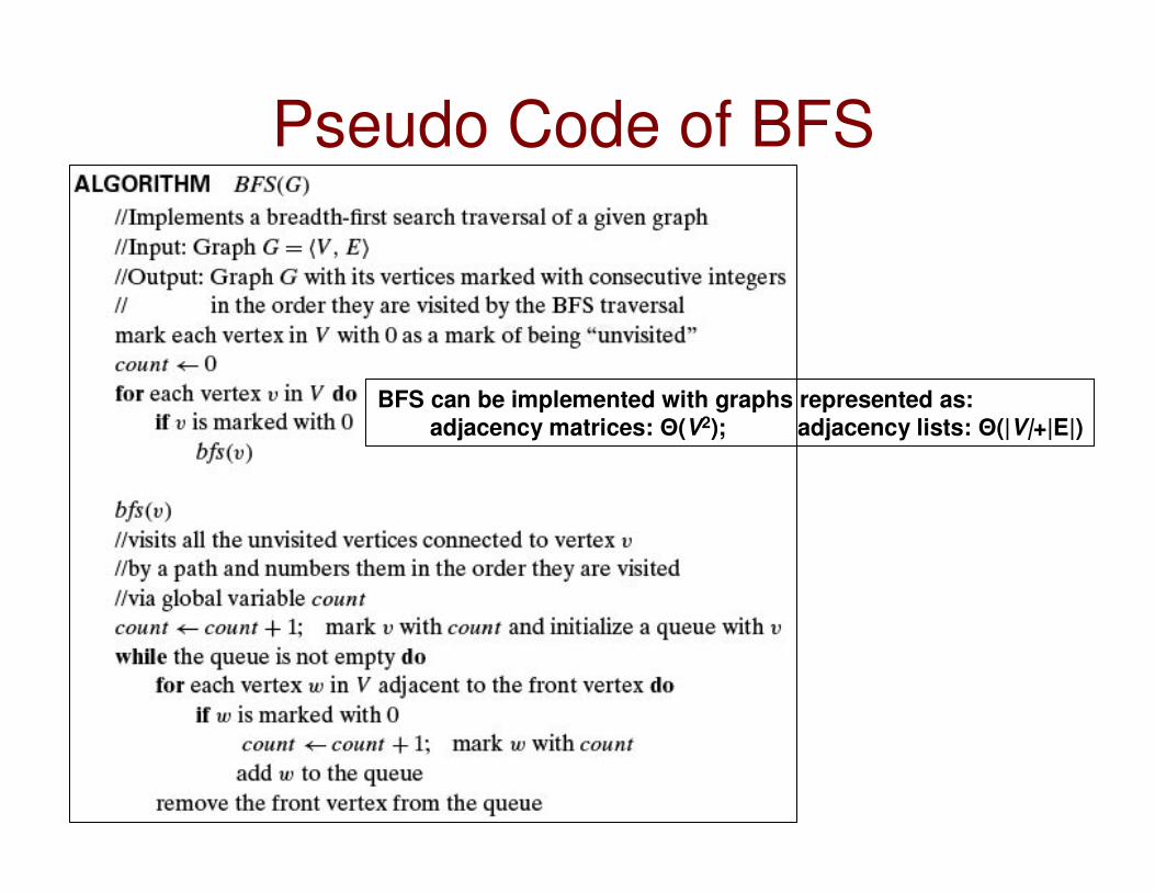
Pseudo Code of BFS

BFS can be implemented with graphs represented as:adjacency matrices: Θ(V2); adjacency lists: Θ(|V|+|E|)

Example for BFS


2012.

0

1 1 1

2 2

0

1 1

2

Use of BFS to find Minimum Edge Paths


2012.

Note: DFS cannot be used to find minimum edge paths, because DFS is not guaranteed to visit all the one-hop neighbors of a vertex, before visiting its two-hop neighbors and so on.

For example, if DFS is executed starting from vertex ‘a’ on the above graph, then vertex ‘e’would be visited through the path a – b – c – d – h – g – f – e and not through the direct path a – e, available in the graph.

a b c d

e f g h

1 2

3

5

4

7

6

8

Comparison of DFS and BFS

Source: Table 3.1: Levitin, 3rd Edition: Introduction to the Design and Analysis of Algorithms,

2012.

With the levels of a tree, referenced starting from the root node, A back edge in a DFS tree could connect vertices at different levels; whereas, a cross edgein a BFS tree always connects vertices that are either at the same level or at adjacent levels.

There is always only a unique ordering of the vertices, according to BFS, in the order they are visited (added and removed from the queue in the same order). On the other hand, with DFS – vertices could be ordered in the order they are added to the Stack, typically different from the order in which they are removed from the stack.

Bi-Partite (2-Colorable) Graphs • A graph is said to be bi-partite or 2-colorable if the vertices of the

graph can be colored in two colors such that every edge has its vertices in different colors.

• In other words, we can partition the set of vertices of a graph into two disjoint sets such that there is no edge between vertices in the same set. All the edges in the graph are between vertices from the two sets.

• We can check for the 2-colorable property of a graph by running a DFS or BFS– With BFS, if there are no cross-edges between vertices at the same level,

then the graph is 2-colorable.

– With DFS, if there are no back edges between vertices that are both at odd levels or both at even levels, then the graph is 2-colorable.

• We will use BFS as the algorithm to check for the 2-colorability of a graph.– The level of the root is 0 (consider 0 to be even).

– The level of a child node is 1 more than the level of the parent node from which it was visited through a tree edge.

– If the level of a node is even, then color the vertex in yellow.

– If the level of a node is odd, then color the vertex in green.

Bi-Partite (2-Colorable) Graphs

a b c

d e f

a b c

d e f

0 1

1

2

2 3

a b c

d e f

Example for a 2-Colorable Graph

a b

d e

Example for a Graph that is Not 2-Colorable

a b

d e

0 1

1 1

We encounter cross edges between vertices

b and e; d and e – all the three vertices are

in the same level.

Examples: 2-Colorability of Graphs

f b c g

d a e

f b c g

d a e

01

1

1

1

b – d is a cross edge between

Vertices at the same level. So,

the graph is not 2-colorable

f b c g

d a e

f b c g

d a e

0

11

1

2

2

2

The above graph is 2-Colorable

as there are no cross edges

between vertices at the same level

5.2 Topological Sort

DFS: Edge Terminology for directed

graphsa b

c

d

e

a b

c

d

e

Tree edge

Back edge

Forward edge

Cross edge

Tree edge – an edge from a parent node to a child node in the tree

Back edge – an edge from a vertex to its ancestor node in the tree

Forward edge – an edge from an ancestor node to its descendant node in the tree.

The two nodes do not have a parent-child relationship. The back and forward

edges are in a single component (the DFS tree). Cross edge – an edge between two different components of the DFS Forest. So, basically an edge other than a tree edge, back edge and forward edge

1, 3 2, 2

3, 1

4, 5

5, 4

Directed Acyclic Graphs (DAG)• A directed graph is a graph with directed edges between

its vertices (e.g., u � v).

• A DAG is a directed graph (digraph) without cycles.

– A DAG is encountered for many applications that

involve pre-requisite restricted tasks (e.g., course

scheduling)

a b

c d

a b

c d

a a

DAGDAG

not a not a

DAGDAG

To test whether a directed graph is a DAG, run DFS on the directed graph. If a

back edge is not encountered, then the directed graph is a DAG.

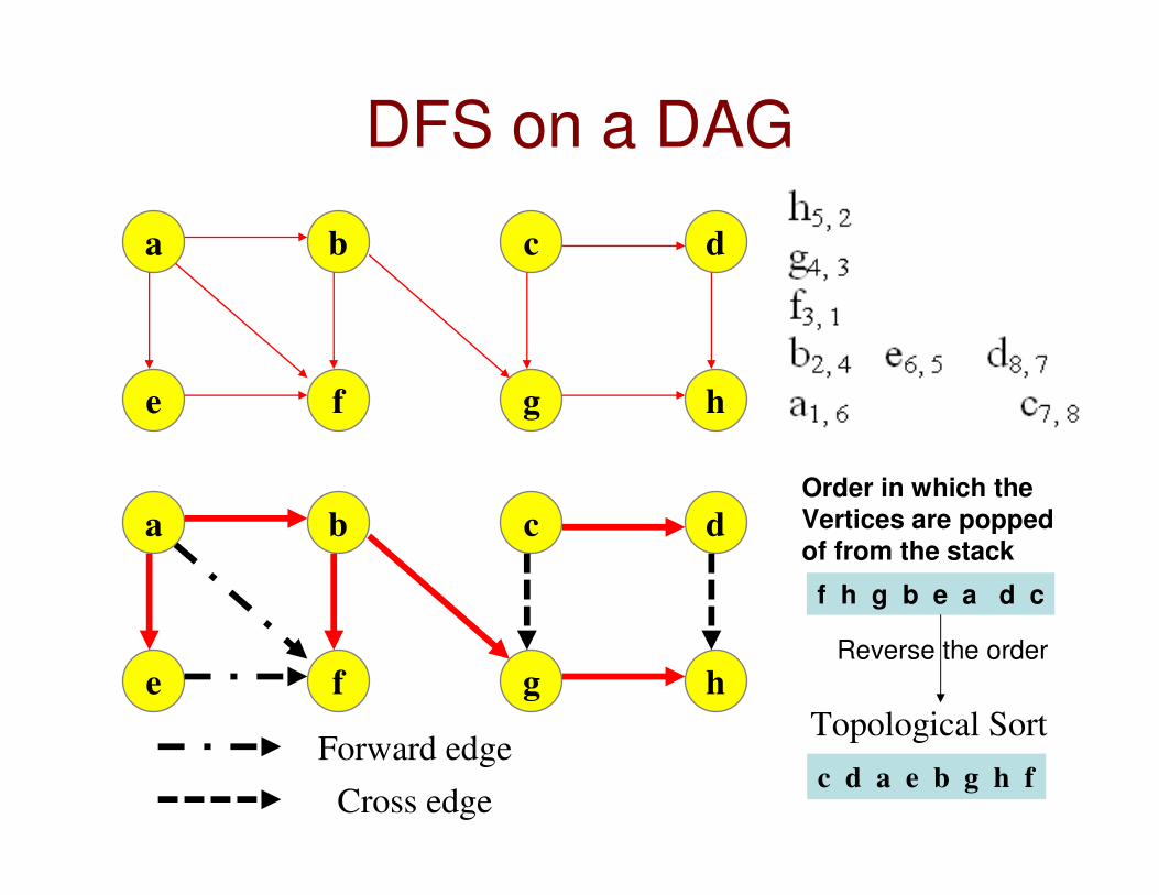
DFS on a DAG

a b

e f

c d

g h

a b

e f

c d

g h

Forward edgeTopological Sort

c d a e b g h f

f h g b e a d c

Order in which the

Vertices are popped

of from the stack

Reverse the order

Cross edge

Topological Sort• Topological sort is an ordering of the vertices of a directed

acyclic graph (DAG) – a directed graph (a.k.a. digraph) without cycles.– This implies if there is an edge u� v in the digraph, then u should

be listed ahead of v in the topological sort: … u … v …

– Being a DAG is the necessary and sufficient condition to be able to do a topological sorting for a digraph.

– Proof for Necessary Condition: If a digraph is not a DAG and lets say it has a topological sorting. Consider a cycle (in the digraph) comprising of vertices u1, u2, u3, …, uk, u1. In other words, there is an edge from uk to u1 and there is a directed path to uk from u1. So, it is not possible to decide whether u1 should be ahead of uk or after uk in the topological sorting of the vertices of the digraph. Hence, there cannot be a topological sorting of thevertices of a digraph, if the digraph has even one cycle. To be able to topologically sort the vertices of a digraph, the digraph hasto first of all be a DAG. [Necessary Condition]. We will next prove that this is also the sufficient condition.

Topological SortProof for Sufficient Condition

• After running DFS on the digraph (also a DAG), the topological sorting is the listing of the vertices of the DAG inthe reverse order according to which they are removed from the stack. – Consider an edge u � v in the digraph (DAG).

– If there exists, an ordering that lists v ahead of u, then it implies that u was popped out from the stack ahead of v. That is, vertex v has been already added to the stack and we were to able to visit vertex u by exploring a path leading from v to u. This means the edge u �

v has to be a back edge. This implies, the digraph has a cycle and is not a DAG. We had earlier proved that if a digraph has a cycle, we cannot generate a topological sort of its vertices.

– For an edge u->v, if v is listed ahead of u ==> the graph is not a DAG (Note that a ==> b, then !b ==> !a)

– If the graph is a DAG ==> u should be listed ahead of v for every edge u � v.

– Hence, it is sufficient for a directed to be DAG to generate a topological sort for it.

5.3 Dijkstra’s Shortest Path Algorithm

Shortest Path (Min. Wt. Path) Problem

• Path p of length k from a vertex s to a vertex d is a sequence (v0, v1, v2, …, vk) of vertices such that v0 = sand vk = d and (vi-1, vi) Є E, for i =1, 2,…, k

• Weight of a path p = (v0, v1, v2, …, vk) is

• The weight of a shortest path from s to d is given by

δ(s, d) = min {w(p): s d if there is a path from s to d}

= ∞ otherwise

Examples of shortest path-finding algorithms:

• Dijkstra algorithm – Θ(|E|*log|V|)

• Bellman-Ford algorithm – Θ(|E|*|V|)

∑=

−=

k

i

ii vvwpw1

1 ),()(

p

Dijkstra Algorithm• Assumption: w (u, v) >= 0 for each edge (u, v) Є E

• Objective: Given G = (V, E, w), find the shortest weight path

between a given source s and destination d

• Principle: Greedy strategy

• Maintain a minimum weight path estimate d [v] from s to each other

vertex v.

• At each step, pick the vertex that has the smallest minimum weight

path estimate

• Output: After running this algorithm for |V| iterations, we get the

shortest weight path from s to all other vertices in G

• Note: Dijkstra algorithm does not work for graphs with edges (other

than those leading from the source) with negative weights.

31

Principle of Dijkstra Algorithm

0 Ws-u

Ws-v

Path from s to u

s u

W(u

, v)

If Ws-v > Ws-u + W(u, v) then

Ws-v = Ws-u + W(u, v)

Predecessor (v) = u

else

Retain the current path from s to v

Principle in a nutshell

During the beginning of each iteration we

will pick a vertex u that has the minimum

weight path to s. We will then explore

the neighbors of u for which we have not

yet found a minimum weight path. We will

try to see if by going through u, we can

reduce the weight of path from s to v,

where v is a neighbor of u.

v

Note: Sub-path of a shortest path is also a shortest path. For example, if

s – a – c – f – g – d is the minimum weight path from s to d, then c – f – g – d

and a – c – f – g are the minimum weight paths from c to d and a to g respectively.

Relaxation Condition

32

Dijkstra AlgorithmBegin Algorithm Dijkstra (G, s)

1 For each vertex v Є V

2 d [v] ← ∞ // an estimate of the min-weight path from s to v

3 End For

4 d [s] ← 0

5 S ← Φ // set of nodes for which we know the min-weight path from s

6 Q ← V // set of nodes for which we know estimate of min-weight path from s

7 While Q ≠ Φ

8 u ← EXTRACT-MIN(Q)

9 S ← S U {u}

10 For each vertex v such that (u, v) Є E

11 If v Q and d [v] > d [u] + w (u, v) then

12 d [v] ← d [u] + w (u, v)

13 Predecessor (v) = u

13 End If

14 End For

15 End While

16 End Dijkstra

∈

33

Dijkstra Algorithm: Time ComplexityBegin Algorithm Dijkstra (G, s)



3 End For

4 d [s] ← 0

5 S ← Φ // set of nodes for which we know the min-weight path from s

6 Q ← V // set of nodes for which we know estimate of min-weight path from s

7 While Q ≠ Φ


9 S ← S U {u}


11 If v Q and d [v] > d [u] + w (u, v) then

12 d [v] ← d [u] + w (u, v)


13 End If

14 End For

15 End While

16 End Dijkstra

∈

Θ(V) time

Θ(V) time to

Construct a

Min-heap

done |V| times = Θ(V) time

Each extraction takes Θ(logV) time

done Θ(E) times totally

It takes Θ(logV) time when

done once

Overall Complexity: Θ(V) + Θ(V) + Θ(VlogV) + O(ElogV)

Since |V| = O(|E|), the VlogV term is dominated by the

ElogV term. Hence, overall complexity = O(|E|*log|V|)

Dijkstra Algorithm (Example 1)

∞∞0

∞∞∞

3 5

54

2

1

3

13

s

uv

wx

y

∞30

∞54

35

54

2

1

3

13

s

uv

wx

y

830

644

35

54

2

1

3

13

s

uv

wx

y

830

644

3 5

54

2

1

3

13

s

uv

wx

yv v

(a) (b) (c)

(d) (e) (f)

830

644

3 5

54

2

1

3

13

s

u

wx

y

730

644

3 5

54

2

1

3

13

s

u

wx

y

35

0

∞ ∞

∞

∞ ∞

5

7

6

1

3

2

4

3

Initial

A

B D

F

C E

0

5 ∞

∞

3 ∞

5

7

6

1

3

2

4

3

Iteration 1

A

B D

F

C E

0

4 ∞

∞

3 7

5

7

6

1

3

2

4

3

Iteration 2

A

B D

F

C E

0

4 11

∞

3 7

5

7

6

1

3

2

4

3

Iteration 3

A

B D

F

C E

0

4 9

10

3 7

5

7

6

1

3

2

4

3

Iteration 4

A

B D

F

C E

0

4 9

10

3 7

5

7

6

1

3

2

4

3

Iteration 5

A

B D

F

C E

0

4 9

10

3 7

1

3

2

4

3Shortest Path Tree

A

B D

F

C E

Dijkstra Algorithm

Example 2

36

0 ∞ ∞

∞ ∞ ∞

A B C

DEF

5 6

8 5

3 31 2 2

Initial

0 5 ∞

3 ∞ ∞

A B C

DEF

5 6

8 5

3 31 2 2

Iteration 1

0 4 ∞

3 11 ∞

A B C

DEF

5 6

8 5

3 31 2 2

Iteration 2

0 4 10

3 6 6

A B C

DEF

5 6

8 5

3 31 2 2

Iteration 3

0 4 9

3 6 6

A B C

DEF

5 6

8 5

3 31 2 2

Iteration 4

0 4 9

3 6 6

A B C

DEF

5 6

8 5

3 31 2 2

Iteration 5

0 4 9

3 6 6

A B C

DEF

3 31 2 2

Shortest Path Tree

Dijkstra Algorithm Example 3

Theorems on Shortest Paths and Dijsktra Algorithm

• Theorem 1: Sub path of a shortest path is also shortest.

• Proof: Lets say there is a shortest path from s to d through the vertices s –a – b – c – d.

• Then, the shortest path from a to c is also a – b – c.

• If there is a path of lower weight than the weight of the path from a – b – c, then we could have gone from s to d through this alternate path from a to c of lower weight than a – b – c.

• However, if we do that, then the weight of the path s – a – b – c – d is not the lowest and there exists an alternate path of lower weight.

• This contradicts our assumption that s – a – b – c – d is the shortest (lowest weight) path.

• Theorem 2: When a vertex v is picked for relaxation/optimization, every intermediate vertex on the s…v shortest path is already optimized.

• Proof: Let there be a path from s to v that includes a vertex x (i.e., s...x...v) for which we have not yet found the shortest path. From Theorem 1, weight(s...x) < weight(s...v). Also, the x...v path has to have edges of positive weight. Then, the Dijkstra's algorithm would have picked up xahead of v. So, the fact that we picked v as the vertex with the lowest weight among the remaining vertices (yet to be optimized) implies that every intermediate vertex on the s...v is already optimized.

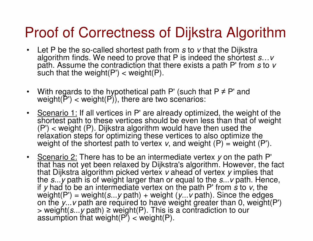
Proof of Correctness of Dijkstra Algorithm• Let P be the so-called shortest path from s to v that the Dijkstra

algorithm finds. We need to prove that P is indeed the shortest s…vpath. Assume the contradiction that there exists a path P' from s to v such that the weight(P') < weight(P).

• With regards to the hypothetical path P' (such that P ≠ P' and weight(P') < weight(P)), there are two scenarios:

• Scenario 1: If all vertices in P' are already optimized, the weight of the shortest path to these vertices should be even less than that of weight (P') < weight (P). Dijkstra algorithm would have then used the relaxation steps for optimizing these vertices to also optimize the weight of the shortest path to vertex v, and weight (P) = weight (P').

• Scenario 2: There has to be an intermediate vertex y on the path P' that has not yet been relaxed by Dijkstra's algorithm. However, the fact that Dijkstra algorithm picked vertex v ahead of vertex y implies that the s...y path is of weight larger than or equal to the s...v path. Hence, if y had to be an intermediate vertex on the path P' from s to v, the weight(P') = weight(s...y path) + weight (y...v path). Since the edges on the y...v path are required to have weight greater than 0, weight(P') > weight(s...y path) ≥ weight(P). This is a contradiction to our assumption that weight(P') < weight(P).

Proof of Correctness of Dijkstra Algorithm• Let P be the so-called shortest path from s to v that the Dijkstra

algorithm finds. We need to prove that P is indeed the shortest s…vpath. Assume the contradiction that there exists a path P' from s to v such that the weight(P') < weight(P). We will now explore whether such a hypothetical path P’ can exist.

• We claim that there should be at least one intermediate vertex on the path P’ that is not yet optimized; because if every intermediate vertexon path P’ were already optimized, we could have found the path P’through the sequence of relaxations of the intermediate nodes on P’and since weight(P’) < weight(P), we would have chosen P’ instead of P as the shortest path, as part of the Dijkstra algorithm. We did not do so.

• Thus, if there is at least one intermediate vertex (say u’) on P’ and is not yet optimized, the weight of the path from s to u’ should have been greater than or equal to the weight of the path from s to v (otherwise, the Dijkstra algorithm would have picked u’ instead of v for optimization). Since all edge weights are positive, the weight of the path P’ (comprising of the edges from s to u’ and then from u’ to v) would be definitely greater than the weight of the path P from s to v. This is a contradiction. Hence, the path found by the Dijkstra algorithm is the shortest path.

Bellman-Ford Algorithm• Used to find single source shortest path trees on any

graph (including those with negative weight edges).

• Starts with an estimate of 0 for the source and ∞ as estimates for the shortest path weights from the source to every other vertex; we proceed in iterations:– In each iteration, we relax every vertex (instead of just one

vertex, as in Dijkstra) and try to improve the estimates of the shortest path weights to the neighbors

– We do not target to optimize any particular vertex in an iteration; but since there cannot be more than V – 1 intermediate edges on path from the source to any vertex, we proceed for a total of

V – 1 iterations for a graph of V vertices.

– The time complexity is Θ(VE)

– Optimization: In a particular iteration, if the estimates of theshortest path weights does not change for even one vertex, then we could stop!

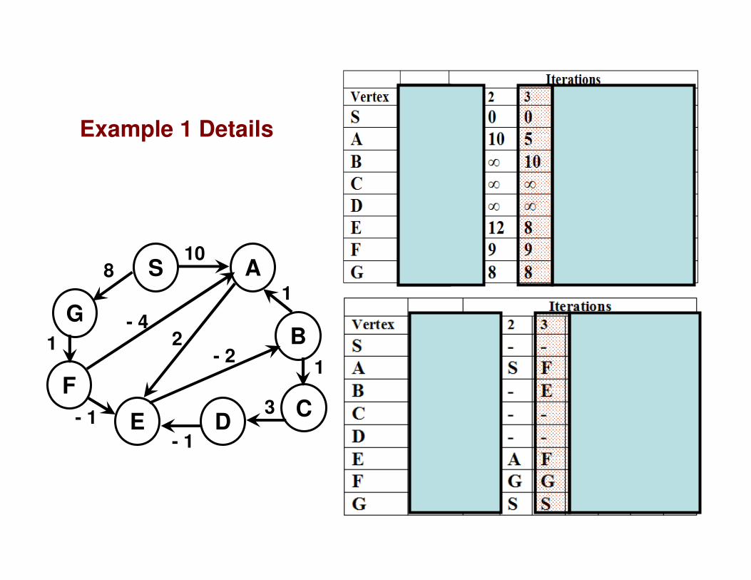
Bellman-Ford Algorithm Example 1S A

GB

CDE

F

108

1

- 1

- 42

- 2

- 1

3

1

1

S A

GB

CDE

F

8

1- 4

2- 2

3

1

S A

GB

CDE

F

108

1

- 1

- 42

- 2

- 1

3

1

1

Example 1 Details

S A

GB

CDE

F

108

1

- 1

- 42

- 2

- 1

3

1

1

Example 1 Details

S A

GB

CDE

F

8

1- 4

2- 2

3

1

Bellman-Ford Algorithm Example 2

A

B D

F

C E

7

5

1

43

6

3

2

A

B D

F

C E

1

43 3

2

5.4 Minimum Spanning Trees

53

Minimum Spanning Tree Problem• Given a weighted graph, we want to determine a tree that spans all

the vertices in the tree and the sum of the weights of all the edges in such a spanning tree should be minimum.

• Two algorithms:– Prim algorithm: Θ(|E|*log|V|),

– Kruskal Algorithm: Θ(|E|*log |E| + |V|*log|V|))

• Prim algorithm is just a variation of Dijkstra algorithm with the relaxation condition beingIf v Q and d [v] > w (u, v) then

d [v] ← w (u, v)

Predecessor (v) = u

End If

• Kruskal algorithm: Consider edges in the increasing order of their weights and include an edge in the tree, if and only if, by including the edge in the tree, we do not create a cycle!!

• Note: Shortest Path trees need not always have minimum weight and minimum spanning trees need not always be shortest path trees.

On each iteration, the algorithm expands the

current tree in a greedy manner by attaching to

it the nearest vertex not in the tree. By the

‘nearest vertex’, we mean a vertex not in the

tree connected to a vertex in the tree by an

edge of the smallest weight.

∈

Properties of Minimum Spanning Tree• Property 1: If an edge (i, j) is part of a minimum spanning tree T of a

weighted graph of V vertices, its two end vertices are part of an IJ-cut and (i, j) is the minimum weight edge in the IJ-cut-set.

• Proof: We will prove this by contradiction. Assume an edge (i, j) exists

in a minimum spanning tree T. Let there be an edge (i', j') of an IJ-cut

such that vertices i and i' are in I and vertices j and j' are in J, and that

weight(i', j') < weight(i, j). If that is the case, we can remove (i, j) from

the minimum spanning tree T and restore its connectivity and spanning

nature by adding (i', j') instead. By doing this, we will only lower the

weight of T contradicting the assumption that T is a minimum spanning

tree to start with. Hence, every edge (i, j) of a minimum spanning tree

has to be the minimum weight edge in an IJ-cut such that i is in I and j is

in J, and I U J = V and I n J = ϕ.

55

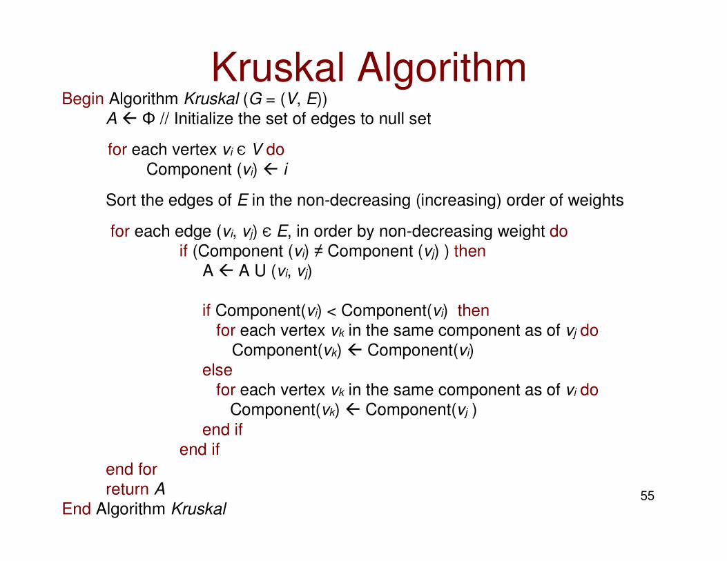
Kruskal AlgorithmBegin Algorithm Kruskal (G = (V, E))

A Φ // Initialize the set of edges to null set

for each vertex vi Є V do

Component (vi) i

Sort the edges of E in the non-decreasing (increasing) order of weights

for each edge (vi, vj) Є E, in order by non-decreasing weight do

if (Component (vi) ≠ Component (vj) ) then

A A U (vi, vj)

if Component(vi) < Component(vi) then

for each vertex vk in the same component as of vj do

Component(vk) Component(vi)

else

for each vertex vk in the same component as of vi do

Component(vk) Component(vj )

end if

end if

end for

return A

End Algorithm Kruskal

56

Kruskal Algorithm: Time ComplexityBegin Algorithm Kruskal (G = (V, E))

A Φ // Initialize the set of edges to null set

for each vertex vi Є V do

Component (vi) i

Sort the edges of E in the non-decreasing (increasing) order of weights

for each edge (vi, vj) Є E, in order by non-decreasing weight do

if (Component (vi) ≠ Component (vj) ) then

A A U (vi, vj)

if Component(vi) < Component(vi) then

for each vertex vk in the same component as of vj do

Component(vk) Component(vi)

else

for each vertex vk in the same component as of vi do

Component(vk) Component(vj )

end if

end if

end for

return A

End Algorithm Kruskal

Takes

Θ(logV)

time per

merger

Can be done in

Θ(logV) time

V-1 mergers.

So, Θ(VlogV)

Θ(V) time

Θ(ElogE)

time

Overall time complexity:

Θ(V) + Θ(ElogE) + Θ(VlogV) = Θ(VlogV + ElogE)

Components are kept track of using

a Disjoint-set data structure

57

Kruskal Algorithm (Example 1)

xws

yvu

3 5

54

2

1

3

13

s

uv

wx

y

(a) (b) (c)

(d) (e) (f)

Weight of the minimum spanning tree = 10

Weight of the shortest path tree = 12

xvs

yvu

3 5

54

2

1

3

13

s

uv

wx

y

xvs

xvu

3 5

54

2

1

3

13

s

uv

wx

y

xus

xuu

3 5

54

2

1

3

13

s

uv

wx

y

uus

uuu

3 5

54

2

1

3

13

s

uv

wx

y

sss

sss

3 5

54

2

1

3

13

s

uv

wx

y

58

AA BB

C

C

DDE E

FFG G

5

7

9

8

75

15

68

11

9

Initial Kruskal Algorithm

Example 2 for

Minimum Spanning

Tree

AA BB

C

C

ADE E

FFG G

5

7

9

8

75

15

68

11

9

Iteration 1

AA BB

C

C

ADC E

FFG G

5

7

9

8

75

15

68

11

9

Iteration 2

AA BB

C

C

AD C E

AFG G

5

7

9

8

75

15

68

11

9

Iteration 3

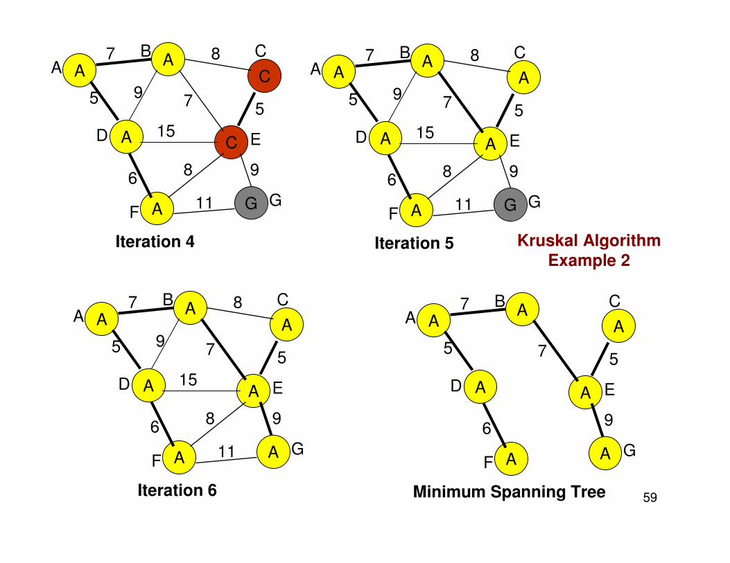
59

Kruskal Algorithm

Example 2

AA AB

C

C

AD C E

AFG G

5

7

9

8

75

15

68

11

9

Iteration 4

AA AB

A

C

AD A E

AFG G

5

7

9

8

75

15

68

11

9

Iteration 5

AA AB

A

C

AD A E

AFA G

5

7

9

8

75

15

68

11

9

Iteration 6

AA AB

A

C

AD A E

AFA G

5

7

75

69

Minimum Spanning Tree

Proof of Correctness: Kruskal’s Algorithm• Let T be the spanning tree generated by Kruskal’s algorithm for a graph

G. Let T’ be a minimum spanning tree for G. We need to show that both T and T’ have the same weight.

• Assume that wt( T’ ) < wt(T).

• Hence, there should be an edge e in T that is not in T’. Because, if every edge of T is in T’, then T = T’ and wt(T) = wt( T’ ).

• Pick up the edge e ε T and e ε T’. Include e in T’. This would create a cycle among the edges in T’. At least one edge in this cycle would not be part of T; because if all the edges in this cycle are in T, then T would have a cycle.

• Pick up the edge e’ that is in this cycle and not in T.

• Note that wt( e’ ) < wt(e); because, if this was the case then the Kruskal’s algorithm would have picked e’ ahead of e. So, wt( e’ ) ≥wt(e). This implies that we could remove e’ from the cycle and include edge e as part of T’ without increasing the weight of the spanning tree.

• We could repeat the above procedure for all edges that are in T and not in T’ ; and eventually transform T’ to T, without increasing the cost of the spanning tree.

• Hence, T is a minimum spanning tree.

61

Prim Algorithm for Min. Spanning TreeBegin Algorithm Prim (G, s)



3 End For

4 d [s] ← 0

5 S ← Φ // Optimal set of nodes that are in the minimum spanning tree

6 Q ← V // Fringe set of nodes that are not yet in the minimum spanning tree; but an estimate of an edge of the lowest weight that connects them to the tree is known.

7 While Q ≠ Φ


9 S ← S U {u}


11 If v Q and d [v] > w (u, v) then

12 d [v] ← w (u, v)


13 End If

14 End For

15 End While

16 End Prim

Note: You can select any vertex as

the starting vertex s. We are not

always guaranteed to get same

spanning tree if we start from any

vertex, but all the spanning trees will

have the same minimum weight.

∈

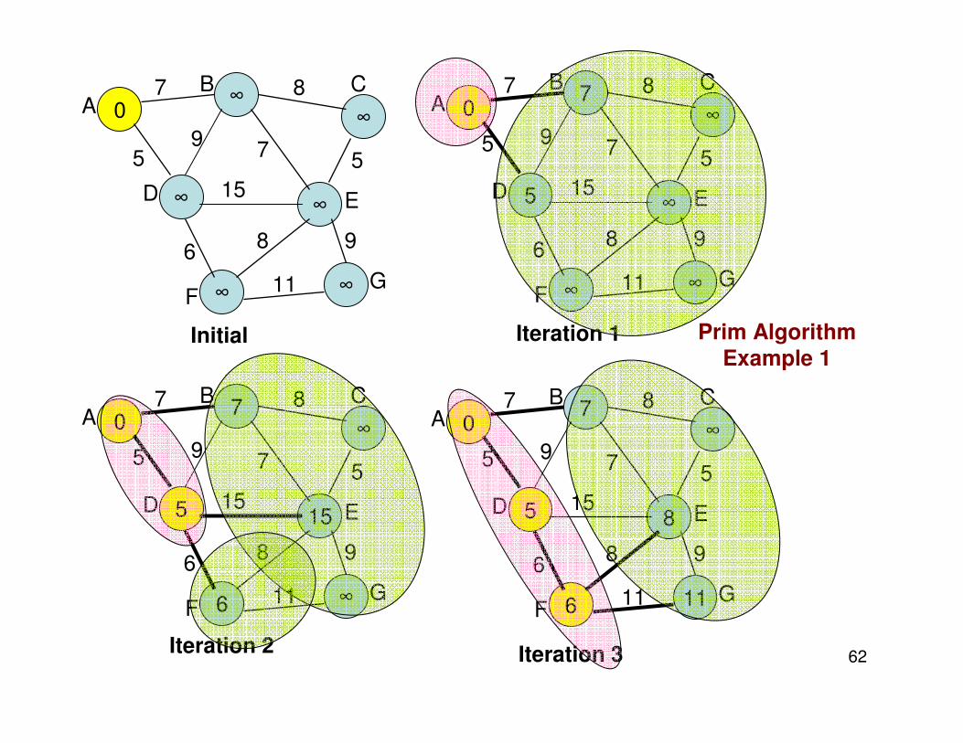
62

0A ∞B

∞

C

∞D∞ E

∞F∞ G

5

7

9

8

75

15

68

11

9

Initial

0A 7B

∞

C

5D∞ E

∞F∞ G

5

7

9

8

75

15

68

11

9

Iteration 1

0A 7B

∞

C

5D15 E

6F∞ G

5

7

9

8

75

15

68

11

9

Iteration 2

0A 7B

∞

C

5D8 E

6F11 G

5

7

9

8

75

15

68

11

9

Iteration 3

Prim Algorithm

Example 1

63

0A 7B

8

C

5D7 E

6F11 G

5

7

9

8

75

15

68

11

9

Iteration 4

0A 7B

5

C

5D7 E

6F9 G

5

7

9

8

75

15

68

11

9

Iteration 5

0A 7B

5

C

5D7 E

6F9 G

5

7

9

8

75

15

68

11

9

Iteration 6

0A 7B

5

C

5D7 E

6F9 G

5

7

9

8

75

15

68

11

9

Iteration 7

Prim Algorithm

Example 1

64

Prim Algorithm (Example 2)

∞∞0

∞∞∞

3 5

54

2

1

3

13

s

uv

wx

y

∞30

∞54

35

54

2

1

3

13

s

uv

wx

y

530

314

35

54

2

1

3

13

s

uv

wx

y

530

312

3 5

54

2

1

3

13

s

uv

wx

yv v

(a) (b) (c)

(d) (e) (f)

130

312

3 5

54

2

1

3

13

s

uv

wx

y

130

312

3 5

54

2

1

3

13

s

u

wx

y

Weight of the minimum spanning tree = 10

Weight of the shortest path tree = 12

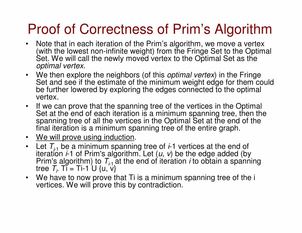
Proof of Correctness of Prim’s Algorithm• Note that in each iteration of the Prim’s algorithm, we move a vertex

(with the lowest non-infinite weight) from the Fringe Set to the Optimal Set. We will call the newly moved vertex to the Optimal Set as the optimal vertex.

• We then explore the neighbors (of this optimal vertex) in the Fringe Set and see if the estimate of the minimum weight edge for them could be further lowered by exploring the edges connected to the optimal vertex.

• If we can prove that the spanning tree of the vertices in the Optimal Set at the end of each iteration is a minimum spanning tree, then the spanning tree of all the vertices in the Optimal Set at the end of the final iteration is a minimum spanning tree of the entire graph.

• We will prove using induction.

• Let Ti-1 be a minimum spanning tree of i-1 vertices at the end of iteration i-1 of Prim's algorithm. Let (u, v) be the edge added (by Prim's algorithm) to Ti-1 at the end of iteration i to obtain a spanning tree Ti. Ti = Ti-1 U {u, v}

• We have to now prove that Ti is a minimum spanning tree of the ivertices. We will prove this by contradiction.

Proof of Correctness of Prim’s Algorithm• We assume that Ti is not a minimum spanning tree and there exists a minimum

spanning tree Ti' of these i vertices such that weight(Ti') < weight(Ti). This

implies Ti' should have been extended from a minimum spanning tree Ti-1'of

the i-1 vertices (same set of vertices spanned by Ti-1) by adding an edge (u', v')

such that at least one of the two end vertices u' and v' do not correspond to the

vertices u and v of edge (u, v) added to Ti-1 to obtain Ti; otherwise, (u', v') and

(u, v) represent the same edge and weight(Ti') = weight(Ti). Hence, for Ti' and

Ti to be of different weights, (u', v') and (u, v) should be distinct edges.

• Also, to be noted is that the vertices u' and v' should be respectively in the

Optimal Set and Fringe Set at the end of iteration i-1. Otherwise, if u' and v' are

both in the Optimal Set, then including (u', v') to Ti-1’ is only going to create a

cycle; likewise, if both u' and v' are in the Fringe Set, then Ti' is not even a

connected spanning tree.

• From the way Prim's algorithm operates, we know that edge (u, v) is the

minimal weight edge among all the edges that cross from the Optimal Set to the

Fringe Set at the end of iteration i-1. Hence, weight(u', v') ≥ weight(u, v). Since

Ti' = Ti-1' U {u', v'} and Ti = Ti-1 U {u, v}; and weight(Ti-1') = weight(Ti-1), we

can say that weight(Ti') = [ weight(Ti-1') + weight(u', v') ] ≥ [ weight(Ti-1) +

weight(u, v)] = weight(Ti). That is weight(Ti') ≥ weight(Ti). This is a

contradiction to our assumption that weight(Ti') < weight(Ti). Hence, Ti is a

minimum spanning tree at the end of iteration i of Prim's algorithm.

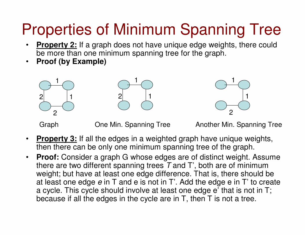
Properties of Minimum Spanning Tree• Property 2: If a graph does not have unique edge weights, there could

be more than one minimum spanning tree for the graph.• Proof (by Example)

• Property 3: If all the edges in a weighted graph have unique weights, then there can be only one minimum spanning tree of the graph.

• Proof: Consider a graph G whose edges are of distinct weight. Assume there are two different spanning trees T and T’, both are of minimum weight; but have at least one edge difference. That is, there should be at least one edge e in T and e is not in T’. Add the edge e in T’ to create a cycle. This cycle should involve at least one edge e’ that is not in T; because if all the edges in the cycle are in T, then T is not a tree.

1

2

2

1

1

2 1

1

2

1

Graph One Min. Spanning Tree Another Min. Spanning Tree

Properties of Minimum Spanning Tree• Property 3: If all the edges in a weighted graph have unique weights, then

there can be only one minimum spanning tree of the graph.

• Proof (continued..): Thus, the end vertices of each of the two edges, e and e’, should belong to two disjoint sets of vertices that if put together will be the set of vertices in the graph.

• Since all the edges in the graph are of unique weight, the weight(e’) < weight(e) for T’ to be a min. spanning tree. However, if that is the case, the weight of T can be reduced by removing e and including e’, lowering the weight of T further. This contradicts our assumption that T is a min. spanning tree.

• Hence, weight(e) weight(e’). That is, the weight of edge e cannot be greater than the weight of edge e’ for T to be a min. spanning tree. Hence, weight(e) ≤weight(e’) for T to be a min. spanning tree. Since, all edge weights are distinct, weight(e) < weight(e’) for T to be a min. spanning tree.

• However, from the previous argument, we have that weight(e’) < weight(e) for T’ to be a min. spanning tree.

• Thus, even though the graph has unique edge weights, it is not possible to say which of the two edges (e and e’) are of greater weight, if the graph has two minimum spanning trees.

• Thus, a graph with unique edge weights has to have only one minimum spanning tree.

T T’

e’

e

T Modified T’

e’

e e

W(e) < W(e’) => T’ is not a MST

W(e) > W(e’) => T is not a MST

Hence, for both T and T’ to be different MSTs � W(e) = W(e’).

But the graph has unique edge weights.

W(e) ≠W(e) � Both T and T’ have to be the same.

Assume that both T and T’ are MSTs, but different MSTs to start with.

Property 3

Maximum Spanning Tree• A Maximum Spanning Tree is a spanning tree such that

the sum of its edge weights is the maximum.

• We can find a Maximum Spanning Tree through any one of the following ways:– Run Kruskal’s algorithm by selecting edges in the decreasing

order of edge weights (i.e., edge with the largest weight is chosen first) as long as the end vertices of an edge are in two different components

– Run Prim’s algorithm by selecting the edge with the largest weight crossing from the optimal set to the fringe set

– Given a weighted graph, set all the edge weights to be negative,run a minimum spanning tree algorithm on the negative weight graph, then turn all the edge weights to positive on the minimumspanning tree to get a maximum spanning tree.

71

AA BB

C

C

DDE E

FFG G

5

7

9

8

75

15

68

11

9

Initial Kruskal Algorithm

Example 2 for

Max. Spanning Tree

Iteration 1

Iteration 2 Iteration 3

AA BB

C

C

DDE E

FFG G

5

7

9

8

75

15

68

11

9

AA BB

C

C

DDE E

FFG G

5

7

9

8

75

15

68

11

9

AA BB

C

C

DDE E

FFG G

5

7

9

8

75

15

68

11

9

72

Iteration 4 Iteration 5

Iteration 6 Maximum Spanning Tree

AA BB

C

C

DDE E

FFG G

5

7

9

8

75

15

68

11

9

AA BB

C

C

DDE E

FFG G

5

7

9

8

75

15

68

11

9

AA BB

C

C

DDE E

FFG G

5

7

9

8

75

15

68

11

9

AA BB

C

C

DDE E

FFG G

7

9

8

15

11

9

5.5 All Pairs Shortest Paths Problem

Floyd’s Algorithm: All pairs

shortest paths

Problem: In a weighted (di)graph, find shortest paths between

every pair of vertices

idea: construct solution through series of matrices D(0), …,

D (n) using increasing subsets of the vertices allowed

as intermediate

Example: 3

42

1

4

1

61

5

3

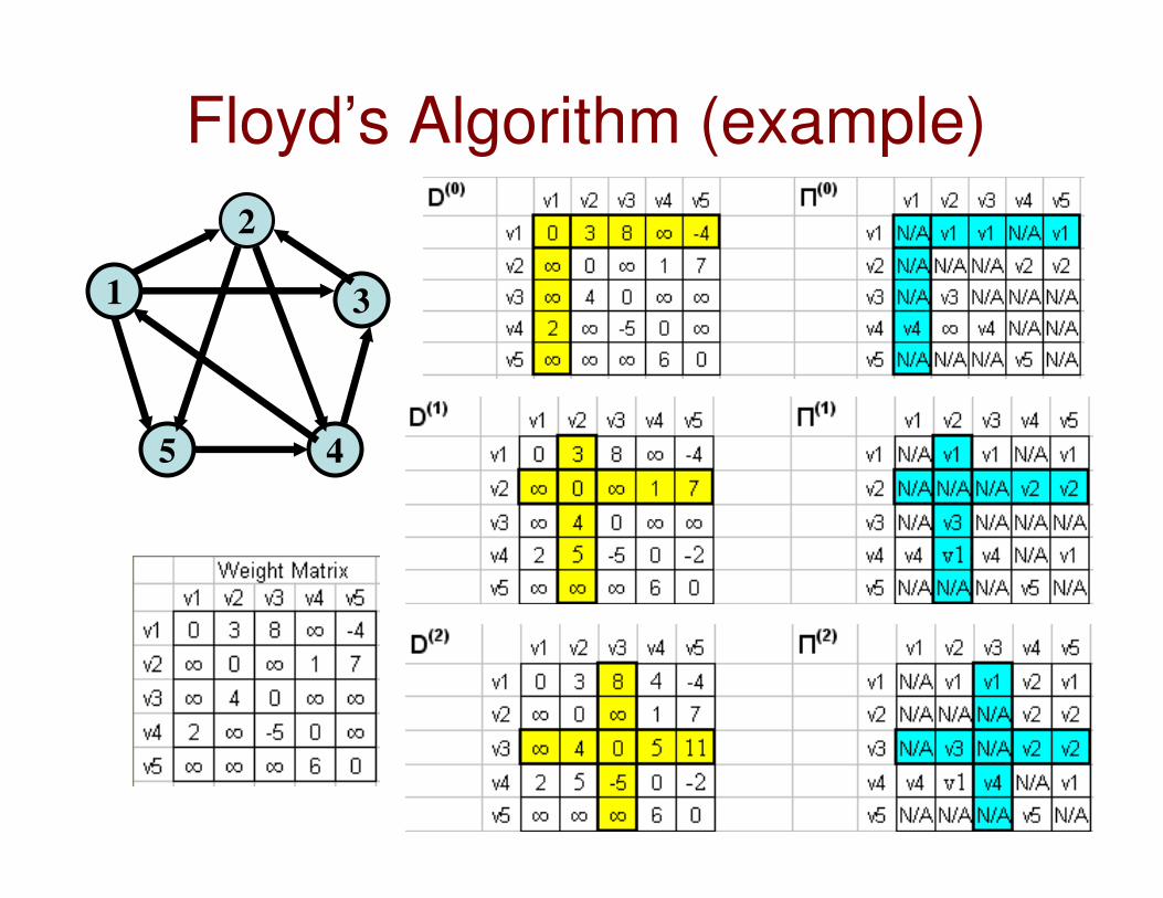
Floyd’s Algorithm

(matrix generation)On the k-th iteration, the algorithm determines shortest paths

between every pair of vertices i, j that use only vertices among

1,…,k as intermediate

D(k)[i,j] = min {D(k-1)[i,j], D(k-1)[i,k] + D(k-1)[k,j]}

i

j

k

D(k-1)[i,j]

D(k-1)[i,k]

D(k-1)[k,j]

Predecessor Matrix

Floyd’s Algorithm (example)

31

3

2

6 7

4

1 2


31

3

2

6 7

4

1 2

31

3

2

6 7

4

1 2

Floyd’s Algorithm (pseudocode and analysis)

Time efficiency: Θ(n3)

Space efficiency: Θ(n2)


1 3

45

2


Deducing path from v1 to v3

Module 5 Graph Algorithms - Jackson State University

Documents

Transcript of Module 5 Graph Algorithms - Jackson State University