
MODULE 3: CASE STUDIES Professor D.N.P. Murthy The University of Queensland Brisbane, Australia.
45
MODULE 3: CASE STUDIES MODULE 3: CASE STUDIES Professor D.N.P. Murthy Professor D.N.P. Murthy The University of The University of Queensland Queensland Brisbane, Australia Brisbane, Australia
-
Upload
roberta-sanders -
Category
Documents
-
view
230 -
download
2
Transcript of MODULE 3: CASE STUDIES Professor D.N.P. Murthy The University of Queensland Brisbane, Australia.

MODULE 3: CASE STUDIESMODULE 3: CASE STUDIES
Professor D.N.P. MurthyProfessor D.N.P. Murthy
The University of QueenslandThe University of Queensland
Brisbane, AustraliaBrisbane, Australia

CASE STUDY - 1CASE STUDY - 1
Source: Source: Warranty Cost Analysis Warranty Cost Analysis
[Chapter 13][Chapter 13]
Item: Item: Aircraft componentAircraft component
Problem:Problem: Item supplied without warrantyItem supplied without warranty Customer requests two-year warrantyCustomer requests two-year warranty Select warranty termsSelect warranty terms Predict costsPredict costs

Data and AnalysisData and Analysis
Operational dataOperational data88 failure times 88 failure times
65 service times65 service times
Repairable item: Repaired back to newRepairable item: Repaired back to new Special analysis required Special analysis required
((“incomplete data”)“incomplete data”)
Weibull distribution fits the data Weibull distribution fits the data (Increasing failure rate: Shape parameter > 1)(Increasing failure rate: Shape parameter > 1)
Data and Analysis [Cont.]Data and Analysis [Cont.]
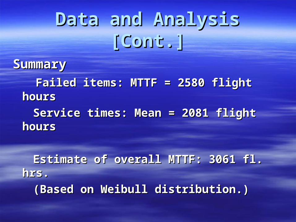
SummarySummary
Failed items: MTTF = 2580 flight hoursFailed items: MTTF = 2580 flight hours
Service times: Mean = 2081 flight hoursService times: Mean = 2081 flight hours
Estimate of overall MTTF: 3061 fl. hrs.Estimate of overall MTTF: 3061 fl. hrs.
(Based on Weibull distribution.)(Based on Weibull distribution.)

Policies ConsideredPolicies Considered
1. Nonrenewing FRW, W = 5000 fl. hrs.1. Nonrenewing FRW, W = 5000 fl. hrs.
2. Nonrenewing FRW, W = 2 years, 2. Nonrenewing FRW, W = 2 years, calendar time calendar time
3. Rebate PRW, W = 50003. Rebate PRW, W = 5000
4. Rebate PRW, W = 2 years4. Rebate PRW, W = 2 years
(Average usage rate: 3061 flight hours per (Average usage rate: 3061 flight hours per year)year)

ResultsResults
Costs: cs = $9000 cb = $17500 cr = $5400 Costs: cs = $9000 cb = $17500 cr = $5400
Policy Estimated CostPolicy Estimated Cost
11 $15,669$15,669
22 18,978 18,978
33 13,300 13,300
44 16,098 16,098

CASE STUDY - 2CASE STUDY - 2
Product: Microwave LinksProduct: Microwave LinksMajor componentsMajor components
Crystal ReceiverCrystal Receiver Crystal Transmitter Crystal Transmitter 2Mb card 2Mb card 2Mb PCM card 2Mb PCM card

CASE STUDY - 2CASE STUDY - 2 Sold in lots (size varying from 1 - 100)Sold in lots (size varying from 1 - 100) Sold with 3 year FRW policySold with 3 year FRW policy Failed items returned in batchesFailed items returned in batches No information about No information about
– the time at which the item was put in usethe time at which the item was put in use– the time at which the item failedthe time at which the item failed

Manufacturing Cost Data
Customer
Order
Number
Number
of Systems
in Batch
Labour
Cost
($)
Material
Cost
($)
Overhead
Recovered
($)
Direct
Expenses
($)
Total
Cost
($)
Average
Cost per
System ($)
034-1605 2 1329 11474 929 0 13732 6866.00
034-1616 24 18155 131811 12355 1035 163356 6806.50
034-1758 2 2665 11940 1865 0 16470 8235.00
034-1809 38 30600 178243 21415 0 230258 6059.42
034-1899 2 1800 10250 1260 0 13310 6655.00
056-1976 4 2812 29448 1966 0 34226 8556.50
068-1838 4 3966 27528 2776 0 34270 8567.50
072-1955 2 1238 18782 867 0 20887 10443.50
099-1429 100 72900 529900 51100 7100 661000 6610.00
106-1682 16 14180 132379 9928 1386 157873 9867.06
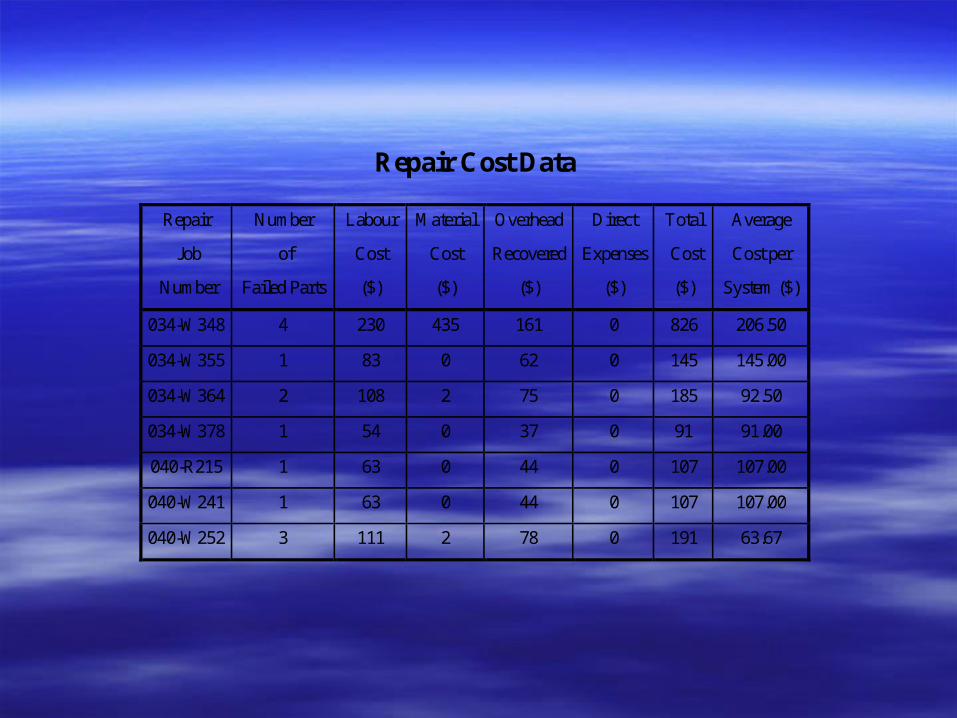
Repair Cost Data
Repair
Job
Number
Number
of
Failed Parts
Labour
Cost
($)
Material
Cost
($)
Overhead
Recovered
($)
Direct
Expenses
($)
Total
Cost
($)
Average
Cost per
System ($)
034-W348 4 230 435 161 0 826 206.50
034-W355 1 83 0 62 0 145 145.00
034-W364 2 108 2 75 0 185 92.50
034-W378 1 54 0 37 0 91 91.00
040-R215 1 63 0 44 0 107 107.00
040-W241 1 63 0 44 0 107 107.00
040-W252 3 111 2 78 0 191 63.67
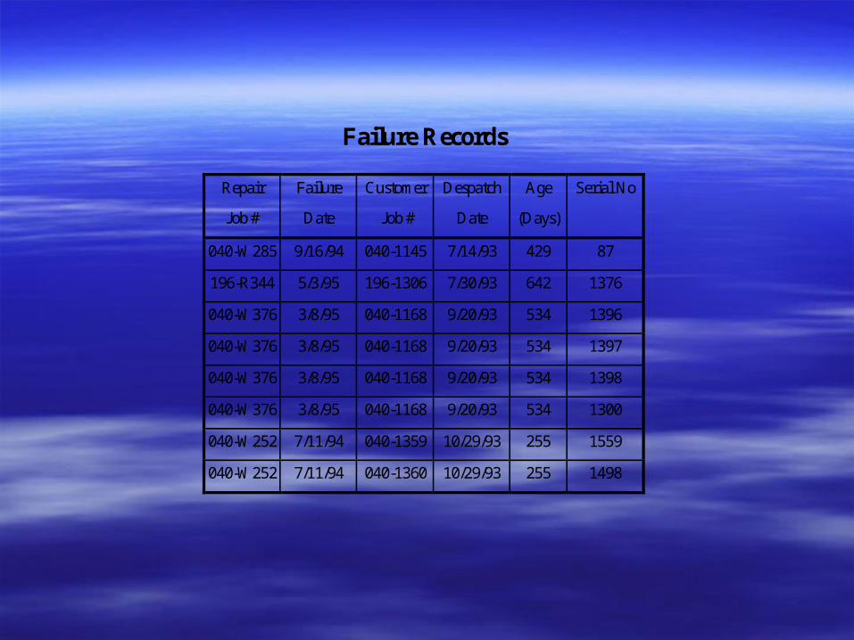
Failure Records
Repair
Job #
Failure
Date
Customer
Job #
Despatch
Date
Age
(Days)
Serial No
040-W285 9/16/94 040-1145 7/14/93 429 87
196-R344 5/3/95 196-1306 7/30/93 642 1376
040-W376 3/8/95 040-1168 9/20/93 534 1396
040-W376 3/8/95 040-1168 9/20/93 534 1397
040-W376 3/8/95 040-1168 9/20/93 534 1398
040-W376 3/8/95 040-1168 9/20/93 534 1300
040-W252 7/11/94 040-1359 10/29/93 255 1559
040-W252 7/11/94 040-1360 10/29/93 255 1498

Survival Records
Customer
Job
Number
Despatch
Date
Number
of
Systems
Date of
Data
Collection
Age (Days) at
Date of Data
Collection
196-1306 7/30/93 2 6/9/95 679
196-1322 9/11/93 2 6/9/95 636
355-1336 9/24/93 2 6/9/95 623
040-1358 10/29/93 2 6/9/95 588
040-1359 10/29/93 2 6/9/95 588
040-1360 10/29/93 2 6/9/95 588
040-1361 10/29/93 2 6/9/95 588
034-1393 11/12/93 10 6/9/95 574

Data used in MATLAB program for analysis
Batch
Number
j
Batch
Size
Nj
Age of
Batch
Tj
Number of
Failures in Batch
nj
Failure
Times
xji
1 2 679 1 642
2 2 636 0
3 2 623 0
4 2 588 0
5 2 588 2 255
350
6 2 588 3 255
354

ESTIMATES BASED ON ESTIMATES BASED ON DATA ANALYSISDATA ANALYSIS
Manufacturing Cost per Item, Cs = Manufacturing Cost per Item, Cs = $7316.18$7316.18
Repair Cost per Item, Cr = $143.94Repair Cost per Item, Cr = $143.94 Weibull scale parameter, Weibull scale parameter, = 0.43233 = 0.43233 Weibull shape parameter, Weibull shape parameter, = 1.57479 = 1.57479

0.00
0.20
0.40
0.60
0.80
1.00
1.20
1.40
0 1 2 3 4 5 6 7
Time (Years)
Fai
lure
Rat
e r(
t)

0
0.05
0.1
0.15
0.2
0.25
0.3
0.35
0 1 2 3 4 5 6 7
Time (Years)
f(t)
0.00
50.00
100.00
150.00
200.00
250.00
300.00
350.00
400.00
0 5 10 15 20 25
Number of Items
Rep
air
Co
st p
er I
tem
($)
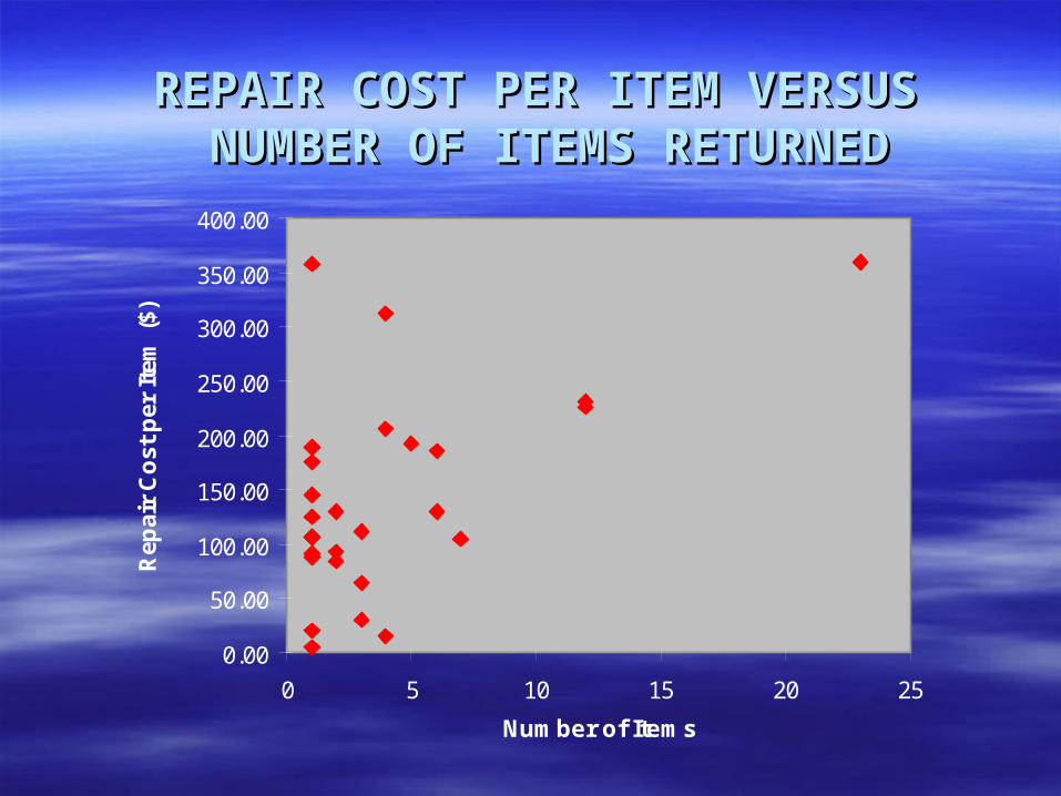
REPAIR COST PER ITEM VERSUS REPAIR COST PER ITEM VERSUS NUMBER OF ITEMS RETURNEDNUMBER OF ITEMS RETURNED

WARRANTY SERVICING COST FOR WARRANTY SERVICING COST FOR DIFFERENT WARRANTY PERIODSDIFFERENT WARRANTY PERIODS..
Warranty
Period
(Years)
W
Expected
Number of Failures
in Warranty Period
M(W)
Warranty
Servicing
Cost ($)
cr*M(W)
Warranty Servicing Cost
as a percentage of
the manufacture cost
1 0.27 38.43 0.53
2 0.80 114.48 1.56
3 1.51 216.78 2.96
4 2.37 341.02 4.66
5 3.37 484.61 6.62
6 4.49 645.78 8.83
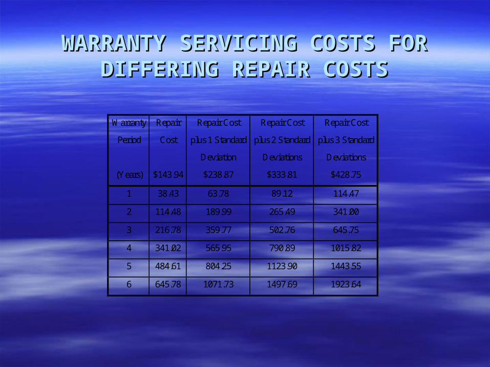
WARRANTY SERVICING COSTS FOR WARRANTY SERVICING COSTS FOR DIFFERING REPAIR COSTSDIFFERING REPAIR COSTS
Warranty
Period
(Years)
Repair
Cost
$143.94
Repair Cost
plus 1 Standard
Deviation
$238.87
Repair Cost
plus 2 Standard
Deviations
$333.81
Repair Cost
plus 3 Standard
Deviations
$428.75
1 38.43 63.78 89.12 114.47
2 114.48 189.99 265.49 341.00
3 216.78 359.77 502.76 645.75
4 341.02 565.95 790.89 1015.82
5 484.61 804.25 1123.90 1443.55
6 645.78 1071.73 1497.69 1923.64

WARRANTY SERVICING COSTS FOR WARRANTY SERVICING COSTS FOR VARYING SCALE PARAMETERVARYING SCALE PARAMETER
Warranty
Period
(Years)
99.9%
Confidence
Interval for
Lower Limit
0.42295
99%
Confidence
Interval for
Lower Limit
0.42499
95%
Confidence
Interval for
Lower Limit
0.42674
Point
Estimate
for
0.43233
95%
Confidence
Interval for
Upper Limit
0.43793
99%
Confidence
Interval for
Upper Limit
0.43968
99.9%
Confidence
Interval for
Upper Limit
0.44172
1 37.12 37.41 37.65 38.43 39.21 39.46 39.75
2 110.59 111.43 112.15 114.48 116.82 117.56 118.42
3 209.42 211.01 212.38 216.78 221.21 222.61 224.24
4 329.43 331.93 334.10 341.02 347.99 350.19 352.75
5 468.14 471.70 474.77 484.61 494.52 497.64 501.28
6 623.84 628.58 632.68 645.78 658.98 663.15 668.00

WARRANTY SERVICING COSTS FOR WARRANTY SERVICING COSTS FOR VARYING SHAPE PARAMETER VARYING SHAPE PARAMETER
Warranty
Period
(Years)
99.9%
Confidence
Interval for
Lower Limit
1.56540
99%
Confidence
Interval for
Lower Limit
1.56744
95%
Confidence
Interval for
Lower Limit
1.56920
Point
Estimate
for
1.57479
95%
Confidence
Interval for
Upper Limit
1.58038
99%
Confidence
Interval for
Upper Limit
1.58214
99.9%
Confidence
Interval for
Upper Limit
1.58418
1 38.73 38.67 38.61 38.43 38.25 38.19 38.13
2 114.63 114.60 114.57 114.48 114.38 114.35 114.32
3 216.25 216.37 216.47 216.78 217.10 217.20 217.31
4 339.27 339.65 339.98 341.02 342.06 342.39 342.78
5 481.11 481.87 482.52 484.61 486.70 487.36 488.13
6 640.03 641.27 642.35 645.78 649.23 650.32 651.58

CASE STUDY: CASE STUDY: PHOTOCOPIERPHOTOCOPIER
[Service Agent Perspective][Service Agent Perspective]

DATA FOR MODELLINGDATA FOR MODELLING
Supplied by the Supplied by the service agent service agent
Single machine: Single machine: Failures over a 5 year Failures over a 5 year periodperiod
Part of the data is Part of the data is shown on the left shown on the left sideside
Count Day Component 60152 29 Cleaning Web 60152 29 Toner Filter 60152 29 Feed Rollers
132079 128 Cleaning Web 132079 128 Drum Cleaning Blade 132079 128 Toner Guide 220832 227 Toner Filter 220832 227 Cleaning Blade 220832 227 Dust Filter 220832 227 Drum Claws 252491 276 Drum Cleaning Blade 252491 276 Cleaning Blade 252491 276 Drum 252491 276 Toner Guide 365075 397 Cleaning Web 365075 397 Toner Filter

MODELLINGMODELLING
One can either use number of copies One can either use number of copies (count) or time (age) as the variable in (count) or time (age) as the variable in modelling at both component and modelling at both component and system levelsystem level
The count and time between failures are The count and time between failures are correlated (correlation coefficient 0.753)correlated (correlation coefficient 0.753)

COMPONENT FAILURESCOMPONENT FAILURES
Photocopier has Photocopier has several componentsseveral components
Frequency Frequency distribution of distribution of component failures component failures is given on the left is given on the left
Failed Component Frequency Cleaning web 15 Toner filter 6 Feed rollers 11 Drum blade 2 Toner guide 7 Cleaning blade 7 Dust filter 6 Drum claws 5 Crum 6 Ozone filter 8 Upper fuser roller 5 Upper roller claws 5 TS block front 2 Charging wire 6 Lower roller 2 Optics PS felt 3 Drive gear D 2
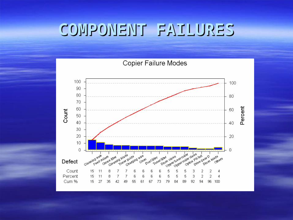
COMPONENT FAILURESCOMPONENT FAILURES

SYSTEMSYSTEM LEVEL MODELLINGLEVEL MODELLING

SERVICE CALLSSERVICE CALLS
Service calls modelled as a point Service calls modelled as a point process through rate of occurrence process through rate of occurrence of failure (ROCOF) which defines of failure (ROCOF) which defines probability of service call in a short probability of service call in a short interval as a function of age (time)interval as a function of age (time)
ROCOF: Weibull intensity function ROCOF: Weibull intensity function : Scale parameter : Scale parameter : Shape parameter: Shape parameter
( 1)( ) ( / )t t

SERVICE CALLSSERVICE CALLS
The shape parameter The shape parameter > 1 implies that > 1 implies that service call frequency increases (due to service call frequency increases (due to reliability decreasing) with time (age) reliability decreasing) with time (age)
Data indicates that this is indeed the Data indicates that this is indeed the case. The next slide verifies this where case. The next slide verifies this where TTF denotes the time between service TTF denotes the time between service calls. calls.

Actual
Fits
Actual
Fits
403020100
100
50
0
TT
F-S
yste
m
Time
Yt = 75.6950 - 1.70911*t
MSD:MAD:MAPE:
344.096 14.479 44.989
Trend Analysis for TTF-SystemLinear Trend Model
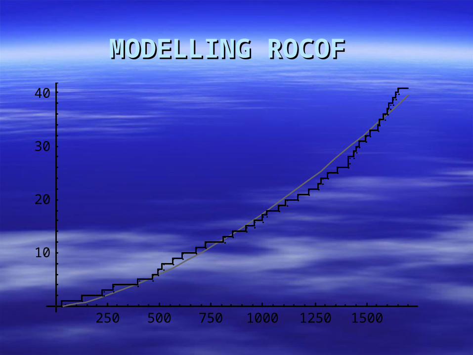
MODELLING ROCOFMODELLING ROCOF
250 500 750 1000 1250 1500
10
20
30
40

MODELLING ROCOFMODELLING ROCOF
Time used as the variable in the Time used as the variable in the modellingmodelling
= 157.5 days, = 157.5 days, = 1.55 = 1.55 Estimated average number of service Estimated average number of service
calls per year: calls per year:
Year
Estimated Service Calls 3.7 7.1 9.4 11.3 13.0 14.6 16.0 17.3 18.5 19.7
1.

COMPONENT LEVEL MODELLINGCOMPONENT LEVEL MODELLING
COMPONENT: CLEANING WEBCOMPONENT: CLEANING WEB

MODELLINGMODELLING
Failed components replaced by new Failed components replaced by new onesones
Time to failure modelled by a failure Time to failure modelled by a failure distribution function distribution function FF(t)(t)
The form of the distribution function The form of the distribution function determined using the failure data determined using the failure data available (black-box modelling)available (black-box modelling)

MODELLINGMODELLING
Several distribution function were Several distribution function were examined for modelling at the examined for modelling at the component level. Some of them were: component level. Some of them were:
2- and 3-parameter (delayed) Weibull2- and 3-parameter (delayed) Weibull Mixture WeibullMixture Weibull Competing risk WeibullCompeting risk Weibull Multiplicative WeibullMultiplicative Weibull Sectional WeibullSectional Weibull

COMPONENT LEVELCOMPONENT LEVEL
A list of the different distributions A list of the different distributions considered can in found in the following considered can in found in the following book: Murthy, D.N.P., Xie, M. and Jiang, book: Murthy, D.N.P., Xie, M. and Jiang, R. (2003), R. (2003), Weibull ModelsWeibull Models, Wiley, New , Wiley, New YorkYork
We consider modelling based on both We consider modelling based on both “counts” and “age” “counts” and “age”

HISTOGRAM (COUNTS)HISTOGRAM (COUNTS)
24000020000016000012000080000400000
5
4
3
2
1
0
cleaning web counter
Fre
que
ncy
Cleaning W eb Counter
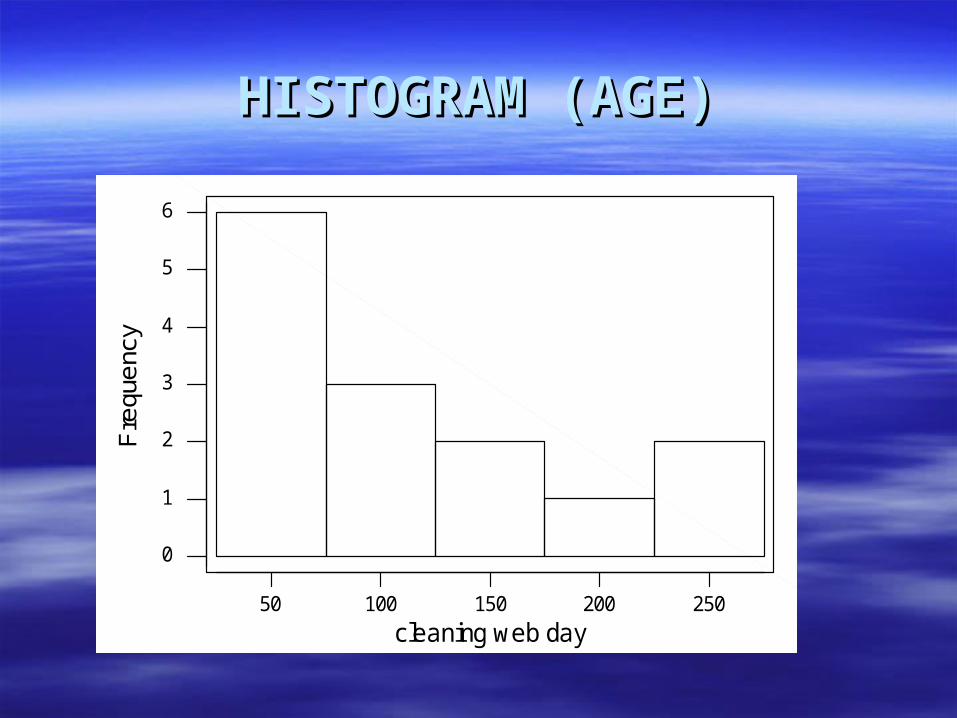
HISTOGRAM (AGE)HISTOGRAM (AGE)
25020015010050
6
5
4
3
2
1
0
cleaning web day
Fre
que
ncy
Cleaning Web Day

WPP PLOTWPP PLOT
WPP plot allows one to decide if one of WPP plot allows one to decide if one of the Weibull models is appropriate for the Weibull models is appropriate for modelling a given data setmodelling a given data set
For 2-parameter Weibull: WPP is a For 2-parameter Weibull: WPP is a straight linestraight line
For more on WPP plot, see For more on WPP plot, see Weibull Weibull Models Models by Murthy et al (cited earlier)by Murthy et al (cited earlier)

NOTATIONNOTATION
Two sub-populationsTwo sub-populations Scale parametersScale parameters Shape parameters Shape parameters Location parameter Location parameter Mixing parameter Mixing parameter pp error: error: (square of the error between model (square of the error between model
and data on the WPP)and data on the WPP)
1 2, 1 2,
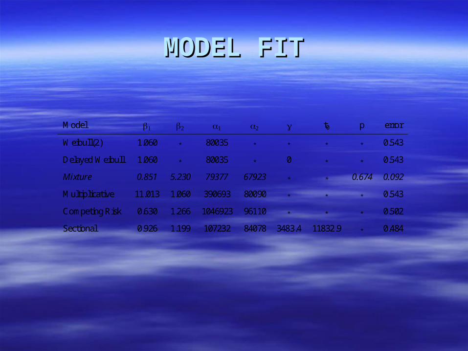
MODEL FITMODEL FIT
Model t0 p error
Weibull(2) 1.060 * 80035 * * * * 0.543
Delayed Weibull 1.060 * 80035 * 0 * * 0.543
Mixture 0.851 5.230 79377 67923 * * 0.674 0.092
Multiplicative 11.013 1.060 390693 80090 * * * 0.543
Competing Risk 0.630 1.266 1046923 96110 * * * 0.502
Sectional 0.926 1.199 107232 84078 3483.4 11832.9 * 0.484

MIXTURE MODEL (COUNT)MIXTURE MODEL (COUNT)

SPARES NEEDEDSPARES NEEDED
The average number of spares needed The average number of spares needed each year can be obtained by solving the each year can be obtained by solving the renewal integral equation. See, the book renewal integral equation. See, the book on on Reliability Reliability by Blischke and Murthy by Blischke and Murthy (cited earlier) for details. It is as follows:(cited earlier) for details. It is as follows:
Year
Estimated Cleaning Webs 2.83 3.04 3.04 3.04 3.04 3.04 3.04 3.04 3.04 3.04
REFERENCEREFERENCE
For further details of this case study, For further details of this case study, see, Bulmer M. and Eccleston J.E. see, Bulmer M. and Eccleston J.E. (1992), Photocopier Reliability Modeling (1992), Photocopier Reliability Modeling Using Evolutionary Algorithms, Chapter Using Evolutionary Algorithms, Chapter 18 in Case Studies in 18 in Case Studies in Reliability and Reliability and MaintenanceMaintenance , , Blischke, W.R. and Murthy, Blischke, W.R. and Murthy, D.N.P. (eds) (1992), Wiley, New York D.N.P. (eds) (1992), Wiley, New York

Thank youThank you