Module 19

Region of Convergence (ROC)

(Z-Transforms)

Objective : To understand the meaning of ROC in Z transforms and the need to consider it.

Introduction :

As we are aware that the Z- transform of a discrete signal x(n) is given by

𝑋 𝑧 = 𝑥 𝑛 𝑧−𝑛∞

𝑛=−∞

The Z-transform has two parts which are, the expression and Region of Convergence

respectively.

Whether the Z-transform X(z) of a signal x(n) exists or not depends on the complex

variable „z‟ as well as the signal itself. All complex values of „z=rejω

‟ for which the

summation in the definition converges form a region of convergence (ROC) in the z-plane. A

circle with r=1 is called unit circle and the complex variable in z-plane is represented as

shown below.

Description :

The concept of ROC can be understood easily by finding z transform of two functions given

below:

a) 𝑥 𝑛 = 𝑎𝑛𝑢(𝑛)

𝑋 𝑧 = 𝑎𝑛𝑢(𝑛)𝑧−𝑛∞

𝑛=−∞

= 𝑎𝑛𝑧−𝑛 = 𝑎𝑧−1 𝑛∞

𝑛=0

∞

𝑛=0

For convergence of X(z), we require that 𝑎𝑧−1 𝑛∞𝑛=0 < ∞. Consequently, the

region of convergence is that range of values of z for which 𝑎𝑧−1 < 1, or

equivalently, 𝑧 > 𝑎 and is shown in figure below

Then 𝑋 𝑧 = 𝑎𝑧−1 𝑛∞𝑛=0 =

1

1−𝑎𝑧−1 =𝑧

𝑧−𝑎

b) 𝑥 𝑛 = −𝑎𝑛𝑢(−𝑛 − 1)

𝑋 𝑧 = −𝑎𝑛𝑢(−𝑛 − 1) 𝑧−𝑛∞

𝑛=−∞

= − 𝑎𝑛𝑧−𝑛 = − 𝑎−1𝑧 𝑛∞

𝑛=1

−1

𝑛=−∞

= 1 − 𝑎−1𝑧 𝑛∞

𝑛=0

= 1 −1

1 − 𝑎−1𝑧=

1

1 − 𝑎𝑧−1=

𝑧

𝑧 − 𝑎

This result converges only when 𝑎−1𝑧 < 1, or equivalently, |z| < |a|. The ROC is shown

below

Need to consider region of convergence while determining the z-transform

If we consider the signals anu(n) and -a

nu(-n-1), we note that although the signals are

differing, their z Transforms are identical which is 𝑧

𝑧−𝑎. Thus we conclude that to distinguish

zTransforms uniquely their ROC's must be specified.

Zeros and Poles of the Laplace Transform

LikeLaplace transforms as studied earlier in Module-15, the z-transforms in the above

examples are rational, i.e., they can be written as a ratio of polynomials of variable „z‟in the

general form

𝑋 𝑧 =𝑁(𝑧)

𝐷 𝑧 =

𝑏𝑘𝑧−𝑘𝑀

𝑘=0

𝑎𝑘𝑧−𝑘𝑁

𝑘=0

= 𝑧−𝑧𝑧𝑘

𝑀𝑘=1

𝑧−𝑧𝑝𝑘𝑁𝑘=1

.

N(z) is the numerator polynomial of order M withzzk,(k=1,2,…,M) roots

D(z) is the denominator polynomial of order N with zpk(k=1,2,…,N) roots

Roots of numerator polynomial are called zeros and the roots of denominator polynomial are

called poles. Poles in z-plane are indicated with „x‟ and zeros with‟o‟ similar to s-plane. The

representation of X(z) through its poles and zeros in the z-plane is referred to as the pole-zero

plot of X(z).

In general, we assume the order of the numerator polynomial is always lower than that of the

denominator polynomial, i.e., M<N. If this is not the case, we can always expand X(z) into

multiple terms so that M<N is true for each of terms.

Properties of ROC:

In Module-15 we saw that there were specific properties of the region of convergence of the

Laplace transform for different classes of signals and that understanding these properties led

to further insights about the transform. In a similar manner, we explore a number of

properties of the region of convergence for the z-transform

Property 1:The ROC of X(z) consists of a ring in the z-plane centered about the origin.

This property is illustrated in figure below and follows from the fact that the ROC

consists of those values of z=rejω

for which x(n)r-n

has a Fourier transform that converges.

That is, the ROC of the z-transform of x(n) consists of the values of z for which x(n)r-n

is

absolutely summable.

𝑥(𝑛) 𝑟−𝑛 < ∞

∞

𝑛=−∞

Thus, convergence is dependent only on r=|z| and not on ω. Consequently, if a

specific value of z is in the ROC, then all values of z on the same circle (i.e., with the same

magnitude) will be in ROC. This by itself guarantees that ROC will consist of concentric

rings.

In some cases, the inner boundary of the ROC may extend inward to the origin, and in

some cases the outer boundary may extend outward to infinity.

Property 2:If the z-transform X(z) of x(n) is rational, then the ROC does not contain any

poles but is bounded by poles or extend to infinity.

As with the Laplace transform, this property is simply a consequence of the fact that

at a pole X(z) is infinite and therefore does not converge.

Property 3: If x(n) is of finite duration, then the ROC is the entire z-plane, except possibly

z=0 and / or z=∞

A finite duration sequence has only a finite number of nonzero values, extending, say,

from n=N to n=M, where N and M are finite. Thus the z-transform is the sum of a finite

number of terms; that is

𝑋 𝑧 = 𝑥 𝑛 𝑧−𝑛𝑀

𝑛=𝑁

For z not equal to zero or infinity, each term in the sum will be finite, and

consequently X(z) will converge.

If N is negative and M is positive, so that x(n) has nonzero values both for n<0 and

n>0, then the summation includes terms with both positive and negative powers of z. As

|z|→0, terms involving negative powers of z, become unbounded, and as |z|→∞, terms

involving positive powers of z become unbounded. Consequently, for N negative and M

positive, the ROC does not include z=0 or z=∞.

If N is zero or positive, there are only negative powers of z and consequently, the

ROC includes z=∞. If M is zero or negative, there are only positive powers of z and

consequently, the ROC includes z=0.

Illustration

Consider the unit impulse signal 𝛿 𝑛 . Its z-transform is given by

𝛿(𝑛)Ζ 𝛿 𝑛 𝑧−𝑛 = 1

∞

𝑛=−∞

with an ROC consisting of the entire z-plane, including z=0 and z=∞. On the other hand,

consider the delayed unit impulse 𝛿 𝑛 − 1 , for which

𝛿(𝑛 − 1)Ζ 𝛿 𝑛 − 1 𝑧−𝑛 = 𝑧−1

∞

𝑛=−∞

This z-transform is well defined except at z=0 where there is a pole. Thus, the ROC consists

of the entire z-plane, including z=∞ but excluding z=0. Similarly, consider an impulse

advanced in time by one unit, namely 𝛿 𝑛 + 1 .

𝛿(𝑛 + 1)Ζ 𝛿(𝑛 + 1)𝑧−𝑛 = 𝑧

∞

𝑛=−∞

In this case, ROC consists of the entire finite z-plane (including z=0), but there is

a pole at infinity.

Property 4: If x(nt) is a right sided sequence, and if the circle |z|=ro is in the ROC, then all

finite values of z for which |z|>ro will also be in the ROC.

The justification for this property follow in a manner identical to that in Laplace

transforms. A right sided sequence is zero prior to some value of n, say N1. If the circle |z|=ro

is in the ROC, then x(n)r-n

is absolutely summable. Now consider |z| =r1 with r1>ro, so that r1-n

decays quickly than ro-n

for increasing n as illustrated in the figure below.

Consequently, x(n)r1-n

is absolutely summable.

For right sided sequences in general 𝑋 𝑧 = 𝑥 𝑛 𝑧−𝑛∞𝑛=𝑁1 , where N1 is finite and may be

positive or negative.

If N1 is negative, then the summation above includes terms with positive powers of z, which

become unbounded as |z|→∞. Consequently, for right sided sequences in general, ROC will

not include infinity.

However, for causal sequences, i.e., sequences that are zero for n<0, N1 will be non-negative,

and consequently, the ROC will include z=∞

Property 5: If x(n) is a left sided sequence, and if the circle|z|=ro is in the ROC, then all

values of z for which 0<|z|<ro will also be in the ROC.

For left sided sequences, the summation for the z-transform will be of the form

𝑥 𝑧 = 𝑥 𝑛 𝑧−𝑛𝑀

𝑛=−∞

where M may be positive or negative. If M is positive, then the transform includes

negative powers of z, which become unbounded as |z|→0. Consequently, for left-sided

sequences, the ROC will not include |z|=0. However, if M≤0 (so that x(n)=0 for all n>0), the

ROC will include z=0.

Property 6: If x(n) is two sided, and if the circle |z|=ro is in the ROC, then the ROC will

consist of a ring in the z-plane that includes the circle |z|=ro.

Like corresponding property in Laplace transforms, the ROC of a two-sided signal

can be examined by expressing x(n) as the sum of a right-sided and a left-sided signal. The

ROC for the right-sided component is a region bounded on the inside by a circle and

extending outward to (and possibly including) infinity as in figure (a). The ROC for the left-

sided component is a region bounded on the outside by a circle and extending inward to, and

possibly including, the origin as in figure (b). The ROC for the composite signal includes the

intersection of the ROCs of the components as in figure (c).

Property 7: Ifthe z-transform X(z) of x(n) is rational, and if x(n) is right sided, then the ROC

is the region in the z-plane outside the outermost pole i.e., outside the circle of radius equal

to the largest magnitude of the poles of X(z).

Property 8:If the z-transform X(z) of x(n) is rational, and if x(n) is left sided, then the ROC is

the region in the z-plane inside the innermost pole i.e., inside the circle of radius equal to the

smallest magnitude of the poles of X(z) other than any at z=0 and extending inward to and

possibly including z=0.

Analysis and characterization of Discrete Time LTI systems using z- transform:

One of the important applications of the z-transform is in the analysis and

characterization of Discrete Time LTI systems.

Causality: For a causal LTI system, the impulse response is zero for n<0 and thus is right

sided.

A discrete time LTI system with rational system function H(z) is causal if and only if :

(i) The ROC is the exterior of a circle outside the outermost pole

(ii) With H(z) expressed as a ratio of polynomials in z, the order of the numerator

cannot be greater than the order of the denominator

Stability:The stability of a Discrete time LTI system is equivalent to its impulse response

being absolutely summable.

(i) An LTI system is stable if and only if the ROC of its system function H(z)

includes the unit circle [i.e., |z|=1]

(ii) A causal LTI system with rational transfer function H(s) is stable if and only if all

the poles of H(s) lie inside the unit circle – i.e., they must all have magnitude

smaller than 1

Examples:

Illustration:Properties6,7 and 8 can be illustrated with an example

𝑥 𝑛 = 𝑏 𝑛 ; 𝑏 > 0

This two sided sequence is illustrated in the figure below:

The z-transform for the sequence can be obtained by expressing it as the sum of a right sided

and a left sided sequence. We have

𝑥 𝑛 = 𝑏𝑛𝑢 𝑛 + 𝑏−𝑛𝑢(−𝑛 − 1)

From the examples already studied

𝑏𝑛𝑢 𝑛 Ζ

1

1−𝑏𝑧−1; 𝑧 > 𝑏{right sided}

And 𝑏−𝑛𝑢 −𝑛 − 1 = 1

𝑏 𝑛

𝑢 −𝑛 − 1 Ζ

−1

1−1

𝑏𝑧−1

; 𝑧 <1

𝑏{left sided}

The Pole Zero plots for the functions are shown below:

Fig (a) indicates ROC for right sided sequence if b > 1 {causal but not stable}

Fig (b) indicates ROC for left sided sequence if b > 1 {non causal and unstable}

Fig (c) indicates ROC for right sided sequence if 0 <b < 1 { causal and stable}

Fig (d) indicates ROC for left sided sequence if 0 <b < 1 { non causal and stable}

Fig (e) indicates ROC for two sided sequence if 0 < b < 1 {stable}

Solved Problems:

Problem 1: Find the Z-transform and plot the ROC of 𝑥 𝑛 = 7 1

3 𝑛

𝑢(𝑛) − 6 1

2 𝑛

𝑢(𝑛)

Solution:

Given signal 𝑥 𝑛 = 7 1

3 𝑛

𝑢(𝑛) − 6 1

2 𝑛

𝑢(𝑛) is right sided

We know that 𝑏𝑛𝑢 𝑛 Ζ

1

1−𝑏𝑧−1 ; 𝑧 > 𝑏

Therefore, 1

3 𝑛

𝑢 𝑛 Ζ

1

1− 1

3 𝑧−1

;𝑅𝑂𝐶: 𝑧 > 1

3 {shown in figure a} and

1

2 𝑛

𝑢 𝑛 Ζ

1

1− 1

2 𝑧−1

;𝑅𝑂𝐶: 𝑧 > 1

2 {Shown in figure b}

𝑋 𝑧 = 71

1 − 1

3 𝑧−1

− 61

1 − 1

2 𝑧−1

=1 −

3

2𝑧−1

1 − 1

3 𝑧−1 1 −

1

2 𝑧−1

=𝑧 𝑧 −

3

2

𝑧 −1

3 𝑧 −

1

2

For convergence of X(z), both sums must converge, which requires that the ROC should be

an intersection of 𝑧 > 1

3 and 𝑧 >

1

2 . i.e., 𝑧 >

1

2 {shown in figure c}

The pole zero plot and ROC are shown in the figure below

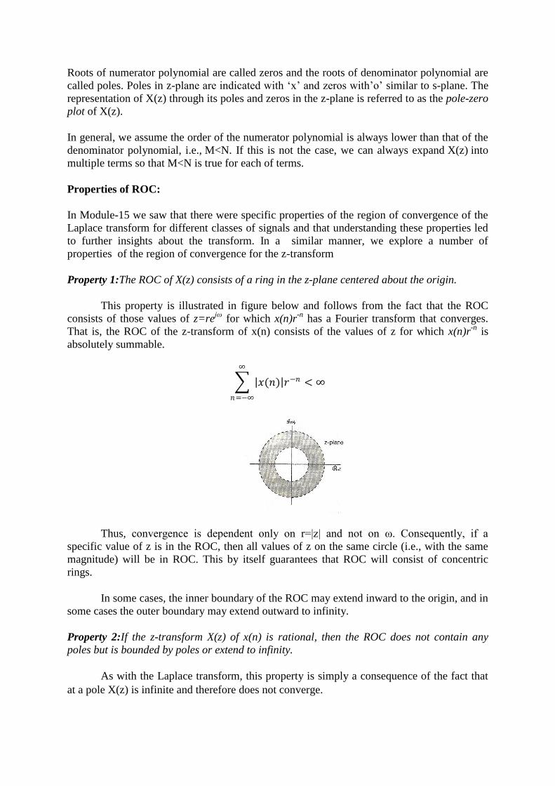
Problem 2:Draw the pole-zero plot and graph the frequency response for the system whose

transfer function is𝐻 𝑧 =𝑧2−0.96𝑧+0.9028

𝑧2−1.56𝑧+0.8109. Is the system both causal and stable?

Solution:

The transfer function can be factored into

𝐻 𝑧 =𝑧2 − 0.96𝑧 + 0.9028

𝑧2 − 1.56𝑧 + 0.8109=

𝑧 − 0.48 + 𝑗0.82 (𝑧 − 0.48 − 𝑗0.82)

𝑧 − 0.78 + 𝑗0.45 (𝑧 − 0.78 − 𝑗0.45)

The Pole-zero diagram is shown below

The magnitude and phase frequency responses of the system are obtained by substituting

z=ejω

and varying the frequency variable ω over a range of 2𝜋. The frequency response plots

are illustrated in Figure below

The system is both causal and stable because all the poles are inside the unit circle

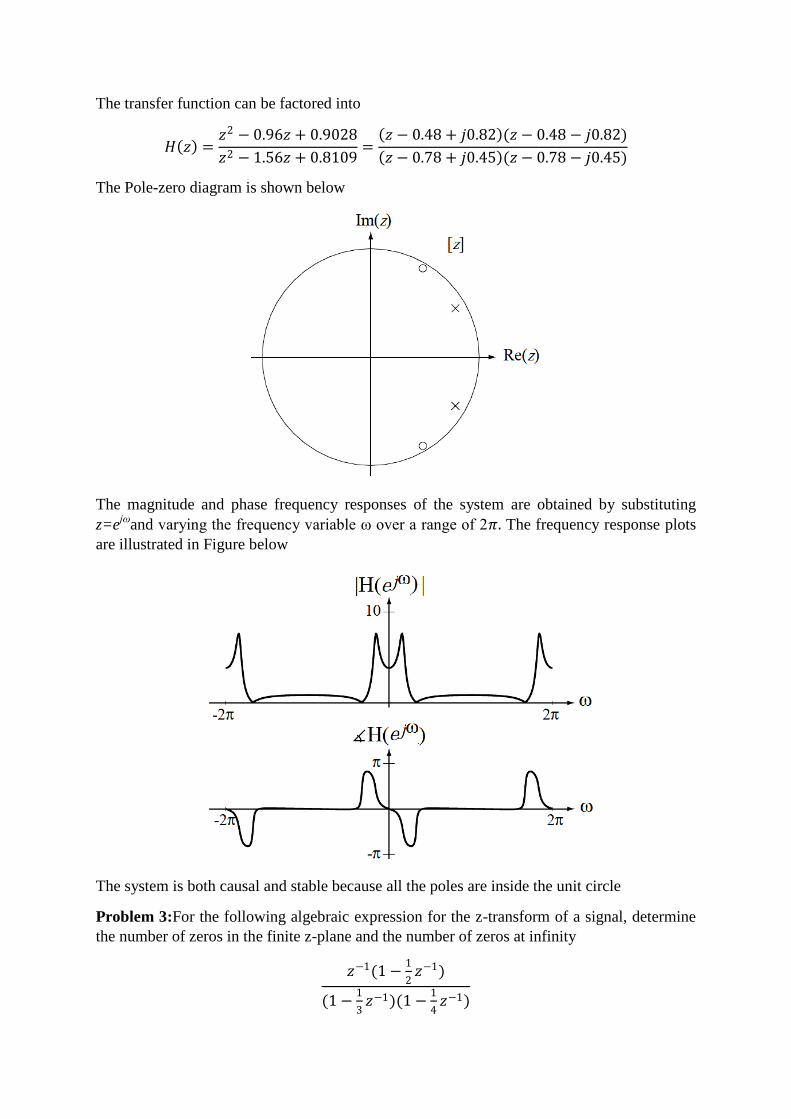
Problem 3:For the following algebraic expression for the z-transform of a signal, determine

the number of zeros in the finite z-plane and the number of zeros at infinity

𝑧−1(1 −1

2𝑧−1)

(1 −1

3𝑧−1)(1 −

1

4𝑧−1)

Solution:

The given z-transform may be written as

𝑋(𝑧) =𝑧 −

1

2

𝑧 −1

3 𝑧 −

1

4

Clearly, X(z) has a zero at z=1/2. Since the order of the denominator polynomial exceeds the

order of the numerator polynomial by 1, X(z) has a zero at infinity. Therefore, X(z) has one

zero in the finite z-plane and one zero at infinity.

Problem 4:Suppose that the algebraic expression for the z-transform of x(n) is

𝑋 𝑧 =1 −

1

4𝑧−1

1 +1

4𝑧−2 1 +

5

4𝑧−1 −

3

8𝑧−2

How many different regions of convergence could correspond to X(z)

Solution:

We may find different signals using given z-transform by choosing different regions of

convergence. The poles of the z-transform are

𝑧𝑜 =1

2𝑗, 𝑧1 = −

1

2𝑗 , 𝑧2 = −

1

2, 𝑧3 =

3

4

Based on these pole locations, we may choose from the following regions of convergence:

(i) 0 < 𝑧 <1

2

(ii) 1

2< 𝑧 <

3

4

(iii) 𝑧 >3

4

Therefore, we may have 3 different signals with given z-transform.

Problem 5: Determine the constraint on r=|z| for1 the following sum to converge

1

2 𝑛+1

𝑧−𝑛∞

𝑛=−1

Solution:

The given summation may be written as 1

2

1

2𝑟−1

𝑛

𝑒−𝑗𝜔𝑛∞𝑛=−1 by replacing z with re

jω. If

𝑟 <1

2, then

1

2𝑟−1 > 1 and the function within the summation grows towards infinity with

increasing n. Also, the summation does not converge. But if 𝑟 >1

2, then the summation

converges

Problem 6:Consider the following system function for stable LTI systems. Without utilizing

the inverse z-transform, determine in each case whether or not the corresponding system is

causal

𝑋 𝑧 =1 −

4

3𝑧−1 +

1

2𝑧−2

𝑧−1 1 −1

2𝑧−1 1 −

1

3𝑧−1

Solution:

For a system to be both causal and stable, the corresponding z-transform must not have any

poles outside the unit circle.

The given z-transform has a pole at infinity. Therefore, it is not causal

Problem 7: Suppose we are given the following five facts about a particular LTI systems „S‟

with impulse response h(n) and z-transform H(z)

1. H(n) is real

2. H(n) is right sided

3. lim𝑧→∞ 𝐻 𝑧 = 1

4. 𝐻 𝑧 has two zeros

5. 𝐻 𝑧 has one of its poles at a nonreal location on the circle defined by |z|=3/4.

Answer the following two questions:

(a) Is „S‟ causal?

(b) Is „S‟ stable?

Solution:

(a) Since lim𝑧→∞ 𝐻 𝑧 = 1, H(z) has not poles at infinity. Furthermore, since h(n) is

given to be right sided, h(n) must be causal.

(b) Since h(n) is causal, the numerator and denominator polynomials of H(z) have the

same order. Since H(z) is given to have two zeros, we may conclude that it also has

two poles.

Since h(n) is real, the poles must occur in conjugate pairs. Also, it is given that

one of the poles lies on the circle defined by |z|=3/4. Therefore, the other pole also lies

on the same circle.

Clearly, the ROC for H(z) will be of the form |z|>3/4, and will include the unit circle.

Therefore, we may conclude that the system is stable

Problem 8: Determine the location of poles and zeros of X(z) for the signal

𝑥 𝑛 = 𝑎𝑛 0 ≤ 𝑛 ≤ 𝑁 − 1,𝑎 > 00 𝑜𝑡ℎ𝑒𝑟𝑤𝑖𝑠𝑒

Solution:

𝑋(𝑧) = 𝑎𝑛𝑧−𝑛 = 𝑎𝑧−1 𝑛 =1 − 𝑎𝑧−1 𝑁

1 − 𝑎𝑧−1=

𝑁−1

𝑛=0

𝑁−1

𝑛=0

1

𝑧𝑁−1

𝑧𝑁 − 𝑎𝑁

𝑧 − 𝑎

Since x(n) is of finite length, it follows from property 3 that the ROC included the entire z-

plane except possible the origin and /or infinity. Since x(n) is zero for n<0, the ROC will

extend to infinity. However, since x(n) is nonzero for some positive values of n, the ROC will

not include the origin. This is evident from the above equation that there is a pole of order N-

1 at z=0. The N roots of the numerator polynomial are at

𝑧𝑘 = 𝑎𝑒𝑗 2𝜋𝑘

𝑁 ,𝑘 = 0,1,2,…𝑁 − 1

The root for k=0 cancels the pole at z=a. Consequently, there are no poles other than at the

origin. The remaining zeros are at

𝑧𝑘 = 𝑎𝑒𝑗 2𝜋𝑘

𝑁 ,𝑘 = 1,2,…𝑁 − 1

The pole zero pattern is shown below for 0 < a < 1

Problem 9: Show all the possible ROCs that can relate to the function

𝑋 𝑧 =1

1 −1

3𝑧−1 1 − 2𝑧−1

Solution:

Figure (a) represents the pole zero plot

Figure (b) is the pole-zero pattern with ROC if x(n) is right sided

Figure (c) is the pole-zero pattern with ROC if x(n) is left sided

Figure (d) is the pole-zero pattern with ROC if x(n) is two sided

In all the cases, the zero at the origin is a second order zero

Problem 10:Determine the z-transform for each of the following sequences and indicate the

region of convergence. Indicate whether Fourier transform of the sequence exists.

a) 𝛿(𝑛 + 5)

b) 𝛿(𝑛 − 5)

Solution:

a) For 𝑥 𝑛 = 𝛿(𝑛 + 5), 𝑋 𝑧 = 𝑧5, ROC: All z except at z=∞

The Fourier transform exists because the ROC includes the unit circle

b) For 𝑥 𝑛 = 𝛿(𝑛 + 5), 𝑋 𝑧 = 𝑧−5, ROC: All z except at z=0

The Fourier transform exists because the ROC includes the unit circle

Assignment:

Problem 1 : Find the z-transform and ROC of the signal𝑥 𝑛 = 4 5 𝑛 − 3 4 𝑛 𝑢(𝑛)

Problem 2:Plot the ROC in z-plane for the signal𝑥 𝑛 = 𝑎𝑛𝑢 𝑛 + 𝑏𝑛𝑢(−𝑛 − 1), if

(i) |a| > |b|

(ii) |a| < |b|

Problem 3:Let 𝑥 𝑛 = −1 𝑛𝑢 𝑛 + 𝛼𝑛𝑢(𝑛 − 𝑛𝑜)

Determine the constraints on the complex number 𝛼 and the integer no, given that the ROC of

X(z) is 1 < |z| < 2

Problem 4:Consider the signal𝑥 𝑛 = 1

3 𝑛

cos 𝑛𝜋

4 , 𝑛 ≤ 0

0 𝑛 > 0

Determine the poles and ROC for X(z)

Problem 5: For the following algebraic expression for the z-transform of a signal, determine

the number of zeros in the finite z-plane and the number of zeros at infinity

𝑧−2(1 − 𝑧−1)

(1 −1

4𝑧−1)(1 +

1

4𝑧−1)

Problem 6: Let x(n) be an absolutely summable signal with rational z-transform X(z). If X(z)

is known to have a pole at z=1/2, could x(n) be

a) A finite duration signal?

b) A left sided signal?

c) A right sided signal?

d) A two sided signal?

Problem 7: Determine the constraint on r=|z| for1 the following sum to converge

1

2 −𝑛+1

𝑧𝑛∞

𝑛=1

Problem 8: Let x(n) be asignal whose rational z-transform X(z) contains a pole at z=1/2.

Given that 𝑥1 𝑛 = 1

4 𝑛

𝑥(𝑛) is absolutely summable and 𝑥2 𝑛 = 1

8 𝑛

𝑥(𝑛) is not

absolutely summable, determine whether x(n) is left sided, right sided or two sided.

Problem 9: Consider the following system function for stable LTI systems. Without utilizing

the inverse z-transform, determine in each case whether the corresponding system is causal.

𝑋 𝑧 =𝑧 + 1

𝑧 +4

3−

1

2𝑧−2 −

2

3𝑧−3

Problem 10: If 𝑥[𝑛] = (1/3) 𝑛 − (1/2)𝑛𝑢[𝑛], then find the region of convergence

(ROC) of itsz -transform in the z -plane.

Simulation:

Pole-Zero Plot:

A Pole-Zero plot displays the “poles” and “zeros” of the rational transform byplacing

an „x‟ at each pole location and an „o‟ at each zero location in thecomplex z-plane.

Poles and zeros can be found out by using tf2zpfunction and pole-zero plot is

obtained using zplane function in MATLAB.

For Example:

% Pole – Zero Map in Z- Domain

clc;

clear all;

close all;

%z-domain LTI system

%y(n)=(3/8)y(n-1)+(2/3)y(n-2)+x(n)+(1/4)x(n-1)

a= input('Enter the Numerator coefficients');

b = input('Enter the Denominator coefficients');

[z1,p1,k]=tf2zp(a,b);

disp('pole locations are');p1

disp('zero locations are');z1

figure,

zplane(a,b);

INPUT:

Enter the Numerator coefficients[1,1/4]

Enter the Denominator coefficients[1 -3/8,-2/3]

OUTPUT:

pole locations are

p1 =

1.0252

-0.6502

zero locations are

z1 =

-0.2500

Practice:

Locate poles and zeros in z-plane using MATLAB for the following function

𝐻(𝑧) =𝑧3 − 0.8𝑧2

z3 − 1.1 z2 − 0.22 z + 0.06

References:

[1] Alan V.Oppenheim, Alan S.Willsky and S.Hamind Nawab, “Signals & Systems”, Second

edition, Pearson Education, 8th

Indian Reprint, 2005.

[2] M.J.Roberts, “Signals and Systems, Analysis using Transform methods and MATLAB”,

Second edition,McGraw-Hill Education,2011

[3] John R Buck, Michael M Daniel and Andrew C.Singer, “Computer explorations in

Signals and Systems using MATLAB”,Prentice Hall Signal Processing Series

[4] P Ramakrishna rao, “Signals and Systems”, Tata McGraw-Hill, 2008

[5] Tarun Kumar Rawat, “Signals and Systems”, Oxford University Press,2011