STA 2023

Module 10 Comparing Two Proportions

Learning Objectives

Upon completing this module, you should be able to:

1.  Perform large-sample inferences (hypothesis test and confidence intervals) to compare two population proportions.

2.  Describe the relationship between the sample sizes, confidence level, and margin of error for a confidence interval for the difference between two population proportions.

3.  Determine the sample size required for a specified confidence level and margin of error for the estimate of the difference between two population proportions.

Population Proportions

In this module, we are going to learn how to compare two population proportions.

Remember, a population proportion, p is simply the percentage of a population that has a specified attribute.

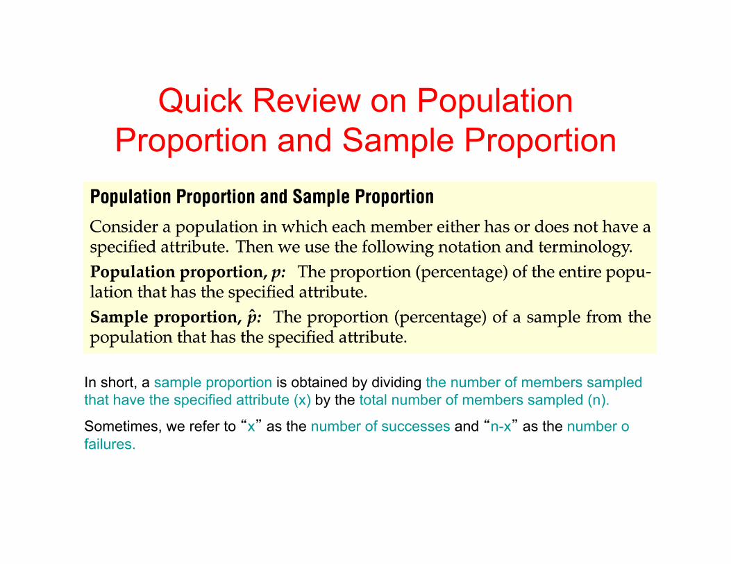
Quick Review on Population Proportion and Sample Proportion

In short, a sample proportion is obtained by dividing the number of members sampled that have the specified attribute (x) by the total number of members sampled (n).

Sometimes, we refer to “x” as the number of successes and “n-x” as the number o failures.

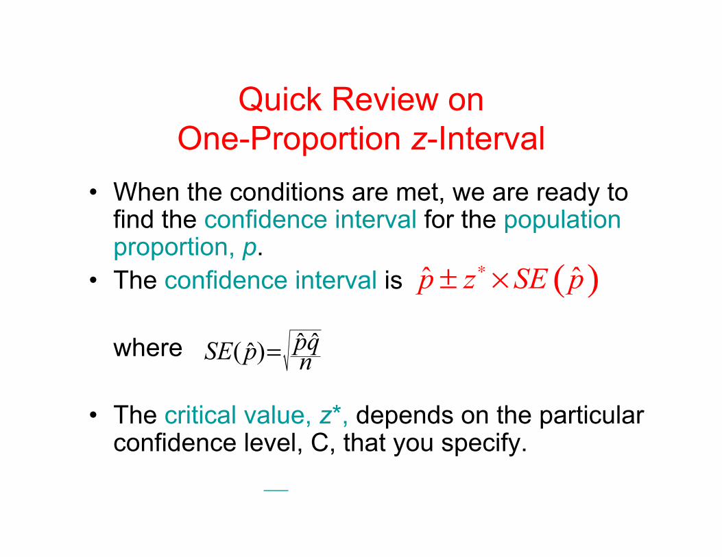
Quick Review on One-Proportion z-Interval

•  When the conditions are met, we are ready to find the confidence interval for the population proportion, p.

•  The confidence interval is

where •  The critical value, z*, depends on the particular

confidence level, C, that you specify.

ˆ ˆ( )ˆ pqSE p n=

( )ˆ ˆp z SE p∗± ×

Comparing Two Proportions

•  Comparisons between two percentages are much more common than questions about isolated percentages. And they are more interesting.

•  We often want to know how two groups differ, whether a treatment is better than a placebo control, or whether this year’s results are better than last year’s.

Another Ruler

•  In order to examine the difference between two proportions, we need another ruler—the standard deviation of the sampling distribution model for the difference between two proportions.

•  Recall that standard deviations don’t add, but variances do. In fact, the variance of the sum or difference of two independent random variables is the sum of their individual variances.

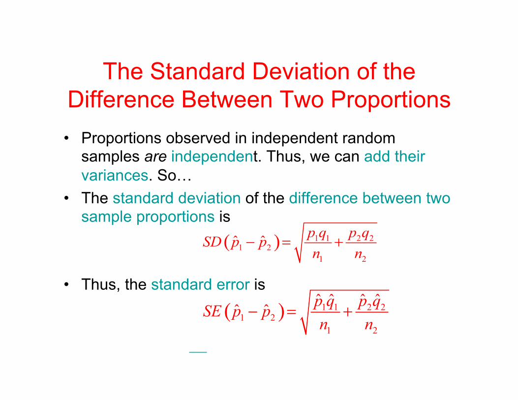
The Standard Deviation of the Difference Between Two Proportions •  Proportions observed in independent random

samples are independent. Thus, we can add their variances. So…

•  The standard deviation of the difference between two sample proportions is

•  Thus, the standard error is

( ) 1 1 2 21 2

1 2

ˆ ˆ p q p qSD p pn n

− = +

( ) 1 1 2 21 2

1 2

ˆ ˆ ˆ ˆˆ ˆ p q p qSE p pn n

− = +

Assumptions and Conditions

•  Independence Assumptions: –  Randomization Condition: The data in each group

should be drawn independently and at random from a homogeneous population or generated by a randomized comparative experiment.

–  The 10% Condition: If the data are sampled without replacement, the sample should not exceed 10% of the population.

–  Independent Groups Assumption: The two groups we’re comparing must be independent of each other.

Assumptions and Conditions (cont.)

•  Sample Size Condition: – Each of the groups must be big enough… – Success/Failure Condition: Both groups

are big enough that both successes and failures are at least 5 have been observed in each.

The Sampling Distribution

•  We already know that for large enough samples, each of our proportions has an approximately Normal sampling distribution.

•  The same is true of their difference.

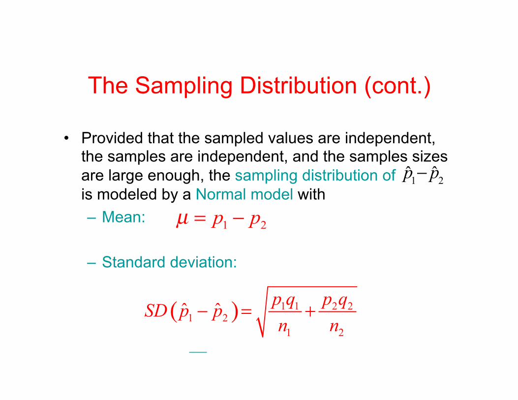
The Sampling Distribution (cont.)

•  Provided that the sampled values are independent, the samples are independent, and the samples sizes are large enough, the sampling distribution of is modeled by a Normal model with –  Mean:

–  Standard deviation:

1 2p pµ = −

1 2ˆ ˆp p−

( ) 1 1 2 21 2

1 2

ˆ ˆ p q p qSD p pn n

− = +

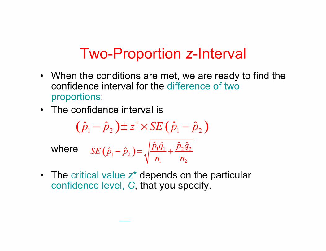
Two-Proportion z-Interval •  When the conditions are met, we are ready to find the

confidence interval for the difference of two proportions:

•  The confidence interval is

where

•  The critical value z* depends on the particular confidence level, C, that you specify.

( ) 1 1 2 21 2

1 2

ˆ ˆ ˆ ˆˆ ˆ p q p qSE p pn n

− = +

( ) ( )1 2 1 2ˆ ˆ ˆ ˆp p z SE p p∗− ± × −

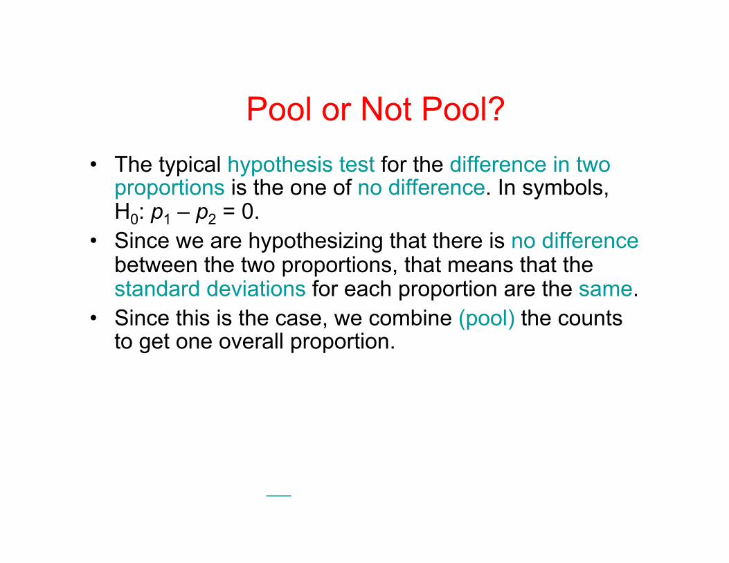
Pool or Not Pool? •  The typical hypothesis test for the difference in two

proportions is the one of no difference. In symbols, H0: p1 – p2 = 0.

•  Since we are hypothesizing that there is no difference between the two proportions, that means that the standard deviations for each proportion are the same.

•  Since this is the case, we combine (pool) the counts to get one overall proportion.

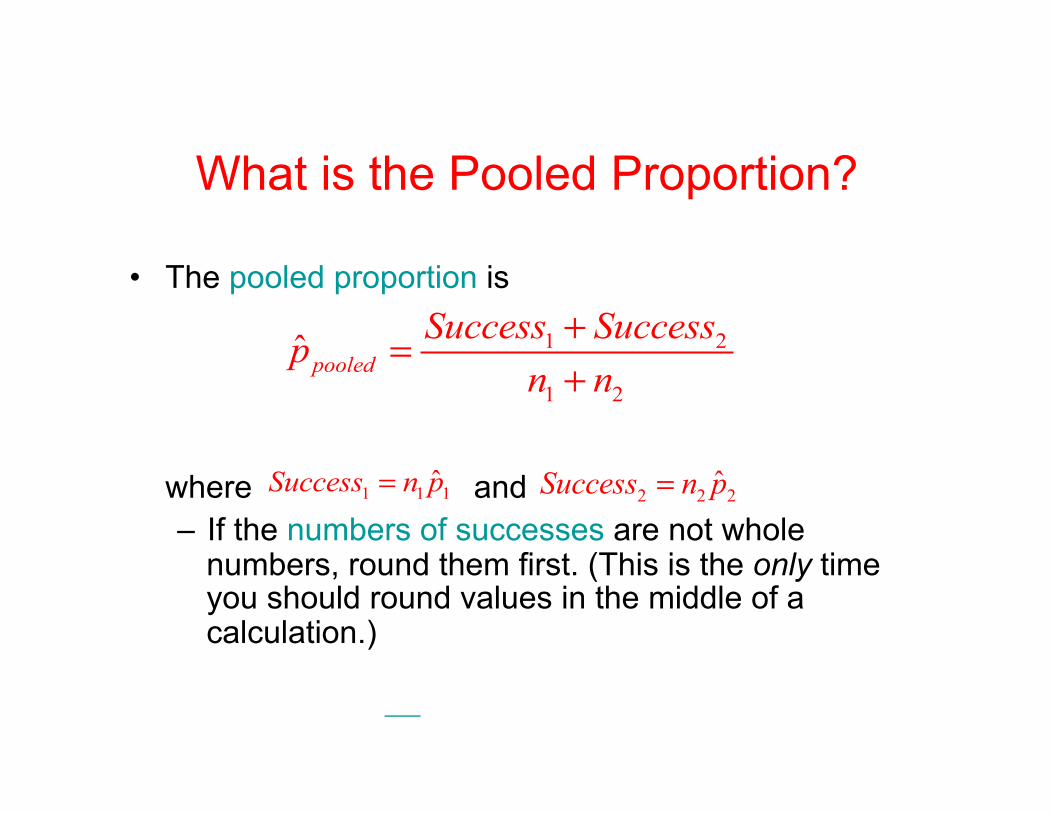
What is the Pooled Proportion?

•  The pooled proportion is

where and –  If the numbers of successes are not whole

numbers, round them first. (This is the only time you should round values in the middle of a calculation.)

1 2

1 2

ˆ pooledSuccess Success

pn n+=+

1 1 1ˆSuccess n p= 2 2 2ˆSuccess n p=

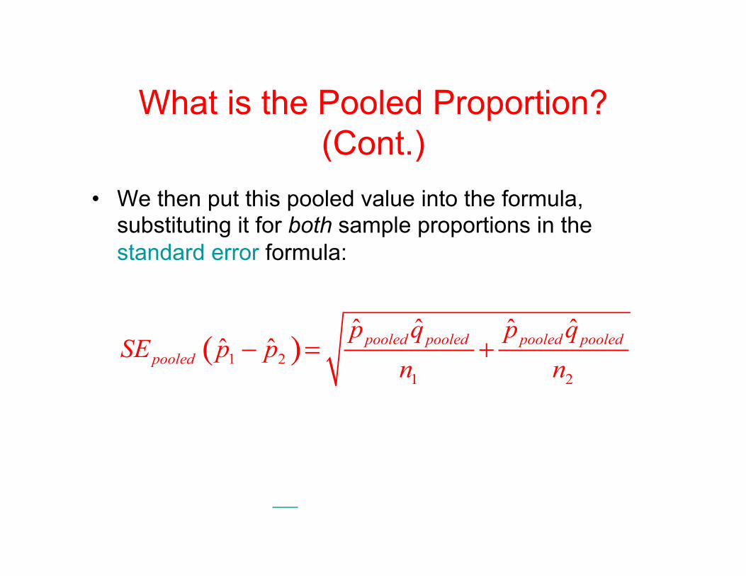
What is the Pooled Proportion? (Cont.)

•  We then put this pooled value into the formula, substituting it for both sample proportions in the standard error formula:

( )1 21 2

ˆ ˆ ˆ ˆˆ ˆ pooled pooled pooled pooled

pooled

p q p qSE p p

n n− = +

Compared to What?

•  We’ll reject our null hypothesis if we see a large enough difference in the two proportions.

•  How can we decide whether the difference we see is large? –  Just compare it with its standard deviation.

•  Unlike previous hypothesis testing situations, the null hypothesis doesn’t provide a standard deviation, so we’ll use a standard error (here, pooled).

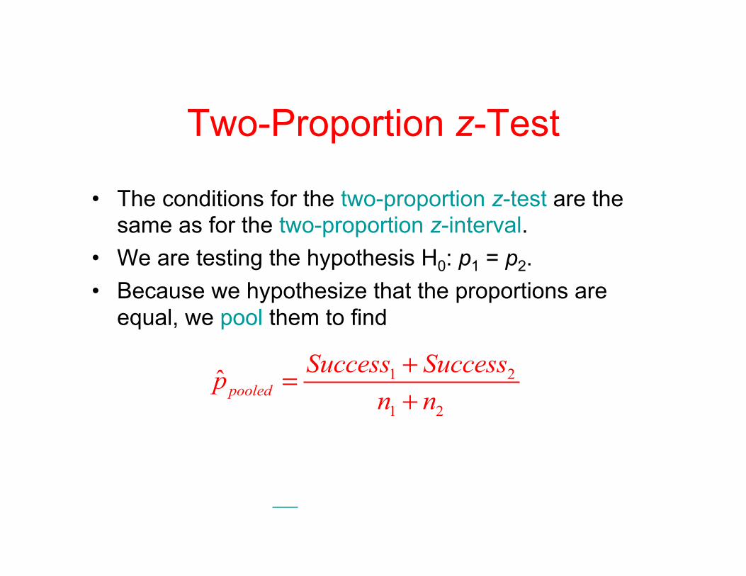
Two-Proportion z-Test

•  The conditions for the two-proportion z-test are the same as for the two-proportion z-interval.

•  We are testing the hypothesis H0: p1 = p2. •  Because we hypothesize that the proportions are

equal, we pool them to find

1 2

1 2

ˆ pooledSuccess Success

pn n+=+

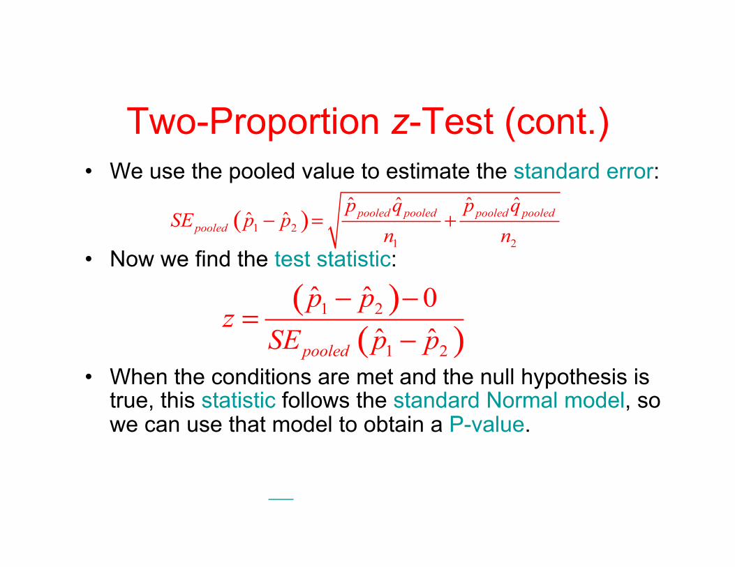
Two-Proportion z-Test (cont.) •  We use the pooled value to estimate the standard error:

•  Now we find the test statistic:

•  When the conditions are met and the null hypothesis is true, this statistic follows the standard Normal model, so we can use that model to obtain a P-value.

( )1 21 2

ˆ ˆ ˆ ˆˆ ˆ pooled pooled pooled pooled

pooled

p q p qSE p p

n n− = +

( )( )

1 2

1 2

ˆ ˆ 0ˆ ˆpooled

p pzSE p p

− −=

−

Quick Review Let’s look at the following one more time:

•  How to find one proportion z-interval? •  How to perform a one proportion z-test? •  What is the sampling distribution of the difference

between two sample proportions? •  How to perform a two proportion z-test? •  How to find a two proportion z-interval?

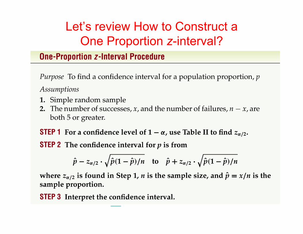
Let’s review How to Construct a One Proportion z-interval?

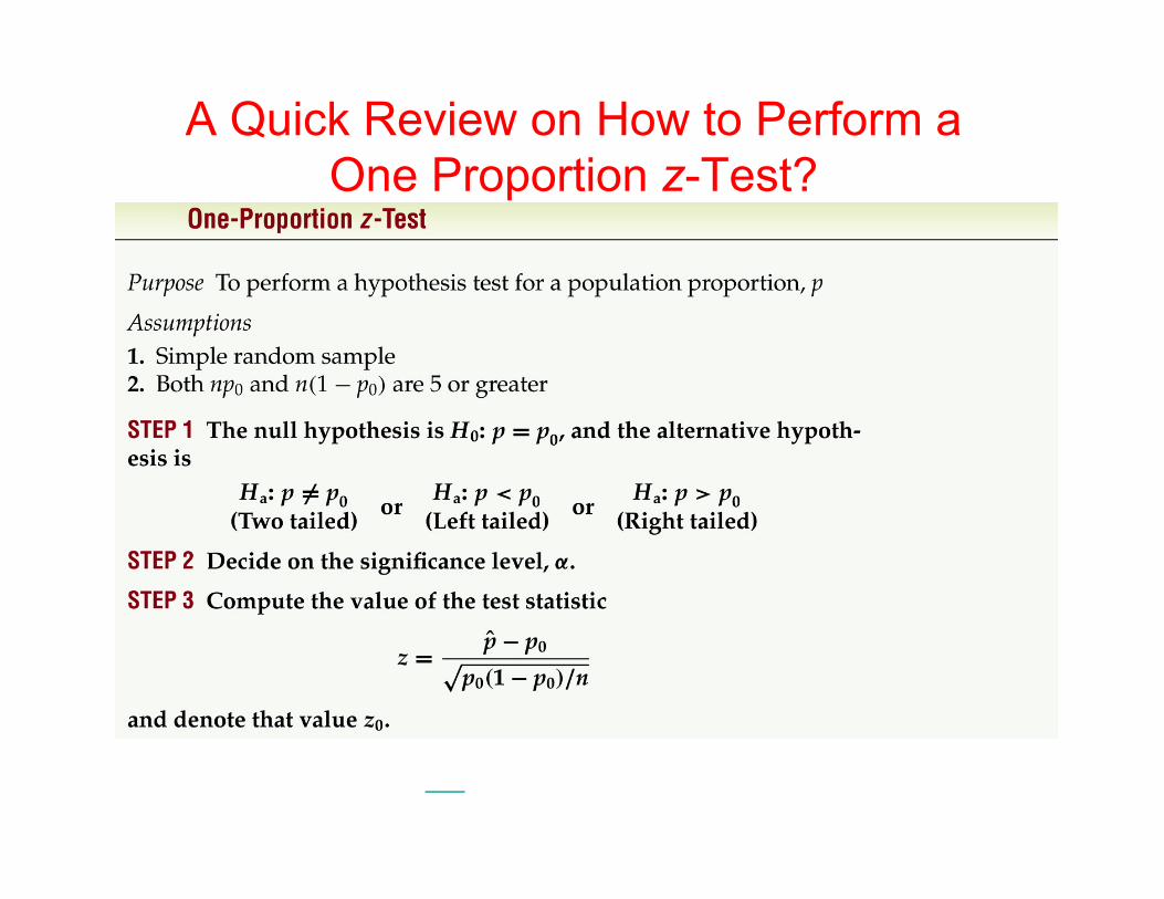
A Quick Review on How to Perform a One Proportion z-Test?

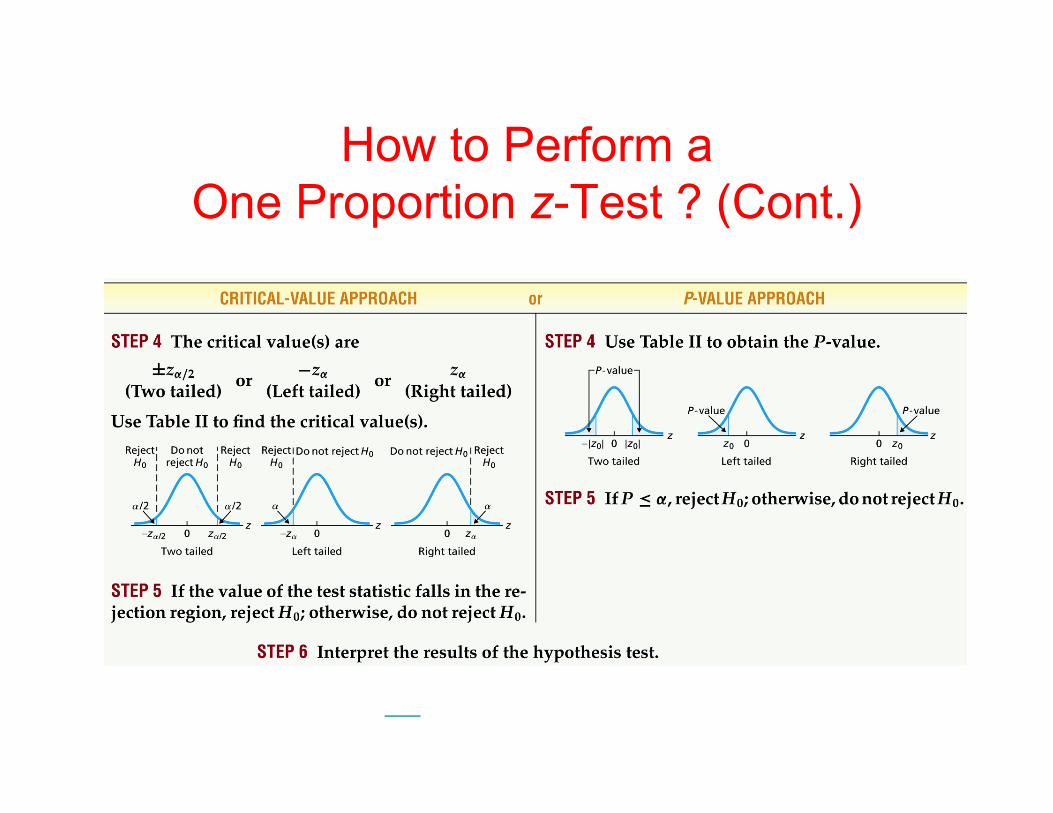
How to Perform a One Proportion z-Test ? (Cont.)

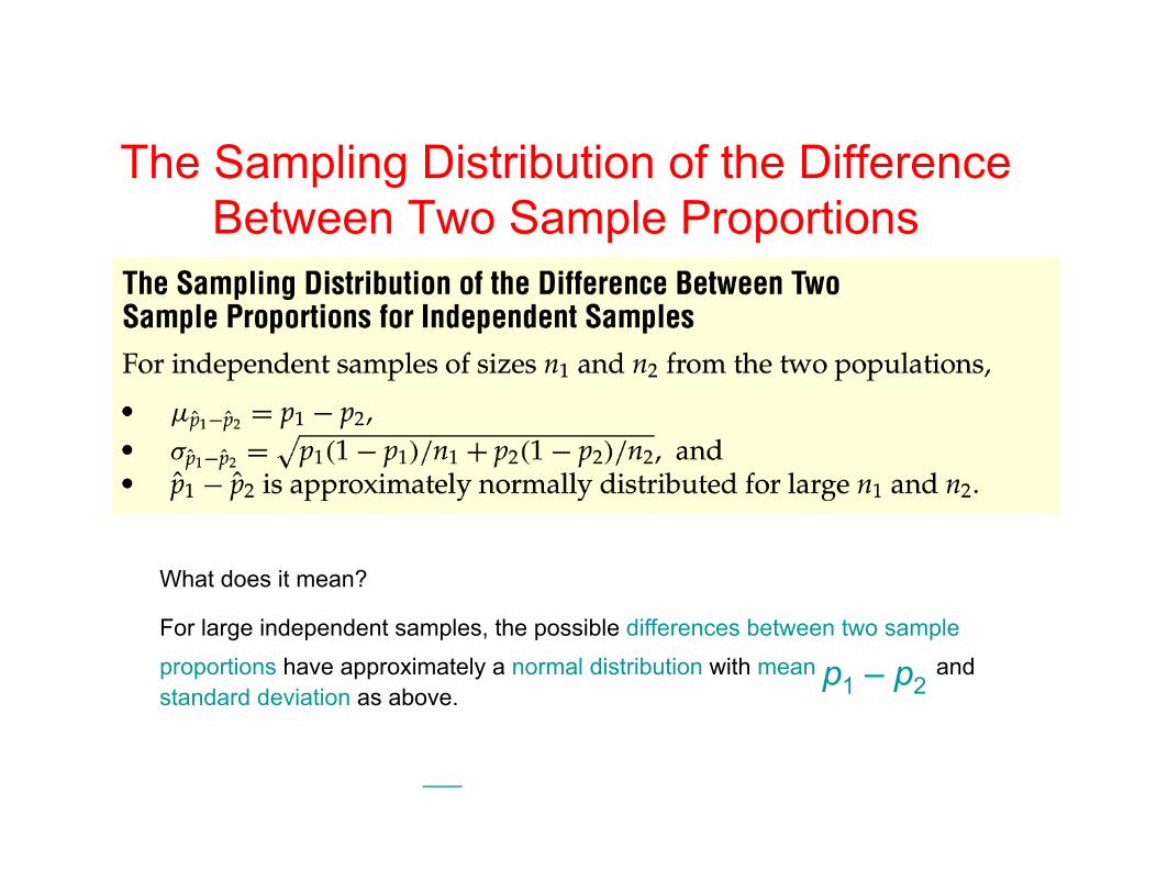
The Sampling Distribution of the Difference Between Two Sample Proportions

What does it mean?

For large independent samples, the possible differences between two sample proportions have approximately a normal distribution with mean p1 – p2 and standard deviation as above.

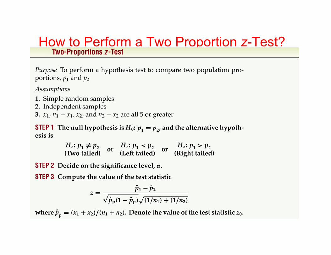
How to Perform a Two Proportion z-Test?

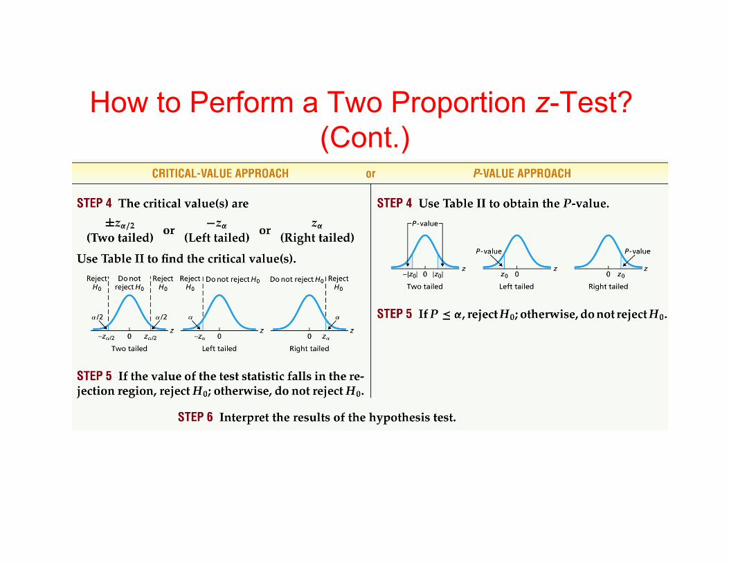
How to Perform a Two Proportion z-Test? (Cont.)

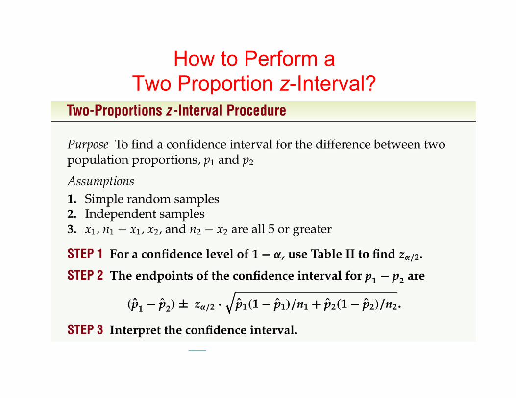
How to Perform a Two Proportion z-Interval?

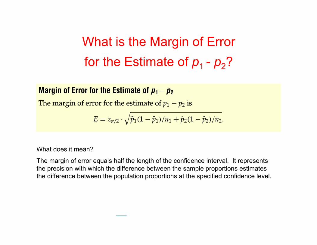
What is the Margin of Error for the Estimate of p1 - p2?

What does it mean?

The margin of error equals half the length of the confidence interval. It represents the precision with which the difference between the sample proportions estimates the difference between the population proportions at the specified confidence level.

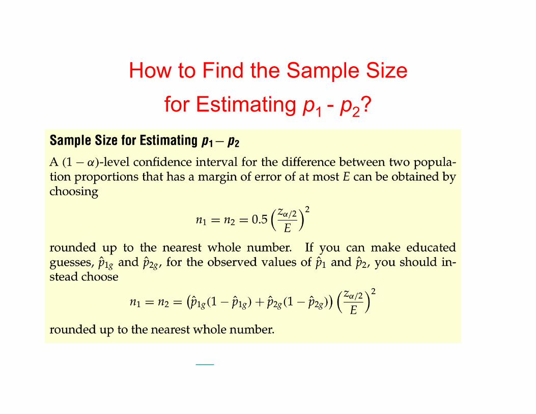
How to Find the Sample Size for Estimating p1 - p2?

What Can Go Wrong?

Don’t Misstate What the Interval Means: •  Don’t suggest that the parameter varies. •  Don’t claim that other samples will agree with yours. •  Don’t be certain about the parameter. •  Don’t forget: It’s the parameter (not the statistic). •  Don’t claim to know too much. •  Do take responsibility (for the uncertainty).

What Can Go Wrong? (cont.)

Margin of Error Too Large to Be Useful: •  We can’t be exact, but how precise do we need to

be? •  One way to make the margin of error smaller is to

reduce your level of confidence. (That may not be a useful solution.)

•  You need to think about your margin of error when you design your study. –  To get a narrower interval without giving up

confidence, you need to have less variability. –  You can do this with a larger sample…

What Can Go Wrong? (cont.)

Violations of Assumptions: •  Watch out for biased sampling. •  Think about independence.

What Can Go Wrong? (cont.)

•  Don’t base your null hypothesis on what you see in

the data. –  Think about the situation you are investigating and

develop your null hypothesis appropriately. •  Don’t base your alternative hypothesis on the data,

either. –  Again, you need to Think about the situation.

What Can Go Wrong? (Cont.) •  Don’t use two-sample proportion methods when the

samples aren’t independent. –  These methods give wrong answers when the

independence assumption is violated. •  Don’t apply inference methods when there was no

randomization. –  Our data must come from representative random

samples or from a properly randomized experiment. •  Don’t interpret a significant difference in proportions

causally. –  Be careful not to jump to conclusions about causality.

What have we learned?

We have learned to:

1.  Perform large-sample inferences (hypothesis test and confidence intervals) to compare two population proportions.

2.  Describe the relationship between the sample sizes, confidence level, and margin of error for a confidence interval for the difference between two population proportions.

3.  Determine the sample size required for a specified confidence level and margin of error for the estimate of the difference between two population proportions.

Credit

Some of these slides have been adapted/modified in part/whole from the slides of the following textbooks.

•  Weiss, Neil A., Introductory Statistics, 8th Edition •  Bock, David E., Stats: Data and Models, 3rd Edition