Modulation and Coding Tradeoffs - Egloospds8.egloos.com/pds/200805/13/35/09_Modulation_and... ·...
54
0 College of Information & Communications The world goes wireless! Prepared by Sung Ho Cho Hanyang University Modulation and Coding Tradeoffs
Transcript of Modulation and Coding Tradeoffs - Egloospds8.egloos.com/pds/200805/13/35/09_Modulation_and... ·...

0
College of Information & Communications
The world goes wireless! Prepared by Sung Ho Cho
Hanyang University
Modulation and Coding Tradeoffs

1
College of Information & Communications
The world goes wireless! Prepared by Sung Ho Cho
Hanyang University
Contents1. Design Goals 2. Error Probability Plane3. Nyquist Minimum Bandwidth4. Shannon‐Hartley Capacity Theorem5. Bandwidth‐Efficiency Plane6. Modulation and Coding Tradeoffs7. Design Steps of Communication Systems8. Bandwidth‐Efficient Modulation9. Modulation and Coding for Bandlimited Channels

2
College of Information & Communications
The world goes wireless! Prepared by Sung Ho Cho
Hanyang University
1. Design Goals
3
College of Information & Communications
The world goes wireless! Prepared by Sung Ho Cho
Hanyang University
Design Goals
Maximum transmission bit rate RMinimum probability of bit error PBMinimum required power or Eb/N0
Minimum system bandwidth WMinimum system complexityMaximum system utilization
For reliable serviceFor a maximum number of usersWith minimum delayWith maximum resistance to interference
Tradeoff

4
College of Information & Communications
The world goes wireless! Prepared by Sung Ho Cho
Hanyang University
Constraints and Limitations
Nyquist theoretical minimum bandwidth requirementShannon‐Hartley capacity theorem (and Shannon limit)Government regulations (e.g., frequency allocations)Technological limitations (e.g., state‐of‐the‐art components)Other system requirements (e.g., satellite orbits)
Two major performance planes:Error probability planeBandwidth efficiency plane
5
College of Information & Communications
The world goes wireless! Prepared by Sung Ho Cho
Hanyang University
2. Error Probability Plane

6
College of Information & Communications
The world goes wireless! Prepared by Sung Ho Cho
Hanyang University
Bit Error Probability versus Eb/N0Coherent MFSK: Coherent MPSK:
PB↔WEb/N0: fixed
PB↔ EW: fixed
b/N0
Eb/N0 ↔WPB: fixed
Equi‐bandwidth Curves

7
College of Information & Communications
The world goes wireless! Prepared by Sung Ho Cho
Hanyang University
3. Nyquist Minimum Bandwidth

8
College of Information & Communications
The world goes wireless! Prepared by Sung Ho Cho
Hanyang University
Filtering Aspects of ISI
ISI for a typical baseband digital system:
Equivalent model:
Transmitting filter Channel Receiving filter
The tail of a pulse smears into adjacent symbol intervals.
Hr(f)Ht(f) Hc(f)

9
College of Information & Communications
The world goes wireless! Prepared by Sung Ho Cho
Hanyang University
System Transfer Function for Baseband Channel
System Transfer Function, H(f), and ideal Nyquist pulse, h(t)
If each pulse of a received sequence is of the form sinc(t/T), then the pulses can be detected without ISI.
Sampling at the receiver at every T sec.

10
College of Information & Communications
The world goes wireless! Prepared by Sung Ho Cho
Hanyang University
Nyquist Minimum Bandwidth
The theoretical minimum bandwidth (Nyquist bandwidth) needed for the baseband transmission of Rs symbols/s without ISI is Rs/2 Hz.
The maximum possible symbol transmission rate per hertz is 2 symbols/s/Hz.
In practice, the Nyquist minimum bandwidth is expanded by about 10% to 40% due to the constraints of real filters.
Typical baseband digital communication throughput is reduced from the ideal 2 symbols/s/Hz down to the range of about 1.8 to 1.4 symbols/s/Hz.
Bandwidth Efficiency: R/Wmeasured in bits/s/HzA measurement of data throughput per hertz of bandwidth.Ex) MPSK system:
For a fixed bandwidth W, as k increases, the allowable data rate Rincreases, and thus R/W increases at the expense of large Eb/N0.

11
College of Information & Communications
The world goes wireless! Prepared by Sung Ho Cho
Hanyang University
4. Shannon‐Hartley Capacity Theorem
C.E. Shannon,”A Mathematical Theory of Communication,”
BSTJ, Vol.27, pp.379‐423, 1948.

12
College of Information & Communications
The world goes wireless! Prepared by Sung Ho Cho
Hanyang University
System Capacity
Shannon‐Hartley Capacity Theorem:
C: System capacity for an AWGN channelW: BandwidthS: Average received signal power (S = EbR)N: Average noise power (N = N0W)
It is theoretically possible to transmit information over an AWGN channel at any rate R≤C, with an arbitrarily small error probability by using a sufficiently complicated coding scheme.
Shannon’s work shows that the values of S, N, and W set a limit on transmission rate, not an error probability.
(bits/s)

13
College of Information & Communications
The world goes wireless! Prepared by Sung Ho Cho
Hanyang University
Normalized Channel Capacity/Bandwidth vs. SNR
Normalized channel capacity vs. SNR Normalized channel bandwidth vs. SNR
2log 1C SW N
⎛ ⎞= +⎜ ⎟⎝ ⎠

14
College of Information & Communications
The world goes wireless! Prepared by Sung Ho Cho
Hanyang University
Normalized Channel Capacity vs. Eb/N0Suppose that the transmission bit rate, R = channel capacity, C
This is the case when R=C.
0N N W=
0
// /
b bE S T S R S WN N W N W N R
⎛ ⎞= = = ⎜ ⎟⎝ ⎠
0
bES RN N W
⎛ ⎞= ⎜ ⎟⎝ ⎠
2 20
log 1 log 1 bEC S CW N N W
⎛ ⎞⎛ ⎞ ⎛ ⎞= + = +⎜ ⎟⎜ ⎟ ⎜ ⎟⎝ ⎠ ⎝ ⎠⎝ ⎠
/
02 1C W bE C
N W⎛ ⎞= + ⎜ ⎟⎝ ⎠
( )/
02 1C WbE W
N C= −
If R = C

15
College of Information & Communications
The world goes wireless! Prepared by Sung Ho Cho
Hanyang University
Shannon LimitDefinition:
The limit of Eb/N0 below which there can be no error‐free communication at any information rateShannon’s work provides a theoretical proof for the existence of codes that could improve the PB performance, or reduce the Eb/N0 required.Today, as much as 10 dB improvement is realizable with turbo code.
Mathematical limit:
We use the identity:
Let
Then
As C/W→0 or x→0, we have
or
or
Again, this is the case when R=C.

16
College of Information & Communications
The world goes wireless! Prepared by Sung Ho Cho
Hanyang University
Entropy, H
Definition:A metric for measuring the average amount of information per source output
For a binary case:
where pi is the probability of the i‐th output and .
Maximum entropy when events occur equally likely.

17
College of Information & Communications
The world goes wireless! Prepared by Sung Ho Cho
Hanyang University
Properties of EntropyThe unit for H is average bit per event.
It is a measure of information content, and should not be confused with the term bit, meaning “binary digit.”
The term “entropy” has the same uncertainty connotation as it does in certain formulations of statistical mechanics.
The uncertainty in the event becomes maximum when the information source has equally likely possibilities.If we know the result before the event happens, then the result conveys no additional information.
Example: English alphabet If 26 letters occur with equal likelihood:
But, if
“There is a way of encoding the English language
with a fewer number of bits per character on the average.”

18
College of Information & Communications
The world goes wireless! Prepared by Sung Ho Cho
Hanyang University
Equivocation, H(X|Y) (1/2)Shannon uses a correction factor, call equivocation, to characterize the uncertainty in the received signal.Equivocation is defined as the conditional entropy of the message X, given Y, such that
where X = transmitted source messageY = received signalP(X,Y) = joint probability of X and YP(X|Y) = conditional probability of X given Y
For an error‐free channel, H(X|Y) = 0, because having received Y, there is no uncertainty about the message X, (i.e., P(X|Y) = 1). For a channel with a nonzero probability of symbol error, H(X|Y) > 0, because the channel introduces uncertainty.

19
College of Information & Communications
The world goes wireless! Prepared by Sung Ho Cho
Hanyang University
Equivocation, H(X|Y) (2/2)Example: For a binary sequence, X,
Let the a priori source probabilities be P(X=1) = P(X=0) = ½.Let the bit error probability at the receiver become PB = 0.01.
Then the equivocation H(X|Y) becomes
( )
( ) ( )
( ) ( )
( ) ( )
2
2 2
2 2
2 2
2 2
2 2
2
( ) ( ) log ( )
(0) (0 0)log (0 0) (1 0)log (1 0)
(1) (0 1)log (0 1) (11)log (11)
1 1 log 1 log2
1 log 1 log 12
1 log 1 log
0.99log 0.
Y X
B B B B
B B B B
B B B B
H X Y P Y P X Y P X Y
P P P P P
P P P P P
P P P P
P P P P
P P P P
= −
= − +⎡ ⎤⎣ ⎦− +⎡ ⎤⎣ ⎦
= − − − +⎡ ⎤⎣ ⎦
− + − −⎡ ⎤⎣ ⎦
= − − − +⎡ ⎤⎣ ⎦= −
∑ ∑
( ) ( )299 0.01log 0.01
0.081 bit/received symbol
+⎡ ⎤⎣ ⎦=
“The channel introduces 0.081 bit of uncertainty to each received symbol.”

20
College of Information & Communications
The world goes wireless! Prepared by Sung Ho Cho
Hanyang University
Effective Entropy, Heff
Effective entropy, Heff, is used to characterize the average effective information content, defined by
Example: For a system transmitting equally likely binary symbols,The entropy H(X) = 1.If the symbols are received with PB = 0.01, the equivocation H(X|Y) =0.081.Then the effective entropy becomes
Thus, if the binary symbol rate is given by R = 1000 symbols/s, the effective information bit rate Reff can then be written as
Note that in the extreme case, where PB = 0.5, we have
Heff = 0
Reff = 0 “The effective information bit rate is zero!”

21
College of Information & Communications
The world goes wireless! Prepared by Sung Ho Cho
Hanyang University
5. Bandwidth‐Efficiency Plane

22
College of Information & Communications
The world goes wireless! Prepared by Sung Ho Cho
Hanyang University
PB↔ R/WEb/N0: fixed
PB↔ Eb/N0R/W: fixed
Eb/N0 ↔ R/WPB: fixed
Equi‐error probability curves
Ideal performance
Bandwidth‐Efficiency Plane (R/W vs. Eb/N0)
( ) 22
loglogs ss
MR k R M RT
= = =
2logR MW
=
1
s
WT
≈
2log MRW M
=
s
MWT
≈
Reflects how efficiently the bandwidth resource is utilized.
Bandwidth‐efficiency plane at PB=10‐5:
For coherent MPSK:
For Noncoherent MFSK:

23
College of Information & Communications
The world goes wireless! Prepared by Sung Ho Cho
Hanyang University
6. Modulation and Coding Tradeoffs

24
College of Information & Communications
The world goes wireless! Prepared by Sung Ho Cho
Hanyang University
Error‐Probability Plane vs. Bandwidth‐Efficiency Plane
Error Probability Plane
G: gained, C: cost, F: fixed
Bandwidth‐Efficiency Plane“Useful for examining power‐limited systems.” “Useful for examining bandwidth‐limited systems.”

25
College of Information & Communications
The world goes wireless! Prepared by Sung Ho Cho
Hanyang University
7. Design Steps of Communication Systems

26
College of Information & Communications
The world goes wireless! Prepared by Sung Ho Cho
Hanyang University
Before Designing Communication Systems…
Need description of the channel:Received powerAvailable bandwidthNoise statisticsOther impairments, such as fading
Need definition of the system requirements:Data rateError performanceTradeoff between bandwidth ↔ power
Given the channel description, we determine design choices that best match the channel and meet the performance requirements.
27
College of Information & Communications
The world goes wireless! Prepared by Sung Ho Cho
Hanyang University
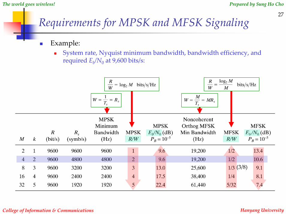
Requirements for MPSK and MFSK Signaling
Example:System rate, Nyquist minimum bandwidth, bandwidth efficiency, and required Eb/N0 at 9,600 bits/s:
(3/8)

28
College of Information & Communications
The world goes wireless! Prepared by Sung Ho Cho
Hanyang University
Example 1: Bandwidth‐Limited Uncoded SystemAssumptions:
AWGN radio channelAvailable bandwidth: W = 4,000 HzRatio of received signal power to noise power spectral density: Pr/N0 = 53 dB‐HzRequired data rate: R = 9,600 bits/sRequired bit error probability: PB = 10‐5
Design steps:Received Eb/N0:
Use the relationship between Pr/N0 and Eb/N0:
Determine modulation scheme:Choose MPSK signaling (since W < R).
Determine M: Choose M = 8 (since the minimum bandwidth required for M=4 is 4,800 Hz, and that for M=8 is 3,200 Hz).
Check if we need an error‐correction coding:Not necessary (since the received Eb/N0=13.2 dB is greater than the required Eb/N0=13.0 dB).
or

29
College of Information & Communications
The world goes wireless! Prepared by Sung Ho Cho
Hanyang University
Example 2: Power‐Limited Uncoded SystemAssumptions:
AWGN radio channelAvailable bandwidth: W = 45,000 HzRatio of received signal power to noise power spectral density: Pr/N0 = 48 dB‐HzRequired data rate: R = 9,600 bits/sRequired bit error probability: PB = 10‐5
Design steps:Received Eb/N0:
Use the relationship between Pr/N0 and Eb/N0:
Determine modulation scheme:Choose MFSK signaling (since W > R, and the received Eb/N0 is relatively small for the required PB=10‐5).
Determine M: Choose M = 16 (since the minimum bandwidth required for M=16 is 38,400 Hz, and that for M=32 is 61,440 Hz).
Check if we need an error‐correction coding:Not necessary (since the received Eb/N0=8.2 dB is greater than the required Eb/N0=8.1 dB).

30
College of Information & Communications
The world goes wireless! Prepared by Sung Ho Cho
Hanyang University
Example 3: Bandwidth‐Limited and Power‐Limited Coded System
Assumptions:AWGN radio channelAvailable bandwidth: W = 4,000 HzRatio of received signal power to noise power spectral density: Pr/N0 = 53 dB‐HzRequired data rate: R = 9,600 bits/sRequired bit error probability: PB = 10‐9
Design steps:Received Eb/N0:
Determine modulation scheme:Choose MPSK signaling (since W < R).
Determine M: Choose M = 8 (since the minimum bandwidth required for M=4 is 4,800 Hz, and that for M=8 is 3,200 Hz).
Check if we need an error‐correction coding:Yes, it is necessary (since the received Eb/N0 is insufficient for the required PB).
Optimum code selection:The output bit error probability of the combined modulation/coding system must meet the system error requirement.The rate of the code must not expand the required transmission bandwidth beyond the available channel bandwidth.The code should be as simple as possible.
31
College of Information & Communications
The world goes wireless! Prepared by Sung Ho Cho
Hanyang University
8. Bandwidth‐Efficient Modulation

32
College of Information & Communications
The world goes wireless! Prepared by Sung Ho Cho
Hanyang University
Bandwidth‐Efficient Modulation
Want to maximize bandwidth efficiency so that the spectral congestion problem is ameliorated.
A constant envelope modulation is additionally required in order to relaxExtraneous sidebands produced by system nonlinearitiesAdjacent channel interference problemCo‐channel interference problem with other communication systemsExamples of the constant envelope modulation:
Offset QPSK (OQPSK)Minimum shift keying (MSK)

33
College of Information & Communications
The world goes wireless! Prepared by Sung Ho Cho
Hanyang University
QPSK (1/2)Original data streams:
The pulse streams are divided into an in‐phase and quadrature streams:
dI(t) and dQ(t) each have half the bit rate of dk(t).
Orthogonal realization of a QPSK waveform:
( )

34
College of Information & Communications
The world goes wireless! Prepared by Sung Ho Cho
Hanyang University
QPSK (2/2)
Modulation scheme:
The two BPSK signals can be detected separately.
Zero‐crossing takes place during transition. (The envelope of s(t) is not constant.)

35
College of Information & Communications
The world goes wireless! Prepared by Sung Ho Cho
Hanyang University
Offset (or Staggered) QPSK (OQPSK)
Alignment of dI(t) and dQ(t) is offset by T.
No zero‐crossing. (Less out‐of‐band interference comparing to QPSK)
36
College of Information & Communications
The world goes wireless! Prepared by Sung Ho Cho
Hanyang University
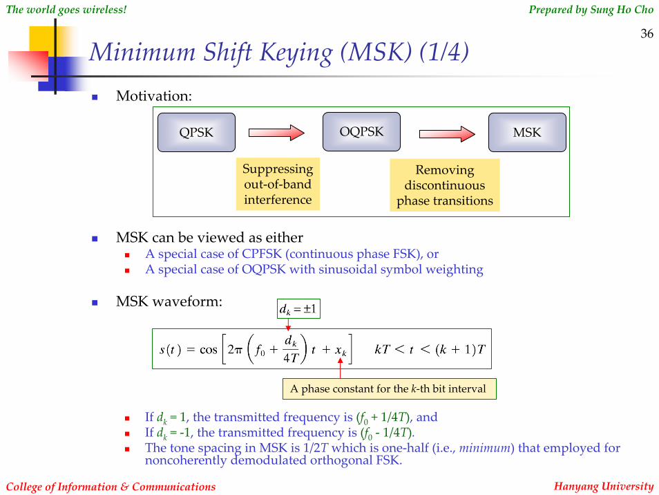
Minimum Shift Keying (MSK) (1/4)Motivation:
MSK can be viewed as eitherA special case of CPFSK (continuous phase FSK), orA special case of OQPSK with sinusoidal symbol weighting
MSK waveform:
If dk = 1, the transmitted frequency is (f0 + 1/4T), and If dk = ‐1, the transmitted frequency is (f0 ‐ 1/4T).The tone spacing in MSK is 1/2Twhich is one‐half (i.e., minimum) that employed for noncoherently demodulated orthogonal FSK.
A phase constant for the k‐th bit interval
QPSK OQPSK MSK
Suppressingout‐of‐bandinterference
Removingdiscontinuous
phase transitions

37
College of Information & Communications
The world goes wireless! Prepared by Sung Ho Cho
Hanyang University
Minimum Shift Keying (MSK) (2/4)Phase constant:
During each T, the value of xk is constant, i.e., xk = 0 or π.The value for xk is determined by the requirement that the phase of the waveform be continuous at t=kT (i.e., continuous phase constraint).
Based on the continuous phase constraint, the MSK waveform can be rewritten as
The ak term can change value only at the zero‐crossing of cos(πt/2T).The bk term can change value only at the zero‐crossing of sin(πt/2T).Thus, the symbol weighting in either the I‐ or Q‐channel is a half‐cycle sinusoidal pulse during 2T seconds with alternating sign.
When viewed as a special case of OQPSK, the MSK waveform becomes
Sinusoidal symbol weighting
ak = ±1bk = ±1

38
College of Information & Communications
The world goes wireless! Prepared by Sung Ho Cho
Hanyang University
Minimum Shift Keying (MSK) (3/4)
MSK as a special case of OQPSK:
Modified I bit stream
I bit stream times carrier
Q bit stream times carrier
Modified Q bit stream
MSK waveform

39
College of Information & Communications
The world goes wireless! Prepared by Sung Ho Cho
Hanyang University
Minimum Shift Keying (MSK) (3/4)
Properties of MSK:The waveform s(t) has constant envelope.There is phase continuity in the RF carrier at the bit transition.The waveform s(t) can be regarded as an FSK waveform with signaling frequencies (f0 + 1/4T) and (f0 ‐ 1/4T).The minimum tone separation is 1/2Twhich is equal to half the bit rate.

40
College of Information & Communications
The world goes wireless! Prepared by Sung Ho Cho
Hanyang University
Power Spectral Densities for QPSK, OQPSK, and MSK
Average power of s(t), P=1 watt

41
College of Information & Communications
The world goes wireless! Prepared by Sung Ho Cho
Hanyang University
Quadrature Amplitude Modulation (QAM) (1/3)
QAM can be viewed as a combination of ASK and PSK.
A simple channel model for QAM:The signal point coordinate (x, y) are transmitted over separate channel, and independently perturbed by Gaussian noise variables (nx, ny), each with zero mean and variance N.
Signal space for M=16 Canonical QAM modulator QAM channel model
42
College of Information & Communications
The world goes wireless! Prepared by Sung Ho Cho
Hanyang University
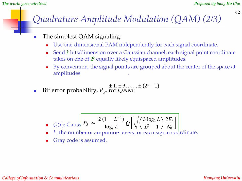
Quadrature Amplitude Modulation (QAM) (2/3)
The simplest QAM signaling:Use one‐dimensional PAM independently for each signal coordinate.Send k bits/dimension over a Gaussian channel, each signal point coordinate takes on one of 2k equally likely equispaced amplitudes.By convention, the signal points are grouped about the center of the space at amplitudes .
Bit error probability, PB, for QAM:
Q(x): Gaussian Q‐functionL: the number of amplitude levels for each signal coordinate.Gray code is assumed.

43
College of Information & Communications
The world goes wireless! Prepared by Sung Ho Cho
Hanyang University
Quadrature Amplitude Modulation (QAM) (3/3)
Bandwidth‐power tradeoff of QAM:
Bandwidth efficiency:
QAM represents a method of reducing the bandwidth required for the transmission of digital data.
In QAM, a much more efficient exchangebetween R/W and Eb/N0 is possible than in MPSK.

44
College of Information & Communications
The world goes wireless! Prepared by Sung Ho Cho
Hanyang University
Waveform Design Example of QAM
Given the design parameters,Data rate: R = 144 Mbits/sAllowable DSB bandwidth = 36 MHz
Q1: Which modulation scheme would you choose?
Required spectral efficiency:
Since 16‐ary QAM requires a lower Eb/N0than 16‐ary PSK, we choose 16‐ary QAM.
Q2: If the available Eb/N0 = 20, what would be the resulting PB?
L = 4
M = 16

45
College of Information & Communications
The world goes wireless! Prepared by Sung Ho Cho
Hanyang University
9. Modulation and Coding for Band‐limited Channels
46
College of Information & Communications
The world goes wireless! Prepared by Sung Ho Cho
Hanyang University
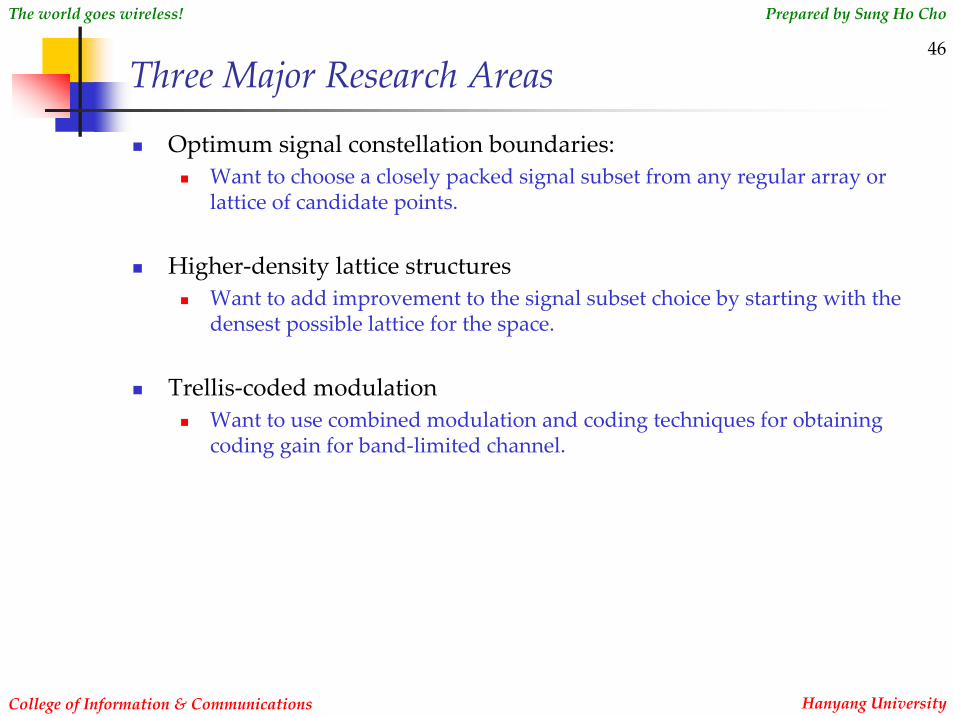
Three Major Research Areas
Optimum signal constellation boundaries:Want to choose a closely packed signal subset from any regular array or lattice of candidate points.
Higher‐density lattice structuresWant to add improvement to the signal subset choice by starting with the densest possible lattice for the space.
Trellis‐coded modulationWant to use combined modulation and coding techniques for obtaining coding gain for band‐limited channel.

47
College of Information & Communications
The world goes wireless! Prepared by Sung Ho Cho
Hanyang University
Commercial Telephone Modems (1/2)
A typical telephone channel:High SNR of approximately 30 dBBandwidth of approximately 3 KHz
Evolution of leased‐line telephone modems:

48
College of Information & Communications
The world goes wireless! Prepared by Sung Ho Cho
Hanyang University
Commercial Telephone Modems (1/2)
Evolution of dial‐line Telephone modem standards:

49
College of Information & Communications
The world goes wireless! Prepared by Sung Ho Cho
Hanyang University
Signal Constellation Boundaries (1/2)
A large number of possible QAM signal constellations have been examined in a search for a designs that result in the best error performance for a given average signal‐to‐noise ratio.
Campopiano‐Glazer constellation construction rule:From an infinite array of points closely packed in a regular array or lattice, select a closely packed subset of 2k points as a signal constellation in a way that the average or peak power of the set is minimized for a given error probability.
M = 4
M = 8
M = 16

50
College of Information & Communications
The world goes wireless! Prepared by Sung Ho Cho
Hanyang University
Signal Constellation Boundaries (2/2)In a two‐dimensional signal space, the optimum boundary surrounding an array of points tends toward a circle.
Examples of 64‐ary (k=6) and 128‐ary (k=7) signal sets from a rectangular array.
The cross‐shaped boundaries are a compromise to the optimum circle.

51
College of Information & Communications
The world goes wireless! Prepared by Sung Ho Cho
Hanyang University
Higher‐Dimensional Signal ConstellationSignaling in a two‐dimensional space can provide the same error performance with less average (or peak) power than signaling in a one‐dimensional PAM space.
We choose points on a two‐dimensional lattice from within a circular rather than a rectangular boundary.
Further energy savings are possible by going to a higher number, N dimensions, and choosing points on an N‐dimensional lattice from within an N‐sphere rather than an N‐cube.
Such reduction in required energy for a given error performance is referred to as a shaping gain.
Energy savings from N‐sphere mapping vs. N‐cube mapping (i.e., shaping gain):
∞ 1.53

52
College of Information & Communications
The world goes wireless! Prepared by Sung Ho Cho
Hanyang University
High‐Density Lattice Structure
We want the densest possible lattice in the space.In a two‐dimensional signal space, the densest lattice is the hexagonal lattice.Examples of hexagonal packing:
Energy savings from the dense lattices vs. the rectangular lattice:

53
College of Information & Communications
The world goes wireless! Prepared by Sung Ho Cho
Hanyang University
Combined Gain: N‐Sphere Mapping and Dense Lattice
The combined energy savings from N‐sphere mapping and dense lattices vs. N‐cube mapping and rectangular lattices: