Modular Invariants for Manifolds with Boundary
80
Modular Invariants for Manifolds with Boundary Maria Immaculada G´ alvez Carrillo
Transcript of Modular Invariants for Manifolds with Boundary

Modular Invariants forManifolds with Boundary
Maria Immaculada Galvez Carrillo

ii

Modular Invariants for Manifolds with Boundary
Memoria presentada per aspirar al grau
de Doctor en Ciencies Matematiques
Departament de Matematiques
Universitat Autonoma de Barcelona
Bellaterra, abril de 2001

iv

Certifico que aquesta memoria ha estat realitzada
per Maria Immaculada Galvez Carrillo i super-
visada per mi, al Departament de Matematiques
de la Universitat Autonoma de Barcelona
Carles Casacuberta Verges
Bellaterra, 27 d’abril de 2001

vi

Summary
This thesis has had two aims: the practical aim of writing out explicit generalisations of the
constructions of Atiyah, Donnelly, Patodi, and Singer [APS75I, APS75II, APS76, ADS84]
for formal sums of operators on manifolds, and the more philosophical aim of re-opening
the investigations of Hirzebruch and Zagier [Hir66, HZ74] on some important interactions of
algebraic topology with number theory and algebraic geometry. We have needed also ingredi-
ents from differential geometry and from analysis, and our investigations led to consideration
of ideas of Segal on conformal field theory [Seg88].
In particular our definitions lead to a new invariant ηE(q) of framed manifolds N4k−1,
which arises on considering the formal operator given by twisting the classical signature
operator by a certain graded bundle considered by Witten [Wit87] as representing the tangent
bundle of the free loop space on a manifold. In this way we obtain an invariant, taking power
series in the formal variable q as values, whose constant term is the spectral eta invariant
of [ADS84]. The result that this eta invariant coincides with the signature defect (i.e., the
difference ϕL(M,N) − sign(M,N) between the relative L-genus and the signature, for a
closed manifold M4k with ∂M = N), generalises to our new invariant to give
ηE(q) = ϕE(M,N) − signS1
(M,N).
Here signS1
is the S1-equivariant signature on the loop space and ϕE is the (normalised)
elliptic genus of [LS88, Och87]; hence the power series ηE can also be regarded as a modular
function, at least modulo the integers. As an illustrative example we note that there are
framings of the spheres S4k−1 = ∂D4k for which ηE is easily expressed in terms of an Eisenstein
series G∗2k.We consider eta invariants arising not only from twisted signature operators, but also
from the corresponding Dirac operators. Moreover we define equivariant versions of these
invariants, associated to representations of the fundamental group G = π1N of the manifold.
Atiyah–Patodi–Singer give an alternative, more algebraic definition of their equivariant eta
invariant in [APS75II], in terms of the K-theory of N and the classifying space BG. We
also generalise this to give a definition in terms of elliptic cohomology of our modular eta
invariant, inspired by the philosophy that K-theory for loop spaces is elliptic cohomology.
We give examples of this construction for lens spaces and, at least in the case that G is finite
of odd order, show that it takes values in the equivariant elliptic cohomology ring introduced
by Devoto [Dev96b].
vii

viii

Contents
1 Essential tools from differential geometry and Clifford theory 9
1.1 Essential tools from differential geometry . . . . . . . . . . . . . . . . . . . . 9
1.1.1 Differential geometry . . . . . . . . . . . . . . . . . . . . . . . . . . . 9
1.1.2 Parallelisations . . . . . . . . . . . . . . . . . . . . . . . . . . . . . . 15
1.1.3 On connections . . . . . . . . . . . . . . . . . . . . . . . . . . . . . . 19
1.1.4 Invariance theory for metric connections with torsion . . . . . . . . . 20
1.2 Essential tools from Clifford theory . . . . . . . . . . . . . . . . . . . . . . . 21
1.2.1 Clifford algebra and spinor bundles . . . . . . . . . . . . . . . . . . . 21
2 Some tools from algebraic topology 27
2.1 Elliptic genera and cohomology theories . . . . . . . . . . . . . . . . . . . . 27
2.1.1 Classical elliptic genera and level 2 elliptic cohomology . . . . . . . . 28
2.1.2 Modularity . . . . . . . . . . . . . . . . . . . . . . . . . . . . . . . . 30
2.1.3 Elliptic cohomology theories and the Miller character . . . . . . . . . 31
2.1.4 Equivariant elliptic cohomology . . . . . . . . . . . . . . . . . . . . . 33
2.2 Relative cobordism theories and classes . . . . . . . . . . . . . . . . . . . . . 35
2.2.1 Relative characteristic classes . . . . . . . . . . . . . . . . . . . . . . 35
2.2.2 Relative multiplicative sequences . . . . . . . . . . . . . . . . . . . . 37
2.2.3 The relative cobordism description . . . . . . . . . . . . . . . . . . . 38
2.2.4 The case of the disk bundles . . . . . . . . . . . . . . . . . . . . . . . 42
2.2.5 Relative genera on framed manifolds . . . . . . . . . . . . . . . . . . 45
3 The Atiyah–Patodi–Singer theorem, elliptic genera and eta invariants 49
3.1 Essential tools from geometric analysis:
Dirac operators and the index theorem . . . . . . . . . . . . . . . . . . . . . 49
3.1.1 First-order elliptic operators on manifolds
with boundary . . . . . . . . . . . . . . . . . . . . . . . . . . . . . . 49
3.1.2 The Atiyah–Singer index theorem . . . . . . . . . . . . . . . . . . . . 51
3.2 The Atiyah–Patodi–Singer theorem . . . . . . . . . . . . . . . . . . . . . . . 52
3.2.1 The classical APS theorem and the eta invariant . . . . . . . . . . . . 52
3.2.2 Generalisations of Gilkey, Donnelly and Nicolaescu . . . . . . . . . . 54
3.2.3 Eta invariants of twisted Dirac operators . . . . . . . . . . . . . . . . 57
ix
3.2.4 Eta invariants of twisted signature operators . . . . . . . . . . . . . . 59
3.3 Elliptic invariants for framed manifolds . . . . . . . . . . . . . . . . . . . . . 61
3.3.1 Classical eta invariants of framed manifolds . . . . . . . . . . . . . . 61
3.3.2 Modular eta invariants for framed manifolds . . . . . . . . . . . . . . 62
3.3.3 Divided congruences and elliptic genera . . . . . . . . . . . . . . . . . 65
3.4 Equivariant elliptic invariants . . . . . . . . . . . . . . . . . . . . . . . . . . 67
3.5 Some eta invariants for lens spaces . . . . . . . . . . . . . . . . . . . . . . . 71
3.5.1 The definitions . . . . . . . . . . . . . . . . . . . . . . . . . . . . . . 71
3.5.2 The proposition . . . . . . . . . . . . . . . . . . . . . . . . . . . . . . 71
3.5.3 First part of the proof . . . . . . . . . . . . . . . . . . . . . . . . . . 71
3.5.4 The twisted signature complex for D4k and Cp actions . . . . . . . . 72
3.5.5 Conclusion of the proof . . . . . . . . . . . . . . . . . . . . . . . . . . 74
3.6 Consequences . . . . . . . . . . . . . . . . . . . . . . . . . . . . . . . . . . . 75
3.6.1 Eta invariants on lens spaces and number theory . . . . . . . . . . . . 75
3.6.2 Multiple elliptic Dedekind sums of level 2 . . . . . . . . . . . . . . . . 80
3.6.3 On topological proofs of reciprocity theorems
for elliptic Dedekind sums . . . . . . . . . . . . . . . . . . . . . . . . 81
4 An algebraic Atiyah–Patodi–Singer construction in elliptic cohomology 83
4.1 E∗-theory with / coefficients . . . . . . . . . . . . . . . . . . . . . . . . 84
4.2 The algebraic extension to elliptic cohomology . . . . . . . . . . . . . . . . . 89
4.3 Geometric interpretation. Modularity of
cohomological eta invariants . . . . . . . . . . . . . . . . . . . . . . . . . . . 91
4.3.1 Virasoro algebras and finite groups . . . . . . . . . . . . . . . . . . . 92
4.3.2 Construction of some G-elliptic objects on
odd-dimensional manifolds . . . . . . . . . . . . . . . . . . . . . . . . 94
4.4 Modularity of elements in elliptic cohomologies
modulo localised integers . . . . . . . . . . . . . . . . . . . . . . . . . . . . . 98
5 Segal annuli and elliptic cohomology 101
5.1 Segal categories of annuli . . . . . . . . . . . . . . . . . . . . . . . . . . . . . 102
5.1.1 Segal annuli . . . . . . . . . . . . . . . . . . . . . . . . . . . . . . . . 102
5.1.2 The torus, moduli, and composition . . . . . . . . . . . . . . . . . . . 105
5.1.3 Principal G-bundles over Segal annuli . . . . . . . . . . . . . . . . . . 106
5.1.4 Spin structures . . . . . . . . . . . . . . . . . . . . . . . . . . . . . . 110
5.2 Representations of Segal annuli . . . . . . . . . . . . . . . . . . . . . . . . . 113
5.2.1 The conformal group and the Virasoro algebra . . . . . . . . . . . . . 113
5.2.2 The twisted group(Diff+(S1
c ))〈g〉 . . . . . . . . . . . . . . . . . . . . 114
5.2.3 Representations of Segal annuli constructions . . . . . . . . . . . . . 115
5.2.4 Change-of-groups properties . . . . . . . . . . . . . . . . . . . . . . . 115
x

Introduction
Atiyah: Why is the A-genus an integer for spin manifolds?
Singer: You know the answer better than I —why do you ask?
Atiyah: There must be a deeper reason.
In March 1962, Singer suggested a deeper reason: the A-genus is an integer
because it is the index of a Dirac operator. . .
The Index Theorem for Manifolds with Boundary
In this thesis we develop some of the Atiyah–Patodi–Singer constructions for manifolds with
boundary in the context of elliptic genera. At least formally, they will provide a version of the
index theorem for the space of free smooth loops on manifolds with boundary. We consider
mainly the case of twisted signature operators corresponding to level 2 elliptic genera, and
we compute and interpret these in the especially relevant cases of some framed disks and
lens spaces. More general results are possible, which will be developed later.
What can elliptic cohomology tell us for manifolds with boundary? We can expect it
to generalise classical results for manifolds with boundary to their free smooth loop spaces,
following the philosophy that elliptic cohomology may be considered as a sort of K-theory of
loop spaces. In this classical case one uses the Chern character to link K-theory to ordinary
cohomology; between elliptic cohomology and K-theory we have the Miller character also.
Using these tools, we can extend the Atiyah–Patodi–Singer constructions to formal operators
on loop spaces on manifolds with boundary.
Recall that the Atiyah–Singer theorem for manifolds without boundary expresses the
index of an elliptic operator in terms of characteristic numbers. More precisely, if we consider
an elliptic operator D+E on a manifold without boundary X, which may be assumed to be
given by the classical signature operator D+ twisted by some bundle E, then the index
is given by
ind(D+E
)= ch2 (E) · L (X) [X] , (1)
where L (X) is the Hirzebruch characteristic class on the tangent bundle TX and ch2 (E) is
the Chern character of E up to a power of 2.
1

For manifolds with boundary, the seminal work of Atiyah–Patodi–Singer [APS75] showed
that an extra summand, the eta invariant, must be added for formula (1) to hold. The
formula obtained becomes
ind(D+E
)+ dim kerD+
E |Y= ch2 (E) · L (X) [X] − ηD+E |Y (0)
at least in those cases when we consider a compact oriented Riemannian manifold X of
dimension 4k with boundary Y and assume that near Y it is isometric to a product. Here
ηD+E |Y is the holomorphic continuation of the eta function
η (s) =∑λ
sign (λ)
|λ|s , Re (s) 0,
where the sum is over the non-zero eigenvalues of the operator.
Modular Eta Invariants
In this thesis we define and calculate these invariants for formal operators on loop spaces
on manifolds with boundary, and interpret them as modular invariants. In particular, we
consider the formal operator corresponding to the signature for a bundle E,
RqE =
∞⊗j=1
SqjE ⊗∞⊗j=1
ΛqjE,
where SqjE and ΛqjE are the formal power series versions of the symmetric and exterior
products. Then the index theorem applied to this formal operator will give a formal power
series instead of a numerical index. If X is a manifold without boundary and E its complex-
ified tangent bundle, we write ξq = RqE and the index formula becomes
ind(D+ξq
)= Φε (X) [X] .
The characteristic class Φε (X) is precisely determined by the elliptic genus
ϕε : ΩSO∗ −→ E∗ ∼= [12][δ, ε][∆−1],
whose exponential series is given by the elliptic function sε (τ, x) = (℘ (τ, x) − ℘ (τ, πi))−12 .
For any class [X] ∈ ΩSO∗ in the oriented cobordism ring corresponding to a manifold of dimen-
sion 4k, ϕε ([X]) is a modular form of weight 2k for the congruence subgroup Γ0 (2) < SL2.
Once we normalise it by dividing out by the factor ε (τ)k2 it becomes a modular function
for the congruence subgroup Γ0 (2) which coincides with the formal index of the graded
operator D+ξq
,
ind(D+ξq
)=∞∑r=0
ind(D+r
)qr = Φε (X) [X] =
ϕε(X)
ε (τ)k2
,
2

with each of the coefficients in its q-expansion corresponding to the index of a twisted
signature operator of finite rank over X.
If now X has boundary Y , what can we say about the formal sum
ηD+ξq|Y (0) =
∞∑r=0
ηD+r |Y (0)qr (2)
of eta invariants corresponding to the summands of these formal operators? We will show
they also give a class of modular invariants; these are the modular invariants of the title of
this thesis. Term by term application of the Atiyah–Patodi–Singer theorem, combined with
suitable relative versions of elliptic genera, will ensure that the series (2) is well defined, and
converges. In particular, we obtain
ind(D+ξq
)+ dim kerD+
ξq|Y = Φε (X, Y,∇) [X, Y ] − ηD+
ξq|Y (0) ,
using the definitions for graded dimensions as defined for instance in [FLM88]. The relative
characteristic classes introduce rational coefficients and we see, modulo the integers, that
ηD+ξq|Y (0) is always congruent to a modular function of level 2 with rational coefficients.
Furthermore, if the left-hand side vanishes, then ηD+ξq|Y (0) will be a modular function of
level 2 with rational coefficients. In terms of the elliptic genus, we have shown that
ind(D+ξq
)+ dim kerD+
ξq|Y =
ϕε (X, Y,∇)
ε (τ)k2
− ηD+ξq|Y (0) .
Observe that the connection on which the characteristic forms are based appears now
explicitly in the expressions. Unlike the case of manifolds without boundary, on a manifold
with boundary it is possible to have defined two elliptic operators with the same principal
symbol (and hence the same K-theoretic class in the description by Atiyah and Singer),
but different indices. In particular, we will generically obtain different invariants whenever
we consider operators defined using different connections. Even restricting ourselves to the
case of metric-compatible connections for a fixed Riemannian structure on the manifold, the
result obtained will depend on the torsion tensor considered.
This allows more analytical invariants to be obtained than in the case of manifolds without
boundary, corresponding to operators sharing the same principal symbol but not their total
symbol. We will concentrate on the formal operators on loop spaces which extend the
signature-based operator considered by Atiyah, Donnelly and Singer in [ADS83]. The usual
signature operator on differential forms on a Riemannian manifold is determined by the
composite d∇0
= ∧ ∇0 of the Levi-Civita connection ∇0 and the exterior product ∧;
this operator d∇0
agrees with the usual exterior derivative. If instead of the Riemannian
connection we use any other metric connection ∇T with torsion tensor T , we obtain an
operator d∇T
= ∧ ∇T which shares with d∇0
the principal symbol, but which will not have
the same index in general for manifolds with boundary. In fact, the operator considered by
[ADS83] is a particular case of d∇T: if one considers a manifold X with framed boundary
3

(Y, f), the framing determines a flat connection on Y , extending to a connection ∇f on X
compatible with the metric but not necessarily flat. Then, since we fixed the curvature, we
know from Riemannian geometry that it will have some non-vanishing torsion tensor T , such
that ∇f = ∇T , and d∇f
= d∇T.
Using a formal loop version of [ADS83] for this operator, we show that the resulting eta
invariants are the reduction modulo [12] of modular functions of level 2. We compute these
invariants explicitly for the case of the framed disks(D4k, S4k−1, π
)whose stable tangent
bundles generate relative KO-theory coefficients up to the prime 2. These manifolds are
especially interesting for algebraic topology, since they generate the relative oriented cobor-
dism groups ΩSO, fr∗ [1
2] and ΩU, fr
∗ of oriented and unitary manifolds with respect to framings
of their boundaries. Moreover, using the exact sequences
0 → ΩU2n → ΩU, fr
2n → Ωfr2n−1 → 0,
the framed disks were used by Conner and Floyd in [CF66] to determine the image of the
Adams e-invariant by relating the e-invariant to a relative Todd genus
0 → ΩU2n → ΩU, fr
2n → Ωfr2n−1 → 0
↓ TdU ↓ TdU, fr ↓ e
0 → → → / → 0.
The odd part of the image of e is given by the modified Bernoulli numbers, well known to
topologists, which arise as the values of the invariant on the framed disks considered above.
On the other hand, it was proved in the seventies by Atiyah–Patodi–Singer in their original
work [APS75II] that these e-invariants are in fact reduced eta invariants for Dirac operators
on framed manifolds.
Now the elliptic genus that we use is generated by Eisenstein series G∗2k (τ) whose
q-expansions have constant term(1 − 22k−1
)B2k/4k. Noting that the twisted signature
vanishes, we show that the formal loop space signature of these disks has corresponding eta
invariant 4G∗2k(τ)/ε (τ)k, whose q-expansion is indeed the Adams e-invariant in its oriented
version [see Sto68, p. 215]. This result can be seen as a particular case of a more general
statement for Hirzebruch genera determined by formal operators.
Although it is not in the scope of the present thesis, in later work we would like to make
more explicit how L-series, Jacobi forms, Rademacher sums, modular forms of half-integral
weight, and more general Eisenstein series come into the picture. This is an old wish and,
indeed, from Atiyah’s work and commentaries in Hirzebruch’s Collected Papers, one sees
that it arose at the very origin of the subject. It was Hirzebruch who first spotted what
he called the Signaturdefekt on manifolds with cusps and who gave the hint of the role of
number theoretic L-series in this area.
4

Equivariant Elliptic Cohomology
As in the original work [APS75], an important part of our research takes place in the equivari-
ant world. We use the equivariant elliptic cohomology developed by Devoto to construct our
invariants, in the same spirit as they arose from equivariant K-theory in the classical case.
We will summarise our result by the test case of lens spaces L4k−1p obtained as the
quotient of (4k − 1)-dimensional spheres by a cyclic group G = Cp of odd order. We
then have two families of invariants from the classical signature operator: the first gives us
invariants ηAξq(S4k−1), g
for the formal twisted signature operator on LS4k−1 associated to each
g ∈ G, and the second gives invariants ηAξq(L4k−1
p ), α for a formal twisted signature operator
on LL4k−1p associated to a representation α of G. These two families are related via a finite
Fourier transform formula, which classically gives the well-known expressions for the lens
spaces Y = L4k−1p (q1, . . . , q2k) = S4k−1/Cp,
ηε,α (0, Y ) =1
p
p−1∑r=1
2k∏j=1
cot
(πqjr
p
)χα(ζrp)
(compare [APS75II, p. 412], [Don78, Thm. 3.3]). The number-theoretic significance of such
expressions was known already to Rademacher. Our generalisation gives an expression for
the modular eta invariant in terms of the Teilwerte ϕ (τ, 2πiqjr/p) of the chosen elliptic
functions,
ηε,α (0, Y ) =1
p
p−1∑r=1
2k∏j=1
ϕ (τ, 2πiqjr/p)
ε (τ)12
χα(ζrp).
The ϕ (τ, 2πiqjr/p) are modular for the subgroup Γ = Γ1 (p) ∩ Γ0 (2) of SL2 (), and we
see that ηε,α (0, Y ) and ηε,g
(0, Y
)are modular functions for this Γ. We hope to investigate
general “elliptic Rademacher expansions” in later work.
We also introduce algebraic elliptic eta invariants based on elements of Devoto’s equivari-
ant cohomology ring E∗G [Dev96, Dev98]. The definition of these invariants again parallels
that of Atiyah–Patodi–Singer for K-theory, and requires some technical results concerning
elliptic cohomology with coefficients in /[12], which is developed in a section of its own.
To describe our algebraic construction of eta invariants, consider a spin manifold Y of di-
mension 4k − 1, which we may suppose bounds. The invariants in [APS75] associate to a
representation of π1(Y ) an invariant in K∗ (pt;/). We extend this construction, in the
natural way, by giving invariants in the appropriate version of elliptic cohomology.
Next, we use the result of [HKR00, Dev96b] that for a finite group G of odd order there
is a completion map cG which is an isomorphism,
E∗ (BG) ⊗ [
1|G|
] cG∼= (E∗G)∧IG,
for IG the kernel of the augmentation map
ε : E∗G → E∗e ⊗ [
1|G|
].
5

We apply this to replace E∗G by E[
1|G|
]∗BG and use the connecting map of the short
exact sequence of coefficient groups
0 → [12] → → /[1
2] → 0
to establish an isomorphism
E[
1|G|
] even
(BG) ∼= E odd
/[12](BG) .
We will use this isomorphism to get invariants on manifolds as follows. Consider a
(4k − 1)-dimensional manifold Y with spin structure, which we may assume bounds a man-
ifold X, whose fundamental group π1(Y ) = G is finite of odd order. For the corresponding
classifying map f : Y → BG its pullback f ∗ : E odd/[ 1
2](BG) → E odd
/[ 12](Y ) gives classes in
the elliptic cohomology of the manifold itself. Using the appropriate suitable Gysin map,
any such class will give us an element in E odd/[ 1
2](pt). This is where our invariants live, and
so we have extended the [APS75] definition to the framework of elliptic cohomology.
We can develop this construction for the test case of lens spaces, explicitly compute the
invariants, and verify that they correspond to the ones given above for equivariant formal
signature operators for loop spaces.
A key point in the construction is the mod [12] reduction of the invariants. Since
/, /[12] or p/p are not even rings, it does not immediately make sense to consider
“modular forms with coefficients mod ”, or “p-adic modular forms with coefficients mod
p”. Nevertheless, at this point, the work of Katz [Kat75] and its applications by Baker,
Clarke, Laures and others is relevant, as well as the description by Hopkins. After defining
elliptic cohomology with rational coefficients modulo some ring of localised integers, we can
split the coefficient group /, at least for the case of finite-dimensional manifolds (and in
particular for the point) as the direct sum of coefficient rings of the form E∗ ⊗ /(p∞),
p an odd prime, so that any ring of the form E∗⊗/(pk) will be in the coefficients. More-
over, our aim is to see how this amounts to considering together all the congruences between
modular forms —in our case for Γ0 (2)— modulo pk, which hold for every k, for p a fixed odd
prime. This puts us in the setting of the Katz divided congruence rings and p-adic modular
forms. We will only outline these results, and describe briefly how it is a particular case of
a more general construction related to the generalised character constructions of [HKR00].
Representations of Segal Annuli
Finally we consider our constructions and their invariants in the light of conformal field
theory proposed in the widely circulated preprint of Graeme Segal [Seg88]. To fill in all the
details is beyond the scope of this thesis, but we will recall some particular constructions
which play a natural role in our theory. We introduce the Segal category ASpin (G) of G-Segal
annuli with spin structure and consider their representation theory; in particular we study
6

the functoriality, Mackey and Green properties of the functor which associates to each G the
set of representations of the corresponding ASpin (G). Identification of these representations
and their graded characters allows us to define an equivariant version of the result relating
the Segal annuli A and the space (0, 1)×Diff+(S1)×Diff+(S1)/S1. The Lie algebra Vect (S1)
of fields over S1 and its extension, the Virasoro algebra, now enter the picture. Our intention
is then to define certain natural representations ρΘg of an equivariant generalisation VirG, Spin
of the Virasoro algebra, from whose graded characters we recover our elliptic invariants of
the previous chapters.
There is a clear relation of these representations with the elliptic objects of Baker and
Thomas [BT89] (also motivated by Devoto’s work) which parallels the classical relation
between representation theory, equivariant bundle and K-theory, and the cohomology of the
classifying spaces of finite groups.
7

8

Chapter 1
Essential tools from differential
geometry and Clifford theory
The goal of this chapter is to set up the frame where we are going to work, to fix notation,
and to recall the classical results —mainly from differential geometry, geometrical analysis,
and algebraic topology— which are going to be used. In particular, we will need to use
the properties of connections with torsion, bundles graded by formal variables, and spinor
bundles on spheres.
1.1 Essential tools from differential geometry
In this section we set up the notation for the tools from differential geometry that we will
need. We will work mainly with smooth manifolds with boundary, equipped with a fixed
Riemannian metric. We consider affine linear connections on bundles naturally obtained
from the tangent bundle of these manifolds, usually compatible with the metric, but not
necessarily the Levi-Civita connection, since we allow torsion. We give the definitions for
the operators from Riemannian geometry adapted to the case of non-vanishing torsion, and
we make explicit some expansions in terms of coordinates and moving frames very usual
in the Levi-Civita case, but less known in the presence of non-zero torsion. Then we will
introduce Tamanoi’s generalised differential forms and we will identify the metric and the
torsion. We will identify the essential generalised differential parallel forms.
1.1.1 Differential geometry
We briefly review a number of important concepts and definitions of differential and Rie-
mannian geometry, several of which will be needed in greater generality in later sections of
this thesis.
9

Manifolds, connections, tensor fields and forms
Let Mn be an n-dimensional smooth manifold. If π : E → M is a vector bundle over M ,
we write Γ(M,E) or just ΓE for the space of global smooth sections s of E. If we take the
tangent bundle E = TM or cotangent bundle E = T ∗M = TM∗, given in each coordinate
neighbourhood (U, x) by
⟨∂
∂x1, . . . ,
∂
∂xn
⟩or 〈dx1, . . . , dxn〉, then ΓE is the space of vector
fields or of 1-forms on M respectively.
The space of vector fields acts on the space C∞(M) = C∞(M,) of smooth scalar
functions on M ,
C∞(M) ⊗ ΓTM → C∞(M)
f ⊗X → X(f).
If X is given in local coordinates by∑ai∂
∂xithen X(f) is defined by
∑ai∂f
∂xi. Vector fields
may be identified with endomorphisms X of C∞(M) which satisfy the Leibniz rule,
X(f · g) = X(f) · g + f ·X(g).
The space of vector fields forms a Lie algebra with bracket
[X, Y ](f) = X(Y (f)) − Y (X(f)).
A connection on a vector bundle E → M is a linear map
∇ : ΓE → Γ(TM∗ ⊗ E)
satisfying a Leibniz rule
∇(fs) = f∇s+ df ⊗ s
where the total derivative df is the 1-form defined by (df)(X) = X(f) or, in local coordinates,
by∑ ∂f
∂xidxi. Since elements of ΓTM∗ may be evaluated at X ∈ ΓTM , one has covariant
derivatives of sections of E along vector fields:
ΓE ⊗ ΓTM → ΓE
s⊗X → ∇Xs,
satisfying ∇X(fs) = f∇Xs+X(f)s and ∇fXs = f∇Xs.
If the vector bundle E is equipped with a metric g(−,−) = 〈−,−〉, then a connection ∇on E is compatible with the metric if for all sections s, t ∈ ΓE and vector fields X one has
X〈s, t〉 = 〈∇Xs, t〉 + 〈s,∇Xt〉.
A connection on M is a connection on the tangent bundle TM .
10
We denote by SkE, ΛkE and E⊗k the symmetric, exterior and tensor product bundles of
a vector bundle E. A (k, )-tensor field is a section of (TM∗)⊗k ⊗ TM⊗, and a differential
k-form is a section of ΛkTM∗. Given a connection ∇ on M , the covariant derivatives
∇X : ΓTM → ΓTM on vector fields Y may be extended to act on 1-forms ω and (inductively)
on arbitrary (k, )-tensor fields via the following dual and tensor product formulas
X(ω(Y )) = (∇Xω)(Y ) + ω(∇XY ),
∇X(P ⊗Q) = ∇XP ⊗Q + P ⊗ ∇XQ.
Allowing X to vary, one has for any (k, )-tensor field P a (k + 1, )-tensor ∇P defined by
(∇P )(Y ⊗X ⊗ ϕ) = (∇XP )(Y ⊗ ϕ)
= X(P (Y ⊗ ϕ)) −k∑i=1
P (Y1 ⊗ · · · ⊗ ∇XYi ⊗ · · · ⊗ Yk ⊗ ϕ)
+
∑j=1
P (Y ⊗ ϕ1 ⊗ · · · ⊗ ∇Xϕj ⊗ · · · ⊗ ϕ),
for Y = Y1 ⊗ · · · ⊗ Yk ∈ ΓTM⊗k and ϕ = ϕ1 ⊗ · · · ⊗ ϕ ∈ Γ(TM∗)⊗.
Examples 1.1
1. The condition for the connection to be compatible with a metric may be expressed
as ∇g = 0.
2. For a “(0, 0)-tensor” f ∈ C∞(M) we have (∇f)(X) = ∇Xf = X(f), and ∇f coincides
with the total derivative df .
3. For a p-form ϕ we have a (p + 1, 0)-tensor ∇ϕ. Antisymmetrising this tensor gives a
(p+ 1)-form (∧ ∇)ϕ which satisfies
(∧ ∇)ϕ(X0, . . . , Xp) =1
p+ 1
(∑i
(−1)iXi(ϕ(X0, . . . , Xi, . . . , Xp)) +
+∑i<j
(−1)i+jϕ(∇XiXj − ∇Xj
Xi, X0, . . . , Xi, . . . , Xj, . . . , Xp)
).
Definition 1.2 A natural vector bundle over a manifold M is a vector bundle which may
be constructed from the tangent bundle TM by taking direct sums, tensor products, duals,
and symmetric and exterior products.
11

Any connection on M extends as above to a connection on any natural bundle over M . Since
all the bundles considered in this thesis will be natural bundles, we will often forget the word
“natural”.
We write ΩkM = ΓΛkTM∗ for the space of k-forms and, more generally, we write
Ωk(M ;E) = Γ(ΛkTM∗ ⊗ E). The space
Ω∗M =⊕
ΩkM
of all forms on M is a graded-commutative algebra with respect to ∧, with ΩkM = 0 for
k > n. The pairing between vector fields and 1-forms extends to interior multiplication maps
i(X) : Ωk+1M → ΩkM for X ∈ ΓTM , defined inductively by
i(X)(ω1 ∧ · · · ∧ ωk) = ω1(X)ω2 ∧ · · · ∧ ωk − ω1 ∧ i(X)(ω2 ∧ · · · ∧ ωk).
The exterior derivative d : Ω∗M → Ω∗+1M is the unique linear map extending the total
derivative C∞(M) → ΓTM∗, f → df , and satisfying d(fϕ) = (df) ∧ ϕ. If dϕ = 0, then ϕ
is a closed form. The covariant exterior derivative d∇∗ : Ω∗(M ;E) → Ω∗+1(M ;E) associated
to a connection ∇ : ΓE → Γ(TM∗⊗E) is the unique linear map extending ∇ and satisfying
d∇p (ϕ⊗ s) = dϕ⊗ s+ (−1)pϕ ∧ d∇s.
C∞(M) dΩ1M d
Ω2M · · · ΩkM dΩk+1M · · ·
ΓE ∇Ω1(M ;E) d∇
Ω2(M ;E) · · · Ωk(M ;E) d∇Ωk+1(M ;E) · · ·
The exterior derivative satisfies d2 = 0 and the cohomology of the complex (Ω∗M, d) is
the de Rham cohomology of M , which is isomorphic to the real singular cohomology of M .
The map d∇ ∇ : ΓE → Ω2(M ;E) is not always zero; when it is, the connection ∇ is termed
flat. The curvature tensor R of the connection may be defined by 2R = d∇∇ or, evaluating
on a pair of vector fields X, Y ∈ ΓTM , by
RX,Y (s) = ∇X(∇Y s) − ∇Y (∇Xs) − ∇[X,Y ]s.
Riemannian manifolds, metrics and torsion
Consider now the special case of the tangent bundle E = TM , although our remarks will all
carry over to any natural bundle E. The curvature tensor for a connection
∇ : ΓTM → Γ(TM∗ ⊗ TM)
on M may be regarded as a (3, 1)-tensor on M . It satisfies the Bianchi identities
RX,Y Z − T (T (X, Y ), Z) − (∇XT )(Y, Z) = 0
(∇XR)Y,Z +RT (X,Y ),Z = 0
12

where the notation P (X, Y, Z) = P (X, Y, Z)+P (Z,X, Y )+P (Y, Z,X) refers to the cyclic
sum of a (3,−)-tensor, and T is the torsion tensor associated to the connection ∇ on M ,
i.e., the (2, 1)-tensor defined by
T (X, Y ) = ∇XY − ∇YX − [X, Y ].
If T = 0 then the connection is termed torsion-free (or symmetric), and the Bianchi identities
become RX,Y Z = (∇XR)Y,Z = 0. From Example 1.1.3 one sees also that ∧∇ coincides
with d : ΩpM → Ωp+1 if ∇ is torsion-free.
If the tangent bundle of M is equipped with a metric 〈 , 〉 then (M, 〈 , 〉) is termed a
Riemannian manifold.
Proposition 1.3 On a Riemannian manifold there is a unique connection which is both
compatible with the metric and torsion-free, termed the Levi-Civita or canonical Riemannian
connection.
In this case the corresponding (Riemannian) curvature tensor is completely determined by
the sectional curvature,
K(X ∧ Y ) = 〈RX,Y Y,X〉 / (|X|2|Y |2 − 〈X, Y 〉2).
In fact any connection ∇ on M which is compatible with the Riemannian metric is
determined by its torsion tensor T . Explicitly, one finds that
2 〈∇XY, Z〉 = X〈Y, Z〉 + Y 〈Z,X〉 − Z〈X, Y 〉 − 〈X, [Y, Z]〉 + 〈Y, [Z,X]〉+ 〈Z, [X, Y ]〉 − 〈X, T (Y, Z)〉 + 〈Y, T (Z,X)〉 + 〈Z, T (X, Y )〉. (1.1)
Definition 1.4 We will denote by ∇g,T the connection on M that is uniquely determined
by (1.1), which has torsion given by the antisymmetric tensor T and is compatible with a
metric g = 〈 , 〉.Taking T = 0 in equation (1.1) gives an expression for the Levi-Civita connection ∇ = ∇g,0
on M , and also for the exterior derivative, since d = ∧ ∇ in the torsion-free case.
Oriented manifolds, the Hodge star and coderivatives
A (connected) n-dimensional Riemannian manifold M is orientable if the double cover Or
of M , with fibres given by the orthonormal frames in TM modulo the action of SOn, is just
the trivial double cover M ∪M . In the language of algebraic topology, M is orientable if the
first Stiefel–Whitney class w1 ∈ H1(X;2) vanishes, where w1 may be thought of as classi-
fying the double cover Or via the isomorphism H1(X;2) ∼= Hom(π1X,2). An orientation
on M is then a choice of one sheet of the double cover.
Alternatively, an orientation on M is a nowhere-vanishing global n-form Φ ∈ ΓΛTM∗.Two such orientations Φ1,Φ2 are equivalent if Φ1 = fΦ2 for some everywhere-positive func-
tion f ∈ C∞(M), or opposite if f is everywhere negative. The volume form of a manifold
13

with orientation Φ is given by the normalisation
dv =Φ
|Φ|√n!.
The Hodge star operator for an oriented Riemannian manifold is the linear isomorphism
∗ : ΩqM −→ Ωn−qM
ω1 ∧ · · · ∧ ωq → ωq+1 ∧ · · · ∧ ωn,
where (ω1, . . . , ωn) is any (positive) orthonormal coframe of 1-forms, so that in particular
dv = ω1 ∧ · · · ∧ ωn = ∗1.
For q-forms ϕ, ψ one has
ϕ ∧ ∗ψ = 〈ϕ, ψ〉dv, ∗(∗ϕ) = (−1)q(n−q)ϕ.
If M is compact, one defines the inner product and L2-norm on ΩqM by
(ϕ, ψ) =
∫M
〈ϕ, ψ〉dv, ‖ϕ‖2 = (ϕ, ϕ).
The exterior coderivative δ : ΩqM → Ωq−1M is then the adjoint of d under the L2-norm,∫M
〈φ, δϕ〉dv =
∫M
〈dφ, ϕ〉dv.
A differential form ϕ is called harmonic if ∆ϕ = 0, where ∆ is the Laplace operator
∆: ΩqM → ΩqM ,
∆ = (d+ δ)2 = dδ + δd.
Since (∆ϕ, ϕ) = ‖dϕ‖2 + ‖δϕ‖2, we see that ϕ is harmonic if and only if both dϕ and
δϕ vanish. Let ϕ be any closed q-form. Then Hodge’s theorem on critical points of the
L2-norm implies that there exists a unique (q − 1)-form φ such that δ(ϕ+ dφ) = 0 (in fact,
minimising ‖ϕ+ dφ‖2), and so ϕ+ dφ is the unique harmonic form in the cohomology class
of ϕ. The de Rham cohomology groups of a compact oriented Riemann manifold M are
therefore isomorphic to the spaces of harmonic forms on M .
Proposition 1.5 The exterior coderivative δ on forms on an oriented, compact Riemannian
manifold without boundary can be expressed in terms of d and the Hodge star,
δ = (−1)(q−1)(n−q+1)+q ∗d∗ : Ωq(M) −→ Ωq−1(M).
Proof: Integration over M of the form
d(φ ∧ ∗ϕ) = dφ ∧ ∗ϕ+ (−1)q−1φ ∧ d∗ϕand application of Stokes’ formula shows that we can take ∗δϕ = (−1)qd∗ϕ.
In particular the Hodge star of a harmonic form is again harmonic and induces isomorphisms
∗ : Hq(M) ∼= Hn−q(M).
14

1.1.2 Parallelisations
This is essential for framed manifolds and connections on them. A parallelisation of a
smooth n-dimensional manifold M is a section of the bundle LM of n-frames on the tangent
bundle TM .
As we next make precise, every parallelisation determines a metric and a connection that
is compatible with the metric (since the size of vectors is unaltered by parallel transport).
This connection need not be symmetric. For our exposition we follow an approach by Dodson.
Theorem 1.6 Suppose that an n-dimensional manifold M is parallelisable by a section
p: M −→ LM
x −→ (pi)x .
Then p determines a connection ∇p in LM such that
∇ppi
(pj) = 0 for all i, j = 1, . . . , n.
If h : M → GL (n;), x → [hij]x, is a smooth map, then qi = hki pk defines another paralleli-
sation, and ∇p = ∇q if and only if h is constant on each connected component of M .
Proof: By hypothesis, the Christoffel symbols for ∇p with respect to the frame (pi)x all
vanish, since
∇ppi
(pj) = Γkij pk.
Locally, the splitting of TuLM for u =(x,(bijpi
)x
)∈ LM is given as TuLM = Hu ⊕Gu by(
x,(bijpi
)x, X,B
)=(x,(bijpi
)x, X, 0
)⊕(x,(bijpi
)x, 0, B
). We choose
Hp(x) = Dxp (TxM)
and for any u ∈ LM , with u = Rh (p (x)),
Hu = Dp(x)Rh
(Hp(x)
).
By the existence of p, we know that
LM = M × GL (n;)
and the connection ∇p makes the horizontal subspaces look horizontal in this product bun-
dle by
LM → M ×G(x,(bijpi
)x
) −→
(x,(δij)x
).
15

That is, we locate the identity in G at the frame determined by the parallelisation at each
point.
The given q is another parallelisation and
∇ppi
(qj) = ∇ppi
(hkjpk
)= pi
(hkj)pk + hjk∇p
pipk,
and ∇ppi
(qj) = 0 if and only if hkj is constant on each connected component of M .
Corollary 1.7 The connection ∇p need not be symmetric.
Corollary 1.8 The geodesics of ∇p are the integral curves of constant linear combinations
like X : M → TM , x → aipi.
Example: a nontrivial parallelisation of the plane
A nontrivial parallelisation of the two-plane 2 is given by
p: 2 −→ L2
(x, y) −→ (ex∂1, ex∂2) ,
with ∂1 =∂
∂xand ∂2 =
∂
∂ygiving the standard frame of T(x,y)2 via the identity chart on 2 .
This p is a parallelisation and it determines a connection ∇p by the conditions, since ex is
never zero, and hence, by linearity of ∇pvw in v,
∇p∂i
(ex∂j) = 0 for i, j = 1, 2,
which expands to
ex∂j + exΓp.∂,k1,j ∂k = 0 for i = 1,
exΓ∂,k2,j ∂k = 0 for i = 2.
It follows that [Γp,∂,1i,j
]=
[ −1 0
0 0
],[Γp,∂,2i,j
]=
[0 −1
0 0
],
and obviously ∇p fails to be symmetric because
Γ212 = Γ2
21.
Moreover, p determines a Riemannian structure gp which, in standard coordinates (i.e.,
the ∂-basis), gives [gp,∂i,j
]=
[e−2x 0
0 e−2x
].
16

The Ricci Lemma may be used to see that ∇p is compatible with gp. It amounts to check
the compatibility equation
u (gp (v, w)) = gp (∇puv, w) + gp (v,∇p
uw)
for all tangent vector fields u, v, w. In the component form u = ∂i, v = ∂j , w = ∂k, the
left-hand side is [∂1g
p,∂i,j
]=
[ −2e−2x 0
0 −2e−2x
][∂2g
p,∂i,j
]=
[0 0
0 0
],
while the right-hand side is
gp(Γp,∂,mki ∂m, ∂j
)+ gp
(∂i,Γ
p,∂,mkj ∂m
)= gp,∂
m,jΓp,∂,mki + gp,∂
m,iΓp,∂,mkj
= e−2xΓp,∂,jki + e−2xΓp,∂,i
kj
and since [Γp,∂,j
1,i
]=
[ −1 0
0 −1
],[Γp,∂,j
2,i
]=
[0 0
0 0
],[
Γp,∂,i1,j
]=
[ −1 0
0 −1
],[Γp,∂,i
2,j
]=
[0 0
0 0
],
we see then that ∇p is indeed compatible with gp. However, since it is not symmetric, it is
not the Levi-Civita connection of any metric tensor field. In fact, the Levi-Civita connection
∇gp determined by the parallelisation metric gp can be found by solving the equation of the
Ricci Lemma. In coordinates, one has that its components Γgp,∂,k
i,j satisfy
∇gp
∂i∂j = Γ
gp,∂,k
i,j ∂k, by definition, and
gp,∂k,mΓg
p,∂,kij =
1
2
(∂ig
p,∂j,m + ∂jg
p,∂i,m − ∂mg
p,∂i,j
), by the Ricci Lemma,
so that [Γg
p,∂,1i,j
]=
[ −1 0
0 1
],[Γg
p,∂,2i,j
]=
[0 −1
−1 0
],
with compatibility [Γg
p,∂,j1,i
]=
[ −1 0
0 −1
],[Γg
p,∂,i2,j
]=
[0 −1
1 0
],[
Γgp,∂,i
1,j
]=
[ −1 0
0 −1
],[Γg
p,∂,i2,j
]=
[0 1
−1 0
],
so that, for k = 1, 2,
∂kgp,∂i,j = e−2x
(Γg
p,∂,jk,i + Γg
p,∂,ik,j
).
17

Jet bundles and stable jet bundles
Let (M, g) be a Riemannian manifold of dimension m, and identify TM and T ∗M through g.
For a vector bundle E over M , define the jet bundle
J (E) = E ⊕ (E ⊗ TM)
and the iterated jet bundles
J i (E) = J(J i−1 (E)
).
Likewise, define the stable jet bundle
(J (E))s = 1 ⊕ J (E) = 1 ⊕ E ⊕ (E ⊗ TM)
and the iterated stable jet bundles(J i (E)
)s= 1 ⊕ J i (E) = 1 ⊕ J
(J i−1 (E)
).
Remark that
(J (E))s = 1 ⊕ E ⊕ (E ⊗ TM)
∼= 1 ⊕ (E ⊗ 1) ⊕ (E ⊗ TM)
∼= 1 ⊕ E ⊗ (1 ⊕ TM)
∼= 1 ⊕ E ⊗ T sM,
where T sM is the stable tangent bundle of M . In that formalism,
(J (E))s = 1 ⊕ (E ⊗ T sM)(J2 (E)
)s= 1 ⊕ (J (E) ⊗ T sM) = 1 ⊕ (E ⊗ T sM⊗2
)(J3 (E)
)s= 1 ⊕ (J2 (E) ⊗ T sM
)= 1 ⊕ (E ⊗ T sM⊗3
)· · ·(
J i (E))s
= 1 ⊕ (J i−1 (E) ⊗ T sM)
= 1 ⊕ (E ⊗ T sM⊗i),
and in particular
J i (M) = J i (TM) = 1 ⊕(TM ⊗ (1 ⊕ TM)⊗i
).
A vector bundle E is said to be flat if it admits a connection whose curvature vanishes
identically. Vector bundles can admit inequivalent flat structures. A manifold M is said to
be flat if TM is flat, and M is called i-th order flat if J i (M) admits a flat structure. We
denote by α (M) the smallest integer i for which J i (M) admits a flat structure; otherwise,
α (M) = ∞. If J i (M) admits a flat structure for some i, then the rational Pontrjagin classes
of M are zero in positive degrees and TM is rationally trivial. For n > 1, J i ( Pn) is never
flat, so that, if n > 1, α ( Pn) = ∞.
For the sphere Sn, one has J (Sn) = J1 (Sn) = T (Sn) ⊗ (1 ⊕ T (Sn)).
18

1.1.3 On connections
We will consider a linear connection on a bundle ξ over a compact smooth manifold M with
boundary, as a map
∇ : Γ (M, ξ) → Γ (M,T ∗M ⊗ ξ) .
A linear connection ∇ on a manifold provides a covariant way to differentiate tensor fields.
It provides a type-preserving derivation on the algebra of tensor fields that commutes with
contractions. Given an arbitrary local basis of vector fields Xa, the most general linear
connection is specified locally by a set of n2 1-forms ωab where n is the dimension of the
manifold,
∇XaXb = ωcb(Xa)Xc.
Generally, we will be given a metric on the manifold and we will restrict ourselves to metric-
compatible connections. However, we do not ask our connection to be torsion-free. In partic-
ular, we will deal mainly with connections on bundles constructed from the tangent bundle
of the manifold.
So, for our connections, the following will hold in general, for fields X, Y, Z:
X(g(Y, Z)) = S(X, Y, Z) + g(∇XY, Z) + g(Y,∇
XZ),
but
T (X, Y ) = ∇XY − ∇
YX − [X, Y ] = 0
in general. That amounts to the connection be determined uniquely by
2g(Z,∇XY ) = X(g(Y, Z)) + Y (g(Z,X)) − Z(g(X, Y ))
− g(X, [Y, Z]) − g(Y, [X,Z]) − g(Z, [Y,X])
− g(X, T (Y, Z)) − g(Y, T (X,Z)) − g(Z, T (Y,X)).
The general curvature operator RX,Y defined in terms of ∇ by
RX,Y Z = ∇X
∇YZ − ∇
Y∇
XZ − ∇
[X,Y ]Z
is also a type-preserving tensor derivation on the algebra of tensor fields. The general (3, 1)
curvature tensor R of ∇ is defined by
R(X, Y, Z, β) = β(RX,YZ),
where β is an arbitrary 1-form. This tensor gives rise to a set of local curvature 2-forms Rab:
Rab(X, Y ) =
1
2R(X, Y,Xb, e
a),
where ec is any local basis of 1-forms dual to Xc. In terms of the contraction operator
iX with respect to X, one has iXbea ≡ ib e
a = ea(Xb) = δab. In terms of the connection
forms, Rab = dωab + ωac ∧ ωcb. It is customary as well to use Ω for the matrix of 2-forms
Ωab = 1
2Ra
b.
19

Determination of the connection from the relevant tensor fields
Such a connection can be fixed by specifying a (2, 0) symmetric metric tensor g, a (2, 1)
antisymmetric tensor T and a (3, 0) tensor S, symmetric in its last two arguments. If we
require that T be the torsion of ∇ and S be the gradient of g, then it is straightforward to
determine the connection in terms of these tensors. Indeed, since ∇ is defined to commute
with contractions and reduce to differentiation on scalars, it follows from the relation
X(g(Y, Z)) = S(X, Y, Z) + g(∇XY, Z) + g(Y,∇
XZ)
that
2g(Z,∇XY ) = X(g(Y, Z)) + Y (g(Z,X)) − Z(g(X, Y ))
− g(X, [Y, Z]) − g(Y, [X,Z]) − g(Z, [Y,X])
− g(X,T(Y, Z)) − g(Y,T(X,Z)) − g(Z,T(Y,X))
− S(X, Y, Z) − S(Y, Z,X) + S(Z,X, Y ),
where X, Y, Z are any vector fields.
1.1.4 Invariance theory for metric connections with torsion
Now we want to see that the invariants calculated by generalising [APS75II] are of the same
kind as the ones defined in [ADS83]. What has to be done is to prove that the classes of the
pullback bundles in the former agree with the ones given by the connections in the latter.
For doing so, one needs to know about invariant polynomials in characteristic classes for
connections involving torsion. According to [ADS83], this is done in very much the same
way as in [ABS64], with some modifications based on calculations in [Don78, Section 1]. We
will begin by recalling these.
Consider a Riemannian manifold (M, g) with a connection ∇ on its tangent bundle which
preserves the metric g. Then, relatively to a geodesic coordinate system, the components
of the metric tensor have a formal Taylor series whose coefficients may be expressed in
terms of the components of the curvature and the torsion of the connection and its covariant
derivatives. Donnelly holds this to be well known, but presents in [Don78] a proof along the
lines of [ABS64], but taking into account that the connection need not have torsion zero.
Let (x) be the geodesic coordinate system and let ei be the orthonormal frame obtained
from∂
∂xiat p by parallel transport along radial geodesics through p. The dual frame to ei
is therefore a frame of 1-forms θi well defined near p. The connection forms relative to ei
will be denoted by ωij and the radial field xi∂
∂xiby r. The structure equations are then
dθi = ωij ∧ θj + T ij,kdxj ∧ dxk
dωij = ωik ∧ ωkj +Rij,k,ldx
k ∧ dxl
20

with T ij,k, Rij,k,l the components of the torsion and curvature tensors. With ir the contraction
with respect to the field r, one obtains formulae:
ir(θi)
= xi
ir(ωij)
= 0
gijdxi ⊗ dxj = θα ⊗ θα
and introducing the change of basis functions
θi = aijdxj
since
gij = aαi aαj
it is enough to determine the a’s in terms of the curvature and the torsion. To avoid confusion,
we will denote by Lr the Lie derivative associated to field r. Applying Lr to θi,
Lr θi = ir dθ
i + dxi
ir(ωij ∧ θj
)+ ir
(T ij,kdx
j ∧ dxk)
+ dxi
so that
Lr θi = −ωijxj + 2T ij,kx
jdxj ∧ dxk + dxi.
Write a, R, etc, for the formal Taylor series relative to x about p of the function indicated,
and a [n], R [n] for the corresponding terms of homogeneity n in this expansion. Then, by
Euler’s formula, Lr preserves homogeneity and multiplies a [n] by n. Hence,(n2 + n
)aij [n] = −2xjxkRi
j,k,l [n − 2] + (2n + 2) T ij,k [n − 1] xj ;
compare with the conclusion in [ABS64].
1.2 Essential tools from Clifford theory
In this section we review the definitions and properties from Clifford algebras that we will
need later. We recall the definitions of Clifford algebras and Clifford modules and their
construction and classification.
1.2.1 Clifford algebra and spinor bundles
Clifford algebras
Definition 1.9 Let k = or , and let V be a finite-dimensional k-vector space with
non-degenerate inner product 〈 , 〉 and corresponding quadratic form q(v) = 〈v, v〉. Then
21

the Clifford algebra C(V, q) is the k-algebra with unit defined as the quotient of the tensor
algebra
C(V, q) =∞⊕j=0
V ⊗j/
(v ⊗ v + q(v))
for v ∈ V ⊗1, q(v) ∈ k = V ⊗0. The multiplicative structure in C(V, q) induced by the tensor
product is termed Clifford multiplication.
The Clifford algebra is universal amongst k-algebras A equipped with a linear map f : V → Asatisfying (fv)2 = −q(v) · 1,
V
∀f
C(V, q)
∃! fA
.
The linear map α(v) = −v, for example, extends to a unique algebra homomorphism
α : C(V, q) → C(V, q)
which satisfies α2 = Id and induces a decomposition into (−1)j eigenspaces, j = 0, 1,
C(V, q) = C0(V, q) ⊕ C1(V, q),
in which C0(V, q) is in fact a subalgebra. A Clifford algebra also has a filtration
k = F 0 ⊂ V = F 1 ⊂ F 2 ⊂ F 3 ⊂ · · · ⊂ C(V, q)
induced by the filtration on the tensor algebra. The associated graded algebra G∗ =⊕
j≥0Gj
is defined by Gj = F j/F j−1. There is a canonical linear isomorphism
Λ∗V∼=−→ C(V, q)
which induces an algebra isomorphism on the associated graded algebra.
Definition 1.10 The groups Pin(V, q) and Spin(V, q) are both multiplicative subgroups of
C(V, q) generated by unit vectors v ∈ V ,
Pin(V, q) = v1 · · · vr; r ≥ 0, q(vj) = ±1 ∀jSpin(V, q) = v1 · · · vr; r even, q(vj) = ±1 ∀j = Pin(V, q) ∩ C0(V, q).
These groups act on C(V, q) via the adjoint and twisted adjoint representations
Adϕ(x) = ϕ · x · ϕ−1, Adϕ(x) = α(ϕ) · x · ϕ−1.
22

Restricting the action to x ∈ V , the twisted adjoint representation induces surjective homo-
morphisms
Pin(V, q) −→→ O(V, q), Spin(V, q) −→→ SO(V, q),
to the orthogonal and special orthogonal groups with respect to the form q.
Consider now the special case of real or complex n-space V = kn with the canonical
inner product, and write Cn = C(n), n = C( n). The volume elements ω, ω of
these algebras are defined in terms of the canonical basis by
ω = e1 · · · en, ω = i(n+1)/2 e1 · · · en.
Theorem 1.11 For all n ≥ 0 there is an isomorphism C0n+1∼= Cn and ‘periodicity’
isomorphisms
Cn+8∼= Cn ⊗M16(), n+2
∼= n ⊗ M2( ).
The linear isomorphism Cn ∼= Λ∗ identifies the Clifford multiplication of v ∈ n and
ϕ ∈ Cn in terms of the wedge v ∧ − : Λp → Λp+1 and contraction v∗ : Λp → Λp−1,
v∗ ∈ (n)∗,
v · ϕ = v ∧ ϕ− v∗(ϕ).
The twisted adjoint action of Spinn = Spin(n) on x ∈ n gives a non-trivial double cover
Spinn −→ SOn.
which is the universal cover if n ≥ 3.
Clifford modules
A representation of a Clifford algebra C(V, q) is an algebra homomorphism
ρ : C(V, q) → EndkM.
The vector space M is termed a Clifford module and the action of ϕ ∈ C(V, q) is called
Clifford multiplication. Two representations are equivalent if there is a linear isomorphism
between the modules which commutes with the Clifford multiplication.
Let n, n be the Grothendieck groups of irreducible Cn-modules and n -modules,
respectively; this is just the free abelian group generated by the irreducible representa-
tions. An arbitrary representation is decomposable as a direct sum of irreducibles and so
corresponds to an element of the Grothendieck group with positive coefficients. From the
periodicity isomorphisms of Theorem 1.11 it follows that
n+8∼= n,
n+2∼=
n .
23
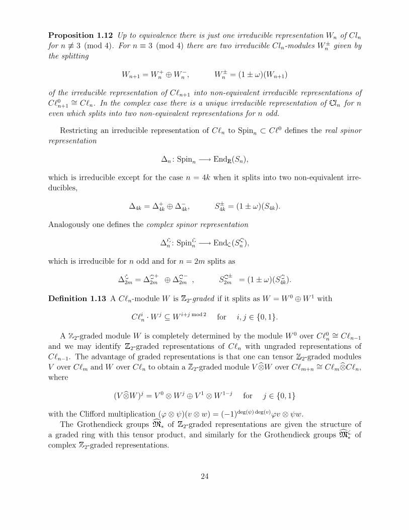
Proposition 1.12 Up to equivalence there is just one irreducible representation Wn of Clnfor n ≡ 3 (mod 4). For n ≡ 3 (mod 4) there are two irreducible Cln-modules W±
n given by
the splitting
Wn+1 = W+n ⊕W−
n , W±n = (1 ± ω)(Wn+1)
of the irreducible representation of Cn+1 into non-equivalent irreducible representations of
C0n+1∼= Cn. In the complex case there is a unique irreducible representation of ln for n
even which splits into two non-equivalent representations for n odd.
Restricting an irreducible representation of Cn to Spinn ⊂ C0 defines the real spinor
representation
∆n : Spinn −→ End(Sn),
which is irreducible except for the case n = 4k when it splits into two non-equivalent irre-
ducibles,
∆4k = ∆+4k ⊕ ∆−4k, S±4k = (1 ± ω)(S4k).
Analogously one defines the complex spinor representation
∆n : Spinn −→ End (Sn ),
which is irreducible for n odd and for n = 2m splits as
∆2m = ∆
2m
+ ⊕ ∆2m
−, S2m
±= (1 ± ω)(S4k).
Definition 1.13 A Cn-module W is 2-graded if it splits as W = W 0 ⊕W 1 with
Cin ·W j ⊆ W i+j mod 2 for i, j ∈ 0, 1.
A 2-graded module W is completely determined by the module W 0 over C0n∼= Cn−1
and we may identify 2-graded representations of Cn with ungraded representations of
Cn−1. The advantage of graded representations is that one can tensor 2-graded modules
V over Cm and W over Cn to obtain a 2-graded module V ⊗W over Cm+n∼= Cm⊗Cn,
where
(V ⊗W )j = V 0 ⊗W j ⊕ V 1 ⊗W 1−j for j ∈ 0, 1
with the Clifford multiplication (ϕ⊗ ψ)(v ⊗ w) = (−1)deg(ψ) deg(v)ϕv ⊗ ψw.
The Grothendieck groups ∗ of 2-graded representations are given the structure of
a graded ring with this tensor product, and similarly for the Grothendieck groups ∗ of
complex 2-graded representations.
24

Clifford and spinor bundles
The Clifford algebra and module constructions above can be extended from vector spaces
with a quadratic form q to vector bundles E over a Riemannian manifold (M, g), where the
fibres of E have an inner product induced from g.
Recall that E is orientable if the first Stiefel–Whitney class w1(E) vanishes. If
wE : H0(On;2) → H1(M ;2)
is the connecting map defined by the fibration
On → PO(E) → M
of orthonormal frames in E, we can write w1(E) = wE(g1) where g1 generates H0(On;2).
If w2(E) = 0 then the orientations correspond to elements of
H0(M,2) ∼= ker(H0(PO(E);2) → H0(On;2)).
Given an orientation we can consider the bundle PSO(E) of positively oriented orthonormal
frames. Orientability is used to define Clifford algebras in this context.
Definition 1.14 The Clifford bundle of an oriented vector bundle E is given by
C(E) = PSO(E) ×SOn Cn,
the bundle associated to the canonical action of SOn on C(n). Alternatively, it is a quotient
of the tensor product bundle
C(E) =∞⊕j=0
E⊗j/
(v ⊗ v + q(v)) .
There is a unique involution α of C(E) extending v → −v on E and an eigenbundle
decomposition
C(E) = C0(E) ⊕ C1(E).
Furthermore, one has a vector bundle isometry
Λ∗E∼=−→ C(E)
which identifies ΛevenE and ΛoddE with C0(E) and C1(E) respectively.
Definition 1.15 A spin structure on E is a double cover
PSpin(E) → PSO(E)
whose restriction to the fibre SOn of π : PSO(E) → X is non-trivial.
25

The obstruction to the existence of a spin structure is the second Stiefel–Whitney class
w2(E). If
wE : H1(SOn;2) → H2(M ;2)
is now the connecting map defined by the fibration
SOn → PSO(E) → M
then w2(E) = wE(g2) where g2 generates H1(SOn;2). If w2(E) vanishes then spin structures
correspond to elements of
H1(M,2) ∼= ker(H1(PSO(E);2) → H1(SOn;2)).
Definition 1.16 A spin manifold is an oriented Riemannian manifold whose tangent bundle
admits a spin structure. The spin cobordism group ΩSpinn is the abelian group generated by
compact connected n-dimensional spin manifolds modulo the relations [N1] + [N2] = 0 if
there is a spin and orientation preserving diffeomorphism N1 N2 → δM for some compact
connected spin (n+ 1)-manifold M .
Spin structures are necessary to extend Clifford modules to vector bundles.
Definition 1.17 A real or complex spinor bundle of an oriented vector bundle E with spin
structure PSpin(E) → PSO(E) is an induced bundle
SW (E) = PSpin(E) ×SpinnW,
where W is a Cn- or n -module. If W is 2-graded, then so is the spinor bundle.
The action of the Clifford algebra on W induces an action of bundles
C(E) ⊕ SW (E) −→ SW (E).
Two spinor bundles are equivalent if they are equivalent as bundles of C(E)-modules and
irreducible if the C(Ex)-module at each fibre is irreducible. If E is a bundle over a connected
n-manifold, it follows from Proposition 1.12 that there is a unique irreducible spinor bundle
Sn(E), or Sn (E), unless n + 1 is divisible by 4, or by 2 in the complex case.
The irreducible spinor bundles S4k(E) and S2m decompose as a direct sum of irreducible
C0(E)-modules S±(E) or S± (E), where
S±(E) = (1 ± ω)(S4k(E)) = PSpin(E) ×∆±4kS±4k,
S± (E) = (1 ± ω )(S2m(E)) = PSpin(E) ×∆
2m± S2m
±.
These correspond to the two irreducible 2-graded spinor bundles in these dimensions.
26

Chapter 2
Some tools from algebraic topology
In this chapter we review some essentials from the theory of characteristic classes, cobordism
theory, and elliptic cohomology. In the first section we recall the definition of Hirzebruch
genera of elliptic type for manifolds with geometric structure. This is a broad (and fasci-
nating) field and we are by no means exhaustive in our presentation. We also recall the
definition of Devoto’s equivariant elliptic cohomology and its modularity properties.
We also discuss some approaches to ‘relative’ versions of the classical theory of characteris-
tic classes and multiplicative sequences, relating them to constructions in relative cobordism
and K-theory. Some aspects of the Pontrjagin–Thom construction for framed bordism, col-
lapse maps on disks and relative characteristic classes are reviewed for the benefit of the
forthcoming exposition.
2.1 Elliptic genera and cohomology theories
We begin by recalling the definitions of Hirzebruch genera and elliptic genera for various
cobordism rings of smooth manifolds with boundary and equipped with a fixed geometric
structure. We will concentrate on SO-structures, but the presentation can be easily adapted
to other geometric structures such as Spin, Spinc, U, SU or String. We will also concentrate
on the case of the classical level two elliptic genus, which is related to the signature operator.
We next recall the G-equivariant elliptic genus introduced by Devoto [Dev98], for G a
finite group of odd order, and the algebraic descriptions of the coefficient and cohomology
rings for the associated generalised cohomology theories, which will be relevant later for one
of our generalisations of the Atiyah–Patodi–Singer construction.
To avoid too much digression in this section we have omitted many interesting aspects of
the theory presented. These include a discussion of important genera of more general elliptic
type, such as the Witten genus, a Spinc elliptic Todd genus, and generalised Eisenstein
genera. Tamanoi’s description [Tam99] of elliptic genera in terms of vertex operator algebras
is also interesting for its relation to the Segal category and Virasoro bundles. In later work
we will also consider elliptic genera modulo n, for n an odd integer, since as was already seen
by [Dev96a] they give rise to invariants for /n-manifolds in the sense of Sullivan, closely
27

related to the invariants we consider. It will then be necessary to consider also the divided
congruence rings of [Kat75] and modular forms modulo prime ideals of [Lau99].
2.1.1 Classical elliptic genera and level 2 elliptic cohomology
Definition 2.1 A genus, in the sense of [Hir66], is a ring homomorphism from the oriented
bordism ring to a commutative -algebra with unit,
φ : ΩSO∗ → R.
In [Tho54], Thom showed that modulo torsion the bordism ring is generated by the
cobordism classes of the even-dimensional complex projective spaces. More explicitly, the
map [ P2k ] → x4k defines an isomorphism of graded rings
ΩSO∗ ⊗ [1
2] ∼= [1
2][x4, x8, x12, . . . ].
A genus φ is uniquely determined by its values on these generators, and hence by the following
formal power series, termed the logarithm of the genus:
g(x) = x+∑k≥1
φ(P2k )x2k+1
2k + 1.
Alternatively, a genus may be specified by
• a total Hirzebruch class P ∈ ∏i≥0Hi(BSO;R), or by
• a characteristic series
P (u) = 1 +∑k≥1
rku2k
in∏
i≥0Hi( P∞ ;R) = R[[u]], u ∈ H2( P∞).
These descriptions determine the genus by the formulas
φ(X) = P(TX)[X]
g−1(u) = u/P (u);
see [Gal96, HBJ92] for further details.
Definition 2.2 [Och87] An elliptic genus is a genus φ : ΩSO∗ → R whose logarithm satisfies
g(x) =
∫ x
0
(1 − 2δt2 + εt4)−12dt
for some δ, ε ∈ R.
28
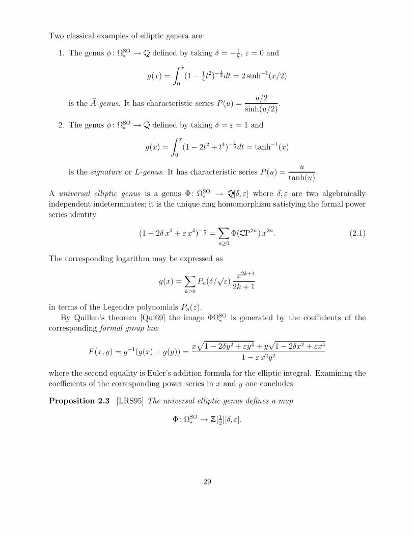
Two classical examples of elliptic genera are:
1. The genus φ : ΩSO∗ → defined by taking δ = −1
8, ε = 0 and
g(x) =
∫ x
0
(1 − 14t2)−
12dt = 2 sinh−1(x/2)
is the A-genus. It has characteristic series P (u) =u/2
sinh(u/2).
2. The genus φ : ΩSO∗ → defined by taking δ = ε = 1 and
g(x) =
∫ x
0
(1 − 2t2 + t4)−12dt = tanh−1(x)
is the signature or L-genus. It has characteristic series P (u) =u
tanh(u).
A universal elliptic genus is a genus Φ: ΩSO∗ → [δ, ε] where δ, ε are two algebraically
independent indeterminates; it is the unique ring homomorphism satisfying the formal power
series identity
(1 − 2δ x2 + ε x4)−12 =
∑n≥0
Φ( P2n) x2n. (2.1)
The corresponding logarithm may be expressed as
g(x) =∑k≥0
Pn(δ/√ε)
x2k+1
2k + 1
in terms of the Legendre polynomials Pn(z).
By Quillen’s theorem [Qui69] the image ΦΩSO∗ is generated by the coefficients of the
corresponding formal group law
F (x, y) = g−1(g(x) + g(y)) =x√
1 − 2δy2 + εy4 + y√
1 − 2δx2 + εx4
1 − ε x2y2
where the second equality is Euler’s addition formula for the elliptic integral. Examining the
coefficients of the corresponding power series in x and y one concludes
Proposition 2.3 [LRS95] The universal elliptic genus defines a map
Φ: ΩSO∗ → [1
2][δ, ε].
29
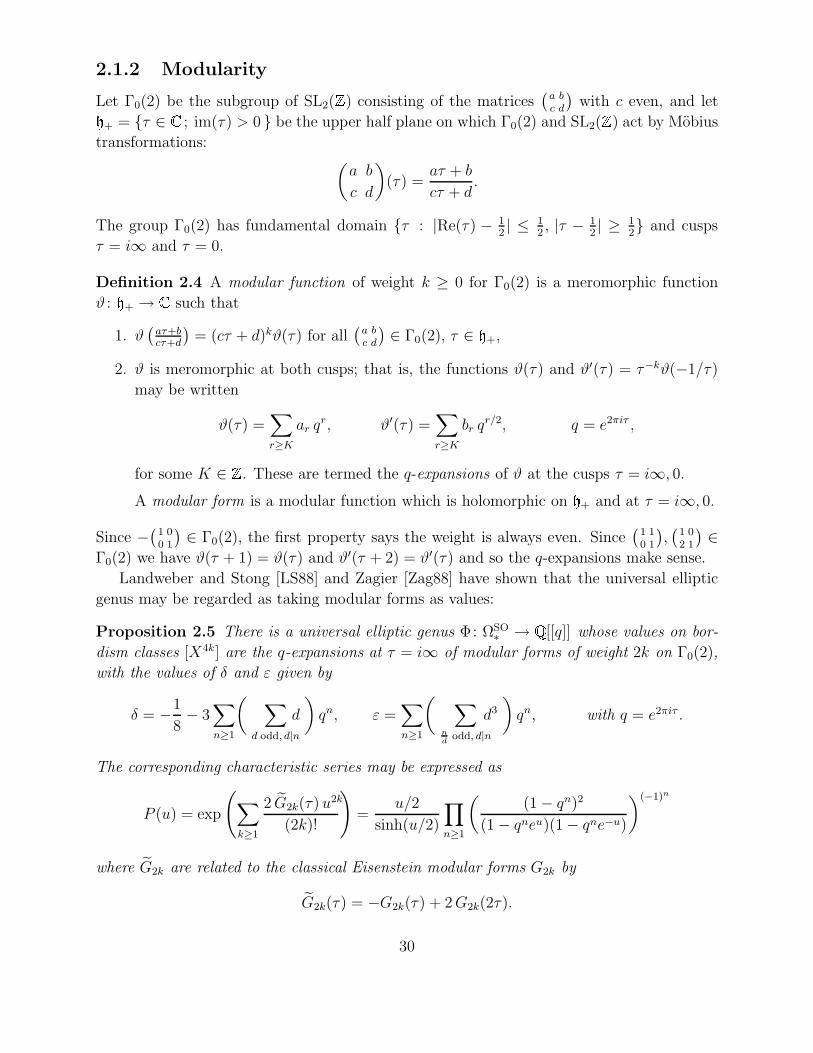
2.1.2 Modularity
Let Γ0(2) be the subgroup of SL2() consisting of the matrices(acbd
)with c even, and let
+ = τ ∈ ; im(τ) > 0 be the upper half plane on which Γ0(2) and SL2() act by Mobius
transformations: (a
c
b
d
)(τ) =
aτ + b
cτ + d.
The group Γ0(2) has fundamental domain τ : |Re(τ) − 12| ≤ 1
2, |τ − 1
2| ≥ 1
2 and cusps
τ = i∞ and τ = 0.
Definition 2.4 A modular function of weight k ≥ 0 for Γ0(2) is a meromorphic function
ϑ : + → such that
1. ϑ(aτ+bcτ+d
)= (cτ + d)kϑ(τ) for all
(acbd
) ∈ Γ0(2), τ ∈ +,
2. ϑ is meromorphic at both cusps; that is, the functions ϑ(τ) and ϑ′(τ) = τ−kϑ(−1/τ)
may be written
ϑ(τ) =∑r≥K
ar qr, ϑ′(τ) =
∑r≥K
br qr/2, q = e2πiτ ,
for some K ∈ . These are termed the q-expansions of ϑ at the cusps τ = i∞, 0.
A modular form is a modular function which is holomorphic on + and at τ = i∞, 0.
Since −(10
01
) ∈ Γ0(2), the first property says the weight is always even. Since(
10
11
),(
12
01
) ∈Γ0(2) we have ϑ(τ + 1) = ϑ(τ) and ϑ′(τ + 2) = ϑ′(τ) and so the q-expansions make sense.
Landweber and Stong [LS88] and Zagier [Zag88] have shown that the universal elliptic
genus may be regarded as taking modular forms as values:
Proposition 2.5 There is a universal elliptic genus Φ: ΩSO∗ → [[q]] whose values on bor-
dism classes [X4k] are the q-expansions at τ = i∞ of modular forms of weight 2k on Γ0(2),
with the values of δ and ε given by
δ = −1
8− 3
∑n≥1
( ∑d odd, d|n
d
)qn, ε =
∑n≥1
( ∑nd
odd, d|nd3
)qn, with q = e2πiτ .
The corresponding characteristic series may be expressed as
P (u) = exp
(∑k≥1
2 G2k(τ) u2k
(2k)!
)=
u/2
sinh(u/2)
∏n≥1
((1 − qn)2
(1 − qneu)(1 − qne−u)
)(−1)n
where G2k are related to the classical Eisenstein modular forms G2k by
G2k(τ) = −G2k(τ) + 2G2k(2τ).
30

Later in this thesis it will sometimes be convenient to identify modular forms for Γ0(2) with
their q-expansions at the other cusp. The corresponding characteristic series P ′ is then given
by P ′(τ, u) = P (−12τ, uτ), or explicity:
P ′(u) = exp
(∑k≥1
4G∗2k(τ) u2k
(2k)!
)=
u/2
tanh(u/2)
∏n≥1
(1 + qneu)(1 + qne−u)(1 − qneu)(1 − qne−u)
· a(q) .
Here G∗2k(τ) = G2k(τ) − 22k−1G2k(2τ) and the normalising factor a(q), necessary so that
P ′(0) = 1, may be written in terms of the Dedekind η-function as
a(q) = η(q)4η(q2)−2, where η(q) = q1/24∏n≥1
(1 − qn).
The q-expansions of the parameters δ, ε at this cusp are
δ =1
4+ 6
∑n≥1
( ∑d odd, d|n
d
)qn, ε =
a(q)4
16=
1
16+∑n≥1
(∑d|n
(−1)dd3
)qn.
With motivation from physics, and assuming that the manifold X has a spin structure,
Witten [Wit88] has shown that P ′ may be considered as giving an expression for the S1-
equivariant index of the Dirac–Ramond operator on an infinite-dimensional manifold of free
smooth loops on X. This ‘explains’ why modular forms arising as genera of spin manifolds
always have q-expansions with integer coefficients.
The elements δ, ε are algebraically independent modular forms of weight 2 and 4 respec-
tively and in fact generate the ring of modular forms for Γ0(2). In [LRS95] it is shown
that the image [12][δ, ε] of Φ is precisely the subring of modular forms whose q-expansion
coefficients at τ = i∞ lie in [12]. It is also shown that on inverting the discriminant
∆ = ε(δ2 − ε)2
of the Jacobi quartic y2 = 1 − 2δx2 + εx4, the ring [12][δ, ε][∆−1] coincides with the mod-
ular functions with q-expansion coefficients in [12] which are holomorphic on + but not
necessarily at the cusps.
2.1.3 Elliptic cohomology theories and the Miller character
For every element ω of positive degree in [12][δ, ε] there is a functor defined on CW-complexes
by
(Eω)∗(X) = MSO∗(X) ⊗ΩSO∗ [12][δ, ε, ω−1].
As proved in [LRS95] and [Fra92], this functor satisfies the axioms of a generalised homology
theory, since after inverting ω the Landweber Exact Functor Theorem applies. The dual
31

cohomology theory, defined using the Spanier–Whitehead duality operator, may be expressed
when X is a finite CW-complex as
(Eω)∗(X) = MSO∗(X) ⊗Ω∗SO[1
2][δ, ε, ω−1].
For the usual choice of ω = ∆ = ε(δ2 − ε)2 we write simply E∗(X).
The Miller character, defined in [Mil89], is a natural transformation of multiplicative
cohomology theories of the form
λ : E∗ → KO∗[12][[q]].
The importance of the Miller character is that the composite
E∗ λ−→ KO∗[12][[q]]
c−→ K∗[12][[q]]
ch−→ H∗ [[q]] (2.2)
defined via the complexification c from KO- to K-theory and the Chern character from
K-theory to ordinary cohomology, is closely related to the elliptic genus.
In the case X = pt, the Miller character on the coefficient rings is just the graded ring
homomorphism
[12][δ, ε][∆−1]
λ∗−→ [12][v2][[q]]
ϑ(τ) → v2k ϑ(q)
which sends a modular function ϑ(τ) of weight 4k to its q-expansion at the cusp τ = i∞; in
particular the images of δ and ε are the formal power series given in described in Proposi-
tion 2.5. Here v2 = y is the usual generator for KO[12]-theory, in degree 4.
For X = P∞ we have the complex orientation class xE ∈ E2( P1), with
E∗( P∞) ∼= E∗[[xE ]],
and the Miller character is determined by its value tKE (xE) on xE ,
tKE (xε) = xK∏n≥1
(1 − qnv2(xK)2
(1 − qn)2
)(−1)n
.
On applying the Chern character to the complexification we obtain
ch(tKE (xε)
)=(e
x2 − e
−x2
)∏n≥1
(1 − qnv2 (ex + e−x − 2)
(1 − qn)2
)(−1)n
which is just the class x/P (x) where P is the characteristic series for the elliptic genus given
in Proposition 2.5.
In fact this series corresponds to the q-expansion of the Jacobi elliptic sine sE
ch(tKE (xε)
)= sE (τ, x) = (℘ (τ, x) − eε (τ))−
12
32

which is known to be a Jacobi meromorphic form of weight −1 and index 0. From the
general theory of Hirzebruch genera [Hir66], computation of the universal elliptic genus of
any projective space P2k involves only taking derivatives and evaluation, and in general we
may identify the modular forms obtained with Jacobi forms of index 0:
E∗ ( P∞) ∼= E∗ [[xε]] → J mer∗,0
(Γ0(2);[1
2]).
In terms of theta functions we may also write
sE(τ, x)−1 = ε14
ϑ( 12,0)(τ, x
2πi
)ϑ( 1
2, 12)(τ, x
2πi
) ;see [Dev96b, EZ85] for more details.
2.1.4 Equivariant elliptic cohomology
In [Dev98], Devoto showed that for any finite group G of odd order one may define a sta-
ble G-equivariant cohomology theory on finite G-CW-complexes, termed equivariant elliptic
cohomology, by
E∗G(X) = MSO∗G(X) ⊗MSO∗G
E∗G (2.3)
where MSO∗G is -graded oriented equivariant cobordism theory [CW89]. The graded ring
E∗G = E∗G(pt) is related to the moduli space of G-coverings of Jacobi quartics, and comes
equipped with a universal twisted elliptic genus
ΦG : MSO∗G −→ E∗G. (2.4)
This is the G-equivariant version of the definition of ordinary elliptic cohomology by
E∗G(X) = MSO∗(X) ⊗MSO∗ E∗
where the coefficient ring E∗ ∼= [12][δ, ε][∆−1] is the graded ring of modular functions which
are holomorphic away from the cusps and have q-expansion coefficients in [12], as above. If
X has a free G-action, then E∗GX will be isomorphic to E∗(X/G) ⊗ [
1|G|
].
For the equivariant case, Devoto makes an appropriate generalisation of the notion of
“modular form”. Let TG = (x, y) ∈ G2 ; [x, y] = 1 be the set of pairs of commuting
elements of G. Then the usual action of Γ0(2) on + as usual and the conjugation action
of G on TG are are combined to give actions ρk of Γ0(2) × G on the ring of functions
ϑ : TG× + → ,
ρk(A, g)ϑ : ((x, y), τ) −→ (cτ + d)−k ϑ(
( gxdy−cg−1, gx−byag−1),aτ + b
cτ + d
)(2.5)
for k ∈ , A =(acbd
) ∈ Γ0(2), g ∈ G and ((x, y), τ) ∈ TG× +.
We write ζj for the primitive jth root of unity e2πi/j ∈ .
33

Definition 2.6 The graded ring E∗G =⊕ E−2k
G is the ring of functions ϑ : TG×+ → satisfying the following conditions, for some k ∈ :
1. ρk(A, g)ϑ = ϑ for all (A, g) ∈ Γ0(2) ×G,
2. for each (x, y) ∈ TG the function ϑ((x, y), τ) is holomorphic, and is meromorphic at
the cusps; that is, the functions ϑ((x, y), τ) and ϑ′((x, y), τ) = τ−kϑ((x, y),− 1τ) have
q-expansions
ϑ((x, y), τ) =∑r≥K
ar qr/|x|, ϑ′((x, y), τ) =
∑r≥K
br qr/|x|, q = e2πiτ , (2.6)
for some K ∈ ,
3. the coefficients ar(x, y), br(x, y) lie in [
12, 1|G| , ζ|xy|
]and satisfy
σn(ar(x, y)) = ar(x, yn), σn(br(x, y)) = br(x, y
n) (2.7)
for σn a ring automorphism of [
12, 1|G| , ζm
]given by σn(ζm) = ζm
n for any n coprime
to m, where m is the order of the centraliser CG(x).
The third condition says that for each x ∈ G the coefficient functions ar(x,−), br(x,−) :
CG(x) → are elements of R(CG(x)) ⊗ [12], where R(CG(x)) is the character ring of the
centraliser.
In Devoto’s papers [Dev96a, Dev96b, Dev98], the identification of coefficient rings E∗Gas modular forms ones is extensively developed. We will give a partial account only without
introducing the formalism of schemes, but instead by applying the following result by Eichler
and Zagier [EZ85].
Theorem 2.7 Let φ be a Jacobi form on Γ of weight k and index m and λ, µ rational
numbers. Then, the function
f (τ) = e2πiλ2τφ (τ, λτ + µ)
is a modular form of weight k and on some subgroup Γ′ of finite index depending only on Γ
and on λ, µ. In particular, for λ = µ = 0, f (τ) is a modular form for Γ.
According to the description in the proof of this theorem, the group Γ′ can be written
explicitly as
Γ′ =(
a b
c d
)∈ Γ : (a− 1)λ+ cµ, bλ+ (d− 1)µ,m(cµ2 + (d− a)λµ− bλ2) ∈
and hence this group contains Γ∩Γ
(N2
(N,m)
)if N (λ, µ) ∈ 2. We are interested in particular
in generalised Jacobi forms and functions coming from the Weierstrass ℘ function, for which
one obtains the Teilwerte [Ogg69]
f (ω1, ω2, N, a1, a2) = ℘(a1ω1
N+ a2
ω2
N,ω1, ω2
),
which is a modular form of weight 2 and level N , for a given lattice (ω1, ω2) and integers N ,
(a1, a2) = (0, 0).
34

2.2 Relative cobordism theories and classes
In this section we review some fundamental constructions from cobordism theory and the
related differential topology. We recall the notions of cobordism categories and (B, f)-
constructions, and we describe their ‘relative’ versions, especially for the case of relative
cobordism of oriented (or almost complex manifolds) with framed boundary.
We discuss the Pontrjagin–Thom construction and Kervaire’s account of relative Chern
classes. The corresponding relative multiplicative sequences turn out to be just reduced mul-
tiplicative sequences, leading to relative characteristic numbers following Stong’s definition.
2.2.1 Relative characteristic classes
We recall Kervaire’s account of relative characteristic classes in ordinary cohomology [Ker57]
and summarise their properties.
Definition 2.8 Let
B =(EU(n), p, BU(n),U(n)
)be the classifying bundle for U(n). Suppose that a cross section θr over a closed subset A of
BU(n) is given in the associated bundle
Br =(EU(n), p, BU(n),U(n),Wn, n−r
)with fibre Wn, n−r, the complex Stiefel manifold of n − r complex vectors in n . Then, for
j ≥ r, the relative Chern classes
cRj (Br) ∈ H2(j+1)(BU(n), A;
)corresponding to the cross section θr will be defined by the properties:
1. For the natural homomorphism a∗ : H∗(BU(n), A;
) → H∗(BU(n);
)induced by the
inclusion a :(BU(n), 0
) → (BU(n), A
)one has
a∗(cRj+1 (Br)
)= cj+1 (Br)
the usual (i.e., absolute) Chern classes.
2. For the homomorphism ρ∗j,n : H∗(BU(n), A;
) → H∗(BU(j), θ
jA;)
induced by the
Borel map ρ (U(j),U(n)) one has
ρ∗j,n(cRj+1 (Br)
)= 0.
35
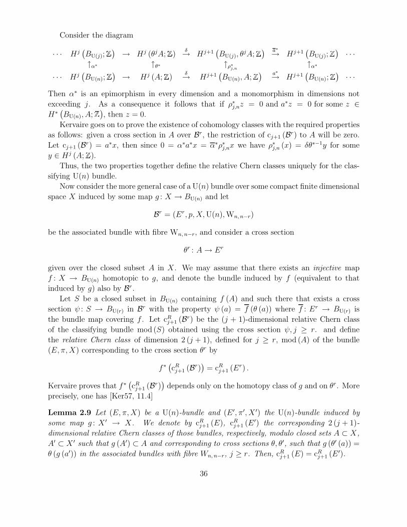
Consider the diagram
· · · Hj(BU(j);
) → Hj (θjA;)δ→ Hj+1
(BU(j), θ
jA;) a∗→ Hj+1
(BU(j);
) · · ·↑α∗ ↑θ∗ ↑ρ∗j,n
↑α∗
· · · Hj(BU(n);
) → Hj (A;)δ→ Hj+1
(BU(n), A;
) a∗→ Hj+1(BU(n);
) · · ·Then α∗ is an epimorphism in every dimension and a monomorphism in dimensions not
exceeding j. As a consequence it follows that if ρ∗j,nz = 0 and a∗z = 0 for some z ∈H∗(BU(n), A;
), then z = 0.
Kervaire goes on to prove the existence of cohomology classes with the required properties
as follows: given a cross section in A over Br, the restriction of cj+1 (Br) to A will be zero.
Let cj+1 (Br) = a∗x, then since 0 = α∗a∗x = α∗ρ∗j,nx we have ρ∗j,n (x) = δθ∗−1y for some
y ∈ Hj (A;).
Thus, the two properties together define the relative Chern classes uniquely for the clas-
sifying U(n) bundle.
Now consider the more general case of a U(n) bundle over some compact finite dimensional
space X induced by some map g : X → BU(n) and let
Br = (Er, p,X,U(n),Wn,n−r)
be the associated bundle with fibre Wn, n−r, and consider a cross section
θr : A → Er
given over the closed subset A in X. We may assume that there exists an injective map
f : X → BU(n) homotopic to g, and denote the bundle induced by f (equivalent to that
induced by g) also by Br.
Let S be a closed subset in BU(n) containing f (A) and such there that exists a cross
section ψ : S → BU(r) in Br with the property ψ (a) = f (θ (a)) where f : Er → BU(r) is
the bundle map covering f . Let cRj+1 (Br) be the (j + 1)-dimensional relative Chern class
of the classifying bundle mod (S) obtained using the cross section ψ, j ≥ r. and define
the relative Chern class of dimension 2 (j + 1), defined for j ≥ r, mod (A) of the bundle
(E, π,X) corresponding to the cross section θr by
f ∗(cRj+1 (Br)
)= cRj+1 (Er) .
Kervaire proves that f ∗(cRj+1 (Br)
)depends only on the homotopy class of g and on θr. More
precisely, one has [Ker57, 11.4]
Lemma 2.9 Let (E, π,X) be a U(n)-bundle and (E ′, π′, X ′) the U(n)-bundle induced by
some map g : X ′ → X. We denote by cRj+1 (E), cRj+1 (E ′) the corresponding 2 (j + 1)-
dimensional relative Chern classes of those bundles, respectively, modulo closed sets A ⊂ X,
A′ ⊂ X ′ such that g (A′) ⊂ A and corresponding to cross sections θ, θ′, such that g (θ′ (a)) =
θ (g (a′)) in the associated bundles with fibre Wn, n−r, j ≥ r. Then, cRj+1 (E) = cRj+1 (E ′).
36

Let B1 and B2 be two principal bundles with bundle groups U(n1) and U(n2) respectively,
over the same base space X and let θr1 , θr2 be cross sections over closed subsets A1, A2 of X
in the associated bundles Br11 and Br2
2 with fibres Wn1, n1−r1,Wn2, n2−r2 , respectively. Then
θr1 , θr2 determine a cross section θr, r = r1+r2, over A = A1 ∩A2 in the bundle Br1 with fibre
Wn, n−r, n = n1 +n2 associated to the Whitney sum B = B1 ⊕B2. Let cRj+1 (B1) , cRj+1 (B2) be
the relative Chern class of B1,B2, defined for j ≥ r1, r2, respectively, and let cRj+1 (B) be the
relative Chern class of B, defined for j ≥ r. For the relative Chern classes, Whitney duality
takes the form
cRj+1 (Br) = cRj+1 (B1) + · · · + cRj (B1) c1 (B2) + · · · + cRj+1 (B2)
where some absolute Chern classes occur. However, since each product contains at least one
relative class, it is itself a relative class.
2.2.2 Relative multiplicative sequences
Let K be a multiplicative sequence in the sense of [Hir66] in Chern classes of bundles. Denote
by∼K the corresponding reduced classes, defined as follows. For a bundle ξ,
K• (ξ) = 1+∼K• (ξ) .
Because of the multiplicativity of K, one has
K• (ξ1 ⊕ ξ2) = K• (ξ1) · K• (ξ2)
1+∼K• (ξ1 ⊕ ξ2) =
(1+
∼K• (ξ1)
)·(1+
∼K• (ξ2)
)and hence
∼K• (ξ1 ⊕ ξ2) =
∼K• (ξ1)+
∼K• (ξ2) +
∼K• (ξ1)
∼K• (ξ2) .
Now, if one considers relative characteristic classes in the sense of Kervaire as described
before, in the particular case of r = 0, then θ0 will determine further relative characteristic
classes given by
∼K• (ξ1) = KR
• (ξ1) .
Hence
KR• (ξ1 ⊕ ξ2) = KR
• (ξ1) + KR• (ξ2) + KR
• (ξ1) KR• (ξ2) .
37
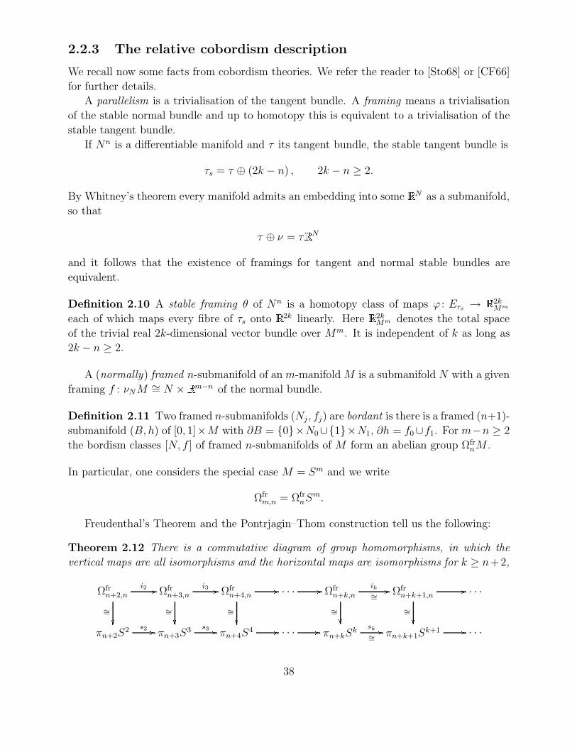
2.2.3 The relative cobordism description
We recall now some facts from cobordism theories. We refer the reader to [Sto68] or [CF66]
for further details.
A parallelism is a trivialisation of the tangent bundle. A framing means a trivialisation
of the stable normal bundle and up to homotopy this is equivalent to a trivialisation of the
stable tangent bundle.
If Nn is a differentiable manifold and τ its tangent bundle, the stable tangent bundle is
τs = τ ⊕ (2k − n) , 2k − n ≥ 2.
By Whitney’s theorem every manifold admits an embedding into some N as a submanifold,
so that
τ ⊕ ν = τN
and it follows that the existence of framings for tangent and normal stable bundles are
equivalent.
Definition 2.10 A stable framing θ of Nn is a homotopy class of maps ϕ : Eτs → 2kMm
each of which maps every fibre of τs onto 2k linearly. Here 2kMm denotes the total space
of the trivial real 2k-dimensional vector bundle over Mm. It is independent of k as long as
2k − n ≥ 2.
A (normally) framed n-submanifold of an m-manifold M is a submanifold N with a given
framing f : νNM ∼= N × m−n of the normal bundle.
Definition 2.11 Two framed n-submanifolds (Nj , fj) are bordant is there is a framed (n+1)-
submanifold (B, h) of [0, 1]×M with ∂B = 0×N0 ∪1×N1, ∂h = f0 ∪f1. For m−n ≥ 2
the bordism classes [N, f ] of framed n-submanifolds of M form an abelian group ΩfrnM .
In particular, one considers the special case M = Sm and we write
Ωfrm,n = Ωfr
nSm.
Freudenthal’s Theorem and the Pontrjagin–Thom construction tell us the following:
Theorem 2.12 There is a commutative diagram of group homomorphisms, in which the
vertical maps are all isomorphisms and the horizontal maps are isomorphisms for k ≥ n+2,
Ωfrn+2,n
∼=
i2 Ωfr
n+3,n
∼=
i3 Ωfr
n+4,n
∼=
· · · Ωfrn+k,n
∼=
ik∼= Ωfr
n+k+1,n
∼=
· · ·
πn+2S2
s2πn+3S
3 s3
πn+4S4 · · · πn+kS
k sk
∼= πn+k+1Sk+1 · · ·
38

There are therefore isomorphisms between the framed bordism groups Ωfrn = lim
−→ kΩfrn+k,n and
the stable homotopy groups of spheres,
Ωfrn
∼= πsn = lim
−→k
πn+kSk.
In this theorem the maps sk are given by suspension, and ik[N, f ] = [N, f × ] since for
N ⊂ Sm one can identify the normal bundle in Sm+1 as the normal bundle in Sm plus a copy
of the trivial line bundle. The vertical maps are the Pontrjagin–Thom construction, which
uses transversality arguments in differential topology; in general ΩfrnM
n+k ∼= [Mn+k, Sk],
identifying framed n-submanifolds of Mn+k with the zero-sets of maps f : Mn+k → Sk which
are smooth on a neighbourhood of f−1(0) and have 0 as a regular value.
Definition 2.13 The J-homomorphism is the map
J : πn(O(k)) → Ωfrn+k,n
∼= πn+kSk
defined by twisting the normal framing of Sn in Sn+k by a representation of Sn in the
orthogonal group of the fibre. The stable J-homomorphism J : πn(O) → πsn is given by
taking lim−→k
.
Other bordism theories (G, f) are constructed by requiring further structure on the nor-
mal bundle of a smooth manifold. Let G be a sequence of topological groups Gn with
compatible maps Gn → O(n). For example, Gn = O(n), SO(n), Spin(n), U(n/2) will give
ordinary, oriented, spin and complex bordism theories respectively. The stable bordism group
ΩGn (X) is the group of bordism classes of n-submanifolds of Sn+k with maps to X and stable
G-structures on the normal bundle. The Pontrjagin–Thom construction generalises to give
isomorphisms
ΩGn (X) ∼= MGn(X)
where MG is the Thom spectrum of G, with MGn = D(EGn)/S(EGn) the Thom space of
the principal G-bundle EGn → BGn, and
MGn(X) = lim−→k
πn+k(X+ ∧MGk).
In the case of framed cobordism one takes Gn = 1 for all n, and MG is then the sphere
spectrum.
An important point for us to recall is how every stable framing θ of Nn defines a U-
structure. For given ϕ : Eτs → 2kMm , the natural operator J : 2k → 2k given by
J (x1, x2, . . . , x2k−1, x2k) = (−x2, x1, . . . ,−x2k, x2k−1)
pulls back to an operator
J : Eτs → Eτs
39

representing a U-structure θU on Nn. This leads to a homomorphism
r : Ωfrn → ΩU
n
by
[Nn, θ]fr −→ [Nn, θU
]U.
It is clear that, for n > 0, Ωfrn finite and ΩU
n free abelian implies that r = 0. So, given a closed
stably framed manifold Nn with n > 0, then Nn is as well an U-manifold, and one such that
[Nn]U = 0. Hence, there exists a compact U-manifold Mn+1 with ∂Mn+1 = Nn. So, from
now on we are going to consider such pairs (Mn+1, Nn), or, more precisely, (Mn+1, Nn, π),
where π = ∂θ, from θU. Such a triple is a (U-fr)-manifold.
Consider τs the stable tangent bundle of (Mm, ∂Mm) , which is a bundle of k-dimensional
complex vector spaces and one with a trivialisation on its restriction to the boundary: we
are given an isomorphism
ϕ |∂Mm : E(τs|∂Mm ) → 2k|∂Mm .
Recall the definitions for difference elements in K-theory by Atiyah (see [APS75II]
or [LM89]). The isomorphism ϕ |∂Mm determines a difference class
d (τs, k, ϕ) ∈ K (Mn, ∂Mn)
which is denoted as the stable tangent bundle of the (U-fr)-manifold Mn. Sometimes, how-
ever, we will denote this element as
τ = τ (M, ∂M) ∈ K (Mn, ∂Mn) .
For any (G, f)-theory, there is an exact couple
Ωfr∗ → ΩG
∗
ΩG, fr∗
where ΩG, fr∗ are the relative cobordism groups of manifolds with a G structure whose boundary
is given a framing. So, the construction can be performed for G = SO, Spin, Spinc etc, but
it turns out that the simplest statement comes out by using
Ωfr∗ → ΩU
∗
ΩU, fr∗
because in that case for every n > 0, one obtains a short exact sequence
0 → ΩU∗ → ΩU, fr
∗ → Ωfr∗ → 0
40

and elements in ΩU, fr∗ are called cobordism classes of (U, fr).
If M is a (U-fr)-manifold as described above, then it has Chern classes, which we may
write as
ck (M) = ck (τ) ∈ H2k (Mn, ∂Mn)
as defined in [CF66, p. 93]. Then, we may define the Chern numbers of a compact (U-fr)-
manifold by
cI(M2n
)= ci1 · · · ciχ
[M2n
]=⟨
ci1 (M) · · · ciχ (M) , σ (M)⟩,
where
σ (M) ∈ Hn (Mn, ∂Mn)
denotes the orientation class of Mn, Mn being compact. For convenience we remember the
definition for the Chern classes of a vector bundle.
The relative characteristic numbers so obtained may be seen to be consistent with what
is obtained using Kervaire’s description using the more general Stong’s definitions for quite
general theories as explained in [Sto68, p. 32].
Given fibration sequences
Bh→ B
f→ BO
one may think of
y ∈ H∗(B,B;A˜)
as a relative characteristic class, by means of the following procedure. Let M be a (B, f)-
manifold with(B, f h) a structure on its boundary ∂M . In that case, one has defined a
relative characteristic number
y [M, ∂M ] ∈ H∗(pt;A˜)
since the normal map gives (M, ∂M) → (B,B
).
From the algebraic topology point of view, a very interesting feature of such numbers
is that they are relative cobordism invariants. To prove it, Stong uses the fact one may
suppose by additivity that there is a (B, f)-manifold W with ∂W = M ∪ (−U) joined along
∂M ∼= ∂U , with U a(B, f h)-manifold and so one obtains the sequence
(W, ∂W )d−→ Σ (∂W/)
Σj−→ Σ (∂W/U)Σp←− Σ (M/∂M)
which gives out
p∗ [M, ∂M ] = j∗∂ [W, ∂W ]
41

by the orientation assumption in the decomposition of ∂W and y (M, ∂M) = p∗q∗y (W,U)
where
(M, ∂M)p→ (∂W,U)
q→ (W,U)
and
y [M, ∂M ] = 〈q∗y, j∗∂ [W, ∂W ]〉 = 〈δj∗q∗y, [W, ∂W ]〉 .
However, from the exact sequence of the triple (W, ∂W,U) the composition
H∗ (W,U)q∗→ H∗ (∂W,U)
p∗→ H∗ (M, ∂M)
is zero, and hence
y [M, ∂M ] = 0.
Observe as well that taking B = , this reduces to the closed case.
2.2.4 The case of the disk bundles
Suppose we are given Mn a compact smooth orientable manifold with boundary ∂Mn, with
a class x ∈ K (Mn, ∂Mn) such that the composition K (Mn, ∂Mn) → K (Mn) → KO (Mn)
maps x into the class of the stable tangent bundle in KO (Mn). Then x can be used to give
to τs, the stable tangent bundle of (Mn, ∂Mn), the structure of a complex vector bundle
and one with a trivialisation on its restriction to the boundary. That amounts to give a
(U-fr)-manifold structure (not in a unique way!) such that τ (M, ∂M) = x ∈ K (Mn, ∂Mn).
This will give cHk (x) = cHk (M) with the definitions in [CF66].
All this may be applied to (D2n, S2n−1). In this case, there is a class x ∈ K (D2n, ∂S2n−1)
such that ⟨cHk (x) , σ
(D2n
)⟩= (n− 1)!
This can be seen by considering ξ a complex vector bundle arising from the principal spin
bundle on S2n determined by any of the half spin irreducible representations of Spin (2n), so
that⟨cHk (ξ) , σ (S2n)
⟩= (n− 1)! and then considering its pullback under the collapse map
c : D2n D2n/S2n−1 ∼ S2n topologically and using the naturality of the Chern classes. We
are allowed to consider x = [c∗ (ξ)] as an element in K (D2n, ∂S2n−1) giving the class of τs,
since KO (Mn) = 0 in this case and hence the short exact sequence
K (Mn, ∂Mn) → K (Mn) → KO (Mn)
is in fact
K (Mn, ∂Mn) → K (Mn) → 0
42

so any nontrivial element in it will be suitable to become a stable tangent bundle for the
disk. Anyway, we are allowed to take D2n as a (U-fr)-manifold with τ = x. Hence, cobordism
theory ensures the existence of a compact (U-fr)-manifold D2n with cHk [D2n] = (n − 1)! and
all the other Chern numbers are zero because of vanishing of all non-extreme-dimensional
cohomologies in D2n.
According to [Smi71, p. 241], the results from applying ∂∗ to such cells give us an element
in Ωfr2n−1 = πs
2n−1 which is a generator for the image of
J : π2n−1 (U) → πs2n−1.
The usual generator σ ∈ K (S2n) (see for instance [LM89] or [ABS64]) corresponds to the
spin bundle before described and for it one has
cn (σ) = (n − 1)!ι2n ∈ H2n(S2n;
)where ι2n is the corresponding usual generator for cohomology. Use of the Chern character
tells us then that
ch (τ) = e2n ∈ H2n(D2n, S2n−1;
).
Now, for µ ∈ K (D2n, S2n−1) the element corresponding to σ, one has
cn (σ) = (n − 1)!e2n ∈ H2n(D2n, S2n−1;
)and, since KO (D2n) = 0, we may choose µ as a stable tangent bundle for (D2n, S2n−1),
providing it with the required structure of a (U-fr)-manifold. TheK-theoretical characteristic
numbers as described in Stong are computed by [Smi71, p. 242]. For H ∈ K (S2) the
canonical line bundle, we have σ2 = H − 1.
As a consequence, an (SO-fr)-manifold structure on D4k exists such that the Newton
characteristic numbers are
sk[D4k
]= (−1)k kpk
[D4k
]= (2k)!
Consider now(S4k−1, f
)any framed sphere of dimension 4k − 1. The Pontrjagin and
Stiefel–Whitney classes of S4k−1 vanish, so there is a compact oriented disk manifold D4k
with ∂D4k = S4k−1, and a Riemannian one such that on a neighbourhood of the boundary the
metric on the disk is the product metric from the one induced on the sphere by considering
the given framing as orthonormal. Since S4k−1 is framed, the tangent bundle of D4k is pulled
back from a bundle on the quotient space D4k/S4k−1, which in this very special case happens
to be a smooth manifold itself, an S4k. This allows one to define the Pontrjagin classes of
D4k as relative classes pi ∈ H4i(D4k, S4k−1
)and to see them as elements in the reduced
cohomology group H4i(S4k).
In fact, there is as choice for(D4k, S4k−1, f0
)such that D4k is the unit ball in 2k ,
so an almost complex manifold with boundary M = S4k−1, and in fact the almost complex
43
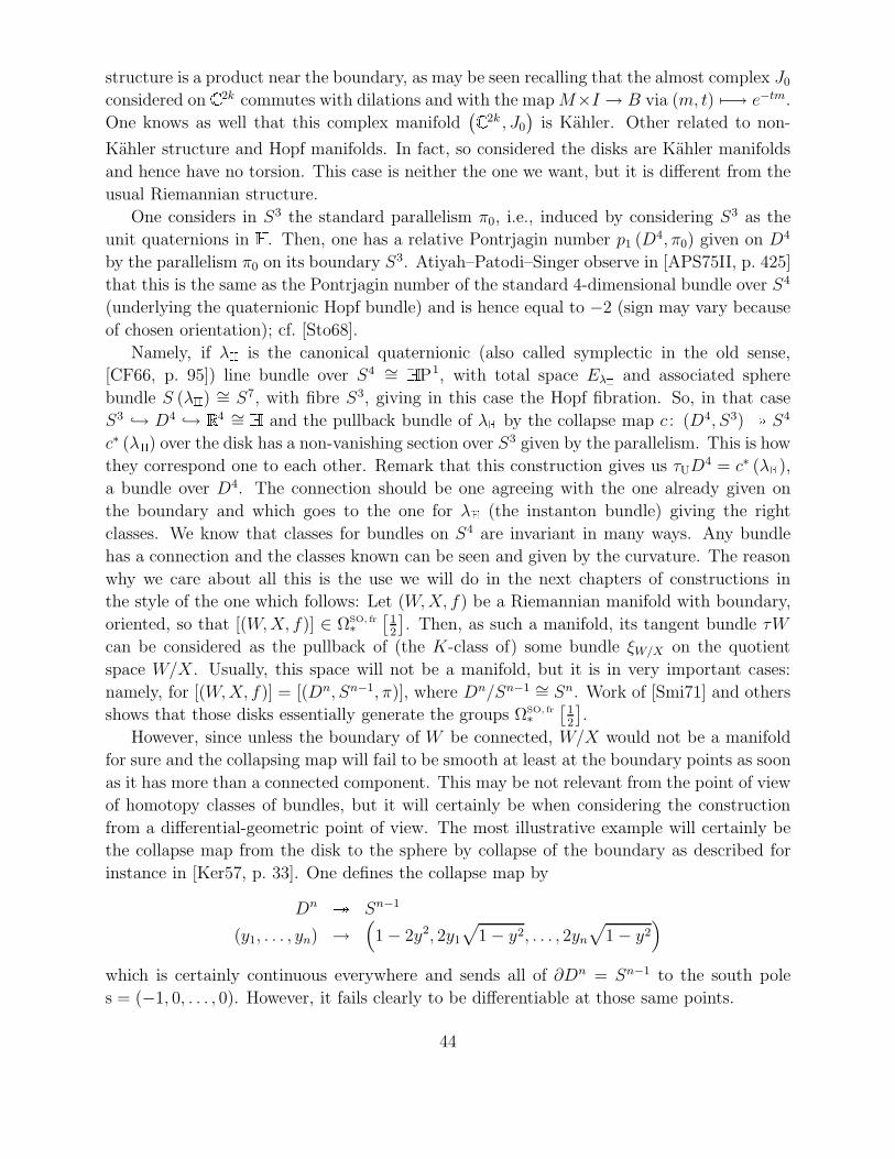
structure is a product near the boundary, as may be seen recalling that the almost complex J0
considered on 2k commutes with dilations and with the mapM×I → B via (m, t) −→ e−tm.
One knows as well that this complex manifold( 2k , J0
)is Kahler. Other related to non-
Kahler structure and Hopf manifolds. In fact, so considered the disks are Kahler manifolds
and hence have no torsion. This case is neither the one we want, but it is different from the
usual Riemannian structure.
One considers in S3 the standard parallelism π0, i.e., induced by considering S3 as the
unit quaternions in . Then, one has a relative Pontrjagin number p1 (D4, π0) given on D4
by the parallelism π0 on its boundary S3. Atiyah–Patodi–Singer observe in [APS75II, p. 425]
that this is the same as the Pontrjagin number of the standard 4-dimensional bundle over S4
(underlying the quaternionic Hopf bundle) and is hence equal to −2 (sign may vary because
of chosen orientation); cf. [Sto68].
Namely, if λ is the canonical quaternionic (also called symplectic in the old sense,
[CF66, p. 95]) line bundle over S4 ∼= P1, with total space Eλ and associated sphere
bundle S (λ ) ∼= S7, with fibre S3, giving in this case the Hopf fibration. So, in that case
S3 → D4 → 4 ∼= and the pullback bundle of λ by the collapse map c : (D4, S3) S4
c∗ (λ ) over the disk has a non-vanishing section over S3 given by the parallelism. This is how
they correspond one to each other. Remark that this construction gives us τUD4 = c∗ (λ ),
a bundle over D4. The connection should be one agreeing with the one already given on
the boundary and which goes to the one for λ (the instanton bundle) giving the right
classes. We know that classes for bundles on S4 are invariant in many ways. Any bundle
has a connection and the classes known can be seen and given by the curvature. The reason
why we care about all this is the use we will do in the next chapters of constructions in
the style of the one which follows: Let (W,X, f) be a Riemannian manifold with boundary,
oriented, so that [(W,X, f)] ∈ ΩSO, fr∗[
12
]. Then, as such a manifold, its tangent bundle τW
can be considered as the pullback of (the K-class of) some bundle ξW/X on the quotient
space W/X. Usually, this space will not be a manifold, but it is in very important cases:
namely, for [(W,X, f)] = [(Dn, Sn−1, π)], where Dn/Sn−1 ∼= Sn. Work of [Smi71] and others
shows that those disks essentially generate the groups ΩSO, fr∗[
12
].
However, since unless the boundary of W be connected, W/X would not be a manifold
for sure and the collapsing map will fail to be smooth at least at the boundary points as soon
as it has more than a connected component. This may be not relevant from the point of view
of homotopy classes of bundles, but it will certainly be when considering the construction
from a differential-geometric point of view. The most illustrative example will certainly be
the collapse map from the disk to the sphere by collapse of the boundary as described for
instance in [Ker57, p. 33]. One defines the collapse map by
Dn Sn−1
(y1, . . . , yn) →(1 − 2y2, 2y1
√1 − y2, . . . , 2yn
√1 − y2
)which is certainly continuous everywhere and sends all of ∂Dn = Sn−1 to the south pole
s = (−1, 0, . . . , 0). However, it fails clearly to be differentiable at those same points.
44
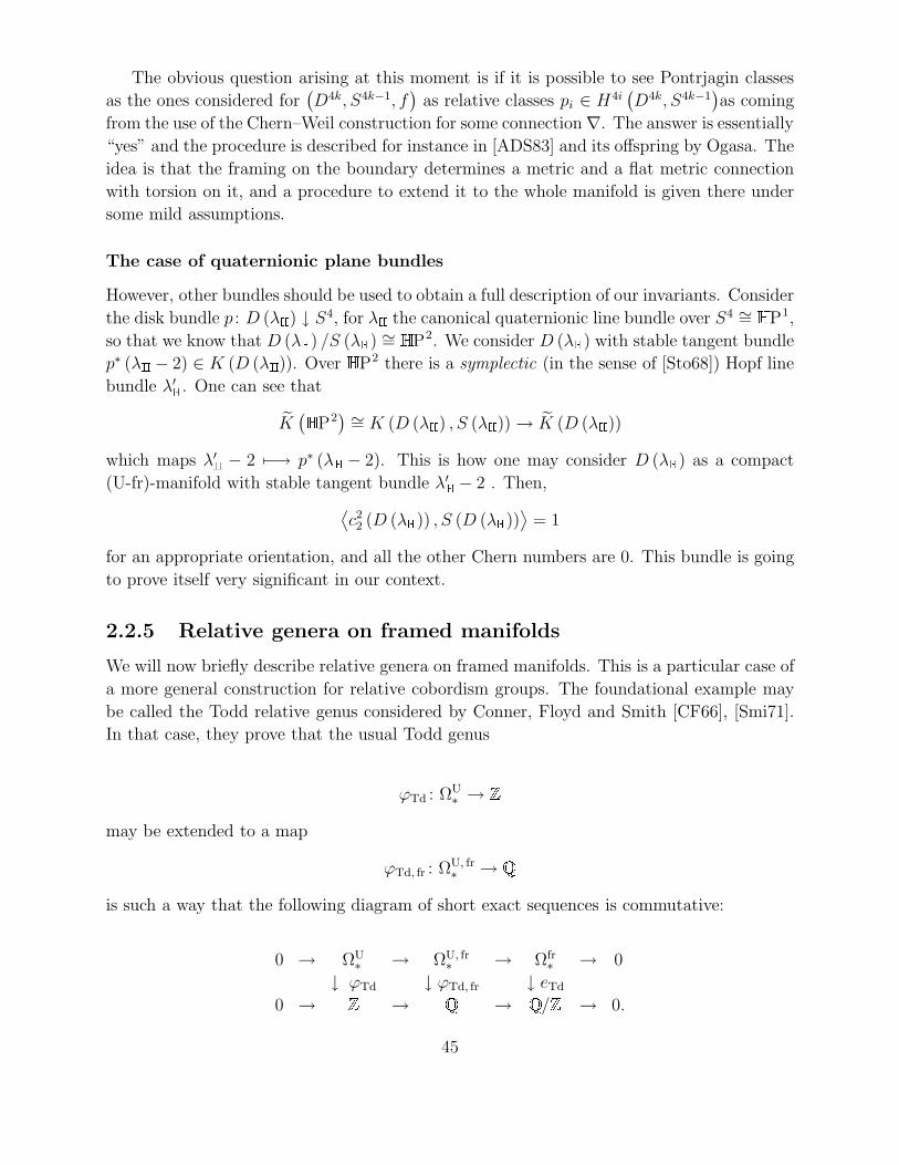
The obvious question arising at this moment is if it is possible to see Pontrjagin classes
as the ones considered for(D4k, S4k−1, f
)as relative classes pi ∈ H4i
(D4k, S4k−1
)as coming
from the use of the Chern–Weil construction for some connection ∇. The answer is essentially
“yes” and the procedure is described for instance in [ADS83] and its offspring by Ogasa. The
idea is that the framing on the boundary determines a metric and a flat metric connection
with torsion on it, and a procedure to extend it to the whole manifold is given there under
some mild assumptions.
The case of quaternionic plane bundles
However, other bundles should be used to obtain a full description of our invariants. Consider
the disk bundle p : D (λ ) ↓ S4, for λ the canonical quaternionic line bundle over S4 ∼= P1,
so that we know that D (λ ) /S (λ ) ∼= P2. We consider D (λ ) with stable tangent bundle
p∗ (λ − 2) ∈ K (D (λ )). Over P2 there is a symplectic (in the sense of [Sto68]) Hopf line
bundle λ′ . One can see that
K( P2
) ∼= K (D (λ ) , S (λ )) → K (D (λ ))
which maps λ′ − 2 −→ p∗ (λ − 2). This is how one may consider D (λ ) as a compact
(U-fr)-manifold with stable tangent bundle λ′ − 2 . Then,⟨c22 (D (λ )) , S (D (λ ))
⟩= 1
for an appropriate orientation, and all the other Chern numbers are 0. This bundle is going
to prove itself very significant in our context.
2.2.5 Relative genera on framed manifolds
We will now briefly describe relative genera on framed manifolds. This is a particular case of
a more general construction for relative cobordism groups. The foundational example may
be called the Todd relative genus considered by Conner, Floyd and Smith [CF66], [Smi71].
In that case, they prove that the usual Todd genus
ϕTd : ΩU∗ →
may be extended to a map
ϕTd, fr : ΩU, fr∗ →
is such a way that the following diagram of short exact sequences is commutative:
0 → ΩU∗ → ΩU, fr
∗ → Ωfr∗ → 0
↓ ϕTd ↓ ϕTd, fr ↓ eTd
0 → → → / → 0.
45

In particular, for the disks(D4k, S4k−1, π
)before described one has
Td4k =(−1)k−1B4k
(2k − 1)!2kc2k + decomposables
ϕTd, fr
(D4k, S4k−1, π
)= Td4k
[(D4k, S4k−1, π
)]= (−1)k−1 B2k
2k
(see [CF66], [Smi71, p. 252]) where they are used to describe the image of Adams e-invariant.
However, one cannot expect the map ϕTd, fr : ΩU, fr∗ → to be a ring homomorphism, because
⊕n=0 ΩU, frn is not a ring, since because of
0 = ΩU1
∼=→ ΩU, fr1 → Ωfr
0
∼=→ ΩU0 → ΩU, fr
0
∼=→ Ωfr−1
one does not have a unit in ΩU, fr0 = e. However, the restriction of the abelian group homo-
morphism to the strictly positive dimensions ϕTd, fr : ΩU, fr2n → ensures that the operation
induced by connected sum on classes will be respected. Products become more complicated,
particularly because the Cartesian product of two manifolds with boundary is not a manifold
with boundary itself, but only what is called a manifold with corners.
The version of the same construction for the case of Hirzebruch’s L-genus will be
0 → ΩSO∗ → ΩSO, fr
∗ → Ωfr∗ → 0
↓ ϕL ↓ ϕL, fr ↓ eL
0 → → → /[
12
] → 0.
Here ϕL sends the 2-torsion in ΩSO∗ to 0 and it is not a diagram of exact sequences anymore.
However, the forgetful homomorphism
F∗ : Ωfr∗ → ΩSO
∗
is zero for n > 0 and iso for n = 0. One has in this case
0 → ΩSO1
= 0→ ΩSO, fr
1
= 0→ Ωfr
0
= → ΩSO
0
= → Ωfr
−1
= 0
and in fact the forgetful homomorphism factors through the complex theory. When one sees
it restricted to dimension 4 we may write
0 → ΩSO4 → ΩSO, fr
4 → Ωfr3 → 0
↓ ϕL ↓ ϕL, fr ↓ eL
0 → [
12
] → [
124
] → [
124
]/[
12
] → 0.
When the ϕL-related elliptic genus ϕε is considered, the equivalent diagram is the fol-
lowing, where δ = ϕε ( P2) and one uses the fact that ϕε (V 4) = 16δ for V 4 the Kummer
46

K3-surface, which is spin:
0 → ΩSO4 → ΩSO, fr
4 → Ωfr3 → 0
↓ ϕε ↓ ϕε, fr ↓ eε0 →
[12
] 〈16δ〉 → ⟨−2
3δ⟩ →
⟨−23δ⟩/[
12
] 〈16δ〉 → 0
where ϕε, fr (D4, S3, π) = −23δ.
For dimension 8, one has respective diagrams
0 → ΩSO8 → ΩSO, fr
8 → Ωfr7 → 0
↓ ϕL ↓ ϕL, fr ↓ eL
0 → [
12
] → [
1240
] → [
1240
]/[
12
] → 0
and
0 → ΩSO8 → ΩSO,fr
8 → Ωfr7 → 0
↓ ϕε ↓ ϕε,fr ↓ eε
0 → [12
] ⟨δ2, ε
⟩ → ⟨−8
15 δ2 + 125 ε, 4
15δ2 − 15ε⟩ →
⟨−815 δ2 + 12
5 ε, 415δ2 − 1
5ε⟩/
[12
] ⟨δ2, ε
⟩ → 0
where ε = ϕε ( P2), −815δ2 + 12
5ε = ϕε,fr (D8, S7, π), and
4
15δ2 − 1
5ε = ϕε,fr ((D (λ )) , S (D (λ )) , π ) .
A very suggestive interpretation in terms of modular forms and functions of half weight with
Nebentypus 1 for the modular subgroup Γ0 (4) is to be developed from this. For δ = 14Hρ
and ε = 116H2, given in terms of the Dedekind eta function, one has ρ = 1 − 32η (4τ)8
η (τ)8 and
H =η (τ)8
η (2τ)4 . Moreover, one sees that
− 8
15δ2 +
12
5ε = −4G∗4 = ϕε, fr
(D8, S7, π
)4
15δ2 − 1
5ε = G4 = ϕε, fr ((D (λ )) , S (D (λ )) , π )
for G4, G∗4 defined as in [Zag88]. Despite the problems which arise with products, the fact
that the product of a manifold with boundary by a manifold without boundary is a manifold
with boundary itself can be used to construct generators for the image of the relative elliptic
genus out of manifolds with boundary.
47

48

Chapter 3
The Atiyah–Patodi–Singer theorem,
elliptic genera and eta invariants
3.1 Essential tools from geometric analysis:
Dirac operators and the index theorem
In this section we discuss the essential properties of elliptic operators on manifolds with
boundary. We concentrate on first-order elliptic operators, and especially on those of Dirac
type. We recall the definitions of generalised and compatible Dirac operators, and their ellip-
ticity properties. We will generalise the definition of the latter, defining torsion-compatible
Dirac operators, and establish self-adjointness properties and Green–Palais theorems for
them. We review the spectral properties of elliptic operators and examine some of the an-
alytical aspects of the construction of related operators on a manifold and its double, as in
Booß-Bavnbek–Wojciechowski [BBW93].
We briefly recall the classical formulation of the Atiyah–Singer index theorem for man-
ifolds without boundary and the expression of their integrands as characteristic classes for
the operators which interest us. We give explicit expressions for these classes in terms of the
curvature and the torsion of the connection involved.
3.1.1 First-order elliptic operators on manifolds
with boundary
Let M be a compact n-manifold with boundary N . A differential operator of order r between
real or complex vector bundles E, F over M is a linear map
D : ΓE → ΓF
49
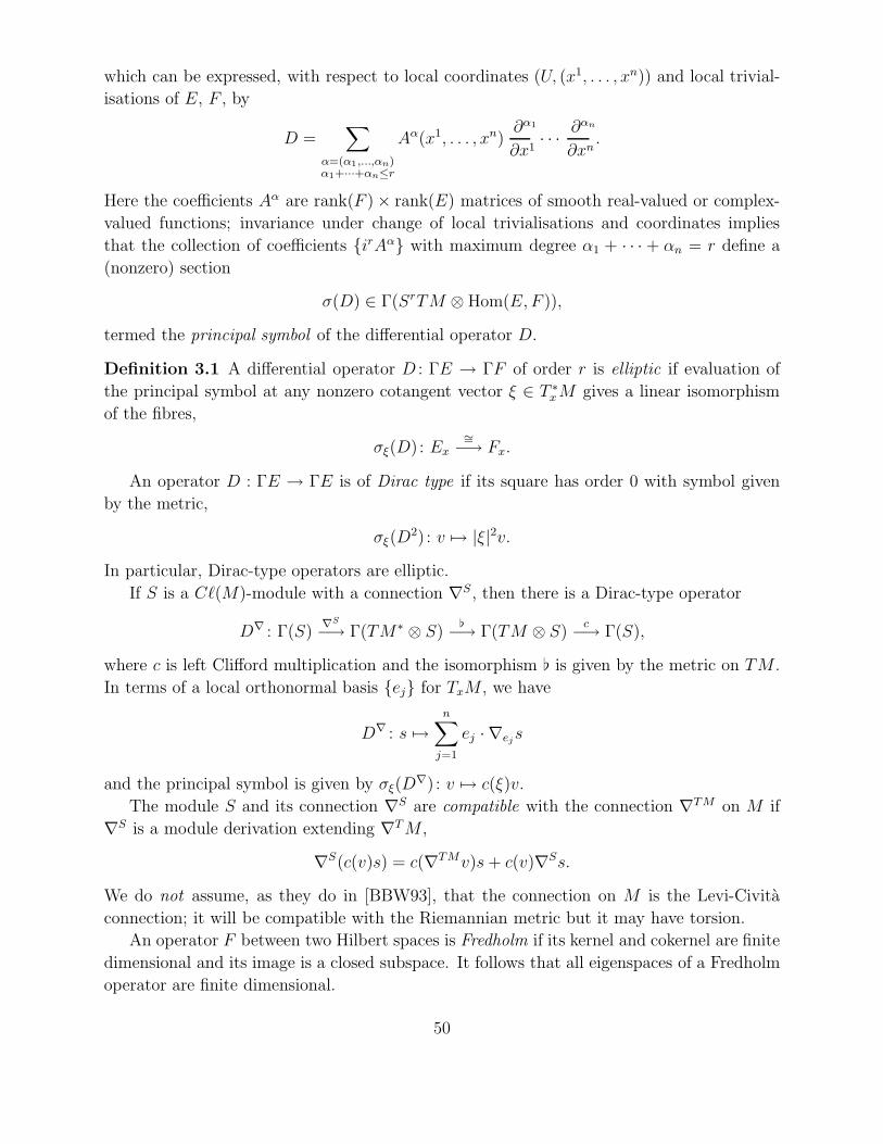
which can be expressed, with respect to local coordinates (U, (x1, . . . , xn)) and local trivial-
isations of E, F , by
D =∑
α=(α1,...,αn)α1+···+αn≤r
Aα(x1, . . . , xn)∂α1
∂x1· · · ∂αn
∂xn.
Here the coefficients Aα are rank(F ) × rank(E) matrices of smooth real-valued or complex-
valued functions; invariance under change of local trivialisations and coordinates implies
that the collection of coefficients irAα with maximum degree α1 + · · · + αn = r define a
(nonzero) section
σ(D) ∈ Γ(SrTM ⊗ Hom(E,F )),
termed the principal symbol of the differential operator D.
Definition 3.1 A differential operator D : ΓE → ΓF of order r is elliptic if evaluation of
the principal symbol at any nonzero cotangent vector ξ ∈ T ∗xM gives a linear isomorphism
of the fibres,
σξ(D) : Ex∼=−→ Fx.
An operator D : ΓE → ΓE is of Dirac type if its square has order 0 with symbol given
by the metric,
σξ(D2) : v → |ξ|2v.
In particular, Dirac-type operators are elliptic.
If S is a C(M)-module with a connection ∇S, then there is a Dirac-type operator
D∇ : Γ(S)∇S−→ Γ(TM∗ ⊗ S)
−→ Γ(TM ⊗ S)c−→ Γ(S),
where c is left Clifford multiplication and the isomorphism is given by the metric on TM .
In terms of a local orthonormal basis ej for TxM , we have
D∇ : s →n∑j=1
ej · ∇ejs
and the principal symbol is given by σξ(D∇) : v → c(ξ)v.
The module S and its connection ∇S are compatible with the connection ∇TM on M if
∇S is a module derivation extending ∇TM ,
∇S(c(v)s) = c(∇TMv)s+ c(v)∇Ss.
We do not assume, as they do in [BBW93], that the connection on M is the Levi-Civita
connection; it will be compatible with the Riemannian metric but it may have torsion.
An operator F between two Hilbert spaces is Fredholm if its kernel and cokernel are finite
dimensional and its image is a closed subspace. It follows that all eigenspaces of a Fredholm
operator are finite dimensional.
50

Lemma 3.2 An elliptic operator P on a compact Riemannian manifold may be completed
to Fredholm operators Ps with respect to the Sobolev norms ‖ ‖s, for which
ker(P ) = ker(Ps), ker(P ∗) = ker(P ∗s ) = coker(Ps)
for all s.
Proof: See Theorem 5.2 in chapter III of [LM89].
For any elliptic operator P : ΓE → ΓF over a compact Riemannian manifold, the compo-
sition of P with its formal adjoint P ∗ gives self-adjoint elliptic operators P ∗P , PP ∗ on ΓE,
ΓF respectively, termed the associated Laplacians of P . Write Eλ, Fλ for the eigenspaces of
these Laplacians for each λ ∈ .
Lemma 3.3 (Hodge) The eigenspaces Eλ, Fλ are finite dimensional and are zero except for
a discrete set of λ ≥ 0. For λ = 0 one has the Hodge formulae
E0 = kerP, F0 = cokerP,
and one has isomorphisms P : Eλ → Fλ for all λ > 0.
3.1.2 The Atiyah–Singer index theorem
The index of an elliptic operator P : ΓE → ΓF may be defined as
ind(P ) = dim ker(P ) − dim coker(P ).
In fact, it depends only on the homotopy class of the principal symbol σ(P ).
The pullback of the principal symbol along π : TM∗ → M is a map
σ(P ) : π∗E → π∗F
which, by the difference bundle construction of Atiyah–Bott–Shapiro [ABS64], defines a
class [σ(P )] ∈ K(DM,SM) in the K-theory of the Thom space of TM . Choosing a smooth
embedding j of M in some N , we now define the topological index of P as the image of the
symbol class [σ(P )] under the composite map
K(DM,SM)∼=−→ Kcpt(TM)
j!−→ Kcpt(TN )
∼=−→ K(S2N )∼=−→ .
Then the Atiyah–Singer index theorem says that the topological index coincides with the
analytic index ind(P ), and may also be expressed in terms of cohomology classes, as follows.
Theorem 3.4 Let M be a compact Riemannian manifold of dimension 4n and P : ΓE → ΓE
a Dirac-type operator on M with coefficients in a vector bundle E. Then
ind(P ) =
∫M
ch(E) A(M),
where A is a polynomial on the Pontrjagin classes of M , and ch(E) is the Chern character
of the bundle E.
51

3.2 The Atiyah–Patodi–Singer theorem
In this chapter we state a version of the Atiyah–Patodi–Singer theorem for manifolds with
boundary and formal operators on infinite-dimensional natural bundles derived from the
tangent bundle.
The interest of this formal construction arises when one shows that the formal sums
involved not only converge but take values in suitable rings of modular forms from elliptic
cohomology, generalising the classical eta invariant.
We state first the classical Atiyah–Patodi–Singer theorem for manifolds with boundary,
under the assumption that the metric near the boundary is of product type. This extends the
theory for closed manifolds by the addition of a term —the eta invariant— whose definition
and properties we review.
Then we recall Gilkey’s modification of the Atiyah–Patodi–Singer formula to include
the case that the metric near the boundary is not of product type. A further integrand now
appears in the formula, which can be expressed in terms of transgression of the characteristic
class involved.
We apply these results for operators arising from elliptic genera on manifolds with bound-
ary, considering both the classical setting and Gilkey’s extension to more general boundary
metrics. We derive expressions for the integrands that arise when generalising from classical
operators to those of elliptic genera.
3.2.1 The classical APS theorem and the eta invariant
Hirzebruch’s signature theorem relates a cohomological invariant, the signature, which may
also be defined as the index of a Dirac-type operator, with an analytical invariant given by
an integral of certain differential forms.
Theorem 3.5 Let M be a 4k-dimensional compact oriented Riemannian manifold. Then
sign(M) = ind(A+) =
∫M
Lk(p1, . . . , pk),
where
• sign(M) is the signature of the non-degenerate intersection form q(a) = (a∪ a)[M ] on
H2k(X;), given by the difference between the number of positive and negative entries
in the diagonalisation of q,
• the signature operator A+ : Ω∗M+ → Ω∗M− is the restriction of A = d+δ = d+∗d∗ to
the ±1 eigenspaces of the involution given by Clifford multiplication by (−1)kω on Ω∗M ,
• the integrand is the Hirzebruch L-polynomial in differential j-forms pj, j = 1, . . . , k,
representing the Pontrjagin classes of M .
52

Proof: The first equality is a straightforward example of Hodge theory. The index of
d+ δ counts the dimensions of harmonic forms in all degrees, but everything cancels except
in the middle dimension, leaving the difference in dimensions of the positive and negative
definite parts. The second equality is the cohomological formula from the Atiyah–Singer
index theorem.
If M is a manifold with boundary ∂M = N , then Atiyah–Patodi–Singer show that an
extra term enters the equation, a new spectral invariant of N , given by a certain number-
theoretic function of the eigenvalues of the signature operator on the boundary.
Definition 3.6 Let A be any endomorphism with a discrete spectrum of eigenvalues λ ∈Spec(A) and finite dimensional eigenspaces. Then the eta function associated to A is given by
ηA(s) =∑λ=0
sign(λ)
|λ|s
where the sum is over the positive and negative eigenvalues, repeated according to their
multiplicities.
Alternatively, one can write
ηA(s) =∑λ>0
dim ker(A− λ)
λs−∑λ<0
dim ker(A− λ)
(−λ)s.
This function will be absolutely convergent for Re(s) sufficiently large. If it has an analytic
continuation such that the value at s = 0 is finite, we write η(A) = ηA(0), the eta invariant
of A.
Theorem 3.7 Let M be a 4k-dimensional compact oriented Riemannian manifold with
boundary N , such that the inclusion N ⊂ M extends to an isometric inclusion in a neigh-
bourhood of the boundary, N × [0, ε] → M . Then
sign(M) = ind(A) + h =
∫M
Lk(p1, . . . , pk) − η(B),
where A the is signature operator as before, and
• sign(M) is now the signature of the non-degenerate quadratic form q′, given by restrict-
ing the intersection form q to the image of H2k(M,N) in H2k(M),
• the differential forms pj represent relative Pontrjagin classes,
• η(B) = ηB(0) is the eta invariant of the self-adjoint operator Bev on the even forms
on N given by
Bevϕ2p = (−1)k+p−1(∗dϕ− d∗ϕ), ϕ ∈ Ω2p(N).
The eta function ηB(s) is holomorphic on the half-plane Re(s) > −12.
53
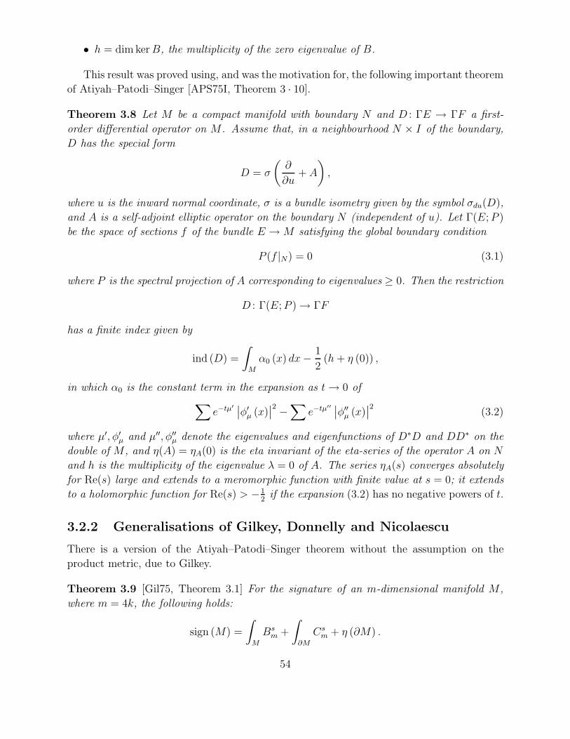
• h = dim kerB, the multiplicity of the zero eigenvalue of B.
This result was proved using, and was the motivation for, the following important theorem
of Atiyah–Patodi–Singer [APS75I, Theorem 3 · 10].
Theorem 3.8 Let M be a compact manifold with boundary N and D : ΓE → ΓF a first-
order differential operator on M . Assume that, in a neighbourhood N × I of the boundary,
D has the special form
D = σ
(∂
∂u+ A
),
where u is the inward normal coordinate, σ is a bundle isometry given by the symbol σdu(D),
and A is a self-adjoint elliptic operator on the boundary N (independent of u). Let Γ(E;P )
be the space of sections f of the bundle E → M satisfying the global boundary condition
P (f |N) = 0 (3.1)
where P is the spectral projection of A corresponding to eigenvalues ≥ 0. Then the restriction
D : Γ(E;P ) → ΓF
has a finite index given by
ind (D) =
∫M
α0 (x) dx− 1
2(h+ η (0)) ,
in which α0 is the constant term in the expansion as t → 0 of∑e−tµ
′ ∣∣φ′µ (x)∣∣2 −
∑e−tµ
′′ ∣∣φ′′µ (x)∣∣2 (3.2)
where µ′, φ′µ and µ′′, φ′′µ denote the eigenvalues and eigenfunctions of D∗D and DD∗ on the
double of M , and η(A) = ηA(0) is the eta invariant of the eta-series of the operator A on N
and h is the multiplicity of the eigenvalue λ = 0 of A. The series ηA(s) converges absolutely
for Re(s) large and extends to a meromorphic function with finite value at s = 0; it extends
to a holomorphic function for Re(s) > −12
if the expansion (3.2) has no negative powers of t.
3.2.2 Generalisations of Gilkey, Donnelly and Nicolaescu
There is a version of the Atiyah–Patodi–Singer theorem without the assumption on the
product metric, due to Gilkey.
Theorem 3.9 [Gil75, Theorem 3.1] For the signature of an m-dimensional manifold M ,
where m = 4k, the following holds:
sign (M) =
∫M
Bsm +
∫∂M
Csm + η (∂M) .
54

More precisely, there is an element TG (Lk) in Pbm−1,m,m−1 such that for any metric on M ,
sign (M) =
∫M
Lk +
∫∂M
TG (Lk) + η (∂M) ,
with
TG (P ) =1
2k
∫ 1
0
P (θ,Ωt, . . . ,Ωt) dt,
θ = ∇1 − ∇0, ∇t = t∇1 + (1 − t) ∇0,
Ωt = Ω∇t ,
so that TG (P ) is an invariantly defined (m − 1)-form with
d (TG (P )) = P (∇1) − P (∇0) .
Fix a Riemannian manifold (M, g), and let T be a tensor (1, 2) on (M, g); that is, a
skew symmetric linear map T : TM × TM → TM , T (Y,X) = −T (X, Y ), and let ∇g,T be
the only metric-compatible connection on M with torsion tensor T . Let dg,T be its skewed
covariant differential, i.e., given by the composition dg,T = ∧ ∇g,T = alt ∇g,T :
C∞ (M,ΛpT ∗M) → C∞ (M,T ∗M ⊗ ΛpT ∗M) → C∞(M,Λp+1T ∗M
).
For T = 0, dg,T = dg,0, the usual exterior derivative associated to the underlying smooth
manifold structure on M .
In general, d and dg,T have the same leading order symbol, but their complete symbols
differ. More precisely, on p-forms,
dg,Tp = dg,0
p + Ep,
where Ep is an endomorphism depending linearly upon the torsion tensor T of ∇g,T.
Consider on the relevant bundles or section spaces the induced metrics and define
δg,T =(dg,T
)∗,
the adjoint of dg,T. Then, on p+ 1 forms, now,
δg,Tp = δg,0
p + E∗p ,
where δg,0p and E∗p are the adjoints for dg,0
p and Ep respectively.
Remark 3.10 Miquel points out [Don86] that for a metric-compatible connection with non-
vanishing torsion T , it is possible that
δg,Tp = ±∗dg,T∗
unlike the Levi-Civita case, in which,
δg,0p = ±∗dg,0∗.
55

For the validity of the classical characteristic class integrands for connections which are
compatible with the metric but have torsion, see Nicolaescu’s approach [Nic99], who refers to
Roe [Roe98, Chapter 11]. However, [Don78] says that, in the case he considers, the integrand
is certainly not the Todd form in general (p. 887) for a Dolbeault operator on a manifold
with boundary.
In manifolds without boundary, they integrate to the same value. There, in fact, thanks
to symbol theory and invariance of characteristic classes with respect to connections and
Stokes, we know that they give the same index.
Hence, since the trace appearing in the Atiyah–Patodi–Singer theorem is a trace on the
double of the manifold, if we know about traces of heat kernels on manifolds without bound-
ary expressed as characteristic forms, we may thereafter restrict them to forms (perhaps not
characteristic but only relatively characteristic in the sense of Kervaire) to obtain results for
the manifolds with boundary.
For the case of manifolds without boundary, all operators can be seen as twisted signature
or twisted Dirac operators.
As an interesting example, consider any compact Lie group, such as for instance the Lie
group as S3 ∼= SU(2). Lie groups are frameable by their Lie algebras and get from there
a natural flat connection with torsion. (E.g., think of any linear group as embedded as an
open set in a general matrix group seen as a flat Euclidean space). However, since this is
not necessarily the Levi-Civita connection (in fact, it would never be so if the Lie algebra
of the group is not trivial) then we can consider equally the other connection. Now, we get
on the Lie group —or, if we prefer, at any compact subspace of it— two metric-compatible
connections, one flat and the other torsion-free. Each connection will have associated a
covariant exterior derivative on differential forms on the Lie group given as the composition
of the connection with the exterior product, which is the same for both. Those operators are
known to share the same leading symbol and hence on manifolds without boundary they will
give the same K-theoretical class. But on manifolds with boundary, they will originate two
different classes both in K and H relative theories. The point is to identify the corresponding
differential forms that one has to integrate.
According to Nicolaescu [Nic99], the formula
ind (Dg ⊗ V ) =
∫M
A(TM,∇g,0
)ch (V ) − 1
2η(Dg⊗V )|∂M
holds in conditions more general than those considered for instance in [BBG89], namely,
ind(Dg,T ⊗ V
)=
∫M
A(TM,∇g,T
)ch (V ) − 1
2η(Dg,T⊗V )|∂M
holds, whenever Dg,T is the Dirac operator associated to the Clifford bundle CnM , but
considered not with the connection induced from the Levi-Civita ∇g,0 on TM , but with any
other one compatible with the metric, probably not torsion free, endowed with a torsion
tensor T . The quoted author says textually that “the proof for (1) in chapter eleven of
56

Roe’s book, edition 88, extends verbatim to (2).” We will prove the truth of this statement,
beginning from [Roe98, p. 136].
We will begin by considering M a spin manifold of even dimension n. We know that
M has a canonical Clifford bundle S over it, whose fibre is the spin representation ρS , and
associated to S there is a Dirac operator D = c ∇g,0, which is a graded one. However, we
are not interested on this D only, which is what we called Dg,0. We want to consider further
operators
Dg,T = c ∇g,T .
Lemma 11.30 in [Roe98] (referring to the case of spin even-dimensional manifolds without
boundary) says that the signature operator is canonically isomorphic to the classical Dirac
operator with coefficients in the spin bundle S. Since, as left Clifford modules,
Λ∗ (T ∗M) ⊗ ∼= Cn (T ∗M ⊗ ) ∼= S ⊗ S,
and since the first order parts of both considered operators agree under this isomorphism,
their difference must be a zeroth order (tensorial) operator, which depends on the connection
coefficients in a linear way. For the classical versions considered by Roe, being the connection
on TM Riemannian, it is possible, once fixed any point x, to take normal coordinates centred
there, so that the components of the connection vanish there, and hence in the classical case
the difference must be zero.
3.2.3 Eta invariants of twisted Dirac operators
Let M be an oriented compact Riemannian manifold of dimension 2n, such that the Rieman-
nian metric coincides in a neighbourhood of the boundary N = ∂M with a product metric
on N × I. Suppose that M is a spin manifold. Then the Dirac operator of M is a first order
elliptic differential operator on the graded spinor bundles,
D+ : ΓS+ → ΓS− .
On the boundary, S± restrict to give the spinor bundle associated to N , and in a neighbour-
hood of the boundary one has
D+ = σ
(∂
∂u+ A
),
where σ is Clifford multiplication by the unit inward normal as usual, and DN is just the
Dirac operator on the (2n − 1)-manifold N . In [ABP73], Atiyah–Bott–Patodi show that
the integrand α0(x) dx in Theorem 3.8 can be expressed explicitly as an appropriate Pontr-
jagin form in this case and that the corresponding expansion (3.2) has no negative powers
of t, and one obtains a formula for the index of Dirac operator with the global boundary
condition (3.1).
Atiyah–Patodi–Singer themselves point out that the results of [ABP73, Section 6] also
apply to twisted Dirac operators:
57

Theorem 3.11 Suppose E is a hermitian vector bundle on M with a unitary connection
such that near the boundary the metric and the connection are constant in the normal direc-
tion. Then the twisted Dirac operator on M ,
D+E : Γ(S+ ⊗ E) → Γ(S− ⊗ E)
with the global boundary condition (3.1) has index
ind(D+E) =
∫M
ch(E) A(p) − 1
2(hE|N + ηE|N),
where A(p) is the Hirzebruch A-polynomialn∏i=1
xi/2
sinh(xi/2)with the elementary symmetric
functions of the x2i replaced by Pontrjagin forms on M , the form ch(E) denotes the Chern
character of the bundle, ηE|N(s) is the eta-function of the twisted Dirac operator on N and
hE|N is the dimension of its kernel. Moreover, η(s) is holomorphic for Re(s) > −12.
Theorem 3.7 is a version of this, although M is not required to be spin and the factor
of 12
is present only implicitly, since the operator B on the even forms is only ‘half’ of the
restriction A|∂M of the signature operator.
We can generalise the previous theorem in a purely formal way to graded bundles or
q-bundles. Suppose that Er, r ≥ 0, is a sequence of vector bundles as above. We usually
write
Eq =⊕r≥0
Er qr.
Here q is simply a formal variable. The formal bundle Eq may be of infinite rank, but each
Er will always be of finite rank. Then the Dirac operator on M may be twisted with Eq.
If we write D+r for the twisted Dirac operator D+
Erthen we have
D+q =
∑r≥0
D+r q
r : Γ(S+ ⊗Eq) → Γ(S− ⊗ Eq).
The index of D+q is the formal power series
ind(D+q ) =
∑r≥0
ind(D+r ) qr =
∑r≥0
(dim ker(D+
r ) − dim coker(D+r ))qr.
The operators D+r , D+
q restricted to the boundary of M give the twisted Dirac operators
Dr,N and
Dq,N =∑r
Dr,N qr
on N . We consider the corresponding eta invariants, as follows.
58

Definition 3.12 The eta function of a twisted Dirac operator Dq is the formal series
ηDq(s, q) =∑r≥0
ηDr(s) qr.
If each eta function ηDr(s) has finite value at s = 0 then the eta invariant of Dq is the formal
power series
ηDq(q) =∑r≥0
η(Dr) qr.
One considers similarly the formal power series
h(q) = dim ker(Dq) =∑r≥0
dim ker(Dr) qr
and the formal Chern character
ch(Eq) =∑r≥0
ch(Er) qr .
Corollary 3.13 The formal twisted Dirac operator D+q with the global boundary condition
(3.1) has index
ind(D+q ) =
∫M
ch(Eq)(q) A(p) − hDq,N(q) + ηDq,N
(q)
2,
Proof: Apply the previous theorem to each twisted Dirac operator D+r and add up.
3.2.4 Eta invariants of twisted signature operators
The signature operator A+ : Ω∗M+ → Ω∗M− may also be generalised to a twisted operator,
as follows. Let E be a hermitian vector bundle, with a compatible connection ∇E, over a
compact Riemannian manifold of dimension 2n. Consider the covariant exterior derivative
dE = d∇ on Ω∗(M ;E), the space of differential forms on M with coefficients in the bundle E.
As for the usual exterior coderivative, the adjoint δE = d∗E is given by
δE = ±∗dE∗,
where the Hodge star acts as the identity on the coefficients. It follows that the self-adjoint
operator AE = dE + δE splits as
A±E : Ω±(M ;E) → Ω∓(M ;E), Ω±(M ;E) = (1 ± inω)Ω(M ;E).
The operator A+E is the twisted signature operator, and one has a generalised Hirzebruch
signature theorem:
59

Theorem 3.14 Let sign(M ;E) be the signature of the quadratic form given by wedge product
on Hn(M ;E). Then
sign(M ;E) = ind(A+E) = 2nch(E) L(M)[M ],
where L denotes the Hirzebruch characteristic class
n∏i=1
xi/2
tanh(xi/2)with the elementary sym-
metric functions of the x2i replaced by Pontrjagin classes of M .
Proof: This is completely parallel to the usual Signature Theorem 3.5; see [ABP73, p. 313]
for more details.
We can also take E to be a graded vector bundle Eq =⊕
Erqr as discussed above, and
we will then interpret the twisted signature theorem as giving equality of power series in the
formal variable q. The main example is given by the graded bundle LEq, defined as follows.
Let E be any vector bundle over M , and define
LEq =∞⊗j=1
SqjE ⊗∞⊗j=1
ΛqjE,
where we use the notation St, Λt for the formal power series versions of the symmetric and
exterior products S∗, Λ∗. Explicitly, we set
StE =
∞∑=0
S(E) · t, ΛtE =
∞∑=0
Λ(E) · t.
In the case of the complex tangent bundle E = TM = TM ⊗ , we sometimes write LM =
LTMq. This bundle is termed the free loop bundle on M and the corresponding twisted
signature is usually interpreted as the S1-equivariant signature of the free loop space LM ,
signS1
(M) = sign(M ; LM) =∑r≥0
sign(M ; LTMr) qr.
Corollary 3.15 The S1-equivariant signature is related to the universal elliptic genus by
signS1
(M4k) εk/2 = ϕE(M4k).
Proof: The Chern character of StE is just∏n
i=1
∑k≥0 t
kekxi =∏n
i=1(1−texi)−1 and similarly
ch(LM) =
n∏i=1
∞∏j=1
(1 + qnexi)(1 + qne−xi)
(1 − qnexi)(1 − qne−xi).
The result follows from Theorem 3.14 on comparing with the characteristic class for the
universal elliptic genus; compare [HBJ92, Theorem I.5.6 and Section 6.1].
60
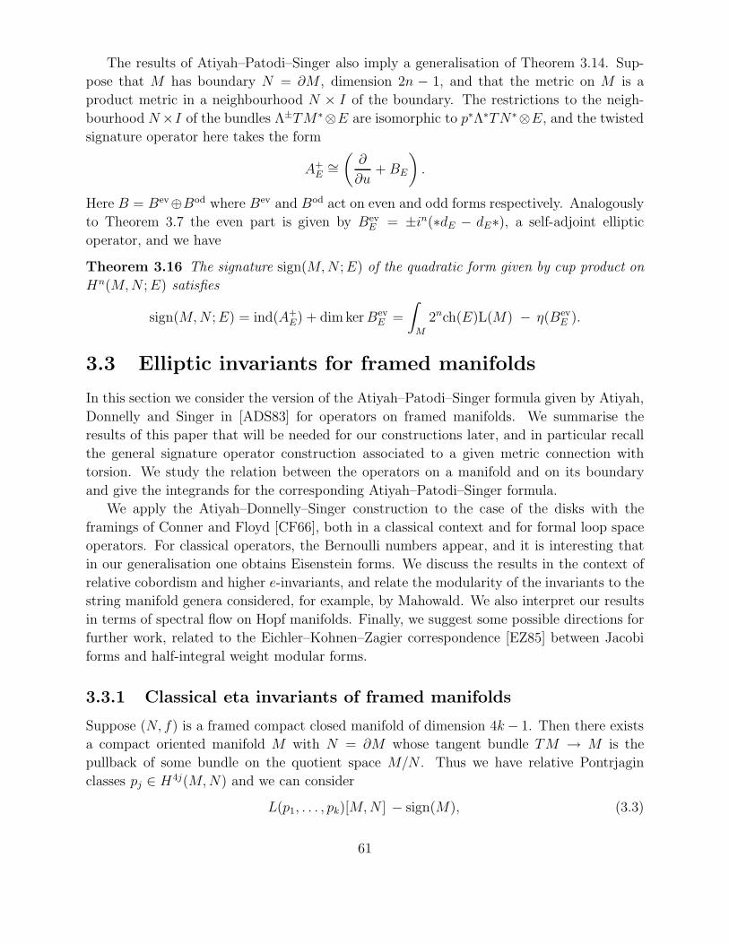
The results of Atiyah–Patodi–Singer also imply a generalisation of Theorem 3.14. Sup-
pose that M has boundary N = ∂M , dimension 2n − 1, and that the metric on M is a
product metric in a neighbourhood N × I of the boundary. The restrictions to the neigh-
bourhood N×I of the bundles Λ±TM∗⊗E are isomorphic to p∗Λ∗TN∗⊗E, and the twisted
signature operator here takes the form
A+E
∼=(∂
∂u+BE
).
Here B = Bev ⊕Bod where Bev and Bod act on even and odd forms respectively. Analogously
to Theorem 3.7 the even part is given by BevE = ±in(∗dE − dE∗), a self-adjoint elliptic
operator, and we have
Theorem 3.16 The signature sign(M,N ;E) of the quadratic form given by cup product on
Hn(M,N ;E) satisfies
sign(M,N ;E) = ind(A+E) + dim kerBev
E =
∫M
2nch(E)L(M) − η(BevE ).
3.3 Elliptic invariants for framed manifolds
In this section we consider the version of the Atiyah–Patodi–Singer formula given by Atiyah,
Donnelly and Singer in [ADS83] for operators on framed manifolds. We summarise the
results of this paper that will be needed for our constructions later, and in particular recall
the general signature operator construction associated to a given metric connection with
torsion. We study the relation between the operators on a manifold and on its boundary
and give the integrands for the corresponding Atiyah–Patodi–Singer formula.
We apply the Atiyah–Donnelly–Singer construction to the case of the disks with the
framings of Conner and Floyd [CF66], both in a classical context and for formal loop space
operators. For classical operators, the Bernoulli numbers appear, and it is interesting that
in our generalisation one obtains Eisenstein forms. We discuss the results in the context of
relative cobordism and higher e-invariants, and relate the modularity of the invariants to the
string manifold genera considered, for example, by Mahowald. We also interpret our results
in terms of spectral flow on Hopf manifolds. Finally, we suggest some possible directions for
further work, related to the Eichler–Kohnen–Zagier correspondence [EZ85] between Jacobi
forms and half-integral weight modular forms.
3.3.1 Classical eta invariants of framed manifolds
Suppose (N, f) is a framed compact closed manifold of dimension 4k− 1. Then there exists
a compact oriented manifold M with N = ∂M whose tangent bundle TM → M is the
pullback of some bundle on the quotient space M/N . Thus we have relative Pontrjagin
classes pj ∈ H4j(M,N) and we can consider
L(p1, . . . , pk)[M,N ] − sign(M), (3.3)
61
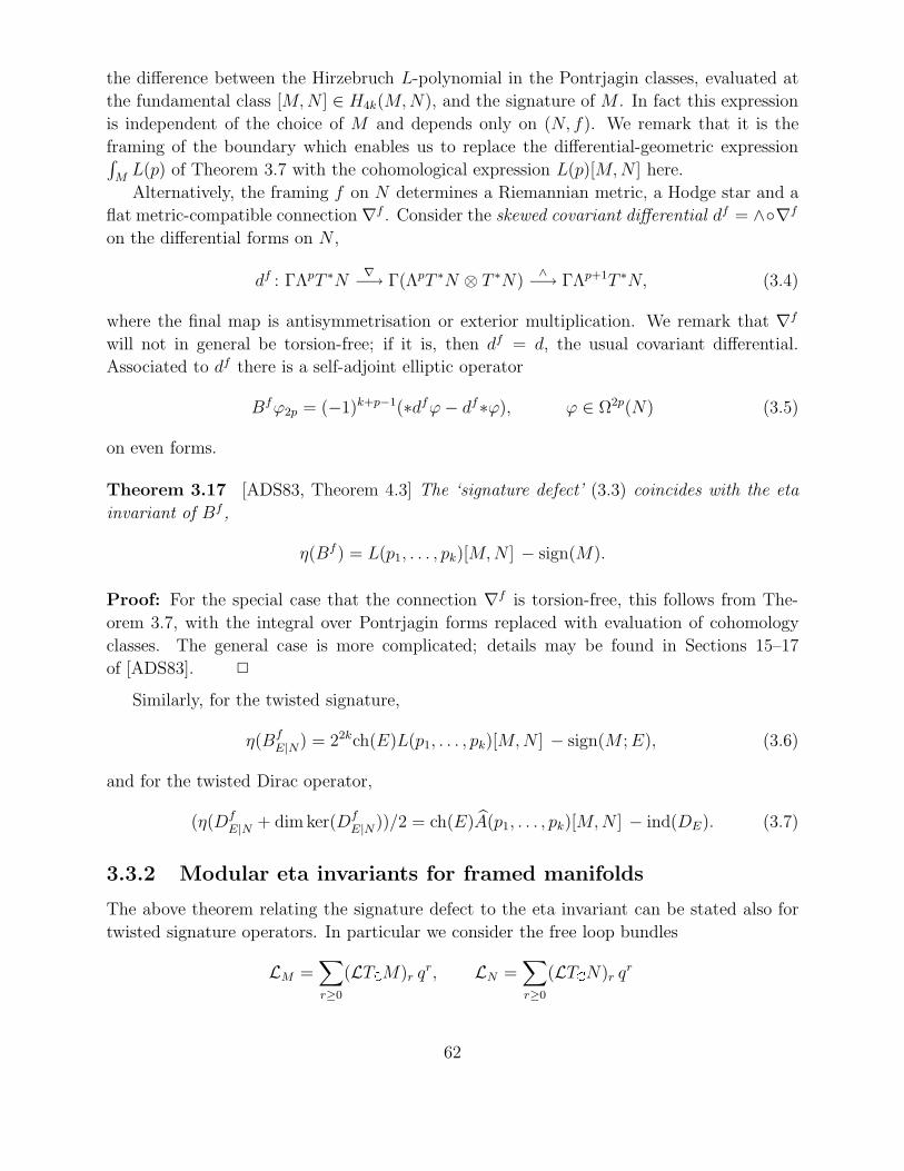
the difference between the Hirzebruch L-polynomial in the Pontrjagin classes, evaluated at
the fundamental class [M,N ] ∈ H4k(M,N), and the signature of M . In fact this expression
is independent of the choice of M and depends only on (N, f). We remark that it is the
framing of the boundary which enables us to replace the differential-geometric expression∫ML(p) of Theorem 3.7 with the cohomological expression L(p)[M,N ] here.
Alternatively, the framing f on N determines a Riemannian metric, a Hodge star and a
flat metric-compatible connection ∇f . Consider the skewed covariant differential df = ∧∇f
on the differential forms on N ,
df : ΓΛpT ∗N ∇−→ Γ(ΛpT ∗N ⊗ T ∗N)∧−→ ΓΛp+1T ∗N, (3.4)
where the final map is antisymmetrisation or exterior multiplication. We remark that ∇f
will not in general be torsion-free; if it is, then df = d, the usual covariant differential.
Associated to df there is a self-adjoint elliptic operator
Bfϕ2p = (−1)k+p−1(∗dfϕ− df∗ϕ), ϕ ∈ Ω2p(N) (3.5)
on even forms.
Theorem 3.17 [ADS83, Theorem 4.3] The ‘signature defect’ (3.3) coincides with the eta
invariant of Bf ,
η(Bf) = L(p1, . . . , pk)[M,N ] − sign(M).
Proof: For the special case that the connection ∇f is torsion-free, this follows from The-
orem 3.7, with the integral over Pontrjagin forms replaced with evaluation of cohomology
classes. The general case is more complicated; details may be found in Sections 15–17
of [ADS83].
Similarly, for the twisted signature,
η(BfE|N) = 22kch(E)L(p1, . . . , pk)[M,N ] − sign(M ;E), (3.6)
and for the twisted Dirac operator,
(η(DfE|N + dim ker(Df
E|N))/2 = ch(E)A(p1, . . . , pk)[M,N ] − ind(DE). (3.7)
3.3.2 Modular eta invariants for framed manifolds
The above theorem relating the signature defect to the eta invariant can be stated also for
twisted signature operators. In particular we consider the free loop bundles
LM =∑r≥0
(LTM)r qr, LN =
∑r≥0
(LTN)r qr
62

which inherit flat connections from the tangent bundles and we can consider the formal
covariant exterior derivative dfLNon Ω∗(N ; LN ) with
dfLN=
∑r≥0
dfLTNrqr : Ωk(N ; LTNr) → Ωk+1(N ; LTNr).
Then we have operators BfLTNr
= ±(∗dfLTNr− dfLTNr
∗) as before and a formal operator
BfLN
=∑BfLTNr
qr on the even forms on N with coefficients in the free loop bundle on the
loop space.
Definition 3.18 Let M be an oriented manifold of dimension 4k with framed boundary
(N, f) of dimension 4k− 1. Then the relative S1-equivariant signature of the free loop space
is given by the signature of the cup product in relative cohomology with coefficients in the
free loop bundle LM ,
signS1
(M,N) = sign(M,N ; LM) =∑r≥0
sign(M,N ; LTMr) qr ∈ [[q]].
The elliptic eta invariant of the framed manifold (N, f) is the formal power series
ηE(N, f) =∑r≥0
η(BfLTMr
) qr ∈ [[q]]
given by the eta invariants for the twisted operators BfLTNr
on Ωev(N ; LTNr).
We then have an elliptic cohomology generalisation of the Signature Defect Theorem 3.17:
Theorem 3.19 The relative universal elliptic genus of a framed (4k − 1)-manifold satisfies
ηE(N, f) = ϕE(M,N) ε−k/2 − signS1
(M,N).
Proof: Define the relative universal elliptic genus of (N, f), and apply (3.6) to each term in
the q-expansions (see [HBJ92, 6.1]).
Corollary 3.20 The following relation holds in (/)[[q]]:
ηE(N, f) ≡ ϕE(M,N) ε−k/2 (mod ) .
Corollary 3.21 If the S1-signature vanishes, then
ηE(N, f) = ϕE(M,N) ε−k/2 .
If, in addition, k is even, then the elliptic eta invariant is a modular function of weight zero
for the congruence subgroup Γ0(2).
63

Similar results hold for the Dirac operator on spin manifolds twisted by Sq =∑SrTM ,
corresponding to the Witten genus rather than the elliptic genus.
We give an example of Corollary 3.21 for the case that N is the sphere. The beauty of
this example is the relation between the elliptic eta invariant and the Eisenstein series used
in the definition of the universal elliptic genus.
Proposition 3.22 There is a framing f of the boundary S4k−1 of the disk D4k for which
the elliptic eta invariant is given by
ηE(N, f) =4G∗2kεk/2
.
Proof: First note that the signature and relative signature of the disk D4k are zero, since it
has zero cohomology in dimension 2k. This is true for any twisted signature with coefficients
in a flat bundle and for the S1-signature of the free loop space. Thus we are in the situation
of Corollary 3.21 and we have
ηE(N, f) =ϕE(D4k, S4k−1)
εk/2.
Now recall [Smi71], [CF66] that a framing f may be chosen for the boundary such that
ci =
0 for 0 ≤ i < 2k ,
(2k − 1)! for i = 2k .
Since all but the highest Chern class vanish, the genus will be c2k ·a2k, where the characteristic
series has the form P (u) = exp(∑−a2ku
2k/2k)
(see [HBJ92, p. 20] for details). For the
universal elliptic genus, then, we have
ϕE(D4k, S4k−1) = (2k − 1)! (−2k)4G∗2k(τ)(2k)!
= −4G∗2k,
as claimed.
We will need to consider the reduction modulo Z of the above invariants, where Z is one
of the rings , [12], or more generally [ 1
n] or [ 1
2n] for n odd. Recall the elliptic genus ϕε
takes as values homogeneous polynomials in [δ, ε], where δ, ε have degree 2, 4 respectively,
and so the normalised elliptic genus ϕε(M4k) = ϕε(M)/εk/2 is a polynomial in
ρ = δ/√ε = 1 + 32q + 256q2 + 1408q3 + 6144q4 + 22976q5 + · · ·
taking the q-expansion at the signature cusp i∞. In fact ρ ∈ 1 + 32[q]; in terms of the
Dedekind eta function,
ρ− 1 = 32η (4τ)8
η (τ)8 = 32q
( ∞∏n=1
(1 − q4n
1 − qn
))
= 32q
( ∞∏n=1
(1 + qn + q2n + q3n
))
64
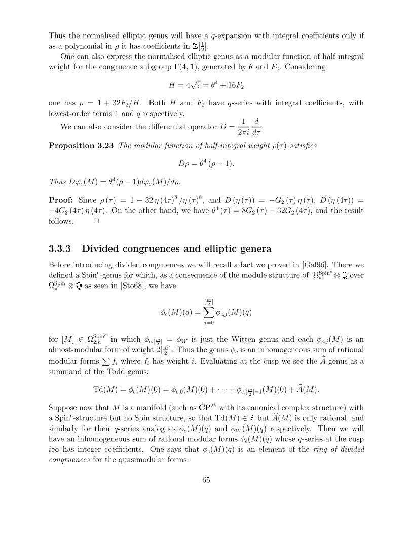
Thus the normalised elliptic genus will have a q-expansion with integral coefficients only if
as a polynomial in ρ it has coefficients in [12].
One can also express the normalised elliptic genus as a modular function of half-integral
weight for the congruence subgroup Γ(4, 1), generated by θ and F2. Considering
H = 4√ε = θ4 + 16F2
one has ρ = 1 + 32F2/H . Both H and F2 have q-series with integral coefficients, with
lowest-order terms 1 and q respectively.
We can also consider the differential operator D =1
2πi
d
dτ.
Proposition 3.23 The modular function of half-integral weight ρ(τ) satisfies
Dρ = θ4 (ρ− 1).
Thus Dϕε(M) = θ4(ρ− 1)dϕε(M)/dρ.
Proof: Since ρ (τ) = 1 − 32 η (4τ)8 /η (τ)8, and D (η (τ)) = −G2 (τ) η (τ), D (η (4τ)) =
−4G2 (4τ) η (4τ). On the other hand, we have θ4 (τ) = 8G2 (τ) − 32G2 (4τ), and the result
follows.
3.3.3 Divided congruences and elliptic genera
Before introducing divided congruences we will recall a fact we proved in [Gal96]. There we
defined a Spinc-genus for which, as a consequence of the module structure of ΩSpinc
∗ ⊗ over
ΩSpin∗ ⊗ as seen in [Sto68], we have
φc(M)(q) =
[ m2
]∑j=0
φc,j(M)(q)
for [M ] ∈ ΩSpinc
2m in which φc,[ m2
] = φW is just the Witten genus and each φc,j(M) is an
almost-modular form of weight 2[m2]. Thus the genus φc is an inhomogeneous sum of rational
modular forms∑fi where fi has weight i. Evaluating at the cusp we see the A-genus as a
summand of the Todd genus:
Td(M) = φc(M)(0) = φc,0(M)(0) + · · · + φc,[ m2
]−1(M)(0) + A(M).
Suppose now that M is a manifold (such as CP2k with its canonical complex structure) with
a Spinc-structure but no Spin structure, so that Td(M) ∈ but A(M) is only rational, and
similarly for their q-series analogues φc(M)(q) and φW (M)(q) respectively. Then we will
have an inhomogeneous sum of rational modular forms φc(M)(q) whose q-series at the cusp
i∞ has integer coefficients. One says that φc(M)(q) is an element of the ring of divided
congruences for the quasimodular forms.
65

In general, following Katz [Kat75] and using the notation of Laures [Lau99], we define
the ring of divided congruences associated to a congruence subgroup Γ as the ring of inho-
mogeneous rational modular forms∑fi where fi has is a form of weight i for γ, such that
for each integer k = 0 the q-expansion of the sum∑k−ifi at any cusp has coefficients in
Γ[ 1k], where Γ = π(KΓ).
Theorem 3.24 (Clarke–Johnson) Let D denote the ring of non-homogeneous sums of ra-
tional modular forms for Γ0 (2) such that the q-series of the sum is in [12][[q]]. Then
KO0 (E) ∼= D[∆−1]
where E = [δ, ε][12][∆−1].
Theorem 3.25 Let ϕ be any Hirzebruch genus of elliptic type for a ring of modular forms
fulfilling the hypotesis of the Katz theorem. Then the following facts hold:
1. The generators for the ring of divided congruences cn are determined by
∞∑n=1
log
(1
1 − cnyn
)=
∞∑m≥1
ϕ ( Pm)
m+ 1ym+1 = gϕ (τ, y)
so that
ϕ (Pn) =∑d|n
cn/dn · d.
2. Let Lϕ (x) = log (Qϕ (τ, x)), whose Taylor expansion in x is
log (Qϕ (τ, x)) =
∞∑m≥1
ϕ(D4k, S4k−1, π
)(2k)!
x2k
for(D4k, S4k−1, π
)the framed disks defined above. Then ϕ
(D4k, S4k−1, π
)generate the
image of ΩG(Eϕ)∗ up to 2-torsion and writing Gϕ
2k1= ϕ
(D4k, S4k−1, π
)for the Eisenstein
series determined by the genus ϕ we have
ϕE( P2k ) =∑Pk
1
r1! · · · rt!(Gϕ
2k1)r1 · · · (Gϕ
2kt)rt
kr11 · · · krtt (2k1 − 1)!r1 · · · (2kt − 1)!rt(2k + 1)t
where the summation is over partitions k =∑rjkj, rj ≥ 1 and 0 < kj < kj+1.
Whenever we have an elliptic genus, determined by its logarithm gϕ (τ, y), we see that
the Katz divided congruences definitions may be written as
∞∏n=1
(1 − cnyn)−1 =
∞∑n=0
bnyn = exp(gϕ(τ, y)).
66

Observe moreover that for any genus ϕE corresponding to a suitably oriented generalized
cohomology theory Eϕ by a class xEϕ we have
gϕ (τ, y) = gϕ(τ, xEϕ
)= xH
where xH denotes the usual oriented cohomology oriented with genus given by the additive
formal group law. Then the expressions above become
∞∏n=1
(1 − cn
(xEϕ
)n)−1=∞∑n=0
bn(xEϕ)n = exp(gϕ(τ, x
Eϕ))
and, since the orientation for the multiplicative group law in K-theory is given under the
orientation provided by the Todd genus ϕTd, by
gϕTd(τ, y) = gϕTd
(τ, xK) = xH = log
(1
1 − xK
).
Now suppose we are using the elliptic cohomology theory considered by Devoto, with
Miller’s character, composed with complexification, so that
Θ(τ, xK
)= xEϕ .
Then the image of the K-theoretical orientation class and the Katz series b are related via(b−1)( 1
1 − xK
)= xEϕ = Θ
(τ, xK
).
3.4 Equivariant elliptic invariants
We now examine the constructions of the previous section for operators on manifolds with a
(finite) group action. First we summarise the results of Donnelly [Don78] for the equivariant
Atiyah–Patodi–Singer formula for manifolds with group actions, and recall the definition of
the classical Atiyah–Singer invariants from [AB66, AS68I]. We generalise these results to
cover the case of Dirac operators associated to elliptic genera, acting on framed manifolds.
We compute the resulting invariants for the classical lens spaces and show that they
are precisely the level-two modular functions which generate the coefficient ring of Devoto’s
equivariant elliptic cohomology [Dev96b].
Let Y be an odd-dimensional spin manifold of dimension 4k − 1 with finite fundamental
group π1Y = G of odd order and let E → Y be a unitary flat bundle of dimension m
associated to a representation
α : G → U(m)
of G. We may denote E by Eα when we want to emphasise this relationship between the
bundle and the representation.
67

We assume a Riemannian metric and connection are given on Y and that G acts by
orientation-preserving isometries, and we may consider
G → Isom+ (Y ) .
We give the bundle the usual flat connection. Suppose further that Y bounds some 4k-
dimensional manifold X and that E extends to a bundle W over X, which may not be
flat.
We will construct the R-class of the manifold X associated to the representation α,
Rq,α(TX) ∈ K∗∗(X)[[q]],
as follows. Recall the loop signature class Rq =⊕
Rnqn for the bundle W by
Rq(W ) =⊕n≥0
Rn(W )qn =∞⊗n=1
SqnW ⊗∞⊗n=1
ΛqnW.
We remark that all the bundles Rn(W ) inherit a flat connection. We shall write αn for the
unitary representation of π1Y which gives Rn(E). Let mn denote the dimension of Rn(E).
We also have a loop signature class for the tangent bundle,
Rq(TX) =⊕n≥0
Rn(TX)qn =∞⊗n=1
Sqn(TX ⊗ ) ⊗∞⊗n=1
Λqn(TX ⊗ ).
We shall define a formal power series of bundles by
Rq,α(TX) =∑n≥0
Rn,α(TX)qn = Rq(TX) ⊗ Rq(W ).
Each summand Rn,α(TX) can be written in the form
Rn,α(TX) =∑m
Rn,αn−m(TX)
=∑m
Rm(TX) ⊗Rn−m(W ).
Adding all of them up we get a (formal, virtual) bundle over X that we may denote by
Rq,α (TX). Let DRq,α(TX)+ denote the signature operator on X twisted by the bundle Rq (TX)
with respect to the representation α. We shall define DRq(TX)+,n as the Dirac operator twisted
by Rn (TX).
For every twisted signature operator Dξ+ we may consider
Definition 3.26 The eta invariant for the operator Dξ+ is
ηDξ+
(s) =∑
λ=0, λ∈Spec(Dξ+)
sign (λ)
|λ|s .
68
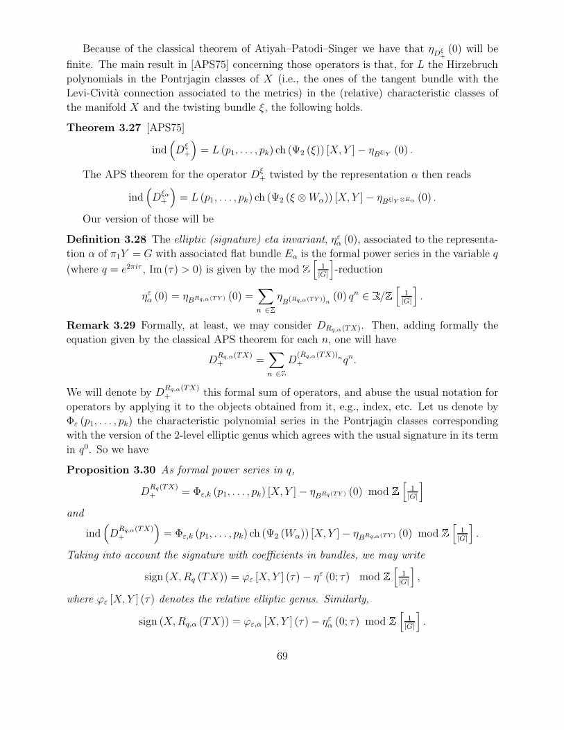
Because of the classical theorem of Atiyah–Patodi–Singer we have that ηDξ+
(0) will be
finite. The main result in [APS75] concerning those operators is that, for L the Hirzebruch
polynomials in the Pontrjagin classes of X (i.e., the ones of the tangent bundle with the
Levi-Civita connection associated to the metrics) in the (relative) characteristic classes of
the manifold X and the twisting bundle ξ, the following holds.
Theorem 3.27 [APS75]
ind(Dξ
+
)= L (p1, . . . , pk) ch (Ψ2 (ξ)) [X, Y ] − ηBξ|Y (0) .
The APS theorem for the operator Dξ+ twisted by the representation α then reads
ind(Dξα
+
)= L (p1, . . . , pk) ch (Ψ2 (ξ ⊗Wα)) [X, Y ] − ηBξ|Y ⊗Eα (0) .
Our version of those will be
Definition 3.28 The elliptic (signature) eta invariant, ηεα (0), associated to the representa-
tion α of π1Y = G with associated flat bundle Eα is the formal power series in the variable q
(where q = e2πiτ , Im (τ) > 0) is given by the mod [
1|G|
]-reduction
ηεα (0) = ηBRq,α(TY ) (0) =∑n ∈
ηB(Rq,α(TY ))n
(0) qn ∈ /[
1|G|
].
Remark 3.29 Formally, at least, we may consider DRq,α(TX). Then, adding formally the
equation given by the classical APS theorem for each n, one will have
DRq,α(TX)+ =
∑n ∈
D(Rq,α(TX))n+ qn.
We will denote by DRq,α(TX)+ this formal sum of operators, and abuse the usual notation for
operators by applying it to the objects obtained from it, e.g., index, etc. Let us denote by
Φε (p1, . . . , pk) the characteristic polynomial series in the Pontrjagin classes corresponding
with the version of the 2-level elliptic genus which agrees with the usual signature in its term
in q0. So we have
Proposition 3.30 As formal power series in q,
DRq(TX)+ = Φε,k (p1, . . . , pk) [X, Y ] − ηBRq(TY ) (0) mod
[1|G|
]and
ind(DRq,α(TX)+
)= Φε,k (p1, . . . , pk) ch (Ψ2 (Wα)) [X, Y ] − ηBRq,α(TY ) (0) mod
[1|G|
].
Taking into account the signature with coefficients in bundles, we may write
sign (X,Rq (TX)) = ϕε [X, Y ] (τ) − ηε (0; τ) mod [
1|G|
],
where ϕε [X, Y ] (τ) denotes the relative elliptic genus. Similarly,
sign (X,Rq,α (TX)) = ϕε,α [X, Y ] (τ) − ηεα (0; τ) mod [
1|G|
].
69
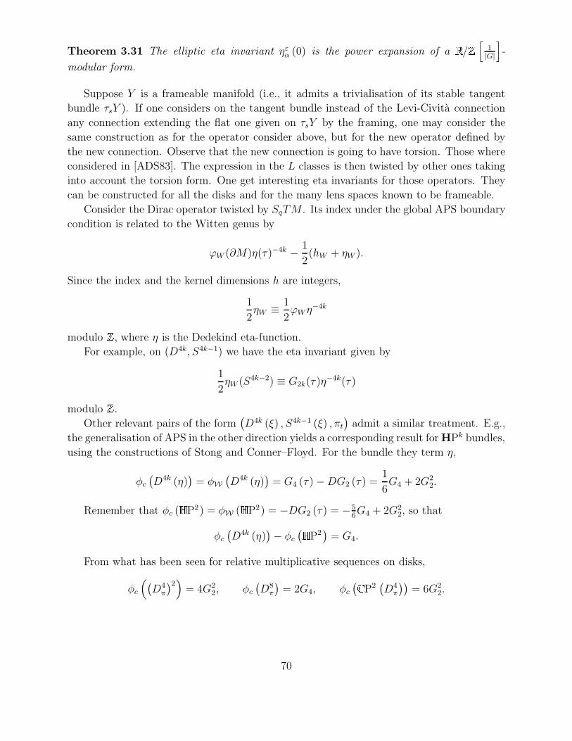
Theorem 3.31 The elliptic eta invariant ηεα (0) is the power expansion of a /[
1|G|
]-
modular form.
Suppose Y is a frameable manifold (i.e., it admits a trivialisation of its stable tangent
bundle τsY ). If one considers on the tangent bundle instead of the Levi-Civita connection
any connection extending the flat one given on τsY by the framing, one may consider the
same construction as for the operator consider above, but for the new operator defined by
the new connection. Observe that the new connection is going to have torsion. Those where
considered in [ADS83]. The expression in the L classes is then twisted by other ones taking
into account the torsion form. One get interesting eta invariants for those operators. They
can be constructed for all the disks and for the many lens spaces known to be frameable.
Consider the Dirac operator twisted by SqTM . Its index under the global APS boundary
condition is related to the Witten genus by
ϕW (∂M)η(τ)−4k − 1
2(hW + ηW ).
Since the index and the kernel dimensions h are integers,
1
2ηW ≡ 1
2ϕWη
−4k
modulo , where η is the Dedekind eta-function.
For example, on (D4k, S4k−1) we have the eta invariant given by
1
2ηW (S4k−2) ≡ G2k(τ)η
−4k(τ)
modulo .
Other relevant pairs of the form(D4k (ξ) , S4k−1 (ξ) , πt
)admit a similar treatment. E.g.,
the generalisation of APS in the other direction yields a corresponding result for HPk bundles,
using the constructions of Stong and Conner–Floyd. For the bundle they term η,
φc(D4k (η)
)= φW
(D4k (η)
)= G4 (τ) −DG2 (τ) =
1
6G4 + 2G2
2.
Remember that φc ( P2) = φW ( P2) = −DG2 (τ) = −56G4 + 2G2
2, so that
φc(D4k (η)
)− φc( P2
)= G4.
From what has been seen for relative multiplicative sequences on disks,
φc
((D4π
)2)= 4G2
2, φc(D8π
)= 2G4, φc
( P2
(D4π
))= 6G2
2.
70