MODIS VEGETATION INDEX(MOD 13)

ALGORITHM THEORETICAL BASISDOCUMENT

Version 3

Alfredo Huete1

Chris Justice2

(Team Members)

and

Wim van Leeuwen1

(Associate Team Member)

11200 E. South Campus Drive429 Shantz Bldg. #38University of Arizona

Tucson, Arizona 85721ahuete@ag.arizona.edu

leeuw@ag.arizona.edu

2University of VirginiaDepartment of Environmental Sciences

Clark HallCharlottesville, VA 22903

justice@virginia.edu

April 30, 1999

i

EXECUTIVE SUMMARY

One of the primary interests of the Earth Observing System (EOS) program is tostudy the role of terrestrial vegetation in large-scale global processes with the goal ofunderstanding how the Earth functions as a system. This requires an understanding ofthe global distribution of vegetation types as well as their biophysical and structuralproperties and spatial/temporal variations. Vegetation Indices (VI) are robust, empiricalmeasures of vegetation activity at the land surface. They are designed to enhance thevegetation signal from measured spectral responses by combining two (or more)different wavebands, often in the red (0.6-0.7 µm) and NIR wavelengths (0.7-1.1 µm).

The MODIS vegetation index (VI) products will provide consistent, spatial andtemporal comparisons of global vegetation conditions which will be used to monitor theEarth's terrestrial photosynthetic vegetation activity in support of phenologic, changedetection, and biophysical interpretations. Gridded vegetation index maps depictingspatial and temporal variations in vegetation activity are derived at 16-day and monthlyintervals for precise seasonal and interannual monitoring of the Earth’s vegetation.

The MODIS VI products are made globally robust and improves upon currentlyavailable indices with enhanced vegetation sensitivity and minimal variations associatedwith external influences (atmosphere, view and sun angles, clouds) and inherent, non-vegetation influences (canopy background, litter), in order to more effectively serve as a‘precise’ measure of spatial and temporal vegetation ‘change’.

Two vegetation index (VI) algorithms are to be produced globally for land, at launch.One is the standard normalized difference vegetation index (NDVI), which is referred toas the “continuity index” to the existing NOAA-AVHRR derived NDVI. At the time oflaunch, there will be nearly a 20-year NDVI global data set (1981 - 1999) from theNOAA- AVHRR series, which could be extended by MODIS data to provide a long termdata record for use in operational monitoring studies. The other is an ‘enhanced’vegetation index (EVI) with improved sensitivity into high biomass regions and improvedvegetation monitoring through a de-coupling of the canopy background signal and areduction in atmosphere influences. The two VIs compliment each other in globalvegetation studies and improve upon the extraction of canopy biophysical parameters.A new compositing scheme that reduces angular, sun-target-sensor variations is alsoutilized. The gridded vegetation index maps use MODIS surface reflectances,corrected for molecular scattering, ozone absorption, and aerosols, and adjusted tonadir with use of a BRDF model, as input to the VI equations. The gridded vegetationindices will include quality assurance (QA) flags with statistical data, that indicate thequality of the VI product and input data. The products can be summarized as:

• 250 m NDVI and QA at 16 day (high resolution)

• 1 km NDVI, EVI, and QA at 16 day and monthly (standard resolution)

• 25 km NDV, EVI, and QA at 16 day and monthly (coarse resolution)

ii

An important aspect of the VI products will be their translation to biophysical canopyparameters. The use of biophysical data forms an integral component of the vegetationindex validation plan, tying the radiometric VI to measurable physical parameters on theground. This enables the acquisition of the necessary “ground truth” information neededto assess error, uncertainties, and performance as part of validation. This documentdescribes the theoretical basis for the development and implementation of the MODISVI products along with validation and a thorough characterization of VI performanceand uncertainties.

iii

Table of ContentsEXECUTIVE SUMMARY.................................................................................................. i

Table of Contents ........................................................................................................... iii

List of Figures .................................................................................................................. v

List of Tables .................................................................................................................viii

1 Introduction..................................................................................................................1

1.1 Identification of algorithm......................................................................................1

1.2 Key Science Applications of the Vegetation Index................................................2

2 Overview and Background Information........................................................................3

2.1 Experimental Objective .........................................................................................3

2.2 Historical Perspective............................................................................................4

2.2.1 Vegetation indices ..........................................................................................4

2.2.2 Compositing ...................................................................................................5

2.2.3 VI Optimization ...............................................................................................7

2.2.4 Calibration and instrument characteristics......................................................8

2.2.5 Atmospheric effects........................................................................................8

2.2.6 Angular Considerations ..................................................................................9

2.2.7 Canopy Background Contamination.............................................................10

2.2.8 NDVI Saturation Considerations...................................................................11

2.2.9 Canopy Structural Effects (Biophysical interpretations): ..............................12

2.2.10 Vegetation Indices, summary .....................................................................13

2.3 Instrument Characteristics ..................................................................................14

3 Algorithm Description ................................................................................................15

3.1 Theoretical Description of Vegetation Indices.....................................................16

3.1.1 Theoretical basis of the NDVI.......................................................................19

3.1.2 Canopy background correction and de-coupling ..........................................21

3.1.3 Vegetation Isolines and VI Isolines ..............................................................21

3.1.4 Atmospheric aerosol effects on VIs..............................................................31

3.1.5 Atmospheric aerosol resistance in VIs .........................................................32

3.2 Vegetation Index Compositing Overview ............................................................33

3.2.1 MODIS VI Compositing Attributes ................................................................37

3.2.2 MODIS Vegetation Index Compositing Goals and Considerations...............39

3.2.3 BRDF............................................................................................................40

3.2.4 Compositing period .......................................................................................41

iv

3.2.5 MODIS data stream.......................................................................................42

3.2.6 MODIS VI composite algorithm .....................................................................43

3.2.7 Pre-launch MODIS VI prototypes .................................................................49

3.2.8 Alternative VI compositing approaches .........................................................60

3.2.9 VI Compositing Conclusions..........................................................................61

3.3 MODIS VI Quality Assurance (QA) .....................................................................62

3.3.1 QA Definition and Scope ..............................................................................63

3.3.2 MODIS13 product formats and QA related metadata and science data sets64

3.3.3 Definition and evaluation of VI Product Quality Metrics.................................65

3.4 Practical considerations ......................................................................................66

3.4.1 Numerical computation considerations.........................................................66

3.4.2 Programming /Procedural considerations ....................................................66

3.5 Calibration and Validation ...................................................................................72

3.5.1 Introduction...................................................................................................72

3.5.2 Validation criteria..........................................................................................73

3.5.3 Pre-launch algorithm test/development activities .........................................76

3.5.4 Post-launch activities....................................................................................79

3.5.5 MQUALS ......................................................................................................79

3.6 Exception Handling .............................................................................................87

3.7 Error Analysis and uncertainty estimates............................................................87

3.7.1 Analysis approaches ....................................................................................88

3.7.2 Uncertainty estimates...................................................................................91

4 Constraints, Limitations, and Assumptions................................................................93

REFERENCES: .............................................................................................................94

APPENDIX A: Derivation of Vegetation Isoline Equations in Red-NIR ReflectanceSpace ..........................................................................................................................106

APPENDIX B: Overview of MODIS 13 VI products, data field descriptions and datatypes............................................................................................................................111

APPENDIX C: Listing of the metadata fields used for QA evaluations of the 5 VIproducts.......................................................................................................................113

APPENDIX D: QA flag key and description ................................................................114

APPENDIX E: Usefulness scale interpretation key for MODIS 13 products................116

APPENDIX F: Propagation of Reflectance Calibration Uncertainties intoAtmospherically-corrected Vegetation Indices.............................................................117

v

List of Figures

Figure 3.1.1: Spectral reflectance signature of a photosynthetically active leaf with asoil signature to show contrast. ..............................................................................17

Figure 3.1.2a: Cloud of reflectance points in NIR-red waveband space for agriculturalcrops observed throughout the growing season. ....................................................18

Figure 3.1.2b: Cloud of reflectance points in NIR-red reflectance space from LandsatTM for a wide range of land surface cover types. ...................................................18

Figure 3.1.3: Plot of the vegetation points with the SAIL model (marks) for various LAIand soil reflectance and the NDVI isolines (dotted lines)........................................22

Figure 3.1.4: Illustration of canopy optical properties ρvλ, Rvλ, T↓vλ,(θ0) and T↑vλ(θ)..........24

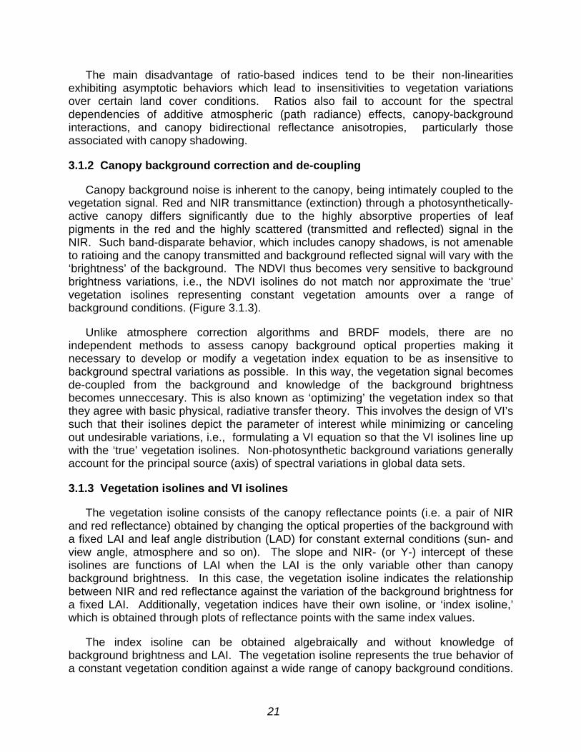
Figure 3.1.5: Derived vegetation isolines and the SAIL simulation data. The numbers inthe legend denote the LAI. 'iso' means the vegetation isoline. ..............................26

Figure 3.1.6: NDVI vs. LAI for the soil reflectance (red) of 0.05, 0.2, and 0.35. Themarks are the SAIL model and the lines are the vegetation isolines. .....................29

Figure 3.1.7: SAVI vs. LAI for the soil reflectance (red) of 0.05, 0.2, and 0.35. Themarks are the SAIL model and the lines are the vegetation isolines. .....................30

Figure 3.1.8: VI vs. LAI for different visibility with a constant soil brightness...................31

Figure 3.1.9: Landsat color composite and NDVI and EVI over a vegetated area with asmoke plume...........................................................................................................33

Figure 3.2.1: False color image (top) of the red, NIR and green SeaWiFS reflectancebands for one day worth of orbits. The incomplete coverage is due to the tilt-maneuvers above the equator and the swath width. White colors are clouds andsnow/ice patches. The second image (bottom) is a composition of 16consecutive days of SeaWiFS data, obtained by a MODIS like compositealgorithm. ................................................................................................................35

Figure 3.2.2: View and solar angular variations for several SeaWiFS orbits of one day.The right image is the color composite of red, NIR and green reflectance bands. .36

Figure 3.2.3: Illustration of MODIS data acquisition on the EOS-AM platform (not toscale). The bidirectional reflectance distribution function (BRDF) changes withview and sun geometry. Notice the shadow caused by clouds and canopy.MODIS pixel dimensions, cross-track and along-track, change with scan angles:0° - 250 x 250 m; 15° - 270 x 260 m; 30° - 350 x 285 m; 45° - 610 x 380 m(computed for the fine resolution red and NIR detectors; 250 m at nadir on theground). ..................................................................................................................38

vi

Figure 3.2.4: Flow diagram showing the relationship of relevant MODIS Land andAtmosphere Products (Level 1-L1; Level 2 - L2; Gridded L2-L2G; Level 3 - L3)that are required to generate the gridded, composited vegetation indices. ............43

Figure 3.2.5: Diagram showing the sequence of MODIS processing steps forcompositing of MODIS VI products at 250m and 1km spatial and 16 daystemporal resolution. ................................................................................................46

Figure 3.2.6: Diagram showing the sequence of MODIS processing steps for thecompositing of monthly MODIS VI products at 1km and 25km spatial resolution. ..47

Figure 3.2.7: Schematic overview of all the input files needed to produce the MOD13VI products and their associated science data sets................................................48

Figure 3.2.8: Continental NDVI profiles for the MODIS composite algorithm; AVHRR(8km).......................................................................................................................50

Figure 3.2.9: Example of temporal profiles of a) NDVI , b) red and NIR reflectancevalues, and c) sun and view zenith angles, for one pixel in a broadleaf deciduous(Lat. 22.92 °N, Long. 75.98°E) forest (vegetation classification based onKuchler’s (1995) world natural vegetation map) for the MODIS and the MVCcomposite approaches using AVHRR data. For each composite period theMODIS composite method is indicated with a number: 1- BRDF; 2 - CV-MVC; 3 -MVC........................................................................................................................51

Figure 3.2.10: Example of temporal profiles of NDVI, red and NIR reflectance valuesfor one desert vegetation pixel (Lat. 22.0°N, Long. 27.15°E) (vegetationclassification based on Kuchler’s (1995) world natural vegetation map) for the a)MVC and b) MODIS composite approaches using AVHRR data. For eachcomposite period the MODIS composite method is indicated with a number: 1-BRDF; 2 - CV-MVC. The sun zenith angle and view zenith angle are also shownfor each composite period. The negative and positive view angles are indicatedfor the respective backscatter and forward scatter view direction. The view zenithangle for the MODIS-BRDF corrected data is 0°. ...................................................52

Figure 3.2.11: Global NDVI image (pseudo color) using the MODIS VI compositealgorithm (BRDF/ CV-MVC/ MVC approach). .........................................................54

Figure 3.2.12: Color coded quality assurance flags for a Global NDVI composite usingthe MODIS approach (BRDF/CV-MVC/MVC); MVC (pr) the cloud mask indicatedthe pixels to be probably cloudy; MVC (cl)=cloudy pixels; land surfaces withoutdata were indicated with a dark color gray..............................................................54

Figure 3.2.13: Global view angle distribution (including all continents) for a 16-daycomposite period (August 13-August 28, 1989) for the MODIS (BRDF/CV-MVC)and CV-MVC and MVC algorithms .........................................................................55

vii

Figure 3.2.14: Global EVI (a) and NDVI (b) image (pseudo color) using the MODIS VIcomposite algorithm (BRDF/ CV-MVC/ MVC approach). (c) Color coded qualityassurance flags for a Global NDVI composite (very similar for EVI) using theMODIS approach (BRDF/CV-MVC/MVC) ...............................................................57-58

Figure 3.2.15: SEAWIFS color composite, NDVI, EVI and view angle distribution forSouth America. .......................................................................................................59

Figure 3.4.1: Vegetation index scientific algorithm operation flow....................................67

Figure 3.4.2: Vegetation Index algorithms major components .........................................69

Figure 3.4.3: Display of the Integerized sinusoidal projection as it will be tiled andgridded for the MODIS level 3 products. The horizontal tile ID’s (range0,35) andvertical tile ID's (range 0,17) are indicated in the border of the image. The tileswith land areas (green) and ocean (light blue) will be processed. Dark blueocean tiles will not be processed. White tiles are not covering any land or ocean .70

Figure 3.5.1: Mounted setup of the MQUALS radiometric package. ...............................81

Figure 3.5.2: Diagram of Exotech and camera airborne data acquisitions in relation to aMODIS pixel for 150 m AGL and 15 o field-of-view Exotech. ..................................82

Figure 3.5.3: Diagram of the traceability of field validation measurements to the MODISinstrument. ..............................................................................................................85

Figure 3.7.1: “End-to-end” analysis approaches of the VI error/uncertainties. Potentialsources of errors and uncertainties considered in each upstream processing stepare also listed..........................................................................................................90

Figure 3.7.2: Uncertainties of the a) NDVI, b) SAVI, c) ARVI, and d) EVI due to a 2%reflectance calibration uncertainty, ucal(VI), propagated through a turbidatmosphere (continental aerosols with a 10 km visibility). The band calibrationerrors were treated as uncorrelated. The figure includes ucal(VI) for dark(Cloverspring) and bright (Superstition) backgrounds.............................................92

Figure A1: Procedure to obtain vegetation isoline parameters.........................................110

viii

List of Tables

Table 1: MODIS sensor characteristics in support of the vegetation index algorithmproducts. .................................................................................................................15

Table 2: MODIS and SeaWiFS spectral bandwidths........................................................56

Table 3: The maximum and minimum mean solar zenith angles for land and thedifferent continents based on the AVHRR composited data. As expected, theapproximate Day of Year (DOY) the minimum and maximum sun angles occur,are during spring and fall. .......................................................................................60

Table 4: Storage loads of MODIS 13 I/O products ...........................................................72

Table 5: Summary of pre-launch validation activities .......................................................77

Table 6. Spectral characteristics of MQUALS components. .............................................81

Table 7: 1999 MQUALS deployments ..............................................................................85

Table 8: Predicted Reflectance Calibration Uncertainties (%) Requirements for DesiredLevels of VI Uncertainty..........................................................................................92

Table 9: Expected VI Error due to the Spectral Band Shift and Band-to-bandCoregistration Error (in VI unit) ...............................................................................93

1

1 Introduction

One of the primary interests of the Earth Observing System (EOS) program is tostudy the role of terrestrial vegetation in large-scale global processes with the goal ofunderstanding how the Earth functions as a system. This requires an understanding ofthe global distribution of vegetation types as well as their biophysical and structuralproperties and spatial/temporal variations. Remote sensing observations offer theopportunity to monitor, quantify, and investigate large scale changes in vegetation inresponse to human actions and climate. Vegetation influences the energy balance,climate, hydrologic, and biogeochemical cycles and can serve as a sensitive indicator ofclimatic and anthropogenic influences on the environment.

The MODIS vegetation indices (VIs) will provide consistent, spatial and temporalcomparisons of global vegetation conditions that will be used to monitor the Earth'sterrestrial photosynthetic vegetation activity for phenologic, change detection, andbiophysical derivation of radiometric and structural vegetation parameters. The MODISvegetation index (VI) products will play a major role in several EOS studies as well asbe an integral part in the production of many global and regional biospheric models andbiogeochemical cycles. Currently, satellite-derived vegetation indices are beingintegrated in interactive biosphere models as part of global climate modelling (Sellers etal. 1994; Raich and Schlesinger, 1992; Fung et al., 1987; Tans et al., 1990) andproduction efficiency models (Prince et al., 1994; Prince, 1991). They are also used fora wide variety of land applications, including natural resource management, agriculture,the Global Health and Human Monitoring Program (NASA, 1988), and operationalFamine Early Warning Systems (Prince and Justice, 1991; Hutchinson, 1991). Thislatter example is one of the few examples where derived satellite data are currentlybeing used to drive policy decisions.

1.1 Identification of Algorithm

MODIS product #13, Gridded Vegetation Indices (Level 3)

The level 3 gridded vegetation indices are standard products designed to be fullyoperational at launch. The level 3, spatial and temporal gridded vegetation indexproducts are composites of daily bidirectional reflectances. The gridded VIs are 16- and30 day spatial and temporal, re-sampled products designed to provide cloud-free,atmospherically corrected, and nadir-adjusted vegetation maps at nominal resolutionsof 250 m, 1 km, and 0.25°. The latter is also known as the climate modeling grid (CMG).

Two vegetation index (VI) algorithms are to be produced globally for land, at launch.One is the standard normalized difference vegetation index (NDVI), which is referred toas the “continuity index” to the existing NOAA-AVHRR derived NDVI. At the time oflaunch, there will be nearly a 20-year NDVI global data set (1981 - 1999) from theNOAA- AVHRR series, which could be extended by MODIS data to provide a long termdata record for use in operational monitoring studies. The other is an ‘enhanced’vegetation index with improved sensitivity to differences in vegetation from sparse to

2

dense vegetation conditions. The two VIs compliment each other in global vegetationstudies and improve upon the extraction of canopy biophysical parameters.

• Normalized Difference Vegetation Index (NDVI), Parameter No. 2749a

• Enhanced Vegetation Index (EVI), Parameter No. 4334a.

The compositing algorithm utilizes the bidirectional reflectance distribution functionof each pixel to normalize the reflectances to a nadir view and standard solar angulargeometry. The 16 day VI composites will be archived at 250 m resolution and willinclude the selected, nadir-adjusted VI value, the nadir-adjusted red and NIR surfacereflectances, median solar zenith, relative azimuth, and quality control parameters.

• 250 m NDVI (16 day)

• 1 km NDVI and EVI (16 day and monthly)

• 25 km NDVI and EVI (16 day and monthly)

The 250 m MODIS VI product will consist of only the NDVI, since the EVI utilizes the500 m blue channel and only the red and NIR bands are at 250 m resolution. Thecomposited surface reflectance data from each pixel will be used to compute both theNDVI and the EVI gridded products.

1.2 Key Science Applications of the Vegetation Index

Vegetation indices have a long history of use throughout a wide range of disciplines.Some examples are listed below:

• Inter- and intra-annual global vegetation monitoring on a periodic basis;

• Global biogeochemical, climate, and hydrologic modeling;

• Net primary production and carbon balance;

• Anthropogenic and climate change detection;

• Agricultural activities (plant stress, harvest yields, precision agriculture…);

• Famine early warning systems;

• Drought studies

• Landscape disturbances (volcanic, fire scars, etc..);

• Land cover and land cover change products;

• Biophysical estimates of vegetation parameters (%cover, fAPAR, LAI) ;

• Public health issues (rift valley fever, mosquito producing rice fields…).

3

2 Overview and Background Information

2.1 Experimental Objective

The overall objective is to design an empirical or semi-empirical robust vegetationmeasure applicable over all terrestrial biomes of the earth. Vegetation indices (VI’s) aredimensionless, radiometric measures of vegetation exploiting the unique spectralsignatures and behavior of canopy elements, particularly in the red and NIR portions ofthe spectrum. VI's not only map the presence of vegetation on a pixel basis, butprovides measures of the amount or condition of vegetation within a pixel. The basicpremise is to extract the vegetation signal portion from the surface. The stronger thesignal, the more vegetation is present for any given land cover type. Their principaladvantage is their simplicity. They require no assumptions, nor additional ancillaryinformation other than the measurements themselves. The goal becomes, how toeffectively combine these bands in order to extract and quantify the ‘green’ vegetationsignal across a global range of vegetation conditions while minimizing canopyinfluences associated with intimate mixing by non-vegetation related signals.

The vegetation index compositing objective is to combine multiple images into asingle, gridded, and cloud-free VI map, taking into account the variable atmosphereconditions, residual clouds, and a wide range of sensor view and sun angle conditions.The task is to design an algorithm that is able to depict spatial variations in vegetationacross a range of scales as well as depict temporal variations for phenologic studies(intra-annual) and change detection studies (inter-annual).

Specific tasks and experimental objectives include:

• develop precise, empirical measures of vegetation, depicting both spatial andtemporal variations in vegetation composition, condition, and photosyntheticactivity.

• continuity with current, global NOAA-AVHRR series, NDVI data fields.

• improved measures of vegetation utilizing new, improved variants of the NDVI forenhanced vegetation sensitivity and more accurate quantitative analysis.

• develop near-linear measures of vegetation parameters in order to maintainsensitivity over as wide a range of vegetation conditions as possible and tofacilitate scaling and extrapolations across regional and global resolutions.

• provide estimates of biophysical parameters, comparable for insertion into globalbiome and climate models.

• maximize global and temporal land coverage at the finest spatial and temporalresolutions possible within the constraints of the instrument characteristics andland surface properties.

• minimize the effects of residual clouds, cloud shadow, and atmosphericaerosols.

4

• standardize variable sensor view and sun angle (BRDF effects) of the cloud-freepixels to a nadir view angle and nominal sun angle.

• ensure the quality and consistency of the composited data.

2.2 Historical Perspective

2.2.1 Vegetation indices

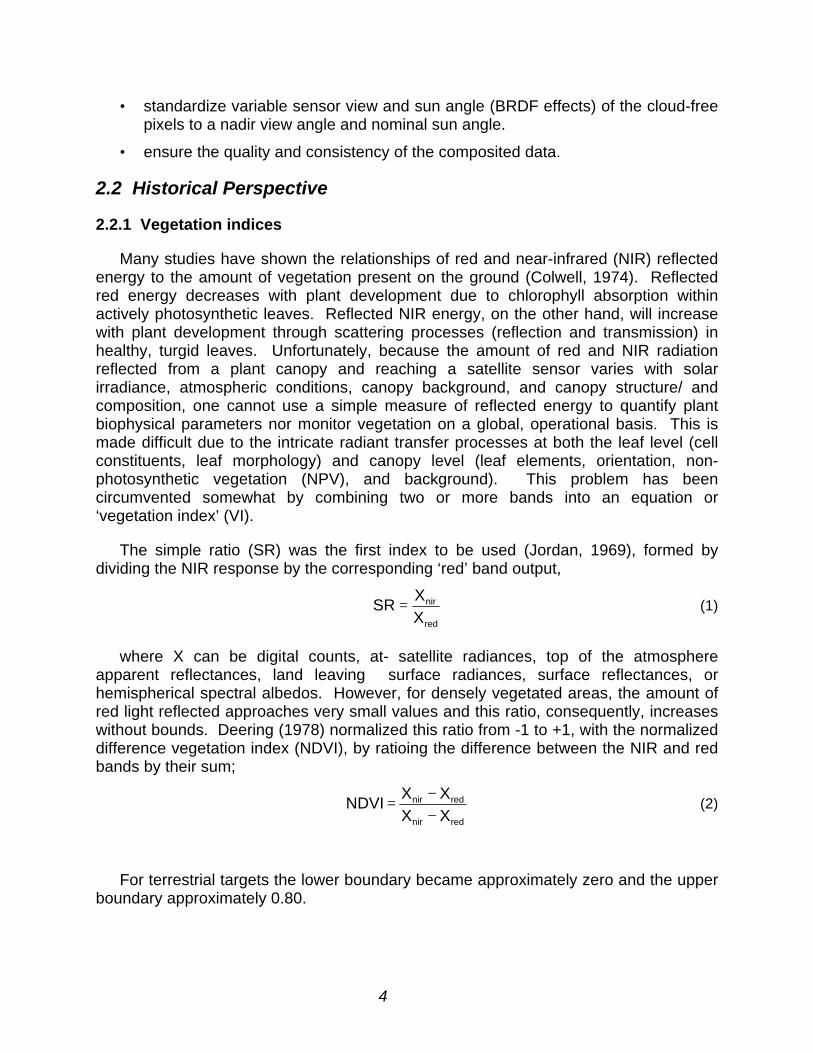
Many studies have shown the relationships of red and near-infrared (NIR) reflectedenergy to the amount of vegetation present on the ground (Colwell, 1974). Reflectedred energy decreases with plant development due to chlorophyll absorption withinactively photosynthetic leaves. Reflected NIR energy, on the other hand, will increasewith plant development through scattering processes (reflection and transmission) inhealthy, turgid leaves. Unfortunately, because the amount of red and NIR radiationreflected from a plant canopy and reaching a satellite sensor varies with solarirradiance, atmospheric conditions, canopy background, and canopy structure/ andcomposition, one cannot use a simple measure of reflected energy to quantify plantbiophysical parameters nor monitor vegetation on a global, operational basis. This ismade difficult due to the intricate radiant transfer processes at both the leaf level (cellconstituents, leaf morphology) and canopy level (leaf elements, orientation, non-photosynthetic vegetation (NPV), and background). This problem has beencircumvented somewhat by combining two or more bands into an equation or‘vegetation index’ (VI).

The simple ratio (SR) was the first index to be used (Jordan, 1969), formed bydividing the NIR response by the corresponding ‘red’ band output,

red

nir

XX

SR = (1)

where X can be digital counts, at- satellite radiances, top of the atmosphereapparent reflectances, land leaving surface radiances, surface reflectances, orhemispherical spectral albedos. However, for densely vegetated areas, the amount ofred light reflected approaches very small values and this ratio, consequently, increaseswithout bounds. Deering (1978) normalized this ratio from -1 to +1, with the normalizeddifference vegetation index (NDVI), by ratioing the difference between the NIR and redbands by their sum;

rednir

rednir

XXXX

NDVI−−

= (2)

For terrestrial targets the lower boundary became approximately zero and the upperboundary approximately 0.80.

5

Global-based operational applications of the NDVI have utilized digital counts, at-sensor radiances, ‘normalized’ reflectances (top of the atmosphere), and more recently,partially atmospheric corrected (ozone absorption and molecular scattering)reflectances. Thus, the NDVI has evolved with improvements in measurement inputs.Currently, a partial atmospheric correction for Rayleigh scattering and ozone absorptionis used operationally for the generation of the Advanced Very High ResolutionRadiometer; Agbu et al., 1994, (AVHRR) Pathfinder and the IGBP Global 1km NDVIdata sets (James and Kalluri 1994; Townshend et al. 1994). The NDVI is currently theonly operational, global-based vegetation index utilized. This is in part, due to its‘ratioing’ properties, which enable the NDVI to cancel out a large proportion of signalvariations attributed to calibration, noise, and changing irradiance conditions thataccompany changing sun angles, topography, clouds/shadow and atmosphericconditions.

As a vegetation monitoring tool, the NDVI is utilized to construct seasonal, temporalprofiles of vegetation activity enabling interannual comparisons of these profiles. Thetemporal profile of the NDVI has been shown to depict seasonal and phenologicactivity, length of the growing season, peak greenness, onset of greenness, and leafturnover or 'dry-down' period. Myneni et al. (1997) presented a 10 year NDVI datarecord of northern Boreal forests showing a warming trend whereby the length of thegrowing season had increased by nearly 2 weeks. They showed the usefulness of suchNDVI growing season plots for change detection and monitoring. Tucker (1985)similarly used NDVI seasonal profiles to show desert expansions and contractions inthe Sahara. The time integral of the NDVI over the growing season has beencorrelated with net primary production (NPP) (Running and Nemani, 1988; Prince,1991; Justice et al., 1985; Goward et al., 1991, Tucker and Sellers, 1986).

Many studies have shown the NDVI to be related to leaf area index (LAI), greenbiomass, percent green cover, and fraction of absorbed photosynthetically activeradiation (fAPAR) (Asrar et al., 1984; Baret and Guyot, 1991; Goward and Huemmrich,1992; Sellers, 1985; Sellers, 1986; Running and Nemani, 1988; Tucker et al., 1981;Curran, 1980). Relationships between fAPAR and NDVI have been shown to be nearlinear (Pinter, 1993; Begué, 1993; Wiegand et al., 1991; Daughtry et al., 1992), incontrast to the non-linearity experienced in LAI – NDVI relationships with saturationproblems at LAI values over 2. Other studies have shown the NDVI to be related tocarbon-fixation, canopy resistance, and potential evapotranspiration allowing its use asinput to models of biogeochemical cycles (Raich and Schlesinger, 1992; Fung et al.,1987; Sellers, 1985; Asrar et al., 1984; Running et al., 1989; Running, 1990; IGBP,1992).

2.2.2 Compositing

The construction of seasonal, temporal profiles requires a separate ‘compositing’algorithm in which several VI images, over a given time interval (7-days, 10-days, etc…)are merged to create a single cloud-free image VI map with minimal atmospheric andsun-surface-sensor angular effects (Holben, 1986). Moderate and coarse resolutionsatellite systems, such as MODIS, the AVHRR, SPOT4-VEGETATION (Systeme Pour

6

l’Observation de la Terre 4-VEGETATION; Archard et al., 1994), SeaWiFS (Sea-Viewing Wide Field-of-View Sensor; Hooker et al., 1994), and GLI (Global Imager;Nakajima et al., 1998) acquire global bi-directional radiance data of the Earth’s surfaceunder a wide variety of solar illumination angles, sensor view angles, atmospheres, andcloud conditions.

The current procedure for generation of composited, AVHRR-based, NDVI productsis the maximum value compositing (MVC) technique. This is accomplished byselecting, on a pixel by pixel basis, the input pixel with the highest NDVI value as outputto the composited product. The procedure generally includes cloud screening and dataquality checks (Goward et al., 1994; Eidenshink and Faundeer, 1994). Since residualcloud cover, not accounted for in the cloud masking procedure, and atmosphericsources of contamination both lower NDVI values, a maximum NDVI would select theleast cloud- and atmospheric-contaminated pixels. Furthermore, since the influence ofatmospheric contamination and residual cloud cover increases with optical path length,the maximum NDVI criterion also has a tendency to select the most near-nadir view andsmallest solar zenith angle pixels (least optical path lengths), thus standardizing to acertain degree the variable sun-surface-sensor observation geometries over acompositing cycle (Holben 1986; Cihlar et al. 1994a).

The MVC works nicely over near-Lambertian surfaces where the primary source ofpixel variations within a composite cycle is associated with atmosphere contaminationand path length, however, its major shortcoming is that the anisotropic, bi-directionalinfluences of the surface is not considered. The bidirectional spectral behavior ofnumerous, ‘global’ land cover types and terrestrial surface conditions have been widelydocumented and shown to be highly anisotropic due to canopy structure, shadowing,and background contributions (Kimes et al., 1985; Leeuwen et al., 1994; Vierling et al.,1997). Ratioing of the NIR and red spectral bands to compute vegetation indices doesnot remove surface anisotropy (Walter-Shea et al., 1997) due to the spectraldependence of the BRDF response (Gutman, 1991; Roujean et al., 1992). Theatmosphere counteracts and dampens the surface BRDF signal, mainly through theincreasing path lengths associated with off-nadir view angles and/or sun angles.

The maximum NDVI value selected is thus, related to both the bidirectionalproperties of the surface and the atmosphere, which renders the MVC-based selectionunpredictable. The MVC favors cloud free pixels, but does not necessarily pick the pixelclosest to nadir or with the least atmospheric contamination. Although the NDVI tendsto increase for atmospherically corrected data, it does not mean that the highest NDVIis an indication of the best atmospheric correction. Many studies have shown the MVCapproach to select off-nadir pixels with large, forward-scatter (more shaded) viewangles and large solar zenith angles, which are not always cloud-free or atmosphereclear (Goward et al., 1991; Moody and Strahler, 1994; Cihlar et al., 1994b, 1997). Thisdegrades the potential use of the VI for consistent and accurate comparisons of globalvegetation types.

The MVC method works best for data uncorrected for atmosphere (Cihlar et al.,1994a), although numerous inconsistencies result (Gutman, 1991; Goward et al., 1991,

7

1994; Cihlar et al., 1994b, 1997). The MVC approach becomes less appropriate withatmospherically-corrected data sets, since the anisotropic behavior of surfacereflectances and vegetation indices is stronger (Cihlar et al., 1994b). The influence ofsurface anisotropy and bidirectional reflectances on the VI composited products willbecome more pronounced in the EOS era as a result of improved atmospheric removalalgorithms, which will accentuate differences and cause surface BRDF-relatedanisotropies to become more prominent (Cihlar et al.,1994a). In many cases, the nadirview direction may produce the lowest VI value, particularly in atmospherically correcteddata.

There are other alternatives to simply choosing the highest NDVI value over acompositing cycle. One may integrate or average all cloud-free pixels over the period.Meyer et al. (1995) suggested that averaging the NDVI would be superior to the MVCapproach. The Best Index Slope Extraction (BISE; Viovy et al., 1992) method reducesnoise in NDVI time series by selecting against spurious high values through a slidingcompositing cycle. Use of the thermal channel has also been shown to be helpful.Knowledge of the ecological evolution of a land cover with respect to a VI temporalresponse might also be of use for the improvement of compositing techniques (Viovy etal.,1992; Qi et al., 1994; Moody and Strahler, 1994). This was not considered for theMODIS compositing algorithm due to the amount of knowledge required of thedynamics of land cover growth patterns, seasonality, and response to climate change(precipitation, temperature). Such an approach might be more applicable at regionalscales. Other VI compositing techniques are discussed by Cihlar et al. (1994b) and Qiand Kerr (1997).

2.2.3 VI optimization

The global operational use of a vegetation index requires that it not only becalculated in a uniform manner, but that the results be comparable over time andlocation. Although the NDVI has been shown useful in change detection, land surfacemonitoring, and in estimating many biophysical vegetation parameters, there is a historyof vegetation index research identifying limitations in the NDVI, which may impact uponits utility in global studies. These limitations form the basis of VI optimizationtechniques and are useful to understand before utilization of the VI product. Thelimitations can result from various external influences including:

• Calibration and instrument characteristics

• Clouds and cloud shadows

• Atmospheric effects due to variable aerosols, water vapor, and residual clouds.

• Sun-target-sensor geometric configurations and the resulting interactions ofsurface and atmospheric anisotropies on the angular dependent signal.

In addition to these external influences, there are influences inherent to vegetatedcanopies which restrict the use and/or interpretation of vegetation indices. Theseinclude:

8

• Canopy background contamination in which the background reflected signalintimately mixes with the vegetation signal and influences the resulting VI value.Canopy background signals vary with soils, litter covers, snow, and surfacewetness.

• Saturation problems whereby VI values remain invariant to changes in theamount, type, and condition of vegetation, normally associated with a saturatedchlorophyll signal in densely vegetated canopies.

Furthermore, if one were to extend VI capabilities to the derivation of biophysicalvegetation parameters, then one must take into account the following:

• Canopy structural effects associated with leaf angle distributions, clumping andnon-photosynthetically-active components (woody, senesced, and dead plantmaterials). Thus for a given LAI, %cover, and/ or biomass, the NDVI may varywith changes in the structure and orientation of the canopy. The ‘strength’ of thevegetation signal is simultaneously dependent upon several 'physical' measuresof vegetation amount, including leaf area index, %green cover, and wet or drygreen biomass.

• Non-linearity in VI relationships with fAPAR and/ or LAI.

2.2.4 Calibration and instrument characteristics

2.2.5 Atmospheric effects

The atmosphere degrades the NDVI value by reducing the contrast between the redand NIR reflected signals. The red signal normally increases as a result of scattered,upwelling path radiance contributions from the atmosphere, while the NIR signal tendsto decrease as a result of atmospheric attenuation associated with scattering and watervapor absorption. The net result is a drop in the NDVI signal and an underestimation ofthe amount of vegetation at the surface. The degradation in NDVI signal is dependenton the aerosol content of the atmosphere, with the turbid atmospheres resulting in thelowest NDVI signals. The impact of atmospheric effects on NDVI values is mostserious with aerosol scattering (0.04 - 0.20 unit decreases), followed by water vapor(0.04 - 0.08), and Rayleigh scattering (0.02 - 0.04) (Goward et al. 1991; Teillet, 1989).

The atmosphere problem may be corrected through direct and indirect means(Kaufman and Tanre, 1996). Atmospheric effects on the MODIS VI’s will becomeminimal as a result of the atmospheric correction algorithms being implemented(MODIS-09) prior to VI computation. However, some residual aerosol contaminationwill be expected in the NDVI product, due to the coarse resolution of the aerosolproduct (~20 km resolution) (Vermote et al., 1994) compared to the 250m NDVIproduct. Thus, spatial variations in smoke, gaseous and particulate pollutants, and lightcirrus clouds, may be present at the finer spatial resolutions. The accuracy ofatmospheric correction will also vary with the availability of ‘dark-objects’, which areneeded for the best corrections.

9

Kaufman and Tanré (1992) developed the atmospherically resistant vegetationindex (ARVI) as an example of an indirect approach to atmosphere correction, utilizingthe difference of the blue and red bands as an indicator of atmospheric noise. TheARVI accounts for atmosphere aerosol scattering and requires atmospheric correctionof molecular scattering and ozone absorption prior to its use. Myneni and Asrar (1993),in a sensitivity study with simulated data, found the ARVI to reduce atmospheric effectsand to mimic ground-based NDVI data. Pinty and Verstraete (1992) have proposed anAVHRR-specific, global environment monitoring index (GEMI), which minimizesatmospheric effects specific to AVHRR data sets. We propose to use the atmosphereresistance concept (blue/ red) in the enhanced VI (EVI) to aid with highly variableaerosol conditions, such as smoke from biomass burning.

2.2.6 Angular considerations

The NDVI has been shown to be affected by variations in bidirectional reflectancesresulting from differences in sun-target-sensor geometries. MODIS viewing angles willvary ±55° cross-track accompanied by solar illumination angle differences of up to 20°from edge to edge of the MODIS swath. In addition sun angles will vary with latitudeand time of the year. The strong anisotropic properties from vegetation canopiesseriously affect vegetation indices, an effect that will become more pronounced withMODIS data in which atmosphere correction will further enhance surface-basedanisotropies, which vary with land cover type, relative amounts of characteristicvegetation and soil components, and sun-earth-sensor geometry. The resultingdeviations must be considered in the derivation of the vegetation index products. Thisresulting variability in view and sun angles is important for the (seasonal andinterannual) intercomparison of vegetative covers on a global basis. Therefore, someknowledge of the bi-directional reflectance distribution function (BRDF) is needed forsuccessful utilization of directional reflectance data and vegetation indices, and thederivation of land cover-specific biophysical parameters (Cihlar et al., 1994a).

The influence of variable sun-target-sensor configurations on derived vegetationindices can be standardized in various manners, including: (1) standardize reflectancesto nadir view angle at a solar zenith angle representative of the observations; (2)standardize reflectances to nadir view angle and a temporally and globally constantsolar zenith angle; (3) adjust to a constant “off-nadir” view angle with a constant sunangle; or (4) use of spectral (bi-hemispherical) albedos. For the standard MODIS VIproducts, we propose to use the first method (Justice et al., 1998) and examine theother three approaches post-launch. There is considerable research and understandingof bidirectional reflectances with the development of physical, semi-empirical, andempirical BRDF models (Wanner et al., 1995). Preliminary analysis (Huete et al., 1996)also suggests that both the third and fourth approaches may enhance vegetationdetection only over a limited range of land cover conditions (Kimes et al., 1984; Privetteet al., 1996), and will result in overall decreased sensitivity from desert to forest, andpresent greater saturation problems in more densely vegetated canopies.

10

2.2.7 Canopy background contamination

In contrast to the previous sources of noise and uncertainty, this source ofuncertainty is best handled in the formulation of the VI equation itself, since canopybackground (soil, litter, snow, and water) effects on the VI are not readily corrected forprior to VI computation. Background effects are best removed within the VI equationitself because (1) they cannot be assessed independently as in atmosphere and BRDF;and (2) in validation, a ‘true’ VI value for a given canopy is needed, one that does notdepend upon the background optical properties.

Numerous ground-, air-, and satellite-based observations have shown the NDVI tobe overly sensitive to the brightness of the underlying canopy background (Elvidge andLyon, 1985; Huete et al., 1985; Heilman and Kress, 1987; Huete and Warrick, 1990; Qiet al., 1993a). Canopy backgrounds exhibit spatial and temporal reflectance variationsresulting from rain events, snowfall, litterfall, roughness, and the organic matter contentand mineralogy of the soil substrate material. In all of these studies there is asystematic increase in the NDVI value as the reflectance or ‘brightness’ of thebackground decreases. This change in NDVI with background brightness is alsoconfirmed with canopy radiative transfer models including the SAIL and two-streamapproximation models (Baret and Guyot, 1991; Baret at al., 1989; Myneni and Asrar,1993); Sellers, 1985; Choudhury, 1987). Goward and Huemmrich (1992) noted howdifficult it is to observe or quantify background effects in global scale imagery, althoughsnow background was deemed to be of particular concern, introducing errors in theestimation of fAPAR in excess of 50% relative to more typical canopy backgrounds (soiland litter), where errors were in excess of ±15%.

A common misconception is that canopy background considerations are onlyimportant in sparsely vegetated, arid and semi-arid areas, where spectral variations inbackground are the greatest. However, most studies and simulations show NDVIbackground sensitivity to be greatest at intermediate levels of vegetation, comparable tohumid and sub-humid land cover types, including open forest stands. Bausch (1993)and Huete et al. (1985) showed the influence of canopy background reflectance onNDVI values to be highest at LAI = 1 (~40% green cover) where the NDVI varied by0.30 units for background reflectances that varied from 0.06 to 0.33 in the red.Background influences start to disappear at LAI > 2, which is where ‘saturation’ begins.The range in background reflectances becomes greater when snow, wetlands, andirrigated rice paddy fields are included.

Several approaches have been proposed to minimize background influences onvegetation indices. Richardson and Wiegand (1977) introduced the perpendicularvegetation index (PVI) which utilized a ‘soil line’ concept for site specific backgroundcorrections. The soil line is a “baseline” value of zero vegetation over a wide‘brightness’ range of soil backgrounds, from which vegetation can be measured in NIR-red space, relative to the baseline. Clevers (1989) found the weighted differencevegetation index (WDVI) to greatly improve upon the estimation of LAI while minimizingbackground effects. Elvidge and Chen (1995) showed how narrower-band channels, asinput to vegetation indices, reduce background-related problems present in broad-band

11

vegetation indices. Similarly, Hall et al. (1990) and Demetriades-Shah et al. (1990)have discussed the value of narrow-band, derivative spectra for reducing backgroundeffects. Major et al. (1990) proposed a series of ratio-based vegetation indices, whicheffectively estimated the slope of the vegetation isoline derived with a simplereflectance model (Baret and Guyot, 1991).

Some studies have utilized knowledge of vegetation isoline equations, derived fromsimple reflectance models, to produce vegetation indices which minimize soilbackground effects (Huete 1988: Major et al. 1990). The soil-adjusted vegetation index(SAVI), proposed by Huete (1988), uses vegetation isoline equations derived byapproximating canopy reflectances by a first-order photon interaction model betweencanopy and soil layers (Huete 1987). This was further improved by Baret et al. (1989)yielding the transformed soil adjusted vegetation index (TSAVI) and by Qi et al. (1993b)with the modified SAVI (MSAVI).

Canopy background influences on vegetation indices are also atmosphere-sensitive,Huete and Liu (1994) found background influences on the NDVI to decrease greatlywith increases in atmospheric aerosol contents and that at a horizontal visibility of 5km(turbid atmosphere), background influences became nearly zero. This was alsoobserved with satellite imagery (Qi et al., 1993). Consequently, we anticipate canopybackground problems to become more pronounced in MODIS-NDVI imagery due to theimproved atmospheric correction algorithms being implemented. A feedback problemis evident whereby the improvement of one form of noise increases other forms ofnoise. Liu and Huete (1995) developed a feedback-based approach to correct for theinteractive canopy background and atmospheric influences, incorporating bothbackground adjustment and atmospheric resistance concepts. This enhanced, soil andatmosphere resistant vegetation index (EVI) was simplified to:

)CC(L

)(2EVI

blue2red1nir

rednir

ρ+ρ+ρ+ρ−ρ

⋅= (3)

where ρ is ‘apparent’ (top-of-the-atmosphere) or ‘surface’ directional reflectances, L is acanopy background adjustment term, and C1 and C2 weigh the use of the blue channelin aerosol correction of the red channel (Huete and Liu, 1996).

2.2.8 NDVI saturation considerations

There are several explanations for the NDVI saturation problem over denselyvegetated areas in which NDVI values no longer respond to variations in greenbiomass. The NDVI has been reported to be an insensitive measure of LAI at valuesexceeding 2 or 3. This is of concern since land use change detection, vegetationmonitoring, net primary production, and scaling studies cannot be carried out in anNDVI ‘saturated’ mode (Townshend et al., 1991). Land cover classification based onmultitemporal NDVI profiles would similarly be hampered. Gitelson et al. (1996)attributed this to the high sensitivity of the NDVI to the red (chlorophyll) absorptionband, which also saturates quickly. Maximum sensitivity to chlorophyll-a (Chl-a )pigment absorption is at 670nm. For Chl-a concentration beyond 3-5 µg/cm2 , the

12

inverse relationship of reflectance at 670nm vs. chlorophyll concentration ‘saturates’and is no longer sensitive despite a global range in chlorophyll concentrations from 0.3to 45 µg/cm2 (Vogelmann et al. 1994; Buschmann and Nagel 1993).

Gitelson et al. (1996) reported enhanced sensitivity could be achieved by replacingthe red channel with a green channel, which was found to remain sensitive tochlorophyll-a over a wider range of concentrations. They proposed a green NDVIequation which was five times more sensitive to Chl-a concentration. Yoder andWaring (1994) similarly have used a green NDVI for improved estimates ofphotosynthetic activity in Douglas-fir trees. The potential, however, for improvedvegetation analysis with narrower-band channels is also well demonstrated (Elvidgeand Chen 1995). This is of concern to the MODIS-NDVI equation because the MODISred channel is much narrower (620 - 670nm) and chlorophyll-sensitive than that of theAVHRR (580 - 680nm) and may thus saturate more quickly.

Although bandwidth may affect saturation, one must also consider the nature of theNDVI mathematical transform involving the red and NIR bands. The NDVI is a non-linear ‘stretch’ of the functionally equivalent, NIR/red ratio designed to confine its valuesfrom -1 to +1 (Deering, 1978). The stretch has the effect of enhancing low ratio valueswhile compressing higher ratio values. As ratio values increase from 5 to 10 and 15,the corresponding NDVI values shift from 0.67 to 0.82 (20% increase), and 0.87 (6%increase). A further increase in the NIR/red ratio to a value of 20 yields very littlechange in the NDVI (0.90). The non-linear stretch has the effect of enhancingvegetation index values under low biomass conditions while compressing the NDVIvalues at high biomass conditions. This results in very low sensitivity to spatial andtemporal variations in densely vegetated areas.

2.2.9 Canopy structural effects (biophysical interpretations):

Sellers (1985) calculated the variation of the NDVI with canopy greenness fractionsand demonstrated how the presence of dry and dead plant material severely alters therelationship between NDVI and LAI. He showed the NDVI to vary greatly with leafangle which alters the optical thickness of the canopy. He also showed that due to thenon-linear nature of the NDVI-LAI relationship, the contribution of the bare groundfraction to the NDVI is disproportionately strong when equal amounts of greenness(LAI) are distributed differently, such as in clumps. The same LAI in smaller coverfractions yielded the lowest NDVI. Clevers and Verhoef (1993) used the SAIL canopyand PROSPECT leaf models to show how the main variable that influences vegetationindices is the leaf inclination angle distribution. The more planophile a canopy thegreater the vegetation index value for a given LAI.

Because of the overwhelming influence of canopy structure on spectral reflectancesand vegetation indices, it is very difficult to derive biophysical plant parameters directlyfrom the VI. Many of the VI to biophysical parameter relationships involve site specific,regression plots which are subject to variability associated with canopy background,atmosphere, instrument calibration, sun angle, and view angle. It is necessary toaccomodate the effects of the different factors when interpreting VI values, especially if

13

we are to detect deviations in behavior indicative of directional or ‘global’ change(Wickland, 1989; Prince and Justice, 1991). A direct approach would be to utilize acanopy radiative transfer model to handle the radiative transfer processes within thestructure of the canopy. Alternatively, an indirect approach may be utilized whereby‘land cover type’ empirical parameters are used in the translation from NDVI to LAI,green cover, or fAPAR.

2.2.10 Vegetation indices, summary

The MODIS VI’s are envisioned as improvements over the current NOAA-AVHRRNDVI as a result of both improved instrument design and characterization and thesignificant amount of VI research conducted over the last decade. Many new indiceshave been proposed to further improve upon the ability of the NDVI to estimatebiophysical vegetation parameters (Prince et al., 1994). However, the robustness andglobal implementation of these indices have not been tested and one must be cautiousthat new problems are not created by removing the ‘ratioing’ properties of the NDVI.The ‘ratioing’ properties of the NDVI were extremely vital when the NOAA-AVHRRproduction of the NDVI first began, particularly with un-normalized, uncalibrated, anduncorrected for atmosphere data sets. Since the MODIS NDVI product will utilize well-calibrated and atmospherically corrected, surface reflectances, one needs to re-assessthe continued importance and benefits of ‘ratios’.

On one hand there is a need for continuity, while on the other hand improvements tomake the NDVI more quantitative are needed. In the next section of this algorithm,“Algorithm Description”, we describe the implementation of multiple indices and assesstheir capability in improving vegetation monitoring and change detection.

In summary, the criteria for and definition of a global vegetation index includes:

• the index should maximize sensitivity to plant biophysical parameters, preferablywith a linear response in order that some degree of sensitivity be available for awide range of vegetation conditions and to facilitate validation and calibration ofthe index,

• the index should normalize or model external effects such as sun angle, viewingangle, and atmosphere for consistent spatial and temporal comparisons,

• the index should normalize canopy background (brightness) variations forconsistent spatial and temporal comparisons,

• the index should be applicable to the generation of a global product, allowingprecise and consistent, spatial and temporal comparisons of vegetationconditions,

• the index should be coupled to key biophysical parameters such as LAI andfAPAR as part of the validation effort, performance, and quality control.

14

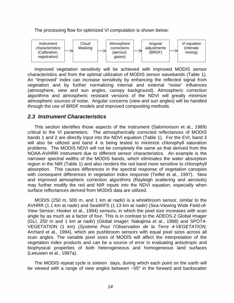
The processing flow for optimized VI computation is shown below:

Improved vegetation sensitivity will be achieved with improved MODIS sensorcharacteristics and from the optimal utilization of MODIS sensor wavebands (Table 1).An “improved” index can increase sensitivity by enhancing the reflected signal fromvegetation and by further normalizing internal and external “noise” influences(atmosphere, view and sun angles, canopy background). Atmospheric correctionalgorithms and atmospheric resistant versions of the NDVI will greatly minimizeatmospheric sources of noise. Angular concerns (view and sun angles) will be handledthrough the use of BRDF models and improved compositing methods.

2.3 Instrument Characteristics

This section identifies those aspects of the instrument (Salomonson et al., 1989)critical to the VI parameters. The atmospherically corrected reflectances of MODISbands 1 and 2 are directly input into the NDVI equation (Table 1). For the EVI, band 3will also be utilized and band 4 is being tested to minimize chlorophyll saturationproblems. The MODIS NDVI will not be completely the same as that derived from theNOAA-AVHRR instrument due to different sensor characteristics. An example is thenarrower spectral widths of the MODIS bands, which eliminates the water absorptionregion in the NIR (Table 1) and also renders the red band more sensitive to chlorophyllabsorption. This causes differences in the spectral response of vegetation canopieswith consequent differences in vegetation index response (Teillet et al., 1997). Newand improved atmospheric correction algorithms (Rayleigh scattering and aerosols)may further modify the red and NIR inputs into the NDVI equation, especially whensurface reflectances derived from MODIS data are utilized.

MODIS (250 m, 500 m, and 1 km at nadir) is a whiskbroom sensor, similar to theAVHRR (1.1 km at nadir) and SeaWiFS (1.13 km at nadir) (Sea-Viewing Wide Field-of-View Sensor; Hooker et al., 1994) sensors, in which the pixel size increases with scanangle by as much as a factor of four. This is in contrast to the ADEOS-2 Global Imager(GLI, 250 m and 1 km at nadir) (Global Imager; Nakajima et al., 1998) and SPOT4-VEGETATION (1 km) (Systeme Pour l’Observation de la Terre 4-VEGETATION;Archard et al., 1994), which are pushbroom sensors with equal pixel sizes across allscan angles. The variable pixel sizes of MODIS will affect the interpretation of thevegetation index products and can be a source of error in evaluating anisotropic andbiophysical properties of both heterogeneous and homogeneous land surfaces(Leeuwen et al., 1997a).

The MODIS repeat cycle is sixteen days, during which each point on the earth willbe viewed with a range of view angles between ~55° in the forward and backscatter

Instrumentcharacteristics(Calibration,registration)

CloudMasking

Atmospherecorrections(aerosol,gases)

Angularadjustments

(BRDF)

VI equation(intimatemixing)

15

direction. The scan angle is slightly lower than the view zenith angle due to thecurvature of the earth. Complete coverage of the earth may further be attained within ascan angle of 20° in an 8-day period. Since the repeat cycle is 16 days, it is suggestedto make the compositing period half of this time, thus 8 days. This number seemsappropriate since it gives a consistent distribution of view angles and a possibility tocover all latitudes within small viewing angles, providing the best spatial resolution (250m NDVI) and most accurate atmospheric correction.

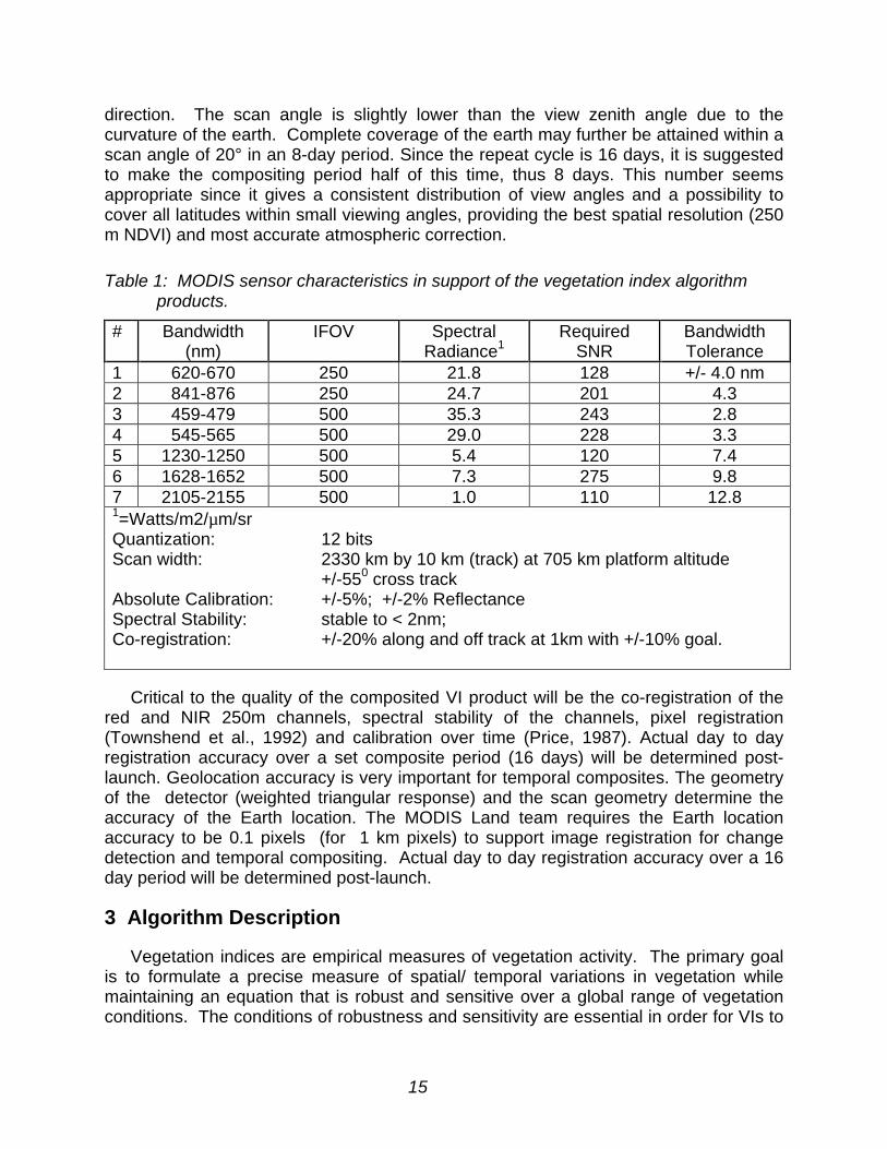
Table 1: MODIS sensor characteristics in support of the vegetation index algorithmproducts.

# Bandwidth(nm)

IFOV SpectralRadiance1

RequiredSNR

BandwidthTolerance

1 620-670 250 21.8 128 +/- 4.0 nm2 841-876 250 24.7 201 4.33 459-479 500 35.3 243 2.84 545-565 500 29.0 228 3.35 1230-1250 500 5.4 120 7.46 1628-1652 500 7.3 275 9.87 2105-2155 500 1.0 110 12.81=Watts/m2/µm/srQuantization: 12 bitsScan width: 2330 km by 10 km (track) at 705 km platform altitude

+/-550 cross trackAbsolute Calibration: +/-5%; +/-2% ReflectanceSpectral Stability: stable to < 2nm;Co-registration: +/-20% along and off track at 1km with +/-10% goal.

Critical to the quality of the composited VI product will be the co-registration of thered and NIR 250m channels, spectral stability of the channels, pixel registration(Townshend et al., 1992) and calibration over time (Price, 1987). Actual day to dayregistration accuracy over a set composite period (16 days) will be determined post-launch. Geolocation accuracy is very important for temporal composites. The geometryof the detector (weighted triangular response) and the scan geometry determine theaccuracy of the Earth location. The MODIS Land team requires the Earth locationaccuracy to be 0.1 pixels (for 1 km pixels) to support image registration for changedetection and temporal compositing. Actual day to day registration accuracy over a 16day period will be determined post-launch.

3 Algorithm Description

Vegetation indices are empirical measures of vegetation activity. The primary goalis to formulate a precise measure of spatial/ temporal variations in vegetation whilemaintaining an equation that is robust and sensitive over a global range of vegetationconditions. The conditions of robustness and sensitivity are essential in order for VIs to

16

be effective in intercomparisons of vegetation and extraction of biophysical parametersfrom arid regions to rainforest areas. The vegetation index equations presented hereutilize the red and NIR reflected signals to isolate and enhance the ‘green’,photosynthetically-active vegetation component of a given pixel. The red and NIRresponses are radiometrically calibrated, cloud-filtered, atmospherically corrected,spatially and temporally gridded, and adjusted for view angle influences to produce thelevel 3 vegetation index maps. The level 3 products are 16- and 30-day, cloud-freevegetation maps at 250 m, 1 km, and 0.25o spatial resolutions.

In discussing VI robustness and sensitivity to vegetation “variations”, it is useful toexpress such measures of performance in terms of various physical parameters of thevegetation such as LAI or %green cover. This also serves as a useful validation tool toensure that spatial and temporal variations depicted through the VI maps areassociated with ‘real’ changes in vegetation. In the following section the theory andphysical principles from which the VI products are derived are presented along with anassessment of their robustness as precise measures of vegetation activity. Thetheoretical basis of the NDVI is first presented followed by a theoretical basis for animproved vegetation index.

3.1 Theoretical Description of Vegetation Indices

The theoretical basis for ‘empirical-based’ vegetation indices is derived fromexamination of typical spectral reflectance signatures of leaves (Figure 3.1.1). Thereflected energy in the visible is very low as a result of high absorption byphotosynthetically active pigments with maximum sensitivity in the blue (470 nm) andred (670 nm) wavelengths. Nearly all of the near-infrared radiation is scattered(reflected and transmitted) with very little absorption, in a manner dependent upon thestructural properties of a canopy (LAI, leaf angle distribution, leaf morphology). As aresult, the contrast between red and near-infrared responses is a sensitive measure ofvegetation amount, with maximum red - NIR differences occurring over a full canopyand minimal contrast over targets with little or no vegetation (Figure 3.1.1). For low andmedium amounts of vegetation, the contrast is a result of both red and NIR changes,while at higher amounts of vegetation, only the NIR contributes to increasing contrastsas the red band becomes saturated due to chlorophyll absorption.

17

Figure 3.1.1: Spectral reflectance signature of a photosynthetically active leaf with asoil signature to show contrast (Tucker and Seller, 1986).

The red-NIR contrast can be quantified through the use of ratios (NIR/red),differences (NIR-red), weighted differences (NIR-k*red), linear band combinations (x1 *red + x2 * NIR), or hybrid approaches of the above. Vegetation indexes are measuresof this contrast and thus are integrative functions of canopy structural (%cover, LAI,LAD) and physiological (pigments, photosynthesis) parameters.

The contrast between red and NIR canopy reflectances for a variety of canopy typesand canopy backgrounds may also be depicted in graphical form, using the red andnear-infrared reflectances as axes. In such a plot, a triangular, cloud of points isobserved with well-defined boundaries, whether the data plotted are temporally variablereflectances of agricultural crops over the growing season (Figure 3.1.2a) or spatiallyvariable reflectances of different land covers from desert to forests (Figure 3.1.2b).

18

Figure 3.1.2a: Cloud of reflectance points in NIR-red waveband space for agricultural

crops observed throughout the growing season.

Figure 3.1.2b: Cloud of reflectance points in NIR-red reflectance space from Landsat

TM for a wide range of land surface cover types.

In both cases there is a lower ‘baseline’ of pixels close to the 1:1 line, representingthe lower boundary condition of vegetation. This baseline boundary condition can befurther extended to include water targets (dark), snow backgrounds (bright), soils withvariable mineralogies and litter and detrital material at variable stages of decomposition(bright to dark) or incorporation into the dark soil humus pool. The basic premise of thelower baseline is that only non-photosynthetic targets with low contrast in the red andNIR will occupy this area. The third apex represents dense vegetation which is at or

0 0.1 0.2 0.3 0.4 0.50

0.1

0.2

0.3

0.4

0.5

0.6

0.7

RED REFLECTANCE

NIRCORN

COTTON

SOIL

ALFALFA

WHEAT

NDVI=0

NDVI=0.80

NDVI=0.60NDVI=0.40

NDVI=0.20

0 0.05 0.1 0.15 0.2 0.25 0.30

0.1

0.2

0.3

0.4

0.5

R ED REFLECTA NC E

W ater

Arid

Se mi-ar id

Grass

D eciduo us forests

Conifer forest

19

close to the lowest red values (chlorophyll-absorption) and highest NIR values. Note,the lower baseline involves non-photosynthetic canopy backgrounds and would notinclude a separate understory canopy, i.e., multiple canopy layers are all treated asoverlying canopy and not background.

Pixels with increasing amounts of green vegetation shift away from the lowerbaseline toward the apex of maximum NIR and low red reflectance in a mannerdependent upon the optical/ structural properties of the vegetation canopy and theoptical properties of the canopy background (soil, snow, water, understory, etc.) (Figure3.1.2). The greater the amount of ‘green’ vegetation present in a pixel, the greater willbe the red-NIR contrast, and thus the shift away from the lower baseline. In Figure3.1.2b, desert regions fall near the lower zero ‘baseline’, followed by semi-arid andgrassland pixels. Closed forest canopies and open forests with green understoriesoccupy the extreme left-hand portion, varying very little in the red (‘saturation’) withlarger variations along the NIR axis (Figure 3.1.2), in accordance with expected opticalbehavior. The pixels inside the triangular cloud structure are generally ‘mixed’ pixels,with multiple responses from the vegetation and background components. Over 70% ofthe Earth’s terrestrial surface is classified as “open canopies” with mixed backgroundand vegetation signals (Graetz, 1990). The role of vegetation indices is to model thebehavior and boundary conditions of the cloud of terrestrial-based pixels in NIR-redspace and their associated variations in time and space.

Within the cloud of spectra we can identify pairs of red and NIR reflectances whichrepresent equal amounts of a particular vegetation parameter. This may be describedby the term "vegetation isoline" and may be derived via canopy radiative transfermodels and/or observational data sets. Vegetation Index isolines, on the other hand,represent all combinations of red and NIR reflectance responses resulting in the sameVI value. These are the model parameters which dissect the pixel data structure intovarious levels of vegetation amounts. They create the “gray levels” of the vegetationindex from low to high. The concept of isolines essentially connect radiative transfertheory with vegetation indices and provide a basis for decoupling atmosphere andbackground signals from the vegetation signal.

3.1.1 Theoretical basis of the NDVI

The NDVI is a ‘normalized’ transform of the NIR to red reflectance ratio, ρnir/ρred ,designed to standardize VI values to between –1 and +1;

+ρ

ρ

−ρ

ρ

=1)(

1)(NDVI

red

nir

red

nir

(4)

It is functionally equivalent to the NIR to red ratio and is more commonly expressed as:

[ ][ ]rednir

rednir

XX

XXNDVI

+−

= (5)

20

As a ratio, the NDVI has the advantage of minimizing certain types of band-correlated noise (positively-correlated) and influences attributed to variations indirect/diffuse irradiance, clouds and cloud shadows, sun and view angles, topography,and atmospheric attenuation. Ratioing can also reduce, to a certain extent, calibrationand instrument-related errors. The NDVI, as a ratio, can be computed from raw digitalcounts, top-of-the-atmosphere radiances, apparent reflectances (normalizedradiances), and partially or total atmospheric corrections. Although the units cancel out,the NDVI values themselves change so one must be consistent in how the NDVI isderived (Jackson and Huete, 1991). The extent to which ratioing can reduce noise isdependent upon the correlation of noise between red and NIR responses and thedegree to which the surface exhibits Lambertian behavior.

Ratios create simple, red-NIR space, vegetation index isolines (Figure 3.1.3) ofincreasing slopes diverging out from the origin, i.e., slopes increase with vegetationamount and intercepts are independent of vegetation amount with a constant value ofzero.

The NDVI efficiently shows increasing values from the baseline region to the ‘green’apex. Furthermore, the large range in background brightness values, with little or novegetation present, fall close to the 1:1 line showing that the NDVI is able to ratio out asignificant portion of these spectral variations with NDVI values constrained to valuesslightly above ‘zero’. The robustness of the NDVI is well established. As long as non-vegetation sources of spectral variation cause pixels to shift toward or away the origin, itis following an NDVI isoline or equal NDVI value. The NDVI is the only VI currentlyadapted to global processing and it is used extensively in global, regional, and localmonitoring studies. It has also been used on a wide array of sensors and platformsfrom Landsat MSS and TM, to the NOAA-AVHRR series, SPOT, SeaWiFS, AVIRIS,and ground-based radiometers.

In the following sections, we analyze in detail the limitations of the NDVI both for thepurpose of assessing product performance as well as to explore potential methods forimprovement while maintaining a robust and operational algorithm. Up to now theburden of noise removal in satellite data is placed on the NDVI equation itself and thusthe NDVI has the task of minimizing noise and simultaneously enhancing vegetationsignals. The remotely-sensed spectral signatures, however, vary with both external andinternal factors such as sensor calibration, atmosphere, sun- and view angles, andcanopy background. Because of these influences, VIs also show variations whichresult in inaccuracies in estimating vegetation biophysical parameters. Asadvancements are made in minimizing many of the external influences, such as sensorcalibration, noise removal, atmosphere correction, and BRDF modeling, other non-ratioing approaches, including canopy models, may be used to better depict vegetationspatial and temporal variations. For example, in contrast to the heritage AVHRR-NDVIproduct, the MODIS NDVI algorithm will utilize complete, atmospherically corrected,surface reflectance inputs. The instrument itself will be well calibrated and bandpassesare narrower, avoiding atmosphere contaminants such as water vapor.

21

The main disadvantage of ratio-based indices tend to be their non-linearitiesexhibiting asymptotic behaviors which lead to insensitivities to vegetation variationsover certain land cover conditions. Ratios also fail to account for the spectraldependencies of additive atmospheric (path radiance) effects, canopy-backgroundinteractions, and canopy bidirectional reflectance anisotropies, particularly thoseassociated with canopy shadowing.

3.1.2 Canopy background correction and de-coupling

Canopy background noise is inherent to the canopy, being intimately coupled to thevegetation signal. Red and NIR transmittance (extinction) through a photosynthetically-active canopy differs significantly due to the highly absorptive properties of leafpigments in the red and the highly scattered (transmitted and reflected) signal in theNIR. Such band-disparate behavior, which includes canopy shadows, is not amenableto ratioing and the canopy transmitted and background reflected signal will vary with the‘brightness’ of the background. The NDVI thus becomes very sensitive to backgroundbrightness variations, i.e., the NDVI isolines do not match nor approximate the ‘true’vegetation isolines representing constant vegetation amounts over a range ofbackground conditions. (Figure 3.1.3).

Unlike atmosphere correction algorithms and BRDF models, there are noindependent methods to assess canopy background optical properties making itnecessary to develop or modify a vegetation index equation to be as insensitive tobackground spectral variations as possible. In this way, the vegetation signal becomesde-coupled from the background and knowledge of the background brightnessbecomes unneccesary. This is also known as ‘optimizing’ the vegetation index so thatthey agree with basic physical, radiative transfer theory. This involves the design of VI’ssuch that their isolines depict the parameter of interest while minimizing or cancelingout undesirable variations, i.e., formulating a VI equation so that the VI isolines line upwith the ‘true’ vegetation isolines. Non-photosynthetic background variations generallyaccount for the principal source (axis) of spectral variations in global data sets.

3.1.3 Vegetation isolines and VI isolines

The vegetation isoline consists of the canopy reflectance points (i.e. a pair of NIRand red reflectance) obtained by changing the optical properties of the background witha fixed LAI and leaf angle distribution (LAD) for constant external conditions (sun- andview angle, atmosphere and so on). The slope and NIR- (or Y-) intercept of theseisolines are functions of LAI when the LAI is the only variable other than canopybackground brightness. In this case, the vegetation isoline indicates the relationshipbetween NIR and red reflectance against the variation of the background brightness fora fixed LAI. Additionally, vegetation indices have their own isoline, or ‘index isoline,’which is obtained through plots of reflectance points with the same index values.

The index isoline can be obtained algebraically and without knowledge ofbackground brightness and LAI. The vegetation isoline represents the true behavior ofa constant vegetation condition against a wide range of canopy background conditions.

22

These two types of isolines are typically different and usually do not coincide with eachother (Baret and Guyot, 1991; Huete, 1988; Major et al., 1990; Qi et al., 1994) (e.g.,NDVI in Figure 3.1.3), causing the NDVI value to vary with variations in the backgroundbrightness. In order to have a VI invariant to background brightness variation, the indexisolines must be coincident with the 'true' vegetation isolines. The knowledge of thevegetation isoline is indispensable for this reason. It can be derived analytically using asimple representation of the canopy reflectance with some approximations. Thesummary of the analytical representation of the isoline is provided in the next section,and the derivation is explained in Appendix A.

Figure 3.1.3: Plot of the vegetation points with the SAIL model (marks) for various LAIand soil reflectance and the NDVI isolines (dotted lines).

Red reflectance

0.0 0.1 0.2 0.3 0.4 0.5

NIR

ref

lect

ance

0.0

0.2

0.4

0.6

LAI=0.010.250.51.02.04.0NDVI=const.

23

Vegetation isoline equation in red-NIR reflectance space

Yoshioka et al. (1999) presented a technique to derive vegetation isoline equationsin red-NIR reflectance space for homogeneous canopies. They utilized a canopyradiative transfer model, known as the Cooper-Smith-Pitts model (or the adding methodapplied to the canopy reflectance modeling), which takes into account multipleinteractions of photons between the canopy and its background surface. The higherorder interaction terms between the two layers are truncated to derive a linearrelationship of the red and NIR band reflectance. The technique consists of two modelsimulations, one with a perfect absorber as canopy background and the other with anarbitrary background to estimate the canopy optical properties necessary for thedetermination of the isoline parameters. These cases were independent of the canopybackground optical properties for any specific site, hence, the results can be used forany type or series of background conditions to construct the vegetation isoline equation.The isoline equation and derivation were found to be useful for further study of two-band VIs and their variation with canopy background (Yoshioka, 1999).

We first define the red and NIR band reflectances from the coupled canopy-soilsystem of layers as Rρ and Nρ respectively. We also define the pure canopytransmittance and reflectance of the two bands. For the radiation coming into thecanopy layer from the upper surface, the downward transmittance and upwardreflectance are represented as λ↓v

T and λρv where λ represents the band indices Nand R. For the radiation coming into the same canopy layer from the bottom surface,the upward transmittance and downward reflectance are represented as λ↑v

T and λvR

respectively. Note that these four variables can be obtained by simulating the canopyreflectance with the perfect absorber as its background. The illustration of thesevariables is provided in Figure 3.1.4. We further define a logarithmic average of thedownward and upward transmittance (square root of the canopy two-way transmittance)as simply λvT . We assume that the background reflectances of the red and NIR bandfollow a linear relationship known as the general soil line equation: the slope and theNIR-intercept of the soil line are represented by a and b respectively. We explain moredetail of these variables in Appendix-A.

24

Figure 3.1.4: Illustration of canopy optical properties ρvλ, Rvλ, T↓vλ,(θ0) and T↑vλ (θ)

Using these variables, the vegetation isoline equation can be written by the followingform with some definitions,

2ODa RN ++γρ=ρ , (6)

2

2

vR

vN

T

T=γ , (7a)

RN DaDD γ−= , (7b)2

vNvNN bTD +ρ= , (7c)

vRRD ρ= , (7d)222RN OaOO γ−= , (7e)

λλ

λλλλ

sv

svv

RR

RRTO

−=

1

222 (7f)

The meanings of the newly defined variables are as follows. γ is the ratio of the twoway transmittance of the NIR band (square of the averaged transmittance) to that of thered band. γ depends only on the optical properties of the vegetation canopy as foundin previous studies (Huete, 1988; Major et al., 1990). Note that the slope of thevegetation isoline is not only a function of vegetation optical properties but also the

ρρννλλ (θθ,φφ,θθo)View angle (θ,φ) Direct + Diffuse light T↑↑ννλλ (θθ)

Canopy layer: LAI, LAD, Leaf optical properties

Free boundary

RννλλT↓↓ννλλ (θθo)Isotropic surface source

Free boundary

25

slope of the soil line, a. D denotes the NIR- or Y-intercept of the vegetation isolinewhich is totally independent of the soil brightness. In other words, for fixed opticalproperties of the vegetation canopy, D does not vary with the soil brightness. Dconsists of ND and RD which are functions of only the NIR and red bands, respectively.Finally, O2 represents the contribution of the higher order interaction terms in the redand NIR bands. If this contribution is small relative to )( Da vR +γρ , then neglecting thisterm may not affect accuracy. Since many studies have shown the vegetation isoline tobehave as a straight line (Baret and Guyot, 1991; Huete, 1988; Major et al., 1990; Qi etal., 1994), we suspect the contribution of the higher order interaction to be relativelysmall. This issue is discussed in (Yoshioka et al., 1999).

Comparison of vegetation isoline and simulation data

In order to demonstrate the derived vegetation isolines, we use the SAIL model. Weemploy a similar set of SAIL simulation inputs used by Baret and Guyot (1991) whichinvolved three types of leaf angle distribution; planophile with 27 degree average leafangle (ALA), extremophile with 45 degree ALA, and erectophile with 63 degree ALA(Goel, 1988). Ten discrete values of LAI were used (LAI= 0.01, 0.25, 0.5, 1.0, 1.5, 2.0,2.5, 3.0, 4.0, 6.0). Leaf optical properties (Jaquemound and Baret, 1990) were asfollows: for the red band, leaf reflectance and transmittance are 0.05 and 0.02respectively, and for the NIR band, 0.465 and 0.490 are assumed. The soil reflectancevalues follow a soil line equation with parameters, a = 1.2 and b = 0.04, for seven soilred reflectance values of 0.05, 0.1, 0.15, 0.2, 0.25, 0.3, 0.35. A sun angle of 45degrees (0.8 fraction of direct sun light) and nadir view angles were assumed for all thecases.

Figure 3.1.5 shows a comparison of the derived vegetation isoline with the SAILreflectance values for the ten LAI values with seven different soil brightness for threetypes of leaf angle distribution (LAD). For simplicity only seven of the ten LAI valuesare plotted. As can be seen, the agreement of the estimated isoline and the simulateddata are quite good, particularly for the darker soil (smaller soil reflectance). FromFigure 3.1.5 we note two properties of a vegetation isoline: (1) the slope increasesexponentially with LAI as found by Huete (1988) and Major et al. (1990) and, (2) theintercept increases with LAI, but reaches a maximum at LAI of about 2.0 (LADdependent).

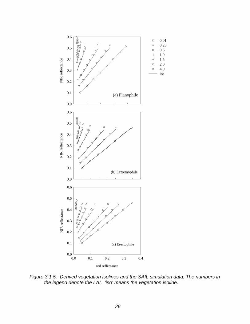
26

Figure 3.1.5: Derived vegetation isolines and the SAIL simulation data. The numbers inthe legend denote the LAI. 'iso' means the vegetation isoline.

NIR

ref

lect

ance

0.0

0.1

0.2

0.3

0.4

0.5

0.60.010.250.51.01.52.04.0iso

(a) Planophile

(c) Erectophile

red reflectance

0.0 0.1 0.2 0.3 0.4

NIR

ref

lect

ance

0.0

0.1

0.2

0.3

0.4

0.5

0.6

(b) Extremophile

NIR

ref

lect

ance

0.0

0.1

0.2

0.3

0.4

0.5

0.6

27

Comparison of vegetation indices by vegetation isoline and simulation data

The purpose of this section is to examine the accuracy of vegetation indicesobtained by using the derived vegetation isoline equation. If the isoline equation yieldsreasonably accurate vegetation index values, then we can utilize the derived analyticalrepresentation, instead of using the simulated or experimental data points, to see thevariability of vegetation indices against canopy background. The use of the vegetationisoline equation allows us to analyze the inherent behavior of these indices evenanalytically. One example would be the analytical expression of the NDVI only by thered reflectance for a fixed LAI. Using Eq. (6) after dropping the higher order interactionterm to represent the NDVI yields,

RN

RNNDVIρρρρ

+−

= (8a)

Da

Da

R

R

+++−

≈ργργ

)1(

)1(. (8b)

Since γ and D are both constant for a fixed LAI, the variation of NDVI depends on thevalue of the red reflectance unless D is equal to zero (where the NDVI isolinesbecomes identical to the vegetation isolnes). It also indicates that the variability ofNDVI with background is inherent to this index unless D is equal to zero.

In this study we also investigated the estimation of SAVI by the isoline equation.SAVI is represented by

)1( LL

SAVI RN

RN ++ρ+ρ

ρ−ρ= (9a)

)1()1(

)1(L

LDa

Da

R

R +++ρ+γ

+ρ−γ≈ , (9b)

where L is a soil-adjustment factor which is assumed to be 0.1 in this study. This factordepends on the RT model.

Figures 3.1.6 and 3.1.7 show the plots of these two indices obtained from Eqs. (8b)and (9b), which truncates the higher order interaction term, and also the results of theSAIL model (including the higher order interaction model). The agreement of these twoare good for all the cases (especially for the cases of lower background brightness).

The resulting equation effectively represents the known properties of the vegetationisoline, namely that the slope increases exponentially as LAI increases and that the Y-intercept increases to a maximum, rather than increasing monotonically. A technique tonumerically obtain such an isoline for any fixed LAI/LAD is proposed and demonstratedwith the SAIL canopy RT model (Appendix A). The technique consists of twosimulations, one with the perfect absorber as a background and the other with anarbitrary, medium to dark, background to obtain the pure vegetation canopy reflectance

28

and the average canopy transmittance. Since the above two cases are independent ofthe actual soil brightness, one does not need to know the optical properties of theactual soil. The technique involved an approximation of the hemispherical canopyreflectance (from the bottom of the canopy layer, downward) by the pure canopy(perfect absorber background) reflectance.

This work has been shown to be useful as a way to investigate the inherent variationof vegetation indices (Yoshioka, 1999). Since the characteristics of the vegetationisoline are functions of the canopy optical properties and soil line parameters, this is animportant starting point for the de-coupling of the canopy background from thevegetation layer to reduce the total number of simulations needed to obtain vegetationisolines numerically.

This approach is also significant to both the development and use of vegetationindices and to the use of canopy radiative transfer models for biophysical parameterextraction. For example, LAI retrieval by using the vegetation isolines is equivalent tofind a particular vegetation isoline that goes through the target reflectance point in thered-NIR reflectance space. The big advantage of the use of vegetation isolines is to beable to minimize the background brightness effects, since the vegetation isolineequations do not include the soil reflectances. The ultimate goal of designing VI is tobuild the one whose index isolines overlap the vegetation isolines. The derivation of thevegetation isoline equations is an indispensable step toward this goal.

29

Figure 3.1.6: NDVI vs. LAI for the soil reflectance (red) of 0.05, 0.2, and 0.35. Themarks are the SAIL model and the lines are the vegetation isolines.

(a) Planophile

ND

VI

0.0

0.2

0.4

0.6

0.8

1.0

0.05 (SAIL)0.2 (SAIL)0.35(SAIL)0.05(ISO)0.2 (ISO)0.35(ISO)

(b) Extremophile

ND

VI

0.0

0.2

0.4

0.6

0.8

1.0

(c) Erectophile

LAI

0 1 2 3 4

ND

VI

0.0

0.2

0.4

0.6

0.8

1.0

30

Figure 3.1.7: SAVI vs. LAI for the soil reflectance (red) of 0.05, 0.2, and 0.35. Themarks are the SAIL model and the lines are the vegetation isolines.

(a) Planophile

SAV

I

0.0

0.2

0.4

0.6

0.8

1.0

0.05 (SAIL)0.2 (SAIL)0.35(SAIL)0.05(ISO)0.2 (ISO)0.35(ISO)

(b) Extremophile

SAV

I

0.0

0.2

0.4

0.6

0.8

1.0

(c) Erectophile

LAI

0 1 2 3 4

SAV

I

0.1

0.2

0.3

0.4

0.5

0.6

0.7

0.8

0.9

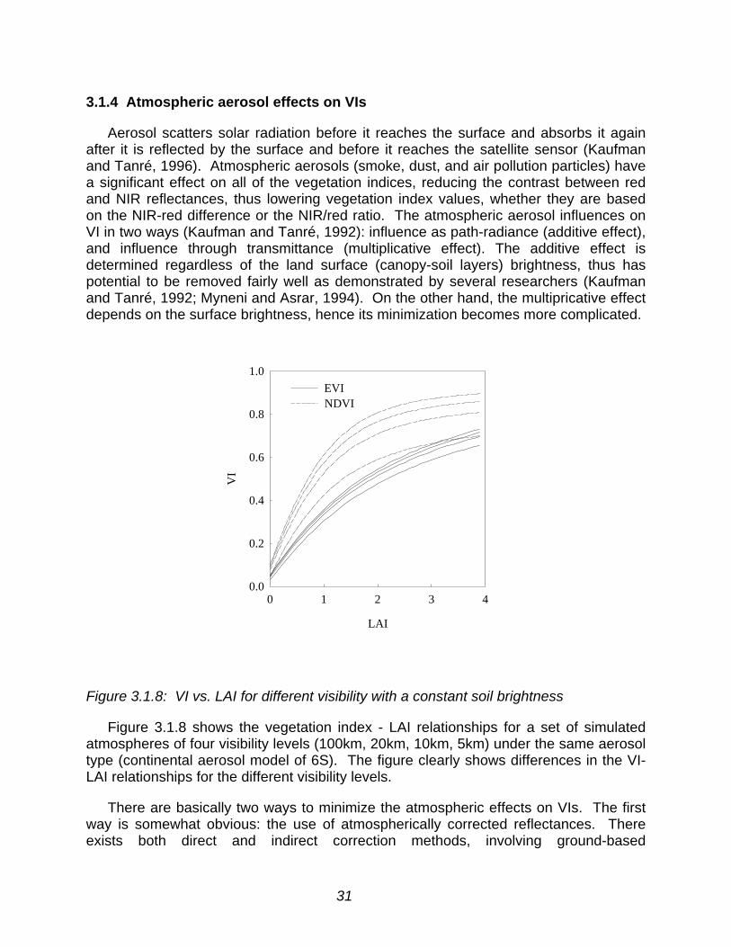
31

3.1.4 Atmospheric aerosol effects on VIs

Aerosol scatters solar radiation before it reaches the surface and absorbs it againafter it is reflected by the surface and before it reaches the satellite sensor (Kaufmanand Tanré, 1996). Atmospheric aerosols (smoke, dust, and air pollution particles) havea significant effect on all of the vegetation indices, reducing the contrast between redand NIR reflectances, thus lowering vegetation index values, whether they are basedon the NIR-red difference or the NIR/red ratio. The atmospheric aerosol influences onVI in two ways (Kaufman and Tanré, 1992): influence as path-radiance (additive effect),and influence through transmittance (multiplicative effect). The additive effect isdetermined regardless of the land surface (canopy-soil layers) brightness, thus haspotential to be removed fairly well as demonstrated by several researchers (Kaufmanand Tanré, 1992; Myneni and Asrar, 1994). On the other hand, the multipricative effectdepends on the surface brightness, hence its minimization becomes more complicated.

LAI

0 1 2 3 4

VI

0.0

0.2

0.4

0.6

0.8

1.0

EVINDVI

Figure 3.1.8: VI vs. LAI for different visibility with a constant soil brightness

Figure 3.1.8 shows the vegetation index - LAI relationships for a set of simulatedatmospheres of four visibility levels (100km, 20km, 10km, 5km) under the same aerosoltype (continental aerosol model of 6S). The figure clearly shows differences in the VI-LAI relationships for the different visibility levels.

There are basically two ways to minimize the atmospheric effects on VIs. The firstway is somewhat obvious: the use of atmospherically corrected reflectances. Thereexists both direct and indirect correction methods, involving ground-based

32

measurements, radiative transfer models, climatology, and dark object subtractionapproaches. However, to date, correction for aerosols over land has never beenachieved on an operational basis (Kaufman and Tanré, 1996) and it may not bepossible to implement a globally consistent, atmospheric correction scheme utilizingclimatology and dark object subtraction methods. The second way is to use VIs stableto the atmospheric condition variations. There has been several vegetation indexequations developed which mimimize aerosol influences indirectly on a pixel by pixelbasis. This would be useful in smoke-filled areas, where the spatial variability ofaerosols will exceed the resolution grid size of the aerosol products.

3.1.5 Atmospheric aerosol resistance in VIs

A major finding on atmospheric effect minimization is the use of the difference inblue and red reflectances as an estimator of the atmosphere influence level (Kaufman-Tanré, 1992). This concept is based on the wavelength dependency of aerosolscattering cross sections. In general the scattering cross section in the blue band islarger than that in the red band. When the aerosol concentration is higher, thedifference in the two bands becomes larger. This information is used to stabilize theindex value against variations in aerosol concentration levels. There are mainly two VIsusing the approach: ARVI and EVI.

Kaufman and Tanré (1992) developed the atmospherically resistant vegetationindex (ARVI) to minimize atmospheric-induced variations in the VI on a pixel by pixelbasis. The ARVI utilizes the difference in radiance between the blue and the redchannel, via a *

rbρ function, to correct the radiance in the red channel and stabilize theindex to temporal and spatial variations in atmospheric aerosol content:

**

**

rbN

rbNARVIρ+ρρ−ρ

= , (10)

where

)( ****RBRrb ρ−ργ−ρ=ρ , (11)

and *ρ are reflectances with prior correction for molecular scattering and ozone

absorption. The performance of ARVI depends on γ, which is determined to minimizethe path-radiance effect (Kaufman and Tanré, 1992) on *

rbρ .

The atmospheric resistance concept may also be incorporated into the SAVI to forma soil and atmospherically resistant vegetation index or SARVI (Kaufman and Tanré,1992). Liu and Huete (1994), however, found soil and atmospheric influences to beinteractive such that the removal of one source of noise increased the presence of theother. Consequently, a feedback term was utilized for simultaneous correction,resulting in an EVI formula written as:

33

)1(*

2*

1*

**

LLCC

EVIBRN

RN ++ρ−ρ+ρ

ρ−ρ= . (12)

EVI is a modified NDVI with a soil adjustment factor, L, and two coefficients, C1 and C2,which describe the use of the blue band in correction of the red band for atmosphericaerosol scattering. An example of the smoke correcting capabilities of the EVI formulais shown in Figure 3.1.9. The coefficients, C1, C2 and L, are empirically determined as6.0, 7.5 and 1.0 respectively.

Color composite NDVI EVI

Figure 3.1.9: Landsat color composite and NDVI and EVI over a vegetated area with asmoke plume.

3.2 Vegetation Index Compositing Overview

The soon to be launched MODIS-EOS (MODerate resolution ImagingSpectroradiometer - Earth Observing System; Salomonson et al., 1989, Justice et al.,1998), will acquire global bi-directional radiance data of the Earth’s surface underdifferent solar illumination angles and atmospheric conditions, e.g. clouds. In thischapter, an improved vegetation index compositing scheme will be described, whichminimizes cloud effects and angular variations due to the sun-target-sensor positions,and maximizes the global coverage. Vegetation index compositing is the process ofcombining multiple days of satellite reflectance, VI, angular and quality assurance datain an optimal manner to produce a VI image for a set temporal interval. The MODIScompositing scheme is designed to produce a spatially continuous VI image thatrepresents the composite period, while filtering out clouds and data with bad integrity.Because the daily ascending MODIS orbits do not completely overlap, especially at theequator, two days are needed to get complete global coverage. However, the mainreason why the daily orbits need to be composited over time to produce a spatiallycontinuous and consistent VI image, is the extensive cloud cover over many parts of theEarth's surface. Also, the data from some orbits will be missing due to for examplesatellite calibration maneuvers, satellite data transmission interrupts or possibly dataingest problems at receiving stations. The described MODIS compositing algorithm willprovide insight in the functioning of the algorithm and data processing aspects that were

34

taken into account to produce the VI's. Figure 3.2.1 displays a false color image of thegreen, red and NIR SeaWiFS reflectance bands for a days worth of orbits. Notice theincomplete coverage and the white cloud cover patches. The second image is acomposition of 16 consecutive days of SeaWiFS data, obtained by a MODIS likecomposite algorithm. Figure 3.2.2 shows the angular variations for several SeaWiFSorbits of one day.

The data from satellite systems, such as the AVHRR (Advanced Very HighResolution Radiometer; Agbu et al., 1994) and SeaWiFS (Sea-Viewing Wide Field-of-View Sensor; Hooker et al., 1994 were used to test and prototype the MODIS VIcompositing algorithms despite their differences in spatial and spectral resolution andorbital characteristics. The MODIS VI products will be produced at 250m, 1km and28km resolution at set temporal intervals of 16 days and 1 calendar month. The inputdata for MODIS optical bands are 250m for the red and near-infrared reflectance bandsand 500m for the blue and middle infrared bands. In the following sections the at-launch MODIS algorithms are presented with due consideration to the combinedMODIS orbital, spectral, spatial, radiometric, calibration, temporal and upstreamprocessing algorithm framework.

Beside mosaicking or compositing a set number of daily discontinuous data sets intoone representative data set or product, the effect of sun-target-sensor geometry willinfluence the results significantly and gives a need to standardize the compositedproduct as much as possible. The influence of variable sun-target-sensor configurationson derived vegetation indices can be standardized in various manners, including: (1)standardization of reflectances to nadir view angle at a solar zenith angle representativeof the observations; (2) standardization of reflectances to nadir view angle and atemporally and globally constant solar zenith angle; (3) adjustment to a constant “off-nadir” view angle with a constant sun angle; or (4) the use of spectral (bi-hemispherical)albedos. Preliminary analysis (Huete et al., 1996) suggests that both the third andfourth approaches may enhance vegetation detection only over a limited range of landcover conditions (Kimes et al., 1984; Privette et al., 1996), and will result in overalldecreased sensitivity from desert to forest, and present greater saturation problems inmore densely vegetated canopies.

35

Figure 3.2.1: False color image (top) of the red, NIR and green SeaWiFS reflectancebands for one day worth of orbits. The incomplete coverage is due to the tilt-maneuvers above the equator and the swath width. White colors are clouds andsnow/ice patches. The second image (bottom) is a composition of 16consecutive days of SeaWiFS data, obtained by a MODIS like compositealgorithm.

36

Figure 3.2.2: View and solar angular variations for several SeaWiFS orbits of one day.The right image is the color composite of red, NIR and green reflectance bands.

For the standard MODIS VI products, we propose to use the first method (Justice etal., 1998; van Leeuwen et al., 1999), and examine the other three approaches post-launch. Thus VI's will be computed after the standardization of reflectances to nadirview angle at a solar zenith angle representative of the observations. This method willinvolve the use of a BRDF model. The selection of the maximum NDVI value during a

view zenith| solar zenith | rel. azimuth | color comp.view zenith| solar zenith | rel. azimuth | color comp.

SeaWiFS Swaths

55o 0o 55o

70o

0o

-60o 0o 60oCh. 6,8,3

37

composite period, constraint by view angle conditions, will be used as a back-upmethod in case the BRDF method can not be executed due to the lack of sufficientgood quality observations.

3.2.1 MODIS VI compositing attributes

MODIS (250 m and 500 m at nadir) is a whiskbroom sensor (as well as AVHRR andSeaWiFS) causing the pixel size to increase with scan angle by as much as a factor offour. The satellite specific features associated with the spatial resolution of each pixelneed to be considered when vegetation indices (VIs) are composited over time. The 16-day repeat cycle of MODIS results in variable pixel sizes in addition to a wide range ofview and sun angles. Figure 3.2.3 shows a schematic diagram of the position of thesun and MODIS sensor and variations in view angle and pixel size. MODIS will imagethe earth’s surface over a swath width of 2330 km over sensor viewing angles of ±55°cross-track with the effective view angle on the ground being slightly larger owing to theearth’s curvature. Solar zenith angles across MODIS imagery may vary up to 20° fromedge to edge of the 2330 km swath and also vary spatially with latitude and seasonallyover the growing season. The backscatter direction of the MODIS swath has largersolar zenith angles than the forward scatter (Figure 3.2.3). The pixel size is increasingwith view angle. The pixel size becomes an important variable in evaluating anisotropicand biophysical properties of both heterogeneous and homogeneous land surfaces.This introduces a source of error in that the BRDF characteristics of large pixels are notnecessarily the same as those of small pixels (Leeuwen et al., 1997a).

After applying atmospheric corrections and processing the radiance data intosurface reflectance data, these satellite systems capture the strong anisotropicreflectance properties that vary with land cover type, relative amounts of characteristicvegetation and soil components within each pixel, and sun-earth-sensor geometry.Therefore, some knowledge of the bi-directional reflectance distribution function(BRDF) is a requirement for successful utilization of directional reflectance data andvegetation indices, and the derivation of land cover-specific biophysical parameters(Cihlar et al., 1994a). However, due to frequent cloud cover and sensor-sun-earthgeometric characteristics, the reflectance data needs to be composited in time andspace to allow for temporal and spatial continuous monitoring of vegetation dynamics.

The atmospheric correction and cloud-screening approach to be used for MODISare both significantly improved over the AVHRR approach. The experience of workingwith AVHRR data aided notably in the development of the MODIS product algorithms.In the following sections we demonstrate why the Maximum VI Value Composite (MVC)approach is less desirable for compositing MODIS data.

Fundamentally, the MVC is not appropriate for the atmospherically corrected surfacereflectance data and vegetation indices to be generated by MODIS algorithms forseveral reasons. In the EOS era, surface anisotropy and bidirectional reflectances willbecome more pronounced as a result of improved atmospheric removal algorithms(Vermote et al., 1997a, 1997b), which will accentuate differences in surfacebidirectional reflectances resulting from canopy structural influences (Cihlar et al.,

38

1994a). VIs computed from atmospherically-corrected surface reflectance data willtherefore be strongly biased toward off-nadir viewing and larger solar zenith angles,where more vegetation is viewed or illuminated by the sensor.

Figure 3.2.3: Illustration of MODIS data acquisition on the EOS-AM platform (not toscale). The bidirectional reflectance distribution function (BRDF) changes withview and sun geometry. Notice the shadow caused by clouds and canopy.MODIS pixel dimensions, cross-track and along-track, change with scan angles:0° - 250 x 250 m; 15° - 270 x 260 m; 30° - 350 x 285 m; 45° - 610 x 380 m(computed for the fine resolution red and NIR detectors; 250 m at nadir on theground).

Backscatterview zenith angle

Forward scatterview zenith angle

BRDFNa dir

range of solar zenith angles

2330 km swath descending orbit

MODIS-AM

Increasing pixel size with view angle

22s°

22v°22v°

sun

))

MODIS-AM

39

In addition, the atmospheric correction is less accurate at off-nadir view angles if thecoupling between the BRDF and the downward radiance at the surface level is nottaken into account (Vermote et al., 1997a). Pixels with off-nadir viewing angles alsohave more distortions and are coarser in size, i.e., less detail. Furthermore, the MVCmethod will overestimate NDVI values, which will result in an overestimation ofvegetation biophysical parameters and will contribute to the saturation of the NDVI.

The MVC criterion applied to MODIS data will thus result in the selection of off-nadir,distorted and less radiometrically accurate pixels, and deviate from the primary goal ofworking with the finest (nominal) resolution 250m NDVI data sets. BRDF corrections ofAVHRR reflectances to a standard nadir view angle have been shown to improve theaccuracy of the composited NDVI (Roujean et al., 1992; Cihlar et al., 1994a; Wu et al.,1995). Therefore, the MODIS compositing criteria will be weighted more toward angularconsiderations. This is done by incorporating a BRDF compositing approach, which hasthe goal to standardize the VI to nadir view and representative or constant solar angles.The MVC algorithm will be used as a ‘backup’ composite scenario in case a BRDFcorrection cannot be applied and if the MODIS atmospheric correction and the MODIScloud mask are found or reported to be inaccurate. Patchiness in the VI imagery duetwo the dual composite scenario is not expected to be more than in the current MVCcompositing schemes where angles and days selected may shift in large blocks.

3.2.2 MODIS vegetation index compositing goals and considerations

The MODIS vegetation index composite scenario was developed within the EOS(Earth Observing System) framework of providing more accurate products to monitorchanges in the Earth system.

The main MODIS VI compositing goals are to:

• provide accurate and cloud-free vegetation index (VI) imagery over set temporalintervals,

• maximize global and temporal land coverage at the finest spatial and temporalresolutions possible,

• standardize variable sensor view and sun angles,

• ensure the quality and consistency of the composited data,

• depict and reconstruct phenological variations,

• accurately discriminate inter-annual variations in vegetation.

With the fore-mentioned compositing goals in mind, the following considerations arealso of importance in the design of the MODIS vegetation index compositing algorithm:

• The pixels with the smallest view zenith angle will have the finest spatialresolution. This is 250 m for the red and NIR detectors. Realistically, the 250 mpixel size will increase to over 1 km across track at the edges of the scan (55°)and up to 500 m along track (Figure 3).

40

• Spatial degradation and blurring increase greatly with off-nadir view angles(Moody and Strahler, 1994), and off-nadir pixels will thus be more difficult toregister than nadir pixels.

• Established biophysical parameter relationships with vegetation indices arebased upon nadir-viewing angles.

• Vegetation index “saturation” problems become greater with off-nadir view andlarger solar zenith angles.

3.2.3 BRDF

Vegetation indices are affected by variations in bidirectional reflectance factors,which vary greatly as a function of sun-target-sensor geometries (Walter-Shea et al.,1997. Since the VI tends to increase with both larger view and larger solar zenithangles, the resulting variability in both view and solar zenith angles are important forinter-comparison of vegetation covers at different latitudes and in different seasons, andshould be considered in the VI compositing algorithm if we are to maintain “global” VIrobustness. BRDF model parameters can be used to normalize and interpolate thesurface reflectance to nadir view angles. However, the sun angle variability will beminimally incorporated in the BRDF correction, since the data necessary to standardizeto a certain sun angle for each composite time interval (16 days in the case of MODIS)is very limited, and thus would be less accurate outside of the observed sun anglerange. More research is needed to determine the most accurate method to extrapolatesatellite observations to a standard sun angle throughout the year. Therefore, the solarzenith and azimuth angles will be included with the composited data (reflectance andvegetation index data) to be used for post-process standardization of the vegetationindices.

Numerous canopy bidirectional reflectance distribution function (BRDF) modelshave been developed to account for the anisotropy in land reflectances as a function ofview and solar zenith angles. However, a BRDF model must be robust and operationalon a global scale. Our approach is to use the simple Walthall model (Walthall et al.,1985) to standardize the reflectance data to nadir and compute nadir-based VIs. Thishas been shown to be superior to a maximum NDVI (MVC) approach (Leeuwen et al.,1996). Cihlar et al. (1994a) successfully used the Walthall model with AVHRR data fora range of vegetation types at a regional scale. The BRDF approach estimated nadir-equivalent VIs better than the MVC, which overestimated the nadir-equivalent NDVI.

The results from the BRDF approach are also thought to best represent the state ofthe land surface by involving several cloud-free observations. However, the 16-dayrepeat cycle of MODIS can result in variable BRDF characteristics (Leeuwen et al.,1997a) because the multi-angle reflectance values are acquired from pixels that vary insize during these sixteen days (Figure 3.2.3). In this case, the uncertainty in the VI willdepend on spatial resolution and the angle-distribution at which the data was obtained,the heterogeneity of the surface area, and the choice of BRDF model (Leeuwen et al.,1997a). Increasing degradation of the spatial resolution with off-nadir view angles willminimally affect the nadir-interpolated reflectance values and resulting VI values if the

41

multi-angular observations are equally distributed in view angle space (Leeuwen et al.,1997a). Nadir-equivalent reflectance retrievals for Fallow and Aspen vegetation, usingthe Walthall model and simulated MODIS pixel size degradation for the 250 m at nadirdetectors, introduced an uncertainty in the NDVI of 0.011 and 0.008 respectively(Leeuwen et al., 1997a). Off-nadir spatial degradation will impact the MODIS 1 km andcoarser VI products less since the input to these products are based on finer resolution(250 m and 500 m) data sets that are aggregated to 1 km.

Privette et al. (1997) compared many linear models as described by Wanner et al.(1995), and found that nadir interpolation was best achieved with the Ross-thick/Li-sparse BRDF model over many vegetation types (data sets collected with thePARABOLA; Portable Apparatus for Rapid Acquisition of Bidirectional Observations ofLand and Atmosphere; Deering and Leone, 1986). Leeuwen et al. (1996) found theWalthall model to perform best for nadir-equivalent vegetation indices for mostvegetation types (Advanced Solid State Array Spectroradiometer (ASAS) data sets).The Walthall model was found to work equally well as Roujean’s BRDF model. TheRoss-thick/Li sparse BRDF model caused a few outliers when used in the forwardmodeling mode to derive nadir reflectance values. Experience with ASAS and AVHRRdata showed the Walthall model to be more robust than most of the other linearmodels. The Walthall model also requires the least number of floating operations perpixel, which is an important consideration in the production of a global VI product at 250m resolution and 16-day temporal intervals.

3.2.4 Compositing period

Variable composite periods have been used to obtain cloud free NDVI data on aglobal scale. The minimum compositing period is limited by cloud cover frequency andmay vary from every 5 days at higher latitudes to as long as 30 days or more in somehumid tropical areas. NDVI composite periods have varied among 7, 9, 10, 11 and 14days and monthly intervals with variable (1 km to 1°) spatial resolutions (Townshend,1994). The composite period depends on its application and the availability of cloudfree data on a global scale. Shorter compositing periods will pick up more dynamic landcover changes and allows one to combine compositing periods to monthly or bi-weeklyperiods. However, the shorter the compositing period, the greater the likelihood ofcloud-affected or missing pixels in the composited image. The 16-day MODIScompositing cycle was designed according to the EOS-AM1 16-day repeat cycle andconsequent attainment of the full array of viewing angles. This seems appropriate sinceit provides the opportunity to avoid clouds as well as to cover all latitudes within a rangeof small viewing angles. The monthly compositing cycle is based on demand andheritage of the user community.

It is unclear if the nadir AVHRR repeat cycle of approximately 9 days versus the 16days of MODIS will affect the derivation of nadir-equivalent reflectance values fromBRDF models for either sensor. Based on the repeat cycle, more nadir AVHRR thennadir MODIS observations are possible within a 16-day period. The 2700km swathwidth of AVHRR will result in a larger view angle range compared to the 2330km swathwidth of MODIS. Furthermore, the AM overpass of MODIS results in less cloud cover in

42

comparison to the cloudier afternoon overpass of the AVHRR. Since data from bothsensors will have random dropouts of observations due to clouds, the distribution andrange of view angles will be different, but not likely to affect the final nadir-equivalent VIproduct significantly. The expected retrieval accuracy of bidirectional reflectance valuesover land for MODIS angular sampling are reported by Lucht (1998) and Wanner et al.(1997).

3.2.5 MODIS data stream

MODIS input products that are relevant to the vegetation index are shown in Figure3.2.4. The MODIS data streams (top of the atmosphere (TOA) calibrated radiance,cloud mask, atmospheric correction and surface reflectance, vegetation indices) is setup to flow into the product algorithms in a predetermined order. For a tractable and bestsolution to the compositing algorithm it was logical to input the atmosphericallycorrected surface reflectance data in combination with the cloud mask and use as many“good” observations as possible during a composite period. This runs counter to theMVC scenario based on non-atmospherically corrected reflectance data as suggestedby Cihlar et al. (1994a) for the AVHRR data. If changes in the vegetation indexcompositing algorithm call for a different processing scenario, significant changes in theEOS production system can be required, including hardware, software and networkingredesign and implementation.

43

Figure 3.2.4: Flow diagram showing the relationship of relevant MODIS Land andAtmosphere Products (Level 1-L1; Level 2 - L2; Gridded L2-L2G; Level 3 - L3)that are required to generate the gridded, composited vegetation indices.

3.2.6 MODIS VI composite algorithm

The logic of the compositing algorithm is based on the MODIS specific input dataand theoretical knowledge of radiative transfer and surface reflectance anisotropy. Thecompositing algorithm will optimize the choice of the best VI representative for each

44

composite period, spatial resolution and global land extent. The compositing algorithmswill rely on information from the cloud mask (Ackerman et al., 1996), atmosphericcorrection (Vermote, 1997a), view zenith angle, solar zenith angle, relative azimuthangle, geo-registration (Wolfe et al., 1998), and surface BRDF normalization. Thealgorithms utilize the information in the reflectance-quality assurance (QA) flags,partially derived from the MODIS cloud mask product, to pre-process theatmospherically corrected reflectance data of MODIS bands 1, 2, and 3 and 7 (red,NIR, blue, MIR) over land only. Land pixels with clouds, shadow, and bad data integritywill be excluded from the VI composite.

The MODIS algorithm selects all the reflectance data for a 16-day period, based ondata integrity and cloud flags, and fits the Walthall BRDF model to the individual banddata. The empirical BRDF model developed by Walthall et al. (1985), is used to derivenadir reflectance data for each pixel and 16-day intervals:

λλλλ +φ−φθ+θ=φφθρ c)cos(a),,( svv2vvsv b (13)

where the atmospherically corrected reflectance (ρλ) values for the appropriatewavelengths (λ; i.e. red, NIR, blue) are modeled as a function of the view zenith angle(θv), and sun (φs) and view (φv) azimuth angles. The model parameters aλ, bλ and cλ areobtained using a least squares curve fitting procedure. “cλ” is equal to the reflectance atnadir view angle. The prevalent sun angle and VIs will be computed from thecomposited and normalized surface reflectance observations. Based on our experiencewith AVHRR and ASAS data, a minimum of 5 surface reflectance observations arecurrently required for a stable BRDF model (Walthall’s) inversion. Nadir interpolatedvalues will be rejected when the resulting reflectance values are negative or when theNDVI is higher or much lower than the MVC based NDVI (0.3-NDVI MVC <= NDVIBRDF <=NDVI MVC+0.05). These thresholds are set to avoid the inclusion of residual cloudeffects resulting in the BRDF results to be off. If observations during a 16-day intervalare unequally distributed in view angle space (e.g. backscatter observations only) orunequally affected by undesirable atmospheric conditions (e.g. smoke, clouds),negative nadir reflectance values can be derived from the BRDF model. Negativereflectance values can also be generated if inaccurate atmospheric parameters (e.g.aerosol optical thickness) are used to realize atmospheric corrections.

Since not all pixels will have 5 or more cloud-free data points during a 16-dayperiod, a back-up algorithm is used which selects the highest NDVI based on two cloud-free pixels with their view angles closest to nadir. The absolute view zenith angle istaken for all cloud-free pixels after which their view angles are sorted in ascendingorder. The NDVI is computed for the observations with the two smallest view zenithangles, after which the MVC rule is applied and the most optimal observation selected.This will be referred to as the constraint view angle maximum value composite (CV-MVC) approach. If only one cloud-free observation is available over the compositeperiod, this observation will automatically be selected to represent the compositeperiod. If all data during a 16-day period were affected by clouds, based on the cloudflags, the view angle constraint for the MVC method will be released and the VI will becalculated for all days and the best pixel chosen based on the maximum value of the

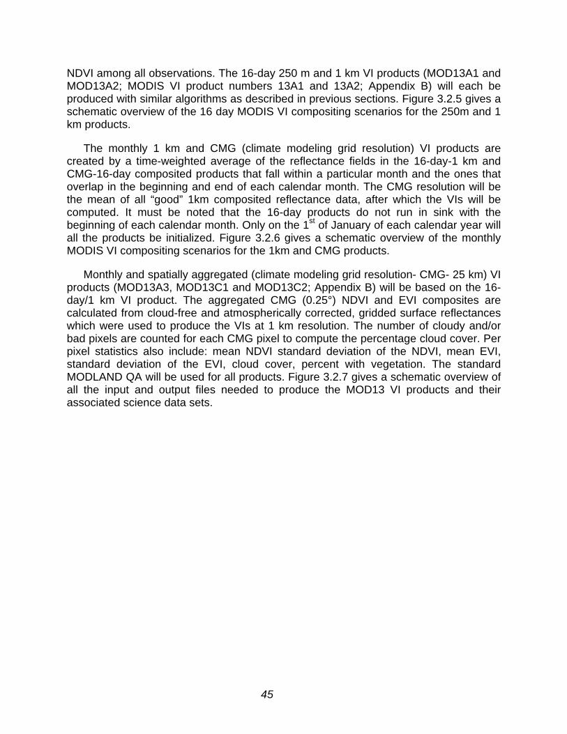
45

NDVI among all observations. The 16-day 250 m and 1 km VI products (MOD13A1 andMOD13A2; MODIS VI product numbers 13A1 and 13A2; Appendix B) will each beproduced with similar algorithms as described in previous sections. Figure 3.2.5 gives aschematic overview of the 16 day MODIS VI compositing scenarios for the 250m and 1km products.

The monthly 1 km and CMG (climate modeling grid resolution) VI products arecreated by a time-weighted average of the reflectance fields in the 16-day-1 km andCMG-16-day composited products that fall within a particular month and the ones thatoverlap in the beginning and end of each calendar month. The CMG resolution will bethe mean of all “good” 1km composited reflectance data, after which the VIs will becomputed. It must be noted that the 16-day products do not run in sink with thebeginning of each calendar month. Only on the 1st of January of each calendar year willall the products be initialized. Figure 3.2.6 gives a schematic overview of the monthlyMODIS VI compositing scenarios for the 1km and CMG products.

Monthly and spatially aggregated (climate modeling grid resolution- CMG- 25 km) VIproducts (MOD13A3, MOD13C1 and MOD13C2; Appendix B) will be based on the 16-day/1 km VI product. The aggregated CMG (0.25°) NDVI and EVI composites arecalculated from cloud-free and atmospherically corrected, gridded surface reflectanceswhich were used to produce the VIs at 1 km resolution. The number of cloudy and/orbad pixels are counted for each CMG pixel to compute the percentage cloud cover. Perpixel statistics also include: mean NDVI standard deviation of the NDVI, mean EVI,standard deviation of the EVI, cloud cover, percent with vegetation. The standardMODLAND QA will be used for all products. Figure 3.2.7 gives a schematic overview ofall the input and output files needed to produce the MOD13 VI products and theirassociated science data sets.

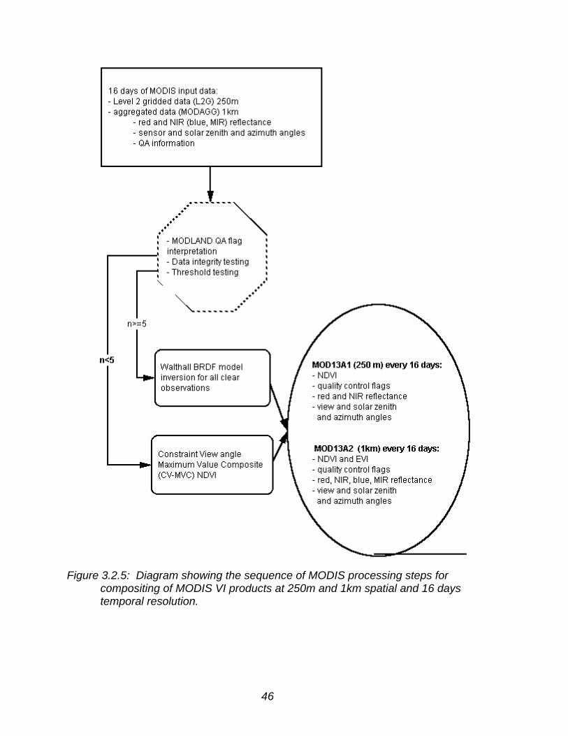
46

Figure 3.2.5: Diagram showing the sequence of MODIS processing steps forcompositing of MODIS VI products at 250m and 1km spatial and 16 daystemporal resolution.

47

Figure 3.2.6: Diagram showing the sequence of MODIS processing steps for thecompositing of monthly MODIS VI products at 1km and 25km spatial resolution.

48

Figure 3.2.7: Schematic overview of all the input files needed to produce the MOD13VI products and their associated science data sets.

49

3.2.7 Pre-launch MODIS VI prototypes

AVHRR Pathfinder data

One year (1989) of daily Pathfinder AVHRR data over land (James and Kalluri,1994) was obtained from the GSFC-DAAC (Goddard Space Flight Center- DistributedActive Archive Center) to test and prototype the MODIS vegetation index compositing(van Leeuwen et al., 1999). The daily Pathfinder data is mapped to a global 8 km equalarea grid using the Goode Interrupted Homolosine projection, resulting in global spatialdimensions of 5004 by 2168 pixels (columns and rows). The AVHRR data was in theHierarchical Data Format (HDF) and consisted of twelve data fields: NDVI, CLAVR(cloud algorithm for AVHRR) cloud flags, Quality assurance flags, Scan angle, Solarzenith angle, Relative azimuth angle, Channel 1 reflectance, Channel 2 reflectance,Channel 3 brightness temperature, Channel 4 brightness temperature, Channel 5brightness temperature, Date and hour of the observation. The reflectance data wasalready corrected for Rayleigh scattering and ozone absorption. Cloud flags wereproduced by NOAA’s cloud algorithm for AVHRR (CLAVR; Stowe et al., 1991). Theland/sea mask was an ancillary data layer used in the processing. More specificinformation on the Pathfinder AVHRR land data can be found in the User’s manual(Agbu and James, 1994).

AVHRR temporal VI profiles

Applying the MODIS and MVC compositing algorithms to 1 year of daily AVHRRdata resulted in twenty-three consecutive global composites of the NDVI. The meanglobal NDVIMODIS and NDVIMVC values were obtained for all pixels, composite periodsand different MODIS compositing scenarios. Globally, the NDVIMODIS was between 5 to8 % lower then the NDVIMVC. Using the QA information, for each pixel where the BRDFmodel was applied, the MVC was computed as well and the relative differencecomputed for these pixels. Whenever the MODIS-BRDF was applied, the resultingNDVI values were between 20 to 30% lower than the NDVIMVC (van Leeuwen et al.,1999). Figure 3.2.8 shows seasonal profiles of the NDVIMODIS for each continent. Thepeak of the growing season is different for each continent. The relative differences [100(NDVIMVC - NDVIMODIS) / NDVIMVC] were computed for each continent and rangedbetween 1 and 24 % for all 16-day composite periods during the 1989 AVHRRobservations (Leeuwen et al., 1997b).

50

133

6597

129161

193225

257289

321353

DOY

0

0.1

0.2

0.3

0.4

0.5

ND

VI

Africa

Asia

Australia

Europe

NorthAmerica

SouthAmerica

Figure 3.2.8: Continental NDVI profiles for the MODIS composite algorithm; AVHRR(8km).

Desert and deciduous broadleaf forest temporal VI profiles

The relative accuracy of the MODIS-BRDF algorithm was evaluated throughtemporal NDVI, red and NIR value profiles from pixels extracted from Desert andDeciduous Broadleaf Forest (Figure 3.2.9 and Figure 3.2.10). The compositedreflectance data is utilized in VI computation and is also output with the VI, providingadditional data fields for vegetation studies. Figure 9a shows an example of a seasonalNDVIMODIS and NDVIMVC profiles, with the NDVIMODIS being equal or slightly lower thenthe NDVIMVC. NDVIMODIS profiles are slightly smoother than the NDVIMVC profiles (Figs.3.2.9a and 3.2.10a,b). The temporal red and NIR reflectance profiles (Figure 3.2.9b)are following the same trend for both MVC and MODIS composite methods. Thecombination of MODIS BRDF and CV-MVC composite methods performed well.

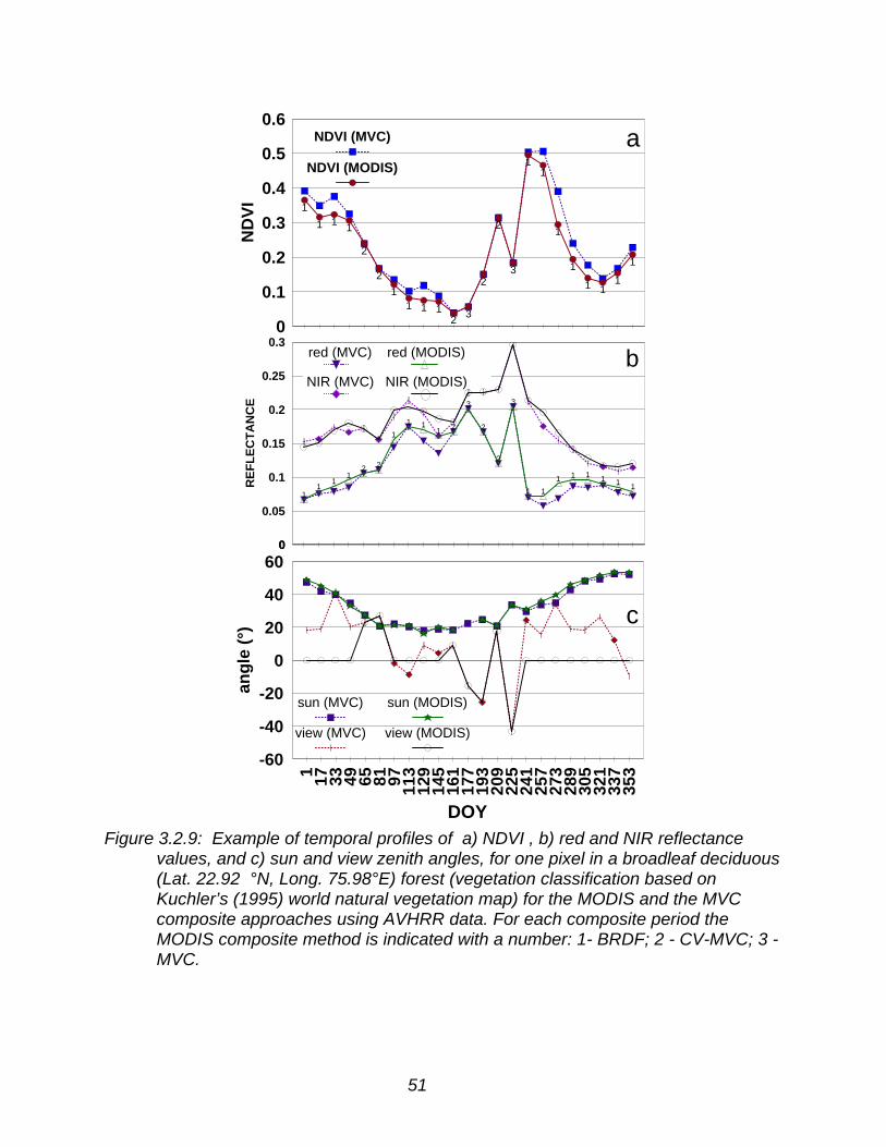
51

1

1 1 1

2

2

11 1 1

2 3

2

2

3

11

1

1

1 11

1

0

0.1

0.2

0.3

0.4

0.5

0.6

ND

VI

NDVI (MVC)

NDVI (MODIS)

1 17 33 49 65 81 97 113

129

145

161

177

193

209

225

241

257

273

289

305

321

337

353

DOY

-60

-40

-20

0

20

40

60

ang

le (

°)

sun (MVC)

view (MVC)

sun (MODIS)

view (MODIS)

a

c

11

11

2 2

1

1 11 2

3

2

2

3

1 1

1 1 1 1 1 1

0

0.05

0.1

0.15

0.2

0.25

0.3

0

RE

FL

EC

TA

NC

E

bred (MVC)

NIR (MVC)

red (MODIS)

NIR (MODIS)

Figure 3.2.9: Example of temporal profiles of a) NDVI , b) red and NIR reflectancevalues, and c) sun and view zenith angles, for one pixel in a broadleaf deciduous(Lat. 22.92 °N, Long. 75.98°E) forest (vegetation classification based onKuchler’s (1995) world natural vegetation map) for the MODIS and the MVCcomposite approaches using AVHRR data. For each composite period theMODIS composite method is indicated with a number: 1- BRDF; 2 - CV-MVC; 3 -MVC.

52

48° 44

° 38

° 33

° 28° 24

° 21

° 22°

19°

19°

21°

20°

20°

24°

26°

29°

35°

40°

45°

50°

51°

53°

53°

1 1 2 1 1 1 1 1 1 1 1 1 1 1 1 1 1 1 1 21 1 1

1 17 33 49 65 81 97 113

129

145

161

177

193

209

225

241

257

273

289

305

321

337

353

DOY

0

0.1

0.2

0.3

0.4

0.5

ND

VI,

RE

FLE

CT

AN

CE

NDVI

RED

NIR

48°

43°

40°

31° 29

° 20°

21° 25

°

17°

21° 14

°

20°

20°

17°

21°

35°

29°

40°

44°

44°

52°

51° 52

°

6°

34°

7° -

23°

-21

°

30°

2°

-36

°

17°

-9° 3

6°

6°

-22

°

31°

17°

13°

28°

17°

23°

30° 7

°

26°

20°

1 17 33 49 65 81 97 113

129

145

161

177

193

209

225

241

257

273

289

305

321

337

353

DOY

0

0.1

0.2

0.3

0.4

0.5

ND

VI,

RE

FLE

CT

AN

CE

NDVI

RED

NIR

view zenith angles

sun zenith angles

sun zenith angles

composite method

a) MVC

b) MODIS

Figure 3.2.10: Example of temporal profiles of NDVI, red and NIR reflectance valuesfor one desert vegetation pixel (Lat. 22.0°N, Long. 27.15°E) (vegetationclassification based on Kuchler’s (1995) world natural vegetation map) for the a)MVC and b) MODIS composite approaches using AVHRR data. For eachcomposite period the MODIS composite method is indicated with a number: 1-BRDF; 2 - CV-MVC. The sun zenith angle and view zenith angle are also shownfor each composite period. The negative and positive view angles are indicatedfor the respective backscatter and forward scatter view direction. The view zenithangle for the MODIS-BRDF corrected data is 0°.

53

Prototype of MODIS VI imagery

Figures 3.2.11 and 3.2.12 are prototype images of the global MODIS-NDVI and QAproduct for one 16-day composite period. The combination of MODIS BRDF and CV-MVC (constraint view angle maximum value composite) composite methods performedwell. Obvious discontinuities or artifacts due to the combined use of two to threecomposite methods were not observed. The pseudo color image of the NDVI allows forfast visual examination of vegetation density and photosynthetically active regions ofthe world. The associated pseudo color quality assurance (QA) image permits forquality checks of the algorithm, cloud cover persistence and examination of region withmissing data.

Temporal and spatial VI trend analysis will be a powerful tool to detect effects ofclimate change and monitor vegetation dynamics. Note that the BRDF correction islimited to the semi-arid/arid regions, where cloud cover is less persistent than overother regions of the world. It is likely that the cloud cover will be less for the AMoverpass time of MODIS in comparison with the afternoon overpass time of AVHRR.Consequently, the BRDF correction will be more frequently applied relative to theAVHRR PM data.

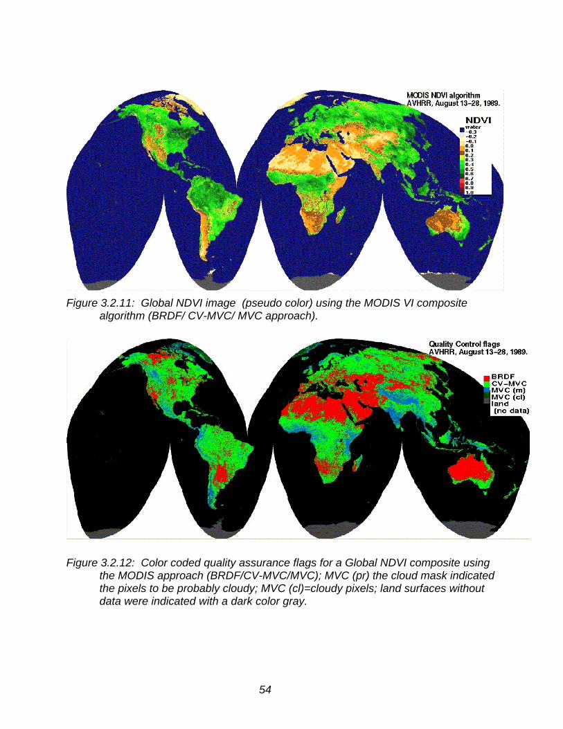
54

Figure 3.2.11: Global NDVI image (pseudo color) using the MODIS VI compositealgorithm (BRDF/ CV-MVC/ MVC approach).

Figure 3.2.12: Color coded quality assurance flags for a Global NDVI composite usingthe MODIS approach (BRDF/CV-MVC/MVC); MVC (pr) the cloud mask indicatedthe pixels to be probably cloudy; MVC (cl)=cloudy pixels; land surfaces withoutdata were indicated with a dark color gray.

55

AVHRR view angle distribution

The benefit of the MODIS compositing approach is noticeable by the smaller orequal view angles and the associated smaller pixel sizes. The view angle distribution ofthe MVC algorithm is more biased towards the forward scatter direction than the viewangle distribution of the MODIS algorithm (Figure 3.2.13). The strong peak at nadir viewangles is due to the BRDF standardization of the reflectance factors to nadir. The viewangle distribution of the CV-MVC algorithm is also less biased towards the forwardscatter (positive angles) in comparison with the MVC algorithm as shown in Figure3.2.13

Figure 3.2.13: Global view angle distribution (including all continents) for a 16-daycomposite period (August 13-August 28, 1989) for the MODIS (BRDF/CV-MVC)and CV-MVC and MVC algorithms.

SeaWiFS prototype

One set of 16 days of continuous global SeaWiFS (Sea-viewing Wide Field-of-viewSensor) reflectance (surface reflectance data corrected for Rayleigh scattering, Ozoneand water vapor) and sun-sensor geometry data (5000 columns x 2500 rows; 8 kmspatial resolution; for 16 days during 1997; September 15 to October 1; Sept. 17 datawere missing; Robinson projection) were used to test and prototype the MODISvegetation index compositing algorithms. The SeaWiFS vegetation index data werecomposited in space and time to monitor vegetation changes in a spatial continuousfashion.

The SeaWiFS was tilted 20°, preventing nadir looks of the Earth's surface. Ascanner tilt mechanism enables the instrument to be oriented in the along-track

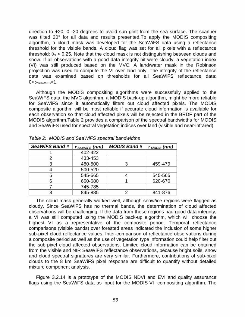
56

direction to +20, 0 -20 degrees to avoid sun glint from the sea surface. The scannerwas tilted 20° for all data and results presented.To apply the MODIS compositingalgorithm, a cloud mask was developed for the SeaWiFS data using a reflectancethreshold for the visible bands. A cloud flag was set for all pixels with a reflectancethreshold: θ3 > 0.25. Note that the cloud mask is not distinguishing between clouds andsnow. If all observations with a good data integrity bit were cloudy, a vegetation index(VI) was still produced based on the MVC. A land/water mask in the Robinsonprojection was used to compute the VI over land only. The integrity of the reflectancedata was examined based on thresholds for all SeaWiFS reflectance data:0<ρSeaWiFS<1.

Although the MODIS compositing algorithms were successfully applied to theSeaWiFS data, the MVC algorithm, a MODIS back-up algorithm, might be more reliablefor SeaWiFS since it automatically filters out cloud affected pixels. The MODIScomposite algorithm will be most reliable if accurate cloud information is available foreach observation so that cloud affected pixels will be rejected in the BRDF part of theMODIS algorithm.Table 2 provides a comparison of the spectral bandwidths for MODISand SeaWiFS used for spectral vegetation indices over land (visible and near-infrared).

Table 2: MODIS and SeaWiFS spectral bandwidths

SeaWiFS Band # ρρSeaWiFS (nm) MODIS Band # ρρMODIS (nm)1 402-4222 433-4533 480-500 3 459-4794 500-5205 545-565 4 545-5656 660-680 1 620-6707 745-7858 845-885 2 841-876

The cloud mask generally worked well, although snow/ice regions were flagged ascloudy. Since SeaWiFS has no thermal bands, the determination of cloud affectedobservations will be challenging. If the data from these regions had good data integrity,a VI was still computed using the MODIS back-up algorithm, which will choose thehighest VI as a representative of the composite period. Temporal reflectancecomparisons (visible bands) over forested areas indicated the inclusion of some highersub-pixel cloud reflectance values. Inter-comparison of reflectance observations duringa composite period as well as the use of vegetation type information could help filter outthe sub-pixel cloud affected observations. Limited cloud information can be obtainedfrom the visible and NIR SeaWiFS reflectance observations, because bright soils, snowand cloud spectral signatures are very similar. Furthermore, contributions of sub-pixelclouds to the 8 km SeaWiFS pixel response are difficult to quantify without detailedmixture component analysis.

Figure 3.2.14 is a prototype of the MODIS NDVI and EVI and quality assuranceflags using the SeaWiFS data as input for the MODIS-VI- compositing algorithm. The

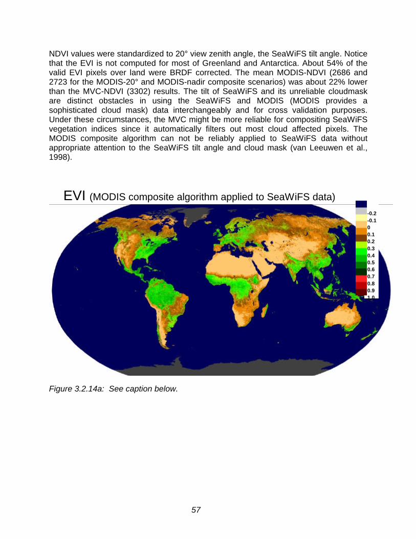
57

NDVI values were standardized to 20° view zenith angle, the SeaWiFS tilt angle. Noticethat the EVI is not computed for most of Greenland and Antarctica. About 54% of thevalid EVI pixels over land were BRDF corrected. The mean MODIS-NDVI (2686 and2723 for the MODIS-20° and MODIS-nadir composite scenarios) was about 22% lowerthan the MVC-NDVI (3302) results. The tilt of SeaWiFS and its unreliable cloudmaskare distinct obstacles in using the SeaWiFS and MODIS (MODIS provides asophisticated cloud mask) data interchangeably and for cross validation purposes.Under these circumstances, the MVC might be more reliable for compositing SeaWiFSvegetation indices since it automatically filters out most cloud affected pixels. TheMODIS composite algorithm can not be reliably applied to SeaWiFS data withoutappropriate attention to the SeaWiFS tilt angle and cloud mask (van Leeuwen et al.,1998).

EVI (MODIS composite algorithm applied to SeaWiFS data)

-0.2-0.100.10.20.30.40.50.60.70.80.91.0

Figure 3.2.14a: See caption below.

58

Figure 3.2.14: Global EVI (a) and NDVI (b) image (pseudo color) using the MODIS VIcomposite algorithm (BRDF/ CV-MVC/ MVC approach). (c) Color coded qualityassurance flags for a Global NDVI composite (very similar for EVI) using theMODIS approach (BRDF/CV-MVC/MVC)

59

Figure 3.2.15: SEAWIFS color composite, NDVI, EVI and view angle distribution forSouth America.

Figure 3.2.15 shows a SEAWIFS color composite with some slight traces of smoke andclouds still visible. The NDVI and EVI have different dynamic ranges. The view angledistribution for South America shows that large areas where standardized by using aBRDF based compositing approach.

60

3.2.8 Alternative VI compositing approaches

The MODIS/MISR BRDF production scheme will generate BRDF parameters andalbedo every sixteen days with a 1 km spatial resolution with a required minimum of tencloud-free observations to be reliable (Strahler et al., 1996). The MODIS BRDFdatabase is currently incompatible with the needs of the 250m gridded MODIS NDVIproduct due to the coarser spatial and temporal resolutions of the BRDF product. Sincethe MODIS VI compositing algorithm has the specific aim of deriving nadir equivalentreflectance values, and not the complete BRDF (needed for albedo), five observationsare considered sufficient for nadir interpolation. The feasibility of applying the BRDFproduct (1 km) to finer resolutions (250 m) (sharpening mode of the BRDF product) wasinvestigated by Leeuwen et al. (1997a) showing promising results for relativelyhomogeneous land cover types. The use of previous composite BRDF results or ahistoric BRDF data base is also being investigated for situations where it is impossibleto derive nadir reflectance values due to a limited number of observations (Leeuwen etal, 1997a; Wanner et al., 1997; Lucht et al, 1999).

Standardization of VI to nadir view and a certain sun angle is being investigated fora monthly CMG VI product. Monthly compositing would ensure sufficient input data forBRDF determination using inversion of a simple BRDF model (Rahman’s; Rahman etal., 1993). The VI would be globally normalized to a constant solar-view geometry(possibly determined by the angle most sensitive to canopy biomass) at 0.25° spatialresolution (25 km). At the lower temporal resolution, this product would be cateredtowards modelers and those doing inter-annual comparisons. Local/regional workdemanding more frequent data would probably rely on the 16 day level 3 VI as planned.

A second approach to NDVI values for variations in solar zenith angles is by usingempirical relationships between the NDVI and solar zenith angle for a range of biomes.These empirical relationships can be established through in situ nadir radiometricmeasurements for a range of sun amgles. Table 3 shows a range of the expectedvariation in sun angle for low and high latitudes.

Table 3: The maximum and minimum mean solar zenith angles for land and thedifferent continents based on the AVHRR composited data. As expected, theapproximate Day of Year (DOY) the minimum and maximum sun angles occur,are during spring and fall.

Continents Sun angle (°)All (Global) 33° 53°South America 46° 33°North America 30° 67°Europe 28° 66°Australia 51° 32°Asia 27° 62°Africa 26° 46°DOY 161 337

61

3.2.9 VI compositing conclusions

Because reflectance properties of the land surface are anisotropic in nature,vegetation indices, derived from bi-directional reflectance values, are strongly affectedby the angular properties at which the target was viewed and illuminated. Retrieval ofthe bidirectional reflectance distribution function and angular standardization of thesereflectance data are essential for the proper interpretation of vegetation index data andtheir derived parameters.

The improved capabilities of MODIS will offer the opportunity to cross-validate thehistorical and ongoing AVHRR-NDVI time series (since 1982) with the MODIS-NDVItime series. Especially the differences between the AVHRR and MODIS sensors in thespectral, radiometric, and spatial domain need to be translated to meet the needs ofglobal change research. Biophysical parameters such as percent cover, biomass,fAPAR and LAI, have been derived from the NDVI measured at variable view and sunangles. Standardizing these angular effects will also allow for more accurate derivationsof biome specific or global biophysical parameters from VIs. The EVI was successfullyprototyped on a global scale with SeaWiFS data because it included a blue band. TheEVI will extend sensitivity into dense vegetation types such as forests and agriculturalareas while reducing the noise effects of canopy background and atmospheric aerosols(Justice et al., 1998).

There is some concern that the MODIS compositing approach, a combination of theBRDF and back-up MVC (maximum value composite) methods, will affect data purityand cause more discontinuities on a regional scale than a single criteria compositemethod (e.g. MVC). At this point, the MODIS approach has the advantage over theMVC approach through standardization of view angles and emphasis on the selectionof nadir (finest spatial resolution) observations. However, the MODIS approach is moreadversely affected by cloud and atmospheric effects than the MVC. The selection of themaximum NDVI tends to mask the natural vegetation variations in more denselyvegetated areas due to saturation effects. A final evaluation of the MODIS compositeapproach will be based on the quality of the actual MODIS data, product evaluationsand user community requirements.

Since many uncertainties remain as to how the actual MODIS instrument and thedeveloped algorithms are going to perform, some flexibility is being built into the currentMODIS VI compositing algorithm, that allows for unexpected (e.g. unreliable geo-registration, cloud mask and atmospheric correction) data input flows. The compositingalgorithm thresholds and parameters can be relaxed or tightened depending on thequality of the data. For instance, immediately after launch, the BRDF module of thecompositing algorithm can be switched off to accommodate less ideal data due tounsuccessful cloud-masking or inaccurate day to day geo-registration. The quality ofthe MODIS data processing algorithms and the MODIS specific spatial, temporal,spectral and radiometric quality of the data after the initial post launch processing willgreatly determine if all the MODIS compositing goals can be achieved.

62

• The following conclusions can be drawn based on prototyping the MODISvegetation index approach with AVHRR and SeaWiFSdata:

• A simple BRDF model and few observations (�5) per pixel were needed tostandardize the NDVI and EVI to nadir view angles and thus improve theinterpretation of the anisotropic VIs.

• The Walthall BRDF model was successfully used in prototyping global MODIS-EOS/NDVI composite scenarios with AVHRR and SeaWiFS data.

• Results of a BRDF approach are more representative of vegetation changesover a 16-day period than the MVC approach, because it incorporates all ‘good’observations and changes during a 16-day period.

• The present MODIS-BRDF composite scenario automatically extrapolates tofiner (nadir) spatial resolutions.

• A reliable cloud-mask is crucial to the BRDF-component of the MODIScompositing algorithm to exclude observations of cloud affected pixels.

• A backup composite algorithm was needed for the pixels with a limited number of“good” observations since the BRDF model can not be reliably inverted if theEarth’s surface is frequently covered with clouds.

• On a continental scale, the MVC based NDVI values were 1-30% higher than theNDVI values derived from the MODIS algorithm.

Since the vegetation indices are radiometric measures of the spatial and temporalvariations of vegetation biophysical properties, validation activities will focus on therelationship of the radiometric and biophysical changes of the land surface andincorporate multi-angular measurements as well. Research and validation activities arein progress to demonstrate the utility of the MODIS vegetation indices to improve theunderstanding of the Earth system and its dynamics due to interactions betweenclimate and land processes and human activity.

3.3 MODIS VI Quality Assurance (QA)

The quality of the vegetation index (VI) products will be assessed regularly tomonitor the accuracy and integrity of the data products over long time frames that are ofcritical importance to studies of global change and climate. Run time and post-production QA evaluations will take place at the TBRS-SCF (Terrestrial Biophysics andRemote Sensing - Science Computing Facility) and the LDOPE (Land Data OperationalProduct Evaluation) Facility at GSFC (Goddard Space Flight Center). The LDOPE willfocus mostly on day to day operational QA, while the SCF will focus more on in-depthQA analysis and product validation related to science questions. Although only afraction of the total amount of data need to be put through the SCF and LDOPE,automation of the QA procedures will be optimized as much as possible to cope withthe vast amounts of data. It is assessed that the input data stream to the TBRS-SCFwill be 2.0 GB/day. This is an average data stream, but it is expected that peak volumescould approach 24 GB per day due to the fact that 16 days of input data are needed todo the in-depth QA analysis on the 250 m VI product and its input products.

63

3.3.1 QA definition and scope

Definition of Quality Assurance (QA): Flag data products in operational mode whichdo not conform to the expected accuracies of that product, and store operationalproduction system information/data that is useful for post production quality assurance.

QA results will be derived for each pixel by (QA science data set) :

• examination of the input and output data (reflectance, VI, view-sun geometry andQA-flags) in spatial and temporal domain

• science decision making represented by the options inside the coded algorithms

• accuracy estimates derived from input and output data QA flags and systemnoise and algorithm specifications

• validation of the vegetation indices at validation sites (specific goals)

QA results will be derived for each tile by (metadata stored in the HDF file):

• summary of critical per pixel QA over the tile (e.g. MODLAND QA and summarystatistics)

• monitoring the computational and production stability of the code.

• flagging of a state or condition related to the run time production.

• accumulating and summarizing the QA of all files used in the production of a tile

• generalized accuracy estimates derived from input and output data QA flags andsystem noise and algorithm specifications

• documentation of the code versions and processing history of the data products

Anticipated quality related problems for VI products are related to three categories:

Product (output) and Input science data sets and metadata:

• VI product data integrity (check against product spec) and validity (missingtiles, beyond logical/acceptable thresholds)

• Input data integrity and its validity (missing tiles, beyond logical/acceptablethresholds)

Vegetation Index Science Issues:

• Reflectance standardization using BRDF and CV_MVC (spatial and temporal)

• Code evaluation to fine tune some of the threshold values set inside the codeto catch outliers

Software change issues:

• Software problem at SDST or SCF components,

• Processing environment

64

• Program performance

Several choices of action can be entertained based on the results of the performedQA analysis. The first two action items are related to metadata fields and have to be setfor each tile that has been or is being investigated. It is also possible to set these flagsbased on an inferred qualification from the actually investigated tiles. Paths of actionbased on QA results:

1. Set science quality flag

2. Set science quality flag explanation

3. Operational work-around or fix

4. Discontinue or decrease production

5. Develop a plan to fix the problem

Thus, the QA (quality assurance) analysis can result in algorithm and metadataadjustments. The QA analysis allows us to accumulate science quality output analysisto make informed decision on code adjustments (data base). A plan of implementationneeds to be developed to incorporate minor and major code changes. The set up of aweb site with QA results and a reference with the science quality flag explanation mightbe necessary. It is important to keep in mind that QA = “pass” or approvals from SCF’sor LDOPE will propagate to upstream products. On the other hand: QA = “fail”,problems and code changes propagate to downstream products. It is envisioned thatthe QA and validation efforts will be strung together to make efficient use of limitedresources (personnel and hardware) at the SCF. The QA and validation efforts willconsist of:

1. In depth QA analysis of 1 land tile per composite period requiring access toall input files (chosen from the validation site list). These QA activities will bemostly interactive.

2. Continuous QA and trend analysis for 50 validation sites using subsets of upto 50 land tiles and the 16-day composited VI products. These QA activitieswill be mostly automated.

3. QA analysis of spatially continuous data on a global scale (4 times per year)using 16-day composites

4. Ad hoc QA analysis of land tiles based on LDOPE or MODLAND teamfindings

3.3.2 MODIS 13 product formats and QA related metadata and science data sets

Appendix B gives an overview of MODIS 13 VI products, data field descriptions anddata types.The metadata fields that are associated with each VI product are defined inAppendix B. The per pixel QA flag explanation is described in Appendix C. The fourMODLAND wide (MODIS Land team) flags, represented by the first 2 bits, are alsodescribed in Appendix C. Since the input to the NDVI is based on two bands, the leastgood QC flag from the reflectance product will be representative for the VI QC flag. The

65

EVI will have 3 input QC flags from the reflectance product (3 spectral bands), and thusthe least good QC flag will be chosen to represent the VI QC. Appendix D gives the"Usefulness" scale interpretation key for MODIS Level 3 products. . More detailedinformation regarding QA fields can be found through several web sites (Huete et al.,1999; http://modland.nascom.nasa.gov/QA_WWW/v2specs/ mod13.html). Note that theMODIS 250 m/16-day NDVI product (Appendix B) will not include the red reflectanceobservations. This was to reduce the volume of the data that needs to be archived. Thered reflectance data, however, can be retrieved using the relationship between NDVIand ρNIR :

NDVI)(1

NDVI)( NIRNIR

+−

=ρρ

ρ red (14)

3.3.3 Definition and evaluation of VI product quality metrics

Measures of the input and output product quality were defined to check forunreasonable and unexpected values (physical boundaries and constraints) asdescribed by the following list of metrics:

• -0.2 <=VI<=1.0; VI values below -0.2 and above 1 (scale 10000) will bediscarded (These values are the current thresholds but might change in thefuture).

• 0<=reflectance input<=1.0; Reflectance values below zero or above 1 (scale10000) will be discarded

• The fill-value will be -3000 for VIs and -1000 for reflectance values; Pixels withclouds and shadow and bad data integrity will be discarded.

• VI_MVC-0.3<=VI_BRDF<= VI_MVC+0.05; The BRDF derived VI values shouldnot deviate further then indicated by these thresholds. These are set up to avoidoutliers in the VI due to outliers fed to the BRDF model.

• Close correlation between MODIS spectral signatures with spectral libraries.Desert and dense vegetation spectral signatures change very little over thegrowing season.

• Temporal continuity and dynamics for different vegetation covers

• Non-linearity between VI’s; If the two produced VI’s are correlated non linearly,the information content of NDVI is likely to be different from the EVI

• Spatial continuity and dynamics (use land cover map); Patterns of landcovertypes, VI values and reflectance values should be correlated

• The view angle distribution should peak at nadir view angles; this is indicative forthe selection of the finest spatial resolution (a VI composite objective) and leastatmospheric pathway.

• Artefacts (VI response over e.g. antarctica or Sahara desert); VI values shouldbe low and constant for these cases.

66

• Correlation with biophysical properties (LAI, fAPAR, % green cover, biomass,NPP); The VI values should follow seasonal patterns similar to biophysicalproperties

Based on the quality metrics as described above, the VI product specific multi-dimensional QA analysis will include:

• VI radiometric analysis (VI dynamic range and acceptable boundary analysiscross sensor comparison and translation)

• Algorithm performance (wrong tiles/ missing tiles/ missing data, view anglehistogram (θv should peak around nadir); QA flag histograms, threshold settings,algorithm switch (Code should be able to switch to CV-MVC only in case BRDFdoes not perform due to unstable input), QA flag transfer from L1 to L2(input))

• Spectral analysis (reflectance signatures (band 7 response), range inspection,scatter plots, spectral library and cross sensor comparison

• Spatial analysis (speckle, artifacts, missing data, geometric pixel to pixelregistration, tile mosaic, sun view geometry info of the input data)

• Atmospheric analysis (atmospheric correction QA, cloud mask at 250 m and1km, land water/mask)

• Temporal analysis (time series analysis; sensor drift, standard deviation ofpredicted (model/cross sensor) vs. observed value.

• VI biophysical analysis (multiple VI’s and biophysical parameters)

3.4 Practical Considerations

3.4.1 Numerical computation considerations

Practically all floating point computation will take place within the BRDF compositingalgorithm. For the BRDF models under consideration, a least-squares solution formodel parameters requires that a 3 variable system of linear equations is solved. In thecurrent version, this is achieved through a partial-pivoting matrix inversion, performedby a standard LU decomposition/back-substitution procedure. In the case of theWalthall BRDF model, where the final kernel "c" is defined as the nadir reflectancevalue, the first two kernels do not necessarily need to be explicitly solved. The nadirapproximation can then be directly determined through forward Gaussian eliminationrather than a complete matrix inversion at a substantial savings in floating pointoperations.

3.4.2 Programming /Procedural considerations

The MODIS vegetation index Level 3 algorithms were developed in two phases:

• Scientific algorithm design

• Data I/O staging design

67

The scientific algorithm was developed, maintained, and tested at the University ofArizona SCF, focus was placed on the integrity and scientific performance. As depictedby figure 3.4.1, the science code performs its operation on a pixel basis. The originaldata I/O was developed by the MODIS land science team and currently maintained bythe University of Arizona SCF personnel.

Overall, the five products (1km 16 day composite, 250m 16 day composite, 1kmMonthly composite and both CMG products) will provide the user community with aconsistent set of searchable products.

Figure 3.4.1: Vegetation index scientific algorithm operation flow.

Pixel integrity and quality cheks

BRDF

CVMVC

Fail

Day 1

Day N

Not possible

Not possible

Possible

Possible

Composite result

Fill results

Result tile

Stack of daily pixels

Pass

68

Implementation software environment

All vegetation index algorithms were written in compliance with the MODIS algorithmdevelopment standards using ANSI C and are POSIX 1.x compliant. The fivealgorithms rely heavily on NASA's Software Data Production Toolkit library (SDPTKv.5.2.4) and the NASA HDF-EOS library (v.2.4) for data staging and metadatamanipulation. On average each algorithm measures approximately 20,000 lines, with atotal of 100,000 lines for the five MOD13 algorithms, which include mandatoryprologues and maintenance comments.

Even though HDF was conceived around self describing data sets, we found itnecessary to sometimes circumvent the HDF-EOS library in order to comply withperformance requirements and overcome some problems relating to the SDPTK andHDF-EOS, especially when manipulating input or output product metadata. Alldevelopment and testing was conducted on UNIX-SGI platforms running IRIX 6.x.

Software design

The at launch vegetation index algorithms were conceived around the central idea ofexpandability and maintainability. Given the complexity and the numerous aspects ofthe data being processed, the current ECS production code was separated into fourmajor categories:

1. Science code: performs all necessary data integrity, compositing operations, andquality flag assignments.

2. Metadata manipulation: allows for all necessary staging and evaluation of theinput and output data.

3. Data staging: performs overall data integrity, sorting and organizing the inputdata.

4. HDF manipulation: performs all operations required to manipulate the scientificdata sets

Reliance on the Process Control File (PCF) to provide flow control parameter thatdirects the algorithm operation was recently added to allow for greater flexibility andenables our SCF to test and recommend different routes during post-launcg activities.For example threshold values, the number of points required by the BRDF, and thenumber of points required by CVMVC can all be set in the PCF file without recourse tonew compilation or code changes. Figure 3.4.2 details the different phases of thealgorithm, we note that the same scheme applies to all products with minor differences.During processing all errors are logged to the appropriate files for later analysis, this isaccomplished by the Status Message File (SMF) tool set calls.

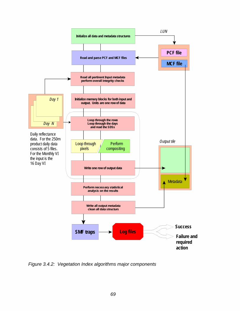
69

Initialize all data and metadata structures

Read and parse PCF and MCF files

Read all pertinent Input metadataperform overall integrity checks

Initialize memory blocks for both input and output. Units are one row of data

Loop through the rowsLoop through the days

and read the SDSs

Write one row of output data

Perform necessary statistical analysis on the results

Write all output metadataclean all data structurs

PCF file

MCF file

LUN

Day 1

Output tile

Day N

Daily reflectancedata. For the 250m product daily data consists of 5 files. For the Monthly VI the input is the 16 Day VI

Metadata

Log filesSMF trapsSuccess

Failure and required action

Loop through pixels

Perform compositing

Figure 3.4.2: Vegetation Index algorithms major components

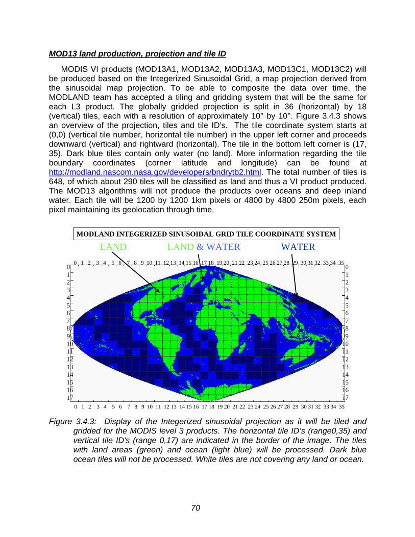
70

MOD13 land production, projection and tile ID

MODIS VI products (MOD13A1, MOD13A2, MOD13A3, MOD13C1, MOD13C2) willbe produced based on the Integerized Sinusoidal Grid, a map projection derived fromthe sinusoidal map projection. To be able to composite the data over time, theMODLAND team has accepted a tiling and gridding system that will be the same foreach L3 product. The globally gridded projection is split in 36 (horizontal) by 18(vertical) tiles, each with a resolution of approximately 10° by 10°. Figure 3.4.3 showsan overview of the projection, tiles and tile ID's. The tile coordinate system starts at(0,0) (vertical tile number, horizontal tile number) in the upper left corner and proceedsdownward (vertical) and rightward (horizontal). The tile in the bottom left corner is (17,35). Dark blue tiles contain only water (no land). More information regarding the tileboundary coordinates (corner latitude and longitude) can be found athttp://modland.nascom.nasa.gov/developers/bndrytb2.html. The total number of tiles is648, of which about 290 tiles will be classified as land and thus a VI product produced.The MOD13 algorithms will not produce the products over oceans and deep inlandwater. Each tile will be 1200 by 1200 1km pixels or 4800 by 4800 250m pixels, eachpixel maintaining its geolocation through time.

Figure 3.4.3: Display of the Integerized sinusoidal projection as it will be tiled andgridded for the MODIS level 3 products. The horizontal tile ID’s (range0,35) andvertical tile ID's (range 0,17) are indicated in the border of the image. The tileswith land areas (green) and ocean (light blue) will be processed. Dark blueocean tiles will not be processed. White tiles are not covering any land or ocean.

0 1 2 3 4 5 6 7 8 9 10 11 12 13 14 15 16 17 18 19 20 21 22 23 24 25 26 27 28 29 30 31 32 33 34 35

0 1 2 3 4 5 6 7 8 9 10 11 12 13 14 15 16 17 18 19 20 21 22 23 24 25 26 27 28 29 30 31 32 33 34 35

0123456789

1011121314151617

MODLAND INTEGERIZED SINUSOIDAL GRID TILE COORDINATE SYSTEM

LAND LAND & WATER WATER

01234567891011121314151617

71

Data flows and dependencies

Both 250m and 1km 16 day products are expected to start execution each time 16days worth of data become available for a given tile. Nonetheless, the algorithms willwait an extra 5 days in case the series data is not yet available. At the end of the 21st

day the algorithm will proceed with the currently available data series. The monthly1km algorithm will wait until all 16 day composite outputs become available (amaximum of 3 periods), it follows that the algorithm will wait an extra five days for thelast 16 day composite period of the month. All dates are to start from January 1 ofeach year, and ran into the new year if necessary, however dates are again reset toJanuary 1st.

Even though all algorithm perform thorough checking on the input data, the overallperformance and data flow is highly dependent on upstream processes, notably L2G(Level 2 Grid) and MODPRAGG (Aggregated 1km surface reflectance) as depicted byFigure 3.2.7. Currently all algorithm define a set of error-action protocols that willfacilitate troubleshooting execution problems and indicate the necessary actionsculminating in notifying our SCF which in turn will provide prompt patches if necessary.

Performance and storage load estimates

The floating point efficiency of the compositing algorithm was tested using theWalthall BRDF model for 8 and 16 day composite periods. Addition, subtraction,multiplication, and division were equally ranked as one FPO (Floating Point Operation),and comparisons, typecasts, and assignments were not recorded.

Accumulating the coefficients of the Walthall least squares matrix required 24 FPOsper data point per channel at a minimum of 5 data points and a maximum of 8 or 16.Solving explicitly for Wathall's 3 kernels using matrix inversion required a fixed cost ofapproximately 116 FPOs per channel. The total cost of a Walthall BRDF derived pixeltherefore lies between 700 and 1500 FPOs when matrix inversion is used. Incalculating only the Walthall "c" (nadir) kernel by Gaussian elimination, the fixed cost ofsolving the linear system is reduced to an estimated 30 FPOs, reducing the overallcostof a BRDF corrected pixel to between 450 and 1250 FPOs.

According to trials on global 8km AVHRR Pathfinder data, BRDF modelingcomprised approximately 18% of pixels for 8 day composites and 40% of pixels for 16day composites. The average number of data points contributing to the BRDF modeledpixels was found to be roughly 5 points for the 8 day composite and 8 points for the 16day composite. This adjusts the average number of FPOs per pixel to about 90 FPOsfor the 8 day composite and 270 FPOs for the 16 day composite as the standard case.

Given a complete tile of 4800 x 4800 land pixels, this gives an average requirementof 2.1 billion FPOs per channel per tile for 8 day composites and 6.2 billion FPOs perchannel per tile for a 16 day composite. As a worst case scenario, where the entirecomposite tile is composed of BRDF derived pixels over the entire composite period,15.3 billion FPOs are required to produce an 8 day composite tile and 28.6 billion FPOsfor 16 days.

72

The MODPR13 input and output file sizes are presented in Table 4. The storageloads of Level 2 gridded and MODPRAGG input products are given per day as well asthe total of these input files per composite periods. It should be noted that the CMGproduct input and output volumes are given for the complete globe, since they will beprocessed in a globally continuous fashion. The total global number of tiles is 648.

Table 4: Storage loads of MODIS 13 I/O products

Product names Input Sizes (MB) Output Size (MB)Level 2 Gridded (L2G) data ~1,500/dayMODPRAGG: 1km daily ~180/dayMODPR13A1: 250m/16days ~24,000 (tile) ~276 (tile)MODPR13A2: 1km/16days ~2,880 (tile) ~32 (tile)MODPR13A3: 1km/Monthly ~96 (tile) ~32 (tile)MODPR13C1: 25km/16days ~20,736 (global) ~45 (global)MODPR13C2: 25km/Monthly ~135 (global) ~33 (global)

*The actual number of global land tiles is 289

3.5 Calibration and Validation

3.5.1 Introduction

Validation of the vegetation index requires both a radiometric as well as geophysicalcomponent. Validation of VI performance in discriminating spatial and temporalvegetation differences is accomplished through independent means which includesurface biophysical measurements, theoretical canopy modeling, bioclimatic modeloutputs, and precursor airborne and satellite data sets. Post-launch validation with theMODIS sensor includes correlative measurements and emphasizes the long termperformance and quality of the VI product. The validation of the VI products are highlydependent on coupling of the VI values with ground-based "real" variations inphotosynthetic and/ or canopy structural activity.

The validation approach and measurements required are related to the scienceobjectives and planned uses of the algorithm. In this section, we outline a validationstrategy for the VI equations over a wide range of vegetation conditions. The reliability,sensitivity, limitations, assumptions, and spatial/temporal error fields associated with thealgorithm will be determined, clearly stated, as will the conditions/ situations where thealgorithm becomes weak or invalid.

Measurements and science objectives:

Spectral vegetation indices (VIs) are widely used in remote sensing as preciseradiometric measures of the spatial and temporal patterns of vegetation photosyntheticactivity, and the derivation of biophysical vegetation parameters such as leaf areaindex (LAI), fraction of absorbed photosynthetic active radiation (fPAR), net primaryproduction (NPP), biomass, and percent green cover (see Justice et al., 1985; Sellers

73

et al., 1994; Townshend et al., 1991). The ubiquitous nature of a global-based VImandates that it be robust and applicable over all biomes of the earth.

The primary science objectives of the VIs include:

• Spatial and temporal discrimination of vegetation differences (precision);

• Seasonal vegetation profiles of the growing season (phenological);

• Coupling and translation of VIs to biophysical parameters.

Thus, the vegetation indices have both radiometric and biophysical components.The VI units themselves are useful for change detection and analysis of inter- and intra-annual variability patterns in vegetation growth. The goal is to be able to detectvegetation 'changes' at such a resolution as to evaluate the impacts of both climatic andhuman processes on terrestrial systems/ processes. Derivation of biophysicalparameters is a much more sophisticated use of the vegetation index and thus requiresa more complex validation strategy. However, in both cases (radiometric andbiophysical), it needs to be made clear, that the validation of the VI algorithm concernsthe outputs, and not inputs, of the VI product. Having well calibrated and validated redand NIR reflectances does not constitute validation of the VI, as validation is concernedwith the performance of the output results, which is the ability of VI values to depictspatial/temporal variations as well as phenology and biophysical parameters.

3.5.2 Validation criteria

Validation of the VI algorithm involves testing and confirmation that the VI isperforming as designed in meeting its primary science objectives, or intended uses.Pre-launch validation efforts are aimed at testing the robustness of the algorithm withsimulation (MODIS-like) data sets. Post-launch validation efforts incorporate actualinstrument performance, product interdependence and long term performance andstability.

There are six general components to the VI validation plan:

1 Comparisons with output from canopy radiant transfer models:

These are utilized to provide a theoretical and physical basis to the VI equations toensure that the performance and behavior of the VI agrees with that of radiant transfertheory. Radiant transfer modeling is used to vary sensor specifications, vegetationstructure and amounts, canopy backgrounds, atmosphere conditions, and sun-target-view geometries. The vegetation indices are tested with simulated data sets generatedfrom simplified 2-stream models, SAIL, and Myneni 3-d canopy models. The 3-dmodels of Myneni will be conducted over six major, structurally variant, land covertypes.

2 Field-based correlative measurements:

Radiant transfer models can only give a preliminary and restrictive indication ofalgorithm performance. We are constrained to those surfaces which are readilymodeled and in which the models themselves have been validated. A more realistic

74

sampling of the spatial, radiometric, and temporal characteristics of the land surface areobtained with experimental, field measurement campaigns. Field-based radiometryenable data collection under very controlled conditions (sun, view angles, soil, etc.) withnegligible atmospheric concerns. Field-based correlative data sets will be used in bothpre- and post-launch validation activities and will involve both radiometric andbiophysical measurements over a distributed series of test sites. These generallyinvolve point-based measurements which can be coupled with intensive biophysicalmeasurements and destructive vegetation sampling.

3 Experimental aircraft data:

These are valuable in generating correlative data over larger 'footprints' or pixelsizes. These data sets are also generally accompanied with ground biophysicalmeasurements as part of larger field campaigns. AVIRIS, ASAS, AirMISR, and MASdata collected over various land cover types are particularly beneficial in validation ofthe MODIS VIs in that they allow for approximate simulation of MODIS spectralbandwidths, viewing angles, and can be degraded to MODIS pixel sizes (250 & 500 m).Airborne data sets are being amassed over major biome types and processed intosimulated MODIS VI data sets.

4 Existing satellite data sets:

These primarily include the Landsat Thematic Mapper (TM), the NOAA-AVHRR, andSeaWiFS. The Landsat TM possess the spectral bands useful in simulation nadir-based, VI imagery at 250 m and 500 m pixel sizes. The AVHRR and SeaWiFS data,with daily acquisitions, are useful in simulation and testing of the Level 3 compositingalgorithm. Landsat TM, SeaWiFS, and AVHRR data sets are being collected andprocessed over the major biome types.

Sampling requirements and tradeoffs:

As no sensor can simulate the spatial, spectral, temporal, and radiometricresolutions of the MODIS sensor, we must use, in the pre-launch phase, a limitedquantity of data derived from a suite of satellite sensors. The sampling requirementsare constrained by both the availability of global (spatial and temporal) image data setsand by the amount of biophysical ground sampling that can be accomplished.

Spatial and temporal global coverage is best accomplished with a combination ofLandsat TM, SeaWiFS, and AVHRR sampling over the major land cover types. We willuse 50-60 'test sites', in accordance with the MODIS-EOS test site program, for athorough documentation of VI spatial and temporal performance over major land covertypes. TM imagery can potentially simulate the 16-day composited MODIS- VI productsince TM is readily degraded into the 250m and 500m MODIS channels and is at near-nadir view. The daily, temporal data from the AVHRR and SeaWiFS are suited toevaluate the ability of the level 3 composited VI to construct 'growing season' andphenological curves throughout the year amidst the angular problems and distortions insuch data. Furthermore, over the major land cover types, we plan to construct LandsatTM and AVHRR/SeaWiFS growing season profiles to validate the VI compositing

75

algorithm and determine their performance and accuracy in depicting 'changes'associated with seasonal phenomena.

Measures of success:

The accuracy and performance of the VI will be assessed for each of its intendeduses/objectives. In field-measured experimental data sets, Landsat TM data, andcanopy model output, changes in biophysical parameters (LAI, fPAR, biomass, greencover) should result in corresponding changes in the VI values for a wide range ofvegetation canopies, densities, and structural conditions. The VI should be able todiscriminate differences in vegetation within and between the major land cover typesand allow for true intercomparisons of spatial and temporal vegetation variations on aglobal basis.

In the temporal domain, we are concerned with atmospheric residual contaminationand angular view angle effects on the VI compositing algorithm which may give falseindications of 'change' as well as modify the true nature of a temporal profile. In situmeasures of BRDF over some of the test sites as well as ASAS overflights at numeroussites provide for 'true' bidirectional correction of the data and an assessment as to howwell the compositing routine is minimizing angular noise. Similarly, seasonal measuresof biophysical vegetation parameters, like LAI, provide a "true" seasonal profile of avegetation growing season.

The 'continuity' role of the NDVI requires appropriate translation coefficientsbetween the AVHRR-NDVI product and the MODIS-NDVI product. These will beobtained on a regular basis over the 'test' sites via co-registration of the AVHRR andMODIS data, post-launch. In the pre-launch period, AVIRIS data are convoluted tosimulate both sensors over different land cover types.

The true measure of success of the VI product will be its performance indiscriminating spatial/temporal vegetation patterns. This will mean coupling the VIvalues with ground biophysical measures that can be independently confirmed(measured) to vary or to have changed. The VI algorithms will be evaluated with field-measured biophysical variables, including LAI, fPAR, ground cover, and structure. Wewill periodically check on a set of translation coefficients to go from VI to biophysicalparameters, over many of the land cover types.

In the case of the enhanced VI, there should also be minimal changes in VI valuesdue to canopy background differences (dry/wet soil, snow, litter, soil color, etc.) and thecapability of the EVI in removing atmospheric residual contamination (e.g., smokeplumes) will be determined with in situ data sets and sun photometer measures. Overlimited periods, the sun photometer network will be used to manually correct foratmosphere and assess the performance of the atmospheric resistance component ofthe EVI equation. The accuracy of the 'operational' atmospheric correction algorithm,based on dark object subtraction, and its impact on the VI product, will also beevaluated.

76

Examples of tests to be conducted as measures of success for the NDVI and enhancedVI include:

• Baseline test: VI values will be extracted over a global set of hyperarid sites (novegetation) for spatial and temporal (long term) invariance of the VI values.Some of these tests will be conducted jointly with MCST level 1b calibration sitesover uniform areas devoid of vegetation.

• Saturation test: VI values will be extracted over a global set of denselyforested, grassland, and agricultural sites to check and monitor the uppersensitivity range of the VIs, including 'saturation' problems.

• Threshold test: this involves a performance analysis of VI values in arid &semiarid regions to determine lower vegetation detection limits of the vegetationindices.

• Correlative measurements: biophysical measurements will be collected andmonitored (long term) over the major land cover test sites to ensure linearity andsensitivity of the VI equations over a wide range (desert to forests) of vegetationconditions.

• Seasonal profiles: detailed correlative field data and meteorological data willbe collected to assess the accuracy of the level 3 composited product indepicting growing season (phenologic) profiles for the major land cover types.

• Transition zones: gradients in climatic variation (precipitation, temperature,and topography) which are known to produce corresponding differences invegetation are ideal and will be used to test VI sensitivities.

• In-situ nadir-based reflectances: these will be measured, in conjunction withsun photometer measures, to assess the accuracy of nadir-generated outputfrom the level 3 compositing algorithm. This will include a sensitivity analysis ofthe atmospheric correction product on VI performance.

3.5.3 Pre-launch algorithm test/development activities

In the pre-launch period, a combination of sensors and data sets are used tosimulate MODIS data for the anticipated range of terrestrial surfaces with atmospheric,topographic, and angular variations. Initial validation of the VI equations themselves isaccomplished with canopy radiative transfer models such as the Myneni 6 biomecanopy code, the SAIL model, and two-stream canopy model. Field experimental datasets are also widely used including radiometric measures (e.g., PARABOLA) andaircraft sensor data. Aircraft and helicopter field measured BRDF data sets are veryvaluable in simulating MODIS view, angular relationships. Atmospheric radiativetransfer codes are also utilized to superimpose varying degrees of atmosphericcontamination onto the experimental and canopy model data sets. In this manner, thesensitivity of the VI equations to the atmosphere as well as angular variations can beassessed. Finally, precursor satellite data from the Landsat TM and AVHRR areextremely important in VI validation on a global basis. Pre-launch activities aresummarized in Table 5.

77

Table 5: Summary of pre-launch validation activities

Campaign/DataSet

Dates Sensors Purpose

Chile - GLCTS(Test Sites)

September,1996

Cimel,Exotech,(Ground andLight Aircraft)

•VI-saturation test (rainforest)•VI-baseline test (hyper-arid)•VI-threshold test (arid/semiarid)•VI-biophysical (all)

LTER Sites,U.S.A.(Long-TermEcologicalResearch)

Ongoing, 1992 -(Annual andSeasonal)

TM, AVHRR,ASAS, MAS

•VI-seasonality, compositing•Field correlative measures

- biophysical- phenologic

SCAR-B (Brasil) August toSeptember,1995

MAS, AVIRIS,Exotech,Cimel

•VI-smoke analysis•VI-saturation (bandwidths)•VI-biophysical•Continuity analysis (AVHRR,MODIS) (Tropicalforest/cerrado)

HAPEX-Sahel(Niger, Africa)

August toOctober, 1992

ASAS, TM,Exotech, Cimel

•VI-biophysical, angularcompositing threshold(Semiarid)

OTTER Transect(Oregon)

1992 ASAS, TM •VI-biophysical, angular,compositing saturation (Forests)

Monsoon '90 August toSeptember,1990September,1991Seasonal, 1992

ASAS, AVIRIS,TM, Exotech,(Air, Ground),Spectron

•VI-angular, compositingthreshold•VI-seasonality, biophysical(semiarid)

FIFE (Kansas,USA)

May toSeptember,1987 and July toAugust, 1989

ASAS, TM •VI-biophysical, angular,compositing (grassland)

BOREAS(Canada)

August toSeptember,1995

ASAS, TM •VI-biophysical, angular, smoke,compositing (boreal forest)

Global-TM/AVHRRGLCTS Pathfinder

1985 to Present TM, AVHRR •VI intercomparisons (global)•VI-compositing

MAC (MaricopaAgriculturalCenter, Arizona)

1986 to Present TM, Exotech,Sun Photometer,BRDF

•VI-seasonal; biophysical,angular•Dry-wet backgrounds

78

Some of the field experiments already incorporated into the VI validation effort include:

• SCAR-B experiment in the primary and secondary (regrowth) tropical forests ofthe Amazon. We have AVIRIS and MAS imagery for the 1995 campaign underclear and very smoky (burning season) conditions. In addition, we collectedground radiometric and biophysical data such as canopy transmittance,ceptometer readings for LAI and fPAR, and sun photometer measurements.Historical and recent values of LAI are also available from various INPEscientists for many of the sites.

• BOREAS experiment in the boreal forests of Canada. This includes MAS (1994)and AVIRIS (1996) overflights over boreal forests in the growing and snowcovered seasons. An intensive ground measurement campaign was conducted,including biophysical, and radiometric (Parabola-SE-590) measurements,including sun photometers.

• OTTER experiment in the coniferous forests of the Oregon coastal range as wellas Cascade Mountains. We have ASAS and TM data as well as LAI transectsand sun photometers.

• FIFE experiment in the tall-grass prairie, Konza Prairie, Kansas. There is ASAS,TM, and ground-based biophysical and radiometric measurements as well assun photometers.

• HAPEX-Sahel experiment in the semiarid zones of Niger, West Africa. This alsoincludes airborne (ASAS) and satellite data (TM) as well as groundmeasurements of vegetation and soil biophysical and radiometric properties, andsun photometers.

• Walnut Gulch MONSOON-90 experiment in the arid/semiarid watershed ofsoutheastern Arizona. There is ASAS and AVIRIS data, a multitemporal series ofseven Landsat TM scenes covering the 1992 growing season, and a largeamount of ground biophysical and radiometric data, including sun photometers.

• Agricultural, uniform crop canopy areas near the Konza Prairie and MaricopaAgriculture Center (MAC), Arizona. These well- controlled, precision grownbroadleaf and cereal crops represent homogeneous areas for VI validation. Theadvantage of these areas are their wide temporal and canopy structural range ofvegetation conditions ('zero' vegetation prior to planting and densely vegetatedconditions just prior to harvest). The broadleaf and cereal crops present a goodset of architectural canopy differences.

Existing satellite data:

In 1992, approximately 20 Landsat 4 & 5, TM scenes were made available to theMODIS team over some of the GLCTS candidate test sites, including broadleafdeciduous and evergreen forests, grasslands, savanna, and deserts. These TM sceneshave been processed to simulate MODIS nadir-looking imagery at 250 and 500 m pixel

79

resolutions. The data have been processed into reflectances with a new set ofcalibration (vicarious) coefficients, exo-atmosphere irradiances, and atmosphericcorrection algorithms. The atmospheric corrections include corrections based on in-situmeasurements of optical depth; and automated dark object subtraction (DOS)procedures. The derived MODIS-like reflectances are then used as input into the VIalgorithms. This data set has been useful in assessing the performance of the VIequations over a global range of vegetation conditions from sparse desert vegetation tovery dense temperate and tropical forests.

A Landsat TM multitemporal data set of seven images during the 1992 growingseason at the Walnut Gulch Experimental Watershed in southeastern Arizona has alsobeen processed into MODIS simulated VI imagery. These Landsat scenes include theU.S. - Mexican border where differences in land-use yield contrasting differences inpixel responses on both sides of the border. The data set is thus quite useful inanalyzing spatial vegetation patterns associated with land use differences and temporalphenological patterns associated with the monsoon and growing seasons. This isuseful as a threshold test in both the spatial and temporal domains.

Daily 1 km AVHRR data sets over HAPEX-Sahel, Konza Prairie, H.J. Andrews, andCoweeta sites are being initially used for development and validation of the compositingalgorithm. We plan on using daily AVHRR from other GLCTS sites as the data becomeavailable. The 8 km Pathfinder data is also useful in evaluating temporal seasonal VIprofiles over major global land cover types.

3.5.4 Post-launch activities

In the post-launch period, the primary focus will be on the validation of the globaldata product. This includes an assessment as to how the products will be evaluatedthrough the operational life of the sensor (or product). In the post-launch period,correlative measurement activities will continue over the test sites and the performanceof the algorithm over time will be carefully evaluated from which quality controls will bepresented.

Correlative measurement activities in support of VI product validation will occur overa global-based distributed network of community core test sites. Post-launch validationand the community core sites are described in the MODIS validation plan;http://modarch.gsfc.nasa.gov/MODIS/LAND/VAL/core_sites.html.

3.5.5 MQUALS

The ‘MODLAND Quick Airborne Looks’ (MQUALS) is an airborne radiometricsystem (instruments and protocol) for rapid and low cost land product validation over arange of terrestrial biome types. The package can be flown ‘below the atmosphere’ ataltitudes of 150m to 300m AGL for accurate and independent characterization ofsurface reflectances. The package can be flown at higher altitudes (500 - 1000m AGL)for scaling or large area studies. The basic package consists of calibrated andtraceable “transfer radiometers”, digital spectral cameras, an infrared thermometer and

80

a set of albedometers, all connected to a laptop computer for synchronizedmeasurements. A key feature of MQUALS is the rapid processing, “turn-around” of themeasured results to within 7 - 10 days. Through MQUALS, validation sites will becharacterized and geolocated with GPS in a consistent manner with an identical and‘traceable’ radiometric package. In conjunction with simultaneous field sampling,MQUALS will allow us to collect a self-contained set of biophysical and radiometric datafrom the same ground pixels, which can be correlated and compared with ASTER,Landsat ETM+, and MODIS/MISR pixel values.

Objectives

The main goal is to provide a 'ground truth' characterization of land cover surfacetypes to aid in EOS product validation, support linkages between radiometric accuraciesand scientific goals, and accurately tie satellite products to measurements on theground. MQUALS has the following primary objectives in support of land productvalidation:

• a land surface optical characterization, including measurement of multispectralradiances, spectral vegetation indexes, and albedo over transects up to 10 - 20kilometers,

• a consistent, well-calibrated and “traceable” instrument package, coupled to EOSvicarious calibration activities, for radiometric accuracy analysis,

• analysis of dependencies of MODIS data on sampling geometry, target scene,sun angle, and atmosphere,

• extension, correlation and scaling of ground-based vegetation biophysical (leafarea index, %cover, biomass) and radiometric (fraction of absorbedphotosynthetically active radiation) measurements to MODIS pixel sizes (250 m,500 m and 1 km),

• documentation of surface conditions and sampling of landscape variability withhigh resolution, spectral-digital camera imagery, providing qualitative and semi-quantitative checks of MODIS data.

In addition, MQUALS can provide quality assessments, uncertainty analyses, andgeneration of error bars with respect to product performance. MQUALS can alsoprovide feedback on calibrated radiance (Level 1B) processing differences and theirimpacts on land products and provide for systematic assessments of long term stabilityfor monitoring studies.

System design

The basic sensor package consists of a digital, multi-camera array, a nadir-lookingExotech radiometer with MODIS filters, two albedometers, an infrared thermometer(optional), and a laptop computer with Labview software for programmed andcoordinated data acquisition. The sensor package can be mounted on a variety ofsmall aircraft. The mounted setup is illustrated in Figure 3.5.1. The ground componentof MQUALS consists of a Spectralon reference panel with a second Exotech mountedfor continuous measurements of site irradiance.

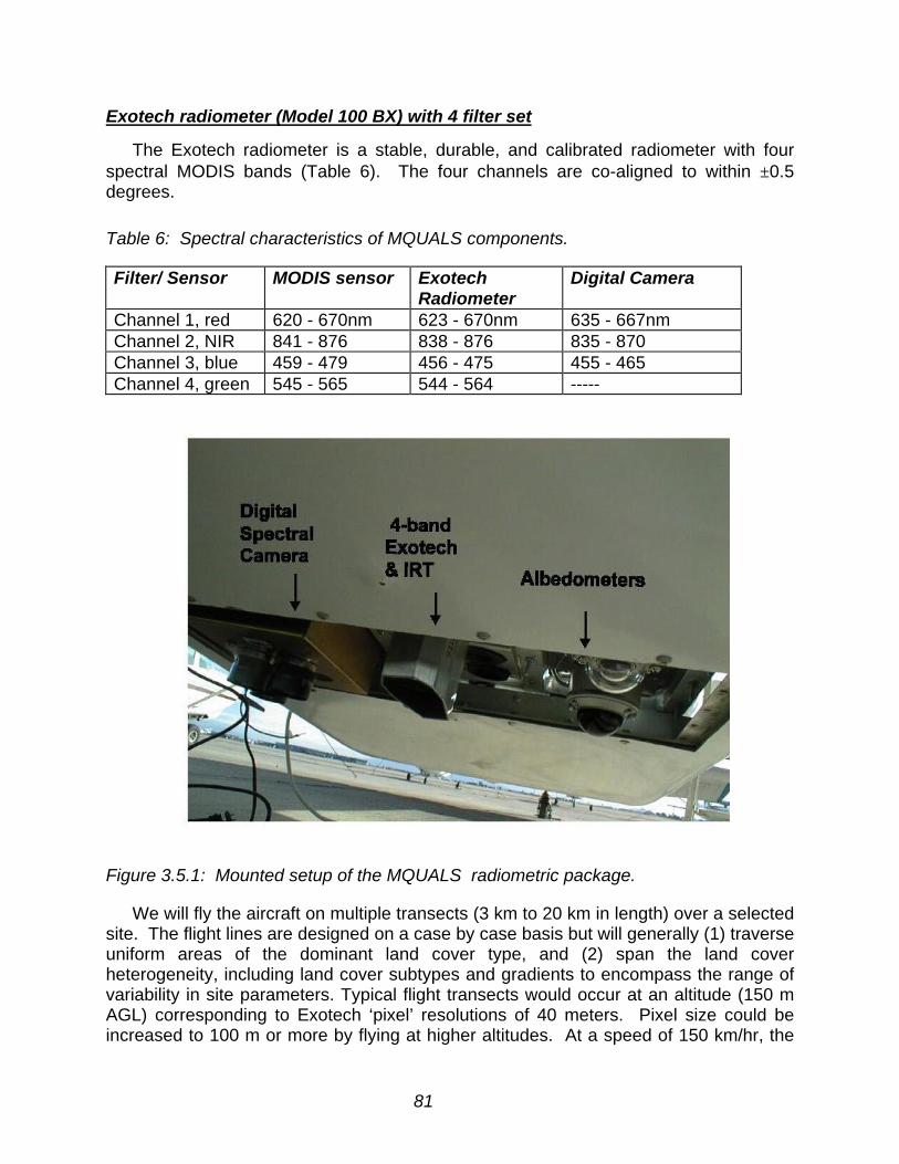
81

Exotech radiometer (Model 100 BX) with 4 filter set

The Exotech radiometer is a stable, durable, and calibrated radiometer with fourspectral MODIS bands (Table 6). The four channels are co-aligned to within ±0.5degrees.

Table 6: Spectral characteristics of MQUALS components.

Filter/ Sensor MODIS sensor ExotechRadiometer

Digital Camera

Channel 1, red 620 - 670nm 623 - 670nm 635 - 667nmChannel 2, NIR 841 - 876 838 - 876 835 - 870Channel 3, blue 459 - 479 456 - 475 455 - 465Channel 4, green 545 - 565 544 - 564 -----

Figure 3.5.1: Mounted setup of the MQUALS radiometric package.

We will fly the aircraft on multiple transects (3 km to 20 km in length) over a selectedsite. The flight lines are designed on a case by case basis but will generally (1) traverseuniform areas of the dominant land cover type, and (2) span the land coverheterogeneity, including land cover subtypes and gradients to encompass the range ofvariability in site parameters. Typical flight transects would occur at an altitude (150 mAGL) corresponding to Exotech ‘pixel’ resolutions of 40 meters. Pixel size could beincreased to 100 m or more by flying at higher altitudes. At a speed of 150 km/hr, the

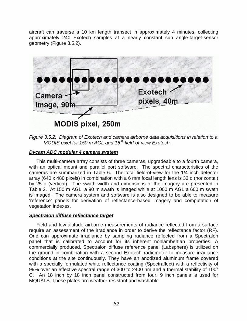
82

aircraft can traverse a 10 km length transect in approximately 4 minutes, collectingapproximately 240 Exotech samples at a nearly constant sun angle-target-sensorgeometry (Figure 3.5.2).

Figure 3.5.2: Diagram of Exotech and camera airborne data acquisitions in relation to aMODIS pixel for 150 m AGL and 15 o field-of-view Exotech.

Dycam ADC modular 4 camera system

This multi-camera array consists of three cameras, upgradeable to a fourth camera,with an optical mount and parallel port software. The spectral characteristics of thecameras are summarized in Table 6. The total field-of-view for the 1/4 inch detectorarray (640 x 480 pixels) in combination with a 6 mm focal length lens is 33 o (horizontal)by 25 o (vertical). The swath width and dimensions of the imagery are presented inTable 2. At 150 m AGL, a 90 m swath is imaged while at 1000 m AGL a 600 m swathis imaged. The camera system and software is also designed to be able to measure‘reference’ panels for derivation of reflectance-based imagery and computation ofvegetation indexes.

Spectralon diffuse reflectance target

Field and low-altitude airborne measurements of radiance reflected from a surfacerequire an assessment of the irradiance in order to derive the reflectance factor (RF).One can approximate irradiance by sampling radiance reflected from a Spectralonpanel that is calibrated to account for its inherent nonlambertian properties. Acommercially produced, Spectralon diffuse reference panel (Labsphere) is utilized onthe ground in combination with a second Exotech radiometer to measure irradianceconditions at the site continuously. They have an anodized aluminum frame coveredwith a specially formulated white reflectance coating (Spectraflect) with a reflectivity of99% over an effective spectral range of 300 to 2400 nm and a thermal stability of 100o

C. An 18 inch by 18 inch panel constructed from four, 9 inch panels is used forMQUALS. These plates are weather-resistant and washable.

83

Kipp and zonen albedometers

MQUALS will use two airborne and one ground-based pyranometers/albedometersfrom Kipp and Zonen. The clear-dome albedometer provides shortwave broadbandalbedo in the range of 305 - 2800 nm and the red dome albedometer provides NIRbroadband albedo in the range of 695 - 2800 nm. An upward looking, clear-domepyranometer is mounted on top of the airplane for irradiance measurements. Anotherset of albedometers is mounted on the ground.

Laptop computer for data logging

A Gateway 233 MHz laptop computer is used as a data logger and instrumentcontroller. Data logging frequency for all of the on-board instruments and start and stoptimes are programmed prior to the flight transects. The computer logs the data from allinstruments simultaneously. Special purpose software (LabView) is used tosynchronize these activities.

LabVIEW instrument control software with PC cards (Version 4.0)

This software is an icon-based graphical programming and data acquisition tool withfront panel user interface for control and data visualization. Complex acquisition,analysis and presentation applications can be generated in real time using a graphicalmethodology. Different data acquisition systems such as the Exotech, digital cameraand albedometers can be controlled using this software, and data acquired from theseinstruments can be checked visually for problems. PC cards, including those for signalconditioning, voltage modulation accessories, and data acquisition, are used to connectthe computer with the instruments.

GPS system (from aircraft):

Geo-positioning of the air transects is accomplished using the GPS receiver onboard the aircraft. Plans are being made to acquire a differential GPS and connect itdirectly to the laptop computer.

Calibration and traceability

The Exotech radiometers are stable and durable optical instruments that are easilycalibrated in the laboratory and can be cross-calibrated with similar instrumentationused in the field as well as on other airborne platforms. These “transfer radiometers”can also be cross-calibrated with the radiometric equipment utilized by MODISCalibration Support Team (MCST) activities, including simultaneous on-sitemeasurements at vicarious calibration field sites. The MQUALS package is currentlybeing calibrated by the Remote Sensing Group within the Optical Sciences (OSC)Department at the University of Arizona. There are three aspects to the calibration ofthe Exotech radiometers used as part of MQUALS. One aspect is to calibrateradiometers in flight using "vicarious calibration" techniques similar to those used forLandsat-5 Thematic Mapper. These methods rely heavily upon collecting ground-based data from a well-understood radiometer (an ASD FieldSpec FR in this case) withreference to a field reflectance standard (Spectralon in this case). The field referenceis calibrated in the Optical Sciences laboratory prior to the field experiment to determine

84

its bi-directional reflectance with reference to a NIST-traceable standard of reflectance.Differences in the spectral response of the Exotech radiometer relative to MODIS aretaken into account by measuring the Exotech spectral response using the OpticalSciences monochromator. An additional tool for the vicarious calibration of the Exotechradiometer, and the digital cameras as well, are a set of calibrated tarps (7 meters on aside) that are setup at the calibration sites to be viewed by the airborne camera. Thisenables characterization of the spectral response and linearity of the camera arraysystem.

A similar technique to the vicarious calibration approach is to cross-calibrate theExotech radiometer to the ground-based radiometer using the field reflectance standardto transfer the calibration from one instrument to the other. Since the ASDspectroradiometer is hyperspectral, effects due to band differences in the tworadiometers are minimized. This method can either rely on an absolute calibration ofthe ASD spectroradiometer to obtain the absolute calibration of the Exotech, or one cansimply do the cross-calibration in terms of reflectance. The latter has the advantage of"reducing" the uncertainty by not relying on the absolute calibration of one of theradiometers but a relative calibration of the reflectance standard. A similar calibrationcan be done in the lab, but the field-based approach has the advantage of using thesame spectral source that the MQUALS data set uses.

The third aspect of the MQUALS calibration is to provide a “traceable” link to theMODIS Instrument (Figure 3.5.3). This is accomplished through the use of ultrastablelaboratory radiometers that took part in a calibration round-robin to characterize theSanta Barbara Remote Sensing (SBRS) primary standard source (a large sphericalintegrating source) used in the pre-launch calibration of the MODIS instrument. Theseradiometers have also been used to calibrate the Optical Science's sources andreference panels. Thus, any instrument calibrated using Optical Science's laboratorywill have traceability to the MODIS sensor.

Note that at this point, we do not know of the radiometric stability of the multispectraldigital camera system, however we will make efforts to calibrate this instrument ifpossible. If not, this instrument will primarily be used for characterization of sceneheterogeneity and qualitative variability of component optical properties.

85

Figure 3.5.3: Diagram of the traceability of field validation measurements to the MODISinstrument.

MQUALS schedule for 1999

Testing of the MQUALS package is ongoing and has occurred mostly in the vicinityof the Semi-Arid Land-Surface-Atmosphere (SALSA) area in southeast Arizona(http://www.tucson.ars.ag.gov/salsa/salsahome.html), over a fairly uniform drygrassland. We also are testing and calibrating the system in a barren uniform areanear the Tucson International Airport. The current schedule for 1999 MQUALSdeployments is listed in the table below.

Table 7: 1999 MQUALS deployments

Site Dates Land Cover OtherRailroad Playa,NV

Late April-early May Barren, vicariouscalibration

Landsat ETM+

La Jornada,NM

Late May & September Semi-arid grass/shrub

LTER site

*Bondville , IL July - August Cropland BigFoot siteARM-CART orKonza

July - August Grassland/ agriculture PossibleMAS/AirMISRoverflight

BOREAS NSA August-September Boreal Forest BigFoot site* tentative

86

The Railroad Playa calibration experiment is expected in late April – early May ,following the April 15 launch of Landsat ETM+. In this experiment we aim to (1) crosscalibrate the MQUALS package with the MODIS vicarious calibration team; (2) registerMQUALS data with Landsat ETM+ for a homogeneous site with no vegetation; and (3)establish a zero baseline condition for vegetation indexes. The Jornada ExperimentalRange (La Jornada) near Las Cruces, New Mexico will be flown in late May (dryseason) and September (wet season) time frames. This is a semi-arid validation CoreSite with desert shrub, grassland, and mixed grass/ shrub subsites located in aprotected area which is part of the NSF’s Long Term Ecological Research (LTER) sitenetwork. The Bondville, IL and BOREAS NSA (Canada) overflights will occur inconjunction with BigFoot vegetation validation work in the July-September time frame.The objective of the BigFoot program is to provide ground validation of MODIS landcover, LAI, and FPAR, with special consideration of multiple scaling issues(http://www.fsl.orst.edu/larse/bigfoot/plan.html). The MQUALS data will provide insightfor scaling from field data to 250 m spatial resolution. Finally we would like to underflythe ER-2, with MAS/ AirMISR, over some of the ARM-CART or Konza grassland sites.

Product validation issues

We propose to characterize the optical properties of the validation sites and atvarious times of the season. These validation, ‘ground truth’ sites will be both opticallyand biophysically characterized, and atmospheric effects will be simultaneouslymeasured with sunphotometers. Precise measurements will include both theheterogeneity and uniformity of the sites and measurements will be conducted at highresolution as well as scales equivalent to that of the MODIS pixel (250 m to 1km). Wewill initially focus on the surface reflectance, vegetation indexes, albedo, LAI, FPAR andlandcover products from MODIS. MQUALS could also be useful for the snow and landsurface temperature products.

The level 3 and 4, composited products result in cloud-free maps at 16-dayintervals. These products possess a wide range of view and sun angles and ‘residual’atmospheric and cloud effects. Ground truth measurements are necessary to assesshow well the composited, as well as daily, MODIS products represent actual surfaceconditions. For example, with an independent determination of nadir-based, ‘true’surface reflectance, we can analyze where the uncertainties in the MODIS products lieand identify systematic errors. Errors associated with MODIS sensor calibration,instrument noise, atmosphere correction, BRDF correction, and the cloud maskalgorithm will propogate into the final product. However, MQUALS measurements willsimilarly be affected by calibration, bidirectional reflectance, spectral sensitivity, anddiffuse/direct irradiance effects. Thus, independent measures acquired for productvalidation will always differ somewhat from MODIS. Surface heterogeneity alsopresents difficulties in the measurement of biophysical parameters over MODIS pixelsizes. The error and lack of reproducibility in field measurements may exceed thosefrom the satellite.

We are currently drafting field validation methods and protocol documentation as aguide in the standardization of EOS field collected validation data. MQUALS flights, for

87

example, will generally be made at multiple times of the day in order to bracket a rangeof sun angles and allow for extrapolation of the radiometric data to specific solar zenithangles for standardization purposes. A single MODIS scene or composited productmay contain solar zenith angles that vary by 20°, along with sensor view angles thatvary ±55°. End-to-end validation examples involving MQUALS prior to the launch of theTerra Earth Observing satellite will be the subject of a forthcoming article. The URLaddress for MQUALS is http://gaia.fcr.arizona.edu/newmqual.html.

3.6 Exception Handling

Exceptions will be handled under three possible scenarios:

i. Tile is unavailable, incomplete, or corrupted.

ii. Tile is flagged as not usable through information contained in the metadata fields.This includes problems with tiles at high latitudes associated with low illuminationconditions. These are sometimes referred to as the terminator effect (Holben, 1986).

iii. Tile is determined not usable after unsuccessfully attempting to process it.Conditions include unfavorable atmospheric correction procedures, heavy cloud cover,missing data, unfavorable image geometry, and unusable reflectance values.

Under all three scenarios, daily products cannot be produced. No files are writtenand the output metadata is flagged appropriately. Composite products are capable offiltering the input files and only use the tiles with acceptable quality, provided there is atleast one usable day available. Otherwise, no output products are written and themetadata fields are flagged accordingly.

3.7 Error Analysis and Uncertainty Estimates

Improved predictions of global change will depend greatly on the quality and stabilityof satellite-derived time series products depicting Earth surface states and processes.As a key EOS facility instrument, the MODIS will provide a validated, high quality, 15-year data set. Error anlaysis and uncertainty estimation are vital in order to evaluatethe quality of products and algorithm performances, and to provide “reliability” estimates(confidence level) of the products as an input to the “downstream” products.

The VI error/uncertainty analyses are aimed at:

• developing a theoretical basis and set of error/uncertainty propagation equationswhich allow for modeling of the propagation and accumulation oferrors/uncertainties from all the “upstream” data processing steps into the VIproducts,

• estimating both radiometric and biophysical uncertainties of the VI products, and

• evaluating and characterizing the VI algorithm performances.

88

The resulting secondary products will include error maps over a globe and errorbudgets over the well-characterized core validation sites. Error budgets will identify themajor sources of errors for the VI products and thus allow for an overall performanceevaluation of the algorithms. These secondary products will be integrated into theQC/QA plan. The results of the analyses and uncertainty estimates will be summarizedin a living document that will be available to the user communities through the web.

The following sections describe the planned strategies for error analyses anduncertainty estimations as well as the current uncertainty estimates for several sourcesof errors.

3.7.1 Analysis approaches

The estimation of the MODIS VI uncertainties are being conducted on a step-by-step basis (e.g., Miura et al., 1999). These steps will follow the VI product generationsystem (PGS) which consists of four main steps as described in Section 2.2.10 (Figure3.7.1). Potential sources of uncertainties that may significantly impact the VI accuracieshave been identified for each level of the upstream processing steps (Figure 3.7.1).Additional sources of errors/uncertainties will be included as they are identified.

We currently utilize the “law of propagation of uncertainty” as a basis for modelingthe propagation and accumulation of uncertainties from each of potential sources intothe VI products (NCSL, 1997; Taylor and Kuyatt, 1994). We start with a functionalrelationship f that describes an estimate of a quantity of interest y, determined fromestimates of N other quantities x1, x2, … , xN :

),,,( 21 Nxxxfy K= . (15)

The law of propagation of uncertainty estimates the standard uncertainty of themeasurement result y, denoted by u(y), from the standard uncertainties of the inputestimates xi, denoted by u(xi), based on the partial derivatives of the functionalrelationship between y and xi :

∑ ∑∑∑∑−

= +=== = ∂∂

∂∂

+

∂∂

=∂∂

∂∂

=1

1 11

2

2

1 1

2 ),(2)(),()(N

i

N

ijji

ji

N

ii

i

N

i

N

jji

ji

xxux

f

x

fxu

x

fxxu

x

f

x

fyu . (16)

The uncertainty propagation equation (16) is based on a 1st-order Taylor seriesapproximation of equation 15. A set of uncertainty propagation equations designed forreflectance calibration uncertainties into atmospherically-corrected VIs are shown inAppendix F (Miura et al., 1999).

Uncertainty estimations are being and will be coupled strongly with both pre- andpost-launch validation activities. As part of the pre-launch validation activities, wecontinue to develop uncertainty propagation equations and estimate uncertainties foreach potential source of error as well as to evaluate algorithm performances.Simulated, field experimental, and the existing airborne/satellite-borne remote sensingdata (i.e., AVIRIS, ASAS, TM, SPOT, AVHRR, and SeaWiFS) are being used.

89

Assessments of the algorithm performances and accuracies have been conducted withdata sets simulated from canopy radiative transfer models (Huete and Liu, 1994),acquired during intensive field campaigns including the BOREAS (Leeuwen et al.,1996) and SCAR-B (Miura et al., 1998) experiments.

During the post-launch validation activities, the error analysis activities willspecifically focus on the evaluation of the overall product accuracies. We plan tointegrate uncertainty propagation equations for a complete estimation of total-accumulated uncertainties on a pixel-by-pixel basis and to utilize these uncertaintyestimates for the validation of the VI products. In each intensive field campaign, theuncertainty propagation equations will be applied and error budgets identifying themajor sources of errors will be produced. These uncertainty estimates for eachintensive field campaign will be summarized in a living document available to the usercommunities through the web.

The other main focus of the error analyses during the intensive field campaigns willbe on the analysis of VI-biophysical relationships followed by the biophysicaluncertainty estimations. This will be conducted over each validation site as well as on aglobal scale, which will result in the estimations of both biome-specific and globalbiophysical uncertainties of the VI products.

Error budgets will continue to be produced and updated over the core validationsites and be coupled with the long term stability monitoring as part of the QC/QA plan(see Section 3.5.2). The baseline test for the long term stability checking of the VIproducts will be also utilized to examine the validity of the uncertainty propagationequations and estimated uncertainties.

90

Figure 3.7.1: “End-to-end” analysis approaches of the VI error/uncertainties. Potentialsources of errors and uncertainties considered in each upstream processing stepare also listed.

91

3.7.2 Uncertainty estimates

Among many potential sources of error and uncertainties, we have so far evaluatedthe VI product accuracies due to 1) reflectance calibration uncertainty, 2) spectral bandshift, and 3) band-to-band coregistration error. The following summarizes the results ofthese analyses.

Reflectance calibration uncertainty

The radiometric calibration of the AVHRR sensors has been one of the mostintensively studied problems. Numerous studies have shown that the calibration of theAVHRR instrument has changed substantially following launch and drifted subsequentlyover time, which in turn creates interannual variability in NDVI assessments unrelatedto global vegetation dynamics (Frouin and Gautier, 1987; Holben et al., 1990; Che andPrice, 1992; Kaufman and Holben, 1993; Rao 1993; Teillet et al., 1990). As a key EOSinstrument, the MODIS has placed a strong emphasis on its calibration algorithm. Itsthree on-board calibrators for the calibration of the solar reflective regions willaccomplish a higher precision in calibration results and will be periodically validatedthrough vicarious calibration techniques for detection and correction of drift incalibration gains over time (Barbieri et al., 1997).

Miura et al. (1999) and Huete and Liu (1994) evaluated the impact of reflectancecalibration uncertainties on the accuracies of the VI product using the experimental dataset (Huete et al., 1985) with the 6S radiative transfer code (Vermote et al., 1997a) foratmosphere simulations. Miura et al. (1999) developed an approach to modelpropagation of uncertainties from calibrated top-of-atmosphere (TOA) reflectances toatmospherically-corrected VIs (Appendix F).

The resultant VI uncertainties ucal(VI) varied with both surface reflectances andatmospheric conditions (Miura et al., 1999). The largest uncertainties of the NDVI andARVI were observed for dark targets with little or no vegetation (Figure 3.7.2a,c). TheSAVI uncertainties were nearly constant throughout a range of target brightness andvegetation abundance (Figure 3.7.2b). The EVI uncertainties linearly increased withincreasing EVI values (Figure 3.7.2d). Atmosphere turbidities increased calibrationuncertainties in all the VIs through its effect on TOA reflectances. The VI uncertaintieswere also found to decrease when the calibration errors were positively correlatedbetween bands.

The mean VI uncertainties were estimated to be +/- 0.01 VI units for the NDVI andSAVI, and +/- 0.02 VI units for the ARVI and EVI under normal atmosphere conditions(>= 20 km visibility) and a 2% reflectance calibration uncertainty (Miura et al., 1999).The higher uncertainties in the ARVI and EVI resulted from the inclusion of the blueband, adding to the overall calibration uncertainty budget.

Their sensitivity analyses showed that the VI uncertainties increased linearly withincreases in reflectance calibration uncertainties for all the VIs examined in their study,from which the required calibration uncertainties to attain a desired VI accuracy wereobtained (Table 8).

92

Figure 3.7.2: Uncertainties of the a) NDVI, b) SAVI, c) ARVI, and d) EVI due to a 2%reflectance calibration uncertainty, ucal(VI), propagated through a turbidatmosphere (continental aerosols with a 10 km visibility). The band calibrationerrors were treated as uncorrelated. The figure includes ucal(VI) for dark(Cloverspring) and bright (Superstition) backgrounds.

Table 8: Predicted Reflectance Calibration Uncertainties (%) Requirements for DesiredLevels of VI Uncertainty

Required Reflectance Calibration Uncertainties (%)ucal(VI) Desired NDVI SAVI ARVI EVI

0.01 1.9% 2.1% 1.0% 1.2%0.02 3.8% 4.2% 1.9% 2.4%0.05 9.4% 10.5% 4.8% 5.9%0.10 18.9% 21.1% 9.6% 11.9%

93

Spectral band shift and band-to-band coregistration error

In addition to the calibration uncertainty, the MODIS L1B product will include thespectral band shift information in the solar reflective bands and the coregistrationaccuracy of other bands relative to the reference band per granule basis (Barbieri et al.,1997).

Huete and Liu (1994) assessed expected errors of the VIs due to a 2 nm centerwavelength shift and a 20% band-to-band coregistration error. A SAIL model simulation(Verhoef, 1984) was performed using a single-layer one-component canopy model witha uniform leaf angle distribution. The reflectance and transmittance properties of cedartree leaves were used with canopy LAI values from 0.0 to 3.0 for a solar zenith angle of40 O and nadir view.

All of the VIs examined in the study (the NDVI, SAVI, ARVI, and EVI) have an errorof +/- 0.01 VI unit due to a 2 nm center wavelength shift. For the band-to-bandcoregistration error, the NDVI and EVI have an error of +/- 0.01 VI unit while the SAVIand ARVI have an error of +/- 0.03. The results are summarized in Table 9.

Table 9: Expected VI Error due to the Spectral Band Shift and Band-to-bandCoregistration Error (in VI unit)

NDVI SAVI ARVI EVI

Band Shift 0.01 0.01 0.01 0.01Coregistration 0.01 0.03 0.03 0.01

4 Constraints, Limitations, and Assumptions

Only day time, cloud free data should be processed to produce the VI. We assumethat the data is cloud-free and that sub-pixel clouds will be filtered with a compositingcycle. We are assuming fairly good geolocation and registration of multi-temporal data(within MODIS specifications) and we will need a careful assessment of geometricperformance post-launch. We are assuming that a first order topographic correction willbe made post-launch in the derivation of surface reflectances. We envisage that 16days of data will be stored and kept on-line in order to look for anomalies.

94

REFERENCES

Ackerman, S., Strabala, K., Menzel, P., Frey, R., Moeller, C., Gumley, L., Baum, B.,Schaaf, C., Riggs, G., and Welch, R. (1996), Discriminating Clear-sky fromCloud with MODIS Algorithm Theoretical Basis Document V3,http://eospso.gsfc.nasa.gov/atbd/modistables.html.

Agbu, P. A. and James, M. E. (1994), The NOAA/NASA Pathfinder AVHRR Land DataSet User’s Manual. Goddard Distributed Active Archive Center, NASA, GoddardSpace Flight Center, Greenbelt, MD.

Archard, F., Malingreau, J. P., Phulpin, T., Saint, G., Saugier, B., Seguin, B., and VidalMadjar, D. (1994), A mission for global monitoring of the continental biosphere.VEGETATION International Users Committee Secretariat, Joint ResearchCentre, Institute for Remote Sensing Applications, I-21020 ISPRA (Va) Italy.http://www-vegetation.cst.cnes.fr:8050/.

Asrar, G., Fuchs, M., Kanemasu, E. T., and Hatfield, J. L. (1984), Estimating absorbedphotosynthetic radiation and leaf area index from spectral reflectance in wheat,Agron. J., 76:300-306.

Asrar, G., Myneni, R. B., and Choudhury, B. J. (1992), Spatial heterogeneity invegetation canopies and remote sensing of absorbed photosynthetically activeradiation: a modeling study, Remote Sens. Environ., 41:85-101.

Barbieri, R., Montgomery, H., Qiu, S., Barnes, B., Knowles, D., Jr., Che, N., andGoldberg, I. L. (1997), The MODIS Level 1B Algorithm Theoretical BasisDocument Version 2.0 (ATBMOD-01), NASA Goddard Space Flight Center,Greenbelt, Maryland 20771, USA, 68p.

Baret, F. and Guyot, G. (1991), Potentials and limits of vegetation indices for LAI andAPAR assessment, Remote Sens. Environ., 35:161-173.

Baret, F., Guyot, G., and Major, D. (1989), TSAVI: a vegetation index which minimizessoil brightness effects on LAI and APAR estimation, in 12th Canadian Symp. onRemote Sensing and IGARSS’90, Vancouver Canada, 10-14 July 1989.

Barker, J. L., Brown, K. S., and Harnden, J. M. K. (1993), MODIS: Calibration &Characterization Algorithm Theoretical Basis Document (Cal ATBD), Version 0, 1July, 1993.

Bartlett, D. S., Hardisky, M. A., Johnson, R. W., Gross, M. F., Klemas, V., and Hartman,J. M. (1988), Continental scale variability in vegetation reflectance and itsrelationship to canopy morphology, Int. J. Remote Sens., 9:1223-1241.

Bausch, W. (1993), Soil background effects on reflectance-based crop coefficients forcorn, Remote Sens. Environ, 46:1-10.

Begue, A. (1993), Leaf area index, intercepted photosynthetically active radiation, andspectral vegetation indices: a sensitivity analysis for regular-clumped canopies,Remote Sens. Environ., 46:45-59.

95

Buschmann, C., and Nagel, E. (1993), In vivo spectroscopy and internal optics ofleaves as basis for remote sensing of vegetation, Int. J. Remote Sens., 14:711-722.

Che, N. and Price, J. C. (1992), Survey of radiometric calibration results and methodsfor visible and near infrared channels of NOAA-7, -9, and -11 AVHRRs, RemoteSens. Environ., 41:19-27.

Choudhury, B. J. (1987), Relationships between vegetation indices, radiationabsorption, and net photosynthesis evaluated by a sensitivity analysis, RemoteSens. Environ., 22:209-233.

Cihlar, J., Manak, D., and D’Iorio, M. (1994a), Evaluation of Compositing Algorithms forAVHRR Data over Land, IEEE Trans. Geosc. Remote Sens., 32:427-437.

Cihlar, J., Manak, D., and Voisin, N. (1994b), AVHRR bidirectional reflectance effectsand compositing, Remote Sens. Environ., 48:77-88.

Cihlar, J. C., Ly, H., Li, Z., Chen, J., Pokrant, H., and Huang, F. (1997), Multi temporal,multichannel AVHRR data sets for land biosphere studies—Artifacts andcorrections, Remote Sens. Environ., 60:35-57.

Clevers, J. G. P. W. (1989), The application of a weighted infrared-red vegetation indexfor estimating leaf area index by correcting soil moisture, Remote Sens. Environ.,29:25-37.

Clevers, J. G. P. W. and Verhoef, W. (1993), LAI estimation by means of the WDVI: asensitivity analysis with a combined PROSPECT-SAIL model, Remote Sens.Rev., 7:43-64.

Colwell, J. E. (1974), Vegetation canopy reflectance, Remote Sens. Environ., 3:175-183.

Cooper, K., Smith, J. A., and Pitts, D. (1982), Reflectance of a vegetation canopy usingthe adding method, Appl. Opt., 21: 4112-19.

Curran, P. J. (1980), Relative reflectance data from preprocessed multispectralphotography, Int. J. Remote Sens., 1:77-83.

Curran, P. J. (1982), Multispectral remote sensing for estimating biomass andproductivity, in Plants and the Daylight Spectrum, edited by H. Smith, LondonAcademic Press.

Daughtry, C. S. T., Gallo, K. P., Goward, S. N., Prince, S. D., and Kustas, W. P. (1992),Spectral estimates of absorbed radiation and phytomass production in corn andsoybean canopies, Remote Sens. Environ, 39:141-152.

Deering, D. W. and Leone (1986), A sphere-scanning radiometer for rapid directionalmeasurements of sky and ground radiance, Remote Sens. Environ., 19:1-24.

Deering, D. W. (1978), Rangeland reflectance characteristics measured by aircraft andspacecraft sensors. Ph.D. Dissertation, Texas A & M University, College Station,TX, 338 pp.

96

Demetriades-Shah, T. H., Steven, M. D., and Clark, J. A. (1990), High resolutionderivative spectra in remote sensing, Remote Sens. Environ., 33:55-64.

Eidenshink, J. C. and Faundeen, J. L. (1994), The 1km AVHRR global land data set:first stages in implementation, Int. J. Remote Sensing, 15(17):3443-3462.

Elvidge, C. D. and Chen, Z. (1995), Comparison of broad-band and narrow-band redand near-infrared vegetation indices, Remote Sens. Environ., 54:38-48.

Flittner, D. E. and Slater, P. N. (1991), Stability of narrow-band filter radiometers solar-reflective range, Photogramm. Eng. Remote Sens., 57:165-171.

Franklin, J. F., Bledsoe, C. S., and Callahan, J. T. (1990), Contributions of the long-term ecological research program, BioScience, 40:509-523.

Fraser, R. S. and Kaufman, Y. J. (1985), The relative importance of aerosol scatteringand absorption in remote sensing, IEEE Trans. Geosci. Remote Sens., 23: 625-633.

Frouin, R. and Gautier, C. (1987), Calibration of NOAA-7 AVHRR, GOES-5, andGOES-6 VISSR/VAS solar channels, Remote Sens. Enviorn., 22:73-101.

Fung, Y., Tucker, C. J. and Prentice, K. C. (1987), Application of Advanced Very HighResolution Radiometer vegetation index to study atmosphere-biosphereexchange of CO2, J. Geoph. Res., 92, 2999-3015.

Gallo, K. P., Daughtry, C. S. T., and Bauer, M. E. (1985), Spectral estimation ofabsorbed photosynthetically active radiation in corn canopies, Remote Sens.Environ., 17:221-232.

Gitelson, A. A., Kaufman, Y. J., and Merzlyak (1997), An atmospherically resistant“green” vegetation index (ARGI) for EOS-MODIS, Remote Sens. Environ.,58:289-298.

Goel, N. S. (1988), Models of vegetation canopy reflectance and their use in estimationof biophysical parameters from reflectance data, Remote Sens. Rev., 4: 1-222.

Goward, D. G., Turner, S., Dye, D. G., and Liang, J. (1994), University of Marylandimproved Global Vegetation Index, Int. J. Remote Sensing, 15(17):3365-3395.

Goward, S. N., Markham, B. L., Dye, D. G., Dulaney, W., and Yang, J. (1991),Normalized difference vegetation index measurements from the Advanced VeryHigh Resolution Radiometer, Remote Sens. Environ., 35:257-277.

Goward, S. N. and Huemmrich, K. F. (1992), Vegetation canopy PAR absorptance andthe normalized difference vegetation index: an assessment using the SAILmodel, Remote Sens. Environ., 39:119-140.

Goward, S. N., Markham, B., Dye, D. G., Dulaney, W., and Yang, J. (1991), Normalizeddifference vegetation index measurements from the Advanced Very HighResolution Radiometer, Remote Sens. Environ., 35:257-277.

Goward, S. N., Tucker, C. J., and Dye, D. G. (1985), North American vegetationpatterns observed with the NOAA-7 advanced very high resolution radiometer,Vegetatio, 64:3-14.

97

Graetz, D. (1990), Romote sensing of terrestrial ecosystem structure: an ecologist'spragmatic view, In Remote Sensing of Biosphere Functioning; Ch. 2.,pp 5-30.Springer Verlag, N.Y., 312pp.

Gutman, G. (1991), Vegetation indices from AVHRR: an update and future prospects,Remote Sens. Environ., 35:121-136.

Hall, F. G., Huemmrich, K. F., and Goward, S. N. (1990), Use of narrow-band spectra toestimate the fraction of absorbed photosynthetically active radiation, RemoteSens. Environ., 32:47-54.

Heilmen, J. L. and Kress, M. R. (1987), Effects of vegetation on spectral irradiance atthe soil surfaces, Agron. J., 79:765-768.

Holben, B. N., Kaufman, Y. J., and Kendall, J. D. (1990), NOAA-11 AVHRR visible andnear-IR inflight calibration, Int. J. Remote Sens., 11(8):1511-1519.

Holben, B. N. (1986), Characterization of maximum value composites from temporalAVHRR data, Int. J. Remote Sensing, 7:1417-1434.

Hooker, S. B., Esaias, W. E., Feldman, G. C., Gregg, W. W., and McClain, C. R.(1992), An Overview of SeaWiFS and Ocean Color. NASA Tech. Memo.104566, Vol. 1, S.B. Hooker and E.R. Firestone, Eds., NASA Goddard SpaceFlight Center, Greenbelt, Maryland, 24 pp.

Huete, A. R. (1988), A soil adjusted vegetation index (SAVI), Remote Sens. Environ.,25:295-309.

Huete, A. R. and Liu, H. Q. (1994), An error and sensitivity analysis of the atmospheric-and soil-correcting variants of the NDVI for the MODIS-EOS, IEEE Tans. Geosci.Remote Sens., 32(4):897-905.

Huete, A., Justice, C. and Liu, H. (1994), Development of vegetation and soil indices forMODIS-EOS, Remote Sens. Environ., 49:224-234.

Huete, A. R. and Tucker, C. J. (1991), Investigation of soil influences in AVHRR redand near-infrared vegetation index imagery, Int. J. Remote Sensing, 12:1223-1242.

Huete, A. R. and Warrick, A. W. (1990), Assessment of vegetation and soil waterregimes in partial canopies with optical remotely sensed data, Remote Sens.Environ., 32:155-167.

Huete, A. R., Hua, G., Qi, J., Chehbouni, A., and van Leeuwen, W.J.D.G. (1992),Normalization of multidirectional red and NIR reflectances with the SAVI, RemoteSens. Environ., 40:1-20.

Huete, A. R., Jackson, R. D., and Post, D. F. (1985), Spectral response of a plantcanopy with different soil backgrounds, Remote Sens. Environ., 17:37-53.

Huete, A. R., Liu, H. Q., Batchily, K., and van Leeuwen, W. (1997), A comparison ofvegetation indices over a global set of TM images for EOS-MODIS, RemoteSens. Environ., 59:440-451.

98

Hutchinson, C. F. (1991), Use of satellite data for Famine Early Warning in sub-Saharian Africa, Int. J. Remote Sensing, 12(6):1405-1421.

IGBP (1992), The International Geosphere-Biosphere Programme: A Study of GlobalChange, Improved Global Data for Land Applications, IGBP Report No. 20,Stockholm, Sweden: IGBP Secretariat.

Irons, J. R., Ranson, K. J., Williams, D. L., Irish, R. R., and Huegel, F. G. (1991), An off-nadir imaging spectroradiometer for terrestrial ecosystem studies, IEEE Trans.Geosci. and Remote Sens., 29:66-74.

Jackson, R. D. and Huete, A. R. (1991), Interpreting vegetation indices, Prev. Vet.Med., 11:185-200.

Jackson, R. D. and Pinter, Jr., P. J. (1986), Spectral response of architecturally differentwheat canopies, Remote Sens. Environ., 20:43-56.

Jacquemoud, S. and Baret, F. (1990), PROSPECT: A model of leaf optical propertiesspectra, Remote Sense. Environ., 3: 43-47.

James, M. D. and Kalluri, S. N. V. (1994), The Pathfinder AVHRR land data set: Animproved coarse resolution data set for terrestrial monitoring, Int. J. RemoteSensing, 15(17):3347-3363.

Jordan, C. F. (1969), Derivation of leaf area index from quality of light on the forestfloor, Ecology, 50:663-666.

Justice, C., Hall, D., Salomonson, V., Privette, J., Riggs, G., Strahler, A., Lucht, W.,Myneni, R.,Knjazihhin, Y., Running, S., Nemani, R., Vermote, E., Townshend, J.,Defries, R., Roy, D., Wan, Z.,Huete, A., van Leeuwen, W., Wolfe, R., Giglio, L.,Muller, J-P., Lewis, P., and Barnsley, M. (1998), The Moderate ResolutionImaging Spectroradiometer (MODIS): Land remote sensing for global changeresearch, IEEE Trans. Geosci. and Remote Sens., 36(4):1228-1249.

Justice, C. O., Townshend, J. R. G., Holben, B. N., and Tucker, C. J. (1985), Analysisof the phenology of global vegetation using meteorological satellite data, Int. J.Remote Sensing, 6:1271-1318.

Kaufman, Y. J. (1989), The atmospheric effect on remote sensing and its corrections, inTheory and Applications of Optical Remote Sensing (G. Asrar, Ed.), John Wiley& Sons Inc., New York, pp. 336-428.

Kaufman, Y. J. and Holben, B. N. (1993), Calibration of the AVHRR visible and near-IRbands by atmospheric scattering, ocean glint and desert reflection, Int. J.Remote Sensing, 14(1):21-52.

Kaufman, Y. J. and Tanre, D. (1992), Atmospherically resistant vegetation index (ARVI)for EOS-MODIS, IEEE Trans. Geosci. Remote Sensing, 30:261-270.

Kaufman, Y. J. and Tanre, D. (1996), Strategy for direct and indirect methods forcorrecting the aerosol effect on remote sensing: from AVHRR to EOS-MODIS,Remote Sens. Environ., 55:65-79.

99

Kimes, D. S., Holben, B. N., Tucker, C. J., and Newcomb, W. W. (1984), Optimaldirectional view angles for remote-sensing missions, Int. J. Remote Sensing,5(6):887-908.

Kimes, D. S., Newcomb, W. W., Tucker, C. J., Zonneveld, I. S., Van Wijngaarden, W.,De Leeuw, J., and Epema, G. F. (1985), Directional reflectance factor distributionfor cover types of Northern Africa, Remote Sens. Environ., 18:1-19.

King, M. D., Kaufman, Y. J., Menzel, W. P., and Tanre, D. (1992), Remote sensing ofcloud, aerosol, and water vapor properties from the Moderate ResolutionImaging Spectrometer (MODIS), IEEE Trans. Geosci. Remote Sensing, 30:2-27.

Kneizys, F. X., Shettle, E. P., Abreu, L. W., Chetwynd, J. H., Anderson, G. P., Gallery,W. O., Selby, J. E. A., and Clough, S. A. (1988), Users Guide to LOWTRAN 7,Report AFGL-TR-88-0177, AFRCL, Bedford, Mass., August, 137 pp.

Kuchler, A. W. (1995), Natural vegetation map, In: Rand McNally Goode’s World Atlas;19th edition. Eds. Espenshade E.B. Hudson, J.C., Morrison, J.L., p 18-19.

Leeuwen van, W. J. D., Huete, A. R., and Laing, T. W. (1999), MODIS vegetation indexcompositing approach: A prototype with AVHRR data, Remote Sens. Environ.(accepted).

Leeuwen van, W. J. D., Huete, A. R., Jia, S., and Walthall, C. L. (1996), Comparison ofvegetation index compositing scenarios: BRDF versus maximum VI approaches,IEEE-IGARSS ’96, Lincoln, Nebraska, 3:1423-1425.

Leeuwen van, W. J. D., Huete, A. R., Duncan, J., and Franklin, J. (1994), Radiativetransfer in shrub savanna sites in Niger -- preliminary results from HAPEX-II-Sahel: 3. Optical dynamics and vegetation index sensitivity to biomass and plantcover, Agricultural and Forest Meteorology, 69:267-288.

Leeuwen van, W. J. D., Huete, A. R., Didan, K., and Laing, T. (1997a), Modeling bi-directional reflectance factors for different land cover types and surfacecomponents to standardize vegetation indices, In Proceedings of the 7th Int.Symposium on Physical Measurements and Signatures in Remote Sensing,Courcheval, France; 7-11April 1997. pp 373-380.

Leeuwen van, W. J. D., Huete, A. R., and Laing, T. (1998), Evaluation of the MODISvegetation index compositing algorithm using SeaWiFS data, IEEE- IGARSS'98,Seattle.

Leeuwen van, W. J. D., Laing, T. W., and Huete, A. R. (1997b), Quality assurance ofglobal vegetation index compositing algorithms using AVHRR Data, IEEE-IGARSS'97, Singapore, pp 341-343.

Liu, H. Q., and Huete, A. R. (1995), A feedback based modification of the NDVI tominimize canopy background and atmospheric noise, IEEE Trans. Geosci.Remote Sensing, 33:457-465.

Lucht, W. (1998), Expected retrieval accuracies of bidirectional reflectance and albedofrom EOS-MODIS and MISR angular sampling, J. Geoph. Res., 103(D8):8763-8778.

100

Major, D. J., Baret, F., and Guyot, G. (1990), A ratio vegetation index adjusted for soilbrightness, Int. J. Remote Sensing, 11:727-740.

Meyer, D., Verstraete, M., and Pinty, B. (1995), The effect of surface anisotropy andviewing geometry on the estimation of NDVI from AVHRR, Remote Sens. Rev.,12:3-27.

Middleton, E. M. (1991), Solar zenith angle effects on vegetation indices in tallgrassprairie, Remote Sens. Environ., 38:45-62.

Miura, T., Huete, A. R., van Leeuwen, W. J. D., and Didan, K. (1998), Vegetationdetection through smoke-filled AVIRIS images: An assessment using MODISband passes, J. Geophys. Res., 103(D24):32,001-32,011.

Miura, T., Huete, A. R., and Yoshioka, H. (1999), Evaluation of sensor calibrationuncertainties on vegetation indices for MODIS (submitted to IEEE Tans. Geosci.Remote Sens.).

Moody, A. and Strahler, A. H. (1994), Characteristics of composited AVHRR data andproblems in their classification, Int. J. Remote Sensing, 15(17):3473-3491.

Morisette, J. T., Privette, J. L., Justice, C. O., and Running, S. W. (1998), MODIS LandValidation Plan; MODIS Land Discipline Team,http://modarch.gsfc.nasa.gov/MODIS/LAND/VAL/land_val_plan.pdf

Myneni, R. B. and Asrar, G. (1993), Atmospheric effects and spectral vegetationindices, Remote Sens. Environ, 390-402.

Myneni, R. B., Hall, F. G., Sellers, P. J., and Marshak, A. L. (1995), The interpretationof spectral vegetation indices, IEEE Trans. Geosci. Remote Sensing, 33(2):481-486.

Myneni, R. B, Keeling, C. D., Tucker, C. J., Asrar, G., and Nemani, R. R. (1997),Increased plant growth in the northern high latitudes from 1981 to 1991, Nature386:698-702.

Nakajima, T. Y., Nakajima, T., Nakajima, M., Fukushima, H., Kuji, M., Uchiyama, A.,and Kishino, M. (1998), Optimization of the Advanced Observing Satellite GlobalImager channels by use of radiative transfer calculations, Applied Optics,37(15):3149-3163.

NCSL (1997), American National Standard for Expressing Uncertainty – U.S. Guide tothe Expression of Uncertainty in Measurement, ANSI/NCSL Z540-2-1997,National Conference of Standards Laboratories (NCSL), Boulder, CO, 101p.

Perry, C. R., Jr. and Lautenschlager, L. F. (1984), Functional equivalence of spectralvegetation indices, Remote Sens. Environ., 14:169-182.

Pinter, P. J., Jr. (1993), Solar angle independence in the relationship between absorbedPAR and remotely sensed data for alfalfa, Remote Sens. Environ, 46:19-25.

Pinty, B. and Verstaete, M. M. (1992), GEMI: A non-linear index to monitor globalvegetation from satellites, Vegetatio, 101:15-20.

101

Price, J. C. (1987), Calibration of satellite radiometers and the comparison of vegetationindices, Remote Sens. Environ., 21:419-422.

Price, J. C. (1992), Estimating vegetation amounts from visible and near infraredreflectance measurements, Remote Sens. Environ., 41:29-34.

Prince, S. D. and Justice, C. O. (1991), (Editorial) Special issue on coarse resolutionremote sensing of the Sahelian environment, Int. J. Remote Sensing,12(6):1137-1146.

Prince, S. D. (1991), A model of regional primary production for use with coarseresolution satellite data, Int. J. Remote Sensing, 12(6):1313-1330.

Prince, S. D., Justice, C. O., and Moore, B. (1994), Remote Sensing of NPP, IGBP DISWorking Paper #10, IGBP-DIS, Paris.

Prince, S. D., Kerr, Y. H., Goutorbe, J. P., Lebel, T., Tinga, A., Bessemoulin, P.,Brouwer, J., Dolman, A. J., Engman, E. T., Gash, J. H. C., Hoepffner, M., Kabat,P., Monteny, B., Said, F., Sellers, P., and Wallace, J. (1995), Geographical,biological and remote sensing aspects of the Hydrologic Atmospheric PilotExperiment in the Sahel (HAPEX-Sahel), Remote Sens. Environ., 51:215-234.

Privette, J. L., Eck, T. F., and Deering, D. W. (1997), Estimating spectral albedo andnadir reflectance through inversion of simple BRDF models withAVHRR/MODIS-like data, J. Geophys. Res., 102(D24):29,529-29,542.

Privette, J. L., Myneni, R. B., Emery, W. J., and Hall, F. G. (1996), Optimal samplingconditions for estimating grassland parameters via reflectance model inversions,IEEE Trans. Geosci. Remote Sens., 34(1):272-284.

Qi, J. and Kerr, Y. (1997), On current compositing algorithms, Remote Sens. Rev.,15:235-256.

Qi, J., Chehbouni, A., Huete, A. R., Kerr, Y. H., and Sorooshian, S. (1994), A modifiedsoil adjusted vegetation index, Remote Sens. Environ, 48:119-126.

Qi, J., Huete, A. R., Hood, J., and Kerr, Y. (1994), Compositing multi-temporal remotesensing data sets, PECORA 11, Symposium on land information systems, SiouxFalls August 1993, p.206-213.

Qi, J., Huete, A. R., Moran, M. S., Chehbouni, A., and Jackson, R. D. (1993a),Interpretation of vegetation indices derived from multi-temporal SPOT images,Remote Sens. Environ., 44:89-101.

Rahman, H., Pinty, B., and Verstraete, M. M. (1993), Coupled surface-atmospherereflectance (CSAR) model 2. Semiemperical surface model usable with NOAAAVHRR, J. Geophys. Res., 89(D11):20,791-20,801.

Raich, J. W. and Schlesinger, W. H. (1992), The global carbon dioxide flux in soilrespiration and its relationship to vegetation and climate, Tellus, 44B:81-99.

Rao, C. R. N., Ed. (1993), Degradation of the visible and near-infrared channels of theAdvanced Very High Resolution Radiometer on the NOAA-9 spacecraft:assessment and recommendations for corrections, NOAA Technical Report

102

NESDIS 70, Dept. of Commerce, NOAA, National Environmental Satellite, Data,And Information Service, 25p.

Richardson, A. J. and Wiegand, C. L. (1977), Distinguishing vegetation from soilbackground information, Photogramm. Eng. Remote Sens., 43:1541-1552.

Roujean, J. L., Leroy, M., Podaire, A., and Deschamps, P. Y. (1992), Evidence ofsurface reflectance bidirectional effects from a NOAA/AVHRR multi-temporaldata set, Int. J. Remote Sensing, 13(4), 685-698.

Roy, D. P. (1997), Investigation of the maximum normalized difference vegetation index(NDVI) and the maximum surface temperature (Ts) AVHRR compositingprocedures for the extraction of NDVI and Ts over forest, Int. J. Remote Sens.,18(11):2383-2401.

Running, S. W. (1990), Estimating terrestrial primary productivity by combining remotesensing and ecosystem simulation, In Ecological Studies Vol “Remote Sensingof Biosphere Functioning”, H. Mooney and R. Hobbs., eds., Springer-Verlag,pp.65-86.

Running, S. W. and Nemani, R. R. (1988), Relating seasonal patterns of the AVHRRvegetation index to simulated photosynthesis and transpiration of forest indifferent climates, Remote Sens. Environ., 24:347-367.

Running, S. W., Justice, C. O., Salomonson, V., Hall, D., Barker, J., Kaufman, Y. J.,Strahler, A. H., Huete, A. R., Muller, J. P., Vanderbilt, V., Wan, Z. M., Teillet, P.,and Carneggie, D. (1994), Terrestrial remote sensing science and algorithmsplanned for EOS/MODIS, Int. J. Remote Sensing, 17:3587-3620.

Running, S. W., Nemani, R. R., Peterson, D. L., Band, L. E., Potts, D. F., Pierce, L. L.,and Spanner, M. A. (1989), Mapping regional forest evapotranspiration andphotosynthesis by coupling satellite data with ecosystem simulation, Ecology,70:1090-1101.

Runyon, J., Waring, R. H., Goward, S. N., and Welles, J. M. (1994), Environmentallimits on net primary production and light-use efficiency across the Oregontransect, Ecological Applications, 4:226-237.

Salomonson, V. V., Barnes, W. L., Maymon, P. W., Montgomery, H. E., and Ostrow, H.(1989), MODIS: advanced facility instrument for studies of the earth as a system,IEEE Trans. Geosci. Remote Sens., 27:145-153.

Sellers, P. J. (1985), Canopy reflectance, photosynthesis and transpiration, Int. J.Remote Sensing, 6:1335-1372.

Sellers, P. J., Tucker, C. J., Collatz, G. J., Los, S., Justice, C. O., Dazlich, D. A., andRandall, D. A. (1994), A global 1° * 1° NDVI data set for climate studies. Part 2 -The adjustment of the NDVI and generation of global fields of terrestrialbiophysical parameters, Int. J. Remote Sensing, 15:3519-3545.

Singh, S. M. (1988), Simulation of solar zenith angle effect on global vegetation index(GVI) data, Int. J. Remote Sensing, 9:237-248.

103

Slater, P. N. (1984), The importance and attainment of absolute radiometric calibration,Proc. SPIE Critical Rev. Remote Sens., 475:34-40.

Slater, P. N. (1985), Radiometric considerations in remote sensing, Proc. IEEE,73(6):997-1011.

Slater, P. N. and Jackson, R. D. (1982), Atmospheric effect on radiation reflected fromsoil and vegetation as measured by orbiting sensors using various scanningdirections, Appl. Opt., 21:3923-3931.

Stowe, L. L., McClain, E.P., Carey, R., Pellegrino, P., Gutman, G.G., Davis, P., Long,C., and Hart, S. (1991), Global distribution of cloud cover derived fromNOAA/AVHRR operational satellite data, Advances in Space Research, 3:51-54.

Strahler, A, et al. (1996), MODIS BRDF/Albedo Product: ATBD version 4,http://eospso.gsfc.nasa.gov/atbd/modistables.html.

Tans, P. P., Fung, I. Y., and Takahashi, T. (1990), Observational constraints on theglobal atmosphere CO2 budget, Science, 247:1431-1438.

Teillet, P. M., Slater, P. N., Ding, Y., Santer, R. P., Jackson, R. D., and Moran, M. S.(1990), Three methods for the absolute calibration of the NOAA AVHRR sensorsin flight, Remote Sens. Environ., 31:105-120.

Teillet, P. M. and Fedosejevs, G. (1995), On the dark target approach to atmosphericcorrection of remotely sensed data, Canadian J. Remote Sens. (in press).

Teillet, P. M., Staenz, K., and Willams, D. J. (1997), Effects of spectral, spatial, andradiometric characteristics on remote sensing vegetation indices of forestedregions, Remote Sens. Environ., 61:139-149.

Townshend, J. R. G. (1994), Global data sets for land applications from the AVHRR: anintroduction, Int. J. Remote Sensing, 15:3319-3332.

Townshend, J. R. G., Justice, C. O., Gurney, C., and McManus, J. (1992), The impactof misregistration on the detection of changes in land cover, IEEE Trans. Geosci.Remote Sens., 30(5):1054-1060.

Townshend, J. R. G., Justice, C. O., Li, W., Gurney, C., and McManus, J. (1991),Global land cover classification by remote sensing: present capabilities andfuture capabilities, Remote Sens. Environ., 35:243-255.

Townshend, J. R. G., Justice, C. O., Skole, D., Malingreau, J. P., Cihlar, J., Teillet, P.,Sadowski, F., and Ruttenberg, S. (1994), The 1 km resolution global data set:needs of the International Geosphere Biosphere Programme, Int. J. RemoteSensing, 15:3417-3441.

Tucker, C. J. and Sellers, P. J. (1986), Satellite remote sensing of primary productivity,Int. J. Remote Sensing, 7:1395-1416.

Tucker, C. J., Holben, B. N., Elgin, J. H., and McMurtrey (1981), Remote sensing oftotal dry matter accumulation in winter wheat, Remote Sens. Environ., 11:171.

Tucker, C. J. (1979), Red and photographic infrared linear combinations for monitoringvegetation, Remote Sens. Environ., 8:127-150.

104

Taylor, B. N. and Kuyatt, C. E. (1994), Guidelines for Evaluating and Expressing theUncertainty of NIST Measurement Results, NIST Technical Note 1297, 1994 Ed.,Gaithersburg, MD, 24p.

Verhoef, W. (1984), Light scattering by leaf layers with application to canopyreflectance modeling: the SAIL Model, Remote Sens. Environ., 16:125-141.

Vermote, E., Tanré, D., Deuzé, J. L., Herman, M., and Mocrette, J. J. (1997a), SecondSimulation of the Satellite Signal in the Solar Spectrum (6S): an overview, IEEETrans. Geosc. Remote Sens., 35(3):675-686.

Vermote, E., El Saleous, N., Justice, C. O., Kaufman, Y. J., Privette, J. L., Remer, L.,Roger, J. C., and Tanré, D. (1997b), Atmospheric correction of visible to middle-infrared EOS-MODIS data over land surfaces: background, operational algorithmand validation, J. Geoph. Res., 102(D14):17131-17141.

Vierling, L. A., Deering, D. W., and Eck, T. F. (1997), Differences in Arctic tundravegetation type and phenology as seen using bidirectional radiometry in the earlygrowing season, Remote Sens. Environ., 60:71-82.

Viovy, N., Arino, O., and Belward, A. S. (1992), The best index slope extraction (BISE):a method for reducing noise in NDVI time series, Int. J. Remote Sensing,13:1585-1590.

Vogelmann, T. C., Rock, B. N., and Moss, D. M. (1993), Red edge spectralmeasurements from sugar maple leaves, Int. J. Remote Sens., 14:1563-1575.

Walter-Shea, E. A., Privette, J. L., Cornell, D., Mesarch, M. A., and Hays, C. J. (1997),Relations between spectral vegetation indices and leaf area and absorbedradiation in alfalfa, Remote Sens. Environ., 61:162-177.

Walthall, C. L., Norman, J. M., Welles, J. M., Campbell, G., and Blad, B. L. (1985),Simple equation to approximate the bi-directional reflectance from vegetativecanopies and bare soil surfaces, Applied Optics, 24(3):383-387.

Wanner W., Strahler, A. H., Hu, B., Lewis, P., Muller, J.-P., Li, X., Barker Schaaf, C. L.,and Barnsley, M. J. (1997), Global retrieval of bidirectional reflectance andalbedo over land from EOS MODIS and MISR data: Theory and algorithm, J.Geoph. Res., 102(D14):17,143-17,161.

Wickland, D. E. (1989), Future directions for remote sensing in terrestrial ecologicalresearch, In Theory and Applications of Optical Remote Sensing (G. Asrar, ed.),Wiley Series in Remote Sensing, Wiley, New York, pp. 691-724.

Wiegand, C. L., Richardson, A. J., Escobar, D. E., and Gebermann, A. H. (1991),Vegetation indices in crop assessments, Remote Sens. Environ., 35:105-119.

Wolfe, R. E., Roy, D. P.,and Vermote, E. (1998), MODIS land data storage, gridding,and compositing methodology: Level 2 grid, IEEE Trans. Geosci. and RemoteSensing, 36(4):1324-1338.

Wu, A., Li, Z., and Cihlar (1995), Effects of land cover type and greenness on advancedvery high resolution radiometer bidirectional reflectances: Analysis and removal,J. Geophys. Res., 100(D5):9179-9192.

105

Yoder, B. J. and Waring, R. H. (1994), The normalized difference vegetation index ofsmall Douglas-fir canopies with varying chlorophyll concentrations, RemoteSens. Environ., 49:81-91.

Yoshioka, H., Huete, A. R., and Miura, T. (1999), Derivation of vegetation isolineequations in red-NIR reflectance space, IEEE Trans. Geosci. Remote Sens.(accepted).

Yoshioka, H. (1999), Applications of transport theory in optical remote sensing of landsurfaces, dissertation, University of Arizona, Arizona, USA. (to be submitted)

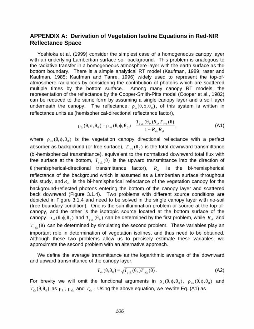
106

APPENDIX A: Derivation of Vegetation Isoline Equations in Red-NIRReflectance Space

Yoshioka et al. (1999) consider the simplest case of a homogeneous canopy layerwith an underlying Lambertian surface soil background. This problem is analogous tothe radiative transfer in a homogeneous atmosphere layer with the earth surface as thebottom boundary. There is a simple analytical RT model (Kaufman, 1989; raser andKaufman, 1985; Kaufman and Tanre, 1996) widely used to represent the top-of-atmosphere radiances by considering the contribution of photons which are scatteredmultiple times by the bottom surface. Among many canopy RT models, therepresentation of the reflectance by the Cooper-Smith-Pitts model (Cooper et al., 1982)can be reduced to the same form by assuming a single canopy layer and a soil layerunderneath the canopy. The reflectance, ),,( 0θϕθρλ , of this system is written inreflectance units as (hemispherical-directional reflectance factor),

λλ

λ↑λλ↓λλ −

θθ+θϕθρ=θϕθρ

sv

vsvv RR

TRT

1

)()(),,(),,( 0

00 , (A1)

where ),,( 0θϕθρ λv is the vegetation canopy directional reflectance with a perfect

absorber as background (or free surface), )( 0θλ↓vT is the total downward transmittance

(bi-hemispherical transmittance), equivalent to the normalized downward total flux withfree surface at the bottom, )(θλ↑v

T is the upward transmittance into the direction of

θ (hemispherical-directional transmittance factor), λsR is the bi-hemisphericalreflectance of the background which is assumed as a Lambertian surface throughoutthis study, and λvR is the bi-hemispherical reflectance of the vegetation canopy for thebackground-reflected photons entering the bottom of the canopy layer and scatteredback downward (Figure 3.1.4). Two problems with different source conditions aredepicted in Figure 3.1.4 and need to be solved in the single canopy layer with no-soil(free boundary condition). One is the sun illumination problem or source at the top-of-canopy, and the other is the isotropic source located at the bottom surface of thecanopy. ),,( 0θϕθρ λv and )( 0θλ↓v

T can be determined by the first problem, while λvR and

)(θλ↑vT can be determined by simulating the second problem. These variables play an

important role in determination of vegetation isolines, and thus need to be obtained.Although these two problems allow us to precisely estimate these variables, weapproximate the second problem with an alternative approach.

We define the average transmittance as the logarithmic average of the downwardand upward transmittance of the canopy layer,

)()(),( 00 θθ=θθ λ↑λ↓λ vvv TTT . (A2)

For brevity we will omit the functional arguments in ),,( 0θϕθρλ , ),,( 0θϕθρ λv and

),( 0θθλvT as λρ , λρv and λvT . Using the above equation, we rewrite Eq. (A1) as

107

λλ

λλλλ −

+ρ=ρsv

svv RR

RT

1

2

. (A3)

The first term of the right hand side (RHS) in Eq. (A3) is the reflectance contributionof only the vegetation canopy, i.e., the photons represented in this term never see thebackground. This value can be obtained by simply simulating the single-layer problemwith a free surface boundary condition (or black surface). The second RHS termrepresents the contribution of multiple scattering (interaction) between the soil surfaceand the canopy layer. The numerator represents first-order soil-vegetation interactionswhile the denominator is a result of higher order interaction terms. Our next step is toseparate the first order interaction term from the higher term by expansion of Eq.(A3)with a Taylor series,

22

222

1

λλλλ

λλ

λλλλλλλ

++ρ=

−++ρ=ρ

ORT

RR

RRTRT

svv

sv

vsvsvv

, (A4)

where

λλ

λλλλ

sv

svv

RR

RRTO

−=

1

222 . (A5)

In order to proceed, we rewrite Eq. (A4) for the red and NIR bands using the notation ofR and N instead of λ ,

22NsNvNvNN ORT ++ρ=ρ , and (A6)

22RsRvRvRR ORT ++ρ=ρ . (A7)

We can couple these equations with the soil line equation, which is the relationshipbetween the red and NIR reflectances for bare soil,

baRR sRsN += , (A8)

where a and b are the soil constants. We can eliminate the soil reflectances, sNR and

sRR , from Eqs. (A6)-(A8) to derive the vegetation isoline equation which is therelationship between the red and NIR reflectances. Using the following new definitions,the vegetation isoline equation becomes

2ODa RN ++γρ=ρ , (A9)

where the definitions of the variables used in the above are already introduced in 3.1.3.

We describe four steps to derive a vegetation isoline through use of a numericalradiative transfer model. We note that the numerical simulation model is only used todetermine the transmittance and reflectance properties of the canopy layer separatelyfrom the soil layer. The essence of this technique is to obtain the vegetation isolineparameters, λ and D , which are defined by Eqs. (4a) and (4b). To determine these

108

two parameters we need the following parameters, vRT , vNT , vNρ , vRρ . vRR , and vNR arealso needed to assess truncation of the higher order terms. We conduct twosimulations for each band per canopy LAI with two canopy background reflectances (asboundary conditions). The first simulation is with the free surface or perfect absorber(the black soil). For the second simulation, any background can be used. Although thechoice of the background for the second simulation is quite arbitrary, as we will see,darker backgrounds result in less error with the proposing technique. Since vRT , vNT ,

vNρ , vRρ , vRR , and vNR are purely functions of the canopy optical properties, we candetermine these values regardless of the actual soil optical properties. The schematicprocedure is summarized in Figure A1.

For this study we arbitrarily chose reflectances of 0.4 and 0.2 for red and NIR soilhemispherical reflectances. This pair which is on the line of sRsN RR 5.0= is very far fromthe soil lines used in this study, whose slope and intercept are chosen to 1.2 and 0.04respectively (Baret and Guyot, 1991). However, we chose these values to demonstratethat the vegetation isoline can be derived without knowledge of ‘actual’ soil reflectance.The details of four-step procedure for vegetation isoline derivation are summarizedbelow, and the flow chart of the procedure is shown in Figure A1.

Step 1 Parameter set up:

The first step is to choose a set of canopy parameters to run a numerical simulationcode. The parameters include LAI and any other optical properties of the canopy suchas leaf angle distribution (LAD) and leaf transmittance and reflectance. Also includedare sun and view angle conditions.

Step 2 Canopy RT simulation with the perfect absorber as the background:

The second step is the simulation of the canopy reflectance with the perfectabsorber as the boundary condition. This simulation corresponds to setting 0.0=λsR in

Eq. (A3) so that the result of this simulation is equal to λρv .

Step 3 Canopy RT simulation with an arbitrary background:

The third step is the canopy simulation with an arbitrary background. Although thechoice of the soil reflectance values is arbitrary, the values must be small enough tomake the following approximation of average transmittance valid. Eq. (A3) is solvedabout 2

λvT as,

λλλλλλ −ρ−ρ= ssvvv RRRT /)1)((2 , (A10)

where λρ is the result of the simulation executed in this step and λρv is the canopyreflectance obtained by the previous black soil step. We still do not know the canopybi-hemispherical reflectance at the bottom surface of the canopy (for the photonsentering the canopy layer from the bottom surface and reflected toward the soil), but wecan approximate this value by λρv . This approximation may be drastic, however, it

109

becomes insignificant if we choose a small value for λsR . Before we show this, werewrite the above equation with the approximation:

λλλλλλ ρ−ρ−ρ≈ ssvvv RRT /)1)((2 . (A11)

The only difference of the above two equations is that the factor of )1( λλ− sv RR is

approximated by )1( λλρ− sv R . This approximation would be insignificant regardless of

the approximation of λvR by λρv if both λλ sv RR and λλρ− sv R1 are smaller than 0.1(comparing to 1.0). In order to keep these values smaller than 0.1, we must choose asmall value for λsR which is the input of the simulation done in this step. By choosing

0.4 for the red band, the value of λλ sv RR for this band will be smaller than 0.04 since

both λvR and λρv of red band are normally lower than 0.1. On the other hand, for the

NIR band both λvR and λρv are expected to be as high as 0.5. By choosing 0.2 for λsR

we can keep the value of λλ sv RR to be smaller than 0.1. Thus the error in the estimation

of 2λvT associated with the approximation of λvR by λρv is approximately one order

smaller than the original error. For example, if we assume that λρv of 0.5 is used for

λvR whose true value is 0.3, then the approximation is affected by 0.04, which is much

smaller than (1.0-0.3×0.2)=0.94 on the estimation of 2λvT .

Although it is better to choose smaller values of λsR for each band in this simulationto make the above approximation relatively insignificant, the choice of too small a valuealso causes error on the 2

λvT estimation. The reason is that the numerical canopymodel used for this step (and the previous step) has its own accuracy limitations. Sincewe have a subtraction term, )( λλ ρ−ρ v , the numerical error of the model in these two

values may be enhanced if we choose a very small value for λsR . The difference of λρand λρv will be negligible if we chose too small a value of λsR .

Step 4 Determination of the vegetation isoline parameters:

We finally determine the vegetation isoline parameters, γ and D , by using vNρ , vRρ ,

vNT and vRT obtained from steps 2 and 3. γ is computed by using Eq. (4a) which is

totally independent of the soil line parameters. D , ND and RD are then computed from

Eqs. (4b), (4c) and (4d). Although D and ND are functions of the soil line parameters,

other terms and factors ( vNρ , vRρ , vNT , and γ ) are completely independent of the soilparameters a and b. Therefore, we can execute the previous three steps withoutknowledge of actual soil properties. Thus, we do not need to repeat steps 1-3 for thedifferent soil parameters if the canopy and LAI are the same. We just need to repeatstep 4 to compute the vegetation isoline for a different set of soil line parameters.

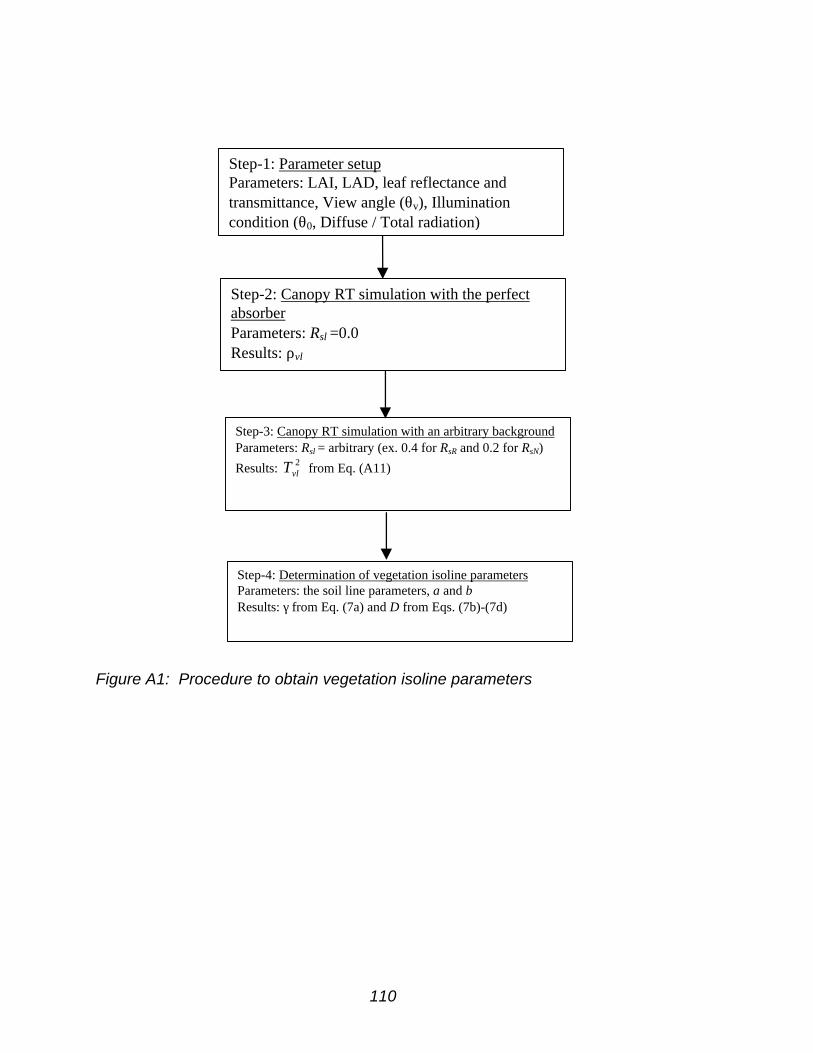
110

Figure A1: Procedure to obtain vegetation isoline parameters

Step-1: Parameter setupParameters: LAI, LAD, leaf reflectance andtransmittance, View angle (θv), Illuminationcondition (θ0, Diffuse / Total radiation)

Step-2: Canopy RT simulation with the perfectabsorberParameters: Rsλ=0.0Results: ρvλ

Step-3: Canopy RT simulation with an arbitrary backgroundParameters: Rsλ= arbitrary (ex. 0.4 for RsR and 0.2 for RsN)

Results: 2λvT from Eq. (A11)

Step-4: Determination of vegetation isoline parametersParameters: the soil line parameters, a and bResults: γ from Eq. (7a) and D from Eqs. (7b)-(7d)

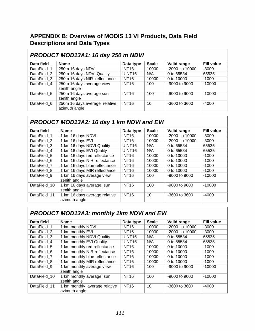
111

APPENDIX B: Overview of MODIS 13 VI Products, Data FieldDescriptions and Data Types

PRODUCT MOD13A1: 16 day 250 m NDVIData field Name Data type Scale Valid range Fill valueDataField_1 250m 16 days NDVI INT16 10000 -2000 to 10000 -3000DataField_2 250m 16 days NDVI Quality UINT16 N/A 0 to 65534 65535DataField_3 250m 16 days NIR reflectance INT16 10000 0 to 10000 -1000DataField_4 250m 16 days average view

zenith angleINT16 100 -9000 to 9000 -10000

DataField_5 250m 16 days average sunzenith angle

INT16 100 -9000 to 9000 -10000

DataField_6 250m 16 days average relativeazimuth angle

INT16 10 -3600 to 3600 -4000

PRODUCT MOD13A2: 16 day 1 km NDVI and EVIData field Name Data type Scale Valid range Fill valueDataField_1 1 km 16 days NDVI INT16 10000 -2000 to 10000 -3000DataField_2 1 km 16 days EVI INT16 10000 -2000 to 10000 -3000DataField_3 1 km 16 days NDVI Quality UINT16 N/A 0 to 65534 65535DataField_4 1 km 16 days EVI Quality UINT16 N/A 0 to 65534 65535DataField_5 1 km 16 days red reflectance INT16 10000 0 to 10000 -1000DataField_6 1 km 16 days NIR reflectance INT16 10000 0 to 10000 -1000DataField_7 1 km 16 days blue reflectance INT16 10000 0 to 10000 -1000DataField_8 1 km 16 days MIR reflectance INT16 10000 0 to 10000 -1000DataField_9 1 km 16 days average view

zenith angleINT16 100 -9000 to 9000 -10000

DataField_10 1 km 16 days average sunzenith angle

INT16 100 -9000 to 9000 -10000

DataField_11 1 km 16 days average relativeazimuth angle

INT16 10 -3600 to 3600 -4000

PRODUCT MOD13A3: monthly 1km NDVI and EVIData field Name Data type Scale Valid range Fill valueDataField_1 1 km monthly NDVI INT16 10000 -2000 to 10000 -3000DataField_2 1 km monthly EVI INT16 10000 -2000 to 10000 -3000DataField_3 1 km monthly NDVI Quality UINT16 N/A 0 to 65534 65535DataField_4 1 km monthly EVI Quality UINT16 N/A 0 to 65534 65535DataField_5 1 km monthly red reflectance INT16 10000 0 to 10000 -1000DataField_6 1 km monthly NIR reflectance INT16 10000 0 to 10000 -1000DataField_7 1 km monthly blue reflectance INT16 10000 0 to 10000 -1000DataField_8 1 km monthly MIR reflectance INT16 10000 0 to 10000 -1000DataField_9 1 km monthly average view

zenith angleINT16 100 -9000 to 9000 -10000

DataField_10 1 km monthly average sunzenith angle

INT16 100 -9000 to 9000 -10000

DataField_11 1 km monthly average relativeazimuth angle

INT16 10 -3600 to 3600 -4000

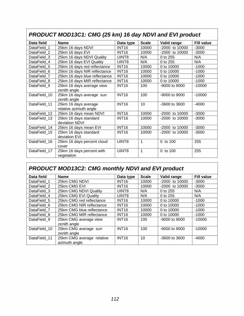
112

PRODUCT MOD13C1: CMG (25 km) 16 day NDVI and EVI productData field Name Data type Scale Valid range Fill valueDataField_1 25km 16 days NDVI INT16 10000 -2000 to 10000 -3000DataField_2 25km 16 days EVI INT16 10000 -2000 to 10000 -3000DataField_3 25km 16 days NDVI Quality UINT8 N/A 0 to 255 N/ADataField_4 25km 16 days EVI Quality UINT8 N/A 0 to 255 N/ADataField_5 25km 16 days red reflectance INT16 10000 0 to 10000 -1000DataField_6 25km 16 days NIR reflectance INT16 10000 0 to 10000 -1000DataField_7 25km 16 days blue reflectance INT16 10000 0 to 10000 -1000DataField_8 25km 16 days MIR reflectance INT16 10000 0 to 10000 -1000DataField_9 25km 16 days average view

zenith angleINT16 100 -9000 to 9000 -10000

DataField_10 25km 16 days average sunzenith angle

INT16 100 -9000 to 9000 -10000

DataField_11 25km 16 days averagerelative azimuth angle

INT16 10 -3600 to 3600 -4000

DataField_12 25km 16 days mean NDVI INT16 10000 -2000 to 10000 -3000DataField_13 25km 16 days standard

deviation NDVIINT16 10000 -2000 to 10000 -3000

DataField_14 25km 16 days mean EVI INT16 10000 -2000 to 10000 -3000DataField_15 25km 16 days standard

deviation EVIINT16 10000 -2000 to 10000 -3000

DataField_16 25km 16 days percent cloudcover

UINT8 1 0 to 100 255

DataField_17 25km 16 days percent withvegetation

UINT8 1 0 to 100 255

PRODUCT MOD13C2: CMG monthly NDVI and EVI productData field Name Data type Scale Valid range Fill valueDataField_1 25km CMG NDVI INT16 10000 -2000 to 10000 -3000DataField_2 25km CMG EVI INT16 10000 -2000 to 10000 -3000DataField_3 25km CMG NDVI Quality UINT8 N/A 0 to 255 N/ADataField_4 25km CMG EVI Quality UINT8 N/A 0 to 255 N/ADataField_5 25km CMG red reflectance INT16 10000 0 to 10000 -1000DataField_6 25km CMG NIR reflectance INT16 10000 0 to 10000 -1000DataField_7 25km CMG blue reflectance INT16 10000 0 to 10000 -1000DataField_8 25km CMG MIR reflectance INT16 10000 0 to 10000 -1000DataField_9 25km CMG average view

zenith angleINT16 100 -9000 to 9000 -10000

DataField_10 25km CMG average sunzenith angle

INT16 100 -9000 to 9000 -10000

DataField_11 25km CMG average relativeazimuth angle

INT16 10 -3600 to 3600 -4000

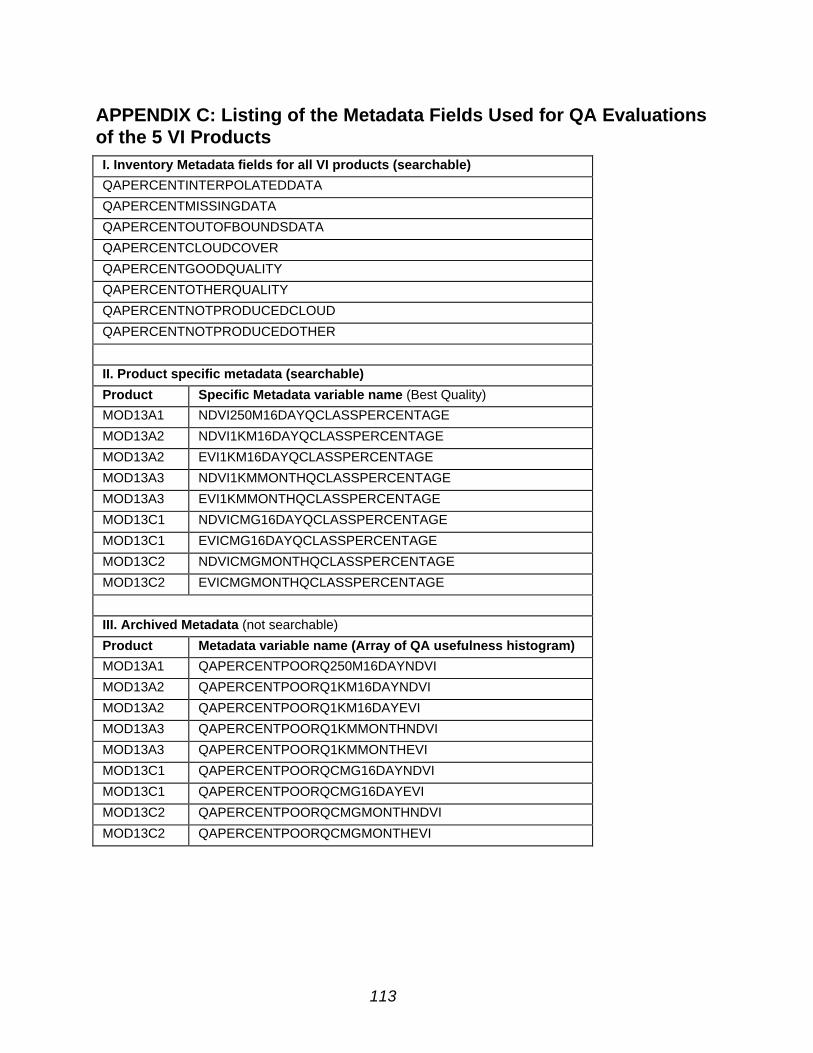
113

APPENDIX C: Listing of the Metadata Fields Used for QA Evaluationsof the 5 VI ProductsI. Inventory Metadata fields for all VI products (searchable)

QAPERCENTINTERPOLATEDDATA

QAPERCENTMISSINGDATA

QAPERCENTOUTOFBOUNDSDATA

QAPERCENTCLOUDCOVER

QAPERCENTGOODQUALITY

QAPERCENTOTHERQUALITY

QAPERCENTNOTPRODUCEDCLOUD

QAPERCENTNOTPRODUCEDOTHER

II. Product specific metadata (searchable)

Product Specific Metadata variable name (Best Quality)

MOD13A1 NDVI250M16DAYQCLASSPERCENTAGE

MOD13A2 NDVI1KM16DAYQCLASSPERCENTAGE

MOD13A2 EVI1KM16DAYQCLASSPERCENTAGE

MOD13A3 NDVI1KMMONTHQCLASSPERCENTAGE

MOD13A3 EVI1KMMONTHQCLASSPERCENTAGE

MOD13C1 NDVICMG16DAYQCLASSPERCENTAGE

MOD13C1 EVICMG16DAYQCLASSPERCENTAGE

MOD13C2 NDVICMGMONTHQCLASSPERCENTAGE

MOD13C2 EVICMGMONTHQCLASSPERCENTAGE

III. Archived Metadata (not searchable)

Product Metadata variable name (Array of QA usefulness histogram)

MOD13A1 QAPERCENTPOORQ250M16DAYNDVI

MOD13A2 QAPERCENTPOORQ1KM16DAYNDVI

MOD13A2 QAPERCENTPOORQ1KM16DAYEVI

MOD13A3 QAPERCENTPOORQ1KMMONTHNDVI

MOD13A3 QAPERCENTPOORQ1KMMONTHEVI

MOD13C1 QAPERCENTPOORQCMG16DAYNDVI

MOD13C1 QAPERCENTPOORQCMG16DAYEVI

MOD13C2 QAPERCENTPOORQCMGMONTHNDVI

MOD13C2 QAPERCENTPOORQCMGMONTHEVI

114

APPENDIX D: QA Flag Key and DescriptionSpatial and temporalresolution

250m16 days

1km/16days 1km/monthly. CMG/16days CMG/monthly.

Parameter # bits NDVI NDVI EVI NDVI EVI NDVI EVI NDVI EVI Quality 2 0-1 0-1 0-1 0-1 0-1 0-1 0-1 0-1 0-1 Usefulness 4 2-5 2-5 2-5 2-5 2-5 2-5 2-5 2-5 2-5 Aerosol 2 6-7 6-7 6-7 6-7 6-7 6-7 6-7 6-7 6-7 Adj. corr. 1 8 8 8 8 8 Atm. corr. 1 9 9 9 9 9 Mixed Clouds 1 10 10 10 10 10 Land/Water 2 11-12 11-12 11-12 11-12 11-12 Snow/Ice 1 13 13 13 13 13 Shadow 1 14 14 14 -- -- Mixed Comp. 1 -- -- -- 14 14 Comp.Method

1 15 15 15 15 15

Key to bit positions:Bit Parameter Description0-1 VI quality

(MODLAND)01 VI produced, but check QA00 VI produced, good quality;10 pixel not produced due to cloud effects11 pixel not produced due to other reasons than clouds

2-5 VI usefulness 0= highest quality,…., 7=intermediate quality, …,13=lowest quality,14= quality too low to be useful, 15= not useful for any other reason(clouds)

6-7 Aerosol quantity :00 climatology, 01 low, 10 average , 11 high8 Atmosphere Adjacency

correction:0 no adjacency correction; 1 adjacency effect corrected

9 Atm. corr. 0 (no) 1 (yes) atmosphere BRDF correction performed10 Mixed Clouds 0 no; 1 yes mixed clouds11-12 Land/Water 00 Ocean/water; 01 Coast; 10 Wetland; 11 Land

Where these four land /water categories were assigned one or more of the following descriptions:Ocean/water: 0. Shallow Ocean (Ocean <5k from coast OR <50m deep; i.e., a buffer zone

around all coastal areas and islands, plus shallow areas up to 50m deep that arefurther than 5 km from the land). Includes the appropriate parts of the Black Sea,Red Sea, Mediterranean Sea, Hudson Bay, and other ocean-connected seas.

Land 1. Land (not anything else).Coast: 2. Ocean Coastlines and Lake Shorelines (an actual boundary line).

Coast: 3. Shallow Inland Water (Inland water<5km from shoreline or <50 m deep;i.e..a buffer zone around all lake shores and inland islands, plus shallow areas up to50m deep that are further than 5km from the land). Includes the appropriateparts of the Caspian Sea, Aral Sea, Great Lakes, 2-line rivers, etc.

Wetland: 4. Ephemeral (intermittent) Water (from Digital Chart of the World).Ocean/Water: 5. Deep Inland Water (Inland water >5 km from shoreline AND >50m deep;

i.e., Lake waters beyond 5 km from their shore or islands, and greater than 50mdeep). Includes the appropriate parts of the Caspian Sea, Aral Sea, GreatLakes, etc.

Ocean/Water: 6. Moderate and continental ocean

115

Ocean/Water: 7. Deep Ocean (Ocean >5km from coast AND >50m deep); i.e., Oceansbeyond 5km from coastal areas and islands, and greater than 50m deep).Includes the appropriate parts of the Black Sea, Red Sea, Mediterranean Sea,Hudson Bay, and other ocean-connected seas.

13 Snow/Ice 0 no; 1 yes possible snow/ice14 Shadow 0 no; 1 yes possible shadow14 Mixed

Composite(1km monthlyonly):

0 no; 1 yes mixed composite methods used in monthly composite

15 Comp. Method 0 BRDF model based nadir equivalent VI1 CVMVC (constraint view angle maximum value VI)

116

APPENDIX E: Usefulness Scale Interpretation Key for MODIS 13ProductsMarks (rating scheme) to be summed for each 250 m and 1 km pixel:(Take the worst case scenario from day to day; Post launch revisions are expected)

Parameter Rating (mark)Aerosol quantity based on 1 km data:climatology Mark 2low mark 0average mark 0high mark 3

no adjacency correction. mark 1 (Not applicable for 1km product)no atm. BRDF correction. mark 2

Mixed clouds mark 3Possible shadow mark 2

VIEW angle >40° mark 1SUNANGLE >60° mark 1

VI usefulness scale for CMG 16 day composite:Usefulness Description0 highest quality12-6 undefined7 intermediate quality8910 low quality (76-99% clouds and high aerosols)1112 lowest quality (76-99% clouds and high aerosols, view and sun angle)13 uncertain about quality (if not determined; default)14 quality too low to be useful15 not useful for any other reason (clouds etc)

Marks (rating) to be summed for each CMG pixel to compute the usefulness index:Parameter: Rating (marks)Aerosol quantity based on 1 km data (take worst case scenario):climatology mark 1low mark 0average mark 0high mark 6

percentage clouds inside CMG pixel1-25 mark 126-50 mark 151-75 mark 276-99 mark 4

VIEW angle >40° mark 1SUNANGLE >60° mark 1

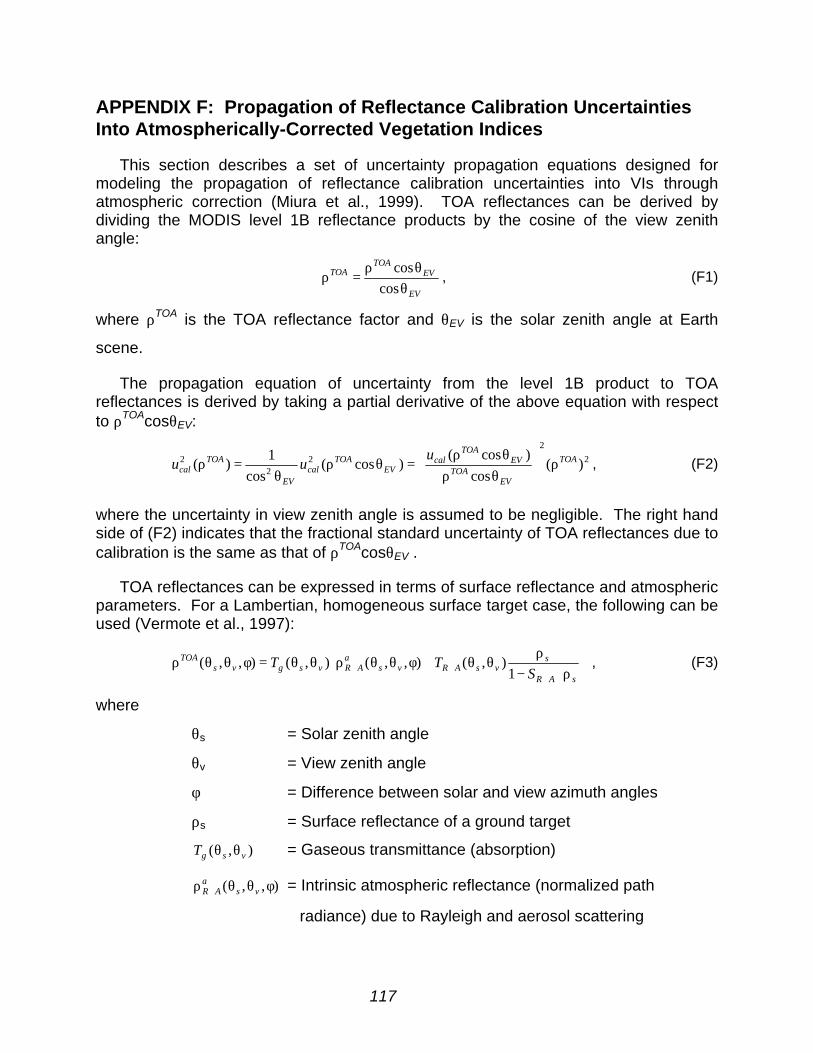
117

APPENDIX F: Propagation of Reflectance Calibration UncertaintiesInto Atmospherically-Corrected Vegetation Indices

This section describes a set of uncertainty propagation equations designed formodeling the propagation of reflectance calibration uncertainties into VIs throughatmospheric correction (Miura et al., 1999). TOA reflectances can be derived bydividing the MODIS level 1B reflectance products by the cosine of the view zenithangle:

EV

EVTOA

TOA

θθρ

=ρcos

cos, (F1)

where ρTOA is the TOA reflectance factor and θEV is the solar zenith angle at Earth

scene.

The propagation equation of uncertainty from the level 1B product to TOAreflectances is derived by taking a partial derivative of the above equation with respectto ρTOAcosθEV:

2

2

22

2 )(cos

)cos()cos(

cos

1)( TOA

EVTOA

EVTOA

calEV

TOAcal

EV

TOAcal

uuu ρ

θρθρ

=θρθ

=ρ , (F2)

where the uncertainty in view zenith angle is assumed to be negligible. The right handside of (F2) indicates that the fractional standard uncertainty of TOA reflectances due tocalibration is the same as that of ρTOAcosθEV .

TOA reflectances can be expressed in terms of surface reflectance and atmosphericparameters. For a Lambertian, homogeneous surface target case, the following can beused (Vermote et al., 1997):

ρ⋅−

ρθθ+φθθρθθ=φθθρ

+++

sAR

svsARvs

aARvsgvs

TOA

STT

1),(),,(),(),,( , (F3)

where

θs = Solar zenith angle

θv = View zenith angle

φ = Difference between solar and view azimuth angles

ρs = Surface reflectance of a ground target

),( vsgT θθ = Gaseous transmittance (absorption)

),,( φθθρ + vsa

AR = Intrinsic atmospheric reflectance (normalized path

radiance) due to Rayleigh and aerosol scattering

118

),( vsART θθ+ = Two-way atmospheric transmittance due to Rayleigh and

aerosol scattering

ARS + = Spherical albedo due to Rayleigh and aerosol scattering.

Thus, atmospherically-corrected surface reflectance ρac is derived by solving (F3) for ρs:

ARac

acac

S +ρ+ρ

=ρ*

*

1, (F4)

where

AR

aARTac

Tg

TOA

+

+ρ ρ−

=ρ * . (F4a)

The standard uncertainty in ρTOA will propagate to ρac and the uncertaintypropagation equation is derived by taking a partial derivative of (F4) with respect toρTOA:

)()( 2

2

2 TOAcalTOA

acac

cal uu ρ

ρ∂ρ∂

=ρ , (F5)

where

ρ−+=

ρ∂ρ∂

+++

+ρ

ARgARAR

aART

TOA

ac

TTST

g

TOA

11 . (F5a)

The partial derivative or sensitivity coefficient (F5a) includes both ρTOA and atmosphericparameters used for atmospheric correction, indicating that the standard uncertainty inρac changes with both atmospheric conditions and surface reflectances. It should benoted that the uncertainty propagation equation here (F5) propagates reflectancecalibration uncertainty and assumes the uncertainty in atmospheric corrections to benegligible.

VIs can then be calculated from the surface reflectances. For the NDVI:

redNIR

redNIRNDVIρ+ρρ−ρ

= , (F6)

the uncertainty propagation equation is derived by taking partial derivatives of (F6) with

respect to the red and NIR reflectances:

),(2)()()( 2

2

2

2

2redNIRcal

redNIRredcal

redNIRcal

NIRcal u

NDVINDVIu

NDVIu

NDVINDVIu ρρ

∂ρ∂

∂ρ∂

+ρ

∂ρ

∂+ρ

∂ρ

∂= , (F7)

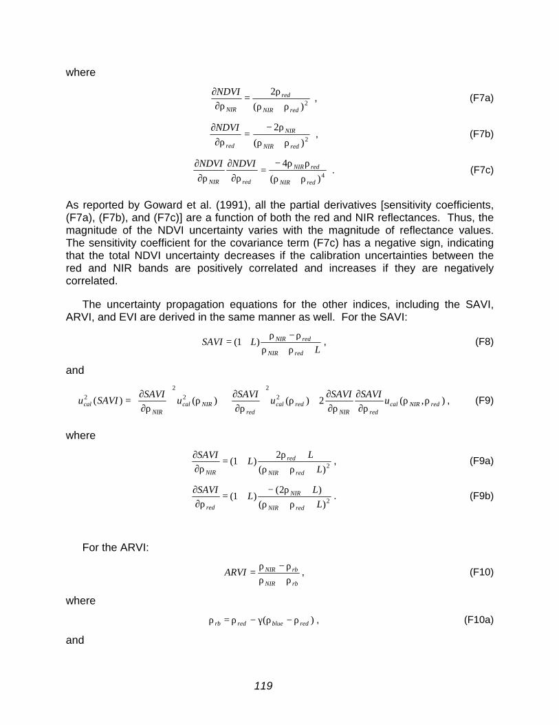
119

where

2)(

2

redNIR

red

NIR

NDVI

ρ+ρρ

=∂ρ

∂ , (F7a)

2)(

2

redNIR

NIR

red

NDVI

ρ+ρ

ρ−=

∂ρ∂

, (F7b)

4)(

4

redNIR

redNIR

redNIR

NDVINDVI

ρ+ρ

ρρ−=

∂ρ∂

∂ρ∂

. (F7c)

As reported by Goward et al. (1991), all the partial derivatives [sensitivity coefficients,(F7a), (F7b), and (F7c)] are a function of both the red and NIR reflectances. Thus, themagnitude of the NDVI uncertainty varies with the magnitude of reflectance values.The sensitivity coefficient for the covariance term (F7c) has a negative sign, indicatingthat the total NDVI uncertainty decreases if the calibration uncertainties between thered and NIR bands are positively correlated and increases if they are negativelycorrelated.

The uncertainty propagation equations for the other indices, including the SAVI,ARVI, and EVI are derived in the same manner as well. For the SAVI:

LLSAVI

redNIR

redNIR

+ρ+ρρ−ρ

+= )1( , (F8)

and

),(2)()()( 2

2

2

2

2redNIRcal

redNIRredcal

redNIRcal

NIRcal u

SAVISAVIu

SAVIu

SAVISAVIu ρρ

∂ρ∂

∂ρ∂

+ρ

∂ρ∂

+ρ

∂ρ∂

= , (F9)

where

2)(

2)1(

L

LL

SAVI

redNIR

red

NIR +ρ+ρ+ρ

+=∂ρ∂

, (F9a)

2)(

)2()1(

L

LL

SAVI

redNIR

NIR

red +ρ+ρ+ρ−

+=∂ρ

∂. (F9b)

For the ARVI:

rbNIR

rbNIRARVIρ+ρρ−ρ

= , (F10)

where

)( redblueredrb ρ−ργ−ρ=ρ , (F10a)

and

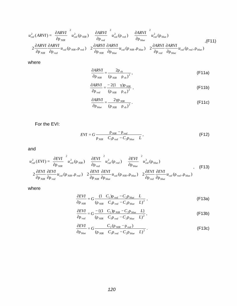
120

),(2),(2),(2

)()()()( 2

2

2

2

2

2

2

blueredcalbluered

blueNIRcalblueNIR

redNIRcalredNIR

bluecalblue

redcalred

NIRcalNIR

cal

uARVIARVI

uARVIARVI

uARVIARVI

uARVI

uARVI

uARVI

ARVIu

ρρ∂ρ∂

∂ρ∂

+ρρ∂ρ∂

∂ρ∂

+ρρ∂ρ

∂∂ρ∂

+

ρ

∂ρ∂

+ρ

∂ρ

∂+ρ

∂ρ∂

=,(F11)

where

2)(

2

rbNIR

rb

NIR

ARVI

ρ+ρρ

=∂ρ∂

, (F11a)

2)(

)1(2

rbNIR

NIR

red

ARVI

ρ+ρργ+−

=∂ρ

∂, (F11b)

2)(

2

rbNIR

NIR

blue

ARVI

ρ+ργρ

=∂ρ∂

. (F11c)

For the EVI:

LCCGEVI

blueredNIR

redNIR

+ρ−ρ+ρρ−ρ

=21

, (F12)

and

),(2),(2),(2

)()()()( 2

2

2

2

2

2

2

blueredcalbluered

blueNIRcalblueNIR

redNIRcalredNIR

bluecalblue

redcalred

NIRcalNIR

cal

uEVIEVI

uEVIEVI

uEVIEVI

uEVI

uEVI

uEVI

EVIu

ρρ∂ρ∂

∂ρ∂

+ρρ∂ρ∂

∂ρ∂

+ρρ∂ρ∂

∂ρ∂

+

ρ

∂ρ∂

+ρ

∂ρ∂

+ρ

∂ρ∂

=, (F13)

where

221

21

)(

)1(

LCC

LCCG

EVI

blueredNIR

bluered

NIR +ρ−ρ+ρ+ρ−ρ+

=∂ρ∂

, (F13a)

221

21

)(

})1{(

LCC

LCCG

EVI

blueredNIR

blueNIR

red +ρ−ρ+ρ+ρ−ρ+−

=∂ρ∂

, (F13b)

221

2

)(

)(

LCC

CG

EVI

blueredNIR

redNIR

blue +ρ−ρ+ρρ−ρ

=∂ρ∂

. (F13c)