NCDC Technical Report

NCDC No. GHCNM-12-02

Modifications to Pairwise

Homogeneity Adjustment

software to address coding

errors and improve run-time

efficiency

Claude Williams

Matt Menne

Jay Lawrimore

NOAA’s National Climatic Data Center

Asheville, NC

August 1, 2012

This report, GHCNM-12-02, provides descriptions of software modifications made

and implemented in GHCN-Monthly version 3.2.0.

U.S. DEPARTMENT OF COMMERCE

National Oceanic and Atmospheric Administration

National Climatic Data Center

Asheville, NC 28801-5001

Table of Contents

List of Acronyms………………………………………………………………….i

Abstract…...………………………………………………………………………1

1. Introduction ........................................................................................................... 2

2. Software Modifications .......................................................................................... 5

a. Modify debugging options and initialization counters

b. Change in scripts due to asynchronous execution problems

c. Standard Normal Homogeniety test: number of observations

d. Kendall-Thiel Paired-slope function: looping index

e. Kendall-Thiel Paired-slope function: x-axis median

f. Kendall-Thiel Paired-slope function: number of observations

g. BIC Sloped vs. TPR0 test: number of observations

h. Semi-hierarchical Segmentation function “corner case”

3. Changes to global anomalies and trends ................................................................ 9

4. Conclusions………………………………………………………………………12

5. References……………………………………………………………………......13

Tables:

Table 1: Number of Positive/Negative/Total Changepoints………………………..14

Figures:

• Figure 1: Histogram of magnitude of bias correction…………………………….15

• Figure 2: Percent of stations for which bias corrections were applied……………18

• Figure 3: Global mean temperatures before and after software changes………….19

• Figure 4: Global annual average land surface temperature anomalies…………….23

• Figure 5: Maps of 5X5 grid box annual temperature trends (1901-2011)…………24

• Figure 6: Maps of 5X5 grid box annual temperature trends (1951-2011)..………..25

• Figure 7: Individual station series with large changes in trend……………………26

List of Acronyms

BIC: Bayesian Information Criteria

GHCN-M: Global Historical Climatology Network-Monthly

NCDC: National Climatic Data Center

NOAA: National Oceanic and Atmospheric Administration

PHA: Pairwise Homogeneity Adjustment

USHCN: U.S. Historical Climatology Network

1

Abstract

The software used to perform operational updates and reprocessing of GHCN-M version 3 was

modified to correct software coding errors and to improve its run-time efficiency. In particular,

errors in the Pairwise Homogenization Algorithm (PHA) were identified during the course of a

project led by Mr. Daniel Rothenberg in July 2011 that was undertaken as part of Google’s

“Summer of Code” and supervised by the Climate Code Foundation (with collaboration by

NOAA/NCDC). The errors and steps taken to correct each error are described in this technical

report. In addition, changes were made to improve debugging and data processing efficiency. A

comparison of U.S. and global analyses performed using the PHA software before and after the

corrections and modifications are included. With the software corrections the sensitivity of the

PHA improved, resulting in an approximate two-fold increase in the frequency of bias

adjustments applied globally. The impact on annual means resulted in a change in century-scale

global land surface air temperature trends of approximately 0.01°C/decade. The software

modifications are incorporated into a new release of GHCN-M, version 3.2.0.

2

1. Introduction

The Global Historical Climatology Network-Monthly (GHCN-M) version 3.0.0 dataset was

released to the public in May 2011. Subsequent modifications were implemented to improve

processing speed through improvements to processing data within sparse matrices. This change

was implemented as version 3.1.0 in November 2011 (NOAA Tech Report GHCNM-12-01R).

Changes described in this report primarily involve changes to the Pairwise Homogenization

Algorithm (PHA; Menne and Williams 2009) software that correct coding errors that reduced the

algorithm’s efficiency in identifying inhomogeneities in the GHCN monthly temperature series.

The nature of the homogeneity adjustments made to remove non-climatic influences that can bias

the GHCN-M temperature record are described in Lawrimore et al. 2011 for version 3.0.0. In

brief, adjustments are necessary because surface weather stations are frequently subject to minor

relocations throughout their history of operation and may also undergo changes in

instrumentation as measurement technology evolves. Furthermore, observing practices may vary

through time, and the land use/land cover in the vicinity of an observing site can be altered by

either natural or man-made causes. Any such modifications to the circumstances behind

temperature measurements have the potential to alter a thermometer’s microclimate exposure

characteristics or otherwise change the bias of measurements relative to those taken under

previous circumstances. The manifestation of such changes is often an abrupt shift in the mean

level of temperature readings that is unrelated to true climate variations and trends. Ultimately,

these artifacts (also known as inhomogeneities) confound attempts to quantify climate variability

3

and change because the magnitude of the artifact can be as large as or larger than the true

background climate signal. The process of removing the impact of non-climatic changes in

climate series is called homogenization.

In version 3 of the GHCN-M temperature data, the apparent impacts of documented and

undocumented inhomogeneities are detected and corrected through automated pairwise

comparisons of mean monthly temperature series as detailed in Menne and Williams [2009]. This

method improved upon earlier methods in part because it did not rely on the creation of a

homogenous composite reference series from neighboring stations [Menne and Williams, 2005].

In implementing this method, minor software coding errors were made. These errors were

identified during the course of a collaborative project led by Mr. Daniel Rothenberg in July 2011.

Mr. Rothenberg was funded by the Google Summer of Code project to convert the PHA software

code from FORTRAN77 to Python. This was part of a larger effort of the Climate Code

Foundation to improve accessibility to climate related software. The errors and steps taken to

correct each error, referred to as “Roth bug fixes”, are described in this document. A comparison

of U.S. and global analyses performed using the software before and after the corrections is

included. The comparisons were first performed on an incremental basis to understand one by

one the impact of changes and corrections from those that were expected to have little impact on

global averages to those expected to have the greatest impact. The combined impact of all

changes and corrections compared against the previous version (3.1.0) was then assessed. These

4

changes, which are discussed in the following sections, are incorporated into a new release of

GHCN-M, version 3.2.0.

5

2. Software Modifications

Two very minor changes were made to improve debugging and processing efficiency.

a) Base 2: Changes to debugging options and initialization counters.

b) Base 2c: Change in scripts due to asynchronous execution problems associated with

processing monthly mean maximum temperature followed by monthly mean minimum

temperature. Also added was the ability to add new stations automatically when their

period of record increased enough to perform bias corrections and improved testing when

there are an insufficient number of neighbors to calculate adjustments.

The following modifications were made to the Pairwise Homogeneity Algorithm (Menne and

Williams, 2009). The reader is encouraged to review Menne and Williams (2009) or Williams et

al (2012) to better understand the following descriptions.

a) Roth bug fix 1: Kendall-Thiel Paired-slope function x-axis median

In comparisons with benchmarks (Williams et al, 2011), it was found that median

estimates provided by the non-parametric Kendall-Thiel function improved

approximations used to identify the magnitude of the offsets between segments. For the

TPR1 data model (constant slope with offset; Menne and Williams, 2009, Table 1), the Y-

median was correctly provided for the entire span of both segments, however the X-

6

median was only provided for the 2nd

segment. This coding change had no impact on

global averages and trends, because it was used only in the debugging log.

b) Roth bug fix 2: Semi-hierarchical Segmentation function “corner case”

The Bayesian Information Criteria (BIC) model selection was handled incorrectly in a

small number of cases (114 times out of 183,167 chances) where three or more breaks

were identified by the Standard Normal Homogeneity Test (SNHT) within 18

months. The BIC data model and residual error statistic are determined as if each

changepoint is the only one in the interval and the break whose model has the overall

minimum BIC (i.e. with the lowest residual error statistic) is chosen as the model fit for

the entire interval. The error was that if the model selected for the earliest break did not

include a step change (i.e., as a flat or sloped line), then this model was always used and

no break was retained.

c) Roth bug fix 3: Kendall-Thiel Paired-slope function looping index.

The Kendall-Thiel Paired-slope function is used to compare the slope of two segments of

temperature observations, one on each side of a potential discontinuity. It involves the use

of a symmetrical 2-dimensional array which is traversed to collect all of the paired

observations between the two segments. For one type of discontinuity (the “constant

slope with offset” (TPR1) data model), the looping index for the 1st segment correctly

scans just the upper triangle of the matrix. The looping index for the 2nd segment should

also have only scanned the upper triangle of the matrix, but it incorrectly scanned the

7

entire matrix. This had the impact of doubling the weight of the 2nd segment statistics in

later calculations, which biased this data model toward the attributes of the 2nd segment.

d) Roth bug fix 4: Kendall-Thiel Paired-slope function incorrectly assumed no missing data

in array.

The array index of the last observation passed from the routine to the Bayesian

Information Criteria function assumed the array to be serially complete, when it still had

embedded missing data. [The BIC is used to determine which of five models (Menne and

Williams, 2009; Table 1) provides the best representation for each changepoint. The

model that minimizes the BIC is selected as the best representation for each changepoint.]

The array index of the last observation in one of the five models (TPR1), assumed the

array to be serially complete when the missing data are still embedded in the array.

Again, not all of the available data were used. The impact was to degrade the TPR1 data

model statistics in the Bayesian model comparison by not using all of the available

observations.

e) Roth bug fix 5: Standard Normal Homogeneity Test (SNHT): array index of the last

observation.

As part of the SNHT, the index of the last observation for an array containing monthly

mean temperature is passed into a subroutine. This number limits the array elements

examined in the array and was incorrectly truncated. Not all available valid observations

were used in the test because of the truncated array. The impact of this coding error was a

8

reduction in the sensitivity of the breakpoint test because the number of observations in

the sample was undercounted (and thus the test-statistic value used to determine

statistical significance was too high). Because of this sample size error, some pairwise

breakpoints were not detected when they should have been.

f) Roth bug fix 6: Bayesian Information Criteria assessment of sloped line (SLR1) model

vs. shift in mean (TPR0) model: index for last observation.

To determine whether a break identified by the SNHT is better represented as a trend, the

BIC is used to determine whether a model representing two segments separated by a shift

might be more appropriately represented by a single sloped line. If the BIC suggests that

the better fit is a single sloped line, the changepoint dividing the two segments is

removed from consideration. The function call for the sloped data model was incorrect (it

assumed no missing data when there were missing data). The impact was to artificially

increase the likelihood of choosing the sloped line data model, thus reducing the ability to

find step-wise (TPR0) changepoints (Menne and Williams, 2009, Table 1).

9

3. Changes to global anomalies and trends

The improved sensitivity of the v3.2.0 algorithms led to changes in the adjusted station

series and the global average temperature. These changes resulted from identifying and adjusting

changepoints that had been unidentified in v3.1.0. Figure 1a, 1b and 1c show the frequency and

magnitude of bias corrections for both versions with respect to the GHCN Tavg, USHCN Tmin

and USHCN Tmax. Note that maximum and minimum temperature are corrected separately for

USHCN stations and mean temperature data are corrected for non-USHCN stations.

Table 1 further tabulates a comparison of v3.2.0 versus v3.1.0 corrections by data subset and

sign of correction. The greater sensitivity of v3.2.0 resulted in the detection of approximately

two times as many change points compared to v3.1.0. The average adjustment for the positive

and negative v3.2.0 changepoints are on average smaller than v3.1.0 but there remain a greater

number of positive adjustments than negative. The greater percentage of stations receiving bias

adjustments on an annual basis from 1880 to 2011 is shown in Figures 2a and 2b separately for

non-US and US stations. The increase of the percent of stations corrected in the GHCNMv3 non-

CONUS network increases as the overall number of stations increase until the mid 1970's and

then decreases as the density of the network decreases. The same degradation in the ability to

detect and correct the USHCN network is starting to show as the US COOP begins to lose more

stations after 2000.

This greater rate of detection and bias adjustment resulted in changes to global land surface

air temperature average trends. Although six modifications (Base2, 2c, and Roth1-4) had little

10

effect on global mean temperatures, the Roth5 and Roth6 modifications produced an

approximate two-fold increase in detected changepoints. Each of the eight modifications is

shown in stepwise fashion from Base2 through Roth6 in Figures 3a-h. These 1880-2011 annual

average time series show that Base2, Base2c and Roth 1 through 4 modifications had little effect

on the global average land surface air temperature (Figures 3a-f), compared to the Roth 5 and 6

changes (Figures 3g-h).

As shown in Figure 1, more positive shifts (cold step changes) than negative shifts (warm

step changes) were identified in both v3.1.0 and v3.2.0. Because there are more negative (cold)

step changes than positive (warm) step changes identified in the historical record, the bias

adjustment process results in global land surface air temperature trends that are higher than those

based on unadjusted data. Furthermore, the greater rate of changepoint detection in v3.2.0, and

the asymmetric nature of the changepoints, results in an even higher global land surface trend

than v3.1.0. Although the reason for the larger number of cold step changes is unclear, they may

be due in part to systematic changes in station locations from city centers to cooler airport

locations (Lawrimore et al. 2011). The greater rate of changepoint detection in v3.2.0 resulted in

a 1901-2011 global land surface temperature trend of 1.07°C/Century, while the trend based on

v3.1.0 is 0.94°C/Century (Figure 4). The greatest differences between the two versions occurred

before 1970, and there was little change in the global surface temperature trend during the 1979-

2011 period; 0.274°C/Decade for v3.2.0 and 0.275°C/Decade for v3.1.0.

11

Analyzed spatially, there are areas where the 1901-2011 annual trends increased and areas

where the trend decreased (Figure 5). Overall there is better spatial consistency in v3.2.0. This is

most evident in trends calculated over the most recent six decades (Figure 6). For example, the

sharp spatial gradients in positive to negative temperature trends in northwest Australia in v3.1.0

(Figure 6a) are no longer present in v3.2.0 (Figure 6b). In some grid boxes, trend differences

exceed +/- 1.5C (Figure 6c). For grid boxes denoted by a red circle in Figure 6c, differences in

temperature anomalies between the target station and its neighbors for the raw and bias adjusted

series are shown in Figure 7. All of the grid boxes have only 1 to 4 stations. The longest period

stations are plotted to illustrate the major changes that occurred between the versions. These

examples show that v3.2.0 provides bias corrected series that result in temperature series that are

more consistent with their neighbors.

12

4. Conclusions

The application of changes to the Pairwise Homogeneity Adjustment software as discussed

in Sections 2 addressed coding errors identified by Mr. Daniel Rothenberger of the Google

Summer of Code project. These software changes were combined with other minor changes to

improve debugging and processing efficiency and released as GHCN-Monthly version 3.2.0.

Eight modifications were made and extensively tested using benchmarks from Williams et

al. (2011). The results of the revised version were compared with the previous version (v3.1.0) to

identify the impact of these software changes on global temperatures (section 3). Six of the eight

modifications had little effect, while the Roth5 and Roth6 changes resulted in an approximate

two-fold increase in changepoints detected. The asymmetric distribution of changepoints in the

historical record and the increased rate of detection resulted in a 1901-2011 global land surface

temperature trend of 1.07°C/Century, while the trend based on v3.1.0 is 0.94°C/Century (Figure

4). The greatest differences between the two versions occurred before 1970, and there was little

change in the global surface temperature trend during the 1979-2011 period; 0.274°C/Decade for

v3.2.0 and 0.275°C/Decade for v3.1.0.

13

References

Lawrimore, J., M. Menne, B. Gleason, C. Williams Jr., D. Wuertz, R. Vose, and J. Rennie (2011),

An Overview of the Global Historical Climatology Network Monthly Mean Temperature

Dataset, Version 3, J. Geophys. Res., doi:10.1029/2011JD016187, in press.

Menne, M.J., and C. N. Williams Jr. (2005), Detection of undocumented changepoints using

multiple test statistics and composite reference series. J. Climate, 18, 4271–4286.

Menne, M.J., and C.N. Williams (2009), Homogenization of temperature series via pairwise

comparisons. J. Climate, 22, 1700-1717.

Williams, C.N., M. Menne, and P. Thorne(2011), Benchmarking the performance of pairwise

homogenization of surface temperatures in the United States. J. Geophys. Res., submitted.

14

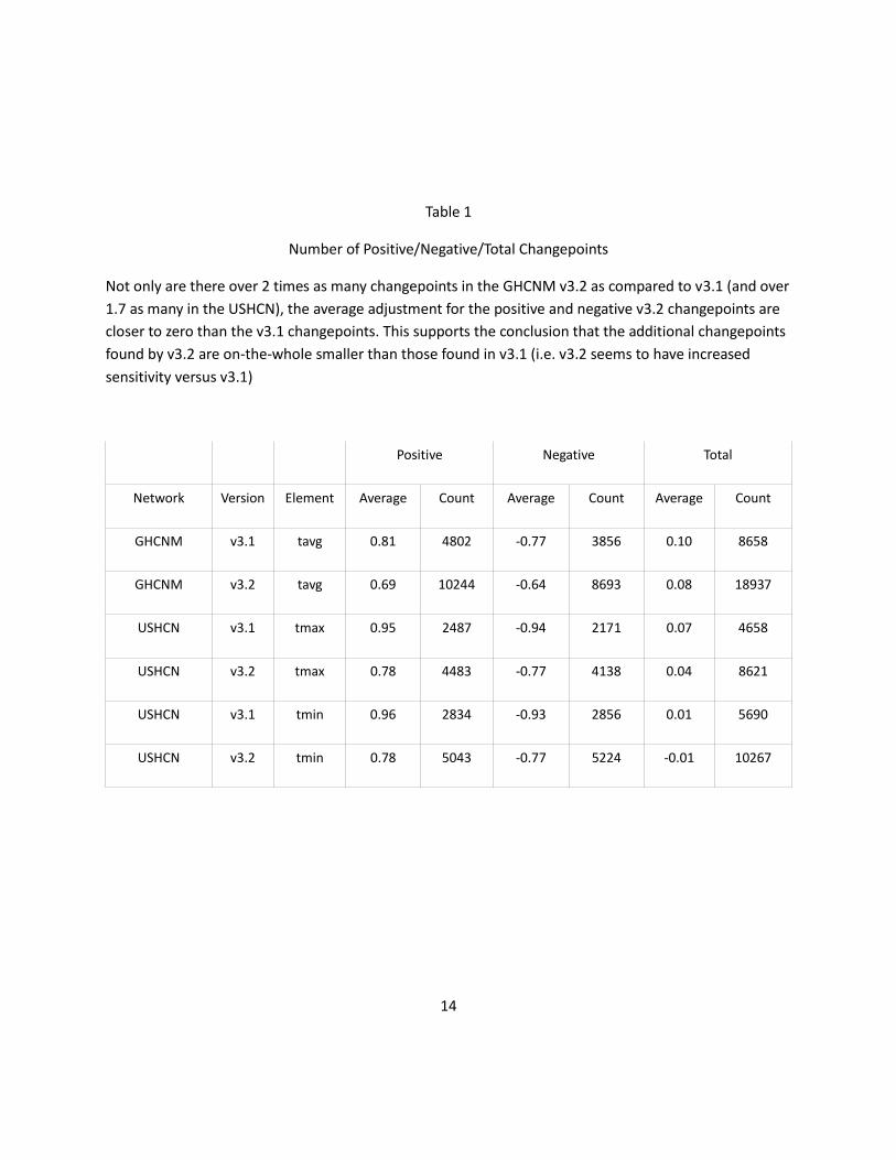
Table 1

Number of Positive/Negative/Total Changepoints

Not only are there over 2 times as many changepoints in the GHCNM v3.2 as compared to v3.1 (and over

1.7 as many in the USHCN), the average adjustment for the positive and negative v3.2 changepoints are

closer to zero than the v3.1 changepoints. This supports the conclusion that the additional changepoints

found by v3.2 are on-the-whole smaller than those found in v3.1 (i.e. v3.2 seems to have increased

sensitivity versus v3.1)

Positive Negative Total

Network Version Element Average Count Average Count Average Count

GHCNM v3.1 tavg 0.81 4802 -0.77 3856 0.10 8658

GHCNM v3.2 tavg 0.69 10244 -0.64 8693 0.08 18937

USHCN v3.1 tmax 0.95 2487 -0.94 2171 0.07 4658

USHCN v3.2 tmax 0.78 4483 -0.77 4138 0.04 8621

USHCN v3.1 tmin 0.96 2834 -0.93 2856 0.01 5690

USHCN v3.2 tmin 0.78 5043 -0.77 5224 -0.01 10267

15

Figure 1a. Histogram of magnitude of bias corrections for all GHCN-M stations outside the

contiguous U.S. (xCONUS) after application of the software changes described in sections 2 and

3. Blue: Version 3.1.0. Red: v3.2.0. Note that although bias adjustments are applied to maximum

and minimum temperature separately for USHCN stations, mean temperature data are adjusted

for all other stations.

16

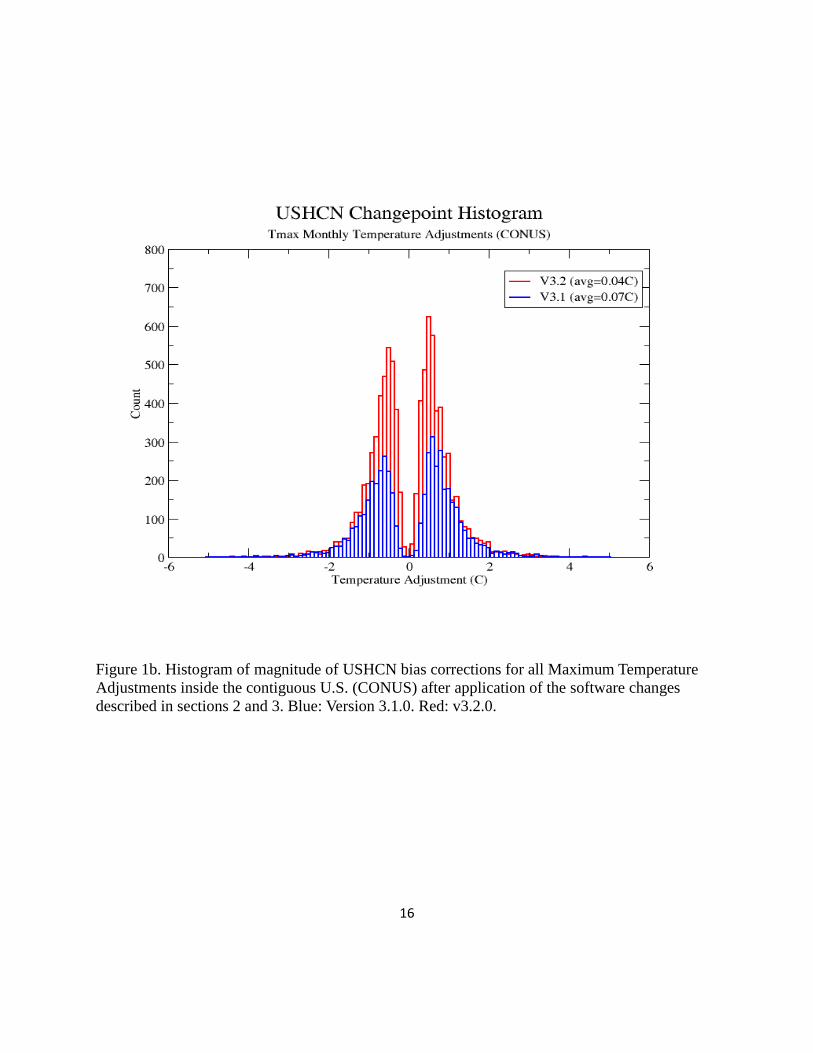
Figure 1b. Histogram of magnitude of USHCN bias corrections for all Maximum Temperature

Adjustments inside the contiguous U.S. (CONUS) after application of the software changes

described in sections 2 and 3. Blue: Version 3.1.0. Red: v3.2.0.

17

Figure 1c. Histogram of magnitude of USHCN bias corrections for all Minimum Temperature

Adjustments inside the contiguous U.S. (CONUS) after application of the software changes

described in sections 2 and 3. Blue: Version 3.1.0. Red: v3.2.0.

18

Figure 2. Percent of (a) global stations (excluding U.S.) and (b) U.S. stations on an annual basis

for which bias adjustments were applied. Dashed: Version 3.1.0. Solid: Version 3.2.0. Note that

bias adjustments are applied to maximum (red) and minimum temperature (blue) for USHCN

stations, and mean temperature data are adjusted for all other stations.

19

Figure 3a. Global land surface annual mean temperature anomalies from 1880 to 2011, before

and after application of software changes. Orig is version 3.1.0 and Base2 includes modifications

to add debugging options and initialization counters. The difference time series also is shown.

Figure 3b. Global land surface annual mean temperature anomalies from 1880 to 2011, with

Base2 and Base2c modifications (changes to address asynchronous execution problems). The

difference time series also is shown.

20

Figure 3c. Global land surface annual mean temperature anomalies from 1880 to 2011, with

Base2c and Roth1 modifications (Kendall-Thiel Paired-slope function x-axis median). The

difference time series also is shown.

Figure 3d. Global land surface annual mean temperature anomalies from 1880 to 2011, with

Roth1 and Roth2 modifications (Semi-hierarchical Segmentation function “corner case”). The

difference time series also is shown.

21

Figure 3e. Global land surface annual mean temperature anomalies from 1880 to 2011, with

Roth2 and Roth3 modifications (Kendall-Thiel Paired-slope function looping index). The

difference time series also is shown.

Figure 3f. Global land surface annual mean temperature anomalies from 1880 to 2011, with

Roth3 and Roth4 modifications (Kendall-Thiel Paired-slope function incorrectly assumed no

missing data in array.). The difference time series also is shown.

22

Figure 3g. Global land surface annual mean temperature anomalies from 1880 to 2011, with

Roth4 and Roth5 modifications (Standard Normal Homogeneity Test (SNHT) array index of the

last observation). The difference time series also is shown.

Figure 3h. Global land surface annual mean temperature anomalies from 1880 to 2011, with

Roth5 and Roth6 modifications (BIC Sloped vs. TPR0 data model test index for last

observation). The difference time series also is shown.

23

Figure 4. Global annual average land surface temperature anomalies for v3.1.0 (blue), v3.2.0

(red), and the difference between the two (solid black) over the period 1880 to 2011.

24

Figure 5. Map of 5X5 grid box annual temperature trends (1901-2011) for (a) v3.1.0, (b) v3.2.0,

and (c) the difference between v3.2.0 and v3.1.0. Grid boxes with data in at least 70% of the

years between 1901 and 2011 are shown.

25

Figure 6. Map of 5X5 grid box annual temperature trends (1951-2011) for (a) v3.1.0, (b) v3.2.0,

and (c) the difference between v3.2.0 and v3.1.0. Grid boxes with data in at least 70% of the

years between 1951 and 2011 are shown. Stations within the grid boxes encompassed by a red

circle in Figure 6c are shown in Figure 7 below.

26

70N-75N, 65W-70W

ID: 40371090000 70.5N 68.5W CLYDE,N.W.T.,Canada

Grid box contains only one station.

25N-30N, 75W-80W

ID: 42378073000 25.1N 77.5W NASSAU AIRPORT, Nassau

Contains one other station – 30 year period of record from 1965 to 1995

27

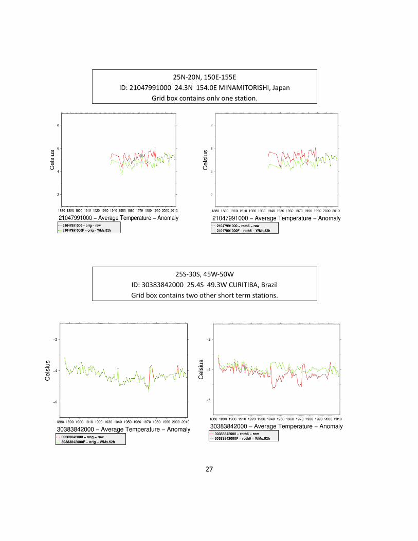
25N-20N, 150E-155E

ID: 21047991000 24.3N 154.0E MINAMITORISHI, Japan

Grid box contains only one station.

25S-30S, 45W-50W

ID: 30383842000 25.4S 49.3W CURITIBA, Brazil

Grid box contains two other short term stations.

28

Figure 7. Examples of individual station series with large changes in trend between v3.1.0 and

v3.2.0. The location of each grid box is denoted by a red circle in Figure 6c. The unadjusted

difference series (red) and bias adjusted difference series (green) are shown. These are annual

average anomaly plots with the average of the surrounding network removed to indicate the

station's stability with the underlying local climate.

20S-25S, 130E-135E

ID: 50194326000 23.8S 133.8E ALICE SPRINGS, Australia

Grid box contains three other short term stations.