Modification of kinetic theory for frictional spheres part I

Yang, L.; Padding, J.T.; Kuipers, J.A.M.

Published in:Chemical Engineering Science

DOI:10.1016/j.ces.2016.05.031

Published: 02/10/2016

Document VersionAccepted manuscript including changes made at the peer-review stage

Please check the document version of this publication:

• A submitted manuscript is the author's version of the article upon submission and before peer-review. There can be important differencesbetween the submitted version and the official published version of record. People interested in the research are advised to contact theauthor for the final version of the publication, or visit the DOI to the publisher's website.• The final author version and the galley proof are versions of the publication after peer review.• The final published version features the final layout of the paper including the volume, issue and page numbers.

Link to publication

General rightsCopyright and moral rights for the publications made accessible in the public portal are retained by the authors and/or other copyright ownersand it is a condition of accessing publications that users recognise and abide by the legal requirements associated with these rights.

• Users may download and print one copy of any publication from the public portal for the purpose of private study or research. • You may not further distribute the material or use it for any profit-making activity or commercial gain • You may freely distribute the URL identifying the publication in the public portal ?

Take down policyIf you believe that this document breaches copyright please contact us providing details, and we will remove access to the work immediatelyand investigate your claim.

Download date: 17. Aug. 2018

1

Modification of Kinetic Theory for Frictional Spheres, Part I: Two-fluid model derivation and numerical implementation

L. (Lei) Yang, J.T. (Johan) Padding*, J.A.M. (Hans) Kuipers Department of Chemical Engineering and Chemistry, Eindhoven University of Technology, 5600

MB, Eindhoven, The Netherlands Corresponding author’s e-mail: J.T.Padding@tue.nl

Keywords: Fluidized granular bed; Rough particles; Rotation; Two-fluid model; Kinetic Theory

ABSTRACT

We derive a kinetic theory of granular flow (KTGF) for frictional spheres in dense systems, including rotation, sliding and sticking collisions. We use the Chapman-Enskog solution procedure of successive approximations, where the single-particle velocity distribution is assumed to be nearly Maxwellian both translationally and rotationally, as assumed by McCoy et al. (1966). An expression for the first-order particle velocity distribution function is derived, which includes the effects of particle rotation and friction. Using a simple moment method, balance equations for mass, momentum and energy are derived with closure equations for viscosities, and thermal conductivities and collisional energy dissipation rates of angular and translational kinetic energy. Because the internal angular momentum changes are coupled to the flow field, the stress tensor contains anti-symmetric components which are associated with a rotational viscosity. In the resulting closure equations, the rheological properties of the particles are explicitly described in terms of the friction coefficient. The model has been incorporated into our in-house two-fluid model (TFM) code for the modeling of dense gas-solid fluidized beds. For verification, a comparison of the present model in the limit of zero friction with the original (frictionless) KTGF model is carried out. Simulation results of both models agree well. In the next part, simulation results obtained with the new model will be compared with experimental data and discrete particle model (DPM) simulations. 1. Introduction

Gas-solid fluidized beds find a widespread application in processes involving combustion, separation, classification, and catalytic cracking (Davidson et al., 1985; Kunii and Levenspiel, 1991). Understanding the dynamics of fluidized beds is a key issue in improving efficiency, reliability and scale-up. Owning to enormous increase in computer power and algorithm development, fundamental modelling of multiphase reactors has become an effective tool. For larger scale applications, the Euler-Euler approach (Kuipers et al., 1992, Gidaspow, 1994, Lu and Gidaspow, 2003, Lu et al., 2003) is considered to be the most effective. The so-called two-fluid model (TFM) has emerged as a very promising tool as a result of its compromise between computational cost and amount of detail provided. In TFM, both the gas phase and the solid phase are treated as fully interpenetrating continua and are described by separate governing balance equations of mass and momentum. The challenge of the model is to establish an accurate hydrodynamic and rheological description of the solid phase. State-of-the-art closures have been obtained from the kinetic theory of granular flow, initiated by Jenkins & Savage (1983), Lun et al. (1984), Jenkins & Richman (1985), Lun & Savage (1987), Ding & Gidaspow (1990), Lun et al. (1991), and Nieuwland (1995). This theory is based on the classical kinetic theory of dense gases (Chapman and Cowling, 1970).

The original KTGF models of Jenkins and Savage (1983), Lun et al. (1984), Jenkins and Richman (1985) and Gidaspow (1994) are derived for frictionless and nearly elastic particles with translational motion only. Various extension have been proposed. For example, Sun et al. (2009) presented a KTGF with anisotropic second-order velocity moments for inelastic and frictionless particles. An extra model for the third-order velocity moment was used to close the equations for the second-order velocity moments. With this they predicted that in a fluidized bed the simulated second-

2

order moment in the vertical direction is 1.1 to 2.5 (or even 4 for small particles) times larger than the second moment in the lateral direction. It was found that the relatively large anisotropy values always occurred at sufficiently dilute conditions. Similarly, Chen et al. (2012) found obvious anisotropy in the second moments in dilute riser flow. In dense gas-solid fluidized beds the anisotropy in the second velocity moments is much weaker however. In the present work we focus on applications in dense gas-solid fluidized beds. We will therefore assume that the second moments can be described by an isotropic granular temperature combined with relatively small deviations which are controlled, as we will show in this paper, by gradients in the average velocity field.

As mentioned above, most KTGF models focus on frictionless particles. In reality, however, granular materials are frictional. The roughness of the granular materials has been shown to have a significant effect on stresses at least in the quasi-static regime (Sun & Sundaresan, 2011). After a binary collision between rough particles, the particles can rotate due to surface friction. Thus, translational kinetic energy may exchange with rotational kinetic energy. Attempts to quantify the friction effect have been somewhat limited. Lun and Jenkins (1987) developed a kinetic theory for a system of inelastic, rough spherical particles to study the effects of particle surface friction and rotational inertia. Two collisional parameters were used. One was the normal restitution coefficient and the other was the roughness coefficient to characterize the effects of surface friction. In their theory only dense systems, where the major stress contribution arises from particle collisions, was considered. However, at low solids concentrations the kinetic stress contribution becomes dominant. Lun (1991) extended the kinetic theory to be appropriate for both dilute and dense granular flows including kinetic as well as collisional contributions for stresses and energy fluxes. Translational and rotational granular temperatures were involved to characterize the kinetic fluctuation energies. An extra energy balance equation for the rotational granular temperature was derived. Goldshtein and Shapiro (1995) developed a kinetic theory for rough inelastic spheres combining the translational and rotational granular temperatures into a total granular temperature. Their theory has been improved by Wang et al. (2012a, 2012b) to develop kinetic theory for granular flow of rough spheres. Chou and Richman (1998) derived a theory for homogeneous shear flows of identical, smooth and highly inelastic spheres in which the solids volume fraction, mean velocity and each component of the full second moment of fluctuation velocity were treated as mean fields. The constitutive relation for the granular flow of smooth, inelastic, spherical particles was derived by Kumaran (2004) in the adiabatic limit where the length scale for the conduction of energy is small compared to the macroscopic scale. Later, Kumaran (2006) developed constitutive relations for the granular flow of rough spheres in the limit where the energy dissipation in a collision is small compared to the energy of a particle. He also pointed out the antisymmetric component in the stress tensor for rough and partially rough particles. However, these models didn’t account for the dependence on the friction coefficient explicitly.

Abu-Zaid and Ahmadi (1990) introduced the friction coefficient into the kinetic theory model to include the effects of frictional energy dissipation during collision explicitly. But they made the assumption that the particles were sufficiently small such that the effects of particle-spin could be neglected. Jenkins and Zhang (2002) derived a simple kinetic theory for collisional flows of identical, slightly frictional, nearly elastic spheres. An effective restitution coefficient which was given in terms of the collision parameters, namely normal coefficient of restitution e, friction coefficient μ, and tangential coefficient of restitution β. However, a comparison between experiment and simulation by Goldschmit et al. (2001) for an effective restitution coefficient of 0.73 showed that the simulated bubble dynamics was too vigorous, which indicated that the effects of particle friction could not be replaced by using an effective (smaller) restitution coefficient.

Rau and Nott (2008) derived a kinetic theory for rough inelastic particles. They used a simple hard sphere collision model with two restitution coefficients, namely the normal restitution coefficient e ( 0 1e≤ ≤ ) and the tangential restitution coefficient β ( 1 1β− ≤ ≤ ). In effect, therefore, their theory applies to infinitely high friction coefficient. However, in fluidized beds the particles mostly undergo sliding contacts. Thus, for the study of hydrodynamics in fluidized beds, inclusion of the friction coefficient is important because distinguishing between sliding and sticking collisions is necessary. Using detailed simulations, Rau and Nott (2008) determined velocity distribution functions for both nearly perfectly rough and nearly perfectly smooth particles. As expected, in case of nearly perfectly

3

rough particles, the mean spin was found to be equal to half the macroscopic rotation rate of the particle velocity field, while in case of nearly perfectly smooth spheres, the mean spin could be any value. Based on the measured velocity distribution functions, they derived different closures equations. However, in their velocity distribution function, they neglect the coupling between rotation and translation (last term of our Eq. (2.22)).

Recently, Zhao et al. (2013) developed a kinetic theory model for rough spheres. Both particle friction and rotation were considered for energy fluxes. However, they did not derive the expression for the first-order particle velocity distribution function and the effect of rotation on the particle velocity distribution function was not included. In the Hermite polynomials proposed by Grad (1949) to write the velocity distribution function, the coefficients given by Enwald et al. (1996) were used without considering the particle friction. Sun and Sundaresan (2013) proposed a new expression for the radial distribution function at contact as well as modifications to the Garzó-Dufty (GD) KT model (1999) expressions for shear stress and energy dissipation rate through data obtained from discrete element method (DEM) simulations. Their model relied on empiricism, particularly in the corrections for the shear stress. According to their simulation, the granular temperature in the dilute region (solids volume fraction < 0.2) was overestimated due to neglect of the rotational degrees of freedom.

The present work is concerned with further development of a kinetic theory for rough spheres including particle friction and rotation. We focus on the inertial regime (Chialvo et al., 2012) so that kinetic theory can be applied without corrections for the drag caused by the interstitial fluid. Following Kumaran (2006), an antisymmetric contribution due to the convective transport of rotational momentum is incorporated in the solid stress tensor. The present model is first incorporated into our in-house Euler-Euler code. Simulations of gas-solid fluidized bed are carried out. Comparison between the present model and the original model is then made. Finally, we use the present model to investigate the influence of particle surface friction for inelastic particles. In this first part, we focus on the derivation of the model and verification of model implementation in well-known limits. In the next part, we will compare results from the present model with those obtained from a Discrete Particle Model.

2. Kinetic theory of rough spheres

2.1 Binary collisions

1

2

k

t

G

θ

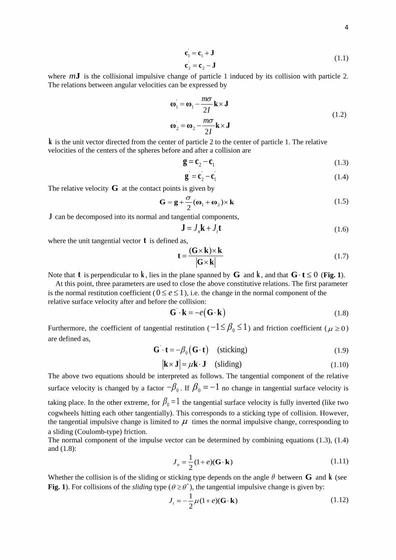
Fig. 1. Sketch of a binary collision between frictional spheres.

We start the analysis by considering an inelastic collision between two frictional spheres (Fig. 1). It is assumed that the interaction forces are impulsive and therefore all other finite forces are negligible during a collision. In this work, we will mainly adopt the notation used by Walton (1992) and Foerster et al. (1994). The spheres have mass m, diameter σ, and moment of inertia I around their respective

centers. The balance of linear momentum requires that the velocities 1c and 2c of the two spheres

before collision and the velocities ' '1 2, c c after collision have the relation

4

'1 1'2 2

= +

= −

c c Jc c J

(1.1)

where mJ is the collisional impulsive change of particle 1 induced by its collision with particle 2. The relations between angular velocities can be expressed by

'1 1

'2 2

2

2

mI

mI

σ

σ

= − ×

= − ×

ω ω k J

ω ω k J (1.2)

k is the unit vector directed from the center of particle 2 to the center of particle 1. The relative velocities of the centers of the spheres before and after a collision are

2 1= −g c c (1.3) ' ' '

2 1= −g c c (1.4) The relative velocity G at the contact points is given by

1 2( )2σ

= + + ×G g ω ω k (1.5)

J can be decomposed into its normal and tangential components,

n tJ J= +J k t (1.6) where the unit tangential vector t is defined as,

( )× ×=

×G k kt

G k (1.7)

Note that t is perpendicular to k , lies in the plane spanned by G and k , and that 0⋅ ≤G t (Fig. 1). At this point, three parameters are used to close the above constitutive relations. The first parameter

is the normal restitution coefficient ( 0 1e≤ ≤ ), i.e. the change in the normal component of the relative surface velocity after and before the collision:

( )' e⋅ = − ⋅G k G k (1.8)

Furthermore, the coefficient of tangential restitution ( 01 1β− ≤ ≤ ) and friction coefficient ( 0µ ≥ ) are defined as,

( )'0 (sticking)β⋅ = − ⋅G t G t (1.9)

(sliding)µ× = ⋅k J k J (1.10) The above two equations should be interpreted as follows. The tangential component of the relative

surface velocity is changed by a factor 0β− . If 0 1β = − no change in tangential surface velocity is

taking place. In the other extreme, for 0 1β = the tangential surface velocity is fully inverted (like two cogwheels hitting each other tangentially). This corresponds to a sticking type of collision. However, the tangential impulsive change is limited to µ times the normal impulsive change, corresponding to a sliding (Coulomb-type) friction. The normal component of the impulse vector can be determined by combining equations (1.3), (1.4) and (1.8):

1 (1 )( )2nJ e= + ⋅G k

(1.11)

Whether the collision is of the sliding or sticking type depends on the angle θ between G and k (see Fig. 1). For collisions of the sliding type ( *θ θ≥ ), the tangential impulsive change is given by:

1 (1 )( )2tJ eµ= − + ⋅G k (1.12)

5

For sticking collisions ( *θ θ≥ ), the tangential impulsive change is given by:

( ) ( )02

12 1 4tJ

m Iβσ

+= ⋅

+G t

(1.13)

When *θ θ= , the above two expressions of tangential impulse must agree, so using cosG θ⋅ =G k and sinG θ⋅ = −G t , we find

2*

0 1 (1 )(1 )cot4

meI

σβ µ θ= − + + +

(1.14)

Thus the critical angle is determined by

2

*

0

1tan (1 )1 4

e mI

σθ µβ

+= +

+ (1.15)

For homogenous spheres 2

10mI σ

= , and thus:

*0

0

7 1tan2 1

eθ µ µβ

+= =

+ (1.16)

2.2 Transport equations and collisional production

The goal of any kinetic theory of granular flow is to obtain the transport balance equations for relevant hydrodynamic moments (e.g. mass-, momentum- and energy-density), along with closures for the transport properties such as shear viscosity and (pseudo-)thermal conductivity. In the following we will derive the Boltzmann equation for the probability distribution function of finding a particle at a specific location with a specific translational and rotational velocity. By taking ensemble averages we can then derive the corresponding Maxwell transport equations. Following Grad (1949), we assume that the state of the system can be described accurately by an extended, but limited, set of moments of the velocities and angular velocities. The balance equations for Nth order moments do not form a closed system, because they generally contain fluxes and production terms which may involve moments of order (N+1). Therefore, also following Grad (1949), we will construct a first approximation to the probability distribution function by expanding the unperturbed probability distribution function (which is a simple Maxwellian) into Hermite polynomials. The Hermite expansion coefficients are then determined self-consistently, such that the first approximation of the probability distribution functions reproduces the expected moments. The system is closed because we consider as many Hermite coefficients are there are moments. Once the first approximation to the probability distribution function is known, we can compute fluxes and production terms for each of the hydrodynamic moments. We denote the single-particle probability distribution function to encounter a particle at position r with instantaneous velocity c and angular velocity ω at time t by ( , , , )f f t= r c ω . With this

definition, the number of particles per unit volume n can be obtained from d dn f= ∫∫ c ω , and the

mean (ensemble average) value of a quantity ψ is defined as:

d dn fψ ψ= ∫∫ c ω (2.1) Here, as in McCoy et al. (1966), we assume the unperturbed (zeroth-order) probability distribution function is of Maxwellian form for both the translational and rotational velocity fluctuations:

( )

3 2 3 2 2 2(0) 1 1 Ω, , , exp

2 2 2t r t r

I C If t nm mπ π

= − + Θ Θ Θ Θ

r c ω

(2.2)

Here C ( = −C c v ) and Ω ( = −Ω ω ω ) are the peculiar translational and rotational velocities, defined relative to the local average particle velocity v and average angular velocity ω . The

6

translational and rotational granular temperatures are a measure for the mean square peculiar velocities. More precisely they are given by 2 3t CΘ ≡ and 2 3r I mΘ ≡ Ω . In deriving the Boltzmann equation it is assumed that only binary encounters are important. Based on Chapman & Cowling (1970), we consider a particle with external force mF and external torque IT , which may be a function of r and t (note that F and T are therefore the acceleration and angular acceleration, respectively, due to external forces and torques). For particles in fluidized beds, the dominant external forces and torques include gravity forces and fluid-particle interactions such as buoyancy, drag and lift. Between times t and t+dt, the velocities c , ω of any particle that does not collide with another will change to dt+c F , dt+ω T and its position vector r will change to

dt+r c . There are ( , , , )d d df tc ω r c r ω particles at time t. After time interval dt, there are ( d , d , d , d )d d df t t t t t+ + + +c F ω T r c c r ω particles. The number of particles in the second set

differs from the first one. The net gain of particles to the second set must be proportional to

d d d dtc ω r , and will be denoted by d d d de f tt

∂∂

c ω r . On dividing by d d d dtc ω r and making dt tend

to zero, Boltzmann’s equation for f is obtained, e ff f f f

t t∂∂ ∂ ∂ ∂

⋅ + ⋅ + ⋅ + =∂ ∂ ∂ ∂ ∂

F T cc ω r

(2.3)

The quantity e ft

∂∂

is equal to the rate of change, owing to collisional encounters, in the velocity

distribution function f at a fixed point. Multiplying Boltzmann’s equation with a local property ( ), ,ψ c ω r , which may depend on the particle velocity, angular velocity and/or position, and changing independent variables to the peculiar velocities C , Ω instead of absolute velocities c , ω , we find after several transformations (similar to Chapman & Cowling, 1970, p48) the Maxwell transport equations:

( )

( )

( ) i ii i i j j

i i j i i

iij j

i i i j

D Dv vn nC n F n CDt r Dt C r C C

Dn n CDt r

ψ ψ ψ ψθ ψ ψ θ

ω ψ ψ ψ ωθ χ ψ

∂∂ ∂ ∂ ∂ + + − − + + ∂ ∂ ∂ ∂ ∂ ∂ ∂ ∂ ∂

+ + + = ∂Ω ∂Ω ∂Ω ∂

(2.4)

where for clarity the Einstein summation convention is used, i.e. a sum over all components (x, y, and z) is implied whenever the same component index (i or j) appears twice in a product. The rate of

change e ft

∂∂

due to collisions can be written as follows according to Lun et al. (1984) and Lun (1991),

d d ( ) ( )ec c

ft

ψ θ ψ χ ψ∂= −∇ ⋅ +

∂∫∫ c ω (2.5)

where the collisional flux term is: 3

' (2)1 1 1 1

0

( ) ( ) ( , , , , , )d d d d d2c fσθ ψ ψ ψ σ

⋅ >

= − − ⋅ +∫G k

G kk r k c ω r c ω k c ω c ω (2.6)

and the collisional source term is: 2

' ' (2)1 1 1 1 1 1

0

( ) ( ) ( , , , , , )d d d d d2c fσχ ψ ψ ψ ψ ψ σ

⋅ >

= + − − ⋅ +∫G k

G k r k c ω r c ω k c ω c ω (2.7)

Note that the tensorial rank of the collisional flux term is one higher than that of ψ and the tensorial rank of the collisional source term is equal to that of ψ . As usual, we will assume that the 2-particle

distribution function (2)f factorizes as a product of two single-particle distribution functions, with

position correlations included through the radial distribution function. Following a Taylor series gives

the following expression for the 2-particle distribution function (2)1 1( , , , , , , )f tσ+r k c ω r c ω :

7

(2)1 1 0 1 1 1

0 1 11

1( , , , , , , ) ( , , ) ( , , , ) ( , , , )2

1 ln2

f t g f t f t

fg f f fff

σ σ σ

σ

+ = + +

= ⋅ + ⋅∇

r k c ω r c ω r k c ω r k c ω r c ω

k (2.8)

where 0g is the radial distribution function at contact.

2.3 Balance laws

For convenience, in writing the balance laws corresponding to the higher moments of velocity fluctuation we adopt the following definitions,

1 2 1 2

1 2 1 2

1 2 1 2

1 2 1 2

... ... ;

... ... ;

... ( ... );

... ( ... );

n n

n n

n n

n n

i i i i i i

i i i i i i

i i i i i i

ji i i j i i i

M C C C

N

mC C C

mC C C

χ χ

θ θ

≡

≡ Ω Ω Ω

≡

≡

(2.9a-9d)

Different balance equations can be obtained by inserting different properties ψ in equation (2.4). (1) Let ψ be m ,

( ) 0i

i

vD nm nmDt r

∂+ =

∂ (2.10)

which is the familiar continuity equation (mass conservation).

(2) Let ψ be imC ,

( )iji ij i

j

Dv M FDt r

ρ θ ρ ρ∂+ + =

∂ (2.11)

Here, ij ji ijP Mθ ρ= + is the total pressure tensor (negative of the stress tensor). This is the Navier-

Stokes equation for the average particle momentum. We note that for smooth spheres ji ijθ θ= . However, for rough spheres this is not the case, i.e. the pressure tensor contains asymmetric components. We will return to this point later.

(3) Let ψ be iIΩ ,

( ) ( )( )ij i i

j

DnI I IDt rω θ χ∂

+ Ω = Ω∂

(2.12)

A collisional source term appears because the sum of angular momenta (around the respective sphere’s center of mass) is not conserved in binary collisions. Similar to Lun et al. (1991), the collisional angular momentum flux ( )j iIθ Ω is found to be zero.

(4) Let ψ be i imC C , using the definition of granular temperature, the energy balance equation can be written as,

( ) ( )3 1 12 2 2

jtjii jii kj i i

j k

vD M P mC CDt r r

ρ θ ρ χ∂Θ ∂

+ + + =∂ ∂

(2.13)

Here jiiMρ is the transported (kinetic) part of the energy flux vector, and jiiθ is the collisional part.

(5) Let ψ be i iIΩ Ω , the energy balance equation for rotational granular temperature can be written as,

8

( ) ( ) ( )3 1 1( ) ( )2 2 2

jrj i i j i i j k k j i i

j k

D I nIC nI C I IDt r r

ωρ θ θ χΘ ∂ ∂+ Ω Ω + Ω Ω + Ω + Ω = Ω Ω

∂ ∂

(2.14) We note that according to our calculations terms like j i inIC Ω Ω , j knI CΩ and ( )k jIθ Ω vanish. Besides, in this work we will assume that in the bulk of the system the mean rotational velocity is so small that we can set it to zero, in which case the production term due to gradients in the mean rotational velocity (last term on the left hand) side vanishes. So we do not have a production term for rotational granular temperature in the present theory. This is in contrast with the work of Rao and Nott (2008), who kept the production term due to the existence of a mean rotational velocity. Note that we do still have a collisional source/sink term on the right hand side. (6) Let ψ be i jmC C , the balance law for the mean of the second moment of velocity fluctuation is

derived by deducting the energy equation (2.13).

( ), ( ), ,1 1 1 1( )2 3 3 2

ijkij ij kpp k n j i n km m k ij i j

D M Q Q P v P v mC CDt

ρ δ δ χ∧

∧

+ − + − = (2.15)

where we defined 1 ( )2kij kij kijQ Mθ ρ= + . Here and in the following a comma denotes differentiation

with respect to a spatial coordinate, e.g. ,i j ij

a ax∂

=∂

, round brackets around paired indices denotes

symmetric averaging over all permutations of the indices, e.g. ( )( )12i j i j j ia b a b a b= + and

( )( )16i jk i jk i kj j ik j ki k ij k jia b a b a b a b a b a b a b= + + + + + , and the traceless part of a second-rank tensor

is denoted by a hat above its symbol, e.g. ( ) ( ) ( )13i j i j k k ijmC C mC C mC Cχ χ χ δ

∧

= − . Note that Eq.

(2.15) describes the evolution of the anisotropic part of the second moment of velocity fluctuations; the evolution of the isotropic part, which is the granular temperature, is given by Eq. (2.13). (7) Let ψ be i jIΩ Ω , similarly, after deducing the angular energy equation (2.14), the second

moment of angular velocity fluctuation is,

( ) ( )), ,(

1 1 1( ) ( ( ) )2 2 3

1 1( )3 2

ijk i j k i j ij k p p k p p

k

i k p kk j ij p k k p i j

D N I nIC I nICDt r

P nI C I I

ρ θ δ θ

ω δ θ ω χ

∧

∧

∂ + Ω Ω + Ω Ω − Ω Ω + Ω Ω ∂

+ − Ω + Ω = Ω Ω

(2.16)

(8) Let ψ be i j kmC C C , the expression for the third moment of velocity fluctuation can be written as,

( ), ( ) ( ),2 3 6ijklijk l n i jk m ij k m i j k

n

DMQ P M Q u mC C C

Dt rρ χ∂

+ − + =∂

(2.17)

where we defined 1 ( )2lijk lijk lijkQ Mθ ρ= + .

(9) Let ψ be i j kI CΩ Ω , by using the linear moment balance law, the mixed third moment of angular and translational velocity fluctuations can be expressed as,

9

( ) ( )

( ) ( ) ( )

( )

2

i j kn i j k ij kn i j k n kn i j mn nm

n m

nnkn i j m kn m i j in m j k i j k

m m

D CnI I C nI C C I M

Dt r m r

v n I C I I C I Cr r

θ δ δ δ θ ρ

ωδ δ θ δ θ χ

Ω Ω ∂ ∂+ Ω Ω + Ω Ω − Ω Ω +

∂ ∂

∂ ∂+ Ω Ω + Ω Ω + Ω = Ω Ω

∂ ∂(2.18)

2.4 Second approximation for (1) ( , , , )f tr c ω and linear theory

The balance laws apply to averaged quantities ψ , and therefore depend on our assumption about the single particle distribution function f. Although in homogeneous systems it is reasonable to assume, to first order, a Maxwellian form, the distribution function is expected to alter under the influence of (relatively small) gradients in the average velocity, average angular velocity, translational granular temperature and rotational granular temperature fields. We therefore need a method to estimate these deviations. Following Grad (1949), we write the second approximation to the single particle distribution function with rotation as a Hermite polynomial series:

'2 2 2 3

(1) (0)3 3 3

12! 2! 2! 3!

( , , , ) ( , , , )...

2! 3! 2!

ij ij ij ijki i

i i i j i j i j i j k

ijk ijk ijk

i j k i j k i j k

a b b aa b

c c c c c c cf t f t

c d bc c c

∂ ∂ ∂ ∂ ∂ ∂− − + + + − ∂ ∂Ω ∂ ∂ ∂Ω ∂Ω ∂ ∂Ω ∂ ∂ ∂ = ∂ ∂ ∂ − − − + ∂ ∂ ∂Ω ∂Ω ∂Ω ∂Ω ∂ ∂Ω ∂Ω

r c ω r c ω

(2.19)

where (0) ( , , , )f tr c ω is the (zeroth order) Maxwellian distribution function, eq. (2.2). The

coefficients ', , , , , ...i ij ijk ij ij ijka a a b b b , to be determined next, may depend on r and t but crucially

do not depend on c and ω . If the mean values of velocity fluctuations iC , iΩ , i jC C , i jΩ Ω ,

i jC Ω , i j kC C Ω , i j kC Ω Ω based on the second approximation (1)f are carried out, it can be

found that ' 0i i ij ij ijk ijka b b b c d= = = = = = , 0ii iia b= = . Also

2( ) ( )3 6

ij t ij ij

ijk ijk

ijkp t ij kp t ij kp ijkp

ijk i j k

t r rij kn kn ij ijkn i j k n

M aM a

M a a

b C

m ma b C CI I

δ

δ δ δ

δ δ δ

= Θ +

=

= Θ + Θ +

= Ω Ω

Θ Θ Θ+ + = Ω Ω

(2.20a-20e)

Based on Jenkins & Richman (1985), we derive the following expressions for coefficients ijka and ijkb

1 ( )513

ijk imm jk jmm ik kmm ij

ijk imm jk

a a a a

b b

δ δ δ

δ

= + +

= (2.21a-21b)

Because , ijk ijka b have no direct physical interpretation, we focus on , imm imma b , which are directly related to the energy flux vectors. As a result, the second approximation for the distribution function can be expressed as

10

2 2(1) (0)

2 2( , , , ) 1 ( 5) ( 3) ( , , , )2 10 6

ij imm immi j i i

t t t t r r

a a IbC If t C C C C f tm m

Ω= + + − + − Θ Θ Θ Θ Θ Θ

r c ω r c ω

(2.22) Inserting equations (2.20a-2.20e) into the second and third moment balances, respectively, the second moment (2.15) may be rewritten in terms of , ij imma a

( ) ( )

1 2( ) ( ) ( ) 25 3

2 1( ) ( ) ( ) ( )3 3

13

ijijimm jmm kmm ij t

j i k

ji mkj kj ki ki km km ij kij ij kpp

k k k k

i j k k ij

Daa a a D

Dt r r r

vv va a ar r r r

mC C mC C

ρ ρ ρ ρ δ ρ

θ ρ θ ρ θ ρ δ θ δ θ

χ χ δ

∧ ∂ ∂ ∂+ + − + Θ ∂ ∂ ∂

∂ ∂ ∂ ∂+ + + + − + + − ∂ ∂ ∂ ∂

= −

(2.23)

where 123

jiij

j i

vvDr r

∧ ∂∂= + − ∇ ⋅

∂ ∂v is the traceless and symmetric rate of strain tensor.

For the third moment balance equation (2.17), let j=k, ( 0ijkpa = ) and insert the expressions for

ijM , ijkM , ijknM in equations (2.20a-2.20c) to obtain

( ) ( )

( )

2( )5 7 (5 2 )

1 7 2 2 25

ikk tlikk t li t ni ni nk t nk nk

i l l n

i m k i kknn inn knn mkk mik i k k

k m i m m

Da a a aDt r r r r

v v v v va a a mC C Cr r r r r

ρρ θ ρ δ θ ρ δ ρ

ρ θ θ χ

∂ Θ ∂ ∂ ∂+ + + Θ − Θ + + Θ +

∂ ∂ ∂ ∂

∂ ∂ ∂ ∂ ∂+ + + + + = ∂ ∂ ∂ ∂ ∂

(2.24) For the angular third moment (2.18), using equation (2.20c-2.20e),

( ) ( )

( ) ( ) ( )

( ) ( )

2

jjkn j j k kn t r kn r kn r mn t mn mn

n m

nnkn jjm m j j m in j k j j k

m m

DbnI I C a a

Dt r r

v nIb I I C I Cr r

θ δ ρ ρ δ θ ρ δ

ωδ θ θ δ χ

∂ ∂+ Ω Ω + Θ Θ + Θ − Θ + Θ +

∂ ∂

∂ ∂+ + Ω Ω + Ω = Ω Ω

∂ ∂

(2.25)

Equations (2.23-25) are used to determine , , , , , , i t r ij ijk ijju a a bρ Θ Θ . Some assumptions

regarding the order of magnitude of the spatial derivatives of the mean fluid field and granular

temperature must be made to obtain a solution. Let L, U, 0Θ be the characteristic values of length, velocity, and granular temperature, and then use these to form dimensionless quantities proportional to the spatial gradients of granular temperature and mean velocity. In order to rewrite the moment

balance equations in dimensionless forms, , , , ij ijk ijja a bρ are divided by typical values

0 (2) (3) (3), , , a a bρ . We also make the assumption that 3 2 3 2(2) 0 (3) 0 (3) 0, , , L a a bσ Θ Θ Θ are

small and of the same order of magnitude. The non-dimensional granular temperature gradient, the

non-dimensional gradient of mean velocity and 0U Θ are all of order one.

Following Jenkins and Richman (1985), the expression for ( ), ( )c cχ θψ ψ are still linear in the perturbation and the spatial gradients of velocity and granular temperatures. The terms quadratic in

ija , ijka and ijkb that appear in the product of (1)1 1( , , )f r c ω with (1)

2 2( , , )f r c ω can be neglected

11

when compared with linear terms, while the products of ija , ijka and ijkb with the spatial gradients of the mean fields will be also ignored. Thus the flux and source terms can be written as,

( ) ( ) ( ) ( ) ( ) ( )c i i ijk ijkp ijkpjk jkp jkpA B B B Ca a bθ ψ ψ ψ ψ ψ ψ= + + + + (2.26)

( ) ( ) ( ) ( ) ( ) ( )c jk jkp jkpjk jkp jkpE F F F Da a bχ ψ ψ ψ ψ ψ ψ= + + + + (2.27)

Using definitions (0)01 1 1( , , , )f f t= r c ω , (0)

02 2 2( , , , )f f t= r c ω , we find for the flux term 3

'001 02 1 1

0

( ) ( ) d d d d d2i iAg f f kσψ ψ ψ

⋅ >

= − − ⋅∫G k

G k k c ω c ω (2.28a)

4'0 02

01 02 1 1010

( ) ( ) ln d d d d d4i iBg ff f k

fσψ ψ ψ

⋅ >

= − − ⋅ ⋅∇∫G k

G k k k c ω c ω (2.28b)

3 2 2'0 02 01

01 02 1 12 2 1 10

( ) ( ) ( ) d d d d d4ijk i

j k j k

Bg f ff f k

c c c cσψ ψ ψ

⋅ >

∂ ∂= − − ⋅ +

∂ ∂ ∂ ∂∫G k

G k k c ω c ω (2.28c)

3 3 3'0 02 01

01 02 1 12 2 2 1 1 10

( ) ( ) ( ) d d d d d12ijkp i

j k p j k p

Bg f ff f k

c c c c c cσψ ψ ψ

⋅ >

∂ ∂= − ⋅ +

∂ ∂ ∂ ∂ ∂ ∂∫G k

G k k c ω c ω (2.28d)

3 3 3'0 02 01

01 02 1 12 2 2 1 1 10

( ) ( ) ( ) d d d d d4ijkp i

j k p j k p

Cg f ff f k

c cσψ ψ ψ

⋅ >

∂ ∂= − ⋅ +

∂Ω ∂Ω ∂ ∂Ω ∂Ω ∂∫G k

G k k c ω c ω

(2.28e) For the source term, ' '

1 1( )χ ψ ψ ψ ψ ψ∆ = + − − , we find 2

001 02 1 1

0

( ) ( ) d d d d d2

Eg f fχ

σψ ψ⋅ >

= ∆ ⋅∫G k

G k k c ω c ω (2.29a)

30 01

01 02 1 1020

( ) ( ) ln d d d d d4

Fg ff f

fχσψ ψ

⋅ >

= ∆ ⋅∇ ⋅∫G k

k G k k c ω c ω (2.29b)

2 2 20 02 01

01 02 1 12 2 1 10

( ) ( ) ( )d d d d d4jk

j k j k

Fg f ff f

c c c cχσψ ψ

⋅ >

∂ ∂= ∆ ⋅ +

∂ ∂ ∂ ∂∫G k

G k k c ω c ω (2.29c)

2 3 3

0 02 0101 02 1 1

2 2 2 1 1 10

( ) ( ) ( )d d d d d12jkp

j k p j k p

Fg f ff f

c c c c c cχσψ ψ

⋅ >

∂ ∂= − ∆ ⋅ +

∂ ∂ ∂ ∂ ∂ ∂∫G k

G k k c ω c ω (2.29d)

2 3 30 02 01

01 02 1 12 2 2 1 1 10

( ) ( ) ( )d d d d d4jkp

j k p j k p

Dg f ff f

c cχσψ ψ

⋅ >

− ∂ ∂= ∆ ⋅ +

∂Ω ∂Ω ∂ ∂Ω ∂Ω ∂∫G k

G k k c ω c ω (2.29e)

In order to get ( ), ( )c cχ θψ ψ , we neglect the products of perturbations, ija , ijka and ijkb with the integrals (2.28b) and (2.29b) involving the spatial gradients. The characteristic values of length, velocity, and temperature are used to form dimensionless quantities to determine which terms can be neglected. Then some rather cumbersome integrations can be carried out. Finally, much simplified equations can be obtained by a term-by-term order of magnitude analysis of balance laws (2.23-25) using the above assumptions. Together with the integrals in the linear equations (2.26-27), the resulting equation for (2.23) will be satisfied provided that

12

ij ijD aµ∧

= − (2.30)

where µ is a transport coefficient (a viscosity) defined as

( )( )

( )

2

1 10 0

21 3 4

2 (4 6 1)2 11 5 5(1 )2 1 2(1 ) 6(1 6 ) 2 1 A 2A

s se g gM

λ λη ηλµ ε ε

η λ

+ ++ + +≡ + + + − + + + −

(2.31)

12

Here and in the following λ is defined as the granular temperature ratio, which for spheres is 52

r

t

λ Θ=

Θ, and 0

1 211 ,

2 7e βη η ++

= − = − . For perfectly elastic and frictionless spheres, the viscosity

is exactly the same as the original one from KTGF of smooth spheres. The expressions for A3, A4 (as well as the next A5, A6, A7, A9, A11, A12, and A13) can be found in Appendix A, while the expression for M2 (as well as the next N1, N2, L1, L2 and L3) can be found in Appendix B. Note that Eq. (2.30) implies that the anisotropic deviations in the second moments of the particle velocities are controlled by the traceless rate of deformation of the particle velocity field. The expression of ijka can be determined from the third moment balance in a similar way, leading to

12

tt ipp

i

ar

κ ∂Θ=

∂ (2.32)

Here, a transport coefficient for translational energy diffusion, similar to the coefficient of thermal conductivity for dilute gases is defined:

2

12t t

NN

κ ρ≡ Θ (2.33)

Again we find that for perfectly elastic and frictionless spheres without rotation, the above expression has the same form as the original model. For rotational energy diffusion we find

12

rr ipp

i

br

κ ∂Θ=

∂ (2.34)

Here, rκ is the transport coefficient connected to rotational energy transport, defined as

3

12r

LL

κ ρ≡ (2.35)

In the case of perfectly elastic and frictionless spheres without rotation, the (pseudo) rotational thermal conductivity is 0, corresponding to the original model. With these equations we are finally ready to cast our balance equations into more familiar forms.

2.5 Constitutive equations

The full expressions for the constitutive equations, including both kinetic and collisional parts, are listed in Table 1. Because the particles have rotational degrees of freedom, during particle collisions not only linear momentum is transferred but also angular momentum. These degrees of freedom are not necessarily equilibrated; the rate with which equilibration is achieved will be determined by the rotational viscosity coefficient. By identifying terms connected to the divergence of the average particle velocity field, and terms connected to the symmetric and anti-symmetric parts of the velocity gradient field, the expression for the solid stress tensor can be written as,

2( )( ) [ ( ) ] [ ( ) ]3 s s s

T Ts s t t rλ µ µ µ = − − ∇ ⋅ + ∇ + ∇ + ∇ − ∇

τ v I v v v v (2.42)

Here, , s st rµ µ are shear (translational) and rotational viscosities and sλ is the bulk viscosity. For

perfectly elastic and frictionless spheres without rotation, sr

µ becomes zero, and the expression of st

µ is the same as the original model. For inelastic and frictional spheres, the present model is not the same as the old one since we consider particle friction, i.e.

stµ depends on the granular temperature

ratio λ , which is not zero when particle rotation exists. The rotational viscosity sr

µ is a consequence of the internal rotational degrees of freedom of the particles: when particles collide with each other,

13

the momentum transfer due to tangential collisions will be biased when the (average) particle velocity field is rotating, i.e. when there is a non-zero rate of rotation ( )T∇ − ∇v v .

For the rotational energy change per collision, the rate of dissipation due to inelastic collisions becomes,

20 2 1 4 3120

96 5 5A A A A2 2

tr s t s sgγ ρ ε λ λ

σ π− +

Θ = Θ − ∇ ⋅ −

v

This vanishes when 1e = . In general, in the limit of perfectly elastic and perfectly smooth spheres ( 1, 0e µ→ → ), all the closures reduce to the classical results of the first-order approximation from the dense smooth hard-sphere kinetic theory (Chapman & Cowling, 1970).

Fig. 2 shows the shear viscosity as a function of friction coefficient for different values of the granular temperature ratio λ for a system at a (translational) granular temperature of 0.003 and a solids volume fraction of 0.4. Generally, with increasing friction µ the shear viscosity decreases until it reaches a plateau value, while for the rotational viscosity it is opposite. Note that the shear viscosity decreases with increasing λ , while the rotational viscosity increases with increasing λ . Values for λ of 0.35 are typical for large particles (σ=3mm) as we will show in the next paper (part II).

Fig. 2. Comparison of shear viscosity as a function of friction coefficient for different λ (σ=3mm,

solids volume fraction 0.4, translational granular temperature 0.003 m2/s2).

Table 1

Constitutive equations of the kinetic theory. Balance equations for fluid (f) and solid (s):

( )( ) 0f f

f f ftε ρ

ε ρ∂ ∂

+ ⋅ =∂ ∂

vr

(T1)

( )( ) ( ) ( )f f f

f f f f f f f f f f A f sPt

ε ρε ρ ε ε ε ρ β

∂+ ∇ ⋅ = − ∇ − ∇ ⋅ + − −

∂

vv v τ g v v (T2)

( ) ( ) ( ) ( )s s ss s s s s s s s s A f s s fP P

tε ρ ε ρ ε ε ρ β ε∂

+ ∇ ⋅ = −∇ ⋅ + + + − − ∇∂

v v v I τ g v v (T3)

14

( )3 ( ) : ( ) ( ) 32

s s ts s s t s s s s s t t t A tP

tε ρ ε ρ ε ε κ γ β∂ Θ + ∇ ⋅ Θ = −∇ + − ∇ ⋅ − ∇Θ − − Θ ∂

v v I τ (T4)

( )3 ( ) ( )2

s s rs s s r s r r rt

ε ρ ε ρ ε κ γ∂ Θ + ∇ ⋅ Θ = ∇ ⋅ ∇Θ − ∂ v (T5)

Solid pressure tensor: [ ]0P 1 2(1 )s s s t se gε ρ ε= Θ + +

Solid bulk viscosity: 04 (1 )3

ts s s g eλ ε ρ σ

πΘ

= +

Solid stress tensor: 2( )( ) [ ( ) ] [ ( ) ]3 s s s

T Ts s t s t s s r s sλ µ µ µ = − − ∇ ⋅ + ∇ + ∇ + ∇ − ∇

τ v I v v v v

Translational energy dissipation rate:

( ) ( )

( ) ( )

1 1 1 220

1 1 4 312

192 (1 ) 2 1 A 1 A

(1 ) +5[ 1 A 2 1 A

t

t s t s

s

gγη η λ λ

ρ ε σ πη η λ λ

−

+

Θ+ − + + + = Θ

∇ ⋅ + + − + v

Rotational energy dissipation rate:

( ) ( )20 2 1 4 3120

96 2.5A A 2.5A Atr s t s sgγ ρ ε λ λ

σ π− +

Θ = Θ − ∇ ⋅ −

v

Shear viscosity: ( ), , 0 1 1

3(1 ) , 0.8 6 2 1 A 25s s c s ct t s t s gµ µ µ λ µ ε λ η= + + = − − + +

Rotational viscosity: ( ) 0 18 2 1 As

tr s sgµ λ σ ρ ε

πΘ

= − +

Pseudo translational thermal conductivity:

( ),

31 ,2s c

tt t sκ κ κ λ= + + ( ), 0 1 12 16 2 1 A

s ct s gκ ε η λ= − − +

Pseudo rotational thermal conductivity: ( ),1

s crr rκ κ κ= + , ( )

, 0 116 1 As c

t tr s

r

gκ λ λ επ

Θ Θ= +

Θ

Gas-particle drag relation (Beetstra et al. (2007):

( )( ) ( )

32 1 0.343

2 2 0.5 1 432

18 1 1.5180 0.413 Re 3 8.4Re4 1 10 Re3

ss

g s g sg s g s s g s g sA

g sgεε

µ ε ε εµ ε µ ε ε ε εβ

σ ε σ σ ε

− −

− +

+ + += + +

+

Radial distribution function at contact (Ma and Ahmadi, 1986): 2 3

0 0.678023

max

1 2.5 4.5904 4.5154391 4

1

s s ss

s

s

g ε ε εεε

ε

+ + += +

−

The balance equations of mass (T1), momentum (T2-T3), and energy (T4-T5) are used to simulate the flow of granular materials. For the translational energy equation T4, the first term on the RHS is the production term due to transport of stress by velocity fluctuations and collisions. The second term is the diffusion of energy. The third term is the dissipation of energy due to inelastic collisions. The last term is the energy exchange between the fluid and the solids phase. For the rotational energy equation T5, we neglect the rotational interphase interaction (rotational hydrodynamic torque). Besides, we made the assumption that in the bulk the mean rotational velocity is zero. As a result,

15

there is no production term, but there is diffusion of rotational energy (first term on the RHS) and a collisional source/sink of granular temperature (second term on the RHS). Table 2

Summary of the classical kinetic theory for closures (Gidaspow, 1994).

Translational energy dissipation rate:

( ) ( )2 20

43 1 tt ts sse gγ ε ρ

πσ

= − − ∇ ⋅

ΘΘ

v

Shear viscosity:

( )0 0

00

8 1 81 15 45 2 51.016 1

96 5

s st t

s s s ss

e g gg e

g

ε εµ πρ σ ε ρ σ

π ε π

+ + + Θ Θ = + +

Pseudo translational thermal conductivity:

( )0 0

00

12 1 121 175 5 2 51.02513 2 1

384

s st t

s s s ss

e g gg e

g

ε εκ πρ σ ε ρ σ

π ε π

+ + + Θ Θ = + +

Table 3 Effective coefficient of restitution (Jenkins and Zhang, 2002).

11 2

2

1 12 2eff

be e a ab

= − +

20

1 0 0 20 0 0

221 arctan 1 21

a µµ µπµ µµ π µ µ

= − + − +

( )2 40 0

2 0 0 220 0

5 21 arctan2 2 1

a µ µµ π µ µµ π µ

− = − + +

2 20

1 20 01

b µµµ µ

= +

20

2 0 0 20 0

21 arctan2 2 1

b µµ π µ µµ π µ

= − + +

1

2

r

t

bb

Θ=

Θ,

( )0

0

172 1

eµµ

β+

=+

3. Numerical solution method

The governing equations for mass continuity, momentum and translational and rotational energy are solved on a staggered grid using the finite difference technique developed by Harlow and Amsden (1974). A two-step projection method is used to obtain simultaneous solution for the momentum equations. In order to overcome instabilities at low values of the normal restitution coefficient, a pressure and volume fraction (P-ε) correction algorithm is applied (Goldschmidt et al., 2001), which

16

is solved by the SIMPLE algorithm of Patankar and Spalding (1972). Besides this, incorporation of a frictional stress model for dense phase regions (see Verma et al., 2013) could further enhance the stability and computational speed of the code.

3.1 Discretization

In this work, mass, momentum and granular fluxes are discretized following total variation diminishing (TVD) methods such as MINMOD. Whereas the diffusive type fluxes have been discretized using a central differencing scheme. Details of the numerical solution method have been presented by Verma et al. (2013). In the discretization of momentum equation, terms associated with the gas and solid pressure gradients, and the inter-phase momentum transfer term have been treated fully implicitly. The discretization of the solid phase momentum equation in x-direction in Cartesian coordinate is given by

( ) ( ) ( ) ( ) ( ) 11 **

1 1 1 11, , , , 1 , ,, , , , , , , ,, , , ,2 2 2 22 2

1 1 1 1 11 1, , , , 1, , , ,, ,2

( ) ( ) ( ) ( ) ( )

n nn n n ns s s x s s s x s x s x g x s xi j k i j k i j k i j ki j k i j k

n n n n ns g i j k g i j k s i j k s i j ki j k

A A t

t tP P P Px x

ε ρ ε ρ β

ε

++

+ + + ++ +

+ + + + ++ +

+

= + + + ∆ −

∆ ∆ − − − − ∆ ∆

v v v v (3.1)

Here ,s xA includes convection, diffusion and gravitational terms of the solid phase. **,s xA consists of

the second derivative of the viscous term. The double star indicates that the term is calculated depending upon whether it is treated implicitly or explicitly. ,s xA can be written as,

( ) ( ) ( )( ) ( )

1 1 1 112 2 2 22

11 1 1 122 2 2 2

, , , , , , , , ,, , 1, , , , , ,, ,

, , , , , ,, , , ,

23 s

n nn nns x s s s x s x s s s x s x s s s x s y s s s x s yi j k i j k i j k i j ki j k

n n ns s s x s z s s s x s z s s xi j ki j k i j k

s s t

t tA v v v v v v v vx y

t v v v v t gz

tx

ε ρ ε ρ ε ρ ε ρ

ε ρ ε ρ ε ρ

ε λ µ

+ + − + ++

++ − + +

∆ ∆= − + −

∆ ∆∆

+ − + ∆∆

−

∆+

∆

( ) ( ) ( ) ( )

( ) ( ) ( ) ( )

1 1 1 12 2 2 2

1 1 1 12 2 2 2

, , , ,1, , 1, , 1, , 1, ,

1, ,

, , , ,, , , , , , , ,

, ,

23 s

n n n nn

s y s y s z s zi j k i j k i j k i j k

i j k

n n n nn

s y s y s z s zi j k i j k i j k i j ks s t

i j k

v v v v

y z

v v v v

y zε λ µ

+ + + − + + + −

+

+ − + −

− − + + ∆ ∆

− − − − + ∆ ∆

( ) ( )

( ) ( )

( )1 12 2

1 1 1 12 2 2 2

1 12 2

1 12 2

, , ,1, , , ,

, , , ,

, ,1, , , ,

, ,

( ) ( )

( )

s s s s

s s

n n

s y s yn s zni j k i j ks t r s t ri j k i j k

n n

s y s yn i j k i j ks t r i j k

v v v

xt ty zv v

x

ε µ µ ε µ µ

ε µ µ

+ + +

+ + + +

+ − −

+ −

− + + ∆ ∆ ∆ + + ∆ ∆ − − + ∆

( )

( ) ( )

1 12 2

1 12 2

1 12 2

,1, , , ,

, ,1, , , ,

, ,( )

s s

n ns zi j k i j k

n ns z s zn i j k i j k

s t r i j k

v

x

v v

xε µ µ

+ + +

+ − −

+ −

− ∆

− − + ∆

(3.2) and the expression for the second derivative of the viscous term A** becomes:

17

( )

( ) ( )( )( ) ( )( ) ( )

( ) ( )( )

12

3 12 2 3 1

2 2

1 12 2

**, , ,

, ,, , , , 1, , , ,, , , ,1, ,2 2

, ,, , , ,, ,

( )

2( )3

22 (3

ss

s

s x i j k

nn n

n nns s t s x s xi j k i j k s t i j k s x s xi j k i j ki j k

nn n

s s t s x s xi j k i j ki j k

A

v v v vt tx x

v v

ε λ µ ε µ

ε λ µ

+

+ + + + ++

+ −

− − − ∆ ∆= +

∆ ∆ −− − −

( ) ( )( )

( )

( ) ( )( )( ) ( )( ) ( )

1 12 2

1 11 12 22 2

1 11 12 22 2

, , , ,, , , ,

, ,, 1, , ,, ,

2 2

, ,, , , 1,, ,

)

( ) ( )

( )

s

s s s s

s s

n nns t i j k s x s xi j k i j k

n n ns t r s x s x s t ri j k i j ki j k i

n n ns t r s x s xi j k i j ki j k

v v

v vt ty zv v

ε µ

ε µ µ ε µ µ

ε µ µ

+ −

+ + ++ +

+ + −+ −

−

− − − ∆ ∆+ +

∆ ∆ − − −

( ) ( )( )( ) ( )( )

1 11 12 22 2

1 11 12 22 2

, ,, , 1 , ,, ,

, ,, , , , 1, ,( )

s s

n n ns x s xi j k i j kj k

n n ns t r s x s xi j k i j ki j k

v v

v vε µ µ

+ + ++ +

+ + −+ −

− − − −

(3.3) A deferred correction (DC) has been incorporated in the convection terms to provide stability to the solution. In the solution of the algebraic equations, DC uses an upwind method implicitly and a total variation diminishing method explicitly. The velocity fields are calculated using the coupled momentum equations of both phases, and then the P-ε method is used for the correction of pressure and solids volume fraction. An incomplete cholesky conjugate gradient solver is employed to solve the matrix. The detailed solution of the momentum equation is referred to Verma et al. (2013).

The granular energy equations are solved in a fully implicit manner. The solution of the equation, however, proceeds through a separate iterative procedure that solves the granular temperature equations for the whole computational domain. In this separate iterative procedure the terms regarding convective transport and generation of fluctuating kinetic energy by viscous shear are explicitly

expressed in terms of the most recently obtained granular temperature *tΘ . The granular energy

dissipation term is treated in a semi-implicit manner while all other terms are treated fully implicitly. The applied discretisation of the granular temperature equation in Cartesian coordinate is given by:

1 * 1 * 1

, , , , , , , , , , , , , ,

1 * *, , , 1 2, , , 1 2, ,

1 * *, , , , 1 2, , , 1 2,

3 3( ) ( ) ( ) 3( ) ( ) ( ) ( )2 2

( ) ( ) ( )

( ) ( ) ( )

n n n n nts s t i j k s s t i j k t i j k t i j k t i j k i j k t i j k

t

ns i j k s x i j k s x i j k

ns i j k s y i j k s y i j k

D t t

tp v vxtp v vy

γε ρ ε ρ β+ + +

++ −

++ −

Θ = Θ + − ∆ Θ − ∆ ΘΘ

∆− −

∆∆

− −∆

− 1 * *, , , , , 1 2 , , , 1 2

* 1 1 * 1 11 2, , 1, , , , 1 2, , , , 1, ,

* 1, 1 2, , 1,

( ) ( ) ( )

1 1( ) ( ) ( ) ( ) ( ) ( )

1( ) ( ) (

s s

s

ns i j k s z i j k s z i j k

n n n ns t i j k t i j k t i j k s t i j k t i j k t i j k

ns t i j k t i j k t

tp v vz

tx x xty y

ε κ ε κ

ε κ

++ −

+ + + ++ + − −

++ +

∆−

∆∆ + Θ − Θ − Θ − Θ ∆ ∆ ∆ ∆

+ Θ − Θ∆ ∆

1 * 1 1, , , 1 2, , , , 1,

* 1 1 * 1 1, , 1 2 , , 1 , , , , 1 2 , , , , 1

1) ( ) ( ) ( )

1 1( ) ( ) ( ) ( ) ( ) ( )

s

s s

n n ni j k s t i j k t i j k t i j k

n n n ns t i j k t i j k t i j k s t i j k t i j k t i j k

ytz z z

ε κ

ε κ ε κ

+ + +− −

+ + + ++ + − −

− Θ − Θ ∆

∆ + Θ − Θ − Θ − Θ ∆ ∆ ∆

(3.4)

Where, the superscript * indicates that a term is computed based upon the most recent information. The convective transport and the viscous generation of fluctuating kinetic energy have been collected in the explicit term D*,

18

* * *, , , 1 2, , , 1 2, ,

* *, , 1 2, , , 1 2,

* *, , , 1 2 , , , 1 2

2 2 2

( ) ( ) ( )

( ) ( )

( ) ( )

2( )( ) 2 ( ) ( )3 s s

t i j k s s t s x i j k s s t s x i j k

s s t s y i j k s s t s y i j k

s s t s z i j k s s t s z i j k

yxs t t

tD v vx

t v vyt v vz

vvx y

ε ρ ε ρ

ε ρ ε ρ

ε ρ ε ρ

λ µ µ

+ −

+ −

+ −

∆= Θ − Θ

∆∆

+ Θ − Θ∆∆

+ Θ − Θ∆

∂∂+ − ∇ ⋅ + +

∂ ∂v 2

2 2 2

2 2 2

( ) )

( ) ( ) ( )

( ) ( ) ( )

s

s

z

y yx x z zt

y yx x z zr

vz

v vv v v vy x z x z y

v vv v v vy x z x z y

µ

µ

∂+

∂

∂ ∂ ∂ ∂ ∂ ∂+ + + + + + ∂ ∂ ∂ ∂ ∂ ∂

∂ ∂ ∂ ∂ ∂ ∂+ − + − + − ∂ ∂ ∂ ∂ ∂ ∂

(3.5)

The rotational granular energy equation is solved in a similar way as the translational energy equation using a fully implicit manner. The applied discretization of the rotational energy equation in Cartesian coordinate is given by:

1 * 1, , , , , , , ,

* *, 1 2, , , 1 2, ,

* *, , 1 2, , , 1 2,

*, , , 1 2 ,

3 3( ) ( ) ( ) ( )2 2

( ) ( )

( ) ( )

( ) (

n n nrs s r i j k s s r i j k i j k r i j k

r

s s r s x i j k s s r s x i j k

s s r s y i j k s s r s y i j k

s s r s z i j k s s r s

t

t v vxt v vyt v vz

γε ρ ε ρ

ε ρ ε ρ

ε ρ ε ρ

ε ρ ε ρ

+ +

+ −

+ −

+

Θ = Θ − ∆ ΘΘ

∆− Θ − Θ

∆∆

− Θ − Θ∆∆

− Θ − Θ∆

*, , 1 2

* 1 1 * 1 11 2, , 1, , , , 1 2, , , , 1, ,

* 1 1 *, 1 2, , 1, , , , 1 2, , ,

)

1 1( ) ( ) ( ) ( ) ( ) ( )

1 1( ) ( ) ( ) ( ) ( )

z i j k

n n n ns r i j k r i j k r i j k s r i j k r i j k r i j k

n n ns r i j k r i j k r i j k s r i j k r i j k

tx x xty y y

ε κ ε κ

ε κ ε κ

−

+ + + ++ + − −

+ ++ + −

∆ + Θ − Θ − Θ − Θ ∆ ∆ ∆ ∆

+ Θ − Θ − Θ∆ ∆ ∆

1 1, 1,

* 1 1 * 1 1, , 1 2 , , 1 , , , , 1 2 , , , , 1

( )

1 1( ) ( ) ( ) ( ) ( ) ( )

nr i j k

n n n ns r i j k r i j k r i j k s r i j k r i j k r i j k

tz z z

ε κ ε κ

+ +−

+ + + ++ + − −

− Θ

∆ + Θ − Θ − Θ − Θ ∆ ∆ ∆

(3.6)

The iterative solution procedure for the granular energy equations continues until the convergence criteria,

1 1, , , , , ,

n ni j k i j k i j kε+ ∗ +

ΘΘ − Θ < ⋅Θ is satisfied for all cells within the computational domain at the same time. For a typical value of

610ε −Θ = , this takes only a few iterations per time step.

3.2 Boundary conditions

The hydrodynamic boundary conditions used in the flow solver of the TFM are listed in Table 4. A schematic picture is shown of the flag matrix in Fig. 2. The gas flows into the computational domain at the bottom via a prescribed influx cell and a prescribed pressure boundary is prescribed at the top of the bed.

19

1

4

10

33

9 9

9 9

Fig. 3. Cell flags used in the flow solver.

Table 4

Cell flags and the boundary conditions.

Flag Boundary conditions 1 Interior cell, no boundary condition

3 4

No-slip for gas and no-slip for particles Prescribed influx for gas

7 No-slip for gas and partial-slip for particles 8 No-slip for gas and free-slip for particles 9 Corner cell, no boundary condition 10 Prescribed pressure for gas and impermeable no slip for particles

Table 5

Properties of particle and settings

Parameters Values Particle glass beads (Shape factor = 1.0)

Particle density, kg/m3 2526.0 Particle diameter σ (mm), 1.0, 3.0 Initial bed height AR (aspect ratio) =1 Grid size 3.5σ *3.5σ *3.5σ Grid number (x × y ×z ) 10 × 10 × 50 Normal restitution coefficient, e 1.0 (elastic), 0.9 (inelastic) Friction coefficient, µ 0.1 (inelastic) Simulation time 15 s Minimum fluidization velocity, Umf 0.636 m/s (σ=1mm), 1.48 m/s (σ=3mm) Superficial gas velocity, Ug 3.0 Umf Flow solver time-step 10-4 s

4. Validation results and discussion

20

Without friction and rotation, the new KTGF is the same as the original one when the normal restitution coefficient is 1. First, tests are carried out to verify our implementation for such perfectly elastic particles. Next, we investigate the influence of the particle friction for inelastic particles. The simulation settings are specified in Table 5. Gas flows into the computational domain at the bottom with an inlet velocity of 3Umf. During the simulation, a no-slip boundary condition is applied for the gas phase and free slip boundary condition for the solids phase at the side walls. A zero gradient boundary condition is applied both for the translational and rotational granular temperatures. Such adiabatic boundary conditions do not occur in real fluidized beds, but allow us to directly compare the bulk behaviour of different models without the complicating factor of boundary conditions which may need to be different for different KTGF models.

Before presenting the results, we would like to add a note on computation times. Compared to the old model, the present model is computationally more expensive. In particular, for 3 mm perfectly elastic frictionless particles, the computational time for the old model is 5 hours while the present model needs 6.5 hours. For inelastic frictionless particles, the computational time for the old model is 10 hours while the present model needs 21 hours. For inelastic frictional particles the old model does not suffice while the present model needs 98 hours. This considerable increase in computational time has 3 causes. First, the extra angular energy equation and complex integrals in the present model need more computational evaluations. Second, more implicit terms are present in the new model, which need to be solved iteratively. Third, we have added the new equations to our in-house code without undertaking any efforts to optimize the code or to optimize convergence and relaxation parameters in the implicit scheme. It is foreseen that such optimizations will reduce the computational time, but the fact remains that a complex model is inevitably slower than a simpler one.

4.1 Implementation validation

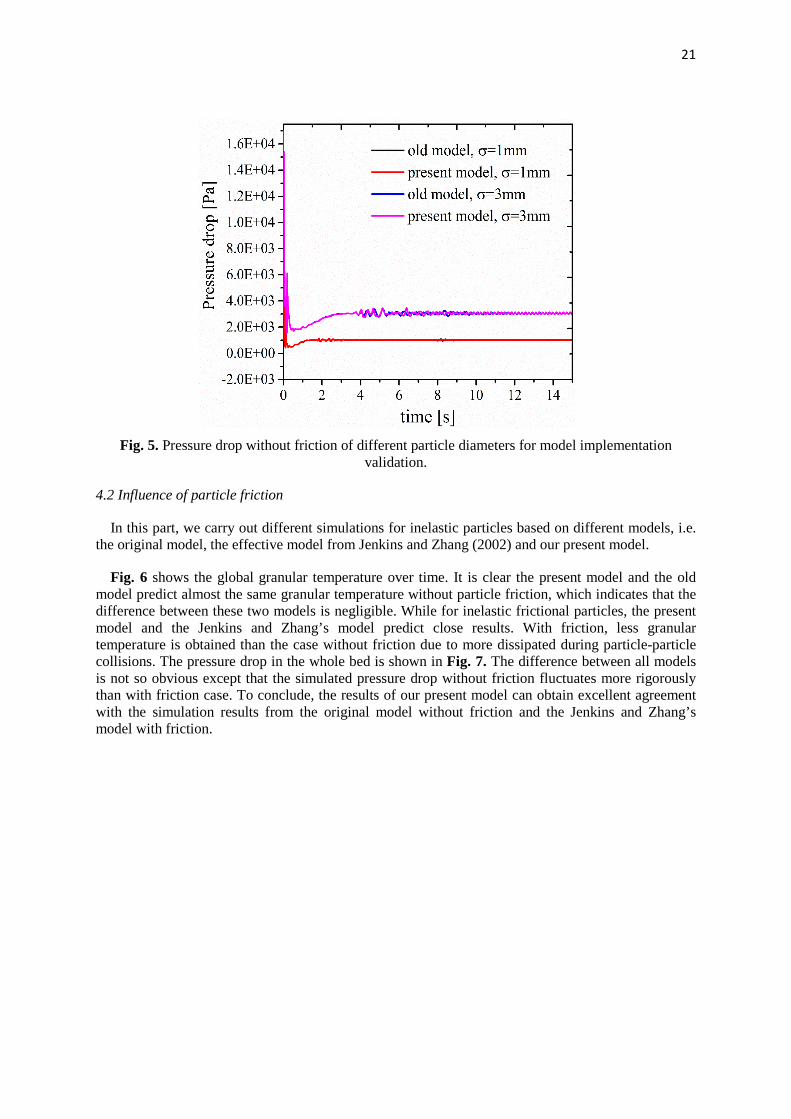
Fig. 4 shows that at the first 2 seconds, the granular temperature increases quickly and then decrease sharply because of the injection of gas. From Fig. 5, it should be noted that a significant decrease in pressure drop is observed before the full fluidization takes place, and then the pressure drop tends to be steady because ideal particles are used. The same simulation results are obtained for our new model, both for small and big particles, which validates the implementation of the new model in the code for ideal particles. In the next session, we will focus on validation of the present model by comparing with results obtained from Jenkins and Zhang’s model for simulation of non-ideal frictional particles.

Fig. 4. Granular temperatures without friction of different particle diameters for model

implementation validation.

21

Fig. 5. Pressure drop without friction of different particle diameters for model implementation

validation.

4.2 Influence of particle friction

In this part, we carry out different simulations for inelastic particles based on different models, i.e. the original model, the effective model from Jenkins and Zhang (2002) and our present model.

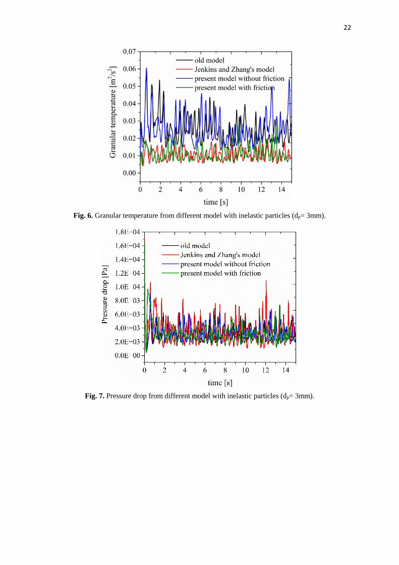
Fig. 6 shows the global granular temperature over time. It is clear the present model and the old model predict almost the same granular temperature without particle friction, which indicates that the difference between these two models is negligible. While for inelastic frictional particles, the present model and the Jenkins and Zhang’s model predict close results. With friction, less granular temperature is obtained than the case without friction due to more dissipated during particle-particle collisions. The pressure drop in the whole bed is shown in Fig. 7. The difference between all models is not so obvious except that the simulated pressure drop without friction fluctuates more rigorously than with friction case. To conclude, the results of our present model can obtain excellent agreement with the simulation results from the original model without friction and the Jenkins and Zhang’s model with friction.

22

Fig. 6. Granular temperature from different model with inelastic particles (dp= 3mm).

Fig. 7. Pressure drop from different model with inelastic particles (dp= 3mm).

23

Fig. 8. Time-averaged (1-15 s) translational granular temperature over solids concentration with

different models at Ug=2.35 m/s in the bed height from 0-0.47 m (dp= 3mm).

Fig. 8 shows the quantitatively comparison of translational granular temperature profiles from different models over solids concentration. The predicted translational granular temperatures from all models increase with the increase of solids concentration. For dilute regime, the granular temperature is proportional to the 2/3 power of the solids concentration, as is reported by Gidaspow (1994). In the transition region (solids concentration between 0.35-0.4), granular temperature reached maxium, which has been also observed by Lu et al. (2003) and Wang et al. (2012b). Without friction, the present model and the original model predicts almost similar profile which again indicates negligible difference between these two models. With friction, both our present model and Jenkins and Zhang’s model predict similar and low granular temperature. In conclusion, the present model can be employed to gas-solids bubbling fluidized beds considering particle friction.

5. Conclusions

We have extended the kinetic theory of granular flow to include angular momenta of rough spheres, using the Chapman-Enskog method for the derivation of the balance laws and Grad’s moment solution for higher order perturbation functions. In this theory, the transition between sticking and sliding collisions is distinguished. The new model accounts for the dependence on friction coefficient explicitly. The model has been incorporated into our in-house two fluid model code. Comparison between the new model and the original KTGF code was carried out using the same boundary conditions for the case of perfectly elastic particles. The simulation results show that the implementation of the presented model is right. Besides, the present model and the model from Jenkins and Zhang (2002) are applied to investigate the effect of particle friction. Results show that our present model can obtain close agreement with Jenkins and Zhang’s model.

In the next part, the developed model and its numerical implementation will be tested for a more realistic gas-solid fluidized bed containing frictional inelastic spheres. Simulation results for the granular temperature, solid velocity, particle circulation pattern and particle density function will be compared against the model from Jenkins and Zhang (2002) and Euler-Lagrange computations.

Nomenclature

c translational particle velocity, m/s v mean particle translational velocity, m/s C translational fluctuating particle velocity, m/s

24

'c translational particle velocity after collision, m/s G relative particle velocity at contact point, m/s J impulse force, kg m/s k unit normal vector at contact point j unit tangential vector at contact point F external body force (acceleration) acting on the particle, m/s2

T external torque (angular acceleration) acting on the particle, rad/s2 g gravitational acceleration, m/s2 r position of the particle, m f(0) single particle distribution function, first approximation (Maxwellian) f(1) single particle distribution function, second approximation f(2) pair particle distribution function I moment of inertia, kg m2 m mass of the particle, kg n particle number density, m-3

Umf minimum fluidization velocity, m/s e normal restitution coefficient

Greek

ρ density, kg/m3

Θ granular temperature, m2/s2

β0 tangential restitution coefficient σ particle diameter, m γ energy dissipation rate, J/(m3s) βA inter-phase momentum transfer coefficient, kg/(m3s) τ stress tensor (Pa) ε volume fraction ω rotational velocity, rad/s κ thermal conductivity, kg/(m∙s) χc collisional source of particle properties θc collisional flux of particle properties Ω rotational fluctuating particle velocity, rad/s µt translational shear viscosity, kg/(m∙s) Subscript

1 particle 1 2 particle 2 s solid phase r rotational contribution i coordinate direction i j coordinate direction j k coordinate direction k n normal direction w wall

Acknowledgment

The authors would like to thank the European Research Council for its financial support, under its Advanced Investigator Grant scheme, Contract no. 247298 (Multi-scale Flows).

References

Abu-Zaid, S., Ahmadi, G., 1990. Simple kinetic model for rapid granular flows including frictional losses. Journal of Engineering Mechanics 116, 379-389.

25

Beetstra, R., Van der Hoef, M. A., Kuipers, J. A. M., 2007. Drag force of intermediate Reynolds number flow past mono- and bidisperse arrays of spheres. AIChE Journal 53, 489-501.

Chapman, S., Cowling, T. G., 1970. The Mathematical Theory of Non-Uniform Gases, 3rd ed. Cambridge University Press, Cambridge.

Chou, C. S., Richman, M. W., 1998. Constitutive theory for homogeneous granular shear flows of highly inelastic spheres. Physica A: Statistical Mechanics and its Applications 259, 430-448.

Chen, J., Wang, S., Sun, D., Lu, H., Gidaspow, D., Yu, H., 2012) A second-order moment method applied to gas-solid risers. AIChE Journal 58, 3653-3675.

Chialvo, S., Sun, J., Sundaresan, S., 2012. Bridging the rheology of granular flows in three regimes. Physical Review E 85, 021305.

Chialvo, S., Sundaresan, S., 2013. A modified kinetic theory for frictional granular flows in dense and dilute regimes. Physics of Fluids 25, 070603.

Davidson, J. F., Cliff, R., Harrison, D. (eds), 1985. Fluidization, 2nd ed. Academic Press, London, UK.

Ding, J. M., Gidaspow, D., 1990. A bubbling fluidization model using kinetic theory of granular flow. AIChE Journal 36, 523-538.

Enwald, H., Peirano, E., Almstedt, A. E., 1996. Eulerian two-phase flow theory applied to fluidization. International Journal of Multiphase Flow 22 (Sup.), 21-66.

Foerster, S. F., Louge, M. Y., Chang, H., Allia, K., 1994. Measurements of the collision properties of small spheres. Physics of Fluids 6, 1108-1115.

Grad, H., 1949. On the kinetic theory of rarefied gases. Communications on Pure and Applied Mathematics 2, 331-407.

Gidaspow, D., 1994. Multiphase Flow and Fluidization: Continuum and Kinetic Theory Descriptions. Academic Press Inc., Boston.

Goldshtein, A., Shapiro, M., 1995. Mechanics of collisional motion of granular materials. Part 1. General hydrodynamic equations. Journal of Fluid Mechanics 282, 75-114.

Garzó, V., Dufty, J. W., 1999. Dense fluid transport for inelastic hard spheres. Physical Review E 59, 5895-5911.

Goldschmidt, M. J. V., Kuipers, J. A. M., van Swaaij, W. P. M., 2001. Hydrodynamic modeling of dense gas-fluidised beds using the kinetic theory of granular flow: effect of coefficient of restitution on bed dynamics. Chemical Engineering Science 56, 571-78.

Harlow, F. H., Amsden, A. A., 1974. Kachina: an Eulerian Computer Program for Multifield Fluid Flows. Los Alamos, Report.

Davidson, J. F., Clift, R., Harrison, D., 1985. Fluidization, Academic press, London. Jenkins, J. T., Savage, S. B., 1983. A theory for the rapid flow of identical, smooth, nearly elastic,

spherical particles. Journal of Fluid Mechanics 30, 187-202. Jenkins, J. T., Richman, M. W., 1985. Grad's 13-moment system for a dense gas of inelastic spheres.

Archive for Rotational Mechanics and Analysis 87, 355-377. Jenkins, J. T., Zhang, C., 2002. Kinetic theory for identical, frictional, nearly elastic spheres. Physics

of Fluids 14, 1228-1235. Kunii, D., Levenspiel, O., 1991. Fluidization Engineering, 2nd edition, Butterworth-Heinemann,

Boston. Kumaran, V., 2004. Constitutive relations and linear stability of a sheared granular flow. Journal of

Fluid Mechanics 506, 1-43. Kumaran, V., 2006. The constitutive relation for the granular flow of rough particles, and its

application to the flow down an inclined plane. Journal of Fluid Mechanics 561, 1-42. Kuipers, J. A. M., van Duin, K. J., van Beckum, F. P. H., and van Swaaij, W. P. M., 1992. A

numerical model of gas-fluidized beds. Chemical Engineering Science 47, 1913-1924. Lun, C. K. K., Savage, S. B., Jeffrey D. J., Chepurniy N., 1984. Kinetic theories for granular flow:

inelastic particles in Couette flow and slightly inelastic particles in a general flow field. Journal of Fluid Mechanics 140, 223-256.

Lun, C. K. K., Savage, S. B., 1987. A simple kinetic theory for granular flow of rough, inelastic, spherical particles. Journal of Application Mechanics 54, 47-53.

Lun, C. K. K., 1991. Kinetic theory for granular flow of dense, slightly inelastic, slightly rough spheres. Journal of Application Mechanics 233, 539-559.

26

Lu, H. L., Gidaspow, D., 2003. Hydrodynamics of binary fluidization in a riser: CFD simulation using two granular temperatures. Chemical Engineering Science 58, 3777-3792.

Lu, H. L., Gidaspow, D., Bouillard, J., Wentie, L., 2003. Hydrodynamic simulation of gas–solid flow in a riser using kinetic theory of granular flow. Chemical Engineering Journal 95, 1-13.

Ma, D., Ahmadi, G., 1986. An equation of state for dense rigid sphere gases. The Journal of Chemical Physics 84, 3449-3450.

Nieuwland, J. J., 1995. Hydrodynamic Modelling of Gas-Solid Two-Phase Flows (Ph.D. thesis). Twente University, Enschede, the Netherlands.

Patankar, S. V., Spalding, D. B., 1972. A calculation procedure for heat, mass and momentum transfer in three-dimensional parabolic flows. International Journal of Heat and Mass Transfer 15, 1787-1806.

Rao, K. K., Nott, P. R., 2008. An introduction to granular flow. New York: Cambridge University Press. Chapter 9.

Sun, D., Wang, S. Y., W., Lu, H. L., Shen, Z. H., Li, X., Wang, S., Zhao, Y. H., Wei, L. X., 2009. A second-order moment method of dense gas–solid flow for bubbling fluidization. Chemical Engineering Science 64, 5013-5027.

Sun, J., Sundaresan, S., 2011. A constitutive model with microstructure evolution for flow of rate-independent granular materials. Journal of Fluid Mechanics 682, 590-616.

Verma, V., Deen, N. G., Padding, J. T., Kuipers, J. A. M., 2013. Two-fluid modeling of three-dimensional cylindrical gas-solid fluidized beds using the kinetic theory of granular flow. Chemical Engineering Science 102, 227-245.

Walton, O. R., 1992. Numerical simulation of inelastic, frictional particle-particle interactions, in Particulate Two-Phase Flow, Part I, edited by M.C. Roco, Butterworth-Heinemann, Boston, 884.

Wang, S., Hao, Z. H., Lu, H. L., Liu, G. D., Wang, J. X., Xu, P. F., 2012a. A bubbling fluidization model using kinetic theory of rough spheres. AIChE Journal 58, 440-455.

Wang, S., Liu, G., Lu, H. L., Sun, L., Xu, P., 2012b. CFD simulation of bubbling fluidized beds using kinetic theory of rough sphere. Chemical Engineering Science 71, 185-201.

Zhao, Y., Lu, B., Zhong, Y., 2013. Euler-Euler modeling of a gas-solid bubbling fluidized bed with kinetic theory of rough particles. Chemical Engineering Science 104, 767-779.

Appendix A

All the basic integrals which be solved using Mathematica, is listed as follows,

( )( )*

2 2 2

1 32

sin cos11 cos

u uu

u

a dπ

θ

θ θλ θλ θ

= ++

∫ (A1)

( )( )

* 3

2 320

sin cos11 cos

u uu

u

a dθ θ θλ θ

λ θ= +

+∫ (A2)

( )( )*

2 3

3 32

sin cos11 cos

u u

u

a dπ

θ

θ θλ θλ θ

= ++

∫ (A3)

( )( )*

2 2 3

4 7 22

sin cos11 cos

u uu

u

a dπ

θ

θ θλ θλ θ

= ++

∫ (A4)

( )( )

* 3 23 2

5 320

sin cos11 cos

u uu

u

a dθ θ θλ θ

λ θ= +

+∫ (A5)

( )( )*

2 43 2

6 7 22

cos sin11 cos

u uu

u

a dπ

θ

θ θλ θλ θ

= ++

∫ (A6)

27

( )( )*

2 3

7 32

cos sin11 cos

u uu

u

a dπ

θ

θ θλ θλ θ

= ++

∫ (A7)

( )( )*

2 3 23 2

8 7 22

sin cos11 cos

uu u

u

daπ

θ

θθ θλ

λ θ= +

+∫ (A8)

( )( )

* 3 3

9 420

sin cos11 cos

u uu

u

a dθ θ θλ θ

λ θ= +

+∫ (A9)

( )( )*

/2 3 3

10 42

sin cos11 cos

u uu

u

a dπ

θ

θ θλ θλ θ

= ++

∫ (A10)

( )( )*

/2 2 4

11 42

sin cos11 cos

u uu

u

a dπ

θ

θ θλ θλ θ

= ++

∫ (A11)

( )( )*

/2 4 2

12 42

sin cos11 cos

u uu

u

a dπ

θ

θ θλ θλ θ

= ++

∫ (A12)

( )( )*

/2 5

13 42

sin cos11 cos

u uu

u

a dπ

θ

θ θλ θλ θ

= ++

∫ (A13)

( )( )

* 5

14 420

sin cos11 cos

u uu

u

a dθ θ θλ θ

λ θ= +

+∫ (A14)

( )*

/2 3

15 42

sin cos

1 cosu u

u

u

a dπ

θ

θ θ θλ θ

=+

∫ (A15)

( )

* 3

16 420

sin cos

1 cosu u

u

u

a dθ θ θ θ

λ θ=

+∫ (A16)

( )*

/2 2 2

17 42

sin cos

1 cosu u

u

u

a dπ

θ

θ θ θλ θ

=+

∫ (A17)

Integrals appear in the closure equations,

( )1 1 1 2 2A a aµη η= − + (A18)

( ) ( ) ( )2 22 1 3 2 2A 1 a aλ µη η = + + (A19)

( )3 1 4 2 5A a aµη η= − + (A20)

( ) ( ) ( )2 24 1 6 2 5A 1 a aλ µη η = + + (A21)

( ) ( ) ( )2 25 1 1 2 2A 1 a aλ µη η = + + (A22)

( )6 1 11 2 9A a aµη η= − + (A23)

28

( )7 1 12 2 14A a aµη η= − + (A24)

( ) ( )2 28 1 12 2 14A a aµη η= + (A25)

( )9 1 17 2 16A a aµη η= − + (A26)

( ) ( )2 210 1 17 2 16A a aµη η= + (A27)

( ) ( )2 211 1 10 2 14A a aµη η= + (A28)

( ) ( )2 212 1 15 2 16A a aµη η= + (A29)

( ) ( )2 213 1 13 2 9A a aµη η= + (A30)

Appendix B

The solutions of the related integrals in equations (2.23-25) are given as follows. For the flux term:

( ) ( )

( ) ( )

1 1 1 220

1 1 4 3

192

12

(1 ) 2 1 A 1 A1( )2

(1 ) +5 1 A 2 1 A

t

c i i s t s

s

mc c gη η λ λ

χ ρ ε σ πη η λ λ

−

+

Θ+ − + + + = Θ

∇ ⋅ + + − + v

(B1)

( ) ( )20 2 1 4 3120

1 96( ) 2.5A A 2.5A A2

tc i i s t s sI gχ ω ω ρ ε λ λ

σ π− +

Θ = Θ − ∇ ⋅ −

v (B2)

( ) ( ) ( ),2 1

0 11

( )2

16 1 2 1 A4 1c j

t ti i s s

j

mC C gr

ηθ λ σρ ε λλ π

Θ ∂Θ= + + + + ∂

(B3)

( ) 2, 0 1

1( ) 16 1 A2

t t rc j i i s s

r j

I gr

θ λ λ σ ρ επ

Θ Θ ∂ΘΩΩ = − +

Θ ∂ (B4)

( )

( )

,2 2

0 0

1

1

( ) 2(1 ) 48 1

( )

2 1 5 3[ ( ) ( ) ]A15 2

30(1

2

)

c jt

i ij t s s s s

ji kij

j i k

j ji i kij

j i j i k

mC e g g

vv vx x x

v vv v vx x x x x

θ δ ρ ε λ σρ επ

η δλ

λδ

Θ= + Θ − +

∂ ∂ ∂−+ + ∂ ∂ ∂

∂ ∂+ ∂ ∂ ∂ + − + + − ∂ ∂ ∂ ∂ ∂

+ (B5)

( )( )( )

( ) ( ), 0

21 1

12

1 4 3

30 3 2 2 380 140 701 6 15 1 15( )2 10

20 1 2 A 2 1 2 Ac l i j j li s s tmC C C g

η ηλ ληλθ δ ρ ε

η λ

=

+ ++ ++ +− Θ

+ + − +

(B6)

( ) ( ),2 2 1

0 1 3 42 (6 13)( ) 6 10(1 2 ) 2 A 5A

15 1c l j j i li s s tI C g λη λθ δ ρ ε η λλ

+Ω Ω = − Θ + − − +

(B7)

29

( ) ( )( )

( )( ) ( )

( ) ( )( ) ( ) ( ) ( )( )

20

3 22

1 1 1 1 62

229 7 13 12

192( )15

16 18 32 1 1 0.5 9 1 4 1 2 A 0.5 11 12 33 1

3 1 (4 3) 1 A 6 1 2 A 3 1 A 0.5 1 2 A

mnt

mn j i s s ijFa mC C g aρ εσ π

λ λ λη η η η λ λ λλ

λ λ λ λ λ λ λ λ λ λ

Θ=

+ + + + + − + + + − + + +

− + + + + + + + + − + +

(B8)

( )( ) ( )( )

0

212 1

1 1 1 3 4

( ) 12

4 8 10 2.543 3 10 1 1 2 A 5A3 15 1

tc i j j s s s t

i

mC C C gx

χ ε ε ρ

η λ λληη η η λλ

∂Θ= − Θ

∂

+ + + + + − + + + +

(B9)

0

2

1 2

1 2

2

22 1 57 8

320( )

10.5(11 12 3) 10.5 ( 2)( 3) 61(1 )450( 1) 450

(11 12 3) ( 2)( 3)75( 1)

140A 116(2 1)A 24A 0.04(102 272 6)(A A )315

0

kmn kmns s s ipp t

i j ja Fg a

C C Cε ε ρ

σ π

λ λ λ λ ληλ

ηλ λ λ λ λ

λλ λ λ

− Θ=

+ + + + ++ + + − + + + + + +

+ + + −

+ − + + +

− ( )( )

2 210 9

1 6

.04[ 1 (96 99 21) 9 ](A A )

0.48(1 )(2 1) 1 A

λ λ λ λ

η λ λ

+ + + + + − − + +

( B10)

( )

21 11

0

12 9

50A 10010A A32 3( )50 2025 ( 1)( 2) A 3 4 A3 3

kmn kmn ipps s s t

j j iDgb I C bσε ε ρ λ

π λ λ λλ

− − − ΘΩ Ω =

− + + + +

(B11)

( ) ( )0

21 1

2 1 1 4 1 330(4 3)24 20 505 6 (40 10)A 20 2 1 A

15 1 1550

sN g η ηλ λε η η η λλ

+ −− + + = − + + − + + +

(B12)

2 ( )mnt j i ijFM mC C aΘ = (B13)

1 ( )kmn ipps s i j jF aN C C Cε ρ = (B14)

1 ( )kmn ipps s j j iDL I C bε ρ = Ω Ω (B15)

( ) ( )12 0 1 3 4

56 ( 2) 60(1 4 ) 2A 5A5 1s tL g η λ λε η λ

λ +

= Θ − + − + (B16)

13 0 1 3

8 )12(1 ) 50(1(2 )A5 3(1 )s tL g η λε λ η

λ

= + Θ − + ++

+ (B17)