Modern Thermodynamics - Av8n. · PDF fileModern Thermodynamics John Denker. ii Modern...

Modern Thermodynamics

John Denker

ii Modern Thermodynamics

Contents

0 Introduction 01

0.1 Overview . . . . . . . . . . . . . . . . . . . . . . . . . . . . . . . . . . . . . 01

0.2 Availability . . . . . . . . . . . . . . . . . . . . . . . . . . . . . . . . . . . . 03

0.3 Prerequisites, Goals, and Non-Goals . . . . . . . . . . . . . . . . . . . . . . 03

1 Energy 11

1.1 Preliminary Remarks . . . . . . . . . . . . . . . . . . . . . . . . . . . . . . 11

1.2 Conservation of Energy . . . . . . . . . . . . . . . . . . . . . . . . . . . . . 12

1.3 Examples of Energy . . . . . . . . . . . . . . . . . . . . . . . . . . . . . . . 13

1.4 Remark: Recursion . . . . . . . . . . . . . . . . . . . . . . . . . . . . . . . 15

1.5 Energy is Completely Abstract . . . . . . . . . . . . . . . . . . . . . . . . . 15

1.6 Additional Remarks . . . . . . . . . . . . . . . . . . . . . . . . . . . . . . . 16

1.7 Energy versus Capacity to do Work or Available Energy . . . . . . . . . 18

1.7.1 Best Case : Non-Thermal Situation . . . . . . . . . . . . . . . . . . 18

1.7.2 Equation versus Denition . . . . . . . . . . . . . . . . . . . . . . . 18

1.7.3 General Case : Some Energy Not Available . . . . . . . . . . . . . . 19

1.8 Mutations . . . . . . . . . . . . . . . . . . . . . . . . . . . . . . . . . . . . 114

1.8.1 Energy . . . . . . . . . . . . . . . . . . . . . . . . . . . . . . . . . . 114

1.8.2 Conservation . . . . . . . . . . . . . . . . . . . . . . . . . . . . . . 114

1.8.3 Energy Conservation . . . . . . . . . . . . . . . . . . . . . . . . . . 115

1.8.4 Internal Energy . . . . . . . . . . . . . . . . . . . . . . . . . . . . . 115

1.9 Range of Validity . . . . . . . . . . . . . . . . . . . . . . . . . . . . . . . . 115

iv CONTENTS

2 Entropy 21

2.1 Paraconservation . . . . . . . . . . . . . . . . . . . . . . . . . . . . . . . . 21

2.2 Scenario: Cup Game . . . . . . . . . . . . . . . . . . . . . . . . . . . . . . 22

2.3 Scenario: Card Game . . . . . . . . . . . . . . . . . . . . . . . . . . . . . . 23

2.4 Peeking . . . . . . . . . . . . . . . . . . . . . . . . . . . . . . . . . . . . . . 25

2.5 Discussion . . . . . . . . . . . . . . . . . . . . . . . . . . . . . . . . . . . . 26

2.5.1 Connecting Models to Reality . . . . . . . . . . . . . . . . . . . . . 26

2.5.2 States and Probabilities . . . . . . . . . . . . . . . . . . . . . . . . 28

2.5.3 Entropy is Not Knowing . . . . . . . . . . . . . . . . . . . . . . . . 29

2.5.4 Entropy versus Energy . . . . . . . . . . . . . . . . . . . . . . . . . 29

2.5.5 Entropy versus Disorder . . . . . . . . . . . . . . . . . . . . . . . . 210

2.5.6 False Dichotomy, or Not . . . . . . . . . . . . . . . . . . . . . . . . 212

2.5.7 dQ, or Not . . . . . . . . . . . . . . . . . . . . . . . . . . . . . . . 213

2.6 Quantifying Entropy . . . . . . . . . . . . . . . . . . . . . . . . . . . . . . 213

2.7 Microstate versus Macrostate . . . . . . . . . . . . . . . . . . . . . . . . . . 216

2.7.1 Surprisal . . . . . . . . . . . . . . . . . . . . . . . . . . . . . . . . . 216

2.7.2 Contrasts and Consequences . . . . . . . . . . . . . . . . . . . . . . 217

2.8 Entropy of Independent Subsystems . . . . . . . . . . . . . . . . . . . . . . 218

3 Basic Concepts (Zeroth Law) 31

4 Low-Temperature Entropy (Alleged Third Law) 41

5 The Rest of Physics, Chemistry, etc. 51

6 Classical Thermodynamics 61

6.1 Overview . . . . . . . . . . . . . . . . . . . . . . . . . . . . . . . . . . . . . 61

6.2 Stirling Engine . . . . . . . . . . . . . . . . . . . . . . . . . . . . . . . . . . 61

6.2.1 Basic Structure and Operations . . . . . . . . . . . . . . . . . . . . 61

6.2.2 Energy, Entropy, and Eciency . . . . . . . . . . . . . . . . . . . . 66

CONTENTS v

6.2.3 Practical Considerations; Temperature Match or Mismatch . . . . . 69

6.2.4 Discussion: Reversibility . . . . . . . . . . . . . . . . . . . . . . . . 610

6.3 All Reversible Heat Engines are Equally Ecient . . . . . . . . . . . . . . . 611

6.4 Not Everything is a Heat Engine . . . . . . . . . . . . . . . . . . . . . . . . 611

6.5 Carnot Eciency Formula . . . . . . . . . . . . . . . . . . . . . . . . . . . 612

6.5.1 Denition of Heat Engine . . . . . . . . . . . . . . . . . . . . . . . 612

6.5.2 Analysis . . . . . . . . . . . . . . . . . . . . . . . . . . . . . . . . . 614

6.5.3 Discussion . . . . . . . . . . . . . . . . . . . . . . . . . . . . . . . . 615

7 Functions of State 71

7.1 Functions of State : Basic Notions . . . . . . . . . . . . . . . . . . . . . . . 71

7.2 Path Independence . . . . . . . . . . . . . . . . . . . . . . . . . . . . . . . 72

7.3 Hess's Law, Or Not . . . . . . . . . . . . . . . . . . . . . . . . . . . . . . . 74

7.4 Partial Derivatives . . . . . . . . . . . . . . . . . . . . . . . . . . . . . . . . 75

7.5 Heat Capacities, Energy Capacity, and Enthalpy Capacity . . . . . . . . . . 79

7.6 E as a Function of Other Variables . . . . . . . . . . . . . . . . . . . . . . 714

7.6.1 V , S, and h . . . . . . . . . . . . . . . . . . . . . . . . . . . . . . . 714

7.6.2 X, Y , Z, and S . . . . . . . . . . . . . . . . . . . . . . . . . . . . . 717

7.6.3 V , S, and N . . . . . . . . . . . . . . . . . . . . . . . . . . . . . . 718

7.6.4 Yet More Variables . . . . . . . . . . . . . . . . . . . . . . . . . . . 719

7.7 Internal Energy . . . . . . . . . . . . . . . . . . . . . . . . . . . . . . . . . 720

7.8 Integration . . . . . . . . . . . . . . . . . . . . . . . . . . . . . . . . . . . . 723

7.9 Advection . . . . . . . . . . . . . . . . . . . . . . . . . . . . . . . . . . . . 724

7.10 Deciding What's True . . . . . . . . . . . . . . . . . . . . . . . . . . . . . . 724

7.11 Deciding What's Fundamental . . . . . . . . . . . . . . . . . . . . . . . . . 726

vi CONTENTS

8 Thermodynamic Paths and Cycles 81

8.1 A Path Projected Onto State Space . . . . . . . . . . . . . . . . . . . . . . 81

8.1.1 State Functions . . . . . . . . . . . . . . . . . . . . . . . . . . . . . 81

8.1.2 Out-of-State Functions . . . . . . . . . . . . . . . . . . . . . . . . . 84

8.1.3 Converting Out-of-State Functions to State Functions . . . . . . . . 85

8.1.4 Reversibility and/or Uniqueness . . . . . . . . . . . . . . . . . . . . 86

8.1.5 The Importance of Out-of-State Functions . . . . . . . . . . . . . . 87

8.1.6 Heat Content, or Not . . . . . . . . . . . . . . . . . . . . . . . . . . 87

8.1.7 Some Mathematical Remarks . . . . . . . . . . . . . . . . . . . . . 88

8.2 Grady and Ungrady One-Forms . . . . . . . . . . . . . . . . . . . . . . . . 88

8.3 Abuse of the Notation . . . . . . . . . . . . . . . . . . . . . . . . . . . . . . 811

8.4 Procedure for Extirpating dW and dQ . . . . . . . . . . . . . . . . . . . . . 811

8.5 Some Reasons Why dW and dQ Might Be Tempting . . . . . . . . . . . . . 812

8.6 Boundary versus Interior . . . . . . . . . . . . . . . . . . . . . . . . . . . . 815

8.7 The Carnot Cycle . . . . . . . . . . . . . . . . . . . . . . . . . . . . . . . . 816

9 Connecting Entropy with Energy 91

9.1 The Boltzmann Distribution . . . . . . . . . . . . . . . . . . . . . . . . . . 91

9.2 Systems with Subsystems . . . . . . . . . . . . . . . . . . . . . . . . . . . . 91

9.3 Remarks . . . . . . . . . . . . . . . . . . . . . . . . . . . . . . . . . . . . . 94

9.3.1 Predictable Energy is Freely Convertible . . . . . . . . . . . . . . . 94

9.3.2 Thermodynamic Laws without Temperature . . . . . . . . . . . . . 94

9.3.3 Kinetic and Potential Microscopic Energy . . . . . . . . . . . . . . 94

9.3.4 Ideal Gas : Potential Energy as well as Kinetic Energy . . . . . . . 96

9.3.5 Relative Motion versus Thermal Energy . . . . . . . . . . . . . . 97

9.4 Entropy Without Constant Re-Shuing . . . . . . . . . . . . . . . . . . . . 98

9.5 Units of Entropy . . . . . . . . . . . . . . . . . . . . . . . . . . . . . . . . . 910

9.6 Probability versus Multiplicity . . . . . . . . . . . . . . . . . . . . . . . . . 911

9.6.1 Exactly Equiprobable . . . . . . . . . . . . . . . . . . . . . . . . . 911

CONTENTS vii

9.6.2 Approximately Equiprobable . . . . . . . . . . . . . . . . . . . . . 913

9.6.3 Not At All Equiprobable . . . . . . . . . . . . . . . . . . . . . . . . 915

9.7 Discussion . . . . . . . . . . . . . . . . . . . . . . . . . . . . . . . . . . . . 916

9.8 Misconceptions about Spreading . . . . . . . . . . . . . . . . . . . . . . . . 917

9.9 Spreading in Probability Space . . . . . . . . . . . . . . . . . . . . . . . . . 921

10 Additional Fundamental Notions 101

10.1 Equilibrium . . . . . . . . . . . . . . . . . . . . . . . . . . . . . . . . . . . 101

10.2 Non-Equilibrium; Timescales . . . . . . . . . . . . . . . . . . . . . . . . . . 102

10.3 Eciency; Timescales . . . . . . . . . . . . . . . . . . . . . . . . . . . . . . 103

10.4 Spontaneity and Irreversibility . . . . . . . . . . . . . . . . . . . . . . . . . 104

10.5 Stability . . . . . . . . . . . . . . . . . . . . . . . . . . . . . . . . . . . . . 105

10.6 Relationship between Static Stability and Damping . . . . . . . . . . . . . 107

10.7 Finite Size Eects . . . . . . . . . . . . . . . . . . . . . . . . . . . . . . . . 107

10.8 Words to Live By . . . . . . . . . . . . . . . . . . . . . . . . . . . . . . . . 1010

11 Experimental Basis 111

11.1 Basic Notions of Temperature and Equilibrium . . . . . . . . . . . . . . . . 111

11.2 Exponential Dependence on Energy . . . . . . . . . . . . . . . . . . . . . . 112

11.3 Metastable Systems with a Temperature . . . . . . . . . . . . . . . . . . . 113

11.4 Metastable Systems without a Temperature . . . . . . . . . . . . . . . . . . 116

11.5 Dissipative Systems . . . . . . . . . . . . . . . . . . . . . . . . . . . . . . . 117

11.5.1 Sudden Piston : Sound . . . . . . . . . . . . . . . . . . . . . . . . . 117

11.5.2 Sudden Piston : State Transitions . . . . . . . . . . . . . . . . . . . 1110

11.5.3 Rumford's Experiment . . . . . . . . . . . . . . . . . . . . . . . . . 1113

11.5.4 Simple Example: Decaying Current . . . . . . . . . . . . . . . . . . 1115

11.5.5 Simple Example: Oil Bearing . . . . . . . . . . . . . . . . . . . . . 1115

11.5.6 Misconceptions : Heat . . . . . . . . . . . . . . . . . . . . . . . . . 1118

11.5.7 Misconceptions : Work . . . . . . . . . . . . . . . . . . . . . . . . . 1119

viii CONTENTS

11.5.8 Remarks . . . . . . . . . . . . . . . . . . . . . . . . . . . . . . . . . 1119

11.6 The Gibbs Gedankenexperiment . . . . . . . . . . . . . . . . . . . . . . . . 1119

11.7 Spin Echo Experiment . . . . . . . . . . . . . . . . . . . . . . . . . . . . . 1121

11.8 Melting . . . . . . . . . . . . . . . . . . . . . . . . . . . . . . . . . . . . . . 1121

11.9 Isentropic Expansion and Compression . . . . . . . . . . . . . . . . . . . . 1121

11.10 Demagnetization Refrigerator . . . . . . . . . . . . . . . . . . . . . . . . . 1122

11.11 Thermal Insulation . . . . . . . . . . . . . . . . . . . . . . . . . . . . . . . 1123

12 More About Entropy 121

12.1 Terminology: Microstate versus Macrostate . . . . . . . . . . . . . . . . . . 121

12.2 What the Second Law Doesn't Tell You . . . . . . . . . . . . . . . . . . . . 122

12.3 Phase Space . . . . . . . . . . . . . . . . . . . . . . . . . . . . . . . . . . . 124

12.4 Entropy in a Crystal; Phonons, Electrons, and Spins . . . . . . . . . . . . . 126

12.5 Entropy is Entropy . . . . . . . . . . . . . . . . . . . . . . . . . . . . . . . 127

12.6 Spectator Entropy . . . . . . . . . . . . . . . . . . . . . . . . . . . . . . . . 128

12.7 No Secret Entropy, No Hidden Variables . . . . . . . . . . . . . . . . . . . 128

12.8 Entropy is Context Dependent . . . . . . . . . . . . . . . . . . . . . . . . . 1210

12.9 Slice Entropy and Conditional Entropy . . . . . . . . . . . . . . . . . . . . 1212

12.10 Extreme Mixtures . . . . . . . . . . . . . . . . . . . . . . . . . . . . . . . . 1213

12.10.1 Simple Model System . . . . . . . . . . . . . . . . . . . . . . . . . 1213

12.10.2 Two-Sample Model System . . . . . . . . . . . . . . . . . . . . . . 1214

12.10.3 Helium versus Snow . . . . . . . . . . . . . . . . . . . . . . . . . . 1216

12.10.4 Partial Information aka Weak Peek . . . . . . . . . . . . . . . . . . 1216

12.11 Entropy is Not Necessarily Extensive . . . . . . . . . . . . . . . . . . . . . 1217

12.12 Mathematical Properties of the Entropy . . . . . . . . . . . . . . . . . . . . 1218

12.12.1 Entropy Can Be Innite . . . . . . . . . . . . . . . . . . . . . . . . 1218

CONTENTS ix

13 Temperature : Denition and Fundamental Properties 131

13.1 Example Scenario: Two Subsystems, Same Stu . . . . . . . . . . . . . . . 131

13.1.1 Equilbrium is Isothermal . . . . . . . . . . . . . . . . . . . . . . . . 137

13.2 Remarks about the Simple Special Case . . . . . . . . . . . . . . . . . . . . 138

13.3 Two Subsystems, Dierent Stu . . . . . . . . . . . . . . . . . . . . . . . . 138

13.4 Discussion: Constants Drop Out . . . . . . . . . . . . . . . . . . . . . . . . 139

13.5 Calculations . . . . . . . . . . . . . . . . . . . . . . . . . . . . . . . . . . . 1313

13.6 Chemical Potential . . . . . . . . . . . . . . . . . . . . . . . . . . . . . . . 1313

14 Spontaneity, Reversibility, Equilibrium, Stability, Solubility, etc. 141

14.1 Fundamental Notions . . . . . . . . . . . . . . . . . . . . . . . . . . . . . . 141

14.1.1 Equilibrium . . . . . . . . . . . . . . . . . . . . . . . . . . . . . . . 141

14.1.2 Stability . . . . . . . . . . . . . . . . . . . . . . . . . . . . . . . . . 141

14.1.3 A First Example: Heat Transfer . . . . . . . . . . . . . . . . . . . . 141

14.1.4 Graphical Analysis One Dimension . . . . . . . . . . . . . . . . . 143

14.1.5 Graphical Analysis Multiple Dimensions . . . . . . . . . . . . . . 145

14.1.6 Reduced Dimensionality . . . . . . . . . . . . . . . . . . . . . . . . 146

14.1.7 General Analysis . . . . . . . . . . . . . . . . . . . . . . . . . . . . 147

14.1.8 What's Fundamental and What's Not . . . . . . . . . . . . . . . . 148

14.2 Proxies for Predicting Spontaneity, Reversibility, Equilibrium, etc. . . . . . 149

14.2.1 Isolated System; Proxy = Entropy . . . . . . . . . . . . . . . . . . 149

14.2.2 External Damping; Proxy = Energy . . . . . . . . . . . . . . . . . 1410

14.2.3 Constant V and T ; Proxy = Helmholtz Free Energy . . . . . . . . 1413

14.2.4 Constant P and T ; Proxy = Gibbs Free Enthalpy . . . . . . . . . . 1415

14.3 Discussion: Some Fine Points . . . . . . . . . . . . . . . . . . . . . . . . . 1418

14.3.1 Local Conservation . . . . . . . . . . . . . . . . . . . . . . . . . . . 1419

14.3.2 Lemma: Conservation of Enthalpy, Maybe . . . . . . . . . . . . . . 1419

14.3.3 Energy and Entropy (as opposed to Heat . . . . . . . . . . . . . 1420

14.3.4 Spontaneity . . . . . . . . . . . . . . . . . . . . . . . . . . . . . . . 1420

x CONTENTS

14.3.5 Conditionally Allowed and Unconditionally Disallowed . . . . . . . 1421

14.3.6 Irreversible by State or by Rate . . . . . . . . . . . . . . . . . . . . 1421

14.4 Temperature and Chemical Potential in the Equilibrium State . . . . . . . 1423

14.5 The Approach to Equilibrium . . . . . . . . . . . . . . . . . . . . . . . . . 1425

14.5.1 Non-Monotonic Case . . . . . . . . . . . . . . . . . . . . . . . . . . 1425

14.5.2 Monotonic Case . . . . . . . . . . . . . . . . . . . . . . . . . . . . . 1426

14.5.3 Approximations and Misconceptions . . . . . . . . . . . . . . . . . 1427

14.6 Natural Variables, or Not . . . . . . . . . . . . . . . . . . . . . . . . . . . . 1428

14.6.1 The Big Four Thermodynamic Potentials . . . . . . . . . . . . . . 1428

14.6.2 A Counterexample: Heat Capacity . . . . . . . . . . . . . . . . . . 1429

14.7 Going to Completion . . . . . . . . . . . . . . . . . . . . . . . . . . . . . . 1429

14.8 Example: Shift of Equilibrium . . . . . . . . . . . . . . . . . . . . . . . . . 1431

14.9 Le Châtelier's Principle, Or Not . . . . . . . . . . . . . . . . . . . . . . . 1434

14.10 Appendix: The Cyclic Triple Derivative Rule . . . . . . . . . . . . . . . . . 1436

14.10.1 Graphical Derivation . . . . . . . . . . . . . . . . . . . . . . . . . . 1436

14.10.2 Validity is Based on Topology . . . . . . . . . . . . . . . . . . . . . 1436

14.10.3 Analytic Derivation . . . . . . . . . . . . . . . . . . . . . . . . . . . 1439

14.10.4 Independent and Dependent Variables, or Not . . . . . . . . . . . . 1439

14.10.5 Axes, or Not . . . . . . . . . . . . . . . . . . . . . . . . . . . . . . 1440

14.11 Entropy versus Irreversibility in Chemistry . . . . . . . . . . . . . . . . . 1440

15 The Big Four Energy-Like State Functions 151

15.1 Energy . . . . . . . . . . . . . . . . . . . . . . . . . . . . . . . . . . . . . . 151

15.2 Enthalpy . . . . . . . . . . . . . . . . . . . . . . . . . . . . . . . . . . . . . 151

15.2.1 Integration by Parts; PV and its Derivatives . . . . . . . . . . . . . 151

15.2.2 More About PdV versus V dP . . . . . . . . . . . . . . . . . . . . . 153

15.2.3 Denition of Enthalpy . . . . . . . . . . . . . . . . . . . . . . . . . 156

15.2.4 Enthalpy is a Function of State . . . . . . . . . . . . . . . . . . . . 157

15.2.5 Derivatives of the Enthalpy . . . . . . . . . . . . . . . . . . . . . . 158

CONTENTS xi

15.3 Free Energy . . . . . . . . . . . . . . . . . . . . . . . . . . . . . . . . . . . 159

15.4 Free Enthalpy . . . . . . . . . . . . . . . . . . . . . . . . . . . . . . . . . . 159

15.5 Thermodynamically Available Energy Or Not . . . . . . . . . . . . . . . . 159

15.5.1 Overview . . . . . . . . . . . . . . . . . . . . . . . . . . . . . . . . 1510

15.5.2 A Calculation of Available Energy . . . . . . . . . . . . . . . . . . 1513

15.6 Relationships among E, F , G, and H . . . . . . . . . . . . . . . . . . . . . 1515

15.7 Yet More Transformations . . . . . . . . . . . . . . . . . . . . . . . . . . . 1517

15.8 Example: Hydrogen/Oxygen Fuel Cell . . . . . . . . . . . . . . . . . . . . . 1517

15.8.1 Basic Scenario . . . . . . . . . . . . . . . . . . . . . . . . . . . . . 1517

15.8.2 Enthalpy . . . . . . . . . . . . . . . . . . . . . . . . . . . . . . . . 1519

15.8.3 Gibbs Free Enthalpy . . . . . . . . . . . . . . . . . . . . . . . . . . 1521

15.8.4 Discussion: Assumptions . . . . . . . . . . . . . . . . . . . . . . . . 1521

15.8.5 Plain Combustion ⇒ Dissipation . . . . . . . . . . . . . . . . . . . 1522

15.8.6 Underdetermined . . . . . . . . . . . . . . . . . . . . . . . . . . . . 1528

15.8.7 H Stands For Enthalpy Not Heat . . . . . . . . . . . . . . . . 1528

16 Adiabatic Processes 161

16.1 Various Denitions of Adiabatic . . . . . . . . . . . . . . . . . . . . . . . 161

16.2 Adiabatic versus Isothermal Expansion . . . . . . . . . . . . . . . . . . . . 163

17 Heat 171

17.1 Denitions . . . . . . . . . . . . . . . . . . . . . . . . . . . . . . . . . . . . 171

17.2 Idiomatic Expressions . . . . . . . . . . . . . . . . . . . . . . . . . . . . . . 176

17.3 Resolving or Avoiding the Ambiguities . . . . . . . . . . . . . . . . . . . . . 177

18 Work 181

18.1 Denitions . . . . . . . . . . . . . . . . . . . . . . . . . . . . . . . . . . . . 181

18.1.1 Integral versus Dierential . . . . . . . . . . . . . . . . . . . . . . . 183

18.1.2 Coarse Graining . . . . . . . . . . . . . . . . . . . . . . . . . . . . 184

18.1.3 Local versus Overall . . . . . . . . . . . . . . . . . . . . . . . . . . 184

xii CONTENTS

18.2 Energy Flow versus Work . . . . . . . . . . . . . . . . . . . . . . . . . . . . 184

18.3 Remarks . . . . . . . . . . . . . . . . . . . . . . . . . . . . . . . . . . . . . 186

18.4 Hidden Energy . . . . . . . . . . . . . . . . . . . . . . . . . . . . . . . . . . 186

18.5 Pseudowork . . . . . . . . . . . . . . . . . . . . . . . . . . . . . . . . . . . 187

19 Cramped versus Uncramped Thermodynamics 191

19.1 Overview . . . . . . . . . . . . . . . . . . . . . . . . . . . . . . . . . . . . . 191

19.2 A Closer Look . . . . . . . . . . . . . . . . . . . . . . . . . . . . . . . . . . 194

19.3 Real-World Compound Cramped Systems . . . . . . . . . . . . . . . . . . . 197

19.4 Heat Content, or Not . . . . . . . . . . . . . . . . . . . . . . . . . . . . . . 198

19.5 No Unique Reversible Path . . . . . . . . . . . . . . . . . . . . . . . . . . . 1910

19.6 Vectors: Direction and Magnitude . . . . . . . . . . . . . . . . . . . . . . . 1912

19.7 Reversibility . . . . . . . . . . . . . . . . . . . . . . . . . . . . . . . . . . . 1912

20 Ambiguous Terminology 201

20.1 Background . . . . . . . . . . . . . . . . . . . . . . . . . . . . . . . . . . . 201

20.2 Overview . . . . . . . . . . . . . . . . . . . . . . . . . . . . . . . . . . . . . 202

20.3 Energy . . . . . . . . . . . . . . . . . . . . . . . . . . . . . . . . . . . . . . 202

20.4 Conservation . . . . . . . . . . . . . . . . . . . . . . . . . . . . . . . . . . . 203

20.5 Other Ambiguities . . . . . . . . . . . . . . . . . . . . . . . . . . . . . . . . 204

21 Thermodynamics, Restricted or Not 211

22 The Relevance of Entropy 221

23 Equilibrium, Equiprobability, Boltzmann Factors, and Temperature 231

23.1 Background and Preview . . . . . . . . . . . . . . . . . . . . . . . . . . . . 231

23.2 Example: N = 1001 . . . . . . . . . . . . . . . . . . . . . . . . . . . . . . . 232

23.3 Example: N = 1002 . . . . . . . . . . . . . . . . . . . . . . . . . . . . . . . 236

23.4 Example: N = 4 . . . . . . . . . . . . . . . . . . . . . . . . . . . . . . . . . 238

CONTENTS xiii

23.5 Role Reversal: N = 1002; TM versus Tµ . . . . . . . . . . . . . . . . . . . . 239

23.6 Example: Light Blue . . . . . . . . . . . . . . . . . . . . . . . . . . . . . . 2311

23.7 Discussion . . . . . . . . . . . . . . . . . . . . . . . . . . . . . . . . . . . . 2311

23.8 Relevance . . . . . . . . . . . . . . . . . . . . . . . . . . . . . . . . . . . . 2312

24 Partition Function 241

24.1 Basic Properties . . . . . . . . . . . . . . . . . . . . . . . . . . . . . . . . . 241

24.2 Calculations Using the Partition Function . . . . . . . . . . . . . . . . . . . 243

24.3 Example: Harmonic Oscillator . . . . . . . . . . . . . . . . . . . . . . . . . 245

24.4 Example: Two-State System . . . . . . . . . . . . . . . . . . . . . . . . . . 246

24.5 Rescaling the Partition Function . . . . . . . . . . . . . . . . . . . . . . . . 249

25 Equipartition 251

25.1 Generalized Equipartition Theorem . . . . . . . . . . . . . . . . . . . . . . 251

25.2 Corollaries: Power-Law Equipartition . . . . . . . . . . . . . . . . . . . . . 252

25.3 Harmonic Oscillator, Particle in a Box, and Other Potentials . . . . . . . . 253

25.4 Remarks . . . . . . . . . . . . . . . . . . . . . . . . . . . . . . . . . . . . . 254

26 Partition Function: Some Examples 261

26.1 Preview: Single Particle in a Box . . . . . . . . . . . . . . . . . . . . . . . 261

26.2 Ideal Gas of Point Particles . . . . . . . . . . . . . . . . . . . . . . . . . . . 262

26.2.1 Distinguishable Particles . . . . . . . . . . . . . . . . . . . . . . . . 262

26.2.2 Indistinguishable Particles; Delabeling . . . . . . . . . . . . . . . . 263

26.2.3 Mixtures . . . . . . . . . . . . . . . . . . . . . . . . . . . . . . . . . 263

26.2.4 Energy, Heat Capacity, and Entropy for a Pure Gas . . . . . . . . . 266

26.2.5 Entropy of a Mixture . . . . . . . . . . . . . . . . . . . . . . . . . . 268

26.2.6 Extreme Mixtures . . . . . . . . . . . . . . . . . . . . . . . . . . . 2610

26.2.7 Entropy of the Deal . . . . . . . . . . . . . . . . . . . . . . . . . . 2611

26.3 Rigid Rotor . . . . . . . . . . . . . . . . . . . . . . . . . . . . . . . . . . . 2614

26.4 Isentropic Processes . . . . . . . . . . . . . . . . . . . . . . . . . . . . . . . 2616

xiv CONTENTS

26.5 Polytropic Processes · · · Gamma etc. . . . . . . . . . . . . . . . . . . . . . 2617

26.6 Low Temperature . . . . . . . . . . . . . . . . . . . . . . . . . . . . . . . . 2621

26.7 Degrees of Freedom, or Not . . . . . . . . . . . . . . . . . . . . . . . . . . . 2622

26.8 Discussion . . . . . . . . . . . . . . . . . . . . . . . . . . . . . . . . . . . . 2623

26.9 Derivation: Particle in a Box . . . . . . . . . . . . . . . . . . . . . . . . . . 2623

26.10 Area per State in Phase Space . . . . . . . . . . . . . . . . . . . . . . . . . 2626

26.10.1 Particle in a Box . . . . . . . . . . . . . . . . . . . . . . . . . . . . 2626

26.10.2 Periodic Boundary Conditions . . . . . . . . . . . . . . . . . . . . . 2627

26.10.3 Harmonic Oscillator . . . . . . . . . . . . . . . . . . . . . . . . . . 2627

26.10.4 Non-Basis States . . . . . . . . . . . . . . . . . . . . . . . . . . . . 2627

27 Density Matrices 271

28 Summary 281

29 About the Book 291

30 References 301

Chapter 0

Introduction

0.1 Overview

Real thermodynamics is celebrated for its precision, power, generality, and elegance. How-ever, all too often, students are taught some sort of pseudo-thermodynamics that is infa-mously confusing, lame, restricted, and ugly. This document is an attempt to do better, i.e.to present the main ideas in a clean, simple, modern way.

The rst law of thermodynamics is usuallystated in a very unwise form.

We will see how to remedy this.

The second law is usually stated in a veryunwise form.

We will see how to remedy this, too.

The so-called third law is a complete loser.It is beyond repair.

We will see that we can live without it justne.

Many of the basic concepts and termi-nology (including heat, work, adiabatic,etc.) are usually given multiple mutually-inconsistent denitions.

We will see how to avoid the inconsisten-cies.

Many people remember the conventional laws of thermodynamics by reference to the fol-lowing joke:1

0) You have to play the game;

1) You can't win;

1This is an elaboration of the jocular laws attributed to C.P. Snow. I haven't been able to nd a moreprecise citation.

02 Modern Thermodynamics

2) You can't break even, except on a very cold day; and

3) It doesn't get that cold.

It is not optimal to formulate thermodynamics in terms of a short list of enumerated laws,but if you insist on having such a list, here it is, modernized and claried as much as possible.The laws appear in the left column, and some comments appear in the right column:

The zeroth law of thermodynamics tries totell us that certain thermodynamical no-tions such as temperature, equilibrium,and macroscopic state make sense.

Sometimes these make sense, to a usefulapproximation . . . but not always. Seechapter 3.

The rst law of thermodynamics statesthat energy obeys a local conservation law.

This is true and important. See section 1.2.

The second law of thermodynamics statesthat entropy obeys a local law of paracon-servation.

This is true and important. See chapter 2.

There is no third law of thermodynamics. The conventional so-called third law al-leges that the entropy of some things goesto zero as temperature goes to zero. Thisis never true, except perhaps in a fewextraordinary, carefully-engineered situa-tions. It is never important. See chapter4.

To summarize the situation, we have two laws (#1 and #2) that are very powerful, reliable,and important (but often misstated and/or conated with other notions) plus a grab-bag ofmany lesser laws that may or may not be important and indeed are not always true (althoughsometimes you can make them true by suitable engineering). What's worse, there are manyessential ideas that are not even hinted at in the aforementioned list, as discussed in chapter5.

We will not conne our discussion to some small number of axiomatic laws. We will carefullyformulate a rst law and a second law, but will leave numerous other ideas un-numbered.The rationale for this is discussed in section 7.10.

The relationship of thermodynamics to other elds is indicated in gure 1. Mechanics andmany other elds use the concept of energy, sometimes without worrying very much aboutentropy. Meanwhile, information theory and many other elds use the concept of entropy,sometimes without worrying very much about energy; for more on this see chapter 22. Thehallmark of thermodynamics is that it uses both energy and entropy.

Introduction 03

Ene

rgy

Ent

ropy

Mechanics

Information Theory

Thermodynamics

Figure 1: Thermodynamics, Based on Energy and Entropy

0.2 Availability

This document is available in PDF format athttp://www.av8n.com/physics/thermo-laws.pdfYou may nd this advantageous if your browser has trouble displaying standard HTMLmath symbols.

It is also available in HTML format, chapter by chapter. The index is athttp://www.av8n.com/physics/thermo/

0.3 Prerequisites, Goals, and Non-Goals

This section is meant to provide an overview. It mentions the main ideas, leaving theexplanations and the details for later. If you want to go directly to the actual explanations,feel free to skip this section.

(1) There is an important distinction between fallacy and absurdity. An idea that makeswrong predictions every time is absurd, and is not dangerous, because nobody will payany attention to it. The most dangerous ideas are the ones that are often correct ornearly correct, but then betray you at some critical moment.

Most of the fallacies you see in thermo books are pernicious precisely because they arenot absurd. They work OK some of the time, especially in simple textbook situations. . . but alas they do not work in general.

The main goal here is to formulate the subject in a way that is less restricted andless deceptive. This makes it vastly more reliable in real-world situations, and forms afoundation for further learning.

In some cases, key ideas can be reformulated so that they work just as well and just

as easily in simple situations, while working vastly better in more-general situations.


In the few remaining cases, we must be content with less-than-general results, but wewill make them less deceptive by clarifying their limits of validity.

(2) We distinguish cramped thermodynamics from uncramped thermodynamics as shownin gure 2.

On the left side of the diagram, the sys-tem is constrained to move along the redpath, so that there is only one way toget from A to Z.

In contrast, on the right side of the dia-gram, the system can follow any path inthe (S, T ) plane, so there are innitelymany ways of getting from A to Z, in-cluding the simple path A→ Z along acontour of constant entropy, as well asmore complex paths such as A→ Y →Z and A → X → Y → Z. See chapter19 for more on this.

Indeed, there are innitely many pathsfrom A back to A, such as A → Y →Z → A and A → X → Y → Z → A.Paths that loop back on themselves likethis are called thermodynamic cycles.Such a path returns the system to itsoriginal state, but generally does notreturn the surroundings to their origi-nal state. This allows us to build heatengines, which take energy from a heatbath and convert it to mechanical work.

There are some simple ideas such as spe-cic heat capacity (or molar heat capac-ity) that can be developed within thelimits of cramped thermodynamics, atthe high-school level or even the pre-high-school level, and then extended toall of thermodynamics.

Alas there are some other ideas such asheat content aka thermal energy con-tent that seem attractive in the contextof cramped thermodynamics but are ex-tremely deceptive if you try to extendthem to uncramped situations.

Even when cramped ideas (such as heat capacity) can be extended, the extension mustbe done carefully, as you can see from the fact that the energy capacity CV is dierentfrom the enthalpy capacity CP , yet both are widely (if not wisely) called the heatcapacity.

(3) Uncramped thermodynamics has a certain irreducible amount of complexity. If youtry to simplify it too much, you trivialize the whole subject, and you arrive at a resultthat wasn't worth the trouble. When non-experts try to simplify the subject, theyall-too-often throw the baby out with the bathwater.

Introduction 05

S=1 S=6

X

YZ

AT=1

T=5

T=3

S=1 S=6

Z

AT=1

T=5

T=3

S=1

T=5T=3

T=1

S=6

NoCycles

TrivialCycles

NontrivialCycles

Thermodynamics

Cramped Uncramped

Figure 2: Cramped versus Uncramped Thermodynamics


(4) You can't do thermodynamics without entropy. Entropy is dened in terms of statis-tics. As discussed in chapter 2, people who have some grasp of basic probability canunderstand entropy; those who don't, can't. This is part of the price of admission. Ifyou need to brush up on probability, sooner is better than later. A discussion of thebasic principles, from a modern viewpoint, can be found in reference 1.

We do not dene entropy in terms of energy, nor vice versa. We do not dene either ofthem in terms of temperature. Entropy and energy are well dened even in situationswhere the temperature is unknown, undenable, irrelevant, or zero.

(5) Uncramped thermodynamics is intrinsically multi-dimensional. Even the highly sim-plied expression dE = −P dV + T dS involves ve variables. To make sense of thisrequires multi-variable calculus. If you don't understand how partial derivatives work,you're not going to get very far.

Furthermore, when using partial derivatives, we must not assume that variables notmentioned are held constant. That idea is a dirty trick than may work OK in somesimple textbook situations, but causes chaos when applied to uncramped thermody-namics, even when applied to something as simple as the ideal gas law, as discussed inreference 2. The fundamental problem is that the various variables are not mutuallyorthogonal. Indeed, we cannot even dene what orthogonal should mean, because inthermodynamic parameter-space there is no notion of angle and not much notion oflength or distance. In other words, there is topology but no geometry, as discussed insection 8.7. This is another reason why thermodynamics is intrinsically and irreduciblycomplicated.

Uncramped thermodynamics is particularly intolerant of sloppiness, partly becauseit is so multi-dimensional, and partly because there is no notion of orthogonality.Unfortunately, some thermo books are sloppy in the places where sloppiness is leasttolerable.

The usual math-textbook treatment of partial derivatives is dreadful. The standardnotation for partial derivatives practically invites misinterpretation.

Some fraction of this mess can be cleaned up just by being careful and not takingshortcuts. Also it may help to visualize partial derivatives using the methods presentedin reference 3. Even more of the mess can be cleaned up using dierential forms,i.e. exterior derivatives and such, as discussed in reference 4. This raises the priceof admission somewhat, but not by much, and it's worth it. Some expressions thatseem mysterious in the usual textbook presentation become obviously correct, easy tointerpret, and indeed easy to visualize when re-interpreted in terms of gradient vectors.On the other edge of the same sword, some other mysterious expressions are easily seento be unreliable and highly deceptive.

(6) If you want to do thermodynamics, beyond a few special cases, you will have to knowenough physics to understand what phase space is. We have to count states, and the

Introduction 07

states live in phase space. There are a few exceptions where the states can be countedby other means; these include the spin system discussed in section 11.10, the articialgames discussed in section 2.2 and section 2.3, and some of the more theoretical partsof information theory. Non-exceptions include the more practical parts of informationtheory; for example, 256-QAM modulation is best understood in terms of phase space.Almost everything dealing with ordinary uids or chemicals requires counting statesin phase space. Sometimes this can be swept under the rug, but it's still there.

Phase space is well worth learning about. It is relevant to Liouville's theorem, theuctuation/dissipation theorem, the optical brightness theorem, the Heisenberg un-certainty principle, and the second law of thermodynamics. It even has application tocomputer science (symplectic integrators). There are even connections to cryptography(Feistel networks).

(7) You must appreciate the fact that not every vector eld is the gradient of some potential.Many things that non-experts wish were gradients are not gradients. You must getyour head around this before proceeding. Study Escher's Waterfall as discussed inreference 4 until you understand that the water there has no well-dened height. Evenmore to the point, study the RHS of gure 8.4 until you understand that there is nowell-dened height function, i.e. no well-dened Q as a function of state. See alsosection 8.2.

The term inexact dierential is sometimes used in this connection, but that termis a misnomer, or at best a horribly misleading idiom. We prefer the term ungrady

one-form. In any case, whenever you encounter a path-dependent integral, you mustkeep in mind that it is not a potential, i.e. not a function of state. See chapter 19 formore on this.

To say the same thing another way, we will not express the rst law as dE = dW +dQor anything like that, even though it is traditional in some quarters to do so. Forstarters, although such an equation may be meaningful within the narrow context ofcramped thermodynamics, it is provably not meaningful for uncramped thermodynam-ics, as discussed in section 8.2 and chapter 19. It is provably impossible for there tobe any W and/or Q that satisfy such an equation when thermodynamic cycles areinvolved.

Even in cramped situations where it might be possible to split E (and/or dE) intoa thermal part and a non-thermal part, it is often unnecessary to do so. Often itworks just as well (or better!) to use the unsplit energy, making a direct appeal to theconservation law, equation 1.1.

(8) Almost every newcomer to the eld tries to apply ideas of thermal energy or heatcontent to uncramped situations. It always almost works ... but it never really works.See chapter 19 for more on this.

(9) On the basis of history and etymology, you might think thermodynamics is all about


heat, but it's not. Not anymore. By way of analogy, there was a time when what wenow call thermodynamics was all about phlogiston, but it's not anymore. People wisedup. They discovered that one old, imprecise idea (phlogiston) could be and shouldbe replaced two new, precise ideas (oxygen and energy). More recently, it has beendiscovered that one old, imprecise idea (heat) can be and should be replaced by twonew, precise ideas (energy and entropy).

Heat remains central to unsophisticated cramped thermodynamics, but the modernapproach to uncramped thermodynamics focuses more on energy and entropy. Energyand entropy are always well dened, even in cases where heat is not.

The idea of entropy is useful in a wide range of situations, some of which do not involveheat or temperature. As shown in gure 1, mechanics involves energy, informationtheory involves entropy, and thermodynamics involves both energy and entropy.

You can't do thermodynamics without energy and entropy.

There are multiple mutually-inconsistent denitions of heat that are widely used or you might say wildly used as discussed in section 17.1. (This is markedly dierentfrom the situation with, say, entropy, where there is really only one idea, even if thisone idea has multiple corollaries and applications.) There is no consensus as to thedenition of heat, and no prospect of achieving consensus anytime soon. There isno need to achieve consensus about heat, because we already have consensus aboutentropy and energy, and that suces quite nicely. Asking students to recite thedenition of heat is worse than useless; it rewards rote regurgitation and punishesactual understanding of the subject.

(10) Our thermodynamics applies to systems of any size, large or small ... not just largesystems. This is important, because we don't want the existence of small systemsto create exceptions to the fundamental laws. When we talk about the entropy of asingle spin, we are necessarily thinking in terms of an ensemble of systems, identicallyprepared, with one spin per system. The fact that the ensemble is large does not meanthat the system itself is large.

(11) Our thermodynamics is not restricted to the study of ideal gases. Real thermody-namics has a vastly wider range of applicability, as discussed in chapter 22.

(12) Even in special situations where the notion of thermal energy is well dened, wedo not pretend that all thermal energy is kinetic; we recognize that random potentialenergy is important also. See section 9.3.3.

Chapter 1

Energy

1.1 Preliminary Remarks

Some things in this world are so fundamental that they cannot be dened in terms of anythingmore fundamental. Examples include:

Energy, momentum, and mass.

Geometrical points, lines, and planes.

Electrical charge.

Thousands of other things.

Do not place too much emphasis on pithy,dictionary-style denitions. You need tohave a vocabulary of many hundreds ofwords before you can even begin to readthe dictionary.

The general rule is that words acquiremeaning from how they are used. Formany things, especially including funda-mental things, this is the only worthwhiledenition you are going to get.

The dictionary approach often leads to cir-cularity. For example, it does no good todene energy in terms of work, dene workin terms of force, and then dene force interms of energy.

The real denition comes from how theword is used. The dictionary denition isat best secondary, at best an approxima-tion to the real denition.

Words acquire meaningfrom how they are used.

Geometry books often say explicitly that points, lines, and planes are undened terms,but I prefer to say that they are implicitly dened. Equivalently, one could say that they


are retroactively dened, in the sense that they are used before they are dened. They areinitially undened, but then gradually come to be dened. They are dened by how theyare used in the axioms and theorems.

Here is a quote from page 71 of reference 5:

Here and elsewhere in science, as stressed not least by Henri Poincare, that viewis out of date which used to say, Dene your terms before you proceed. All thelaws and theories of physics, including the Lorentz force law, have this deep andsubtle character, that they both dene the concepts they use (here B and E)and make statements about these concepts. Contrariwise, the absence of somebody of theory, law, and principle deprives one of the means properly to deneor even to use concepts. Any forward step in human knowledge is truly creativein this sense: that theory, concept, law, and method of measurement foreverinseparable are born into the world in union.

In other words, it is more important to understand what energy does than to rote-memorizesome dictionary-style denition of what energy is.

Energy is as energy does.

We can apply this idea as follows:

The most salient thing that energy does is to uphold the local energy-conservation law,equation 1.1.

That means that if we can identify one or more forms of energy, we can identify all theothers by seeing how they plug into the energy-conservation law. A catalog of possiblestarting points and consistency checks is given in equation 1.2 in section 1.3.

1.2 Conservation of Energy

The rst law of thermodynamics states that energy obeys a local conservation law.

By this we mean something very specic:

Any decrease in the amount of energy in a given region of space must be exactlybalanced by a simultaneous increase in the amount of energy in an adjacent regionof space.

Note the adjectives simultaneous and adjacent. The laws of physics do not permit energyto disappear now and reappear later. Similarly the laws do not permit energy to disappearfrom here and reappear at some distant place. Energy is conserved right here, right now.

Energy 13

It is usually possible1 to observe and measure the physical processes whereby energy istransported from one region to the next. This allows us to express the energy-conservationlaw as an equation:

change in energy = net ow of energy(inside boundary) (inward minus outward across boundary)

(1.1)

The word ow in this expression has a very precise technical meaning, closely correspondingto one of the meanings it has in everyday life. See reference 6 for the details on this.

There is also a global law of conservation of energy: The total energy in the universe cannotchange. The local law implies the global law but not conversely. The global law is interesting,but not nearly as useful as the local law, for the following reason: suppose I were to observethat some energy has vanished from my laboratory. It would do me no good to have a globallaw that asserts that a corresponding amount of energy has appeared somewhere else inthe universe. There is no way of checking that assertion, so I would not know and not carewhether energy was being globally conserved.2 Also it would be very hard to reconcile anon-local law with the requirements of special relativity.

As discussed in reference 6, there is an important distinction between the notion of conser-vation and the notion of constancy. Local conservation of energy says that the energy in aregion is constant except insofar as energy ows across the boundary.

1.3 Examples of Energy

Consider the contrast:

The conservation law presented in sec-tion 1.2 does not, by itself, dene energy.That's because there are lots of thingsthat obey the same kind of conservationlaw. Energy is conserved, momentum isconserved, electric charge is conserved, etcetera.

On the other hand, examples of energy would not, by themselves, dene energy.

On the third hand, given the conservationlaw plus one or more examples of energy,we can achieve a pretty good understand-ing of energy by a two-step process, as fol-lows:

1Even in cases where measuring the energy ow is not feasible in practice, we assume it is possible inprinciple.

2In some special cases, such as Wheeler/Feynman absorber theory, it is possible to make sense of non-locallaws, provided we have a non-local conservation law plus a lot of additional information. Such theories areunconventional and very advanced, far beyond the scope of this document.


1) Energy includes each of the known examples, such as the things itemized in equa-tion 1.2.

2) Energy also includes anything that can be converted to or from previously-known typesof energy in accordance with the law of conservation of energy.

For reasons explained in section 1.1, we introduce the terms energy, momentum, and massas initially-undened terms. They will gradually acquire meaning from how they are used.

Here are a few well-understood examples of energy. Please don't be alarmed by the lengthof the list. You don't need to understand every item here; indeed if you understand any oneitem, you can use that as your starting point for the two-step process mentioned above.

quantum mechanical energy: E = ~ω (1.2a)relativistic energy in general: E =

√(m2c4 + p2

xyzc2) (1.2b)

relativistic rest energy: E0 = mc2 (1.2c)low-speed kinetic energy: EK = 1/2pxyz · v (1.2d)high-speed kinetic energy: EK = pxyz · v (1.2e)universal gravitational energy: EG = GMm/r (1.2f)local gravitational energy: Eg = mgh (1.2g)virtual work: dE = −F · dx (1.2h)Hookean spring energy: Esp = 1/2kx2 (1.2i)capacitive energy: EC = 1/2CV 2 (1.2j)

= 1/2Q2/C (1.2k)inductive energy: EL = 1/2LI2 (1.2l)

In particular, if you need a starting-point for your understanding of energy, perhaps thesimplest choice is kinetic energy. A fast-moving book has more energy than it would at alower speed. Some of the examples in equation 1.2 are less fundamental than others. Forexample, it does no good to dene energy via equation 1.2j, if your denition of voltageassumed some prior knowledge of what energy is. Also, equation 1.2c, equation 1.2d andequation 1.2e can all be considered corollaries of equation 1.2b. Still, plenty of the examplesare fundamental enough to serve as a starting point. For example:

If you can dene charge, you can calculate the energy via equation 1.2k, by constructinga capacitor of known geometry (and therefore known capacitance). Note that you canmeasure charge as a multiple of the elementary charge.

If you can dene time, you can calculate the energy via equation 1.2a. Note that SIdenes time in terms of cesium hyperne transitions.

If you can dene mass, you can calculate the energy via equation 1.2c. This is a specialcase of the more fundamental equation 1.2b. See reference 7 for details on what theseequations mean. Note that you can dene mass by counting out a mole of 12C atoms,or go to Paris and use the SI standard kilogram.

Energy 15

The examples that you don't choose as the starting point serve as valuable cross-checks.

We consider things like Planck's constant, Coulomb's constant, and the speed of light tobe already known, which makes sense, since they are universal constants. We can use suchthings freely in our eort to understand how energy behaves.

It must be emphasized that we are talking about the physics energy. Do not confuse it withplebeian notions of available energy as discussed in section 1.7 and especially section 1.8.1.

1.4 Remark: Recursion

The description of energy in section 1.3 is recursive. That means we can pull our under-standing of energy up by the bootstraps. We can identify new forms of energy as they comealong, because they contribute to the conservation law in the same way as the already-knownexamples. This is the same basic idea as in reference 8.

Recursive is not the same as circular. A circular argument would be fallacious and useless ...but there are many examples of correct, well-accepted denitions that are recursive. Noteone important distinction: Circles never end, whereas a properly-constructed recursion doesend.3 Recursion is very commonly used in mathematics and computer science. For example,it is correct and convenient to dene the factorial function so that

factorial(0) := 1 andfactorial(N) := N factorial(N − 1) for all integers N > 0

(1.3)

As a more sophisticated example, have you ever wondered how mathematicians dene theconcept of integers? One very common approach is to dene the positive integers via thePeano axioms. The details aren't important, but the interesting point is that these axiomsprovide a recursive denition . . . not circular, just recursive. This is a precise, rigorous,formal denition.

This allows us to make another point: There are a lot of people who are able to count, eventhough they are not able to provide a concise denition of integer and certainly not ableto provide a non-recursive denition. By the same token, there are lots of people who havea rock-solid understanding of how energy behaves, even though they are not able to give aconcise and/or non-recursive denition of energy.

1.5 Energy is Completely Abstract

Energy is an abstraction. This is helpful. It makes things very much simpler. For example,suppose an electron meets a positron. The two of them annihilate each other, and a couple

3You can also construct endless recursions, but they are not nearly so useful, especially in the context ofrecursive denitions.


of gamma rays go ying o, with 511 keV of energy apiece. In this situation the number ofelectrons is not conserved, the number of positrons is not conserved, the number of photonsis not conserved, and mass is not conserved. However, energy is conserved. Even thoughenergy cannot exist without being embodied in some sort of eld or particle, the pointremains that it exists at a dierent level of abstraction, separate from the eld or particle.We can recognize the energy as being the same energy, even after it has been transferredfrom one particle to another. This is discussed in more detail in reference 9.

Energy is completely abstract. You need to come to terms with this idea, by accumulatingexperience, by seeing how energy behaves in various situations. As abstractions go, energyis one of the easiest to understand, because it is so precise and well-behaved.

As another example, consider gure 1.1. Initially there is some energy in ball #1. Theenergy then ows through ball #2, ball #3, and ball #4 without accumulating there. Itaccumulates in ball #5, which goes ying.

Figure 1.1: Newton's Cradle

The net eect is that energy has owed out of ball #1 and owed into ball #5. Even thoughthe energy is embodied in a completely dierent ball, we recognize it as the same energy.

Dierent ball,same energy.

1.6 Additional Remarks

1. The introductory examples of energy itemized in section 1.3 are only approximate,and are subject to various limitations. For example, the formula mgh is exceedinglyaccurate over laboratory length-scales, but is not valid over cosmological length-scales.Similarly the formula 1/2mv2 is exceedingly accurate when speeds are small comparedto the speed of light, but not otherwise. These limitations do not interfere with oureorts to understand energy.

Energy 17

2. In non-relativistic physics, energy is a scalar. That means it is not associated withany direction in space. However, in special relativity, energy is not a Lorentz scalar;instead it is recognized as one component of the [energy, momentum] 4-vector, suchthat energy is associated with the timelike direction. For more on this, see reference 10.To say the same thing in other words, the energy is invariant with respect to spacelikerotations, but not invariant with respect to boosts.

3. We will denote the energy by E. We will denote various sub-categories of energy byputting subscripts on the E, unless the context makes subscripts unnecessary. Some-times it is convenient to use U instead of E to denote energy, especially in situationswhere we want to use E to denote the electric eld. Some thermodynamics booksstate the rst law in terms of U , but it means the same thing as E. We will use Ethroughout this document.

4. Beware of attaching qualiers to the concept of energy. Note the following contrast:

The symbol E denotes the energy ofthe system we are considering. If youfeel obliged to attach some sort of ad-ditional words, you can call E the sys-tem energy or the plain old energy.This doesn't change the meaning.

Most other qualiers change the mean-ing. There is an important concep-tual point here: The energy is con-served, but (with rare exceptions) thevarious sub-categories of energy are notseparately conserved. For example, theavailable energy is not necessarily con-served, as discussed in section 1.7.

Associated with the foregoing general conceptual point, here is a specic point ofterminology: E is the plain old total energy, not restricted to internal energy oravailable energy.

5. As a related point: If you want to calculate the total energy of the system by summingthe various categories of energy, beware that the categories overlap, so you need to besuper-careful not to double count any of the contributions.

For example, suppose we momentarily restrict attention to cramped thermody-namics (such as a heat-capacity experiment), and further suppose we are braveenough to dene a notion of thermal energy separate from other forms of energy.When adding up the total energy, whatever kinetic energy was counted as part ofthe so-called thermal energy must not be counted again when we calculate thenon-thermal kinetic energy, and ditto for the thermal and non-thermal potentialenergy.

Another example that illustrates the same point concerns the rest energy, E0,which is related to mass via Einstein's equation4 E0 = mc2. You can describe the

4Einstein intended the familiar expression E = mc2 to apply only in the rest frame. This is consistentwith the modern (post-1908) convention that the mass m is dened in the rest frame. Calling m the rest


rest energy of a particle in terms of the potential energy and kinetic energy of itsinternal parts, or in terms of its mass, but you must not add both descriptionstogether; that would be double-counting.

1.7 Energy versus Capacity to do Work or Available

Energy

Non-experts sometimes try to relate energy to the capacity to do work. This is never a goodidea, for several reasons, as we now discuss.

1.7.1 Best Case : Non-Thermal Situation

Consider the following example: We use an ideal battery connected to an ideal motor toraise a weight, doing work against the gravitational eld. This is reversible, because we canalso operate the motor in reverse, using it as a generator to recharge the battery as we lowerthe weight.

To analyze such a situation, we don't need to know anything about thermodynamics. Old-fashioned elementary non-thermal mechanics suces.

If you do happen to know something about thermodynamics, you can quantifythis by saying that the temperature T is low, and the entropy S is small, suchthat any terms involving T∆S are negligible compared to the energy involved.

On the other hand, if you don't yet know T∆S means, don't worry about it.

In simple situations such as this, we can dene work as ∆E. That means energy is relatedto the ability to do work ... in this simple situation.

1.7.2 Equation versus Denition

Even in situations where energy is related to the ability to do work, it is not wise to deneenergy that way, for a number of practical and pedagogical reasons.

Energy is so fundamental that it is not denable in terms of anything more fundamental.You can't dene energy in terms of work unless you already have a solid denition of work,and dening work is not particularly easier than dening energy from scratch. It is usuallybetter to start with energy and dene work in terms of energy (rather than vice versa),because energy is the more fundamental concept.

mass is redundant but harmless. We write the rest energy as E0 and write the total energy as E; they arenot equal except in the rest frame.

Energy 19

1.7.3 General Case : Some Energy Not Available

In general, some of the energy of a particular system is available for doing work, and some ofit isn't. The second law of thermodynamics, as discussed in chapter 2, makes it impossibleto use all the energy (except in certain very special cases, as discussed in section 1.7.1).

See section 15.5 for more about this.

In this document, the word energy refers to the physics energy. However, when businessexecutives and politicians talk about energy, they are generally more concerned about avail-able energy, which is an important thing, but it is emphatically not the same as the physicsenergy. See section 1.8.1 for more about this. It would be a terrible mistake to confuse avail-able energy with the physics energy. Alas, this mistake is very common. See section 15.5for additional discussion of this point.

Any attempt to dene energy in terms of capacity to do work would be inconsistent withthermodynamics, as we see from the following examples:

#1: Consider an isolated system contain-ing a hot potato, a cold potato, a tiny heatengine, and nothing else, as illustrated ingure 1.2. This system has some energyand some ability to do work.

#2: Contrast that with a system that isjust the same, except that it has two hotpotatoes (and no cold potato).

The second system has more energy but less ability to do work.

This sheds an interesting side-light on the energy-conservation law. As with most laws ofphysics, this law, by itself, does not tell you what will happen; it only tells you what cannothappen: you cannot have any process that fails to conserve energy. To say the same thinganother way: if something is prohibited by the energy-conservation law, the prohibition isabsolute, whereas if something is permitted by the energy-conservation law, the permissionis conditional, conditioned on compliance with all the other laws of physics. In particular,as discussed in section 9.2, if you want to transfer energy from the collective modes ofa rapidly-spinning ywheel to the other modes, you have to comply with all the laws, notjust conservation of energy. This includes conserving angular momentum. It also includescomplying with the second law of thermodynamics.

Let's be clear: The ability to do work implies energy, but the converse is not true. Thereare lots of situations where energy cannot be used to do work, because of the second law ofthermodynamics or some other law.

Equating energy with doable work is just not correct. (In contrast, it might be OK to connectenergy with some previously-done work, as opposed to doable work. That is not alwaysconvenient or helpful, but at least it doesn't contradict the second law of thermodynamics.)

Some people wonder whether the example given above (the two-potato engine) is invalidbecause it involves closed systems, not interacting with the surrounding environment. Well,


HeatEngine

Hot Potato Cold Potato

Figure 1.2: Two Potatoes + Heat Engine

Energy 111

the example is perfectly valid, but to clarify the point we can consider another example (dueto Logan McCarty):

#1: Consider a system consisting of aroom-temperature potato, a cold potato,and a tiny heat engine. This system hassome energy and some ability to do work.

#2: Contrast that with a system that isjust the same, but except that it has tworoom-temperature potatoes.

The second system has more energy but less ability to do work in the ordinary room-temperature environment.

In some impractical theoretical sense, you might be able to dene the energy of a system asthe amount of work the system would be able to do if it were in contact with an unlimitedheat-sink at low temperature (arbitrarily close to absolute zero). That's quite impracticalbecause no such heat-sink is available. If it were available, many of the basic ideas ofthermodynamics would become irrelevant.

As yet another example, consider the system shown in gure 1.3. The boundary of theoverall system is shown as a heavy black line. The system is thermally insulated from itssurroundings. The system contains a battery (outlined with a red dashed line) a motor, anda switch. Internal to the battery is a small series resistance R1 and a large shunt resistanceR2. The motor drives a thermally-insulated shaft, so that the system can do mechanicalwork on its surroundings.

By closing the switch, we can get the sys-tem to perform work on its surroundingsby means of the shaft.

On the other hand, if we just wait a mod-erately long time, the leakage resistor R2

will discharge the battery. This does notchange the system's energy (i.e. the en-ergy within the boundary of the system). . . but it greatly decreases the capacity todo work.

This can be seen as analogous to the NMR τ2 process. An analogous mechanical system isdiscussed in section 11.5.5. All these examples share a common feature, namely a change inentropy with no change in energy.

To remove any vestige of ambiguity, imagine that the system was initially far below ambienttemperature, so that the Joule heating in the resistor brings the system closer to ambienttemperature. See reference 11 for Joule's classic paper on electrical heating.

To repeat: In real-world situations, energy is not the same as available energy i.e. thecapacity to do work.

What's worse, any measure of available energy is not a function of state. Consider again thetwo-potato system shown in gure 1.2. Suppose you know the state of the left-side potato,including its energy E1, its temperature T1, its entropy S1, its mass m1, its volume V1, itsfree energy F1, and its free enthalpy G1. That all makes sense so far, because those are all


R1

R2

Figure 1.3: Capacity to do Work

Energy 113

functions of state, determined by the state of that potato by itself. Alas you don't knowwhat fraction of that potato's energy should be considered thermodynamically availableenergy, and you can't gure it out using only the properties of that potato. In order to gureit out, you would need to know the properties of the other potato as well.

For a homogenous subsystem,loosely in contact with the environment,

its energy is a function of its state.Its available energy is not.

Every beginner wishes for a state function that species the available energy content of asystem. Alas, wishing does not make it so. No such state function can possibly exist.

(When we say two systems are loosely in contact we mean they are neither completelyisolated nor completely in equilibrium.)

Also keep in mind that the law of conservation of energy applies to the real energy, not tothe available energy.

Energy obeys a strict local conservation law.Available energy does not.

Beware that the misdenition of energy in terms of ability to do work is extremely com-mon. This misdenition is all the more pernicious because it works OK in simple non-thermodynamical situations, as discussed in section 1.7.1. Many people learn this misdeni-tion, and some of them have a hard time unlearning it.


1.8 Mutations

1.8.1 Energy

In physics, there is only one meaning for the term energy. For all practical purposes, there iscomplete agreement among physicists as to what energy is. This stands in dramatic contrastto other terms such as heat that have a confusing multiplicity of technical meaningseven within physics; see section 17.1 for more discussion of heat, and see chapter 20 for amore general discussion of ambiguous terminology.

The two main meanings of energy are dierent enough so that the dierence is important,yet similar enough to be highly deceptive.

The physics energy is conserved. It is con-served automatically, strictly, and locally,in accordance with equation 1.1.

In ordinary conversation, when peoplespeak of energy even in a somewhat-technical sense they are usually talk-ing about some kind of available energyor useful energy or something like that.This is an important concept, but it is veryhard to quantify, and it is denitely notequal to the physics energy. Examples in-clude the Department of Energy or theenergy industry.

For the next level of detail on this, see section 20.3.

1.8.2 Conservation

In physics, there is almost5 only one denition of conservation. However, we run into troublewhen we consider the plebeian meanings.

The two main meanings of conservation are dierent enough so that the dierence is im-portant, yet similar enough to be highly deceptive.

The main physics denition of conserva-tion is synonymous with continuity of ow,as dened in equation 1.1. See reference 6.

The plebeian notion of conservationmeans saving, preserving, not wasting, notdissipating. It denitely is not equivalentto continuity of ow. Example: conserva-tion of endangered wildlife.

For the next level of detail on this, see section 20.4.

5Beware: You might think the adjective conservative refers to the same idea as the noun conservation,and this is almost true, with one exception, as discussed in section 20.4.

Energy 115

1.8.3 Energy Conservation

Combining the two previous ideas, we see that the simple phrase energy conservation ispractically begging to be misunderstood. You could suer from two profound misconceptionsin a simple two-word phrase.

1.8.4 Internal Energy

A great many thermodynamics books emphasize the so-called internal energy, denotedU or Ein. I have never found it necessary to make sense of this. Instead I reformulateeverything in terms of the plain old energy E and proceed from there. For details, seesection 7.7.

1.9 Range of Validity

The law of conservation of energy has been tested and found 100% reliable for all practicalpurposes, and quite a broad range of impractical purposes besides.

Of course everything has limits. It is not necessary for you to have a very precise notion ofthe limits of validity of the law of conservation of energy; that is a topic of interest only to asmall community of specialists. The purpose of this section is merely to indicate, in generalterms, just how remote the limits are from everyday life.

If you aren't interested in details, feel free to skip this section.

Here's the situation:• For all practical purposes, energy is strictly and locally conserved.• For all purposes (practical or not), whenever the classical (Newtonian) theory of gravityis an adequate approximation, energy is strictly and locally conserved.• In special relativity, the [energy,momentum] 4-vector is locally conserved. In any par-ticular frame, each component of the [energy,momentum] 4-vector is separately con-served, and energy is just the timelike component. See reference 6 for a way to visualizecontinuity of ow in spacetime, in terms of the continuity of world-lines.• Even in general relativity, even when the Newtonian theory does not apply, there is awell-dened notion of conservation of energy, provided we restrict attention to regionsof spacetime that are at or at least asymptotically at as you go far away. You need toexpress ow in terms of the covariant divergence Tµν;ν not the coordinate divergenceTµν,ν , as discussed in reference 12. That isn't a special property of energy, but rathera general property of the conservation idea: continuity of ow needs to be expressedin terms of the covariant derivative.


• However, if we take a completely unrestricted view of general relativity, the notion ofconservation of energy is problematic. For starters, if the universe has the topology of atorus (such as a donut, or an apple with a wormhole in it), the notion of energy insidea boundary is ill-dened, because the fundamental notion of inside is ill-dened forany contour that winds through the hole or around the hole, i.e. is not topologicallyreducible to a point.

Chapter 2

Entropy

2.1 Paraconservation

The second law of thermodynamics states that entropy obeys a local paraconservation law.That is, entropy is nearly conserved. By that we mean something very specic:

change in entropy ≥ net ow of entropy(inside boundary) (inward minus outward across boundary)

(2.1)

The structure and meaning of equation 2.1 is very similar to equation 1.1, except that ithas an inequality instead of an equality. It tells us that the entropy in a given region canincrease, but it cannot decrease except by owing into adjacent regions.

As usual, the local law implies a corresponding global law, but not conversely; see thediscussion at the end of section 1.2.

Entropy is absolutely essential to thermodynamics . . . just as essential as energy. The re-lationship between energy and entropy is diagrammed in gure 1. Section 0.1 discussesthe relationship between basic mechanics, information theory, and thermodynamics. Somerelevant applications of entropy are discussed in chapter 22.

You can't do thermodynamics without entropy.

Entropy is dened and quantied in terms of probability, as discussed in section 2.6. Insome situations, there are important connections between entropy, energy, and temperature. . . but these do not dene entropy; see section 2.5.7 for more on this. The rst law (energy)and the second law (entropy) are logically independent.

If the second law is to mean anything at all, entropy must be well-dened always. Otherwisewe could create loopholes in the second law by passing through states where entropy wasnot dened.

Entropy is related to information. Essentially it is the opposite of information, as we seefrom the following scenarios.


2.2 Scenario: Cup Game

As shown in gure 2.1, suppose we have three blocks and ve cups on a table.

10 2 3 4

Figure 2.1: The Cup Game

To illustrate the idea of entropy, let's play the following game: Phase 0 is the preliminaryphase of the game. During phase 0, the dealer hides the blocks under the cups however helikes (randomly or otherwise) and optionally makes an announcement about what he hasdone. As suggested in the gure, the cups are transparent, so the dealer knows the exactmicrostate at all times. However, the whole array is behind a screen, so the rest of us don'tknow anything except what we're told.

Phase 1 is the main phase of the game. During phase 1, we (the players) strive to gureout where the blocks are. We cannot see what's inside the cups, but we are allowed to askyes/no questions, whereupon the dealer will answer. Our score in the game is determinedby the number of questions we ask; each question contributes one bit to our score. The goalis to locate all the blocks using the smallest number of questions.

Since there are ve cups and three blocks, we can encode the location of all the blocks using athree-symbol string, such as 122, where the rst symbol identies the cup containing the redblock, the second symbol identies the cup containing the black block, and the third symbolidenties the cup containing the blue block. Each symbol is in the range zero through fourinclusive, so we can think of such strings as base-5 numerals, three digits long. There are53 = 125 such numerals. (More generally, in a version where there are N cups and B blocks,there are NB possible microstates.)

1. Example: During phase 0, the dealer announces that all three blocks are under cup#4. Our score is zero; we don't have to ask any questions.

2. Example: During phase 0, the dealer places all the blocks randomly and doesn't an-nounce anything. If we are smart, our score S is at worst 7 bits (and usually exactly 7bits). That's because when S = 7 we have 2S = 27 = 128, which is slightly larger thanthe number of possible states. In the expression 2S, the base is 2 because we are askingquestions with 2 possible answers. Our minimax strategy is simple: we write down allthe states in order, from 000 through 444 (base 5) inclusive, and ask questions of thefollowing form: Is the actual state in the rst half of the list? Is it in the rst or thirdquarter? Is it in an odd-numbered eighth? After at most seven questions, we knowexactly where the correct answer sits in the list.

3. Example: During phase 0, the dealer hides the blocks at random, then makes anannouncement that provides partial information, namely that cup #4 happens to be

Entropy 23

empty. Then (if we follow a sensible minimax strategy) our score will be six bits, since26 = 64 = 43.

To calculate what our score will be, we don't need to know anything about energy; all wehave to do is count states (specically, the number of accessible microstates). States arestates; they are not energy states.

Supercially speaking, if you wish to make this game seem more thermody-namical, you can assume that the table is horizontal, and the blocks are non-interacting, so that all possible congurations have the same energy. But really,it is easier to just say that over a wide range of energies, energy has got nothingto do with this game.

The point of all this is that we can measure the entropy of a given situation according tothe number of questions we have to ask to nish the game, starting from the given situation.Each yes/no question contributes one bit to the entropy, assuming the question is welldesigned. This measurement is indirect, almost backwards, but it works. It is like measuringthe volume of an odd-shaped container by quantifying the amount of water it takes to ll it.

The central, crucial idea of entropy is that it measures how much we don't know about thesituation. Entropy is not knowing.

2.3 Scenario: Card Game

Here is a card game that illustrates the same points as the cup game. The only importantdierence is the size of the state space: roughly eighty million million million million millionmillion million million million million million states, rather than 125 states. That is, whenwe move from 5 cups to 52 cards, the state space gets bigger by a factor of 1066 or so.

Consider a deck of 52 playing cards. By re-ordering the deck, it is possible to create a largenumber (52 factorial) of dierent congurations.

Technical note: There is a separation of variables. We choose to consider only the part of the system that

describes the ordering of the cards. We assume these variables are statistically independent of other variables,

such as the spatial position and orientation of the cards. This allows us to understand the entropy of this

subsystem separately from the rest of the system, for reasons discussed in section 2.8.

Also, unless otherwise stated, we assume the number of cards is xed at 52 ... although the same principles

apply to smaller or larger decks, and sometimes in an introductory situation it is easier to see what is going on

if you work with only 8 or 10 cards.

Phase 0 is the preliminary phase of the game. During phase 0, the dealer prepares the deckin a conguration of his choosing, using any combination of deterministic and/or random


procedures. He then sets the deck on the table. Finally he makes zero or more announcementsabout the conguration of the deck.

Phase 1 is the main phase of the game. During phase 1, we (the players) strive to fullydescribe the conguration, i.e. to determine which card is on top, which card is second, etcetera. We cannot look at the cards, but we can ask yes/no questions, whereupon the dealerwill answer. Each question contributes one bit to our score. Our objective is to ascertain thecomplete conguration using the smallest number of questions. As we shall see, our score isa measure of the entropy of the game.

Note the contrast between microstate and macrostate:

One conguration of the card deck corre-sponds to one microstate. The microstatedoes not change during phase 1.

The macrostate is the ensemble of mi-crostates consistent with what we knowabout the situation. This changes duringphase 1. It changes whenever we obtainmore information about the situation.

(1) Example: The dealer puts the deck in some well-known reference conguration, andannounces that fact. Then we don't need to do anything, and our score is zero aperfect score.

(2) Example: The dealer puts the deck in the reverse of the reference conguration, andannounces that fact. We can easily tell which card is where. We don't need to ask anyquestions, so our score is again zero.

(3) Example: The dealer starts with the reference conguration, then cuts the deck; thatis, he chooses at random one of the 52 possible full-length cyclic permutations, andapplies that permutation to the cards. He announces what procedure he has followed,but nothing more.

At this point we know that the deck is in some microstate, and the microstate is notchanging . . . but we don't know which microstate. It would be foolish to pretend weknow something we don't. If we're going to bet on what happens next, we shouldcalculate our odds based on the ensemble of possibilities, i.e. based on the macrostate.

Our best strategy is as follows: By asking six well-chosen questions, we can nd outwhich card is on top. We can then easily describe every detail of the conguration.Our score is six bits.

(4) Example: The dealer starts with the standard conguration, cuts it, and then cuts itagain. The second cut changes the microstate, but does not change the macrostate.Cutting the deck is, so far as the macrostate is concerned, idempotent; that is, N cutsare the same as one. It still takes us six questions to gure out the full conguration.

This illustrates that the entropy is a property of the ensemble, i.e. a property of themacrostate, not a property of the microstate. Cutting the deck the second time changed

Entropy 25

the microstate but did not change the macrostate. See section 2.4 and especiallysection 2.7.1 for more discussion of this point.

(5) Example: Same as above, but in addition to announcing the procedure the dealer alsoannounces what card is on top. Our score is zero.

(6) Example: The dealer shues the deck thoroughly. He announces that, and only that.The deck could be in any of the 52 factorial dierent congurations. If we follow asensible (minimax) strategy, our score will be 226 bits, since the base-2 logarithm of 52factorial is approximately 225.581. Since we can't ask fractional questions, we roundup to 226.

(7) Example: The dealer announces that it is equally likely that he has either shued thedeck completely or left it in the reference conguration. Then our score on average isonly 114 bits, if we use the following strategy: we start by asking whether the deckis already in the reference conguration. That costs us one question, but half of thetime it's the only question we'll need. The other half of the time, we'll need 226 morequestions to unshue the shued deck. The average of 1 and 227 is 114.

Note that we are not depending on any special properties of the reference state. Forsimplicity, we could agree that our reference state is the factory-standard state (cards orderedaccording to suit and number), but any other agreed-upon state would work just as well. Ifwe know deck is in Moe's favorite state, we can easily rearrange it into Joe's favorite state.Rearranging it from one known state to to another known state does not involve any entropy.

2.4 Peeking

As a variation on the game described in section 2.3, consider what happens if, at the begin-ning of phase 1, we are allowed to peek at one of the cards.

In the case of the standard deck, example 1, this doesn't tell us anything we didn't alreadyknow, so the entropy remains unchanged.

In the case of the cut deck, example 3, this lowers our score by six bits, from six to zero.

In the case of the shued deck, example 6, this lowers our score by six bits, from 226 to 220.

This is worth mentioning because peeking can (and usually does) change the macrostate,but it cannot change the microstate. This stands in contrast to cutting an already-cut deckor shuing an already-shued deck, which changes the microstate but does not change themacrostate. This is a multi-way contrast, which we can summarize as follows:


Macrostate Changes Macrostate Doesn't Change

Microstate Usually Changes: Shuing a deck that wasnot already shued.

Shuing analready-shued deck, orcutting an already-cutdeck.

Microstate Doesn't Change: Peeking at somethingthat was not alreadyknown.

Doing nothing.

This gives us a clearer understanding of what the macrostate is. Essentially the macrostateis the ensemble, in the sense that specifying the ensemble species the macrostate andvice versa. Equivalently, we can say that the macrostate is a probability distribution overmicrostates.

In the simple case where all the microstates are equiprobable, the ensemble is simply the setof all microstates that are consistent with what you know about the system.

In a poker game, there is only one deck of cards. Suppose player Alice has peeked but playerBob has not. Alice and Bob will then play according to very dierent strategies. They willuse dierent ensembles dierent macrostates when calculating their next move. Thedeck is the same for both, but the macrostate is not. This idea is discussed in more detailin connection withf gure 2.4 in section 2.7.2.

We see that the physical state of the deck does not provide a complete description of themacrostate. The players' knowledge of the situation is also relevant, since it aects how theycalculate the probabilities. Remember, as discussed in item 4 and in section 2.7.1, entropy isa property of the macrostate, not a property of the microstate, so peeking can and usuallydoes change the entropy.

To repeat: Peeking does not change the microstate, but it can have a large eect on themacrostate. If you don't think peeking changes the ensemble, I look forward to playing pokerwith you!

2.5 Discussion

2.5.1 Connecting Models to Reality

The models we have been discussing are in some ways remarkably faithful to reality. In someways they are not merely models but bona-de examples of entropy. Even so, the entropyin one situation might or might not convey a good understanding of entropy in anothersituation. Consider the following contrasts:

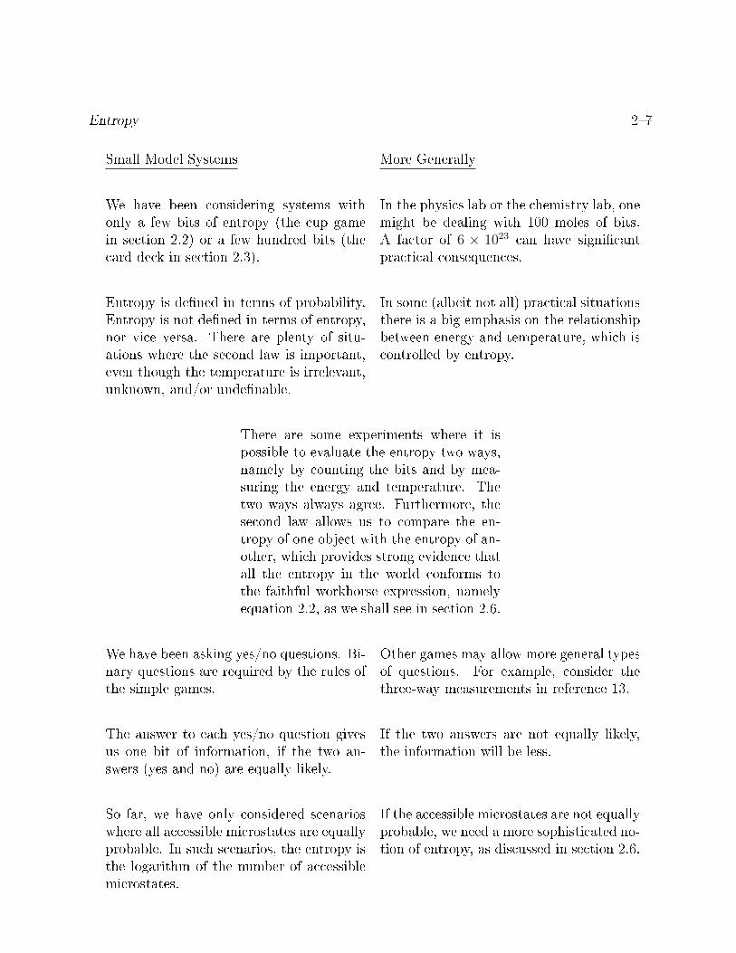
Entropy 27

Small Model Systems More Generally

We have been considering systems withonly a few bits of entropy (the cup gamein section 2.2) or a few hundred bits (thecard deck in section 2.3).

In the physics lab or the chemistry lab, onemight be dealing with 100 moles of bits.A factor of 6 × 1023 can have signicantpractical consequences.

Entropy is dened in terms of probability.Entropy is not dened in terms of entropy,nor vice versa. There are plenty of situ-ations where the second law is important,even though the temperature is irrelevant,unknown, and/or undenable.

In some (albeit not all) practical situationsthere is a big emphasis on the relationshipbetween energy and temperature, which iscontrolled by entropy.

There are some experiments where it ispossible to evaluate the entropy two ways,namely by counting the bits and by mea-suring the energy and temperature. Thetwo ways always agree. Furthermore, thesecond law allows us to compare the en-tropy of one object with the entropy of an-other, which provides strong evidence thatall the entropy in the world conforms tothe faithful workhorse expression, namelyequation 2.2, as we shall see in section 2.6.

We have been asking yes/no questions. Bi-nary questions are required by the rules ofthe simple games.

Other games may allow more general typesof questions. For example, consider thethree-way measurements in reference 13.

The answer to each yes/no question givesus one bit of information, if the two an-swers (yes and no) are equally likely.

If the two answers are not equally likely,the information will be less.

So far, we have only considered scenarioswhere all accessible microstates are equallyprobable. In such scenarios, the entropy isthe logarithm of the number of accessiblemicrostates.

If the accessible microstates are not equallyprobable, we need a more sophisticated no-tion of entropy, as discussed in section 2.6.


Remark on terminology: Any microstatesthat have appreciable probability are clas-sied as accessible. In contrast, mi-crostates that have negligible probabilityare classied as inaccessible. Their proba-bility doesn't have to be zero, just smallenough that it can be ignored withoutcausing too much damage.

Thermodynamics is a very practical sub-ject. It is much more common for someprobability to be negligible than to bestrictly zero.

In order to identify the correct microstatewith condence, we need to ask a sucientnumber of questions, so that the informa-tion contained in the answers is greaterthan or equal to the entropy of the game.

2.5.2 States and Probabilities

If you want to understand entropy, you must rst have at least a modest understanding ofbasic probability. It's a prerequisite, and there's no way of getting around it. Anyone whoknows about probability can learn about entropy. Anyone who doesn't, can't.

Our notion of entropy is completely dependent on having a notion of microstate, and onhaving a procedure for assigning a probability to each microstate.

In some special cases, the procedure involves little more than counting the accessi-ble (aka allowed) microstates, as discussed in section 9.6. This type of countingcorresponds to a particularly simple, at probability distribution, which may bea satisfactory approximation in special cases, but is denitely not adequate forthe general case.

For simplicity, the cup game and the card game were arranged to embody a clear notion ofmicrostate. That is, the rules of the game specied what situations would be considered thesame microstate and what would be considered dierent microstates. Note the contrast:

Entropy 29

Our discrete games provide a model that isdirectly and precisely applicable to physi-cal systems where the physics is naturallydiscrete, such as systems involving only thenonclassical spin of elementary particles.An important example is the demagnetiza-tion refrigerator discussed in section 11.10.

For systems involving continuous variablessuch as position and momentum, countingthe states is somewhat trickier ... but itcan be done. The correct procedure is dis-cussed in section 12.3.

For additional discussion of the relevance of entropy, as applied to thermodynamics andbeyond, see chapter 22.

2.5.3 Entropy is Not Knowing

The point of all this is that the score in these games is an example of entropy. Specically:at each point in the game, there are two numbers worth keeping track of: the number ofquestions we have already asked, and the number of questions we must ask to nish thegame. The latter is what we call the the entropy of the situation at that point.

Entropy is not knowing.Entropy measures how much is not known about the situation.

Remember that the macrostate is the ensemble of microstates. In the ensemble, probabilitiesare assigned taking into account what the observer knows about the situation. The entropyis a property of the macrostate.

At each point during the game, the entropy is a property of the macrostate, not of themicrostate. The system must be in some microstate, but generally we don't know whichmicrostate, so all our decisions must be based on the macrostate.

The value any given observer assigns to the entropy depends on what that observer knowsabout the situation, not what the dealer knows, or what anybody else knows. This makes theentropy somewhat context-dependent. Indeed, it is somewhat subjective. Some people ndthis irksome or even shocking, but it is real physics. For a discussion of context-dependententropy, see section 12.8.

2.5.4 Entropy versus Energy

Note that entropy has been dened without reference to temperature and without referenceto heat. Room temperature is equivalent to zero temperature for purposes of the cup gameand the card game. Arguably, in theory, there is some chance that thermal agitation willcause two of the cards to spontaneously hop up and exchange places during the game, butthat is really, really negligible.


Non-experts often try to dene entropy in terms of energy. This is a mistake. To calculatethe entropy, I don't need to know anything about energy; all I need to know is the probabilityof each relevant state. See section 2.6 for details on this.

States are states;they are not energy states.

Entropy is not dened in terms of energy, nor vice versa.

In some cases, there is a simple mapping that allows us to identify the ith microstate bymeans of its energy Ei. It is often convenient to exploit this mapping when it exists, but itdoes not always exist.

2.5.5 Entropy versus Disorder

In pop culture, entropy is often associated with disorder. There are even some textbooksthat try to explain entropy in terms of disorder. This is not a good idea. It is all themore disruptive because it is in some sense half true, which means it might pass supercialscrutiny. However, science is not based on half-truths.

Small disorder generally implies small entropy. However, the converse does not hold, noteven approximately; A highly-disordered system might or might not have high entropy. Thespin echo experiment (section 11.7) suces as an example of a highly disordered macrostatewith relatively low entropy.

Before we go any farther, we should emphasize again that entropy is a property of themacrostate, not of the microstate. In contrast, to the extent that disorder has any denitemeaning at all, it is a property of the microstate. Therefore, whatever the disorder ismeasuring, it isn't entropy. (A similar microstate versus macrostate argument applies to theenergy dispersal model of entropy, as discussed in section 9.8.) As a consequence, the usualtextbook illustration contrasting snapshots of orderly and disorderly scenes cannot bedirectly interpreted in terms of entropy. To get any scrap of value out of such an illustration,the reader must make a sophisticated leap:

The disorderly snapshot must be inter-preted as representative of an ensemblewith a very great number of similarly-disorderly microstates. The ensemble ofdisorderly microstates has high entropy.This is a property of the ensemble, not ofthe depicted microstate or any other mi-crostate.

The orderly snapshot must be interpretedas representative of a very small ensemble,namely the ensemble of similarly-orderlymicrostates. This small ensemble has asmall entropy. Again, entropy is a prop-erty of the ensemble, not of any particu-lar microstate (except in the extreme casewhere there is only one microstate in theensemble, and therefore zero entropy).

Entropy 211

To repeat: Entropy is dened as a weighted average over all microstates. Asking about theentropy of a particular microstate (disordered or otherwise) is asking the wrong question. Ifyou know what microstate the system is in, the entropy is zero. Guaranteed.

Note the following contrast:Entropy is a property of the macrostate. Itis dened as an ensemble average.

Disorder, to the extent it can be denedat all, is a property of the microstate.(You might be better o focusing on thesurprisal rather than the disorder, as dis-cussed in section 2.7.1.)

The number of orderly microstates is very small compared to the number of disorderlymicrostates. That's because when you say the system is ordered you are placing constraintson it. Therefore if you know that the system is in one of those orderly microstates, you knowthe entropy cannot be very large.

The converse does not hold. If you know that the system is in some disorderly microstate,you do not know that the entropy is large. Indeed, if you know that the system is in someparticular disorderly microstate, the entropy is zero. (This is a corollary of the more generalproposition that if you know what microstate the system is in, the entropy is zero. it doesn'tmatter whether that state looks disorderly or not.)

Furthermore, there are additional reasons why the typical text-book illustration of a messydorm room is not a good model of entropy. For starters, it provides no easy way to deneand delimit the states. Even if we stipulate that the tidy state is unique, we still don't knowhow many untidy states there are. We don't know to what extent a shirt on the oor here isdierent from a shirt on the oor there. Since we don't know how many dierent disorderlystates there are, we can't quantify the entropy. (In contrast the games in section 2.2 andsection 2.3 included a clear rule for dening and delimiting the states.)

Examples of low entropy and relatively high disorder include, in order of increasing com-plexity:

1. Quantum mechanical zero-point motion of a particle, such as the electron in a hydrogenatom. The electron is spread out over a nonzero area in phase space. It is spread ina random, disorderly way. However, the electron conguration is in a single, knownquantum state, so it has zero entropy.

2. Five coins in a known microstate.

Technical note: There is a separation of variables, analogous to the separation described in section 2.3.

We consider only the part of the system that describes whether the coins are in the heads or tails

state. We assume this subsystem is statistically independent of the other variables such as the position of

the coins, rotation in the plane, et cetera. This means we can understand the entropy of this subsystem

separately from the rest of the system, for reasons discussed in section 2.8.


Randomize the coins by shaking. The entropy at this point is ve bits. If you open thebox and peek at the coins, the entropy goes to zero. This makes it clear that entropyis a property of the ensemble, not a property of the microstate. Peeking does notchange the disorder. Peeking does not change the microstate. However, it can (andusually does) change the entropy. This example has the pedagogical advantage that itis small enough that the entire microstate-space can be explicitly displayed; there areonly 32 = 25 microstates.

3. A deck of cards in a known microstate.

Ordinarily, a well-shued deck of cards contains 225.581 bits of entropy, as discussedin section 2.3. On the other hand, if you have peeked at all the cards after they wereshued, the entropy is now zero, as discussed in section 2.4. Again, this makes it clearthat entropy is a property of the ensemble, not a property of the microstate. Peekingdoes not change the disorder. Peeking does not change the microstate. However, itcan (and usually does) change the entropy.

Many tricks of the card-sharp and the magic show illusionist depend on a deck ofcards arranged to have much disorder but little entropy.

4. In cryptography, suppose we have a brand-new one time pad containing a millionrandom hex digits. From our adversary's point of view, this embodies 4,000,000 bits ofentropy. If, however, the adversary manages to make a copy of our one time pad, thenthe entropy of our pad, from his point of view, goes to zero. All of the complexity isstill there, all of the disorder is still there, but the entropy is gone.

5. The spin echo experiment involves a highly complicated state that has low entropy.See section 11.7. This is a powerful example, because it involve a macroscopic amountof entropy. For a reasonable-sized sample, the total entropy could be on the order of1 joule per kelvin, i.e. on the order of 1023 bits, not just a few bits or a few hundredbits).

2.5.6 False Dichotomy, or Not

There is a long-running holy war between those who try to dene entropy in terms of energy,and those who try to dene it in terms of disorder. This is based on a grotesquely falsedichotomy: If entropy-as-energy is imperfect, then entropy-as-disorder must be perfect . . .or vice versa. I don't know whether to laugh or cry when I see this. Actually, both versionsare highly imperfect. You might get away with using one or the other in selected situations,but not in general.

The right way to dene entropy is in terms of probability, as we now discuss. (The variousother notions can then be understood as special cases and/or approximations to the trueentropy.)

Entropy 213

2.5.7 dQ, or Not

We do not dene entropy via dS = dQ/T or anything like that, for multiple reasons. Forone thing, as discussed in section 8.2, there is no state-function Q such that dQ = TdS (withperhaps trivial exceptions). Even more importantly, we need entropy to be well dened evenwhen the temperature is unknown, undened, irrelevant, or zero.

In the cup game (section 2.2) and in the card game (section 2.3), the temperature isirrelevant and eectively zero.

In the three-state system with a population inversion (section 11.4), the temperatureis undened and undenable.

2.6 Quantifying Entropy

The idea of entropy set forth in the preceding examples can be quantied quite precisely.Entropy is dened in terms of probability.1 For any classical probability distribution P , wecan dene its entropy as:

S[P ] :=∑i

Pi log(1/Pi) (2.2)

where the sum runs over all possible outcomes and Pi is the probability of the ith outcome.Here we write S[P ] to make it explicit that S is a functional that depends on P . For example,if P is a conditional probability then S will be a conditional entropy. Beware that peoplecommonly write simply S, leaving unstated the crucial dependence on P .

Equation 2.2 is the faithful workhorse formula for calculating the entropy. It ranks slightlybelow Equation 27.6, which is a more general way of expressing the same idea. It ranksabove various less-general formulas that may be useful under more-restrictive conditions(as in section 9.6 for example). See chapter 22 and chapter 27 for more discussion of therelevance and range of validity of this expression.

Subject to mild restrictions, equation 2.2 applies to physics as follows: Suppose the systemis in a given macrostate, and the macrostate is well described by a distribution P , where Piis the probability that the system is in the ith microstate. Then we can say S is the entropyof the system.

Expressions of this form date back to Boltzmann (reference 14 and reference 15)and to Gibbs (reference 16). The range of applicability was greatly expanded byShannon (reference 17). See also equation 27.6.

1Usually classical probability suces, as discussed in section 2.6, but if you really want the most generalformulation, the quantum statistics version is discussed in chapter 27.


Beware that uncritical reliance on the observed microstate-by-microstate probabilities doesnot always give a full description of the macrostate, because the Pi might be correlated withsomething else (as in section 11.7) or amongst themselves (as in chapter 27). In such casesthe unconditional entropy S[P ] will be larger than the conditional entropy S[P |Q], and youhave to decide which is/are physically relevant.

In the games discussed above, it was convenient to measure entropy in bits, because we wereasking yes/no questions. Other units are possible, as discussed in section 9.5.

Figure 2.2 shows the contribution to the entropy from one term in the sum in equation 2.2.Its maximum value is approximately 0.53 bits, attained when P (H) = 1/e.

0 0.2 0.4 0.6 0.8 1

P(H)

0

0.2

0.4

0.6

0.8

1

-P(H

) lo

g2

P(H

)

Figure 2.2: - P (H) log2 P (H) One Term in the Sum

Let us now restrict attention to a system that only has two microstates, such as a cointoss, so there will be exactly two terms in the sum. That means we can identify P (H) asthe probability of the the heads state. The other state, the tails state, necessarily hasprobability P (T) ≡ 1− P (H) and that gives us the other term in the sum, as shown by thered curve in gure 2.3. The total entropy is shown by the black curve in gure 2.3. For atwo-state system, it is necessarily a symmetric function of P (H). Its maximum value is 1bit, attained when P (H) = P (T) = 1/2.

The base of the logarithm in equation 2.2 is chosen according to what units you wish to use

Entropy 215

0 0.2 0.4 0.6 0.8 1

P(H)

0

0.2

0.4

0.6

0.8

1

-P(H

) lo

g2

P(H

) -

P(T

) lo

g2

P(T

)

Figure 2.3: Total Entropy Two-State System


for measuring entropy. Alternatively, as discussed in section 9.5, you can x the base of thelogarithm and stick in a prefactor that has some numerical value and some units:

S = −k∑i

Pi ln Pi (2.3)

Entropy itself is conventionally represented by big S. Meanwhile, molar entropy is conven-tionally represented by small s and is the corresponding intensive property.

People commonly think of entropy as being an extensive quantity. This is true to an excellentapproximation in typical situations, but there are occasional exceptions. Some exceptionsare discussed in section 12.8 and especially section 12.11.

Although it is often convenient to measure molar entropy in units of J/K/mol, other unitsare allowed, for the same reason that mileage is called mileage even when it is measuredin metric units. In particular, sometimes additional insight is gained by measuring molarentropy in units of bits per particle. See section 9.5 for more discussion of units.

When discussing a chemical reaction using a formula such as

2O3 → 3O2 + ∆s (2.4)

it is common to speak of the entropy of the reaction but properly it is the molar entropyof the reaction and should be written ∆s or ∆S/N (not ∆S). All the other terms in theformula are intensive, so the entropy-related term must be intensive also.

Of particular interest is the standard molar entropy, s i.e. S/N , measured at standard tem-perature and pressure. The entropy of a gas is strongly dependent on density, as mentionedin section 12.3.

2.7 Microstate versus Macrostate

2.7.1 Surprisal

If we have a system characterized by a probability distribution P , the surprisal of the ithmicrostate is given by

$i := log(1/Pi) (2.5)

By comparing this with equation 2.2, it is easy to see that the entropy is simply the ensembleaverage of the surprisal. In particular, it is the expectation value of the surprisal. (Seeequation 27.7 for the fully quantum-mechanical generalization of this idea.)

Entropy 217

2.7.2 Contrasts and Consequences

Note the following contrast: For any given microstate i and any given distribution P :

Surprisal is a property of the microstate i. Entropy is a property of the distributionP as a whole. It is dened as an ensembleaverage.

Entropy is a property of the macrostatenot of the microstate.

A manifestation of this can be seen in item 4.

When you hear that entropy is a property of the distribution, the word the shouldnot receive undue emphasis. The complete assertion says that for any given distribution

the entropy is a property of the distribution, and the second half must not be taken out ofcontext. There are lots of dierent distributions in this world, and you should not thinkin terms of the one true distribution. Indeed, it is common to deal with two or moredistributions at the same time.

Given just a microstate, you do not know what distribution it was drawn from. For example,consider the point at the center of the small black circle in gure 2.4. The point itself hasno uncertainty, no width, no error bars, and no entropy. The point could have been drawnfrom the red distribution or the blue distribution; you have no way of knowing. The entropyof the red distribution is clearly dierent from the entropy of the blue distribution.

In a card came such as poker or go sh, it is common for dierent players to use dierentmacrostates (dierent distributions), even though the microstate (the objective state of thecards) is the same for all, as discussed in section 2.4. Ditto for the game of Clue, or anyother game of imperfect information. Similarly, in cryptography the sender and the attackervirtually always use dierent distributions over plaintexts and keys. The microstate is knownto the sender, whereas the attacker presumably has to guess. The microstate is the same forboth, but the macrostate is dierent.

Another obvious consequence of equation 2.5 is that entropy is not, by itself, the solutionto all the world's problems. Entropy measures a particular average property of the givendistribution. It is easy to nd situations where other properties of the distribution are worthknowing. The mean, the standard deviation, the entropy, various Rényi functionals, etc. arejust a few of the many properties. (Note that the Rényi functionals (one of which is just theentropy) can be dened even in situations where the mean and standard deviation cannot,e.g. for a distribution over non-numerical symbols.)

For more about the terminology of state, microstate, and macrostate, see section 12.1.


0 5 10 15 20 250.00

0.05

0.10

0.15

0.20

Figure 2.4: One Point, Two Distributions

2.8 Entropy of Independent Subsystems

Suppose we have subsystem 1 with a set of microstates (i) and subsystem 2 with a set ofmicrostates (j). Then in all generality, the microstates of the combined system are givenby the direct product of these two sets, namely

(i) × (j) = (i, j) (2.6)

where (i, j) is an ordered pair, which should be a familiar idea and a familiar notation. Weuse × to denote the Cartesian direct product.

We now restrict attention to the less-than-general case where the two subsystems are statis-tically independent. That means that the probabilities are multiplicative:

R(i, j) = P (i)Q(j) (2.7)

Let's evaluate the entropy of the combined system:S[R] = −

∑i,j R(i, j) log[R(i, j)]

= −∑

i,j P (i)Q(j) log[P (i)Q(j)]

= −∑

i,j P (i)Q(j) log[P (i)]−∑

i,j P (i)Q(j) log[Q(j)]

= −∑

j Q(j)∑

i P (i) log[P (i)]−∑

i P (i)∑

j Q(j) log[Q(j)]

= S[P ] + S[Q]

(2.8)

where we have used the fact that the subsystem probabilities are normalized.

So we see that the entropy is additive whenever the probabilities are multiplicative, i.e.whenever the probabilities are independent.

Chapter 3

Basic Concepts (Zeroth Law)

There are a bunch of basic notions that are often lumped together and called the zerothlaw of thermodynamics. These notions are incomparably less fundamental than the notionof energy (the rst law) and entropy (the second law), so despite its name, the zeroth lawdoesn't deserve priority.

Here are some oft-cited rules, and some comments on each.

We can divide the world into some numberof regions that are disjoint from each other.

If there are only two regions, some peoplelike to call one of them the system andcall the other the environment, but usu-ally it is better to consider all regions onan equal footing. Regions are sometimescalled systems, or subsystems, or zones, orparcels. They are sometimes called objects,especially when they are relatively simple.

There is such a thing as thermal equilib-

rium.You must not assume that everything isin thermal equilibrium. Thermodynamicsand indeed life itself depend on the factthat some regions are out of equilibriumwith other regions.

There is such a thing as temperature. There are innumerable important exam-ples of systems that lack a well-denedtemperature, such as the three-state laserdiscussed in section 11.4.


Whenever any two systems are in equi-librium with each other, and they eachhave a well-dened temperature, then thetwo temperatures are the same. See sec-tion 10.1 and chapter 23.

This is true and important. (To be pre-cise, we should say they have the same av-erage temperature, since there will be uc-tuations, which may be signicant for verysmall systems.)

Equilibrium is transitive. That is, if A is inequilibrium with B and B is in equilibriumwith C, then A is in equilibrium with C.See chapter 23.

This not always true. To understand howit sometimes goes wrong, we must keep inmind that there are dierent types of equi-librium. If A equilibrates with B by ex-change of electrons and B equilibrates withC by exchange of ions, interesting thingscan happen. In particular, we can build abattery. When the battery is sitting thereopen-circuited, all of the components areessentially in equilibrium ... local pairwiseequilibrium ... but the two terminals arenot in equilibrium, as you will discover ifyou wire up a load.

We can establish equilibrium within asystem, and equilibrium between selectedpairs of systems, without establishing equi-librium between all systems.

This is an entirely nontrivial statement.Sometimes it takes a good bit of engineer-ing to keep some pairs near equilibriumand other pairs far from equilibrium. Seesection 11.11.

If/when we have established equilibriumwithin a system, a few variables suce toentirely describe the thermodynamic state

(i.e. macrostate) of the system.1 (See sec-tion 2.7 and section 12.1 for a discussion ofmicrostate versus macrostate.)

This is an entirely nontrivial statement,and to make it useful you have to be cageyabout what variables you choose; for in-stance:

Basic Concepts (Zeroth Law) 33

• Knowing the temperature and pres-sure of a parcel of ice gives you more-or-less a complete description of thethermodynamic state of the ice.• Knowing the temperature and pres-sure of a parcel of liquid water givesyou more-or-less a complete descrip-tion of the thermodynamic state ofthe water.• Meanwhile, in contrast, knowingthe temperature and pressure of anice/water mixture does not fully de-termine the thermodynamic state,because you don't know what frac-tion is ice and what fraction is water.

In addition to all these thermo-related concepts, we must also comply with all the non-thermal laws of physics, including conservation of momentum, conservation of charge, etcetera. This is discussed in chapter 5.

Chapter 4

Low-Temperature Entropy (AllegedThird Law)

As mentioned in the introduction, one sometimes hears the assertion that the entropy of asystem must go to zero as the temperature goes to zero.

There is no theoretical basis for this assertion, so far as I know just unsubstantiated opinion.

As for experimental evidence, I know of only one case where (if I work hard enough) I canmake this statement true, while there are innumerable cases where it is not true:

• There is such a thing as a spin glass. It is a solid, with a spin at every site. At lowtemperatures, these spins are not lined up; they are highly disordered. And thereis a large potential barrier that prevents the spins from ipping. So for all practicalpurposes, the entropy of these spins is frozen in. The molar entropy involved is sub-stantial, on the order of one J/K/mole. You can calculate the amount of entropy basedon measurements of the magnetic properties.

• A chunk of ordinary glass (e.g. window glass) has a considerable amount of frozen-inentropy, due to the disorderly spatial arrangement of the glass molecules. That is,glass is not a perfect crystal. Again, the molar entropy is quite substantial. It can bemeasured by X-ray scattering and neutron scattering experiments.

• For that matter, it is proverbial that perfect crystals do not occur in nature. Thisis because it is energetically more favorable for a crystal to grow at a dislocation.Furthermore, the materials from which the crystal was grown will have chemical im-purities, not to mention a mixture of isotopes. So any real crystal will have frozen-innonuniformities. The molar entropy might be rather less than one J/K/mole, but itwon't be zero.

• If I wanted to create a sample where the entropy went to zero in the limit of zerotemperature, I would proceed as follows: Start with a sample of helium. Cool it tosome very low temperature. The superuid fraction is a single quantum state, so it


has zero entropy. But the sample as a whole still has nonzero entropy, because 3He isquite soluble in 4He (about 6% at zero temperature), and there will always be some3He around. To get rid of that, pump the sample through a superleak, so the 3He isleft behind. (Call it reverse osmosis if you like.) Repeat this as a function of T . As Tgoes to zero, the superuid fraction goes to 100% (i.e. the normal-uid fraction goesto 0%) so the entropy, as far as I know, would go to zero asymptotically.

Note: It is hard to measure the low-temperature entropy by means of elementary thermalmeasurements, because typically such measurements are insensitive to spectator entropy asdiscussed in section 12.6. So for typical classical thermodynamic purposes, it doesn't matterwhether the entropy goes to zero or not.

Chapter 5

The Rest of Physics, Chemistry, etc.

The previous sections have set forth the conventional laws of thermodynamics, cleaned upand modernized as much as possible.

At this point you may be asking, why do these laws call attention to conservation of energy,but not the other great conservation laws (momentum, electrical charge, lepton number, etcetera)? And for that matter, what about all the other physical laws, the ones that aren'texpressed as conservation laws? Well, you're right, there are some quite silly inconsistencieshere.

The fact of the matter is that in order to do thermo, you need to import a great deal ofclassical mechanics. You can think of this as the minus-oneth law of thermodynamics.• This includes Newton's third law (which is tantamount to conservation of momentum)and Newton's second law, with the associated ideas of force, mass, acceleration, etcetera. Note that the concept of pseudowork, which shows up in some thermodynamicdiscussions, is more closely related to the momentum and kinetic energy than it is tothe total energy.• In particular, this includes the notion of conservation of energy, which is a well-established part of nonthermal classical mechanics. From this we conclude that therst law of thermodynamics is redundant and should, logically, be left unsaid (althoughit remains true and important).• If you are going to apply thermodynamics to a chemical system, you need to import thefundamental notions of chemistry. This includes the notion that atoms exist and areunchanged by ordinary chemical reactions (which merely denes what we mean by achemical as opposed to nuclear reaction). This implies about a hundred additionalapproximate1 conservation laws, one for each type of atom. The familiar practice ofbalancing the reaction equation is nothing more than an application of these atom-conservation laws.

1Subject to the approximation that nuclear reactions can be neglected.


• If you are going to apply thermodynamics to an electrical or magnetic system, youneed to import the laws of electromagnetism, i.e. the Maxwell equations.• The Maxwell equations imply conservation of charge. This is essential to chemistry,in the context of redox reactions. It means you have to balance the reaction equationwith respect to charge. This is in addition to the requirement to balance the reactionequation with respect to atoms.

Sometimes the process of importing a classical idea into the world of thermodynamics istrivial, and sometimes not. For example:

The law of conservation of momentumwould be automatically valid if we appliedit by breaking a complex object into its el-ementary components, applying the law toeach component separately, and summingthe various contributions. That's ne, butnobody wants to do it that way. In thespirit of thermodynamics, we would prefera macroscopic law. That is, we would liketo be able to measure the overall mass ofthe object (M), measure its average veloc-ity (V ), and from that compute a macro-scopic momentum (MV ) obeying the lawof conservation of momentum. In fact thismacroscopic approach works ne, and canfairly easily be proven to be consistent withthe microscopic approach. No problem.

The notion of kinetic energy causes troublewhen we try to import it. Sometimes youwant a microscopic accounting of kineticenergy, and sometimes you want to includeonly the macroscopic kinetic energy. Thereis nontrivial ambiguity here, as discussedin section 18.4 and reference 18.

Chapter 6

Classical Thermodynamics

6.1 Overview

So far we have discussed only a few basic ideas, but already we know enough to handle someinteresting applications.

6.2 Stirling Engine

6.2.1 Basic Structure and Operations

Let's consider a Stirling engine. This is a type of heat engine; that is, it takes in energy andentropy via one side, dumps out waste energy and entropy via the other side, and performsuseful work via a crankshaft.

In operation, the Stirling engine goes through a cycle of four states A,B,C,D connectedby four legs AB,BC,CD,DA. The Stirling cycle is rectangle in (T, V ) space, as shownin gure 6.1.

There are many ways of building a Stirling engine. The ones that are easy to build are noteasy to analyze. (Actually all Stirling engines are infamously hard to analyze.) Let's consideran idealized version. One way of carrying out the volume-changes called for in gure 6.1 isshown in gure 6.2. You can see that there are two cylinders: an always-hot cylinder at theleft, and an always-cold cylinder at the right. Each cylinder is tted with a piston. Whenwe speak of the volume, we are referring to the combined volume in the two cylinders.


copyright © 2015 jsd

Temperature

Volume

A

BC

D

AB

BC

CD

DA

Figure 6.1: Stirling Cycle

Classical Thermodynamics 63

warming at constant small volume

compression at constant low temperature

cooling at constant large volume

expansion at constant high temperature


V = 1

V = 1

V = 3

V = 3

V = 1A

B

C

D

A

AB

BC

CD

DA

Figure 6.2: Stirling Engine : Volume Changes


Cooling

Let's now examine the required temperature-changes. Figure 6.3 shows a more completepicture of the apparatus. In addition to the two cylinders, there is also a thin tube allowingthe working uid to ow from the hot side to the cold side and back again.

cooling at constant large volume


Figure 6.3: Stirling Engine : Cooling Phase

Figure 6.3 shows a snapshot taken during the cooling phase, i.e. the BC leg. The two pistonsmove together in lock-step, so the total volume of uid remains constant. As the uid owsthrough the tube, it encounters a series of heat exchangers. Each one is a little cooler thanthe next. At each point, the uid is a little bit warmer than the local heat exchanger, so it


gives up a little bit of energy and entropy. At each point the temperature dierence is small,so the transfer is very nearly reversible. We idealize it as completely reversible.

Warming

warming at constant small volume


Figure 6.4: Stirling Engine : Warming Phase

Figure 6.4 shows a snapshot taken during the warming phase, i.e. the DA leg. Once again,the two pistons move together in lock-step, so the total volume of uid remains constant.The volume here is less than the volume during the cooling phase, so each piston moves less,but still they force all the volume to ow through the tube. (If you're clever, you can arrange


that the pistons move with less velocity during this leg, so that the overall time is the samefor both the DA leg and the BC leg. That is, you can arrange that the ow rate in molesper second is the same, even though the ow rate in cubic meters per second is dierent.This gives the heat exchangers time to do their job.)

As the uid ows through the tube, it encounters the same series of heat exchangers, inreverse order. At each point, the uid is a little bit cooler than the local heat exchanger,so it picks up a little bit of energy and entropy. At each point the temperature dierence issmall, so the transfer is very nearly reversible. We idealize it as completely reversible.

The same number of moles of uid underwent the same change of temperature, in the oppositedirection, so the energy and entropy involved in the DA leg are equal-and-opposite to theenergy and entropy involved in the BC leg. The molar heat capacity at constant volume isa constant, independent of density, for any ideal gas (or indeed any polytropic gas).

It must be emphasized that during the BC leg and also during the DA leg, no energy orentropy leaves the system. No energy or entropy crosses the dotted-line boundary shown inthe diagram. The heat exchangers arrayed along the thin tube are strictly internal to thesystem. They do not require fuel or coolant from outside. They are like little cookie jars;you can put cookies and and take cookies out, but they do not produce or consume cookies.At the end of each cycle, they return to their original state.

Expansion

Figure 6.5 shows the expansion phase. The uid is all on the hot side of the machine. Thepiston is retreating, so the uid expands. If it were allowed to expand at constant entropy,it would cool, but we do not allow that. Instead we supply energy from an external source,to maintain the uid at a constant temperature as it expands.

Compression

Figure 6.6 shows the compression phase. The uid is all on the cold side of the machine. Thecold piston is advancing, so the uid is compressed into a smaller volume. If it were com-pressed at constant entropy, it would warm up, but we do not allow that. Instead we supplysupply cooling from an external source, to maintain the uid at a constant temperatureduring the compression.

6.2.2 Energy, Entropy, and Eciency

It must be emphasized that the source that supplies energy and entropy on the left side ofgure 6.5 is in a completely dierent category from the cookie jars attached to the ow tube.


expansion at constant high temperature


hotbath

required

∞

Figure 6.5: Stirling Engine : Expansion Phase


compression at constant low temperature


coldbath

required

∞

Figure 6.6: Stirling Engine : Compression Phase


The source provides energy and entropy that ow across the boundary of the system. Weimagine that the external high-side heat bath has an innite heat capacity, so that we canextract energy and entropy from it without changing its temperature.

Similar words apply to the cooling system on the right side of gure 6.6. This is in acompletely dierent category from the cookie jars, because energy and entropy are crossingthe boundary of the system. We imagine that the low-side heat bath has an innite heatcapacity, so that we can dump energy and entropy into it without changing its temperature.

To summarize: Legs AB and CD are in one category (energy and entropy crossing theboundary, cumulatively, without end) while BC and DA are in another category (energyand entropy being rearranged interneally, with no net change from cycle to cycle).

The diagrams in this section do not show the crankshaft that delivers useful work to theoutside. However we can easily enough gure out how much work is involved.

No work is performed on the BC leg or on the DA leg. The volume is the same before andafter, so there is no PdV work. We are assuming an ideal engine, so the pressure on bothsides is the same. The pressure changes during the BC leg (and during the DA leg), but ateach instant the pressure at both ends of the machine is the same.

During the AB leg the volume increases by a certain amount, and then on the CD leg thevolume decreases by the same amount. We know the uid is hotter on the AB leg, so it hasa higher pressure, so there is a net amount of PdV work done. For an ideal gas, it is easy todo the integral PdV . You don't even need to assume a monatomic gas; a polyatomic idealgas such as air is just as easy to handle. A factor of T comes out in front of the integral.

So, on a per-cycle basis, the energy that comes in on the left is proportional to Thot, whilethe energy that goes out on the right is proportional to Tcold.

We dene the eciency of a heat engine as

ηhe :=mechanical energy out

energy in (for any heat engine) (6.1)

so for this particular heat engine, given all our idealizations, the eciency is

ηhe :=Thot−Tcold

Thot(for an ideal Stirling engine) (6.2)

6.2.3 Practical Considerations; Temperature Match or Mismatch

Note that each hardware component in a Stirling engine sits at more-or-less steady tem-perature over time. The working uid changes temperature signicantly, but the hardwarecomponents do not. Increasing the thermal contact between the hardware and the uid (atany given point) makes the engine work better. (On the other hand, we need to minimizethermal conduction between one cookie jar and the next, in the regenerator.)


A gas turbine engine (such as you nd on a jet aircraft) is similar, insofar as the uid changestemperature, while the hardware components do not, to any great extent. Also, the workinguid never comes in contact with hardware that is at a signicantly dierent temperature.It is however in a dierent subcategory, in that improving the contact between the workinguid and the hardware will not make the engine work better.

This stands in contrast to a Carnot cycle, which depends on heating up and cooling downthe cylinder that holds the working uid. This is of course possible in theory, but it istroublesome in practice. It tends to reduce the power density and/or the eciency of theengine. James Watt's rst steam engine suered from this problem to a serious degree. Itwas only later that he gured out the advantages of having a separate condenser.

In a third category we have piston engines of the kind that you nd in an ordinary automobileor lawn mower. They have the ugly property that the working uid comes into contact withhardware at wildly dissimilar temperatures. This limits the eciency, especially at lowspeeds. Making stronger contact between the working uid and the cylinder walls wouldmake the engine work worse. A similar temperature-mismatch problem occurs in the pistonsof an external-combustion piston engines, such as piston-type steam engine, because thesteam cools as it expands. (Of course a steam engine requires good thermal contact in theboiler and the condenser.)

6.2.4 Discussion: Reversibility

As discussed in section 7.1, under mild assumptions we can write

dE = −PdV + TdS (6.3)

We apply this to the heat baths that attach to the left and right side of our engine. Weconnect to the heat baths in such a way that we do not aect their pressure or volume, sowe have simply:

dE = TdS (at constant V ) (6.4)

Since for our engine, ∆E is proportional to temperature, we see that the amount of entropywe take in from the left is exactly the same as the amount of entropy we dump out on theright. (As always, it is assumed that no entropy ows out via the crankshaft.)

This property entropy in equals entropy out is the hallmark of a reversible engine. Anideal Stirling engine is reversible.

A heat engine operated in reverse serves as a heat pump. A household refrigerator is anexample: It pumps energy and entropy from inside the refrigerator to outside. Other heatpumps are used to provide heat for buildings in the winter.


6.3 All Reversible Heat Engines are Equally Ecient

We now consider the class of all devices that

1. are heat engines,

2. are reversible, and

3. run o a single hot bath (Thot) and a single cold bath (Tcold).

The claim is that all such engines are equally ecient.

The proof is stunningly simple and powerful: If you had two reversible heat engines withdierent eciencies, you could hook them in parallel and create a perpetual motion machine!

As a corollary: We know the eciency of all such devices (for any given pair of temperatures).

The proof is equally simple: Given that all devices that meet our three criteria are equallyecient, if you know the eciency of one, you know them all. And we do know the eciencyof one, so we in fact we know them all. This is called the Carnot eciency of a heat engine.It is:

ηhe :=Thot−Tcold

Thot(for any 2-bath reversible heat engine) (6.5)

As long as you are getting your energy from a heat bath, it is not possible to design anengine with greater eciency than this, no matter how clever you are.

This is the glory of classical thermodynamics. Sadi Carnot gured this out long before therewas a modern understanding of what energy is. The result depends on little more than thedenition of temperature. In fact, the result can be turned around to serve as an operationaldenition of temperature: If you have an object at some known reference temperature, andanother object at some unknown temperature, you can operate a reversible heat enginebetween the two, observe the eciency, and deduce a value for the previously-unknowntemperature.

Here's another way of understanding the universal eciency result. Imagine we have a heatengine that is reversible, but less ecient than we would expect based on equation 6.5. As aheat engine, it is less ecient, but as a heat pump it is more ecient! It is a too-good-to-be-true heat pump. As a heat pump, it takes in too much entropy on the cold side and ejectstoo little on the hot side. This violates the law of paraconservation of entropy (section 2.1).

6.4 Not Everything is a Heat Engine

It must be emphasized that the discussion in section 6.3 applies to heat engines and nototherwise. In particular, consider an electrochemical fuel cell. If it's done right, the eciency


of such a thing vastly exceeds 1 − Tcold/Thot. That's OK, because it's not a heat engine.Even though it takes in fuel and puts out work, it is not a heat engine.

As an even more familiar example, consider a plain old electrochemical battery driving anelectric motor. If it's done right, the eciency of such a thing vastly exceeds 1−Tcold/Thot.

It is not worth the trouble to try to understand such things in terms of heat, or in terms ofclassical thermodynamics generally. I doubt it is even possible.

It is however straightforward to understand such things in terms of modern (post-1898)thermodynamics, i.e. statistical mechanics. Rather than getting bogged down trying todene heat, formalize everything in terms of energy and entropy instead. Entropy is denedin terms of probability, as a sum over states. In a battery, the state that stores the energydoesn't even have a temperature, and it isn't in equilibrium with your thermometer.

Let's be clear: For a heat bath, its entropy is proportional to its energy, and the constant ofproportionality is the inverse temperature. For a battery, that's just not true. You can sticka lot of energy into a battery without changing its temperature.

6.5 Carnot Eciency Formula

We can derive a famous formula that places limits on the eciency of any so-called heat-engine.

6.5.1 Denition of Heat Engine

Figure 6.7 is a sketch of such an engine. The details don't matter. The key concept is thatthe heat engine, by denition, has three connections, highlighted by magental labels in thegure.

Even though this is called a heat engine, trying to quantify the heat is a losing strategy.It is simpler and in every way better to quantify the energy and the entropy.

We could write the change in the energy content of the engine using equation 6.6, includingall the terms on the RHS. However, as part of our denition of what we mean by heat engine,we require that only the terms shown in magenta are signicant.

dE = T3dS3 − F3 · dX3 + · · · (connection #3)+ T2dS2−F2 · dX2 + · · · (connection #2)+ T1dS1 − F1 · dX1 + · · · (connection #1)

(6.6)

More specically, we require that connection #3 be 100% thermal, connection #2 be 100%mechanical i.e. nonthermal, and connection #1 be 100% thermal. The engine is designed tosegregate the thermal energy-transfers from the mechanical energy-transfers.


dS1

T1

dS3

T3

•dX2

F2

Figure 6.7: Heat Engine


We have just constructed a theoretical model of an engine. This is a remarkbly good modelfor a wide range of real-world engines. However, it must be emphasized that it does notapply to all engines. In particular, it does not apply to batteries or to electrochemical fuelcells.

We must impose one more restriction: We require that the engine be able to operate in acycle, such that at the end of the cycle, after doing something useful, all the internal parts ofthe engine return to their initial state. In particular, we require that the engine not have ahollow leg where it can hide unlimited amounts of entropy for unlimited amounts of time.This requirement makes sense, because if entropy could be hidden, it would defeat the spiritof the second law of thermodynamics.

Without loss of generality we assume that T2 ≥ T1. There is no loss of generality, because theengine is symmetrical. If necessary, just relabel the connections to make T2 ≥ T1. Relabelingis just a paperwork exercise, and doesn't change the physics.

6.5.2 Analysis

The engine starts by taking in a certain amount of energy via connection #3. We mighthope to convert all of this heat-energy to useful work and ship it out via connection #2, butwe can't do that. The problem is that because connection #3 is a thermal connection, whenwe took in the energy, we also took in a bunch of entropy, and we need to get rid of thatsomehow. We can't get rid of it through connection #2, so the only option is to get rid ofit through connection #1.

For simplicity, we assume that T3 and T1 are constant throughout the cycle. We also makethe rather mild assumption that T1 is greater than zero. Section 6.5.3 discusses ways toloosen these requirements.

Under these conditions, pushing entropy out through connection #1 costs energy. We callthis the waste heat:

waste heat = −∫

ΓT1dS1 (6.7)

where the path Γ represents one cycle of operating the engine.

We can now use conservation of energy to calculate the mechanical work done by the engine:work out =

∫ΓF2 · dX2 (6.8a)

=∫

ΓT3dS3 +

∫ΓT1dS1 (6.8b)

= T3∆S3 + T1∆S1 (6.8c)

where on the last line we have used that fact that the temperatures are unchanging to allowus to do the entropy-integrals. The deltas implicitly depend on the path Γ.


The second law tells us that over the course of a cycle, the entropy going out via connection#1 (−∆S1) must be at least as much as the entropy coming in via connection #3 (+∆S3).For a reversible engine, the two are equal, and we can write:

∆S3 = +∆SI

∆S1 = −∆SI(6.9)

Where ∆SI is pronounced delta S through and denotes the amount of entropy that owsthrough the engine, in the course of one cycle. We dene the eciency as

η := mechanical transfer outthermal transfer in (6.10)

Still assuming the temperatures are greater than zero, the denominator in this expression isjust T3∆S3. Combining results, we obtain:

η := T3∆S3+T1∆S1

T3∆S3(6.11)

The maximum eciency is obtained for a thermodynamically reversible engine, in whichcase

ηrev = T3∆SI−T1∆SIT3∆SI

(6.12a)= T3−T1

T3(6.12b)

where equation 6.12b is the famous Carnot eciency formula, applicable to a reversibleheat engine. The meaning of the formula is perhaps easier to understand by looking atequation 6.12a or equation 6.11, wherein the second term in the numerator is just the wasteheat, in accordance with equation 6.7.

Let us now consider an irreversible engine. Dissipation within the engine will create extraentropy, which will have to be pushed out via connection #1. This increases the waste heat,and decreases the eciency η. In other words, equation 6.12b is the exact eciency for areversible heat engine, and an upper bound on the eciency for any heat engine.

6.5.3 Discussion

(1) If you were wondering whether it is possible to construct even one thermodynamic cyclethat complies with all the restrictions in section 6.5.2, fear not. The job can be doneusing a Carnot cycle, as described in section 8.7. On the other hand, as mentioned inthat section, the Carnot cycle often gets more attention than it deserves.

(2) Furthermore, the Carnot eciency formula often gets more attention than it deserves.

For one thing, not all engines are heat engines. The Carnot eciency formulaequation 6.12b applies only to heat engines, as dened by the magenta terms inequation 6.6.As a specic, important counterexample, a battery or an electrochemical fuel cellcan have an eciency enormously greater than what you would guess based onequation 6.12b ... even in situations where the chemicals used to run the fuel cellcould have been used to run a heat engine instead.


Consider the following scenario: Some guy buys a bunch of coal. He uses it toboil some steam at temperature T3. He uses that to drive a steam engine. Heuses river water to cool the condenser at temperature T1. He manages to operatethe engine in such a way that its eciency is close to the Carnot eciency. He isvery pleased with himself, and runs spots on television advertising how ecienthe is. I'm as ecient as the laws of physics allow, other things being equal.

The problem is, he's asking the wrong question. Rather than asking how well heis doing relative to the Carnot eciency, he should be asking how well he is doingrelative to the best that could be done using the same amount of fuel.

Specically, in this scenario, the guy next door is operating a similar engine, butat a higher temperature T3. This allows him to get more power out of his engine.His Carnot eciency is 30% higher. His actual eciency is only 20% higher,because there are some unfortunate parasitic losses. So this guy is not runningas close to the Carnot limit as the previous guy. Still, this guy is doing better inevery way that actually matters.

[This assumes that at least part of the goal is to minimize the amount of coalconsumed (for a given amount of useful work), which makes sense given that coalis a non-renewable resource. Similarly part of the goal is to minimize the amountof CO2 dumped into the atmosphere. The competing engines are assumed to havecomparable capital cost.]

Suppose you are trying to improve your engine. You are looking for ineciencies. Let'sbe clear: Carnot eciency tells you one place to look ... but it is absolutely not theonly place to look.

(3) Looking at the structure of the result in equation 6.12b, one can understand why wewere tempted to require that T1 and T3 have denite, constant values.

However, any heat engine still has a well-dened thermal eciency, as dened byequation 6.10, even if the temperatures are changing in peculiar ways over the courseof the cycle.

Furthermore, with some extra work, you can convince yourself that the integrals inequation 6.8b take the form of a ∆S times an average temperature. It's a peculiartype of weighted average. This allows us to interpret the Carnot eciency formula(equation 6.12b) in a more general, more exible way.

(4) As a slightly dierent line of reasoning that leads to the same conclusion, start withan ordinary Carnot cycle, such as we see in gure 8.5 or gure 8.6. You can imaginecovering the entire space with a mosaic of tiny Carnot cycles, as shown in gure 6.8.There is one big cycle made up of nine tiny cycles, such that the left edge of one cyclecoincides with the right edge of another, and the top of one coincides with the bottomof another. For an ideal reversible engine, going around each of the nine tiny cycles


once is identical to going around the big cycle once, because all of the interior edgescancel.

By selecting a suitable set of the tiny Carnot cycles, you can approximate a wide classof reversible cycles. The eciency can be calculated from the denition, equation 6.10,by summing the thermal and mechanical energy, summing over all the sub-cycles.

0 1 2 3 4 5 6

Volume

0.0

0.2

0.4

0.6

0.8

1.0

Temperature

Figure 6.8: Carnot Cycle with Sub-Cycles

(5) A hot gas has more entropy than a cool gas. This is partly because the probabilitydistribution is more spread out in phase space, more spread out along the momentumdirection. It is also partly because the unit of measure in phase space is smaller, asdiscussed in section 12.3.

Because of the higher entropy, you might think the gas has less available energy(whatever that means). However, the hot gas contains more energy as well as moreentropy, and it is easy to nd situations where the hot gas is more useful as an energy-source, for instance if the gas is applied to connection #3 in a heat engine. Indeed,in order to increase eciency in accordance with equation 6.12, engine designers arealways looking for ways to make the hot section of the engine run hotter, as hot aspossible consistent with reliability and longevity.

Of course, when we examine the cold side of the heat engine, i.e. connection #1, thenthe reverse is true: The colder the gas, the more valuable it is for producing usefulwork. This should make it clear that any notion of available energy cannot possiblybe a function of state. You cannot look at a bottle of gas and determine how much ofits energy is available not without knowing a whole lot of additional informationabout the way in which the gas is to be used. This is discussed in more detail insection 1.7.3.

(6) If you take equation 6.12b and mindlessly extrapolate it to the case where T1 is negative,you might hope to achieve an eciency greater than 100%. However, before doing thatnote that the dening property of negative temperature is that when entropy goes outvia connection #1, energy comes in. Therefore we must include this energy input in


the denominator in the denition of eciency, equation 6.10. When we do that, insteadof getting equation 6.11 we get:

η := T3∆S3+T1∆S1

T3∆S3+T1∆S1

= 100% (always)(6.13)

Both terms in the denominator here are positive; the second term involves a doublenegative.

We can understand this as follows: Whenever there are two thermal connections, one ata positive temperature and one at a negative temperature, the engine takes in energyvia both thermal connections, and sends it all out via the mechanical connection.Therefore the eciency is always exactly 100%, never more, never less.

Even if the engine is irreversible, such that −∆S1 is greater than −∆S3, the engineis still 100% ecient in its use of energy, because absolutely all of the energy that isthermally transferred in gets mechanically transferred out.

These conclusions are restricted to a model that assumes the engine has only threeconnections to the rest of the world. A more realistic engine model would allow foradditional connections; see next item.

(7) A term involving T4∆S4 could be added to our model, to represent losses due to friction,losses due to heat leaks, et cetera.

η := T3∆S3+T1∆S1+T4∆S4

T3∆S3+T1∆S1

< 100% (since T4∆S4 < 0)(6.14)

In the real world, the only known ways of producing a heat bath at negative temperatureare horrendously inecient, so the 100% eciency mentioned in the previous items isnowhere near being relevant to a complete, practical system.

Chapter 7

Functions of State

7.1 Functions of State : Basic Notions

Terminology: By denition, the term state function applies to any measurable quantity thatis uniquely determined by the thermodynamic state, i.e. the macrostate.

Terminology: The term thermodynamic potential is synonymous with state function. Alsothe term function of state is synonymous with state function.

Example: In an ordinary chunk of metal at equilibrium, state functions include energy (E),entropy (S), temperature (T ), molar volume (V/N), total mass, speed of sound, et cetera.Some additional important thermodynamic potentials are discussed in chapter 15.

In thermodynamics, we usually arrange for the energy E to be a function of state. Thisdoesn't tell us anything about E, but it tells us something about our notion of thermo-dynamic state. That is, we choose our notion of state so that E will be a function ofstate.

Similarly, we usually arrange for the entropy S to be a function of state.

When identifying functions of state, we make no distinction between dependent variables andindependent variables. For example, suppose you decide to classify V and T as independentvariables. That doesn't disqualify them from being functions of state. Calculating V as afunction of V and T is not a hard problem. Similarly, calculating T as a function of V andT is not a hard problem. I wish all my problems were so easy.

Counterexample: The microstate is not a function of state (except in rare extreme cases).Knowing the macrostate is not sucient to tell you the microstate (except in rare extremecases).

Counterexample: Suppose we have a system containing a constant amount H2O. Undermost conditions, specifying the pressure and temperature suces to specify the thermody-namic state. However, things get ugly if the temperature is equal to the freezing temperature


(at the given pressure). Then you don't know how much of the sample is liquid and howmuch is solid. In such a situation, pressure and temperature do not suce to specify thethermodynamic state. (In contrast, specifying the pressure and entropy would suce.)

Note that to be a state function, it has to be a function of the macrostate. This is anidomatic usage of the word state.

Something that is a function of the macrostate might or might not make sense as a functionof the microstate. Here are some contrasting examples:

The energy is a function of the macrostate,and also a well-behaved function of the mi-crostate. The same can be said for someother quantities including mass, volume,charge, chemical composition, et cetera.

The entropy is a function of themacrostate, but not a function of themicrostate. It is dened as an ensembleaverage. If the macrostate consists of asingle microstate, its entropy is zero.

A crucial prerequisite to idea of state function is the idea of thermodynamic state i.e.macrostate. Thermodynamics is predicated on the idea that the macrostate can be describedby a few variables, such as P, V, T et cetera. This stands in contrast to describing themicrostate, which would require something like 1023 variables.

In uid dynamics, we might divide the uid into a thousand parcels, each with its own statefunctions Pi, Vi, Ti et cetera. That means we have thousands of variables, but that's still asmall number compared to 1023.

Functions of state can be well dened even if the system as a whole is not in equilibrium.For example, the earth's troposphere is nowhere near thermal equilibrium. (In equilibrium,it would be isothermal, for reasons discussed in section 14.4.) In such a situation, we dividethe system into parcels. As long as the parcel unto itself has a well-dened temperature, wecan consider temperature to be a function of state, i.e. a function of the state of that parcel.

7.2 Path Independence

When we say that something is a function of state, we are saying that it does not dependon history; it does not depend on how we got into the given state.

We can apply this idea to changes in any function of state. For example, since E is a functionof state, we can write

∆E = Enal − Einitial= independent of path

(7.1)

When we say that ∆E is independent of path, that mean that ∆E is the same, no matterhow many steps it takes to get from the initial state to the nal state. The path can besimple and direct, or it can involve all sorts of loops and cycles.

Functions of State 73

As a corollary, if we get from state A to state D by two dierent paths, as shown in gure 7.1,if we add up the changes along each step of each paths, we nd that the sum of the changesis independent of paths. That is,

A

B

C

D

∆AB

CD

BC∆

∆

AD∆

Figure 7.1: Sum of Changes Along Dierent Paths

∆AD(X) = ∆AB(X) + ∆BC(X) + ∆CD(X) (7.2)

As usual ∆(X) refers to the change in X. Here X can any thermodynamic potential.

The term sigma-delta is sometimes used to refer to a sum of changes. Equation 7.2 statesthat the sigma-delta is independent of path.

It must be emphasized that the principle of the path-independent sigma-delta has got noth-ing to do with any conservation law. It applies to non-conserved state-functions such astemperature and molar volume just as well as it applies to conserved state-functions such asenergy. For example, if the volume V is a function of state, then:

∆V = Vnal − Vinitial= independent of path

(7.3)

which is true even though V is obviously not a conserved quantity.

Equation 7.3 looks trivial and usually is trivial. That's because usually you can easilydetermine the volume of a system, so it's obvious that ∆V is independent of path.

The derivation of equation 7.1 is just as trivial as the derivation of equation 7.3, but theapplications of equation 7.1 are not entirely trivial. That's because you can't always deter-mine the energy of a system just by looking at it. It may be useful to calculate ∆E alongone simple path, and then argue that it must be the same along any other path connectingthe given initial and nal states.

Remark: It is a fairly common mistake for people to say that ∆E is a function ofstate. It's not a function of state; it's a function of two states, namely the initialstate and the nal state, as you can see from the denition: ∆E = Enal −Einitial. For more on this, see reference 4. As explained there,


∆E is a scalar but not a function of state.

dE is a function of state but not a scalar.

7.3 Hess's Law, Or Not

Circa 1840, Germain Henri Hess empirically discovered a sum rule for the so-called heat of

reaction. This is called Hess's Law. Beware that it is not always true, because the heat ofreaction is not a function of state.

A simple counterexample is presented in gure 7.2.

crank

wait

wait

A B

C D

Figure 7.2: Disproof of Hess's Law for Heat

We start in the upper left of the gure. We turn the crank on the generator, which chargesthe battery. That is, electrochemical reactions take place in the battery. We observe thatvery little heat is involved in this process. The charged-up battery is shown in blue.

If we stop cranking and wait a while, we notice that this battery has a terrible shelf life.Chemical reactions take place inside the battery that discharge it. This is represented con-ceptually by a leakage resistor internal to the battery. This is represented schematicallyby an explicit resistor in gure 7.2. In any event, we observe that the battery soon becomesdischarged, and becomes warmer. If we wait a little longer, heat ows across the boundaryof the system (as shown by the wavy red arrows). Eventually we reach the state shown inthe lower right of the diagram, which is identical to the initial state.


There is of course a simpler path for reaching this nal state, namely starting at the sameinitial state and doing nothing ... no cranking, and not even any waiting. This clearlyviolates Hess's law because the heat of reaction of the discharge process is the dominantcontribution along one path, and nothing similar is observed along the other path.

Hess's law in its original form is invalid because heat content is not a state function, andheat of reaction is not the delta of any state function.

Tangential remark: in cramped thermodynamics, a cramped version of Hess'sLaw is usually valid, because heat content is usually a function of state incramped thermodynamics. This is a trap for the unwary. This is just one of themany things that are true in cramped thermodynamics but cannot be extendedto uncramped thermodynamics.

We can extricate ourselves from this mess by talking about enthalpy instead of heat. Thereis a valid sum rule for the enthalpy of reaction, because enthalpy is a function of state. Thatis:

∆H = Hnal −Hinitial= independent of path

(7.4)

We emphasize that this does not express conservation of enthalpy. In fact, enthalpy is notalways conserved, but equation 7.4 remains true whenever enthalpy is a function of state.

Equation 7.4 could be considered a modernized, repaired version of Hess's law. It is notvery important. It does not tell us anything about the enthalpy except that it is a function ofstate. It is a mistake to focus on applying the sigma-delta idea to enthalpy to the exclusionof the innumerable other state-functions to which the sigma-delta idea applies equally well.

I see no value in learning or teaching any version of Hess's Law. It is better to simplyremember that there is a sigma-delta law for any function of state.

The sigma-delta of any function of stateis independent of path.

7.4 Partial Derivatives

Let's build up a scenario, based on some universal facts plus some scenario-specic assump-tions.

We know that the energy of the system is well dened. Similarly we know the entropy of thesystem is well dened. These aren't assumptions. Every system has energy and entropy.

Next, as mentioned in section 7.1, we assume that the system has a well-dened thermody-namic state, i.e. macrostate. This macrostate can be represented as a point in some abstract


state-space. At each point in macrostate-space, the macroscopic quantities we are interestedin (energy, entropy, pressure, volume, temperature, etc.) take on well-dened values.

We further assume that this macrostate-space has dimensionalityM , and thatM is not verylarge. (This M may be larger or smaller than the dimensionality D of the position-space welive in, namely D = 3.)

Assuming a well-behaved thermodynamic state is a highly nontrivial assumption.• As an example where these assumptions are valid, consider the hackneyed example ofthe ideal gas in equilibrium in a table-top cylinder, where the macrostate is determinedby a few variables such as volume, temperature, and number of particles.• As a more interesting example, consider a heat-ow experiment. We have a metalbar that is kept hot at one end and cold at the other end. This is obviously a non-equilibrium situation, and the heat-ow is obviously irreversible. Yet at each point inthe bar, there is a well-dened local temperature, a well-dened local energy density,et cetera. As far as I know, all the assumptions we have made so far hold just ne.• As a challenging but not hopeless intermediate case, consider a thermal distributionwith a few exceptions, as discussed in section 11.3. In this case, our macrostate spacemust include additional variables to quantify the excitation of the exceptional modes.These variables will show up as additional dimensions in the vector V or as additionalexplicit terms in a generalization of equation 7.8.• As a more problematic example, consider turbulent ow. The motion is chaotic, andthe closer you look the more chaos you see. In general, this topic is beyond the scopeof this discussion. However, depending on what questions you are asking, it may bepossible to average over space and/or average over time so as to establish a well-behavednotion of local temperature in the uid.• As an even more problematic example, suppose you have just set o a recracker insidea cylinder of gas. This is even farther beyond the scope of this discussion. The systemwill be chaotic and far from equilibrium. It is also nonuniform in space and time, soaveraging is problematic (although perhaps not impossible). A great number of modeswill be excited. Describing the macrostate of the system will require a tremendousnumber of variables, so much so that describing the macrostate might be almost aslaborious as describing the microstate.

We further assume that the quantities of interest vary smoothly from place to place inmacrostate-space.

We must be careful how we formalize this smoothness idea. By way of analogy,consider a point moving along a great-circle path on a sphere. This path is niceand smooth, by which we mean dierentiable. We can get into trouble if we tryto describe this path in terms of latitude and longitude, because the coordinatesystem is singular at the poles. This is a problem with the coordinate system,not with the path itself. To repeat: a great-circle route that passes over the


pole is dierentiable, but its representation in spherical polar coordinates is notdierentiable.

Applying this idea to thermodynamics, consider an ice/water mixture at constantpressure. The temperature is a smooth function of the energy content, whereasthe energy-content is not a smooth function of temperature. I recommend think-ing in terms of an abstract point moving in macrostate-space. Both T and E arewell-behaved functions, with denite values at each point in macrostate-space.We get into trouble if we try to parameterize this point using T as one of thecoordinates, but this is a problem with the coordinate representation, not withthe abstract space itself.

We will now choose a particular set of variables as a basis for specifying points in macrostate-space. We will use this set for a while, but we are not wedded to it. As one of our variables,we choose S, the entropy. The remaining variables we will collectively call V , which is avector with D−1 dimensions. In particular, we choose the macroscopic variable V in such away that the microscopic energy Ei of the ith microstate is determined by V . (For an idealgas in a box, V is just the volume of the box.)

Given these rather restrictive assumptions, we can write:

dE =∂E

∂V

∣∣∣∣S

dV +∂E

∂S

∣∣∣∣V

dS (7.5)

which is just the chain rule for dierentiating a function of two variables. Important gener-alizations of this equation can be found in section 7.6 and section 18.1.

It is conventional to dene the symbols

P := − ∂E

∂V

∣∣∣∣S

(7.6)

andkβ := ∂S

∂E

∣∣V

T := 1/kβ for nonzero β(7.7)

You might say this is just terminology, just a denition of T . . . but we need to be carefulbecause there are also other denitions of T oating around. For starters, you can compareequation 7.7 with equation 15.10. More importantly, we need to connect this denition ofT to the real physics, and to operational denitions of temperature. There are some basicqualitative properties that temperature should have, as discussed in section 11.1, and weneed to show that our denition exhibits these properties. See chapter 13.

Equation 7.7 is certainly not the most general denition of temperature, because of severalassumptions that we made in the lead-up to equation 7.5. By way of counterexample,in NMR or ESR, a τ2 process changes the entropy without changing the energy. As an


even simpler counterexample, internal leakage currents within a thermally-isolated storagebattery increase the entropy of the system without changing the energy; see gure 1.3 andsection 11.5.5.

Using the symbols we have just dened, we can rewrite equation 7.5 in the following widely-used form:

dE = −PdV + TdS (7.8)

Again: see equation 7.33, equation 7.34, and section 18.1 for important generalizations ofthis equation.

Continuing down this road, we can rewrite equation 7.8 as

dE = w + q (7.9)

where we choose to dene w and q as:

w :=∂E

∂V

∣∣∣∣S

dV

= −PdV

(7.10)

and

q :=∂E

∂S

∣∣∣∣V

dS

= TdS

(7.11)

That's all ne; it's just terminology. Note that w and q are one-forms, not scalars, asdiscussed in section 8.2. They are functions of state, i.e. uniquely determined by the ther-modynamic state.1

Equation 7.9 is ne so long as we don't misinterpret it. However, beware that equation 7.9and its precursors are very commonly misinterpreted. In particular, it is tempting to interpretw as work and q as heat, which is either a good idea or a bad idea, depending on whichof the various mutually-inconsistent denitions of work and heat you happen to use. Seesection 17.1 and section 18.1 for details.

Also: Equation 7.8 is sometimes called the thermodynamic identity although that seemslike a bit of a misnomer. The only identity involved comes from calculus, not from thermo-dynamics. We are using a calculus identity to expand the exterior derivative dE in terms ofsome thermodynamically-interesting variables.

1In the expression function of state or in the equivalent expression state function, state always meansmacrostate. You might think that anything that is a function at all is a function of the microstate, butthat's not true. In particular, entropy is dened as a sum over microstates.


Beware that equation 7.8 has got little or nothing to do with the rst law of thermodynamics,i.e. with conservation of energy. It has more to do with the fact that E is a dierentiable func-tion of state than the fact that it is conserved. None of the steps used to derive equation 7.8used the fact that E is conserved. You could perhaps connect this equation to conservationof energy, but you would have to do a bunch of extra work and bring in a bunch of additionalinformation, including things like the third law of motion, et cetera. To appreciate what I'msaying, it may help to apply the same calculus identity to some non-conserved function ofstate, perhaps the Helmholtz free energy F . You can go through the same steps and get anequation that is very similar to equation 7.8, as you can see in gure 15.10. If you did notalready know what's conserved and what not, you could not gure it out just by glancing atthe structure of these equations.

7.5 Heat Capacities, Energy Capacity, and Enthalpy

Capacity

Here's another change of variable that calls attention to some particularly interesting partialderivatives. Now that we have introduced the T variable, we can write

dE =∂E

∂V

∣∣∣∣T

dV +∂E

∂T

∣∣∣∣V

dT (7.12)

assuming things are suciently dierentiable.

The derivative in the second term on the RHS is conventionally called the heat capacity at

constant volume. As we shall see in connection with equation 7.19, it is safer to think of thisas the energy capacity. The denition is:

CV :=∂E

∂T

∣∣∣∣V

(7.13)

again assuming the RHS exists. (This is a nontrivial assumption. By way of counterexample,the RHS does not exist near a rst-order phase transition such as the ice/water transition,because the energy is not dierentiable with respect to temperature there. This correspondsroughly to an innite energy capacity, but it takes some care and some sophistication toquantify what this means. See reference 19.)

The energy capacity in equation 7.13 is an extensive quantity. The corresponding intensivequantities are the specic energy capacity (energy capacity per unit mass) and the molarenergy capacity (energy capacity per particle).

The other derivative on the RHS of equation 7.12 doesn't have a name so far as I know. Itis identically zero for a table-top sample of ideal gas (but not in general).


Heater

Thermometer

Figure 7.3: Energy Capacity aka Heat Capacity at Constant Volume


The term isochoric means at constant volume, so CV is the isochoric heat capacity ... butmore commonly it is just called the heat capacity at constant volume.

Using the chain rule, we can nd a useful expression for CV in terms of entropy:

CV =∂E

∂S

∂S

∂Tall at constant V

= T∂S

∂T

∣∣∣∣V

(7.14)

This equation is particularly useful in reverse, as means for measuring changes in entropy.That is, if you know CV as a function of temperature, you can divide it by T and integratewith respect to T along a contour of constant volume. The relevant formula is:

dS =1

TCV dT at constant V (7.15)

We could have obtained the same result more directly using the often-important fact, fromequation 7.8,

dS =1

TdE at constant V (7.16)

and combining it with the denition of CV from equation 7.12 and equation 7.13:

dE = CV dT at constant V (7.17)

Equation 7.17 is useful, but there are some pitfalls to beware of. For a given sample, youmight think you could ascertain the absolute entropy S at a given temperature T by inte-grating from absolute zero up to T . Alas nobody has ever achieved absolute zero in practice,and using an approximation of zero K does not necessarily produce a good approximationof the total entropy. There might be a lot of entropy hiding in that last little interval oftemperature. Even in theory this procedure is not to be trusted. There are some contribu-tions to the entropy such as the entropy of mixing that may be hard to account for interms of dS = dE/T . Certainly it would disastrous to try to dene entropy in terms ofdS = dE/T or anything like that.

Remark: Equation 7.12 expands the energy in terms of one set of variables, whileequation 7.5 expands it in terms of another set of variables. This should suceto dispel the misconception that E (or any other thermodynamic potential) isnaturally a function of one set of variables to the exclusion of other variables.See section 15.6 and reference 3 for more on this.

This concludes our discussion of the constant-volume situation. We now turn our attentionto the constant-pressure situation.

Operationally, it is often easier maintain constant ambient pressure than to maintain constantvolume. For a gas or liquid, we can measure some sort of heat capacity using an apparatus


along the lines shown in gure 7.4. That is, we measure the temperature of the sample as afunction of the energy put in via the heater. However, this energy is emphatically not thetotal energy crossing the boundary, because we have not yet accounted for the PdV workdone by the piston as it moves upward (as it must, to maintain constant pressure), doingwork against gravity via the weight W . Therefore the energy of the heater does not measurethe change of the real energy E of the system, but rather of the enthalpy H, as dened byequation 15.4.

This experiment can be modeled using the equation:

dH =∂H

∂P

∣∣∣∣T

dP +∂H

∂T

∣∣∣∣P

dT (7.18)

This is analogous to equation 7.12 ... except that we emphasize that it involves the enthalpyinstead of the energy. The second term on the right is conventionally called the heat capacityat constant pressure. It is however safer to call it the enthalpy capacity. The denition is:

CP :=∂H

∂T

∣∣∣∣P

(7.19)

Under favorable conditions, the apparatus for measuring CV for a chunk of solid substanceis particularly simple, because don't need the container and piston shown in gure 7.4; thesubstance contains itself. We just need to supply thermal insulation. The analysis of theexperiment remains the same; in particular we still need to account for the PdV work donewhen the sample expands, doing work against the ambient pressure.

The term isobaric means at constant pressure, so another name for CP is the isobaric heatcapacity.

In analogy to equation 7.15 we can write

dS =1

TCPdT at constant P (7.20)

which we can obtain using the often-important fact, from equation 15.5,

dS =1

TdH at constant P (7.21)

and combining it with the denition of CP from equation 7.18 and equation 7.19:

dH = CPdT at constant P (7.22)

Collecting results for comparison, we havedE = CV dT at constant VdH = CP dT at constant P

dS =1

TCV dT at constant V

dS =1

TCP dT at constant P

(7.23)


W

Heater

Thermometer

Figure 7.4: Heat Capacity at Constant Pressure


Remark: We see once again that the term heat is ambiguous in ways that entropy is not.In the rst two rows, the LHS is dierent, yet both are called heat, which seems unwise. Inthe second two rows, the LHS is the same, and both are called entropy, which is just ne.

Starting with either of the last two lines of equation 7.23 and solving for the heat capacity,we see that we can dene a generalized heat capacity as:

CX = T ∂ S∂ T

∣∣X

= ∂ S∂ ln(T )

∣∣∣X

(7.24)

where X can be just about anything, including X ≡ V or X ≡ P .

Remark: Heat capacity has the same dimensions as entropy.

We see from equation 7.24 that the so-called heat capacity can be thought of as the entropycapacity ... especially if you use a logarithmic temperature scale.

Equation 7.24 is useful for many theoretical and analytical purposes, but it does not directlycorrespond to the way heat capacities are usually measured in practice. The usual procedureis to observe the temperature as a function of energy or enthalpy, and to apply equation 7.13or equation 7.19.

This supports the point made in section 0.3 and section 17.1, namely that the concept ofheat is a confusing chimera. It's part energy and part entropy. It is neither necessarynor possible to have an unambiguous understanding of heat. If you understand energy andentropy, you don't need to worry about heat.

7.6 E as a Function of Other Variables

In section 7.4 we temporarily assumed that the energy is known as a function of entropyand volume. This is certainly not the general case. We are not wedded to using V and S ascoordinates for mapping out the thermodynamic state space (macrostate space).

The point of this section is not to make your life more complicated by presenting lots ofadditional equations. Instead, the main point is to focus attention on the one thing thatreally matters, namely conservation of energy. The secondary point is that equations such asequation 7.8, equation 7.27, et cetera fall into a pattern: they express the exterior derivativeof E in terms of the relevant variables, relevant to this-or-that special situation. Once yousee the pattern, you realize that the equations are not at all fundamental.

7.6.1 V , S, and h

Here is a simple generalization that requires a bit of thought. Suppose we have a parcel ofuid with some volume and some entropy. You might think we could write the energy as a


function of V and S, as in equation 7.25 but that is not always sucient, as we shall soonsee.

dE = TdS − PdV= heat + work= thermal + mechanical ×

(7.25)

Consider the apparatus shown in gure 7.5. The parcel of uid is trapped between twopistons in the same cylinder. On the left is the initial situation.

Δh

Figure 7.5: Energy Depends on V , S, and h

On the right we see that the parcel has been raised by a distance ∆h. It was raised slowly,gently, and reversibly, using a thermally-insulating pushrod. The entropy of the parcel didnot change. The volume of the parcel did not change. Overall, no work was done on theparcel.


Zero overall work is consistent with the fact that at all times while the parcel wasbeing hoisted, the upward force from the pushrod was balanced by the downward forceof gravity, i.e. the weight of the parcel of uid. (We ignore the weight of the pistonsand other moving parts.) From the point of view of the guy holding the pushrod,he is doing work ... but from the point of view of the parcel, the pushrod and thegravitational eld are doing equal-and-opposite work, so the overall work on the parcel

is zero.

Zero overall work is also consistent with the work/KE theorem, since the center-of-massvelocity of the parcel was negligible before, during, and after the hoisting procedure.

The interesting thing is that the gravitational potential energy of the parcel did change.

Nitpickers may argue about whether the gravitational energy is in theparcel or in the gravitational eld, but we don't care. In any case,the energy is associated with the parcel, and we choose to include it inour denition of E, the energy of the parcel. The idea of E = mgh isperhaps the rst and most basic energy-related formula that you eversaw.

The exterior derivative must include terms for each of the relevant variables:dE = ∂E

∂V

∣∣h,S

dV + ∂E∂S

∣∣h,V

dS + ∂E∂h

∣∣V,S

dh (7.26)

Under mild conditions this simplies to:

dE = TdS − PdV + mgdh= heat + work + hoist= thermal + \ −−mechanical−−/

(7.27)

where mg is the weight of the parcel. There are two mechanical terms.

Equation 7.27 tells us that we can change the energy of the parcel without doing workon it. This should not come as a surprise; there is a work/kinetic-energy theorem, not awork/total-energy theorem.

Nevertheless this does come as a surprise to some people. Part of the problem is thatsometimes people call equation 7.8 the rst law of thermodynamics. They treat it as thefundamental equation, as if it were the 11th commandment. This leads people to thinkthat the only way of changing the energy of the parcel is by doing mechanical work via theP dV term and/or exchanging heat via the T dS term. Let's be clear: the mg dh term ismechanical, but it is not work (not P dV work, and not overall work from the parcel's pointof view).

Another part of the problem is that when thinking about thermodynamics, people sometimesthink in terms of an oversimplied model system, perhaps a small (table-top) sample of ideal


gas. They make assumptions on this basis. They equate mechanical energy transfer withwork. Then, when they try to apply their ideas to the real world, everything goes haywire.For a table-top sample of ideal gas, moving it vertically makes only a small contribution to theenergy, negligible in comparison to ordinary changes in pressure or temperature. However,the contribution is not small if you're looking at a tall column of air in the earth's atmosphere,or water in the ocean, or the plasma in the sun's atmosphere, et cetera. Vertical motionscan have tremendous implications for temperature, pressure, stability, transport, mixing, etcetera.

A liquid is typically 1000 times denser than a gas at STP. So if you imagine the uid ingure 7.5 to be a liquid rather than a gas, the mg dh contribution is 1000 times larger.

In a situation where we know the volume is constant, equation 7.27 simplies to:

dE = TdS +mgdh (7.28)

That supercially looks like equation 7.8 (with an uninteresting minus sign). On the RHSwe can identify a thermal term and a mechanical term. However, it is spectacularlydierent for a non-obvious reason. The reason is that V and h enter the equation of statein dierent ways. Changing V at constant h and S changes the temperature and pressure,whereas changing h at constant V and S does not. For the next level of detail on this, seesection 9.3.4.

Some folks try to simplify equation 7.27 by rewriting it in terms of the internal energy,but I've never found this to be worth the trouble. See section 7.7.

7.6.2 X, Y , Z, and S

Here's a simple but useful reformulation. It doesn't involve any new or exciting physics.It's the same idea as in section 7.4, just with slightly dierent variables: forces instead ofpressure.

Suppose we have a box-shaped parcel of uid. As it ows along, it might change its size inthe X direction, the Y direction, or the Z direction. The volume is V = XY Z. Instead ofequation 7.5 we write:

dE =∂E

∂X

∣∣∣∣Y,Z,S

dX +∂E

∂Y

∣∣∣∣Z,X,S

dY +∂E

∂Z

∣∣∣∣X,Y,S

dZ +∂E

∂S

∣∣∣∣X,Y,Z

dS

= −Y ZPdX +−ZXPdY −XY PdZ + TdS

= −FXdX +−FY dY − FZdZ + TdS

(7.29)

where we dene the force FX as a directional derivative of the energy:FX := − ∂E

∂X

∣∣Y,Z,S (7.30)

and similarly for the forces in the Y and Z directions. Compare equation 18.5.


7.6.3 V , S, and N

Here's another widely-useful generalization. Sometimes we have a box where the number ofparticles is not constant. We might be pumping in new particles and/or letting old particlesescape. The energy will depend on the number of particles (N). The exterior derivative isthen:

dE =∂E

∂N

∣∣∣∣V,S

dN +∂E

∂V

∣∣∣∣N,S

dV +∂E

∂S

∣∣∣∣N,V

dS (7.31)

For present purposes, we assume there is only one species of particles, not a mixture.

This is a more-general expression; now equation 7.5 can be seen a corollary valid in thespecial case where N is constant (so dN = 0).

The conventional pet name for the rst derivative on the RHS is chemical potential, denotedµ. That is:

µ :=∂E

∂N

∣∣∣∣V,S

(7.32)

where N is the number of particles in the system (or subsystem) of interest.

This means we can write:

dE = µdN − PdV + TdS (7.33)

which is a generalization of equation 7.8.

It is emphatically not mandatory to express E as a function of (V, S) or (N, V, S). Almostany variables that span the state-space will do, as mentioned in section 15.6 and reference 3.

You should not read too much into the name chemical potential. There is not any require-ment nor even any connotation that there be any chemical reactions going on.

The dening property of the chemical potential (µ) is that it is conjugate to an increase innumber (dN) . . . just as the pressure (P ) is conjugate to a decrease in volume (−dV ). Notethe contrast: in the scenario described by equation 7.33:

Stepping across a contour of −dV in-creases the density (same number in asmaller volume).

Stepping across a contour of dN increasesthe density (bigger number in the same vol-ume).

This can happen if a piston is used tochange the volume.

This can happen if particles are carriedacross the boundary of the system, or ifparticles are produced within the interiorof the system (by splitting dimers or what-ever).


So we see that dN and dV are two dierent directions in parameter space. Conceptuallyand mathematically, we have no basis for declaring them to be wildly dierent directionsor only slightly dierent directions; all that matters is that they be dierent i.e. linearlyindependent. At the end of the day, we need a sucient number of linearly independentvariables, sucient to span the parameter space.

Equation 7.33 is a generalization of equation 7.8, but it is not the absolute most-generalequation. In fact there is no such thing as the most-general equation; there's always anothergeneralization you can make. For example, equation 7.33 describes only one species ofparticle; if there is another species, you will have to dene a new variable N2 to describe it,and add another term involving dN2 to the RHS of equation 7.33. Each species will haveits own chemical potential. Similarly, if there are signicant magnetic interactions, you needto dene a variable describing the magnetic eld, and add the appropriate term on the RHSof equation 7.33. If you understand the meaning of the equation, such generalizations areroutine and straightforward. Again: At the end of the day, any expansion of dE needs asucient number of linearly independent variables, sucient to span the relevant parameterspace.

For a more formal discussion of using the chain rule to expand dierentials in terms of anarbitrary number of variables, see reference 3.

7.6.4 Yet More Variables

In general, we need even more variables. For example, for a parcel of uid in a ow reactor,we might have:

dE =∑

µidNi − PdV +mgdh+mv · dv + TdS + · · · (7.34)

where Ni is the number of molecular entities of the ith kind, m is the mass of the parcel, g isthe acceleration of gravity, h is the height, v is the velocity, and the ellipsis (· · ·) representsall the terms that have been left out.

Note that in many cases it is traditional to leave out the ellipsis, recognizingthat no equation is fully general, and equation 7.33 is merely a corollary of someunstated cosmic generality, valid under the proviso that the omitted terms areunimportant.

Opinions dier, but one common interpretation of equation 7.34 is as follows: the TdS termcan be called the heat term, the two terms −PdV +mgdh can be called work terms, theµidNi is neither heat nor work, and I don't know what to call themv ·dv term. Obviously themv ·dv term is important for uid dynamics, and the µdN term is important for chemistry,so you would risk getting lots of wrong answers if you rashly assumed equation 7.8 were thedenition of heat and work.


7.7 Internal Energy

As foreshadowed in section 1.8.4, a great many thermodynamics books emphasize the so-called internal energy, denoted U or Ein. Mostly they restrict attention to situationswhere the internal energy is identically equal to the plain old energy, so I have to wonderwhy the bothered to introduce a fancy new concept if they're not going to use it. In situationswhere the two concepts are not equivalent, things are even more mysterious. I have neverfound it necessary to make sense of this. Instead I reformulate everything in terms of theplain old energy E and proceed from there.

Feel free to skip this section ... but if you're curious, the internal energy is dened asfollows:

Suppose we have a smallish parcel of uid with total mass M and total momentum Π asmeasured in the lab frame.2 Its center of mass is located at position R in the lab frame.Then we can express the internal energy of the parcel as:

Ein = E − Π2

2M− Φ(R) (7.35)

where Φ is some potential. If it is a gravitational potential then Φ(R) = −M g ·R, where gis a downward-pointing vector.

The internal energy is a function of state. As you can see from equation 7.35:

It explicitly excludes the kinetic energy of the parcel as a whole, associated with thecenter-of-mass motion of the parcel relative to the lab frame. It also explicitly excludesgravitational potential energy and similar potentials associated with body forces.

On the other hand, it includes contributions from the kinetic energy of the variousparticles as they move relative to the center-of-mass frame (not the lab frame). It alsoincludes the potentials that depend on the particles' positions relative to each other. Italso includes each particle's own intra-particle binding energy, rotational energy, andvibrational energy.

In other words, the internal energy can be thought of as the energy of a parcel as observedin a frame that is comoving with and colocated with the parcel's center of mass. This can beconsidered a separation of variables. A complete description of the system can be thoughtof in terms of the variables in the center-of-mass frame plus the special variables thatdescribe the location and velocity of the center-of-mass itself (relative to whatever frame weare actually using).

I've always found it easier to ignore the internal energy and use the plain old energy (E)instead, for multiple reasons:

2We write the momentum as Π instead of the more conventional P , to avoid a conict with the pressure(P ).


1. The denition of E is reasonably well known, whereas it's hard to learn and hard toremember what's supposed to be included in Ein.

2. There is a basic conceptual issue: Just because the special variables (describing theCM itself) can be separated does not mean they can be ignored, especially if the parcelis changing its velocity, changing its acceleration, changing its altitude, et cetera.

If you chose, you can dene things so as to exclude Mg ·R from the denition ofEin, but you cannot exclude it from the actual equation of motion, or from thethermodynamic equation of state. The observed heat capacity of a ten-mile-highcolumn of gas depends on the gravitational interaction. One way or another, youhave to account for it.

The same goes for kinetic energy. It is well known that if reference frame Ais moving relative to frame B, switching from one frame to the other can give awildly dierent value for the energy, even though the system itself hasn't changed.

3. The internal energy is not conserved (except in special cases). To see this, considerthe contrast:

One parcel expands in such a way as tocompress a neighboring parcel. Ein isconserved in this special case. So far sogood.

One parcel expands in such a way as tohoist a neighboring parcel. It seems tome that Ein is not conserved.

An even better argument that leads to the same conclusion is based on the situationshown in gure 7.6. There are two jack-in-the-box mechanisms. We focus attention onthe blue one, on the left side of the diagram.

The top row shows the initial situation. Each box is stationary, pushing againstits mirror-image partner.

The bottom row shows the later situation. Each box has pushed o and is nowmoving away from the centerline.

Figure 7.6: Internal Energy of a Jack-in-the-Box

If you want to make this look more classically thermodynamical, you can replace eachspring by some gas molecules under pressure. The idea is the same either way.

It should be obvious by symmetry that no energy crossed the boundary of the bluesystem. (Some momentum crossed the boundary, but that's the answer to a dierentquestion.) No work was done by (or on) the blue system. There was no F · dx. Thepushrod does not move until after contact has ceased and there is no longer any force.At the time and place where there was a nonzero force, there was no displacement. Attimes and places where there was a nonzero displacement, there was no force.


As a secondary argument leading to the same conclusion, you could equally well replacethe red box by a rigid innitely-massive wall. This version has fewer moving parts butless symmetry. Once again the displacement at the point of contact is zero. Thereforethe F · dx work is zero. The pseudowork is nonzero, but the actual thermodynamicwork is zero. (Pseudowork is discussed in section 18.5 and reference 18.)

The purpose of this Gedankenexperiment is to make a point about conservation andnon-conservation:

The plain old energy E is conserved.Some energy that was stored in thespring has been converted to KE ...more specically, converted to KE asso-ciated with motion of the center of mass.

The internal energy is not conserved.The stored energy counts toward Ein,whereas the center-of-mass KE doesnot.

It is widely believed3 that if no matter or energy crosses the boundary of the system,then the internal energy is constant. First of all, this is not true, as demonstratedby gure 7.6. We can cook up a similar-sounding statement that is actually true, ifwe dene a notion of super-isolated system, which cannot exchange matter, energy,momentum, or anything else. Still, even the repaired statement is highly misleading.It is practically begging people to reason by analogy to the plain old energy, whichleads to the wrong answer about conservation of internal energy, as we see from thefollowing table:

Constant in a Conservedsuper-isolated

systemEnergy : yes yes

Internal Energy : yes no ← surprise!

Table 7.1: Constancy versus Conservation

Just because some variable is constant in a super-isolated system does not mean it isconserved. There are plenty of counterexamples. In special relativity, mass is in thiscategory, as discussed in reference 7. See section 1.2 and reference 6 for a discussion ofwhat we mean by conservation.

4. The denition of internal energy seems inconsistent with the usual denition offorce, as embodied in the principle of virtual work. Suppose we try to dene force asa derivative of the internal energy. Then if Mg · R is missing from the internalenergy, then Mg is missing from the force. That seems like a problem.

3See e.g. Wikipedia, which is a cornucopia of things that are believed to be true with-out actually being true. It says: If the containing walls pass neither matter nor en-ergy, the system is said to be isolated. Then its internal energy cannot change. Reference:https://en.wikipedia.org/w/index.php?title=Internal_energy&oldid=697674365


The books that glorify Ein (aka U) typically write something like

dU = heat + work (7.36)

and then assert that it expresses conservation of energy. I nd this very odd, given that inreality U is not conserved.

Suggestion: If you are ever tempted to formulate thermodynamics in terms of internalenergy, start by calculating the heat capacity of a ten-mile-high column of air in a standardgravitational eld. Hint: As you heat the air, its center of mass goes up, changing thegravitational potential energy, even though the container has not moved. I predict this willmake you much less enamored of U , much less ready to enshrine it as the central focus ofthermodynamics.

Here's how I think about it: Very often there are some degrees of freedom that do notequilibrate with others on the timescale of interest. For example:

I can measure the temperature of a ashlight battery even though the electrical degreeof freedom is very far out of equilibrium, i.e. a bazillion kT higher than would beexpected from equipartition. This special mode is protected by conservation of chargein conjunction with well-engineered electrical insulators.

I can measure the temperature of a car that is moving relative to the lab frame, eventhough the overall motion of the CM is very far out of equilibrium. This special mode isprotected by conservation of momentum in conjunction with well-engineered bearings.

These special modes contribute to the energy in the usual way, even though they do notequilibrate in the usual way. It is necessary to identify them and assign them their ownthermodynamic variables. On the other hand, as far as I can tell, it is not necessary or evenhelpful to dene new energy-like thermodynamic potentials (such as Ein aka U).

Special variables yes; special potentials no. Note that the internal energy as usuallydened gives special treatment to the center-of-mass kinetic energy but not to the batteryelectrical energy. That is yet another indicator that it doesn't really capture the right idea.

7.8 Integration

Let's continue to assume that T and P are functions of state, and that S and V suce tospan the macrostate-space. (This is certainly not always a safe assumption, as you can seein e.g. equation 7.27.)

Then, in cases where equation 7.8 is valid, we can integrate both sides to nd E. This givesus an expression for E as a function of V and S alone (plus a constant of integration that


has no physical signicance). Naturally, this expression is more than sucient to guaranteethat E is a function of state.

Things are much messier if we try to integrate only one of the terms on the RHS of equa-tion 7.8. Without loss of generality, let's consider the T dS term. We integrate T dS alongsome path Γ. Let the endpoints of the path be A and B.

It is crucial to keep in mind that the value of the integral depends on the chosen path not simply on the endpoints. It is OK to write things like

s∆QΓ =

∫Γ

TdS (7.37)

whereas it would be quite unacceptable to replace the path with its endpoints:

(anything) =

∫ B

A

TdS (7.38)

I recommend writing QΓ rather than Q, to keep the path-dependence completely explicit.This QΓ exists only along the low-dimensional subspace dened by the path Γ, and cannot beextended to cover the whole thermodynamic state-space. That's because T dS is an ungradyone-form. See section 8.2 for more about this.

7.9 Advection

Equation 7.8 is predicated on the assumption that the energy is known as a function V and Salone. However, this is not the most general case. As an important generalization, considerthe energy budget of a typical automobile. The most-common way of increasing the energywithin the system is to transfer fuel (and oxidizer) across the boundary of the system. Thisis an example of advection of energy. This contributes to dE, but is not included in PdVor TdS. So we should write something like:

dE = −PdV + TdS + advection (7.39)

It is possible to quantify the advection mathematically. Simple cases are easy. The generalcase would lead us into a discussion of uid dynamics, which is beyond the scope of thisdocument.

7.10 Deciding What's True

Having derived results such as equation 7.8 and equation 7.39, we must gure out how tointerpret the terms on the RHS. Please consider the following notions and decide which onesare true:


1. Heat is dened to be TdS (subject to the usual restrictions, discussed in section 7.4).

2. Heat is dened to be energy that is transferred from one body to another as the resultof a dierence in temperature.

3. The laws of thermodynamics apply even when irreversible processes are occurring.

It turns out that these three notions are mutually contradictory. You have to get rid of oneof them, for reasons detailed in section 17.1 and section 8.6.

As a rule, you are allowed to dene your terms however you like. However, if you want aterm to have a formal, well-dened meaning,• Each term must be dened only once, and• You must stick to a well-known unambiguous meaning, and/or clearly explain whatdenition you are using.

The problem is, many textbooks don't play by the rules. On some pages they dene heat tobe TdS, on some pages they dene it to be ow across a boundary, and on some pages theyrequire thermodynamics to apply to irreversible processes.

This is an example of boundary/interior inconsistency, as discussed in section 8.6.

The result is a shell game, or a whack-a-mole game: There's a serious problem, but nobodycan pin down the location of the problem.

This results in endless confusion. Indeed, sometimes it results in holy war between the Little-Endians and the Big-Endians: Each side is 100% convinced that their denition is right,and therefore the other side must be wrong. (Reference 20.) I will not take sides in thisholy war. Viable alternatives include:

1. Pick one denition of heat. Explicitly say which denition you've chosen, and use itconsistently. Recognize that others may choose dierently.

2. Go ahead and use the term informally, with multiple inconsistent meanings, as many ex-perts do. Just don't pretend you're being consistent when you're not. Use other termsand concepts (e.g. energy and entropy) when you need to convey a precise meaning.

3. Avoid using term heat any more than necessary. Focus attention on other terms andconcepts (e.g. energy and entropy).

For more on this, see the discussion near the end of section 7.11.


7.11 Deciding What's Fundamental

It is not necessarily wise to pick out certain laws and consider them axioms of physics.As Feynman has eloquently argued in reference 21, real life is not like high-school geometry,where you were given a handful of axioms and expected to deduce everything from that. Inthe real world, every fact is linked to many other facts in a grand tapestry. If a hole developsin the tapestry, you can re-weave it starting from the top of the hole, or the bottom, or eitherside. That is to say, if you forget one particular fact, you can re-derive it in many dierentways.

In this spirit, some folks may wish to consider equation 1.1 and equation 7.9 as being equallyaxiomatic, or equally non-axiomatic. One can be used to re-derive the other, with the helpof other facts, subject to certain limitations.

On the other hand, some facts are more useful than others. Some are absolutely central toour understanding of the world, while others are less so. Some laws are more worth discussingand remembering, while others are less so. Saying that something is true and useful doesnot make it fundamental; the expression 1 + 2 + 3 + 4 = 10 is true and sometimes useful,but it isn't very fundamental, because it lacks generality.

Deciding which laws to emphasize is to some extent a matter of taste, but one ought toconsider such factors as simplicity and generality, favoring laws with a large number ofpredictions and a small number of exceptions.

In my book, energy conservation (equation 1.1) is fundamental. From that, plus a couple ofrestrictions, we can derive equation 7.9 using calculus. Along the way, the derivation givesus important information about how w and q should be interpreted. It's pretty clear whatthe appropriate restrictions are.

If you try to go the other direction, i.e. from w+ q to conservation of energy, you must startby divining the correct interpretation of w and q. The usual ocial interpretations arequestionable to say the least, as discussed in section 11.5 and section 8.6. Then you haveto posit suitable restrictions and do a little calculus. Finally, if it all works out, you end upwith an unnecessarily restrictive version of the local energy-conservation law.

Even in the best case I have to wonder why anyone would bother with the latter approach.I would consider such a derivation as being supporting evidence for the law of local conser-vation of energy, but not even the best evidence.

I cannot imagine why anyone would want to use equation 7.9 or equation 7.39 as the rstlaw of thermodynamics. Instead, I recommend using the local law of conservation of energy. . . which is simpler, clearer, more fundamental, more powerful, and more general.

It's not at all clear that thermodynamics should be formulated in quasi-axiomatic terms,but if you insist on having a rst law it ought to be a simple, direct statement of local


conservation of energy. If you insist on having a second law it ought to be a simple, directstatement of local paraconservation of entropy.

Another way to judge equation 7.9 is to ask to what extent it describes this-or-that practicaldevice. Two devices of the utmost practical importance are the thermally-insulating pushrodand the ordinary nonmoving heat exchanger. The pushrod transfers energy and momentum(but no entropy) across the boundary, while the heat exchanger transfers energy and entropy(but no momentum) across the boundary.

It is traditional to describe these devices in terms of work and heat, but it is not necessary todo so, and I'm not convinced it's wise. As you saw in the previous paragraph, it is perfectlypossible to describe them in terms of energy, momentum, and entropy, which are the truecoin of the realm, the truly primary and fundamental physical quantities. Heat and workare secondary at best (even after you have resolved the nasty inconsistencies discussed insection 7.10 and section 8.6).

Even if/when you can resolve dE into a −PdV term and a TdS term, that doesn't meanyou must do so. In many cases you are better o keeping track of E by itself, and keepingtrack of S by itself. Instead of saying no heat ows down the pushrod, it makes at least asmuch sense to say that no entropy ows down the pushrod. Keeping track of E and S ismore fundamental, as you can see from the fact that energy and entropy can be exchangedbetween systems that don't even have a temperature (section 11.4).

When in doubt, rely on the fundamental laws: conservation of energy, conservation of mo-mentum, paraconservation of entropy, et cetera.

Chapter 8

Thermodynamic Paths and Cycles

8.1 A Path Projected Onto State Space

8.1.1 State Functions

In this section we will illustrate the ideas using a scenario based on a heat engine. Specically,it is a mathematical model of a reversible heat engine. For simplicity, we assume the workinguid of the engine is a nondegenerate ideal monatomic gas.

Figure 8.1 shows the thermodynamic state space for our engine. Such a plot is sometimescalled the indicator diagram for the engine. The vertical white lines are contours of constantpressure. The horizontal white lines are contours of constant volume. The light-blue curvesare contours of constant temperature ... and are also contours of constant energy (since thegas is ideal). The dashed light-green curves are contours of constant entropy. Given anyarbitrary abstract point X in this space, we can nd the values of all the state variablesat that point, including the energy E(X), entropy S(X), pressure P (X), volume V (X),temperature T (X), et cetera. The spreadsheet used to prepare the gures in this section iscited in reference 22.

That's nice as far as it goes, but it's not the whole story. It is also useful to consider the path(Γ) shown in red in the (P, V ) diagram. We will keep track of what happens as a functionof arc length (θ) along this path ... not just as a function of state. We note that the pathcan be broken down into ve approximately circular cycles. In this simple case, we chooseunits of arc length so that each cycle is one unit. Each cycle begins and ends at the pointX0, which has coordinates (P, V ) = (2.5, 3) in gure 8.1.

Let's useX to represent an arbitrary, abstract point in state space, and useXΓ(θ) to representa point along the specied path. For simplicity, we write X0 := XΓ(0).

In gure 8.2, we plot several interesting thermodynamic quantities as a function of arc length.Whenever θ is an integer, the path crosses through the point X0. As a consequence, each of


begin

end

X0

Figure 8.1: A Path Projected Onto State Space

the variables returns exactly to its original value each time θ completes a cycle, as you cansee in gure 8.2. There have to be denite, reproducible values at the point X0, since we aretalking about functions of state.

Figure 8.2: State Functions versus Arc Length

In the spreadsheet used to create this gure, the path is chosen to be more-or-less arbitraryfunction of θ, chosen to give us a nice-looking shape in gure 8.1. The path tells us P andV as functions of θ. Temperature then is calculated as a function of P and V using theideal gas law, equation 26.40. Entropy is calculated as a function of V and T using theSackur-Tetrode law, equation 26.17. The order in which things are calculated is a purelytactical decision. Please do not get the idea that any of these state variables are natural

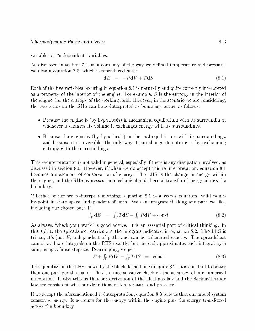
Thermodynamic Paths and Cycles 83

variables or independent variables.

As discussed in section 7.4, as a corollary of the way we dened temperature and pressure,we obtain equation 7.8, which is reproduced here:

dE = −PdV + TdS (8.1)

Each of the ve variables occuring in equation 8.1 is naturally and quite correctly interpretedas a property of the interior of the engine. For example, S is the entropy in the interior ofthe engine, i.e. the entropy of the working uid. However, in the scenario we are considering,the two terms on the RHS can be re-interpreted as boundary terms, as follows:

Because the engine is (by hypothesis) in mechanical equilibrium with its surroundings,whenever it changes its volume it exchanges energy with its surroundings.

Because the engine is (by hypothesis) in thermal equilibrium with its surroundings,and because it is reversible, the only way it can change its entropy is by exchangingentropy with the surroundings.

This re-interpretation is not valid in general, especially if there is any dissipation involved, asdiscussed in section 8.6. However, if/when we do accept this re-interpretation, equation 8.1becomes a statement of conservation of energy. The LHS is the change in energy withinthe engine, and the RHS expresses the mechanical and thermal transfer of energy across theboundary.

Whether or not we re-interpret anything, equation 8.1 is a vector equation, valid point-by-point in state space, independent of path. We can integrate it along any path we like,including our chosen path Γ.∫

ΓdE =

∫ΓTdS −

∫ΓPdV + const (8.2)

As always, check your work is good advice. It is an essential part of critical thinking. Inthis spirit, the spreadsheet carries out the integrals indicated in equation 8.2. The LHS istrivial; it's just E, independent of path, and can be calculated exactly. The spreadsheetcannot evaluate integrals on the RHS exactly, but instead approximates each integral by asum, using a nite stepsize. Rearranging, we get

E +∫

ΓPdV −

∫ΓTdS = const (8.3)

This quantity on the LHS shown by the black dashed line in gure 8.2. It is constant to betterthan one part per thousand. This is a nice sensitive check on the accuracy of our numericalintegration. It also tells us that our derivation of the ideal gas law and the Sackur-Tetrodelaw are consistent with our denitions of temperature and pressure.

If we accept the aforementioned re-interpretation, equation 8.3 tells us that our model systemconserves energy. It accounts for the energy within the engine plus the energy transferredacross the boundary.


8.1.2 Out-of-State Functions

Let's give names to the two integrals on the RHS of equation 8.2. We dene the work doneby the engine to be:

WΓ(θ) :=∫

ΓPdV (8.4)

where the integral runs over all θ′ on the path Γ, starting at θ′ = 0 and ending at θ′ = θ.We call WΓ the work done by the engine along the path Γ. This terminology is consistentwith ordinary, customary notions of work.

We also dene the heat absorbed by the engine to be:

QΓ(θ) :=∫

ΓTdS (8.5)

For present purposes, we call this the heat absorbed by the engine along the specied path.This is consistent with some commonly-encountered dentions of heat.1

Figure 8.3 includes all the curves from gure 8.2 plus heat (as shown by the brown curve)and work (as shown by the black curve).

Figure 8.3: State and Out-of-State Functions versus Arc Length

It should be clear in gure 8.3 that the black and brown curves are quite unlike the othercurves. Specically, they are not functions of state. They are functions of the arc length θalong the path γ, but they are not functions of the thermodynamic state X. Every timethe path returns to the point X0 in state space, WΓ(θ) takes on a dierent value, dierentfrom what it was on the previous cycle. Similarly QΓ(θ) takes on a dierent value. You cansee this in the gure, especially at places where θ takes on integer values. The state of theengine is the same at each of these places, but the heat and work are dierent.

1... but not all, especially if there is any dissipation involved.


Heat and work are plotted in gure 8.3, but there is no hope of plotting them on a (P, V )diagram such as gure 8.1.

Suppose we continue the operation of this heat engine for more cycles, keeping the cyclesalways in the vicinity of X0.

The state variables such as P , V , T , etcetera will remain bounded, returning totheir initial values every time the path Γcrosses the initial point X0.

The WΓ(θ) and QΓ(θ) curves will con-tinue marching o to the northeast, with-out bound.

At any point X in state space, if you knowX you know the associated values of thestate functions, and the state functionsdon't care how you got to X.

At any point X in state space, even if Xis somewhere on the path Γ, knowing Xis not sucient to determine out-of-statefunctions such as QΓ(θ), WΓ(θ), or θ itself.The out-of-state functions very much de-pend on how you got to X.

8.1.3 Converting Out-of-State Functions to State Functions

Suppose you start with TdS and you want to integrate it. There are at least three possibil-ities:

You can add something, namely −PdV , and then integrate. This gives you the energyE, which is a function of state. The value of the integral depends on the endpoints ofthe path, but not on other details of the path.

You can multiply by something , namely 1/T , and then integrate. This gives youthe entropy S, which is a function of state. The value of the integral depends on theendpoints of the path, but not on other details of the path.

You can integrate TdS along some chosen path, and accept the fact that the result isnot a function of state. The value of the integral depends on every detail of the chosenpath.

Please keep in mind that in modern thermodynamics, we dene entropy in terms of theprobability of the microstates, as discussed in connection with equation 2.2. However, backin pre-modern times, before 1898, people had no understanding of microstates. Quite re-markably, they were able to calculate the entropy anyway, in simple situations, using thefollowing recipe:

Build a reversible heat engine.


Measure QΓ(θ). That is, measure the heat absorbed by the engine as a function of arclength, as the engine goes through its cycles along the path Γ.

Dierentiate with respect to θ.

Multiply by 1/T .

Integrate with respect to θ.

The interesting thing is that even though this recipe depends explicitly on a particular pathΓ, the result is path-independent. The result gives you S as a function of state (plus orminus some constant of integration) independent of path.

Back in pre-modern times, people not only used this recipe to calculate the entropy, theyused it to dene entropy. It is not a very convenient denition. It is especially inconvenientin situations where dissipation must be taken into account. That's partly because it becomesless than obvious how to dene and/or measure QΓ.

8.1.4 Reversibility and/or Uniqueness

In our scenario, we choose to operate the heat engine such a way that it moves reversiblyalong the path Γ in gure 8.1. Every step along the path is done reversibly. There is no lawof physics that requires this, but we can make it so (to a good approximation) by suitableengineering.

We can also treat each of the ve cycles as a separate path. If we do that, it becomes clearthat there are innitely many paths going through the point X0. More generally, the samecan be said of any other point in state space: there are innitely many paths going throughthat point. As a corollary, given any two points on an indicator diagram, there are inntelymany paths from one to the other. Even if we restrict attention to reversible operations,there are still innitely many paths from one point to the other.

As a separate matter, we assert that any path through the state-space of the engine can befollowed reversibly (to a good approximation) or irreversibly. There is no way of looking ata diagram such as gure 8.1 and deciding whether a path is reversible or not. Reversibilitydepends on variables that are not shown in the diagram. Specically, when some step alongthe path is associated with a change in system entropy, the step is either reversible or not,depending on what happens outside the system. If there is an equal-and-opposite change inthe entropy of the surroundings, the step is reversible, and not otherwise.

I mention this because sometimes people who ought to know better speak of the reversiblepath between two points on a (P, V ) diagram. This is wrong at least twice over.


There is no such thing as a reversible path in a (P, V ) diagram. (You could imaginetalking about reversible paths if you constructed a higher-dimensional diagram, includ-ing the variable describing not just the heat engine but its surroundings as well, butthat's a dierent story. That would be a complicated and rather unusual diagram.)

Even if we restrict attention to reversible operations, there is no such thing as theunique path in uncramped thermodynamics. To say the same thing the other way, ifthe system is so cramped that there is only one path from one (P, V ) point to another,it is obviously impossible to build a heat engine.

8.1.5 The Importance of Out-of-State Functions

As we shall see, state functions are more elegant than out-of-state functions. They are vastlyeasier to work with. Usually, anything that can be expressed in terms of state functionsshould be.

However, out-of-state functions remain importance. The entire raison d'être of a heat engineis to convert heat into work, so it's nice to have a good way to quantify what we mean byheat and work.

An electric power company provides each customer with a watt-hour meter, which measuresthe electrical work done. The customer's bill largely depends on the amount of work done,so this is an example of an out-of-state function with tremendous economic signicance.

Also note that in pre-modern thermodynamics, heat was super-important, because it waspart of the recipe for dening entropy, as discussed in section 8.1.3.

8.1.6 Heat Content, or Not

In cramped thermodynamics, heat content is a state function. You can heat up a bottle ofmilk and let it cool down, in such a way that the energy depends on the temperature andthe heat capacity, and that's all there is to it.

However, in uncramped thermodynamics, there is no such thing as heat content. You candene QΓ as a function of arc length along a specied path, but it is not a state functionand it cannot be made into a state function.

More-or-less everybody who studies thermodynamics gets to the point where they try toinvent a heat-like quantity that is a function of state, but they never succeed. For more onthis, see section 8.2 and chapter 17.


8.1.7 Some Mathematical Remarks

If you ever have something that looks like heat and you want to dierentiate it, refer backto the denition in equation 8.5 and write the derivative as TdS. That is elegant, becauseas discussed in section 8.2 and elsewhere, T is a state function S is a state function, dS isa state function, and the product TdS is a state function. This stands in contrast to QΓ

which is not a state function, and dQ which does not even exist.

It is possible to dierentiate QΓ if you are very very careful. It is almost never worth thetrouble because you are better o with TdS but it can be done. As a corollary ofequation 8.1, equation 8.4, and equation 8.5, we can write:

ddθE(XΓ) = d

dθQΓ − ddθWΓ (8.6)

which is of course shorthand forddθE(XΓ(θ)) = d

dθQΓ(θ)− ddθWΓ(θ) (8.7)

Whereas equation 8.1 is a vector equation involving gradient vectors, equation 8.6 is a scalarequation involving total derivatives with respect to θ. It can be understood as a projectionof equation 8.1, obtained by projecting the gradient vectors onto the direction specied bythe path Γ.

On the LHS of equation 8.6, we might be able to consider the energy E to be a functionof state, especially if we we can write as E(X), which does not depend on the path Γ.However, if we write it as E(XΓ), the energy depends indirectly on the path. In particular,the derivative on the LHS of equation 8.6 very much depends on the path. Considered as aderivative in state space, it is a directional derivative, in the direction specied by the path.

Here is where non-experts go o the rails: In equation 8.6, it is tempting (but wrong) tosimplify the equation by dropping the dθ that appears in every term. Similarly it istempting (but wrong) to simplify the equation by dropping the Γ that appears in everyterm. The fact of the matter is that these are directional derivatives, and the directionmatters a great deal. If you leave out the direction-speciers, the derivatives simply do notexist.

8.2 Grady and Ungrady One-Forms

Sometimes people who are trying to write equation 8.6 instead write something like:

dE = dQ− dW (allegedly) (8.8)

which is deplorable.

Using the language of dierential forms, the situation can be understood as follows:• E is a scalar state-function.


• V is a scalar state-function.• S is a scalar state-function.• P is a scalar state-function.• T is a scalar state-function.• ∆E := E2 − E1 is a scalar function of two states.• ∆S := S2 − S1 is a scalar function of two states.• ∆V := V2 − V1 is a scalar function of two states.• dE is a grady one-form state-function.• dS is a grady one-form state-function.• dV is a grady one-form state-function.• w := PdV is in general an ungrady one-form state-function.• q := TdS is in general an ungrady one-form state-function.• There is in general no state-function W such that w = dW .• There is in general no state-function Q such that q = dQ.

where in the last four items, we have to say in general because exceptions can occur inpeculiar situations, mainly cramped situations where it is not possible to construct a heatengine. Such situations are very unlike the general case, and not worth much discussionbeyond what was said in conjunction with equation 7.37. When we say something is a state-function we mean it is a function of the thermodynamic state. The last two items followimmediately from the denition of grady versus ungrady.

Beware that in one dimension, ∆S is rather similar to dS. However, that's not true inhigher dimensions ... and uncramped thermodynamics is intrinsically multi-dimensional. Ifyou have experience in one dimension, do not let it mislead you. Recognize the fact that ∆Sis a scalar, whereas dS is a vector.

Figure 8.4 shows the dierence between a grady one-form and an ungrady one-form.

As you can see in on the left side of the g-ure, the quantity dS is grady. If you inte-grate clockwise around the loop as shown,the net number of upward steps is zero.This is related to the fact that we can as-sign an unambiguous height (S) to eachpoint in (T, S) space.

In contrast, as you can see on the right sideof the diagram, the quantity TdS is notgrady. If you integrate clockwise aroundthe loop as shown, there are considerablymore upward steps than downward steps.There is no hope of assigning a height Qto points in (T, S) space.

Some additional diagrams showing the relationship between certain grady and ungrady one-forms, see section 15.2.2. For details on the properties of one-forms in general, see reference 4and perhaps reference 23.

Be warned that in the mathematical literature, what we are callingungrady one-forms are called inexact one-forms. The two terms areentirely synonymous. A one-form is called exact if and only if it


Figure 8.4: dS is Grady, TdS is Not

is the gradient of something. We avoid the terms exact and inex-act because they are too easily misunderstood. In particular, in thiscontext,• exact is not even remotely the same as accurate.• inexact is not even remotely the same as inaccurate.• inexact does not mean plus or minus something.• exact just means grady. An exact one-form is the gradient of somepotential.

The dierence between grady and ungrady has important consequences for practical situ-ations such as heat engines. Even if we restrict attention to reversible situations, we stillcannot think of Q as a function of state, for the following reasons: You can dene any num-ber of functions Q1, Q2, · · · by integrating TdS along some paths Γ1,Γ2, · · · of your choosing.Each such Qi can be interpreted as the total heat that has owed into the system along the

specied path. As an example, let's choose Γ6 to be the path that a heat engine follows asit goes around a complete cycle a reversible cycle, perhaps something like a Carnot cycle,as discussed in section 8.7. Let Q6(N) be the value of Q6 at the end of the Nth cycle. Wesee that even after specifying the path, Q6 is still not a state function, because at the end ofeach cycle, all the state functions return to their initial values, whereas Q6(N) grows linearlywith N . This proves that in any situation where you can build a heat engine, q is not equal


to d(anything).

8.3 Abuse of the Notation

Suppose there are two people, namely wayne and dwayne. There is no special relationshipbetween them. In particular, we interpret dwayne as a simple six-letter name, not asd(wayne) i.e. not as the derivative of wayne.

Some people try to use the same approach to supposedly dene dQ to be a two-letter namethat represents T dS supposedly without implying that dQ is the derivative of anything.That is emphatically not acceptable. That would be a terrible abuse of the notation.

In accordance with almost-universally accepted convention, d is an operator, and dQ denotesthe operator d applied to the variable Q. If you give it any other interpretation, you aregoing to confuse yourself and everybody else.

The point remains that in thermodynamics, there does not exist any Q such that dQ = T dS(except perhaps in trivial cases). Wishing for such a Q does not make it so. See chapter 19for more on this.

8.4 Procedure for Extirpating dW and dQ

Constructive suggestion: If you are reading a book that uses dW and dQ, you can repair itusing the following simple procedure:

For reversible processes, it's easy: Every time you see dQ, cross it out and write T dSinstead. Every time you see dW , cross it out and write P dV or −P dV instead. Thechoice of sign depends on convention. It should be easy to determine which conventionthe book is using.

For irreversible processes, much more eort is required. Classical thermodynamicsbooks like to say that for an irreversible process T dS is greater than dQ. In thiscase, you can't simply replace dQ by T dS because dQ (to the extent that it meansanything at all) sometimes does not account for the entire T dS. In this context,it probably involves only the entropy that owed in across the boundary not theentropy that was created from scratch. So the rule in this context is to cross out dQand replace it by T dStransferred.

As for the idea that T dS > T dStransferred for an irreversible process, we cannotaccept that at face value. For one thing, we would have problems at negative temper-atures. We can x that by getting rid of the T on both sides of the equation. Another


problem is that according to the modern interpretation of the symbols, dS is a vector,and it is not possible to dene a greater-than relation involving vectors. That is tosay, vectors are not well ordered. We can x this by integrating. The relevant equationis: ∫

ΓdS =

∫Γ(dStransferred + dScreated)

>∫

ΓdStransferred

(8.9)

for some denite path Γ. We need Γ to specify the forward direction of the transfor-mation; otherwise the inequality wouldn't mean anything. We have an inequality, notan equality, because we are considering an irreversible process.

At the end of the day, we nd that the assertion that T dS is greater than dQ is justa complicated and defective way of saying that the irreversible process created someentropy from scratch.

Note: The underlying idea is that for an irreversible process, entropy is not conserved,so we don't have continuity of ow. Therefore the classical approach was a bad idea tobegin with, because it tried to dene entropy in terms of heat divided by temperature,and tried to dene heat in terms of ow. That was a bad idea on practical grounds andpedagogical grounds, in the case where entropy is being created from scratch ratherthan owing. It was a bad idea on conceptual grounds, even before it was expressedusing symbols such as dQ that don't make sense on mathematical grounds.

Beware: The classical thermo books are inconsistent. Even within a single book, evenwithin a single chapter, sometimes they use dQ to mean the entire T dS and sometimesonly the T dStransferred.

8.5 Some Reasons Why dW and dQ Might Be Tempting

It is remarkable that people are fond of writing things like dQ . . . even in cases where it doesnot exist. (The remarks in this section apply equally well to dW and similar monstrosities.)

Even people who know it is wrong do it anyway. They call dQ an inexact dierential andsometimes put a slash through the d to call attention to this. The problem is, neither dQnor Q is a dierential at all. Yes, TdS is an ungrady one-form or (equivalently) an inexactone-form, but no, it is not properly called an inexact dierential, since it is generally not adierential at all. It is not the derivative of anything.

One wonders how such a bizarre tangle of contradictions could arise, and how it could persist.I hypothesize part of the problem is a too-narrow interpretation of the traditional notationfor integrals. Most mathematics books say that every integral should be written in the form∫

(integrand)d(something) (8.10)


where the d is alleged to be merely part of the notation an obligatory and purely mechanicalpart of the notation and the integrand is considered to be separate from the d(something).

However, it doesn't have to be that way. If you think about a simple scalar integral from theLebesgue point of view (as opposed to the Riemann point of view), you realize that what isindispensable is a weighting function. Specically: d(something) is a perfectly ne, normaltype of weighting function, but not the only possible type of weighting function.

In an ordinary one-dimensional integral, we are integrating along a path, which in the sim-plest case is just an interval on the number line. Each element of the path is a little pointyvector, and the weighing function needs to map that pointy vector to a number. Any one-form will do, grady or otherwise. The grady one-forms can be written as d(something), whilethe ungrady ones cannot.

For purposes of discussion, in the rest of this section we will put square brackets around theweighting function, to make it easy to recognize even if it takes a somewhat unfamiliar form.As a simple example, a typical integral can be written as:∫

Γ

(integrand)[(weight)] (8.11)

where Γ is the domain to be integrated over, and the weight is typically something like dx.

As a more intricate example, in two dimensions the moment of inertia of an object Ω is:

I :=

∫Ω

r2[dm] (8.12)

where the weight is dm. As usual, r denotes distance and m denotes mass. The integralruns over all elements of the object, and we can think of dm as an operator that tells usthe mass of each such element. To my way of thinking, this is the denition of moment ofinertia: a sum of r2, summed over all elements of mass in the object.

The previous expression can be expanded as:

I =

∫Ω

r2[ρ(x, y)dxdy] (8.13)

where the weighting function is same as before, just rewritten in terms of the density, ρ.

Things begin to get interesting if we rewrite that as:

I =

∫Ω

r2ρ(x, y)[dxdy] (8.14)

where ρ is no longer part of the weight but has become part of the integrand. We see thatthe distinction between the integrand and the weight is becoming a bit vague. Exploitingthis vagueness in the other direction, we can write:

I =∫

Ω[r2 dm]

=∫

Ω[r2 ρ(x, y)dxdy]

(8.15)


which tells us that the distinction between integrand and weighting function is completelymeaningless. Henceforth I will treat everything inside the integral on the same footing. Theintegrand and weight together will be called the argument2 of the integral.

Using an example from thermodynamics, we can writeQΓ =

∫ΓT [dS]

=∫

Γ[T dS]

=∫

Γ[q]

(8.16)

where Γ is some path through thermodynamic state-space, and where q is an ungrady one-form, dened as q := TdS.

It must be emphasized that these integrals must not be written as∫

[dQ] nor as∫

[dq]. Thisis because the argument in equation 8.16 is an ungrady one-form, and therefore cannot beequal to d(anything).

There is no problem with using TdS as the weighting function in an integral. The onlyproblem comes when you try to write TdS as d(something) or (something):• Yes, TdS is a weighting function.• Yes, it is a one-form.• No, it is not a grady one-form.• No, it is not d(anything).

I realize an expression like∫

[q] will come as a shock to some people, but I think it expressesthe correct ideas. It's a whole lot more expressive and more correct than trying to writeTdS as d(something) or (something).

Once you understand the ideas, the square brackets used in this section no longer serve anyimportant purpose. Feel free to omit them if you wish.

There is a proverb that says if the only tool you have is a hammer, everything begins to looklike a nail. The point is that even though a hammer is the ideal tool for pounding nails, it issuboptimal for many other purposes. Analogously, the traditional notation

∫· · ·dx is ideal

for some purposes, but not for all. Specically: sometimes it is OK to have no explicit dinside the integral.

There are only two things that are required: the integral must have a domain to be integratedover, and it must have some sort of argument. The argument must be an operator, whichoperates on an element of the domain to produce something (usually a number or a vector)that can be summed by the integral.

A one-form certainly suces to serve as an argument (when elements of the domain arepointy vectors). Indeed, some math books introduce the notion of one-forms by dening

2This corresponds to saying that θ is the argument of the cosine in the expression cos(θ).


them to be operators of the sort we need. That is, the space of one-forms is dened as anoperator space, consisting of the operators that map column vectors to scalars. (So onceagain we see that one-forms correspond to row vectors, assuming pointy vectors correspondto column vectors). Using these operators does not require taking a dot product. (Youdon't need a dot product unless you want to multiply two column vectors.) The operationof applying a row vector to a column vector to produce a scalar is called a contraction, nota dot product.

It is interesting to note that an ordinary summation of the form∑

i Fi corresponds exactlyto a Lebesgue integral using a measure that assigns unit weight to each integer (i) in thedomain. No explicit d is needed when doing this integral. The idea of weighting functionis closely analogous to the idea of measure in Lebesgue integrals, but not exactly thesame. We must resist the temptation to use the two terms interchangeably. In particular, ameasure is by denition a scalar, but sometimes (such as when integrating along a curve) itis important to use a weighting function that is a vector.

People heretofore have interpreted d inseveral ways: as a dierential operator(with the power, among other things, toproduce one-forms from scalars), as an in-nitesimal step in some direction, and asthe marker for the weighting function inan integral. The more I think about it, themore convinced I am that the dierentialoperator interpretation is far and away themost advantageous. The other interpreta-tions of d can be seen as mere approxima-tions of the operator interpretation. Theapproximations work OK in elementarysituations, but produce profound miscon-ceptions and contradictions when appliedto more general situations . . . such as ther-modynamics.

In contrast, note that in section 17.1, I donot take such a hard line about the mul-tiple incompatible denitions of heat. Idon't label any of them as right or wrong.Rather, I recognize that each of them in

isolation has some merit, and it is onlywhen you put them together that conictsarise.

Bottom line: There are two really simple ideas here: (1) d always means exterior derivative.The exterior derivative of any scalar-valued function is a vector. It is a one-form, not apointy vector. In particular it is always a grady one-form. (2) An integral needs to have aweighting function, which is not necessarily of the form d(something).

8.6 Boundary versus Interior

We now discuss two related notions:• The ow of something across the boundary of the region.


• The change in the amount of something inside the region.

When we consider a conserved quantity such as energy, momentum, or charge, these twonotions stand in a one-to-one relationship. In general, though, these two notions are notequivalent.

In particular, consider equation 7.39, which is restated here:

dE = −PdV + TdS + advection (8.17)

Although ocially dE represents the change in energy in the interior of the region, we arefree to interpret it as the ow of energy across the boundary. This works because E is aconserved quantity.

The advection term is explicitly a boundary-ow term.

It is extremely tempting to interpret the two remaining terms as boundary-ow terms also. . . but this is not correct!

Ocially PdV describes a property of the interior of the region. Ditto for TdS. Neitherof these can be converted to a boundary-ow notion, because neither of them represents aconserved quantity. In particular, PdV energy can turn into TdS energy entirely within theinterior of the region, without any boundary being involved.

Let's be clear: boundary-ow ideas are elegant, powerful, and widely useful. Please don'tthink I am saying anything bad about boundary-ow ideas. I am just saying that the PdVand TdS terms do not represent ows across a boundary.

Misinterpreting TdS as a boundary term is a ghastly mistake. It is more-or-less tantamountto assuming that heat is a conserved quantity unto itself. It would set science back over 200years, back to the caloric theory.

Once these mistakes have been pointed out, they seem obvious, easy to spot, and easyto avoid. But beware: mistakes of this type are extremely prevalent in introductory-levelthermodynamics books.

8.7 The Carnot Cycle

A Carnot cycle is not the only possible thermodynamic cycle, or even the only reversiblecycle, but it does have special historical and pedagogical signicance. Because it is easy toanalyze, it gets more attention than it really deserves, which falls into the catetory of lookingunder the lamp-post. The Carnot cycle involves only relatively simple operations, namelyisothermal expansion and contraction and thermally isolated expansion and contraction. It isfairly easy to imagine carrying out such operations without introducing too much dissipation.


The topic of Carnot cycle is only tangentially related to the topic of Carnoteciency. The topics are related insofar as the eciency of the Carnot cycle isparticularly easy to calculate. However, the denition of eciency applies to afar broader class of cycles, as discussed in section 6.5.

In this section, we do a preliminary analysis of the Carnot cycle. We carry out the analysisusing two slightly dierent viewpoints, running both analyses in parallel. In gure 8.5 andgure 8.6 the physics is the same; only the presentation is dierent. The primary dierence isthe choice of axes: (V, T ) versus (P, T ). Every other dierence can be seen as a consequenceof this choice.

In gure 8.5: In gure 8.6:

When the engine is doing work we go clock-wise around the cycle.

When the engine is doing work we go coun-terclockwise around the cycle.

In other words, the sequence for positive work being done by the engine is this: red, black,magenta, blue.

0 1 2 3 4 5 6

Volume

0.0

0.2

0.4

0.6

0.8

1.0

Temperature

0 1 2 3 4

Pressure

0.0

0.2

0.4

0.6

0.8

1.0

Temperature

Figure 8.5: Carnot Cycle : T versus VFigure 8.6: Carnot Cycle : T versus P

In all of these gures, the contours of constant pressure are shown in white. The pressurevalues form a geometric sequence: 1/8, 1/4, 1/2, 1, 2. In gure 8.6 this is obvious, butin the other gures you will just have to remember it. The P = 1/8 contour is shown as adotted line, to make it easy to recognize. The P = 1 contour goes through the corner wherered meets black.

There are at least a dozen dierent ways of plotting this sort of data. Another version isshown in gure 8.7. It is somewhat remarkable that multiple gures portraying the samephysics would look so dierent at rst glance. I diagrammed the situation in multipleways partly to show the dierence, and partly to make again the point that any of thethermodynamic state-functions can be drawn as a function of any reasonable set of variables.

The spreadsheet used to compute these diagrams is cited in reference 24.


0 1 2 3 4 5 6

Volume

0.0

0.5

1.0

1.5

2.0

2.5

Entropy

Figure 8.7: Carnot Cycle : S versus V

It's interesting that we can replot the data in such a way as to change the apparent shape ofthe diagram ... without changing the meaning. This claries something that was mentionedin goal 5 in section 0.3: In thermodynamic state-space, there is a topology but not a geometry.We can measure the distance (in units of S) between contours of constant S, but we cannotcompare that to any distance in any other direction.

In thermodynamics, there are often more variables than one can easily keep track of. Herewe focus attention on T , V , P , and S. There are plenty of other variables (such as E) thatwe will barely even mention. Note that the number of variables far exceeds the number ofdimensions. We say this is a two-dimensional situation, because it can be projected onto atwo-dimensional diagram without losing any information.

It takes some practice to get the hang of interpreting these diagrams.

In gure 8.5:

Contours of constant temperature are horizontal lines. Examples include the redand magenta path-segments.

Contours of constant volume are vertical lines. These are not explicitly shown,but you can easily gure out what they would look like.

Contours of constant pressure are sloping lines, shown in white.

Contours of constant entropy are curves. Examples include the blue and blackpath-segments.

In gure 8.6:

Contours of constant temperature are horizontal lines. Examples include the redand magenta path-segments.

Contours of constant volume are not shown. (They would be sloping lines, forminga starburst pattern similar to the white lines in gure 8.5.)

Contours of constant pressure are vertical lines, shown in white.


Contours of constant entropy are curves. Examples include the blue and blackpath-segments.

In gure 8.7:

Contours of constant temperature are curves. Examples include the red andmagenta path-segments.

Contours of constant volume are vertical lines. These are not explicitly shown,but you can easily gure out what they would look like.

Contours of constant pressure are curves, shown in white.

Contours of constant entropy are horizontal lines. Examples include the blue andblack path-segments.

The Carnot cycle has four phases.

1. Isothermal expansion: We connect the cylinder to the high-temperature heat bath.We gently expand the gas at constant high temperature. This is shown in red in thegures.

The amount of expansion is a design choice. In the example I arbitrarily chose avolume ratio of 3.5:1 for this phase of the expansion. (This is not the so-called com-pression ratio of the overall engine, since we have so far considered only one of thetwo compression phases.)

2. Isentropic expansion: We disconnect the cylinder. We expand the gas some more,gently, at constant entropy. This is shown in black in the gures.

We continue the expansion until the temperature of the gas reaches the temperatureof the low-temperature heat bath.

The amount of expansion required to achieve this depends on the gamma of the gas and(obviously) on the ratio of temperatures. For the example I assumed a 2:1 temperatureratio, which calls for a 5.7:1 expansion ratio during this phase. In general, for anadiabatic expansion, if you know the temperature ratio you can calculate the expansionratio for this phase via

V1V2

=(T1T2

)−1/(γ−1)(8.18)

For the gures I used the gamma value appropriate for air and similar diatomic gases,namely γ = 7/5 = 1.4. A monatomic gas would need a signicantly lower compressionratio for any given temperature ratio.

3. Isothermal compression: We connect the cylinder to the low-temperature heat bath.We gently compress the gas at constant low temperature. This is shown in magentain the gures.


4. Isentropic compression: We disconnect the cylinder from both heat baths. We compressthe gas some more, gently, along a contour of constant entropy. This is shown in bluein the gures.

During the two expansion phases, the gas does work on the ywheel. During the two com-pression phases, the ywheel needs to do work on the gas. However, the compression-workis strictly less in magnitude than the expansion-work, so during the cycle net energy isdeposited in the ywheel.

To understand this at the next level of detail, recall that mechanical work is −P dV . Nowthe integral of dV around the cycle is just ∆V which is zero. But what about the integralof P dV ? Consider for example the step in V that goes from V = 3 to V = 4 along theblack curve, and the corresponding step that goes from V = 4 to V = 3 along the magentacurve. The work done during the expansion phase (black) will be strictly greater than thework done during the recompression phase (magenta) because the pressure is higher. Youcan make the same argument for every piece of V in the whole V -space: For every ∆V inone of the expansion phases there will be a corresponding ∆V directly below it in one of thecompression phases. For each of these pairs, expansion-work will be strictly greater than thecompression-work because the pressure will be higher.

You can infer the higher pressure from the white contours of constant pressure, or you canjust observe that the pressure must be higher because the temperature is higher.

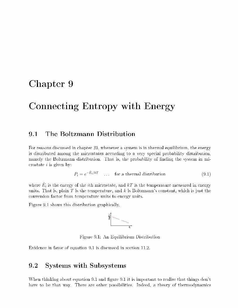
Chapter 9

Connecting Entropy with Energy

9.1 The Boltzmann Distribution

For reasons discussed in chapter 23, whenever a system is in thermal equilibrium, the energyis distributed among the microstates according to a very special probability distribution,namely the Boltzmann distribution. That is, the probability of nding the system in mi-crostate i is given by:

Pi = e−Ei/kT . . . for a thermal distribution (9.1)

where Ei is the energy of the ith microstate, and kT is the temperature measured in energyunits. That is, plain T is the temperature, and k is Boltzmann's constant, which is just theconversion factor from temperature units to energy units.

Figure 9.1 shows this distribution graphically.

Ei

ilo

g(

)

P

Figure 9.1: An Equilibrium Distribution

Evidence in favor of equation 9.1 is discussed in section 11.2.

9.2 Systems with Subsystems

When thinking about equation 9.1 and gure 9.1 it is important to realize that things don'thave to be that way. There are other possibilities. Indeed, a theory of thermodynamics


that assumed that everything in sight was always in equilibrium at temperature T would benot worth the trouble. For starters, it is impossible to build a heat engine unless the hotreservoir is not in equilibrium with the cold reservoir.

We start by considering the system shown in gure 9.2, namely a styrofoam box containinga hot potato and a cold potato. (This is a simplied version of gure 1.2.)

Hot Potato Cold Potato

Figure 9.2: A System Consisting of Two Potatoes

In situations like this, we can make good progress if we divide the system into subsystems.Here subsystem A is the red potato, and subsystem B is the blue potato. Each subsystemhas a well dened temperature, but initially the system as a whole does not.

If we wait long enough, the two potatoes will come into equilibrium with each other, and atthis point the system as a whole will have a well dened temperature. However, we are notrequired to wait for this to happen.

Connecting Entropy with Energy 93

0 50 100 150 200 250

Subsystem Microstate Energy

−3

−2

−1

0

log P

robabili

ty

red potatoblue potato

Figure 9.3: Probability versus Energy, Non-Equilibrium

0 50 100 150 200 250

System Microstate Energy

−3

−2

−1

0

log P

rob

abili

ty

before equilibrationafter equilibration

Figure 9.4: Probability versus Energy, System as a Whole


9.3 Remarks

9.3.1 Predictable Energy is Freely Convertible

The dierence between random energy and predictable energy has many consequences. Themost important consequence is that the predictable energy can be freely converted to andfrom other forms, such as gravitational potential energy, chemical energy, electrical energy,et cetera. In many cases, these conversions can be carried out with very high eciency.In some other cases, though, the laws of thermodynamics place severe restrictions on theeciency with which conversions can be carried out, depending on to what extent the energydistribution deviates from the Boltzmann distribution.

9.3.2 Thermodynamic Laws without Temperature

Ironically, the rst law of thermodynamics (equation 1.1) does not depend on temperature.Energy is well-dened and is conserved, no matter what. It doesn't matter whether thesystem is hot or cold or whether it even has a temperature at all.

Even more ironically, the second law of thermodynamics (equation 2.1) doesn't depend ontemperature, either. Entropy is well-dened and is paraconserved no matter what. It doesn'tmatter whether the system is hot or cold or whether it even has a temperature at all.

(This state of aairs is ironic because thermodynamics is commonly dened to be the scienceof heat and temperature, as you might have expected from the name: thermodynamics. Yetin our modernized and rationalized thermodynamics, the two most central, fundamentalideas energy and entropy are dened without reference to heat or temperature.)

Of course there are many important situations that do involve temperature. Most of thecommon, every-day applications of thermodynamics involve temperature but you shouldnot think of temperature as the essence of thermodynamics. Rather, it is a secondary conceptwhich is dened (if and when it even exists) in terms of energy and entropy.

9.3.3 Kinetic and Potential Microscopic Energy

You may have heard the term kinetic theory. In particular, the thermodynamics of idealgases is commonly called the kinetic theory of gases. However, you should be careful, becausekinetic theory is restricted to ideal gases (indeed to a subset of ideal gases) ... whilethermodynamics applies to innumerable other things. Don't fall into the trap of thinking thatthere is such a thing as thermal energy and that this so-called thermal energy is necessarilykinetic energy. In almost all systems, including solids, liquids, non-ideal gases, and even someideal gases, the energy is a mixture of kinetic and potential energy. (Furthermore, in any


non-cramped situation, i.e. in any situation where it is possible to build a heat engine, it isimpossible in principle to dene any such thing as thermal energy.) In any case, it is saferand in all ways better to say thermodynamics or statistical mechanics instead of kinetictheory.

In typical systems, potential energy and kinetic energy play parallel roles:• To visualize microscopic potential energy, imagine that the atoms in a crystal latticeare held in place by springs. Roughly speaking, half of these springs have positivepotential energy because they are extended relative to their resting-length, while theother half have positive potential energy because they are compressed relative to theirresting-length. They've all got energy, but you can't easily harness it because youdon't know which ones are compressed and which ones are extended.• To visualize microscopic kinetic energy, imagine that half the atoms have a leftwardvelocity and half have a rightward velocity. They all have kinetic energy, but you can'teasily harness it because you don't know which ones are moving leftward and whichare moving rightward.

In fact, for an ordinary crystal such as quartz or sodium chloride, almost exactly half of theheat capacity is due to potential energy, and half to kinetic energy. It's easy to see why thatmust be: The heat capacity is well described in terms of thermal phonons in the crystal. Eachphonon mode is a harmonic1 oscillator. In each cycle of any harmonic oscillator, the energychanges from kinetic to potential and back again. The kinetic energy goes like sin2(phase)and the potential energy goes like cos2(phase), so on average each of those is half of the totalenergy.

Not all kinetic energy contributes to the heat capacity.Not all of the heat capacitly comes from kinetic energy.

A table-top sample of ideal gas is a special case, where all the energy is kinetic energy. Thisis very atypical of thermodynamics in general. Table-top ideal gases are very commonlyused as an illustration of thermodynamic ideas, which becomes a problem when the exampleis overused so heavily as to create the misimpression that thermodynamics deals only withkinetic energy.

You could argue that in many familiar systems, the temperature is closely related to randomkinetic energy ... but temperature is not the same thing as so-called heat' or thermalenergy. Furthermore, there are other systems, such as spin systems, where the temperatureis not related to the random kinetic energy.

All in all, it seems quite unwise to dene heat or even temperature in terms of kinetic energy.

This discussion continues in section 9.3.4.

1Anharmonicity can cause the average KE to be not exactly equal to the average PE, but for a crystalwell below its melting point, the thermal phonon modes are not signicantly anharmonic.


9.3.4 Ideal Gas : Potential Energy as well as Kinetic Energy

We have seen that for an ideal gas, there is a one-to-one correspondence between the tem-perature and the kinetic energy of the gas particles. However, that does not mean that thereis a one-to-one correspondence between kinetic energy and heat energy. (In this context,heat energy refers to whatever is measured by a heat capacity experiment.)

To illustrate this point, let's consider a sample of pure monatomic nonrelativistic nondegen-erate ideal gas in a tall cylinder of horizontal radius r and vertical height h at temperatureT . The pressure measured at the bottom of the cylinder is P . Each particle in the gas hasmass m. We wish to know the heat capacity per particle at constant volume, i.e. CV /N .

At this point you may already have in mind an answer, a simple answer, a well-known answer,independent of r, h, m, P , T , and N . But wait, there's more to the story: The point of thisexercise is that h is not small. In particular, m|g|h is not small compared to kT , where gis the acceleration of gravity. For simplicity, you are encouraged to start by considering thelimit where h goes to innity, in which case the exact value of h no longer matters. Gravityholds virtually all the gas near the bottom of the cylinder, whenever h kT/m|g|.

Later, if you want to come back and work the problem a second time, with no restric-tions on h, that's interesting and not very dicult.

Also if you want to generalize to a polyatomic gas, that's also worth doing. Section 26.4continues the discussion of the energy of an ideal gas, including equation 26.46 andequation 26.47 which related energy to pressure, volume, and temperature.

You will discover that a distinctly nontrivial contribution to the heat capacity comes fromthe potential energy of the ideal gas. When you heat it up, the gas column expands, lifting itscenter of mass, doing work against gravity. (Of course, as always, there will be a contributionfrom the kinetic energy.)

For particles the size of atoms, the length-scale kT/m|g| is on the order of several kilometers,so the cylinder we are considering is much too big to t on a table top. I often use therestrictive term table-top as a shorthand way of asserting that m|g|h is small compared tokT .

So, this reinforces the points made in section 9.3.3. We conclude that in general, heat energyis not just kinetic energy.

Beware that this tall cylinder is not a good model for the earth's atmosphere.For one thing, the atmosphere is not isothermal. For another thing, if you aregoing to take the limit as h goes to innity, you can't use a cylinder; you needsomething more like a cone, spreading out as it goes up, to account for thespherical geometry.


9.3.5 Relative Motion versus Thermal Energy

Over the years, lots of people have noticed that you can always split the kinetic energy of acomplex object into the KE of the center-of-mass motion plus the KE of the relative motion(i.e. the motion of the components relative to the center of mass).

Also a lot of people have tried (with mixed success) to split the energy of an object into athermal piece and a non-thermal piece.

It is an all-too-common mistake to think that the overall/relative split is the same as thenonthermal/thermal split. Beware: they're not the same. Denitely not. See section 7.7 formore on this.

First of all, the microscopic energy is not restricted to being kinetic energy, as discussedin section 9.3.3. So trying to understand the thermal/non-thermal split in terms of kineticenergy is guaranteed to fail. Using the work/KE theorem (reference 18) to connect work(via KE) to the thermal/nonthermal split is guaranteed to fail for the same reason.

Secondly, a standard counterexample uses ywheels, as discussed in section 18.4. You canimpart macroscopic, non-Locrian KE to the ywheels without imparting center-of-mass KEor any kind of potential energy . . . and without imparting any kind of Locrian energy (eitherkinetic or potential).

The whole idea of thermal energy is problematic, and in many cases impossible to dene, asdiscussed in chapter 19. If you nd yourself worrying about the exact denition of thermalenergy, it means you're trying to solve the wrong problem. Find a way to reformulate theproblem in terms of energy and entropy.

Center-of-mass motion is an example but not the only example of low-entropy energy. Themotion of the ywheels is one perfectly good example of low-entropy energy. Several otherexamples are listed in section 11.3.

A macroscopic object has something like 1023 modes. The center-of-mass motion is just oneof these modes. The motion of counter-rotating ywheels is another mode. These are slightlyspecial, but not very special. A mode to which we can apply a conservation law, such asconservation of momentum, or conservation of angular momentum, might require a little bitof special treatment, but usually not much . . . and there aren't very many such modes.

Sometimes on account of conservation laws, and sometimes for other reasons as discussedin section 11.11 it may be possible for a few modes of the system to be strongly coupled tothe outside (and weakly coupled to the rest of the system), while the remaining 1023 modesare more strongly coupled to each other than they are to the outside. It is these issues ofcoupling-strength that determine which modes are in equilibrium and which (if any) are farfrom equilibrium. This is consistent with our denition of equilibrium (section 10.1).

Thermodynamics treats all the equilibrated modes on an equal footing. One manifestationof this can be seen in equation 9.1, where each state contributes one term to the sum . . . andaddition is commutative.


There will never be an axiom that says such-and-such mode is always in equilibrium oralways not; the answer is sensitive to how you engineer the couplings.

9.4 Entropy Without Constant Re-Shuing

It is a common mistake to visualize entropy as a highly dynamic process, whereby thesystem is constantly ipping from one microstate to another. This may be a consequence ofthe fallacy discussed in section 9.3.5 (mistaking the thermal/nonthermal distinction for thekinetic/potential distinction) . . . or it may have other roots; I'm not sure.

In any case, the fact is that re-shuing is not an essential part of the entropy picture.

An understanding of this point proceeds directly from fundamental notions of probabilityand statistics.

By way of illustration, consider one hand in a game of draw poker.

A) The deck is shued and hands are dealt in the usual way.

B) In preparation for the rst round of betting, you look at your hand and discover thatyou've got the infamous inside straight. Other players raise the stakes, and when it'syour turn to bet you drop out, saying to yourself if this had been an outside straightthe probability would have been twice as favorable.

C) The other players, curiously enough, stand pat, and after the hand is over you geta chance to ip through the deck and see the card you would have drawn.

Let's more closely examine step (B). At this point you have to make a decision based onprobability. The deck, as it sits there, is not constantly re-arranging itself, yet you aresomehow able to think about the probability that the card you draw will complete yourinside straight.

The deck, as it sits there during step (B), is not ipping from one microstate to another. Itis in some microstate, and staying in that microstate. At this stage you don't know whatmicrostate that happens to be. Later, at step (C), long after the hand is over, you might geta chance to nd out the exact microstate, but right now at step (B) you are forced to makea decision based only on the probability.

The same ideas apply to the entropy of a roomful of air, or any other thermodynamic system.At any given instant, the air is in some microstate with 100% probability; you just don'tknow what microstate that happens to be. If you did know, the entropy would be zero . . .but you don't know. You don't need to take any sort of time-average to realize that youdon't know the microstate.


The bottom line is that the essence of entropy is the same as the essence of probability ingeneral: The essential idea is that you don't know the microstate. Constant re-arrangementis not essential.

This leaves us with the question of whether re-arrangement is ever important. Of course thedeck needs to be shued at step (A). Not constantly re-shued, just shued the once.

Again, the same ideas apply to the entropy of a roomful of air. If you did somehow obtainknowledge of the microstate, you might be interested in the timescale over which the sys-tem re-arranges itself, making your erstwhile knowledge obsolete and thereby returning thesystem to a high-entropy condition.

The crucial point remains: the process whereby knowledge is lost and entropy is createdis not part of the denition of entropy, and need not be considered when you evaluate theentropy. If you walk into a room for the rst time, the re-arrangement rate is not yourconcern. You don't know the microstate of this room, and that's all there is to the story.You don't care how quickly (if at all) one unknown microstate turns into another.

If you don't like the poker analogy, we can use a cryptology analogy instead. Yes, physics,poker, and cryptology are all the same when it comes to this. Statistics is statistics.

If I've intercepted just one cryptotext from the opposition and I'm trying to crack it, on somelevel what matters is whether or not I know their session key. It doesn't matter whetherthat session key is 10 microseconds old, or 10 minutes old, or 10 days old. If I don't haveany information about it, I don't have any information about it, and that's all that need besaid.

On the other hand, if I've intercepted a stream of messages and extracted partial informationfrom them (via a partial break of the cryptosystem), the opposition would be well advised tore-shue the deck i.e. choose new session keys on a timescale fast compared to my abilityto extract information about them.

Applying these ideas to a roomful of air: Typical sorts of measurements give us only apathetically small amount of partial information about the microstate. So it really doesn'tmatter whether the air re-arranges itself super-frequently or super-infrequently. We don'thave any signicant amount of information about the microstate, and that's all there is tothe story.

Reference 25 presents a simulation that demonstrates the points discussed in this subsection.


9.5 Units of Entropy

Before we go any farther, convince yourself that

log10(x) =ln(x)

ln(10)

≈ 0.434294 ln(x)

(9.2)

and in general, multiplying a logarithm by some positive number corresponds to changingthe base of the logarithm.

In the formula for entropy, equation 2.2, the base of the logarithm has intentionally been leftunspecied. You get to choose a convenient base. This is the same thing as choosing whatunits will be used for measuring the entropy.

Some people prefer to express the units by choosing the base of the logarithm, while oth-ers prefer to stick with natural logarithms and express the units more directly, using anexpression of the form:

S[P ] := k∑i

Pi ln(1/Pi) (9.3)

In this expression we stipulated e as the base of the logarithm. Whereas equation 2.2 wecould choose the base of the logarithm, in equation 9.3 we get to choose the numerical valueand units for k. This is a supercially dierent solution to the same problem. Reasonablechoices include:

k = 1.3806504(24)×10−23 J/K= 1/ ln(3) trit= 1 nat= 1/ ln(2) bit

(9.4)

It must be emphasized that all these expressions are mathematically equivalent. In each case,the numerical part of k balances the units of k, so that the meaning remains unchanged. Insome cases it is convenient to absorb the numerical part of k into the base of the logarithm:

S[P ] = k∑

i Pi ln(1/Pi) (in general)= 1.3806504(24)×10−23

∑i Pi ln(1/Pi) J/K (SI)

=∑

i Pi logΩ(1/Pi) J/K (SI)=

∑i Pi log3(1/Pi) trit

=∑

i Pi loge(1/Pi) nat=

∑i Pi log2(1/Pi) bit

(9.5)

where the third line uses the remarkably huge base Ω = exp(1.24×1022). When dealingwith smallish amounts of entropy, units of bits are conventional and often convenient. When


dealing with large amounts of entropy, units of J/K are conventional and often convenient.These are related as follows:

1J/K = 1.04×1023bits1bit = 9.57×10−24J/K

(9.6)

A convenient unit for molar entropy is Joules per Kelvin per mole:1J/K/mol = 0.17bit/particle1bit/particle = 5.76J/K/mol = R ln(2)

(9.7)

Values in this range (on the order of one bit per particle) are very commonly encountered.

If you are wondering whether equation 9.7 is OK from a dimensional-analysispoint of view, fear not. Temperature units are closely related to energy units.Specically, energy is extensive and measured in J, while temperature is intensiveand measured in K. Therefore combinations such as (J/K/mol) are dimensionlessunits. A glance at the dimensions of the ideal gas law should suce to remindyou of this if you ever forget.

See reference 26 for more about dimensionless units.

9.6 Probability versus Multiplicity

Let us spend a few paragraphs discussing a strict notion of multiplicity, and then moveon to a more nuanced notion. (We also discuss the relationship between an equiprobabledistribution and a microcanonical ensemble.)

9.6.1 Exactly Equiprobable

Suppose we have a system where a certain set of states2 (called the accessible states) areequiprobable, i.e. Pi = 1/W for some constant W . Furthermore, all remaining states areinaccessible which means they all have Pi = 0. The constant W is called the multiplicity.

Note: Terminology: The W denoting multiplicity in this section is unrelated totheW denoting work elsewhere in this document. Both usages ofW are commonin the literature. It is almost always obvious from context which meaning isintended, so there isn't a serious problem. Some of the literature uses Ω todenote multiplicity.

2Here states means microstates.


The probability per state is necessarily the reciprocal of the number of accessible states,since (in accordance with the usual denition of probability) we want our probabilities tobe normalized:

∑Pi = 1.

In this less-than-general case, the entropy (as given by equation 2.2) reduces to

S = logW (provided the microstates are equiprobable) (9.8)

As usual, you can choose the base of the logarithm according to what units you prefer formeasuring entropy: bits, nats, trits, J/K, or whatever. Equivalently, you can x the baseof the logarithm and express the units by means of a factor of k out front, as discussed insection 9.5:

S = k lnW (provided the microstates are equiprobable) (9.9)

This equation is prominently featured on Boltzmann's tombstone. However, I'mpretty sure (a) he didn't put it there, (b) Boltzmann was not the one who orig-inated or emphasized this formula (Planck was), and (c) Boltzmann was wellaware that this is not the most general expression for the entropy. I mention thisbecause a lot of people who ought to know better take equation 9.9 as the unas-sailable denition of entropy, and sometimes they cite Boltzmann's tombstone asif it were the ultimate authority on the subject.

In any case, (d) even if Boltzmann had endorsed equation 9.9, appeal to authorityis not an acceptable substitute for scientic evidence and logical reasoning. Weknow more now than we knew in 1898, and we are allowed to change our mindsabout things ... although in this case it is not necessary. Equation 2.2 has beenthe faithful workhorse formula for a very long time.

There are various ways a system could wind up with equiprobable states:• Consider a well-shued deck of cards. This is an example of a non-thermal systemwhere the states are equiprobable.• Consider a thermal system that is thermally isolated so that all accessible microstateshave the same energy. This is called a microcanonical system. It will have equiprobablestates in accordance with the equipartition law, equation 9.1.

Consider two blocks of copper that are identical except that one of them has more energythan the other. They are thermally isolated from each other and from everything else. Thehigher-energy block will have a greater number of accessible states, i.e. a higher multiplicity.In this way you can, if you wish, dene a notion of multiplicity as a function of energy level.

On the other hand, you must not get the idea that multiplicity is a monotone function ofenergy or vice versa. Such an idea would be quite incorrect when applied to a spin system.


Terminology: By denition, a level is a group of microstates. An energy levelis a group of microstates all with the same energy (or nearly the same energy,relative to other energy-scales in the problem). By connotation, usually whenpeople speak of a level they mean energy level.

9.6.2 Approximately Equiprobable

We now introduce a notion of approximate equiprobability and approximate multiplicityby reference to the example in the following table:

Level # microstates Probability Probability Entropyin level of microstate of level (in bits)

1 2 0.01 0.020 0.1332 979 0.001 0.989 9.7573 1,000,000 1E-09 0.001 0.030

Total: 1,000,981 1.000 9.919

The system in this example 1,000,981 microstates, which we have grouped into three levels.There are a million states in level 3, each of which occurs with probability one in a billion, sothe probability of observing some state from this level is one in a thousand. There are onlytwo microstates in level 1, each of which is observed with a vastly larger probability, namelyone in a hundred. Level 2 is baby-bear just right. It has a moderate number of states,each with a moderate probability ... with the remarkable property that on a level-by-levelbasis, this level dominates the probability distribution. The probability of observing somemicrostate from level 2 is nearly 100%.

The bottom line is that the entropy of this distribution is 9.919 bits, which is 99.53% ofthe entropy you would have if all the probability were tied up in 1000 microstates withprobability 0.001 each.

Beware of some overloaded terminology:

In the table, the column we have labeled# microstates in level is conventionallycalled the multiplicity of the level.

If we apply the S = log(W ) formula inreverse, we nd that our example distri-bution has a multiplicity of W = 2S =29.919 = 968; this is the eective multiplic-ity of the distribution as a whole.

So we see that the eective multiplicity of the distribution is dominated by the multiplicityof level 2. The other levels contribute very little to the entropy.

You have to be careful how you describe the microstates in level 2. Level 2 is the mostprobable level (on a level-by-level basis), but its microstates are not the most probablemicrostates (on a microstate-by-microstate basis).


In the strict notion of multiplicity, all the states that were not part of the dominant levelwere declared inaccessible, but alas this terminology becomes hopelessly tangled when weprogress to the nuanced notion of multiplicity. In the table, the states in level 3 are high-energy states, and it might be OK to say that they are energetically inaccessible, or almostinaccessible. It might be supercially tempting to label level 1 as also inaccessible, but thatwould not be correct. The states in level 1 are perfectly accessible; their only problem isthat they are few in number.

I don't know how to handle accessibility except to avoid the term, and to speak instead ofdominant levels and negligible levels.

A system that is thermally isolated so thatall microstates have the same energy iscalled microcanonical.

In contrast, an object in contact with aconstant-temperature heat bath is calledcanonical (not microcanonical). Further-more, a system that can exchange particleswith a reservoir, as described by a chemi-cal potential, is called grand canonical (notmicrocanonical or canonical).

The strict denition of multiplicity appliesdirectly to microcanonical ensembles andother strictly equiprobable distributions.Equation 9.8 applies exactly to such sys-tems.

Equation 9.8 does not apply exactly tocanonical or grand-canonical systems, andmay not apply even approximately. Thecorrect thermal probability distribution isshown in gure 9.1.

There exist intermediate cases, which arecommon and often important. In a canon-ical or grand-canonical thermal system, wecan get into a situation where the notionof multiplicity is a good approximation not exact, but good enough. This can hap-pen if the energy distribution is so stronglypeaked near the most-probable energy thatthe entropy is very nearly what you wouldget in the strictly-equiprobable case. Thiscan be roughly understood in terms of thebehavior of Gaussians. If we combine Nsmall Gaussians to make one big Gaussian,the absolute width scales like

√N and the

relative width scales like√N/N . The lat-

ter is small when N is large.

One should not attach too much importance to the tradeo in the table above, namely thetradeo between multiplicity (increasing as we move down the table) and per-microstateprobability (decreasing as we move down the table). It is tempting to assume all thermal


systems must involve a similar tradeo, but they do not. In particular, at negative tem-peratures (as discussed in reference 27), it is quite possible for the lower-energy microstatesto outnumber the higher-energy microstates, so that both multiplicity and per-microstateprobability are decreasing as we move down the table toward higher energy.

You may reasonably ask whether such a system might be unstable, i.e. whether the entiresystem might spontaneously move toward the high-energy high-probability high-multiplicitystate. The answer is that such a move cannot happen because it would not conserve energy.In a thermally-isolated system, if half of the system moved to higher energy, you would haveto borrow that energy from the other half, which would then move to lower energy, lowermultiplicity, and lower probability per microstate. The overall probability of the systemdepends on the probability of the two halves taken jointly, and this joint probability wouldbe unfavorable. If you want to get technical about it, stability does not depend on theincrease or decrease of multiplicity as a function of energy, but rather on the convexity whichmeasures what happens if you borrow energy from one subsystem and lend it to another.

9.6.3 Not At All Equiprobable

Consider the probability distribution shown in gure 9.5. There is one microstate withprobability 1/2, another with probability 1/4, another with probability 1/8, et cetera. Eachmicrostate is represented by a sector in the diagram, and the area of the sector is proportionalto the microstate's probability.

Figure 9.5: Exponential Distribution


Some information about these microstates can be found in the following table.

State# Probability Suprise Value/ bits

1 0.5 12 0.25 23 0.125 34 0.0625 45 0.03125 56 0.015625 67 0.0078125 78 0.00390625 89 0.001953125 910 0.0009765625 10... et cetera ...

The total probability adds up to 1, as you can verify by summing the numbers in the middlecolumn. The total entropy is 2, as you can verify by summing the surprisals weighted by the

corresponding probabilities. The total number of states is innite, and the multiplicity W isinnite. Note that

S = 2k lnW = ∞S 6= k lnW

(9.10)

which means that equation 9.9 denitely fails to work for this distribution. It fails by quitea large margin.

9.7 Discussion

Some people are inordinately fond of equation 9.8 or equivalently equation 9.9. They aretempted to take it as the denition of entropy, and sometimes oer outrageously unscienticarguments in its support. But the fact remains that Equation 2.2 is an incomparably moregeneral, more reliable expression, while equation 9.9 is a special case, a less-than-generalcorollary, a sometimes-acceptable approximation.

Specic reasons why you should not consider equation 9.8 to be axiomatic include:

1. Theory says that you cannot exactly reconcile a Boltzmann probability distributionwith an equiprobable distribution.

2. In practice, equation 9.8 is usually not an acceptable approximation for small systems.Thermodynamics applies to small systems, but equation 9.8 usually does not.


3. For large systems, even though equation 9.8 commonly leads to valid approximationsfor rst-order quantities (e.g. energy, entropy, temperature, and pressure) ... it doesnot lead to valid results for second-order quantities such as uctuations (energy uc-tuations, temperature uctuations, et cetera).

For a thermal distribution, the probability of a microstate is given by equation 9.1. So, evenwithin the restricted realm of thermal distributions, equation 9.9 does not cover all the bases;it applies if and only if all the accessible microstates have the same energy. It is possibleto arrange for this to be true, by constraining all accessible microstates to have the sameenergy. That is, it is possible to create a microcanonical system by isolating or insulatingand sealing the system so that no energy can enter or leave. This can be done, but it placesdrastic restrictions on the sort of systems we can analyze.• Two of the four phases of the Carnot cycle are carried out at constant temperature, notconstant energy. The system is in contact with a heat bath, not isolated or insulated.A theory of thermodynamics without heat engines would be pretty lame.• A great many chemistry-lab recipes call for the system to be held at constant tem-perature while the reaction proceeds. Vastly fewer call for the system to be held in athermally-insulated ask while the reaction proceeds. A theory of thermodynamicsincapable of describing typical laboratory procedures would be pretty lame.• Even if the overall system is insulated, we often arrange it so that various subsystemswithin the system are mutually in equilibrium. For example, if there is liquid in aask, we expect the left half of the liquid to be in thermal equilibrium with the righthalf, especially if we stir things. But remember, equilibrium involves having a sharedtemperature. The left half is not thermally insulated from the right half; energy is ex-changed between the two halves. The microstates of the left half are not equiprobable.A theory of thermodynamics incapable of describing thermal equilibrium would bepretty lame.

9.8 Misconceptions about Spreading

This section exists mainly to dispel a misconception. If you do not suer from this particular misconception, you should probably skip this section, especially on rst reading.

Non-experts sometimes get the idea that whenever something is more dispersed morespread out in position its entropy must be higher. This is a mistake.

There is a fundamental conceptual problem, which should be obvious from the fact that thedegree of dispersal, insofar as it can be dened at all, is a property of the microstate +whereas entropy is a property of the macrostate as a whole, i.e. a property of the ensemble,i.e. a property of the probability distribution as a whole, as discussed in section 2.4 andespecially section 2.7.1. A similar microstate versus macrostate argument applies to the


disorder model of entropy, as discussed in section 2.5.5. In any case, whatever dispersalis measuring, it's not entropy.

Yes, you can nd selected scenarios where a gas expands and does gain entropy (such asisothermal expansion, or diusive mixing as discussed in section 11.6) . . . but there arealso scenarios where a gas expands but does not gain entropy (reversible thermally-isolatedexpansion). Indeed there are scenarios where a gas gains entropy by becoming less spreadout, as we now discuss:

Consider a closed system consisting of a tall column of gas in a gravitational eld, at auniform not-too-high temperature such that kT < m|g|H. Start from a situation where thedensity3 is uniform, independent of height, as in gure 9.6a. This is not the equilibriumdistribution.

As the system evolves toward equilibrium, irreversibly, its entropy will increase. At equilib-rium, the density will be greater toward the bottom and lesser toward the top, as shown ingure 9.6b. Furthermore, the equilibrium situation does not exhibit even dispersal of energy.The kinetic energy per particle is evenly dispersed, but the potential energy per particle andthe total energy per particle are markedly dependent on height.

There are theorems about what does get uniformly distributed, as discussed in chapter 25.Neither density nor energy is the right answer.

As another example, consider two counter-rotating ywheels. In particular, imagine thatthese ywheels are annular in shape, i.e. hoops, as shown in gure 9.7, so that to a goodapproximation, all the mass is at the rim, and every bit of mass is moving at the same speed.Also imagine that they are stacked on the same axis. Now let the two wheels rub together,so that friction causes them to slow down and heat up. Entropy has been produced, but theenergy has not become more spread-out in space. To a rst approximation, the energy waseverywhere to begin with and everywhere afterward, so there is no change.

If we look more closely, we nd that as the entropy increased, the energy dispersal actuallydecreased slightly. That is, the energy became slightly less evenly distributed in space. Underthe initial conditions, the macroscopic rotational mechanical energy was evenly distributed,and the microscopic forms of energy were evenly distributed on a macroscopic scale, plus orminus small local thermal uctuations. Afterward, the all the energy is in the microscopicforms. It is still evenly distributed on a macroscopic scale, plus or minus thermal uctuations,but the thermal uctuations are now larger because the temperature is higher. Let's be clear:If we ignore thermal uctuations, the increase in entropy was accompanied by no change inthe spatial distribution of energy, while if we include the uctuations, the increase in entropywas accompanied by less even dispersal of the energy.

Here's yet another nail in the con of the dispersal model of entropy. Consider a thermallyisolated system consisting of gas in a piston pushing up on a mass, subject to gravity, as

3If you want to be quantitative about the density, consider a smallish parcel of gas at a particular height.


g

a b

Figure 9.6: Equilibrium is Less Evenly Dispersed

Figure 9.7: Grinding Wheels


shown in gure 9.8. Engineer it to make dissipation negligible. Let the mass oscillate upand down, reversibly. The matter and energy become repeatedly more and less disperse,with no change in entropy.

Figure 9.8: Matter and Energy Dispersing and Un-Dispersing

Here's another reason why any attempt to dene entropy in terms of energy dispersal orthe like is Dead on Arrival: Entropy is dened in terms of probability, and applies to systemswhere the energy is zero, irrelevant, and/or undenable.

As previously observed, states are states; they are not necessarily energy states.


9.9 Spreading in Probability Space

You can salvage the idea of spreading if you apply it to the spreading of probability in anabstract probability-space (not the spreading of energy of any kind, and not spreading inordinary position-space).

This is not the recommended way to introduce the idea of entropy, or to dene entropy. It is better to introduce entropy by means of guessing games, counting the number of questions, estimating the missing information, as discussed in chapter 2. At the next level of detail, the workhorse formula for quantifying the entropy is equation 2.2 This section exists mainly to dispel some spreading-related misconceptions. If you do not suer from these particular misconceptions, you should probably skip this section, especially on rst reading.

If you insist on using the idea of spreading, here's an example that illustrates the idea and canbe analyzed in detail. Figure 9.9 shows two blocks under three transparent cups. In the rstscenario, the blocks are concentrated in the 00 state. In the probability histogram belowthe cups, there is unit probability (shown in magenta) in the 00 slot, and zero probability inthe other slots, so p log(1/p) is zero everywhere. That means the entropy is zero.

In the next scenario, the blocks are spread out in position, but since we know exactlywhat state they are in, all the probability is in the 02 slot. That means p log(1/p) is zeroeverywhere, and the entropy is still zero.

In the third scenario, the system is in some randomly chosen state, namely the 21 state,which is as disordered and as random as any state can be, yet since we know what state itis, p log(1/p) is zero everywhere, and the entropy is zero.

The fourth scenario is derived from the third scenario, except that the cups are behind ascreen. We can't see the blocks right now, but we remember where they are. The entropyremains zero.

Finally, in the fth scenario, we simply don't know what state the blocks are in. The blocksare behind a screen, and have been shued since the last time we looked. We have somevague notion that on average, there is 2/3rds of a block under each cup, but that is only anaverage over many states. The probability histogram shows there is a 1-out-of-9 chance forthe system to be in any of the 9 possible states, so

∑p log(1/p) = log(9) .

One point to be made here is that entropy is not dened in terms of particles that are spreadout (dispersed) in position-space, but rather in terms of probability that is spread out instate-space. This is quite an important distinction. For more details on this, including aninteractive simulation, see reference 25.

Entropy involves probability spread out in state-space,• not necessarily anything spread out in position-space,• not necessarily particles spread out in any space,• not necessarily energy spread out in any space.

To use NMR language, entropy is produced on a timescale τ2, while energy-changes takeplace on a timescale τ1. There are systems where τ1 is huuugely longer than τ2. See also


10 2

0 0 0 1 1 1 2 2 20 1 2 0 1 2 0 1 2

=0S

10 2

0 0 0 1 1 1 2 2 20 1 2 0 1 2 0 1 2

=0S

Concentrated

Pro

b

Spread Out in Position

10 2

0 0 0 1 1 1 2 2 20 1 2 0 1 2 0 1 2

=0S

Pro

b

Some Random State

10 2

0 0 0 1 1 1 2 2 20 1 2 0 1 2 0 1 2

S=log(9)

Unknown

State

10 2

0 0 0 1 1 1 2 2 20 1 2 0 1 2 0 1 2

=0S

Pro

b

Remembered

Pro

b

Figure 9.9: Spreading vs. Randomness vs. Uncertainty


section 11.5.5 and gure 1.3. (If this paragraph doesn't mean anything to you, don't worryabout it.)

As a way of reinforcing this point, consider a system of spins such as discussed in sec-tion 11.10. The spins change orientation, but they don't change position at all. Theirpositions are locked to the crystal lattice. The notion of entropy doesn't require any notionof position; as long as we have states, and a probability of occupying each state, then wehave a well-dened notion of entropy. High entropy means the probability is spread out overmany states in state-space.

State-space can sometimes be rather hard to visualize. As mentioned in section 2.3, a well-shued card deck has nearly 2226 bits of entropy . . . which is a stupendous number. If youconsider the states of gas molecules in a liter of air, the number of states is even larger far,far beyond what most people can visualize. If you try to histogram these states, you have anunmanageable number of slots (in contrast to the 9 slots in gure 9.9) with usually a verysmall probability in each slot.

Another point to be made in connection with gure 9.9 concerns the relationship betweenobserving and stirring (aka mixing, aka shuing). Here's the rule:

not looking lookingnot stirring entropy constant entropy decreasing (aa)

stirring entropy increasing (aa) indeterminate change in entropy

where (aa) means almost always; we have to say (aa) because entropy can't be increased bystirring if it is already at its maximum possible value, and it can't be decreased by looking ifit is already zero. Note that if you're not looking, lack of stirring does not cause an increasein entropy. By the same token, if you're not stirring, lack of looking does not cause a decreasein entropy. If you are stirring and looking simultaneously, there is a contest between thetwo processes; the entropy might decrease or might increase, depending on which process ismore eective.

The simulation in reference 25 serves to underline these points.

Last but not least, it must be emphasized that spreading of probability in probability-spaceis dramatically dierent from spreading energy (or anything else) in ordinary position-space.For one thing, these two spaces don't even have the same size. Suppose you have a crystalwith a million evenly-spaced copper atoms. We consider the magnetic energy of the nuclearspins. Each nucleus can have anywhere from zero to four units of energy. Suppose thetotal energy is two million units, which is what we would expect for such a system at hightemperature.

If you are just dispersing the energy in position-space, there are a million dierentlocations in this space. That's just barely a seven-digit number. You just assign oneone-millionth of the energy to each one. That is, you give the atoms two units of energyapiece. It's all very simple ... but wrong.


In probability space, the total number of states is 4 to the millionth power. That'sa number with 600,000 digits. At high temperature, the probability is spread evenlyover all of these states.

Let's be clear: a number with 600,000 digits is very much larger than a number with sixor seven digits. If you imagine spreading the energy in position-space, it gives entirely thewrong picture. The physics cares about spreading the probability in a completely dierentspace, a very much larger space. The probability is spread very much more thinly.

Chapter 10

Additional Fundamental Notions

10.1 Equilibrium

Feynman dened equilibrium to be when all the fast things have happened but the slowthings have not (reference 28). That statement pokes fun at the arbitrariness of the splitbetween fast and slow but at the same time it is 100% correct and insightful. There isan element of arbitrariness in our notion of equilibrium. Note the following contrast:

Over an ultra-long timescale, a diamondwill turn into graphite.

Over an ultra-short timescale, you canhave non-equilibrium distributions ofphonons rattling around inside a diamondcrystal, such that it doesn't make sense totalk about the temperature thereof.

Usually thermodynamics deals with theintermediate timescale, long after thephonons have become thermalized but longbefore the diamond turns into graphite.During this intermediate timescale itmakes sense to talk about the temperature,as well as other thermodynamic propertiessuch as volume, density, entropy, et cetera.

One should neither assume that equilibrium exists, nor that it doesn't.

Diamond has a vast, clear-cut separation between the slow timescale and the fasttimescale. Most intro-level textbook thermodynamics deal only with systems thathave a clean separation.

In the real world, one often encounters cases where the separation of timescales is notso clean, and an element of arbitrariness is involved. The laws of thermodynamics


can still be applied, but more eort and more care is required. See section 11.3 for adiscussion.

The word equilibrium is quite ancient. The word has the same stem as the name of theconstellation Libra the scale. The type of scale in question is the two-pan balanceshown in gure 10.1, which has been in use for at least 7000 years.

Figure 10.1: Equilibrium Forces in Balance

The notion of equilibrium originated in mechanics, long before thermodynamics came along.The compound word equilibrium translates literally as equal balance and means justthat: everything in balance. In the context of mechanics, it means there are no unbalancedforces, as illustrated in the top half of gure 10.2.

Our denition of equilibrium applies to innitely large systems, to microscopic systems,and to everything in between. This is important because in nite systems, there will beuctuations even at equilibrium. See section 10.7 for a discussion of uctuations and othernite-size eects.

10.2 Non-Equilibrium; Timescales

The idea of equilibrium is one of the foundation-stones of thermodynamics ... but any worth-while theory of thermodynamics must also be able to deal with non-equilibrium situations.

Consider for example the familiar Carnot heat engine: It depends on having two heat reser-voirs at two dierent temperatures. There is a well-known and easily-proved theorem (sec-tion 14.4) that says at equilibrium, everything must be at the same temperature. Heatbath #1 may be internally in equilibrium with itself at temperature T1, and heat bath maybe internally in equilibrium with itself at temperature T2, but the two baths cannot be inequilibrium with each other.

So we must modify Feynman's idea. We need to identify a timescale of interest such that allthe fast things have happened and the slow things have not. This timescale must be long

Additional Fundamental Notions 103

enough so that certain things we want to be in equilibrium have come into equilibrium, yetshort enough so that things we want to be in non-equilibrium remain in non-equilibrium.

Here's another everyday example where non-equilibrium is important: sound. As you know,in a sound wave there will be some points where the air is compressed an other points, ahalf-wavelength away, where the air is expanded. For ordinary audible sound, this expan-sion occurs isentropically not isothermally. It you analyze the physics of sound using theisothermal compressibility instead of the isentropic compressibility, you will get the wronganswer. Among other things, your prediction for the speed of sound will be incorrect. Thisis an easy mistake to make; Isaac Newton made this mistake the rst time he analyzed thephysics of sound.

Again we invoke the theorem that says in equilibrium, the whole system must be at thesame temperature. Since the sound wave is not isothermal, and cannot even be satisfactorilyapproximated as isothermal, we conclude that any worthwhile theory of thermodynamicsmust include non-equilibrium thermodynamics.

For a propagating wave, the time (i.e. period) scales like the distance (i.e. wavelength). Incontrast, for diusion and thermal conductivity, the time scales like distance squared. Thatmeans that for ultrasound, at high frequencies, a major contribution to the attenuation ofthe sound wave is thermal conduction between the high-temperature regions (wave crests)and the low-temperature regions (wave troughs). If you go even farther down this road,toward high thermal conductivity and short wavelength, you can get into a regime wheresound is well approximated as isothermal. Both the isothermal limit and the isentropic limithave relatively low attenuation; the intermediate case has relatively high attenuation.

10.3 Eciency; Timescales

Questions of eciency are central to thermodynamics, and have been since Day One (refer-ence 29).

For example in gure 1.3, if we try to extract energy from the battery very quickly, usinga very low impedance motor, there will be a huge amount of power dissipated inside thebattery, due to the voltage drop across the internal series resistor R1. On the other hand, ifwe try to extract energy from the battery very slowly, most of the energy will be dissipatedinside the battery via the shunt resistor R2 before we have a chance to extract it. So eciencyrequires a timescale that is not too fast and not too slow.

Another example is the familiar internal combustion engine. It has a certain tach at which itworks most eciently. The engine is always nonideal because some of the heat of combustionleaks across the boundary into the cylinder block. Any energy that goes into heating up thecylinder block is unavailable for doing P DV work. This nonideality becomes more seriouswhen the engine is turning over slowly. On the other edge of the same sword, when the


engine is turning over all quickly, there are all sorts of losses due to friction in the gas,friction between the mechanical parts, et cetera. These losses increase faster than linearlyas the tach goes up.

If you have gas in a cylinder with a piston and compress it slowly, you can (probably) treatthe process as reversible. On the other hand, if you move the piston suddenly, it will stirthe gas. This can be understood macroscopically in terms of sound radiated into the gas,followed by frictional dissipation of the sound wave (section 11.5.1). It can also be understoodmicroscopically in terms of time-dependent perturbation theory; a sudden movement of thepiston causes microstate transitions that would otherwise not have occurred (section 11.5.2).

Timescales matter.

10.4 Spontaneity and Irreversibility

Another of the great achievements of thermodynamics is the ability to understand whatprocesses occur spontaneously (and therefore irreversibly) and what processes are reversible(and therefore non-spontaneous). The topic of spontaneity, reversibility, and equilibrium isdiscussed in depth in chapter 14.

Any theory of thermodynamics that considers only reversible processes or which formulatesits basic laws and concepts in terms of reversible processes is severely crippled.

If you want to derive the rules that govern spontaneity and irreversibility, as is done inchapter 14, you need to consider perturbations away from equilibrium. If you assume thatthe perturbed states are in equilibrium, the derivation is guaranteed to give the wronganswer.

In any reversible process, entropy is a conserved quantity. In the real world, entropy is nota conserved quantity.

If you start with a reversible-only equilibrium-only (ROEO) theory of thermodynamics andtry to extend it to cover real-world situations, it causes serious conceptual diculties. Forexample, consider an irreversible process that creates entropy from scratch in the interior ofa thermally-isolated region. Then imagine trying to model it using ROEO ideas. You couldtry to replace the created entropy by entropy the owed in from some fake entropy reservoir,but that would just muddy up the already-muddy denition of heat. Does the entropy fromthe fake entropy reservoir count as heat? The question is unanswerable. The yes answeris unphysical since it violates the requirement that the system is thermally isolated. Theno answer violates the basic conservation laws.

Additional examples of irreversible processes that deserve our attention are discussed insections 10.3, 11.5.1, 11.5.3, 11.5.5, and 11.6.

Any theory of reversible-only equilibrium-only thermodynamics is dead on arrival.


ROEO = DoA

10.5 Stability

The basic ideas of stability and equilibrium are illustrated in gure 10.2. (A more quan-titative discussion of stability, equilibrium, spontaneity, reversibility, etc. can be found inchapter 14.)

Out of Equilibrium

PositiveStability

NeutralStability

NegativeStability

Equilibrium

(Unbalanced Force)

copy

right

© 1

996

jsd

Figure 10.2: Equilibrium and Stability

We can understand stability as follows: Suppose we have two copies (two instances) of thesame system. Suppose the initial condition of instance A is slightly dierent from the initialcondition of instance B. If the subsequent behavior of the two copies remains closely similar,we say the system is stable.

More specically, we dene stability as follows: If the dierence in the behavior is propor-tionate to the dierence in initial conditions, we say the system is stable. Otherwise it isunstable. This notion of stability was formalized by Lyapunov in the 1880s, although it wasunderstood in less-formal ways long before then.

For a mechanical system, such as in gure 10.2, we can look into the workings of howequilibrium is achieved. In particular,

Consider the wheel with the weight at the bottom, as shown at the lower left ingure 10.2. Suppose instance A starts out in equilibrium and remains in equilibrium.Instance B starts out at the same position, but is not in equilibrium because of anadditional, external, applied force. The applied force gives rise to a displacement,


and the displacement gives rise to an internal force that opposes the applied force,eventually canceling the applied force altogether. Such a system has positive staticstability.

Note that the equilibrium position in system B is shifted relative to the equilibriumposition in system A. Stability does not require the system to return to its originalposition. It only requires that the response be proportionate to the disturbance.

Now consider the perfectly balanced wheel. An applied force gives rise to a displace-ment, and the displacement gives rise to no force whatsoever. Such a system has zerostatic stability.

If rather than applying a force, we simply move this system to a new position, it will beat equilibrium at the new position. There will be innitely many equilibrium positions.

Now consider the wheel with the weight at the top. An applied force gives rise to adisplacement. The displacement gives rise to an internal force in the same direction,amplifying the eect of the applied force. We say such a system has negative staticstability.

For a non-mechanical system, such as a chemical reaction system, corresponding ideas apply,although you have to work harder to dene the notions that correspond to displacement,applied force, restoring force, et cetera.

A system with positive static stability will be stable in the overall sense, unless there is a lotof negative damping or something peculiar like that.

Note that a system can be stable with respect to one kind of disturbance but unstable withrespect to another. As a simple example, consider the perfectly balanced wheel, with nodamping.

If system A is in equilibrium at rest at position zero, and system B is the same exceptat a dierent initial position, then the long- term dierence in position is proportionateto the disturbance. The system is stable.

If system A is in equilibrium at rest at position zero, and system B is the sameexcept with a dierent initial velocity, then the long-term dierence in position isunbounded, completely disproportionate to the disturbance. The system is unstable.

To determine stability, normally you need to consider all the dynamical variables. In theprevious example, the long-term velocity dierence is bounded, but that doesn't mean thesystem is stable, because the long-term position is unbounded.

Properly speaking, a system with zero stability can be called neutrally unstable. Moreloosely speaking, sometimes a system with zero stability is called neutrally stable, although


that is a misnomer. A so-called neutrally stable system is not stable, just as zero moneyis not the same as money.

Tangential remark: In chemistry class you may have heard of Le Châtelier's principle. Eversince Le Châtelier's day there have been two versions of the principle, neither of which canbe taken seriously, for reasons discussed in section 14.9.

10.6 Relationship between Static Stability and Damping

To reiterate: Stability means that two systems that start out with similar initial conditionswill follow similar trajectories. Sometimes to avoid confusion, we call this the overallstability or the plain old stability ... but mostly we just call it the stability.

Meanwhile, static stability arises from a force that depends on position of the system. Incontrast, damping refers to a force that depends on the velocity.

The term dynamic stability is confusing. Sometimes it refers to damping, and some-times it refers to the plain old stability, i.e. the overall stability. The ambiguity is semi-understandable and usually harmless, because the only way a system can have positivestatic stability and negative overall stability is by having negative damping.

Static stability can be positive, zero, or negative; damping can also be positive, zero, ornegative. A dynamical system can display any combination of these two properties ninepossibilities in all, as shown in gure 10.3. In the top row, the bicycle wheel is dipped in mo-lasses, which provides damping. In the middle row, there is no damping. In the bottom row,you can imagine there is some hypothetical anti-molasses that provides negative damping.

The ve possibilities in the bottom row and the rightmost column have negative overallstability, as indicated by the pale-red shaded region. The three possibilities nearest theupper-left corner have positive overall stability, as indicated by the pale-blue shaded region.The middle possibility (no static stability and no damping) is stable with respect to somedisturbances (such as a change in initial position) but unstable with respect to others (suchas a change in initial velocity).

By the way: Damping should be called damping not dampening if you start talkingabout a dampener people will think you want to moisten the system.

10.7 Finite Size Eects

As we shall discuss, nite size eects can be categorized as follows (although there is con-siderable overlap among the categories):


Positive

Static

Stability

Zero

Static

Stability

Negative

Static

Stability

Positive

Damping

Anti-

Molasses

Zero

Damping

Negative

Damping

copy

right

©19

96js

d

Molasses

Figure 10.3: Stability and Damping Possible Combinations


Boundary eects;

Quantization eects;

Mean free path eects;

Transport and dissipation eects; and

Fluctuations.

We shall see that:

1. In microscopic systems, nite-size eects dominate.

2. In moderately-large systems, nite-size eects lead to smallish correction terms.

3. In innite systems, nite-size eects are negligible.

Let's start with an example: The usual elementary analysis of sound in air considers onlyadiabatic changes in pressure and density. Such an analysis leads to a wave equation that isnon-dissipative. In reality, we know that there is some dissipation. Physically the dissipationis related to transport of energy from place to place by thermal conduction. The amount oftransport depends on wavelength, and is negligible in the hydrodynamic limit, which in thiscase means the limit of very long wavelengths.

We can come to the same conclusion by looking at things another way. The usual elementaryanalysis treats the air in the continuum limit, imagining that the gas consists of an innitenumber density of particles each having innitesimal size and innitesimal mean free path.That's tantamount to having no particles at all; the air is approximated as a continuousuid. In such a uid, sound would travel without dissipation.

So we have a macroscopic view of the situation (in terms of nonzero conductivity) and amicroscopic view of the situation (in terms of quantized atoms with a nonzero mean freepath). These two views of the situation are equivalent, because thermal conductivity isproportional to mean free path (for any given heat capacity and given temperature).

In any case, we can quantify the situation by considering the ratio of the wavelength Λ tothe mean free path λ. Indeed we can think in terms of a Taylor series in powers of λ/Λ.

The zeroth-order term is all that survives in the hydrodynamic limit (or the continuumlimit). This is the only term that is considered in the usual elementary analysis.

The rst-order terms allow us to understand additional details of the situation, suchas the fact that the sound wave undergoes some damping.


Let us now discuss uctuations.

As an example, in a system at equilibrium, the pressure as measured by a very large pistonwill be essentially constant. Meanwhile, the pressure as measured by a very small piston willuctuate. These pressure uctuations are closely related to the celebrated Brownian motion.

Fluctuations are the rule, whenever you look closely enough and/or look at a small enoughsubsystem. There will be temperature uctuations, density uctuations, entropy uctua-tions, et cetera.

We remark in passing that the dissipation of sound waves is intimately connected to theuctuations in pressure. They are connected by the uctuation / dissipation theorem,which is a corollary of the second law of thermodynamics.

There is magnicent discussion of uctuations in Feynman volume I chapter 46 (Ratchetand Pawl). See reference 8.

As another example, consider shot noise. That is: in a small-sized electronic circuit, therewill be uctuations in the current, because the current is not carried by a continuous uidbut rather by electrons which have a quantized charge.

Let us now discuss boundary terms.

If you change the volume of a sample of compressible liquid, there is a well-known P dVcontribution to the energy, where P is the pressure and V is the volume. There is also aτ dA contribution, where τ is the surface tension and A is the area.

A simple scaling argument proves that for very large systems, the P dV term dominates,whereas for very small systems the τ dA term dominates. For moderately large systems, wecan start with the P dV term and then consider the τ dA term as a smallish correction term.

10.8 Words to Live By

1. Temperature is not energy.

2. Rate is not equilibrium.

3. Entropy is not energy.

4. Heat is not the same as heat.

In more detail:


1. Temperature and energy follow completely dierent scaling laws: one them is intensive,while the other is extensive. As a familiar example, the sparks that y from a grindingwheel have a very high temperature, but very little energy.

Just because a reaction proceeds faster at high temperature does not mean it is exother-mic. As a familiar example, the combustion of coal is famously exothermic, yet itproceeds much faster at elevated temperature.

2. As a familiar example, catalysis can change the rate of reaction by many orders ofmagnitude, but it never changes the equilibrium point.

Temperature is not the same as catalysis, insofar as sometimes it changes the equilib-rium point. However, you can't infer the equilibrium point or the energy balance justby casual obseration of the temperature.

3. Equilibrium is determined more directly by entropy than by energy. Therefore the factthat you can dehydrate something at temperatures above 100 C in a dessicator andrehydrate it by adding a huge excess of water below 100 C tells you practically nothingabout the enthalpies of formation.

4. The nice thing about dening heat is that there are so many denitions to choosefrom. When people say let's heat the sample, they might be talking about tem-perature. When they say the sample gives o heat>, they might be talking aboutenergy.

Chapter 11

Experimental Basis

In science, questions are not decided by taking votes, or by seeing who argues the loudestor the longest. Scientic questions are decided by a careful combination of experimentsand reasoning. So here are some epochal experiments that form the starting point for thereasoning presented here, and illustrate why certain other approaches are unsatisfactory.

11.1 Basic Notions of Temperature and Equilibrium

Make a bunch of thermometers. Calibrate them, to make sure they agree with one another.Use thermometers to measure each of the objects mentioned below.

Temperature is an intensive quantity. That means that if you have a large parcel ofuid with a denite temperature, and you divide it into two equal sub-parcels, eachsub-parcel has (to an excellent approximation) the same temperature you started with.

In contrast, energy and entropy are extensive quantities. Each sub-parcel has half asmuch energy and half as much entropy as the original large parcel.

The terms intensive and extensive are a shorthand way of expressing simple scalingproperties. Any extensive property scales like the rst power of any other extensiveproperty, so if you know any extensive property you can recognize all the others bytheir scaling behavior. Meanwhile, and intensive property scales like the zeroth powerof any extensive property.

At thermal equilibrium, things have the same temperature, no matter what they aremade of. To demonstrate this, take two objects that start out at dierent temperatures.Put them in a box together. Observe that they end up at the same temperature.

(This can be seen to be related to the previous point, if we consider two bodies thatare simply parts of a larger body.)


Take two objects that start out at the same temperature. Put them in a box together.Observe that they never (if left alone) end up at dierent temperatures. You canbuild a machine, called a refrigerator or a heat pump, that will cool o one objectwhile heating up the other, but all such machines require an energy input, so they areirrelevant to any discussion of equilibrium.

The molar volume of an ideal gas is proportional to absolute temperature.

The eciency of an ideal heat engine depends on absolute temperature.

Temperature can be connected to a derivative of energy with respect to entropy, asin equation 7.7, as further discussed in chapter 13. Another equation that involvestemperature is the Boltzmann distribution, i.e. the equipartition law, equation 24.7.

11.2 Exponential Dependence on Energy

Here is a collection of observed phenomena that tend to support equation 9.1.

There is a wide (but not innitely wide) class of chemical reactions where the rate ofreaction depends exponentially on inverse temperature according to the Arrhenius rateequation:

rate = Ae−Ea / kT (11.1)

where Ea is called the activation energy and the prefactor A is called the attempt fre-

quency . The idea here is that the reaction pathway has a potential barrier of heightEa and the rate depends on thermal activation over the barrier. In the independent-particle approximation, we expect that thermal agitation will randomly give an expo-nentially small fraction of the particles an energy greater than Ea in accordance withequation 9.1.

Of course there are many examples where equation 11.1 would not be expected toapply. For instance, the ow of gas through a pipe (under the inuence of speciedupstream and downstream pressures) is not a thermally activated process, and doesnot exhibit an exponential dependence on inverse temperature.

In a wide class of materials, the strength of the NMR signal closely follows the Curielaw over a range of many orders of magnitude. That is, the strength is proportionalto 1/T . This is exactly what we would expect from treating each individual nucleusas an system unto itself (while treating everything else as the environment aka heatbath) and assigning probabilities to its individual microstates in accordance withequation 9.1.

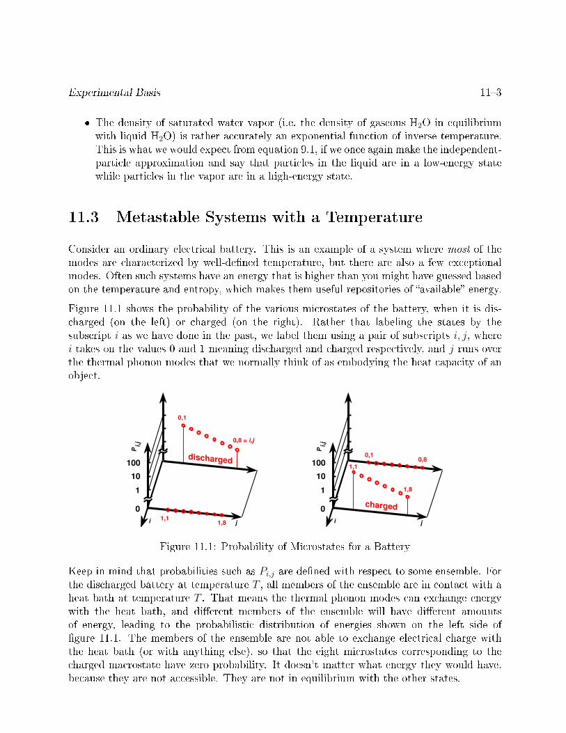
Experimental Basis 113

The density of saturated water vapor (i.e. the density of gaseous H2O in equilibriumwith liquid H2O) is rather accurately an exponential function of inverse temperature.This is what we would expect from equation 9.1, if we once again make the independent-particle approximation and say that particles in the liquid are in a low-energy statewhile particles in the vapor are in a high-energy state.

11.3 Metastable Systems with a Temperature

Consider an ordinary electrical battery. This is an example of a system where most of themodes are characterized by well-dened temperature, but there are also a few exceptionalmodes. Often such systems have an energy that is higher than you might have guessed basedon the temperature and entropy, which makes them useful repositories of available energy.

Figure 11.1 shows the probability of the various microstates of the battery, when it is dis-charged (on the left) or charged (on the right). Rather that labeling the states by thesubscript i as we have done in the past, we label them using a pair of subscripts i, j, wherei takes on the values 0 and 1 meaning discharged and charged respectively, and j runs overthe thermal phonon modes that we normally think of as embodying the heat capacity of anobject.

0,1

1,11,8

Pi,j

10

100

1

0

0,8 = i,j

j

10

100

1

0

1,1

1,8

0,10,8

i j i

Pi,j

discharged

charged

Figure 11.1: Probability of Microstates for a Battery

Keep in mind that probabilities such as Pi,j are dened with respect to some ensemble. Forthe discharged battery at temperature T , all members of the ensemble are in contact with aheat bath at temperature T . That means the thermal phonon modes can exchange energywith the heat bath, and dierent members of the ensemble will have dierent amountsof energy, leading to the probabilistic distribution of energies shown on the left side ofgure 11.1. The members of the ensemble are not able to exchange electrical charge withthe heat bath (or with anything else), so that the eight microstates corresponding to thecharged macrostate have zero probability. It doesn't matter what energy they would have,because they are not accessible. They are not in equilibrium with the other states.


Meanwhile, on the right side of the gure, the battery is in the charged state. The eightmicrostates corresponding to the discharged macrostate have zero probability, while the eightmicrostates corresponding to the charged macrostate have a probability distribution of theexpected Boltzmann form.

Comparing the left side with the right side of gure 11.1, we see that the two batteries havethe same temperature. That is, the slope of log(Pi,j) versus Ei,j for the modes that areactually able to contribute to the heat capacity is the same for the two batteries.

You may be wondering how we can reconcile the following four facts: (a) The two batterieshave the same temperature T , (b) the accessible states of the two batteries have dierentenergies, indeed every accessible state of the charged battery has a higher energy than anyaccessible state of the discharged battery, (c) corresponding accessible states of the twobatteries have the same probabilities, and (d) both batteries obey the Boltzmann law, Pi,jproportional to exp(−Ei,j/kT ). The answer is that there is a bit of a swindle regarding themeaning of proportional. The discharged battery has one proportionality constant, whilethe charged battery has another. For details on this, see section 24.1.

Here is a list of systems that display this sort of separation between thermal modes andnonthermal modes:• an electrochemical storage battery that may have a shelf life of ten months or ten years.• a ywheel that may keep spinning for one second or one hour or one day.• a large piece of metal that rings like a bell, i.e. with a high excitation in one of itsmechanical resonance modes.• a capacitor that may hold its charge for hours or days.• a uid-dynamic excitation such as the wingtip vortices trailing behind an airplane.• a weight-driven cuckoo clock that may go a day or a week between windings.• a spring-driven clock that may go a day or a week or a year between windings.• a microwave oven that puts potato-molecules into an excited state.• a metastable chemical species such as H2O2 or TNT. If left to themselves, they willdecompose quickly or slowly, depending on temperature, catalysis, and other details.• a classical Carnot-cycle heat engine. If you operate it too quickly, there will be nonide-alities because the parts of the cycle that are supposed to be isothermal won't be (i.e.the working uid won't be in good thermal contact with the heat bath). On the otherhand, if you operate it too slowly, there will be nonidealities due to parasitic thermalconduction through structures such as the pushrod that connects the piston to theload. You cannot assume or postulate that there is a nice big separation between thetoo-slow timescale and the too-fast timescale; if you need a big separation you mustarrange for it by careful engineering.

(Section 11.4 takes another look at metastable systems.)

There are good reasons why we might want to apply thermodynamics to systems such asthese. For instance, the Clausius-Clapeyron equation can tell us interesting things about avoltaic cell.


Also, just analyzing such a system as a Gedankenexperiment helps us understand a thing ortwo about what we ought to mean by equilibrium, temperature, heat, and work.

In equilibrium, the accessible states are supposed to be occupied in accordance with theBoltzmann distribution law (equation 9.1).

An example is depicted in gure 11.1, which is a scatter plot of Pi,j versus Ei,j.

As mentioned in section 10.1, Feynman dened equilibrium to be when all the fast thingshave happened but the slow things have not (reference 28). The examples listed at thebeginning of this section all share the property of having two timescales and therefore twonotions of equilibrium. If you charge up such a system you create a Boltzmann distributionwith exceptions. There are not just a few exceptions as in gure 11.3, but huge classes ofexceptions, i.e. huge classes of microstates that are (in the short run, at least) inaccessible.If you revisit the system on longer and longer timescales, eventually the energy may becomedissipated into the previously-inaccessible states. For example, the battery may self-dischargevia some parasitic internal conduction path.

Ei

ilo

g(

)

P

ilo

g(

)

P

Ei

Figure 11.2: An Equilibrium DistributionFigure 11.3: An Equilibrium Distributionwith Exceptions

The idea of temperature is valid even on the shorter timescale. In practice, I can measurethe temperature of a battery or a ywheel without waiting for it to run down. I can measurethe temperature of a bottle of H2O2 without waiting for it to decompose.

This proves that in some cases of interest, we cannot write the system energy E as a functionof the macroscopic thermodynamic variables V and S. Remember, V determines the spacingbetween energy levels (which is the same in both gures) and S tells us something aboutthe occupation of those levels, but alas S does not tell us everything we need to know. Anelementary example of this can be seen by comparing gure 9.1 with gure 11.3, where wehave the same V , the same S, and dierent E. So we must not assume E = E(V, S). Amore spectacular example of this can be seen by comparing the two halves of gure 11.1.

Occasionally somebody tries to argue that the laws of thermodynamics do not apply togure 11.3 or gure 11.1, on the grounds that thermodynamics requires strict adherenceto the Boltzmann exponential law. This is a bogus argument for several reasons. First ofall, strict adherence to the Boltzmann exponential law would imply that everything in sight

was at the same temperature. That means we can't have a heat engine, which depends onhaving two heat reservoirs at dierent temperatures. A theory of pseudo-thermodynamicsthat cannot handle exceptions to the Boltzmann exponential law is useless.

So we must allow some exceptions to the Boltzmann exponential law . . . maybe not everyimaginable exception, but some exceptions. A good criterion for deciding what sort of


exceptions to allow is to ask whether it is operationally possible to measure the temperature.For example, in the case of a storage battery, it is operationally straightforward to designa thermometer that is electrically insulated from the exceptional mode, but thermally wellconnected to the thermal modes.

Perhaps the most important point is that equation 1.1 and equation 2.1 apply directly,without modication, to the situations listed at the beginning of this section. So from thispoint of view, these situations are not exceptional at all.

The examples listed at the beginning of this section raise some other basic questions. SupposeI stir a large tub of water. Have I done work on it (w) or have I heated it (q)? If the questionis answerable at all, the answer must depend on timescales and other details. A big vortexcan be considered a single mode with a huge amount of energy, i.e. a huge exception to theBoltzmann distribution. But if you wait long enough the vortex dies out and you're leftwith just an equilibrium distribution. Whether you consider this sort of dissipation to beq and/or heat is yet another question. (See section 7.10 and especially section 17.1 for adiscussion of what is meant by heat.)

In cases where the system's internal spin-down time is short to all other timescales ofinterest, we get plain old dissipative systems. Additional examples include:• The Rumford experiment (section 11.5.3).• Shear in a viscous uid (section 11.5.5).• A block sliding down an inclined plane, under the inuence of sliding friction.• The brake shoes on a car.• et cetera.

11.4 Metastable Systems without a Temperature

An interesting example is:• a three-state laser, in which there is a population inversion.

In this case, it's not clear how to measure the temperature or even dene the temperatureof the spin system. Remember that in equilibrium, states are supposed to be occupiedwith probability proportional to the Boltzmann factor, Pi ∝ exp(−Ei/kT ). However, themiddle microstate is more highly occupied than the microstates on either side, as depicted ingure 11.4. This situation is clearly not describable by any exponential, since exponentialsare monotone.

We cannot use the ideas discussed in section 11.3 to assign a temperature to such a system,because it has so few states that we can't gure out which ones are the thermal backgroundand which ones are the exceptions.

Such a system does have an entropy even though it doesn't have a temperature, even thoughit is metastable, and even though it is grossly out of equilibrium. It is absolutely crucial


ilo

g(

)

P

Ei

Figure 11.4: Three-State System without a Temperature

that the system system have a well-dened entropy, for reasons suggested by gure 11.5.That is, suppose the system starts out in equilibrium, with a well-dened entropy S(1).It then passes through in intermediate state that is out of equilibrium, and ends up in anequilibrium state with entropy S(3). The law of paraconservation of entropy is meaninglessunless we can somehow relate S(3) to S(1). The only reasonable way that can happen is ifthe intermediate state has a well-dened entropy. The intermediate state typically does nothave a temperature, but it does have a well-dened entropy.

Equilibrium Equilibrium Out OfEquilibrium

S(1) ??? S(3)

Figure 11.5: Non-Equilibrium: Well-Dened Entropy

11.5 Dissipative Systems

11.5.1 Sudden Piston : Sound

Consider the apparatus shown in gure 11.6. You can consider it a two-sided piston.

Equivalently you can consider it a loudspeaker in an unusual full enclosure. (Loudspeakersare normally only half-enclosed.) It is roughly like two unported speaker enclosures face toface, completely enclosing the speaker driver that sits near the top center, shown in red. Theinterior of the apparatus is divided into two regions, 1 and 2, with time-averaged properties(E1, S1, T1, P1, V1) and (E2, S2, T2, P2, V2) et cetera. When the driver (aka piston) moves tothe right, it increase volume V1 and decreases volume V2. The box as a whole is thermallyisolated / insulated / whatever. That is to say, no entropy crosses the boundary. No energycrosses the boundary except for the electricity feeding the speaker.


1 2

b

Figure 11.6: Two-Sided Piston


You could build a simplied rectangular version of this apparatus for a few dollars. Itis considerably easier to build and operate than Rumford's cannon-boring apparatus (sec-tion 11.5.3).

We will be primarily interested in a burst of oscillatory motion. That is, the piston is initiallyat rest, then oscillates for a while, and then returns to rest at the original position.

When the piston moves, it does F · dx work against the gas. There are two contributions.Firstly, the piston does work against the gas in each compartment. If P1 = P2 this contri-bution vanishes to rst order in dV . Secondly, the piston does work against the pressure inthe sound eld.

The work done against the average pressure averages to zero over the course of one cycle ofthe oscillatory motion ... but the work against the radiation eld does not average to zero.The dV is oscillatory but the eld pressure is oscillatory too, and the product is positive onaverage.

The acoustic energy radiated into the gas is in the short term not in thermal equilibrium withthe gas. In the longer term, the sound waves are damped i.e. dissipated by internal frictionand also by thermal conductivity, at a rate that depends on the frequency and wavelength.

What we put in is F · dx (call it work if you wish) and what we get out in the long run isan increase in the energy and entropy of the gas (call it heat if you wish).

It must be emphasized that whenever there is appreciable energy in the sound eld, it is notpossible to write E1 as a function of V1 and S1 alone, or indeed to write E1 as a function ofany two variables whatsoever. In general, the sound creates a pressure P (r) that varies fromplace to place as a function of the position-vector r. That's why we call it a sound eld; it'sa scalar eld, not a simple scalar.

As a consequence, when there is appreciable energy in the sound eld, it is seriously incorrectto expand dE = T dS − P dV . The correct expansion necessarily has additional termson the RHS. Sometimes you can analyze the sound eld in terms of its normal modes,and in some simple cases most of the sound energy resides in only a few of the modes,in which case you need only a few additional variables. In general, though, the pressurecan vary from place to place in an arbitrarily complicated way, and you would need anarbitrarily large number of additional variables. This takes us temporarily outside the scopeof ordinary thermodynamics, which requires us to describe the macrostate as a function ofsome reasonably small number of macroscopic variables. The total energy, total entropy,and total volume are still perfectly well dened, but they do not suce to give a completedescription of what is going on. After we stop driving the piston, the sound waves willeventually dissipate, whereupon we will once again be able to describe the system in termsof a few macroscopic variables.

If the piston moves slowly, very little sound will be radiated and the process will be essentiallyisentropic and reversible. On the other hand, if the piston moves quickly, there will be lots of


sound, lots of dissipation, and lots of newly created entropy. This supports the point madein section 10.2: timescales matter.

At no time is any entropy transferred across the boundary of the region. The increase inentropy of the region is due to new entropy, created from scratch in the interior of the region.

If you want to ensure the gas exerts zero average force on the piston, you can cut a small holein the bae near point b. Then the only work the piston can do on the gas is work againstthe sound pressure eld. There is no longer any important distinction between region 1 andregion 2.

You can even remove the bae entirely, resulting in the racetrack apparatus shown ingure 11.7.

The kinetic energy of the piston is hardly worth worrying about. When we say it takesmore work to move the piston rapidly than slowly, the interesting part is the work doneon the gas, not the work done to accelerate the piston. Consider a very low-mass piston ifthat helps. Besides, whatever KE goes into the piston is recovered at the end of each cycle.Furthermore, it is trivial to calculate the F · dx of the piston excluding whatever force isnecessary to accelerate the piston. Let's assume the experimenter is clever enough to applythis trivial correction, so that we know, moment by moment, how much F · dx work isbeing done on the gas. This is entirely conventional; the conventional pressures P1 and P2

are associated with the forces F1 and F2 on the faces of the piston facing the gas, not theforce Fd that is driving the piston. To relate Fd to F1 and F2 you would need to considerthe mass of the piston, but if you formulate the problem in terms of F1 · dx and F2 · dx, asyou should, questions of piston mass and piston KE should hardly even arise.

11.5.2 Sudden Piston : State Transitions

Let's forget about all the complexities of the sound eld discussed in section 11.5.1. Insteadlet's take the quantum mechanical approach. Let's simplify the gas down to a single particle,the familiar particle in a box, and see what happens.

As usual, we assume the box is rigid and thermally isolated / insulated / whatever. Noentropy ows across the boundary of the box. Also, no energy ows across the boundaryexcept for the work done by the piston.

Since we are interested in entropy, it will not suce to talk about the quantum stateof the particle. The entropy of any particular quantum state (microstate) is zero. We canhowever represent the thermodynamic state (macrostate) using a density matrix ρ. For somebackground on density matrices in the context of thermodynamics, see chapter 27.

The entropy is given by equation 27.6. which is the gold-standard most-general denition ofentropy; in the classical limit it reduces to the familiar workhorse expression equation 2.2


Figure 11.7: Racetrack with Piston


For simplicity we consider the case where the initial state is a pure state, i.e. a single mi-crostate. That means the initial entropy is zero, as you can easily verify. Hint: equation 27.6is particularly easy to evaluate in a basis where ρ is diagonal.

Next we perturb our particle-in-a-box by moving one wall of the box inward. We temporarilyassume this is done in such a way that the particle ends up in the same microstate. Thatis, the nal state is identical to the original quantum state except for the shorter wavelengthas required to t into the smaller box. It is a straightforward yet useful exercise to showthat this does P dV work on the particle. The KE of the new state is higher than the KEof the old state.

Now the fun begins. We retract the previous assumption about the nal state; insteadwe calculate the nal macrostate using perturbation theory. In accordance with Fermi'sgolden rule we calculate the overlap integral between the original quantum state (originalwavelength) and each of the possible nal quantum states (slightly shorter wavelength).

Each member of the original set of basis wavefunctions is orthogonal to the other members.The same goes for the nal set of basis wavefunctions. However, each nal basis wavefunctionis only approximately orthogonal to the various original basis wavefunctions. So the previousassumption that the particle would wind up in the corresponding state is provably not quitetrue; when we do the overlap integrals there is always some probability of transition tonearby states.

It is straightforward to show that if the perturbation is slow and gradual, the correspondingstate gets the lion's share of the probability. Conversely, if the perturbation is large andsudden, there will be lots of state transitions. The nal state will not be a pure quantumstate. It will be a mixture. The entropy will be nonzero, i.e. greater than the initial entropy.

To summarize:slow and gradual =⇒ isentropic, non dissipativesudden =⇒ dissipative

So we are on solid grounds when we say that in a thermally isolated cylinder, a gradualmovement of the piston is isentropic, while a sudden movement of the piston is dissipative.Saying that the system is adiabatic in the sense of thermally insulated does not suce tomake it adiabatic in the sense of isentropic.

Note that in the quantum mechanics literature the slow and gradual case is conventionallycalled the adiabatic approximation in contrast to the sudden approximation. Theseterms are quite rmly established ... even though it conicts with the also well-establishedconvention in other branches of physics where adiabatic means thermally insulated; seenext message.

There is a nice introduction to the idea of radiation resistance in reference 8 chapter 32.


11.5.3 Rumford's Experiment

Benjamin Thompson (Count Rumford) did some experiments that were published in 1798.Before that time, people had more-or-less assumed that heat by itself was conserved. Rum-ford totally demolished this notion, by demonstrating that unlimited amounts of heat couldbe produced by nonthermal mechanical means. Note that in this context, the terms thermalenergy, heat content, and caloric are all more-or-less synonymous ... and I write each ofthem in scare quotes.

From the pedagogical point of view Rumford's paper is an optimal starting point; the exam-ples in section 11.5.1 and section 11.5.2 are probably better. For one thing, a microscopicunderstanding of sound and state-transitions in a gas is easier than a microscopic under-standing of metal-on-metal friction.

Once you have a decent understanding of the modern ideas, you would do well to readRumford's original paper, reference 30. The paper is of great historical importance. It iseasy to read, informative, and entertaining. On the other hand, beware that it contains atleast one major error, plus one trap for the unwary:

The title is wrong and the bottom-line conclusion is wrong, for reasons discussed insection 9.3.3.

The analysis depends on a cramped notion of heat content that is more-or-less OK inthis particular context, but is not clearly dened, and but would cause serious problemsif you tried to extend it to uncramped thermodynamics.

The main point of the paper is that heat is not conserved. This point remains true andimportant. The fact that the paper has a couple of bugs does not detract from this point.

You should reect on how something can provide valuable (indeedepochal) information and still not be 100% correct.

All too often, the history of science is presented as monotonic progressbuilding one pure success upon another, but this is not how thingsreally work. In fact there is a lot of back-tracking out of dead ends.Real science and real life are like football, in the sense that any playthat advances the ball 50 or 60 yards it is a major accomplishment,even if you get knocked out of bounds before reaching the ultimategoal. Winning is important, but you don't need to win the entiregame, single handedly, the rst time you get your hands on the ball.

Rumford guessed that all the heat capacity was associated with motion because hecouldn't imagine anything else. It was a process-of-elimination argument, and he blew it.This is understandable, given what he had to work with.


A hundred years later, guys like Einstein and Debye were able to cobble up a theory of heatcapacity based on the atomic model. We know from this model that the heat capacity ofsolids is half kinetic and half potential. Rumford didn't stand much of a chance of guringthis out.

It is possible to analyze Rumford's experiment without introducing the notion of heatcontent. It suces to keep track of the energy and the entropy. The energy can be quanti-ed by using the rst law of thermodynamics, i.e. the conservation of energy. We designatethe cannon plus the water bath as the system of interest. We know how much energywas pushed into the system, pushed across the boundary of the system, in the form ofmacroscopic mechanical work. We can quantify the entropy by means of equation 7.21, i.e.dS = (1/T )dE at constant pressure. Energy and entropy are functions of state, even insituations where heat content is not.

Heat is a concept rooted in cramped thermodynamics, and causes serious trouble if you tryto extend it to uncramped thermodynamics. Rumford got away with it, in this particularcontext, because he stayed within the bounds of cramped thermodynamics. Specically, hedid everything at constant pressure. He used the heat capacity of water at constant pressureas his operational denition of heat content.

To say the same thing the other way, if he had strayed o the contour of constantP , perhaps by making little cycles in the PV plane, using the water as theworking uid in a heat engine, any notion of heat content would have gone outthe window. There would have been an unholy mixture of CP and CV , and theheat content would have not been a function of state, and everybody wouldhave been sucked down the rabbit-hole into crazy-nonsense land.

We note in passing that it would be impossible to reconcile Rumford's notion of heat withthe various other notions listed in section 17.1 and section 18.1. For example: work is beingdone in terms of energy owing across the boundary, but no work is being done in terms ofthe work/KE theorem, since the cannon is not accelerating.

For more about the diculties in applying the work/KE theorem to thermodynamic ques-tions, see reference 18.

We can begin to understand the microscopics of sliding friction using many of the same ideasas in section 11.5.1. Let's model friction in terms of asperities on each metal surface. Eachof the asperities sticks and lets go, sticks and lets go. When it lets go it wiggles and radiatesultrasound into the bulk of the metal. This produces in the short term a nonequilibriumstate due to the sound waves, but before long the sound eld dissipates, depositing energyand creating entropy in the metal.

Again, if you think in terms only of the (average force) dot (average dx) you will neverunderstand friction or dissipation. You need to model many little contributions of the form


(short term force) dot (short term dx) and then add up all the contributions. This is whereyou see the work being done against the radiation eld.

At ordinary temperatures (not too hot and not too cold) most of the heat capacity in asolid is associated with the phonons. Other phenomena associated with friction, includingdeformation and abrasion of the materials, are only very indirectly connected to heating.Simply breaking a bunch of bonds, as in cleaving a crystal, does not produce much in theway of entropy or heat. At some point, if you want to understand heat, you need to coupleto the phonons.

11.5.4 Simple Example: Decaying Current

Suppose we have some current I owing in a wire loop, as shown in gure 11.8. Thecurrent will gradually decay, on a timescale given by L/R, i.e. the inductance divided by theresistance.

The temperature of the wire will increase, and the entropy of the wire will increase, eventhough no energy is being transferred (thermally or otherwise) across the boundary of thesystem.

(Even if you consider an imaginary boundary between the conduction electrons and the restof the metal, you cannot possibly use any notion of energy owing across the boundary toexplain the fact that both subsystems heat up.)

A decaying current of water in an annular trough can be used to make the same point.

11.5.5 Simple Example: Oil Bearing

Here is a modied version of Rumford's experiment, more suitable for quantitative analysis.Note that reference 31 carries out a similar analysis and reaches many of the same conclusions.Also note that this can be considered a macroscopic mechanical analog of the NMR τ2 process,where there is a change in entropy with no change in energy. See also gure 1.3.

Suppose we have an oil bearing as shown in gure 11.9. It consists of an upper plate and alower plate, with a thin layer of oil between them. Each plate is a narrow annulus of radiusR. The lower plate is held stationary. The upper plate rotates under the inuence of a forceF , applied via a handle as shown. The upper plate is kept coaxial with the lower plate by aforce of constraint, not shown. The two forces combine to create a pure torque, τ = F/R.The applied torque τ is balanced in the long run by a frictional torque τ ′; specically

〈τ〉 = 〈τ ′〉 (11.2)

where 〈. . .〉 denotes a time-average. As another way of saying the same thing, in the longrun the upper plate settles down to a more-or-less steady velocity.



I

Figure 11.8: Current in a Wire Loop

RF

Figure 11.9: Oil Bearing


We arrange that the system as a whole is thermally insulated from the environment, to asucient approximation. This includes arranging that the handle is thermally insulating. Inpractice this isn't dicult.

We also arrange that the plates are somewhat thermally insulating, so that heat in the oildoesn't immediately leak into the plates.

Viscous dissipation in the oil causes the oil to heat up. To a good approximation this is theonly form of dissipation we must consider.

In an innitesimal period of time, the handle moves through a distance dx or equivalentlythrough an angle dθ = dx/R. We consider the driving force F to be a controlled variable.We consider θ to be an observable dependent variable. The relative motion of the plates setsup a steady shearing motion within the oil. We assume the oil forms a suciently thin layerand has suciently high viscosity that the ow is laminar (i.e. non-turbulent) everywhere.We say the uid has a very low Reynolds number (but if you don't know what that means,don't worry about it). The point is that the velocity of the oil follows the simple patternshown by the red arrows in gure 11.10.

Lower plate

Upper plate

Oil

Figure 11.10: Shear: Velocity Field in the Oil

The local work done on the handle by the driving force is w = Fdx or equivalently w = τdθ.This tells us how much energy is owing across the boundary of the system. From now on westop talking about work, and instead talk about energy, condent that energy is conserved.

We can keep track of the energy-content of the system by integrating the energy inputs.Similarly, given the initial entropy and the heat capacity of the materials, we can predict theentropy at all times1 by integrating equation 7.14. Also given the initial temperature andheat capacity, we can predict the temperature at all times by integrating equation 7.13. Wecan then measure the temperature and compare it with the prediction.

1If the ow pattern were turbulent, calculating the entropy would entail practical as well as conceptualdiculties.


We can understand the situation in terms of equation 1.1. Energy τdθ comes in via thehandle. This energy cannot be stored as potential energy within the system. This energyalso cannot be stored as macroscopic or mesoscopic kinetic energy within the system, sinceat each point the velocity is essentially constant. By a process of elimination we concludethat this energy accumulates inside the system in microscopic form.

This gives us a reasonably complete description of the thermodynamics of the oil bearing.

This example is simple, but helps make a very important point. If you base your thermo-dynamics on wrong foundations, it will get wrong answers, including the misconceptionsdiscussed in section 11.5.6 and section 11.5.7.

Some people who use wrong foundations try to hide from the resulting problems narrowingtheir denition of thermodynamics so severely that it has nothing to say right or wrong about dissipative systems. Making no predictions is a big improvement over making wrongpredictions . . . but still it is a terrible price to pay. Real thermodynamics has tremendouspower and generality. Real thermodynamics applies just ne to dissipative systems. Seechapter 21 for more on this.

11.5.6 Misconceptions : Heat

There are several correct ways of analyzing the oil-bearing system, one of which was presentedin section 11.5.5. In addition, there are innumerably many incorrect ways of analyzing things.We cannot list all possible misconceptions, let alone discuss them all. However, it seemsworthwhile to point out some of the most prevalent pitfalls.

You may have been taught to think of heating in terms of the thermal transfer of energyacross a boundary. If you're going to use that denition, you must keep in mind that it is notequivalent to the TdS denition. In other words, in section 17.1, denition #5 is sometimesvery dierent from denition #2. The decaying current in section 11.5.4 and the oil-bearingexample in section 11.5.5 clearly demonstrates this dierence.

Among other things, this dierence can be seen as another instance of boundary/interiorinconsistency, as discussed in section 8.6. Specically:

No heat is owing into the oil. The oil ishotter than its surroundings, so if there isany heat-ow at all, it ows outward fromthe oil.

The TdS/dt is strongly positive. The en-tropy of the oil is steadily increasing.

Another point that can be made using this example is that the laws of thermodynamics applyjust ne to dissipative systems. Viscous damping has a number of pedagogical advantagesrelative to (say) the sliding friction in Rumford's cannon-boring experiment. It's clear wherethe dissipation is occurring, and it's clear that the dissipation does not prevent us fromassigning a well-behaved temperature to each part of the apparatus. Viscous dissipation is


more-or-less ideal in the sense that it does not depend on submicroscopic nonidealities suchas the asperities that are commonly used to explain solid-on-solid sliding friction.

11.5.7 Misconceptions : Work

We now discuss some common misconceptions about work.

Work is susceptible to boundary/interior inconsistencies for some of the same reasons thatheat is.

You may have been taught to think of work as an energy transfer across a boundary. That'sone of the denitions of work discussed in section 18.1. It's often useful, and is harmlessprovided you don't confuse it with the other denition, namely PdV .

Work-ow is the work that shows up inthe principle of virtual work (reference 32),e.g. when we want to calculate the force onthe handle of the oil bearing.

Work-PdV is the work that shows up inthe work/KE theorem.

11.5.8 Remarks

This discussion has shed some light on how equation 7.5 can and cannot be interpreted.• Sometimes the terms on the RHS are well-dened and can be interpreted as workand heat.• Sometimes the terms on the RHS are well-dened but do not correspond to conventionalnotions of work and heat.• Sometimes the terms on the RHS are not even well-dened, i.e. the derivatives do notexist.

In all cases, the equation should not be considered the rst law of thermodynamics, becauseit is inelegant and in every way inferior to a simple, direct statement of local conservation ofenergy.

11.6 The Gibbs Gedankenexperiment

As shown in gure 11.11, suppose we have two moderate-sized containers connected by avalve. Initially the valve is closed. We ll one container with an ideal gas, and ll the othercontainer with a dierent ideal gas, at the same temperature and pressure. When we openthe valve, the gases will begin to mix. The temperature and pressure will remain unchanged,but there will be an irreversible increase in entropy. After mixing is complete, the molarentropy will have increased by R ln 2.


Figure 11.11: The Gibbs Gedankenexperiment

As Gibbs observed,2 the R ln 2 result is independent of the choice of gases, . . . except thatthe gases which are mixed must be of dierent kinds. If we should bring into contact twomasses of the same kind of gas, they would also mix, but there would be no increase ofentropy.

There is no way to explain this in terms of 19th-century physics. The explanation depends onquantum mechanics. It has to do with the fact that one helium atom is identical (absolutelytotally identical) with another helium atom.

Also consider the following contrast:

In gure 11.11, the pressure on both sidesof the valve is the same. There is no netdriving force. The process proceeds by dif-fusion, not by macroscopic ow.

This contrasts with the scenario where wehave gas on one side of the partition, butvacuum on the other side. This is dra-matically dierent, because in this scenariothere is a perfectly good 17th-century dy-namic (not thermodynamic) explanationfor why the gas expands: there is a pres-sure dierence, which drives a ow of uid.

Entropy drives the process. There is nohope of extracting energy from the diu-sive mixing process.

Energy drives the process. We could ex-tract some of this energy by replacing thevalve by a turbine.

The timescale for free expansion is roughly L/c, where L is the size of the apparatus, andc is the speed of sound. The timescale for diusion is slower by a huge factor, namely by afactor of L/λ, where λ is the mean free path in the gas.

Pedagogical note: The experiment in gure 11.11 is not very exciting to watch.Here's an alternative: Put a drop or two of food coloring in a beaker of stillwater. The color will spread throughout the container, but only rather slowly.This allows students to visualize a process driven by entropy, not energy.

Actually, it is likely that most of the color-spreading that you see is due toconvection, not diusion. To minimize convection, try putting the water in atall, narrow glass cylinder, and putting it under a Bell jar to protect it fromdrafts. Then the spreading will take a very long time indeed.

2Quoted in reference 33.


Beware: Diusion experiments of this sort are tremendously valuable if explained properly. . . but they are horribly vulnerable to misinterpretation if not explained properly, for reasonsdiscussed in section 9.9.

For a discussion of the microscopic theory behind the Gibbs mixing experiments, see sec-tion 26.2.

11.7 Spin Echo Experiment

It is possible to set up an experimental situation where there are a bunch of nuclei whose spinsappear to be oriented completely at random, like a well-shued set of cards. However, if Ilet you in on the secret of how the system was prepared, you can, by using a certain sequenceof Nuclear Magnetic Resonance (NMR) pulses, get all the spins to line up evidently a verylow-entropy conguration.

The trick is that there is a lot of information in the lattice surrounding the nuclei, some-thing like 1023 bits of information. I don't need to communicate all this information to youexplicitly; I just need to let you in on the secret of how to use this information to untanglethe spins.

The ramications and implications of this are discussed in section 12.8.

11.8 Melting

Take a pot of ice water. Add energy to it via friction, à la Rumford, as described in sec-tion 11.5.3. The added energy will cause the ice to melt. The temperature of the ice waterwill not increase, not until all the ice is gone.

This illustrates the fact that temperature is not the same as thermal energy. It focuses ourattention on the entropy. A gram of liquid water has more entropy than a gram of ice. Soat any given temperature, a gram of water has more energy than a gram of ice.

The following experiment makes an interesting contrast.

11.9 Isentropic Expansion and Compression

Take an ideal gas acted upon by a piston. For simplicity, assume a nonrelativistic nondegen-erate ideal gas, and assume the sample is small on the scale of kT/mg. Assume everythingis thermally insulated, so that no energy enters or leaves the system via thermal conduction.


Gently retract the piston, allowing the gas to expand. The gas cools as it expands. In theexpanded state,

• The gas has essentially the same entropy, if the expansion was done gently enough.

• The gas has a lower temperature.

• The gas has less energy, by some amount ∆E.

Before the expansion, the energy in ques-tion (∆E) was in microscopic Locrianform, within the gas.

After the expansion, this energy is inmacroscopic non-Locrian form, within themechanism that moves the piston.

This scenario illustrates some of the dierences between temperature and entropy, and someof the dierences between energy and entropy.

Remember, the second law of thermodynamics says that the entropy obeys a local law ofparaconservation. Be careful not to misquote this law.

It doesn't say that the temperature can'tdecrease. It doesn't say that the so-calledthermal energy can't decrease.

It says the entropy can't decrease in anygiven region of space, except by owinginto adjacent regions.

Energy is conserved. That is, it cannot increase or decrease except by owing into adjacentregions. (You should not imagine that there is any law that says thermal energy by itselfis conserved.)

If you gently push the piston back in, compressing the gas, the temperature will go back up.

Isentropic compression is an increase in temperature at constant entropy. Melting (sec-tion 11.8) is an increase in entropy at constant temperature. These are two radically dierentways of increasing the energy.

11.10 Demagnetization Refrigerator

Obtain (or construct) a simple magnetic compass. It is essentially a bar magnet that is freeto pivot. Attach it to the middle of a board. By placing some small magnets elsewhere onthe board, you should (with a little experimentation) be able to null out the earth's eldand any other stray elds, so that the needle rotates freely. If you don't have convenientphysical access to the needle, you can set it spinning using another magnet.

Note: The earth's eld is small, so it doesn't take much to null it out. You can make yourown not-very-strong magnets by starting with a piece of steel (perhaps a sewing pin) andmagnetizing it.

Once you have a freely-moving needle, you can imagine that if it were smaller and morenely balanced, thermal agitation would cause it to rotate randomly back and forth forever.


Now hold another bar magnet close enough to ruin the free rotation, forcing the spinner toalign with the imposed eld.

This is a passable pedagogical model of the guts of a demagnetization refrigerator. Suchdevices are routinely used to produce exceedingly low temperatures, within a millionth of adegree of absolute zero. Copper nuclei can be used as the spinners.

At low temperatures in a high magnetic eld, the copper nuclei have only one accessiblestate. This corresponds to zero molar entropy.

At high temperatures in a low magnetic eld, the nuclei are free and have 4 equiprobablestates. The 4 arises because both kinds of naturally-occurring copper nuclei have totalspin I = 3/2, so there are four possible mI values, namely +3/2, +1/2, −1/2, and−3/2. This corresponds to a molar entropy of s = R ln(4). All the other quantumnumbers are irrelevant; the four mI states are the only accessible states.

The compass is not a perfect model of the copper nucleus, insofar as it has more than fourstates when it is spinning freely. However, if you use your imagination, you can pretendthere are only four states. When a strong eld is applied, only one of these states remainsaccessible.

It is worthwhile to compare theory to experiment:

These values for the molar entropy s havea rm theoretical basis. They require littlemore than counting. We count microstatesand apply the denition of entropy. Thenwe obtain ∆s by simple subtraction.

Meanwhile, ∆s can also obtained experi-mentally, by observing the classical macro-scopic thermodynamic behavior of the re-frigerator.

Both ways of obtaining ∆s give the same answer. What a coincidence! This answers thequestion about how to connect microscopic state-counting to macroscopic thermal behavior.The Shannon entropy is not merely analogous to the thermodynamic entropy; it is thethermodynamic entropy.

Spin entropy is discussed further in section 12.4.

Tangential remark: There are some eorts devoted to using demagnetization to producerefrigeration under conditions that are not quite so extreme; see e.g. reference 34.

11.11 Thermal Insulation

As a practical technical matter, it is often possible to have a high degree of thermal insulationbetween some objects, while other objects are in vastly better thermal contact.


For example, if we push on an object using a thermally-insulating stick, we can transferenergy to the object, without transferring much entropy. In contrast, if we push on a hotobject using a non-insulating stick, even though we impart energy to one or two of theobject's modes by pushing, the object could be losing energy overall, via thermal conductionthrough the stick.

Similarly, if you try to build a piece of thermodynamic apparatus, such as an automobileengine, it is essential that some parts reach thermal equilibrium reasonably quickly, and itis equally essential that other parts do not reach equilibrium on the same timescale.

Chapter 12

More About Entropy

12.1 Terminology: Microstate versus Macrostate

Beware: In the thermodynamics literature, the word state is used with two inconsistentmeanings. It could mean either microstate or macrostate.

In a system such as the deck of cards dis-cussed in section 2.3, the microstate isspecied by saying exactly which card ison top, exactly which card is in the secondposition, et cetera.

In that system, the macrostate is the en-semble of all card decks consistent withwhat we know about the situation.

In a system such as a cylinder of gas, a mi-crostate is a single fully-specied quantumstate of the gas.

For such a gas, the macrostate is speciedby macroscopic variables such as the tem-perature, density, and pressure.

In general, a macrostate is an equivalenceclass, i.e. a set containing some numberof microstates (usually many, many mi-crostates).

In the context of quantum mechanics, statealways means microstate.

In the context of classical thermodynam-ics, state always means macrostate, for in-stance in the expression function of state.

The idea of microstate and the idea of macrostate are both quite useful. The problem ariseswhen people use the word state as shorthand for one or both. You can get away withstate=microstate in introductory quantum mechanics (no thermo), and you can get awaywith state=macrostate in introductory classical thermo (no quantum mechanics) . . . butthere is a nasty collision as soon as you start doing statistical mechanics, which sits astridethe interface between QM and thermo.


In this document, the rule is that statemeans microstate, unless the context re-quires otherwise.

When we mean macrostate, we explic-itly say macrostate or thermodynamicstate. The idiomatic expression functionof state necessarily refers to macrostate.

The relationship between microstate and macrostate, and their relationship to entropy, isdiscussed in section 2.7 and section 12.1.

Also, chapter 20 is a tangentially-related discussion of other inconsistent terminology.

12.2 What the Second Law Doesn't Tell You

Remember that the entropy is a property of the macrostate, not of any particular microstate.The macrostate is an ensemble of identically-prepared systems.

Therefore, if you are studying a single system, the second law doesn't necessarily tell youwhat that system is going to do. It tells you what an ensemble of such systems would do, butthat's not necessarily the same thing. At this point there are several options. The ensembleaverage is the strongly recommended option.

1. For a large system, you may be able to use your imagination to divide the systeminto many pieces, so that you have an ensemble of pieces. Each of the N pieces is inequilibrium with a heat bath consisting of the other N − 1 pieces. You can take theaverage over pieces and (maybe) substitute it for the ensemble average.

You must assume the system is homogeneous, or do a lot of extra work to accountfor any inhomogeneity.

This throws the baby out with the bathwater if you are interested in small systems.

2. Similarly, you can take the time-average and (maybe) substitute it for the ensembleaverage. The Poincaré recurrence theorem states that under some conditions, the time-average will give you the same answer as the ensemble average. Obviously this doesn'tapply to time-dependent systems.

You must assume the system is ergodic and time-invariant.

This throws the baby out with the bathwater if you are interested in the timedependence.

3. We want the foundations of thermodynamics to apply to all systems, including small,time-dependent systems. Therefore have dened entropy in terms of an ensembleaverage. We do not depend on any time-averaging, we do not depend on ergodicity,we do not depend on any large-N limit, and we do not depend on averaging oversubsystems.

More About Entropy 123

Note that energy is well dened for a single microstate but entropy is not. Entropy is aproperty of the macrostate. You may wish for more information about the microstate, butyou won't get it, not from the second law anyway.

Given a probability distribution:

You can nd the mean of the distribution. However, the mean does not tell you ev-erything there is to know.

You can nd the standard deviation of thedistribution.

However, the standard deviation does nottell you everything there is to know.

You can nd the entropy of the distribu-tion.

However, the entropy does not tell you ev-erything there is to know.

Even those three things together do not tellyou everything there is to know.

Note that distribution = ensemble = macrostate. The literature uses three words that referto the same concept. That's annoying, but it's better than the other way around. (Usingone word for three dierent concepts is a recipe for disaster.)

Suppose we have some source distribution, namely a distribution over some N -dimensionalvectorX. This could represent the positions and momenta ofN/6 atoms, or it could representsomething else. Now suppose we draw one point from this distribution i.e. we select onevector from the ensemble. We call that the sample. We can easily evaluate the sample-mean,which is just equal to the X-value of this point. We do not expect the sample-mean to beequal to the mean of the source distribution. It's probably close, but it's not the same.

Similarly we do not expect the sample-entropy to be the same as the source-distribution-entropy. Forsooth, the entropy of the sample is zero!

Given a larger sample with many, many points, we expect the sample-entropy to convergeto the source-distribution-entropy, but the convergence is rather slow.

The discrepancy between the sample-mean and the source-dist-mean is not what peopleconventionally think of as a thermodynamic uctuation. It's just sampling error. Dittofor the sample- entropy versus the source-dist-entropy. Fluctuations are dynamic, whereasyou get sampling error even when sampling a distribution that has no dynamics at all. Forexample, given an urn containing colored marbles, the marbles are not uctuating ... butdierent samples will contain dierent colors, in general.

For more about the crucial distinction between a distribution and a point drawn from thatdistribution, see reference 1, especially the section on sampling.


12.3 Phase Space

As mentioned in section 2.5.2, our notion of entropy is completely dependent on having anotion of microstate, and on having a procedure for assigning probability to microstates.

For systems where the relevant variables are naturally discrete, this is no problem. Seesection 2.2 and section 2.3 for examples involving symbols, and section 11.10 for an exampleinvolving real thermal physics.

We now discuss the procedure for dealing with continuous variables. In particular, we focusattention on the position and momentum variables.

It turns out that we must account for position and momentum jointly, not separately. Thatmakes a lot of sense, as you can see by considering a harmonic oscillator with period τ : Ifyou know the oscillator's position at time t, you know know its momentum at time t + τ/4and vice versa.

Figure 12.1 shows how this works, in the semi-classical approximation. There is an abstractspace called phase space. For each position variable q there is a momentum variable p. (Inthe language of classical mechanics, we say p and q are dynamically conjugate, but if youdon't know what that means, don't worry about it.)

q

p h

Figure 12.1: Phase Space

Area in phase space is called action. We divide phase space into cells of size h, where h isPlanck's constant, also known as the quantum of action. A system has zero entropy if it canbe described as sitting in a single cell in phase space. If we don't know exactly where thesystem sits, so that it must be described as a probability distribution in phase space, it willhave some correspondingly greater entropy.

If you are wondering why each state has area h, as opposed to some other amount of area,see section 26.10.

If there are M independent position variables, there will be M momentum variables, andeach microstate will be associated with a 2M -dimensional cell of size hM .

Using the phase-space idea, we can already understand, qualitatively, the entropy of an idealgas in simple situations:• If we keep the volume constant and increase the temperature, the entropy goes up.The spread in position stays the same, but the spread in momentum increases.


• If we keep the temperature constant and increase the volume, the entropy goes up.The spread in momentum stays the same, but the spread in position increases.

For a non-classical variable such as spin angular momentum, we don't need to worry aboutconjugate variables. The spin is already discrete i.e. quantized, so we know how to countstates . . . and it already has the right dimensions, since angular momentum has the samedimensions as action.

In chapter 2, we introduced entropy by discussing systems with only discrete states, namelyre-arrangements of a deck of cards. We now consider a continuous system, such as a collectionof free particles. The same ideas apply.

For each continuous variable, you can divide the phase space into cells of size h and thensee which cells are occupied. In classical thermodynamics, there is no way to know thevalue of h; it is just an arbitrary constant. Changing the value of h changes the amount ofentropy by an additive constant. But really there is no such arbitrariness, because classi-cal thermodynamics is a contradiction in terms. There is no fully self-consistent classicalthermodynamics. In modern physics, we denitely know the value of h, Planck's constant.Therefore we have an absolute scale for measuring entropy.

As derived in section 26.2, there exists an explicit, easy-to-remember formula for the molarentropy of a monatomic three-dimensional ideal gas, namely the Sackur-Tetrode formula:

S/N

k= ln(

V/N

Λ3) +

5

2(12.1)

where S/N is the molar entropy, V/N is the molar volume, and Λ is the thermal de Broglielength, i.e.

Λ :=√

(2π~2

mkT) (12.2)

and if you plug this Λ into the Sackur-Tetrode formula you nd the previously-advertiseddependence on h3.

You can see directly from equation 26.17 that the more spread out the gas is, the greater itsmolar entropy. Divide space into cells of size Λ3, count how many cells there are per particle,and then take the logarithm.

The thermal de Broglie length Λ is very commonly called the thermal de Brogliewavelength, but this is something of a misnomer, because Λ shows up in a widevariety of fundamental expressions, usually having nothing to do with wavelength.This is discussed in more detail in reference 35.


12.4 Entropy in a Crystal; Phonons, Electrons, and

Spins

Imagine a crystal of pure copper, containing only the 63Cu isotope. Under ordinary desktopconditions, most of the microscopic energy in the crystal takes the form of random potentialand kinetic energy associated with vibrations of the atoms relative to their nominal positionsin the lattice. We can nd normal modes for these vibrations. This is the same ideaas nding the normal modes for two coupled oscillators, except that this time we've gotsomething like 1023 coupled oscillators. There will be three normal modes per atom in thecrystal. Each mode will be occupied by some number of phonons.

At ordinary temperatures, almost all modes will be in their ground state. Some of the low-lying modes will have a fair number of phonons in them, but this contributes only modestlyto the entropy. When you add it all up, the crystal has about 6 bits per atom of entropy inthe thermal phonons at room temperature. This depends strongly on the temperature, so ifyou cool the system, you quickly get into the regime where thermal phonon system containsmuch less than one bit of entropy per atom.

There is, however, more to the story. The copper crystal also contains conduction electrons.They are mostly in a low-entropy state, because of the exclusion principle, but still theymanage to contribute a little bit to the entropy, about 1% as much as the thermal phononsat room temperature.

A third contribution comes from the fact that each 63Cu nucleus can be be in one of fourdierent spin states: +3/2, +1/2, -1/2, or -3/2. Mathematically, it's just like ipping twocoins, or rolling a four-sided die. The spin system contains two bits of entropy per atomunder ordinary conditions.

You can easily make a model system that has four states per particle. The most elegant waymight be to carve some tetrahedral dice . . . but it's easier and just as eective to use four-sided bones, that is, parallelepipeds that are roughly 1cm by 1cm by 3 or 4 cm long. Makethem long enough and/or round o the ends so that they never settle on the ends. Color thefour long sides four dierent colors. A collection of such bones is profoundly analogous toa collection of copper nuclei. The which-way-is-up variable contributes two bits of entropyper bone, while the nuclear spin contributes two bits of entropy per atom.

In everyday situations, you don't care about this extra entropy in the spin system. It justgoes along for the ride. This is an instance of spectator entropy, as discussed in section 12.6.

However, if you subject the crystal to a whopping big magnetic eld (many teslas) and getthings really cold (a few millikelvins), you can get the nuclear spins to line up. Each nucleusis like a little bar magnet, so it tends to align itself with the applied eld, and at low-enoughtemperature the thermal agitation can no longer overcome this tendency.


Let's look at the cooling process, in a high magnetic eld. We start at room temperature.The spins are completely random. If we cool things a little bit, the spins are still completelyrandom. The spins have no eect on the observable properties such as heat capacity.

As the cooling continues, there will come a point where the spins start to line up. At thispoint the spin-entropy becomes important. It is no longer just going along for the ride. Youwill observe a contribution to the heat capacity whenever the crystal unloads some entropy.

You can also use copper nuclei to make a refrigerator for reaching very cold temperatures,as discussed in section 11.10.

12.5 Entropy is Entropy

Some people who ought to know better try to argue that there is more than one kind ofentropy.

Sometimes they try to make one or more of the following distinctions:

Shannon entropy. Thermodynamic entropy.

Entropy of abstract symbols. Entropy of physical systems.

Entropy as given by equation 2.2 or equa-tion 27.6.

Entropy dened in terms of energy andtemperature.

Small systems: 3 blocks with 53 states, or52 cards with 52! states

Large systems: 1025 copper nuclei with41025 states.

It must be emphasized that none of these distinctions have any value.

For starters, having two types of entropy would require two dierent paraconservation laws,one for each type. Also, if there exist any cases where there is some possibility of convertingone type of entropy to the other, we would be back to having one overall paraconservationlaw, and the two type-by-type laws would be seen as mere approximations.

Also note that there are plenty of systems where there are two ways of evaluating the entropy.The copper nuclei described in section 11.10 have a maximum molar entropy of R ln(4). Thisvalue can be obtained in the obvious way by counting states, just as we did for the small,symbol-based systems in chapter 2. This is the same value that is obtained by macroscopicmeasurements of energy and temperature. What a coincidence!

Let's be clear: The demagnetization refrigerator counts both as a small, symbol-based systemand as a large, thermal system. Additional examples are mentioned in chapter 22.


12.6 Spectator Entropy

Suppose we dene a bogus pseudo-entropy S ′ as

S ′ := S +K (12.3)

for some arbitrary constant K. It turns out that in some (but not all!) situations, you maynot be sensitive to the dierence between S ′ and S.

For example, suppose you are measuring the heat capacity. That has the same units asentropy, and is in fact closely related to the entropy. But we can see from equation 7.14 thatthe heat capacity is not sensitive to the dierence between S ′ and S, because the derivativeon the RHS annihilates additive constants.

Similarly, suppose you want to know whether a certain chemical reaction will proceed spon-taneously or not. That depends on the dierence between the initial state and the nal state,that is, dierences in energy and dierences in entropy. So once again, additive constantswill drop out.

There are many standard reference books that purport to tabulate the entropy of variouschemical compounds . . . but if you read the ne print you will discover that they are re-ally tabulating the pseudo-entropy S ′ not the true entropy S. In particular, the tabulatednumbers typically do not include the contribution from the nuclear spin-entropy, nor thecontribution from mixing the various isotopes that make up each element. They can more-or-less get away with this because under ordinary chem-lab conditions those contributionsare just additive constants.

However, you must not let down your guard. Just because you can get away with using S ′

instead of S in a few simple situations does not mean you can get away with it in general.As discussed in section 12.7 there is a correct value for S and there are plenty of cases wherethe correct value is needed.

12.7 No Secret Entropy, No Hidden Variables

Suppose we want to nd the value of the true entropy, S. We account for the thermalphonons, and the electrons, and the nuclear spins. We even account for isotopes, chemicalimpurities, and structural defects in the crystal. But . . . how do we know when to stop?How do we know if/when we've found all the entropy? In section 12.6 we saw how some ofthe entropy could silently go along for the ride, as a spectator, under certain conditions. Isthere some additional entropy lurking here or there? Could there be hitherto-unimaginedquantum numbers that couple to hitherto-unimagined elds?

The answer is no. According to all indications, there is no secret entropy. At any temperaturebelow several thousand degrees, electrons, atomic nuclei, and all other subatomic particles


can be described by their motion (position and momentum) and by their spin, but that's it,that's a complete description. Atoms, molecules, and all larger structures can be completelydescribed by what their constituent particles are doing.

In classical mechanics, there could have been an arbitrary amount of secret entropy, but inthe real world, governed by quantum mechanics, the answer is no.

We have a rm experimental basis for this conclusion. According to the laws of quantummechanics, the scattering of indistinguishable particles is dierent from the scattering ofdistinguishable particles.

Therefore let's consider a low-energy proton/proton scattering experiment. We arrange thatthe protons are not distinguishable on the basis of position, or on any basis other than spin.That is, the protons are indistinguishable if and only if they have the same spin.

Next we randomize the spins, so that for each proton, each of the two spin states is equallylikely. Our ignorance of the spin state contributes exactly 1 bit per particle to the entropy.

Now, to make things interesting, suppose that in addition to the aforementioned 1 bit ofspin-entropy, each proton had 17 bits of secret entropy, in whatever form you can imagine.That would mean that there would be 217 dierent distinguishable types of proton. If youpick protons at random, they would almost certainly be distinguishable, whether or not theirspins were aligned, and you would almost never observe like-spin scattering to be dierentfrom unlike-spin scattering.

Such scattering experiments have been conducted with electrons, protons, various heaviernuclei, and sometimes entire atoms. There has never been any indication of any secretentropy.

The thermodynamics of chemical reactions tells us that larger structures can be describedin terms of their constituents with no surprises.

The existence of superuidity is further evidence that we can correctly account for entropy.All the atoms in the superuid phase are described by a single quantum wavefunction. Theentropy per atom is zero; otherwise it wouldn't be a superuid. Superuid 4He depends onthe fact that all 4He atoms are absolutely totally indistinguishable not distinguishable onthe basis of position, spin, or any other quantum numbers. This is what we expected, basedon two-particle scattering experiments, but the existence of superuidity reassures us thatwe haven't overlooked anything when going from two particles to 1023 particles.

Superuidity occurs because certain identical-particle eects are cumulative and thereforehave a spectacular eect on the entire uid. Similar macroscopic identical-particle eectshave been directly observed in 3He, spin-polarized monatomic hydrogen, sodium atomic gas,and other systems.

It might also be remarked that the existence of superconductors, semiconductors, metals,molecular bonds, and the periodic table of elements is strong evidence that electrons have


no secret entropy. The existence of lasers is strong evidence that photons have no secretentropy.

I can't prove that no hitherto-secret entropy will ever be discovered. We might discover a newatom tomorrow, called loonium, which is exactly the same as helium except that for somereason it always obeys the distinguishable-particle scattering law when scattering againsthelium. This wouldn't be the end of the world; we would just postulate a new quantumnumber and use it to distinguish the two types of atom. All I can say is that loonium mustbe exceedingly rare; otherwise it would have been noticed.

Reminder: The foregoing discussion applies to secret entropy that might exist at roomtemperature or below, in analogy to spin entropy. In contrast we are not talking about theplethora of quantum numbers that are known to come into play at higher energies, but areall in their ground state under ordinary room-temperature conditions.

12.8 Entropy is Context Dependent

Consider 100 decks of cards. The rst one is randomly shued. It has an entropy of justunder 226 bits. All the rest are ordered the same way as the rst. If you give me any one ofthe decks in isolation, it will take me 226 yes/no questions to gure out how to return thedeck to standard order. But after I've seen any one of the decks, I know the exact microstateof every other deck without asking additional questions. The other 99 decks contain zeroadditional entropy.

In a situation like this, it's hard to consider entropy to be a state variable. In particular, theentropy density will not be an intensive property.

I know this sounds creepy, but it's real physics. Creepy situations like this do not usuallyoccur in physical systems, but sometimes they do. Examples include:• The spin-echo experiment (section 11.7) is the perfect example of this.• Small thermodynamic systems, including Maxwell demons and Szilárd engines, are alsoexcellent examples.• There are many magic tricks that involve a deck of cards that is (or appears to be)completely disordered, yet important details of the conguration are known to themagician.• Similarly, in cryptology, a string of symbols that is well encrypted will pass any stan-dard test for randomness, and is therefore completely unpredictable to most parties. . . yet it is highly predictable to parties who hold the key.

In an ordinary ideal gas, you can pretty much assume the entropy density is a well-behavedintensive property but don't completely let down your guard, or you'll be badly fooled bythe spin-echo setup.


A related issue concerns the dependence of entropy on the choice of observer. Entropy isnot simply a property of a system, but rather a property of the system and the descriptionthereof. This was mentioned in passing near the end of chapter 2.

Let's be clear: As a matter of principle, two dierent observers will in general assign twodierent values to the entropy.

This is easy to express in mathematical terms. The trustworthy workhorse formula forentropy is equation 2.2. If we have a conditional probability, things get slightly more com-plicated, as discussed in section 12.9.

Human observers are so grossly dissipative and usually know so little that it is academicto worry about the thermodynamics of human knowledge. However, the issue takes on newlife when we consider tiny, highly-optimized robot measuring devices Maxwell demons andthe like.

For microscopic systems, it is for sure possible for dierent observers to report dierentvalues of the entropy (depending on what each observer knows about the system). Thediscrepancy can be a large percentage of the total.

By way of analogy, you know that dierent observers report dierent values ofthe kinetic energy (depending on the velocity of the observer), and this hasn'tcaused the world to end.

For macroscopic systems (1023 particles or thereabouts) it is uncommon for one observer toknow 1023 things that the other observer doesn't . . . but even this is possible. The spin echoexperiment is a celebrated example, as discussed in section 11.7.

Regardless of the size of the system, it is often illuminating to consider a complete thermo-dynamic cycle, such that all participants are returned to the same state at the end of thecycle. This de-emphasizes what the observers know and instead focuses attention on howthey learn . . . and how they forget. In more technical terms: this focuses attention on theobservation/measurement process, which is crucial if you want a deep understanding of whatentropy is and where it comes from. See reference 36 and reference 37.

In particular, at some point in each cycle the observer will have to forget previous infor-mation, to make room for the new information. This forgetting expels entropy, and attemperature T it dissipates energy TS.

To repeat: When evaluating the entropy, it is necessary to account for the informationin the observer-system. In a closed cycle, this focuses attention on the observation andmeasurement process. If you don't do this, you will get the wrong answer every time whenanalyzing spin echo systems, Maxwell demons, Szilárd engines, reversible computers, etcetera.


12.9 Slice Entropy and Conditional Entropy

Suppose we have the following joint probability:

P [i, j] =

[a bc d

](12.4)

From that we can form the marginal probabilities such as u = a+ b and v = c+ d:

P [i, j] =

[a bc d

]...

[uv

]· · ·[x y

] (12.5)

To allow for the possibility that the probabilities are not normalized, we denez = u+ v

= x+ y(12.6)

The conditional probabilities (conditioned on row number) are:

P [@i, j] =

[a/u b/uc/v d/v

](12.7)

Notation: The probability is conditioned on the variable marked with the @ sign, asdiscussed in reference 1. Briey, we can dene this notation in terms of the older | barnotation:

P [@i, j](y, x) ≡ P [j,@i](x, y)≡ P [j|i](x, y)

(12.8)

Then for each row y, we can dene the row entropy:

S ′[P [@i, j]](y) := −∑

x P [@i, j](y, x) log(P [@i, j](y, x)) (12.9)

So in our example, the row entropy of the rst row is:

S ′[P [@i, j]](1) := −a/u log(a/u)− b/u log(b/u) (12.10)

An analogous expression exists for the column entropy. The term slice entropy is meant toencompass row entropy, column entropy, and all other ways of slicing up the joint distribution.If the probability is a function of N variables, there will be 2N − 2 ways of slicing things.

We can now dene the full-blown conditional entropy as the weighted sum of the row en-tropies:

S[P [@i, j]] :=∑

y S′[P [@i, j]](y)P [i](y) (12.11)

So in our example, the conditional entropy is:S[P [@i, j]] := −a/z log(a/u)− b/z log(b/u)

−c/z log(c/v)− d/z log(d/v)(12.12)

Note that the row entropy is a function of row number, but the full conditional entropy isnot. Both of them are, of course, a functional of the probability distribution.


12.10 Extreme Mixtures

In this section, we consider three possibilities:

We could have a pure system. A good example is 4He gas. All 4He atoms are identical,in the strict quantum-mechanical sense.

We could have an ordinary mixture with a small number of components, small com-pared to the number of particles in the sample. A good example is 3He gas. Each 3Heatom has two possible states (associated with the orientation of its nuclear spin).

We could have an extreme mixture, where the components of the mixture are drawnfrom some universal set such that the number of possibilities exceeds the number ofparticles in our sample, and crucially we don't know which of the possible particlesactually appear in our sample. We call this snow, since snowakes are proverbially alldierent.

12.10.1 Simple Model System

Calculating the entropy of an extreme mixture is a bit tricky. It may help to use playingcards as a model system. There are two possible scenarios:

Scenario 1A : Suppose we deal out three cards, and then look at them to see whichcards they are. At this point, the entropy of the hand is zero, since we know the exactmicrostate.

Next we shue the cards within the hand, so that we no longer know the order of thecards. Now there is 2.6 bits of entropy, i.e. log2(3!).

Note: In this section, all numerical values for the entropy are rounded to thenearest 0.1 bit.

Let's call this the entropy of permutation of the hand. For some purposes we mightconsider this the entropy, but not for all purposes, as we shall see. As another way ofsaying the same thing: we have just calculated a row entropy (as dened in section 12.9 conditioned on knowing which three cards are in the hand.

Scenario 1B: I shue a new deck and deal three cards at random. Unlike in the previousscenario, we do not peek to see which cards are in the hand. This hand contains 17bits of entropy, i.e. log2(52 ∗ 51 ∗ 50). This is the sum of

14.4 bits associated with which cards got dealt, which we call the entropy of the

deal, which we denote SD; and


the aforementioned 2.6 bits representing the row entropy, conditioned on the deal,which we denote S|D.

In this example, S|D is just the entropy of permutation within the hand. (Foranother system, such as a sample of gas, we would need a more complicatedexpression for S|D.)

Very commonly, the entropy of the deal is enormous compared to the entropy if per-mutation within the hand.

In general, the total system entropy is

S = SD + S|D (12.13)

Reminder: The entropy of the deal, by denition, does not include the entropy of permutationwithin the sample.

Under mild conditions, the number of possible deals will be:SD = log(WD)

= log(MchooseN)= log( M !

(M−N)!N !)

(12.14)

where WD is the multiplicity of the deal, M is the number of particles in the universal set,and N is the number of particles that were selected (dealt) into the actual sample. Here weare assuming that the particles, although distinguishable, all behave very nearly the same,so that they have equal probability of being selected.

When the number of particles in the universal set (cards in the deck) is very large comparedto the number of particles actually in the sample, equation 12.14 simplies to:

SD ≈ log(MN

N !) (for M N) (12.15)

12.10.2 Two-Sample Model System

We now consider a two-handed version of the same game. Once again, there are two scenarios,depending on whether we peek or not.

Scenario 2A: We deal two hands. We look to see which cards are in each hand. Then weshue each hand separately The entropy of the each hand is 2.6 bits. This is the entropyof permutation within each hand. The two shues are statistically independent, sothe entropy is additive. Therefore the entropy of the system as a whole is 5.2 bits.

Next, we put the two hands together and shue the six cards. Now the system entropyis 9.5 bits, i.e. log2(6!).

The main result here is that the system entropy is increased by mixing the two subsys-tems. It has gone up from 5.2 to 9.5, for a gain of 4.3 bits. This newly created entropy,


called the entropy of mixing, can be considered a minature entropy of the deal, createdby dealing two hands from the six-card mini-deck.

We now turn to an ugly and messy side-issue, which you can skip if you want. If were-separate these card into two hands of three, it is not easy to decide how the systementropy gets distributed. Each player, considering his hand alone, evalutes the entropyas 6.9 bits, i.e. log2(6 ∗ 5 ∗ 4), since he doesn't know which three of the six cards he'sgot, or what order they're in. That leaves the familiar 2.6 bits in the other player'shand.

This is another example of context-dependent entropy, as discussed in section 12.8.By symmetry, each player evaluates the entropy of his own hand as 6.9 bits and theentropy of the other player's hand as 2.6 bits. Each of these evaluations is consistentwith itself, but not consistent with the other evaluation.

Scenario 2B: The same as above, but we don't peek so we don't know which cards arein either hand.

Immediately after dealing the cards, the system entropy is 33.8 bits, i.e. log2(52 ∗ 51 ∗50 ∗ 49 ∗ 48 ∗ 47). If the cards were dealt in the usual way, we can say this entropy isdistributed as follows: There is 16.9 bits in the rst hand hand, i.e. log2(52 ∗ 50 ∗ 48),plus 16.8 bits in the other hand, i.e. log2(51 ∗ 49 ∗ 47).

Next, we put the two hands together and shue the six cards. This does not increasethe entropy. Before the shuing, we knew nothing about which six cards were involvedand knew nothing about the order, and after the shuing we don't know any more orless. The system entropy is still 33.8 bits.

The main result is that in this scenario, mixing does not increase the entropy.

Once again we have a messy and ugly side issue: We now re-separate the cards intotwo hands of three. It is, alas, tricky to decide how the entropy is distributed. It might

make sense to distribute the entropy evenly, by symmetry. Or it might make sense tosay it was distributed as before, namely 16.9 plus 16.8. Or it might make sense for oneplayer to decide that in the absence of information about the other player's hand, heshould use the maximally-asymmetric worst-case estimate, namly 17 bits in his hand,i.e. log2(51 ∗ 51 ∗ 50), plus 16.8 bits in the other hand i.e. log2(49 ∗ 48 ∗ 47).

Note the contrast:

In scenario 2A, mixing increased the entropy. This can be explained by saying that we zeroedout the entropy of the deal by peeking, and then re-created a little bit of entropy of the dealby shuing the six-card mini-deck and re-dealing.

In scenario 2B, mixing did not increase the entropy. The system already had the maximalamount of entropy of the deal, so shuing the mini-deck and re-dealing could not possiblyincrease the entropy.


12.10.3 Helium versus Snow

We now consider a contrast along a dierent axis, namely the contrast between a puresubstance and an extreme mixture:

For a sample of helium, the entropy of thedeal is zero. That's because all 4He atomsare identical. One sample of N atoms ofhelium is just like any other sample of Natoms of helium.

For a sample of gas where the particles are all dierent, like the proverbial snowakes, thetotal entropy necessarily includes the entropy of the deal. If you haveN snowakes, in generalit matters which N snowakes they are. If you have two such samples, each individual akeis dierent, and each sample as a whole is dierent. The two samples may be equivalent asto various macroscopic average properties, but from the point of view of the foundations ofthermodynamics, the two samples are very dierent. They are dierent in a way that twosamples of helium are not.

If we perform a Gibbs-type mixing exper-iment with helium, mixing does not in-crease the entropy. This makes sense, be-cause all helium atoms are identical.

If we perform a Gibbs-type mixing experiment with snow, there are two possibilities. Inscenario 2A (as discussed in section 12.10.2), mixing increases the entropy. In this scenariothe entropy of the deal had been removed, and mixing re-created a certain amount of entropyof the deal.

Meanwhile, in scenario 2B, mixing does not increase the entropy.

Note that the non-increase of entropy for mixing snow in scenario 2B is not equivalent tothe non-increase for mixing helium; they occur for dierent reasons.

12.10.4 Partial Information aka Weak Peek

There is yet another scenario that is worth considering, namely where we have only partialinformation about the particles in each sample. Roughly speaking, imagine mixing red snowwith blue snow, or mixing chocolate milk with regular milk.

Again we use playing cards as our model system.

Scenario 2C : We deal three black cards to one player, and deal three red cards to theother player. The entropy of each hand is a little over 13.9 bits, i.e. log2(26 ∗ 25 ∗ 24)... of which 11.3 bits is the entropy of the deal and 2.6 bits is the familiar entropy ofpermutation within the hand. The hands are statistically independent, so the system


entropy is just twice that, namely 27.9 bits, which breaks down as 22.7 (deal) plus 5.2(two permutations).

The information about the coloration of each hand can be considered partial informa-tion. This information could come from any of several possible sources, including aweak peek, i.e. a peek that ascertains the color without ascertaining the exact suit orrank.

If we put the two hands together and shue the six cards, the system entropy increasesto 32.2 bits, which breaks down as 22.7 for the entropy of the original deal (unchanged),plus 9.5 for the entropy of permutation of the six cards, i.e. log2(6!). So the entropy-gain due to mixing is 4.3 bits.

Not coincidentally, this is the exact-same entropy gain as we saw in scenario 2A. Thechange is the same, even though the system entropy of the new scenario (2C) is greater.In both of these scenarios, the entropy of mixing is associated with not knowing whichof the two original hands contributed a given card to the nal hand.

Again it is tricky to distribute the system entropy. If each player adopts the worst-case maximum entropy strategy, he will attribute 17.0 bits of entropy to his hand, i.e.log2(52 ∗ 51 ∗ 50), since he really has no idea what cards are in his hand. This leaves15.2 bits in the other hand. This is another situtaion where each player's evaluation isinternally consistent, but inconsistent with the other player's evaluation.

12.11 Entropy is Not Necessarily Extensive

People commonly think of entropy as being an extensive quantity. This is true to a goodapproximation in many situations, but not all.

As an extreme example of non-extensive entropy, consider the situation described at thebeginning of section 12.8, where we have one randomly-shued deck plus some number ofclones. Whichever one of these decks we look at rst will look completely random, but thetotal entropy of the system does not grow in proportion to the number of decks; indeed itdoes not grow at all as we add more decks.

Even for something as simple as a pure monatomic ideal gas, the entropy is almost ex-tensive, but not quite, as discussed in connection with equation 26.17. Similarly, for a gasmixture, see equation 26.21.

The idea that entropy might be non-extensive should not come as any big surprise. Theenergy of a liquid or solid is not exactly extensive either, because of things like surfacetension and surface reconstruction.

Note that in a Gibbs-type mixing experiment, if you start out with helium on one side andneon on the other, the entropy of the mixture is not the sum of the two original entropies.


Not even close. This is because there is a large entropy of mixing. In this situation we mightsay the entropy is grossly non-extensive (if it even makes sense to talk about extensivity insuch a situation).

On the other hand, if we start out with a mixture of helium and neon on one side, and thesame mixture on the other side, when we pull out the partition, there is almost no changein entropy, in accordance with equation 26.21.

Similarly, even for an extreme mixture, i.e. snow on one side and snow on the other, theentropy is extensive (or nearly so) ... provided we account for the entropy of the deal. Bewarethat the entropy of the deal is often neglected, even though it is enormous.

12.12 Mathematical Properties of the Entropy

12.12.1 Entropy Can Be Innite

Let's see what it takes to construct a probability distribution that has innite entropy.

For simplicity, let's consider a discrete distribution, with discrete microstates ... such as adistribution over the integers. (A continuous distribution would make the problem morecomplicated but not in any way more interesting.)

There are two ways to proceed. Let's deal with the simple, not-so-interesting case rst.Imagine tossing a very large number of coins. The entropy per coin (s) is intensive and isthe same everywhere, namely 1 bit per coin. The total entropy (S) is extensive, and grows inproportion to the number of coins. This situation is easy to understand in the case of a largebut nite number of coins, but things go haywire if we ask about a truly innite number ofcoins, because then there would be an innite number of microstates with zero probabilityapiece. Zero probability is not good.

We can apply the same logic to the physics of a large chunk of metal. The molar entropy,s, is intensive and is the same everywhere. The total entropy, S, is extensive and growsin proportion to the size of the chunk. Again, this is easy to understand for a large butnite chunk, but things to haywire if we ask about a truly innite chunk, because then everymicrostate would have zero probability.

So let's not approach the problem that way. Instead we insist on a well behaved probabilitydistribution, such that

pi > 0 for all integers i ≥ j (12.16a)∑pi = 1 (12.16b)

where j is some convenient starting-point. The goal of innite entropy means that∑pi ln(1/pi) = ∞ (12.17)


Finding a suitable distribution is going to be a challenge, because we want the series inequation 12.16b to converge, but we want the closely-related series in equation 12.17 todiverge. This is possible, but it means that one series will just barely converge while theother will just barely diverge.

Let's see whether the probability dened by equation 12.18 does what we want.qi = 1

i (ln i)hfor all i ≥ 3

Z =∑qi

pi = qiZ

(12.18)

As an aid to understanding what's going on, consider the series in equation 12.19. Using theintegral test, you can easily show that the series converges for all h strictly greater than 1,and diverges to +∞ otherwise.

Z =∑∞

31

i (ln i)h (12.19)

Returning to equation 12.18, let's assume h is greater than one. For deniteness, you cantake h = 1.5 if you wish. This guarantees that the probability is well-behaved as speciedin equation 12.16.

We can calculate a lower bound on the entropy as follows:S =

∑pi ln(1/pi)

=∑ ln(Z)+ln(i)+h ln(ln i)

Zi (ln i)h

>∑ ln(Z)+ln(i)

Zi (ln i)h

> const +∑

1Zi (ln i)(h−1)

= ∞provided h > 1 and h ≤ 2

(12.20)

The pie chart for this distribution is shown (somewhat impefectly) in gure 12.2. You cansee that the series converges quite slowly. In fact, the rst 1000 terms cover only about 86%of the total pie when h = 2.0. Smaller values of h give even slower convergence.

I can't think of any physics situations where there are countably many states, each witha positive amount of probability ... but such situations are routine in data compression,communications, and cryptography. It's an argument for having variable-length codewords.There are innitely many dierent messages that could be sent. A few of them are verycommon and should be encoded with short codewords, while most of the rest are very veryunlikely, and should be encoded with much longer codewords.

This is a way of driving home the point that entropy is a property of the distribution.

You can talk about the mean of the distribution.

You can talk about the second moment of the distribution.

You can talk about the fourth moment of the distribution.


Figure 12.2: Distribution with Innite Entropy (h = 2.0)

You can talk about the entropy of the distribution.

Et cetera.

The idea of entropy applies to any distribution, not just thermal-equilibrium distributions.

Here is another example of a countable, discrete distribution with innite entropy:qi = 1

ln(i)− 1

ln(i+1)for all i ≥ 3

Z =∑qi

= 1ln(3)

pi = qiZ

(12.21)

This has the advantage that we can easily calculate the numerical value of Z. If you approx-imate this distribution using a Taylor series, you can see that for large i, this distributionbehaves similarly to the h = 2 case of equation 12.18. This distribution is discussed withmore formality and more details in reference 38.

Chapter 13

Temperature : Denition andFundamental Properties

The rst goal for today is to dene what we mean by temperature. In the process, we willdiscover that equilibrium is isothermal. That is, when two objects are in contact (so thatthey can exchange energy), then in equilibrium they have the same temperature. This is oneof the big reasons why people care about temperature. It could be argued that the notionof temperature is constructed and dened in such a way as to guarantee that equilibrium isisothermal.

We follow the same approach as reference 39. See especially gure 3 therein. We shall usethese ideas in section 14.4 and elsewhere.

13.1 Example Scenario: Two Subsystems, Same Stu

In our rst scenario, suppose we have two subsystems.

Subsystem #1 has N1 = 48 spins.

Subsystem #2 has N2 = 24 spins.

Each spin has −1 units of energy when it is in the down state and +1 units of energy whenit is in the up state.

The two subsystems are able to exchange energy (and spin angular momentum) with eachother, but the system as a whole is isolated from the rest of the universe.

Within limits, we can set up initial conditions with a specied amount of energy in eachsubsystem, namely E1 and E2. We can then calculate the entropy in each subsystem, namely


S1 and S2. By considering various ways of distributing the energy and entropy, we can gureout which distribution corresponds to thermal equilibrium.

In particular, the subsystems reach equilibrium by exchanging energy with each other, underconditions of constant total energy E = E1 + E2. Therefore, at any given value of E, wecan keep track of the equilibration process as a function of E1. We can calculate E2 as afunction of E and E1. Then we can calculate everything else we need to know as a functionof E1 and E2.

This equilibration process is diagrammed in gure 13.1, for the case where E = −60. Sub-sequent gures show the same thing for other amounts of energy. We pick eight dierentvalues for the total system energy, and calculate everything else accordingly. The method ofcalculation is discussed in section 13.5.

In each of the gures, there is quite a bit of information:

The blue curve indicates S1, the entropy of system #1, as a function of E1.

The red curve indicates S2, the entropy of system #2, as a function of E1. You mighthave expected S2 to be plotted as a function of E2, but for present purposes it is moreuseful to plot everything on a common abscissa, and we choose E1 for this.

The black curve indicates the entropy of the system as a whole, S = S1 + S2, plottedas a function of E1.

The equilibrium situation is indicated by a vertical dashed yellow line. You can seethat the total entropy is maximal at this point, which corresponds to dS/dE = 0.

The horizontal dashed blue line indicates E1a, the amount of energy above the groundstate in subsystem #1. The a in E1a stands for above. Note that E1 and E1a increaseleft-to-right in the diagram, in the conventional way.

The horizontal dashed red line indicates E2a, the amount of energy above the groundstate in subsystem #2. Note that E2 and E2a increase right-to-left in the diagram,which makes sense in this case, even though it is unconventional.

It is important to notice that the red curve plus the blue curve add up to make the blackcurve, everywhere. Therefore the slope of the red curve plus the slope of the blue curve addup to make the slope of the black curve, everywhere. At equilibrium, the slope of the blackcurve is zero, so the slope of the other two curves must be equal and opposite. You can seethis in the graphs, at the places where the curves cross the yellow line.

Temperature : Denition and Fundamental Properties 133

Figure 13.1: Entropy versus E1, at constant E = −60




Figure 13.6: Entropy versus E1, at constant E = 0


Figure 13.7: Entropy versus E1, at constant E = +12

For the blue curve, the slope is:

β1 := ∂S1

∂E1

∣∣∣N,V

(13.1)

which depends only on properties of subsystem #1. As plotted in the gure, the slope ofthe red curve is ∂S2

∂E1, which is somewhat interesting, but in the long run we will be much

better o if we focus attention on something that depends only on properties of subsystem#2, namely:

β2 := ∂S2

∂E2

∣∣∣N,V

(13.2)

We now make use of the fact that the system is isolated, so that dE = 0, and make use ofconservation of energy, so that E = E1 +E2. Plugging this in to the denition of β2, we nd

β2 := ∂S2

∂E2

∣∣∣N,V

= − ∂S2

∂E1

∣∣∣N,V

= negative slope of red curve

(13.3)


Figure 13.8: Entropy versus E1, at constant E = +24

Therefore, when we observe that the slope of the blue curve and the slope of the red curveare equal and opposite, it tells us that β1 and β2 are just plain equal (and not opposite).

These quantitities are so important that the already has a conventional name: β1 is theinverse temperature of subsystem #1. Similarly β2 is the inverse temperature of subsystem#2.

13.1.1 Equilbrium is Isothermal

The punch line is that when two subsystems have reached equilibrium by exchanging energy,they will be at the same temperature. We have just explained why this must be true, asa consequence of the denition of temperature, the denition of equilibrium, the law ofconservation of energy, and the fact that the system is isolated from the rest of the world.

Equilibrium is isothermal.

Experts note: The black curve measures ∂S/∂E1 not ∂S/∂E, so it cannot serveas a denition of temperature. Not even close. If we want to ascertain thetemperature of the system, it usually suces to measure the temperature ofsome subsystem. This is the operational approach, and it almost always makessense, although it can get you into trouble in a few extreme cases. Hint: makesure there are at least two subsystems, each of which is big enough to serve as aheat sink for the other.


13.2 Remarks about the Simple Special Case

The remarks in this section apply only in the special case where one subsystem is twice aslarge as the other, and the two subsystems are made of the same kind of stu. (The casewhere they are made of dierent stu is more interesting, as discussed in section 13.3.)

You can see from the length of the horizontal dashed lines that at equilibrium, the bluesubsystem has 2/3rds of the energy while the red subsystem has 1/3rd of the energy. Thismakes sense, since the blue system is twice as large, and the two subsystems are made of thesame kind of stu.

Meanwhile, you can see from the height of the horizontal dashed lines that at equilibrium,the blue subsystem has 2/3rds of the entropy while the red subsystem has 1/3rd of theentropy. Again this is unsurprising.

The vertical tail on the blue dashed line serves to indicate the E1 value that correspondsto E1a = 0. Similarly, the vertical tail on the red dashed line serves to indicate the E1

value that corresponds to E2a = 0.

Also, turning attention to E1 rather than E1a, you can see from the position of the yellowdashed line that E1 is 2/3rds of the total E, as shown by the red diamond, which representstotal E even though it is plotted on the nominal E1 axis.

13.3 Two Subsystems, Dierent Stu

In this section we consider a new scenario. It is the same as the previous scenario, except thatwe imagine that the spins in the red subsystem have only half as much magnetic moment(or are sitting in half as much magnetic eld). That means that the amount of energy thatips one spin in the blue subsystem will now ip two spins in the red subsystem.

We also double the number of spins in red subsystem, so that its maximum energy andminimum energy are the same as before.

Even though the red system cannot hold any more energy than it could before, it is nowmarkedly more eective at attracting energy.

In this scenario, the two subsystems do not share the energy in a simple 1/3rd, 2/3rdsfashion. At low temperatures, the red system is much more agressive than the blue system,and soaks up more than its share of the energy, more than you would have predicted basedon its physical size or on the maximal amount of energy it could hold.

This illustrates an important point: All microstates are equally probable.

This stands in contrast to an oft-mentioned notion, namely the so-called principle of equipar-tition of energy. It is simply not correct to think that energy is equally distributed per unit


mass or per unit volume or per atom or per spin. The fact is that probability (not energy)is what is getting distributed, and it gets distributed over microstates.

In the scenario considered in this section, the red system has more microstates, so it has moreprobability. As a consequence, it soaks up more energy, disproportionately more, as you cansee by comparing the gures in this section with the corresponding gures in section 13.1.Be sure to notice the red and blue dashed horizontal lines.

In this scenario, equilibrium is isothermal ... as it must be, in any situation where subsystemsreach equilibrium by exchanging energy. As a consequence, at equilibrium, the red slope andthe blue slope are equal and opposite, as you can see in the diagrams.

Figure 13.9: Entropy versus Energy : Etotal = −60

13.4 Discussion: Constants Drop Out

It should be noted that temperature is not the same as energy. It's not even the same asenergy per unit volume or energy per unit mass. Dimensionally, it's the same as energy perunit entropy, but even then it's not the ratio of gross energy over gross entropy. In fact,temperature is the slope, namely T1 = ∂E1/∂S1|N1, V1.

That means, among other things, that constants drop out. That is to say, if you shift E1 bya constant and/or shift S1 by a constant, the temperature is unchanged.

As a specic example, suppose you have a box of gas on a high shelf and a box of gas on alow shelf. You let them reach equilibrium by exchanging energy. They will have the same


Figure 13.14: Entropy versus Energy : Etotal = 0

temperature, pressure, et cetera. The box on the high shelf will have a higher gravitationalpotential energy, but that will not aect the equilibrium temperature at all.

By the same token, a wound-up spring will be in thermal equilibrium with an unstressedspring at the same temperature, and a charged-up capacitor will be in thermal equilibriumwith an uncharged capacitor at the same temperature. The same goes for kinetic energy:A rapidly spinning ywheel will be in thermal equilibrium with a stationary ywheel at thesame temperature. It's not the energy that matters. It's the slope ∂E/∂S that matters.

It is common knowledge that a parcel of air high in the atmosphere will be colder than aparcel of air at lower altitude. That tells us the atmosphere is not in thermal equilibrium.The temperature prole of the troposphere is more nearly adiabatic than isothermal, becauseit is vigorously stirred. Thunderstorms contribute quite a lot to the stirring, and it is noaccident that the height of a typical thunderstorm is comparable to the altitude of thetropopause.


13.5 Calculations

We can easily compute the spin entropy as a function of energy, using the obvious combina-toric formula.

M1 = (E1 +N1)/2 = number of up spins

W1 =(N1

M1

)= multiplicity

S1 = log(W1) = entropy

(13.4)

Note that the binomial coecient(Nm

)is generally pronounced N choose m.

It is implemented in typical spreadsheet programs by the combin(N,m) function.

One tricky task is calculating the starting point and ending point of each of the curves in thediagrams. This task is not trivial, and can be understood with the help of gure 13.15. Thecolored rectangles represent the feasible ways in which energy can be allocated to the twosubsystems. Each black line is a contour of constant total energy E, where E = E1 +E2. Asyou can see, depending on E and on the amount of energy that each subsystem can hold,there are at least 13 dierent ways in which the available energy can cross the boundaries ofthe feasible region.

By diagramming the task in this way, we reduce it to a problem in computer graphics, forwhich well-known solutions exist. It pays to code this systematically; otherwise you'll spendunreasonable amounts of time debugging a bunch of special cases.

The spreadsheed used to produce the diagrams is available; see reference 40.

13.6 Chemical Potential

In this chapter we have demonstrated that

Whenever the two parcels have reached equilibrium by exchanging energy, they willhave the same temperature.

As we shall see in section 14.4, a closely parallel argument demonstrates that

Whenever the two parcels have reached equilibrium by exchanging particles as well asenergy, they will have the same chemical potential (and the same temperature).


E1

E2

Figure 13.15: Starting Points and Ending Points

Chapter 14

Spontaneity, Reversibility, Equilibrium,Stability, Solubility, etc.

14.1 Fundamental Notions

14.1.1 Equilibrium

See section 10.1 for an introduction to the fundamental concept of equilibrium.

Figure 14.1: Equilibrium Forces in Balance

14.1.2 Stability

See section 10.5 for an introduction to the fundamental concept of stability.

14.1.3 A First Example: Heat Transfer

Suppose we have an object at a temperature T2 and we want to transfer some so-called heatto another object at some lesser temperature T1. We assume both temperatures are positive.As usual, trying to quantify heat is a losing strategy; it is easier and better to formulatethe analysis in terms of energy and entropy.


Out of Equilibrium

PositiveStability

NeutralStability

NegativeStability

Equilibrium

(Unbalanced Force)

copy

right

© 1

996

jsd

Figure 14.2: Equilibrium and Stability

Under the given conditions we can writedE1 = T1dS1

dE2 = T2dS2(14.1)

In more-general situations, there would be other terms on the RHS of such equations, butfor present purposes we require all other terms to be negligible compared to the TdS term.This requirement essentially denes what we mean by heat transfer or equivalently thermal

transfer of energy.

By conservation of energy we havedE1 + dE2 = 0dE1 = −dE2

(14.2)

One line of algebra tells us that the total entropy of the world changed by an amount

dS1 + dS2 = (1/T1 − 1/T2)dE1 (14.3)

or equivalentlydS1 + dS2 = T2−T1

T1T2dE1

> 0 (since T2 > T1)(14.4)

From the structure of equation 14.4 we can see that entropy is created by a thermal transferfrom the hotter object to the cooler object. Therefore such a transfer can (and typically will)proceed spontaneously. In contrast, a transfer in the reverse direction cannot proceed, sinceit would violate the second law of thermodynamics.

We can also see that:

If the two temperatures are very close together, a thermal transfer of energy can bevery nearly reversible.

Conversely, if the temperature dierence is large, the transfer creates a lot of entropy,and is therefore strongly dissipative, strongly irreversible.

A useful rule of thumb says that any reversible reversible thermal transfer will be ratherslow. This can be understood in terms of the small temperature dierence in conjunction

Spontaneity, Reversibility, Equilibrium, Stability, Solubility, etc. 143

with a nite thermal conductivity. In practice, people usually accept a goodly amount ofineciency as part of the price for going fast. This involves engineering tradeos. We stillneed the deep principles of physics (to know what's possible) ... but we need engineering ontop of that (to know what's practical).

14.1.4 Graphical Analysis One Dimension

Questions about equilibrium, stability, and spontaneity are often most conveniently for-mulated as maximization or minimization problems. This is not the most general way todo things, but it is a convenient and intuitive starting point. In the one-dimensional caseespecially, the graphical approach makes it easy to see what is going on.

In gure 14.3, we are trying to minimize some objective function R (the regret). In aneconomics problem, R might represent the cost. In a physics or chemistry problem, R mightrepresent something like the energy, or the Gibbs free enthalpy, or the negative of the entropy,or whatever. For now let's just call it R.

In a physics problem, the abscissa x could be the position of a particle rolling in a potentialwell, subject to damping. In a chemistry problem, x could be the reaction coordinate, wherex = 0 corresponds to 100% reactants and x = 1 corresponds to 100% products.

Global equilibrium corresponds to the lowest point on the curve. (If there are multiple pointsall at the minimum value, global equilibrium corresponds to this set of points.) This can bestated in mathematical terms as follows: For some xed point A, if R(B)−R(A) is greateror equal to zero for all points B, then we know A is a global equilibrium point.

Note: Sometimes people try to state the equilibrium requirement interms of ∆R, where ∆R := R(B) − R(A), but this doesn't work verywell. We are better o if we speak about point A and point B directly,rather than hiding them inside the ∆.

Now suppose we restrict point B to be near point A. Then if R(B) − R(A) is greater orequal to zero for all nearby points B, then we say A is a local equilibrium point. (A localequilibrium point may or may not be a global equilibrium point also.) In gure 14.3, pointA is a global minimum, while point D is only a local minimum.

Now let's consider the direction of spontaneous reaction. Given two points B and C thatare near to each other, then if R(C) is less than R(B) then the reaction is will proceed inthe direction from B to C (unless it is forbidden by some other law). In other words, thereaction proceeds in the direction that produces a negative ∆R.

Note that this rule applies only to small deltas. That is, it applies only to pairs of nearbypoints. In particular, starting from point B, the reaction will not proceed spontaneously


cop

yrig

ht ©

20

14

jsd

x

R

0 1

B

A

CD

Figure 14.3: Minimizing Some Objective Function


toward point D, even though point D is lower. The local slope is the only thing thatmatters. If you try to formulate the rule in terms of ∆R in mathematical terms, withoutthinking about what it means, you will get fooled when the points are not nearby.

14.1.5 Graphical Analysis Multiple Dimensions

It is often interesting to ask whether a given situation is unstable, i.e. expected to changespontaneously and if so, to ask in which direction it is expected to change. So, let's examinewhat it means to talk about direction in thermodynamic state-space.

For starters, consider reactions involving carbon, oxygen, and carbon dioxide.

C + O2 → CO2 (14.5)

Under some conditions we have a simple reaction that proceeds mostly in the left-to-rightdirection equation 14.5, combining carbon with oxygen to form carbon dioxide. Meanwhile,under other conditions the reverse proceeds mostly in the opposite direction, i.e. the decom-position of carbon dioxide to form carbon and oxygen.

More generally, however, we need to consider other possibilities, such as the possible presenceof carbon monoxide.

CO + 1/2O2

C + O2 CO2

(14.6)

This is now a multi-dimensional situation, as shown schematically in gure 14.4.

C

CO

CO2

Figure 14.4: Reaction Space with Objective Function Contours



In one dimension, we can speak of agiven transformation proceeding forwardor backward. Forward means proceedingleft-to-right as written in equation 14.5,while backwards means proceeding right-to-left.

In multiple dimensions, we cannot speakof forward, backward, right, or left. Weneed to specify in detail what sort of stepis taken when the transformation proceeds.

Remark on terminology: In this document, the term transformation is meant to be verygeneral, including chemical reactions and phase transitions among other things. (It is notnecessary to distinguish chemical processes from physical processes.)

At any temperature other than absolute zero, a chemical reaction will never really go tocompletion. There will always be some leftover reactants and leftover intermediates, alongwith the nominal products. This is indicated by the contours in gure 14.4. The endpointof the reaction is inside the smallest contour.

So far, in gure 14.3 and gure 14.4 we have been coy about what the objective functionrepresents. Here's a denite example: For an isolated system, the endpoint is the point ofmaximum entropy S, and we can interpret the contours in gure 14.4 as contours of constantS. As the reaction proceeds, it moves uphill in the direction of increasing S.

For a system that is not isolated such as a system in contact with a heat bath the systementropy S is not the whole story. We need to worry about S, but we also need to worryabout how much entropy has been pushed across the boundary of the system.

14.1.6 Reduced Dimensionality

The ideas of section 14.1.4 and section 14.1.5 can be combined, as shown in gure 14.5.Sometimes a system is constrained to move along a lower-dimensional reaction pathway

within a higher dimensional space.

C

CO

CO2

Figure 14.5: Hypothetical Reaction Pathway

Often it's hard to know exactly what the pathway is. Among other things, catalysis candrastically change the pathway.


14.1.7 General Analysis

In all cases, the analysis is based on the second law of thermodynamics, equation 2.1, whichwe restate here:

change in entropy ≥ net ow of entropy(inside boundary) (inward minus outward across boundary)

(14.7)

We can use this to clarify our thinking about equilibrium, stability, reversibility, et cetera:

A transformation will not proceed in any direction that violates equation 14.7.

For any reversible transformation, equation 14.7 is restricted to a strict equality, notan inequality:

change in entropy = net ow of entropy(inside boundary) (inward minus outward across boundary)

(14.8)

In other words, entropy is conserved during a reversible transformation.

For any irreversible transformation, equation 14.7 is restricted to a strict inequality,not an equality:

change in entropy > net ow of entropy(inside boundary) (inward minus outward across boundary)

(14.9)

In other words, entropy is created during a reversible transformation. You know thetransformation is irreversible, because the reverse would violate the second law, equa-tion 14.7.

To repeat: in all cases, we can analyze the system by direct application of the second lawof thermodynamics, in the form given by equation 14.7. This is always possible, but notnecessarily convenient.

Be that as it may, people really like to have an objective function. They like this so much thatthey often engineer the system to have a well-behaved objective function (exactly or at leastapproximately). That is, they engineer it so that moving downhill in gure 14.4 correspondsto creating entropy, i.e. an irreversible transformation. Moving along an isopotential contourcorresponds to a transformation that does not create entropy, i.e. a reversible transformation.

Beware: This is tricky, because the amount of entropy created is not (in general) a functionof state. Sometimes we can engineer it so that there is some function of state that tells uswhat we need to know, but this is not guaranteed.

Having an objective function is useful for multiple reasons. For one thing, it provides away to visualize and communicate what's going on. Also, there are standard proceduresfor using variational principles as the basis for analytical and computational techniques.These techniques are often elegant and powerful. The details are beyond the scope of thisdocument.


You don't know what the objective function is until you see how the system is engineered.In all cases the point of the objective function (if any) is to express a corollary to the secondlaw of thermodynamics.

A microcanonical system cannot exchange energy, entropy or anything else with its sur-roundings. It is isolated. Maximizing the entropy S is the relevant objective function.See section 14.2.1.

Sometimes one subsystem can do something that creates entropy somewhere else. Min-imizing the subsystem energy E may be the relevant objective function. See sec-tion 14.2.2.

A canonical system can exchange energy and entropy (but nothing else) by meansof thermal contact with a heat bath at some denite temperature T . In this case,minimizing the system free energy E − TS is the relevant objective function. Seesection 14.2.3.

Sometimes the system can do work by expanding against the ambient pressure P ,and can also exchange energy and entropy with a heat bath at temperature T . Thenthe Gibbs free enthalpy E + PV − TS may be the relevant objective function. Seesection 14.2.4.

Sometimes something else.

Sometimes none of the above, in which case you have to rely directly on the secondlaw directly. This requires considering two contributions: the change in entropy ∆Sinside the region of interest, plus whatever entropy (if any) owed out of the regionacross the boundaries during the transformation. The entropy S is a function of stateof the region. However, the ow term cannot be expressed in terms of a function ofstate, so we have to be careful.

This completes the analysis of the general principle. The second law is the central, funda-mental idea. However, direct application of the second law is often inconvenient.

Therefore the rest of this chapter is mostly devoted to developing less-general but more-convenient techniques. In various special situations, subject to various provisos, we can ndquantities that are convenient to measure that serve as proxies for the amount of entropycreated.

14.1.8 What's Fundamental and What's Not

At this point we should discuss the oft-quoted words of David Goodstein. In reference 41,the section on Variational Principles in Thermodynamics begins by saying:


Fundamentally there is only one variational principle in ther-modynamics. According to the Second Law, an isolated bodyin equilibrium has the maximum entropy that physics circum-stances will allow.

The second sentence is true and important. For an isolated system, the maximum-entropyprinciple is an immediate corollary of the second law of thermodynamics, equation 14.7.

The rst sentence in that quote seems a bit overstated. It only works if you consider amicrocanonical (isolated) system to be more fundamental than, say, a canonical (constant-temperature) system. Note the contrast:

The maximum entropy principle is not truein general; it is only true for an isolatedsystem.

The second law of thermodynamics is truein all generality.

The book goes on to say:

However, given in this form, it is often inconvenient to use.

It's true that the maximum-entropy principle is often inconvenient, but it's even worse thanthat. For a non-isolated system, maximizing the system entropy S is not even the correctvariational principle. It's not just inconvenient, it's invalid. For a non-isolated system, ingeneral there might not even be a valid variational principle of the type we are talking about.

14.2 Proxies for Predicting Spontaneity, Reversibility,

Equilibrium, etc.

In this section, we apply the general law to some important special cases. We derive somesimplied laws that are convenient to apply in such cases.

14.2.1 Isolated System; Proxy = Entropy

Consider a completely isolated system. No entropy is owing across the boundary of thesystem. If we know the entropy of the system, we can use that to apply the second lawdirectly.

It tells us that the system entropy cannot decrease. Any transformation that leaves thesystem entropy unchanged is reversible, and any change that increases the system entropyis irreversible.

It must be emphasized that these conclusions are very sensitive to the provisos and assump-tions of this scenario. The conclusions apply only to a system that isolated from the rest ofthe universe.


14.2.2 External Damping; Proxy = Energy

In gure 14.6, we have divided the universe into three regions:

the interior region the mass and the spring

the neighborhood the damper, separate from the interior region but inside the blackrectangle; and

the rest of the universe outside the black rectangle.

The combination of interior region + neighborhood will be called the local region. We assumethe local region is thermally isolated from the rest of the universe.

We have engineered things so that the linkage from the internal region to the damper tobe thermally insulating. That means the internal region can do mechanical work on thedamper, but cannot exchange entropy with it.

The decision to consider the damper as not part of the interior was a somewhat arbitrary,but not unreasonable. There are plenty of real-world systems where this makes sense, suchas a charged harmonic oscillator (where radiative damping is not considered interior to thesystem) or a marble oscillating in a bowl full of uid (where the viscous damping is notconsidered interior to the marble).

Local conservation of energy tells us:

dE = −dEn (14.10)

We use unadorned symbols such as E and S etc. to denote the energy and entropy etc. insidethe interior region. We use a subscript n as in En and Sn etc. to represent the energy andentropy etc. in the neighborhood. In this example, the neighborhood is the damper.

Now, suppose the oscillator starts out with a large amount of energy, large compared tokT . As the oscillator moves, energy will be dissipated in the damper. The entropy of thedamper will increase. The entropy of the interior region is unknown and irrelevant, becauseit remains constant:

dS = 0S = unknown

(14.11)

We require that the damper has some denite temperature. That allows us to relate itsenergy to its entropy in a simple way:

dEn = Tn dSn (14.12)

with no other terms on the RHS. There are undoubtedly other equally-correct ways of ex-panding dEn, but we need not bother with them, because equation 14.12 is correct andsucient for present purposes.


Damper

Interior

Figure 14.6: Oscillator with Damper


Physically, the simplicity of equation 14.12 depends on (among other things) the fact thatthe energy of the neighborhood does not depend on the position of the piston within thedamper (x), so we do not need an F · x term in equation 14.12. The frictional force dependson the velocity (dx/dt) but not on the position (x).

We assume that whatever is going on in the system is statistically independent of whateveris going on in the damper, so the entropy is extensive. Physically, this is related to the factthat we engineered the linkage to be thermally non-conducting.

dSlocal

= dS + dSn (14.13)

Combining the previous equations, we nd:

dSlocal

= −dE/Tn (14.14)

This means that for any positive temperature Tn, we can use the energy of the system as aproxy for the entropy of the local region.

So, let's apply the second law to the local region. Recall that no entropy is owing across theboundary between the local region and the rest of the universe. So the second law tells usthat the system energy cannot increase. Any transformation that leaves the system energyunchanged is reversible, and any change that decreases the system energy is irreversible.

It must be emphasized that these conclusions are very sensitive to the provisos and as-sumptions of this scenario. The restrictions include: The system must be connected by athermally-insulating linkage to a damper having some denite positive temperature, and thesystem must be isolated from the rest of the universe.

Another restriction is that the entropy within the system itself must be negligible or at leastconstant. If we implement the spring in gure 14.6 using a gas spring, i.e. a pneumaticcylinder, we would not be able to lower the system energy by condensing the gas, since thatwould require changing the system entropy.

Note: In elementary non-thermal mechanics, there is an unsophisticated rule that says ballsroll downhill or something like that. That is not an accurate statement of the physics,because in the absence of dissipation, a ball that rolls down the hill will immediately roll upthe hill on the other side of the valley.

If you want the ball to roll down and stay down, you need some dissipation, and we canunderstand this in terms of equation 14.14.

Note that the relevant temperature is the temperature of the damper, Tn. The system itselfand the other non-dissipative components might not even have a well-dened temperature.The temperature (if any) of the non-dissipative components is irrelevant, because it doesn'tenter into the calculation of the desired result (equation 14.14). This is related to the factthat dS is zero, so we know TdS is zero even if we don't know T .


14.2.3 Constant V and T ; Proxy = Helmholtz Free Energy

In this section, we consider a dierent system, and a dierent set of assumptions.

We turn our attention to a sample of gas, held under conditions of constant volume andconstant positive temperature. We shall see that this allows us to answer questions aboutspontaneity using the system Helmholtz free energy F as a proxy for the amount of entropycreated.

The situation is shown in gure 14.7. We have divided the universe into three regions:

the interior region inside the blue cylinder;

the neighborhood outside the cylinder but inside the black rectangle; and


The combination of interior region + neighborhood will be called the local region.

Inside the blue cylinder is some gas. In the current scenario, the volume of the cylinderis constant. (Compare this to the constant-pressure scenario in section 14.2.4, where thevolume is not constant.)

Inside the neighborhood is a heat bath, as represented by the magenta region in the gure.It is in thermal contact with the gas inside the cylinder. We assume the heat capacity of theheat bath is very large.

We assume the combined local system (interior + neighborhood) is isolated from the restof the universe. Specically, no energy or entropy can ow across the boundary of the localsystem (the black rectangle in gure 14.7).

We use unadorned symbols such as F and S etc. to denote the free energy and entropy etc.inside the interior region. We use a subscript n as in En and Sn etc. to represent the energyand entropy etc. in the neighborhood.

Here's an outline of the usual calculation that shows why dF is interesting. Note that Fis the free energy inside the interior region. Similarly S is the entropy inside the interiorregion (in contrast to S

local, which includes all the local entropy, S

local= S + Sn). This is

important, because it is usually much more convenient to keep track of what's going on inthe interior region than to keep track of everything in the neighborhood and the rest of theuniverse.

We start by doing some math:F := E − TS by denition of F

dF = dE − TdS − SdT by dierentiating= dE − TdS since dT = 0 by hypothesis

dS − dE/T = −dF/T by rearranging

(14.15)


Figure 14.7: Constant Volume and Temperature; Cylinder + Neighborhood


Next we relate certain inside quantities to the corresponding outside quantities:T = Tn temperature the same everywhereE + En = const isolation + local conservation of energydE = −dEn by dierentiating

(14.16)

Next we assume that the heat bath is internal equilibrium. This is a nontrivial assumption.We are making use of the fact that it is a heat bath, not a bubble bath. We are emphaticallynot assuming that the interior region is in equilibrium, because one of the major goals ofthe exercise is to see what happens when it is not in equilibrium. In particular we areemphatically not going to assume that E is a function of S and V alone. Therefore wecannot safely expand dE = TdS − PdV in the interior region. We can, however, use thecorresponding expansion in the neighborhood region, because it is in equilibrium:

dEn = TdSn − PdVn bath in equilibrium= TdSn constant V by hypothesis

dSn = dEn/T by rearranging= −dE/T by conservation of energy, equation 14.16

(14.17)

Next, we assume the entropy is an extensive quantity. That is tantamount to assuming thatthe probabilities are uncorrelated, specically that the distribution that characterizes theinterior is uncorrelated with the distribution that characterizes the neighborhood. This isusually a very reasonable assumption, especially for macroscopic systems.

We are now in a position to nish the calculation.dS

local= dS + dSn entropy is extensive

= dS − dE/T by equation 14.17= −dF/T by equation 14.15

(14.18)

This means that for any positive temperature Tn, we can use the Helmholtz free energy ofthe system as a proxy for the entropy of the local region.

So, let's apply the second law to the local region. Recall that no entropy is owing acrossthe boundary between the local region and the rest of the universe. So the second law tellsus that the system free energy cannot increase. Any transformation that leaves the systemfree energy unchanged is reversible, and any change that decreases the system free energy isirreversible.

It must be emphasized that these conclusions are very sensitive to the provisos and as-sumptions of this scenario. The conclusions apply only to a constant-volume system thatcan exchange energy thermally with a heat bath at some positive temperature ... and isotherwise isolated from the rest of the universe.

14.2.4 Constant P and T ; Proxy = Gibbs Free Enthalpy

We now turn our attention to conditions of constant pressure and constant positive temper-ature. This is closely analogous to section 14.2.3; the only dierence is constant pressure


instead of constant volume. We shall see that this allows us to answer questions aboutspontaneity using the system's Gibbs free enthalpy G as a proxy for the overall entropyStotal

.

In gure 14.8, we have divided the universe into three regions:

the interior region inside the blue cylinder;

the neighborhood outside the cylinder but inside the black rectangle; and


The combination of interior region + neighborhood will be called the local region.

Inside the blue cylinder is some gas. The cylinder is made of two pieces that can slide up anddown relative to each other, thereby changing the boundary between the interior region andthe neighborhood. (Contrast this against the constant-volume scenario in section 14.2.3.)

Inside the neighborhood is a heat bath, as represented by the magenta region in the gure.It is in thermal contact with the gas inside the cylinder. We assume the heat capacity of theheat bath is very large.

Also in the neighborhood there is a complicated arrangement of levers and springs, whichmaintains a constant force (and therefore a constant force per unit area, i.e. pressure) on thecylinder.

We also assume that the kinetic energy of the levers and springs is negligible. This is anontrivial assumption. It is tantamount to assuming that whatever changes are taking placeare not too sudden, and that the springs and levers are somehow kept in thermal equilibriumwith the heat bath.

We assume the combined local system (interior + neighborhood) is isolated from the restof the universe. Specically, no energy or entropy can ow across the boundary of the localsystem (the black rectangle in gure 14.8).

Note thatG is the free enthalpy inside the interior region. Similarly S is the entropy inside theinterior region (in contrast to S

local, which includes all the local entropy, S

local= S + Sn).

This is important, because it is usually much more convenient to keep track of what's goingon in the interior region than to keep track of everything in the neighborhood and the restof the universe.

We start by doing some math:G := H − TS by denition of G

dG = dH − TdS − SdT by dierentiating= dH − TdS since dT = 0 by hypothesis

dS − dH/T = −dG/T by rearranging

(14.19)


Figure 14.8: Constant Pressure and Temperature; Cylinder + Neighborhood


Next we relate certain inside quantities to the corresponding outside quantities. We will makeuse of the fact that in this situation, enthalpy is conserved, as discussed in section 14.3.2.

T = Tn temperature the same everywhereH +Hn = const local conservation of enthalpydH = −dHn by dierentiating

(14.20)

Next we assume that the heat bath is internal equilibrium. This is a nontrivial assumption.We are making use of the fact that it is a heat bath, not a bubble bath. We are emphaticallynot assuming that the interior region is in equilibrium, because one of the major goals ofthe exercise is to see what happens when it is not in equilibrium. In particular we areemphatically not going to assume that H is a function of S and P alone. Therefore wecannot safely expand dH = TdS + V dP in the interior region. However, we don't need todo that. It suces to rely on the assumption that the neighborhood is a well-behaved heatbath:

dHn = TdSn + V dPn bath in equilibrium= TdSn constant P by hypothesis

dSn = dHn/T by rearranging= −dH/T using equation 14.20

(14.21)

Again we assume the entropy is extensive. We are now in a position to nish the calculation.

dSlocal

= dS + dSn entropy is extensive

= dS − dH/T by equation 14.21= −dG/T by equation 14.19

(14.22)

So, let's apply the second law to the local region. Recall that no entropy is owing acrossthe boundary between the local region and the rest of the universe. So the second law tellsus that the system free enthalpy cannot increase. Any transformation that leaves the systemfree enthalpy unchanged is reversible, and any change that decreases the system free enthalpyis irreversible.

It must be emphasized that these conclusions are very sensitive to the provisos and assump-tions of this scenario. The conclusions apply only to a constant-pressure system that canexchange energy thermally with a heat bath at some positive temperature ... and is otherwiseisolated from the rest of the universe.

14.3 Discussion: Some Fine Points

Let's take a moment to discuss a couple of tangentially-related points that sometimes comeup.


14.3.1 Local Conservation

In ultra-simple situations, it is traditional to divide the universe into two regions: thesystem versus the environment. Sometimes other terminology is used, such as interiorversus exterior, but the idea is the same.

In more complicated situations, such as uid dynamics, we must divide the universe into agreat many regions, aka parcels. We can ask about the energy, entropy, etc. internal to eachparcle, and also ask about the transfer of energy, entropy, etc. to adjacent parcels.

This is important because, as discussed in section 1.2, a local conservation law is much moreuseful than a global conservation law. If some energy disappears from my system, it doesme no good to have a global law that says the energy will eventually reappear somewherein the universe. The local laws says that energy is conserved right here, right now.

For present purposes, we can get by with only three regions: the interior, the immediateneighborhood, and the rest of the universe. Examples of this can be seen in section 14.2.3,section 14.2.4, and section 14.2.2.

14.3.2 Lemma: Conservation of Enthalpy, Maybe

Energy is always strictly and locally conserved. It is conserved no matter whether the volumeis changing or not, no matter whether the ambient pressure is changing or not, no matterwhatever.

Enthalpy is sometimes conserved, subject to a few restrictions and provisos. The primary,crucial restriction requires us to work under conditions of constant pressure.

Another look at gure 14.8 will help us ll in the details.

As always, the enthalpy is:H = E + PV (interior region)Hn = En + PVn (neighborhood region)

(14.23)

By conservation of energy, we have

E + En = E0 = const (14.24)

Next we are going to argue for a local conservation of volume requirement. There are severalways to justify this. One way is to argue that it is corollary of the previous assumption thatthe local system is isolated and not interacting with the rest of the universe. Another wayis to just impose it as a requirement, explicitly requiring that the volume of the local region(the black rectangle in gure 14.8) is not changing. A third way is to arrange, as we havein this case, that there is no pressure acting on the outer boundary, so for purposes of theenergy calculation we don't actually care where the boundary is; this would require extraterms in equation 14.26 but the extra terms would all turn out to be zero.


We quantify the idea of constant volume in the usual way:

V + Vn = V0 = const (14.25)

Now we do some algebra:

E + En = E0 by equation 14.24E + PV + En − PV = E0 add and subtract PVE + PV + En − P (V0 − Vn) = E0 by equation 14.25E + PV + En + PVn = E0 + PV0 by rearrangingH +Hn = const by equation 14.23

(14.26)

14.3.3 Energy and Entropy (as opposed to Heat

Note that each of the calculations in section 14.2 was carried out by keeping track of theenergy and entropy.

Thinking in terms of energy and entropy isgood practice.

Thinking in terms of heat and workwould be a fool's errand.

Energy is conserved. Neither heat nor work is separately con-served.

We can easily understand that the linkagethat connects the interior to the dampercarries zero entropy and carries nonzero en-ergy.

We see work leaving the interior in theform of PdV or F ·dx. We see no heat leav-ing the interior. Meanwhile, we see heatshowing up in the damper, in the form ofTdS. This would be confusing, if we caredabout heat and work, but we don't care, sowe escape unharmed.

Keeping track of the energy and the entropy is the easy and reliable way to solve the problem.

14.3.4 Spontaneity

Spontaneity is not quite the same as irreversibility, for the following reason: If a transforma-tion can proceed in a direction that creates entropy, then as a rule of thumb, in many casesthe transformation will spontaneously proceed in such a direction. However, this is only arule of thumb, not a guarantee. As a counterexample, consider the transformation of dia-mond into graphite. Calculations show that under ordinary conditions this creates entropy,so it is denitely irreversible. However, the rate is so slow as to be utterly negligible, so wecannot say that the reaction occurs spontaneously, in any practical sense.


If a transformation does not occur, it might be because of the second law ... or because of anyof the other laws of nature. It might be restricted by huge activation barriers, symmetries,selection rules, or other laws of physics such that it cannot create entropy at any non-negligible rate.

14.3.5 Conditionally Allowed and Unconditionally Disallowed

A reminder: The second law is only one law among many. Other laws include conservation ofenergy (aka the rst law of thermodynamics), other conservation laws, various symmetries,spectroscopic selection rules, mathematical theorems, et cetera.

A process can proceed only if it complies with all the laws. Therefore if a process is forbiddenby one of the laws, it is unconditionally forbidden. In contrast, if the process is allowed byone of the laws, it is only conditionally allowed, conditioned on compliance with all the otherlaws.

Based on a second-law analysis alone, we can determine that a process absolutely will not

proceed spontaneously, in situations where doing so would violate the second law. In con-trast, a second-law analysis does not allow us to say that a process will proceed sponta-neously. Until we do a more complete analysis, the most we can say is that it might proceedspontaneously.

We are on much rmer ground when it comes to reversibility. In the context of ordinarychemical reactions, if we know the reaction can proceed in one direction, it is reversible ifand only if it does not create entropy. That's because of the reversibility of all the relevant1

fundamental laws governing such reactions, except the second law. So if there is no barrier tothe forward reaction, there should be no barrier to the reverse reaction, other than the secondlaw. (Conversely, if the reaction cannot proceed in any direction, because of conservationlaws or some such, it is pointless to ask whether it is reversible.)

14.3.6 Irreversible by State or by Rate


1We disregard the non-time-reversible behavior of weak nuclear processes, such as decay of neutral Kaons.Such processes are irrelevant to ordinary chemistry, biochemistry, and mechanics.


In gure 14.9, there is no attempt to makethe process reversible. The descent of theanvil is grossly dissipative. You can tellhow much energy is dissipated during theprocess just by looking at the initial stateand the nal state.

In gure 14.10, the process is very nearlyreversible. There will probably always besome friction, but we may be able to en-gineer the bearing so that the friction issmall, maybe even negligible. Typically,to a good approximation, the power dissi-pation will be second order in the rate ofthe process, and the total energy dissipatedper cycle will be rst order in the rate.

We can call this irreversible by state andsay that the amount of dissipation per op-eration is zeroth order in the rate (i.e. in-dependent of the rate).

We can call this irreversible by rate andsay that the amount of dissipation per op-eration is rst order in the rate.


Damper

Figure 14.9: Irreversible by StateFigure 14.10: Irreversible by Rate

14.4 Temperature and Chemical Potential in the

Equilibrium State

In this section, we derive a couple of interesting results. Consider a system that is isolatedfrom the rest of the universe, and can be divided into two parcels. We imagine that parcel#1 serves as a heat bath for parcel #2, and vice versa. Then:

Whenever the two parcels have reached equilibrium by exchanging energy, they willhave the same temperature.


Whenever the two parcels have reached equilibrium by exchanging particles as well asenergy, they will have the same chemical potential (and the same temperature).

We begin with a review of basic ideas of temperature in the equilibrium state, as introducedin chapter 13. With great generality, we can say that at thermodynamic equilibrium, thestate of the system may change, but only in directions that do not create any entropy.

We write the gradient as dS rather than ∇S for technical reasons, but either way, thegradient is a vector. It is a vector in the abstract thermodynamic state-space (or moreprecisely, the tangent space thereof).

As usual, subject to mild conditions, we can expand dS using the chain rule:

dS = ∂S∂N

∣∣EdN + ∂S

∂E

∣∣NdE (14.27)

We assume constant volume throughout this section. We also assume all the potentials aresuciently dierentiable.

We recognize the partial derivative in front of dE as being the inverse temperature, as denedby equation 24.4, which we repeat here:

β := ∂S∂E

∣∣N

(14.28)

We can rewrite the other partial derivative by applying the celebrated cyclic triple partialderivative rule:

∂S∂N

∣∣E

∂N∂E

∣∣S∂E∂S

∣∣N

= −1 (14.29)

For an explanation of where this rule comes from, see section 14.10. We can re-arrangeequation 14.29 to obtain:

∂S∂N

∣∣E

= −1 ∂E∂N

∣∣S∂S∂E

∣∣N

(14.30)

Note that if you weren't fastidious about keeping track of the constant E constant S andconstant N speciers, it would be very easy to get equation 14.30 wrong by a factor of −1.

We recognize one of the factors on the RHS as the chemical potential, as dened by equa-tion 7.32, which we repeat here:

µ := ∂E∂N

∣∣S

(14.31)

Putting together all the ingredients we can write:dS = 0

= −µβdN + βdE(14.32)

Since we can choose dN and dE independently, both terms on the RHS must vanish sepa-rately.

If we divide the system into two parcels, #1, and #2, thendS1 = −dS2 since dS = 0 at equilibriumdN1 = −dN2 since N is conserveddE1 = −dE2 since E is conserved

(14.33)


plugging that into the denitions of β and µ, we conclude that at equilibrium:β1 = β2 if parcels exchange energyβ1µ1 = β2µ2 if parcels exchange energy and particlesT1 = T2

µ1 = µ2

(14.34)

The last two lines assume nonzero β i.e. non-innite temperature.

So, we have accomplished the goal of this section. If/when the two parcels have reachedequilibrium by exchanging energy, they will have the same inverse temperature. Assumingthe inverse temperature is nonzero, then:

If/when the two parcels have reached equilibrium by exchanging energy, they will havethe same temperature. In other words, equilibrium is isothermal. See chapter 13 andreference 39 for more on this.

If/when the two parcels have reached equilibrium by exchanging particles as well asenergy, they will have the same chemical potential (and the same temperature).

One way to visualize this is in terms of the gradient vector dS. The fact that dS = 0 impliesthe projection of dS in every feasible direction must vanish, including the dE direction andthe dN direction among others. Otherwise the system would be at non-equilibrium withrespect to excursions in the direction(s) of non-vanishing dS.

14.5 The Approach to Equilibrium

14.5.1 Non-Monotonic Case

Figure 14.11 shows the position and momentum of a damped harmonic oscillator. Thesystem starts from rest at a position far from equilibrium, namely (position, momentum) =(1, 0). It then undergoes a series of damped oscillations before settling into the equilibriumstate (0, 0). In this plot, time is an implicit parameter, increasing as we move clockwisealong the curve.

You will note that neither variable moves directly toward the equilibrium position. If wedivide the phase space into quadrants, and look at the sequence of events, ordered by time:

In quadrant IV, the momentum is negative and becoming more so, i.e. moving awayfrom equilibrium.

In quadrant III, the position is negative and becoming more so, i.e. moving away fromequilibrium.


−1 −0.5 0 0.5 1

Position

−1

−0.5

0

0.5

1

Momentum

Figure 14.11: Phase Space : Under-Damped Harmonic Oscillator

In quadrant II, the momentum is positive and becoming more so, i.e. moving awayfrom equilibrium.

In quadrant I, the position is positive and becoming more so, i.e. moving away fromequilibrium.

This should convince you that the approach to equilibrium is not necessarily monotonic.Some variables approach equilibrium monotonically, but others do not.

When analyzing a complex system, it is sometimes very useful to identify a variable thatchanges monotonically as the system evolves. In the context of ordinary dierential equa-tions, such a variable is sometimes called a Lyapunov function.

In any physical system, the overall entropy (of the system plus environment) must be amonotone-increasing Lyapunov function, as we know by direct application of the second lawof thermodynamics. For a system with external damping, such as the damped harmonicoscillator, decreasing system energy is a convenient proxy for increasing overall entropy, asdiscussed in section 14.2.2; see especially equation 14.14. Note that contours of constantenergy are circles in gure 14.11, so you can see that energy decreases as the system evolvestoward equilibrium.

14.5.2 Monotonic Case

For a critically damped or overdamped system, the approach to equilibrium is non-oscillatory.If the system is initially at rest, the position variable is monotonic, and the momentum


variable is almost monotonic, in the sense that its absolute value increases to a maximumand thereafter decreases monotonically. More generally, each variable can cross through zeroat most once. The critically damped system is shown in gure 14.12.

−1 −0.5 0 0.5 1

Position

−1

−0.5

0

0.5

1

Momentum

Figure 14.12: Phase Space : Critically-Damped Harmonic Oscillator

14.5.3 Approximations and Misconceptions

We know that if two or more regions have reached equilibrium by the exchange of energy, theyhave the same temperature, subject to mild restrictions, as discussed in section 14.4. Thisis based on fundamental notions such as the second law and the denition of temperature.

We now discuss some much less fundamental notions:

Roughly speaking, ordinarily, hot things tend to cool o and cold things tend to warmup.

Roughly speaking, ordinarily, hot things cool o monotonically and cold things warmup monotonically. In other words, in each region, temperature ordinarily behaveslike a Lyapunov function.

Beware that some authorities go overboard and elevate these rules of thumb to the statusof axioms. They assert that heat can never spontaneously ow from a lower-temperatureregion to a higher-temperature region. Sometimes this overstatement is even touted as thesecond law of thermodynamics.

This overstatement is not reliably true, as we can see from the following examples.


As a simple rst example, consider a spin system. Region #1 is at a moderate positive tem-perature, while region #2 is at a moderate negative temperature. We allow the two regionsto move toward equilibrium by exchanging energy. During this process, the temperature inregion #1 will become more positive, while the temperature in region #2 will become morenegative. The temperature dierence between the two regions will initially increase, not de-crease. Energy will ow from the negative-temperature region into the positive-temperatureregion.

This example tells us that the concept of inverse temperature is more fundamental thantemperature itself. In this example, the dierence in inverse temperature between the tworegions tends to decrease. This is the general rule when two regions are coming into equilib-rium by exchanging energy. It is a mistake to misstate this in terms of temperature ratherthan inverse temperature, but it is something of a technicality, and the mistake is easilycorrected.

Here is another example that raises a much more fundamental issue: Consider the phe-nomenon of second sound in superuid helium. The temperature oscillates like one of thevariables in gure 14.11. The approach to equilibrium is non-monotonic.

Let's be clear: For an ordinary material such as a hot potato, the equation of thermal con-ductivity is heavily overdamped, which guarantees that temperature approaches equilibriummonotonically ... but this is a property of the material, not a fundamental law of nature.It should not be taken as the denition of the second law of thermodynamics, or even acorollary thereof.

14.6 Natural Variables, or Not

14.6.1 The Big Four Thermodynamic Potentials

Suppose we assume, hypothetically and temporarily, that you are only interested in questionsof stability, reversibility, and spontaneity. Then in this scenario, you might choose to beinterested in one of the following thermodynamic potentials:

∆E at constant S and V : Energy∆F at constant T and V : Helmholtz Free Energy∆G at constant T and P : Gibbs Free Enthalpy∆H at constant S and P : Enthalpy

(14.35)

For more about these potentials and the relationships between them, see chapter 15.

There is nothing fundamental about the choice of what you are interested in, or what youchoose to hold constant. All that is a choice, not a law of nature. The only fundamentalprinciple here is the non-decrease of overall entropy, S

total.


In particular, there is no natural or fundamental reason to think that there are any naturalvariables associated with the big four potentials. Do not believe any assertions such as thefollowing:

E is naturallyE(S, V ) ×F is naturallyF (T, V ) ×G is naturallyG(T, P ) ×H is naturallyH(S, P ) ×

(14.36)

I typeset equation 14.36 on a red background with skull-and-crossbones symbols to em-phasize my disapproval. I have never seen any credible evidence to support the idea ofnatural variables. Some evidence illustrating why it cannot be generally true is presentedin section 14.6.2.

14.6.2 A Counterexample: Heat Capacity

Consider an ordinary heat capacity measurement that measures ∆T as a function of ∆E.This is perfectly well behaved operationally and conceptually.

The point is that E is perfectly well dened even when it is not treated as the dependentvariable. Similarly, T is perfectly well dened, even when it is not treated as the independentvariable. We are allowed to express T as T (V,E). This doesn't directly tell us much aboutstability, reversibility, or spontaneity, but it does tell us about the heat capacity, which issometimes a perfectly reasonable thing to be interested in.

14.7 Going to Completion

Suppose we are interested in the following reaction:N2 + O2 → 2NO

(x = 0) (x = 1)(14.37)

which we carry out under conditions of constant pressure and constant temperature, sothat when analyzing spontaneity, we can use G as a valid proxy for S

total, as discussed in

section 14.2.4.

Equation 14.37 serves some purposes but not all.

It denes what we mean by reactants and products.

It denes a direction (a very specic direction) in parameter space.


In some cases but not all, the reaction will essentially go to completion, so that the∆G of interest will be G(RHS)−G(LHS) where RHS and LHS refer to this equation,namely equation 14.37.

Let x represent some notion of reaction coordinate, proceeding in the direction specied byequation 14.37, such that x = 0 corresponds to 100% reactants, and x = 1 corresponds to100% products.

Equation 14.37 is often interpreted as representing the largest possible ∆x, namely leapingfrom x = 0 to x = 1 in one step.

That's OK for some purposes, but when we are trying to gure out whether a reaction willgo to completion, we usually need a more nuanced notion of what a reaction is. We need toconsider small steps in reaction-coordinate space. One way of expressing this is in terms ofthe following equation:

aN2 + bO2 + cNO → (a− ε)N2 + (b− ε)O2 + (c+ 2ε)NO (14.38)

where the parameters a, b, and c specify the current conditions and ε represents a smallstep in the x-direction. We see that the RHS of this equation has been displaced from theLHS by an amount ε in the direction specied by equation 14.37.

To say the same thing another way, equation 14.37 is the derivative of equation 14.38 withrespect to x (or, equivalently, with respect to ε). Equation 14.37 is obviously more compact,and is more convenient for most purposes, but you should not imagine that it describeseverything that is going on; it only describes the local derivative of what's going on.

The amount of free enthalpy liberated by equation 14.38 will be denoted δG. It will beinnitesimal, in proportion to ε. If divide δG by ε, we get the directional derivative ∇xG.

Terminology note: In one dimension, the directional derivative ∇xG is synony-mous with the ordinary derivative dG/dx.

This tells us what we need to know. If ∇xG is positive, the reaction is allowed proceedspontaneously by (at least) an innitesimal amount in the +x direction. We allow it todo so, then re-evaluate ∇xG at the new current conditions. If ∇xG is still positive, wetake another step. We iterate until we come to a set of conditions where ∇xG is no longerpositive. At this point we have found the equilibrium conditions (subject of course to theinitial conditions, and the constraint that the reaction equation 14.37 is the only allowedtransformation).

Naturally, if we ever nd that ∇xG is negative, we take a small step in the −x direction anditerate.

If the equilibrium conditions are near x = 1, we say that the reaction goes to completion aswritten. By the same token, if the equilibrium conditions are near x = 0, we say that thereaction goes to completion in the opposite direction, opposite to equation 14.37.


14.8 Example: Shift of Equilibrium

Let's consider the synthesis of ammonia:N2 + 3H2 ⇔ 2NH3

(x = 0) (x = 1)(14.39)

We carry out this reaction under conditions of constant P and T . We let the reaction reachequilibrium. We arrange the conditions so that the equilibrium is nontrivial, i.e. the reactiondoes not go to completion in either direction.

The question for today is, what happens if we increase the pressure? Will the reaction remainat equilibrium, or will it now proceed to the left or right?

We can analyze this using the tools developed in the previous sections. At constant P andT , subject to mild restrictions, the reaction will proceed in whichever direction minimizesthe free enthalpy:

dG/dx > 0 ⇒ proceed to the leftdG/dx < 0 ⇒ proceed to the rightdG/dx = 0 ⇒ equilibrium

(14.40)

where x is the reaction coordinate, i.e. the fraction of the mass that is in the form of NH3,on the RHS of equation 14.39. See section 14.2.4 for an explanation of where equation 14.40comes from.

Note that P and T do not need to be constant for all time, just constant while the d/dxequilibration is taking place.

As usual, the free enthalpy is dened to be:

G = E + PV − TS (14.41)

so the gradient of the free enthalpy is:

dG = dE + PdV − TdS (14.42)

There could have been terms involving V dP and SdT , but these are not interesting sincewe are working at constant P and T .

In more detail: If (P1, T1) corresponds to equilibrium, then we can combine equation 14.42with equation 14.40 to obtain:

dGdx

∣∣∣(P1,T1)

=[dEdx + P dV

dx − TdSdx

](P1,T1)

= 0(14.43)

To investigate the eect of changing the pressure, we need to computedGdx

∣∣∣(P2,T1)

=[dEdx + P dV

dx − TdSdx

](P2,T1)

(14.44)


where P2 is slightly dierent from the equilibrium pressure; that is:

P2 = (1 + δ)P1 (14.45)

We now argue that E and dE are insensitive to pressure. The potential energy of a givenmolecule depends on the bonds in the given molecule, independent of other molecules, henceindependent of density (for an ideal gas). Similarly the kinetic energy of a given moleculedepends on temperature, not on pressure or molar volume. Therefore:

dEdx

∣∣∣∣(P2,T1)

=dEdx

∣∣∣∣(P1,T1)

(14.46)

Having examined the rst term on the RHS of equation 14.44, we now examine the nextterm, namely the P dV/dx term. It turns out that this term is insensitive to pressure, justas the previous term was. We can understand this as follows: Let N denote the number ofgas molecules on hand. Let's say there are N1 molecules when x = 1. Then for general x wehave:

N = N1 (2− x) (14.47)

That means dN/dx = −N1, independent of pressure. Then the ideal gas law tells us that

ddx

(P V )

∣∣∣∣(P,T )

=ddx

(N kT )

∣∣∣∣(P,T )

(14.48)

Since the RHS is independent of P , the LHS must also be independent of P , which in turnmeans that P dV/dx is independent of P . Note that the V dP/dx term is automaticallyzero.

Another way of reaching the same conclusion is to recall that PV is proportional to thekinetic energy of the gas molecules: PV = N kT = (γ − 1)E, as discussed in section 26.5.So when the reaction proceeds left to right, for each mole of gas that we get rid of, we haveto account for RT/(γ − 1) of energy, independent of pressure.

This is an interesting result, because you might have thought that by applying pressure tothe system, you could simply push the reaction to the right, since the RHS has a smallervolume. But it doesn't work that way. Pressurizing the system decreases the volume onboth sides of the equation by the same factor. In the PdV term, the P is larger but the dVis smaller.

Also note that by combining the pressure-independence of the dE/dx term with the pressure-independence of the P dV/dx term, we nd that dH/dx is pressure-independent also, whereH is the enthalpy.

Now we come to the −TdS/dx term. Entropy depends on volume.


By way of background, let us temporarily consider a slightly dierent problem,namely one that has only N1 molecules on each side of the equation. Considerwhat would happen if we were to run this new reaction backwards, i.e. rightto left, i.e. from x = 1 to x = 0. The system volume would double, and wewould pick up N1 k ln(2) units of entropy ... independent of pressure. It is thevolume ratio that enters into this calculation, inside the logarithm. The ratiois independent of pressure, and therefore cannot contribute to explaining anypressure-related shift in equilibrium.

Returning to the main problem of interest, we have not N1 but 2N1 molecules when x = 0.So when we run the real reaction backwards, in addition to simply letting N1 moleculesexpand, we have to create another N1 molecules from scratch.

For that we need the full-blown Sackur-Tetrode equation, equation 26.17, which we repeathere. For a pure monatomic nondegenerate ideal gas in three dimensions:

S/N = k ln(V/NΛ3 ) + 5

2k (14.49)

which gives the entropy per particle in terms of the volume per particle, in an easy-to-remember form.

For the problem at hand, we can re-express this as:Si = Ni(x) k ln(kT/P

Λ3i

) + 52k (14.50)

where the index i runs over the three types of molecules present (N2, H2, and NH3). Wehave also used the ideal gas law to eliminate the V dependence inside the logarithm in favorof our preferred variable P . We have (nally!) identied a contribution that depends onpressure and also depends on x.

We can understand the qualitative eect of this term as follows: The −TS term alwayscontributes a drive to the left. According to equation 26.17, at higher pressure this drive willbe less. So if we are in equilibrium at pressure P1 and move to a higher pressure P2, therewill be a net drive to the right.

We can quantify all this as follows: It might be tempting to just dierentiate equation 14.50with respect to x and examine the pressure-dependence of the result. However, it is easier ifwe start by subtracting equation 14.43 from equation 14.44, and then plug in equation 14.50before dierentiating. A lot of terms are unaected by the change from P1 to P2, and it ishelpful if we can get such terms to drop out of the calculation sooner rather than later:[

dGdx (P2)

−0

]=

[dEdx (P2) + P dV

dx (P2) − T dSdx (P2)

−dEdx (P1) − P dVdx (P1) + T dS

dx (P1)

]= 0 + 0− T d

dx [S(P2)− S(P1)]

= −kT ddx∑

iNi(x) [ln(1/P2)− ln(1/P1)]

= +kT ddx∑

iNi(x) ln(1 + δ)

= −kT ln(1 + δ)

(14.51)


This quantitative result reinforces the previous qualitative analysis: If P2 is greater than P1,the reaction will proceed in the +x direction, since that is what will minimize G.

The calculation involved many steps, but each step was reasonably easy.

Remark: The result is surprisingly simple. Whenever a complicated calculation produces asimple result, it is a sign that we don't really understand what's going on. I suspect there isan easier way to obtain this result. In particular, since we have gured out that the entropyterm is running the show, I conjecture that it may be possible to start from rst principlesand just keep track of the entropy.

Remark: In equation 14.51, by a rst order expansion of the logarithm on the last line,you can verify that when the reaction is pushed toward equilibrium, the amount of push isproportional to δ, which makes sense.

Exercise: Use a similar argument to show that increasing the temperature will shift theequilibrium of equation 14.39 to the left. Hint: In a gas-phase reaction such as this, the sidewith more moles of gas will have more entropy.

14.9 Le Châtelier's Principle, Or Not

One sometimes sees equilibrium (and or the shift of equilibrium) explained by referenceto Le Châtelier's principle. This is highly problematic.

Le Châtelier in his lifetime gave two inconsistent statements of his so-called principle.Restating them in modern terms:

(1) The rst version says, in eect, that all chemical equilibria are stable.

(2) The second version says, in eect, that all stable chemical equilibria arestable.

Version 2 is tautological. As such, it is not wrong ... but it is utterly uninformative.

Version 1 is just wrong, as we can see from the following examples:

Example #1: As a familiar, important situation, consider ice in equilibrium with liquidwater, under the usual constant-pressure conditions. Let x represent the reaction coordinate,i.e. the fraction of the mass of the system that is in the form of ice. If you perturb the systemby changing x perhaps by adding water, adding ice, or adding energy the system willexhibit zero tendency to return to its previous x-value. This system exhibits zero stability,aka neutral instability, aka neutral stability, as dened in gure 14.2.

Example #2: Consider an equilibrium mixture of helium and neon. Let the reactioncoordinate (x) be the fraction of the mass that is helium. If you perturb the system by


increasing x, there will be no tendency for the system to react so as to decrease x. This isanother example of zero stability aka neutral instability.

Example #3: Consider the decomposition of lead azide, as represented by the followingreaction:

Pb(N3)2 → Pb + 3N2

(x = 0) (x = 1)(14.52)

Initially we have x = 0. That is, we have a sample of plain lead azide. It is in thermodynamicequilibrium, in the sense that it has a denite pressure, denite temperature, et cetera.

If we perturb the system by increasing the temperature a small amount, the system willnot react so as to counteract the change, not even a little bit. Indeed, if we increase thetemperature enough, the system will explode, greatly increasing the temperature.

We say that this system is unstable. More specically, it exhibits negative stability, asdened in gure 14.2.

Example #4: Suppose you raise the temperature in an RBMK nuclear reactor. Do youthink the reaction will shift in such a way as to counteract the increase? It turns out that'snot true, as some folks in Chernobyl found out the hard way in 1986.

Example #5: A simple mechanical example: Consider a perfectly balanced wheel, as inthe middle example in the bottom row of gure 14.2. It is in equilibrium. If you rotate it toa new angle, it will not exhibit any tendency to return to its original state. This is neutralstability, i.e. neutrally-stable equilibrium.

Example #6: Consider a wheel with an o-center weight at top dead center, as in thelower-right example in gure 14.2. It is in equilibrium, but it is unstable.

Suggestion: If you want to talk about equilibrium and stability, use the standard termi-nology, namely equilibrium and stability, as dened in gure 14.1 and gure 14.2. There isno advantage to mentioning Le Châtelier's ideas in any part of this discussion, because theideas are wrong. If you want to remark that most chemical equilibria encountered in theintroductory chemistry course are stable equilibria, that's OK ... but such a remark mustnot be elevated to the status of a principle, because there are many counterexamples.

Note that Lyapunov's detailed understanding of what stability means actually predates LeChâtelier's infamous principle by several years.

When rst learning about equilibrium, stability, and damping, it is best to start with a one-dimensional system, such as the bicycle wheel depicted in gure 14.2. Then move on to multi-dimensional systems, such as an egg, which might be stable in one direction but unstablein another direction. Also note that in a multi-dimensional system, even if the system isstable, there is no reason to expect that the restoring force will be directly antiparallel tothe perturbation. Very commonly, the system reacts by moving sideways, as discussed insection 14.5.


14.10 Appendix: The Cyclic Triple Derivative Rule

In this section, we derive a useful identity involving the partial derivatives of three vari-ables. This goes by various names, including cyclic chain rule, cyclic partial derivative rule,cyclic identity, Euler's chain rule, et cetera. We derive it twice: once graphically in sec-tion 14.10.1 and once analytically section 14.10.3. For an example where this rule is applied,see section 14.4.

14.10.1 Graphical Derivation

In gure 14.13 the contours of constant x are shown in blue, the contours of constant y areshown in black, and the contours of constant z are shown in red. Even though there arethree variables, there are only two degrees of freedom, so the entire gure lies in the plane.

The red arrow corresponds to:

∂x∂y

∣∣∣z

= 3−1

=# of blue contours# of black contours crossed by red arrow (14.53)

and can be interpreted as follows: The arrow runs along a contour of constant z, which isthe z on the LHS of equation 14.53. The arrow crosses three contours of constant x, whichis the numerator in equation 14.53. It crosses one contour of constant y, in the direction ofdecreasing y, which is the denominator.

Collecting results for all three vectors, we have:

∂x∂y

∣∣∣z

= 3−1

=# of blue contours# of black contours crossed by red arrow

∂y∂z

∣∣x

= 1−2

=# of black contours# of red contours crossed by blue arrow

∂z∂x

∣∣y

= 2−3

=# of red contours# of blue contours crossed by black arrow

(14.54)

and if we multiply those together, we get:

∂x∂y

∣∣∣z

∂y∂z

∣∣x∂z∂x

∣∣y

= −1 (14.55)

14.10.2 Validity is Based on Topology

Note the contrast:


y=3

y=4

y=5x=2

x=4

x=6

x=8

z=10

z=11

z=12

z=13

z=14

Figure 14.13: Cyclic Triple Derivative


The cyclic triple derivative identity is atopological property. That is, you can ro-tate or stretch gure 14.13 however youlike, and the result will be the same: theproduct of the three partial derivativeswill always be −1. All we have to do iscount contours, i.e. the number of contourscrossed by each of the arrows.

The result does not depend on any geomet-

rical properties of the situation. No metricis required. No dot products are required.No notion of length or angle is required.For example, as drawn in gure 14.13, thex contours are not vertical, the y contoursare not horizontal, and the x and y con-tours are not mutually perpendicular ...but more generally, we don't even need tohave a way of knowing whether the con-tours are horizontal, vertical, or perpen-dicular.

Similarly, if you rescale one set of contours, perhaps by making the contours twice as closelyspaced, it has no eect on the result, because it just increases one of the numerators andone of the denominators in equation 14.55.

The validity of equation 14.55 depends on the following topological requirement: The threevectors must join up to form a triangle. This implies that the contours dx, dy, dz mustnot be linearly independent. In particular, you cannot apply equation 14.55 to the CartesianX, Y , and Z axes.

Validity also depends on another topological requirement: The contour lines must not beginor end within the triangle formed by the three vectors. We are guaranteed this will always betrue, because of the fundamental theorem that says d(anything) is exact ... or, equivalently,d(d(anything)) = 0. In words, the theorem says the boundary of a boundary is zero or aboundary cannot peter out. This theorem is discussed in reference 4.

We apply this idea as follows: Every contour line that goes into the triangle has to go outagain. From now on, let's only count net crossings, which means if a contour goes out acrossthe same edge where it came in, that doesn't count at all. Then we can say that any blueline that goes in across the red arrow must go out across the black arrow. (It can't go outacross the blue arrow, since the blue arrow lies along a blue contour, and contours can'tcross.) To say the same thing more quantitatively, the number of net blue crossings inwardacross the red arrow equals the number of net blue crossings outward across the black arrow.This number of crossings shows up on the LHS of equation 14.55 twice, once as a numeratorand once as a denominator. In one place or the other, it will show up with a minus sign.Assuming this number is nonzero, its appearance in a numerator cancels its appearance ina denominator, so all in all it contributes a factor of −1 to the product. Taking all threevariables into account, we get three factors of −1, which is the right answer.

Here is yet another way of saying the same thing. To simplify the language, let's interpretthe x-value as height. The blue arrow lies along a contour of constant height. The blackarrow goes downhill a certain amount, while the red arrow goes uphill by the same amount.The amount must be the same, for the following two reasons: At one end, the red and black


arrows meet at a point, and x must have some denite value at this point. At the otherend, the red and black arrows terminate on the same contour of constant x. This changein height, this ∆x, shows up on the LHS of equation 14.55 twice, once as a numerator andonce as a denominator. In one place or the other, it shows up with a minus sign. This isguaranteed by the fact that when the arrows meet, they meet tip-to-tail, so if one of the pairis pointed downhill, the other must be pointed uphill.

14.10.3 Analytic Derivation

Let's start over, and derive the result again. Assuming z can be expressed as a function ofx and y, and assuming everything is suciently dierentiable, we can expand dz in terms ofdx and dy using the chain rule:

dz = ∂z∂x

∣∣ydx+ ∂z

∂y

∣∣∣xdy (14.56)

By the same token, we can expand dx in terms of dy and dz:

dx = ∂x∂y

∣∣∣zdy + ∂x

∂z

∣∣ydz (14.57)

Using equation 14.57 to eliminate dx from equation 14.56, we obtain:

dz = ∂z∂x|y

(∂x∂y|z dy + ∂x

∂z|y dz)

+ ∂z∂y|x dy (14.58)

hence (1− ∂z

∂x|y∂x∂z|y

)dz =

(∂z∂x|y

∂x∂y|z + ∂z

∂y|x

)dy (14.59)

We are free to choose dz and dy arbitrarily and independently, so the only way that equa-tion 14.59 can hold in general is if the parenthesized factors on each side are identically zero.From the LHS of this equation, we obtain the rule for the reciprocal of a partial derivative.This rule is more-or-less familiar from introductory calculus, but it is nice to know how toproperly generalize it to partial derivatives:

∂z∂x

∣∣y∂x∂z

∣∣y

= 1 (14.60)

Meanwhile, from the parenthesized expression on the RHS of equation 14.59, with a littlehelp from equation 14.60, we obtain the cyclic triple chain rule, the same as in section 14.10.1:

∂x∂y

∣∣∣z

∂y∂z

∣∣x∂z∂x

∣∣y

= −1 (14.61)

14.10.4 Independent and Dependent Variables, or Not

In this situation, it is clearly not worth the trouble of deciding which are the independentvariables and which are the dependent variables. If you decide based on equation 14.56(which treats z as depending on x and y) you will have to immediately change your mindbased on equation 14.57 (which treats x as depending on y and z).


Usually it is best to think primarily in terms of abstract points in thermodynamic state-space.You can put your nger on a point in gure 14.13 and thereby identify a point withoutreference to its x, y, or z coordinates. The point doesn't care which coordinate system(if any) you choose to use. Similarly, the vectors in the gure can be added graphically,tip-to-tail, without reference to any coordiate system or basis.

If and when we have established a coordinate system:

Given a point, you can determine its x, y, and z coordinates.

Given x and y, you can locate the point and determine its properties, including its zcoordinate.

Equally well, given y and z, you can locate the point and determine its properties,including its x coordinate.

14.10.5 Axes, or Not

Note that there no axes in gure 14.13, strictly speaking. There are contours of constant x,constant y, and constant z, but no actual x-axis, y-axis, or z-axis.

In other, simpler situations, you can of course get away with a plain horizontal axis and aplain vertical axis, but you don't want to become too attached to this approach. Even incases where you can get away with plain axes, it is a good habit to plot the grid also (unlessthere is some peculiar compelling reason not to). Modern software makes it super-easy toinclude the grid.

Make it a habit to include the contours.

For more on this, see reference 42.

14.11 Entropy versus Irreversibility in Chemistry

In chemistry, the word irreversible is commonly used in connection with multiple inconsis-tent ideas, including:• The reaction is spontaneous.• The reaction strongly goes to completion.• The reaction is thermodynamically irreversible.

Those ideas are not completely unrelated . . . but they are not completely identical, and thereis potential for serious confusion.


You cannot look at a chemical reaction (as written in standard form) and decide whether itis spontaneous, let alone whether it goes to completion. For example, consider the reaction

3Fe + 4H2O→ Fe3O4 + 4H2 (14.62)

If you ow steam over hot iron, you produce iron oxide plus hydrogen. This reaction is usedto produce hydrogen on an industrial scale. It goes to completion in the sense that the ironis used up. Conversely, if you ow hydrogen over hot iron oxide, you produce iron and H2O.This is the reverse of equation 14.62, and it also goes to completion, in the sense that theiron oxide is used up.

What's more, none of that has much to do with whether the reaction was thermodynamicallyreversible or not.

In elementary chemistry classes, people tend to pick up wrong ideas about thermodynamics,because the vast preponderance of the reactions that they carry out are grossly irreversible,i.e. irreversible by state, as discussed in section 14.3.6. The reactions are nowhere nearisentropic.

Meanwhile, there are plenty of chemical reactions that are very nearly reversible, i.e. irre-versible by rate, as discussed in section 14.3.6. In everyday life, we see examples of this,such as electrochemical reactions, e.g. storage batteries and fuel cells. Another example isthe CO2/carbonate reaction discussed below. Alas, there is a tendency for people to forgetabout these reversible reactions and to unwisely assume that all reactions are grossly irre-versible. This unwise assumption can be seen in the terminology itself: widely-used tableslist the standard heat of reaction (rather than the standard energy of reaction), apparentlyunder the unjustiable assumption that the energy liberated by the reaction will alwaysshow up as heat. Similarly reactions are referred to as exothermic and endothermic, eventhough it would be much wiser to refer to them as exergonic and endergonic.

It is very dicult, perhaps impossible, to learn much about thermodynamics by studyingbricks that fall freely and smash against the oor. Instead, thermodynamics is most under-standable and most useful when applied to situations that have relatively little dissipation,i.e. that are nearly isentropic.

Lots of people get into the situation where they have studied tens or hundreds or thousandsof reactions, all of which are irreversible by state. That's a trap for the unwary. It would beunwise to leap to the conclusion that all reactions are far from isentropic . . . and it would beeven more unwise to leap to the conclusion that all natural processes are far from isentropic.

Chemists are often called upon to teach thermodynamics, perhaps under the guise of a P-Chem course (i.e. physical chemistry). This leads some people to ask for purely chemical

examples to illustrate entropy and other thermodynamic ideas. I will answer the question ina moment, but rst let me register my strong objections to the question. Thermodynamicsderives its great power and elegance from its wide generality. Specialists who cannot copewith examples outside their own narrow specialty ought not be teaching thermodynamics.


Here's a list of reasons why a proper understanding of entropy is directly or indirectly usefulto chemistry students.

1. Consider electrochemical reactions. Under suitable conditions, some electrochemicalreactions can be made very nearly reversible in the thermodynamic sense. (See refer-ence 43 for some notes on how such cells work.) In these cases, the heat of reaction isvery much less than the energy of reaction, and the entropy is very much less than theenergy divided by T .

2. Consider the reaction that children commonly carry out, adding vinegar to bakingsoda, yielding sodium acetate and carbon dioxide gas. Let's carry out this reaction ina more grown-up apparatus, namely a sealed cylinder with a piston. By pushing onthe piston with weights and springs, we can raise the pressure of the CO2 gas. If weraise the pressure high enough, we push CO2 back into solution. This in turn raisesthe activity of the carbonic acid, and at some point it becomes a strong enough acidto attack the sodium acetate and partially reverse the reaction, liberating acetic acid.So this is clearly and inescapably a chemistry situation.

Much of the signicance of this story revolves around the fact that if we arrange theweights and springs just right, the whole process can be made thermodynamicallyreversible (nearly enough for practical purposes). Adding a tiny bit of weight willmake the reaction go one way, just as removing a tiny bit of weight will make thereaction go the other way.

Now some interesting questions arise: Could we use this phenomenon to build anengine, in analogy to a steam engine, but using CO2 instead of steam, using the car-bonate↔ CO2 chemical reaction instead of the purely physical process of evaporation?How does the CO2 pressure in this system vary with temperature? How much usefulwork would this CO2 engine generate? How much waste heat? What is the best e-ciency it could possibly have? Can we run the engine backwards so that it works as arefrigerator?

There are more questions of this kind, but you get the idea: once we have a reactionthat is more-or-less thermodynamically reversible, we can bring to bear the entiremachinery of thermodynamics.

3. Consider the colligative eects of a solute on the on freezing point, boiling point, andvapor pressure of a solvent. The fact that they're colligative i.e. insensitive to thechemical properties of the solute is strong evidence that entropy is what's drivingthese eects, not enthalpy, energy, or free energy.

4. Similarly: consider the Gibbs Gedankenexperiment (section 11.6). Starting with asample of 4He, we get an increase in entropy if we mix it with 3He, or Ne, or Xe . . .but we get no eect if we mix it with more of the same 4He.


5. People who take chemistry classes often go on to careers in other elds. For example,you might need knowledge of chemistry, physics, and engineering in order to design arocket engine, or a jet engine, or a plain old piston engine. Such things commonly in-volve a chemical reaction followed by a more-or-less isentropic expansion. Even thoughthe chemical reaction is grossly irreversible, understanding the rest of the system re-quires understanding thermodynamics.

To be really specic, suppose you are designing something with multiple heat engines inseries. This case is considered as part of the standard foundations of thermodynamicsargument, as illustrated gure 14.14. Entropy is conserved as it ows down the totem-pole of heat engines. The crucial conserved quantity that is the same for all the enginesis entropy . . . not energy, free energy, or enthalpy. No entropy is lost during the process,because entropy cannot be destroyed, and no entropy (just work) ows out through thehorizontal arrows. No entropy is created, because we are assuming the heat enginesare 100% reversible. For more on this, see reference 8.

Upper HeatReservoir

Heat Engine #1

Q01 @ T01

W1

Heat Engine #2

Heat Engine #3

Q12 @ T12

Q23 @ T23

W2

W3

Q3x @ T3x

Lower HeatReservoir

Figure 14.14: Heat Engines In Series

6. Consider Design of Experiment, as discussed in reference 13. In this case the entropyof interest is not the entropy of the reaction, but still it is entropy, calculated inaccordance with equation 2.2, and it is something a chemist ought to know. Researchchemists and especially chemical engineers are often in the situation where experimentsare very expensive, and someone who doesn't understand Design of Experiment willbe in big trouble.

Chapter 15

The Big Four Energy-Like StateFunctions

15.1 Energy

The energy is one of the big four thermodynamic potentials.

The concept of energy has already been introduced; see chapter 1.

15.2 Enthalpy

15.2.1 Integration by Parts; PV and its Derivatives

Let's establish a little bit of background. We will soon need to use the fact that

d(P V ) = PdV + V dP (15.1)

which is just the rule for dierentiating a product. This rule applies to any two variables(not just P and V ), provided they were dierentiable to begin with. Note that this rule isintimately related to the idea of integrating by parts, as you can see by writing it as

PdV = d(P V )− V dP (15.2a)∫PdV = ∆(P V )−

∫V dP (15.2b)

Note that the RHS of equation 15.2b could be obtained two ways, either by direct integrationof the RHS of equation 15.2a, or by integrating the LHS, integrating by parts.

The idea behind integration by parts can be visualized using the indicator diagram in g-ure 15.1. The black dividing line represents the equation of state, showing P as a function


of V (and vice versa). The blue-shaded region is the area under the curve, namely∫PdV ,

where the P in the integrand is not any old P , but rather the P (V ) you compute as afunction of V , according the equation of state. By the same logic, the red-shaded region hasarea

∫V dP , by which we mean

∫V (P )dP , computing V (P ) as function of P , according to

the equation of state.


dV

dP∫V(P)dP

∫P(V)dV

V1 V2

P1

P2

Figure 15.1: Integration by Parts

The large overall rectangle has height P2, width V2, and area P2 V2. The small unshadedrectangle has area P1 V1. So the entire shaded region has area ∆(PV ). One way of lookingat it is to say the area of any rectangle is

∫ ∫dPdV where here P and V range over the

whole rectangle, without regard to the equation of state.

The Big Four Energy-Like State Functions 153

If you think of∫PdV as the work, you can think of

∫V dP as the krow, i.e. the reverse

work, i.e. the shaded area minus the work. Equivalently we can say that it is the entire areaof the indicator diagram, minus the small unshaded rectangle, minus the work.

We can rewrite equation 15.2b as∫PdV +

∫V dP = ∆(P V ) (15.3)

which has the interesting property that the RHS depends only on the endpoints of theintegration, independent of the details of the equation of state. This is in contrast to theLHS, where the work

∫PdV depends on the equation of state and the krow

∫V dP also

depends on the equation of state. If we hold the endpoints xed and wiggle the equation ofstate, any wiggle that increases the work decreases the krow and vice versa.

In the case where P happens to be a decreasing function of V , the picture looks dierent,but the bottom-line mathematical formula is the same and the meaning is the same.

Figure 15.2: Integration by Parts, Decreasing Function

Here subscript b stands for beginning, while subscript e stands for ending. The trick is tonotice that the nal pressure Pe is less than the initial pressure Pb, so the integral of V dPis negative. If we keep the endpoints the same and wiggle the equation of state, anythingthat makes the work

∫P dV more positive makes the krow

∫V dP more negative.

15.2.2 More About PdV versus V dP

Consider the thermodynamic cycle shown on the indicator diagram in gure 15.3.

In gure 15.4, we plot P , V , and PV as functions of arc length s, as we go around the cycle,starting from the southeast corner. These are functions of state, so at the end of the cycle,they will certainly return to their initial values.

In gure 15.5, we plot some integrals. The integral of PdV is not a function of state; itsvalue depends on the path whereby we reached the state. Ditto for the integral of V dP .


Figure 15.3: Indicator Diagram: (P, V ) Space

Figure 15.4: Functions of State: P , V , and PV


Interestingly, the sum of∫PdV plus∫

V dP is a function of state, because itis the integral of a gradient, namely theintegral of d(PV ).

In contrast, PdV is not the gradient of any-thing, and V dP is not the gradient of any-thing. See section 8.2 for details on this.

You can verify that on a point-by-point basis, the∫d(PV ) curve is the algebraic sum of the

other two curves.

Figure 15.5: Integrals Along the Path

Figure 15.6 is another way of presenting the same basic idea. The shaded areas representthe derivative of PV .

In this section, in a departure from our usual practice, we are dierentiatingthings with respect to the arc length s (rather than using the more sophisticatedidea of gradient). This is not a good idea in general, but it is expedient in thisspecial case. The whole notion of arc length is arbitrary and unphysical, becausethere is no natural notion of distance or angle in thermodynamic state space. Ifwe rescaled the axes, it would have not the slightest eect on the real physics, itwould change the arc length.

Because PV is a function of state, we know the area above the axis is equal to the area belowthe axis. When integrated over the whole cycle, the PdV contributions (red and blue) mustbe equal-and-opposite to the V dP contributions (green and magenta).


Figure 15.6: Areas Under the Curve

In other words, when we integrate over the whole cycle, we nd that the total work is equal-and-opposite to the total krow. This applies to the whole cycle only; if we look at anyparticular leg of the cycle, or any other subset of the cycle, there is no reason to expectany simple relationship between the total work and the total krow. It is usually betterto think in terms of the simple yet powerful local relationship between the derivatives:d(PV ) = PdV + V dP .

15.2.3 Denition of Enthalpy

We hereby dene the enthalpy as:

H := E + P V (15.4)

where H is the near-universally conventional symbol for enthalpy, E is the energy, V is thevolume of the system, and P is the pressure on the system. We will briey explore some ofthe mathematical consequences of this denition, and then explain what enthalpy is goodfor.

Dierentiating equation 15.4 and using equation 7.8 and equation 15.1, we nd thatdH = −PdV + TdS + PdV + V dP

= V dP + TdS(15.5)

which runs nearly parallel to equation 7.8; on the RHS we have transformed −PdV intoV dP , and of course the LHS is enthalpy instead of energy.


This trick of transforming xdy into −ydx (with a leftover d(xy) term) is an example of aLegendre transformation. In general, the Legendre transformation is a very powerful toolwith many applications, not limited to thermodynamics. See reference 44.

In the chemistry lab, it is common to carry out reactions under conditions of constantpressure. If the reaction causes the system to expand or contract, it will do work againstthe surroundings. This work will change the energy ... but it will not change the enthalpy,because dH depends on V dP , and dP is zero, since we assumed constant pressure.

This means that under conditions of constant pressure, it is often easier to keep track of theenthalpy than to keep track of the energy.

For simple reactions that take place in aqueous solution, usually both dP and dV are zeroto a good approximation, and there is no advantage to using enthalpy instead of energy.In contrast, gas-phase reactions commonly involve a huge change in volume. Consider forexample the decay of ozone: 2O3 → 3O2.

Enthalpy is important in uid dynamics. For example, Bernoulli's principle, which is oftena convenient way to calculate the pressure, can be interpreted as a statement about theenthalpy of a parcel of uid. It is often claimed to be a statement about energy, but thisclaim is bogus. The claim is plausible at the level of dimensional analysis, but that's notgood enough; there is more to physics than dimensional analysis.

See section 15.8 for an example of how enthalpy can be put to good use.

15.2.4 Enthalpy is a Function of State

It is important to keep in mind that whenever we write something like H = E + PV , it isshorthand for

Hc = Ec + PcVc (15.6)

where every variable in this equation is a function of state, i.e. a function of the state of thestu in the cell c. Specically

Hc refers to the enthalpy within the cell,

Ec refers to the energy within the cell,

Pc refers to the pressure within the cell,

Vc refers to the volume within the cell,

It is important that these things be functions of state. This is an important issue of principle.The principle is sometimes obscured by the fact that


Sometimes it is possible to equate the pressure in the cell Pc to the ambient pressurePa.

Sometimes it is possible to related the entropy in the cell Sc to the entropy in the heatbath Sh.

et cetera.

So, you might be tempted to write something like;

Hc = Ec + PaVc × (15.7)

However, that is risky, and if you do something like that, it is up to you to demonstrate, ona case-by-case basis, that it is OK. Beware beware that there are lots of situations where itis not OK. For example:

In an air gun, the pressure in the cell Pc is denitely not equal to the ambient atmo-spheric pressure Pa.

In a dissipative system, dSc (in the cell) is denitely not equal to −dSh (in the heatbath).

et cetera.

15.2.5 Derivatives of the Enthalpy

It is informative to dierentiate H with respect to P and S directly, using the chain rule.This gives us:

dH =∂H

∂P

∣∣∣∣S

dP +∂H

∂S

∣∣∣∣P

dS (15.8)

which is interesting because we can compare it, term by term, with equation 15.5. When wedo that, we nd that the following identities must hold:

V =∂H

∂P

∣∣∣∣S

(15.9)

and

T =∂H

∂S

∣∣∣∣P

(15.10)

which can be compared to our previous denition of temperature, equation 7.7, which saysT := ∂E

∂S

∣∣V

(15.11)

(assuming the derivative exists). Equation 15.10 is not meant to redene T ; it is merely auseful corollary, based on of our earlier denition of T and our denition ofH (equation 15.4).


15.3 Free Energy

In many situations for instance when dealing with heat engines it is convenient to keeptrack of the free energy of a given parcel. This is also known as the Helmholtz potential, orthe Helmholtz free energy. It is dened as:

F := E − T S (15.12)

where F is the conventional symbol for free energy, E is (as always) the energy, S is theentropy, and T is the temperature of the parcel.

The free energy is extremely useful for analyzing the spontaneity and reversibility of trans-formations taking place at constant T and constant V . See chapter 14 for details.

See section 15.5 for a discussion of what is (or isn't) free about the free energy.

The energy and the free energy are related to the partition function, as discussed in chapter24.

15.4 Free Enthalpy

Combining the ideas of section 15.2 and section 15.3, there are many situations where it isconvenient to keep track of the free enthalpy. This is also known as the Gibbs potential orthe Gibbs free enthalpy. It is dened as:

G = E + P V − T S= H − T S (15.13)

where G is the conventional symbol for free enthalpy. (Beware: G is all-too-commonly calledthe Gibbs free energy but that is a bit of a misnomer. Please call it the free enthalpy, toavoid confusion between F and G.)

The free enthalpy has many uses. For starters, it is extremely useful for analyzing thespontaneity and reversibility of transformations taking place at constant T and constantP , as discussed in chapter 14. (You should not however imagine that G is restricted toconstant-T and/or constant-P situations, for reasons discussed in section 15.6.)

15.5 Thermodynamically Available Energy Or Not

The notion of available energy content in a region is mostly a bad idea. It is an idea left overfrom cramped thermodynamics that does not generalize well to uncramped thermodynamics.


15.5.1 Overview

The notion of free energy is often misunderstood. Indeed the term free energy practicallybegs to be misunderstood.

It is supercially tempting to divide the energy E into two pieces, the free energy F andthe unfree energy TS, but that's just a pointless word-game as far as I can tell, with noconnection to the ordinary meaning of free and with no connection to useful physics, exceptpossibly in a few unusual situations.

As discussed in section 1.7, the amount of energy available for doing work is not thesame as the total energy E.

As we shall see in this section, the available energy is also not equal to the free energyF = E − TS.To repeat: You should not imagine that the free energy is the thermodynamicallyavailable part of the energy. Similarly you should not imagine that TS is the un-available part of the energy.

The free energy of a given parcel is a function of state, and in particular is a function of thethermodynamic state of that parcel. That is, for parcel #1 we have F1 = E1 − T1 S1 and forparcel #2 we have F2 = E2 − T2 S2.

Suppose we hook up a heat engine as shown in gure 15.7. This is virtually the same asgure 1.2, except that here we imagine that there are two heat-sinks on the cold side, namelyregion #2 and region #3. Initially heat-sink #2 is in use, and heat-sink #3 is disconnected.We imagine that the heat-reservoir on the high side (region #1) is has much less heat capacitythan either of the heat-sinks on the low side. Also, we have added an anvil so that the heatengine can do work against the gravitational eld.

Assume the heat engine is maximally ecient. That is to say, it is reversible. Therefore itseciency is the Carnot eciency, (T1 − T2)/T2. We see that the amount of thermodynam-ically available energy depends on T2, whereas the free energy of parcel #1 does not. Inparticular, if T2 is cold enough, the work done by the heat engine will exceed the free energyof parcel #1. Indeed, in the limit that parcel #2 is very large and very cold (approachingabsolute zero), the work done by the heat engine will converge to the entire energy E1, notthe free energy F1.

We can underline this point by switching the cold-side connection from region #2 to region#3. This changes the amount of energy that we can get out of region #1, even though therehas been no change in the state of region #1. This should prove beyond all doubt thatavailable energy is not equal to the Helmholtz free energy F = E − TS. Similarly it is notequal to the Gibbs free enthalpy G = H − TS. It's not even a function of state.


E2 S2 T2

heatengine

E1 S1 T1

m g h

regi

on12

3

E3 S3 T3

Figure 15.7: Heat Engine with Multiple Heat-Sinks


It is possible to construct scenarios in which there is a well-dened notion of availableenergy available within that scenario. See section 15.5.2 for an example.

On the other hand, all-too-often people throw around the term available energy insituations where it cannot possibly have any well-dened meaning. For example, thereis in general no way to attribute a denite amount of available energy to a gallonof gasoline, for reasons discussed in section 15.5.2.

You may wish there were a denite state-function that would quantify the availableenergy of the gasoline, but wishing does not make it so.

We can reconcile the two previous itemized points by making the distinction between ascenario-function and a state-function. Something that is well dened in a careful scenario(involving two reservoirs and numerous restrictions) is not well dened for a single reservoir(all by itself with no restrictions).

Every minute spent learning about available energy is two minutes wasted, because ev-erything you learn about it will have to be unlearned before you can do real, uncrampedthermodynamics.

Constructive suggestion: In any case, if you nd yourself trying to quantify the so-calledthermal energy content of something, it is likely that you are asking the wrong question.Sometimes you can salvage part of the question by considering microscopic versus macro-scopic forms of energy, but even this is risky. In most cases you will be much better oquantifying something else instead. As mentioned in section 17.1:

Sometimes heat means TdS. In such a case, quantify TdS.

Don't bother trying to quantify the heat content or thermal energy content. Insteadquantify the energy and entropy. The latter are unambiguous and unproblematic.

Very often, when people speak about heat energy you can just cross out the wordheat and assume they meant energy. Ditto for thermal energy. This is consistentwith the previous item, in the sense that the heat energy is one component of theheat.

See chapter 19 for more on this.

In general, you should never assume you can gure out the nature of a thing merely bylooking at the name of a thing. As discussed in reference 45, a titmouse is not a kind ofmouse, and buckwheat is not a kind of wheat. As Voltaire remarked, the Holy RomanEmpire was neither holy, nor Roman, nor an empire. By the same token, free energy is notthe free part of the energy.


15.5.2 A Calculation of Available Energy

You are encouraged to skip this section. It exists primarily to dispel some misconceptions.However, experience indicates that discussing a misconception is almost as likely to consoli-date the misconception as to dispel it. Your best option is to accept the idea that energy andentropy are primary and fundamental, whereas heat, work, and available energy are not.Accept the fact that any notion of useful energy belongs more to microeconomics than tophysics.

Alas, some people stubbornly wish for there to be some state-function that tells us theavailable energy, and the purpose of this section is to disabuse them of that notion.

The plan is to analyze in more detail the system shown in gure 15.7. This provides amore-detailed proof of some of the assertions made in section 15.5.1.

The idea behind the calculation is that we start out with region 1 hotter than region 2. Weoperate the heat engine so as to raise the weight, doing work against gravity. This extractsenergy and entropy from region 1. When T1 becomes equal to T2 we have extracted all ofthe energy that was available in this scenario, and the height of the weight tells us how muchavailable energy we started with. We can then operate the heat engine in reverse, using itas a heat pump driven by the falling weight. We can arrange the direction of pumping sothat energy and entropy are extracted from region 1, so that region 1 ends up colder thanregion 2, even though it started out warmer.

A major purpose here is to do everything in sucient detail so that there is no doubt whatwe mean by the amount of energy available for doing work in this scenario. We measurethe available energy quite simply and directly, by doing the work and measuring how muchwork is done. At any moment, the available energy is the amount of energy not (yet)transferred to the load.

This calculation is tantamount to rederiving the Carnot eciency formula.

By conservation of energy we have:E1 + E2 +mgh = constdE1 + dE2 +mgdh = 0

(15.14)

Since the heat engine is reversible, we have:

dS1 + dS2 = 0 (15.15)

Dierentiating the energy, and using the fact that the reservoirs are held at constant volume,we have:

dE1 = T1 dS1 − P1 dV1

= T1 dS1

dE2 = T2 dS2 − P2 dV2

= T2 dS2

(15.16)


We assume that region 1 has a constant heat capacity over the range of interest. We assumethat region 2 is an enormous heat bath, with an enormous heat capacity, and therefore aconstant temperature.

E1 = Cv1 T1

dT1 = (1/Cv1) dE1

dT2 = 0

(15.17)

Plugging equation 15.17 into equation 15.16 we obtain:dE1 = (E1/Cv1) dS1

d ln(E1) = (1/Cv1) dS1(15.18)

Doing some integrals gives us:ln(E1) = (1/Cv1)S11 + const1E1 = α exp(S1/Cv1)

E2 = T2 S2 + const2= −T2 S1 + const3

(15.19)

Remember: At any moment, the available energy is the energy that has not (yet) beentransferred to the external load. Using conservation of energy (equation 15.14), we obtain:

−mg h ≡ available energy= E1 + E2

= E1 − T2 S1 + const5(15.20)

Here's the punchline: the RHS here is not the free energy F1 := E1 − T1 S1. It is almostof the right form, but it involves T2 instead of T1. It is provably not possible to write theavailable energy as F1 or F2 or F1 + F2 (except in the trivial case where T1 ≡ T2, in whichcase nobody is interested, because the available work is zero).

Equation 15.20 is a thinly-disguised variation of the Carnot eciency formula. You shouldhave known all along that the available energy could not be written as F1 or F2 or any linearcombination of the two, because the Carnot eciency formula depends on both T1 and T2,and it is nonlinear.

Here's another way you should have known that the available energy cannot possible cor-respond to the free energy without doing more than one line of calculation: Look at thedenition F1 := E1−T1 S1 and consider the asymptotic behavior. In the case of an ideal gasor anything else with a constant heat capacity, at high temperatures F must be negative. Itmust have a downward slope. Indeed it must be concave downward. Surely nobody thinksthat a hot uid has a negative available energy, or that the hotter it gets the less useful it isfor driving a heat engine.

Thirdly and perhaps most importantly, we note again that we can change the amount ofavailable energy by switching the lower side of the heat engine from heat-sink 2 to heat-sink


3. This changes the amount of work that the engine can do, without change the state of anyof the reservoirs.

We now introduce ∆S to represent the amount of entropy transferred to region 1 from region2 (via the heat engine), and we choose the constants such that ∆S is zero when the tworegions are in equilibrium. That allows us to write the available energy as a simple functionof ∆S:

−mg h = Cv1 T2 [exp(∆S/Cv1)− (∆S/Cv1)] (15.21)

This function is plotted in gure 15.8. You can see that the available energy is positivewhenever region 1 is hotter or colder than region 2. It is usually more practical to storeavailable energy in a region that is hotter than the heat sink, and you can understand whythis is, because of the exponential in equation 15.21. However, at least in principle, anythingthat is colder than the heat sink also constitutes a source of available energy.

−2 −1 0 1 2

Transferred Entropy

0

1

2

3

4

5

Figure 15.8: Available Energy vs Transferred Entropy

15.6 Relationships among E, F , G, and H

We have now encountered four quantities E,F,G,H all of which have dimensions of en-ergy. The relationships among these quantities can be nicely summarized in two-dimensionalcharts, as in gure 15.9.


EEnergy Enthalpy

H=E+ PV

Add PV

G =E S+PV−TFree Enthalpy

Gibbs

Free EnergyHelmholtz

F =E −TS

Sub

trac

tTS

Figure 15.9: Energy, Enthalpy, Free Energy, and Free Enthalpy

Inte

rcha

nge

T &

S

Interchange P & V

E= dSTPdV+d −

Energy Enthalpy

SG dV −d P Td=

GibbsFree Enthalpy

Helmholtz

−F dVd −P S T= dFree Energy

H dV +d P T S= d

Figure 15.10: Some Derivatives of E, F , G, and H


The four expressions in gure 15.10 constitute all of the expressions that can be generatedby starting with equation 7.8 and applying Legendre transformations, without introducingany new variables. They are emphatically not the only valid ways of dierentiating E, F ,G, and H. Equation 7.12 is a very practical example namely heat capacity that does notshow up in gure 15.10. It involves expressing dE in terms of dV and dT (rather than dVand dS). As another example, equation 26.10 naturally expresses the energy as a functionof temperature, not as a function of entropy.

Beware: There is a widespread misconception that E is naturally (or necessarily) expressedin terms of V and S, while H is naturally (or necessarily) expressed in terms of P and S,and so on for F (V, T ) and G(P, S). To get an idea of how widespread this misconception is,see reference 46 and references therein. Alas, there are no good reasons for such restrictionson the choice of variables.

These restrictions may be a crude attempt to solve the problems caused by takingshortcuts with the notation for partial derivatives. However, the restrictions areneither necessary nor sucient to solve the problems. One key requirement forstaying out of trouble is to always specify the direction when writing a partialderivative. That is, do not leave o the at constant X when writing the partialderivative at constant X. See section 7.5 and reference 3 for more on this.

Subject to some signicant restrictions, you can derive a notion of conservation of enthalpy.Specically, this is restricted to conditions of constant pressure, plus some additional tech-nical restrictions. See chapter 14. (This stands in contrast to energy, which obeys a strictlocal conservation law without restrictions.) If the pressure is changing, the safest procedureis to keep track of the pressure and volume, apply the energy conservation law, and thencalculate the enthalpy from the denition (equation 15.4) if desired.

15.7 Yet More Transformations

Starting from equation 7.33 there is another whole family of Legendre transformations in-volving µN .

15.8 Example: Hydrogen/Oxygen Fuel Cell

15.8.1 Basic Scenario

Consider the simplied fuel cell shown in gure 15.11.


heatbath

fuelcell

battery

ambient

atmosphere


Figure 15.11: Fuel Cell Et Cetera


Ideally, the fuel cell carries out the following reaction:

H2 + 1/2O2 → H2Ogas gas liquid

(15.22)

That equation is an OK place to start, but there's a lot it isn't telling us. For one thing, wehave not yet begun to account for the energy and entropy.

There are four main energy reservoirs we need to keep track of:Ea = energy in the ambient atmosphereEb = energy in the batteryEc = energy in the chemicals in the fuel cellEh = energy in the heat bath

(15.23)

The product on the RHS of equation 15.22 is a liquid, so, on a mole-for-mole basis, it takesup a lot less volume than the corresponding reactants. This means that as the reactionproceeds left-to-right, the collection of chemicals shrinks. In turn, that means that theambient atmosphere does PdV work on the chemicals.

Also, although it's not accounted for in equation 15.22 the way we have written it, thereaction must be balanced with respect to electrons (not just with respect to atoms). Tomake a long story short, this means that as the reaction proceeds, the chemicals do workagainst the battery.

Notation: The conventional symbols for electrical quantities include the chargeQ and the voltage V . However, those letters mean something else in thermody-namics, so we are going to write the electrical work as F · dx. You can thinkof it as the force on the electrons times the distance the electrons move in thewire. Or you can imagine replacing the battery with a highly-ecient reversiblemotor, and measuring the genuine force and distance on the output shaft of themotor.

At this point we have enough variables to write down a useful expansion for the derivativeof the energy:

dEc = TcdSc − Fc · dxc − PcdVc (15.24)

15.8.2 Enthalpy

For reasons that will be explained in a moment, it is useful to introduce the enthalpy H,and its gradient dH:

H := E + PVdH := dE + PdV + V dP

(15.25)


Plugging this into equation 15.24 we obtaindHc = TcdSc − Fc · dxc + VcdPc (15.26a)dHc = TcdSc − Fc · dxc (15.26b)

Equation 15.26b is predicated on the assumption that the pressure in our fuel cell (Pc) isconstant all during the reaction, so that the derivative dPc vanishes.

Here's one reason why it is worthwhile to analyze the system in terms of enthalpy: We canlook at tabulated data to nd the enthalpy of reaction for equation 15.22 (subject to mildrestrictions). If the reaction is carried out under standard conditions, tables tell us theenthalpy of the chemicals Hc is 286 kJ/mol less on the RHS compared to the LHS. Theenthalpy includes the energy of the reaction ∆E plus the PdV work (specically ∆Ec plusPcdVc) ... neither of which we have evaluated separately. We could evaluate them, butthere is no need to.

Tangential remark: Before we go on, let's take another look at equation 15.24.From the point of view of mathematics, as well as fundamental physics, the PdVterm and the F · dx term play exactly the same role. So the question arises, whydo we include PdV in the denition of enthalpy ... but not F · dx???Partly it has to do with convention, but the convention is based on convenience.It is fairly common for the pressure to be constant, which makes it not veryinteresting, so we use the enthalpy formalism to make the uninteresting studrop out of the equation.

On the other hand, if you ever nd yourself in a situation where there is anuninteresting F · dx term, you are encouraged to dene your own enthalpy-likestate function that deals with F · x the same way enthalpy deals with PV .

To make progress, we need more information. We need to know the entropy. It turnsout that the entropy is known for oxygen, hydrogen, and water under standard conditions.This can be found, to a sucient approximation, by starting at some very low temperatureand integrating the heat capacity. (This procedure overlooks a certain amount of spectatorentropy, but that is not important for present purposes.) Tabulated data tells us that theentropy (under standard conditions) of the RHS of equation 15.22 is 164 J/K/mol lowercompared to the LHS.

At this point we can calculate the maximum amount of energy that can be delivered to thebattery. Re-arranging equation 15.26b we have

Fc · dxc = TcdSc − dHc (15.27)

The large negative ∆H means that a large amount of F ·dx work can be done on the battery,although the rather large negative ∆S interferes with this somewhat. At 20 C, the TdSterm contributes about 47.96 J/mol in the unhelpful direction, so the best we can expectfrom our fuel cell is about 238 kJ/mol. That represents about 83% eciency. The eciency


is less that 100% because a certain amount of waste heat is being dumped into the heatbath.

Note that the Carnot eciency would be essentially zero under these conditions, becausethe highest temperature in the device is the same as the lowest temperature. So the fuelcell exceeds the Carnot eciency, by an enormous margin. This does not violate any laws ofphysics, because the Carnot formula applies to heat engines, and the fuel cell is not a heatengine.

If we were to burn the hydrogen and oxygen in an ordinary ame, and then use the ame tooperate a heat engine, it would hardly matter how ecient the engine was, how reversiblethe engine was, because the chemisty of combustion is grossly irreversible, and this wouldbe the dominant ineciency of the overall process. See section 15.8.5 for more discussion ofcombustion.

15.8.3 Gibbs Free Enthalpy

For reasons that will explained in a moment, it is useful to introduce the Gibbs free enthalpy:G = E + P V − T S

= H − T SdG = dH − TdS − SdT

(15.28)

Plugging into equation 15.26b we obtaindGc = −Fc · dxc − ScdTc (15.29a)dGc = −Fc · dxc (15.29b)

where the last line is predicated on the assumption of constant temperature.

You should recognize the tactic. If our fuel cell is operating at constant temperature, we candeclare the TdS term uninteresting and make it go away. This is the same tactic we usedto make the PdV term go away in section 15.8.2.

In favorable situations, this means we have an even easier time calculating the F · dx workdone by the fuel cell. All we need to do is look up the tabulated number for the Gibbs freeenthalpy of reaction, for the reaction of interest. (This number will of course depend ontemperature and pressure, but if the reaction takes place under standard or well-knownconditions, it is likely that tabulated date will be available.)

15.8.4 Discussion: Assumptions

In this section, we have made a great many simplifying assumptions. Let's try to be explicitabout some of the most-important and least-obvious assumptions. Here is a partial list:


We assume no entropy crosses the C/A boundary (from the cell to the atmosphere orvice versa).

We assume no entropy ows down the wires, crossing the C/B boundary.

We assume no entropy or energy ows across the A/H boundary, the A/B boundary,or the B/H boundary.

There is certainly entropy owing across the C/H boundary.

However, unless otherwise stated, we assume that the overall process is reversible. Inparticular, there are no contributions to dSc other than a reversible ows of entropyacross the C/H boundary. In mathematical terms: dSh = −dSc.

We assume xPc = Pa. This is a pretty safe assumption, for this apparatus, basedon previous assumptions plus the third law of motion. However, if you change theapparatus, all bets are o.

We assume Fcdxc = −Fbdxb. This should be pretty safe, based on previous assump-tions plus conservation of energy.

etc. etc. etc.

15.8.5 Plain Combustion ⇒ Dissipation

Back in the bad old days, before fuel cells were invented, there was no way to carry outthe reaction in such a way that equation 15.26b applied. Approximately the only thing youcould do was plain old combusion. If we remove the electrical connections from the fuel cell,all that remains is combustion, and the relevant enthalpy equation reduces to:

dHc = TcdSc (15.30a)∆Hc =

∫TcdSc along some path Γ (15.30b)

Previously, when analyzing the fuel cell, we had essentially two equations in two unknows:We used entropy considerations (the second law) to determine how much energy was owingfrom the cell into the heat bath (in the form of TdS heat), and then used energy conservation(the rst law) to determine how much energy was owing from the cell into the battery (inthe form of F · dx work).

Now, with the electrical connections removed, we have a problem. We how have two equa-tions in only one unknown, and the two equations are inconsistent. Something has to give.

To make a long story short, the only way we can restore consistency is to stop assuming thatthe process is reversible. The laws of thermodynamics are telling us that if our heat bathis at some ordinary reasonable temperature, any attempt to use combustion of H2 in O2 todeliver energy to the heat bath will be grossly irreversible.


We now have a two-step process: We use the rst law to determine how much energy will bedelivered to the heat bath. We then create from scratch enough entropy so that this energycan be delivered in the form of TdS heat. This newly-created entropy is a new variable.We have returned to having two equations in two unknowns. This allows us to satisfy thesecond law while still satisfying the rst law.

Let's analyze this situation in more detail, using pictures. We start with gure 15.12, whichis a pictorial representation of xsequation 15.24. This remains a valid equation.

dET dS

equals


cc

-F ·dxc cc

-P dVc c

Figure 15.12: dE Derivatives in Place

Neither equation 15.24 nor gure 15.12 expresses conservation of energy. Indeed, they don'texpress very much at all, beyond the assumption that E can be expressed as a dierentiable


function of three state-variables, namely S, x, and V .

It must be emphasized that each and every term in equation 15.24 is a function of state.Ditto for each and every term depicted in gure 15.12. The equation and the gure applyequally well to thermally-isolated and non-isolated systems. They apply equally well toreversible transformations and irreversible transformations.

Having said that, we can take two further steps: We assume that the heat ow across theA/H boundary is reversible. (This implies, among other things, that the cell and the heatbath are at the same temperature.) We then apply local conservation laws to each of theboundaries of the cell:

We have reversible ow of PdV work across the A/C boundary. Energy leaves theambient atmosphere and ows into the cell

We have reversible ow of F · dx work across the C/B boundary. Energy ows out ofthe cell into the battery.

We have reversible heat ow across the C/H boundary. Energy ows out of the cellinto the heat bath.

These three ows are diagrammed in gure 15.13.

For a dissipative process, there is another term that must be included, in order to accountfor the possibility of entropy being created inside the cell. This term has got nothing to dowith any ow. This is the Sd term in gure 15.15, and the corresponding TcdSd term ingure 15.13.

We have divided dS into two pieces:

dSx, where the subscript x indicates xfer (as in transfer). This represents the re-versible transfer of entropy across the boundary, as shown in gure 15.15. Any entropylost from the cell via this mechanism will be gained by the heat bath.

dSd, where the subscript d indicates dissipation. This does not represent the owenergy across any boundary. This represents endogenous entropy, created in place.For a reversible process, this contribution is zero.

To summarize:

1. It is always OK to interpret equation 15.24 in terms of derivatives in place. Eachand every term is a function of state. Each and every term is independent of what,if anything, is going on in adjacent regions. This works for thermally-isolated andnon-isolated systems. This works for reversible transformations and irreversible trans-formations. Ditto for gure 15.12.



dEcHT dSH

P dVA A

B-F ·dxB

dT dSC

Figure 15.13: dE Flowing, or Not


dScddS

XdSequals


Figure 15.14: dS Derivatives in Place


dScddS

HdS


Figure 15.15: dS Flowing, or Not


2. You can to a limited degree add a layer of interpretation that interprets each term onthe RHS of equation 15.24 in terms of ow.

You can re-interpret some of the terms all of the time.

You can re-interpret all of the terms some of the time.

You cannot re-interpret all of the terms all of the time.

In particular:

For a reversible system, entropy is lo-cally conserved, and of course energyis locally conserved. In such a system,each term on the RHS of equation 15.24corresponds both to an internal change

within the system and a ow across theboundary.

For an irreversible system, the dissipa-tive part of dS is purely internal. It isnot associated with any ow. It will notshow up on any ow diagram.

15.8.6 Underdetermined

When we disconnected the fuel cell from the electrical load, the problem became overdeter-mined, and we had to add a new variable the amount of dissipation in order to makesense of the situation.

Now imagine that we keep the new variable and re-connect the electrical load. That makesthe problem underdetermined. The amount of dissipation cannot be determined from theoriginal statement of the problem, and without that, we cannot determine how much energygoes into the heat bath, or how much energy goes into the battery.

This is a correct representation of the actual physics.

As always, a good way to deal with an underdetermined problem is to obtain more informa-tion.

For example, if you think I2R losses are the dominant contribution to the dissipation, youcan measure the current I and measure the resistivity of the electrolyte. The current ofcourse depends on the rate of the reaction. This is not something you can determine bylooking at the reaction equation (equation 15.22), but it is easy enough to measure.

If you slow down the reaction so that I2R losses are no longer dominant, you still have toworry about overvoltage issues, side reactions, and who-knows-what all else.

15.8.7 H Stands For Enthalpy Not Heat

In this context, the RHS of equation 15.30b is commonly called the heat. We see thatin this special case, the enthalpy is equal to the heat. For this not-very-good reason, the


documents that tabulate ∆H all-too-often call it the heat of reaction, even though it reallyshould be called the enthalpy of reaction. The enthapy is always the enthalpy, but it is notalways equal to the heat. Our fuel cell is the poster child for illustrating that H is not heat,as you can see in equation 15.26b for example.

Beware that in other contexts, lots of other things are sometimes called the heat includ-ing, for example, the dierential form TdS on the RHS of equation 15.30a. Other possibilitiesare discussed in section 17.1.

Chapter 16

Adiabatic Processes

16.1 Various Denitions of Adiabatic

The word adiabatic is another term that suers from multiple inconsistent meanings. Thesituation is summarized in gure 16.1. The underlined terms capture some of the possiblemeanings of adiabatic.

1

2

4Reversible

Insulated

3

5

6

Gentle

7

Figure 16.1: Some Concepts Related to Adiabatic

a) a) Some thoughtful experts use the term adiabatic to denote a process where no entropyis transferred across the boundary of the region of interest. In other words, the systemis thermally insulated. This was probably the original meaning, according to severallines of evidence, including the Greek etymology: a + dia + batos = not passingacross. This implies that the process must be fast enough so that the inevitable smallheat leaks are insignicant. As a corollary, we conclude the entropy of the region doesnot decrease. This is represented by regions 2, 3, 6, and 7 in the diagram.

b) b) Other thoughtful experts use the term adiabatic approximation (in contrast to thesudden approximation) to describe a transformation carried out suciently gently thateach initial state can be identied with a corresponding nal state, and the probabilities(aka occupation numbers) are not changed at least not changed by the transformationprocess itself.

c) c) Dictionaries and textbooks commonly dene adiabatic to mean no ow of entropyacross the boundary and no creation of entropy. This is represented by regions 6 and


7 in the diagram. As a corollary, this implies that the system is isentropic. That is tosay, its entropy is not changing.

Here are some illustrations of the relationships between the various denitions:

As an example where denition (a) applies, but denition (c) does not, see reference 47.It speaks of an irreversible adiabatic process. That means the system is thermallyinsulated, but entropy is being created deep within the interior of the system. This isrepresented by regions 2 and 3 in the gure.

To say the same thing the other way: In the dream-world where only reversible pro-cesses need be considered, denitions (a) and (c) would be equivalent, but that's notmuch help to us in the real world.

(In contrast, if we were discussing energy, the ideas of no ow across the boundaryand no change would be equivalent, since energy can never be created or destroyed.)

As an example where denition (b) applies but denition (a) might or might not,consider the refrigeration technique known as adiabatic demagnetization. The demag-netization is carried out gently, so that the notion of corresponding states applies to it or at least it would, if the system were isolated. It would cause the temperature ofthe spin system to decrease.

The interesting thing is that people still call it adiabatic demagnetization, to indicategentleness, even when the system is not insulated, i.e. when denition (a) does not ap-ply. Specically, consider the subcase where there is a steady ow of heat inward acrossthe boundary of the system, balanced by a steady demagnetization, so as to maintainconstant temperature. Lots of entropy is owing across the boundary, violating therst denition, but it is still called adiabatic demagnetization in accordance with thesecond denition. This subcase is represented by regions 1 and 5 in the diagram.

As an example where all three denitions would apply, but only denition (b) is in-tended, consider the magnetic resonance technique known as adiabatic fast passageor rapid adiabatic passage. The word adiabatic in this context means the processis slow and gentle enough that there will be corresponding states, and occupationnumbers will be preserved. Meanwhile, in this context the notion of no entropy owacross the boundary is not implied by the word adiabatic, so the word fast is usedto indicate that not much entropy ows across the boundary in the available time. Torepeat: adiabatic fast passage involves both ideas: it must be both fast enough andslow enough. This example sits in region 7 in the diagram.

It is possible to have a transformation that is isentropic but does not produce stateswith corresponding probabilities. This is illustrated by gure 16.2. The red probabilitydistribution and the blue probability distribution have the same entropy, namely 2 bits.However, there is no way to match red states with blue states of the same probability.

Adiabatic Processes 163

This should be clear from the fact that two of the red states have exactly the sameprobability, whereas no two blue states do. Also, you can see that the lowest two redstates cannot be matched with any blue state of the same probability, not even close.

Figure 16.2: Non-Corresponding Probabilities

We can arbitrarily identify certain states as corresponding according to their identi-cation number, 1 though 11, but the entropy doesn't care about that. It only caresabout the probabilities.

For another example where there are corresponding state ID numbers, but the proba-bility of each state might or might not be preserved, see section 16.2.

Although a reversible insulated system must be isentropic, the converse does not hold.Consider for example a metal wire with one end connected to a hot heat bath, and theother end connected to a cold heat bath. In the steady state, the entropy of the wireis not changing. The entropy just ows through without accumulating.

My recommendation is to avoid using the term adiabatic whenever possible. Some construc-tive suggestions include:• If you mean thermally insulated, say thermally insulated.• If you mean a non-sudden perturbation, say non-sudden or gentle.• If you mean isentropic, say isentropic.• Instead of the nouns adiabat or adiabatic line, say contour of constant entropy.

16.2 Adiabatic versus Isothermal Expansion

Suppose we have some gas in a cylinder with a piston, and we gradually move the piston sothat the gas expands to twice its original volume.

Further suppose that we do this fast enough that there is no thermal energy transportthrough the walls of the cylinder ... yet slow enough that there is a 1-to-1 correspondencebetween the states before and after. So this is adiabatic in every sense of the word. Theprocess is diagrammed in gure 16.3.


−20−15−10−50

Log2 Probability

0

5

10

15

20

Energ

y

0 1 2 3

−20−15−10−50

Log2 Probability

0

5

10

15

20

Figure 16.3: Isentropic Expansion

We consider 20 states, as shown by the dots in the diagram. These are, for practical purposes,the only accessible states. That is to say, all the higher-energy states are unoccupied, to agood approximation. In the diagram, there are three panels. The left panel shows thesituation before expansion, and the right panel shows the situation after. The middle panelis a energy level diagram that shows how the energy of each mode changes during theexpansion.

You can see that within each pair of corresponding dots, the probability is the same beforeand after. Therefore the entropy of the gas is exactly the same. The energy of the gas hasgone down, and the temperature has gone down in equal measure. The slope of the red lineis an indication of temperature, in accordance with the Boltzmann factor.

We can contrast this with the isothermal expansion shown in gure 16.4. The gas in thiscase is in contact with a heat bath, so that during the expansion the temperature does notdecrease. The energy of each mode goes down as before, but the occupation numbers donot stay the same. The lion's share of the probability is now distributed over twice as manystates. Therefore the entropy of the gas goes up. Within each pair of corresponding states,each state is very nearly half as likely after, as compared to before.

−20−15−10−50

Log2 Probability

0

5

10

15

20

Energ

y

0 1 2 3

−20−15−10−50

Log2 Probability

0

5

10

15

20

Figure 16.4: Isothermal Expansion

Adiabatic Processes 165

The red line is shifted to the right by one unit, reecting the 2× lower probability of eachstate, but it keeps the same slope, representing the constant temperature.

Chapter 17

Heat

17.1 Denitions

The term heat is a confusing chimera. It is partly energy, partly entropy, partly temper-ature, and partly who-knows-what. It shows up in a variety of idiomatic expressions, someof which are useful, as discussed in section 17.2. However heat by itself is not particularlyuseful.

By itself, the word heat has at least six reasonable and widely-used but mutually-inconsistenttechnical meanings, as enumerated below. In addition there are innumerable nontechnical,metaphorical, jocular, and/or not-so-reasonable meanings. It is not worth arguing about therelative merits of these meanings, except to say that each has some merit. I observe that atypical thoughtful expert will use each of these meanings, depending on context. It would benice to have a single, universally-accepted meaning, but I doubt that will happen anytimesoon.

In some cases you can gure out the meaning from context. In other cases it is better toavoid the term heat altogether, and quantify something else instead (perhaps temperature,energy, and/or entropy).

Here are some of the relatively-sensible technical denitions of heat. Studying this list indetail is not worthwhile, but you should skim it, just to get some appreciation for how muchtrouble you get into when you try to dene heat:

(1) Sometimes heat simply means hotness, i.e. relatively high temperature. Example: ifwe're having a heat wave, it means a spell of hot weather. The corresponding verb,heating, simply means making something hotter. This type of heat is an intensivescalar quantity, and can be measured in degrees.


(2) Sometimes the word heat is used to refer to the T dS term in equation 7.8. This typeof heat is a vector quantity, not a scalar. In particular it is a one-form. In uncrampedthermodynamics, it is an ungrady one-form. The corresponding verb, heating, happensif and only if there is a change in the entropy of the region.

This type of heat is extensive, in the sense that if you build twice as many heat enginesand operate them all in the same way, you get twice as much TdS.

(3) Sometimes heat is dened to be the integral of T dS. For the moment, let's considerthe denite integral

∫ΓT dS, integrated along some pre-specied path Γ.

For any given path Γ, this heat is a scalar with dimensions of energy. However, it isvery sensitive to how you choose the path, so it might be better to think of it as afunctional of the path, as discussed in item 4. The overall functional f [] is distinctfrom the specic scalar f [Γ].

(4) Sometimes it pays to work at a higher level, and dene heat as the indenite integral∫T dS, ready to be integrated along some as-yet-unspecied path. Equivalently, you

can think of it as a lambda-expression: (∫

ΓT dS for all Γ).

When we consider the various paths Γ from state A to state B, the heat is not afunction of state (h(B) for all B) or even a function of the two states (h(A,B) for all Aand B), but rather a functional depending on every detail of the path (h[Γ] for all Γ).See chapter 7 for a discussion of functions of state. See reference 48 for the denitionof functional. We write h[· · ·] with square brackets to emphasize that it is a functional,not a mere function.

This heat is a mapping from paths to scalars. Thinking of it as a mapping highlightsthe connection with item 2, insofar as a one-form is a mapping from vectors to scalars.

(5) Sometimes heat is dened as energy that is transferred from one body to another asthe result of a dierence in temperature. This implies a transfer of entropy across theboundary of the region. This denition is quite prevalent in encyclopedias, dictionaries,and grade-school textbooks. Some people learn this by rote, and rely on it as if it werethe 11th commandment, and fail to appreciate its limitations. It works OK within amodest range of textbook situations, but it can be hard to quantify and can leadto nasty inconsistencies when applied to other situations, notably when dissipation isoccurring, as discussed in section 11.5.6.

(6) Sometimes people use the terms heat energy or heat content or thermal energy (incontrast to mechanical energy) to identify the parts of a compound cramped system,such as the Slinktato, as discussed in section 19.1. This makes sense in a compoundcramped system and not otherwise. In contrast, in a non-compound cramped systemsuch as an ideal potato by itself, there is no advantage to talking about the heatenergy as opposed to the plain old energy; it's harmless but pointless. A vastly worseproblem arises in uncramped systems, where there is provably no such thing as heat

Heat 173

content or thermal energy content. This problem cannot be xed by changing theterminology, because when a thing does not exist, it doesn't matter what you call it.This type of heat (if it exists at all) is an extensive scalar, and can be measured injoules.

In the narrow set of situations where the concept makes sense, it goes by various namesincluding heat content, aka thermal energy, aka caloric, aka Q. An example of this isdiscussed in section 11.5.3. This is an extensive scalar, and can be measured in joules.Beware that this notion cannot be extended to uncramped thermodynamics. It cannoteven be safely extended from one cramped situation to another, as you can see fromthe fact that ∆Q = CV ∆T is dierent from ∆Q = CP∆T ... yet each is called heatwithin its own cramped subspace (constant V or constant P respectively).

In addition, one sometimes encounters some less-than-reasonable denitions, including:

4. Chemists commonly use heat as an all-purpose synonym for enthalpy, for instancein expressions such as heat of reaction or heat of formation. This includes caseswhere there the heat (i.e. enthalpy) is not owing across a boundary. Even moreremarkably, it includes cases where the enthalpy is predominantly nonthermal, forinstance in an electrochemical fuel cell. This usage is quite common, but I consider it avery unhelpful misnomer. I recommend crossing out terms like heat of formation andreplacing them with terms like enthalpy of formation at every opportunity. Similarlythe terms exothermic and endothermic in most cases should be crossed out andreplaced with exergonic and endergonic respectively . . . or perhaps exenthalpicand endenthalpic.

You have to be careful, though, because even though heat usually is connected toenthalpy (as in the heat capacity CP ), sometimes it is connected to energy instead. Forexample, as discussed in section 7.5, the heat capacity CP measures enthalpy per unittemperature, whereas the heat capacity CV measures energy per unit temperature.The fact that both are called the heat capacity makes it impossible to assign anunambiguous meaning to heat.

5. Some non-experts, when asked to dene heat, describe something that is, in eect,the infrared portion of the electromagnetic spectrum. This notion is the basis of thephrase heat rays, and of the cliché it gives o more heat than light. Alas, this clichémakes no sense from a scientic point of view: It's true that a black body that gives oprimarily infrared radiation is hot . . . but a black body that gives o primarily visiblelight is hotter. To consider IR as more heat-like than visible light is completelybackwards, from a basic-physics point of view.

6. There are endless attempts to extend the vague idea of heat content from cramped touncramped thermodynamics, i.e. to situations where thermodynamic cycles are possi-ble. This is highly pernicious. Such attempts never succeed, for reasons discussed inchapter 19.


As an example where denition #1 and denition #2 apply, but denition #5 does not,consider the notion that a microwave oven heats a potato. Clearly (1) the food gets hotter.Clearly (2) the entropy of the food changes. However, (5) no entropy was transferred acrossthe boundary of the food. Energy was transferred, but the entropy was created from scratch,within the food. According to any reasonable denition of temperature, the microwave-generating components inside the oven aren't very hot, so you can't say the energy wastransferred as the result of a dierence in temperature. This is one of the examples shownin the Venn diagram in gure 17.1.

As an even more spectacular example, consider a system consisting of a closed loop of wire.At time t = 0 there is a current owing in the wire. This current is decaying, on a timescalegiven by L/R. The entropy and temperature of the wire are increasing, even though noenergy is being transferred (thermally or otherwise) across the boundary of the system.NMR τ1 processes are in the same category.

The distinction between (2) and (5) is an instance of the boundary/interior issue, as discussedin section 8.6.

As an example where denition #2 and denition #5 apply, but denition #1 does not,consider a glass of ice water sitting on the table. We say that heat leaks into the system andmelts the ice. The temperature does not change during the process.

As an example where denition #2 applis, but denition #5 and denition #1 do not,consider a glass of ice water in the microwave oven. The ice melts, but the temperature doesnot change, and no energy was tranferred in thermal form across the boundary.

As an even more spectacular example, consider the NMR τ2 process. Entropy is increasing,even though no energy whatsoever is being transferred (thermally or otherwise).

As an example where denition #1 applies but denition #2 and denition #5 do not,consider the reversible thermally-insulated compression of a parcel of gas. We say the gasheats up, and arguably one could say there is an increase in the amount of thermal energywithin the region. On the other hand, clearly no heat or entropy was transferred across theboundary, and there was no change in the entropy within the region. I have seen expertsrefer to this as adiabatic heating; this makes perfect sense in context, but comes as a shockto anyone who thinks denition #5 is the only denition.

We now discuss in more detail the advantages and disadvantages of denition #5:

Denition #5 is the most prevalent, per-haps in part because it is easily expressedin non-mathematical words. Many stu-dents have been forced to learn this de-nition by rote.

Rote learning is a poor substitute for un-derstanding.

Denition #5 makes sense in some situa-tions, such as a simple non-moving heatexchanger in a non-dissipative system.

Such situations are not representative ofthe general case.

Heat 175

copyright© 2015 jsd

T dS

transfer by thermal means

ΔT

microwavepotatomicrowave

icewater

tabletopicewater

isentropiccompression

tabletoppotato

energy transfer

NMRτ2

decayingcurrent

Figure 17.1: Heat: Multiple Denitions, Multiple Examples


Denition #5 focuses attention on owacross a boundary. This is good, becausewe believe all the laws of physics shouldbe stated in local form, and ows across aboundary are crucial for this.

It focuses on temperature and heat. Itwould be better to focus on energy andentropy. Certainly energy and entropycan ow between systems that don't evenhave a well-dened temperature (let alonea dierence in temperature). Also remem-ber that heat is not a conserved quantity,and it is hard to know what ow meanswhen applied to non-conserved quantities.Whenever you talk about heat ow, yourun the risk that non-experts will visualizeheat as some sort of conserved uid.

Heat is non-conserved twice over. First of all, even in reversible processes, heat is non-conserved because non-Locrian energy can be converted to Locrian energy and (within limits)vice versa. As mentioned in section 11.5.7 energy is conserved, but heat (by itself) is notconserved. Secondly, in irreversible processes heat is not conserved because entropy is notconserved.

17.2 Idiomatic Expressions

The word heat occurs in a great number of idiomatic expressions.

As is always the case with idiomatic expressions, the meaning of the expression as a wholecannot be inferred from the meaning of the individual words. In particular, most of thefollowing heat-related idiomatic expressions are reasonably well dened, even though theword heat by itself is not:

• heat engine

• heat pump

• heat exchanger

• heat bath

• heat sink

• heat source

• heat capacity (ambiguous and sometimes misleading)

• heat leak and/or heat ow (problematic)

• heat of reaction (very problematic)

• et cetera.

At the next level of detail, here are some notes on the last three items:

Heat 177

The term heat capacity is ambiguous for multiple reasons, some of which have nothingto do with heat. One problem is that there are multiple dierent heat capacities, suchas the heat capacity at constant temperature, heat capacity at constant volume, etcetera. Also note that in all cases, heat capacity is something of a misnomer, sinceit would be simpler to think of it as the entropy capacity, as discussed in section 7.5.

In the context of heat ow the term heat almost certainly means energy, becauseenergy is a conserved quantity, and the concept of ow is hard to dene for non-conserved quantities. See reference 6. We conclude that heat ow must refer toenergy that is owing via some thermal process (perhaps conduction or radiation orsomething like that).

As discussed in section 14.11, whenever you see the phrase heat of reaction you shouldcross it out and replace it with enthalpy of reaction or something similar. Also bewarethat Hess's law is often taught in such a way that it seems to express conservation ofheat, as discussed in connection with gure 7.2. That's terrible! Heat is not conserved!

As a related point of terminology: Keep in mind that the symbol H conventionallystands for enthalpy; it does not stand for heat. Alas, many texts don't distinguishbetween heat and enthalpy. That's a problem because sometimes the enthalpy ofreaction (δH) shows up as heat, and sometimes as something else (such as electricalenergy).

17.3 Resolving or Avoiding the Ambiguities

If you mean hotness, as in denition #1 above, it is better to speak of temperature ratherthan heat. This avoids an ambiguous use of the term heat.

When experts talk about the T dS vector (denition #2) they commonly call it literally T dS(pronounced literally tee dee ess). This is nicely unambiguous. The term heat vector isa slightly more elegant way of talking about the same idea. The point is that saying heatvector rather than merely heat makes it clear we are talking about T dS, thereby removinga great deal of ambiguity. Remember that this vector is a one-form (as opposed to a pointyvector), and lives in abstract thermodynamic state-space (unlike everyday position vectors).The RHS of gure 8.4 shows you how to visualize the T dS vector. For an introduction toone-forms and how they apply to thermodynamics, see reference 4.

In almost all cases where the transfer across a boundary idea is used (denition #5),the T dS vector idea (denition #2) would be a more precise and more reliable way ofdescribing what is going on. This removes the inconsistencies associated with the transferacross a boundary idea. Also, whether or not energy is being transferred across a boundary,visualizing T dS as a vector resolves a goodly number of conceptual problems.

Here is a helpful analogy:


The problematic concept of phlogiston wasreplaced by two precise concepts (namelyoxygen and energy).

The problematic concept of heat has beenreplaced by two precise concepts (namelyenergy and entropy).

As another analogy, consider the comparison between heat and blue, another commonfour-letter word.

Nobody in his right mind would try toquantify what blue means. Instead ofquantifying the blueness, you should quan-tify something else, perhaps power versuswavelength.

Instead of quantifying heat, you shouldquantify the energy and entropy.

Actually heat is far more problematic than blue, because there's something even worsethan imprecision, namely holy wars between the Big-Endians and the Little-Endians, eachof whom think they know the one true denition of what heat is.

Chapter 18

Work

18.1 Denitions

The denition of work suers from one major problem plus several minor nuisances.

The major problem is that there are two perfectly good but inconsistent notions:

1. Mechanical transfer of energy across a boundary. Here mechanical means non-thermaland non-advective.

2. Force times distance.

These two notions are closely related but certainly not identical. This is an instance of theboundary/interior issue, as discussed in section 8.6. This is a recipe for maximal confusion.(Wildly dierent ideas are easily distinguished, and identical ideas need not be distinguished.)

Within the force-times-distance family, there are the following nuisance factors, which willbe discussed below:• Done on versus done by.• Dierential versus integral formulation.• Microscopic versus coarse-grained on some length-scale λ.• Local versus overall.

We start by considering the case where the energy is a nice dierentiable function of state,and is known as a function of two variables V and S alone. Then we can write

dE =∂E

∂V

∣∣∣∣S

dV +∂E

∂S

∣∣∣∣V

dS

= −PdV + TdS

(18.1)


which is just a repeat of equation 7.5 and equation 7.8. This gives us the dierential formu-lation of work, as follows:

The rst term on the RHS, namely −PdV ,is commonly called the work done on thesystem. Positive work done on the systemincreases the energy of the system.

The negative thereof, namely PdV , is thework done by the system. Positive workdone by the system decreases the energyof the system.

As an elaboration, consider the common case where V itself is known as a dierentiablefunction of some other variables (say) A, B, and C.

Example #1: Suppose the system is the parallelepiped spanned by the vectors A, B,and C. Then the volume is V = A ∧B ∧ C.

A

CB

Figure 18.1: Parallelepiped

Example #2: Suppose the system is a spring as shown in gure 18.2. It has oneend attached to point A and the other end attached to point B, where both A and Bare points on a long one-dimensional track. Then V is just the length of the spring,V = B − A.

position

A0 B

V

Figure 18.2: Spring

We can dierentiate V to obtain

dV =∂V

∂A

∣∣∣∣B,C

dA+∂V

∂B

∣∣∣∣C,A

dB +∂V

∂C

∣∣∣∣A,B

dC (18.2)

and plug that into equation 18.1 to obtain

dE =∂E

∂V

∣∣∣∣S

∂V

∂A

∣∣∣∣B,C

dA+∂E

∂V

∣∣∣∣S

∂V

∂B

∣∣∣∣C,A

dB +∂E

∂V

∣∣∣∣S

∂V

∂C

∣∣∣∣A,B

dC +∂E

∂S

∣∣∣∣V

dS

(18.3)

We can write this more compactly as:

dE = −FA|B,CdA− FB|C,AdB − FC|A,BdC + TdS (18.4)

Work 183

where we have dened the notion of force in a given direction according to:

FA|B,C := − ∂E

∂A

∣∣∣∣B,C

(18.5)

and similarly for the other directions. Compare equation 7.30.

It is conventional but very risky to write FA (meaning force in the A direction) as shorthandfor FA|B,C . This is risky because the notion of the A direction is not well dened. It is OK tospeak of the direction of constant B and C, but not the direction of changing A. Specically,in example #2, when we evaluate ∂E/∂A, we get very dierent results depending on whetherwe evaluate it at constant B or at constant V .

There is no reliable, general way to disambiguate this by assuming that B and C are thedirections perpendicular to A. As an aside, note that in the two examples above, if A andB are interpreted as position-vectors in real space, they are denitely not perpendicular.More to the point, when A and B are interpreted as part of the abstract thermodynamicstate-space, we cannot even dene a notion of perpendicular.

In the present context, FA is unambiguous because FA|B,C is by far the strongest candidatefor what it might mean. But in another context, the symbol FA might be highly ambiguous.

18.1.1 Integral versus Dierential

We can convert to the integral formulation of work by integrating the dierential represen-tation along some path Γ. The work done by the system is:

workby[Γ] =

∫Γ

P · dV (18.6)


The dierential formulation of work(PdV ) is a vector, specically a one-form.A one-form can be considered as a map-ping from pointy vectors to scalars.

The integral formulation of work(workby[· · ·]) is a functional. It is amapping from paths to scalars.

In particular, if Γ is a path from point X to point Y , you should not imagine that the workis a function of X and/or Y ; rather it is a functional of the entire path. If PdV were a gradyone-form, you could express the work as a function of the endpoints alone, but is isn't soyou can't.


18.1.2 Coarse Graining

For each length scale λ, we get a dierent notion of work; these include microscopic work,mesoscopic work, and holoscopic work (aka macroscopic work, aka pseudowork, as discussedin section 18.5). These are all similar in spirit, but the dierences are hugely important. Toillustrate this point, consider a ywheel in a box:• The holoscopic KE is zero, because the CM of the box is not moving.• If we look inside the box, we see that the ywheel as mesoscopic KE, because it isspinning.• If we look more closely, we nd additional KE in the thermally-excited phonon modes,because the ywheel has nonzero temperature.• If we look yet more closely, we nd yet more KE, including the KE of electrons whizzingaround inside atoms.

More generally, there are innumerable gray areas, depending on the length scale λ.

In thermodynamics, it is usually but not necessarily appropriate to assume that workrefers to either mesoscopic or holoscopic work.

18.1.3 Local versus Overall

Sometimes it is useful to consider the force and displacement acting locally on part of theboundary, and sometimes it is useful to consider the overall force and overall displacement.

To say the same thing in mathematical terms, let's multiply both sides of equation 18.2 byP to obtain:

PdV = FA|B,CdA+ FB|C,AdB + FC|A,BdC (18.7)

In some contexts, it would make sense to speak of just one of the terms on the RHS as thework.

18.2 Energy Flow versus Work

Let's consider systems that have some internal structure.

Our rst example is shown in gure 18.3, namely a spring with a massive bob at one end.The other end is anchored. The mass of the spring itself is negligible compared to the massof the bob. Dissipation is negligible. I am pushing on the bob, making it move at a steadyspeed v ≡ dA/dt. This requires adjusting the applied force F so that it always just balancesthe force of the spring.

When we ask how much work is involved, we have a bit of a dilemma.

Work 185

F

positionA0

Figure 18.3: Spring with Bob

It certainly feels to me like I am doing workon the spring+bob system. Energy is ow-ing across the boundary from me into thebob.

The overall work on the spring+bob sys-tem is zero. The force of my push on oneend is exactly balanced by the force of con-straint on the other end. Zero total forceimplies zero macroscopic work (aka pseu-dowork). Having zero macroscopic workis consistent with the work/KE theorem,since the KE of the system is not chang-ing.

This dilemma does not go away if we break the system into sub-systems. The applied forceon the bob is just balanced by the force of the spring, so there is no net force (hence nooverall work) on the bob considered as a subsystem. The same goes for each small subsectionof the spring: No net force, no acceleration, no work, and no change in KE.

The local work at the moving end is F · dx.

The local work at the xed end is zero, since it is F · 0.

It is OK to think of energy pouring into the spring as a whole at the rate dE/dt = F · v. Itis OK to think of energy as being like an abstract uid owing across the boundary.

It seems highly problematic to treat work as if it were a uid owing across the boundary. Inparticular, a naive attempt to apply the work/KE theorem is a disaster, because the energyinside the spring is virtually all potential energy; the KE inside the spring is negligible. Thealleged work-uid is owing into the spring from the bob, and not owing out anywhere, yetno work or KE is accumulating inside the spring.

As a second example, consider the oil bearing in section 11.5.5. Again we have a bound-ary/interior issue. Again we have a dilemma, due to conicting denitions of work:

I am doing work in the sense of force (ata given point) times distance (moved bythat point). I am doing work in the senseof pouring net energy across the boundaryof the system.

There is no overall force, no overall work,no acceleration, and no change in KE.

Part of the lesson here is that you need to think carefully about the conditions for validityof the work/KE theorem. A non-exhaustive list is:


• It suces to have a rigid body, i.e. no motion of one part relative to another, i.e.no internal forces except forces of constraint. This implies no change in the internalpotential energy.• It suces to have a dismembered body, i.e. no internal forces between the parts, i.e.parts free to move independently of each other. Again this implies no change in theinternal potential energy.• It suces to carry out a full accounting for the internal forces, not just the externalforces. This implies accounting for the changing internal potential energy.

There are some interesting parallels between the oil bearing and the spring:• In both cases, momentum ows into the system on one side and simultaneously owsout the other side, so there is no net accumulation of momentum within the system.• Meanwhile, energy ows into the system on one side and does not ow out the otherside, so that energy accumulates within the system.• In one case the accumulated energy is in microscopic form, raising the temperature ofthe oil, while in the other case it takes the form of non-Locrian potential energy in thespring.

If you want a third parallel system, consider a force applied to a free body, such as the bobin gure 18.3 without the spring and without the anchor. Energy and momentum ow intothe system and accumulate. The accumulated energy takes the form of non-Locrian kineticenergy.

From this we see that the work/KE theorem is intimately connected to the accumulation ofmomentum within the system, not the accumulation of energy per se.

A related thought is that momentum is conserved and energy is conserved, while work (byitself) is not conserved. KE (by itself) is not conserved.

18.3 Remarks

Keep in mind that work is ambiguous. If you decide to speak in terms of work, you needto spell out exactly what you mean.

Also keep in mind that dissipative processes commonly convert mesoscopic KE into micro-scopic KE as well as non-kinetic forms of energy. Energy is conserved; mesoscopic KE is not(by itself) conserved.

18.4 Hidden Energy

You can't hide momentum; if an object has momentum its center-of-mass will be moving,and this will be easy to notice. In contrast, you can easily hide energy in an object's

Work 187

internal degrees of freedom, perhaps in the form of spinning ywheels, taut springs, randommicroscopic energy, or other things having nothing to do with center-of-mass motion.

Here is an example of hidden energy: Consider a cart with two ywheels on board. Initiallyeverything is at rest. Apply a pair of forces (equal and opposite) to the front ywheel,causing it to spin up, clockwise. Apply a similar pair of forces to the back ywheel, causingit to spin up, counterclockwise. The net force on the cart is zero. The motion of the cart'scenter of mass is zero. The net force dot the overall motion is zero squared. The cart'soverall angular momentum is also zero. Yet the cart has gained kinetic energy: internal,mesoscopic kinetic energy.

Examples like this are a dime a dozen. In some sense what we are seeing here is the dierencebetween holoscopic and mesoscopic kinetic energy. If you don't recognize the dierence, andrecklessly talk about the kinetic energy, you're going to have trouble.

18.5 Pseudowork

Sometimes it is appropriate to focus attention on the coarsest level of course-graining. Wecontinue using the ideas and notation introduced in section 18.1.2.

In the large-λ limit we have:

d(P 2/(2M)) = Ftot · dxcm (18.8)

where P =∑pi is the total momentum of the system, M :=

∑mi is the total mass,

Ftot :=∑Fi is total force applied to the system, and xcm is the distance travel led by the

center of mass. This is similar in form to equation 18.6, but the meaning is dierent. Seereference 18 for a derivation and discussion.

The RHS of equation 18.8 is called the pseudowork. The LHS represents the change insomething we can call the pseudokinetic energy. This is just a synonym for the holoscopickinetic energy.

There is an easy-to-prove theorem that says that for any length scale λ, an object's totalKE[λ] measured in the lab frame is equal to the KE[λ] of the relative motion of the compo-nents of the object (i.e. the KE[λ] measured in a frame comoving with the CM of the object). . . plus the holoscopic KE associated with the motion of the CM relative to the lab frame(as given by equation 18.8).

Mesoscopic work and holoscopic work (aka pseudowork) are consistent with the spirit ofthermodynamics, because they don't require knowing the microscopic forces and motions.

However, the pseudowork is not equal to the thermodynamic w that appears in the oft-abused equation 7.5. Here's a counterexample: Suppose you apply a combination of forcesto a system and its center of mass doesn't move. Then there are at least three possibilities:• Maybe there is no energy transfer at all, e.g. static equilibrium;


• Maybe there is a completely nonthermal transfer of energy, e.g. spinning up a ywheel;or• Maybe the energy is completely thermalized, as in boring a cannon with a completelydull tool (section 11.5.3).

According to the meaning of w usually associated with equation 7.5, w is zero in the rstcase, nonzero in the second case, and who-knows-what in the third case. It is a commonmistake to confuse w with work or pseudowork. Don't do it.

Chapter 19

Cramped versus UncrampedThermodynamics

19.1 Overview

In this chapter we consider some basic questions about what can be done with thermody-namics. These include:

Is it possible to dene a nontrivial quantitative notion of heat content or thermalenergy content of a system?

Is it possible to use the system as the working uid in a heat engine?

We shall see that at most one of these things is possible for any given system. Sometimes nei-ther is possible, but never both. There are actually four scenarios that are worth considering.An overview of the situation can be found in gure 19.1.

Inside the playpen we have three toys: An ideal spring, an ideal heat container (representedby a potato), and a combination of the two (the legendary Slinktato). Outside the playpenwe have a heat engine, and for present purposes we are interested in the thermodynamics ofthe working uid within the heat engine.

In more detail:

1. You can perform F ·dx work on the spring. In contrast, the spring is thermally isolatedfrom the rest of the world, so you cannot perform appreciable TdS heating on thespring. Furthermore, and more importantly, even if you did change the temperature,it would have no eect on the length or spring-constant of the spring. (Real springs aresomewhat sensitive to temperature, but this is an ideal spring, engineered to minimizethe temperature dependence.)

Cramped versus Uncramped Thermodynamics 193

2. You can perform TdS heating on the potato. In contrast, the potato is rigid and wellprotected from outside forces, so you cannot perform appreciable F · dx work on it.Furthermore, and more importantly, even if you did apply a force, it would have noeect on the temperature, heat capacity, size, or mechanical properties of the potato.

3. You can write an equation for the Slinktato that contains both TdS and F ·dx terms... but there is no coupling between the two terms. Changing the length of the springdoes not change the temperature of the potato, and changing the entropy of the potatodoes not change the force on the spring.

It is not possible to build a heat engine using a Slinktato or anything else you ndinside the playpen.

4. Outside the playpen, things are much more interesting. The working uid in the heatengine can take in TdS heat and put out F · dx work.

Life would be much simpler if we could just get rid of the notion of thermal energy contentaltogether. This is almost but not quite possible. Let's check the various cases one by one:

1. For the ideal spring, we can get rid of the notion of thermal energy because thereisn't any.

2. For the ideal potato, we have the option of getting rid of the notion of thermal energy.We can replace it with the simpler notion of energy because 100% of the relevantenergy (or energy-change) is thermal.

3. A system where it is possible to have a cycle, but the cycle cannot be used to builda heat engine is called a compound cramped system. The Slinktato is an example;see section 19.3 for other examples. This is the only case where it is both possible andworthwhile to dene a notion of thermal energy content. The energy in the potato partof the Slinktato is thermal energy, while the energy in the spring part is mechanicalenergy. It is useful to have terminology to describe these two contributions.

4. For a heat engine, it is essential to get rid of the notion of thermal energy content.Any such notion makes it completely impossible to understand what's going on.

The situation is summarized in the following table:

system: heat content? variables? heat engine?spring: trivial (zero) too few nopotato: trivial (total) too few no

Slinktato: nontrivial decoupled noheat engine working uid: impossible coupled yes


To make it easier to discuss things, we dene an uncramped system to be one that hassuciently many variables and suciently few restrictions, so that it could be used as theworking uid in a heat engine. Anything else is considered cramped. In gure 19.1, crampedsystems are inside the playpen, while uncramped systems are outside.

There are three main ways of obtaining a cramped system, if that's what you want:

You might be so lucky that the rst system you stumble upon is a cramped system.

You might sort through a large number of systems and select one where the variablesare decoupled in the desired way.

You might work hard and engineer a cramped system.

However, if you are not suciently lucky, selective, and/or industrious, it is very likely thata typical system will not be cramped. The relevant variables will not be decoupled.

Furthermore, cramped is not always desirable. If you're trying to build a heat engine, youwant a working uid that is not cramped.

Often there are timescales that must be considered. For example, if you have a huge currentof water in the ocean, the thermal variables are more-or-less decoupled from the mechanicalvariables on a timescale of days or weeks, but not forever.

Bottom line: Sometimes it makes sense to talk about heat energy as something distinctfrom mechanical energy and sometimes it doesn't. There is nothing in the laws of physicsthat makes it certain or even likely that such a distinction makes sense. In particular,if you want to use such concepts, it is your responsibility to prove that they make sense, inany given situation.

19.2 A Closer Look

Let's look into the situation more carefully, more quantitatively.

1. Let's start with a plain-vanilla uncramped system. For simplicity, we assume the energyis known as a function of V and S. Indeed, we assume this function is dierentiable,so we can write:

dE = −F · dx+ TdS (19.1)

In such a system, we can have nontrivial thermodynamic cycles.


2. The easiest way (but not the only way) to create a cramped system is to reduce thenumber of variables. For instance, starting from equation 19.1 we can consider caseswhere the PdV term is neglible, and all that remains on the RHS is the TdS term.This corresponds to the potato in gure 19.1.

By the same token, we can consider systems where the TdS term is negligible, and allthat remains on the RHS of equation 19.1 is the F · dx term. This corresponds to thespring in gure 19.1.

When there are so few nontrivial variables, you couldn't draw a thermodynamic cycleif you wanted to. The system is eectively one-dimensional. The notion of area onthe indicator diagram is undened and undenable.

3. The other type of cramped system is a compound cramped system. The Slinktatois an example. Such a system has enough variables to make it possible to draw athermodynamic cycle, but the cycle is trivial in the sense that

∮F · dx = 0 and∮

TdS = 0 when we integrate around any cycle.

The distinction between cramped and uncramped is indicated in gure 19.2. This is a copyof gure 2 as seen in section 0.3.

S=1 S=6

X

YZ

AT=1

T=5

T=3

S=1 S=6

Z

AT=1

T=5

T=3

S=1

T=5T=3

T=1

S=6

NoCycles

TrivialCycles

NontrivialCycles

Thermodynamics

Cramped Uncramped

Figure 19.2: Cramped versus Uncramped

Remember: The dening property of a cramped system is that it is so constrained that it isnot possible to build a heat engine. That means either

No cycles at all, as in the left part of gure 19.2. The ideal potato by itself is anexample.


If there is a cycle it is trivial, in the sense that the integral around the cycle is alwayszero, as in the middle of gure 19.2. The Slinktato is an example.

As will be explained in a moment, in any uncramped system, there cannot be any notionof heat content or thermal energy content. To say the same thing the other way, if thesystem has a well-dened heat-function Q, it cannot be used as the working uid in a heatengine.

(The converse does not hold; we are not saying that every crampedsystem has a well-dened Q-function.)

We can begin to understand this as follows: In an uncramped system, you can put energyinto the system via TdS heat and take energy out via F · dx work. That's pretty much thedening property of a heat engine. It guarantees that you cannot dene the thermal energycontent of the system by keeping track of how much heat you put in.

We can formalize this as follows: Suppose there is a Q function, representing thermal energycontent, such that Q is a function of state. Consistency with other notions of heat requiresthat dQ = TdS. Now

∮dQ = 0 since

∮d(anything) = 0 automatically. That means∮

TdS = 0, which makes it impossible to build a heat engine.

We are not saying that the notion of thermal energy content is always wrong; we are justsaying that it cannot exist in any situation where it is possible to build a heat engine.

Here is another calculation we can do that sheds additional light on the situation. Againsuppose that we have

dQ = TdS (19.2)

Taking the exterior derivative of both sides, we obtainddQ = d(TdS)

= TddS + dT ∧ dS (19.3)

hencedT ∧ dS = 0 (19.4)

since d(d(anything)) = 0. That is equivalent to saying the boundary of a boundary is zeroas discussed in reference 4. Equation 19.4 can be satised if T is constant. It can also besatised if the contours of constant T run parallel to the contours of constant S. There arelots of ways this could happen; you could have T ∝ S or T ∝ S2 or whatever. An exampleis shown in the middle part of gure 19.2.

We can gain additional insight if we expand dT . In accordance with basic principles, we canexpand any exterior derivative along the following lines:

dT = ∂T∂x|Sdx+ ∂T

∂S|xdS (19.5)


and plugging into equation 19.4 we obtaindT ∧ dS = ∂T

∂x|Sdx ∧ dS + ∂T∂S|xdS ∧ dS (19.6)

The second term on the RHS is obviously zero, so equation 19.4 holds if and only if∂T∂x|Sdx ∧ dS = 0 (19.7)

This equation could hold if dx∧dS = 0, which is the easy way to create a cramped system.However, things are more interesting if we assume this factor is not zero. In that caseequation 19.7

∂T∂x|S = 0 (19.8)

This equation says in mathematical terms what we said in words back in section 19.1 whenwe dened the Slinktato. This is how we arranged for it to have a well-dened heat content.

Now we refer back to the denition of temperature, i.e. equation 7.7, which can be rewritten(subject to mild restrictions) as

T = ∂E∂S|x (19.9)

which means (subject to the assumptions made above) that the system is cramped if andonly if

∂2E∂x∂S

= 0 (19.10)

Note that if you re-did the calculation to nd the conditions under which the integral ofwork (around a cycle) was zero, you would get

∂2E∂S∂x

= 0 (19.11)

which is the same thing, because of the equivalence of mixed partials. We knew in advancethat it had to work out this way, because of equation 19.1. The integral of the LHS is zero,so on the RHS, if one term is zero the other must be zero also.

The dichotomy between cramped and uncramped is an endless source of misconceptions.

People tend to have a great deal of hands-on experience with cramped systems suchas the heating and cooling of a potato, orthe heating and cooling of a baby bottle.The concepts of energy, temperature, en-tropy, and heat-content are well dened forsuch a system.

People have relatively little experiencewith heat engines. If you generalize fromcramped to uncramped thermodynamics,you get to keep the ideas of energy, tem-perature, and entropy ... but you do not

get to keep any notion of heat content orthermal energy content.

19.3 Real-World Compound Cramped Systems

The Slinktato is an ultra-simplied example of a compound cramped system.


The ocean is a real-world example. It makes sense to speak of the thermal energy contentof the ocean. There is also mechanical energy in the ocean, in the form of tides and wavesand huge currents such as the Gulf Stream. The mechanical variables are decoupled fromthe thermal variables to a good approxmation, albeit not exactly. There is a thermodynamicprocess that drives the Gulf Stream, but virtually none of this energy leaves the ocean inmechanical form, so this doesn't count as much of a heat engine. There exist tidal streamgenerators that extract energy from the ocean, but this is a negligible part of the overallenergy budget of the ocean. Most of the budget involves purely thermal processes, such assunlight in and evaporation out.

A lot of people have a knee-jerk response that says there is no such thing as heat contentbut we have to make an exception for compound cramped systems. There is nothing wrongwith talking about the heat content of the ocean (on an appropriate timescale).

19.4 Heat Content, or Not

Here is yet another way of looking at the distinction between cramped and uncrampedthermodynamics. Consider the elementary example of so-called heat content or thermalenergy content that might arise in connection with a measurement of the heat capacity of acylinder of compressed gas. We have a problem already, because there are two heat capacities:the heat capacity at constant pressure, and the heat capacity at constant volume. So it isunclear whether the heat content should be CP T or CV T . Now we get to play whack-a-mole:You can remove the ambiguity by rigorously restricting attention to either constant volumeor constant pressure . . . but that restriction makes it impossible to analyze a Carnot-typeheat engine.

To repeat: It may at rst be tempting to think that the gas cylinder has a so-called thermalenergy related to T and S, plus a nonthermal energy related to P and V , but if you tryto build a theory of thermodynamics on this basis you are guaranteed to fail. The sooneryou give up, the happier you will be.

Cramped thermodynamics is a legitimate topic. It is only a small subset of thermodynamics,but it's not crazy. Almost everyone learns about cramped thermodynamics before they learnabout uncramped thermodynamics. Consider for example warming the milk in a baby-bottle.This is almost always carried out under conditions of constant pressure. You're not tryingto build a steam engine (or any other kind of engine) out of the thing. In this case, for thisnarrow purpose, there is a valid notion of the heat content of the system.

Within limits, the choice is yours: If you want to do cramped thermodynamics, you can docramped thermodynamics. Just please don't imagine your results apply to thermodynamicsin general. Cramped thermodynamics by denition is restricted to situations where the state-space is so low-dimensional that there is no hope of building a heat engine or a refrigerator


or anything like that. There are no Carnot cycles, nor indeed any other kind of nontrivialcycles.

Long ago, there was a fairly elaborate theory of caloric. This was superseded by thermody-namics during the 19th century.

To repeat, it is OK to talk about heat content in the context of warming up a baby bottle.It is OK to talk about caloric in connection with a swimming pool as it warms up in thespring and cools down in the fall. It is OK to talk about thermal energy in connectionwith the heat capacity of a chunk of copper in a high-school lab experiment.

However, just because it works in cramped situations doesn't mean it works in uncrampedsituations.

It is not OK to talk about heat content or thermal versus nonthermal energy or caloricin the context of uncramped thermodynamics, i.e. in any situation where it is possible tobuild a heat engine.

Energy is energy. Energy doesn't recognize the distinction between thermal and nonthermal,and thermodynamics allows us to convert between the two (in any situation where it ispossible to have a nontrivial thermodynamic cycle, i.e. in any situation where it is possiblein principle to build a heat engine).

The problem is that the Q that appears in equation 19.2 simply cannot exist in the contextof uncramped thermodynamics.

Writing dQ doesn't make the problem go away.

Writing ðQ with a slash through the derivative operator doesn't make the problem goaway.

Writing DQ doesn't make the problem go away.

Writing ∆Q doesn't make the problem go away.

Writing it inside an integral such as∫· · ·dQ doesn't make the problem go away.

Writing dQrev and restricting attention to reversible paths doesn't make the problemgo away; see section 19.5.

Restricting attention to chemical situations doesn't make the problem go away.

Permutations and combinations of the above don't make the problem go away.

The problem still is that Q exists as a state function only within cramped thermodynamics,not more generally, not in any situation where a heat engine is possible. In uncrampedthermodynamics, Q may exist as a functional of some path, but not as a function of state.


For a list of constructive suggestions about things that actually do exist as functions of state,see section 8.2.

You can visualize the situation by reference to gure 19.2.

On the LHS, if we restrict attention to thesubspace dene by the red line, there isonly one path from A to Z.

On the RHS, there are many ways of get-ting from A to Z, including A → Z, orA → Y → Z, or even paths that includecycles, such as A→ X → Y → A→ X →Y → A→ Z, and so forth.

Within the subspace dened by the redline in gure 19.2, you can represent Q asheight, and this Q is well dened every-where in this small, cramped subspace.

You cannot dene a Q value as a func-tion of position in a way that is consistentthroughout the (T, S) space. The peculiarthing is that you can take almost any sim-ple one-dimensional subspace in the planeand dene a consistent Q function there,but you cannot extend this to cover theentire space. You can't pin down the loca-tion of the problem, because it is nowherein particular, yet it is everywhere: you can-not assign a consistent height to points inthis space.

Pedagogical remarks: Virtually everyone begins the study of thermodynamics by consid-ering cramped situations. This is traditional . . . but it is a pedagogical disaster for anyonetrying to learn uncramped thermodynamics. Cramped thermodynamics is a not a goodfoundation for learning uncramped thermodynamics; it is aggressively deceptive.

Virtually every newcomer to thermodynamics tries to extend the heat content idea fromcramped thermodynamics to uncramped thermodynamics. It always almost works . . . but itnever really works.

The next time you feel the need for a measure of heat content in the context of uncrampedthermodynamics, lie down until the feeling goes away.

19.5 No Unique Reversible Path

Sometimes you hear people talking about the reversible from A to B. This makes no sensewhatsoever.

The existence of the Carnot cycle A→ X → Y → Z → A implies that there are (at least!)two inequivalent paths from A to Z, including the simple path A → Z along a contour ofconstant entropy, and the more complex path A→ X → Y → Z


Furthermore, not all cycles are Carnot cycles. The path A → Y → Z → A is a anotherperfectly legitimate thermodynamic cycle. Compared to a Carnot-cycle engine, a reversibleheat engine that uses the A → Y → Z → A cycle is more complex and harder to analyze,but only slightly so.

Within uncramped thermodynamics, you are allowed to build things that aren't heat engines.That is, you can have cycles that don't convert any heat-bath energy into useful work.The various possibilities are summarized in the Venn diagram in gure 19.3, which can beconsidered a less-detailed version of gure 19.2.

Cramped(trivial cycles, orno cycles at all)

Uncramped

HeatEngines

(cycles)

Thermodynamics

Figure 19.3: Cramped versus Uncramped Thermodynamics : Venn Diagram


19.6 Vectors: Direction and Magnitude

We now focus attention on the immediate neighborhood of point A in gure 19.2. It must beemphasized that paths can depart from point A in innumerably many directions. The Carnotcycle uses only two of these directions (namely the contour of constant T during one part ofthe cycle, and the contour of constant S during another part of the cycle). However, thereare innitely many non-Carnot cycles, and innitely many ways in which a reversible pathcan depart from point A such that neither T nor S is constant. The blue line in gure 19.2is just one of many such paths.

In the immediate neighborhood of point A, we can distinguish these paths by their direction.The red line in gure 19.2 represents a change in T in the direction of constant S, while theblue line represents a change in T along some other direction.

Therefore, uncramped thermodynamics requires us to treat dT as a vector. If you thinkof dT as representing some kind of change in T you need to specify the direction of thechange (as well as the magnitude). Whenever something has a direction and a magnitude,you should suspect that it is a vector.

For large excursions, we would need to specify the entire path, but in the immediate neigh-borhood of a given point, it suces to know the magnitude and direction. Therefore a vectorsuch as dT can be considered a function of state. It depends on the local state, not on theentire path. It is a vector-valued function of state.

19.7 Reversibility

The existence of reversible heat engines issucient to guarantee the existence of in-numerably many inequivalent paths fromA to Z, and also to guarantee the exis-tence of innumerably many directions forthe vectors located at point A.

In this chapter, for simplicity, we have notmentioned any irreversible processes.

Irreversibility is not the cause of the themultiple paths and multiple directions.Conversely, multiple paths and multiple di-rections are not the cause of irreversibility.

Chapter 20

Ambiguous Terminology

20.1 Background

As always, ideas are primary and fundamental. Terminology is important only insofar as ithelps us formulate and communicate the ideas.

By way of analogy, consider the relationship between organic vegetables and organic chem-istry. There is nothing wrong with either of those two ideas. Neither one by itself isa misconception. However, we have a problem with the terminology. The word organicis being used with two dierent denitions. You can create a misconception by using onedenition in a situation where the other is appropriate, but that is a secondary, articial,and needless problem. The primary problem is the terminology.

Sometimes a word has two denitions that are so dierent that no confusion arises, forexample dove (the past-tense verb) and dove (the bird). In contrast, you can easily getinto trouble if a word has two meanings are similar enough to be deceptive, yet not so similarthat the dierence can be ignored.

Many of the most-important terms in thermodynamic can be highly deceptive if you're notcareful.

In such a situation, good learning and good critical thinking demand that you learn eachconcept in its proper context, and then learn to reconcile them all. That requires learning howto distinguish one context from the other, so that each concept can be used appropriately.The goal should be to understand the whole situation. To say the same thing the other way:You'll never really understand the subject if you learn one concept and ignore the other.Studying one part of the elephant in great detail will not make the rest of the elephant goaway.

I don't mind struggling with something if it is intrinsically hard and complicated. In contrast,it's painful to see people struggling with things that are complicated for no good reason, for


instance because the terminology is messed up. That's a wanton waste of resources. Weshould be able to x the terminology, so that nobody has to struggle with it!

20.2 Overview

In physics, there is only meaning of energy, but the physics meaning conicts with theplebeian meaning, as discussed in section 1.8.1 and section 20.3.

In physics, there is almost only one meaning of conservation, but the physics meaningconicts with the plebeian meaning, as discussed in section 1.8.2 and section 20.4.

There are multiple inconsistent technical meanings for heat, not to mention innumerablenontechnical meanings, as discussed in chapter 17.

There are multiple inconsistent technical meanings for work as discussed in chapter 18.

There are multiple inconsistent technical meanings for adiabatic as discussed in chapter16.

In the literature, the term state is used inconsistently. It can either mean microstate ormacrostate, as discussed in section 2.7 and section 12.1.

Similarly, phase space is ambiguous:

Phase-space means one thing in classi-cal canonical mechanics; it corresponds towhat we have been calling state-space, asdiscussed in section 12.3.

Phase space means something else in clas-sical thermodynamics; it has to do withmacroscopic phases such as the liquidphase and the solid phase.

(Ironically, Gibbs has his name associated with both of these notions.)

I'm not even talking about quantum mechanical phase φ, as in exp(iφ); that's a third notion,which is not terribly troublesome because you can usually gure out the meaning based oncontext.

Given how messed-up our language is, it's a miracle anybody ever communicates anything.

20.3 Energy

As mentioned in section 1.8.1, the plebeian notion of energy corresponds roughly to avail-able energy or useful energy. This is important, but very hard to quantify.

The available energy is not equal to the physics energy E, and also not equal to theHelmholtz free energy F or the Gibbs free enthalpy G (as dened in chapter 15). The simple

Ambiguous Terminology 203

way to understand this is to realize that E, F , and G are functions of state, whereas theplebeian notion of useful energy is not. The physics energy of a particular parcel dependsonly on the properties of the parcel itself, whereas the usefulness of that energy depends onproperties of the parcel and properties of the surrounding world.

By way of analogy: A grocery store in Iowa sells a lot more bags of ice in mid-summer thanit does in mid-winter. The thermodynamic state of the ice is the same in either case, but itsusefulness is wildly dierent.

In relative terms, F and G are closer to capturing the idea of available energy, but inabsolute terms they are not close enough. They are not viable contenders for quantifyingthe useful" or available" energy.

In some cases, the dierence between useful and non-useful energy has almost noth-ing to do with entropy. For example, sometimes people spend several billion dollars andincur enormous risk to build a nuclear power plant. The plant does not increase theamount of energy in the uranium. Indeed the plant wastes most of the theoretically-available energy of the uranium. In some sense, the purpose of the plant is to concen-

trate the energy. The fraction of the energy that is not wasted is made vastly moreconcentrated in space and time, and this makes it more useful.

In other cases, the dierence between useful and non-useful energy depends muchmore directly on entropy. For example, if you have a hot potato and a cold potato,you can use them to run a heat engine and do useful work. In contrast, if you have twotepid potatoes with the same total energy, the energy is not useful, in the sense thatyou cannot run a heat engine and do useful work. This can be understood in terms ofentropy, namely the entropy and energy of the two potatoes together. (The availableenergy cannot be written as a state-function pertaining to either potato separately.)

Any proper theory of useful energy would involve a great deal of microeconomics, not justphysics. There is an elaborate theory of microeconomic utility.

20.4 Conservation

1. In physics, the main meaning of conservation refers to continuity of ow, as expressedin equation 1.1.

2. Unfortunately, even within physics the word conservative has been given a secondmeaning, as we now discuss. Sometimes a vector eld is the gradient of some scalarpotential, in which case we say the vector eld is grady. Mathematicians would call it anexact dierential, or an exact one-form. This math terminology is not recommended,because it conicts too strongly with the common-sense concept of exact as in strictly


true, not an approximation. Also, to my way of thinking, there is no such thing as aninexact dierential; if it's not exact, it's not a dierential at all. You could call it aninexact non-dierential, or an inexact one-form, or (preferably) a non-grady one-form.

Sometimes in physics, a grady force-eld is called a conservative force, and by thesame token a non-grady force-eld is called a non-conservative force. This termi-nology is emphatically not recommended, because it conicts with the denition ofconservative ow as expressed in equation 1.1.

Whenever you want to describe a force eld that is not the gradient of any potential,I strongly recommend calling it a non-grady force eld. Similarly, if you ever see theterm non-conservative force, cross it out and substitute non-grady force. A non-grady force, such as you nd in a transformer or in a betatron, does not violate anyconservation laws.

3. We now consider a third denition of conservation, namely the plebeian denition,i.e. the non-physics denition. The key idea here has to do with saving, preserving, notwasting, not dissipating. For example, we speak of conservation of endangered wildlife.

This is an important concept, but very dicult to quantify.

Wasting something, almost by denition, is irreversible, which suggests that the ple-beian notion of conservation is loosely related to the idea of entropy but only loosely.

20.5 Other Ambiguities

Numerous other conicts are discussed in reference 45. This includes a great many basicterms used in math, physics, and thermodynamics ... including force, acceleration, gravity,closed system, et cetera.

Chapter 21

Thermodynamics, Restricted or Not

There are various ways of restricting the applicability of thermodynamics, including• microcanonical only (i.e. constant energy)• equilibrium only• reversible only• ideal gases only• vertical size small compared to kT/mg.• et cetera.

Indeed, there are some people who seem to think that thermodynamics applies only tomicrocanonical reversible processes in a fully-equilibrated ideal gas.

To make progress, we need to carefully distinguish two ideas:

a) Simplifying assumptions made in the context of a particular scenario. Depending ondetails, these may be entirely appropriate. Sometimes the gases involved are ideal, toan excellent approximation . . . but not always. Sometimes a process is reversible, toan excellent approximation . . . but not always.

b) Restrictions applied to the foundations of thermodynamics. We must be very carefulwith this. There must not be too many restrictions, nor too few. Some restrictions arenecessary, while other restrictions are worse than useless.

Some thermodynamic concepts and/or formulas necessarily have restricted validity.• As discussed in section 11.4, there are situations where it is impossible to dene atemperature.• The Boltzmann distribution law (equation 9.1 and gure 9.1) is valid only in equilib-rium.• The notion of equiprobable states (equation 9.8) applies exactly only in microcanonicalequilibrium, although it may be a worthwhile approximation in other situations.


• Deciding how many macroscopic variables are needed to describe the macrostate re-quires some judgment, and depends on knowing the context. For example, equation 7.8and similarly equation 15.13 are restricted to cases where advection of energy is in-signicant, changes in the number of particles are insignicant, changes in magneticelds or other applied elds have no signicant eect, et cetera. If you want to liftthese restrictions, you have to add additional terms to the equations.

In contrast, very importantly, the law of conservation of energy applies without restriction.Similarly, the law of paraconservation of entropy applies without restriction. You must notthink of E and/or S as being undened in regions where non-ideal processes are occurring.Otherwise, it would be possible for some energy and/or entropy to ow into the non-idealregion, become undened, and never come out again, thereby undermining the entire notionof conservation.

The ideas in the previous paragraph should not be overstated, because an approx-imate conservation law is not necessarily useless. For example, ordinary chem-istry is based on the assumption that each of the chemical elements is separatelyconserved. But we know that's only approximately true; if we wait long enoughuranium will decay into thorium. Still, on the timescale of ordinary chemicalreactions, we can say that uranium is conserved, to an excellent approximation.

When a law has small exceptions, you shouldn't give up on the law entirely. You shouldn'tthink that just because a process is slightly non-ideal, it becomes a free-for-all, where all theimportant quantities are undened and none of the laws apply.

If you want to make simplifying assumptions in the context of a specic scenario, go ahead. . . but don't confuse that with restrictions on the fundamental laws.

Also, in an elementary course, it might be necessary, for pedagogical reasons, to use simpliedversions of the fundamental laws . . . but you need to be careful with this, lest it createmisconceptions.• As an example: an imperfect notion of entropy in terms of multiplicity (equation 9.8)is better than no notion of entropy at all. However sooner or later (preferably sooner)you need to understand that entropy is really dened in terms of statistics (equation 2.2or equation 27.6), not multiplicity.• As another example: In an elementary course, it might be appropriate to start byapplying thermo to ideal gases. However, sooner or later (preferably sooner) it is veryimportant to consider other systems; otherwise you risk horric misconceptions, asdiscussed in section 9.3.3.

Finally, it must be emphasized that one should not ask whether thermodynamics is or isnot applicable to a particular situation, as if it were an all-or-nothing proposition. Someconcepts (such as energy and entropy) are always valid, while other concepts (such as equi-librium and temperature) might or might not be valid, depending on the situation.

Chapter 22

The Relevance of Entropy

The concept of entropy is important in the following areas, among others:1) cryptography and cryptanalysis, i.e. secret codes2) communications, data storage, and information theory, including error-correcting codes

and data-compression codes3) computer science, including machine learning, etc.4) pattern recognition, including speech recognition, optical character recognition, face

recognition, etc.5) librarianship6) the design of experiments (reference 13)7) physics in general, including the physics of computation, cosmology, and astrophysics8) the design of thermal machinery, including refrigerators, heat pumps, piston engines,

turbine engines, rocket engines, etc.9) nuclear engineering, including reactors and weapons10) uid dynamics11) chemistry and chemical engineering

Very roughly speaking, the items higher on the list can be assigned to the information the-ory camp, while the items lower on the list can be assigned to the thermodynamics camp.However, there is tremendous overlap between the two camps. The approach of understand-ing the microscopic quantum states and using that to explain macroscopic observables suchas energy, entropy, temperature, etc. is called statistical mechanics; see e.g. reference 28 andreference 49. Examples of this include

a) The physics of computation is squarely in both camps; see reference 36, reference 37,and reference 50.

b) Things like Maxwell demons and Szilárd engines are squarely in both camps; seereference 51 and reference 52.

c) Demagnetization refrigerators (as described in section 11.10) are in both camps,because you can quantify the entropy either by microscopic state-counting or by macro-


scopic thermal measurements. The macroscopic molar heat capacity of copper nucleiis R ln 4, where the 4 is the number of microscopic states per nucleon.

d) When you have a three-dimensional gas phase in equilibrium with a two-dimensionalgas phase (i.e. adsorbed particles freely moving along a surface), the equilibrium be-tween the two phases depends partly on a Boltzmann factor (involving the surfacebinding energy), but also depends on a state-counting factor. There are more statesin the bulk than there are on the surface. This involves a Boltzmann factor (whichgives the probability per microstate) as well as state-counting factors that scale likevolume/Λ3 and area/Λ2. This allows us to calculate the entropy via

∑i Pi log(1/Pi)

. . . and the result agrees with the entropy associated with macroscopic measurementsof energy and temperature. In particular it gives us a very simple and useful way ofcalculating the surface density as a function of bulk density and temperature.

e) Similar microstate-counting factors appear in the Saha equation, which uses sta-tistical mechanics to make a quantitative prediction of ionization levels as a functionof density. See reference 53 for a discussion of how such things scale as a function ofthe temperature and volume of the system.

f) Similar microstate-counting factors permit an understanding of the scaling (withrespect to density or concentration) of the equilibrium quotient and equilibrium con-stant in chemical reactions. The state-counting and the scaling are denitely nontrivialin the case of reactions such as F2 ↔ 2F, where the number of reactant particles isdierent from the number of product particles. This is discussed in some detail in ref-erence 53. Once again, microscopic state-counting is key to understanding macroscopicobservations such as densities and reaction rates.

So: we have multiple lines of evidence telling us that entropy is entropy. It is the sameentropy, no matter whether you measure it in bits or in joules per kelvin (section 9.5).

As mentioned in chapter 2, you can't do thermodynamics without entropy.

Also: entropy is one of the great elegant ideas of all time. C.P. Snow compared not knowingabout the second law to never having read a work by Shakespeare.

Chapter 23

Equilibrium, Equiprobability, BoltzmannFactors, and Temperature

23.1 Background and Preview

In this chapter we investigate the following propositions. They are often assumed to be true,and sometimes even proved to be true, but we shall see that there are exceptions.

Understanding these propositions, and their limitations, is central to any real understandingof thermodynamics.

For any system with a constant number of particles, in thermal equilibrium:

1) For any two accessible microstates that have the same energy, their probabilities areequal. That is,

Pi = Pj if Ei = Ej (23.1)

for any two microstates i and j.

2) Supposedly, for any two accessible microstates that dier in energy, their probabilitiesare related by a Boltzmann factor. Specically:

PiPj

= exp(Ej−EikT

) (23.2)

for some value of T . This T is called the temperature. In the numerator on the RHS,the sign is such that the microstate with the greater energy has the lesser probability(assuming the temperature is positive and nite).

3) Supposedly, equilibrium is symmetric: If A is in equilibrium with B, then B is inequilibrium with A, and has the same temperature. Also, equilibrium is transitive: ifA is in equilibrium with B, and B is in equilibrium with C, then A is in equilibriumwith C.


As a corollary, equilibrium is weakly reexive. That is, if a system is in equilibriumwith anything else, it is in equilibrium with itself.

We postpone until section 23.5 any discussion of proposition (3).

It is widely believed and often proved that proposition (1) is equivalent to proposition (2),i.e. that each one follows from the other. We shall see that in fact, the two propositions arealmost but not exactly equivalent. The discussion will shed light on some quite fundamentalissues, such as what we mean by thermal equilibrium and temperature.

It is trivial to show that proposition (1) follows from proposition (2), since the former is justa special case of the latter, namely the case where Ei = Ej.

The converse is quite a bit more of a challenge. The rest of this section is devoted to guringout under what conditions we might be able to derive equation 23.2 from equation 23.1. Thederivation requires many steps, each of which is simple enough, but the cumulative eect israther complicated, so it is sometimes hard to see the whole picture at once. Complicatingfactors include:

We will be considering the heat bath B, the special subsystem S, and the overallsystem B + S.

We will be considering individual sites, microstates (each a collection of N sites) andmacrostates (each a set of many, many microstates).

We will be considering conditional probabilities as well as unconditional probabilities.

When the energy of S goes up, the energy of B goes down, so it is misleading to talkof a high energy state or a low energy state.

We need to carefully dene what we mean by heat bath, because otherwise what weare trying to prove is not necessarily true.

We will use what we know about the constant-energy case to tell us what happens inthe constant-temperature case.

We begin by considering some numerical examples.

23.2 Example: N = 1001

Our rst example consists of the system shown in gure 23.1. The system is divided into twosubsystems: Subsystem B is shown in blue, and will sometimes serve as bath (i.e. heat

Equilibrium, Equiprobability, Boltzmann Factors, and Temperature 233

bath). Subsystem S is shown in scarlet, and will sometimes be referred to as the smallor special subsystem.

In general there are NS sites in the scarlet subsystem, NB sites in the blue subsystem, fora total of N = NS + NB sites overall. We start by considering the case where NS = 1,NB = 1000, and N = 1001.

For clarity, there are only NB = 24 blue sites shown in the gure, so you will have to useyour imagination to extrapolate to NB = 1000.

Bath

Special

Figure 23.1: Heat Bath + Special Subsystem (x = 0)

The overall system B + S is isolated so that its energy is constant. The various sites withinthe overall system are weakly interacting, so that they can exchange energy with each other.In our rst example, all N sites in the overall system are equivalent. That is, we havearbitrarily designated one of the sites as special but this designation has no eect on thephysics of the overall system.

Each of the N sites can be in one of two states, either up or down. The energy of the upstate is higher than the energy of the down state by one unit.

We have arranged that m of the N sites are in the up state. We choose the zero of energysuch that E = m. We shall be particularly interested in the case where m = 250 andN = 1001.

The overall system has only one macrostate, namely the set of all microstates consistentwith the given (constant) values of total N and total energy E. There are W microstates inthe given macrostate, where W is called the multiplicity.


Figure 23.1 is a snapshot, showing only one microstate of the overall system. By conservationof energy we have constant m, so we can nd all the other microstates by simply nding allpermutations, i.e. all ways of assigning m up labels to N sites. That means the multiplicitycan be computed in terms of the binomial coecient:

W =(Nm

)= N !

(N−m)!m!

(23.3)

Note that the binomial coecient(Nm

)is generally pronounced N choose m.

It is implemented in typical spreadsheet programs by the combin(N,m) function.

For the present example, the numerical values are:N = 1001m = 250W = 6.43 × 10242

log2(W ) = 806.6bits

(23.4)

The microstates are all equivalent, so the probability of the ith microstate is Pi = 1/W forall i.

Let's think about the symmetry of the situation. All N sites are equivalent, so we expectthat anything that happens at one site is equally likely to happen at any other site.

Because (by construction) m is very nearly one fourth of N , if we pick any site at random,it is very nearly three times as likely to be in the down state as in the up state. Since weimagine that the sites are freely exchanging energy, we can replace the average over sites bya time average at a single site, whereupon we see that the scarlet site (or any other site) isthree times as likely to be found in the down state as in the up state. In symbols:

PS(up)PS(down)

= mN−m

≈ 13

(23.5)

We can dene two categories of microstates: one where the special site is in the down state(which we call x = 0, as in gure 23.1), and another where the special site is in the up state(which we call x = 1, as in gure 23.2).

These categories are in some ways just like macrostates, in the sense that they are sets ofmicrostates. However, for clarity we choose to call them categories not macrostates. Wecan calculate the multiplicity of each category separately. As before, all we need to do iscount permutations. Within each category, however, we only consider permutations of theblue sites because the state of the scarlet site is xed.

We can streamline the discussion by borrowing some notation that is commonly applied tochemical reactions. Here x is the reaction coordinate. The reaction of interest involves the


Bath

Special

Figure 23.2: Heat Bath + Special Site (x = 1)

transfer of one unit of energy to the special site from the heat bath. That is:

x = 0 → 1 reaction coordinateWB =

(N−1m

)→

(N−1m−1

)multiplicity of the bath

=(

1000250

)→

(1000249

)= 4.82 × 10242 → 1.61 × 10242

ratio = 3 : 1log2(WB) = 806.18bits → 804.59bits

ln(WB) = 558.80nats → 557.70nats

(23.6)

The multiplicity of the x = 1 category is less, because when we do the permutations, thereis one fewer up state to play with.

Whether or not we assign these microstates to categories, they are still microstates of theoverall system. Therefore they all have the same energy, since the system is isolated. There-fore the microstates are all equally probable, in accordance with proposition (1) as set forthat the beginning of section 23.1.

If you look at the numbers in equation 23.6, you see that the x = 0 microstates are verynearly threefold more numerous than the x = 1 microstates. We can calculate this exactlyin terms of m and N :

PS(up)PS(down)

=(N−1m−1)

(N−1m )

= mN−m

≈ 13

(23.7)


You can verify algebraically that the ratio of multiplicities is exactly equal to m/(N −m).This factor shows up in both equation 23.5 and equation 23.7, which means the probabilitywe get by counting microstates is provably identical to the probability we get from symmetryarguments.

Consistency is always nice, but in this case it doesn't tell us much beyond what we alreadyknew. (Things will get much more exciting in a moment.)

Feel free to skip the following tangential remark. It is just another consistencycheck. The rest of the development does not depend on it.

Let's check that the multiplicity values for the categories are consistent with themultiplicity of the overall system.

Each category has a certain multiplicity. If we add these two numbers together,the sum should equal the multiplicity of the overall system.

We know this should be true, because we have exhausted all the possibilities.

We can verify that it is in fact true by using the mathematical properties of thebinomial coecients, especially the fact that each entry in Pascal's triangle is thesum of the two entries above it on the previous row. To say the same thing moreformally, you can easily verify the following algebraic identity:(

N

m

)=

(N − 1

m

)+

(N − 1

m− 1

)(23.8)

23.3 Example: N = 1002

To obtain a clearer picture of what is going on, and to obtain a much stricter check on thecorrectness of what we have done, we now increase the number of scarlet sites to NS = 2.To keep things simple we increase the total N to 1002 and increase m to 251. The reactioncoordinate can now take on the values x = 0, x = 1, and x = 2. I'm not going to botherredrawing the pictures.

The trick of calculating the scarlet-subsystem probabilities by appeal to symmetry still works(although it isn't guaranteed to work for more complicated systems). More importantly, wecan always calculate the probability by looking at the microstates; that always works. Indeed,


since the microstates of the overall system are equiprobable, all we need to do is count them.

x = 0 → 1 → 2 rxn coordWB =

(N−2m

)→

(N−2m−1

)→

(N−2m−2

)multiplicity

=(

1000251

)→

(1000250

)→

(1000249

)= 1.44 × 10243 → 4.82 × 10242 → 1.61 × 10242

ratio = 3 : 1 3 : 1log2(WB) = 807.76bits → 806.18bits → 804.59bits

ln(WB) = 559.89nats → 558.80nats → 557.70nats(23.9)

The situation is shown in gure 23.3. We see that every time the scarlet subsystem energygoes up (additively), the bath energy goes down (additively), the multiplicity goes down(multiplicatively), and therefore the log multiplicity goes down (additively). Specically, thelog multiplicity is very nearly linear in the energy, as you can see from the fact that (to anexcellent approximation) the points fall on a straight line in gure 23.3.

−1 0 1 2 3

Red Site Energy

556

558

560

562

564

ln m

ult

iplic

ity

Figure 23.3: Log Multiplicity versus Energy

If we dene temperature to be the negative reciprocal of the slope of this line, then thisexample upholds proposition (2). This denition is consistent with the previous denition,equation 7.7.

Our example is imperfect in the sense that the three points in gure 23.3 do not fall exactlyon a straight line. Therefore our example does not exactly uphold proposition (2). On the


other hand, it is quite a good approximation. The points fall so nearly on a straight linethat you probably can't see any discrepancy by looking at the gure. We shall demonstratein a moment that there is some nonzero discrepancy. This is not tragic; we can rationalize itby saying that a bath consisting of 1000 sites is a slightly imperfect heat bath. In the limitas N and m go to innity, the bath becomes perfect.

We can quantify the imperfection as follows: The probability ratio between the upper twopoints is:

W (x = 1)

W (x = 0)=

m

N − 1−m(23.10)

Meanwhile, the ratio between the lower two points is:

W (x = 2)

W (x = 1)=

m− 1

N −m(23.11)

which is obviously not the same number. On the other hand, if you pass to the limit of largeN and large m, these two ratios converge as closely as you like. (Also note that these tworatios bracket the ratio given in equation 23.7.)

23.4 Example: N = 4

We have just seen that the advantages of having a heat bath with a large number of sites.

To emphasize this point, let's see what happens when NB is small. In particular, considerthe case where NB = 2, NS = 2, and m = 2. Then the ratios in equation 23.10 andequation 23.11 are 2:1 and 1:2 respectively ... which are spectacularly dierent from eachother. The situation is shown in gure 23.4.

Obviously these points do not lie on a straight line. The probabilities do not follow aBoltzmann distribution, not even approximately. A major part of the problem is that theblue subsystem, consisting of NB = 2 sites, is not a good heat bath, not even approximately.

In this situation, temperature is undened and undenable, even though the system satisesFeynman's denition of thermal equilibrium, i.e. when all the fast things have happened andthe slow things have not. This is the maximum entropy macrostate, the most entropy thesystem can have subject to the stipulated constraints (constant N and constant m). This isa very peculiar state, but as far as I can tell it deserves to be labeled the equilibrium state.Certainly there is no other state with a stronger claim to the label.

Note that the 1:2:1 ratio we are discussing, as shown in gure 23.4, gives the probabilityper microstate for each of the four microstates. If you are interested in the probability ofthe three energy levels, the answer is 1:4:1, because the x = 1 energy level has twice themultiplicity of the others. Always remember that the probability of a macrostate dependson the number of microstates as well as the probability per microstate.


−1 0 1 2 3

Red Site Energy

0

1

ln m

ult

iplic

ity

Figure 23.4: Log Multiplicity versus Energy No Temperature

23.5 Role Reversal: N = 1002; TM versus Tµ

The situation shown in gure 23.4 may seem slightly contrived, since it applies to thermalequilibrium in the absence of any well-behaved heat bath. However, the same consider-ations sometimes come into play even when there is a heat bath involved, if we use itbath-backwards. In particular, we now return to the case where N = 1002 and NS = 2.We saw in section 23.3 that in this situation, the scarlet subsystem exhibits a Boltzmanndistribution, in accordance with proposition (2). But what about the blue subsystem?

It turns out that each and every microstate of the blue subsystem in the x = 0 and x = 2categories has the same probability, even though they do not all have the same energy. Thismeans that the blue microstate probabilities do not follow a Boltzmann distribution.

Furthermore, each blue microstate in the x = 1 category has twice as much probability asany x = 0 or x = 2 microstate, because there are two ways it can happen, based on themultiplicity of the corresponding microstates of the overall subsystem. That is, when x = 1,there are two microstates of the overall system for each microstate of the blue subsystem(due to the multiplicity of the scarlet subsystem), and the microstates of the overall systemare equiprobable. The result is closely analogous to the situation shown in gure 23.4.

The way to understand this is to recognize that when NS = 2, the scarlet subsystem is toosmall to serve as a proper heat bath for the blue subsystem.

At this point, things are rather complicated. To help clarify the ideas, we rearrange the


Boltzmann distribution law (equation 23.2) as follows:

Tµ :=−1

k

Ei − Ejln(Pi)− ln(Pj)

(23.12)

for any two microstates i and j. We take this as the denition of Tµ, where µ refers tomicrostate.

We contrast this with the conventional denition of temperature

TM :=−1

k

Ei − Ejln(Wi)− ln(Wj)

(23.13)

We take this as the denition of TM , where M refers to macrostate. As far as I can tell,this TM is what most people mean by the temperature T . It more-or-less agrees with theclassical denition given in equation 7.7.

It must be emphasized that when two subsystems are in contact, the Boltzmann propertyof one system depends on the bath-like behavior of the other. The Tµ of one subsystem isequal to the TM of the other. That is, S is Boltzmann-distributed if B is a well-behavedheat bath; meanwhile S is Boltzmann-distributed if B is a well-behaved heat bath.

To say the same thing the other way, you cannot think of a subsystem as serving as a bath foritself. In the present example, for the blue subsystem TM is well dened but Tµ is undenedand undenable, while for the scarlet subsystem the reverse is true: Tµ is well dened butTM is undened and undenable.

Among other things, we have just disproved proposition (3).

If you think that is confusing, you can for homework consider the following sit-uation, which is in some ways even more confusing. It serves to even moredramatically discredit the idea that two subsystems in equilibrium must havethe same temperature.

We have just considered the case where the scarlet subsystem consisted of twospin-1/2 particles, so that it had four microstates and three energy levels. Nowreplace that by a single spin-1 particle, so that it has only three microstates (andthree energy levels).

In this scenario, there are three macrostates of the blue subsystem, correspondingto three dierent energies. The odd thing is that each and every microstate ofthe blue subsystem has exactly the same probability, even though they do notall have the same energy.

In some perverse sense these blue microstates can be considered consistent witha Boltzmann distribution, if you take the inverse temperature β to be zero (i.e.innite temperature).


This situation arises because each energy level of the scarlet system has thesame multiplicity, WS = 1. Therefore the log multiplicity is zero, and β =(d/dE)ln(W ) = 0.

This situation is mighty peculiar, because we have two subsystems in equilibriumwith each other both of which are Boltzmann-distributed, but which do nothave the same temperature. We are attributing an innite temperature to onesubsystem and a non-innite temperature to the other. This can't be good.

Note that in all previous scenarios we were able to calculate the probability intwo dierent ways, by symmetry and by counting the microstates. However, inthe present scenario, where we have a spin-1 particle in equilibrium with a bunchof spin-1/2 particles, we cannot use the symmetry argument. We can still countthe microstates; that always works.

23.6 Example: Light Blue

We can deepen our understanding by considering yet another example.

At each of the blue sites, we replace what was there with something where the energy splittingis only half a unit. Call these light blue sites if you want. Meanwhile, the scarlet sites arethe same as before; their energy splitting remains one full unit.

In this situation, m is no longer a conserved quantity. Whenever the reaction coordinate xincreases by one, it annihilates two units of mB and creates one unit of mS. Energy is ofcourse still conserved: E = mS +mB/2.

We wish the scarlet subsystem to remain at the same temperature as in previous examples,which means we want its up/down ratio to remain at 1/3. To do this, we must drasticallychange the up/down ratio of the blue subsystem. Previously it was 1/3 but we shall seethat now it must be

√1/3.

In our numerical model, we represent this by NB = 1000 and mB = 368− 2x.

Now, whenever we increase x by one, we now have two fewer up states to play with in theblue subsystem, so the multiplicity changes by two factors, each of which is very nearlymB/(NB − mB i.e. very nearly

√3. The two factors together mean that the multiplicity

changes by a factor of 3, which means the probability of the S microstates changes by afactor of 3, as desired.

23.7 Discussion

One reason for working through the light blue scenario is to emphasize that the RHS ofequation 23.13 is indeed properly written in terms of W and E ... in contrast to various


other quantities that you might have thought would be more directly important.

There is a long list of things that might seem directly important, but are not. When twosystems are in equilibrium:

That does not mean they have the same degree of polarization or the same up/downratio per site.

That does not mean they have the same energy, or the same energy per site.

That does not mean they have the same entropy or the same multiplicity.

That does not mean that they have the same heat capacity or the same heat capacityper site.

The list of things that do matter is much shorter: When two subsystems are in thermalequilibrium:

The microstate probability of one subsystem is determined by the macrostate multi-plicity of the other subsystem.

For a well-behaved heat bath, the change in log multiplicity is proportional to thechange in energy. The constant of proportionality is β, the inverse temperature.

These points are particularly clear in the light blue scenario (section 23.6). When setting upthe problem, we needed to supply just enough energy to achieve the desired temperature,i.e. the desired TM , i.e. the desired ∆ ln(W )/∆E. The amount of energy required to do this,183 units, might not have been obvious a priori.

Suppose you have one heat bath in contact with another.

If they start out at dierent temperatures, energy will ow from one to the other. This willcontinue until the TM of one lines up with the ∆ ln(W )/∆E of the other.

This depends on ln(W ) being a convex function of E. This is not an entirely trivial assump-tion. For one thing, it means that in two dimensions, a single particle in a box would not bea good heat bath, since its density of states is independent of E. Multiple particles in a boxworks ne, even in two dimensions, because the combinatorial factors come to the rescue.

23.8 Relevance

Sometimes it is suggested that the discrepancies and limitations discussed in this chapterare irrelevant, because they go away in the large-N limit, and thermodynamics only appliesin the large-N limit.


Well, they do go away in the large-N limit, but that does not make them irrelevant. Vastparts of thermodynamics do make sense even for small-N systems. It is therefore importantto know which parts we can rely on and which parts break down when stressed. Importantsmall-N applications include reversible computing and quantum computing. Also, the stan-dard textbook derivation of the Boltzmann factor uses a small-NS argument. If we are goingto make such an argument, we ought to do it correctly.

Chapter 24

Partition Function

24.1 Basic Properties

In thermal equilibrium, the probability of each microstate is proportional to its Boltzmannfactor:

Pi ∝ exp(−Ei/kT ) (24.1)

where Pi is the probability of the ith microstate, and Ei is the energy of the ith microstate.You can think of the Boltzmann factor exp(−Ei/kT ) as an unnormalized probability. Insome cases an unnormalized probability is satisfactory, or even desirable, but in other casesyou really want the normalized probability, normalized so that

∑Pi = 1. That is easily

arranged:

Pi =exp(−Ei/kT )∑j exp(−Ej/kT )

(24.2)

The normalization denominator in equation 24.2 is something we are going to encounteragain and again, so we might as well give it a name. It is called the partition function andis denoted Z. That is:

Z :=∑j

exp(−Ej/kT ) (24.3)

Actually there is more to the story; we shall see that Z serves in many roles, not just as anormalization denominator. However, that is more than we need to know at the moment.For the time being, it suces to think of Z as the normalization denominator. Additionalmotivation for caring about Z will accumulate in the next few sections.


Before continuing, we need to take care of some housekeeping details.

We will nd it convenient to express some things in terms of inverse temperature.Following convention, we dene

β :=1

kT(24.4)

The factor of k means that 1/β is measured in units of energy (per particle).This means we don't need to bother with units of temperature; all we need areunits of energy.

In this section, we assume constant N , i.e. constant number of particles. We alsoassume that the system is fully in equilibrium. That is, this analysis applies onlyto the Locrian modes, and any non-Locrian modes will have to be handled byother means.

Remark: The partition function is almost universally denoted Z, which is trace-able to the German word Zustandsumme, meaning literally sum over states.This etymological remark seems somewhat glib because although equation 24.3truly is a sum over all microstates, there are innumerable other expressions thatalso take the form of a sum over states. Still, the fact remains that Z is so impor-tant that whenever anybody talks about the sum over states, you can assumethey mean equation 24.3 or equivalently equation 24.6.

Here are some basic facts about probabilities and Boltzmann factors:

The probability of the ith state is Pi. The Boltzmann factor for state i isexp(−β Ei), where Ei is the energy of thestate.

The probabilities are normalized such that∑Pi = 1 (24.5)

The sum of the Boltzmann factors is calledthe partition function:

Z :=∑i

e−β Ei (24.6)

Knowing the probability Pi for every statesomewhat useful, but as we shall see, it isnot nearly as useful as knowing the Boltz-mann factors exp(−β Ei).

If you know the Boltzmann factors, youcan calculate all the probabilities in accor-dance with equation 24.7, but the conversedoes not hold: knowing all the probabili-ties does not suce to calculate the Boltz-mann factors.

In fact, we shall see that if you know the partition function, you can calculate everythingthere is to know about Locrian thermodynamics.

Among its many uses, the partition function can be used to write:

Pi = exp(−β Ei)Z

(24.7)

Partition Function 243

24.2 Calculations Using the Partition Function

A direct application of basic probability ideas is:〈X〉 =

∑i xiPi for any probability distribution

=1

Z

∑i

xi e−β Ei for a Boltzmann distribution (24.8)

where 〈· · ·〉 denotes the expectation value of some property. The idea of expectation valueapplies to the macrostate. Here xi is the value of the X-property in the ith microstate. So wesee that equation 24.8 is a weighted average, such that each xi is weighted by the probabilityof state i. This averaging process relates a macroscopic property X to the correspondingmicroscopic property xi.

As a sanity check, you should verify that 〈1〉 = 1 by plugging into equation 24.8.

We now begin to explore the real power of the partition function, using it for much morethan just a normalization factor.

We can start from the observation that Z, as dened by equation 24.6, is a perfectly goodstate function, just as P , V , T , S, et cetera are state functions. We will soon have more tosay about the physical signicance of this state function.

We now illustrate what Z is good for. Here is a justly-famous calculation that starts withln(Z) and dierentiates with respect to β:

∂ ln(Z)

∂β|Ei= 1

Z

∑i(−Ei)e−β Ei

= −〈E〉= −E

(24.9)

Recall that Ei is the energy of the ith microstate, while E is the energy of the macrostate.

Equation 24.9 tells us that one of the directional derivatives of the partition function isrelated to the energy. For a particle in a box, or for an ideal gas, all the energy levels aredetermined by the volume of the box, in which case we can write E = −∂ ln(Z) / ∂β atconstant volume.

You have to pay attention to understand what is happening here. How can the macroscopicenergy 〈E〉 be changing when we require all the Ei to be constant? The answer is that theexpectation value 〈· · ·〉 is a weighted average, weighted according to the probability of ndingthe system in the ith microstate, and by changing the inverse temperature β we change theweighting.

As another example calculation using the partition function, it is amusing to express theentropy in terms of the partition function. We start with the workhorse expression for


entropy, equation 2.2 or equation 9.3, and substitute the probability from equation 24.7.S[P ] = −k

∑i Pi ln(Pi) (24.10a)

= −k∑

ie−β EiZ

ln( e−β EiZ

) (24.10b)

= −k∑

ie−β EiZ

[−β Ei − ln(Z)] (24.10c)

= kβ∑

iEie−β EiZ

+ k ln(Z)∑

ie−β EiZ

(24.10d)= kβ〈E〉+ k ln(Z)〈1〉 (24.10e)= kβE + k ln(Z) (24.10f)= −k ∂ ln(Z)

∂ ln(β)|Ei+ k ln(Z) (24.10g)

We obtained the last line by plugging in the value of E obtained from equation 24.9. Thisgives us a handy formula for calculating the entropy directly from the partition function.

Here we have used the fact that 〈ln(Z)〉 ≡ ln(Z), as it must be since Z is not a function ofthe dummy index i. Also, in the last line we have used equation 24.9.

The next-to-last line of equation 24.10 tells us that E − TS = −kT ln(Z) . . . and equa-tion 15.12 tells us that the free energy is F := E − TS. Combining these expressions yieldsa surprisingly simple expression for the free energy:

F = −kT ln(Z) (24.11)

As an exercise in algebra, you nd the entropy in terms of the free energy, namely

S[P ] = − ∂F

∂T |Ei(24.12)

by carrying out the derivative in equation 24.12 and comparing with equation 24.10.

We have just established a connection between the free energy F , the temperature T , andthe partition function Z. If at any point you know two of the three, you can immediatelycalculate the third.

As another example, consider the case where the microstate energy depends linearly on someparameter B:

Ei(B) = Ei(0) +BMi for all i (24.13)

From there, it is straightforward to show that

〈M〉 = − 1

β

∂ ln(Z)

∂B

∣∣∣∣β,Ei(0)

(24.14)

The notation was chosen to suggest that B might be an overall applied magnetic eld, andMi might be the magnetization of the ith state . . . but this interpretation is not mandatory.The idea applies for any parameter that aects the energy linearly as in equation 24.13.Remember Feynman's proverb: the same equations have the same solutions.


24.3 Example: Harmonic Oscillator

The partition function Z is dened in terms of a series, but sometimes it is possible to sumthe series analytically to obtain a closed-form expression for Z. The partition function ofa quantum harmonic oscillator is a simple example of this. As discussed in reference 54, itinvolves a summing a geometric series, which is about as easy as anything could be. Theresult is

Z = 1/2 csch(1/2β~ω) (24.15)

where csch is the hyperbolic cosecant, i.e. the reciprocal of the hyperbolic sine.

Using methods described in section 24.2 we can easily the energy of the harmonic oscillatorin thermal equilibrium. The result is given by equation 24.16 and diagrammed in gure 24.1.

E = 1/2~ω coth(1/2β~ω) (24.16)

0 0.5 1 1.5 2

Absolute Temperature

0

0.5

1

1.5

2

Energ

y o

f Fl

uct

uati

ons

Figure 24.1: Energy vs Temperature for a Harmonic Oscillator

The entropy of a harmonic oscillator is:S = kβE + k ln(Z)S/k = 1/2β~ω coth(1/2β~ω) + ln[1/2 csch(1/2β~ω)]

= β~ω e−β~ω

1−e−β~ω − ln(1− e−β~ω)(24.17)


In the high temperature limit (β → 0) this reduces to:S = 1− ln(β~ω)

= 1 + ln(kT~ω )(24.18)

The microstates of a harmonic oscillator are denitely not equally populated, but we remarkthat the entropy in equation 24.18 is the same as what we would get for a system withe kT/~ω equally-populated microstates. In particular it does not correspond to a picturewhere every microstate with energy E < kT is occupied and others are not; the probabilityis spread out over approximately e times that many states.

In the low-temperature limit, when kT is small, the entropy is very very small:

S/k = ~ωkT

exp(− ~ωkT

) (24.19)

This is most easily understood by reference to the denition of entropy, as expressed by e.g.equation 2.3. At low temperature, all of the probability is in the ground state, except for avery very small bit of probability in the rst excited state.

For details on all this, see reference 54.

24.4 Example: Two-State System

Suppose we have a two-state system. Specically, consider a particle such as an electron orproton, which has two spin states, up and down, or equivalently | ↑〉 and | ↓〉. Let's applya magnetic eld B, so that the two states have energy

E(up) = +µB

E(down) = −µB(24.20)

where µ is called the magnetic moment. For a single particle, the partition function is simply:Z1 =

∑i e−βE(i)

= e−βµB + e+βµB

= 2 cosh(βµB)

(24.21)

Next let us consider N such particles, and assume that they are very weakly interacting, sothat when we calculate the energy we can pretend they are non-interacting. Then the overallpartition function is

Z = ZN1 (24.22)

Using equation 24.9 we nd that the energy of this system isE = − ∂ ln(Z)

∂β|Ei= −NµB tanh(βµB)

(24.23)

We can calculate the entropy directly from the workhorse equation, equation 2.2, or fromequation 24.10, or from equation 24.12. The latter is perhaps easiest:

S = kβE + k ln(Z)= −NkβµB tanh(βµB) +Nk ln(2 cosh(βµB))

(24.24)


You can easily verify that at high temperature (β = 0), this reduces to S/N = k ln(2) i.e. onebit per spin, as it should. Meanwhile, at low temperatures (β →∞), it reduces to S = 0.

It is interesting to plot the entropy as a function of entropy, as in gure 24.2.

−1 −0.5 0 0.5 1

E / Emax

0

0.2

0.4

0.6

0.8

1

S /

N /

bit

s

Figure 24.2: Entropy versus Energy Two State System

In this gure, the slope of the curve is β, i.e. the inverse temperature. It may not be obviousfrom the gure, but the slope of the curve is innite at both ends. That is, at the low-energyend the temperature is positive but only slightly above zero, whereas at the high-energy endthe temperature is negative but only slightly below zero. Meanwhile, the peak of the curvecorresponds to innite temperature, i.e. β = 0. The temperature is shown in gure 24.3.

In this system, the curve of T as a function of E has innite slope when E = Emin. Youcan prove that by considering the inverse function, E as a function of T , and expanding torst order in T . To get a fuller understanding of what is happening in the neighborhood ofthis point, we can dene a new variable b := exp(−µB/kT ) and develop a Taylor series as afunction of b. That gives us

E−EminN

= 2µB e−2µB/kT for T near zerokT = 2µB

ln(2NµB)−ln(E−Emin)

(24.25)


−1 −0.5 0 0.5 1

E / Emax

−4

−2

0

2

4

kT /

Em

ax

Figure 24.3: Temperature versus Energy Two State System


which is what we would expect from basic principles: The energy of the excited state is 2µBabove the ground state, and the probability of the excited state is given by a Boltzmannfactor.

Let us briey mention the pedestrian notion of equipartition (i.e. 1/2kT of energy perdegree of freedom, as suggested by equation 25.7). This notion makes absolutely no sensefor our spin system. We can understand this as follows: The pedestrian result calls for 1/2kTof energy per quadratic degree of freedom in the classical limit, whereas (a) this system isnot classical, and (b) it doesn't have any quadratic degrees of freedom.

For more about the advantages and limitations of the idea of equipartiation, see chapter 25.

Indeed, one could well ask the opposite question: Given that we are dening temperaturevia equation 7.7, how could equipartition ever work at all? Partly the answer has to dowith the art of the possible. That is, people learned to apply classical thermodynamics toproblems where it worked, and learned to stay away from systems where it didn't work. Ifyou hunt around, you can nd systems that are both harmonic and non-quantized, suchas the classical ideal gas, the phonon gas in a solid (well below the melting point), andthe rigid rotor (in the high temperature limit). Such systems will have 1/2kT of energyin each quadratic degree of freedom. On the other hand, if you get the solid too hot, itbecomes anharmonic, and if you get the rotor too cold, it becomes quantized. Furthermore,the two-state system is always anharmonic and always quantized. Bottom line: Sometimesequipartition works, and sometimes it doesn't.

24.5 Rescaling the Partition Function

This section is a bit of a digression. Feel free to skip it if you're in a hurry.

We started out by saying that the probability Pi is proportional to the Boltzmann factorexp(−βEi).If Pi is proportional to one thing, it is proportional to lots of other things. So the questionarises, what reason do we have to prefer exp(−βEi) over other expressions, such as thepseudo-Boltzmann factor α exp(−βEi).We assume the fudge factor α is the same for every microstate, i.e. for every term in thepartition function. That means that the probability P †i we calculate based on the pseudo-Boltzmann factor is the same as what we would calculate based on the regular Boltzmannfactor:

P †i = α exp(−βEi)∑jα exp(−βEj)

= Pi(24.26)

All the microstate probabilities are the same, so anything such as entropy that dependsdirectly on microstate probabilities will be the same, whether or not we rescale the Boltzmannfactors.


Our next steps depend on whether α depends on β or not. If α is a constant, independent ofβ, then rescaling the Boltzmann factors by a factor of α has no eect on the entropy, energy,or anything else. You should verify that any factor of α would drop out of equation 24.9 onthe rst line.

We now consider the case where α depends on β. (We are still assuming that α is the samefor every microstate, i.e. independent of i, but it can depend on β.)

If we were only using Z as a normalization denominator, having a fudge factor that dependson β would not matter. We could just pull the factor out front in the numerator anddenominator of equation 24.26 whereupon it would drop out.

In contrast, if we are interested in derivatives, the derivatives of Z ′ := β Z are dierent fromthe derivatives of plain Z. You can easily verify this by plugging Z ′ into equation 24.9. Theβ-dependence matters in equation 24.9 even though it doesn't matter in equation 24.10. Wesummarize this by saying that Z is not just a normalization factor.

A particularly interesting type of fudge factor is exp(−βφ) for some constant φ. You caneasily verify that this corresponds to shifting all the energies in the problem by φ. Thiscan be considered a type of gauge invariance. In situations where relativity is not involved,such as the present situation, you can shift all the energies in the problem by some constantwithout changing the observable physics. The numerical value of the energy is changed, butthis has no observable consequences. In particular, shifting the energy does not shift theentropy.

Chapter 25

Equipartition

25.1 Generalized Equipartition Theorem

In this chapter we temporarily lower our standards and derive some results that apply only inthe classical limit, specically in the energy continuum limit. That is, we assume that thetemperature is high compared to the spacing between energy levels, so that when evaluatingthe partition function we can approximate the sum by an integral. We further assumethat the system occupies a bounded region in phase space. That is, we assume there iszero probability that any of the position variables or momentum variables will ever take onsuper-large values.

Subject to these provisos, we1 can write the partition function as:Z ≡

∑i exp[−βEi]

≈∫ ∫

exp[−βE(x, v)]dx dv(25.1)

Here we intend x and v to represent, somewhat abstractly, whatever variables contribute tothe energy. (We imagine that x represents the variable or variables that contribute to thepotential energy, while v represents the variable or variables that contribute to the kineticenergy, but this distinction is not important.)

Using 20/20 hindsight, we anticipate that it will be interesting to evaluate the expectationvalue of ∂E/∂ ln(x)|v. We can evaluate this in the usual way, in terms of the partitionfunction:

〈 ∂E∂ ln(x)|v 〉 =

∑i Pi

∂Ei∂ ln(x)|v

= 1Z

∑i

∂Ei∂ ln(x)|v exp[−βEi]

= 1Z

∫ ∫∂Ei

∂ ln(x)|v exp[−βE(x, v)]dx dv

= −1βZ

∫ ∫ ∂exp[−βE(x,v)]∂ ln(x)|v dx dv

(25.2)

1This calculation in this section parallels Appendix G in M.D. Sturge, Statistical and Thermal Physics

(2003)


We now integrate by parts. The boundary terms vanish, because we have assumed thesystem occupies a bounded region in phase space.

〈 ∂E∂ ln(x)|v 〉 =

∑i Pi

∂Ei∂ ln(x)|v

= 1βZ

∫ ∫exp[−βE(x, v)]dx dv

= 1β

= kT

(25.3)

We can of course write a corresponding result for the v-dependence at constant x:

〈 ∂E∂ ln(v)|x〉 = kT (25.4)

and if there are multiple variables xi and vi we can write a corresponding result for eachof them. This is called the generalized equipartition theorem.

25.2 Corollaries: Power-Law Equipartition

An interesting corollary is obtained in the case where the energy contains a power-law termof the form Ej = |x|M :

〈 ∂Ej∂ ln(x)|v 〉 = kT

〈MEj〉 = kT〈Ej〉 = kT/M

(25.5)

In the very common case where M = 2, this reduces to

〈Ej〉 = 1/2kT (25.6)

and if the total energy consists of a sum of D such terms, the total energy is

〈E〉 = 1/2D kT (25.7)

This result is the quadratic corollary to the equipartition theorem. The symbol D (pro-nounced D quad) is the number of quadratic degrees of freedom of the system. Here weare assuming every degree of freedom appears in the Hamiltonian either quadratically or notat all.

All too often, equation 25.7 is called simply the equipartition theorem. However, we shouldbeware that it it is only a pedestrian corollary. It only applies when every degree of freedomcontributes to the energy either quadratically or not at all. This includes a remarkably largenumber of situations, including the harmonic oscillator, the particle in a box, and the rigidrotor ... but certainly not all situations, as discussed in section 25.3.

Also keep in mind that all the results in this chapter are based on the assumption that thesystem is classical, so that in the denition of the partition function we can approximate thesum by an integral.

Equipartition 253

25.3 Harmonic Oscillator, Particle in a Box, and Other

Potentials

Let us consider a particle moving in one dimension in a power-law potential well. The energyis therefore

E = v2 + |x|M (25.8)

where the rst term represents the usual kinetic energy (in some units) and the second termrepresents the potential energy. The case M = 2 corresponds to a harmonic oscillator, asshown in gure 25.2.

As M becomes larger and larger, the situation begins to more and more closely resemble asquare-well potential, i.e. a particle in a box, as you can see in gure 25.3 and gure 25.4.

−1 −0.5 0 0.5 1

0

0.2

0.4

0.6

0.8

1 M = 1

-1 -0.5 0 0.5 1

0

0.2

0.4

0.6

0.8

1 M = 2

Figure 25.1: M = 1 i.e. Linear Power-LawPotential Well

Figure 25.2: M = 2 i.e. Quadratic Power-Law Potential Well

-1 -0.5 0 0.5 1

0

0.2

0.4

0.6

0.8

1 M = 10

-1 -0.5 0 0.5 1

0

0.2

0.4

0.6

0.8

1 M = 100

Figure 25.3: M = 10 Power-Law PotentialWell

Figure 25.4: M = 100 Power-Law Poten-tial Well

Let us apply the generalized equipartition theorem, namely equation 25.3 and equation 25.4,


to each of these situations.

M : 〈E〉/kT1 : 0.5 + 1.0 = 1.5 gravitational eld in 1D1 : 1.5 + 1.0 = 2.5 gravitational eld in 3D2 : 0.5 + 0.5 = 1 harmonic oscillator10 : 0.5 + 0.1 = 0.6100 : 0.5 + 0.01 = 0.51∞ : 0.5 + 0 = 0.5 square well

(25.9)

25.4 Remarks

It must be emphasized that every degree of freedom counts as a degree of freedom, whetheror not it contributes to the heat capacity. For example, consider a free particle in threedimensions:

There are six degrees of freedom. There are only three quadratic degrees offreedom.

All six of the degrees of freedom contributeto the entropy. This should be obviousfrom the fact that the phase space of sucha particle is six dimensional.

Only three of the degrees of freedom con-tribute to the heat capacity.

For a one-dimensional harmonic oscillator, there are two quadratic degrees of freedom.Both contribute to the entropy, and both contribute to the energy.

For the square well, there is only one quadratic degree of freedom, namely the one thatgives rise to the kinetic energy. In contrast, the position is a non-quadratic degree offreedom, and contributes nothing to the average energy; there is no relevant potentialenergy.

In the general case, you are not allowed to simply ignore non-quadratic degrees offreedom. In the example dened by equation 25.8, varying the exponent M fromM = 2 on up allows us to interpolate between the harmonic oscillator and the squarewell. At one extreme (M = 2) the potential energy is quadratic, and at the otherextreme (M = ∞) the potential energy is irrelevant ... but in between, it is bothrelevant and non-quadratic.

The M = 1 case is easy to analyze, interesting, and reasonably common. For example,it applies to the m|g|h term in a tall column of gas in a gravitational eld, as shownin gure 9.6.

For any degree of freedom where the spacing between energy levels is large compared tokT , that degree of freedom contributes nothing very interesting to the average energy.

Equipartition 255

(This is the polar opposite of the energy continuum limit.) We say that such a degreeof freedom is frozen out by the laws of quantum mechanics.

The idea of equipartion fails miserably for the spin system discussed in section 24.4,because the system does not have any quadratic degrees of freedom, and more impor-tantly because the energy continuum approximation does not apply.

Pedestrian ideas of equipartition can be applied to the ratio of specic heats of commongases, but only very imperfectly, as shown in table 26.1. This is because the energycontinuum approximation applies to some of the degrees of freedom but not others.That is, some of the degrees of freedom have a moderately large spacing, so thatthey are quantum-mechanically frozen out at some temperatures but not others. Foradditional discussion of this point, see section 26.7.

Chapter 26

Partition Function: Some Examples

In this chapter, we consider the partition function for various interesting systems. We startwith a single particle in a box (section 26.1. We then consider an ideal gas of N particles ina box (section 26.2), including a pure monatomic gas and mixtures of monatomic gases. Wethen consider the rigid rotor, as a model of a lightweight diatomic model (section 26.3). Weuse the partition function to derive some classic macroscopic thermodynamic formulas.

26.1 Preview: Single Particle in a Box

As discussed in section 26.9, the canonical partition function for a single high-temperaturenonrelativistic pointlike particle in a box is:

Zppb = VΛ3 (26.1)

where V is the volume of the container. The subscript ppb stands for point particle in abox. The RHS is temperature-dependent because Λ scales like

√β. Here Λ is the thermal

de Broglie length

Λ :=√

(2π~2

mkT) (26.2)

which is the same as equation 12.2.

In general, the partition function is dened in terms of an innite series, but in many casesit is possible to sum the series. In this case the result is a compact, closed-form expression,namely equation 26.1.

Using partition functions is more fun than deriving them, so let's start by doing some ex-amples using equation 26.1, and postpone the derivation to section 26.9.

There's a lot more we could say about this, but it's easier to do the more-general case of theideal gas (section 26.2) and treat the single particle in a box as a special case thereof, i.e.the N = 1 case.


26.2 Ideal Gas of Point Particles

In this section, we generalize the single-particle partition function to a gas of multiple par-ticles. We continue to assume all the particles are pointlike. At not-to-high temperatures,this is a good model for a monatomic gas.

26.2.1 Distinguishable Particles

We start by considering a single gas particle, and model it as a six-sided die. Since there aresix possible states, the single-particle partition function has six terms:

Q = Q1+Q2+Q3+Q4+Q5+Q6 (26.3)

We do not assume the die is fair, so the terms are not necessarily equal.

We now proceed to the case of N = 2 dice. The partition function will have 62 = 36 terms.We can calculate the probability of each two-particle state in terms of the corresponding one-particle states. In fact, since the gas is ideal, each particle is independent of the other, so thesingle-particle probabilities are statistically independent, so each two-particle probability isjust a simple product, as shown in the following equation:

Z = Q1R1+Q1R2+Q1R3+Q1R4+Q1R5+Q1R6

+ Q2R1+Q2R2+Q2R3+Q2R4+Q2R5+Q2R6

+ Q3R1+Q3R2+Q3R3+Q3R4+Q3R5+Q3R6

+ Q4R1+Q4R2+Q4R3+Q4R4+Q4R5+Q4R6

+ Q5R1+Q5R2+Q5R3+Q5R4+Q5R5+Q5R6

+ Q6R1+Q6R2+Q6R3+Q6R4+Q6R5+Q6R6

(26.4)

where Q is the partition function for the rst die, R is the partition function for the seconddie, and subscripts on Q and R identify terms within each single-particle partition function.

Using the distributive rule, we can simplify equation 26.4 quite a bit: we nd simply Z = QR.If we now assume that the two dice are statistically the same (to a good approximation),then we can further simplify this to Z = Q2 (to the same good approximation). In the caseof N dice, the general result is:

Zdice|D = (V

Λ3)N (26.5)

This is the correct result for the case where each particle has (almost) the same single-particlepartition function, provided the particles remain enough dierent to be distinguishable in thequantum-mechanical sense ... and provided we know in advance which particles are going toappear in the mixture, so that there is no entropy of the deal (as dened in section 12.10).

Partition Function: Some Examples 263

26.2.2 Indistinguishable Particles; Delabeling

We now consider a situation that is the same as above, except that the particles are allidentical in the quantum-mechanical sense. (We will consider mixtures in section 26.2.3.) Ifwe apply equation 26.4 to this situation, every term below the diagonal has a mirror-imageterm above the diagonal the describes exactly the same state. For example, Q2R6 is theexact same state as Q6R2. Therefore if we include all the terms in equation 26.4 in our sumover states, we have overcounted these o-diagonal states by a factor of two. So to a rstapproximation, neglecting the diagonal terms, we can correct for this by writing Z = QR/2.Generalizing from N = 2 to general N , we have:

Z = 1N !

( VΛ3 )N (nondegenerate pure gas) (26.6)

At the next level of detail, we should think a little more carefully about the diagonal termsin equation 26.4. There are two possibilities:

For Fermi particles, such states do not exist, and we should not count the diagonalterms at all. (This is one manifestation of the Pauli exclusion principle.) Alas equa-tion 26.6 overcounts these diagonal states; it counts them even though it shouldn't.

For Bose particles, we should count all the diagonal terms. They should not be dividedby the delabeling factor (N !) because each state is correctly represented by exactlyone term in equation 26.4. Alas equation 26.6 undercounts these diagonal states; itdiscounts them by a factor of N ! even though it shouldn't.

On the other hand, by hypothesis we are restricting attention to nondegenerate gases; there-fore the chance of any particular slot being occupied is small, and the chance of any particularslot being occupied more than once is small squared, or smaller. That means there must bemany, many terms in the sum over states, and the diagonal terms must be a small fractionof the total. Therefore we don't much care what we do with the diagonal terms. We couldkeep them all, discard them all, or whatever; it doesn't much matter. As N becomes larger,the diagonal terms become even less of a problem. The simplest thing is to arbitrarily useequation 26.6, which will be slightly too high for fermions and slightly too low for bosons,but close enough for most applications, provided the system really is nondegenerate.

26.2.3 Mixtures

Things get even more interesting when we consider mixtures.

Figure 26.1 shows three particles that are very very nearly identical. In particular, this couldrepresent three atoms of 3He, where arrows in the diagram represent the nuclear spins. Thereare six ways of labeling these three particles, of which three ways are shown in the gure.


#1#2

#3

A B C

#2#1

#3

#3#1

#2

Figure 26.1: Three (of Six) Ways of Labeling the Particles


In fact diagram A and diagram B depict exactly the same state. Particle #1 and particle#2 are quantum-mechanically identical, so the physics doesn't care which is which. That is,these two labels are dierent only in our imagination.

Tangential technical remark: In a snapshot such as we see in gure 26.1, it couldbe argued that particle #1 and particle #2 are distinguishable by their positions,even though they are identical particles. Note that we are using some subtleterminology: identical is not the same as indistinguishable. The idea of distin-guishable by position" is valid at not-too-low temperatures, where the thermal deBroglie length is small compared to the spacing between particles. However, evenin the best case it is only valid temporarily, because of the uncertainty principle:The more precisely we know the position at the present time, the less preciselywe will know it at future times. For a minimum-uncertainty wave packet, theformula is

∆t =2m∆x2

~(26.7)

which for atoms at ordinary atmospheric density is on the order of a nanosecond.This is much shorter than the timescale for carrying out a typical Gibbs-typemixing experiment, so under these conditions we should not think of the atomsas being distinguishable by position. (For a very dilute gas of massive particleson very fast timescales, the story might be dierent.)

The notion of distinguishable by position is sometimes important. Withoutit, classical physics would not exist. In particular, we would never be able totalk about an individual electron; we would be required to antisymmetrize thewavefunction with respect to every electron in the universe.

When we evaluate the partition function, each state needs to appear once and only once inthe sum over states. In gure 26.1, we need to include A or B but not both, since they aretwo ways of describing the exact same state.

As is so often the case, we may nd it convenient to count the states as if the particles werelabeled, and then apply the appropriate delabeling factors.

For the gas shown in gure 26.1, we have N = 3. The delabeling factor will be 2! forthe spin-up component of the mixture, because there are 2 particles in this component.The delabeling factor will be 1! for the spin-down component, because there is only oneparticle in this component. For general N , if we assume that all the particles have thesame single-particle partition function which is what happens when the Hamiltonian isspin-independent then the partition function for the gas as a whole is

Zmix|D =∏

j1Nj !

( VΛ3 )Nj

= ( VΛ3 )N

∏j

1Nj !

(26.8)


where the index j runs over all components in the mixture. To derive the second line wehave used the obvious sum rule for the total number of particles:∑

j

Nj = N (26.9)

The last line of equation 26.8 is very similar to equation 26.6, in the sense that both containa factor of (V/Λ3) to the Nth power. Only the delabeling factors are dierent.

26.2.4 Energy, Heat Capacity, and Entropy for a Pure Gas

We can use equation 26.6 to nd the energy for the pure gas, with the help of equation 24.9.Plugging in, we nd

E = − ∂ ln(Z)

∂β|Ei= 3

2Nβ

= 32N kT

(26.10)

as expected for the ideal monatomic nondegenerate nonrelativistic pure gas in three dimen-sions. (See equation 26.42 for a more general expression, applicable to a polytropic gas.See section 26.2.3 for a discussion of mixtures, including mixtures of isotopes, mixtures ofspin-states, et cetera.)

If you're clever, you can do this calculation in your head, because the RHS of equation 26.6depends on β to the −3N/2 power, and all the other factors drop out when you take thelogarithmic derivative.

Note that equation 26.10 naturally expresses the energy as a function of temperature, incontrast to (say) equation 7.8 which treats the energy as a function of entropy. There isnothing wrong with either way of doing it. Indeed, it is best to think in topological terms,i.e. to think of energy at each point in thermodynamic state-space. We can describe thispoint in terms of its temperature, or in terms of its entropy, or in innumerable other ways.

This expression for the energy is independent of V . On the other hand, we are free to treatit a function of V (as well as T ). We could multiply the RHS by V 0, which is, formallyspeaking, a function of V , even though it isn't a very interesting function. We mention thisbecause we want to take the partial derivative along a contour of constant V , to nd theheat capacity in accordance with equation 7.13.

CV :=∂E

∂T

∣∣∣∣V

always

=3

2N k for our gas

cV = 32R

(26.11)


where CV with a capital C denotes the extensive heat capacity, while cV with a small cdenotes the molar heat capacity. Here R is the universal gas constant, R = NA k, where NA

is Avogadro's number (aka Loschmidt's number).

Recall that our gas is a monatomic tabletop nondegenerate nonrelativistic ideal gas in threedimensions.

It is also worthwhile to calculate the heat capacity at constant pressure. Using the denitionof enthalpy (equation 15.4) and the ideal gas law (equation 26.40) we can write H = E +PV = E +N kT and plug that into the denition of CP :

CP :=∂H

∂T

∣∣∣∣P

always

=∂E

∂T

∣∣∣∣P

+N k for our gas

= 32N k +N k

= 52N k

cP = 52R

(26.12)

See the discussion leading up to equation 26.48 and equation 26.49 for a more general ex-pression.

Let's calculate the entropy. We start with equation 24.10f, plug in equation 26.10 for theenergy, and then plug in equation 26.6 for the partition function. That gives us

Spure = kβE + k ln(Z)

= 32k N + k ln( 1

N !V N

Λ3N )(26.13)

As discussed in reference 55 and references therein, the rst Stirling approximation for fac-torials is:

ln(N !) ≈ (N + 1/2) ln(N)−N + 1/2 ln(2π) + (terms of order 1/N) (26.14)

Plugging that into equation 26.13 gives us:S = 3

2k N + k ln( 1

N !V N

Λ3N )= N k 3

2− k[N ln(N)−N + 1/2 ln(N) + 1/2 ln(2π)] +N k ln( V

Λ3 )(26.15)

We can make this easier to understand if we write the molar entropy S/N in terms of themolar volume V/N , which is logical since we expect both S and V to more-or-less scale likeN . That gives us:

S/N

k= ln(

V/N

Λ3) +

5

2−

1/2 ln(N)

N−

1/2 ln(2π)

N(26.16)

For large enough N we can ignore the last two terms on the RHS, which gives us thecelebrated Sackur-Tetrode formula:

S/N

k= ln(

V/N

Λ3) +

5

2(26.17)


This expresses the molar entropy S/N in terms of the molar volume V/N and the thermalde Broglie length Λ. Note that the RHS depends on temperature via Λ, in accordance withequation 26.2. The temperature dependence is shown explicitly in equation 26.18:

S/N

k= ln(

V

N) +

3

2ln(T ) + constants (26.18)

Note that validity of all these results is restricted to monatomic gases. It is also restricted tonondegenerate gases, which requires the molar volume to be large. Specically, (V/N)/Λ3

must be large compared to 1. As an additional restriction, equation 26.16 requires N tobe somewhat large compared to 1, so that the rst Stirling approximation can be used.For systems with more than a few particles this is not much of a restriction, since the rstStirling approximation is good to better than 1% when N = 4 and gets better from there.(The second Stirling approximation is good to 144 parts per million even at N = 2, andgets rapidly better from there, so you can use that if you ever care about small-N systems.And for that matter, equation 26.13 is valid for all N whatsoever, from N = 0 on up.) Incontrast, equation 26.17 requires that N be very large compared to 1, since that is the onlyway we can justify throwing away the last two terms in equation 26.16.

For a more general formula, see equation 26.58.

Before we go on, it is worth noting that equation 26.16 is more accurate than equation 26.17.In many thermodynamic situations, it is safe to assume that N is very large ... but we arenot required to assume that if we don't want to. The basic laws of thermodynamics applyjust ne to systems with only a few particles.

This is interesting because equation 26.16 tells us that the entropy S is not really an extensivequantity. If you increase V in proportion to N while keeping the temperature constant, Sdoes not increase in equal proportion. This is because of the last two terms in equation 26.16.These terms have N in the denominator without any corresponding extensive quantity inthe numerator.

When we have 1023 particles, these non-extensive terms are utterly negligible, but when wehave only a few particles, that's a dierent story.

This should not come as any big surprise. The energy of a liquid or solid is not reallyextensive either, because of things like surface tension and surface reconstruction. For moreabout non-extensive entropy, see section 12.8 and especially section 12.11.

26.2.5 Entropy of a Mixture

Equation 26.13 assumed a pure gas. We rewrite it here for convenience:Spure = kβE + k ln(Z)

= 32k N + k ln( 1

N !V N

Λ3N )

= 32k N + k ln( V

N

Λ3N ) + k ln( 1N !

)

(26.19)


We can easily nd the corresponding formula for a mixture, using the same methods assection 26.2.4, except that we start from equation 26.8 (instead of equation 26.6). Thatgives us:

Smix|D = kβE + k ln(Z)

= 32k N + k ln( V

N

Λ3N ) + k ln( 1∏j Nj!

)

= Spure + k ln( N !∏j Nj!

)

(26.20)

The subscript |D is a reminder that this is the conditional entropy, conditioned on thedeal, i.e. conditioned on knowing in advance which particles are in the mixture, i.e. notincluding the entropy of the deal.

The last term on the RHS of equation 26.20 is commonly called the spin entropy. Moregenerally, the particles could be labeled by lots of things, not just spin. Commonly we nda natural mixture of isotopes, and articial mixtures are also useful. Air is a mixture ofdierent chemical species. Therefore the last term on the RHS should be called the label

entropy or something like that. In all cases, you can think of this term as representing theentropy of mixing the various components in the mixture. The argument to the logarithm namely N !/

∏j Nj! is just the number of ways you could add physically-meaningful labels

to a previously-unlabeled gas.

When we speak of physically-meaningful labels, the laws of physics take an ex-pansive, inclusive view of what is a meaningful dierence. Atomic number Z isrelevant: oxygen is dierent from nitrogen. Baryon number A is relevant: 14C isdierent from 12C. Electron spin is relevant. Nuclear spin is relevant. Molecularrotational and vibrational excitations are relevant. Nuclear excited states arerelevant (while they last). All these things contribute to the entropy. Some-

times they are just spectator entropy and can be ignored for some purposes, butsometimes not.

It is remarkable that if we carry out any process that does not change the labels, the entropyof mixing is just an additive constant. For example, in a heat-capacity experiment, the spinentropy would be considered spectator entropy and would not aect the result at all, sinceheat capacity depends only on derivatives of the entropy (in accordance with equation 7.24).

To say the same thing another way: Very often people use the expression for a pure one-component gas, equation 26.13, even when they shouldn't, but they get away with it (forsome purposes) because it is only o by an additive constant.

Beware: In some books, including all-too-many chemistry books, it is fashionable to ignorethe spin entropy. Sometimes they go so far as to redene the entropy so as to not includethis contribution ... which is a very bad idea. It's true that you can ignore the spin entropyunder some conditions ... but not all conditions. For example, in the case of spin-aligned


hydrogen, if you want it to form a superuid, the superuid phase necessarily contains noentropy whatsoever, including nuclear spin entropy. Spin entropy and other types of labelentropy are entirely real, even if some people choose not to pay attention to them.

As a point of terminology: On the RHS of equation 26.20 some people choose to associateSpure with the external coordinates of the gas particles, and associate the spin-entropywith the internal coordinates (i.e. spin state).

If we use the rst Stirling approximation, we nd that the molar entropy is given by

S/N

k= ln(

V/N

Λ3) +

5

2+∑j

xj ln(1/xj) (26.21)

which can be compared with the Sackur-Tetrode formula for the pure gas, equation 26.17.We see that once again the entropy is almost extensive. There is however an extra constantterm, representing the entropy of mixing. Here xj is the mole fraction of the jth componentof the mixture, i.e.

xj := Nj/N (26.22)

26.2.6 Extreme Mixtures

We now consider the extreme case where all of the gas particles are dierent. I call thissnow, based on the proverbial notion that no two snowakes are alike.

Ssnow|D = kβE + k ln(Z)

= 32k N + k ln( V

N

Λ3N )(26.23)

If we rearrange this equation to put molar entropy on the LHS, we get:Ssnow|D/N

k= 3

2+ ln( V

Λ3 ) (26.24)

where the RHS is blatantly not intensive (because it depends directly on V ) ... in contrastto the Sackur-Tetrode formula (equation 26.17) which is almost intensive in the sense thatthe RHS depends on the intensive molar volume V/N (rather than the extensive volume V ).

To make sense of this result, consider the following experiment, which can be considered aversion of the Gibbs experiment. Start with a box with a partition. Place some snow to theleft of the partition, and some more snow to the right of the partition. We now make thedubious assumption that we can tell the dierence. If you want, imagine blue snow on oneside and red snow on the other. This is not the usual case, and we would not expect randomdealing to deal all the blue snow to one side and all the red snow to the other. On the otherhand, we could engineer such an arrangement if we wanted to.

In other words, equation 26.24 may be slightly misleading, insofar as we are neglecting theentropy of the deal. This stands in contrast to equation 26.28, which may be more relevantto the usual situation.


When we pull out the partition, the snow on one side mixes with the snow on the other side,increasing the entropy. It's all snow, but the combined sample of snow is more mixed thanthe two original samples, and has greater entropy. For more about non-extensive entropy,see section 12.8 and especially section 12.11.

Just to be clear: When talking about whether the entropy is extensive, I amassuming we measure the entropy long after the partition has been pulled out,after things have settled down ... and compare it to the situation before thepartition was pulled out. Without this assumption, the whole question would behopelessly ill-dened, because the entropy is changing over time.

26.2.7 Entropy of the Deal

Let's now consider the entropy of the deal. As a simple example, consider two almost-identical scenarios involving a deck of cards.

Start with a deck in a known state. Theentropy is zero.

Start with a deck in a known state. Theentropy is zero.

Shue the deck. The entropy is now 226bits.

Divide the deck in half, forming two handsof 26 cards apiece. The entropy is still zero.

Divide the deck in half, forming two handsof 26 cards apiece. The entropy is still 226bits. The entropy of each hand separatelyis about 881⁄2 bits, so we have a total 177bits for the entropy of permutation within

each hand, plus another 49 bits for the en-tropy of the deal, i.e. not knowing whichcards got dealt into which hand.

Shue each hand separately. The entropygoes up to 881⁄2 bits per hand, giving a totalof 177 bits.

Shue each hand separately. The entropyremains 226 bits.

Put the two hands together and shuethem together. The entropy goes up from177 to 226 bits.

Put the two hands together and shuethem together. The entropy remains 226bits.

Note: This is analogous to pulling out thepartition in a Gibbs experiment, allowingthe gases to mix.


Divide the deck into hands again, with 26cards per hand. The entropy is still 226bits.

Divide the deck into hands again, with 26cards per hand. The entropy is still 226bits.

Note: This is analogous to re-insertingthe partition in a Gibbs experiment. Re-insertion leaves the entropy unchanged.For distinguishable particles, the entropyincludes a large contribution from the en-tropy of the deal.

Peek at the cards. This zeros the entropy,including the entropy of the deal.

Don't peek. The entropy remains 226 bits.

Shue each hand separately. The entropygoes back up to 177 bits.

Shue each hand separately. The entropyis unchanged, namely 226 bits.

We can apply the same idea the entropy of the deal to other systems. Let's do itmore formally, with algebraic symbols rather than raw numbers. To keep the number ofterms manageable, let's use a two-state system (coins) rather than dice, playing cards, orsnowakes.

Let's extend equation 26.4 to cover the case where there is a large set (the universal set) ofM distinguishable particles, and our sample of N particles is drawn from that. We choosethe case of M = 3 (penny, nickel, and dime) with single-particle partition functions Q, R,and S respectively. We choose N = 2 of them and toss them randomly.

Z = Q1R1+Q1R2

+ Q2R1+Q2R2

+ Q1 S1+Q1 S2

+ Q2 S1+Q2 S2

+ R1 S1 +R1 S2

+ R2 S1 +R2 S2

= QR +QS +RS

(26.25)

We interpret this as three copies of the generic N -particle partition function that we wouldget if we knew in advance which N of theM possible particles would appear in our sample.

Assuming all the particles behave very nearly the same, and generalizing fromM = 3, N = 2to general M and N , we obtain:

Zsnow =(MN

)( V

Λ3 )N

= M !(M−N)!N !

( VΛ3 )N

(26.26)

where the rst factor on the RHS is the binomial coecient, pronounced M choose N .


Equation 26.26 can be seen as an extension of equation 26.5 and/or equation 26.8, extendedto account for the entropy of the deal. For large M , large compared to N ,

Zsnow ≈ MN

N !(V

Λ3 )N for M N (26.27)

Tangential remark: The factor of N ! in the denominator is necessary to upholdthe rule that each state is represented once and only once in the sum over states.This factor may look like a delabeling factor, but it is not. All the particles hereare distinguishable, which means essentially that they have built-in physically-signicant labels. This factor of N ! is related to the fact that in equation 26.25the letters P , Q, and R are in alphabetical order in every term where they ap-pear. This normal ordering accounts for the fact that once we have consideredthe state where the dime is heads-up and the penny is heads-down, we must notconsider the state where the penny is heads-down and the penny is heads-up, be-cause that is just another way of saying the same thing. This is a purely classicalcounting job, having nothing to do with the delabeling of identical particles.

Ssnow = kβE + k ln(Z)

= 32k N + k ln( V

N

Λ3N ) + k ln(MN

N !)

= Spure +N k ln(M)

(26.28)

where Spure is dened in equation 26.13. The last term on the RHS of equation 26.28 is aremarkably simple expression for the entropy of the deal, assuming M N . The equationas a whole can be considered a modication of equation 26.24, modied to account for theentropy of the deal.

Equation 26.28 tells us that the entropy for an extreme mixture is the same as the entropyfor a pure, monatomic gas ... plus an additive term that is extensive (i.e. proportional toN) and possibly very large. At constant N , it is independent of temperature, pressure, andvolume.

In particular, if we perform a Gibbs-type mixing experiment involving extreme mixtures,starting with N1 particles on one side and N2 particles on the other side, there will be noentropy of mixing. The entropy of the deal will be simply additive, namely (N1+N2)k ln(M),before and after mixing.

It is remarkable how this result ts in with other things we know about Gibbs-type mixingexperiments:

Helium on one side and helium on the other → no entropy of mixing, because the twosamples are the same.

Helium on one side and neon on the other → considerable entropy of mixing, becausethe two samples are dierent.


Snow on one side and some dierent snow on the other side → no entropy of mixing,even though the two samples are as dierent as they possibly could be.

The total entropy Ssnow (including the entropy of the deal) behaves wildly dierently fromthe conditional entropy Ssnow|D (not including the entropy of the deal).

Using the same approximations that led to the Sackur-Tetrode equation (equation 26.17),we obtain:

Ssnow/Nk

= ln(V/N

Λ3) +

5

2+ ln(M) (26.29)

26.3 Rigid Rotor

We now turn to the case of a particles that have some structure. That is, they are notpointlike. Let's start with a heteronuclear diatomic molecule such as CO. There is a rangeof temperatures that are high enough to excite rotations of such a molecule, yet not highenough to excite vibrations. This is particularly relevant because room temperature sits inthe middle of this rigid rotor regime for CO.

The energy of a rigid rotor is:

ε(J,mJ) = ~2J(J+1)2I

(26.30)

where J and mJ are the quantum numbers for the angular momentum associated with theordinary rotation (not including the internal degrees of freedom, i.e. nuclear spin, if any).The moment of inertia is (as always) given by

I =∫r2dm (26.31)

where r is the radius (measured from the center of mass), m is the mass. We write m andI with a little circle suggesting rotation to avoid a collision with the magnetic quantumnumber (m) and the nuclear spin (I), which we will encounter in a moment.

The partition function is, as always, a sum over states:Z =

∑J,mJ

exp[−βε(J,mJ)] (26.32a)=

∑J(2J + 1) exp[−βJ(J + 1)(~2/2I)] (26.32b)

in equation 26.32b, we have replaced the sum over states with a sum over energy levels. Thismakes use of the fact that the RHS of equation 26.30 is independent of mJ , and the factthat for each J , there are (2J + 1) allowed mJ values. In other words, each energy level hasa multiplicity of

ω = 2J + 1 (states per energy level) (26.33)

There is no known way to get a closed-form expression for rigid-rotor partition function,equation 26.32. (This stands in contrast to the harmonic oscillator and the particle in a box,which do have nice closed-form expressions.)


At low temperatures, we can approximate equation 26.32 by grinding out the rst few termsof the sum. That gives us a power series:

Z = 1 + 3x2 + 5x6 + 7x12 + · · ·x := exp(−θr/T )

θr := ~22kI

(rotational temperature-scale)(26.34)

At high temperatures, we need a dierent approximation:Zwarm_rotor = T

θr

[1 + 1

3b+ 1

15b2 + 4

315b3 + · · ·

]b := βkθr

(26.35)

At high enough temperatures, the partition function converges to T/θr. This asymptote isshown by the dashed line in gure 26.2.

The low-temperature approximation is shown by the blue curve in gure 26.2. It is good forall T/θr ≤ 2.

The high-temperature approximation is shown by the red curve in gure 26.2. It is good forall T/θr ≥ 2.

0.1 1 10 100

T/θ

0.1

1

10

100

Z

Figure 26.2: Rigid Rotor : Approximations to the Partition Function

We can rewrite the high-temperature limit in an interesting form:Zhot_rotor = T

θr

= 4πr2gλ2

(26.36)

where rg is the radius of gyration, dened as r2g := Icirc/m. This is a well-known quantity

in mechanics. It is a measure of the eective size of the rotor. The thermal de Broglielength λ is dened in equation 26.2.

It is interesting to contrast equation 26.1 with equation 26.35. Both involve the thermal deBroglie length, λ. However, the former compares λ to the size of the box, while the lattercompares λ to the size of the molecule quite independent of the size of the box.


26.4 Isentropic Processes

Scaling arguments are always fun. Let's see what happens when we scale a box containingan ideal gas. We restrict attention to a tabletop nonrelativistic monatomic nondegenerateideal gas in three dimensions except where otherwise stated). In particular, in this sectionwe do not consider the rotational degrees of freedom mentioned in section 26.3.

Consider the case where our gas starts out in a three-dimensional box of volume V . Thenwe increase each of the linear dimensions by a factor of α. Then the volume increases by afactor of α3. The energy of each microstate decreases by a factor of α2 in accordance withthe usual nonrelativistic kinetic energy formula p2/(2m) where p = ~k. (Because the gas ismonatomic and ideal, this kinetic energy is the total energy.)

This is interesting because if we also scale β by a factor of α2, then every term in equa-tion 26.68 is left unchanged, i.e. every term scales like the zeroth power of α. That impliesthat the partition function itself is unchanged, which in turn implies that the entropy isunchanged. We can summarize this as:

β V −2/3 = f(S) for some function f()β V −2/3 = const for any isentropic process

(26.37)

where the RHS of this equation is some as-yet-unknown function of entropy, but is not afunction of β or V . (We continue to assume constant N , i.e. constant number of particles.)

Equation 26.37 is useful in a number of ways. For starters, we can use it to eliminatetemperature in favor of entropy in equation 26.10. Plugging in, we get

E =3

2

N V −2/3

f(S)(26.38)

That's useful because pressure is dened as a derivative of the energy at constant entropy inaccordance with equation 7.6. Applying the denition to the present case, we get

P := − ∂E

∂V

∣∣∣∣S

=3

2

N (2/3)V −5/3

f(S)

=2

3

E

V

(26.39)

Plugging the last line of equation 26.39 into equation 26.10, we ndP V = N kT

P V =N

β

(26.40)

which is the celebrated ideal gas law. It is quite useful. However, it is not, by itself, acomplete description of the ideal gas; we need another equation (such as equation 26.37)


to get a reasonably complete picture. All this can be derived from the partition function,subject to suitable restrictions.

It is worthwhile to use equation 26.40 to eliminate the β dependence from equation 26.37.That gives us, after some rearranging,

P V 5/3 = N/f(S) for some function f()P V 5/3 = const for any canonical isentropic process

(26.41)

See equation 26.45 for a more general expression.

26.5 Polytropic Processes · · · Gamma etc.

In this section we generalize the results of section 26.4 to cover polyatomic gases. We continueto restrict attention to a tabletop nonrelativistic nondegenerate ideal gas in three dimensions... except where otherwise stated.

We need to be careful, because the energy-versus-temperature relationship will no longerbe given by equation 26.10. That equation only accounts for the kinetic energy of the gasparticles, whereas the polyatomic gas will have rotational and vibrational modes that makeadditional contributions to the energy.

We now hypothesize that the energy in these additional modes will scale in proportion to thekinetic energy, at least approximately. This hypothesis seems somewhat plausible, since wehave seen that the total energy of a particle in a box is proportional to temperature, and thetotal energy of a harmonic oscillator is proportional to temperature except at the very lowesttemperatures. So if it turns out that other things are also proportional to temperature, wewon't be too surprised. On the other hand, a plausible hypothesis is not at all the same asa proof, and we shall see that the total energy is not always proportional to temperature.

To make progress, we say that any gas that upholds equation 26.42, where the RHS isconstant, or at worst a slowly-varying function of temperature, is (by denition) a polytropicgas.

EN kT

= more-or-less constant= 1

γ−1

(26.42)

We write the RHS as a peculiar function of γ in accordance with tradition, and to simplifyresults such as equation 26.50. There are lots of physical systems that more-or-less t thispattern. In particular, given a system of N particles, each with D quadratic degrees offreedom, equipartition tells us that

EN kT

=D

2(26.43)

as discussed in section 25.2. Of course, not everything is quadratic, so equation 26.42 is moregeneral than equation 26.43.


When non-quadratic degrees of freedom can be ignored, we can write:

γ = D+2D

(26.44)

You can see that γ = 5/3 for a monatomic gas in three dimensions. See table 26.1 forother examples. Because of its role in equation 26.50, γ is conventionally called the ratio ofspecic heats. This same quantity γ is also called the adiabatic exponent, because of its rolein equation 26.45. It is also very commonly called simply the gamma of the gas, since it isalmost universally denoted by the symbol γ.

Using the same sort of arguments used in section 26.4, we nd that equation 26.37 still holds,since it the main requirement is a total energy that scales like α−2.

Continuing down the same road, we nd:P V γ = N/f(S) for some function f()P V γ = const for any canonical isentropic process

kT V γ−1 = 1/f(S)kT V γ−1 = const for any isentropic process

(26.45)

Some typical values for γ are given in table 26.1. As we shall see, theory predicts γ = 5/3 fora monatomic nonrelativistic nondegenerate ideal gas in three dimensions. For polyatomicgases, the gamma will be less. This is related to the number of quadratic degrees of freedomas discussed in section 26.7.

Gas θr/K T/K γ 2/(γ − 1)He 293.15 1.66 3H2 85.3 92.15 1.597 3.35.. .. 293.15 1.41 4.87N2 2.88 293.15 1.4 5O2 2.07 293.15 1.4 5Dry air 273.15 1.403 4.96.. 293.15 1.402 4.98.. 373.15 1.401 4.99.. 473.15 1.398 5.03.. 673.15 1.393 5.09.. 1273.15 1.365 5.48.. 2273.15 1.088 22.7CO 2.77 293.15 1.4 5Cl2 .351 293.15 1.34 5.88H2O 293.15 1.33 6CO2 293.15 1.30 6.66

Table 26.1: Values of θr and γ for common gases


Terminology: We dene a polytropic process (not to be confused with polytropic gas) as anyprocess that follows a law of the form PV n = c, This includes but is not limited to the casewhere the exponent n is the adiabatic exponent γ. Interesting cases include

n = 0 implies constant pressure,

n = 1 for an ideal gas implies constant temperature,

n = γ implies constant entropy, and

n =∞ implies constant volume.

Let's calculate the energy content of a polytropic gas. Specically, we calculate the amount ofenergy you could extract by letting the gas push against a piston as it expands isentropicallyfrom volume V to innity, as you can conrm by doing the integral of PdV :

E =∫∞VP dV

=P V

γ − 1

(26.46)

This means the ideal gas law (equation 26.40) can be extended to say:

P V = N kT = (γ − 1)E (26.47)

This is interesting because PV has the dimensions of energy, and it is a common mistake tothink of it as the energy of the gas. However we see from equation 26.47 and table 26.1that PV is only 66% of the energy for helium, and only 40% of the energy for air.

You shouldn't ask where the missing energy went. There is no missing energy here. Therewas never a valid reason to think that PV was the energy. The integral of PdV has thesame dimensions as PV , but is not equal to PV . There's more to physics than dimensionalanalysis.

Let's calculate the heat capacities for a polytropic ideal gas. We retrace the steps usedin section 26.2. Rather than starting from equation 26.10 to derive equation 26.11 andequation 26.11, we now start from equation 26.47 to derive the following for constant volume:

Cv = Nk 1γ−1

cv = R 1γ−1

(26.48)

And similarly, for constant pressure:Cp = Nk γ

γ−1

cp = R γγ−1

(26.49)

The ratio of specic heats isCpCv

= γcpcv

= γ(26.50)


This is why γ deserves the name ratio of specic heats or specic heat ratio.

We can use equation 26.48 and equation 26.49 to get a useful expression for the entropy of apolytropic gas. We invoke the general denition of heat capacity aka the entropy capacity,loosely speaking namely equation 7.24.

Cv = ∂ S∂ ln(T )

∣∣∣V

= Nk 1γ−1

(26.51)

We can integrate that along a contour of constant V to obtain:

S = Nk ln(T )γ−1

+ f(V ) (26.52)

where f() is some as-yet-unspecied function. As a check, note that for the ideal monatomicgas, γ = 5/3, so equation 26.52 has the same temperature-dependence as equation 26.18, asit should.

Similarly:

Cp = ∂ S∂ ln(T )

∣∣∣P

= Nk γγ−1

(26.53)

S = Nkγ ln(T )γ−1

+ f(P ) (26.54)

Let's try to derive the entropy of a polytropic gas. We start by rewriting the partitionfunction for a particle in a box (equation 26.1) as:

Zppb = VΛ3 (26.55)

We then replace the 3 byb := 2

γ−1 (26.56)

and turn the crank. As a generalization of equation 26.6 we have:

ZN = 1N !

(V Lb−3

Λb

)N(26.57)

where L is some length I threw in to make the dimensions come out right.

Then in analogy to equation 26.13 we have

Spolytropic = kβE + k ln(Z)

= kNγ−1

+ k ln( 1N !

) + (b− 3)N k ln(L) +N k ln(V )− 2N kγ−1

ln(Λ)

= f(N) +N k ln(V ) + N kγ−1

ln(T )

(26.58)

for some unspecied f(N). All of the temperature dependence is in the last term. Youcan check that this term is plausible, insofar as it agrees with equation 26.52. Similarly, allthe volume dependence is in the next-to-last term. You can check that this is plausible, byconsidering an adiabatic process such that PV γ is constant, and PV = NkT . For such aprocess, equation 26.58 predicts zero change in entropy, as it should.


26.6 Low Temperature

In this section we consider low temperatures, not just the high-temperature limit. For asingle particle in a one-dimensional box, the partition function is given by equation 26.63.We calculate the energy from the partition function in the usual way, via equation 24.9.

0 1 2 3 4 5

T

0

1

2

3

4

E

Figure 26.3: Particle in a Box : Energy at Low Temperature

Here the energy and temperature are measured in units of the ground-state energy (whichdepends on the size of the box). The blue curve shows the actual energy of the system; themagenta curve shows the high-temperature asymptote, namely E = 0.5T .

The famous zero-point energy is clearly visible in this plot.

As you can see in the diagram, the slope of the E-versus-T curve starts out at zero and thenincreases. It actually becomes larger than 0.5. At higher temperatures (not shown in thisdiagram) it turns over, converging to 0.5 from above.


26.7 Degrees of Freedom, or Not

In this section we will temporarily lower our standards. We will do some things in the mannerof classical thermodynamics i.e. the way they were done in the 19th century, before peopleknew about quantum mechanics.

Also in this section, we restrict attention to ideal gases, so that PV = NkT . This is quitea good approximation for typical gases under ordinary table-top conditions. We furtherassume that the gas is non-relativistic.

We now attempt to apply the pedestrian notion of equipartition, as expressed by equa-tion 25.7. It tells us that for a classical system at temperature T , there is 1/2kT of energy(on average) for each quadratic degree of freedom. In particular, if there are N particlesin the system and D classical quadratic degrees of freedom per particle, the energy of thesystem is:

E =D

2N kT

=D

2Nβ

(26.59)

We assert that a box of monatomic gas has D = 3 quadratic degrees of freedom per atom.That is, each atom is free to move in the X, Y , and Z directions, but has no other degreesof freedom that contribute to the average energy. (To understand why the potential energydoes not contribute, see section 25.3.) This means that equation 26.59 is consistent withequation 26.10. However, remember that equation 26.10 was carefully calculated, based onlittle more than the energy-versus-momentum relationship for a free particle ... whereasequation 26.59 is based on a number of bold assumptions.

Things get more interesting when we assert that for a small linear molecule such as N2

or CO, there are D = 5 degrees of freedom. The story here is that in addition to theaforementioned freedom to move in the X, Y , and Z directions, the molecule is also free torotate in two directions. We assert that the molecule is not able to rotate around its axis ofsymmetry, because that degree of freedom is frozen out ... but it is free to tumble aroundtwo independent axes perpendicular to the axis of symmetry.

Going back to equation 26.59 and comparing it to equation 26.47, we nd the two expressionsare equivalent if and only if

D = 2/(γ − 1)

γ = (2 +D )/D

= 1 + 2/D(26.60)

You can now appreciate why the rightmost column of table 26.1 tabulates the quantity2/(γ − 1). The hope is that an experimental measurement of γ for some gas might tell ushow many classical quadratic degrees of freedom there are for each particle in the gas, bymeans of the formula D = 2/(γ − 1). This hope is obviously unfullled in cases whereformula gives a non-integer result. However, there are quite a few cases where we do get


an integer result. This is understandable, because some of the degrees of freedom are notclassical. In particular the continuum energy approximation is not valid. When the spacingbetween energy levels is comparable to kT , that degree of freedom is partiall frozen out andpartially not. For details on this, see chapter 25.

You have to be a little bit careful even when 2/(γ − 1) is an integer. For instance, as youmight guess from table 26.1, there is a point near T = 160K where the γ of molecularhydrogen passes through the value γ = 1.5, corresponding to D = 4, but this is absolutelynot because hydrogen has four degrees of freedom. There are more than four degrees offreedom, but some of them are partially frozen out, and it is merely fortuitous if/when γcomes out to be an integer.

The γ values for Cl2 and CO2 are lower than you would expect for small linear molecules.This is because vibrational degrees of freedom are starting to come into play.

For an even more spectacular example of where classical ideas break down, including theidea of degrees of freedom, and the idea of equipartition of energy (i.e. 1/2kT of energyper degree of freedom), look at the two-state system discussed in section 24.4.

26.8 Discussion

Except for section 26.7, we derived everything we needed more-or-less from rst principles:We used quantum mechanics to enumerate the microstates (gure 26.4), we calculated themicrostate energy as p2/(2m), then constructed the partition function. The rest was justturning the crank, since there are well-known formulas for calculating the thermodynamicobservables (energy, entropy, pressure, et cetera) in terms of the partition function.

26.9 Derivation: Particle in a Box

This section shows how to derive the canonical partition function for a single particle in abox.

The three lowest-lying energy eigenstates for a one-dimensional particle in a box are illus-trated in gure 26.4.

The wavevector of the nth state is denoted kn, and can be determined as follows: Observethat the ground-state wavefunction (n = 1) picks up π (not 2π) units of phase from one endof the box to the other, and the nth state has n times as many wiggles as the ground state.That is,

kn L = nπ (26.61)


Position

Wavefunction

Kin

etic

Ene

rgy

−a

0

+a

Figure 26.4: Eigenfunctions for a Particle in a Box


where L is the length of the box.

As always, the momentum is p = ~ k, so for a non-relativistic particle the the energy of thenth state is

En =p2

2m

=n2 π2 ~2

2mL2

(26.62)

and the partition function is therefore

Z =∞∑n=1

exp(−βn2 π2 ~2

2mL2)

=∞∑n=1

exp(−π4n2 Λ2

L2)

=∞∑n=1

Xn2

(26.63)

where (as always) Λ denotes the thermal de Broglie length (equation 26.2), and where

X := exp(−π4

Λ2

L2) (26.64)

In the low temperature limit, X is exceedingly small, so only the rst two terms are importantin the sum on the RHS of equation 26.63, and we can approximate Z as:

Z = X +X4 (26.65)

The probability of occupation of the two lowest-lying states are then:P1 = 1−X3 ±O(X6)P2 = X3 ±O(X6)

(26.66)

We now move away from the low temperature limit and pass to the high temperature limit.In this case, there are many, many terms in the sum in equation 26.63, each only slightlysmaller than the one before it. Therefore we can approximate the sum by an integral, tohigh accuracy.1

The integral is in fact a Gaussian integral, which makes things easy for us, since Gaussianintegrals show up quite often in physics, and there are routine procedures for handling them.(See reference 56 for a review.) In fact, you can almost do this integral in your head, bymaking a scaling argument. The summand in equation 26.63 (which is also our integrand)

1This is similar to (but not exactly equivalent to) the Thomas-Fermi approximation. Also beware thatthere is something else called Thomas-Fermi theory, which is considerably more elaborate than the Thomas-Fermi approximation.


is a Gaussian with a peak height essentially equal to unity, and with a width (along the naxis) that scales like L/Λ. So the area under the curve scales like L/Λ. If you do the math,you nd that the factors of 2 and factors of π drop out to yield simply

Z =L

Λ(26.67)

We can use that to derive anything we need to know about the thermodynamics of a particlein a box, in the high-temperature limit.

Let us now pass from one dimension to three dimensions. The partition function for a particlein a three-dimensional box can be derived using the same methods that led to equation 26.67.We won't bother to display all the steps here. The exact expression for Z can be written invarious ways, including:

Z =∞∑

nx=1

∞∑ny=1

∞∑nz=1

exp(−βn2x π

2 ~2

2mL2x

) exp(−βn2y π

2 ~2

2mL2y

) exp(−βn2z π

2 ~2

2mL2z

) (26.68)

In the high-temperature limit this reduces to:

Z =V

Λ3(26.69)

where V is the volume of the box. The relationship between equation 26.67 and equa-tion 26.69 is well-nigh unforgettable, based on dimensional analysis.

26.10 Area per State in Phase Space

It turns out that Planck used h in connection with thermodynamics many years beforeanything resembling modern quantum mechanics was invented. Thermodynamics did notinherit h from quantum mechanics; it was actually the other way around. More importantly,you shouldn't imagine that there is any dividing line between thermodynamics and quantummechanics anyway. All the branches of physics are highly interconnected.

26.10.1 Particle in a Box

If we (temporarily) conne attention to the positive k axis, for a particle in a box, equa-tion 26.61 the wavenumber of the nth basis state is kn = nπ/L. The momentum is thereforepn = ~kn = nπ~/L. Therefore, the spacing between states (along the the positive momen-tum axis) is π~/L. Meanwhile, there is no spacing along the position axis; the particle iswithin the box, but cannot be localized any more precisely than that. Therefore each stateis (temporarily) associated with an area in phase space of π~ or equivalently h/2. The states


themselves do not have any extent in the p direction; area in phase space is the area betweentwo states, the area bounded by the states.

For a particle in a box, running-wave states are not a solution to the equation of motion.Therefore, when we consider the k axis as a whole, we nd that the area between one stateand the next consists of two patches of area, one at positive k and another at negative k.Both values of k, positive and negative, correspond to the same physical state. Taking thesetwo contributions together, the actual area per state is simply h.

Figure 26.5 shows the phase space for a particle in a box, with the lowest three basis statescolor-coded. The situation is slightly tricky: When counting the standing-wave states, wedon't want to overdo it, so we include only positive n values. Meanwhile, when adding uparea in phase space, we don't want to underdo it, so we include contributions from bothpositive and negative k values.

26.10.2 Periodic Boundary Conditions

The calculation is more straightforward for a particle subject to periodic boundary condi-tions with period L. This is analogous to water in a circular trough with circumference L.Running-wave states are allowed. In this case, the wavenumber of the nth basis state iskn = 2nπ/L. (This diers by a factor of 2 from the particle-in-a-box expression.)

In this case, positive k corresponds to a rightward running wave, while negative k correspondsto a leftward running wave. These states are physically distinct, so each state has only onepatch of area in phase space. The area is 2π~ or simply h.

Figure 26.6 shows the phase space for this case, with the three lowest-energy basis statescolor coded. This is much simpler than the particle-in-a-box case (gure 26.5).

26.10.3 Harmonic Oscillator

Figure 26.7 shows the analogous situation for a harmonic oscilator. Once again, the statesthemselves occupy zero area in phase space. When we talk about area in phase space, wetalk about the area bounded between two states. In the gure, the states are represented bythe boundary between one color and the next. The boundary has zero thickness.

For the harmonic oscillator (unlike a particle in a box) each state has nontrivial exent in theposition-direction, not just the momentum-direction.

26.10.4 Non-Basis States

Any state of the system can be expressed as a linear combination of basis states. For example,if you want to create a state that is spatially localized somewhere within the box, this canbe expressed as a linear combination of basis states.


0

1

2

3

-1

-2

-3

n = 1

n = 2

n = 3

(n = 1)

(n = 2)

(n = 3)

L

k L

/π

Figure 26.5: Phase Space : Particle in a Box


0

1

2

3

-1

-2

-3

n = -1

n = 0

n = 1

L

k L

/π

Figure 26.6: Phase Space : Particle with Periodic Boundary Conditions


Figure 26.7: States of Denite Energy : Harmonic Oscillator

Now it turns out that the process of taking linear combinations always preserve area in phasespace. So each and every state, including any spatially-localized state, will occupy an areah in phase space. This fact is used in section 12.3.

Actually it has been known since the 1800s that any physically-realizable transformationpreserves area in phase space; this is known as Liouville's theorem. Any violation of thistheorem would immediately violate many laws of physics, including the second law of ther-modynamics, the Heisenberg uncertainty principle, the optical brightness theorem, the uc-tuation/dissipation theorem, et cetera.

Phase space is conserved.

Chapter 27

Density Matrices

For the sake of completeness, this section makes explicit the limits of validity for equation 2.2,and explains how to handle the unusual situations where it is not valid.

Equation 2.2 is almost the most generalformulation of the entropy idea.

Equation 27.6 is truly the most general for-mulation.

If you are using an ordinary computer andan ordinary communication channel, mea-suring bits and the probability of bits,equation 2.2 serves just ne.

If you are using a quantum computerand/or a quantum communication chan-nel, measuring qubits and the amplitudeof qubits, you presumably didn't get intothat situation by accident, and you will bewell aware of the need to use equation 27.6.

If you are dealing with a nondegeneratemacroscopic system, equation 2.2 shouldserve just ne.

If you are dealing with (say) the heatcapacity of a superuid, superconductor,or other system that exhibits macroscopicquantum coherence, you will presumablybe aware of the need to use equation 27.6.Most commonly, equation 27.6 is usedin conjunction with ultramicroscopic sys-tems. As an example, consider the sp3

atomic orbitals, which are a coherent su-perposition of the s,px,py,py orbitals.

It is more-or-less impossible to formulate a theory of thermodynamics without a conceptof microstate. Microstates are best understood in terms of quantum states, which is theapproach taken throughout this document.

There is, of course, more to quantum mechanics than the notion of state. There is also thenotion of probability amplitude (or simply amplitude); the absolute square of the amplitudeis the probability.


For many purposes, the probability tells useverything we need to know, so we don'tdirectly care about the amplitude.

However there are situations where the sys-tem exhibits coherence between the quan-tum states. We sometimes say the sys-tem is in an entangled state. Schrödinger'sCat is a well-known example, perhaps anunnecessarily-complicated example.

When a system exhibits both coherent superposition and incoherent (thermal) mixing, thebest way to represent it is in terms of a density matrix.

Any pure quantum state |ψ〉 is represented by a density matrix ρ which can be expressed asan outer product:

ρ = |ψ〉〈ψ| (27.1)

That means that for an N -dimensional state space, the density matrix will be an N × Nmatrix.

Let's look at some examples. Suppose the state-space of the system is spanned by two basisstates, |1〉 and |2〉. Each of these states can be represented by a state vector, or by thecorresponding density matrix.

ρ1 = |1〉〈1| =[1 00 0

]

ρ2 = |2〉〈2| =[0 00 1

] (27.2)

Things get more interesting when we consider a state that is a coherent superposition of thetwo basis states:

|a〉 =|1〉 − |2〉√

2

ρa = |a〉〈a| =[

1/2 -1/2-1/2 1/2

] (27.3)

Note that the diagonal elements of the density matrix can be interpreted as the probabilityof the basis states, and they necessarily sum to unity, as you can see in each of the examples.The o-diagonal elements represent correlations between the the basis states.

Things get even more interesting if we allow an arbitrary phase, as follows:

|b〉 =|1〉+ ei φ|2〉√

2

ρb = |b〉〈b| = 1/2

[1 ei φ

e−i φ 1

] (27.4)

Density Matrices 273

It turns out that in many situations, especially macroscopic situations, there are physicalprocesses that perturb the phase of a superposition such as this. If we take the average overall phases, we get:

〈ρb〉 =

[1/2 00 1/2

](27.5)

which for the rst time shows us the power of the density-matrix formalism. The object inequation 27.5 does not represent a pure quantum state, but rather the incoherent (thermal)mixing of states. This stands in contrast to previous equations such as equation 27.4 whichdid represent pure quantum states.

Note that equation 27.5 could have been obtained by taking a 50/50 mixture of ρ1 and ρ2

as given in equation 27.2. This is an example of the general rule that thermal mixtures canbe computed by averaging the density matrices of the ingredients.

Notice the great power of the density matrix: Whereas a quantum state vector |a〉 representsa microstate, a suitable density matrix ρ can fully represent a macrostate.

Reference 35 contains many more examples of density matrices.

There is a wonderfully simple test to detect pure states, by looking at the square of thedensity matrix. If and only if ρ2 = ρ, the density matrix represents a pure state; otherwiseit represents a mixture. Pure states have zero entropy; mixtures have entropy greater thanzero, as we shall see in connection with equation 27.6.

Note that equation 27.4 represents a pure state while equation 27.5 does not even thoughthey have the same diagonal elements, i.e. the same state-by-state probabilities for the basisstates. The o-diagonal terms, i.e. the correlations, make a signicant contribution to theentropy.

In all generality, for a system characterized by a density matrix ρ, the entropy is given by

S := −Tr ρ log ρ (27.6)

This is the most robust denition of entropy. This is the gold standard. For many cases, i.e.when we can ignore quantum entanglement, it reduces to equation 2.2. Other expressionsmay be useful in more-restricted cases (as in section 9.6 for example) but you can never gowrong using equation 27.6.

Since the expectation value of any observable operator O is given by Tr ρO, equation 27.6can be interpreted as the expectation value of the surprisal, as discussed in section 2.7.1,where we dene the operator form of the surprisal to be:

$ := − log ρ (27.7)

In case you are wondering how to take the logarithm of a matrix, here's one way to doit: Expand log(x) in a Taylor series. (It is smarter to expand about x = 1 than about


x = 0.) Then you can evaluate log(x) in terms of powers of x, which requires nothingbeyond matrix multiplication, scalar multiplication, addition, and other well-understoodoperations. Specically,

log(ρ) = −∞∑N=1

(1− ρ)N

N(27.8)

Furthermore, in any basis where the density matrix is diagonal i.e. where the o-diagonalelements vanish there is an even easier way to evaluate the logarithm: just take the log ofeach diagonal element separately, element by element.

Also: In any basis where the density matrix is diagonal, equation 27.6 is manifestly identicalto equation 2.2. Note that any matrix can be made diagonal by a suitable change of basis.Also note that the value of the trace operator is unaected by a change of basis; this can beseen as an immediate consequence of the cyclic property of the trace.

In a practical sense, what this section is saying is that if your density matrix ρ is not diagonal,it might be a good idea to perform a change of basis so that ρ becomes diagonal, and thenevaluate equation 27.6 (or equivalently equation 2.2) in that basis. Equation 27.6 is just acompact way of saying this.

Chapter 28

Summary

Thermodynamics inherits many results from nonthermal mechanics. Energy, momen-tum, and electrical charge are always well dened. Each obeys a strict local conserva-tion law.

Entropy is dened in terms of probability. It is always well dened. It obeys a strict lo-cal paraconservation law. Entropy is what sets thermodynamics apart from nonthermalmechanics.

Entropy is not dened in terms of energy, nor vice versa. Energy and entropy are welldened even in situations where the temperature is unknown, undenable, irrelevant,or zero.

Entropy is not dened in terms of position. It involves probability spread out in state-space, not necessarily particles spread out in position-space.

Entropy is not dened in terms of multiplicity. It is equal to the log of the multiplicityin the special case where all accessible states are equiprobable . . . but not in the generalcase.

Work suers from two inconsistent denitions. Heat suers from at least three in-consistent denitions. Adiabatic suers from two inconsistent denitions. At the veryleast, we need to coin new words or phrases, so we can talk about the underlying realitywith some semblance of clarity. (This is loosely analogous to the way phlogiston wasreplaced by two more-modern, more-precise concepts, namely energy and oxygen.)

Heat and work are at best merely means for keeping track of certain contributions tothe energy budget and entropy budget. In some situations, your best strategy is toforget about heat and work and account for energy and entropy directly.


When properly stated, the rst law of thermodynamics expresses conservation of energy. . . nothing more, nothing less. There are several equally-correct ways to state this.There are also innumerably many ways of misstating it, some of which are appallinglywidespread.

When properly stated, the second law of thermodynamics expresses paraconservationof entropy . . . nothing more, nothing less. There are several equally-correct ways tostate this. There are also innumerably many ways of misstating it, some of which areappallingly widespread.

Some systems (not all) are in internal equilibrium. They are described by a thermaldistribution. They have a temperature.

Even more importantly, some systems (not all) are in internal equilibrium with ex-

ceptions. They are described by a thermal distribution with exceptions. They have atemperature.

Two systems that are each in internal equilibrium may or may not be in equilibriumwith each other. Any attempted theory of thermodynamics based on the assumptionthat everything is in equilibrium would be trivial and worthless.

The idea of distinguishing thermal versus nonthermal energy transfer across a boundarymakes sense in selected situations, but has serious limitations.• Heat exchangers exist, and provide 100% thermal energy transfer.• Thermally-insulated pushrods exist, and (if properly used) provide nearly 100%nonthermal energy transfer.• The idea of distinguishing thermal from nonthermal on the basis of transfers acrossa boundary goes to pot in dissipative situations such as friction in an oil bearing.

There is a well-founded way to split the energy-change dE into a thermal part T dSand a mechanical part P dV (subject to mild restrictions).

There is a well-founded way to split the overall energy E into a Lochrian (thermal)part and a non-Locrian (nonthermal) part (subject to mild restrictions).

Not all kinetic energy contributes to the heat capacity. Not all of the heat capacitycomes from kinetic energy. Not even close.

More generally, none of the following splits is the same as another:• T dS versus P dV .• Locrian versus non-Locrian.• Cramped versus uncramped.• Kinetic versus potential energy.• Overall motion of the center-of-mass versus internal motion relative to the center-of-mass.

Summary 283

There is a simple relationship between force and momentum, for any system, macro-scopic or microscopic.

For pointlike systems (no internal degrees of freedom), there is a simple relationshipbetween overall force and total kinetic energy . . . but for more complex systems, therelationship is much more complicated. There are multiple inequivalent work-like quan-tities, depending on what length scale λ you look at.

Chapter 29

About the Book

I have made essentially all of this book available on the World Wide Web. The HTML versionis at www.av8n.com/physics/thermo/. The the PDF version is at www.av8n.com/physics/thermo-laws.pdf.

The HTML was prepared from the LATEX sources using HeVeA, plus some custom post-processing.

Many readers have provided valuable feedback about the parts they liked and the partsthat needed xing. Many sections were written in response to readers' requests for moreinformation on certain topics.

Chapter 30

References

Thanks to Carl Mungan for many helpful discussions.

1. John Denker,Introduction to Probabilitywww.av8n.com/physics/probability-intro.htm

2. John Denker Gas Lawswww.av8n.com/physics/gas-laws.htm

3. John Denker,Partial Derivatives Pictorial Representationwww.av8n.com/physics/partial-derivative.htm.

4. John Denker, Thermodynamics and Dierential Formswww.av8n.com/physics/thermo-forms.htm

5. C.W. Misner, K.S. Thorne, and J.A. Wheeler,Gravitation (W.H. Freeman, San Francisco, CA, 1973).

6. John Denker,Conservative Flow and the Continuity of World-Lineswww.av8n.com/physics/conservation-continuity.htm

7. John Denker,Welcome to Spacetimewww.av8n.com/physics/spacetime-welcome.htm

8. Feynman, Leighton, and Sands,The Feynman Lectures on Physics.


Volume I Chapter 4 deals with fundamental notions of conservation of energy,including the celebrated parable of Dennis and the blocks. Figure 44-8 on page 44-8of Volume I illustrates heat engines in series. Chapter 46 (Ratchet and Pawl)discusses uctuations.

9. John Denker,The Black-Box Approachwww.av8n.com/physics/black-box.htm

10. John Denker,Position, Displacement, Velocity, Momentum, Energy, and Mass in Spacetimewww.av8n.com/physics/spacetime-momentum.htm

11. James Prescott Joule,On the Heat Evolved by Metallic Conductors of ElectricityPhilosophical Magazine, 19, 260 (October, 1841).Also in Scientic Papers 65.

12. Nina Byers,E. Noether's Discovery of the Deep Connection Between Symmetries andConservation Lawshttps://arxiv.org/pdf/physics/9807044

13. John Denker, The Twelve-Coins Puzzlewww.av8n.com/physics/twelve-coins.htm

14. Ludwig Boltzmann,Über die Mechanische Bedeutung des Zweiten Hauptsatzes der WärmetheorieWiener Berichte 53 195220 (1866).

15. Ludwig Boltzmann,Vorlesungen über Gastheorie 2 vol.J.A. Barth, Leipzig (1896 and 1898).

16. J W Gibbs,Elementary Principles in Statistical MechanicsOx Bow Press, 1902.

17. Claude Shannon, A Mathematical Theory of CommunicationBell System Technical Journal (1948).

18. John Denker,Kinetic Energy, Work, Momentum, Force times Time, and Force dot Distancewww.av8n.com/physics/kinetic-energy.htm

References 303

19. John Denker,Heat Capacity at a Phase Transitionwww.av8n.com/physics/phase-transition-heat.htm

20. Jonathan Swift, Gulliver's Travelshttp://www.gutenberg.org/dirs/etext97/gltrv10h.htm

21. Feynman, The Character of Physical Law.

22. John Denker,spreadsheet to demonstrate state functions and out-of-state functionsout-of-state.xls

23. John Denker,Visualizing Non-Conservative Fields and Ungrady One-Formswww.av8n.com/physics/non-grady.htm

24. John Denker,spreadsheet for plotting Carnot cycles ../carnot-plot.xls

25. John Denker,Entropy Increased by Stirring, Decreased by Observationwww.av8n.com/physics/entropy-sim.htm

26. John Denker, Dimensionless Unitswww.av8n.com/physics/dimensionless-units.htm

27. John Denker, Negative Temperatureswww.av8n.com/physics/neg-temp.htm

28. Feynman, Statistical Mechanics: A Set of LecturesISBN 0201360764

29. Sadi Carnot, Réexions sur la puissance motrice du feu et sur les machinespropres à développer cette puissance (1824).

30. Benjamin ThompsonHeat is a Form of Motion: An Experiment in Boring CannonPhilosophical Transactions 88 (1798).http://www.chemteam.info/Chem-History/Rumford-1798.html

31. B. A. Sherwood and W. H. Bernard,Work and heat transfer in the presence of sliding frictionAm. J. Phys 52(11) (1984).


32. John Denker,Energy Flow Principle of Virtual Workwww.av8n.com/physics/isothermal-pressure.htm

33. E.T. Jayne, The Gibbs Paradox,in Smith, Erickson & Neudorfer (eds),Maximum Entropy and Bayesian Methods (1992).

34. D. Liu, M. Yue, J. Zhang, T.M. McQueen, J.W. Lynn, X. Wang, Y. Chen, J. Li, R.J.Cava, X. Liu, Z. Altounian and Q. Huang,Origin and tuning of the magnetocaloric eect for the magnetic refrigerantMnFe(P1-xGex)Physical Review B79, 014435 (2009).http://www.nist.gov/public_aairs/techbeat/tb2009_0127.htm

35. John Denker,Wave Packets, Thermal or Otherwisewww.av8n.com/physics/thermal-wave-packet.htm

36. Rolf Landauer,Irreversibility and Heat Generation in the Computing ProcessIBM J. Res. Dev. 5, 183 (1961).http://www.research.ibm.com/journal/rd/441/landauerii.pdf

37. Charles H. Bennett,The thermodynamics of computation a reviewInternational Journal of Theoretical Physics, 21 (12), 905940 (December 1982).

38. Michael Baer,A simple countable innite-entropy distributionhttp://www.math.utah.edu/~erin/32103/HW25Solutions.pdf

39. Thomas A. Moore and Daniel V. Schroeder,A dierent approach to introducing statistical mechanicshttp://ajp.aapt.org/resource/1/ajpias/v65/i1/p26_s1http://physics.weber.edu/schroeder/statmech.pdf

40. John Denker,Spreadsheet to calculate energy, entropy, and temperature./ds-de-temperature.gnumeric (my version)./ds-de-temperature.xls (should work, but may require ddling, depending on yoursystem details)

41. David L. Goodstein,States of Matter (1975).Republished by Dover (2002).

References 305

42. John Denker, The Evil of Axeswww.av8n.com/physics/axes.htm

43. John Denker, How a Battery Workswww.av8n.com/physics/battery.htm

44. R. K. P. Zia, Edward F. Redish, and Susan R. McKay,Making Sense of the Legendre TransformAmerican Journal of Physics 77 (7) 614 (2009).http://dx.doi.org/10.1119/1.3119512http://arxiv.org/abs/0806.1147

45. John Denker, Weird Terminologywww.av8n.com/physics/weird-terminology.htm

46. Robert A. Alberty,Use of Legendre Transforms in Chemical Thermodynamics(IUPAC Technical Report) Pure Appl. Chem., 73 8, pp. 1349 1380 (2001).http://www.iupac.org/publications/pac/2001/pdf/7308x1349.pdf

47. Carl E. Mungan,Irreversible adiabatic compression of an ideal gashttp://usna.edu/Users/physics/mungan/Publications/TPT4.pdf

48. Wikipedia entry: Functional (mathematics)https://en.wikipedia.org/wiki/Functional_(mathematics)

49. Kittel and Kroemer,Thermal Physics (1980).This is far and away the most sensible thermo book I've seen.

50. Seth Lloyd,Use of mutual information to decrease entropy: Implications for the second law ofthermodynamicsPhys. Rev. A 39, 53785386 (1989).

51. Wojciech Hubert Zurek,Maxwell's Demon, Szilard's Engine and Quantum Measurementshttp://arxiv.org/pdf/quant-ph/0301076

52. Koji Maruyam, Franco Nori, and Vlatko Vedral,The Physics of Maxwell's demon and informationRev. Mod. Phys. 81, 1 (2009).http://arxiv.org/abs/0707.3400


53. John Denker, Introduction to Scaling Lawswww.av8n.com/physics/scaling.htm

54. John Denker, Quantum Harmonic Oscillatorwww.av8n.com/physics/oscillator.htm

55. John Denker,Stirling's Approximation(s) for Factorialswww.av8n.com/physics/stirling-factorial.htm

56. W.R. Salzman,Integrals Useful in the Kinetic Molecular Theory of Gaseshttp://www.chem.arizona.edu/~salzmanr/480a/480ants/integral/integral.html

Modern Thermodynamics - Av8n. · PDF fileModern Thermodynamics John Denker. ii Modern...

Documents

Transcript of Modern Thermodynamics - Av8n. · PDF fileModern Thermodynamics John Denker. ii Modern...